Ari Bajo Rouvinen

Data Mining Thesis Topics in Finland

Helsinki Metropolia University of Applied Sciences

Bachelor of Engineering

Information Technology

Thesis

5 May 2017

Abstract

AuthorTitle

Number of PagesDate

Ari Bajo RouvinenData Mining Thesis Topics in Finland

46 pages5 May 2017

Degree Bachelor of Engineering

Degree Programme Information Technology

Instructor Olli Alm, Senior Lecturer

The Theseus open repository contains metadata about more than 100,000 thesispublications from the different universities of applied sciences in Finland. Differentdata mining techniques were applied to the Theseus dataset to build a webapplication to explore thesis topics and degree programmes using different librariesin Python and JavaScript. Thesis topics were extracted from manually annotatedkeywords by the authors and curated subjects by the librarians. During the project,the quality of the thesis keywords and subjects to represent the thesis topics wasevaluated and several data quality issues were raised.

The deliverables are this written thesis that presents different data mining techniquesapplied to the Theseus dataset, the open sourced code used to data mine the thesesmetadata and a web application accessible at www.ammattiko.com. The webapplication allows to discover popular topics for a university or a selection of degreesand popular degrees for a selection of topics, as well as to explore related topics andrelated degrees.

Special focus was put on comparing the results of different dimensionality reductionand clustering techniques to visualize similar degrees based on topics. t-SNE provedto be a powerful method to visualize degrees on a 2-dimensional interactive map andhierarchical clustering was found to be the most flexible technique to get multipleclusterings at different levels.

Keywords data mining, natural language processing, open data,data visualization, machine learning, clustering, t-SNE,Python, JavaScript, MongoDB, D3.js

Contents

1 Introduction 1

2 Theoretical Background 2

2.1 Use of Open Academic Datasets 2

2.2 Data Mining Overview 5

3 Methodology and Tools 9

4 Building Ammattiko 11

4.1 Collecting the Data 11

4.2 Exploring the Data 11

4.3 Cleaning the Data 19

4.4 Analyzing the Data 22

4.4.1 Preprocessing the Data for Analysis 22

4.4.2 Dimensionality Reduction with PCA 23

4.4.3 Dimensionality Reduction with t-SNE 25

4.4.4 Clustering Degrees with k-means 28

4.4.5 Clustering Degrees with DBSCAN 30

4.4.6 Hierachical Clustering of Degrees 31

4.5 Modelling the Data 32

4.6 Visualizing the Data 36

5 Discussion 41

6 Conclusion 43

References 44

1

1 Introduction

This thesis is based on data mining the Theseus dataset. This dataset is maintained by

Arene Ry [1], the Rector’s Conference of Finnish Universities of Applied Sciences and

is publicly available [2]. The Theseus dataset contains over 100,000 theses and

publications written by graduates from 27 Finnish universities of applied sciences.

Focus was put on exploring and exploiting the information contained on the thesis

topics. A thesis record contains information about its topics by manually annotated

keywords by the author and curated subjects by the librarians.

Therefore, the goal of this thesis was to build a web application that allows to explore

thesis topics. The application allows the user to discover the most popular topics in a

university or degree programme and the most popular degree programmes for a series

of selected topics. Moreover, different clustering techniques were applied to provide a

better user experience, allowing similar degrees to be visualized together and

compared.

The data mining techniques used in this project are general enough to be applicable to

other domains that generate big amounts of documents such as legal documents or

medical documents. The work presented serves also as a foundation for future study

regarding the evolution of the popularity of topics over time and the detection of

trending topics.

2

2 Theoretical background

2.1 Use of Open Academic Datasets

Over the last few years loads of attention have been paid to the data industry. The first

reason for this is the increasing amount of data that the world is continuously

producing. The decrease in the cost of data storage has made it possible to store all

the data that is produced. Some of this data has been made accessible to the world

through the umbrella of Open Data. For example, in Finland, through the platform

Avoindata, there are more than 1,500 open datasets available to the public to

download [3].

Based on a report from AMKIT from 2014, the Theseus repository is the biggest open

repository on full text in Finland [4]. The Finnish tertiary education system is divided

into traditional research universities (yliopisto, universitet) and universities of applied

sciences (ammattikorkeakoulu abbreviated as AMK, yrkeshögskola abbreviated as YH)

[5]. The Theseus repository concerns only the universities of applied sciences. A similar

work based on publications from research universities would have been much harder

as there is no central repository and a considerable effort should have been put into

integrating the different repositories.

Figure 1. Screenshot of Theseus browse by collections interface [2].

The Theseus web application allows to browse, search and consult theses organized

by collections. Collections are made of a hierarchy of universities of applied sciences

3

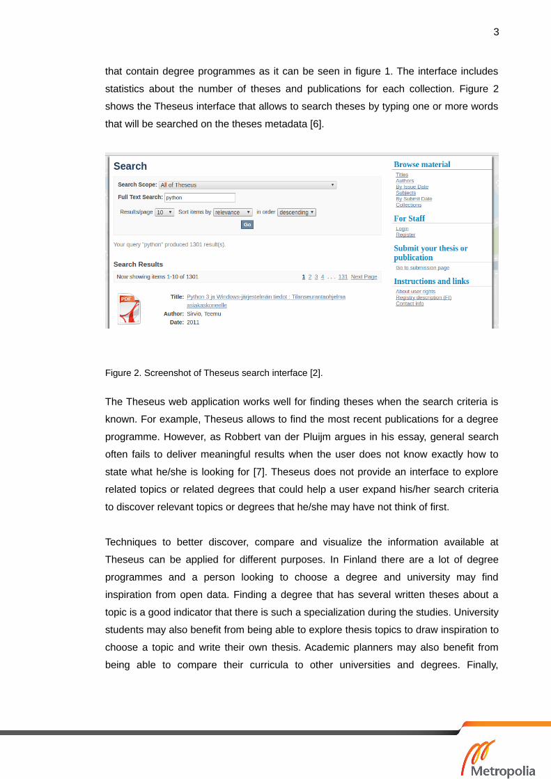
that contain degree programmes as it can be seen in figure 1. The interface includes

statistics about the number of theses and publications for each collection. Figure 2

shows the Theseus interface that allows to search theses by typing one or more words

that will be searched on the theses metadata [6].

Figure 2. Screenshot of Theseus search interface [2].

The Theseus web application works well for finding theses when the search criteria is

known. For example, Theseus allows to find the most recent publications for a degree

programme. However, as Robbert van der Pluijm argues in his essay, general search

often fails to deliver meaningful results when the user does not know exactly how to

state what he/she is looking for [7]. Theseus does not provide an interface to explore

related topics or related degrees that could help a user expand his/her search criteria

to discover relevant topics or degrees that he/she may have not think of first.

Techniques to better discover, compare and visualize the information available at

Theseus can be applied for different purposes. In Finland there are a lot of degree

programmes and a person looking to choose a degree and university may find

inspiration from open data. Finding a degree that has several written theses about a

topic is a good indicator that there is such a specialization during the studies. University

students may also benefit from being able to explore thesis topics to draw inspiration to

choose a topic and write their own thesis. Academic planners may also benefit from

being able to compare their curricula to other universities and degrees. Finally,

4

employers may also benefit from identifying degree programs with specific

specializations to contact and create partnerships.

A comparable global open repository known as arXiv contains over one million papers

mostly in the fields of Physics, Mathematics and Computer Science. The arXiv

repository has been operating since 1991 and it adds on average around 300

publications per day [8]. More recently, the addition of an average of 50 thesis per day

since 2009 in a single country indicates that there is a lot of information in the Theseus

repository.

An example of a discovery tool is the Paperscape project that visualizes, in an

interactive map, the arXiv papers grouped by area of knowledge based on the

references of the papers. In figure 3 each paper is represented by a circle, with its area

proportional to the number of citations. Paper positions are based on references so that

a paper is attracted by all other papers that reference it. The blue area in the centre of

figure 3 contains papers in the high energy theory category. [9]

Figure 3. Screenshot of Parperscape academic papers map [9].

More recently, a French start-up named Impala has developed a platform to help high

school students discover the different professions and degrees in France [10]. For that,

they use a map of professions created from the description of those professions

provided by Onisep, a public editor that gathers information about study programmes

5

and professions in France [11]. In figure 4 professions are represented by circles that

are grouped and coloured based on the domain area. Clicking on a circle allows to

access the degrees that lead to that profession and other relevant information.

Figure 4. Screenshot of Impala professions map [10].

The Theseus repository is unique in itself because of its completeness and the

richness of theses metadata which contains already annotated topics by the authors

and librarians. The Theseus data is also continuously updated with new theses so that

information regarding degree topics stays up to date.

2.2 Data Mining Overview

Data mining is the process of discovering patterns and relationships in large volumes of

data by using methods from the areas of computer science, statistics and artificial

intelligence [12]. Data mining is a general term and it can often be confusing. Moreover,

since the data mining term first appeared in the 1990s, its meaning has evolved

together with the appearance of new data challenges and methods. In the early days,

data mining was often linked to Business Intelligence (BI) applications, where patterns

were discovered by the computation of formulas and aggregations over big commercial

datasets to create operational dashboards and reports consumed by humans. Later on,

the development of more heterogeneous datasets, such as those generated by the

Internet where data is often of less quality than the data governed by a company,

required the application of machine learning techniques to extract knowledge.

6

Machine learning algorithms can be divided into supervised, unsupervised and

reinforcement learning. In supervised learning the algorithm is trained on some input

data to predict an expected output. Once the algorithm is trained, it is expected that it

will be able to predict an output for new data in which the output is not previously

known. An example of supervised learning is the problem of learning to recognize cats

and dogs in pictures by providing a set of already classified pictures. In unsupervised

learning the algorithm allows to discover patterns to better understand and represent

the data. An example of unsupervised learning is the detection of groups of users that

have a similar shopping behaviour in an e-commerce platform. Unsupervised learning

algorithms are harder to evaluate because the correct answer is not known and thus

unsupervised learning is often evaluated based on its utility to better understand the

data, detect patterns and improve the results from other techniques. In reinforcement

learning the algorithm allows an agent to learn some behaviour on the data based on

feedback from the environment. An example of reinforcement learning is a program

learning to play a game by adjusting its actions by playing several games and

observing the final score. [13]

In this thesis, unsupervised learning techniques such as dimensionality reduction and

clustering will be applied. Dimensionality reduction techniques such as PCA and t-SNE

transform the data to a representation with fewer variables in order to select features,

improve the results of other machine learning algorithms or allow visualizing the data in

two or three dimensions. Applied clustering techniques such us k-means, DBSCAN and

hierarchical clustering are used to discover groups of similar elements to better

understand and represent the data.

Together with the evolution of applied methods in data mining, there has been a

development of the data mining process. Based on a poll by KDnuggets in 2014 the

most used data mining process was the Cross Industry Standard Process for Data

Mining (CRISP-DM) [14]. The CRISP-DM process was conceived in 1996 and

structures the data mining process in six phases that are illustrated in figure 5.

7

Figure 5. Relationship between the different phases of CRISP-DM. [15]

Surprisingly, the second most commonly used process found by the poll was labelled

as “My own”, suggesting that several data analysts, engineers and scientists have

developed their own methodologies. For example, Benjamin Bengfort (2015) criticizes

the so called traditional “data science” pipeline as it does not meet the requirements for

building modern data products based on machine learning [16]. He argues that those

new products should be able to incorporate new data generated by having the user

interact with the product. Those new systems able to generate new data are often

referred as data products.

To describe the process of building data products, Bengfort introduces a new

classification of a data pipeline in two phases: the build phase and the operational

phase; and four stages shown in figure 6: interaction, data, storage and computation.

Bengfort considers this pipeline to be more suited for building data products because

human feedback can be introduced back to the system to improve it. This feedback

allows to create systems that automatically improve over time, by exploiting user

generated data. This data is generated by having the user interact with the product, for

example, annotating data, gathering clicks or user actions.

8

Figure 6. Relationship between the different phases of the Bengfort data product pipeline. [16]

As previously stated, the most popular data mining process dates back from 1996. This

has led many professionals and companies to develop their custom or in-house

methodologies. Little has been written regarding formal data mining process compared

to the extensive bibliography that deals with specific algorithms or techniques. For that

reason, this thesis presents the results of all phases of a data mining project and their

relationships instead of focusing on only one.

Over the last few years, a new series of data mining techniques known as Deep

Learning have rapidly developed. Those techniques have improved the performance of

algorithms to annotate text [17], images [18] and sound data [19]. It is expected that in

the following years, those new deep learning techniques will also reflect on new data

mining methodologies that will be used to create AI products.

9

3 Methodology and Tools

In order to create the final application the work was performed and will be presented in

six different phases:

1. Collecting the Data.

2. Exploring the Data.

3. Cleaning the Data.

4. Analysing the Data.

5. Modelling the Data.

6. Visualizing the Data.

In theory, the phases above are performed sequentially in order. For example, it is first

required to have some data to be able to explore it. In practice, the data process is

iterative in nature, that is, after going through one phase it is possible, and advisable, to

go back to improve on the previous phases. For example, after allowing the user to

interact with the data, data inconsistencies may be found that require further cleaning

of the data. Another example is that after analysing the data it may be discovered that

there is not enough collected data and it is required to evaluate other sources to collect

more data to improve the results.

Multiple iterations are needed, and each builds up a more complex and better suited

model at each phase. The work presented here, includes the compiled results from all

iterations. The six different phases can be divided into three subgroups that are very

interdependent with different goals: collecting data to be able to explore it, cleaning

data to be able to analyse it and modelling data to be able to visualize it. First,

exploration generates information that is used to better understand the data. Then,

analysis generates new data, clusters for example, that is used to better represent the

data. Finally, interactive visualizations generate a user experience that allows to get

user feedback over how to improve the product in the next iteration.

Several languages, frameworks and tools exist for working with data. For this thesis,

Python was chosen as the main programming language to collect, explore, clean,

analyse and model the data for its popularity and extent of available libraries and

10

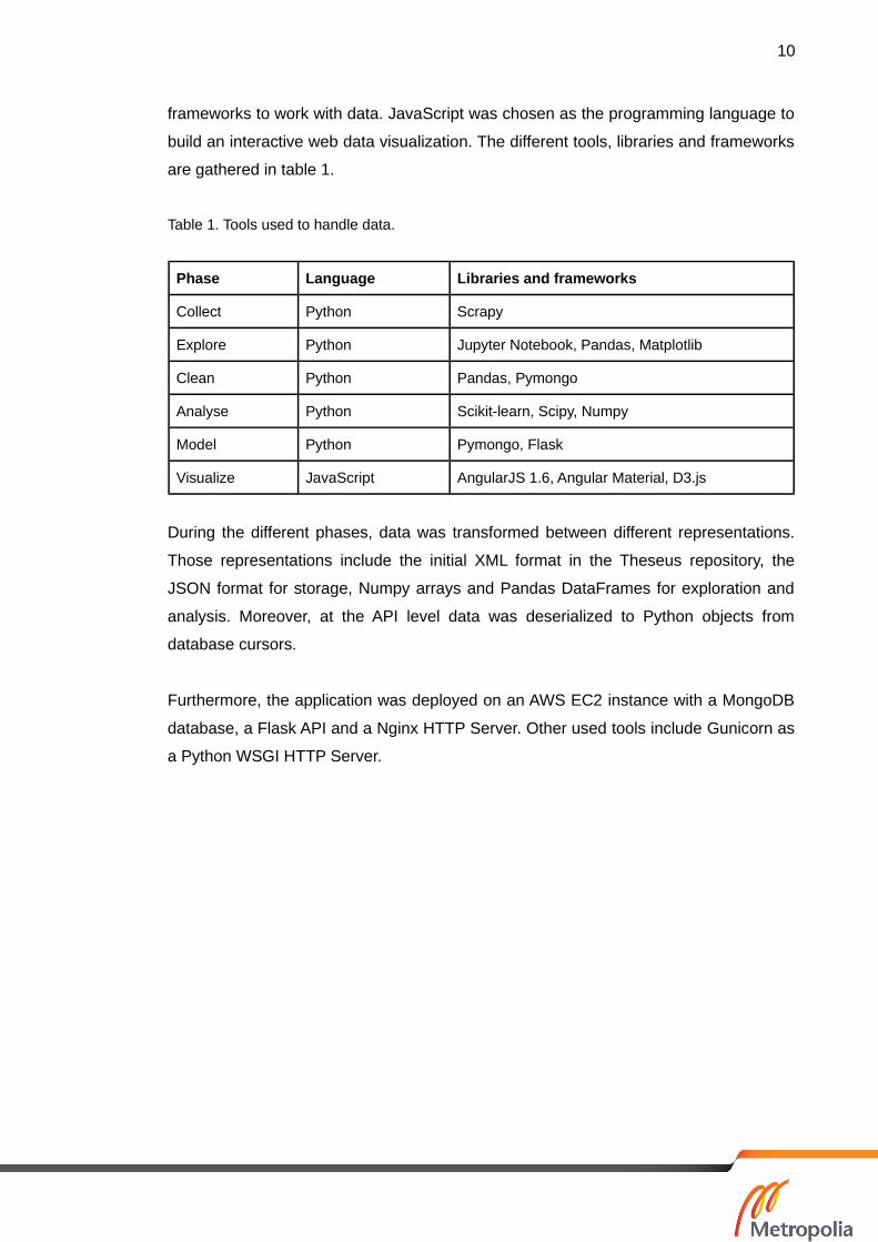
frameworks to work with data. JavaScript was chosen as the programming language to

build an interactive web data visualization. The different tools, libraries and frameworks

are gathered in table 1.

Table 1. Tools used to handle data.

Phase Language Libraries and frameworks

Collect Python Scrapy

Explore Python Jupyter Notebook, Pandas, Matplotlib

Clean Python Pandas, Pymongo

Analyse Python Scikit-learn, Scipy, Numpy

Model Python Pymongo, Flask

Visualize JavaScript AngularJS 1.6, Angular Material, D3.js

During the different phases, data was transformed between different representations.

Those representations include the initial XML format in the Theseus repository, the

JSON format for storage, Numpy arrays and Pandas DataFrames for exploration and

analysis. Moreover, at the API level data was deserialized to Python objects from

database cursors.

Furthermore, the application was deployed on an AWS EC2 instance with a MongoDB

database, a Flask API and a Nginx HTTP Server. Other used tools include Gunicorn as

a Python WSGI HTTP Server.

11

4 Building Ammattiko

The results in this section are based on the data collected by 6 April 2017. All the code

is open source and available on Github [20].

4.1 Collecting the Data

Theseus uses the DSpace [21] open source software to create an open access

repository. Theses metadata can be harvested using the OAI-PMH protocol supported

by DSpace and made available by Theseus in XML format through HTTP [22].

Previous work by Gebresilassie (2014) goes into more detail about Harvesting

Statistical Metadata from Theseus [23].

To collect the data needed for this project, a web scraper was developed to extract the

data from the Theseus repository in XML and store it in JSON. The scraper was built

using the Python framework Scrapy. Two different spiders were developed, one for the

theses metadata and other for the collections metadata with information about

universities and programmes. The extracted data was stored in JSON. The JSON

format was chosen instead of CSV because the extracted data fields contained array

values that are easier to store in JSON. Moreover, the JSON format was chosen over

the native XML because it can be directly loaded into Pandas Dataframes for

exploration and imported into databases such as MongoDB for querying. A Scrapy

pipeline was also developed to clean and load the scraped data both into a file for

exploration and into the database for modelling. The scraper can be launched multiple

times, and each time it will add new theses to the database.

4.2 Exploring the Data

In this phase, different statistics and graphs are computed on the scraped data to get a

better understanding of the data. Data exploration lies within the framework of

Exploratory Data Analysis (EDA) that allows to formulate different hypotheses about

the data. The results in this phase are either produced using the MongoDB aggregation

framework or the Pandas library. The graphs are plotted with Matplotlib.

12

After running the scraper, 118,212 theses metadata have been collected. An example

single thesis record contains the following information:

{

"_id": "oai:www.theseus.fi:10024/474",

"dates": ["2013­08­19T10:18:05Z"],

"collections": ["com_10024_14", "col_10024_174"],

"urls": ["http://www.theseus.fi/handle/10024/474"],

"authors": ["Hakala, Lilli"],

"organizations": ["Satakunnan ammattikorkeakoulu"],

"programmes": ["Viestinnän koulutusohjelma"],

"orientations": [""],

"abstracts_fi": [

"Opinnäytetyössä kartoitettiin verkkovideoiden”],

"abstracts_en": ["The aim of this thesis is to chart … "],

"abstracts_sv": [],

"languages": ["fi"],

"subjects": [

"verkkojulkaiseminen", "verkkoviestintä", "verkkojulkaisut",

"video", "verkkolehdet"],

"keywords" : [],

"titles" : [

"Hyvä ja toimiva video sanomalehden verkkopalvelussa"],

"document_urls" : [

"http://www.theseus.fi/bitstream/10024/474/1/Hakala+Lilli.pdf"],

"years" : ["2008"],

}

Listing 1. Example thesis document metadata.

Each thesis contains a unique identifier such as oai:www.theseus.fi:10024/474 that will

be stored in the database on the field _id. The rest of the field names are pluralized

because although for this example thesis only the fields collections, subjects and

keywords contain more than one element, this is not the case for all theses.

13

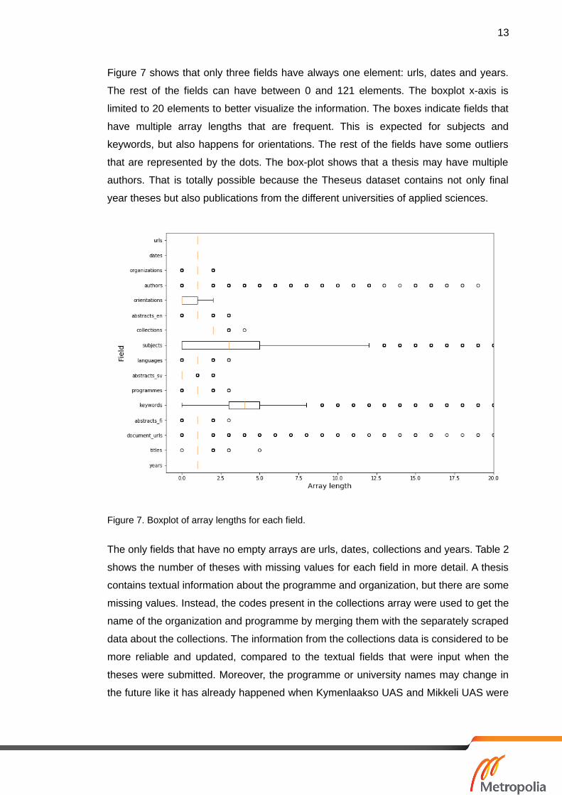
Figure 7 shows that only three fields have always one element: urls, dates and years.

The rest of the fields can have between 0 and 121 elements. The boxplot x-axis is

limited to 20 elements to better visualize the information. The boxes indicate fields that

have multiple array lengths that are frequent. This is expected for subjects and

keywords, but also happens for orientations. The rest of the fields have some outliers

that are represented by the dots. The box-plot shows that a thesis may have multiple

authors. That is totally possible because the Theseus dataset contains not only final

year theses but also publications from the different universities of applied sciences.

Figure 7. Boxplot of array lengths for each field.

The only fields that have no empty arrays are urls, dates, collections and years. Table 2

shows the number of theses with missing values for each field in more detail. A thesis

contains textual information about the programme and organization, but there are some

missing values. Instead, the codes present in the collections array were used to get the

name of the organization and programme by merging them with the separately scraped

data about the collections. The information from the collections data is considered to be

more reliable and updated, compared to the textual fields that were input when the

theses were submitted. Moreover, the programme or university names may change in

the future like it has already happened when Kymenlaakso UAS and Mikkeli UAS were

14

merged to form XAMK (South-Eastern Finland UAS) from the 1 January 2017 [24]. At

the moment, this change has not being reflected on the Theseus dataset yet.

Table 2. Missing values count for each field.

Field Missing values count

abstracts_sv 113359

orientations 62983

subjects 50409

abstracts_fi 15134

keywords 13435

abstracts_en 13262

programmes 2726

authors 339

organizations 140

document_urls 43

languages 20

titles 1

years 0

collections 0

dates 0

urls 0

The statistics for the language field in figure 7 and table 2 indicate that some of the

118,212 collected theses have no language and that some other theses have more

than one language on the metadata. That is probably an inconsistency in the data that

may need further processing so that this data can be exploited. These kind of

inconsistencies can be due to a data entry error when the thesis was submitted or due

to a data migration. Often present in real datasets, these inconsistencies happen when

the data is part of a system that does not validate sufficient constraints on data input.

The years field satisfies the constraint of having only one value for a given thesis. In

order to know whether the field values are clean, it can also be useful to get the

number of distinct values for each field.

15

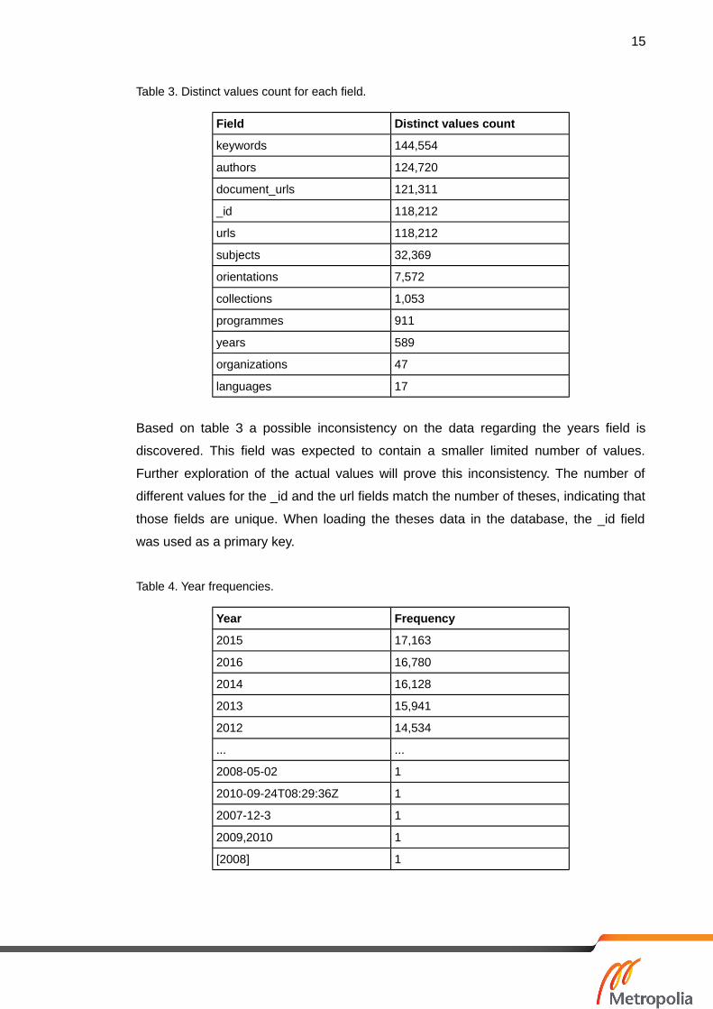
Table 3. Distinct values count for each field.

Field Distinct values count

keywords 144,554

authors 124,720

document_urls 121,311

_id 118,212

urls 118,212

subjects 32,369

orientations 7,572

collections 1,053

programmes 911

years 589

organizations 47

languages 17

Based on table 3 a possible inconsistency on the data regarding the years field is

discovered. This field was expected to contain a smaller limited number of values.

Further exploration of the actual values will prove this inconsistency. The number of

different values for the _id and the url fields match the number of theses, indicating that

those fields are unique. When loading the theses data in the database, the _id field

was used as a primary key.

Table 4. Year frequencies.

Year Frequency

2015 17,163

2016 16,780

2014 16,128

2013 15,941

2012 14,534

... ...

2008-05-02 1

2010-09-24T08:29:36Z 1

2007-12-3 1

2009,2010 1

[2008] 1

16

Table 4 shows the more popular year values are clean, and the inconsistency comes

from some outliers. To understand the data it is important to sample values with

different frequencies. The outliers still seem to contain information about the year but

in a different format that needs to be parsed. Because the Theseus platform to submit

theses was first launched in 2009 and most of the outliers suggest previous years, this

format inconsistency may have come from a migration script that was used to load

theses from existing university repositories.

Table 5. Language frequencies.

Language Frequency

fi 101,623

en 12,177

sv 4,348

689

fr 13

fi, en 11

ru 10

de 6

other 4

es 1

se 1

swe 1

selkokieli 1

et 1

zh 1

eng 1

akuuttihoito 1

Table 3 showed that the language field had the less number of different values. Table 5

shows that there are three frequent languages for theses: Finnish (fi), English (en) and

Swedish (sv). There are also 689 theses that have one of the languages as an empty

string “”.

Regarding the exploration of thesis subjects and keywords it may be interesting to have

a closer look at the histogram of number of keywords and subjects. Comparison of

figures 8 and 9, shows that it is much more frequent for a thesis to contain no subjects

17

than no keywords. Apart from zero, the most frequent number of keywords and

subjects for a thesis is four.

Figure 8. Subjects histogram.

Figure 9. Keywords histogram.

It is expected that some keywords and subjects are more frequent than others. This

hypothesis can be confirmed by plotting the histogram of keywords and subjects

frequencies.

18

Figure 10. Subject frequency histogram.

Figure 11. Keyword frequency histogram.

Figures 10 and 11 show that there are multiple subjects and keywords with low

frequencies. Both figures have a logarithmic scale on the y-axis. It is Important to note

that over 51% of subjects (16,597 subjects out of 32,369) and over 72% of keywords

(104,872 keywords out of 144,554) appear only in one thesis.

Keywords and subjects frequencies are included in tables 6 and 7. Keywords and

subjects are not normalized and can contain spaces, empty values and capitalized

letters.

19

Table 6. Subject frequencies.

Subject Frequency

markkinointi 2,570

kehittäminen 2,510

nuoret 1,909

lapset 1,865

laatu 1,715

... ...

Ultrasonic transducers 1

Dental Caries 1

Medios-hanke 1

pain 1

agrologer 1

Table 7. Keyword frequencies.

Keyword Frequency

markkinointi 1449

asiakastyytyväisyys 1339

kehittäminen 1323

varhaiskasvatus 1285

työhyvinvointi 1231

... ...

environmental friendliness 1

banking risks 1

Cross-border cooperation 1

eläkelaitos 1

flirttikouluttaja 1

4.3 Cleaning the Data

Data cleaning is the process of correcting inaccurate records from a dataset and

dealing with inconsistencies in order to fit the data into a model. A survey published by

CrowdFlower in 2016 reported that 60% of a data scientist’s time deals with cleaning

and organizing data [25, 6]. Data cleaning simplifies and improves the data analysis

phase as often simpler algorithms perform better on cleaned data than complex

20

algorithms on messy data [26]. On the one hand, a bigger dataset can sometimes

compensate for the lack of data quality as Halevy argues in his essay The

Unreasonable Effectiveness of Data [27]. On the other hand, a combination of better

data and algorithms is sometimes needed to get better results [28].

The results from the data exploration phase have shown some data inconsistencies

that need to be treated, including: wrong values, missing values, duplicate values and

wrongly formatted values. While modern databases such as NoSQL allow to store data

without a model, it is still important to clean the data. When writing application code

that will query and handle data, it is important to know certain rules regarding the data

because otherwise programming errors will be raised. Furthermore, some data

inconsistencies may result in a poor user experience while building a product that

exposes them.

In order to build a product to explore thesis topics, only certain fields need to be

cleaned. In particular, this phase presents the processing done for the following fields:

keywords, subjects, languages, years, dates, titles, universities and degrees.

Figure 12. Topics histogram.

Cleaning Keywords and Subjects

Keywords and subjects were normalized by transforming the text to lower-case, joining

both arrays and removing empty values and duplicates to create a new topics field.

21

After the process, figure 12 shows that there are fewer theses with no topic compared

to the results in figures 8 and 9.

Cleaning Languages

It is expected for consistency that a thesis is written in a single language. Given that

the thesis metadata may indicate multiple languages, only one of them was kept in a

new language field. For simplicity, the language kept was the first one in the array.

Other techniques such as giving a priority to a language or inferring the thesis

language from other fields could have been employed but were not a priority for the

application built. When building the web application to explore Theseus data only three

languages will be selectable: Finnish, English and Swedish.

Cleaning Years

It is expected that the value of the year field contains only integers over a reasonable

range of values. For that, the year information was parsed with a regular expression.

This field would be important for mining topics trends over time.

Cleaning Dates

It is expected that this field contains a date object including date and time that can be

used to sort the theses in chronological order. For that, the field was parsed into a

Python datetime object that will be loaded as a MongoDB Date object.

Cleaning Titles

It is expected that a thesis has one title. While a thesis can have a title in different

languages, for simplicity only one title was kept. The first title in the titles array was

selected after empty values were removed.

Cleaning Universities

The university code was extracted from the thesis collections array to be the one that

started with com (abbreviation of community) such as com_10024_14. The DSpace

repository is structured in a hierarchy of communities that contain collections [29]. The

22

university name was inferred by joining the thesis data with the separately scraped

collection data.

Cleaning Degrees

The degree code was extracted from the theses collections array to be the one that

started with col (abbreviation of collection) such as col_10024_174. For simplicity, only

the first occurrence was kept. The degree name was inferred by joining the thesis data

with the separately scraped collection data.

4.4 Analyzing the Data

This phase explores the relationships between degrees based on topics to be able to

identify related degrees. Intuitively, related degrees are those that have a lot thesis with

topics in common. Data will be first preprocessed to then perform dimensionality

reduction to project degrees in a 2-dimensional map and clustering to form groups of

related degrees based on computed distances between degrees. Degree projections

will be evaluated based on whether different groups can be identified visually. Those

groups are supposed to be separated from other groups. Clustering techniques will be

then used to programmatically assign the degrees to groups, named clusters.

4.4.1 Preprocessing the Data for Analysis

First, the thesis data was loaded into a Pandas DataFrame. A DataFrame is a data

structure similar to a table that contains labelled columns and rows. Then, the thesis

DataFrame was grouped by degree to get a list of all repeated topics that occur for a

given degree in a Pandas DataFrame (topics column) and the number of different

thesis (n_thesis column). Table 8 shows five example rows of the degrees DataFrame

with various number of thesis.

23

Table 8. DataFrame of degree topics.

degree_id topics n_thesis

col_10024_100 [lääkehoito, development project, implementati... 46

col_10024_100099 [produktion, tga, biodegradable plastics, star... 1

col_10024_100100 [non-technical skills, caracters and character... 4

col_10024_101 [ammattitaito, konepajat, työssäoppiminen, aik... 228

col_10024_102 [arviointitutkimus, tietokoneen käyttö, käytet... 35

In order to run machine learning algorithms using libraries such as Scikit-learn, the data

needs to be represented in a matrix that contains only numbers. Data was

preprocessed using the CountVectorizer class to get a matrix with degrees in the rows

and topics with a global frequency higher than two in the columns [30]. The values in

the generated matrix indicate how many times a topic is present in a degree. The

generated matrix was stored in compressed sparse row format that allows to save

space by only storing the entries that are non zero. In this case, storing only the

337,720 non zero elements instead of the total 42,936,048 (1,026 degrees * 41,848

topics) allows to save 99,3% of memory space. Moreover, computations run much

faster.

A common numerical statistic known as TF-IDF was then used to transform the topics

count matrix to a normalized TF-IDF representation. The term TF-IDF stands for term

frequency-inverse document frequency. For example, this technique is used by search

engines to weigh the importance of results given a user query [31]. Topics that have a

low frequency for all degrees but occur often for some degrees will be given a high TF-

IDF. The applied Scikit-learn TfidfTransformer uses the formula tf-idf(d, t) = tf(t) * idf(d,

t) to compute the TF-IDF score of a topic t where tf(t) is the topic frequency for a

degree and idf(d, t) is computed as idf(d, t) = log [ n / df(d, t) ] + 1 where n is the total

number of theses and df(d, t) is the number of theses that contain a topic d [32]. After

the TF-IDF transformation, the values in the degree topics matrix are bounded between

0 and 1.

4.4.2 Dimensionality Reduction with PCA

To explore the relation between degrees, each degree vector produced by TF-IDF was

transformed into a vector of two dimensions that can be visualized on the plane.

24

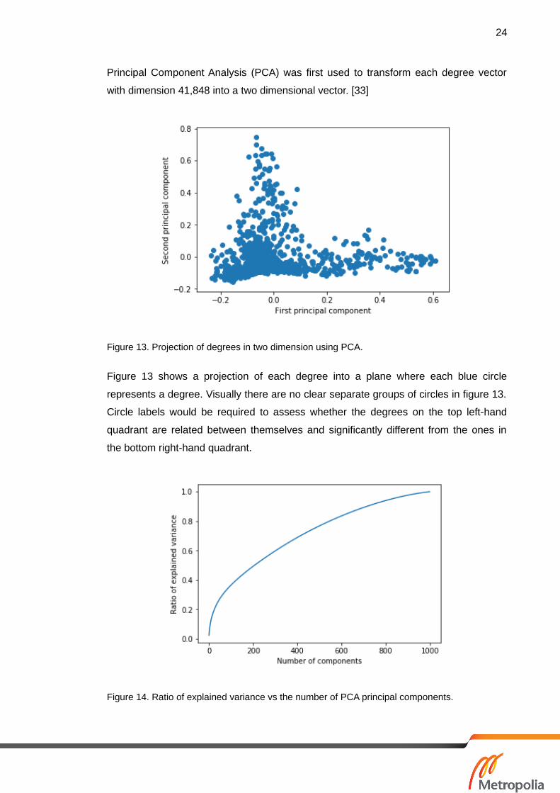
Principal Component Analysis (PCA) was first used to transform each degree vector

with dimension 41,848 into a two dimensional vector. [33]

Figure 13. Projection of degrees in two dimension using PCA.

Figure 13 shows a projection of each degree into a plane where each blue circle

represents a degree. Visually there are no clear separate groups of circles in figure 13.

Circle labels would be required to assess whether the degrees on the top left-hand

quadrant are related between themselves and significantly different from the ones in

the bottom right-hand quadrant.

Figure 14. Ratio of explained variance vs the number of PCA principal components.

25

When performing PCA it is important to know the percentage of variance explained by

each component. In this case, the two principal components explain less than 5% of

the variance, meaning that a lot of information regarding the structure of degrees is lost

by considering only two components. Figure 14 includes a plot of the cumulative ratio

of variance explained by the first 1,000 principal components. To keep at least 99% of

the variance the first 953 principal components need to be kept. At first sight, PCA does

not seem to be a sufficient technique to represent degrees on two dimensions that

allow to visualize separate groups but may serve as a preprocessing step to more

advanced techniques. Indeed, it is recommended to use PCA before applying other

techniques such as t-SNE to suppress some noise and speed up the computation of

pairwise distances between degrees [34, 2589].

4.4.3 Dimensionality Reduction with t-SNE

T-distributed stochastic neighbour embedding (t-SNE) is a dimensionality reduction

technique specially useful for embedding high-dimensional data into a space of two or

three dimensions to visualize in a scatter plot. The algorithm behind t-SNE builds up a

low dimensional distribution over the pair of points to minimize the Kullback-Lieber

divergence with the original distribution [34, 2581]. In this way, points are mapped to

locations that try to respect the original distances in the high-dimensional space. The

optimization problem is solved using the gradient descent method and different

initializations might result in different local minima of the cost function. In the case of t-

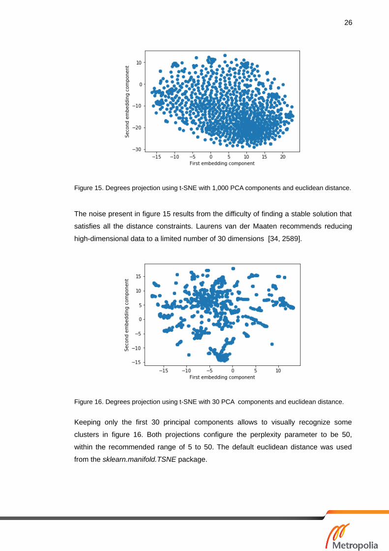
SNE, keeping all the variance is not necessarily recommended. For example, keeping

1,000 components in PCA results in a projection which includes some areas with a high

density of points but also a lot points uniformly distributed between those areas as it

can be seen in figure 15.

26

Figure 15. Degrees projection using t-SNE with 1,000 PCA components and euclidean distance.

The noise present in figure 15 results from the difficulty of finding a stable solution that

satisfies all the distance constraints. Laurens van der Maaten recommends reducing

high-dimensional data to a limited number of 30 dimensions [34, 2589].

Figure 16. Degrees projection using t-SNE with 30 PCA components and euclidean distance.

Keeping only the first 30 principal components allows to visually recognize some

clusters in figure 16. Both projections configure the perplexity parameter to be 50,

within the recommended range of 5 to 50. The default euclidean distance was used

from the sklearn.manifold.TSNE package.

27

The quality of the t-SNE projection to represent degrees that are related will be

evaluated manually in the visualizing the data phase with the interactive web

application that allows to see the name of the degrees by hovering over them.

Exploration of the circles discovered that degrees with a lot of theses and topics are

situated on the borders of the plot to satisfy the distance constraints between them

while degrees with less information are situated in a high-density area around the

centre.

The cosine distance was also tested to perform t-SNE. The results and shape of the

clusters differ from those achieved by using the euclidean distance as it can be seen in

figure 17.

Figure 17. Degrees projection with 30 PCA components, cosine distance and perplexity 200.

Exploration of the projected degrees proved that higher values of perplexity produced

projections that were more radial in shape like in figure 16 with the degrees with less

topics and theses in the centre of the projection and more separation between clusters.

A good balance between having separated clusters and keeping the proximity between

different clusters was found for a perplexity value of 20 applied to 50 principal

components. This projection is shown in figure 18 and will be used for the web

application.

28

Figure 18. Degrees projection using t-SNE with 50 components and perplexity of 20.

4.4.4 Clustering Degrees with k-means

K-means is a popular clustering algorithm that requires to set the number of desired

clusters in advance. The clusters are built iteratively by first initializing randomly the

cluster centroids (“central” point), then assigning points to the closest centroid and

finally updating the centroids as the average of all the cluster points. The k-means

algorithm is designed to only work with euclidean distances because euclidean

distances can be averaged to update the centroids after each iteration. It is known that

the euclidean distance does not perform best on high-dimensional data because

distances between any two points tend to converge. [35]

Regardless of those limitations, some interesting information can be extracted from k-

means. Particularly, k-means can perform well to detect outliers [36].

In figure 19 k-means was used to label degrees in ten different colour coded clusters

plotted on the t-SNE projection using the cosine distance. Manual exploration

discovered that the green cluster at the left in figure 19 corresponded to business

studies, the dark blue cluster at the top corresponded to social studies, the green one

at the bottom to studies in information technology, the red one at the bottom to studies

in construction, architecture, machine operator and electricity. The spread yellow

cluster corresponded mostly to degrees in English. Finally, the lighter blue cluster that

29

contains most of the points corresponded mainly to outliers, degrees that did not have

enough theses or topics and were harder to classify.

Figure 19. Degrees k-means clustering colors and t-SNE projection using the cosine metric.

Figure 20. Degrees k-means clustering colors and t-SNE projection using the euclidean metric.

In figure 20 k-means was used to show how cluster labels in the original high

dimensional space are respected by t-SNE. Clustering results did not perfectly match

the results from t-SNE projections but still there are some clear clusters that are

concentrated in one location such the green and cyan coloured ones. Other clusters

such as the red and yellow one are splitted in different separated groups on the

30

projection. This can be interpreted as t-SNE being able to capture some of the higher

level clustering but probably focusing on a finer level clustering than ten different

groups.

4.4.5 Clustering Degrees with DBSCAN

Density-based spatial clustering of applications with noise (DBSCAN) belongs to a

different family of clustering algorithms than k-means. The algorithm groups points that

are close together and can find clusters of different shapes. Clusters are composed of

areas with high density of points separated by areas with low density. Furthermore, the

number of desired clusters does not need to be specified in advance. Instead, two

parameters are required: the minimum number of elements to form a cluster and the

maximum distance between two elements in the cluster. [37]

In the case of clustering degrees, the minimum number of degrees to form a cluster

can be set to two and the maximum distance was set empirically to 0.04. Figure 21

shows the result of running DBSCAN on top of the output of t-SNE for degrees that

have at least 50 theses. By removing degrees that have not enough theses and lay

between clusters, DBSCAN allows to assign degrees to the clusters that are

recognized visually.

Figure 21. DBCAN clusters on top of t-SNE data for degrees with more than 50 theses.

31

4.4.6 Hierarchical Clustering of Degrees

Hierarchical clustering is a technique that seeks to build a hierarchy of clusters. The

algorithm iteratively merges clusters based on a metric and a linkage criteria. The

advantages of hierarchical clustering include that it is not necessary to specify

parameters such as the number of clusters or maximum distance between elements in

a cluster in advance. Instead the result of the clustering can be later used to divide the

degrees in multiple different clusters based on different splitting criteria. [38]

The degrees were clustered using the cosine distance and the ward linkage criteria.

The clustering was done using the Python library Scipy. Hierarchical clustering can be

visualized using a dendrogram as seen in figure 22. The dendrogram represents a tree

of degrees that are joined together depending on the chosen distance. Nodes of the

tree that are closer are more related.

Figure 22. Extract from the dendrogram of degrees.

Figure 22 allows to see the structure of a subset of degrees. Following the branches of

the dendrogram the degrees can be first separated in two clusters: the purple one with

32

degrees in the business area and the yellow one with degrees in IT. Furthermore,

degrees in IT can then be further separated on two more precise clusters: the IT

degrees in Finnish and IT the degrees in English. Furthermore, the IT degrees in

English can be separated on Information Technology and Business Information

Technology. Hierarchical clusters then seems to successfully capture the different

levels of degrees based on topics.

Based on the results, hierarchical clustering could be further used to create a user

experience where a user first selects for example between 10 degree clusters. After it

has selected one of the clusters, then another 10 sub-clusters are shown and so on

until the desired degree is found. This technique was explored but is not included

because of the difficulty to generate labels for each cluster at each level. One possible

technique to generate labels consists of showing the n most popular topics for each

cluster.

4.5 Modelling the Data

In order to build a data product that will query data it is important to model the data in a

database. For this project MongoDB was chosen because of its flexibility to store data

and its powerful aggregation framework. MongoDB is a NoSQL database that stores

data in databases that use collections of documents in JSON format. On the one hand,

the flexibility of MongoDB compared to relational databases allows to evolve the data

schema fast when it is not known in advance. On the other hand, MongoDB lacks

features such as transactions and data migrations that need to be handled

programmatically.

One database named theseus and four collections were created to store the different

entities: theses, universities, degrees and topics. The theses collection contains a

series of thesis documents as seen in listing 2 and allows to get more information by

joining the data with the degrees and universities collections using the $lookup

aggregation.

33

{

"_id" : "oai:www.theseus.fi:10024/474",

"collections" : ["com_10024_14", "col_10024_174"],

"url" : "http://www.theseus.fi/handle/10024/474",

"authors" : ["Hakala, Lilli"],

"title" : "Hyvä ja toimiva video sanomalehden verkkopalvelussa",

"topics"   :   ["verkkolehdet",   "video",   "verkkojulkaisut",

"verkkoviestintä",  "verkkojulkaiseminen"],

"university" : {“_id" : "com_10024_14"},

"degree" : {"_id" : "col_10024_174"},

"year" : 2008,

"date" : ISODate("2013­08­19T10:18:05Z"),

"language" : "fi"

}

Listing 2. Most important fields for a thesis document.

Most of the information was processed during the data cleaning phase. Several

indexes were created to speed up the queries on the following fields: topics,

university._id, degree._id, language and date.

The university's collection only contains the university id and name as can be seen in

listing 3.

{

"_id" : "com_10024_1",

  "name" : "Seinäjoen ammattikorkeakoulu"

  }

Listing 3. Example university document.

The degrees collection contains a series of degree documents with coordinates and

cluster fields generated during the data analysis phase as it can be seen in listing 4.

The degrees data is denormalized and contains the university data which improves the

query performance by avoiding the need to perform a join at query time.

34

{

"_id" : "col_10024_102",

"name" : "Kuntoutus (ylempi AMK)",

"x" : 0.3869592718,

"y" : 0.1993278414,

"cluster" : 2,

"university" : {

"_id" : "com_10024_15",

"name" : "Turun ammattikorkeakoulu"

}

}

Listing 4. Example degree document.

The topics collection in listing 5 was used to be able to get a list of suggested topics in

the front-end topics search bar. The topics count was precomputed and included to be

able to sort the search results by popularity. Regular expression queries were

performed on this collection to find topics.

{ 

"_id" : "markkinointi",

"count" : 3513

}

Listing 5. Example topic document.

To be able to send the database data to the front-end application a web API was

developed with the Python library Flask. Seven endpoints were developed and

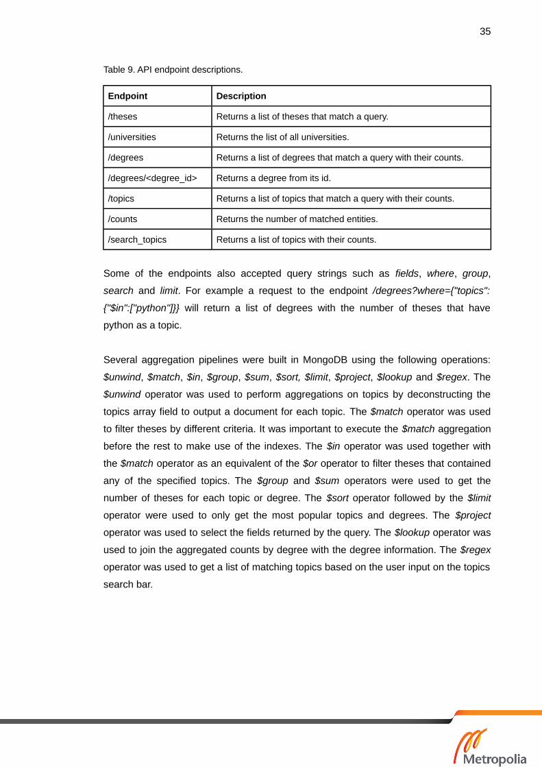
documented in table 9.

35

Table 9. API endpoint descriptions.

Endpoint Description

/theses Returns a list of theses that match a query.

/universities Returns the list of all universities.

/degrees Returns a list of degrees that match a query with their counts.

/degrees/<degree_id> Returns a degree from its id.

/topics Returns a list of topics that match a query with their counts.

/counts Returns the number of matched entities.

/search_topics Returns a list of topics with their counts.

Some of the endpoints also accepted query strings such as fields, where, group,

search and limit. For example a request to the endpoint /degrees?where={"topics":

{"$in":["python"]}} will return a list of degrees with the number of theses that have

python as a topic.

Several aggregation pipelines were built in MongoDB using the following operations:

$unwind, $match, $in, $group, $sum, $sort, $limit, $project, $lookup and $regex. The

$unwind operator was used to perform aggregations on topics by deconstructing the

topics array field to output a document for each topic. The $match operator was used

to filter theses by different criteria. It was important to execute the $match aggregation

before the rest to make use of the indexes. The $in operator was used together with

the $match operator as an equivalent of the $or operator to filter theses that contained

any of the specified topics. The $group and $sum operators were used to get the

number of theses for each topic or degree. The $sort operator followed by the $limit

operator were used to only get the most popular topics and degrees. The $project

operator was used to select the fields returned by the query. The $lookup operator was

used to join the aggregated counts by degree with the degree information. The $regex

operator was used to get a list of matching topics based on the user input on the topics

search bar.

36

4.6 Visualizing the Data

This phase focuses on describing the functionality of the web application built that

contains a dashboard to interactively explore topics and degrees. In the previous

phases the generated graphs were static and did not allow the user to interact with

them. This limited the exploration of the different clusters and the evaluation of the

applied techniques.

To overcome these limitations a web application was built using JavaScript. AngularJS

was used as a framework to control the application logic and D3.js was used to

generate the visual elements. AngularJS version 1.6 proved to be a powerful

combination together with Angular Material to create a dashboard with minimal code.

D3.js was a natural choice to visualize JSON data and integrate graphs in the

dashboard. A state variable was created on the AngularJS scope and synchronized

with the url so that different views of the application could be shared between users

through the url. Graphs were updated by settings watches on the scope values. D3.js

code was integrated in AngularJS by creating two custom directives for the bubble

chart and the bar graph.

The dashboard shown in figure 23 is divided into two parts: filters and reports. Filters

allow the user to search for theses by topics, filter theses by university and filter theses

by language. The dashboard contains three reports: degrees, topics and theses.

Figure 23. Ammattiko dashboard page.

37

Degrees Report

The degrees report visualizes degrees as circles on a map with coordinates computed

by t-SNE on the Analysing the Data phase. The area of the circle was set to be

proportional to the number of theses published for the degree. Hovering on a circle

shows a legend with information regarding the name of the degree and the name of the

university. One or more degrees can be selected by clicking on the circles. Selecting

one degree filters the topics and theses reports. Selecting multiple degrees extends the

topics and theses reports with the new degree using the OR logical operator.

Topics Report

The topics report visualizes the most popular topics as horizontal bars. The bars width

(and area) were set to be proportional to the number of theses with a topic. One or

more topics can be selected by clicking on the bars. Selecting one topic filters degrees,

topics and theses reports. Selecting multiple topics extends the degrees, topics and

theses reports with the the new topic using the OR logical operator. By also filtering

topics based on the selected topics, topics co-occurrences were explored to discover

related topics.

Theses Report

The thesis report contained a list of the most recent theses that match the search

criteria sorted by published date. The number of matched theses was included at the

top of the report. Clicking on a thesis opens a new tab with the Theseus page

containing all information for the thesis, including the ability to download the thesis

paper.

Example Use Case

An initial action by a user may be to search for a domain-specific topic to find the

degrees that cover that topic. For example a user interested in IT can search for the

most popular degrees that have published theses in javascript by typing in the search

bar and discover that there are two main clusters of degrees covering this topic. The

search bar returns a list of the matching topics based on the text entered ordered by

popularity. The degrees map in figure 24 shows two initial clusters that correspond

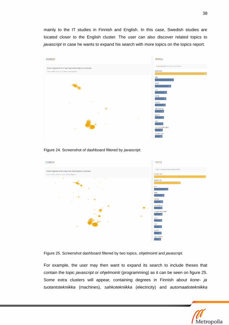
38

mainly to the IT studies in Finnish and English. In this case, Swedish studies are

located closer to the English cluster. The user can also discover related topics to

javascript in case he wants to expand his search with more topics on the topics report.

Figure 24. Screenshot of dashboard filtered by javascript.

Figure 25. Screenshot dashboard filtered by two topics, ohjelmointi and javascript.

For example, the user may then want to expand its search to include theses that

contain the topic javascript or ohjelmointi (programming) as it can be seen on figure 25.

Some extra clusters will appear, containing degrees in Finnish about kone- ja

tuotantotekniikka (machines), sahkotekniikka (electricity) and automaatiotekniikka

39

(automation). Those degrees appear to also teach programming but are not focused on

web development in javascript.

The user can then zoom in a cluster to discover which are the most popular degrees.

After zooming in the bigger cluster the circles gets separated. Zooming in the Finnish

IT cluster shows that it can be further divided into two smaller clusters that correspond

to mainly studies of Tietotekniikka (information technology) at the bottom right and

Tietojenkäsittely (information processing) at the top left in figure 26.

Figure 26. Degrees report filtered by ohjelmointi and javascript, zoom on the Finnish IT cluster.

The dashboard allows to filter also by university and language. For example, the most

popular topics can be found for Metropolia Ammattikorkeakoulu in English as shown in

figure 27 on the mobile version where reports are separated in different tabs. Theses

can be consulted on the theses report as shown in figure 28.

40

Figure 27. Most popular thesis topics for Metropolia Ammattikorkeakoulu.

Figure 28. Example theses report.

41

5 Discussion

The results from this thesis allowed to develop an interactive dashboard to explore

thesis topics and degrees. Multiple challenges were encountered at each stage of the

data mining process. The three phases that took the most time were: exploring the

data, analysing the data and visualizing the data.

The data collection part was found to be a relatively straightforward part. A

considerable amount of time was spent on understanding and evaluating the quality of

the theses data. In the data exploration phase, several data inconsistencies were

raised including missing, duplicate, inaccurate and unformatted values. Those

inconsistencies were expected as the Theseus dataset is a real dataset in continuous

evolution and which allows user input. These inconsistencies also contribute to the

relevance of the work as the presented techniques can be applied to a larger set of

data available. Indeed, it is said that most of the generated data nowadays is

unstructured. Regardless of the data inconsistencies found, the Theseus dataset

contained a lot of information that could be mined. While all the data processing was

performed in memory and thus the Theseus dataset can not be exactly considered

within the framework of big data of 5 Vs [39], it still has some of the characteristics of

big data regarding its volume, variety, velocity, variability and veracity. Furthermore, the

Theseus dataset is unique because it gathers all universities of applied sciences in a

single country, allowing to make relevant comparisons.

The understanding and processing of the data allowed to analyse the data to enrich it

with new inferred properties such as the projection coordinates and the degree cluster

labels. The analysis phase focused on exploring the relationship between degrees

based on topics. Similar techniques could have been used to explore the similarity

between topics to create a topics map or the similarity between theses to create a

thesis map. The biggest challenge found when trying to cluster the degrees was having

to deal with outliers or insufficiently annotated data. Indeed, the Theseus dataset

contains not only degree programmes but also collections of publications. Some

degrees and some collections do not contain sufficient theses or annotated topics for

the algorithms to know how to classify them. These insufficiencies could have been

further treated by extracting the topics from the thesis titles or abstracts. The

42

dimensionality reduction technique t-SNE seemed to perform the best while

representing the degrees on a 2-dimensional map. Most of the time was spent on

selecting the different parameters for the algorithm. After having applied multiple

clustering techniques, it was found that the models are relatively easy to apply but little

has been written about how to choose the right parameters. The choice often depends

on the domain and the understanding of the data and are based on experiments and

heuristics. The three presented clustering techniques showed some benefits and

drawbacks. The most interesting results came from the hierarchical clustering that

allows to perform multiple partitions of the data at different levels. An improvement over

the developed system would exploit the levels of clusters to help the user find a

relevant degree by navigating a hierarchy. Evaluation and generation of meaningful

cluster labels proved to be the most challenging part. In some applications, those

phases are still performed manually by exploring the results. Other clustering

techniques such as affinity propagation, HDBSCAN or biclustering could have been

applied and compared.

The data model chosen to store the data proved MongoDB to be a flexible and

performant database to create a fluid user experience. All data aggregations were able

to be executed under one second due to the creation of database indexes and pre-

aggregation of some data. The developed dashboard allows the user to discover

popular topics and degrees. Multiple options were allowed to filter the data by providing

topics auto-completion and the visualization of related topics and degrees. Special

effort was put into having a balance between the facility to use the dashboard and the

number of options possible. On the one hand, having too many options to interact with

the data can make the user lost. On the other hand, limiting too much the user options

may make the user frustrated. It is expected than sharing the work with more people at

different universities will provide valuable feedback over how to improve the user

experience. For instance, some users found the degree map to contain too many

overlapping circles. The zoom functionality allows to separate the circles. Another

possible improvement would have been to use the hierarchical clustering to only show

labelled clusters of degrees that would display only the cluster members when

selected. The laptop and tablet experience provide a better user experience than the

mobile one because the ability to see all the reports at the same time and the relations

between applying filters on the topics and degrees. Difficulties were found on adapting

the dashboard to mobile screens as the ability to hover over visual elements is not

clear.

43

6 Conclusion

The goal of this thesis was to data mine the Theseus open data repository to discover

popular topics and popular degree programmes. A good understanding of the quality of

the data was achieved by applying different data mining techniques and multiple

reports and graphs were created. The web application built allows the user to

interactively filter published theses by topics, universities, degrees and languages to

subsequently find the most popular degrees and most popular topics. Furthermore, the

degrees map using t-SNE embeddings proved to be useful to convey the information

regarding the study area. Several clustering techniques were applied to cluster degrees

but were not included on the web application because of the difficulty to evaluate the

results and label the clusters. Nevertheless, hierarchical clustering appeared to be the

most promising technique that could be used to deliver a better user experience by

allowing the user to select between the different levels of clusterings, each cluster

labelled with the most popular topics.

A future line of development could explore the evolution of thesis topics over time to

identify trending topics. The evolution of the topics popularity over time for a degree

may be a good indicator of the reactivity of the study plans to adapt to the changes in

the industry and job market.

44

References

1. Arene Ry. Rectors' Conference of Finnish Universities of Applied Sciences [online]. URL: http://www.arene.fi/en

2. Theseus. Open Repository of the Universities of Applied Sciences [online].URL: http://theseus.fi

3. Avoindata. Open Data and interoperability tools [online].URL: https://www.avoindata.fi/en

4. Open Repository Theseus. Success Story of 24 Finnish Universities of Applied Sciences. AMKIT; 2014 [online].URL: http://www.amkit.fi/wp-content/uploads/2016/02/theseus_posteri2_28052014.pdf

5. AMKIT [online].URL: http://www.amkit.fi/en

6. Doria. How to Browse and Search in Theseus [online].URL: http://s1.doria.fi/ohje/Theseus_hakuohje_en.htm

7. Robbert van der Pluijm et al. Search vs Discovery. Bibblio; 2015 [online].URL: https://medium.com/the-graph/search-vs-discovery-1b80e045aea

8. arXiv. The world‘s biggest repository for physics, mathematics and computer science. University Library Erlangen-Nürnberg; 2015 [online].URL: https://ub.fau.de/wp-content/uploads/2015/10/Arxiv-engl.pdf

9. Damien George, Rob Knegjens. About Paperscape [online]. URL: http://blog.paperscape.org/?page_id=2

10. Impala [online].URL: http://impala.in

11. Onisep [online].URL: http://www.onisep.fr/

12. Clifton, Christopher (2010). Encyclopædia Britannica: Definition of Data Mining [online].URL: https://global.britannica.com/technology/data-mining

13. Stuart Russell, Peter Norvig. Artificial Intelligence: A Modern Approach (3rd ed.).Prentice Hall; 2009.

45

14. KDnuggets. What main methodology are you using for your analytics, data mining, or data science projects? Poll; 2014 [online].URL: http://www.kdnuggets.com/polls/2014/analytics-data-mining-data-science-methodology.html

15. CRISP-DM. Cross industry standard for data mining [online].URL: http://crisp-dm.eu

16. Benjamin Bengfort. The Age of the Data Product. District Data Lab; 2015 [online].URL: https://districtdatalabs.silvrback.com/the-age-of-the-data-product

17. Xavier Glorot et al. Domain Adaptation for Large-Scale Sentiment Classification:A Deep Learning Approach. ICML; 2011.

18. Alex Krizhevsky et al. ImageNet Classification with Deep Convolutional Neural Networks. Advances in Neural Information Processing Systems 25. Curran Associates, Inc.; 2012; p. 1097-1105.

19. Honglak Lee. Unsupervised feature learning for audio classification using convolutional deep belief networks. Curran Associates, Inc.; 2009; p. 1096-1104.

20. Bajo Rouvinen Ari. Building a data product to explore thesis topics in Finland. Github [online].URL: https://github.com/arimbr/theseus

21. DSpace documentation [online]. URL: https://wiki.duraspace.org/display/DSPACE

22. Theseus DSpace OAI-PMH Data Provider [online].URL: http://publications.theseus.fi/oai/request

23. Sem Gebresilassie. Harvesting Statistical Metadata from an Online Repository for Data Analysis and Visualization : Concept Application on Theseus. Metropolia Ammattikorkeakoulu; 2014.URL: http://theseus.fi/handle/10024/93309

24. Study in Finland. Universities of Applied Sciences [online].URL: http://www.studyinfinland.fi/where_to_study/universities_of_applied_sciences

25. CrowdFlower. Data Science Report; 2016 [online].URL: http://visit.crowdflower.com/rs/416-ZBE-142/images/CrowdFlower_DataScienceReport_2016.pdf

26. Valerie Sessions, Marco Valtorta. The effects of data quality on machine learning algorithms. Proceedings of the 2006 MIT ICIQ; 2006.

27. Alon Halevy, Peter Norvig, Fernando Pereira. The Unreasonable Effectiveness of Data. IEEE Intelligent Systems. Volume 24. Issue 2; 2009; p. 8-12.

28. Xiangxin Zhu et al. Do We Need More Training Data? International Journal of Computer Vision. Volume 119, Issue 1; 2016; p. 76-92.

46

29. Dspace. Understanding and Creating Communities & Collections [online].URL: https://wiki.duraspace.org/pages/viewpage.action?pageId=30218812

30. Scikit-learn documentation. CountVectorizer [online]. URL: http://scikit-learn.org/stable/modules/generated/sklearn.feature_extraction.text.CountVectorizer.html

31. R. Baeza-Yates, B. Ribeiro-Neto. Modern Information Retrieval. Addison Wesley; 2011; p. 68-74.

32. Scikit-learn documentation. TfidfTransformer [online]. URL: http://scikit-learn.org/stable/modules/generated/sklearn.feature_extraction.text.TfidfTransformer.html

33. Scikit-learn documentation. PCA [online]. URL: http://scikit-learn.org/stable/modules/generated/sklearn.decomposition.PCA.html

34. Laurens van der Maaten, Geoffrey Hinton. Visualizing Data using t-SNE. Journal of Machine Learning Research 9; 2008; p. 2579-2605.

35. Michael Steinbach, Levent Ertöz, Vipin Kumar. The Challenges of Clustering High Dimensional Data. New Directions in Statistical Physics; 2004; p. 273-309.

36. Arthur Zimek, Erich Schubert, Hans-Peter Kriegel. A survey on unsupervised outlier detection in high-dimensional numerical data. Volume 5. Issue 5; 2012; p. 363-387.

37. Martin Ester et al. A density-based algorithm for discovering clusters in large spatial databases with noise. KDD-96 Proceedings; 1996; p. 226-231.

38. Rokach, Lior, and Oded Maimon. Clustering methods. Data mining and knowledge discovery handbook. Springer US; 2005; p. 321-352.

39. Hilbert, M. Big Data for Development: A Review of Promises and Challenges. Development Policy Review, 34(1); 2016; p. 135-174.

NOTE: The URLs cited in this list were consulted in April 2017.