- 1 -

Data Mining for Car Insurance Claims Prediction

By

Dan Huangfu

A Project Report

Submitted to the Faculty

of

WORCESTER POLYTECHNIC INSTITUTE

In partial fulfillment of the requirement for the

Degree of Master of Science

in

Applied Statistics

__________________

April 2015

APPROVED:

________________________________________

Dr. Joseph D. Petruccelli, Project Advisor

________________________________________

Dr. Luca Capogna, Department Head

- 2 -

Table of Contents

1 Introduction ……………………………………………………………………………………. 1

2 Data exploration and Basic Summary Statistics ……………………………….. 5

3 Methodology……………………………………………………………………………………14

4 Evaluation Methods ………………………………………………………………………. 21

5 Experimental Results ………………………………………………………………………. 24

6 Computer Resources……………………………………………………………………………..28

7 Conclusion ……………………………………………………………………………………… 29

8 References …………………………………………………………………………………….. 34

Appendix: A………………………………………………………………………………………….35

Appendix: B………………………………………………………………………………………….37

- 3 -

Acknowledgements

I would like to express my deepest appreciation to all those who provided me the

opportunity to complete this report. First of all, I am highly indebted to my advisor

Professor Petruccelli for his guidance and constant supervision regarding the project and

for his support in completing the project. In addition, I would like to thank my friend Shuo

who helped me a lot in finalizing this project within the limited time frame.

- 4 -

1.0 Introduction

A key challenge for the insurance industry is to charge each customer an appropriate

price for the risk they represent. Risk varies widely from customer to customer, and a

deep understanding of different risk factors helps predict the likelihood and cost of

insurance claims. The goal of this project is to see how well various statistical methods

perform in predicting bodily injury liability Insurance claim payments based on the

characteristics of the insured customer’s vehicles for this particular dataset from Allstate

Insurance Company.

The data was found at the Kaggle website(www.kaggle.com), which is a website that

specializes in running statistical analysis and predictive modeling competitions. The data

consist of automobile insurance claims from the Allstate Insurance Company, and were

posted for the Kaggle competition called the "Claim Prediction Challenge", which was run

from July 13 to October 12 2011. The contest’s goal was to use data—three years of

information on drivers' vehicles and their injury claims from 2005 to 2007 to predict

insurance claims in 2008.

A number of factors will determine bodily injury rates, among them a driver's age, past

accident history, and domicile, etc. However, this contest focused on the relationship

between bodily injury claims and vehicle characteristics well as other characteristics

associated with the insurance policies.

In this project, we implemented different statistical models to test their performances

using the contest data. The original training data consists of observations from 2005 to

2007. Observations from 2008 make up the test data used to score the public

leaderboard. Since the response variable (Claim_Amount) is not provided in the test set,

we created our own training set and test set to evaluate model performance. The metric

for the leaderboard used to score entries was the "normalized Gini coefficient" (named for

the similar Gini coefficient/index used in Economics), and we used it to evaluate model

performance. We also compared our results to those of the 290 entries from 202

contestants competing in 107 teams using the same evaluation method but a different

test set.

The 2005-2007 data consist of 34 variables and 13184290 cases. The meanings of most

of the predictor variables are unknown to us because the information was not provided

due to company privacy.

Challenges of this project included: (1) A weak relation between claims and predictors.

Vehicle characteristics are not the main factor in car accidents and the severity of the

accident. (2) High dimensionality. The data has 33 the covariates including a number of

categorical variables with many levels. (3) Missing values. The data naturally contains

- 5 -

numerous missing observations. (4) Big data. The whole training data set contains

13184290 observations, and algorithmic efficiency is a problem that needs to be

considered.

We tried several statistical methods, including logistic regression, Tweedie’s compound

gamma-Poisson model, principal component analysis (PCA), response averaging, and

regression and decision trees. From all the models we tried, PCA combined with a with a

Regression Tree produced the best results. This is somewhat surprising given the

widespread use of the Tweedie model for insurance claim prediction problems.

2.0 Data exploration and Basic Summary Statistics

Each of the 13184290 cases in the 2005-2007 data sets contains one year’s information

for an insured vehicle. The response variable Claim_Amount (dollar amount of claims

experienced for that vehicle in that year) has been adjusted to disguise its actual value.

Among the other variables given definitions on the Kaggle website, Calendar_Year is the

year that the vehicle was insured, Household_ID is a household identification number

that allows year-to-year tracking of each household, and Model_Year is the year when

the specific vehicle’s model came into market, ranging from 1999-2009. Since a customer

may insure multiple vehicles in one household, there may be multiple vehicles associated

with each household identification number. The variable Vehicle identifies these vehicles

(but the same Vehicle number may not apply to the same vehicle from year to year). The

data set also has coded variables denoting make (manufacturer), model, and submodel.

From these, it is impossible to determine the actual make, model or submodel of a

vehicle.The remaining variables contain miscellaneous vehicle characteristics, as well as

other characteristics associated with the insurance policy. There are not any details about

what these variables are on the Kaggle website.

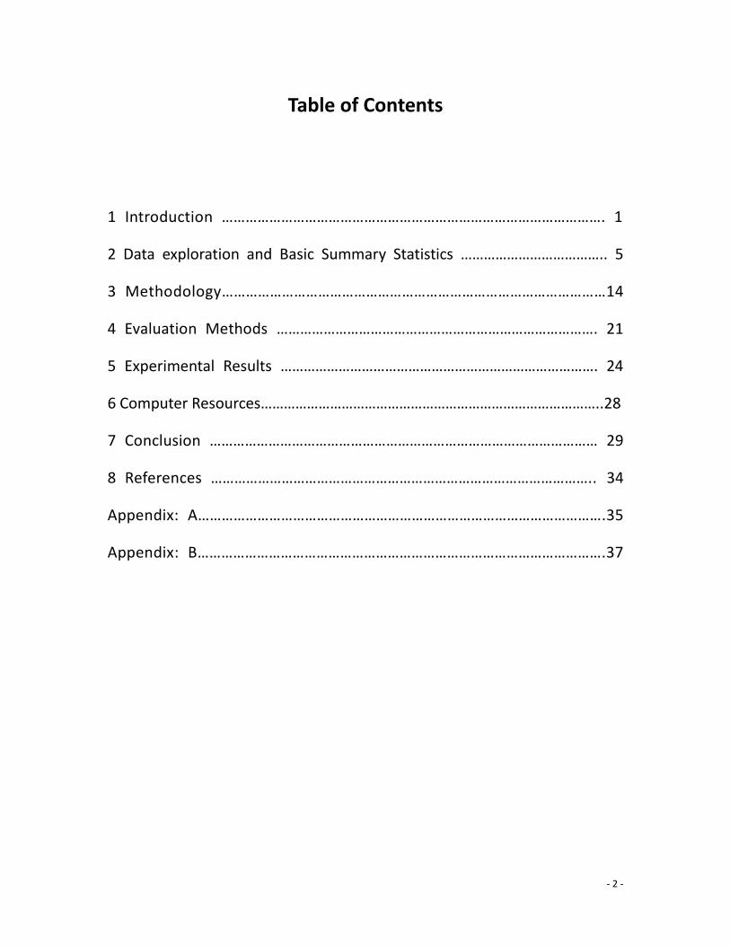
The dataset contains a substantial number of missing values for the categorical variables.

Table 2.1 shows the number and percentage of missing values. In this project, ‘missing’

was counted as a new level of the category for a categorical variable.

- 6 -

Table 2.1

Variable Name Blind_

Model

Blind

Make

Blind_

Submodel

Cat1 Cat2 Cat3 Cat4

Number of

Missing Values

8431 8431 8431 25981 4874164 3999 563164

9

Percentage of

Missing

0.064% 0.064% 0.064% 0.197% 3.697% 0.030% 42.7%

Variable Name Cat5 Cat6 Cat7 Cat8 Cat10 Cat11 Cat12

Number of

Missing Values

5637321 25981 7167634 3364 3917 31469 28882

Percentage of

Missing

42.7% 0.197% 54.4% 0.026% 0.029% 0.239% 0.219%

The Kaggle contest provided two datasets: training data and test data. Contestants could

use the training set to train their methods and the test set to compute their predictions for

contest submission. However, the insurance claim responses for the test set have never

been published. As a result, we split the training set into two sets. Observations from

2005 and 2006 were used as a training set, and observations from 2007 was used as a

test set for this project.

A basic statistics summary for the continuous variables in the original training set with

13184290 observations is shown in Appendix A. A statistics summary for categorical

variables can be found in Appendix B.

The response variable “Claim_Amount” is highly skewed with only 95,605 non-zero

values (about 0.73%) among the 13,184,290 records. A frequency histogram of the

non-zero claim amounts is shown in Figure 2.1, and of all claim amounts is shown in

Figure 2.2.

- 7 -

Figure 2.1

Figure 2.2

Histogram of Non-zero Claim_Amount

Non-zero Claim_Amount

- 8 -

Some of the other categorical covariates have a large number of levels (see Appendix B),

and this became a complication when we trying to get the statistical algorithms to work.

The correlation matrix between the continuous variables is shown in Table 2.2. There are

12 numerical predictors, named Var1 - Var8 and NVVar1 - NVVar4, and the response,

insurance claim amount. We can see some strong correlations between some of the

covariates,e.g.:Var2 and Var4. The correlation coefficients bigger than 0.7 are highlighted

in Table 2.2. However, none of the covariates is even modestly correlated with the

response.

Table 2.2

Var1 Var2 Var3 Var4 Var5 Var6 Var7

Var1 1.0000

Var2 0.5585 1.0000

Var3 0.7464 0.6457 1.0000

Var4 0.5759 0.9826 0.6570 1.0000

Var5 0.9062 0.5718 0.7861 0.5924 1.0000

Var6 0.7787 0.7722 0.8272 0.7159 0.7904 1.0000

Var7 0.6768 0.5079 0.6682 0.5201 0.4975 0.8024 1.0000

Var8 0.2689 0.7017 0.3586 0.6909 0.3020 0.5767 0.2491

NVVar1 -0.0216 -0.0198 -0.0377 -0.0196 -0.0242 -0.0386 -0.0331

NVVar2 -0.0436 -0.0524 -0.0482 -0.0533 -0.0437 -0.0566 -0.0516

NVVar3 -0.0094 -0.253 -0.0176 -0.0243 -0.0115 -0.0234 -0.0176

NVVar4 -0.0654 -0.0575 -0.0736 -0.0599 -0.0663 -0.0796 -0.0696

Claim_Amount -0.0009 -0.0013 -0.0011 -0.0012 -0.0002 -0.0013 -0.0014

Var8 NVVar1 NVVar2 NVVar3 NVVar4 Claim_Amount

Var1

Var2

Var3

Var4

Var5

Var6

Var7

Var8 1.0000

NVVar1 -0.0356 1.0000

NVVar2 -0.0427 -0.0089 1.0000

NVVar3 -0.0350 -0.0394 0.0206 1.0000

NVVar4 -0.0500 0.0762 -0.0483 -0.0433 1.0000

Claim_Amount -0.0015 0.0004 0.0014 0.0019 0.0001 1.0000

- 9 -

3.0 Methodology

Predicting the claim amount value can be regarded as a regression problem, because the

claim amount is a continuous variable. The insurance claim prediction problem could also

be considered as a classification problem by transforming the claim amount variable into

a binary variable, taking response variable as one (Y = 1) if its value is greater than zero

and zero otherwise (Y = 0). In this case, the desired outcome would be correctly

predicting whether or not there would be a claim. We considered both approaches.

Since this problem can be considered as both classification and regression, there are a

number of choices for analytical models and methods. To predict insurance claim

amounts, we tried Tweedie’s compound gamma-Poisson model, a gamma general linear

model with gamma distribution and natural log link function, and regression trees. To

classify observations as having or not having a claim, we tried logistic regression, and

classification trees. However, given the computer resources available to us, we found

that due to high dimensionality and the size of the data set, none of the algorithms used

to apply those models and methods would converge without some form of dimension

reduction.

a. Methods used to deal with high dimensionality

i. Principal Component Analysis (PCA)

Given a large set of correlated variables, principal component analysis (PCA) can be

used to summarize the pattern of variation in those variables with a smaller set of

variables called principal components (PCs). In our data set, we investigated whether the

12 continuous variables Var1-Var8 and NVVar1-NVVar4 could perhaps be adequately

represented by a smaller number of principal components.

The variation in a set of variables can be summarized by their variances and covariances.

Their PCs are a new set of variables formed by taking linear combinations of the original

variables that are uncorrelated and that explain as much variation as possible in the

fewest number of PCs. There are the same number of PCs as there are original variables.

The first PC is the normalized linear combination that has maximum variance. The

second PC is the normalized linear combination that has maximum variance among all

normalized linear combinations uncorrelated with the first PC. The third PC is the

normalized linear combination that has maximum variance among all normalized linear

combinations uncorrelated with the first two PCs, and so on. When used for dimension

reduction, the hope is that a large proportion of the total variation can be represented by a

- 10 -

relatively small number of PCs, which then substitute for the original variables. Principal

component analysis can also be used to identify meaningful underlying variables.

Another benefit of PCA is that many statistical procedures work better conceptually and

algorithmically with uncorrelated variables.

To find the principal components, we compute the covariance matrix of the data, and

calculate the eigenvalues and corresponding eigenvectors of this covariance matrix.

Then we need to normalize each eigenvector to make the set orthonormal. The

proportion of the variance that each eigenvector represents can be calculated by dividing

the eigenvalue corresponding to that eigenvector by the sum of all eigenvalues.

There are several methods to apply PCA to categorical variables, among these an

optimal scoring method due to Fisher. However, due to computational constraints, the

most feasible method for our purposes is to apply PCA to categorical variables by

establishing a design matrix that assigns dummy variables to the categorical variables.

For example, if variable Cat1 has 10 levels A to J from 1-6 individuals, the transformed

matrix will be of 6 * 10 dimension, as shown in Figure 3.1:

Figure 3.1

Original Cat1:

Transformed Cat1:

PCA is then applied to the combined set of quantitative and dummy variables.

Another method called Fisher’s optimal scoring [1] can be used to transform nominal

variables by scoring the categories. PCA could then be applied for dimension reduction

[2]. However, this method proved impractical due to its intensive use of computational

- 11 -

resources.

ii. Response Averaging

Three categorical variables with large numbers of values made fitting models and

obtaining predictions particularly challenging. These variables were Blind Make (75

values), Blind Model (1303 values), and Blind Submodel (2740 values). The approach we

used was to change the categorical values into numerical values by replacing each of

those categorical values with the average of the insurance claims in the training set

corresponding to that categorical value.

b. Classification

i. Logistic Regression

Binomial or binary logistic regression models the probability the response belongs to one

of two possible categories as a function of one or more predictors. In our case the

categories are that an insurance claim occurred (Y=1), or that an insurance claim didn’t

occur (Y=0). The logistic regression fits the model

Pr(Y = 1|X) = 𝑒𝛽𝑇

X

1+𝑒𝛽𝑇

X ,

where X is the vector of predictors.

c. Regression

i. The Tweedie Model

This dataset has a large number of zero responses, and non-zero positive responses. We

assumed that 𝑇 is the number of claims one car have and 𝑋𝑗 is the amount of the jth

claim, so the total claim for one car over the course of the year follows a Tweedie

distribution [3]. Due to its ability to simultaneously model the zeros and the continuous

positive outcomes, the Tweedie GLM is a widely used method in predicting insurance

claims.

We assume the observed response vector is Y = (𝑌1; … … . ; 𝑌𝑛)′ , where 𝑌𝑖 is distributed

as a compound gamma-Poisson distribution (Tweedie distribution) with parameters μi,

ϕ, p, if the 𝑌𝑖 are independently distributed as

- 12 -

∑ 𝑋𝑗 , 𝑇~𝑃𝑜𝑖𝑠(𝜆)

𝑇

𝑗=1

, 𝑋𝑗

~

𝐺𝑎(𝛼, 𝛾), 𝑇 ⊥ 𝑋𝑗

where Pois(λ) denotes a Poisson random variable with mean λ , and Ga(α,γ) denotes a

Gamma random variable with mean and variance equal to αγ and αγ2, respectively. As a

result, the compound Poisson distribution has a probability mass at zero accompanied by

a skewed continuous distribution on the positive real line.

The Tweedie distribution belongs to the exponential dispersion family. A two-parameter

representation of the exponential dispersion model is

𝑝(𝑦|𝜃, 𝜙) = 𝑎(𝑦, 𝜙)𝑒𝑥𝑝 (𝑦𝜃 − 𝜅(𝜃)

𝜙)

Where α and κ are known functions, θ is the natural parameter and Φ > 0 is the

dispersion parameter. For the exponential family of distributions, we have the well-known

relationships E(y) = μ=κ′(θ) and Var(y) =Φκ′′(θ). Since the mapping from θ to μ is one-to

one, κ′′(θ) can also be represented as a function of μ, denoted by V (μ) = μp in which

the value of the index parameter p lies in the interval (1, 2). By means of deriving and

equating the cumulant generating functions for the above equation, we can work out the

relationship between the two sets of parameters in the two representations as:

𝜇 = 𝜆𝛼𝛾

𝜆 =𝜇2−𝑝

𝜙(2 − 𝑝)

𝑝 =𝛼 + 2

𝛼 + 1

𝛼 =2 − 𝑝

𝑝 − 1

𝜙 =𝜆1−𝑝 ∙ (𝛼𝛾)2−𝑝

2 − 𝑝

𝜆 =𝜇2−𝑝

𝜙(2 − 𝑝)

In the Tweedie model, the mean μ= E(Y) is stipulated as a function of some linear

predictors through a link function as η(μ) = Xβ, where X is the design matrix and β is the

vector of fixed effects. For unknown p, parameter estimation can be done using the

profile likelihood approach.

There is also a zero-inflated Tweedie model, which adds additional mass at 0. The

zero-inflated Tweedie model assumes that, for the ith observation of the count data,

𝑌𝑖 is generated as below:

𝑌𝑖~ {0 with probability 𝑞𝑖

𝑇𝑤𝑒𝑒𝑑𝑖𝑒(𝜇𝑖 , 𝜙, 𝑝) with probability 1 − 𝑞𝑖

d. Decision Tree Method

A decision tree is a tree-based method that partitions the predictor space X into a set of

rectangles and fits a simple model in each one. The majority of trees use a simple

two-stage algorithm: First, partition the observations by univariate splits in a recursive

way and second, fit a model in each cell of the resulting partition. The algorithm decides

on the predictor giving the best split by doing an exhaustive search over all possible splits

and choosing the predictor and split giving the maximum of an information measure. A

tree is built recursively through this process; a process known as recursive partitioning.

Decision tree methods can be both used for classification and regression, yielding

classification and regression trees, respectively. The partitions are chosen to maximize a

measure of classification or prediction accuracy, respectively.

i. Regression Tree

A regression tree stratifies the predictor space into rectangular regions, and fits a simple

model in each of the regions to predict a continuous response.

We chose an ANOVA method similar to linear regression as the splitting criterion.

Specifically, the splitting criterion minimizes SST − (SSL + SSR), where SST =∑

(y𝑖 − y̅)2 is the sum of squares for the node, and SSR, SSL are the sums of squares for

the right and left split node, respectively.

This splitting or partitioning is then applied to each of the new branches. The process

continues until each node reaches a user-specified minimum node size and becomes a

terminal node. We then used cross-validation to prune the tree. At each pair of leaf nodes

with a common parent, we evaluated the error on the validation/testing data, and saw

whether the testing sum of squares would shrink if we removed those two nodes and

made their parent a leaf. If so, we pruned; otherwise, not. This was repeated until pruning

no longer improved the error on the testing data.

ii. The Conditional Inference Decision Tree [5][6]

However, the standard algorithm does not perform well on highly imbalanced data such

as these, due to overfitting and towards predictors with many possible splits. The

conditional inference tree algorithm nullifies this bias through the use of a significance

test procedure to screen the predictors.

Specifically, a permutation test is conducted to test the hypothesis of independence

between any of the predictors and the response. If the test fails to reject the null

hypothesis, the recursive partitioning stops. Otherwise, the predictor with strongest

association with the response is chosen and the optimal split determined. These steps

are recursively repeated until the tree is completed.

The conditional inference decision tree can both be used for classification and

regression.

e. Other models

Other models like GLM Gamma Regression, SVM, and clustering methods were also

tried to solve the problem. For GLM Gamma Regression, the original thought was to use

logistic regression first to predict whether an insurance claim would occur or not, and then

use the gamma regression to fit the non-zero responses. However, the logistic

regression’s prediction performance kept this method from being competitive, as shown

in the next section. Other methods including SVM and k-means clustering were also

implemented; however, due to the highly unbalanced nature of the data and its high

dimensionality, these methods proved impractical. Consequently, in what follows we only

provide information on models that gave a relatively good result.

4.0 Evaluation Methods - Normalized Gini Coefficient

a. Normalized Gini Coefficient

For the Kaggle contest, the specified evaluation measure is the normalized Gini

coefficient. Traditionally, statistical response models have been evaluated based on

some form of goodness of fit. Assumptions are made regarding underlying data

distributions and models are evaluated based on how well predicted values fit the

observed data values from a sample data set. Various statistical measures (Likelihood,

𝑅2, the F statistic, the Chi Square statistic, classification indices and so on) are used to

evaluate or produce the goodness of fit. In the insurance claim prediction, the Kaggle

contest required the contestants to use the normalized Gini coefficient as the evaluation

measure.

To define the normalized Gini coefficient, we first need to define Lorenz curve: “Let

p∈ [0,100], and define the function L(p)to be the proportion of all claims associated with

the largest p percent of predicted values. The graph of L(p) versus p is the Lorenz

curve. The line at 45 degrees represents the results expected from a “null model”, that is,

from predicting by randomly choosing a claim amount from the data set, so the area

between L(p) and the 45 degree line represents the improvement of the prediction

method over chance prediction.. Let L1(p) denote the Lorenz curve for the prediction

method being evaluated and L2(p) the Lorenz curve for perfect prediction, and let A1 and

A2 be the respective areas between the Lorenz curves and the 45 degree line.. The

normalized Gini coefficient is the ratio A1/A2.

As a result of this definition, the actual predicted values do not matter for evaluating the

normalized Gini coefficient, only the relative ordering of these predictions does.

b. Confusion Matrix

The confusion matrix, also known as the contingency table, is a specific table layout that

displays the performance of a classification test. For a binary classification it contains two

rows and two columns that report the number of false positives (FP), false negatives (FN),

true positives (TP), and true negatives (TN) (Table 4.1).

Table 4.1

Model Prediction

Positive

Model Prediction

Negative

Truth: Positive TP FN

Truth: Negative FP TN

5.0 Experimental Results

The original training set has information from years 2005 to 2007, with 13184290

observations. In the Kaggle contest, participants developed their predictors using the

training data, and used them to predict claims in the test set. They submitted these

predictions and the sponsors evaluated the results using the normalized Gini coefficient.

The claims data in the test set were never published, so we cannot evaluate our

predictors on that data. However, the leader board scoring can be found on the Kaggle

website and shows how the best prediction methods (which were also not disclosed)

performed on the test data.

While we don’t have the test set claims data, we can assess the similarity of the

covariates in my test set (Table 5.1) and the Kaggle test sets (Table 5.2).

Table 5.1

Name Mean SD Min Max

Var1 0.01759 0.9849655 -2.57822 5.14339

Var2 0.01301 0.9957419 -2.49339 7.82942

Var3 0.01553 1.009001 -2.79033 5.56322

Var4 0.02049 0.995602 -2.50822 7.58926

Var5 0.02844 0.9944316 -3.35034 4.01817

Var6 0.008497 0.9910882 -2.376657 4.584289

Var7 0.008933 1.001785 -2.778491 4.127148

Var8 0.00117 1.025582 -2.16304 47.35072

NVVar1 -0.009784 1.02622 -0.23153 6.627110

NVVar2 0.01242 1.035767 -0.26612 8.88308

NVVar3 -0.01515 1.042242 -0.27234 8.69114

NVVar4 0.005654 1.015079 -0.25142 6.388802

Table 5.2

Name Mean SD Min Max

Var1 -0.29122 0.44803 -2.57822 3.08644

Var2 -0.05289 0.898978 -2.14757 7.82942

Var3 -0.2088 0.692303 -2.4664 2.0691

Var4 -0.08893 0.881487 -2.16994 7.94445

Var5 -0.1727 0.615788 -5.0572 2.8763

Var6 -0.37134 0.55005 -2.02925 2.85897

Var7 -0.5528 0.502969 -2.2133 1.6819

Var8 0.08771 1.095868 -1.4848 46.72172

NVVar1 -0.02708 0.930115 -0.23153 6.62711

NVVar2 -0.01003 0.984403 -0.26612 8.88308

NVVar3 -0.04531 0.895811 -0.27234 8.69114

NVVar4 0.009567 1.042618 -0.25142 6.3888

We can see that given the large samples, the continuous covariates Var1, Var3, Var6 and

Var7 in the training set and test set have some significant differences (highlighted in

yellow). For the other continuous variables, the mean and standard deviations are close,

and the maximum and minimum values for all variables are very close. While these

summary statistics do not rule out the possibility that similar results would be obtained by

using our methods on the Kaggle test data, they do indicate the possibility of substantial

differences due to differences in the distributions of the covariates in the two sets, .

We further checked the correlation matrix of our test set (Table 5.3) and the Kaggle test

set (Table 5.4)

Table 5.3

Var1 Var2 Var3 Var4 Var5 Var6

Var1 1.0000

Var2 0.5582 1.0000

Var3 0.7488 0.6491 1.0000

Var4 0.5795 0.9837 0.6623 1.0000

Var5 0.9112 0.5691 0.7876 0.5925 1.0000

Var6 0.7800 0.7700 0.8332 0.7867 0.7530 1.0000

Var7 0.6770 0.5064 0.6762 0.5215 0.5100 0.8066

Var8 0.2682 0.6999 0.3641 0.6898 0.2976 0.5714

NVVar1 -0.0197 -0.0191 -0.0356 -0.0188 -0.0222 -0.0367

NVVar2 -0.0444 -0.0529 -0.0494 -0.0538 -0.0443 -0.0569

NVvar3 -0.0107 -0.0274 -0.0201 -0.0264 -0.0124 -0.0252

NVVar4 -0.0631 -0.0561 -0.0704 -0.0583 -0.0637 -0.0761

Var7 Var8 NVVar1 NVVar2 NVVar3 NVVar4

Var1

Var2

Var3

Var4

Var5

Var6

Var7 1.0000

Var8 0.2462 1.0000

NVVar1 -0.0331 -0.0337 1.0000

NVVar2 -0.0520 -0.0418 -0.0106 1.0000

NVvar3 -0.0200 -0.0348 -0.0381 0.0192 1.0000

NVVar4 -0.0680 -0.4830 0.0675 -0.0454 -0.0414 1.0000

Table 5.4

Var1 Var2 Var3 Var4 Var5 Var6

Var1 1.0000

Var2 0.4568 1.0000

Var3 0.8403 0.4851 1.0000

Var4 0.5485 0.9964 0.4915 1.0000

Var5 0.8236 0.4744 0.7947 0.4809 1.0000

Var6 0.8504 0.6873 0.8503 0.6912 0.7309 1.0000

Var7 0.5480 0.0601 0.5585 0.0643 0.2422 0.5168

Var8 0.3623 0.7328 0.3128 0.7321 0.2805 0.5798

NVVar1 -0.0439 -0.0201 -0.0503 -0.0205 -0.0358 -0.0510

NVVar2 -0.0478 -0.0556 -0.0527 -0.0556 -0.0463 -0.0596

NVvar3 -0.0269 -0.0183 -0.0181 -0.0183 -0.0144 -0.0207

NVVar4 --0.0726 -0.0705 -0.0827 -0.0709 -0.0646 -0.0936

Var7 Var8 NVVar1 NVVar2 NVVar3 NVVar4

Var1

Var2

Var3

Var4

Var5

Var6

Var7 1.0000

Var8 -0.0677 1.0000

NVVar1 -0.0471 -0.0275 1.0000

NVVar2 -0.0243 -0.0429 -0.0092 1.0000

NVvar3 -0.0133 -0.0153 0.0284 0.0284 1.0000

NVVar4 -0.0532 -0.0652 -0.0396 -0.0396 -0.0334 1.0000

To better compare the above tables, we subtracted the Table 5.4 entries from the

corresponding entries in Table 5.3. The results are shown in Table 5.5.

Table 5.5

Var1 Var2 Var3 Var4 Var5 Var6

Var1 0

Var2 0.1014 0

Var3 -0.0915 0.164 0

Var4 0.031 -0.0127 0.1708 0

Var5 0.0876 0.0947 -0.0071 0.1116 0

Var6 -0.0704 0.0827 -0.0171 0.0955 0.0221 0

Var7 0.129 0.4463 0.1177 0.4572 0.2678 0.2898

Var8 -0.0941 -0.0329 0.0513 -0.0423 0.0171 -0.0084

NVVar1 0.0242 0.001 0.0147 0.0017 0.0136 0.0143

NVVar2 0.0034 0.0027 0.0033 0.0018 0.002 0.0027

NVvar3 0.0162 -0.0091 -0.002 -0.0081 0.002 -0.0045

NVVar4 -0.1357 0.0144 0.0123 0.0126 0.0009 0.0175

Var7 Var8 NVVar1 NVVar2 NVVar3 NVVar4

Var1

Var2

Var3

Var4

Var5

Var6

Var7 0

Var8 0.3139 0

NVVar1 0.014 -0.0062 0

NVVar2 -0.0277 0.0011 -0.0014 0

NVvar3 -0.0067 -0.0195 -0.0665 -0.0092 0

NVVar4 -0.0148 -0.4178 0.1071 -0.0058 -0.008 0

We can see that for most variables, the correlation coefficients are very close, except for

variable Var7. The differences in the correlation coefficients of Var7 with Var2, Var4, Var5,

Var6 and Var8 are bigger than 0.2.

Since we don't have the response on the Kaggle test set, in order to evaluate the

performance of the various methods considered, we divided the original training set into a

training and a test set. The training set contains information from 2005 to 2006 with

8473402 (64%) observations, and the test set contains information from 2007 with

4710888 (36%) observations. We trained our predictors on this training set and tested

them on this test set, in the hope is that the results would be similar to what we would

have obtained if we had applied them to the true test set. In what follows, “training set”

and “test set” will refer to these two sets.

One question is the similarity of the training set and test set. To check this, we created

summary statistics for some of the variables in the training and test sets. For the

response variable Claim_Amount, the summary statistics of non-zero and zero values are

shown in Table 5.6. The histogram of non-zero values in the training set is shown in

Figure 5.1 and some summary statistics are shown in Table 5.7. The corresponding

displays for the test set are shown in Figure 5.2 and Table 5.8.

Table 5.6 Comparison of Zero and Non-Zero Values

Counts of non-zero values Counts of -zero values Percentage of none-zero values

Training Set 61838 8411564 0.735%

Test Set 33767 4677121 0.722%

Figure 5.1

Table 5.7 Summary Statistics, Training Set

Non-zero Claim

Amount

mean Standard

deviation

min max

201.00 465.2236 0.00 11440.00

Histogram of Non-zero Claim_Amount, Training Set

Non-zero Claim_Amount

Figure 5.2

Table 5.8 Summary Statistics, Test Set

Non-zero Claim

Amount

mean Standard

deviation

min max

163.20 312.5247 0.00 7667.00

We can see is that the percentage of zero and non-zero values are similar in the training

set and test set, but the summary statistics of non-zero values are not as similar.

Essentially, there are substantial differences between our test set and Kaggle’s and

between our training and test set.

a. Logistic Regression

Logistic regression can be used to classify according to whether or not an insurance

Histogram of Non-zero Claim_Amount, Test Set

Non-zero Claim_Amount

claim occurred. However, 162G of memory are needed to fit a logistic regression with all

available predictor variables, which is not available on our computing cluster. So we first

tried to delete the two variables that have over 1000 levels each: Blind_Model and

Blind_Submodel.

In the logistic regression, we set the response equal to 1 for any positive claim amount.

The result of fitting the logistic regression on the test set is shown in Table 5.9.

Table 5.9 Confusion Matrix

Real value \ Prediction Positive Negative

Truth: positive 4643325 33183

Truth: negative 33796 584

We can see the prediction is not good. From the above, we can see the model fails to

predict non-zeros.

We then tried to use response averaging to transform the three categorical variables

Blind_Make, Blind_Model and Blind_Submodel into numerical values, and then fitted the

logistic regression. The result is shown in Table 5.10

Table 5.10 Confusion Matrix with Response Averaging

Real value \ Prediction Positive Negative

Truth: positive 4643293 33215

Truth: negative 33828 552

We can see that by using response averaging the result is worse than the previous

logistic regression model. We further tried using PCA and response averaging as

predictors, the result is shown in Table 5.11

Table 5.11 Confusion Matrix with Response Averaging and PCA

Real value \ Prediction Positive Negative

Truth: positive 4643272 33236

Truth: negative 33849 531

From Table 5.11 we can see the result is worse than the other two. In this case, response

averaging and PCA doesn’t help improving the prediction accuracy, on the contrary, they

make it worse.

b. Tweedie Model with Sampling Subset

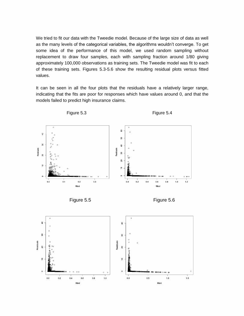
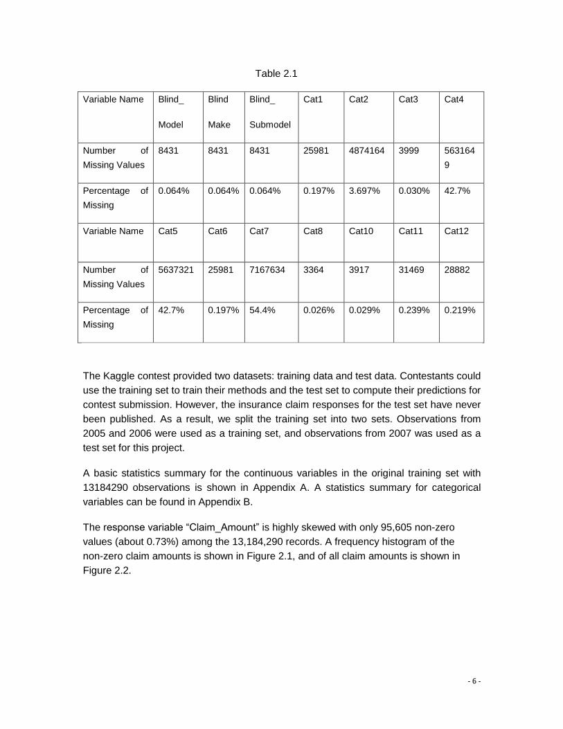
We tried to fit our data with the Tweedie model. Because of the large size of data as well

as the many levels of the categorical variables, the algorithms wouldn’t converge. To get

some idea of the performance of this model, we used random sampling without

replacement to draw four samples, each with sampling fraction around 1/80 giving

approximately 100,000 observations as training sets. The Tweedie model was fit to each

of these training sets. Figures 5.3-5.6 show the resulting residual plots versus fitted

values.

It can be seen in all the four plots that the residuals have a relatively larger range,

indicating that the fits are poor for responses which have values around 0, and that the

models failed to predict high insurance claims.

Figure 5.3 Figure 5.4

Figure 5.5 Figure 5.6

We took two samples (sample_trainB, sample_trainC) among the four samples above to

calculate the normalized Gini coefficient and get 0.38 for sample_trainB and 0.39 for

sample_trainC. However, applying the model trained on training sample trainB to predict

the responses for sample trainC, resulted in a normalized Gini coefficient of only

0.004039204.

Because the algorithm failed to converge for the full data set, we needed to find a way to

deal with the high dimensionality problem. Our first attempted solution was to use PCA to

reduce the dimension of the predictor space.

c. PCA

To apply PCA to the categorical variables, we first transformed them to dummy variables

as described in the methodology section. Taking all the resulting the variables,

continuous and categorical, we find that 38 principal components account for 98% of the

variation. Fitting the Tweedie model to the training data with these as predictors, we

obtain a normalized Gini coefficient on the test set, 0.02249483. The resulting residual

plot is shown in Figure 5.7:

Figure 5.7

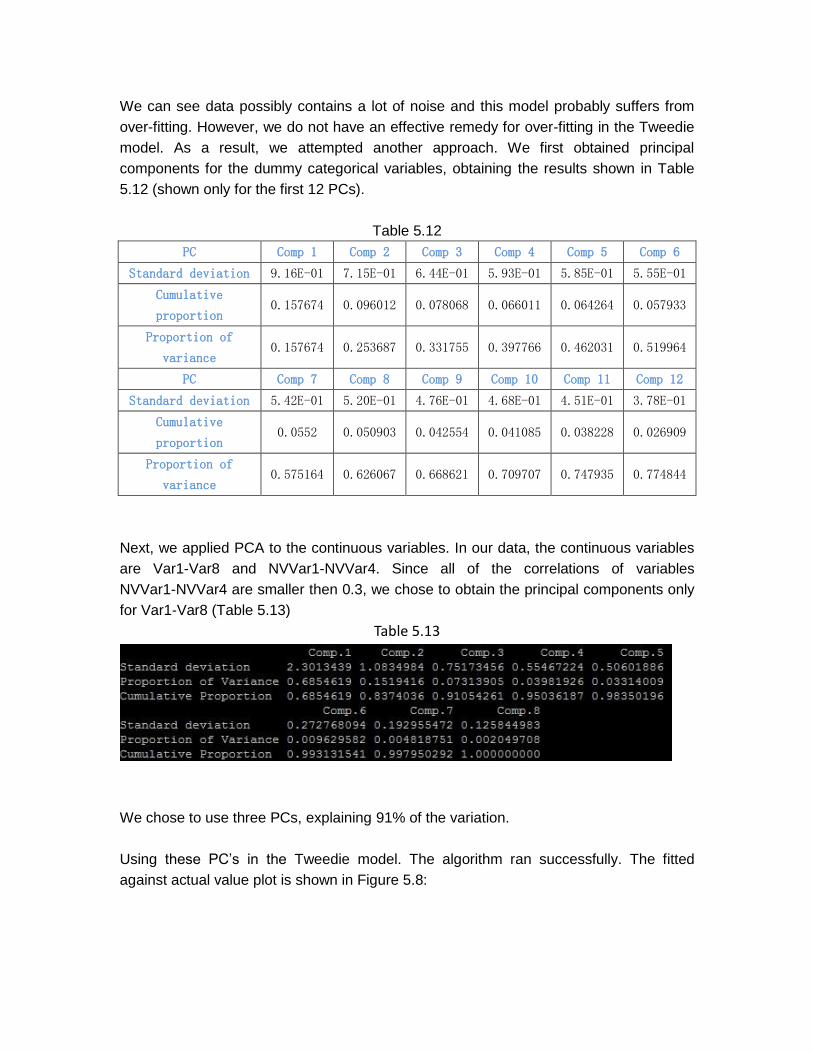
We can see data possibly contains a lot of noise and this model probably suffers from

over-fitting. However, we do not have an effective remedy for over-fitting in the Tweedie

model. As a result, we attempted another approach. We first obtained principal

components for the dummy categorical variables, obtaining the results shown in Table

5.12 (shown only for the first 12 PCs).

Table 5.12

PC Comp 1 Comp 2 Comp 3 Comp 4 Comp 5 Comp 6

Standard deviation 9.16E-01 7.15E-01 6.44E-01 5.93E-01 5.85E-01 5.55E-01

Cumulative

proportion 0.157674 0.096012 0.078068 0.066011 0.064264 0.057933

Proportion of

variance 0.157674 0.253687 0.331755 0.397766 0.462031 0.519964

PC Comp 7 Comp 8 Comp 9 Comp 10 Comp 11 Comp 12

Standard deviation 5.42E-01 5.20E-01 4.76E-01 4.68E-01 4.51E-01 3.78E-01

Cumulative

proportion 0.0552 0.050903 0.042554 0.041085 0.038228 0.026909

Proportion of

variance 0.575164 0.626067 0.668621 0.709707 0.747935 0.774844

Next, we applied PCA to the continuous variables. In our data, the continuous variables

are Var1-Var8 and NVVar1-NVVar4. Since all of the correlations of variables

NVVar1-NVVar4 are smaller then 0.3, we chose to obtain the principal components only

for Var1-Var8 (Table 5.13)

Table 5.13

We chose to use three PCs, explaining 91% of the variation.

Using these PC’s in the Tweedie model. The algorithm ran successfully. The fitted

against actual value plot is shown in Figure 5.8:

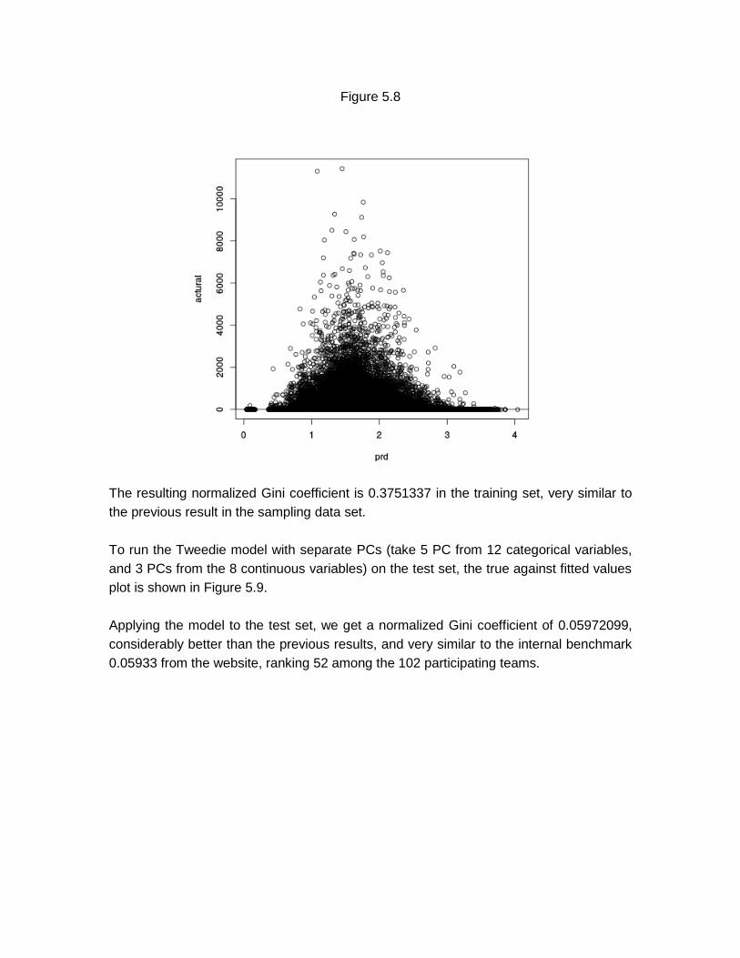
Figure 5.8

The resulting normalized Gini coefficient is 0.3751337 in the training set, very similar to

the previous result in the sampling data set.

To run the Tweedie model with separate PCs (take 5 PC from 12 categorical variables,

and 3 PCs from the 8 continuous variables) on the test set, the true against fitted values

plot is shown in Figure 5.9.

Applying the model to the test set, we get a normalized Gini coefficient of 0.05972099,

considerably better than the previous results, and very similar to the internal benchmark

0.05933 from the website, ranking 52 among the 102 participating teams.

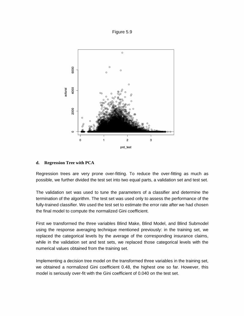
Figure 5.9

d. Regression Tree with PCA

Regression trees are very prone over-fitting. To reduce the over-fitting as much as

possible, we further divided the test set into two equal parts, a validation set and test set.

The validation set was used to tune the parameters of a classifier and determine the

termination of the algorithm. The test set was used only to assess the performance of the

fully-trained classifier. We used the test set to estimate the error rate after we had chosen

the final model to compute the normalized Gini coefficient.

First we transformed the three variables Blind Make, Blind Model, and Blind Submodel

using the response averaging technique mentioned previously: in the training set, we

replaced the categorical levels by the average of the corresponding insurance claims,

while in the validation set and test sets, we replaced those categorical levels with the

numerical values obtained from the training set.

Implementing a decision tree model on the transformed three variables in the training set,

we obtained a normalized Gini coefficient 0.48, the highest one so far. However, this

model is seriously over-fit with the Gini coefficient of 0.040 on the test set.

As we did for the Tweedie model, we used PCA to transform the 12 categorical variables

Cat1- -Cat12 (using the design matrix set-up), and as before took 5 PCs with 46% of their

total variance and among the 8 continuous variables Var1-Var8, we took 3 PC’s with 91%

of their total variance.

Finally, we implemented the decision tree model with the PCs from PCA as the predictors,

and pruned the tree using ten-fold cross-validation. The final model is shown in Figure

5.10 and 5.11

Figure 5.10

Figure 5.11

The variable new_valueaa is the variable transformed from the original variable

Blind_Submodel which has over 2000 levels and is the least granular of the car model

descriptors. We can see this is the most important variable in the decision tree. By using

the model above, the normalized Gini coefficient on the training set is 0.152567, and on

the test set is 0.080135, which, if it applied to the Kaggle test data, would rank 27th

among contest results.

e. Conditional Inference Tree with PCA

As mentioned in the methodology section, a conditional inference method for tree fitting

was developed to deal with highly imbalanced data, such as ours.

The covariates used were the same as it is for the Regression Tree. Since this method

can both be used for regression and decision trees, we first tried the decision tree for

classification.

We can see from the resulting decision tree in Figure 5.12, the top three important

predictor variables are: NVCat, Model_Year, and new-valueaa (the sub_model

transformed by the response averaging method).

Figure 5.12

And the confusion matrix for the prediction evaluation is shown below in Table 5.14

Table 5.14

Real value \ Prediction Positive Negative

Truth: positive 4643310 33198

Truth: negative 33852 528

This result is worse than all the results from logistic regression; the conditional inference

classification tree notably fails to identify nonzero claims.

We then tried the conditional inference regression tree, and the covariates used are the

same as for the classification tree. The tree model is shown as below in Figure 5.13:

Figure 5.13

The final normalized Gini coefficient of the conditional inference regression tree on the

test set is 0.06190335, which, if it applied to the Kaggle test data, would rank 47th among

contest results.

Comparing the result of Gini coefficient obtained by regression tree using different fitting

method, the traditional regression tree performs better for our data set. The decision

tree’s result is worse than logistic regression model.

6.0 Computer Resources

All the models were run using R on a linux cluster, which contains two Intel E5-2670

2.60Ghz 20M Cache 8-Core 115W Processor, with 378 GB of shared memory used by

other people, and we were not able to access all the 378 GB memory.

The cluster we used doesn’t support parallel computing, so it takes long time to run most

of the models.

7.0 Conclusion

The aim of this project was to compare the performances of various statistical models

and methods on predicting the bodily injury liability insurance claim payments based on

the characteristics of the insured’s vehicles in a particular data set, which was used in a

Kaggle data competition. We tried a number of methods, including principal component

analysis, response averaging, the Tweedie model, and decision tree methods. The most

successful methods, based on the normalized Gini coefficient, were regression tree with

PCA, which on our test set gave a value of 0.080135. If our test set were comparable to

the test set in the competition (a questionable assumption), our results would have

earned 27th in the ranking. We also tried viewing the problem as classification, using

logistic regression and classification trees to see how well these methods could predict

whether a car will have insurance claim or not. The evaluation method for classification is

the confusion matrix. Classification trees performed worse than logistic regression for this

data.

One difficulty we faced was not knowing the exact values of many of the predictor

variables, as these had been anonymized. This prevented us from making some

informed choices we might have made in the presence of full information.

Another difficulty in predicting insurance claims using only the predictors given, is that

many other factors contribute to the frequency and severity of car accidents including

how, where and under what conditions people drive, as well as what cars they are driving.

But the most important influential predictors are actually related to the drivers, including

their driving history, driving behavior, etc. Therefore, prediction only based on the car

characteristics is almost an impossible mission, and the best predictions we could make

were not particularly accurate, if the criterion were the difference between the prediction

and the actual claim. Indeed, in this case, a not unreasonable strategy would be to

predict a claim amount of 0 for all cases, since more than 99% of all claims are 0. In fact,

in terms of classification, this strategy proved better than both the classification tree and

logistic regression methods.

However, using the normalized Gini coefficient, which uses only the rankings of the

predictions, as the measure of prediction quality, we were able to obtain respectable

results as measured by the best contest entries.

Another challenging part of the project was to find a way to process the data and create a

data set that could be used by the algorithms. Not all the algorithms are able to handle

the presence of categorical variables, so those variables have to be transformed into

numerical variables. Furthermore, transforming categorical variables that have over 2000

levels is even more difficult. From all the models we tried, PCA combined with

Regression Tree has the best result. Although the Tweedie model is famous for the

insurance claim prediction problem, the regression tree gave the most accurate result in

this insurance claim prediction project.

Among the several methods we have tried, the regression tree algorithm has been

proven the most efficient model for prediction given existing and limited resources.

However, grid search has been identified as a method to find out the best settings of

parameters for a decision tree analysis. As part of the future work, it might be beneficial to

implement this method using parallel computing to better tune the parameters of the

regression tree.

Reference

[1] Ronald Fisher,Transform Nominal Variables by Optimally Scoring the Categories.

1938

[2] J. C. Gower Fisher's Optimal Scores and Multiple Correspondence Analysis

Biometrics Vol. 46, No. 4. Dec.1990, pp. 947-961

[3] Peter K Dunn, Gordon K. Smyth. Evaluation of Tweedie exponential dispersion model

densities by Fourier inversion. 2007.

[4] Gareth James, Daniela Witten, Trevor Hastie, Robert Tibshirani. An Introduction to

Statistical Learning: with Applications in R (Springer Texts in Statistics) Published by

Springer .2013

[5] Torsten Hothorn,. Kurt Hornik, and Achim Zeileis. Unbiased Recursive Partitioning: A

Conditional Inference Framework. Journal of Computational and Graphical Statistics,

[6] Terry M. Therneau, Elizabeth J. Atkinson, Mayo Foundation, An Introduction to

Recursive Partitioning Using the RPART Routines, March 28 2014

[7] Chao-Tung Yang, Shu-Tzu Tsai, Kuan-Ching Li, Decision Tree Construction for Data

Mining on Grid Computing Environments. March 2005

[8]George Deltas (February 2003). "The Small-Sample Bias of the Gini Coefficient:

Results and Implications for Empirical Research". The Review of Economics and

Statistics 85(1): 226–234

Appendix A

Statistics Summary for Numerical Variables:

Name Mean Standard Deviation Min MaxVar1          -0.01011925 9.800609e-01   -2.5782218   5.143392e+00Var2          -0.06508703 9.684165e-01   -2.4933927  7.829420e+00Var3          -0.02543391 1.018902e+00   -2.7903352  5.563325e+00Var4          -0.05456793 9.680170e-01   -2.5082161  7.589262e+00Var5           0.003838594 9.910490e-01   -3.3503442  4.018167e+00Var6          -0.04012272 9.792078e-01   -2.3766568  4.584289e+00Var7          -0.02421288 1.006433e+00   -2.7784905  4.127148e+00Var8          -0.05856059 1.003954e+00   -2.1630421  4.735074e+01NVVar1         0.01468409 1.031040e+00   -0.2315299  6.627110e+00NVVar2         0.01751169 1.038212e+00   -0.2661168  8.883081e+00NVVar3         0.01354226 1.027748e+00   -0.2723372  8.691144e+00NVVar4         0.01851377 1.034274e+00   -0.2514189  6.388803e+00Claim_Amount   1.360658 3.900103e+01    0  1.144075e+04

Appendix B

Variable Name Category Counts Examples and Counts

Blind_Make 75 K: 1657185,

Q 233255

AR 202083

D 174362

……

Blind_Model 1303 A.1, A.2,…,A.15,…,B.1,…

Blind_Submodel 2740 A.1.1,…,B.2.0,…,D.5.2,…

Cat1 11 D 2487951

B 4017739

J 233968

G 782602

……

Cat2

4 C 5895027

? 4874164

A 2191054

B 224045

Cat 3 7 F 872031

A 7488029

B 2256802

……

Cat 4 4 ? 5631649

A 5723163

C 1454425

B 375053

……

Cat 5 4 ? 5637321

A 6683980

C 779280

B 83709

……

Cat 6 6 C 3677694

E 1173316

? 25981

……

Cat 7 5 ? 7167634

C 4618653

A 1050621

……

Cat 8 4 C 880481

A 8626513

B 3673932

? 3364

Cat 9 2 A 2333508

B 10850782

Cat 10 4 B 3969170

A 8573092

C 638111

? 3917

Cat 11

7

F 787998

B 3174528

E 816595

……

Cat 12 6 D 3525723

B 4348276

C 3619974

……

OrdCat 8 4 5935475

5 2964704

2 4146321

……

NVCat 15 M 5767944

O 3416948

F 325556

……