Embed Size (px)
Citation preview


Data MiningThird Edition

The Morgan Kaufmann Series in Data Management Systems (Selected Titles)
Joe Celko’s Data, Measurements, and Standards in SQLJoe Celko
Information Modeling and Relational Databases, 2nd EditionTerry Halpin, Tony Morgan
Joe Celko’s Thinking in SetsJoe Celko
Business MetadataBill Inmon, Bonnie O’Neil, Lowell Fryman
Unleashing Web 2.0Gottfried Vossen, Stephan Hagemann
Enterprise Knowledge ManagementDavid Loshin
The Practitioner’s Guide to Data Quality ImprovementDavid Loshin
Business Process Change, 2nd EditionPaul Harmon
IT Manager’s Handbook, 2nd EditionBill Holtsnider, Brian Jaffe
Joe Celko’s Puzzles and Answers, 2nd EditionJoe Celko
Architecture and Patterns for IT Service Management, 2nd Edition, Resource Planningand GovernanceCharles Betz
Joe Celko’s Analytics and OLAP in SQLJoe Celko
Data Preparation for Data Mining Using SASMamdouh Refaat
Querying XML: XQuery, XPath, and SQL/ XML in ContextJim Melton, Stephen Buxton
Data Mining: Concepts and Techniques, 3rd EditionJiawei Han, Micheline Kamber, Jian Pei
Database Modeling and Design: Logical Design, 5th EditionToby J. Teorey, Sam S. Lightstone, Thomas P. Nadeau, H. V. Jagadish
Foundations of Multidimensional and Metric Data StructuresHanan Samet
Joe Celko’s SQL for Smarties: Advanced SQL Programming, 4th EditionJoe Celko
Moving Objects DatabasesRalf Hartmut Guting, Markus Schneider
Joe Celko’s SQL Programming StyleJoe Celko
Fuzzy Modeling and Genetic Algorithms for Data Mining and ExplorationEarl Cox

Data Modeling Essentials, 3rd EditionGraeme C. Simsion, Graham C. Witt
Developing High Quality Data ModelsMatthew West
Location-Based ServicesJochen Schiller, Agnes Voisard
Managing Time in Relational Databases: How to Design, Update, and Query Temporal DataTom Johnston, Randall Weis
Database Modeling with Microsoft R© Visio for Enterprise ArchitectsTerry Halpin, Ken Evans, Patrick Hallock, Bill Maclean
Designing Data-Intensive Web ApplicationsStephano Ceri, Piero Fraternali, Aldo Bongio, Marco Brambilla, Sara Comai, Maristella Matera
Mining the Web: Discovering Knowledge from Hypertext DataSoumen Chakrabarti
Advanced SQL: 1999—Understanding Object-Relational and Other Advanced FeaturesJim Melton
Database Tuning: Principles, Experiments, and Troubleshooting TechniquesDennis Shasha, Philippe Bonnet
SQL: 1999—Understanding Relational Language ComponentsJim Melton, Alan R. Simon
Information Visualization in Data Mining and Knowledge DiscoveryEdited by Usama Fayyad, Georges G. Grinstein, Andreas Wierse
Transactional Information SystemsGerhard Weikum, Gottfried Vossen
Spatial DatabasesPhilippe Rigaux, Michel Scholl, and Agnes Voisard
Managing Reference Data in Enterprise DatabasesMalcolm Chisholm
Understanding SQL and Java TogetherJim Melton, Andrew Eisenberg
Database: Principles, Programming, and Performance, 2nd EditionPatrick and Elizabeth O’Neil
The Object Data StandardEdited by R. G. G. Cattell, Douglas Barry
Data on the Web: From Relations to Semistructured Data and XMLSerge Abiteboul, Peter Buneman, Dan Suciu
Data Mining: Practical Machine Learning Tools and Techniques with Java Implementations,3rd EditionIan Witten, Eibe Frank, Mark A. Hall
Joe Celko’s Data and Databases: Concepts in PracticeJoe Celko
Developing Time-Oriented Database Applications in SQLRichard T. Snodgrass
Web Farming for the Data WarehouseRichard D. Hackathorn

Management of Heterogeneous and Autonomous Database SystemsEdited by Ahmed Elmagarmid, Marek Rusinkiewicz, Amit Sheth
Object-Relational DBMSs, 2nd EditionMichael Stonebraker, Paul Brown, with Dorothy Moore
Universal Database Management: A Guide to Object/Relational TechnologyCynthia Maro Saracco
Readings in Database Systems, 3rd EditionEdited by Michael Stonebraker, Joseph M. Hellerstein
Understanding SQL’s Stored Procedures: A Complete Guide to SQL/PSMJim Melton
Principles of Multimedia Database SystemsV. S. Subrahmanian
Principles of Database Query Processing for Advanced ApplicationsClement T. Yu, Weiyi Meng
Advanced Database SystemsCarlo Zaniolo, Stefano Ceri, Christos Faloutsos, Richard T. Snodgrass, V. S. Subrahmanian,Roberto Zicari
Principles of Transaction Processing, 2nd EditionPhilip A. Bernstein, Eric Newcomer
Using the New DB2: IBM’s Object-Relational Database SystemDon Chamberlin
Distributed AlgorithmsNancy A. Lynch
Active Database Systems: Triggers and Rules for Advanced Database ProcessingEdited by Jennifer Widom, Stefano Ceri
Migrating Legacy Systems: Gateways, Interfaces, and the Incremental ApproachMichael L. Brodie, Michael Stonebraker
Atomic TransactionsNancy Lynch, Michael Merritt, William Weihl, Alan Fekete
Query Processing for Advanced Database SystemsEdited by Johann Christoph Freytag, David Maier, Gottfried Vossen
Transaction ProcessingJim Gray, Andreas Reuter
Database Transaction Models for Advanced ApplicationsEdited by Ahmed K. Elmagarmid
A Guide to Developing Client/Server SQL ApplicationsSetrag Khoshafian, Arvola Chan, Anna Wong, Harry K. T. Wong

Data MiningConcepts and Techniques
Third Edition
Jiawei HanUniversity of Illinois at Urbana–Champaign
Micheline KamberJian Pei
Simon Fraser University
AMSTERDAM • BOSTON • HEIDELBERG • LONDONNEW YORK • OXFORD • PARIS • SAN DIEGO
SAN FRANCISCO • SINGAPORE • SYDNEY • TOKYO
Morgan Kaufmann is an imprint of Elsevier

Morgan Kaufmann Publishers is an imprint of Elsevier.225 Wyman Street, Waltham, MA 02451, USA
c© 2012 by Elsevier Inc. All rights reserved.
No part of this publication may be reproduced or transmitted in any form or by any means,electronic or mechanical, including photocopying, recording, or any information storage andretrieval system, without permission in writing from the publisher. Details on how to seekpermission, further information about the Publisher’s permissions policies and ourarrangements with organizations such as the Copyright Clearance Center and the CopyrightLicensing Agency, can be found at our website: www.elsevier.com/permissions.
This book and the individual contributions contained in it are protected under copyright bythe Publisher (other than as may be noted herein).
Notices
Knowledge and best practice in this field are constantly changing. As new research andexperience broaden our understanding, changes in research methods or professional practices,may become necessary. Practitioners and researchers must always rely on their own experienceand knowledge in evaluating and using any information or methods described herein. In usingsuch information or methods they should be mindful of their own safety and the safety of others,including parties for whom they have a professional responsibility.
To the fullest extent of the law, neither the Publisher nor the authors, contributors, or editors,assume any liability for any injury and/or damage to persons or property as a matter of productsliability, negligence or otherwise, or from any use or operation of any methods, products,instructions, or ideas contained in the material herein.
Library of Congress Cataloging-in-Publication Data
Han, Jiawei.Data mining : concepts and techniques / Jiawei Han, Micheline Kamber, Jian Pei. – 3rd ed.
p. cm.ISBN 978-0-12-381479-1
1. Data mining. I. Kamber, Micheline. II. Pei, Jian. III. Title.QA76.9.D343H36 2011006.3′12–dc22 2011010635
British Library Cataloguing-in-Publication DataA catalogue record for this book is available from the British Library.
For information on all Morgan Kaufmann publications, visit ourWeb site at www.mkp.com or www.elsevierdirect.com
Printed in the United States of America11 12 13 14 15 10 9 8 7 6 5 4 3 2 1

To Y. Dora and Lawrence for your love and encouragement
J.H.
To Erik, Kevan, Kian, and Mikael for your love and inspiration
M.K.
To my wife, Jennifer, and daughter, Jacqueline
J.P.

This page intentionally left blank

Contents
Foreword xix
Foreword to Second Edition xxi
Preface xxiii
Acknowledgments xxxi
About the Authors xxxv
Chapter 1 Introduction 1
1.1 Why Data Mining? 11.1.1 Moving toward the Information Age 11.1.2 Data Mining as the Evolution of Information Technology 2
1.2 What Is Data Mining? 5
1.3 What Kinds of Data Can Be Mined? 81.3.1 Database Data 91.3.2 Data Warehouses 101.3.3 Transactional Data 131.3.4 Other Kinds of Data 14
1.4 What Kinds of Patterns Can Be Mined? 151.4.1 Class/Concept Description: Characterization and Discrimination 151.4.2 Mining Frequent Patterns, Associations, and Correlations 171.4.3 Classification and Regression for Predictive Analysis 181.4.4 Cluster Analysis 191.4.5 Outlier Analysis 201.4.6 Are All Patterns Interesting? 21
1.5 Which Technologies Are Used? 231.5.1 Statistics 231.5.2 Machine Learning 241.5.3 Database Systems and Data Warehouses 261.5.4 Information Retrieval 26
ix

x Contents
1.6 Which Kinds of Applications Are Targeted? 271.6.1 Business Intelligence 271.6.2 Web Search Engines 28
1.7 Major Issues in Data Mining 291.7.1 Mining Methodology 291.7.2 User Interaction 301.7.3 Efficiency and Scalability 311.7.4 Diversity of Database Types 321.7.5 Data Mining and Society 32
1.8 Summary 33
1.9 Exercises 34
1.10 Bibliographic Notes 35
Chapter 2 Getting to Know Your Data 39
2.1 Data Objects and Attribute Types 402.1.1 What Is an Attribute? 402.1.2 Nominal Attributes 412.1.3 Binary Attributes 412.1.4 Ordinal Attributes 422.1.5 Numeric Attributes 432.1.6 Discrete versus Continuous Attributes 44
2.2 Basic Statistical Descriptions of Data 442.2.1 Measuring the Central Tendency: Mean, Median, and Mode 452.2.2 Measuring the Dispersion of Data: Range, Quartiles, Variance,
Standard Deviation, and Interquartile Range 482.2.3 Graphic Displays of Basic Statistical Descriptions of Data 51
2.3 Data Visualization 562.3.1 Pixel-Oriented Visualization Techniques 572.3.2 Geometric Projection Visualization Techniques 582.3.3 Icon-Based Visualization Techniques 602.3.4 Hierarchical Visualization Techniques 632.3.5 Visualizing Complex Data and Relations 64
2.4 Measuring Data Similarity and Dissimilarity 652.4.1 Data Matrix versus Dissimilarity Matrix 672.4.2 Proximity Measures for Nominal Attributes 682.4.3 Proximity Measures for Binary Attributes 702.4.4 Dissimilarity of Numeric Data: Minkowski Distance 722.4.5 Proximity Measures for Ordinal Attributes 742.4.6 Dissimilarity for Attributes of Mixed Types 752.4.7 Cosine Similarity 77
2.5 Summary 79
2.6 Exercises 79
2.7 Bibliographic Notes 81

Contents xi
Chapter 3 Data Preprocessing 83
3.1 Data Preprocessing: An Overview 843.1.1 Data Quality: Why Preprocess the Data? 843.1.2 Major Tasks in Data Preprocessing 85
3.2 Data Cleaning 883.2.1 Missing Values 883.2.2 Noisy Data 893.2.3 Data Cleaning as a Process 91
3.3 Data Integration 933.3.1 Entity Identification Problem 943.3.2 Redundancy and Correlation Analysis 943.3.3 Tuple Duplication 983.3.4 Data Value Conflict Detection and Resolution 99
3.4 Data Reduction 993.4.1 Overview of Data Reduction Strategies 993.4.2 Wavelet Transforms 1003.4.3 Principal Components Analysis 1023.4.4 Attribute Subset Selection 1033.4.5 Regression and Log-Linear Models: Parametric
Data Reduction 1053.4.6 Histograms 1063.4.7 Clustering 1083.4.8 Sampling 1083.4.9 Data Cube Aggregation 110
3.5 Data Transformation and Data Discretization 1113.5.1 Data Transformation Strategies Overview 1123.5.2 Data Transformation by Normalization 1133.5.3 Discretization by Binning 1153.5.4 Discretization by Histogram Analysis 1153.5.5 Discretization by Cluster, Decision Tree, and Correlation
Analyses 1163.5.6 Concept Hierarchy Generation for Nominal Data 117
3.6 Summary 120
3.7 Exercises 121
3.8 Bibliographic Notes 123
Chapter 4 Data Warehousing and Online Analytical Processing 125
4.1 Data Warehouse: Basic Concepts 1254.1.1 What Is a Data Warehouse? 1264.1.2 Differences between Operational Database Systems
and Data Warehouses 1284.1.3 But, Why Have a Separate Data Warehouse? 129

xii Contents
4.1.4 Data Warehousing: A Multitiered Architecture 1304.1.5 Data Warehouse Models: Enterprise Warehouse, Data Mart,
and Virtual Warehouse 1324.1.6 Extraction, Transformation, and Loading 1344.1.7 Metadata Repository 134
4.2 Data Warehouse Modeling: Data Cube and OLAP 1354.2.1 Data Cube: A Multidimensional Data Model 1364.2.2 Stars, Snowflakes, and Fact Constellations: Schemas
for Multidimensional Data Models 1394.2.3 Dimensions: The Role of Concept Hierarchies 1424.2.4 Measures: Their Categorization and Computation 1444.2.5 Typical OLAP Operations 1464.2.6 A Starnet Query Model for Querying Multidimensional
Databases 149
4.3 Data Warehouse Design and Usage 1504.3.1 A Business Analysis Framework for Data Warehouse Design 1504.3.2 Data Warehouse Design Process 1514.3.3 Data Warehouse Usage for Information Processing 1534.3.4 From Online Analytical Processing to Multidimensional
Data Mining 155
4.4 Data Warehouse Implementation 1564.4.1 Efficient Data Cube Computation: An Overview 1564.4.2 Indexing OLAP Data: Bitmap Index and Join Index 1604.4.3 Efficient Processing of OLAP Queries 1634.4.4 OLAP Server Architectures: ROLAP versus MOLAP
versus HOLAP 164
4.5 Data Generalization by Attribute-Oriented Induction 1664.5.1 Attribute-Oriented Induction for Data Characterization 1674.5.2 Efficient Implementation of Attribute-Oriented Induction 1724.5.3 Attribute-Oriented Induction for Class Comparisons 175
4.6 Summary 178
4.7 Exercises 180
4.8 Bibliographic Notes 184
Chapter 5 Data Cube Technology 187
5.1 Data Cube Computation: Preliminary Concepts 1885.1.1 Cube Materialization: Full Cube, Iceberg Cube, Closed Cube,
and Cube Shell 1885.1.2 General Strategies for Data Cube Computation 192
5.2 Data Cube Computation Methods 1945.2.1 Multiway Array Aggregation for Full Cube Computation 195

Contents xiii
5.2.2 BUC: Computing Iceberg Cubes from the Apex CuboidDownward 200
5.2.3 Star-Cubing: Computing Iceberg Cubes Using a DynamicStar-Tree Structure 204
5.2.4 Precomputing Shell Fragments for Fast High-Dimensional OLAP 210
5.3 Processing Advanced Kinds of Queries by Exploring CubeTechnology 2185.3.1 Sampling Cubes: OLAP-Based Mining on Sampling Data 2185.3.2 Ranking Cubes: Efficient Computation of Top-k Queries 225
5.4 Multidimensional Data Analysis in Cube Space 2275.4.1 Prediction Cubes: Prediction Mining in Cube Space 2275.4.2 Multifeature Cubes: Complex Aggregation at Multiple
Granularities 2305.4.3 Exception-Based, Discovery-Driven Cube Space Exploration 231
5.5 Summary 234
5.6 Exercises 235
5.7 Bibliographic Notes 240
Chapter 6 Mining Frequent Patterns, Associations, and Correlations: BasicConcepts and Methods 243
6.1 Basic Concepts 2436.1.1 Market Basket Analysis: A Motivating Example 2446.1.2 Frequent Itemsets, Closed Itemsets, and Association Rules 246
6.2 Frequent Itemset Mining Methods 2486.2.1 Apriori Algorithm: Finding Frequent Itemsets by Confined
Candidate Generation 2486.2.2 Generating Association Rules from Frequent Itemsets 2546.2.3 Improving the Efficiency of Apriori 2546.2.4 A Pattern-Growth Approach for Mining Frequent Itemsets 2576.2.5 Mining Frequent Itemsets Using Vertical Data Format 2596.2.6 Mining Closed and Max Patterns 262
6.3 Which Patterns Are Interesting?—Pattern EvaluationMethods 2646.3.1 Strong Rules Are Not Necessarily Interesting 2646.3.2 From Association Analysis to Correlation Analysis 2656.3.3 A Comparison of Pattern Evaluation Measures 267
6.4 Summary 271
6.5 Exercises 273
6.6 Bibliographic Notes 276

xiv Contents
Chapter 7 Advanced Pattern Mining 279
7.1 Pattern Mining: A Road Map 279
7.2 Pattern Mining in Multilevel, Multidimensional Space 2837.2.1 Mining Multilevel Associations 2837.2.2 Mining Multidimensional Associations 2877.2.3 Mining Quantitative Association Rules 2897.2.4 Mining Rare Patterns and Negative Patterns 291
7.3 Constraint-Based Frequent Pattern Mining 2947.3.1 Metarule-Guided Mining of Association Rules 2957.3.2 Constraint-Based Pattern Generation: Pruning Pattern Space
and Pruning Data Space 296
7.4 Mining High-Dimensional Data and Colossal Patterns 3017.4.1 Mining Colossal Patterns by Pattern-Fusion 302
7.5 Mining Compressed or Approximate Patterns 3077.5.1 Mining Compressed Patterns by Pattern Clustering 3087.5.2 Extracting Redundancy-Aware Top-k Patterns 310
7.6 Pattern Exploration and Application 3137.6.1 Semantic Annotation of Frequent Patterns 3137.6.2 Applications of Pattern Mining 317
7.7 Summary 319
7.8 Exercises 321
7.9 Bibliographic Notes 323
Chapter 8 Classification: Basic Concepts 327
8.1 Basic Concepts 3278.1.1 What Is Classification? 3278.1.2 General Approach to Classification 328
8.2 Decision Tree Induction 3308.2.1 Decision Tree Induction 3328.2.2 Attribute Selection Measures 3368.2.3 Tree Pruning 3448.2.4 Scalability and Decision Tree Induction 3478.2.5 Visual Mining for Decision Tree Induction 348
8.3 Bayes Classification Methods 3508.3.1 Bayes’ Theorem 3508.3.2 Naıve Bayesian Classification 351
8.4 Rule-Based Classification 3558.4.1 Using IF-THEN Rules for Classification 3558.4.2 Rule Extraction from a Decision Tree 3578.4.3 Rule Induction Using a Sequential Covering Algorithm 359

Contents xv
8.5 Model Evaluation and Selection 3648.5.1 Metrics for Evaluating Classifier Performance 3648.5.2 Holdout Method and Random Subsampling 3708.5.3 Cross-Validation 3708.5.4 Bootstrap 3718.5.5 Model Selection Using Statistical Tests of Significance 3728.5.6 Comparing Classifiers Based on Cost–Benefit and ROC Curves 373
8.6 Techniques to Improve Classification Accuracy 3778.6.1 Introducing Ensemble Methods 3788.6.2 Bagging 3798.6.3 Boosting and AdaBoost 3808.6.4 Random Forests 3828.6.5 Improving Classification Accuracy of Class-Imbalanced Data 383
8.7 Summary 385
8.8 Exercises 386
8.9 Bibliographic Notes 389
Chapter 9 Classification: Advanced Methods 393
9.1 Bayesian Belief Networks 3939.1.1 Concepts and Mechanisms 3949.1.2 Training Bayesian Belief Networks 396
9.2 Classification by Backpropagation 3989.2.1 A Multilayer Feed-Forward Neural Network 3989.2.2 Defining a Network Topology 4009.2.3 Backpropagation 4009.2.4 Inside the Black Box: Backpropagation and Interpretability 406
9.3 Support Vector Machines 4089.3.1 The Case When the Data Are Linearly Separable 4089.3.2 The Case When the Data Are Linearly Inseparable 413
9.4 Classification Using Frequent Patterns 4159.4.1 Associative Classification 4169.4.2 Discriminative Frequent Pattern–Based Classification 419
9.5 Lazy Learners (or Learning from Your Neighbors) 4229.5.1 k-Nearest-Neighbor Classifiers 4239.5.2 Case-Based Reasoning 425
9.6 Other Classification Methods 4269.6.1 Genetic Algorithms 4269.6.2 Rough Set Approach 4279.6.3 Fuzzy Set Approaches 428
9.7 Additional Topics Regarding Classification 4299.7.1 Multiclass Classification 430

xvi Contents
9.7.2 Semi-Supervised Classification 4329.7.3 Active Learning 4339.7.4 Transfer Learning 434
9.8 Summary 436
9.9 Exercises 438
9.10 Bibliographic Notes 439
Chapter 10 Cluster Analysis: Basic Concepts and Methods 443
10.1 Cluster Analysis 44410.1.1 What Is Cluster Analysis? 44410.1.2 Requirements for Cluster Analysis 44510.1.3 Overview of Basic Clustering Methods 448
10.2 Partitioning Methods 45110.2.1 k-Means: A Centroid-Based Technique 45110.2.2 k-Medoids: A Representative Object-Based Technique 454
10.3 Hierarchical Methods 45710.3.1 Agglomerative versus Divisive Hierarchical Clustering 45910.3.2 Distance Measures in Algorithmic Methods 46110.3.3 BIRCH: Multiphase Hierarchical Clustering Using Clustering
Feature Trees 46210.3.4 Chameleon: Multiphase Hierarchical Clustering Using Dynamic
Modeling 46610.3.5 Probabilistic Hierarchical Clustering 467
10.4 Density-Based Methods 47110.4.1 DBSCAN: Density-Based Clustering Based on Connected
Regions with High Density 47110.4.2 OPTICS: Ordering Points to Identify the Clustering Structure 47310.4.3 DENCLUE: Clustering Based on Density Distribution Functions 476
10.5 Grid-Based Methods 47910.5.1 STING: STatistical INformation Grid 47910.5.2 CLIQUE: An Apriori-like Subspace Clustering Method 481
10.6 Evaluation of Clustering 48310.6.1 Assessing Clustering Tendency 48410.6.2 Determining the Number of Clusters 48610.6.3 Measuring Clustering Quality 487
10.7 Summary 490
10.8 Exercises 491
10.9 Bibliographic Notes 494
Chapter 11 Advanced Cluster Analysis 497
11.1 Probabilistic Model-Based Clustering 49711.1.1 Fuzzy Clusters 499

Contents xvii
11.1.2 Probabilistic Model-Based Clusters 50111.1.3 Expectation-Maximization Algorithm 505
11.2 Clustering High-Dimensional Data 50811.2.1 Clustering High-Dimensional Data: Problems, Challenges,
and Major Methodologies 50811.2.2 Subspace Clustering Methods 51011.2.3 Biclustering 51211.2.4 Dimensionality Reduction Methods and Spectral Clustering 519
11.3 Clustering Graph and Network Data 52211.3.1 Applications and Challenges 52311.3.2 Similarity Measures 52511.3.3 Graph Clustering Methods 528
11.4 Clustering with Constraints 53211.4.1 Categorization of Constraints 53311.4.2 Methods for Clustering with Constraints 535
11.5 Summary 538
11.6 Exercises 539
11.7 Bibliographic Notes 540
Chapter 12 Outlier Detection 543
12.1 Outliers and Outlier Analysis 54412.1.1 What Are Outliers? 54412.1.2 Types of Outliers 54512.1.3 Challenges of Outlier Detection 548
12.2 Outlier Detection Methods 54912.2.1 Supervised, Semi-Supervised, and Unsupervised Methods 54912.2.2 Statistical Methods, Proximity-Based Methods, and
Clustering-Based Methods 551
12.3 Statistical Approaches 55312.3.1 Parametric Methods 55312.3.2 Nonparametric Methods 558
12.4 Proximity-Based Approaches 56012.4.1 Distance-Based Outlier Detection and a Nested Loop
Method 56112.4.2 A Grid-Based Method 56212.4.3 Density-Based Outlier Detection 564
12.5 Clustering-Based Approaches 567
12.6 Classification-Based Approaches 571
12.7 Mining Contextual and Collective Outliers 57312.7.1 Transforming Contextual Outlier Detection to Conventional
Outlier Detection 573

xviii Contents
12.7.2 Modeling Normal Behavior with Respect to Contexts 57412.7.3 Mining Collective Outliers 575
12.8 Outlier Detection in High-Dimensional Data 57612.8.1 Extending Conventional Outlier Detection 57712.8.2 Finding Outliers in Subspaces 57812.8.3 Modeling High-Dimensional Outliers 579
12.9 Summary 581
12.10 Exercises 582
12.11 Bibliographic Notes 583
Chapter 13 Data Mining Trends and Research Frontiers 585
13.1 Mining Complex Data Types 58513.1.1 Mining Sequence Data: Time-Series, Symbolic Sequences,
and Biological Sequences 58613.1.2 Mining Graphs and Networks 59113.1.3 Mining Other Kinds of Data 595
13.2 Other Methodologies of Data Mining 59813.2.1 Statistical Data Mining 59813.2.2 Views on Data Mining Foundations 60013.2.3 Visual and Audio Data Mining 602
13.3 Data Mining Applications 60713.3.1 Data Mining for Financial Data Analysis 60713.3.2 Data Mining for Retail and Telecommunication Industries 60913.3.3 Data Mining in Science and Engineering 61113.3.4 Data Mining for Intrusion Detection and Prevention 61413.3.5 Data Mining and Recommender Systems 615
13.4 Data Mining and Society 61813.4.1 Ubiquitous and Invisible Data Mining 61813.4.2 Privacy, Security, and Social Impacts of Data Mining 620
13.5 Data Mining Trends 622
13.6 Summary 625
13.7 Exercises 626
13.8 Bibliographic Notes 628
Bibliography 633
Index 673

Foreword
Analyzing large amounts of data is a necessity. Even popular science books, like “supercrunchers,” give compelling cases where large amounts of data yield discoveries andintuitions that surprise even experts. Every enterprise benefits from collecting and ana-lyzing its data: Hospitals can spot trends and anomalies in their patient records, searchengines can do better ranking and ad placement, and environmental and public healthagencies can spot patterns and abnormalities in their data. The list continues, withcybersecurity and computer network intrusion detection; monitoring of the energyconsumption of household appliances; pattern analysis in bioinformatics and pharma-ceutical data; financial and business intelligence data; spotting trends in blogs, Twitter,and many more. Storage is inexpensive and getting even less so, as are data sensors. Thus,collecting and storing data is easier than ever before.
The problem then becomes how to analyze the data. This is exactly the focus of thisThird Edition of the book. Jiawei, Micheline, and Jian give encyclopedic coverage of allthe related methods, from the classic topics of clustering and classification, to databasemethods (e.g., association rules, data cubes) to more recent and advanced topics (e.g.,SVD/PCA, wavelets, support vector machines).
The exposition is extremely accessible to beginners and advanced readers alike. Thebook gives the fundamental material first and the more advanced material in follow-upchapters. It also has numerous rhetorical questions, which I found extremely helpful formaintaining focus.
We have used the first two editions as textbooks in data mining courses at CarnegieMellon and plan to continue to do so with this Third Edition. The new version hassignificant additions: Notably, it has more than 100 citations to works from 2006onward, focusing on more recent material such as graphs and social networks, sen-sor networks, and outlier detection. This book has a new section for visualization, hasexpanded outlier detection into a whole chapter, and has separate chapters for advanced
xix

xx Foreword
methods—for example, pattern mining with top-k patterns and more and clusteringmethods with biclustering and graph clustering.
Overall, it is an excellent book on classic and modern data mining methods, and it isideal not only for teaching but also as a reference book.
Christos FaloutsosCarnegie Mellon University

Foreword to Second Edition
We are deluged by data—scientific data, medical data, demographic data, financial data,and marketing data. People have no time to look at this data. Human attention hasbecome the precious resource. So, we must find ways to automatically analyze thedata, to automatically classify it, to automatically summarize it, to automatically dis-cover and characterize trends in it, and to automatically flag anomalies. This is oneof the most active and exciting areas of the database research community. Researchersin areas including statistics, visualization, artificial intelligence, and machine learningare contributing to this field. The breadth of the field makes it difficult to grasp theextraordinary progress over the last few decades.
Six years ago, Jiawei Han’s and Micheline Kamber’s seminal textbook organized andpresented Data Mining. It heralded a golden age of innovation in the field. This revisionof their book reflects that progress; more than half of the references and historical notesare to recent work. The field has matured with many new and improved algorithms, andhas broadened to include many more datatypes: streams, sequences, graphs, time-series,geospatial, audio, images, and video. We are certainly not at the end of the golden age—indeed research and commercial interest in data mining continues to grow—but we areall fortunate to have this modern compendium.
The book gives quick introductions to database and data mining concepts withparticular emphasis on data analysis. It then covers in a chapter-by-chapter tour theconcepts and techniques that underlie classification, prediction, association, and clus-tering. These topics are presented with examples, a tour of the best algorithms for eachproblem class, and with pragmatic rules of thumb about when to apply each technique.The Socratic presentation style is both very readable and very informative. I certainlylearned a lot from reading the first edition and got re-educated and updated in readingthe second edition.
Jiawei Han and Micheline Kamber have been leading contributors to data miningresearch. This is the text they use with their students to bring them up to speed on
xxi

xxii Foreword to Second Edition
the field. The field is evolving very rapidly, but this book is a quick way to learn thebasic ideas, and to understand where the field is today. I found it very informative andstimulating, and believe you will too.
Jim GrayIn his memory

Preface
The computerization of our society has substantially enhanced our capabilities for bothgenerating and collecting data from diverse sources. A tremendous amount of data hasflooded almost every aspect of our lives. This explosive growth in stored or transientdata has generated an urgent need for new techniques and automated tools that canintelligently assist us in transforming the vast amounts of data into useful informationand knowledge. This has led to the generation of a promising and flourishing frontierin computer science called data mining, and its various applications. Data mining, alsopopularly referred to as knowledge discovery from data (KDD), is the automated or con-venient extraction of patterns representing knowledge implicitly stored or captured inlarge databases, data warehouses, the Web, other massive information repositories, ordata streams.
This book explores the concepts and techniques of knowledge discovery and data min-ing. As a multidisciplinary field, data mining draws on work from areas including statistics,machine learning, pattern recognition, database technology, information retrieval,network science, knowledge-based systems, artificial intelligence, high-performancecomputing, and data visualization. We focus on issues relating to the feasibility, use-fulness, effectiveness, and scalability of techniques for the discovery of patterns hiddenin large data sets. As a result, this book is not intended as an introduction to statis-tics, machine learning, database systems, or other such areas, although we do providesome background knowledge to facilitate the reader’s comprehension of their respectiveroles in data mining. Rather, the book is a comprehensive introduction to data mining.It is useful for computing science students, application developers, and businessprofessionals, as well as researchers involved in any of the disciplines previously listed.
Data mining emerged during the late 1980s, made great strides during the 1990s, andcontinues to flourish into the new millennium. This book presents an overall pictureof the field, introducing interesting data mining techniques and systems and discussingapplications and research directions. An important motivation for writing this book wasthe need to build an organized framework for the study of data mining—a challengingtask, owing to the extensive multidisciplinary nature of this fast-developing field. Wehope that this book will encourage people with different backgrounds and experiencesto exchange their views regarding data mining so as to contribute toward the furtherpromotion and shaping of this exciting and dynamic field.
xxiii

xxiv Preface
Organization of the Book
Since the publication of the first two editions of this book, great progress has beenmade in the field of data mining. Many new data mining methodologies, systems, andapplications have been developed, especially for handling new kinds of data, includ-ing information networks, graphs, complex structures, and data streams, as well as text,Web, multimedia, time-series, and spatiotemporal data. Such fast development and rich,new technical contents make it difficult to cover the full spectrum of the field in a singlebook. Instead of continuously expanding the coverage of this book, we have decided tocover the core material in sufficient scope and depth, and leave the handling of complexdata types to a separate forthcoming book.
The third edition substantially revises the first two editions of the book, with numer-ous enhancements and a reorganization of the technical contents. The core technicalmaterial, which handles mining on general data types, is expanded and substantiallyenhanced. Several individual chapters for topics from the second edition (e.g., data pre-processing, frequent pattern mining, classification, and clustering) are now augmentedand each split into two chapters for this new edition. For these topics, one chapter encap-sulates the basic concepts and techniques while the other presents advanced conceptsand methods.
Chapters from the second edition on mining complex data types (e.g., stream data,sequence data, graph-structured data, social network data, and multirelational data,as well as text, Web, multimedia, and spatiotemporal data) are now reserved for a newbook that will be dedicated to advanced topics in data mining. Still, to support readersin learning such advanced topics, we have placed an electronic version of the relevantchapters from the second edition onto the book’s web site as companion material forthe third edition.
The chapters of the third edition are described briefly as follows, with emphasis onthe new material.
Chapter 1 provides an introduction to the multidisciplinary field of data mining. Itdiscusses the evolutionary path of information technology, which has led to the needfor data mining, and the importance of its applications. It examines the data types to bemined, including relational, transactional, and data warehouse data, as well as complexdata types such as time-series, sequences, data streams, spatiotemporal data, multimediadata, text data, graphs, social networks, and Web data. The chapter presents a generalclassification of data mining tasks, based on the kinds of knowledge to be mined, thekinds of technologies used, and the kinds of applications that are targeted. Finally, majorchallenges in the field are discussed.
Chapter 2 introduces the general data features. It first discusses data objects andattribute types and then introduces typical measures for basic statistical data descrip-tions. It overviews data visualization techniques for various kinds of data. In additionto methods of numeric data visualization, methods for visualizing text, tags, graphs,and multidimensional data are introduced. Chapter 2 also introduces ways to measuresimilarity and dissimilarity for various kinds of data.

Preface xxv
Chapter 3 introduces techniques for data preprocessing. It first introduces the con-cept of data quality and then discusses methods for data cleaning, data integration, datareduction, data transformation, and data discretization.
Chapters 4 and 5 provide a solid introduction to data warehouses, OLAP (online ana-lytical processing), and data cube technology. Chapter 4 introduces the basic concepts,modeling, design architectures, and general implementations of data warehouses andOLAP, as well as the relationship between data warehousing and other data generali-zation methods. Chapter 5 takes an in-depth look at data cube technology, presenting adetailed study of methods of data cube computation, including Star-Cubing and high-dimensional OLAP methods. Further explorations of data cube and OLAP technologiesare discussed, such as sampling cubes, ranking cubes, prediction cubes, multifeaturecubes for complex analysis queries, and discovery-driven cube exploration.
Chapters 6 and 7 present methods for mining frequent patterns, associations, andcorrelations in large data sets. Chapter 6 introduces fundamental concepts, such asmarket basket analysis, with many techniques for frequent itemset mining presentedin an organized way. These range from the basic Apriori algorithm and its vari-ations to more advanced methods that improve efficiency, including the frequentpattern growth approach, frequent pattern mining with vertical data format, and min-ing closed and max frequent itemsets. The chapter also discusses pattern evaluationmethods and introduces measures for mining correlated patterns. Chapter 7 is onadvanced pattern mining methods. It discusses methods for pattern mining in multi-level and multidimensional space, mining rare and negative patterns, mining colossalpatterns and high-dimensional data, constraint-based pattern mining, and mining com-pressed or approximate patterns. It also introduces methods for pattern exploration andapplication, including semantic annotation of frequent patterns.
Chapters 8 and 9 describe methods for data classification. Due to the importanceand diversity of classification methods, the contents are partitioned into two chapters.Chapter 8 introduces basic concepts and methods for classification, including decisiontree induction, Bayes classification, and rule-based classification. It also discusses modelevaluation and selection methods and methods for improving classification accuracy,including ensemble methods and how to handle imbalanced data. Chapter 9 discussesadvanced methods for classification, including Bayesian belief networks, the neuralnetwork technique of backpropagation, support vector machines, classification usingfrequent patterns, k-nearest-neighbor classifiers, case-based reasoning, genetic algo-rithms, rough set theory, and fuzzy set approaches. Additional topics include multiclassclassification, semi-supervised classification, active learning, and transfer learning.
Cluster analysis forms the topic of Chapters 10 and 11. Chapter 10 introduces thebasic concepts and methods for data clustering, including an overview of basic clusteranalysis methods, partitioning methods, hierarchical methods, density-based methods,and grid-based methods. It also introduces methods for the evaluation of clustering.Chapter 11 discusses advanced methods for clustering, including probabilistic model-based clustering, clustering high-dimensional data, clustering graph and network data,and clustering with constraints.

xxvi Preface
Chapter 12 is dedicated to outlier detection. It introduces the basic concepts of out-liers and outlier analysis and discusses various outlier detection methods from the viewof degree of supervision (i.e., supervised, semi-supervised, and unsupervised meth-ods), as well as from the view of approaches (i.e., statistical methods, proximity-basedmethods, clustering-based methods, and classification-based methods). It also discussesmethods for mining contextual and collective outliers, and for outlier detection inhigh-dimensional data.
Finally, in Chapter 13, we discuss trends, applications, and research frontiers in datamining. We briefly cover mining complex data types, including mining sequence data(e.g., time series, symbolic sequences, and biological sequences), mining graphs andnetworks, and mining spatial, multimedia, text, and Web data. In-depth treatment ofdata mining methods for such data is left to a book on advanced topics in data mining,the writing of which is in progress. The chapter then moves ahead to cover other datamining methodologies, including statistical data mining, foundations of data mining,visual and audio data mining, as well as data mining applications. It discusses datamining for financial data analysis, for industries like retail and telecommunication, foruse in science and engineering, and for intrusion detection and prevention. It also dis-cusses the relationship between data mining and recommender systems. Because datamining is present in many aspects of daily life, we discuss issues regarding data miningand society, including ubiquitous and invisible data mining, as well as privacy, security,and the social impacts of data mining. We conclude our study by looking at data miningtrends.
Throughout the text, italic font is used to emphasize terms that are defined, whilebold font is used to highlight or summarize main ideas. Sans serif font is used forreserved words. Bold italic font is used to represent multidimensional quantities.
This book has several strong features that set it apart from other texts on data mining.It presents a very broad yet in-depth coverage of the principles of data mining. Thechapters are written to be as self-contained as possible, so they may be read in order ofinterest by the reader. Advanced chapters offer a larger-scale view and may be consideredoptional for interested readers. All of the major methods of data mining are presented.The book presents important topics in data mining regarding multidimensional OLAPanalysis, which is often overlooked or minimally treated in other data mining books.The book also maintains web sites with a number of online resources to aid instructors,students, and professionals in the field. These are described further in the following.
To the Instructor
This book is designed to give a broad, yet detailed overview of the data mining field. Itcan be used to teach an introductory course on data mining at an advanced undergrad-uate level or at the first-year graduate level. Sample course syllabi are provided on thebook’s web sites (www.cs.uiuc.edu/∼hanj/bk3 and www.booksite.mkp.com/datamining3e)in addition to extensive teaching resources such as lecture slides, instructors’ manuals,and reading lists (see p. xxix).

Preface xxvii
Chapter 1.Introduction
Chapter 2.Getting toKnow Your
Data
Chapter 3.Data
Preprocessing
Chapter 6.Mining
FrequentPatterns, ....
BasicConcepts ...
Chapter 8.Classification:
Basic Concepts
Chapter 10.Cluster
Analysis: BasicConcepts and
Methods
Figure P.1 A suggested sequence of chapters for a short introductory course.
Depending on the length of the instruction period, the background of students, andyour interests, you may select subsets of chapters to teach in various sequential order-ings. For example, if you would like to give only a short introduction to students on datamining, you may follow the suggested sequence in Figure P.1. Notice that depending onthe need, you can also omit some sections or subsections in a chapter if desired.
Depending on the length of the course and its technical scope, you may choose toselectively add more chapters to this preliminary sequence. For example, instructorswho are more interested in advanced classification methods may first add “Chapter 9.Classification: Advanced Methods”; those more interested in pattern mining may chooseto include “Chapter 7. Advanced Pattern Mining”; whereas those interested in OLAPand data cube technology may like to add “Chapter 4. Data Warehousing and OnlineAnalytical Processing” and “Chapter 5. Data Cube Technology.”
Alternatively, you may choose to teach the whole book in a two-course sequence thatcovers all of the chapters in the book, plus, when time permits, some advanced topicssuch as graph and network mining. Material for such advanced topics may be selectedfrom the companion chapters available from the book’s web site, accompanied with aset of selected research papers.
Individual chapters in this book can also be used for tutorials or for special topics inrelated courses, such as machine learning, pattern recognition, data warehousing, andintelligent data analysis.
Each chapter ends with a set of exercises, suitable as assigned homework. The exer-cises are either short questions that test basic mastery of the material covered, longerquestions that require analytical thinking, or implementation projects. Some exercisescan also be used as research discussion topics. The bibliographic notes at the end of eachchapter can be used to find the research literature that contains the origin of the conceptsand methods presented, in-depth treatment of related topics, and possible extensions.
To the Student
We hope that this textbook will spark your interest in the young yet fast-evolving field ofdata mining. We have attempted to present the material in a clear manner, with carefulexplanation of the topics covered. Each chapter ends with a summary describing themain points. We have included many figures and illustrations throughout the text tomake the book more enjoyable and reader-friendly. Although this book was designed asa textbook, we have tried to organize it so that it will also be useful to you as a reference

xxviii Preface
book or handbook, should you later decide to perform in-depth research in the relatedfields or pursue a career in data mining.
What do you need to know to read this book?
You should have some knowledge of the concepts and terminology associated withstatistics, database systems, and machine learning. However, we do try to provideenough background of the basics, so that if you are not so familiar with these fieldsor your memory is a bit rusty, you will not have trouble following the discussions inthe book.
You should have some programming experience. In particular, you should be able toread pseudocode and understand simple data structures such as multidimensionalarrays.
To the Professional
This book was designed to cover a wide range of topics in the data mining field. As aresult, it is an excellent handbook on the subject. Because each chapter is designed to beas standalone as possible, you can focus on the topics that most interest you. The bookcan be used by application programmers and information service managers who wishto learn about the key ideas of data mining on their own. The book would also be usefulfor technical data analysis staff in banking, insurance, medicine, and retailing industrieswho are interested in applying data mining solutions to their businesses. Moreover, thebook may serve as a comprehensive survey of the data mining field, which may alsobenefit researchers who would like to advance the state-of-the-art in data mining andextend the scope of data mining applications.
The techniques and algorithms presented are of practical utility. Rather than selectingalgorithms that perform well on small “toy” data sets, the algorithms described in thebook are geared for the discovery of patterns and knowledge hidden in large, real datasets. Algorithms presented in the book are illustrated in pseudocode. The pseudocodeis similar to the C programming language, yet is designed so that it should be easy tofollow by programmers unfamiliar with C or C++. If you wish to implement any of thealgorithms, you should find the translation of our pseudocode into the programminglanguage of your choice to be a fairly straightforward task.
Book Web Sites with Resources
The book has a web site at www.cs.uiuc.edu/∼hanj/bk3 and another with Morgan Kauf-mann Publishers at www.booksite.mkp.com/datamining3e. These web sites contain manysupplemental materials for readers of this book or anyone else with an interest in datamining. The resources include the following:
Slide presentations for each chapter. Lecture notes in Microsoft PowerPoint slidesare available for each chapter.

Preface xxix
Companion chapters on advanced data mining. Chapters 8 to 10 of the secondedition of the book, which cover mining complex data types, are available on thebook’s web sites for readers who are interested in learning more about such advancedtopics, beyond the themes covered in this book.
Instructors’ manual. This complete set of answers to the exercises in the book isavailable only to instructors from the publisher’s web site.
Course syllabi and lecture plans. These are given for undergraduate and graduateversions of introductory and advanced courses on data mining, which use the textand slides.
Supplemental reading lists with hyperlinks. Seminal papers for supplemental read-ing are organized per chapter.
Links to data mining data sets and software. We provide a set of links todata mining data sets and sites that contain interesting data mining softwarepackages, such as IlliMine from the University of Illinois at Urbana-Champaign(http://illimine.cs.uiuc.edu).
Sample assignments, exams, and course projects. A set of sample assignments,exams, and course projects is available to instructors from the publisher’s web site.
Figures from the book. This may help you to make your own slides for yourclassroom teaching.
Contents of the book in PDF format.
Errata on the different printings of the book. We encourage you to point out anyerrors in this book. Once the error is confirmed, we will update the errata list andinclude acknowledgment of your contribution.
Comments or suggestions can be sent to [email protected]. We would be happy to hearfrom you.

This page intentionally left blank

Acknowledgments
Third Edition of the Book
We would like to express our grateful thanks to all of the previous and current mem-bers of the Data Mining Group at UIUC, the faculty and students in the Data andInformation Systems (DAIS) Laboratory in the Department of Computer Science at theUniversity of Illinois at Urbana-Champaign, and many friends and colleagues, whoseconstant support and encouragement have made our work on this edition a rewardingexperience. We would also like to thank students in CS412 and CS512 classes at UIUC ofthe 2010–2011 academic year, who carefully went through the early drafts of this book,identified many errors, and suggested various improvements.
We also wish to thank David Bevans and Rick Adams at Morgan Kaufmann Publish-ers, for their enthusiasm, patience, and support during our writing of this edition of thebook. We thank Marilyn Rash, the Project Manager, and her team members, for keepingus on schedule.
We are also grateful for the invaluable feedback from all of the reviewers. Moreover,we would like to thank U.S. National Science Foundation, NASA, U.S. Air Force Office ofScientific Research, U.S. Army Research Laboratory, and Natural Science and Engineer-ing Research Council of Canada (NSERC), as well as IBM Research, Microsoft Research,Google, Yahoo! Research, Boeing, HP Labs, and other industry research labs for theirsupport of our research in the form of research grants, contracts, and gifts. Such researchsupport deepens our understanding of the subjects discussed in this book. Finally, wethank our families for their wholehearted support throughout this project.
Second Edition of the Book
We would like to express our grateful thanks to all of the previous and current mem-bers of the Data Mining Group at UIUC, the faculty and students in the Data and
xxxi

xxxii Acknowledgments
Information Systems (DAIS) Laboratory in the Department of Computer Science at theUniversity of Illinois at Urbana-Champaign, and many friends and colleagues, whoseconstant support and encouragement have made our work on this edition a rewardingexperience. These include Gul Agha, Rakesh Agrawal, Loretta Auvil, Peter Bajcsy, GenevaBelford, Deng Cai, Y. Dora Cai, Roy Cambell, Kevin C.-C. Chang, Surajit Chaudhuri,Chen Chen, Yixin Chen, Yuguo Chen, Hong Cheng, David Cheung, Shengnan Cong,Gerald DeJong, AnHai Doan, Guozhu Dong, Charios Ermopoulos, Martin Ester, Chris-tos Faloutsos, Wei Fan, Jack C. Feng, Ada Fu, Michael Garland, Johannes Gehrke, HectorGonzalez, Mehdi Harandi, Thomas Huang, Wen Jin, Chulyun Kim, Sangkyum Kim,Won Kim, Won-Young Kim, David Kuck, Young-Koo Lee, Harris Lewin, Xiaolei Li,Yifan Li, Chao Liu, Han Liu, Huan Liu, Hongyan Liu, Lei Liu, Ying Lu, Klara Nahrstedt,David Padua, Jian Pei, Lenny Pitt, Daniel Reed, Dan Roth, Bruce Schatz, Zheng Shao,Marc Snir, Zhaohui Tang, Bhavani M. Thuraisingham, Josep Torrellas, Peter Tzvetkov,Benjamin W. Wah, Haixun Wang, Jianyong Wang, Ke Wang, Muyuan Wang, Wei Wang,Michael Welge, Marianne Winslett, Ouri Wolfson, Andrew Wu, Tianyi Wu, Dong Xin,Xifeng Yan, Jiong Yang, Xiaoxin Yin, Hwanjo Yu, Jeffrey X. Yu, Philip S. Yu, MariaZemankova, ChengXiang Zhai, Yuanyuan Zhou, and Wei Zou.
Deng Cai and ChengXiang Zhai have contributed to the text mining and Web miningsections, Xifeng Yan to the graph mining section, and Xiaoxin Yin to the multirela-tional data mining section. Hong Cheng, Charios Ermopoulos, Hector Gonzalez, DavidJ. Hill, Chulyun Kim, Sangkyum Kim, Chao Liu, Hongyan Liu, Kasif Manzoor, TianyiWu, Xifeng Yan, and Xiaoxin Yin have contributed to the proofreading of the individualchapters of the manuscript.
We also wish to thank Diane Cerra, our Publisher at Morgan Kaufmann Publishers,for her constant enthusiasm, patience, and support during our writing of this book. Weare indebted to Alan Rose, the book Production Project Manager, for his tireless andever-prompt communications with us to sort out all details of the production process.We are grateful for the invaluable feedback from all of the reviewers. Finally, we thankour families for their wholehearted support throughout this project.
First Edition of the Book
We would like to express our sincere thanks to all those who have worked or arecurrently working with us on data mining–related research and/or the DBMiner project,or have provided us with various support in data mining. These include Rakesh Agrawal,Stella Atkins, Yvan Bedard, Binay Bhattacharya, (Yandong) Dora Cai, Nick Cercone,Surajit Chaudhuri, Sonny H. S. Chee, Jianping Chen, Ming-Syan Chen, Qing Chen,Qiming Chen, Shan Cheng, David Cheung, Shi Cong, Son Dao, Umeshwar Dayal,James Delgrande, Guozhu Dong, Carole Edwards, Max Egenhofer, Martin Ester, UsamaFayyad, Ling Feng, Ada Fu, Yongjian Fu, Daphne Gelbart, Randy Goebel, Jim Gray,Robert Grossman, Wan Gong, Yike Guo, Eli Hagen, Howard Hamilton, Jing He, LarryHenschen, Jean Hou, Mei-Chun Hsu, Kan Hu, Haiming Huang, Yue Huang, Julia Itske-vitch, Wen Jin, Tiko Kameda, Hiroyuki Kawano, Rizwan Kheraj, Eddie Kim, Won Kim,Krzysztof Koperski, Hans-Peter Kriegel, Vipin Kumar, Laks V. S. Lakshmanan, Joyce

Acknowledgments xxxiii
Man Lam, James Lau, Deyi Li, George (Wenmin) Li, Jin Li, Ze-Nian Li, Nancy Liao,Gang Liu, Junqiang Liu, Ling Liu, Alan (Yijun) Lu, Hongjun Lu, Tong Lu, Wei Lu,Xuebin Lu, Wo-Shun Luk, Heikki Mannila, Runying Mao, Abhay Mehta, Gabor Melli,Alberto Mendelzon, Tim Merrett, Harvey Miller, Drew Miners, Behzad Mortazavi-Asl,Richard Muntz, Raymond T. Ng, Vicent Ng, Shojiro Nishio, Beng-Chin Ooi, TamerOzsu, Jian Pei, Gregory Piatetsky-Shapiro, Helen Pinto, Fred Popowich, AmynmohamedRajan, Peter Scheuermann, Shashi Shekhar, Wei-Min Shen, Avi Silberschatz, EvangelosSimoudis, Nebojsa Stefanovic, Yin Jenny Tam, Simon Tang, Zhaohui Tang, Dick Tsur,Anthony K. H. Tung, Ke Wang, Wei Wang, Zhaoxia Wang, Tony Wind, Lara Winstone,Ju Wu, Betty (Bin) Xia, Cindy M. Xin, Xiaowei Xu, Qiang Yang, Yiwen Yin, Clement Yu,Jeffrey Yu, Philip S. Yu, Osmar R. Zaiane, Carlo Zaniolo, Shuhua Zhang, Zhong Zhang,Yvonne Zheng, Xiaofang Zhou, and Hua Zhu.
We are also grateful to Jean Hou, Helen Pinto, Lara Winstone, and Hua Zhu for theirhelp with some of the original figures in this book, and to Eugene Belchev for his carefulproofreading of each chapter.
We also wish to thank Diane Cerra, our Executive Editor at Morgan Kaufmann Pub-lishers, for her enthusiasm, patience, and support during our writing of this book, aswell as Howard Severson, our Production Editor, and his staff for their conscientiousefforts regarding production. We are indebted to all of the reviewers for their invaluablefeedback. Finally, we thank our families for their wholehearted support throughout thisproject.

This page intentionally left blank

About the Authors
Jiawei Han is a Bliss Professor of Engineering in the Department of Computer Scienceat the University of Illinois at Urbana-Champaign. He has received numerous awardsfor his contributions on research into knowledge discovery and data mining, includingACM SIGKDD Innovation Award (2004), IEEE Computer Society Technical Achieve-ment Award (2005), and IEEE W. Wallace McDowell Award (2009). He is a Fellow ofACM and IEEE. He served as founding Editor-in-Chief of ACM Transactions on Know-ledge Discovery from Data (2006–2011) and as an editorial board member of several jour-nals, including IEEE Transactions on Knowledge and Data Engineering and Data Miningand Knowledge Discovery.
Micheline Kamber has a master’s degree in computer science (specializing in artifi-cial intelligence) from Concordia University in Montreal, Quebec. She was an NSERCScholar and has worked as a researcher at McGill University, Simon Fraser University,and in Switzerland. Her background in data mining and passion for writing in easy-to-understand terms help make this text a favorite of professionals, instructors, andstudents.
Jian Pei is currently an associate professor at the School of Computing Science, SimonFraser University in British Columbia. He received a Ph.D. degree in computing sci-ence from Simon Fraser University in 2002 under Dr. Jiawei Han’s supervision. He haspublished prolifically in the premier academic forums on data mining, databases, Websearching, and information retrieval and actively served the academic community. Hispublications have received thousands of citations and several prestigious awards. He isan associate editor of several data mining and data analytics journals.
xxxv

This page intentionally left blank

1Introduction
This book is an introduction to the young and fast-growing field of data mining (also knownas knowledge discovery from data, or KDD for short). The book focuses on fundamentaldata mining concepts and techniques for discovering interesting patterns from data invarious applications. In particular, we emphasize prominent techniques for developingeffective, efficient, and scalable data mining tools.
This chapter is organized as follows. In Section 1.1, you will learn why data mining isin high demand and how it is part of the natural evolution of information technology.Section 1.2 defines data mining with respect to the knowledge discovery process. Next,you will learn about data mining from many aspects, such as the kinds of data that canbe mined (Section 1.3), the kinds of knowledge to be mined (Section 1.4), the kinds oftechnologies to be used (Section 1.5), and targeted applications (Section 1.6). In thisway, you will gain a multidimensional view of data mining. Finally, Section 1.7 outlinesmajor data mining research and development issues.
1.1 Why Data Mining?
Necessity, who is the mother of invention. – Plato
We live in a world where vast amounts of data are collected daily. Analyzing such datais an important need. Section 1.1.1 looks at how data mining can meet this need byproviding tools to discover knowledge from data. In Section 1.1.2, we observe how datamining can be viewed as a result of the natural evolution of information technology.
1.1.1 Moving toward the Information Age
“We are living in the information age” is a popular saying; however, we are actually livingin the data age. Terabytes or petabytes1 of data pour into our computer networks, theWorld Wide Web (WWW), and various data storage devices every day from business,
1A petabyte is a unit of information or computer storage equal to 1 quadrillion bytes, or a thousandterabytes, or 1 million gigabytes.
c© 2012 Elsevier Inc. All rights reserved.
Data Mining: Concepts and Techniques 1

2 Chapter 1 Introduction
society, science and engineering, medicine, and almost every other aspect of daily life.This explosive growth of available data volume is a result of the computerization ofour society and the fast development of powerful data collection and storage tools.Businesses worldwide generate gigantic data sets, including sales transactions, stocktrading records, product descriptions, sales promotions, company profiles and perfor-mance, and customer feedback. For example, large stores, such as Wal-Mart, handlehundreds of millions of transactions per week at thousands of branches around theworld. Scientific and engineering practices generate high orders of petabytes of data ina continuous manner, from remote sensing, process measuring, scientific experiments,system performance, engineering observations, and environment surveillance.
Global backbone telecommunication networks carry tens of petabytes of data trafficevery day. The medical and health industry generates tremendous amounts of data frommedical records, patient monitoring, and medical imaging. Billions of Web searchessupported by search engines process tens of petabytes of data daily. Communities andsocial media have become increasingly important data sources, producing digital pic-tures and videos, blogs, Web communities, and various kinds of social networks. Thelist of sources that generate huge amounts of data is endless.
This explosively growing, widely available, and gigantic body of data makes ourtime truly the data age. Powerful and versatile tools are badly needed to automaticallyuncover valuable information from the tremendous amounts of data and to transformsuch data into organized knowledge. This necessity has led to the birth of data mining.The field is young, dynamic, and promising. Data mining has and will continue to makegreat strides in our journey from the data age toward the coming information age.
Example 1.1 Data mining turns a large collection of data into knowledge. A search engine (e.g.,Google) receives hundreds of millions of queries every day. Each query can be viewedas a transaction where the user describes her or his information need. What novel anduseful knowledge can a search engine learn from such a huge collection of queries col-lected from users over time? Interestingly, some patterns found in user search queriescan disclose invaluable knowledge that cannot be obtained by reading individual dataitems alone. For example, Google’s Flu Trends uses specific search terms as indicators offlu activity. It found a close relationship between the number of people who search forflu-related information and the number of people who actually have flu symptoms. Apattern emerges when all of the search queries related to flu are aggregated. Using aggre-gated Google search data, Flu Trends can estimate flu activity up to two weeks fasterthan traditional systems can.2 This example shows how data mining can turn a largecollection of data into knowledge that can help meet a current global challenge.
1.1.2 Data Mining as the Evolution of Information Technology
Data mining can be viewed as a result of the natural evolution of information tech-nology. The database and data management industry evolved in the development of
2This is reported in [GMP+09].

1.1 Why Data Mining? 3
Data Collection and Database Creation(1960s and earlier)
Primitive file processing
Database Management Systems(1970s to early 1980s)
Hierarchical and network database systemsRelational database systemsData modeling: entity-relationship models, etc.Indexing and accessing methodsQuery languages: SQL, etc.User interfaces, forms, and reportsQuery processing and optimizationTransactions, concurrency control, and recoveryOnline transaction processing (OLTP)
Advanced Database Systems(mid-1980s to present)
Advanced data models: extended-relational,object relational, deductive, etc.Managing complex data: spatial, temporal,multimedia, sequence and structured,scientific, engineering, moving objects, etc.Data streams and cyber-physical data systemsWeb-based databases (XML, semantic web)Managing uncertain data and data cleaningIntegration of heterogeneous sourcesText database systems and integration withinformation retrievalExtremely large data managementDatabase system tuning and adaptive systemsAdvanced queries: ranking, skyline, etc.Cloud computing and parallel data processingIssues of data privacy and security
Advanced Data Analysis(late- 1980s to present)
Data warehouse and OLAPData mining and knowledge discovery:classification, clustering, outlier analysis,association and correlation, comparativesummary, discrimination analysis, patterndiscovery, trend and deviation analysis, etc.Mining complex types of data: streams,sequence, text, spatial, temporal, multimedia,Web, networks, etc.Data mining applications: business, society,retail, banking, telecommunications, scienceand engineering, blogs, daily life, etc.Data mining and society: invisible datamining, privacy-preserving data mining,mining social and information networks,recommender systems, etc.
Future Generation of Information Systems(Present to future)
Figure 1.1 The evolution of database system technology.
several critical functionalities (Figure 1.1): data collection and database creation, datamanagement (including data storage and retrieval and database transaction processing),and advanced data analysis (involving data warehousing and data mining). The earlydevelopment of data collection and database creation mechanisms served as a prerequi-site for the later development of effective mechanisms for data storage and retrieval,as well as query and transaction processing. Nowadays numerous database systemsoffer query and transaction processing as common practice. Advanced data analysis hasnaturally become the next step.

4 Chapter 1 Introduction
Since the 1960s, database and information technology has evolved systematicallyfrom primitive file processing systems to sophisticated and powerful database systems.The research and development in database systems since the 1970s progressed fromearly hierarchical and network database systems to relational database systems (wheredata are stored in relational table structures; see Section 1.3.1), data modeling tools,and indexing and accessing methods. In addition, users gained convenient and flexibledata access through query languages, user interfaces, query optimization, and transac-tion management. Efficient methods for online transaction processing (OLTP), where aquery is viewed as a read-only transaction, contributed substantially to the evolution andwide acceptance of relational technology as a major tool for efficient storage, retrieval,and management of large amounts of data.
After the establishment of database management systems, database technologymoved toward the development of advanced database systems, data warehousing, anddata mining for advanced data analysis and web-based databases. Advanced databasesystems, for example, resulted from an upsurge of research from the mid-1980s onward.These systems incorporate new and powerful data models such as extended-relational,object-oriented, object-relational, and deductive models. Application-oriented databasesystems have flourished, including spatial, temporal, multimedia, active, stream andsensor, scientific and engineering databases, knowledge bases, and office informationbases. Issues related to the distribution, diversification, and sharing of data have beenstudied extensively.
Advanced data analysis sprang up from the late 1980s onward. The steady anddazzling progress of computer hardware technology in the past three decades led tolarge supplies of powerful and affordable computers, data collection equipment, andstorage media. This technology provides a great boost to the database and informationindustry, and it enables a huge number of databases and information repositories to beavailable for transaction management, information retrieval, and data analysis. Datacan now be stored in many different kinds of databases and information repositories.
One emerging data repository architecture is the data warehouse (Section 1.3.2).This is a repository of multiple heterogeneous data sources organized under a uni-fied schema at a single site to facilitate management decision making. Data warehousetechnology includes data cleaning, data integration, and online analytical processing(OLAP)—that is, analysis techniques with functionalities such as summarization, con-solidation, and aggregation, as well as the ability to view information from differentangles. Although OLAP tools support multidimensional analysis and decision making,additional data analysis tools are required for in-depth analysis—for example, data min-ing tools that provide data classification, clustering, outlier/anomaly detection, and thecharacterization of changes in data over time.
Huge volumes of data have been accumulated beyond databases and data ware-houses. During the 1990s, the World Wide Web and web-based databases (e.g., XMLdatabases) began to appear. Internet-based global information bases, such as the WWWand various kinds of interconnected, heterogeneous databases, have emerged and playa vital role in the information industry. The effective and efficient analysis of data fromsuch different forms of data by integration of information retrieval, data mining, andinformation network analysis technologies is a challenging task.

1.2 What Is Data Mining? 5
How can I analyze these data?
Figure 1.2 The world is data rich but information poor.
In summary, the abundance of data, coupled with the need for powerful data analysistools, has been described as a data rich but information poor situation (Figure 1.2). Thefast-growing, tremendous amount of data, collected and stored in large and numerousdata repositories, has far exceeded our human ability for comprehension without power-ful tools. As a result, data collected in large data repositories become “data tombs”—dataarchives that are seldom visited. Consequently, important decisions are often madebased not on the information-rich data stored in data repositories but rather on a deci-sion maker’s intuition, simply because the decision maker does not have the tools toextract the valuable knowledge embedded in the vast amounts of data. Efforts havebeen made to develop expert system and knowledge-based technologies, which typicallyrely on users or domain experts to manually input knowledge into knowledge bases.Unfortunately, however, the manual knowledge input procedure is prone to biases anderrors and is extremely costly and time consuming. The widening gap between data andinformation calls for the systematic development of data mining tools that can turn datatombs into “golden nuggets” of knowledge.
1.2 What Is Data Mining?
It is no surprise that data mining, as a truly interdisciplinary subject, can be definedin many different ways. Even the term data mining does not really present all the majorcomponents in the picture. To refer to the mining of gold from rocks or sand, we say goldmining instead of rock or sand mining. Analogously, data mining should have been more

6 Chapter 1 Introduction
Knowledge
Figure 1.3 Data mining—searching for knowledge (interesting patterns) in data.
appropriately named “knowledge mining from data,” which is unfortunately somewhatlong. However, the shorter term, knowledge mining may not reflect the emphasis onmining from large amounts of data. Nevertheless, mining is a vivid term characterizingthe process that finds a small set of precious nuggets from a great deal of raw material(Figure 1.3). Thus, such a misnomer carrying both “data” and “mining” became a pop-ular choice. In addition, many other terms have a similar meaning to data mining—forexample, knowledge mining from data, knowledge extraction, data/pattern analysis, dataarchaeology, and data dredging.
Many people treat data mining as a synonym for another popularly used term,knowledge discovery from data, or KDD, while others view data mining as merely anessential step in the process of knowledge discovery. The knowledge discovery process isshown in Figure 1.4 as an iterative sequence of the following steps:
1. Data cleaning (to remove noise and inconsistent data)
2. Data integration (where multiple data sources may be combined)3
3A popular trend in the information industry is to perform data cleaning and data integration as apreprocessing step, where the resulting data are stored in a data warehouse.

1.2 What Is Data Mining? 7
Flat filesDatabases
DataWarehouse
Patterns
Knowledge
Cleaning andintegration
Selection andtransformation
Datamining
Evaluation andpresentation
Figure 1.4 Data mining as a step in the process of knowledge discovery.

8 Chapter 1 Introduction
3. Data selection (where data relevant to the analysis task are retrieved from thedatabase)
4. Data transformation (where data are transformed and consolidated into formsappropriate for mining by performing summary or aggregation operations)4
5. Data mining (an essential process where intelligent methods are applied to extractdata patterns)
6. Pattern evaluation (to identify the truly interesting patterns representing knowledgebased on interestingness measures—see Section 1.4.6)
7. Knowledge presentation (where visualization and knowledge representation tech-niques are used to present mined knowledge to users)
Steps 1 through 4 are different forms of data preprocessing, where data are preparedfor mining. The data mining step may interact with the user or a knowledge base. Theinteresting patterns are presented to the user and may be stored as new knowledge in theknowledge base.
The preceding view shows data mining as one step in the knowledge discovery pro-cess, albeit an essential one because it uncovers hidden patterns for evaluation. However,in industry, in media, and in the research milieu, the term data mining is often used torefer to the entire knowledge discovery process (perhaps because the term is shorterthan knowledge discovery from data). Therefore, we adopt a broad view of data min-ing functionality: Data mining is the process of discovering interesting patterns andknowledge from large amounts of data. The data sources can include databases, datawarehouses, the Web, other information repositories, or data that are streamed into thesystem dynamically.
1.3 What Kinds of Data Can Be Mined?
As a general technology, data mining can be applied to any kind of data as long as thedata are meaningful for a target application. The most basic forms of data for miningapplications are database data (Section 1.3.1), data warehouse data (Section 1.3.2),and transactional data (Section 1.3.3). The concepts and techniques presented in thisbook focus on such data. Data mining can also be applied to other forms of data (e.g.,data streams, ordered/sequence data, graph or networked data, spatial data, text data,multimedia data, and the WWW). We present an overview of such data in Section 1.3.4.Techniques for mining of these kinds of data are briefly introduced in Chapter 13. In-depth treatment is considered an advanced topic. Data mining will certainly continueto embrace new data types as they emerge.
4Sometimes data transformation and consolidation are performed before the data selection process,particularly in the case of data warehousing. Data reduction may also be performed to obtain a smallerrepresentation of the original data without sacrificing its integrity.

1.3 What Kinds of Data Can Be Mined? 9
1.3.1 Database Data
A database system, also called a database management system (DBMS), consists of acollection of interrelated data, known as a database, and a set of software programs tomanage and access the data. The software programs provide mechanisms for definingdatabase structures and data storage; for specifying and managing concurrent, shared,or distributed data access; and for ensuring consistency and security of the informationstored despite system crashes or attempts at unauthorized access.
A relational database is a collection of tables, each of which is assigned a uniquename. Each table consists of a set of attributes (columns or fields) and usually storesa large set of tuples (records or rows). Each tuple in a relational table represents anobject identified by a unique key and described by a set of attribute values. A semanticdata model, such as an entity-relationship (ER) data model, is often constructed forrelational databases. An ER data model represents the database as a set of entities andtheir relationships.
Example 1.2 A relational database for AllElectronics. The fictitious AllElectronics store is used toillustrate concepts throughout this book. The company is described by the followingrelation tables: customer, item, employee, and branch. The headers of the tables describedhere are shown in Figure 1.5. (A header is also called the schema of a relation.)
The relation customer consists of a set of attributes describing the customer infor-mation, including a unique customer identity number (cust ID), customer name,address, age, occupation, annual income, credit information, and category.
Similarly, each of the relations item, employee, and branch consists of a set of attri-butes describing the properties of these entities.
Tables can also be used to represent the relationships between or among multipleentities. In our example, these include purchases (customer purchases items, creatinga sales transaction handled by an employee), items sold (lists items sold in a giventransaction), and works at (employee works at a branch of AllElectronics).
customer (cust ID, name, address, age, occupation, annual income, credit information,category, . . . )
item (item ID, brand, category, type, price, place made, supplier, cost, . . . )
employee (empl ID, name, category, group, salary, commission, . . . )
branch (branch ID, name, address, . . . )
purchases (trans ID, cust ID, empl ID, date, time, method paid, amount)
items sold (trans ID, item ID, qty)
works at (empl ID, branch ID)
Figure 1.5 Relational schema for a relational database, AllElectronics.

10 Chapter 1 Introduction
Relational data can be accessed by database queries written in a relational querylanguage (e.g., SQL) or with the assistance of graphical user interfaces. A given query istransformed into a set of relational operations, such as join, selection, and projection,and is then optimized for efficient processing. A query allows retrieval of specified sub-sets of the data. Suppose that your job is to analyze the AllElectronics data. Through theuse of relational queries, you can ask things like, “Show me a list of all items that weresold in the last quarter.” Relational languages also use aggregate functions such as sum,avg (average), count, max (maximum), and min (minimum). Using aggregates allows youto ask: “Show me the total sales of the last month, grouped by branch,” or “How many salestransactions occurred in the month of December?” or “Which salesperson had the highestsales?”
When mining relational databases, we can go further by searching for trends ordata patterns. For example, data mining systems can analyze customer data to predictthe credit risk of new customers based on their income, age, and previous creditinformation. Data mining systems may also detect deviations—that is, items with salesthat are far from those expected in comparison with the previous year. Such deviationscan then be further investigated. For example, data mining may discover that there hasbeen a change in packaging of an item or a significant increase in price.
Relational databases are one of the most commonly available and richest informationrepositories, and thus they are a major data form in the study of data mining.
1.3.2 Data Warehouses
Suppose that AllElectronics is a successful international company with branches aroundthe world. Each branch has its own set of databases. The president of AllElectronics hasasked you to provide an analysis of the company’s sales per item type per branch for thethird quarter. This is a difficult task, particularly since the relevant data are spread outover several databases physically located at numerous sites.
If AllElectronics had a data warehouse, this task would be easy. A data warehouseis a repository of information collected from multiple sources, stored under a unifiedschema, and usually residing at a single site. Data warehouses are constructed via aprocess of data cleaning, data integration, data transformation, data loading, and peri-odic data refreshing. This process is discussed in Chapters 3 and 4. Figure 1.6 shows thetypical framework for construction and use of a data warehouse for AllElectronics.
To facilitate decision making, the data in a data warehouse are organized aroundmajor subjects (e.g., customer, item, supplier, and activity). The data are stored to pro-vide information from a historical perspective, such as in the past 6 to 12 months, and aretypically summarized. For example, rather than storing the details of each sales transac-tion, the data warehouse may store a summary of the transactions per item type for eachstore or, summarized to a higher level, for each sales region.
A data warehouse is usually modeled by a multidimensional data structure, called adata cube, in which each dimension corresponds to an attribute or a set of attributesin the schema, and each cell stores the value of some aggregate measure such as count

1.3 What Kinds of Data Can Be Mined? 11
Data source in Chicago
Data source in Toronto
Data source in Vancouver
Data source in New York DataWarehouse
CleanIntegrateTransformLoadRefresh
Query andanalysis tools
Client
Client
Figure 1.6 Typical framework of a data warehouse for AllElectronics.
or sum(sales amount). A data cube provides a multidimensional view of data and allowsthe precomputation and fast access of summarized data.
Example 1.3 A data cube for AllElectronics. A data cube for summarized sales data of AllElectronicsis presented in Figure 1.7(a). The cube has three dimensions: address (with city valuesChicago, New York, Toronto, Vancouver), time (with quarter values Q1, Q2, Q3, Q4), anditem (with item type values home entertainment, computer, phone, security). The aggregatevalue stored in each cell of the cube is sales amount (in thousands). For example, the totalsales for the first quarter, Q1, for the items related to security systems in Vancouver is$400,000, as stored in cell 〈Vancouver, Q1, security〉. Additional cubes may be used to storeaggregatesumsovereachdimension,correspondingtotheaggregatevaluesobtainedusingdifferent SQL group-bys (e.g., the total sales amount per city and quarter, or per city anditem, or per quarter and item, or per each individual dimension).
By providing multidimensional data views and the precomputation of summarizeddata, data warehouse systems can provide inherent support for OLAP. Online analyti-cal processing operations make use of background knowledge regarding the domain ofthe data being studied to allow the presentation of data at different levels of abstraction.Such operations accommodate different user viewpoints. Examples of OLAP opera-tions include drill-down and roll-up, which allow the user to view the data at differingdegrees of summarization, as illustrated in Figure 1.7(b). For instance, we can drilldown on sales data summarized by quarter to see data summarized by month. Sim-ilarly, we can roll up on sales data summarized by city to view data summarized bycountry.
Although data warehouse tools help support data analysis, additional tools fordata mining are often needed for in-depth analysis. Multidimensional data mining(also called exploratory multidimensional data mining) performs data mining in

12 Chapter 1 Introduction
605 825 14 400Q1
Q2
Q3
Q4
ChicagoNew York
Toronto
4401560
395Vancouver
time
(qua
rter
s)
addr
ess (
cities
)
homeentertainment
computerphone
item (types)
security
<Vancouver,Q1, security>
Q1
Q2
Q3
Q4
USA
Canada2000
1000
time
(qua
rter
s)
addr
ess (
countri
es)
homeentertainment
computerphone
item (types)
security
150
100
150
Jan
Feb
March
ChicagoNew York
Toronto
Vancouver
time
(mon
ths)
addr
ess (
cities
)
homeentertainment
computerphone
item (types)
security
Drill-downon time data for Q1
Roll-upon address
(a)
(b)
Figure 1.7 A multidimensional data cube, commonly used for data warehousing, (a) showing summa-rized data for AllElectronics and (b) showing summarized data resulting from drill-down androll-up operations on the cube in (a). For improved readability, only some of the cube cellvalues are shown.

1.3 What Kinds of Data Can Be Mined? 13
multidimensional space in an OLAP style. That is, it allows the exploration of mul-tiple combinations of dimensions at varying levels of granularity in data mining,and thus has greater potential for discovering interesting patterns representing knowl-edge. An overview of data warehouse and OLAP technology is provided in Chapter 4.Advanced issues regarding data cube computation and multidimensional data miningare discussed in Chapter 5.
1.3.3 Transactional Data
In general, each record in a transactional database captures a transaction, such as acustomer’s purchase, a flight booking, or a user’s clicks on a web page. A transaction typ-ically includes a unique transaction identity number (trans ID) and a list of the itemsmaking up the transaction, such as the items purchased in the transaction. A trans-actional database may have additional tables, which contain other information relatedto the transactions, such as item description, information about the salesperson or thebranch, and so on.
Example 1.4 A transactional database for AllElectronics. Transactions can be stored in a table, withone record per transaction. A fragment of a transactional database for AllElectronics isshown in Figure 1.8. From the relational database point of view, the sales table in thefigure is a nested relation because the attribute list of item IDs contains a set of items.Because most relational database systems do not support nested relational structures,the transactional database is usually either stored in a flat file in a format similar tothe table in Figure 1.8 or unfolded into a standard relation in a format similar to theitems sold table in Figure 1.5.
As an analyst of AllElectronics, you may ask,“Which items sold well together?” Thiskind of market basket data analysis would enable you to bundle groups of items togetheras a strategy for boosting sales. For example, given the knowledge that printers arecommonly purchased together with computers, you could offer certain printers at asteep discount (or even for free) to customers buying selected computers, in the hopesof selling more computers (which are often more expensive than printers). A tradi-tional database system is not able to perform market basket data analysis. Fortunately,data mining on transactional data can do so by mining frequent itemsets, that is, sets
trans ID list of item IDs
T100 I1, I3, I8, I16
T200 I2, I8
. . . . . .
Figure 1.8 Fragment of a transactional database for sales at AllElectronics.

14 Chapter 1 Introduction
of items that are frequently sold together. The mining of such frequent patterns fromtransactional data is discussed in Chapters 6 and 7.
1.3.4 Other Kinds of Data
Besides relational database data, data warehouse data, and transaction data, there aremany other kinds of data that have versatile forms and structures and rather differentsemantic meanings. Such kinds of data can be seen in many applications: time-relatedor sequence data (e.g., historical records, stock exchange data, and time-series and bio-logical sequence data), data streams (e.g., video surveillance and sensor data, which arecontinuously transmitted), spatial data (e.g., maps), engineering design data (e.g., thedesign of buildings, system components, or integrated circuits), hypertext and multi-media data (including text, image, video, and audio data), graph and networked data(e.g., social and information networks), and the Web (a huge, widely distributed infor-mation repository made available by the Internet). These applications bring about newchallenges, like how to handle data carrying special structures (e.g., sequences, trees,graphs, and networks) and specific semantics (such as ordering, image, audio and videocontents, and connectivity), and how to mine patterns that carry rich structures andsemantics.
Various kinds of knowledge can be mined from these kinds of data. Here, we listjust a few. Regarding temporal data, for instance, we can mine banking data for chang-ing trends, which may aid in the scheduling of bank tellers according to the volume ofcustomer traffic. Stock exchange data can be mined to uncover trends that could helpyou plan investment strategies (e.g., the best time to purchase AllElectronics stock). Wecould mine computer network data streams to detect intrusions based on the anomaly ofmessage flows, which may be discovered by clustering, dynamic construction of streammodels or by comparing the current frequent patterns with those at a previous time.With spatial data, we may look for patterns that describe changes in metropolitanpoverty rates based on city distances from major highways. The relationships amonga set of spatial objects can be examined in order to discover which subsets of objectsare spatially autocorrelated or associated. By mining text data, such as literature on datamining from the past ten years, we can identify the evolution of hot topics in the field. Bymining user comments on products (which are often submitted as short text messages),we can assess customer sentiments and understand how well a product is embraced bya market. From multimedia data, we can mine images to identify objects and classifythem by assigning semantic labels or tags. By mining video data of a hockey game, wecan detect video sequences corresponding to goals. Web mining can help us learn aboutthe distribution of information on the WWW in general, characterize and classify webpages, and uncover web dynamics and the association and other relationships amongdifferent web pages, users, communities, and web-based activities.
It is important to keep in mind that, in many applications, multiple types of dataare present. For example, in web mining, there often exist text data and multimediadata (e.g., pictures and videos) on web pages, graph data like web graphs, and mapdata on some web sites. In bioinformatics, genomic sequences, biological networks, and

1.4 What Kinds of Patterns Can Be Mined? 15
3-D spatial structures of genomes may coexist for certain biological objects. Miningmultiple data sources of complex data often leads to fruitful findings due to the mutualenhancement and consolidation of such multiple sources. On the other hand, it is alsochallenging because of the difficulties in data cleaning and data integration, as well asthe complex interactions among the multiple sources of such data.
While such data require sophisticated facilities for efficient storage, retrieval, andupdating, they also provide fertile ground and raise challenging research and imple-mentation issues for data mining. Data mining on such data is an advanced topic. Themethods involved are extensions of the basic techniques presented in this book.
1.4 What Kinds of Patterns Can Be Mined?
We have observed various types of data and information repositories on which datamining can be performed. Let us now examine the kinds of patterns that can be mined.
There are a number of data mining functionalities. These include characterizationand discrimination (Section 1.4.1); the mining of frequent patterns, associations, andcorrelations (Section 1.4.2); classification and regression (Section 1.4.3); clustering anal-ysis (Section 1.4.4); and outlier analysis (Section 1.4.5). Data mining functionalities areused to specify the kinds of patterns to be found in data mining tasks. In general, suchtasks can be classified into two categories: descriptive and predictive. Descriptive min-ing tasks characterize properties of the data in a target data set. Predictive mining tasksperform induction on the current data in order to make predictions.
Data mining functionalities, and the kinds of patterns they can discover, are describedbelow. In addition, Section 1.4.6 looks at what makes a pattern interesting. Interestingpatterns represent knowledge.
1.4.1 Class/Concept Description: Characterizationand Discrimination
Data entries can be associated with classes or concepts. For example, in the AllElectronicsstore, classes of items for sale include computers and printers, and concepts of customersinclude bigSpenders and budgetSpenders. It can be useful to describe individual classesand concepts in summarized, concise, and yet precise terms. Such descriptions of a classor a concept are called class/concept descriptions. These descriptions can be derivedusing (1) data characterization, by summarizing the data of the class under study (oftencalled the target class) in general terms, or (2) data discrimination, by comparison ofthe target class with one or a set of comparative classes (often called the contrastingclasses), or (3) both data characterization and discrimination.
Data characterization is a summarization of the general characteristics or featuresof a target class of data. The data corresponding to the user-specified class are typicallycollected by a query. For example, to study the characteristics of software products withsales that increased by 10% in the previous year, the data related to such products canbe collected by executing an SQL query on the sales database.

16 Chapter 1 Introduction
There are several methods for effective data summarization and characterization.Simple data summaries based on statistical measures and plots are described inChapter 2. The data cube-based OLAP roll-up operation (Section 1.3.2) can be usedto perform user-controlled data summarization along a specified dimension. This pro-cess is further detailed in Chapters 4 and 5, which discuss data warehousing. Anattribute-oriented induction technique can be used to perform data generalization andcharacterization without step-by-step user interaction. This technique is also describedin Chapter 4.
The output of data characterization can be presented in various forms. Examplesinclude pie charts, bar charts, curves, multidimensional data cubes, and multidimen-sional tables, including crosstabs. The resulting descriptions can also be presented asgeneralized relations or in rule form (called characteristic rules).
Example 1.5 Data characterization. A customer relationship manager at AllElectronics may order thefollowing data mining task: Summarize the characteristics of customers who spend morethan $5000 a year at AllElectronics. The result is a general profile of these customers,such as that they are 40 to 50 years old, employed, and have excellent credit ratings. Thedata mining system should allow the customer relationship manager to drill down onany dimension, such as on occupation to view these customers according to their type ofemployment.
Data discrimination is a comparison of the general features of the target class dataobjects against the general features of objects from one or multiple contrasting classes.The target and contrasting classes can be specified by a user, and the correspondingdata objects can be retrieved through database queries. For example, a user may want tocompare the general features of software products with sales that increased by 10% lastyear against those with sales that decreased by at least 30% during the same period. Themethods used for data discrimination are similar to those used for data characterization.
“How are discrimination descriptions output?” The forms of output presentationare similar to those for characteristic descriptions, although discrimination descrip-tions should include comparative measures that help to distinguish between the targetand contrasting classes. Discrimination descriptions expressed in the form of rules arereferred to as discriminant rules.
Example 1.6 Data discrimination. A customer relationship manager at AllElectronics may want tocompare two groups of customers—those who shop for computer products regularly(e.g., more than twice a month) and those who rarely shop for such products (e.g.,less than three times a year). The resulting description provides a general comparativeprofile of these customers, such as that 80% of the customers who frequently purchasecomputer products are between 20 and 40 years old and have a university education,whereas 60% of the customers who infrequently buy such products are either seniors oryouths, and have no university degree. Drilling down on a dimension like occupation,or adding a new dimension like income level, may help to find even more discriminativefeatures between the two classes.
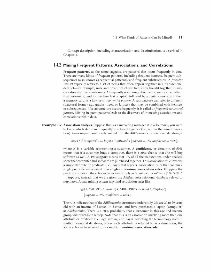
1.4 What Kinds of Patterns Can Be Mined? 17
Concept description, including characterization and discrimination, is described inChapter 4.
1.4.2 Mining Frequent Patterns, Associations, and Correlations
Frequent patterns, as the name suggests, are patterns that occur frequently in data.There are many kinds of frequent patterns, including frequent itemsets, frequent sub-sequences (also known as sequential patterns), and frequent substructures. A frequentitemset typically refers to a set of items that often appear together in a transactionaldata set—for example, milk and bread, which are frequently bought together in gro-cery stores by many customers. A frequently occurring subsequence, such as the patternthat customers, tend to purchase first a laptop, followed by a digital camera, and thena memory card, is a (frequent) sequential pattern. A substructure can refer to differentstructural forms (e.g., graphs, trees, or lattices) that may be combined with itemsetsor subsequences. If a substructure occurs frequently, it is called a (frequent) structuredpattern. Mining frequent patterns leads to the discovery of interesting associations andcorrelations within data.
Example 1.7 Association analysis. Suppose that, as a marketing manager at AllElectronics, you wantto know which items are frequently purchased together (i.e., within the same transac-tion). An example of such a rule, mined from the AllElectronics transactional database, is
buys(X , “computer”) ⇒ buys(X , “software”) [support = 1%, confidence = 50%],
where X is a variable representing a customer. A confidence, or certainty, of 50%means that if a customer buys a computer, there is a 50% chance that she will buysoftware as well. A 1% support means that 1% of all the transactions under analysisshow that computer and software are purchased together. This association rule involvesa single attribute or predicate (i.e., buys) that repeats. Association rules that contain asingle predicate are referred to as single-dimensional association rules. Dropping thepredicate notation, the rule can be written simply as “computer ⇒ software [1%, 50%].”
Suppose, instead, that we are given the AllElectronics relational database related topurchases. A data mining system may find association rules like
age(X , “20..29”) ∧ income(X , “40K..49K”) ⇒ buys(X , “laptop”)
[support = 2%, confidence = 60%].
The rule indicates that of the AllElectronics customers under study, 2% are 20 to 29 yearsold with an income of $40,000 to $49,000 and have purchased a laptop (computer)at AllElectronics. There is a 60% probability that a customer in this age and incomegroup will purchase a laptop. Note that this is an association involving more than oneattribute or predicate (i.e., age, income, and buys). Adopting the terminology used inmultidimensional databases, where each attribute is referred to as a dimension, theabove rule can be referred to as a multidimensional association rule.

18 Chapter 1 Introduction
Typically, association rules are discarded as uninteresting if they do not satisfy both aminimum support threshold and a minimum confidence threshold. Additional anal-ysis can be performed to uncover interesting statistical correlations between associatedattribute–value pairs.
Frequent itemset mining is a fundamental form of frequent pattern mining. The min-ing of frequent patterns, associations, and correlations is discussed in Chapters 6 and 7,where particular emphasis is placed on efficient algorithms for frequent itemset min-ing. Sequential pattern mining and structured pattern mining are considered advancedtopics.
1.4.3 Classification and Regression for Predictive Analysis
Classification is the process of finding a model (or function) that describes and distin-guishes data classes or concepts. The model are derived based on the analysis of a set oftraining data (i.e., data objects for which the class labels are known). The model is usedto predict the class label of objects for which the the class label is unknown.
“How is the derived model presented?” The derived model may be represented in var-ious forms, such as classification rules (i.e., IF-THEN rules), decision trees, mathematicalformulae, or neural networks (Figure 1.9). A decision tree is a flowchart-like tree structure,where each node denotes a test on an attribute value, each branch represents an outcomeof the test, and tree leaves represent classes or class distributions. Decision trees can easily
(a)
age(X, “youth”) AND income(X, “high”)
age(X, “youth”) AND income(X, “low”)
age(X, “middle_aged”)
age(X, “senior”)
class(X, “A”)
class(X, “B”)
class(X, “C”)
class(X, “C”)
middle_aged, senior
(b) (c)
age?
age f1
f2
f3
f4
f5
f6
f7
f8
income?income
youth
high low
class A
class A
class C
class C
class B
class B
Figure 1.9 A classification model can be represented in various forms: (a) IF-THEN rules, (b) a decisiontree, or (c) a neural network.

1.4 What Kinds of Patterns Can Be Mined? 19
be converted to classification rules. A neural network, when used for classification, is typ-ically a collection of neuron-like processing units with weighted connections between theunits. There are many other methods for constructing classification models, such as naıveBayesian classification, support vector machines, and k-nearest-neighbor classification.
Whereas classification predicts categorical (discrete, unordered) labels, regressionmodels continuous-valued functions. That is, regression is used to predict missing orunavailable numerical data values rather than (discrete) class labels. The term predictionrefers to both numeric prediction and class label prediction. Regression analysis is astatistical methodology that is most often used for numeric prediction, although othermethods exist as well. Regression also encompasses the identification of distributiontrends based on the available data.
Classification and regression may need to be preceded by relevance analysis, whichattempts to identify attributes that are significantly relevant to the classification andregression process. Such attributes will be selected for the classification and regressionprocess. Other attributes, which are irrelevant, can then be excluded from consideration.
Example 1.8 Classification and regression. Suppose as a sales manager of AllElectronics you want toclassify a large set of items in the store, based on three kinds of responses to a sales cam-paign: good response, mild response and no response. You want to derive a model for eachof these three classes based on the descriptive features of the items, such as price, brand,place made, type, and category. The resulting classification should maximally distinguisheach class from the others, presenting an organized picture of the data set.
Suppose that the resulting classification is expressed as a decision tree. The decisiontree, for instance, may identify price as being the single factor that best distinguishes thethree classes. The tree may reveal that, in addition to price, other features that help tofurther distinguish objects of each class from one another include brand and place made.Such a decision tree may help you understand the impact of the given sales campaignand design a more effective campaign in the future.
Suppose instead, that rather than predicting categorical response labels for each storeitem, you would like to predict the amount of revenue that each item will generateduring an upcoming sale at AllElectronics, based on the previous sales data. This is anexample of regression analysis because the regression model constructed will predict acontinuous function (or ordered value.)
Chapters 8 and 9 discuss classification in further detail. Regression analysis is beyondthe scope of this book. Sources for further information are given in the bibliographicnotes.
1.4.4 Cluster Analysis
Unlike classification and regression, which analyze class-labeled (training) data sets,clustering analyzes data objects without consulting class labels. In many cases, class-labeled data may simply not exist at the beginning. Clustering can be used to generate

20 Chapter 1 Introduction
Figure 1.10 A 2-D plot of customer data with respect to customer locations in a city, showing three dataclusters.
class labels for a group of data. The objects are clustered or grouped based on the princi-ple of maximizing the intraclass similarity and minimizing the interclass similarity. That is,clusters of objects are formed so that objects within a cluster have high similarity in com-parison to one another, but are rather dissimilar to objects in other clusters. Each clusterso formed can be viewed as a class of objects, from which rules can be derived. Clus-tering can also facilitate taxonomy formation, that is, the organization of observationsinto a hierarchy of classes that group similar events together.
Example 1.9 Cluster analysis. Cluster analysis can be performed on AllElectronics customer data toidentify homogeneous subpopulations of customers. These clusters may represent indi-vidual target groups for marketing. Figure 1.10 shows a 2-D plot of customers withrespect to customer locations in a city. Three clusters of data points are evident.
Cluster analysis forms the topic of Chapters 10 and 11.
1.4.5 Outlier Analysis
A data set may contain objects that do not comply with the general behavior or modelof the data. These data objects are outliers. Many data mining methods discard outliersas noise or exceptions. However, in some applications (e.g., fraud detection) the rare

1.4 What Kinds of Patterns Can Be Mined? 21
events can be more interesting than the more regularly occurring ones. The analysis ofoutlier data is referred to as outlier analysis or anomaly mining.
Outliers may be detected using statistical tests that assume a distribution or proba-bility model for the data, or using distance measures where objects that are remote fromany other cluster are considered outliers. Rather than using statistical or distance mea-sures, density-based methods may identify outliers in a local region, although they looknormal from a global statistical distribution view.
Example 1.10 Outlier analysis. Outlier analysis may uncover fraudulent usage of credit cards bydetecting purchases of unusually large amounts for a given account number in compari-son to regular charges incurred by the same account. Outlier values may also be detectedwith respect to the locations and types of purchase, or the purchase frequency.
Outlier analysis is discussed in Chapter 12.
1.4.6 Are All Patterns Interesting?
A data mining system has the potential to generate thousands or even millions ofpatterns, or rules.
You may ask, “Are all of the patterns interesting?” Typically, the answer is no—onlya small fraction of the patterns potentially generated would actually be of interest to agiven user.
This raises some serious questions for data mining. You may wonder, “What makes apattern interesting? Can a data mining system generate all of the interesting patterns? Or,Can the system generate only the interesting ones?”
To answer the first question, a pattern is interesting if it is (1) easily understood byhumans, (2) valid on new or test data with some degree of certainty, (3) potentiallyuseful, and (4) novel. A pattern is also interesting if it validates a hypothesis that the usersought to confirm. An interesting pattern represents knowledge.
Several objective measures of pattern interestingness exist. These are based onthe structure of discovered patterns and the statistics underlying them. An objectivemeasure for association rules of the form X ⇒ Y is rule support, representing the per-centage of transactions from a transaction database that the given rule satisfies. This istaken to be the probability P(X ∪ Y ), where X ∪ Y indicates that a transaction containsboth X and Y , that is, the union of itemsets X and Y . Another objective measure forassociation rules is confidence, which assesses the degree of certainty of the detectedassociation. This is taken to be the conditional probability P(Y |X), that is, the prob-ability that a transaction containing X also contains Y . More formally, support andconfidence are defined as
support(X ⇒ Y ) = P(X ∪ Y ),
confidence(X ⇒ Y ) = P(Y |X).
In general, each interestingness measure is associated with a threshold, which may becontrolled by the user. For example, rules that do not satisfy a confidence threshold of,

22 Chapter 1 Introduction
say, 50% can be considered uninteresting. Rules below the threshold likely reflect noise,exceptions, or minority cases and are probably of less value.
Other objective interestingness measures include accuracy and coverage for classifica-tion (IF-THEN) rules. In general terms, accuracy tells us the percentage of data that arecorrectly classified by a rule. Coverage is similar to support, in that it tells us the per-centage of data to which a rule applies. Regarding understandability, we may use simpleobjective measures that assess the complexity or length in bits of the patterns mined.
Although objective measures help identify interesting patterns, they are often insuffi-cient unless combined with subjective measures that reflect a particular user’s needs andinterests. For example, patterns describing the characteristics of customers who shopfrequently at AllElectronics should be interesting to the marketing manager, but may beof little interest to other analysts studying the same database for patterns on employeeperformance. Furthermore, many patterns that are interesting by objective standardsmay represent common sense and, therefore, are actually uninteresting.
Subjective interestingness measures are based on user beliefs in the data. Thesemeasures find patterns interesting if the patterns are unexpected (contradicting a user’sbelief) or offer strategic information on which the user can act. In the latter case, suchpatterns are referred to as actionable. For example, patterns like “a large earthquakeoften follows a cluster of small quakes” may be highly actionable if users can act on theinformation to save lives. Patterns that are expected can be interesting if they confirm ahypothesis that the user wishes to validate or they resemble a user’s hunch.
The second question—“Can a data mining system generate all of the interesting pat-terns?”—refers to the completeness of a data mining algorithm. It is often unrealisticand inefficient for data mining systems to generate all possible patterns. Instead, user-provided constraints and interestingness measures should be used to focus the search.For some mining tasks, such as association, this is often sufficient to ensure the com-pleteness of the algorithm. Association rule mining is an example where the use ofconstraints and interestingness measures can ensure the completeness of mining. Themethods involved are examined in detail in Chapter 6.
Finally, the third question—“Can a data mining system generate only interesting pat-terns?”—is an optimization problem in data mining. It is highly desirable for datamining systems to generate only interesting patterns. This would be efficient for usersand data mining systems because neither would have to search through the patterns gen-erated to identify the truly interesting ones. Progress has been made in this direction;however, such optimization remains a challenging issue in data mining.
Measures of pattern interestingness are essential for the efficient discovery of patternsby target users. Such measures can be used after the data mining step to rank the dis-covered patterns according to their interestingness, filtering out the uninteresting ones.More important, such measures can be used to guide and constrain the discovery pro-cess, improving the search efficiency by pruning away subsets of the pattern space thatdo not satisfy prespecified interestingness constraints. Examples of such a constraint-based mining process are described in Chapter 7 (with respect to pattern discovery) andChapter 11 (with respect to clustering).

1.5 Which Technologies Are Used? 23
Methods to assess pattern interestingness, and their use to improve data mining effi-ciency, are discussed throughout the book with respect to each kind of pattern that canbe mined.
1.5 Which Technologies Are Used?
As a highly application-driven domain, data mining has incorporated many techniquesfrom other domains such as statistics, machine learning, pattern recognition, databaseand data warehouse systems, information retrieval, visualization, algorithms, high-performance computing, and many application domains (Figure 1.11). The interdisci-plinary nature of data mining research and development contributes significantly to thesuccess of data mining and its extensive applications. In this section, we give examplesof several disciplines that strongly influence the development of data mining methods.
1.5.1 Statistics
Statistics studies the collection, analysis, interpretation or explanation, and presentationof data. Data mining has an inherent connection with statistics.
A statistical model is a set of mathematical functions that describe the behavior ofthe objects in a target class in terms of random variables and their associated proba-bility distributions. Statistical models are widely used to model data and data classes.For example, in data mining tasks like data characterization and classification, statistical
Statistics Machine learning Pattern recognition
Visualization
Algorithms
High-performancecomputing
ApplicationsInformationretrieval
Data warehouse
Database systems
Data Mining
Figure 1.11 Data mining adopts techniques from many domains.

24 Chapter 1 Introduction
models of target classes can be built. In other words, such statistical models can be theoutcome of a data mining task. Alternatively, data mining tasks can be built on top ofstatistical models. For example, we can use statistics to model noise and missing datavalues. Then, when mining patterns in a large data set, the data mining process can usethe model to help identify and handle noisy or missing values in the data.
Statistics research develops tools for prediction and forecasting using data and sta-tistical models. Statistical methods can be used to summarize or describe a collectionof data. Basic statistical descriptions of data are introduced in Chapter 2. Statistics isuseful for mining various patterns from data as well as for understanding the underlyingmechanisms generating and affecting the patterns. Inferential statistics (or predictivestatistics) models data in a way that accounts for randomness and uncertainty in theobservations and is used to draw inferences about the process or population underinvestigation.
Statistical methods can also be used to verify data mining results. For example, aftera classification or prediction model is mined, the model should be verified by statisti-cal hypothesis testing. A statistical hypothesis test (sometimes called confirmatory dataanalysis) makes statistical decisions using experimental data. A result is called statisticallysignificant if it is unlikely to have occurred by chance. If the classification or predictionmodel holds true, then the descriptive statistics of the model increases the soundness ofthe model.
Applying statistical methods in data mining is far from trivial. Often, a serious chal-lenge is how to scale up a statistical method over a large data set. Many statisticalmethods have high complexity in computation. When such methods are applied onlarge data sets that are also distributed on multiple logical or physical sites, algorithmsshould be carefully designed and tuned to reduce the computational cost. This challengebecomes even tougher for online applications, such as online query suggestions insearch engines, where data mining is required to continuously handle fast, real-timedata streams.
1.5.2 Machine Learning
Machine learning investigates how computers can learn (or improve their performance)based on data. A main research area is for computer programs to automatically learn torecognize complex patterns and make intelligent decisions based on data. For example, atypical machine learning problem is to program a computer so that it can automaticallyrecognize handwritten postal codes on mail after learning from a set of examples.
Machine learning is a fast-growing discipline. Here, we illustrate classic problems inmachine learning that are highly related to data mining.
Supervised learning is basically a synonym for classification. The supervision in thelearning comes from the labeled examples in the training data set. For example, inthe postal code recognition problem, a set of handwritten postal code images andtheir corresponding machine-readable translations are used as the training examples,which supervise the learning of the classification model.

1.5 Which Technologies Are Used? 25
Unsupervised learning is essentially a synonym for clustering. The learning processis unsupervised since the input examples are not class labeled. Typically, we may useclustering to discover classes within the data. For example, an unsupervised learningmethod can take, as input, a set of images of handwritten digits. Suppose that it finds10 clusters of data. These clusters may correspond to the 10 distinct digits of 0 to9, respectively. However, since the training data are not labeled, the learned modelcannot tell us the semantic meaning of the clusters found.
Semi-supervised learning is a class of machine learning techniques that make useof both labeled and unlabeled examples when learning a model. In one approach,labeled examples are used to learn class models and unlabeled examples are used torefine the boundaries between classes. For a two-class problem, we can think of theset of examples belonging to one class as the positive examples and those belongingto the other class as the negative examples. In Figure 1.12, if we do not consider theunlabeled examples, the dashed line is the decision boundary that best partitionsthe positive examples from the negative examples. Using the unlabeled examples,we can refine the decision boundary to the solid line. Moreover, we can detect thatthe two positive examples at the top right corner, though labeled, are likely noise oroutliers.
Active learning is a machine learning approach that lets users play an active rolein the learning process. An active learning approach can ask a user (e.g., a domainexpert) to label an example, which may be from a set of unlabeled examples orsynthesized by the learning program. The goal is to optimize the model quality byactively acquiring knowledge from human users, given a constraint on how manyexamples they can be asked to label.
Positive example
Negative example
Unlabeled example
Decision boundary without unlabeled examples
Decision boundary with unlabeled examples
Noise/outliers
Figure 1.12 Semi-supervised learning.

26 Chapter 1 Introduction
You can see there are many similarities between data mining and machine learning.For classification and clustering tasks, machine learning research often focuses on theaccuracy of the model. In addition to accuracy, data mining research places strongemphasis on the efficiency and scalability of mining methods on large data sets, as wellas on ways to handle complex types of data and explore new, alternative methods.
1.5.3 Database Systems and Data Warehouses
Database systems research focuses on the creation, maintenance, and use of databasesfor organizations and end-users. Particularly, database systems researchers have estab-lished highly recognized principles in data models, query languages, query processingand optimization methods, data storage, and indexing and accessing methods. Databasesystems are often well known for their high scalability in processing very large, relativelystructured data sets.
Many data mining tasks need to handle large data sets or even real-time, fast stream-ing data. Therefore, data mining can make good use of scalable database technologies toachieve high efficiency and scalability on large data sets. Moreover, data mining tasks canbe used to extend the capability of existing database systems to satisfy advanced users’sophisticated data analysis requirements.
Recent database systems have built systematic data analysis capabilities on databasedata using data warehousing and data mining facilities. A data warehouse integratesdata originating from multiple sources and various timeframes. It consolidates datain multidimensional space to form partially materialized data cubes. The data cubemodel not only facilitates OLAP in multidimensional databases but also promotesmultidimensional data mining (see Section 1.3.2).
1.5.4 Information Retrieval
Information retrieval (IR) is the science of searching for documents or informationin documents. Documents can be text or multimedia, and may reside on the Web. Thedifferences between traditional information retrieval and database systems are twofold:Information retrieval assumes that (1) the data under search are unstructured; and (2)the queries are formed mainly by keywords, which do not have complex structures(unlike SQL queries in database systems).
The typical approaches in information retrieval adopt probabilistic models. Forexample, a text document can be regarded as a bag of words, that is, a multiset of wordsappearing in the document. The document’s language model is the probability densityfunction that generates the bag of words in the document. The similarity between twodocuments can be measured by the similarity between their corresponding languagemodels.
Furthermore, a topic in a set of text documents can be modeled as a probability dis-tribution over the vocabulary, which is called a topic model. A text document, whichmay involve one or multiple topics, can be regarded as a mixture of multiple topic mod-els. By integrating information retrieval models and data mining techniques, we can find

1.6 Which Kinds of Applications Are Targeted? 27
the major topics in a collection of documents and, for each document in the collection,the major topics involved.
Increasingly large amounts of text and multimedia data have been accumulated andmade available online due to the fast growth of the Web and applications such as dig-ital libraries, digital governments, and health care information systems. Their effectivesearch and analysis have raised many challenging issues in data mining. Therefore, textmining and multimedia data mining, integrated with information retrieval methods,have become increasingly important.
1.6 Which Kinds of Applications Are Targeted?
Where there are data, there are data mining applications
As a highly application-driven discipline, data mining has seen great successes in manyapplications. It is impossible to enumerate all applications where data mining plays acritical role. Presentations of data mining in knowledge-intensive application domains,such as bioinformatics and software engineering, require more in-depth treatment andare beyond the scope of this book. To demonstrate the importance of applications asa major dimension in data mining research and development, we briefly discuss twohighly successful and popular application examples of data mining: business intelligenceand search engines.
1.6.1 Business Intelligence
It is critical for businesses to acquire a better understanding of the commercial contextof their organization, such as their customers, the market, supply and resources, andcompetitors. Business intelligence (BI) technologies provide historical, current, andpredictive views of business operations. Examples include reporting, online analyticalprocessing, business performance management, competitive intelligence, benchmark-ing, and predictive analytics.
“How important is business intelligence?” Without data mining, many businesses maynot be able to perform effective market analysis, compare customer feedback on simi-lar products, discover the strengths and weaknesses of their competitors, retain highlyvaluable customers, and make smart business decisions.
Clearly, data mining is the core of business intelligence. Online analytical process-ing tools in business intelligence rely on data warehousing and multidimensional datamining. Classification and prediction techniques are the core of predictive analyticsin business intelligence, for which there are many applications in analyzing markets,supplies, and sales. Moreover, clustering plays a central role in customer relationshipmanagement, which groups customers based on their similarities. Using characteriza-tion mining techniques, we can better understand features of each customer group anddevelop customized customer reward programs.

28 Chapter 1 Introduction
1.6.2 Web Search Engines
A Web search engine is a specialized computer server that searches for informationon the Web. The search results of a user query are often returned as a list (sometimescalled hits). The hits may consist of web pages, images, and other types of files. Somesearch engines also search and return data available in public databases or open directo-ries. Search engines differ from web directories in that web directories are maintainedby human editors whereas search engines operate algorithmically or by a mixture ofalgorithmic and human input.
Web search engines are essentially very large data mining applications. Various datamining techniques are used in all aspects of search engines, ranging from crawling5
(e.g., deciding which pages should be crawled and the crawling frequencies), indexing(e.g., selecting pages to be indexed and deciding to which extent the index should beconstructed), and searching (e.g., deciding how pages should be ranked, which adver-tisements should be added, and how the search results can be personalized or made“context aware”).
Search engines pose grand challenges to data mining. First, they have to handle ahuge and ever-growing amount of data. Typically, such data cannot be processed usingone or a few machines. Instead, search engines often need to use computer clouds, whichconsist of thousands or even hundreds of thousands of computers that collaborativelymine the huge amount of data. Scaling up data mining methods over computer cloudsand large distributed data sets is an area for further research.
Second, Web search engines often have to deal with online data. A search enginemay be able to afford constructing a model offline on huge data sets. To do this, it mayconstruct a query classifier that assigns a search query to predefined categories based onthe query topic (i.e., whether the search query “apple” is meant to retrieve informationabout a fruit or a brand of computers). Whether a model is constructed offline, theapplication of the model online must be fast enough to answer user queries in real time.
Another challenge is maintaining and incrementally updating a model on fast-growing data streams. For example, a query classifier may need to be incrementallymaintained continuously since new queries keep emerging and predefined categoriesand the data distribution may change. Most of the existing model training methods areoffline and static and thus cannot be used in such a scenario.
Third, Web search engines often have to deal with queries that are asked only a verysmall number of times. Suppose a search engine wants to provide context-aware queryrecommendations. That is, when a user poses a query, the search engine tries to inferthe context of the query using the user’s profile and his query history in order to returnmore customized answers within a small fraction of a second. However, although thetotal number of queries asked can be huge, most of the queries may be asked only onceor a few times. Such severely skewed data are challenging for many data mining andmachine learning methods.
5A Web crawler is a computer program that browses the Web in a methodical, automated manner.

1.7 Major Issues in Data Mining 29
1.7 Major Issues in Data Mining
Life is short but art is long. – Hippocrates
Data mining is a dynamic and fast-expanding field with great strengths. In this section,we briefly outline the major issues in data mining research, partitioning them intofive groups: mining methodology, user interaction, efficiency and scalability, diversity ofdata types, and data mining and society. Many of these issues have been addressed inrecent data mining research and development to a certain extent and are now consid-ered data mining requirements; others are still at the research stage. The issues continueto stimulate further investigation and improvement in data mining.
1.7.1 Mining Methodology
Researchers have been vigorously developing new data mining methodologies. Thisinvolves the investigation of new kinds of knowledge, mining in multidimensionalspace, integrating methods from other disciplines, and the consideration of semantic tiesamong data objects. In addition, mining methodologies should consider issues such asdata uncertainty, noise, and incompleteness. Some mining methods explore how user-specified measures can be used to assess the interestingness of discovered patterns aswell as guide the discovery process. Let’s have a look at these various aspects of miningmethodology.
Mining various and new kinds of knowledge: Data mining covers a wide spectrum ofdata analysis and knowledge discovery tasks, from data characterization and discrim-ination to association and correlation analysis, classification, regression, clustering,outlier analysis, sequence analysis, and trend and evolution analysis. These tasks mayuse the same database in different ways and require the development of numerousdata mining techniques. Due to the diversity of applications, new mining tasks con-tinue to emerge, making data mining a dynamic and fast-growing field. For example,for effective knowledge discovery in information networks, integrated clustering andranking may lead to the discovery of high-quality clusters and object ranks in largenetworks.
Mining knowledge in multidimensional space: When searching for knowledge in largedata sets, we can explore the data in multidimensional space. That is, we can searchfor interesting patterns among combinations of dimensions (attributes) at varyinglevels of abstraction. Such mining is known as (exploratory) multidimensional datamining. In many cases, data can be aggregated or viewed as a multidimensional datacube. Mining knowledge in cube space can substantially enhance the power andflexibility of data mining.
Data mining—an interdisciplinary effort: The power of data mining can be substan-tially enhanced by integrating new methods from multiple disciplines. For example,
30 Chapter 1 Introduction
to mine data with natural language text, it makes sense to fuse data mining methodswith methods of information retrieval and natural language processing. As anotherexample, consider the mining of software bugs in large programs. This form of min-ing, known as bug mining, benefits from the incorporation of software engineeringknowledge into the data mining process.
Boosting the power of discovery in a networked environment: Most data objects residein a linked or interconnected environment, whether it be the Web, database rela-tions, files, or documents. Semantic links across multiple data objects can be usedto advantage in data mining. Knowledge derived in one set of objects can be usedto boost the discovery of knowledge in a “related” or semantically linked set ofobjects.
Handling uncertainty, noise, or incompleteness of data: Data often contain noise,errors, exceptions, or uncertainty, or are incomplete. Errors and noise may confusethe data mining process, leading to the derivation of erroneous patterns. Data clean-ing, data preprocessing, outlier detection and removal, and uncertainty reasoning areexamples of techniques that need to be integrated with the data mining process.
Pattern evaluation and pattern- or constraint-guided mining: Not all the patterns gen-erated by data mining processes are interesting. What makes a pattern interestingmay vary from user to user. Therefore, techniques are needed to assess the inter-estingness of discovered patterns based on subjective measures. These estimate thevalue of patterns with respect to a given user class, based on user beliefs or expec-tations. Moreover, by using interestingness measures or user-specified constraints toguide the discovery process, we may generate more interesting patterns and reducethe search space.
1.7.2 User Interaction
The user plays an important role in the data mining process. Interesting areas of researchinclude how to interact with a data mining system, how to incorporate a user’s back-ground knowledge in mining, and how to visualize and comprehend data mining results.We introduce each of these here.
Interactive mining: The data mining process should be highly interactive. Thus, it isimportant to build flexible user interfaces and an exploratory mining environment,facilitating the user’s interaction with the system. A user may like to first sample aset of data, explore general characteristics of the data, and estimate potential min-ing results. Interactive mining should allow users to dynamically change the focusof a search, to refine mining requests based on returned results, and to drill, dice,and pivot through the data and knowledge space interactively, dynamically exploring“cube space” while mining.
Incorporation of background knowledge: Background knowledge, constraints, rules,and other information regarding the domain under study should be incorporated

1.7 Major Issues in Data Mining 31
into the knowledge discovery process. Such knowledge can be used for patternevaluation as well as to guide the search toward interesting patterns.
Ad hoc data mining and data mining query languages: Query languages (e.g., SQL)have played an important role in flexible searching because they allow users to posead hoc queries. Similarly, high-level data mining query languages or other high-levelflexible user interfaces will give users the freedom to define ad hoc data mining tasks.This should facilitate specification of the relevant sets of data for analysis, the domainknowledge, the kinds of knowledge to be mined, and the conditions and constraintsto be enforced on the discovered patterns. Optimization of the processing of suchflexible mining requests is another promising area of study.
Presentation and visualization of data mining results: How can a data mining systempresent data mining results, vividly and flexibly, so that the discovered knowledgecan be easily understood and directly usable by humans? This is especially crucialif the data mining process is interactive. It requires the system to adopt expressiveknowledge representations, user-friendly interfaces, and visualization techniques.
1.7.3 Efficiency and Scalability
Efficiency and scalability are always considered when comparing data mining algo-rithms. As data amounts continue to multiply, these two factors are especially critical.
Efficiency and scalability of data mining algorithms: Data mining algorithms must beefficient and scalable in order to effectively extract information from huge amountsof data in many data repositories or in dynamic data streams. In other words, therunning time of a data mining algorithm must be predictable, short, and acceptableby applications. Efficiency, scalability, performance, optimization, and the ability toexecute in real time are key criteria that drive the development of many new datamining algorithms.
Parallel, distributed, and incremental mining algorithms: The humongous size of manydata sets, the wide distribution of data, and the computational complexity of somedata mining methods are factors that motivate the development of parallel and dis-tributed data-intensive mining algorithms. Such algorithms first partition the datainto “pieces.” Each piece is processed, in parallel, by searching for patterns. The par-allel processes may interact with one another. The patterns from each partition areeventually merged.
Cloud computing and cluster computing, which use computers in a distributedand collaborative way to tackle very large-scale computational tasks, are also activeresearch themes in parallel data mining. In addition, the high cost of some data min-ing processes and the incremental nature of input promote incremental data mining,which incorporates new data updates without having to mine the entire data “fromscratch.” Such methods perform knowledge modification incrementally to amendand strengthen what was previously discovered.

32 Chapter 1 Introduction
1.7.4 Diversity of Database Types
The wide diversity of database types brings about challenges to data mining. Theseinclude
Handling complex types of data: Diverse applications generate a wide spectrum ofnew data types, from structured data such as relational and data warehouse data tosemi-structured and unstructured data; from stable data repositories to dynamic datastreams; from simple data objects to temporal data, biological sequences, sensor data,spatial data, hypertext data, multimedia data, software program code, Web data, andsocial network data. It is unrealistic to expect one data mining system to mine allkinds of data, given the diversity of data types and the different goals of data mining.Domain- or application-dedicated data mining systems are being constructed for in-depth mining of specific kinds of data. The construction of effective and efficientdata mining tools for diverse applications remains a challenging and active area ofresearch.
Mining dynamic, networked, and global data repositories: Multiple sources of dataare connected by the Internet and various kinds of networks, forming gigantic, dis-tributed, and heterogeneous global information systems and networks. The discoveryof knowledge from different sources of structured, semi-structured, or unstructuredyet interconnected data with diverse data semantics poses great challenges to datamining. Mining such gigantic, interconnected information networks may help dis-close many more patterns and knowledge in heterogeneous data sets than can be dis-covered from a small set of isolated data repositories. Web mining, multisource datamining, and information network mining have become challenging and fast-evolvingdata mining fields.
1.7.5 Data Mining and Society
How does data mining impact society? What steps can data mining take to preserve theprivacy of individuals? Do we use data mining in our daily lives without even knowingthat we do? These questions raise the following issues:
Social impacts of data mining: With data mining penetrating our everyday lives, it isimportant to study the impact of data mining on society. How can we use data miningtechnology to benefit society? How can we guard against its misuse? The improperdisclosure or use of data and the potential violation of individual privacy and dataprotection rights are areas of concern that need to be addressed.
Privacy-preserving data mining: Data mining will help scientific discovery, businessmanagement, economy recovery, and security protection (e.g., the real-time dis-covery of intruders and cyberattacks). However, it poses the risk of disclosing anindividual’s personal information. Studies on privacy-preserving data publishing anddata mining are ongoing. The philosophy is to observe data sensitivity and preservepeople’s privacy while performing successful data mining.

1.8 Summary 33
Invisible data mining: We cannot expect everyone in society to learn and masterdata mining techniques. More and more systems should have data mining func-tions built within so that people can perform data mining or use data mining resultssimply by mouse clicking, without any knowledge of data mining algorithms. Intelli-gent search engines and Internet-based stores perform such invisible data mining byincorporating data mining into their components to improve their functionality andperformance. This is done often unbeknownst to the user. For example, when pur-chasing items online, users may be unaware that the store is likely collecting data onthe buying patterns of its customers, which may be used to recommend other itemsfor purchase in the future.
These issues and many additional ones relating to the research, development, andapplication of data mining are discussed throughout the book.
1.8 Summary
Necessity is the mother of invention. With the mounting growth of data in every appli-cation, data mining meets the imminent need for effective, scalable, and flexible dataanalysis in our society. Data mining can be considered as a natural evolution of infor-mation technology and a confluence of several related disciplines and applicationdomains.
Data mining is the process of discovering interesting patterns from massive amountsof data. As a knowledge discovery process, it typically involves data cleaning, data inte-gration, data selection, data transformation, pattern discovery, pattern evaluation,and knowledge presentation.
A pattern is interesting if it is valid on test data with some degree of certainty, novel,potentially useful (e.g., can be acted on or validates a hunch about which the user wascurious), and easily understood by humans. Interesting patterns represent knowl-edge. Measures of pattern interestingness, either objective or subjective, can be usedto guide the discovery process.
We present a multidimensional view of data mining. The major dimensions aredata, knowledge, technologies, and applications.
Data mining can be conducted on any kind of data as long as the data are meaningfulfor a target application, such as database data, data warehouse data, transactionaldata, and advanced data types. Advanced data types include time-related or sequencedata, data streams, spatial and spatiotemporal data, text and multimedia data, graphand networked data, and Web data.
A data warehouse is a repository for long-term storage of data from multiple sources,organized so as to facilitate management decision making. The data are storedunder a unified schema and are typically summarized. Data warehouse systems pro-vide multidimensional data analysis capabilities, collectively referred to as onlineanalytical processing.

34 Chapter 1 Introduction
Multidimensional data mining (also called exploratory multidimensional datamining) integrates core data mining techniques with OLAP-based multidimen-sional analysis. It searches for interesting patterns among multiple combinationsof dimensions (attributes) at varying levels of abstraction, thereby exploring multi-dimensional data space.
Data mining functionalities are used to specify the kinds of patterns or knowledgeto be found in data mining tasks. The functionalities include characterization anddiscrimination; the mining of frequent patterns, associations, and correlations; clas-sification and regression; cluster analysis; and outlier detection. As new types of data,new applications, and new analysis demands continue to emerge, there is no doubtwe will see more and more novel data mining tasks in the future.
Data mining, as a highly application-driven domain, has incorporated technologiesfrom many other domains. These include statistics, machine learning, database anddata warehouse systems, and information retrieval. The interdisciplinary nature ofdata mining research and development contributes significantly to the success ofdata mining and its extensive applications.
Data mining has many successful applications, such as business intelligence, Websearch, bioinformatics, health informatics, finance, digital libraries, and digitalgovernments.
There are many challenging issues in data mining research. Areas include miningmethodology, user interaction, efficiency and scalability, and dealing with diversedata types. Data mining research has strongly impacted society and will continue todo so in the future.
1.9 Exercises
1.1 What is data mining? In your answer, address the following:
(a) Is it another hype?
(b) Is it a simple transformation or application of technology developed from databases,statistics, machine learning, and pattern recognition?
(c) We have presented a view that data mining is the result of the evolution of databasetechnology. Do you think that data mining is also the result of the evolution ofmachine learning research? Can you present such views based on the historicalprogress of this discipline? Address the same for the fields of statistics and patternrecognition.
(d) Describe the steps involved in data mining when viewed as a process of knowledgediscovery.
1.2 How is a data warehouse different from a database? How are they similar?
1.3 Define each of the following data mining functionalities: characterization, discrimi-nation, association and correlation analysis, classification, regression, clustering, and

1.10 Bibliographic Notes 35
outlier analysis. Give examples of each data mining functionality, using a real-lifedatabase that you are familiar with.
1.4 Present an example where data mining is crucial to the success of a business. What datamining functionalities does this business need (e.g., think of the kinds of patterns thatcould be mined)? Can such patterns be generated alternatively by data query processingor simple statistical analysis?
1.5 Explain the difference and similarity between discrimination and classification, betweencharacterization and clustering, and between classification and regression.
1.6 Based on your observations, describe another possible kind of knowledge that needs tobe discovered by data mining methods but has not been listed in this chapter. Does itrequire a mining methodology that is quite different from those outlined in this chapter?
1.7 Outliers are often discarded as noise. However, one person’s garbage could be another’streasure. For example, exceptions in credit card transactions can help us detect thefraudulent use of credit cards. Using fraudulence detection as an example, propose twomethods that can be used to detect outliers and discuss which one is more reliable.
1.8 Describe three challenges to data mining regarding data mining methodology and userinteraction issues.
1.9 What are the major challenges of mining a huge amount of data (e.g., billions of tuples)in comparison with mining a small amount of data (e.g., data set of a few hundredtuple)?
1.10 Outline the major research challenges of data mining in one specific application domain,such as stream/sensor data analysis, spatiotemporal data analysis, or bioinformatics.
1.10 Bibliographic Notes
The book Knowledge Discovery in Databases, edited by Piatetsky-Shapiro and Frawley[P-SF91], is an early collection of research papers on knowledge discovery from data.The book Advances in Knowledge Discovery and Data Mining, edited by Fayyad,Piatetsky-Shapiro, Smyth, and Uthurusamy [FPSS+96], is a collection of later researchresults on knowledge discovery and data mining. There have been many data min-ing books published in recent years, including The Elements of Statistical Learningby Hastie, Tibshirani, and Friedman [HTF09]; Introduction to Data Mining by Tan,Steinbach, and Kumar [TSK05]; Data Mining: Practical Machine Learning Tools andTechniques with Java Implementations by Witten, Frank, and Hall [WFH11]; Predic-tive Data Mining by Weiss and Indurkhya [WI98]; Mastering Data Mining: The Artand Science of Customer Relationship Management by Berry and Linoff [BL99]; Prin-ciples of Data Mining (Adaptive Computation and Machine Learning) by Hand, Mannila,and Smyth [HMS01]; Mining the Web: Discovering Knowledge from Hypertext Data byChakrabarti [Cha03a]; Web Data Mining: Exploring Hyperlinks, Contents, and Usage

36 Chapter 1 Introduction
Data by Liu [Liu06]; Data Mining: Introductory and Advanced Topics by Dunham[Dun03]; and Data Mining: Multimedia, Soft Computing, and Bioinformatics by Mitraand Acharya [MA03].
There are also books that contain collections of papers or chapters on particularaspects of knowledge discovery—for example, Relational Data Mining edited by Dze-roski and Lavrac [De01]; Mining Graph Data edited by Cook and Holder [CH07]; DataStreams: Models and Algorithms edited by Aggarwal [Agg06]; Next Generation of DataMining edited by Kargupta, Han, Yu, et al. [KHY+08]; Multimedia Data Mining: A Sys-tematic Introduction to Concepts and Theory edited by Z. Zhang and R. Zhang [ZZ09];Geographic Data Mining and Knowledge Discovery edited by Miller and Han [MH09];and Link Mining: Models, Algorithms and Applications edited by Yu, Han, and Falout-sos [YHF10]. There are many tutorial notes on data mining in major databases, datamining, machine learning, statistics, and Web technology conferences.
KDNuggets is a regular electronic newsletter containing information relevant toknowledge discovery and data mining, moderated by Piatetsky-Shapiro since 1991.The Internet site KDNuggets (www.kdnuggets.com) contains a good collection of KDD-related information.
The data mining community started its first international conference on knowledgediscovery and data mining in 1995. The conference evolved from the four inter-national workshops on knowledge discovery in databases, held from 1989 to 1994.ACM-SIGKDD, a Special Interest Group on Knowledge Discovery in Databases wasset up under ACM in 1998 and has been organizing the international conferences onknowledge discovery and data mining since 1999. IEEE Computer Science Society hasorganized its annual data mining conference, International Conference on Data Min-ing (ICDM), since 2001. SIAM (Society on Industrial and Applied Mathematics) hasorganized its annual data mining conference, SIAM Data Mining Conference (SDM),since 2002. A dedicated journal, Data Mining and Knowledge Discovery, published byKluwers Publishers, has been available since 1997. An ACM journal, ACM Transactionson Knowledge Discovery from Data, published its first volume in 2007.
ACM-SIGKDD also publishes a bi-annual newsletter, SIGKDD Explorations. Thereare a few other international or regional conferences on data mining, such as theEuropean Conference on Machine Learning and Principles and Practice of KnowledgeDiscovery in Databases (ECML PKDD), the Pacific-Asia Conference on KnowledgeDiscovery and Data Mining (PAKDD), and the International Conference on DataWarehousing and Knowledge Discovery (DaWaK).
Research in data mining has also been published in books, conferences, and jour-nals on databases, statistics, machine learning, and data visualization. References to suchsources are listed at the end of the book.
Popular textbooks on database systems include Database Systems: The Complete Bookby Garcia-Molina, Ullman, and Widom [GMUW08]; Database Management Systems byRamakrishnan and Gehrke [RG03]; Database System Concepts by Silberschatz, Korth,and Sudarshan [SKS10]; and Fundamentals of Database Systems by Elmasri and Navathe[EN10]. For an edited collection of seminal articles on database systems, see Readings inDatabase Systems by Hellerstein and Stonebraker [HS05].

1.10 Bibliographic Notes 37
There are also many books on data warehouse technology, systems, and applica-tions, such as The Data Warehouse Toolkit: The Complete Guide to Dimensional Modelingby Kimball and Ross [KR02]; The Data Warehouse Lifecycle Toolkit by Kimball, Ross,Thornthwaite, and Mundy [KRTM08]; Mastering Data Warehouse Design: Relationaland Dimensional Techniques by Imhoff, Galemmo, and Geiger [IGG03]; and Buildingthe Data Warehouse by Inmon [Inm96]. A set of research papers on materialized viewsand data warehouse implementations were collected in Materialized Views: Techniques,Implementations, and Applications by Gupta and Mumick [GM99]. Chaudhuri andDayal [CD97] present an early comprehensive overview of data warehouse technology.
Research results relating to data mining and data warehousing have been pub-lished in the proceedings of many international database conferences, including theACM-SIGMOD International Conference on Management of Data (SIGMOD), theInternational Conference on Very Large Data Bases (VLDB), the ACM SIGACT-SIGMOD-SIGART Symposium on Principles of Database Systems (PODS), the Inter-national Conference on Data Engineering (ICDE), the International Conference onExtending Database Technology (EDBT), the International Conference on DatabaseTheory (ICDT), the International Conference on Information and Knowledge Man-agement (CIKM), the International Conference on Database and Expert Systems Appli-cations (DEXA), and the International Symposium on Database Systems for AdvancedApplications (DASFAA). Research in data mining is also published in major databasejournals, such as IEEE Transactions on Knowledge and Data Engineering (TKDE), ACMTransactions on Database Systems (TODS), Information Systems, The VLDB Journal,Data and Knowledge Engineering, International Journal of Intelligent Information Systems(JIIS), and Knowledge and Information Systems (KAIS).
Many effective data mining methods have been developed by statisticians and intro-duced in a rich set of textbooks. An overview of classification from a statistical patternrecognition perspective can be found in Pattern Classification by Duda, Hart, and Stork[DHS01]. There are also many textbooks covering regression and other topics in statis-tical analysis, such as Mathematical Statistics: Basic Ideas and Selected Topics by Bickeland Doksum [BD01]; The Statistical Sleuth: A Course in Methods of Data Analysis byRamsey and Schafer [RS01]; Applied Linear Statistical Models by Neter, Kutner, Nacht-sheim, and Wasserman [NKNW96]; An Introduction to Generalized Linear Models byDobson [Dob90]; Applied Statistical Time Series Analysis by Shumway [Shu88]; andApplied Multivariate Statistical Analysis by Johnson and Wichern [JW92].
Research in statistics is published in the proceedings of several major statistical con-ferences, including Joint Statistical Meetings, International Conference of the RoyalStatistical Society and Symposium on the Interface: Computing Science and Statistics.Other sources of publication include the Journal of the Royal Statistical Society, TheAnnals of Statistics, the Journal of American Statistical Association, Technometrics, andBiometrika.
Textbooks and reference books on machine learning and pattern recognition includeMachine Learning by Mitchell [Mit97]; Pattern Recognition and Machine Learning byBishop [Bis06]; Pattern Recognition by Theodoridis and Koutroumbas [TK08]; Introduc-tion to Machine Learning by Alpaydin [Alp11]; Probabilistic Graphical Models: Principles

38 Chapter 1 Introduction
and Techniques by Koller and Friedman [KF09]; and Machine Learning: An AlgorithmicPerspective by Marsland [Mar09]. For an edited collection of seminal articles on machinelearning, see Machine Learning, An Artificial Intelligence Approach, Volumes 1 through 4,edited by Michalski et al. [MCM83, MCM86, KM90, MT94], and Readings in MachineLearning by Shavlik and Dietterich [SD90].
Machine learning and pattern recognition research is published in the proceed-ings of several major machine learning, artificial intelligence, and pattern recognitionconferences, including the International Conference on Machine Learning (ML), theACM Conference on Computational Learning Theory (COLT), the IEEE Conferenceon Computer Vision and Pattern Recognition (CVPR), the International Conferenceon Pattern Recognition (ICPR), the International Joint Conference on Artificial Intel-ligence (IJCAI), and the American Association of Artificial Intelligence Conference(AAAI). Other sources of publication include major machine learning, artificial intel-ligence, pattern recognition, and knowledge system journals, some of which have beenmentioned before. Others include Machine Learning (ML), Pattern Recognition (PR),Artificial Intelligence Journal (AI), IEEE Transactions on Pattern Analysis and MachineIntelligence (PAMI), and Cognitive Science.
Textbooks and reference books on information retrieval include Introduction toInformation Retrieval by Manning, Raghavan, and Schutz [MRS08]; InformationRetrieval: Implementing and Evaluating Search Engines by Buttcher, Clarke, and Cormack[BCC10]; Search Engines: Information Retrieval in Practice by Croft, Metzler, andStrohman [CMS09]; Modern Information Retrieval: The Concepts and Technology BehindSearch by Baeza-Yates and Ribeiro-Neto [BYRN11]; and Information Retrieval: Algo-rithms and Heuristics by Grossman and Frieder [GR04].
Information retrieval research is published in the proceedings of several informa-tion retrieval and Web search and mining conferences, including the InternationalACM SIGIR Conference on Research and Development in Information Retrieval(SIGIR), the International World Wide Web Conference (WWW), the ACM Interna-tional Conference on Web Search and Data Mining (WSDM), the ACM Conference onInformation and Knowledge Management (CIKM), the European Conference on Infor-mation Retrieval (ECIR), the Text Retrieval Conference (TREC), and the ACM/IEEEJoint Conference on Digital Libraries (JCDL). Other sources of publication includemajor information retrieval, information systems, and Web journals, such as Journalof Information Retrieval, ACM Transactions on Information Systems (TOIS), Informa-tion Processing and Management, Knowledge and Information Systems (KAIS), and IEEETransactions on Knowledge and Data Engineering (TKDE).

2Getting to Know Your Data
It’s tempting to jump straight into mining, but first, we need to get the data ready. This involveshaving a closer look at attributes and data values. Real-world data are typically noisy,enormous in volume (often several gigabytes or more), and may originate from a hodge-podge of heterogenous sources. This chapter is about getting familiar with your data.Knowledge about your data is useful for data preprocessing (see Chapter 3), the firstmajor task of the data mining process. You will want to know the following: What arethe types of attributes or fields that make up your data? What kind of values does eachattribute have? Which attributes are discrete, and which are continuous-valued? Whatdo the data look like? How are the values distributed? Are there ways we can visualizethe data to get a better sense of it all? Can we spot any outliers? Can we measure thesimilarity of some data objects with respect to others? Gaining such insight into the datawill help with the subsequent analysis.
“So what can we learn about our data that’s helpful in data preprocessing?” We beginin Section 2.1 by studying the various attribute types. These include nominal attributes,binary attributes, ordinal attributes, and numeric attributes. Basic statistical descriptionscan be used to learn more about each attribute’s values, as described in Section 2.2.Given a temperature attribute, for example, we can determine its mean (average value),median (middle value), and mode (most common value). These are measures ofcentral tendency, which give us an idea of the “middle” or center of distribution.
Knowing such basic statistics regarding each attribute makes it easier to fill in missingvalues, smooth noisy values, and spot outliers during data preprocessing. Knowledge ofthe attributes and attribute values can also help in fixing inconsistencies incurred dur-ing data integration. Plotting the measures of central tendency shows us if the data aresymmetric or skewed. Quantile plots, histograms, and scatter plots are other graphic dis-plays of basic statistical descriptions. These can all be useful during data preprocessingand can provide insight into areas for mining.
The field of data visualization provides many additional techniques for viewing datathrough graphical means. These can help identify relations, trends, and biases “hidden”in unstructured data sets. Techniques may be as simple as scatter-plot matrices (where
c© 2012 Elsevier Inc. All rights reserved.
Data Mining: Concepts and Techniques 39

40 Chapter 2 Getting to Know Your Data
two attributes are mapped onto a 2-D grid) to more sophisticated methods such as tree-maps (where a hierarchical partitioning of the screen is displayed based on the attributevalues). Data visualization techniques are described in Section 2.3.
Finally, we may want to examine how similar (or dissimilar) data objects are. Forexample, suppose we have a database where the data objects are patients, described bytheir symptoms. We may want to find the similarity or dissimilarity between individ-ual patients. Such information can allow us to find clusters of like patients within thedata set. The similarity/dissimilarity between objects may also be used to detect out-liers in the data, or to perform nearest-neighbor classification. (Clustering is the topicof Chapters 10 and 11, while nearest-neighbor classification is discussed in Chapter 9.)There are many measures for assessing similarity and dissimilarity. In general, such mea-sures are referred to as proximity measures. Think of the proximity of two objects as afunction of the distance between their attribute values, although proximity can also becalculated based on probabilities rather than actual distance. Measures of data proximityare described in Section 2.4.
In summary, by the end of this chapter, you will know the different attribute typesand basic statistical measures to describe the central tendency and dispersion (spread)of attribute data. You will also know techniques to visualize attribute distributions andhow to compute the similarity or dissimilarity between objects.
2.1 Data Objects and Attribute Types
Data sets are made up of data objects. A data object represents an entity—in a salesdatabase, the objects may be customers, store items, and sales; in a medical database, theobjects may be patients; in a university database, the objects may be students, professors,and courses. Data objects are typically described by attributes. Data objects can also bereferred to as samples, examples, instances, data points, or objects. If the data objects arestored in a database, they are data tuples. That is, the rows of a database correspond tothe data objects, and the columns correspond to the attributes. In this section, we defineattributes and look at the various attribute types.
2.1.1 What Is an Attribute?
An attribute is a data field, representing a characteristic or feature of a data object. Thenouns attribute, dimension, feature, and variable are often used interchangeably in theliterature. The term dimension is commonly used in data warehousing. Machine learningliterature tends to use the term feature, while statisticians prefer the term variable. Datamining and database professionals commonly use the term attribute, and we do hereas well. Attributes describing a customer object can include, for example, customer ID,name, and address. Observed values for a given attribute are known as observations. A setof attributes used to describe a given object is called an attribute vector (or feature vec-tor). The distribution of data involving one attribute (or variable) is called univariate.A bivariate distribution involves two attributes, and so on.

2.1 Data Objects and Attribute Types 41
The type of an attribute is determined by the set of possible values—nominal, binary,ordinal, or numeric—the attribute can have. In the following subsections, we introduceeach type.
2.1.2 Nominal Attributes
Nominal means “relating to names.” The values of a nominal attribute are symbols ornames of things. Each value represents some kind of category, code, or state, and so nomi-nal attributes are also referred to as categorical. The values do not have any meaningfulorder. In computer science, the values are also known as enumerations.
Example 2.1 Nominal attributes. Suppose that hair color and marital status are two attributesdescribing person objects. In our application, possible values for hair color are black,brown, blond, red, auburn, gray, and white. The attribute marital status can take onthe values single, married, divorced, and widowed. Both hair color and marital statusare nominal attributes. Another example of a nominal attribute is occupation, with thevalues teacher, dentist, programmer, farmer, and so on.
Although we said that the values of a nominal attribute are symbols or “namesof things,” it is possible to represent such symbols or “names” with numbers. Withhair color, for instance, we can assign a code of 0 for black, 1 for brown, and so on.Another example is customor ID, with possible values that are all numeric. However,in such cases, the numbers are not intended to be used quantitatively. That is, mathe-matical operations on values of nominal attributes are not meaningful. It makes nosense to subtract one customer ID number from another, unlike, say, subtracting an agevalue from another (where age is a numeric attribute). Even though a nominal attributemay have integers as values, it is not considered a numeric attribute because the inte-gers are not meant to be used quantitatively. We will say more on numeric attributes inSection 2.1.5.
Because nominal attribute values do not have any meaningful order about them andare not quantitative, it makes no sense to find the mean (average) value or median(middle) value for such an attribute, given a set of objects. One thing that is of inter-est, however, is the attribute’s most commonly occurring value. This value, known asthe mode, is one of the measures of central tendency. You will learn about measures ofcentral tendency in Section 2.2.
2.1.3 Binary Attributes
A binary attribute is a nominal attribute with only two categories or states: 0 or 1, where0 typically means that the attribute is absent, and 1 means that it is present. Binaryattributes are referred to as Boolean if the two states correspond to true and false.
Example 2.2 Binary attributes. Given the attribute smoker describing a patient object, 1 indicatesthat the patient smokes, while 0 indicates that the patient does not. Similarly, suppose

42 Chapter 2 Getting to Know Your Data
the patient undergoes a medical test that has two possible outcomes. The attributemedical test is binary, where a value of 1 means the result of the test for the patientis positive, while 0 means the result is negative.
A binary attribute is symmetric if both of its states are equally valuable and carrythe same weight; that is, there is no preference on which outcome should be codedas 0 or 1. One such example could be the attribute gender having the states male andfemale.
A binary attribute is asymmetric if the outcomes of the states are not equally impor-tant, such as the positive and negative outcomes of a medical test for HIV. By convention,we code the most important outcome, which is usually the rarest one, by 1 (e.g., HIVpositive) and the other by 0 (e.g., HIV negative).
2.1.4 Ordinal Attributes
An ordinal attribute is an attribute with possible values that have a meaningful order orranking among them, but the magnitude between successive values is not known.
Example 2.3 Ordinal attributes. Suppose that drink size corresponds to the size of drinks available ata fast-food restaurant. This nominal attribute has three possible values: small, medium,and large. The values have a meaningful sequence (which corresponds to increasingdrink size); however, we cannot tell from the values how much bigger, say, a mediumis than a large. Other examples of ordinal attributes include grade (e.g., A+, A, A−, B+,and so on) and professional rank. Professional ranks can be enumerated in a sequentialorder: for example, assistant, associate, and full for professors, and private, private firstclass, specialist, corporal, and sergeant for army ranks.
Ordinal attributes are useful for registering subjective assessments of qualities thatcannot be measured objectively; thus ordinal attributes are often used in surveys forratings. In one survey, participants were asked to rate how satisfied they were as cus-tomers. Customer satisfaction had the following ordinal categories: 0: very dissatisfied,1: somewhat dissatisfied, 2: neutral, 3: satisfied, and 4: very satisfied.
Ordinal attributes may also be obtained from the discretization of numeric quantitiesby splitting the value range into a finite number of ordered categories as described inChapter 3 on data reduction.
The central tendency of an ordinal attribute can be represented by its mode and itsmedian (the middle value in an ordered sequence), but the mean cannot be defined.
Note that nominal, binary, and ordinal attributes are qualitative. That is, they describea feature of an object without giving an actual size or quantity. The values of suchqualitative attributes are typically words representing categories. If integers are used,they represent computer codes for the categories, as opposed to measurable quantities(e.g., 0 for small drink size, 1 for medium, and 2 for large). In the following subsec-tion we look at numeric attributes, which provide quantitative measurements of anobject.

2.1 Data Objects and Attribute Types 43
2.1.5 Numeric Attributes
A numeric attribute is quantitative; that is, it is a measurable quantity, represented ininteger or real values. Numeric attributes can be interval-scaled or ratio-scaled.
Interval-Scaled AttributesInterval-scaled attributes are measured on a scale of equal-size units. The values ofinterval-scaled attributes have order and can be positive, 0, or negative. Thus, in additionto providing a ranking of values, such attributes allow us to compare and quantify thedifference between values.
Example 2.4 Interval-scaled attributes. A temperature attribute is interval-scaled. Suppose that wehave the outdoor temperature value for a number of different days, where each day isan object. By ordering the values, we obtain a ranking of the objects with respect totemperature. In addition, we can quantify the difference between values. For example, atemperature of 20◦C is five degrees higher than a temperature of 15◦C. Calendar datesare another example. For instance, the years 2002 and 2010 are eight years apart.
Temperatures in Celsius and Fahrenheit do not have a true zero-point, that is, neither0◦C nor 0◦F indicates “no temperature.” (On the Celsius scale, for example, the unit ofmeasurement is 1/100 of the difference between the melting temperature and the boilingtemperature of water in atmospheric pressure.) Although we can compute the differencebetween temperature values, we cannot talk of one temperature value as being a multipleof another. Without a true zero, we cannot say, for instance, that 10◦C is twice as warmas 5◦C. That is, we cannot speak of the values in terms of ratios. Similarly, there is notrue zero-point for calendar dates. (The year 0 does not correspond to the beginning oftime.) This brings us to ratio-scaled attributes, for which a true zero-point exits.
Because interval-scaled attributes are numeric, we can compute their mean value, inaddition to the median and mode measures of central tendency.
Ratio-Scaled AttributesA ratio-scaled attribute is a numeric attribute with an inherent zero-point. That is, ifa measurement is ratio-scaled, we can speak of a value as being a multiple (or ratio)of another value. In addition, the values are ordered, and we can also compute thedifference between values, as well as the mean, median, and mode.
Example 2.5 Ratio-scaled attributes. Unlike temperatures in Celsius and Fahrenheit, the Kelvin (K)temperature scale has what is considered a true zero-point (0◦K = −273.15◦C): It isthe point at which the particles that comprise matter have zero kinetic energy. Otherexamples of ratio-scaled attributes include count attributes such as years of experience(e.g., the objects are employees) and number of words (e.g., the objects are documents).Additional examples include attributes to measure weight, height, latitude and longitude

44 Chapter 2 Getting to Know Your Data
coordinates (e.g., when clustering houses), and monetary quantities (e.g., you are 100times richer with $100 than with $1).
2.1.6 Discrete versus Continuous Attributes
In our presentation, we have organized attributes into nominal, binary, ordinal, andnumeric types. There are many ways to organize attribute types. The types are notmutually exclusive.
Classification algorithms developed from the field of machine learning often talk ofattributes as being either discrete or continuous. Each type may be processed differently.A discrete attribute has a finite or countably infinite set of values, which may or may notbe represented as integers. The attributes hair color, smoker, medical test, and drink sizeeach have a finite number of values, and so are discrete. Note that discrete attributesmay have numeric values, such as 0 and 1 for binary attributes or, the values 0 to 110 forthe attribute age. An attribute is countably infinite if the set of possible values is infinitebut the values can be put in a one-to-one correspondence with natural numbers. Forexample, the attribute customer ID is countably infinite. The number of customers cangrow to infinity, but in reality, the actual set of values is countable (where the values canbe put in one-to-one correspondence with the set of integers). Zip codes are anotherexample.
If an attribute is not discrete, it is continuous. The terms numeric attribute and con-tinuous attribute are often used interchangeably in the literature. (This can be confusingbecause, in the classic sense, continuous values are real numbers, whereas numeric val-ues can be either integers or real numbers.) In practice, real values are representedusing a finite number of digits. Continuous attributes are typically represented asfloating-point variables.
2.2 Basic Statistical Descriptions of Data
For data preprocessing to be successful, it is essential to have an overall picture of yourdata. Basic statistical descriptions can be used to identify properties of the data andhighlight which data values should be treated as noise or outliers.
This section discusses three areas of basic statistical descriptions. We start with mea-sures of central tendency (Section 2.2.1), which measure the location of the middle orcenter of a data distribution. Intuitively speaking, given an attribute, where do most ofits values fall? In particular, we discuss the mean, median, mode, and midrange.
In addition to assessing the central tendency of our data set, we also would like tohave an idea of the dispersion of the data. That is, how are the data spread out? The mostcommon data dispersion measures are the range, quartiles, and interquartile range; thefive-number summary and boxplots; and the variance and standard deviation of the dataThese measures are useful for identifying outliers and are described in Section 2.2.2.
Finally, we can use many graphic displays of basic statistical descriptions to visuallyinspect our data (Section 2.2.3). Most statistical or graphical data presentation software

2.2 Basic Statistical Descriptions of Data 45
packages include bar charts, pie charts, and line graphs. Other popular displays of datasummaries and distributions include quantile plots, quantile–quantile plots, histograms,and scatter plots.
2.2.1 Measuring the Central Tendency: Mean, Median, and Mode
In this section, we look at various ways to measure the central tendency of data. Supposethat we have some attribute X , like salary, which has been recorded for a set of objects.Let x1,x2, . . . ,xN be the set of N observed values or observations for X . Here, these val-ues may also be referred to as the data set (for X). If we were to plot the observationsfor salary, where would most of the values fall? This gives us an idea of the central ten-dency of the data. Measures of central tendency include the mean, median, mode, andmidrange.
The most common and effective numeric measure of the “center” of a set of data isthe (arithmetic) mean. Let x1,x2, . . . ,xN be a set of N values or observations, such as forsome numeric attribute X , like salary. The mean of this set of values is
x =
N∑i=1
xi
N= x1 + x2 + ·· · + xN
N. (2.1)
This corresponds to the built-in aggregate function, average (avg() in SQL), provided inrelational database systems.
Example 2.6 Mean. Suppose we have the following values for salary (in thousands of dollars), shownin increasing order: 30, 36, 47, 50, 52, 52, 56, 60, 63, 70, 70, 110. Using Eq. (2.1), we have
x = 30 + 36 + 47 + 50 + 52 + 52 + 56 + 60 + 63 + 70 + 70 + 110
12
= 696
12= 58.
Thus, the mean salary is $58,000.
Sometimes, each value xi in a set may be associated with a weight wi for i = 1, . . . ,N .The weights reflect the significance, importance, or occurrence frequency attached totheir respective values. In this case, we can compute
x =
N∑i=1
wixi
N∑i=1
wi
= w1x1 + w2x2 + ·· · + wN xN
w1 + w2 + ·· · + wN. (2.2)
This is called the weighted arithmetic mean or the weighted average.

46 Chapter 2 Getting to Know Your Data
Although the mean is the singlemost useful quantity for describing a data set, it is notalways the best way of measuring the center of the data. A major problem with the meanis its sensitivity to extreme (e.g., outlier) values. Even a small number of extreme valuescan corrupt the mean. For example, the mean salary at a company may be substantiallypushed up by that of a few highly paid managers. Similarly, the mean score of a class inan exam could be pulled down quite a bit by a few very low scores. To offset the effectcaused by a small number of extreme values, we can instead use the trimmed mean,which is the mean obtained after chopping off values at the high and low extremes. Forexample, we can sort the values observed for salary and remove the top and bottom 2%before computing the mean. We should avoid trimming too large a portion (such as20%) at both ends, as this can result in the loss of valuable information.
For skewed (asymmetric) data, a better measure of the center of data is the median,which is the middle value in a set of ordered data values. It is the value that separates thehigher half of a data set from the lower half.
In probability and statistics, the median generally applies to numeric data; however,we may extend the concept to ordinal data. Suppose that a given data set of N valuesfor an attribute X is sorted in increasing order. If N is odd, then the median is themiddle value of the ordered set. If N is even, then the median is not unique; it is the twomiddlemost values and any value in between. If X is a numeric attribute in this case, byconvention, the median is taken as the average of the two middlemost values.
Example 2.7 Median. Let’s find the median of the data from Example 2.6. The data are already sortedin increasing order. There is an even number of observations (i.e., 12); therefore, themedian is not unique. It can be any value within the two middlemost values of 52 and56 (that is, within the sixth and seventh values in the list). By convention, we assign theaverage of the two middlemost values as the median; that is, 52+56
2 = 1082 = 54. Thus,
the median is $54,000.Suppose that we had only the first 11 values in the list. Given an odd number of
values, the median is the middlemost value. This is the sixth value in this list, which hasa value of $52,000.
The median is expensive to compute when we have a large number of observations.For numeric attributes, however, we can easily approximate the value. Assume that dataare grouped in intervals according to their xi data values and that the frequency (i.e.,number of data values) of each interval is known. For example, employees may begrouped according to their annual salary in intervals such as $10–20,000, $20–30,000,and so on. Let the interval that contains the median frequency be the median inter-val. We can approximate the median of the entire data set (e.g., the median salary) byinterpolation using the formula
median = L1 +(
N/2 − (∑ freq)
l
freqmedian
)width, (2.3)
where L1 is the lower boundary of the median interval, N is the number of values inthe entire data set,
(∑freq
)l is the sum of the frequencies of all of the intervals that are

2.2 Basic Statistical Descriptions of Data 47
lower than the median interval, freqmedian is the frequency of the median interval, andwidth is the width of the median interval.
The mode is another measure of central tendency. The mode for a set of data is thevalue that occurs most frequently in the set. Therefore, it can be determined for qualita-tive and quantitative attributes. It is possible for the greatest frequency to correspond toseveral different values, which results in more than one mode. Data sets with one, two,or three modes are respectively called unimodal, bimodal, and trimodal. In general, adata set with two or more modes is multimodal. At the other extreme, if each data valueoccurs only once, then there is no mode.
Example 2.8 Mode. The data from Example 2.6 are bimodal. The two modes are $52,000 and$70,000.
For unimodal numeric data that are moderately skewed (asymmetrical), we have thefollowing empirical relation:
mean − mode ≈ 3 × (mean − median). (2.4)
This implies that the mode for unimodal frequency curves that are moderately skewedcan easily be approximated if the mean and median values are known.
The midrange can also be used to assess the central tendency of a numeric data set.It is the average of the largest and smallest values in the set. This measure is easy tocompute using the SQL aggregate functions, max() and min().
Example 2.9 Midrange. The midrange of the data of Example 2.6 is 30,000+110,0002 = $70,000.
In a unimodal frequency curve with perfect symmetric data distribution, the mean,median, and mode are all at the same center value, as shown in Figure 2.1(a).
Data in most real applications are not symmetric. They may instead be either posi-tively skewed, where the mode occurs at a value that is smaller than the median(Figure 2.1b), or negatively skewed, where the mode occurs at a value greater than themedian (Figure 2.1c).
Mode
Median
Mean Mode
Median
MeanMeanMedianMode
(a) Symmetric data (b) Positively skewed data (c) Negatively skewed data
Figure 2.1 Mean, median, and mode of symmetric versus positively and negatively skewed data.

48 Chapter 2 Getting to Know Your Data
2.2.2 Measuring the Dispersion of Data: Range, Quartiles, Variance,Standard Deviation, and Interquartile Range
We now look at measures to assess the dispersion or spread of numeric data. The mea-sures include range, quantiles, quartiles, percentiles, and the interquartile range. Thefive-number summary, which can be displayed as a boxplot, is useful in identifyingoutliers. Variance and standard deviation also indicate the spread of a data distribution.
Range, Quartiles, and Interquartile RangeTo start off, let’s study the range, quantiles, quartiles, percentiles, and the interquartilerange as measures of data dispersion.
Let x1,x2, . . . ,xN be a set of observations for some numeric attribute, X . The rangeof the set is the difference between the largest (max()) and smallest (min()) values.
Suppose that the data for attribute X are sorted in increasing numeric order. Imaginethat we can pick certain data points so as to split the data distribution into equal-sizeconsecutive sets, as in Figure 2.2. These data points are called quantiles. Quantiles arepoints taken at regular intervals of a data distribution, dividing it into essentially equal-size consecutive sets. (We say “essentially” because there may not be data values of X thatdivide the data into exactly equal-sized subsets. For readability, we will refer to them asequal.) The kth q-quantile for a given data distribution is the value x such that at mostk/q of the data values are less than x and at most (q − k)/q of the data values are morethan x, where k is an integer such that 0 < k < q. There are q − 1 q-quantiles.
The 2-quantile is the data point dividing the lower and upper halves of the data dis-tribution. It corresponds to the median. The 4-quantiles are the three data points thatsplit the data distribution into four equal parts; each part represents one-fourth of thedata distribution. They are more commonly referred to as quartiles. The 100-quantilesare more commonly referred to as percentiles; they divide the data distribution into 100equal-sized consecutive sets. The median, quartiles, and percentiles are the most widelyused forms of quantiles.
Q2 Q3Q1
25thpercentile
75thpercentile
Median
25%
Figure 2.2 A plot of the data distribution for some attribute X . The quantiles plotted are quartiles. Thethree quartiles divide the distribution into four equal-size consecutive subsets. The secondquartile corresponds to the median.

2.2 Basic Statistical Descriptions of Data 49
The quartiles give an indication of a distribution’s center, spread, and shape. The firstquartile, denoted by Q1, is the 25th percentile. It cuts off the lowest 25% of the data.The third quartile, denoted by Q3, is the 75th percentile—it cuts off the lowest 75% (orhighest 25%) of the data. The second quartile is the 50th percentile. As the median, itgives the center of the data distribution.
The distance between the first and third quartiles is a simple measure of spreadthat gives the range covered by the middle half of the data. This distance is called theinterquartile range (IQR) and is defined as
IQR = Q3 − Q1. (2.5)
Example 2.10 Interquartile range. The quartiles are the three values that split the sorted data set intofour equal parts. The data of Example 2.6 contain 12 observations, already sorted inincreasing order. Thus, the quartiles for this data are the third, sixth, and ninth val-ues, respectively, in the sorted list. Therefore, Q1 = $47,000 and Q3 is $63,000. Thus,the interquartile range is IQR = 63 − 47 = $16,000. (Note that the sixth value is amedian, $52,000, although this data set has two medians since the number of data valuesis even.)
Five-Number Summary, Boxplots, and OutliersNo single numeric measure of spread (e.g., IQR) is very useful for describing skeweddistributions. Have a look at the symmetric and skewed data distributions of Figure 2.1.In the symmetric distribution, the median (and other measures of central tendency)splits the data into equal-size halves. This does not occur for skewed distributions.Therefore, it is more informative to also provide the two quartiles Q1 and Q3, alongwith the median. A common rule of thumb for identifying suspected outliers is tosingle out values falling at least 1.5 × IQR above the third quartile or below the firstquartile.
Because Q1, the median, and Q3 together contain no information about the end-points (e.g., tails) of the data, a fuller summary of the shape of a distribution can beobtained by providing the lowest and highest data values as well. This is known asthe five-number summary. The five-number summary of a distribution consists of themedian (Q2), the quartiles Q1 and Q3, and the smallest and largest individual obser-vations, written in the order of Minimum, Q1, Median, Q3, Maximum.
Boxplots are a popular way of visualizing a distribution. A boxplot incorporates thefive-number summary as follows:
Typically, the ends of the box are at the quartiles so that the box length is theinterquartile range.
The median is marked by a line within the box.
Two lines (called whiskers) outside the box extend to the smallest (Minimum) andlargest (Maximum) observations.

50 Chapter 2 Getting to Know Your Data
20
40
60
80
100
120
140
160
180
200
220
Uni
t pri
ce (
$)
Branch 1 Branch 4Branch 3Branch 2
Figure 2.3 Boxplot for the unit price data for items sold at four branches of AllElectronics during a giventime period.
When dealing with a moderate number of observations, it is worthwhile to plotpotential outliers individually. To do this in a boxplot, the whiskers are extended to theextreme low and high observations only if these values are less than 1.5 × IQR beyondthe quartiles. Otherwise, the whiskers terminate at the most extreme observations occur-ring within 1.5 × IQR of the quartiles. The remaining cases are plotted individually.Boxplots can be used in the comparisons of several sets of compatible data.
Example 2.11 Boxplot. Figure 2.3 shows boxplots for unit price data for items sold at four branches ofAllElectronics during a given time period. For branch 1, we see that the median price ofitems sold is $80, Q1 is $60, and Q3 is $100. Notice that two outlying observations forthis branch were plotted individually, as their values of 175 and 202 are more than 1.5times the IQR here of 40.
Boxplots can be computed in O(n logn) time. Approximate boxplots can be com-puted in linear or sublinear time depending on the quality guarantee required.
Variance and Standard Deviation
Variance and standard deviation are measures of data dispersion. They indicate howspread out a data distribution is. A low standard deviation means that the data observa-tions tend to be very close to the mean, while a high standard deviation indicates thatthe data are spread out over a large range of values.

2.2 Basic Statistical Descriptions of Data 51
The variance of N observations, x1,x2, . . . ,xN , for a numeric attribute X is
σ 2 = 1
N
N∑i=1
(xi − x)2 =(
1
N
N∑i=1
x2i
)− x2, (2.6)
where x is the mean value of the observations, as defined in Eq. (2.1). The standarddeviation, σ , of the observations is the square root of the variance, σ 2.
Example 2.12 Variance and standard deviation. In Example 2.6, we found x = $58,000 using Eq. (2.1)for the mean. To determine the variance and standard deviation of the data from thatexample, we set N = 12 and use Eq. (2.6) to obtain
σ 2 = 1
12(302 + 362 + 472 . . . + 1102) − 582
≈ 379.17
σ ≈ √379.17 ≈ 19.47.
The basic properties of the standard deviation, σ , as a measure of spread are asfollows:
σ measures spread about the mean and should be considered only when the mean ischosen as the measure of center.
σ = 0 only when there is no spread, that is, when all observations have the samevalue. Otherwise, σ > 0.
Importantly, an observation is unlikely to be more than several standard deviationsaway from the mean. Mathematically, using Chebyshev’s inequality, it can be shown that
at least(
1 − 1k2
)× 100% of the observations are no more than k standard deviations
from the mean. Therefore, the standard deviation is a good indicator of the spread of adata set.
The computation of the variance and standard deviation is scalable in large databases.
2.2.3 Graphic Displays of Basic Statistical Descriptions of Data
In this section, we study graphic displays of basic statistical descriptions. These includequantile plots, quantile–quantile plots, histograms, and scatter plots. Such graphs are help-ful for the visual inspection of data, which is useful for data preprocessing. The firstthree of these show univariate distributions (i.e., data for one attribute), while scatterplots show bivariate distributions (i.e., involving two attributes).
Quantile PlotIn this and the following subsections, we cover common graphic displays of data distri-butions. A quantile plot is a simple and effective way to have a first look at a univariatedata distribution. First, it displays all of the data for the given attribute (allowing the user

52 Chapter 2 Getting to Know Your Data
to assess both the overall behavior and unusual occurrences). Second, it plots quantileinformation (see Section 2.2.2). Let xi , for i = 1 to N , be the data sorted in increasingorder so that x1 is the smallest observation and xN is the largest for some ordinal ornumeric attribute X . Each observation, xi , is paired with a percentage, fi , which indicatesthat approximately fi × 100% of the data are below the value, xi . We say “approximately”because there may not be a value with exactly a fraction, fi , of the data below xi . Notethat the 0.25 percentile corresponds to quartile Q1, the 0.50 percentile is the median,and the 0.75 percentile is Q3.
Let
fi = i − 0.5
N. (2.7)
These numbers increase in equal steps of 1/N , ranging from 12N (which is slightly
above 0) to 1 − 12N (which is slightly below 1). On a quantile plot, xi is graphed against
fi . This allows us to compare different distributions based on their quantiles. For exam-ple, given the quantile plots of sales data for two different time periods, we can comparetheir Q1, median, Q3, and other fi values at a glance.
Example 2.13 Quantile plot. Figure 2.4 shows a quantile plot for the unit price data of Table 2.1.
Quantile–Quantile PlotA quantile–quantile plot, or q-q plot, graphs the quantiles of one univariate distributionagainst the corresponding quantiles of another. It is a powerful visualization tool in that itallows the user to view whether there is a shift in going from one distribution to another.
Suppose that we have two sets of observations for the attribute or variable unit price,taken from two different branch locations. Let x1, . . . ,xN be the data from the firstbranch, and y1, . . . ,yM be the data from the second, where each data set is sorted inincreasing order. If M = N (i.e., the number of points in each set is the same), then wesimply plot yi against xi , where yi and xi are both (i − 0.5)/N quantiles of their respec-tive data sets. If M < N (i.e., the second branch has fewer observations than the first),there can be only M points on the q-q plot. Here, yi is the (i − 0.5)/M quantile of the y
1401201008060402000.00 0.25 0.50 0.75 1.00
f-value
Uni
t pri
ce (
$) MedianQ1
Q3
Figure 2.4 A quantile plot for the unit price data of Table 2.1.

2.2 Basic Statistical Descriptions of Data 53
Table 2.1 A Set of Unit Price Data for ItemsSold at a Branch of AllElectronics
Unit price Count of($) items sold
40 275
43 300
47 250
− −74 360
75 515
78 540
− −115 320
117 270
120 350
40
120
110
100
90
80
70
60
50
4050 60
Median
Q1
Q3
70 80
Branch 1 (unit price $)
Bra
nch
2 (u
nit p
rice
$)
90 100 110 120
Figure 2.5 A q-q plot for unit price data from two AllElectronics branches.
data, which is plotted against the (i − 0.5)/M quantile of the x data. This computationtypically involves interpolation.
Example 2.14 Quantile–quantile plot. Figure 2.5 shows a quantile–quantile plot for unit price data ofitems sold at two branches of AllElectronics during a given time period. Each point cor-responds to the same quantile for each data set and shows the unit price of items sold atbranch 1 versus branch 2 for that quantile. (To aid in comparison, the straight line rep-resents the case where, for each given quantile, the unit price at each branch is the same.The darker points correspond to the data for Q1, the median, and Q3, respectively.)
We see, for example, that at Q1, the unit price of items sold at branch 1 was slightlyless than that at branch 2. In other words, 25% of items sold at branch 1 were less than or

54 Chapter 2 Getting to Know Your Data
equal to $60, while 25% of items sold at branch 2 were less than or equal to $64. At the50th percentile (marked by the median, which is also Q2), we see that 50% of itemssold at branch 1 were less than $78, while 50% of items at branch 2 were less than $85.In general, we note that there is a shift in the distribution of branch 1 with respect tobranch 2 in that the unit prices of items sold at branch 1 tend to be lower than those atbranch 2.
HistogramsHistograms (or frequency histograms) are at least a century old and are widely used.“Histos” means pole or mast, and “gram” means chart, so a histogram is a chart ofpoles. Plotting histograms is a graphical method for summarizing the distribution of agiven attribute, X . If X is nominal, such as automobile model or item type, then a poleor vertical bar is drawn for each known value of X . The height of the bar indicates thefrequency (i.e., count) of that X value. The resulting graph is more commonly known asa bar chart.
If X is numeric, the term histogram is preferred. The range of values for X is parti-tioned into disjoint consecutive subranges. The subranges, referred to as buckets or bins,are disjoint subsets of the data distribution for X . The range of a bucket is known asthe width. Typically, the buckets are of equal width. For example, a price attribute witha value range of $1 to $200 (rounded up to the nearest dollar) can be partitioned intosubranges 1 to 20, 21 to 40, 41 to 60, and so on. For each subrange, a bar is drawn with aheight that represents the total count of items observed within the subrange. Histogramsand partitioning rules are further discussed in Chapter 3 on data reduction.
Example 2.15 Histogram. Figure 2.6 shows a histogram for the data set of Table 2.1, where buckets (orbins) are defined by equal-width ranges representing $20 increments and the frequencyis the count of items sold.
Although histograms are widely used, they may not be as effective as the quantileplot, q-q plot, and boxplot methods in comparing groups of univariate observations.
Scatter Plots and Data CorrelationA scatter plot is one of the most effective graphical methods for determining if thereappears to be a relationship, pattern, or trend between two numeric attributes. To con-struct a scatter plot, each pair of values is treated as a pair of coordinates in an algebraicsense and plotted as points in the plane. Figure 2.7 shows a scatter plot for the set of datain Table 2.1.
The scatter plot is a useful method for providing a first look at bivariate data to seeclusters of points and outliers, or to explore the possibility of correlation relationships.Two attributes, X , and Y , are correlated if one attribute implies the other. Correlationscan be positive, negative, or null (uncorrelated). Figure 2.8 shows examples of positiveand negative correlations between two attributes. If the plotted points pattern slopes

2.2 Basic Statistical Descriptions of Data 55
6000
5000
4000
3000
2000
1000
0
Cou
nt o
f ite
ms
sold
40–59 60–79 80–99 100–119 120–139Unit price ($)
Figure 2.6 A histogram for the Table 2.1 data set.
Unit price ($)
Item
s so
ld
0
700
600
500
400
300
200
100
020 40 60 80 100 120 140
Figure 2.7 A scatter plot for the Table 2.1 data set.
(a) (b)
Figure 2.8 Scatter plots can be used to find (a) positive or (b) negative correlations between attributes.

56 Chapter 2 Getting to Know Your Data
Figure 2.9 Three cases where there is no observed correlation between the two plotted attributes in eachof the data sets.
from lower left to upper right, this means that the values of X increase as the valuesof Y increase, suggesting a positive correlation (Figure 2.8a). If the pattern of plottedpoints slopes from upper left to lower right, the values of X increase as the values of Ydecrease, suggesting a negative correlation (Figure 2.8b). A line of best fit can be drawnto study the correlation between the variables. Statistical tests for correlation are givenin Chapter 3 on data integration (Eq. (3.3)). Figure 2.9 shows three cases for whichthere is no correlation relationship between the two attributes in each of the given datasets. Section 2.3.2 shows how scatter plots can be extended to n attributes, resulting in ascatter-plot matrix.
In conclusion, basic data descriptions (e.g., measures of central tendency and mea-sures of dispersion) and graphic statistical displays (e.g., quantile plots, histograms, andscatter plots) provide valuable insight into the overall behavior of your data. By helpingto identify noise and outliers, they are especially useful for data cleaning.
2.3 Data Visualization
How can we convey data to users effectively? Data visualization aims to communicatedata clearly and effectively through graphical representation. Data visualization has beenused extensively in many applications—for example, at work for reporting, managingbusiness operations, and tracking progress of tasks. More popularly, we can take advan-tage of visualization techniques to discover data relationships that are otherwise noteasily observable by looking at the raw data. Nowadays, people also use data visualizationto create fun and interesting graphics.
In this section, we briefly introduce the basic concepts of data visualization. We startwith multidimensional data such as those stored in relational databases. We discussseveral representative approaches, including pixel-oriented techniques, geometric pro-jection techniques, icon-based techniques, and hierarchical and graph-based techniques.We then discuss the visualization of complex data and relations.

2.3 Data Visualization 57
2.3.1 Pixel-Oriented Visualization Techniques
A simple way to visualize the value of a dimension is to use a pixel where the color ofthe pixel reflects the dimension’s value. For a data set of m dimensions, pixel-orientedtechniques create m windows on the screen, one for each dimension. The m dimensionvalues of a record are mapped to m pixels at the corresponding positions in the windows.The colors of the pixels reflect the corresponding values.
Inside a window, the data values are arranged in some global order shared by allwindows. The global order may be obtained by sorting all data records in a way that’smeaningful for the task at hand.
Example 2.16 Pixel-oriented visualization. AllElectronics maintains a customer information table,which consists of four dimensions: income, credit limit, transaction volume, and age. Canwe analyze the correlation between income and the other attributes by visualization?
We can sort all customers in income-ascending order, and use this order to lay outthe customer data in the four visualization windows, as shown in Figure 2.10. The pixelcolors are chosen so that the smaller the value, the lighter the shading. Using pixel-based visualization, we can easily observe the following: credit limit increases as incomeincreases; customers whose income is in the middle range are more likely to purchasemore from AllElectronics; there is no clear correlation between income and age.
In pixel-oriented techniques, data records can also be ordered in a query-dependentway. For example, given a point query, we can sort all records in descending order ofsimilarity to the point query.
Filling a window by laying out the data records in a linear way may not work well fora wide window. The first pixel in a row is far away from the last pixel in the previous row,though they are next to each other in the global order. Moreover, a pixel is next to theone above it in the window, even though the two are not next to each other in the globalorder. To solve this problem, we can lay out the data records in a space-filling curve
(a) income (b) credit_limit (c) transaction_volume (d) age
Figure 2.10 Pixel-oriented visualization of four attributes by sorting all customers in income ascendingorder.

58 Chapter 2 Getting to Know Your Data
(a) Hilbert curve (b) Gray code (c) Z-curve
Figure 2.11 Some frequently used 2-D space-filling curves.
Dim 6
Dim 3
Dim 4 Dim 2
Dim 5 Dim 1
One datarecord
(a)
Dim 1
Dim 2
Dim 3
Dim 4
Dim 5
Dim 6
(b)
Figure 2.12 The circle segment technique. (a) Representing a data record in circle segments. (b) Layingout pixels in circle segments.
to fill the windows. A space-filling curve is a curve with a range that covers the entiren-dimensional unit hypercube. Since the visualization windows are 2-D, we can use any2-D space-filling curve. Figure 2.11 shows some frequently used 2-D space-filling curves.
Note that the windows do not have to be rectangular. For example, the circle segmenttechnique uses windows in the shape of segments of a circle, as illustrated in Figure 2.12.This technique can ease the comparison of dimensions because the dimension windowsare located side by side and form a circle.
2.3.2 Geometric Projection Visualization Techniques
A drawback of pixel-oriented visualization techniques is that they cannot help us muchin understanding the distribution of data in a multidimensional space. For example, theydo not show whether there is a dense area in a multidimensional subspace. Geometric

2.3 Data Visualization 59
0 10 20 30 40 50 60 70 800
10
20
30
40
50
60
70
80
X
Y
Figure 2.13 Visualization of a 2-D data set using a scatter plot. Source: www.cs.sfu.ca/jpei/publications/rareevent-geoinformatica06.pdf .
projection techniques help users find interesting projections of multidimensional datasets. The central challenge the geometric projection techniques try to address is how tovisualize a high-dimensional space on a 2-D display.
A scatter plot displays 2-D data points using Cartesian coordinates. A third dimen-sion can be added using different colors or shapes to represent different data points.Figure 2.13 shows an example, where X and Y are two spatial attributes and the thirddimension is represented by different shapes. Through this visualization, we can see thatpoints of types “+” and “×” tend to be colocated.
A 3-D scatter plot uses three axes in a Cartesian coordinate system. If it also usescolor, it can display up to 4-D data points (Figure 2.14).
For data sets with more than four dimensions, scatter plots are usually ineffective.The scatter-plot matrix technique is a useful extension to the scatter plot. For an n-dimensional data set, a scatter-plot matrix is an n × n grid of 2-D scatter plots thatprovides a visualization of each dimension with every other dimension. Figure 2.15shows an example, which visualizes the Iris data set. The data set consists of 450 sam-ples from each of three species of Iris flowers. There are five dimensions in the data set:length and width of sepal and petal, and species.
The scatter-plot matrix becomes less effective as the dimensionality increases.Another popular technique, called parallel coordinates, can handle higher dimensional-ity. To visualize n-dimensional data points, the parallel coordinates technique drawsn equally spaced axes, one for each dimension, parallel to one of the display axes.

60 Chapter 2 Getting to Know Your Data
Figure 2.14 Visualization of a 3-D data set using a scatter plot. Source: http://upload.wikimedia.org/wikipedia/commons/c/c4/Scatter plot.jpg.
A data record is represented by a polygonal line that intersects each axis at the pointcorresponding to the associated dimension value (Figure 2.16).
A major limitation of the parallel coordinates technique is that it cannot effec-tively show a data set of many records. Even for a data set of several thousand records,visual clutter and overlap often reduce the readability of the visualization and make thepatterns hard to find.
2.3.3 Icon-Based Visualization Techniques
Icon-based visualization techniques use small icons to represent multidimensionaldata values. We look at two popular icon-based techniques: Chernoff faces and stickfigures.
Chernoff faces were introduced in 1973 by statistician Herman Chernoff. They dis-play multidimensional data of up to 18 variables (or dimensions) as a cartoon humanface (Figure 2.17). Chernoff faces help reveal trends in the data. Components of theface, such as the eyes, ears, mouth, and nose, represent values of the dimensions by theirshape, size, placement, and orientation. For example, dimensions can be mapped to thefollowing facial characteristics: eye size, eye spacing, nose length, nose width, mouthcurvature, mouth width, mouth openness, pupil size, eyebrow slant, eye eccentricity,and head eccentricity.
Chernoff faces make use of the ability of the human mind to recognize small dif-ferences in facial characteristics and to assimilate many facial characteristics at once.

2.3 Data Visualization 61
10
Sepal length (mm)
Petal length (mm)
Sepal width (mm)
Petal width (mm)
30 50 70 0 10 20
80
70
60
50
40
454035302520
40 50 60 70 80 20
Iris Species Setosa Versicolor Virginica
30 40
70
50
30
10
2520151050
Figure 2.15 Visualization of the Iris data set using a scatter-plot matrix. Source: http://support.sas.com/documentation/cdl/en/grstatproc/61948/HTML/default/images/gsgscmat.gif .
Viewing large tables of data can be tedious. By condensing the data, Chernoff facesmake the data easier for users to digest. In this way, they facilitate visualization of reg-ularities and irregularities present in the data, although their power in relating multiplerelationships is limited. Another limitation is that specific data values are not shown.Furthermore, facial features vary in perceived importance. This means that the similarityof two faces (representing two multidimensional data points) can vary depending on theorder in which dimensions are assigned to facial characteristics. Therefore, this mappingshould be carefully chosen. Eye size and eyebrow slant have been found to be important.
Asymmetrical Chernoff faces were proposed as an extension to the original technique.Since a face has vertical symmetry (along the y-axis), the left and right side of a face areidentical, which wastes space. Asymmetrical Chernoff faces double the number of facialcharacteristics, thus allowing up to 36 dimensions to be displayed.
The stick figure visualization technique maps multidimensional data to five-piecestick figures, where each figure has four limbs and a body. Two dimensions are mappedto the display (x and y) axes and the remaining dimensions are mapped to the angle

62 Chapter 2 Getting to Know Your Data
10y
5
0
�1 �2 �3 �4 �5 �6 �7 �8 �9 �10
–5
–10
x
Figure 2.16 Here is a visualization that uses parallel coordinates. Source: www.stat.columbia.edu/∼cook/movabletype/archives/2007/10/parallel coordi.thml.
Figure 2.17 Chernoff faces. Each face represents an n-dimensional data point (n ≤ 18).
and/or length of the limbs. Figure 2.18 shows census data, where age and income aremapped to the display axes, and the remaining dimensions (gender, education, and soon) are mapped to stick figures. If the data items are relatively dense with respect tothe two display dimensions, the resulting visualization shows texture patterns, reflectingdata trends.

2.3 Data Visualization 63
income
age
Figure 2.18 Census data represented using stick figures. Source: Professor G. Grinstein, Department ofComputer Science, University of Massachusetts at Lowell.
2.3.4 Hierarchical Visualization Techniques
The visualization techniques discussed so far focus on visualizing multiple dimensionssimultaneously. However, for a large data set of high dimensionality, it would be diffi-cult to visualize all dimensions at the same time. Hierarchical visualization techniquespartition all dimensions into subsets (i.e., subspaces). The subspaces are visualized in ahierarchical manner.
“Worlds-within-Worlds,” also known as n-Vision, is a representative hierarchicalvisualization method. Suppose we want to visualize a 6-D data set, where the dimensionsare F ,X1, . . . ,X5. We want to observe how dimension F changes with respect to the otherdimensions. We can first fix the values of dimensions X3,X4,X5 to some selected values,say, c3, c4, c5. We can then visualize F ,X1,X2 using a 3-D plot, called a world, as shown inFigure 2.19. The position of the origin of the inner world is located at the point (c3, c4, c5)
in the outer world, which is another 3-D plot using dimensions X3,X4,X5. A user caninteractively change, in the outer world, the location of the origin of the inner world.The user then views the resulting changes of the inner world. Moreover, a user can varythe dimensions used in the inner world and the outer world. Given more dimensions,more levels of worlds can be used, which is why the method is called “worlds-within-worlds.”
As another example of hierarchical visualization methods, tree-maps display hier-archical data as a set of nested rectangles. For example, Figure 2.20 shows a tree-mapvisualizing Google news stories. All news stories are organized into seven categories, eachshown in a large rectangle of a unique color. Within each category (i.e., each rectangleat the top level), the news stories are further partitioned into smaller subcategories.

64 Chapter 2 Getting to Know Your Data
Figure 2.19 “Worlds-within-Worlds” (also known as n-Vision). Source: http://graphics.cs.columbia.edu/projects/AutoVisual/images/1.dipstick.5.gif.
2.3.5 Visualizing Complex Data and Relations
In early days, visualization techniques were mainly for numeric data. Recently, moreand more non-numeric data, such as text and social networks, have become available.Visualizing and analyzing such data attracts a lot of interest.
There are many new visualization techniques dedicated to these kinds of data. Forexample, many people on the Web tag various objects such as pictures, blog entries, andproduct reviews. A tag cloud is a visualization of statistics of user-generated tags. Often,in a tag cloud, tags are listed alphabetically or in a user-preferred order. The importanceof a tag is indicated by font size or color. Figure 2.21 shows a tag cloud for visualizingthe popular tags used in a Web site.
Tag clouds are often used in two ways. First, in a tag cloud for a single item, we canuse the size of a tag to represent the number of times that the tag is applied to this itemby different users. Second, when visualizing the tag statistics on multiple items, we canuse the size of a tag to represent the number of items that the tag has been applied to,that is, the popularity of the tag.
In addition to complex data, complex relations among data entries also raise chal-lenges for visualization. For example, Figure 2.22 uses a disease influence graph tovisualize the correlations between diseases. The nodes in the graph are diseases, andthe size of each node is proportional to the prevalence of the corresponding disease.Two nodes are linked by an edge if the corresponding diseases have a strong correlation.The width of an edge is proportional to the strength of the correlation pattern of the twocorresponding diseases.

2.4 Measuring Data Similarity and Dissimilarity 65
Figure 2.20 Newsmap: Use of tree-maps to visualize Google news headline stories. Source: www.cs.umd.edu/class/spring2005/cmsc838s/viz4all/ss/newsmap.png.
In summary, visualization provides effective tools to explore data. We have intro-duced several popular methods and the essential ideas behind them. There are manyexisting tools and methods. Moreover, visualization can be used in data mining in vari-ous aspects. In addition to visualizing data, visualization can be used to represent thedata mining process, the patterns obtained from a mining method, and user interactionwith the data. Visual data mining is an important research and development direction.
2.4 Measuring Data Similarity and Dissimilarity
In data mining applications, such as clustering, outlier analysis, and nearest-neighborclassification, we need ways to assess how alike or unalike objects are in comparison toone another. For example, a store may want to search for clusters of customer objects,resulting in groups of customers with similar characteristics (e.g., similar income, areaof residence, and age). Such information can then be used for marketing. A cluster is

66 Chapter 2 Getting to Know Your Data
Figure 2.21 Using a tag cloud to visualize popular Web site tags. Source: A snapshot of www.flickr.com/photos/tags/, January 23, 2010.
High blood pressure (Hb)Allergies (Al)Overweight (Ov)High cholesterol level (Hc)Arthritis (Ar)Trouble seeing (Tr)Risk of diabetes (Ri)Asthma (As)Diabetes (Di)Hayfever (Ha)Thyroid problem (Th)Heart disease (He)Cancer (Cn)Sleep disorder (Sl)Eczema (Ec)Chronic bronchitis (Ch)Osteoporosis (Os)Prostate (Pr)Cardiovascular (Ca)Glaucoma (Gl)Stroke (St)Liver condition (Li)
Li
KiEn
Ca Th
He
Em
Os
Cn
Pr
PSEc
Sl
Gl
Di
Ar HbTr
Ov
Al
As
Ch
LiSt
Ri
HaHc
PSA test abnormal (PS)Kidney (Ki)Endometriosis (En)Emphysema (Em)
Figure 2.22 Disease influence graph of people at least 20 years old in the NHANES data set.
a collection of data objects such that the objects within a cluster are similar to oneanother and dissimilar to the objects in other clusters. Outlier analysis also employsclustering-based techniques to identify potential outliers as objects that are highly dis-similar to others. Knowledge of object similarities can also be used in nearest-neighborclassification schemes where a given object (e.g., a patient) is assigned a class label(relating to, say, a diagnosis) based on its similarity toward other objects in the model.

2.4 Measuring Data Similarity and Dissimilarity 67
This section presents similarity and dissimilarity measures, which are referred to asmeasures of proximity. Similarity and dissimilarity are related. A similarity measure fortwo objects, i and j, will typically return the value 0 if the objects are unalike. The higherthe similarity value, the greater the similarity between objects. (Typically, a value of 1indicates complete similarity, that is, the objects are identical.) A dissimilarity measureworks the opposite way. It returns a value of 0 if the objects are the same (and therefore,far from being dissimilar). The higher the dissimilarity value, the more dissimilar thetwo objects are.
In Section 2.4.1 we present two data structures that are commonly used in theabove types of applications: the data matrix (used to store the data objects) and thedissimilarity matrix (used to store dissimilarity values for pairs of objects). We alsoswitch to a different notation for data objects than previously used in this chaptersince now we are dealing with objects described by more than one attribute. We thendiscuss how object dissimilarity can be computed for objects described by nominalattributes (Section 2.4.2), by binary attributes (Section 2.4.3), by numeric attributes(Section 2.4.4), by ordinal attributes (Section 2.4.5), or by combinations of theseattribute types (Section 2.4.6). Section 2.4.7 provides similarity measures for very longand sparse data vectors, such as term-frequency vectors representing documents ininformation retrieval. Knowing how to compute dissimilarity is useful in studyingattributes and will also be referenced in later topics on clustering (Chapters 10 and 11),outlier analysis (Chapter 12), and nearest-neighbor classification (Chapter 9).
2.4.1 Data Matrix versus Dissimilarity Matrix
In Section 2.2, we looked at ways of studying the central tendency, dispersion, and spreadof observed values for some attribute X . Our objects there were one-dimensional, thatis, described by a single attribute. In this section, we talk about objects described by mul-tiple attributes. Therefore, we need a change in notation. Suppose that we have n objects(e.g., persons, items, or courses) described by p attributes (also called measurements orfeatures, such as age, height, weight, or gender). The objects are x1 = (x11,x12, . . . ,x1p),x2 = (x21,x22, . . . ,x2p), and so on, where xij is the value for object xi of the jth attribute.For brevity, we hereafter refer to object xi as object i. The objects may be tuples in arelational database, and are also referred to as data samples or feature vectors.
Main memory-based clustering and nearest-neighbor algorithms typically operateon either of the following two data structures:
Data matrix (or object-by-attribute structure): This structure stores the n data objectsin the form of a relational table, or n-by-p matrix (n objects ×p attributes):⎡
⎢⎢⎢⎢⎢⎣
x11 · · · x1f · · · x1p
· · · · · · · · · · · · · · ·xi1 · · · xif · · · xip
· · · · · · · · · · · · · · ·xn1 · · · xnf · · · xnp
⎤⎥⎥⎥⎥⎥⎦ . (2.8)

68 Chapter 2 Getting to Know Your Data
Each row corresponds to an object. As part of our notation, we may use f to indexthrough the p attributes.
Dissimilarity matrix (or object-by-object structure): This structure stores a collectionof proximities that are available for all pairs of n objects. It is often represented by ann-by-n table: ⎡
⎢⎢⎢⎢⎢⎢⎣
0
d(2, 1) 0
d(3, 1) d(3, 2) 0...
......
d(n, 1) d(n, 2) · · · · · · 0
⎤⎥⎥⎥⎥⎥⎥⎦
, (2.9)
where d(i, j) is the measured dissimilarity or “difference” between objects i and j. Ingeneral, d(i, j) is a non-negative number that is close to 0 when objects i and j arehighly similar or “near” each other, and becomes larger the more they differ. Notethat d(i, i) = 0; that is, the difference between an object and itself is 0. Furthermore,d(i, j) = d( j, i). (For readability, we do not show the d( j, i) entries; the matrix issymmetric.) Measures of dissimilarity are discussed throughout the remainder of thischapter.
Measures of similarity can often be expressed as a function of measures of dissimilarity.For example, for nominal data,
sim(i, j) = 1 − d(i, j), (2.10)
where sim(i, j) is the similarity between objects i and j. Throughout the rest of thischapter, we will also comment on measures of similarity.
A data matrix is made up of two entities or “things,” namely rows (for objects)and columns (for attributes). Therefore, the data matrix is often called a two-modematrix. The dissimilarity matrix contains one kind of entity (dissimilarities) and so iscalled a one-mode matrix. Many clustering and nearest-neighbor algorithms operateon a dissimilarity matrix. Data in the form of a data matrix can be transformed into adissimilarity matrix before applying such algorithms.
2.4.2 Proximity Measures for Nominal Attributes
A nominal attribute can take on two or more states (Section 2.1.2). For example,map color is a nominal attribute that may have, say, five states: red, yellow, green, pink,and blue.
Let the number of states of a nominal attribute be M . The states can be denoted byletters, symbols, or a set of integers, such as 1, 2, . . . , M . Notice that such integers areused just for data handling and do not represent any specific ordering.

2.4 Measuring Data Similarity and Dissimilarity 69
“How is dissimilarity computed between objects described by nominal attributes?”The dissimilarity between two objects i and j can be computed based on the ratio ofmismatches:
d(i, j) = p − m
p, (2.11)
where m is the number of matches (i.e., the number of attributes for which i and j are inthe same state), and p is the total number of attributes describing the objects. Weightscan be assigned to increase the effect of m or to assign greater weight to the matches inattributes having a larger number of states.
Example 2.17 Dissimilarity between nominal attributes. Suppose that we have the sample data ofTable 2.2, except that only the object-identifier and the attribute test-1 are available,where test-1 is nominal. (We will use test-2 and test-3 in later examples.) Let’s computethe dissimilarity matrix (Eq. 2.9), that is,⎡
⎢⎢⎢⎣0
d(2, 1) 0
d(3, 1) d(3, 2) 0
d(4, 1) d(4, 2) d(4, 3) 0
⎤⎥⎥⎥⎦.
Since here we have one nominal attribute, test-1, we set p = 1 in Eq. (2.11) so that d(i, j)evaluates to 0 if objects i and j match, and 1 if the objects differ. Thus, we get
⎡⎢⎢⎢⎣
0
1 0
1 1 0
0 1 1 0
⎤⎥⎥⎥⎦.
From this, we see that all objects are dissimilar except objects 1 and 4 (i.e., d(4,1) = 0).
Table 2.2 A Sample Data Table Containing Attributesof Mixed Type
Object test-1 test-2 test-3Identifier (nominal) (ordinal) (numeric)
1 code A excellent 45
2 code B fair 22
3 code C good 64
4 code A excellent 28

70 Chapter 2 Getting to Know Your Data
Alternatively, similarity can be computed as
sim(i, j) = 1 − d(i, j) = m
p. (2.12)
Proximity between objects described by nominal attributes can be computed usingan alternative encoding scheme. Nominal attributes can be encoded using asymmetricbinary attributes by creating a new binary attribute for each of the M states. For anobject with a given state value, the binary attribute representing that state is set to 1,while the remaining binary attributes are set to 0. For example, to encode the nominalattribute map color, a binary attribute can be created for each of the five colors previ-ously listed. For an object having the color yellow, the yellow attribute is set to 1, whilethe remaining four attributes are set to 0. Proximity measures for this form of encodingcan be calculated using the methods discussed in the next subsection.
2.4.3 Proximity Measures for Binary Attributes
Let’s look at dissimilarity and similarity measures for objects described by eithersymmetric or asymmetric binary attributes.
Recall that a binary attribute has only one of two states: 0 and 1, where 0 means thatthe attribute is absent, and 1 means that it is present (Section 2.1.3). Given the attributesmoker describing a patient, for instance, 1 indicates that the patient smokes, while 0indicates that the patient does not. Treating binary attributes as if they are numeric canbe misleading. Therefore, methods specific to binary data are necessary for computingdissimilarity.
“So, how can we compute the dissimilarity between two binary attributes?” Oneapproach involves computing a dissimilarity matrix from the given binary data. If allbinary attributes are thought of as having the same weight, we have the 2 × 2 contin-gency table of Table 2.3, where q is the number of attributes that equal 1 for both objectsi and j, r is the number of attributes that equal 1 for object i but equal 0 for object j, s isthe number of attributes that equal 0 for object i but equal 1 for object j, and t is thenumber of attributes that equal 0 for both objects i and j. The total number of attributesis p, where p = q + r + s + t .
Recall that for symmetric binary attributes, each state is equally valuable. Dis-similarity that is based on symmetric binary attributes is called symmetric binarydissimilarity. If objects i and j are described by symmetric binary attributes, then the
Table 2.3 Contingency Table for Binary Attributes
Object j
1 0 sum
1 q r q + r
Object i 0 s t s + t
sum q + s r + t p

2.4 Measuring Data Similarity and Dissimilarity 71
dissimilarity between i and j is
d(i, j) = r + s
q + r + s + t. (2.13)
For asymmetric binary attributes, the two states are not equally important, such asthe positive (1) and negative (0) outcomes of a disease test. Given two asymmetric binaryattributes, the agreement of two 1s (a positive match) is then considered more signifi-cant than that of two 0s (a negative match). Therefore, such binary attributes are oftenconsidered “monary” (having one state). The dissimilarity based on these attributes iscalled asymmetric binary dissimilarity, where the number of negative matches, t , isconsidered unimportant and is thus ignored in the following computation:
d(i, j) = r + s
q + r + s. (2.14)
Complementarily, we can measure the difference between two binary attributes basedon the notion of similarity instead of dissimilarity. For example, the asymmetric binarysimilarity between the objects i and j can be computed as
sim(i, j) = q
q + r + s= 1 − d(i, j). (2.15)
The coefficient sim(i, j) of Eq. (2.15) is called the Jaccard coefficient and is popularlyreferenced in the literature.
When both symmetric and asymmetric binary attributes occur in the same data set,the mixed attributes approach described in Section 2.4.6 can be applied.
Example 2.18 Dissimilarity between binary attributes. Suppose that a patient record table (Table 2.4)contains the attributes name, gender, fever, cough, test-1, test-2, test-3, and test-4, wherename is an object identifier, gender is a symmetric attribute, and the remaining attributesare asymmetric binary.
For asymmetric attribute values, let the values Y (yes) and P (positive) be set to 1,and the value N (no or negative) be set to 0. Suppose that the distance between objects
Table 2.4 Relational Table Where Patients Are Described by Binary Attributes
name gender fever cough test-1 test-2 test-3 test-4
Jack M Y N P N N N
Jim M Y Y N N N N
Mary F Y N P N P N...
......
......
......
...

72 Chapter 2 Getting to Know Your Data
(patients) is computed based only on the asymmetric attributes. According to Eq. (2.14),the distance between each pair of the three patients—Jack, Mary, and Jim—is
d(Jack, Jim) = 1 + 1
1 + 1 + 1= 0.67,
d(Jack, Mary) = 0 + 1
2 + 0 + 1= 0.33,
d(Jim, Mary) = 1 + 2
1 + 1 + 2= 0.75.
These measurements suggest that Jim and Mary are unlikely to have a similar diseasebecause they have the highest dissimilarity value among the three pairs. Of the threepatients, Jack and Mary are the most likely to have a similar disease.
2.4.4 Dissimilarity of Numeric Data: Minkowski Distance
In this section, we describe distance measures that are commonly used for computingthe dissimilarity of objects described by numeric attributes. These measures include theEuclidean, Manhattan, and Minkowski distances.
In some cases, the data are normalized before applying distance calculations. Thisinvolves transforming the data to fall within a smaller or common range, such as [−1,1]or [0.0, 1.0]. Consider a height attribute, for example, which could be measured in eithermeters or inches. In general, expressing an attribute in smaller units will lead to a largerrange for that attribute, and thus tend to give such attributes greater effect or “weight.”Normalizing the data attempts to give all attributes an equal weight. It may or may not beuseful in a particular application. Methods for normalizing data are discussed in detailin Chapter 3 on data preprocessing.
The most popular distance measure is Euclidean distance (i.e., straight line or“as the crow flies”). Let i = (xi1, xi2, . . . , xip) and j = (xj1, xj2, . . . , xjp) be two objectsdescribed by p numeric attributes. The Euclidean distance between objects i and j isdefined as
d(i, j) =√
(xi1 − xj1)2 + (xi2 − xj2)2 + ·· ·+ (xip − xjp)2. (2.16)
Another well-known measure is the Manhattan (or city block) distance, named sobecause it is the distance in blocks between any two points in a city (such as 2 blocksdown and 3 blocks over for a total of 5 blocks). It is defined as
d(i, j) = |xi1 − xj1| + |xi2 − xj2| + · · · + |xip − xjp|. (2.17)
Both the Euclidean and the Manhattan distance satisfy the following mathematicalproperties:
Non-negativity: d(i, j) ≥ 0: Distance is a non-negative number.
Identity of indiscernibles: d(i, i) = 0: The distance of an object to itself is 0.

2.4 Measuring Data Similarity and Dissimilarity 73
Symmetry: d(i, j) = d( j, i): Distance is a symmetric function.
Triangle inequality: d(i, j) ≤ d(i, k) + d(k, j): Going directly from object i to object jin space is no more than making a detour over any other object k.
A measure that satisfies these conditions is known as metric. Please note that thenon-negativity property is implied by the other three properties.
Example 2.19 Euclidean distance and Manhattan distance. Let x1 = (1, 2) and x2 = (3, 5) repre-sent two objects as shown in Figure 2.23. The Euclidean distance between the two is√
22 + 32 = 3.61. The Manhattan distance between the two is 2 + 3 = 5.
Minkowski distance is a generalization of the Euclidean and Manhattan distances.It is defined as
d(i, j) = h√
|xi1 − xj1|h + |xi2 − xj2|h + ·· · + |xip − xjp|h, (2.18)
where h is a real number such that h ≥ 1. (Such a distance is also called Lp norm insome literature, where the symbol p refers to our notation of h. We have kept p asthe number of attributes to be consistent with the rest of this chapter.) It representsthe Manhattan distance when h = 1 (i.e., L1 norm) and Euclidean distance when h = 2(i.e., L2 norm).
The supremum distance (also referred to as Lmax, L∞ norm and as the Chebyshevdistance) is a generalization of the Minkowski distance for h → ∞. To compute it, wefind the attribute f that gives the maximum difference in values between the two objects.This difference is the supremum distance, defined more formally as:
d(i, j) = limh→∞
⎛⎝ p∑
f =1
|xif − xjf |h⎞⎠
1h
= pmax
f|xif − xjf |. (2.19)
The L∞ norm is also known as the uniform norm.
1 2
2
3
5
4
33
2
1
x2 = (3, 5)
x1 = (1, 2)
Euclidean distance= (22 + 32)1/2 = 3.61
Manhattan distance= 2 + 3 = 5
Supremum distance= 5 – 2 = 3
Figure 2.23 Euclidean, Manhattan, and supremum distances between two objects.

74 Chapter 2 Getting to Know Your Data
Example 2.20 Supremum distance. Let’s use the same two objects, x1 = (1, 2) and x2 = (3, 5), as inFigure 2.23. The second attribute gives the greatest difference between values for theobjects, which is 5 − 2 = 3. This is the supremum distance between both objects.
If each attribute is assigned a weight according to its perceived importance, theweighted Euclidean distance can be computed as
d(i, j) =√
w1|xi1 − xj1|2 + w2|xi2 − xj2|2 + ·· · + wm|xip − xjp|2. (2.20)
Weighting can also be applied to other distance measures as well.
2.4.5 Proximity Measures for Ordinal Attributes
The values of an ordinal attribute have a meaningful order or ranking about them,yet the magnitude between successive values is unknown (Section 2.1.4). An exam-ple includes the sequence small, medium, large for a size attribute. Ordinal attributesmay also be obtained from the discretization of numeric attributes by splitting the valuerange into a finite number of categories. These categories are organized into ranks. Thatis, the range of a numeric attribute can be mapped to an ordinal attribute f having Mf
states. For example, the range of the interval-scaled attribute temperature (in Celsius)can be organized into the following states: −30 to −10, −10 to 10, 10 to 30, repre-senting the categories cold temperature, moderate temperature, and warm temperature,respectively. Let M represent the number of possible states that an ordinal attribute canhave. These ordered states define the ranking 1, . . . , Mf .
“How are ordinal attributes handled?” The treatment of ordinal attributes isquite similar to that of numeric attributes when computing dissimilarity betweenobjects. Suppose that f is an attribute from a set of ordinal attributes describingn objects. The dissimilarity computation with respect to f involves the followingsteps:
1. The value of f for the ith object is xif , and f has Mf ordered states, representing theranking 1, . . . , Mf . Replace each xif by its corresponding rank, rif ∈ {1, . . . , Mf }.
2. Since each ordinal attribute can have a different number of states, it is oftennecessary to map the range of each attribute onto [0.0, 1.0] so that each attributehas equal weight. We perform such data normalization by replacing the rank rif
of the ith object in the f th attribute by
zif = rif − 1
Mf − 1. (2.21)
3. Dissimilarity can then be computed using any of the distance measures describedin Section 2.4.4 for numeric attributes, using zif to represent the f value for the ithobject.

2.4 Measuring Data Similarity and Dissimilarity 75
Example 2.21 Dissimilarity between ordinal attributes. Suppose that we have the sample data shownearlier in Table 2.2, except that this time only the object-identifier and the continuousordinal attribute, test-2, are available. There are three states for test-2: fair, good, andexcellent, that is, Mf = 3. For step 1, if we replace each value for test-2 by its rank, thefour objects are assigned the ranks 3, 1, 2, and 3, respectively. Step 2 normalizes theranking by mapping rank 1 to 0.0, rank 2 to 0.5, and rank 3 to 1.0. For step 3, we canuse, say, the Euclidean distance (Eq. 2.16), which results in the following dissimilaritymatrix:
⎡⎢⎢⎢⎣
0
1.0 0
0.5 0.5 0
0 1.0 0.5 0
⎤⎥⎥⎥⎦ .
Therefore, objects 1 and 2 are the most dissimilar, as are objects 2 and 4 (i.e., d(2,1) =1.0 and d(4,2) = 1.0). This makes intuitive sense since objects 1 and 4 are both excellent.Object 2 is fair, which is at the opposite end of the range of values for test-2.
Similarity values for ordinal attributes can be interpreted from dissimilarity assim(i, j) = 1 − d(i, j).
2.4.6 Dissimilarity for Attributes of Mixed Types
Sections 2.4.2 through 2.4.5 discussed how to compute the dissimilarity between objectsdescribed by attributes of the same type, where these types may be either nominal, sym-metric binary, asymmetric binary, numeric, or ordinal. However, in many real databases,objects are described by a mixture of attribute types. In general, a database can containall of these attribute types.
“So, how can we compute the dissimilarity between objects of mixed attribute types?”One approach is to group each type of attribute together, performing separate datamining (e.g., clustering) analysis for each type. This is feasible if these analyses derivecompatible results. However, in real applications, it is unlikely that a separate analysisper attribute type will generate compatible results.
A more preferable approach is to process all attribute types together, performing asingle analysis. One such technique combines the different attributes into a single dis-similarity matrix, bringing all of the meaningful attributes onto a common scale of theinterval [0.0, 1.0].
Suppose that the data set contains p attributes of mixed type. The dissimilarity d(i, j)between objects i and j is defined as
d(i, j) =∑p
f =1 δ(f )ij d
(f )ij∑p
f =1 δ(f )ij
, (2.22)

76 Chapter 2 Getting to Know Your Data
where the indicator δ(f )ij = 0 if either (1) xif or xjf is missing (i.e., there is no mea-
surement of attribute f for object i or object j), or (2) xif = xjf = 0 and attribute
f is asymmetric binary; otherwise, δ(f )ij = 1. The contribution of attribute f to the
dissimilarity between i and j (i.e., d(f )ij ) is computed dependent on its type:
If f is numeric: d(f )ij = |xif −xjf |
maxhxhf −minhxhf, where h runs over all nonmissing objects for
attribute f .
If f is nominal or binary: d(f )ij = 0 if xif = xjf ; otherwise, d
(f )ij = 1.
If f is ordinal: compute the ranks rif and zif = rif −1Mf −1 , and treat zif as numeric.
These steps are identical to what we have already seen for each of the individualattribute types. The only difference is for numeric attributes, where we normalize sothat the values map to the interval [0.0, 1.0]. Thus, the dissimilarity between objectscan be computed even when the attributes describing the objects are of differenttypes.
Example 2.22 Dissimilarity between attributes of mixed type. Let’s compute a dissimilarity matrixfor the objects in Table 2.2. Now we will consider all of the attributes, which are ofdifferent types. In Examples 2.17 and 2.21, we worked out the dissimilarity matricesfor each of the individual attributes. The procedures we followed for test-1 (which isnominal) and test-2 (which is ordinal) are the same as outlined earlier for processingattributes of mixed types. Therefore, we can use the dissimilarity matrices obtained fortest-1 and test-2 later when we compute Eq. (2.22). First, however, we need to computethe dissimilarity matrix for the third attribute, test-3 (which is numeric). That is, we
must compute d(3)ij . Following the case for numeric attributes, we let maxhxh = 64 and
minhxh = 22. The difference between the two is used in Eq. (2.22) to normalize thevalues of the dissimilarity matrix. The resulting dissimilarity matrix for test-3 is
⎡⎢⎢⎢⎣
0
0.55 0
0.45 1.00 0
0.40 0.14 0.86 0
⎤⎥⎥⎥⎦ .
We can now use the dissimilarity matrices for the three attributes in our computation of
Eq. (2.22). The indicator δ(f )ij = 1 for each of the three attributes, f . We get, for example,
d(3, 1) = 1(1)+1(0.50)+1(0.45)3 = 0.65. The resulting dissimilarity matrix obtained for the
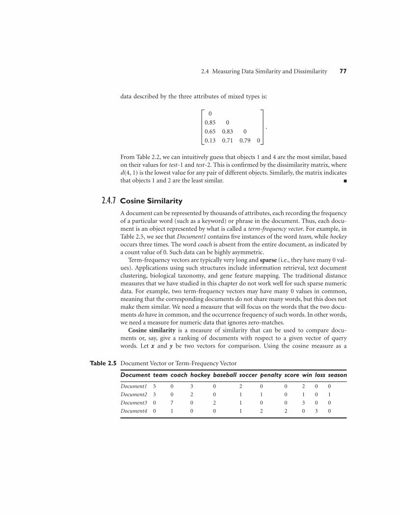
2.4 Measuring Data Similarity and Dissimilarity 77
data described by the three attributes of mixed types is:
⎡⎢⎢⎢⎣
0
0.85 0
0.65 0.83 0
0.13 0.71 0.79 0
⎤⎥⎥⎥⎦ .
From Table 2.2, we can intuitively guess that objects 1 and 4 are the most similar, basedon their values for test-1 and test-2. This is confirmed by the dissimilarity matrix, whered(4, 1) is the lowest value for any pair of different objects. Similarly, the matrix indicatesthat objects 1 and 2 are the least similar.
2.4.7 Cosine Similarity
A document can be represented by thousands of attributes, each recording the frequencyof a particular word (such as a keyword) or phrase in the document. Thus, each docu-ment is an object represented by what is called a term-frequency vector. For example, inTable 2.5, we see that Document1 contains five instances of the word team, while hockeyoccurs three times. The word coach is absent from the entire document, as indicated bya count value of 0. Such data can be highly asymmetric.
Term-frequency vectors are typically very long and sparse (i.e., they have many 0 val-ues). Applications using such structures include information retrieval, text documentclustering, biological taxonomy, and gene feature mapping. The traditional distancemeasures that we have studied in this chapter do not work well for such sparse numericdata. For example, two term-frequency vectors may have many 0 values in common,meaning that the corresponding documents do not share many words, but this does notmake them similar. We need a measure that will focus on the words that the two docu-ments do have in common, and the occurrence frequency of such words. In other words,we need a measure for numeric data that ignores zero-matches.
Cosine similarity is a measure of similarity that can be used to compare docu-ments or, say, give a ranking of documents with respect to a given vector of querywords. Let x and y be two vectors for comparison. Using the cosine measure as a
Table 2.5 Document Vector or Term-Frequency Vector
Document team coach hockey baseball soccer penalty score win loss season
Document1 5 0 3 0 2 0 0 2 0 0
Document2 3 0 2 0 1 1 0 1 0 1
Document3 0 7 0 2 1 0 0 3 0 0
Document4 0 1 0 0 1 2 2 0 3 0

78 Chapter 2 Getting to Know Your Data
similarity function, we have
sim(x, y) = x · y||x||||y|| , (2.23)
where ||x|| is the Euclidean norm of vector x = (x1, x2, . . . , xp), defined as√x2
1 + x22 + ·· · + x2
p . Conceptually, it is the length of the vector. Similarly, ||y|| is the
Euclidean norm of vector y. The measure computes the cosine of the angle between vec-tors x and y. A cosine value of 0 means that the two vectors are at 90 degrees to eachother (orthogonal) and have no match. The closer the cosine value to 1, the smaller theangle and the greater the match between vectors. Note that because the cosine similaritymeasure does not obey all of the properties of Section 2.4.4 defining metric measures, itis referred to as a nonmetric measure.
Example 2.23 Cosine similarity between two term-frequency vectors. Suppose that x and y are thefirst two term-frequency vectors in Table 2.5. That is, x = (5,0,3,0,2,0,0,2,0,0) andy = (3,0,2,0,1,1,0,1,0,1). How similar are x and y? Using Eq. (2.23) to compute thecosine similarity between the two vectors, we get:
xt · y = 5 × 3 + 0 × 0 + 3 × 2 + 0 × 0 + 2 × 1 + 0 × 1 + 0 × 0 + 2 × 1
+ 0 × 0 + 0 × 1 = 25
||x|| =√
52 + 02 + 32 + 02 + 22 + 02 + 02 + 22 + 02 + 02 = 6.48
||y|| =√
32 + 02 + 22 + 02 + 12 + 12 + 02 + 12 + 02 + 12 = 4.12
sim(x, y) = 0.94
Therefore, if we were using the cosine similarity measure to compare these documents,they would be considered quite similar.
When attributes are binary-valued, the cosine similarity function can be interpretedin terms of shared features or attributes. Suppose an object x possesses the ith attributeif xi = 1. Then xt · y is the number of attributes possessed (i.e., shared) by both x andy, and |x||y| is the geometric mean of the number of attributes possessed by x and thenumber possessed by y. Thus, sim(x, y) is a measure of relative possession of commonattributes.
A simple variation of cosine similarity for the preceding scenario is
sim(x, y) = x · yx · x + y · y − x · y
, (2.24)
which is the ratio of the number of attributes shared by x and y to the number ofattributes possessed by x or y. This function, known as the Tanimoto coefficient orTanimoto distance, is frequently used in information retrieval and biology taxonomy.

2.6 Exercises 79
2.5 Summary
Data sets are made up of data objects. A data object represents an entity. Data objectsare described by attributes. Attributes can be nominal, binary, ordinal, or numeric.
The values of a nominal (or categorical) attribute are symbols or names of things,where each value represents some kind of category, code, or state.
Binary attributes are nominal attributes with only two possible states (such as 1 and0 or true and false). If the two states are equally important, the attribute is symmetric;otherwise it is asymmetric.
An ordinal attribute is an attribute with possible values that have a meaningful orderor ranking among them, but the magnitude between successive values is not known.
A numeric attribute is quantitative (i.e., it is a measurable quantity) representedin integer or real values. Numeric attribute types can be interval-scaled or ratio-scaled. The values of an interval-scaled attribute are measured in fixed and equalunits. Ratio-scaled attributes are numeric attributes with an inherent zero-point.Measurements are ratio-scaled in that we can speak of values as being an order ofmagnitude larger than the unit of measurement.
Basic statistical descriptions provide the analytical foundation for data preprocess-ing. The basic statistical measures for data summarization include mean, weightedmean, median, and mode for measuring the central tendency of data; and range, quan-tiles, quartiles, interquartile range, variance, and standard deviation for measuring thedispersion of data. Graphical representations (e.g., boxplots, quantile plots, quantile–quantile plots, histograms, and scatter plots) facilitate visual inspection of the data andare thus useful for data preprocessing and mining.
Data visualization techniques may be pixel-oriented, geometric-based, icon-based, orhierarchical. These methods apply to multidimensional relational data. Additionaltechniques have been proposed for the visualization of complex data, such as textand social networks.
Measures of object similarity and dissimilarity are used in data mining applicationssuch as clustering, outlier analysis, and nearest-neighbor classification. Such mea-sures of proximity can be computed for each attribute type studied in this chapter,or for combinations of such attributes. Examples include the Jaccard coefficient forasymmetric binary attributes and Euclidean, Manhattan, Minkowski, and supremumdistances for numeric attributes. For applications involving sparse numeric data vec-tors, such as term-frequency vectors, the cosine measure and the Tanimoto coefficientare often used in the assessment of similarity.
2.6 Exercises
2.1 Give three additional commonly used statistical measures that are not already illus-trated in this chapter for the characterization of data dispersion. Discuss how they canbe computed efficiently in large databases.

80 Chapter 2 Getting to Know Your Data
2.2 Suppose that the data for analysis includes the attribute age. The age values for the datatuples are (in increasing order) 13, 15, 16, 16, 19, 20, 20, 21, 22, 22, 25, 25, 25, 25, 30,33, 33, 35, 35, 35, 35, 36, 40, 45, 46, 52, 70.
(a) What is the mean of the data? What is the median?
(b) What is the mode of the data? Comment on the data’s modality (i.e., bimodal,trimodal, etc.).
(c) What is the midrange of the data?
(d) Can you find (roughly) the first quartile (Q1) and the third quartile (Q3) of the data?
(e) Give the five-number summary of the data.
(f) Show a boxplot of the data.
(g) How is a quantile–quantile plot different from a quantile plot?
2.3 Suppose that the values for a given set of data are grouped into intervals. The intervalsand corresponding frequencies are as follows:
age frequency
1–5 200
6–15 450
16–20 300
21–50 1500
51–80 700
81–110 44
Compute an approximate median value for the data.
2.4 Suppose that a hospital tested the age and body fat data for 18 randomly selected adultswith the following results:
age 23 23 27 27 39 41 47 49 50
%fat 9.5 26.5 7.8 17.8 31.4 25.9 27.4 27.2 31.2
age 52 54 54 56 57 58 58 60 61
%fat 34.6 42.5 28.8 33.4 30.2 34.1 32.9 41.2 35.7
(a) Calculate the mean, median, and standard deviation of age and %fat.
(b) Draw the boxplots for age and %fat.
(c) Draw a scatter plot and a q-q plot based on these two variables.
2.5 Briefly outline how to compute the dissimilarity between objects described by thefollowing:
(a) Nominal attributes
(b) Asymmetric binary attributes

2.7 Bibliographic Notes 81
(c) Numeric attributes
(d) Term-frequency vectors
2.6 Given two objects represented by the tuples (22, 1, 42, 10) and (20, 0, 36, 8):
(a) Compute the Euclidean distance between the two objects.
(b) Compute the Manhattan distance between the two objects.
(c) Compute the Minkowski distance between the two objects, using q = 3.
(d) Compute the supremum distance between the two objects.
2.7 The median is one of the most important holistic measures in data analysis. Pro-pose several methods for median approximation. Analyze their respective complexityunder different parameter settings and decide to what extent the real value can beapproximated. Moreover, suggest a heuristic strategy to balance between accuracy andcomplexity and then apply it to all methods you have given.
2.8 It is important to define or select similarity measures in data analysis. However, thereis no commonly accepted subjective similarity measure. Results can vary depending onthe similarity measures used. Nonetheless, seemingly different similarity measures maybe equivalent after some transformation.
Suppose we have the following 2-D data set:
A1 A2
x1 1.5 1.7
x2 2 1.9
x3 1.6 1.8
x4 1.2 1.5
x5 1.5 1.0
(a) Consider the data as 2-D data points. Given a new data point, x = (1.4,1.6) as aquery, rank the database points based on similarity with the query using Euclideandistance, Manhattan distance, supremum distance, and cosine similarity.
(b) Normalize the data set to make the norm of each data point equal to 1. Use Euclideandistance on the transformed data to rank the data points.
2.7 Bibliographic Notes
Methods for descriptive data summarization have been studied in the statistics literaturelong before the onset of computers. Good summaries of statistical descriptive data min-ing methods include Freedman, Pisani, and Purves [FPP07] and Devore [Dev95]. For

82 Chapter 2 Getting to Know Your Data
statistics-based visualization of data using boxplots, quantile plots, quantile–quantileplots, scatter plots, and loess curves, see Cleveland [Cle93].
Pioneering work on data visualization techniques is described in The Visual Dis-play of Quantitative Information [Tuf83], Envisioning Information [Tuf90], and VisualExplanations: Images and Quantities, Evidence and Narrative [Tuf97], all by Tufte, inaddition to Graphics and Graphic Information Processing by Bertin [Ber81], VisualizingData by Cleveland [Cle93], and Information Visualization in Data Mining and KnowledgeDiscovery edited by Fayyad, Grinstein, and Wierse [FGW01].
Major conferences and symposiums on visualization include ACM Human Factorsin Computing Systems (CHI), Visualization, and the International Symposium on Infor-mation Visualization. Research on visualization is also published in Transactions onVisualization and Computer Graphics, Journal of Computational and Graphical Statistics,and IEEE Computer Graphics and Applications.
Many graphical user interfaces and visualization tools have been developed and canbe found in various data mining products. Several books on data mining (e.g., DataMining Solutions by Westphal and Blaxton [WB98]) present many good examples andvisual snapshots. For a survey of visualization techniques, see “Visual techniques forexploring databases” by Keim [Kei97].
Similarity and distance measures among various variables have been introduced inmany textbooks that study cluster analysis, including Hartigan [Har75]; Jain and Dubes[JD88]; Kaufman and Rousseeuw [KR90]; and Arabie, Hubert, and de Soete [AHS96].Methods for combining attributes of different types into a single dissimilarity matrixwere introduced by Kaufman and Rousseeuw [KR90].

3Data Preprocessing
Today’s real-world databases are highly susceptible to noisy, missing, and inconsistent datadue to their typically huge size (often several gigabytes or more) and their likely originfrom multiple, heterogenous sources. Low-quality data will lead to low-quality miningresults. “How can the data be preprocessed in order to help improve the quality of the dataand, consequently, of the mining results? How can the data be preprocessed so as to improvethe efficiency and ease of the mining process?”
There are several data preprocessing techniques. Data cleaning can be applied toremove noise and correct inconsistencies in data. Data integration merges data frommultiple sources into a coherent data store such as a data warehouse. Data reductioncan reduce data size by, for instance, aggregating, eliminating redundant features, orclustering. Data transformations (e.g., normalization) may be applied, where data arescaled to fall within a smaller range like 0.0 to 1.0. This can improve the accuracy andefficiency of mining algorithms involving distance measurements. These techniques arenot mutually exclusive; they may work together. For example, data cleaning can involvetransformations to correct wrong data, such as by transforming all entries for a date fieldto a common format.
In Chapter 2, we learned about the different attribute types and how to use basicstatistical descriptions to study data characteristics. These can help identify erroneousvalues and outliers, which will be useful in the data cleaning and integration steps.Data processing techniques, when applied before mining, can substantially improve theoverall quality of the patterns mined and/or the time required for the actual mining.
In this chapter, we introduce the basic concepts of data preprocessing in Section 3.1.The methods for data preprocessing are organized into the following categories: datacleaning (Section 3.2), data integration (Section 3.3), data reduction (Section 3.4), anddata transformation (Section 3.5).
c© 2012 Elsevier Inc. All rights reserved.
Data Mining: Concepts and Techniques 83
84 Chapter 3 Data Preprocessing
3.1 Data Preprocessing: An Overview
This section presents an overview of data preprocessing. Section 3.1.1 illustrates themany elements defining data quality. This provides the incentive behind data prepro-cessing. Section 3.1.2 outlines the major tasks in data preprocessing.
3.1.1 Data Quality: Why Preprocess the Data?
Data have quality if they satisfy the requirements of the intended use. There are manyfactors comprising data quality, including accuracy, completeness, consistency, timeliness,believability, and interpretability.
Imagine that you are a manager at AllElectronics and have been charged with ana-lyzing the company’s data with respect to your branch’s sales. You immediately set outto perform this task. You carefully inspect the company’s database and data warehouse,identifying and selecting the attributes or dimensions (e.g., item, price, and units sold)to be included in your analysis. Alas! You notice that several of the attributes for varioustuples have no recorded value. For your analysis, you would like to include informa-tion as to whether each item purchased was advertised as on sale, yet you discover thatthis information has not been recorded. Furthermore, users of your database systemhave reported errors, unusual values, and inconsistencies in the data recorded for sometransactions. In other words, the data you wish to analyze by data mining techniques areincomplete (lacking attribute values or certain attributes of interest, or containing onlyaggregate data); inaccurate or noisy (containing errors, or values that deviate from theexpected); and inconsistent (e.g., containing discrepancies in the department codes usedto categorize items). Welcome to the real world!
This scenario illustrates three of the elements defining data quality: accuracy, com-pleteness, and consistency. Inaccurate, incomplete, and inconsistent data are common-place properties of large real-world databases and data warehouses. There are manypossible reasons for inaccurate data (i.e., having incorrect attribute values). The data col-lection instruments used may be faulty. There may have been human or computer errorsoccurring at data entry. Users may purposely submit incorrect data values for manda-tory fields when they do not wish to submit personal information (e.g., by choosingthe default value “January 1” displayed for birthday). This is known as disguised missingdata. Errors in data transmission can also occur. There may be technology limitationssuch as limited buffer size for coordinating synchronized data transfer and consump-tion. Incorrect data may also result from inconsistencies in naming conventions or datacodes, or inconsistent formats for input fields (e.g., date). Duplicate tuples also requiredata cleaning.
Incomplete data can occur for a number of reasons. Attributes of interest may notalways be available, such as customer information for sales transaction data. Other datamay not be included simply because they were not considered important at the timeof entry. Relevant data may not be recorded due to a misunderstanding or because ofequipment malfunctions. Data that were inconsistent with other recorded data may

3.1 Data Preprocessing: An Overview 85
have been deleted. Furthermore, the recording of the data history or modifications mayhave been overlooked. Missing data, particularly for tuples with missing values for someattributes, may need to be inferred.
Recall that data quality depends on the intended use of the data. Two different usersmay have very different assessments of the quality of a given database. For example, amarketing analyst may need to access the database mentioned before for a list of cus-tomer addresses. Some of the addresses are outdated or incorrect, yet overall, 80% ofthe addresses are accurate. The marketing analyst considers this to be a large customerdatabase for target marketing purposes and is pleased with the database’s accuracy,although, as sales manager, you found the data inaccurate.
Timeliness also affects data quality. Suppose that you are overseeing the distribu-tion of monthly sales bonuses to the top sales representatives at AllElectronics. Severalsales representatives, however, fail to submit their sales records on time at the end ofthe month. There are also a number of corrections and adjustments that flow in afterthe month’s end. For a period of time following each month, the data stored in thedatabase are incomplete. However, once all of the data are received, it is correct. The factthat the month-end data are not updated in a timely fashion has a negative impact onthe data quality.
Two other factors affecting data quality are believability and interpretability. Believ-ability reflects how much the data are trusted by users, while interpretability reflectshow easy the data are understood. Suppose that a database, at one point, had severalerrors, all of which have since been corrected. The past errors, however, had causedmany problems for sales department users, and so they no longer trust the data. Thedata also use many accounting codes, which the sales department does not know how tointerpret. Even though the database is now accurate, complete, consistent, and timely,sales department users may regard it as of low quality due to poor believability andinterpretability.
3.1.2 Major Tasks in Data Preprocessing
In this section, we look at the major steps involved in data preprocessing, namely, datacleaning, data integration, data reduction, and data transformation.
Data cleaning routines work to “clean” the data by filling in missing values, smooth-ing noisy data, identifying or removing outliers, and resolving inconsistencies. If usersbelieve the data are dirty, they are unlikely to trust the results of any data mining that hasbeen applied. Furthermore, dirty data can cause confusion for the mining procedure,resulting in unreliable output. Although most mining routines have some proceduresfor dealing with incomplete or noisy data, they are not always robust. Instead, they mayconcentrate on avoiding overfitting the data to the function being modeled. Therefore,a useful preprocessing step is to run your data through some data cleaning routines.Section 3.2 discusses methods for data cleaning.
Getting back to your task at AllElectronics, suppose that you would like to includedata from multiple sources in your analysis. This would involve integrating multipledatabases, data cubes, or files (i.e., data integration). Yet some attributes representing a

86 Chapter 3 Data Preprocessing
given concept may have different names in different databases, causing inconsistenciesand redundancies. For example, the attribute for customer identification may be referredto as customer id in one data store and cust id in another. Naming inconsistencies mayalso occur for attribute values. For example, the same first name could be registered as“Bill” in one database, “William” in another, and “B.” in a third. Furthermore, you sus-pect that some attributes may be inferred from others (e.g., annual revenue). Havinga large amount of redundant data may slow down or confuse the knowledge discov-ery process. Clearly, in addition to data cleaning, steps must be taken to help avoidredundancies during data integration. Typically, data cleaning and data integration areperformed as a preprocessing step when preparing data for a data warehouse. Addi-tional data cleaning can be performed to detect and remove redundancies that may haveresulted from data integration.
“Hmmm,” you wonder, as you consider your data even further. “The data set I haveselected for analysis is HUGE, which is sure to slow down the mining process. Is there away I can reduce the size of my data set without jeopardizing the data mining results?”Data reduction obtains a reduced representation of the data set that is much smaller involume, yet produces the same (or almost the same) analytical results. Data reductionstrategies include dimensionality reduction and numerosity reduction.
In dimensionality reduction, data encoding schemes are applied so as to obtain areduced or “compressed” representation of the original data. Examples include datacompression techniques (e.g., wavelet transforms and principal components analysis),attribute subset selection (e.g., removing irrelevant attributes), and attribute construction(e.g., where a small set of more useful attributes is derived from the original set).
In numerosity reduction, the data are replaced by alternative, smaller representa-tions using parametric models (e.g., regression or log-linear models) or nonparametricmodels (e.g., histograms, clusters, sampling, or data aggregation). Data reduction is thetopic of Section 3.4.
Getting back to your data, you have decided, say, that you would like to use a distance-based mining algorithm for your analysis, such as neural networks, nearest-neighborclassifiers, or clustering.1 Such methods provide better results if the data to be ana-lyzed have been normalized, that is, scaled to a smaller range such as [0.0, 1.0]. Yourcustomer data, for example, contain the attributes age and annual salary. The annualsalary attribute usually takes much larger values than age. Therefore, if the attributesare left unnormalized, the distance measurements taken on annual salary will generallyoutweigh distance measurements taken on age. Discretization and concept hierarchy gen-eration can also be useful, where raw data values for attributes are replaced by ranges orhigher conceptual levels. For example, raw values for age may be replaced by higher-levelconcepts, such as youth, adult, or senior.
Discretization and concept hierarchy generation are powerful tools for data min-ing in that they allow data mining at multiple abstraction levels. Normalization, data
1Neural networks and nearest-neighbor classifiers are described in Chapter 9, and clustering is discussedin Chapters 10 and 11.

3.2 Data Preprocessing: An Overview 87
discretization, and concept hierarchy generation are forms of data transformation.You soon realize such data transformation operations are additional data preprocessingprocedures that would contribute toward the success of the mining process. Dataintegration and data discretization are discussed in Sections 3.5.
Figure 3.1 summarizes the data preprocessing steps described here. Note that the pre-vious categorization is not mutually exclusive. For example, the removal of redundantdata may be seen as a form of data cleaning, as well as data reduction.
In summary, real-world data tend to be dirty, incomplete, and inconsistent. Data pre-processing techniques can improve data quality, thereby helping to improve the accuracyand efficiency of the subsequent mining process. Data preprocessing is an important stepin the knowledge discovery process, because quality decisions must be based on qual-ity data. Detecting data anomalies, rectifying them early, and reducing the data to beanalyzed can lead to huge payoffs for decision making.
Data cleaning
Data integration
Data reductionAttributes Attributes
A1 A2 A3 ... A126
T1T2T3T4...T2000
Tra
nsac
tions
Tra
nsac
tions T1
T4...T1456
A1 A3 ... A115
Data transformation �2, 32, 100, 59, 48 �0.02, 0.32, 1.00, 0.59, 0.48
Figure 3.1 Forms of data preprocessing.

88 Chapter 3 Data Preprocessing
3.2 Data Cleaning
Real-world data tend to be incomplete, noisy, and inconsistent. Data cleaning (or datacleansing) routines attempt to fill in missing values, smooth out noise while identi-fying outliers, and correct inconsistencies in the data. In this section, you will studybasic methods for data cleaning. Section 3.2.1 looks at ways of handling missing values.Section 3.2.2 explains data smoothing techniques. Section 3.2.3 discusses approaches todata cleaning as a process.
3.2.1 Missing Values
Imagine that you need to analyze AllElectronics sales and customer data. You note thatmany tuples have no recorded value for several attributes such as customer income. Howcan you go about filling in the missing values for this attribute? Let’s look at the followingmethods.
1. Ignore the tuple: This is usually done when the class label is missing (assuming themining task involves classification). This method is not very effective, unless the tuplecontains several attributes with missing values. It is especially poor when the percent-age of missing values per attribute varies considerably. By ignoring the tuple, we donot make use of the remaining attributes’ values in the tuple. Such data could havebeen useful to the task at hand.
2. Fill in the missing value manually: In general, this approach is time consuming andmay not be feasible given a large data set with many missing values.
3. Use a global constant to fill in the missing value: Replace all missing attribute valuesby the same constant such as a label like “Unknown” or −∞. If missing values arereplaced by, say, “Unknown,” then the mining program may mistakenly think thatthey form an interesting concept, since they all have a value in common—that of“Unknown.” Hence, although this method is simple, it is not foolproof.
4. Use a measure of central tendency for the attribute (e.g., the mean or median) tofill in the missing value: Chapter 2 discussed measures of central tendency, whichindicate the “middle” value of a data distribution. For normal (symmetric) data dis-tributions, the mean can be used, while skewed data distribution should employthe median (Section 2.2). For example, suppose that the data distribution regard-ing the income of AllElectronics customers is symmetric and that the mean income is$56,000. Use this value to replace the missing value for income.
5. Use the attribute mean or median for all samples belonging to the same class asthe given tuple: For example, if classifying customers according to credit risk, wemay replace the missing value with the mean income value for customers in the samecredit risk category as that of the given tuple. If the data distribution for a given classis skewed, the median value is a better choice.
6. Use the most probable value to fill in the missing value: This may be determinedwith regression, inference-based tools using a Bayesian formalism, or decision tree

3.2 Data Cleaning 89
induction. For example, using the other customer attributes in your data set, youmay construct a decision tree to predict the missing values for income. Decision treesand Bayesian inference are described in detail in Chapters 8 and 9, respectively, whileregression is introduced in Section 3.4.5.
Methods 3 through 6 bias the data—the filled-in value may not be correct. Method 6,however, is a popular strategy. In comparison to the other methods, it uses the mostinformation from the present data to predict missing values. By considering the otherattributes’ values in its estimation of the missing value for income, there is a greaterchance that the relationships between income and the other attributes are preserved.
It is important to note that, in some cases, a missing value may not imply an errorin the data! For example, when applying for a credit card, candidates may be asked tosupply their driver’s license number. Candidates who do not have a driver’s license maynaturally leave this field blank. Forms should allow respondents to specify values suchas “not applicable.” Software routines may also be used to uncover other null values(e.g., “don’t know,” “?” or “none”). Ideally, each attribute should have one or more rulesregarding the null condition. The rules may specify whether or not nulls are allowedand/or how such values should be handled or transformed. Fields may also be inten-tionally left blank if they are to be provided in a later step of the business process. Hence,although we can try our best to clean the data after it is seized, good database and dataentry procedure design should help minimize the number of missing values or errors inthe first place.
3.2.2 Noisy Data
“What is noise?” Noise is a random error or variance in a measured variable. InChapter 2, we saw how some basic statistical description techniques (e.g., boxplotsand scatter plots), and methods of data visualization can be used to identify outliers,which may represent noise. Given a numeric attribute such as, say, price, how can we“smooth” out the data to remove the noise? Let’s look at the following data smoothingtechniques.
Binning: Binning methods smooth a sorted data value by consulting its “neighbor-hood,” that is, the values around it. The sorted values are distributed into a numberof “buckets,” or bins. Because binning methods consult the neighborhood of values,they perform local smoothing. Figure 3.2 illustrates some binning techniques. In thisexample, the data for price are first sorted and then partitioned into equal-frequencybins of size 3 (i.e., each bin contains three values). In smoothing by bin means, eachvalue in a bin is replaced by the mean value of the bin. For example, the mean of thevalues 4, 8, and 15 in Bin 1 is 9. Therefore, each original value in this bin is replacedby the value 9.
Similarly, smoothing by bin medians can be employed, in which each bin valueis replaced by the bin median. In smoothing by bin boundaries, the minimum andmaximum values in a given bin are identified as the bin boundaries. Each bin valueis then replaced by the closest boundary value. In general, the larger the width, the

90 Chapter 3 Data Preprocessing
Sorted data for price (in dollars): 4, 8, 15, 21, 21, 24, 25, 28, 34
Partition into (equal-frequency) bins:
Bin 1: 4, 8, 15Bin 2: 21, 21, 24Bin 3: 25, 28, 34
Smoothing by bin means:
Bin 1: 9, 9, 9Bin 2: 22, 22, 22Bin 3: 29, 29, 29
Smoothing by bin boundaries:
Bin 1: 4, 4, 15Bin 2: 21, 21, 24Bin 3: 25, 25, 34
Figure 3.2 Binning methods for data smoothing.
greater the effect of the smoothing. Alternatively, bins may be equal width, where theinterval range of values in each bin is constant. Binning is also used as a discretizationtechnique and is further discussed in Section 3.5.
Regression: Data smoothing can also be done by regression, a technique that con-forms data values to a function. Linear regression involves finding the “best” line tofit two attributes (or variables) so that one attribute can be used to predict the other.Multiple linear regression is an extension of linear regression, where more than twoattributes are involved and the data are fit to a multidimensional surface. Regressionis further described in Section 3.4.5.
Outlier analysis: Outliers may be detected by clustering, for example, where similarvalues are organized into groups, or “clusters.” Intuitively, values that fall outside ofthe set of clusters may be considered outliers (Figure 3.3). Chapter 12 is dedicated tothe topic of outlier analysis.
Many data smoothing methods are also used for data discretization (a form of datatransformation) and data reduction. For example, the binning techniques describedbefore reduce the number of distinct values per attribute. This acts as a form of datareduction for logic-based data mining methods, such as decision tree induction, whichrepeatedly makes value comparisons on sorted data. Concept hierarchies are a form ofdata discretization that can also be used for data smoothing. A concept hierarchy forprice, for example, may map real price values into inexpensive, moderately priced, andexpensive, thereby reducing the number of data values to be handled by the mining

3.2 Data Cleaning 91
Figure 3.3 A 2-D customer data plot with respect to customer locations in a city, showing three dataclusters. Outliers may be detected as values that fall outside of the cluster sets.
process. Data discretization is discussed in Section 3.5. Some methods of classification(e.g., neural networks) have built-in data smoothing mechanisms. Classification is thetopic of Chapters 8 and 9.
3.2.3 Data Cleaning as a Process
Missing values, noise, and inconsistencies contribute to inaccurate data. So far, we havelooked at techniques for handling missing data and for smoothing data. “But data clean-ing is a big job. What about data cleaning as a process? How exactly does one proceed intackling this task? Are there any tools out there to help?”
The first step in data cleaning as a process is discrepancy detection. Discrepancies canbe caused by several factors, including poorly designed data entry forms that have manyoptional fields, human error in data entry, deliberate errors (e.g., respondents not want-ing to divulge information about themselves), and data decay (e.g., outdated addresses).Discrepancies may also arise from inconsistent data representations and inconsistent useof codes. Other sources of discrepancies include errors in instrumentation devices thatrecord data and system errors. Errors can also occur when the data are (inadequately)used for purposes other than originally intended. There may also be inconsistencies dueto data integration (e.g., where a given attribute can have different names in differentdatabases).2
2Data integration and the removal of redundant data that can result from such integration are furtherdescribed in Section 3.3.

92 Chapter 3 Data Preprocessing
“So, how can we proceed with discrepancy detection?” As a starting point, use anyknowledge you may already have regarding properties of the data. Such knowledge or“data about data” is referred to as metadata. This is where we can make use of the know-ledge we gained about our data in Chapter 2. For example, what are the data type anddomain of each attribute? What are the acceptable values for each attribute? The basicstatistical data descriptions discussed in Section 2.2 are useful here to grasp data trendsand identify anomalies. For example, find the mean, median, and mode values. Are thedata symmetric or skewed? What is the range of values? Do all values fall within theexpected range? What is the standard deviation of each attribute? Values that are morethan two standard deviations away from the mean for a given attribute may be flaggedas potential outliers. Are there any known dependencies between attributes? In this step,you may write your own scripts and/or use some of the tools that we discuss further later.From this, you may find noise, outliers, and unusual values that need investigation.
As a data analyst, you should be on the lookout for the inconsistent use of codes andany inconsistent data representations (e.g., “2010/12/25” and “25/12/2010” for date).Field overloading is another error source that typically results when developers squeezenew attribute definitions into unused (bit) portions of already defined attributes (e.g.,an unused bit of an attribute that has a value range that uses only, say, 31 out of32 bits).
The data should also be examined regarding unique rules, consecutive rules, and nullrules. A unique rule says that each value of the given attribute must be different fromall other values for that attribute. A consecutive rule says that there can be no miss-ing values between the lowest and highest values for the attribute, and that all valuesmust also be unique (e.g., as in check numbers). A null rule specifies the use of blanks,question marks, special characters, or other strings that may indicate the null condition(e.g., where a value for a given attribute is not available), and how such values shouldbe handled. As mentioned in Section 3.2.1, reasons for missing values may include(1) the person originally asked to provide a value for the attribute refuses and/or findsthat the information requested is not applicable (e.g., a license number attribute leftblank by nondrivers); (2) the data entry person does not know the correct value; or (3)the value is to be provided by a later step of the process. The null rule should specify howto record the null condition, for example, such as to store zero for numeric attributes, ablank for character attributes, or any other conventions that may be in use (e.g., entrieslike “don’t know” or “?” should be transformed to blank).
There are a number of different commercial tools that can aid in the discrepancydetection step. Data scrubbing tools use simple domain knowledge (e.g., knowledgeof postal addresses and spell-checking) to detect errors and make corrections in thedata. These tools rely on parsing and fuzzy matching techniques when cleaning datafrom multiple sources. Data auditing tools find discrepancies by analyzing the data todiscover rules and relationships, and detecting data that violate such conditions. Theyare variants of data mining tools. For example, they may employ statistical analysis tofind correlations, or clustering to identify outliers. They may also use the basic statisticaldata descriptions presented in Section 2.2.
Some data inconsistencies may be corrected manually using external references.For example, errors made at data entry may be corrected by performing a paper

3.3 Data Integration 93
trace. Most errors, however, will require data transformations. That is, once we finddiscrepancies, we typically need to define and apply (a series of) transformations tocorrect them.
Commercial tools can assist in the data transformation step. Data migration toolsallow simple transformations to be specified such as to replace the string “gender” by“sex.” ETL (extraction/transformation/loading) tools allow users to specify transformsthrough a graphical user interface (GUI). These tools typically support only a restrictedset of transforms so that, often, we may also choose to write custom scripts for this stepof the data cleaning process.
The two-step process of discrepancy detection and data transformation (to correctdiscrepancies) iterates. This process, however, is error-prone and time consuming. Sometransformations may introduce more discrepancies. Some nested discrepancies may onlybe detected after others have been fixed. For example, a typo such as “20010” in a yearfield may only surface once all date values have been converted to a uniform format.Transformations are often done as a batch process while the user waits without feedback.Only after the transformation is complete can the user go back and check that no newanomalies have been mistakenly created. Typically, numerous iterations are requiredbefore the user is satisfied. Any tuples that cannot be automatically handled by a giventransformation are typically written to a file without any explanation regarding the rea-soning behind their failure. As a result, the entire data cleaning process also suffers froma lack of interactivity.
New approaches to data cleaning emphasize increased interactivity. Potter’s Wheel,for example, is a publicly available data cleaning tool that integrates discrepancy detec-tion and transformation. Users gradually build a series of transformations by composingand debugging individual transformations, one step at a time, on a spreadsheet-likeinterface. The transformations can be specified graphically or by providing examples.Results are shown immediately on the records that are visible on the screen. The usercan choose to undo the transformations, so that transformations that introduced addi-tional errors can be “erased.” The tool automatically performs discrepancy checking inthe background on the latest transformed view of the data. Users can gradually developand refine transformations as discrepancies are found, leading to more effective andefficient data cleaning.
Another approach to increased interactivity in data cleaning is the development ofdeclarative languages for the specification of data transformation operators. Such workfocuses on defining powerful extensions to SQL and algorithms that enable users toexpress data cleaning specifications efficiently.
As we discover more about the data, it is important to keep updating the metadatato reflect this knowledge. This will help speed up data cleaning on future versions of thesame data store.
3.3 Data Integration
Data mining often requires data integration—the merging of data from multiple datastores. Careful integration can help reduce and avoid redundancies and inconsistencies

94 Chapter 3 Data Preprocessing
in the resulting data set. This can help improve the accuracy and speed of the subsequentdata mining process.
The semantic heterogeneity and structure of data pose great challenges in data inte-gration. How can we match schema and objects from different sources? This is theessence of the entity identification problem, described in Section 3.3.1. Are any attributescorrelated? Section 3.3.2 presents correlation tests for numeric and nominal data. Tupleduplication is described in Section 3.3.3. Finally, Section 3.3.4 touches on the detectionand resolution of data value conflicts.
3.3.1 Entity Identification Problem
It is likely that your data analysis task will involve data integration, which combines datafrom multiple sources into a coherent data store, as in data warehousing. These sourcesmay include multiple databases, data cubes, or flat files.
There are a number of issues to consider during data integration. Schema integrationand object matching can be tricky. How can equivalent real-world entities from multipledata sources be matched up? This is referred to as the entity identification problem.For example, how can the data analyst or the computer be sure that customer id in onedatabase and cust number in another refer to the same attribute? Examples of metadatafor each attribute include the name, meaning, data type, and range of values permittedfor the attribute, and null rules for handling blank, zero, or null values (Section 3.2).Such metadata can be used to help avoid errors in schema integration. The metadatamay also be used to help transform the data (e.g., where data codes for pay type in onedatabase may be “H” and “S” but 1 and 2 in another). Hence, this step also relates todata cleaning, as described earlier.
When matching attributes from one database to another during integration, specialattention must be paid to the structure of the data. This is to ensure that any attributefunctional dependencies and referential constraints in the source system match those inthe target system. For example, in one system, a discount may be applied to the order,whereas in another system it is applied to each individual line item within the order.If this is not caught before integration, items in the target system may be improperlydiscounted.
3.3.2 Redundancy and Correlation Analysis
Redundancy is another important issue in data integration. An attribute (such as annualrevenue, for instance) may be redundant if it can be “derived” from another attributeor set of attributes. Inconsistencies in attribute or dimension naming can also causeredundancies in the resulting data set.
Some redundancies can be detected by correlation analysis. Given two attributes,such analysis can measure how strongly one attribute implies the other, based on theavailable data. For nominal data, we use the χ2 (chi-square) test. For numeric attributes,we can use the correlation coefficient and covariance, both of which access how oneattribute’s values vary from those of another.

3.3 Data Integration 95
χ2 Correlation Test for Nominal DataFor nominal data, a correlation relationship between two attributes, A and B, can bediscovered by a χ2 (chi-square) test. Suppose A has c distinct values, namely a1,a2, . . .ac .B has r distinct values, namely b1,b2, . . .br . The data tuples described by A and B can beshown as a contingency table, with the c values of A making up the columns and the rvalues of B making up the rows. Let (Ai ,Bj) denote the joint event that attribute A takeson value ai and attribute B takes on value bj , that is, where (A = ai ,B = bj). Each andevery possible (Ai ,Bj) joint event has its own cell (or slot) in the table. The χ2 value(also known as the Pearson χ2 statistic) is computed as
χ2 =c∑
i=1
r∑j=1
(oij − eij)2
eij, (3.1)
where oij is the observed frequency (i.e., actual count) of the joint event (Ai ,Bj) and eij isthe expected frequency of (Ai ,Bj), which can be computed as
eij = count(A = ai) × count(B = bj)
n, (3.2)
where n is the number of data tuples, count(A = ai) is the number of tuples having valueai for A, and count(B = bj) is the number of tuples having value bj for B. The sum inEq. (3.1) is computed over all of the r × c cells. Note that the cells that contribute themost to the χ2 value are those for which the actual count is very different from thatexpected.
The χ2 statistic tests the hypothesis that A and B are independent, that is, there is nocorrelation between them. The test is based on a significance level, with (r − 1) × (c − 1)
degrees of freedom. We illustrate the use of this statistic in Example 3.1. If the hypothesiscan be rejected, then we say that A and B are statistically correlated.
Example 3.1 Correlation analysis of nominal attributes using χ2. Suppose that a group of 1500people was surveyed. The gender of each person was noted. Each person was polled asto whether his or her preferred type of reading material was fiction or nonfiction. Thus,we have two attributes, gender and preferred reading. The observed frequency (or count)of each possible joint event is summarized in the contingency table shown in Table 3.1,where the numbers in parentheses are the expected frequencies. The expected frequen-cies are calculated based on the data distribution for both attributes using Eq. (3.2).
Using Eq. (3.2), we can verify the expected frequencies for each cell. For example,the expected frequency for the cell (male, fiction) is
e11 = count(male)× count(fiction)
n= 300 × 450
1500= 90,
and so on. Notice that in any row, the sum of the expected frequencies must equal thetotal observed frequency for that row, and the sum of the expected frequencies in anycolumn must also equal the total observed frequency for that column.

96 Chapter 3 Data Preprocessing
Table 3.1 Example 2.1’s 2 × 2 Contingency Table Data
male female Total
fiction 250 (90) 200 (360) 450
non fiction 50 (210) 1000 (840) 1050
Total 300 1200 1500
Note: Are gender and preferred reading correlated?
Using Eq. (3.1) for χ2 computation, we get
χ2 = (250 − 90)2
90+ (50 − 210)2
210+ (200 − 360)2
360+ (1000 − 840)2
840
= 284.44 + 121.90 + 71.11 + 30.48 = 507.93.
For this 2 × 2 table, the degrees of freedom are (2 − 1)(2 − 1) = 1. For 1 degree of free-dom, the χ2 value needed to reject the hypothesis at the 0.001 significance level is 10.828(taken from the table of upper percentage points of the χ2 distribution, typically avail-able from any textbook on statistics). Since our computed value is above this, we canreject the hypothesis that gender and preferred reading are independent and concludethat the two attributes are (strongly) correlated for the given group of people.
Correlation Coefficient for Numeric DataFor numeric attributes, we can evaluate the correlation between two attributes, A and B,by computing the correlation coefficient (also known as Pearson’s product momentcoefficient, named after its inventer, Karl Pearson). This is
rA,B =
n∑i=1
(ai − A)(bi − B)
nσAσB=
n∑i=1
(aibi) − nAB
nσAσB, (3.3)
where n is the number of tuples, ai and bi are the respective values of A and B in tuple i,A and B are the respective mean values of A and B, σA and σB are the respective standarddeviations of A and B (as defined in Section 2.2.2), and �(aibi) is the sum of the ABcross-product (i.e., for each tuple, the value for A is multiplied by the value for B in thattuple). Note that −1 ≤ rA,B ≤ +1. If rA,B is greater than 0, then A and B are positivelycorrelated, meaning that the values of A increase as the values of B increase. The higherthe value, the stronger the correlation (i.e., the more each attribute implies the other).Hence, a higher value may indicate that A (or B) may be removed as a redundancy.
If the resulting value is equal to 0, then A and B are independent and there is nocorrelation between them. If the resulting value is less than 0, then A and B are negativelycorrelated, where the values of one attribute increase as the values of the other attributedecrease. This means that each attribute discourages the other. Scatter plots can also beused to view correlations between attributes (Section 2.2.3). For example, Figure 2.8’s

3.3 Data Integration 97
scatter plots respectively show positively correlated data and negatively correlated data,while Figure 2.9 displays uncorrelated data.
Note that correlation does not imply causality. That is, if A and B are correlated, thisdoes not necessarily imply that A causes B or that B causes A. For example, in analyzing ademographic database, we may find that attributes representing the number of hospitalsand the number of car thefts in a region are correlated. This does not mean that onecauses the other. Both are actually causally linked to a third attribute, namely, population.
Covariance of Numeric DataIn probability theory and statistics, correlation and covariance are two similar measuresfor assessing how much two attributes change together. Consider two numeric attributesA and B, and a set of n observations {(a1,b1), . . . ,(an,bn)}. The mean values of A and B,respectively, are also known as the expected values on A and B, that is,
E(A) = A =∑n
i=1 ai
n
and
E(B) = B =∑n
i=1 bi
n.
The covariance between A and B is defined as
Cov(A,B) = E((A − A)(B − B)) =∑n
i=1(ai − A)(bi − B)
n. (3.4)
If we compare Eq. (3.3) for rA,B (correlation coefficient) with Eq. (3.4) for covariance,we see that
rA,B = Cov(A,B)
σAσB, (3.5)
where σA and σB are the standard deviations of A and B, respectively. It can also beshown that
Cov(A,B) = E(A · B) − AB. (3.6)
This equation may simplify calculations.For two attributes A and B that tend to change together, if A is larger than A (the
expected value of A), then B is likely to be larger than B (the expected value of B).Therefore, the covariance between A and B is positive. On the other hand, if one ofthe attributes tends to be above its expected value when the other attribute is below itsexpected value, then the covariance of A and B is negative.
If A and B are independent (i.e., they do not have correlation), then E(A · B) = E(A) ·E(B). Therefore, the covariance is Cov(A,B) = E(A · B) − AB = E(A) · E(B) − AB = 0.However, the converse is not true. Some pairs of random variables (attributes) may havea covariance of 0 but are not independent. Only under some additional assumptions

98 Chapter 3 Data Preprocessing
Table 3.2 Stock Prices for AllElectronics and HighTech
Time point AllElectronics HighTech
t1 6 20
t2 5 10
t3 4 14
t4 3 5
t5 2 5
(e.g., the data follow multivariate normal distributions) does a covariance of 0 implyindependence.
Example 3.2 Covariance analysis of numeric attributes. Consider Table 3.2, which presents a sim-plified example of stock prices observed at five time points for AllElectronics andHighTech, a high-tech company. If the stocks are affected by the same industry trends,will their prices rise or fall together?
E(AllElectronics) = 6 + 5 + 4 + 3 + 2
5= 20
5= $4
and
E(HighTech) = 20 + 10 + 14 + 5 + 5
5= 54
5= $10.80.
Thus, using Eq. (3.4), we compute
Cov(AllElectroncis,HighTech) = 6 × 20 + 5 × 10 + 4 × 14 + 3 × 5 + 2 × 5
5− 4 × 10.80
= 50.2 − 43.2 = 7.
Therefore, given the positive covariance we can say that stock prices for both companiesrise together.
Variance is a special case of covariance, where the two attributes are identical (i.e., thecovariance of an attribute with itself). Variance was discussed in Chapter 2.
3.3.3 Tuple Duplication
In addition to detecting redundancies between attributes, duplication should also bedetected at the tuple level (e.g., where there are two or more identical tuples for a givenunique data entry case). The use of denormalized tables (often done to improve per-formance by avoiding joins) is another source of data redundancy. Inconsistencies oftenarise between various duplicates, due to inaccurate data entry or updating some but notall data occurrences. For example, if a purchase order database contains attributes for

3.4 Data Reduction 99
the purchaser’s name and address instead of a key to this information in a purchaserdatabase, discrepancies can occur, such as the same purchaser’s name appearing withdifferent addresses within the purchase order database.
3.3.4 Data Value Conflict Detection and Resolution
Data integration also involves the detection and resolution of data value conflicts. Forexample, for the same real-world entity, attribute values from different sources may dif-fer. This may be due to differences in representation, scaling, or encoding. For instance,a weight attribute may be stored in metric units in one system and British imperialunits in another. For a hotel chain, the price of rooms in different cities may involvenot only different currencies but also different services (e.g., free breakfast) and taxes.When exchanging information between schools, for example, each school may have itsown curriculum and grading scheme. One university may adopt a quarter system, offerthree courses on database systems, and assign grades from A+ to F, whereas anothermay adopt a semester system, offer two courses on databases, and assign grades from 1to 10. It is difficult to work out precise course-to-grade transformation rules betweenthe two universities, making information exchange difficult.
Attributes may also differ on the abstraction level, where an attribute in one sys-tem is recorded at, say, a lower abstraction level than the “same” attribute in another.For example, the total sales in one database may refer to one branch of All Electronics,while an attribute of the same name in another database may refer to the total salesfor All Electronics stores in a given region. The topic of discrepancy detection is furtherdescribed in Section 3.2.3 on data cleaning as a process.
3.4 Data Reduction
Imagine that you have selected data from the AllElectronics data warehouse for analysis.The data set will likely be huge! Complex data analysis and mining on huge amounts ofdata can take a long time, making such analysis impractical or infeasible.
Data reduction techniques can be applied to obtain a reduced representation of thedata set that is much smaller in volume, yet closely maintains the integrity of the originaldata. That is, mining on the reduced data set should be more efficient yet produce thesame (or almost the same) analytical results. In this section, we first present an overviewof data reduction strategies, followed by a closer look at individual techniques.
3.4.1 Overview of Data Reduction Strategies
Data reduction strategies include dimensionality reduction, numerosity reduction, anddata compression.
Dimensionality reduction is the process of reducing the number of random variablesor attributes under consideration. Dimensionality reduction methods include wavelet

100 Chapter 3 Data Preprocessing
transforms (Section 3.4.2) and principal components analysis (Section 3.4.3), whichtransform or project the original data onto a smaller space. Attribute subset selection is amethod of dimensionality reduction in which irrelevant, weakly relevant, or redundantattributes or dimensions are detected and removed (Section 3.4.4).
Numerosity reduction techniques replace the original data volume by alternative,smaller forms of data representation. These techniques may be parametric or non-parametric. For parametric methods, a model is used to estimate the data, so thattypically only the data parameters need to be stored, instead of the actual data. (Out-liers may also be stored.) Regression and log-linear models (Section 3.4.5) are examples.Nonparametric methods for storing reduced representations of the data include his-tograms (Section 3.4.6), clustering (Section 3.4.7), sampling (Section 3.4.8), and datacube aggregation (Section 3.4.9).
In data compression, transformations are applied so as to obtain a reduced or “com-pressed” representation of the original data. If the original data can be reconstructedfrom the compressed data without any information loss, the data reduction is calledlossless. If, instead, we can reconstruct only an approximation of the original data, thenthe data reduction is called lossy. There are several lossless algorithms for string com-pression; however, they typically allow only limited data manipulation. Dimensionalityreduction and numerosity reduction techniques can also be considered forms of datacompression.
There are many other ways of organizing methods of data reduction. The computa-tional time spent on data reduction should not outweigh or “erase” the time saved bymining on a reduced data set size.
3.4.2 Wavelet Transforms
The discrete wavelet transform (DWT) is a linear signal processing technique that,when applied to a data vector X, transforms it to a numerically different vector, X′, ofwavelet coefficients. The two vectors are of the same length. When applying this tech-nique to data reduction, we consider each tuple as an n-dimensional data vector, thatis, X = (x1,x2, . . . ,xn), depicting n measurements made on the tuple from n databaseattributes.3
“How can this technique be useful for data reduction if the wavelet transformed data areof the same length as the original data?” The usefulness lies in the fact that the wavelettransformed data can be truncated. A compressed approximation of the data can beretained by storing only a small fraction of the strongest of the wavelet coefficients.For example, all wavelet coefficients larger than some user-specified threshold can beretained. All other coefficients are set to 0. The resulting data representation is thereforevery sparse, so that operations that can take advantage of data sparsity are computa-tionally very fast if performed in wavelet space. The technique also works to removenoise without smoothing out the main features of the data, making it effective for data
3In our notation, any variable representing a vector is shown in bold italic font; measurements depictingthe vector are shown in italic font.

3.4 Data Reduction 101
cleaning as well. Given a set of coefficients, an approximation of the original data can beconstructed by applying the inverse of the DWT used.
The DWT is closely related to the discrete Fourier transform (DFT), a signal process-ing technique involving sines and cosines. In general, however, the DWT achieves betterlossy compression. That is, if the same number of coefficients is retained for a DWT anda DFT of a given data vector, the DWT version will provide a more accurate approxima-tion of the original data. Hence, for an equivalent approximation, the DWT requires lessspace than the DFT. Unlike the DFT, wavelets are quite localized in space, contributingto the conservation of local detail.
There is only one DFT, yet there are several families of DWTs. Figure 3.4 showssome wavelet families. Popular wavelet transforms include the Haar-2, Daubechies-4,and Daubechies-6. The general procedure for applying a discrete wavelet transform usesa hierarchical pyramid algorithm that halves the data at each iteration, resulting in fastcomputational speed. The method is as follows:
1. The length, L, of the input data vector must be an integer power of 2. This conditioncan be met by padding the data vector with zeros as necessary (L ≥ n).
2. Each transform involves applying two functions. The first applies some data smooth-ing, such as a sum or weighted average. The second performs a weighted difference,which acts to bring out the detailed features of the data.
3. The two functions are applied to pairs of data points in X, that is, to all pairs ofmeasurements (x2i,x2i+1). This results in two data sets of length L/2. In general,these represent a smoothed or low-frequency version of the input data and the high-frequency content of it, respectively.
4. The two functions are recursively applied to the data sets obtained in the previousloop, until the resulting data sets obtained are of length 2.
5. Selected values from the data sets obtained in the previous iterations are designatedthe wavelet coefficients of the transformed data.
0 2 4 6
0.8
0.6
0.4
0.2
0.0
�1.0 �0.5 0.0 0.5(a) Haar-2 (b) Daubechies-4
1.0 1.5 2.0
0.6
0.4
0.2
0.0
Figure 3.4 Examples of wavelet families. The number next to a wavelet name is the number of vanishingmoments of the wavelet. This is a set of mathematical relationships that the coefficients mustsatisfy and is related to the number of coefficients.

102 Chapter 3 Data Preprocessing
Equivalently, a matrix multiplication can be applied to the input data in order toobtain the wavelet coefficients, where the matrix used depends on the given DWT. Thematrix must be orthonormal, meaning that the columns are unit vectors and are mutu-ally orthogonal, so that the matrix inverse is just its transpose. Although we do not haveroom to discuss it here, this property allows the reconstruction of the data from thesmooth and smooth-difference data sets. By factoring the matrix used into a product ofa few sparse matrices, the resulting “fast DWT” algorithm has a complexity of O(n) foran input vector of length n.
Wavelet transforms can be applied to multidimensional data such as a data cube. Thisis done by first applying the transform to the first dimension, then to the second, and soon. The computational complexity involved is linear with respect to the number of cellsin the cube. Wavelet transforms give good results on sparse or skewed data and on datawith ordered attributes. Lossy compression by wavelets is reportedly better than JPEGcompression, the current commercial standard. Wavelet transforms have many real-world applications, including the compression of fingerprint images, computer vision,analysis of time-series data, and data cleaning.
3.4.3 Principal Components Analysis
In this subsection we provide an intuitive introduction to principal components analy-sis as a method of dimesionality reduction. A detailed theoretical explanation is beyondthe scope of this book. For additional references, please see the bibliographic notes(Section 3.8) at the end of this chapter.
Suppose that the data to be reduced consist of tuples or data vectors describedby n attributes or dimensions. Principal components analysis (PCA; also called theKarhunen-Loeve, or K-L, method) searches for k n-dimensional orthogonal vectors thatcan best be used to represent the data, where k ≤ n. The original data are thus projectedonto a much smaller space, resulting in dimensionality reduction. Unlike attribute sub-set selection (Section 3.4.4), which reduces the attribute set size by retaining a subset ofthe initial set of attributes, PCA “combines” the essence of attributes by creating an alter-native, smaller set of variables. The initial data can then be projected onto this smallerset. PCA often reveals relationships that were not previously suspected and therebyallows interpretations that would not ordinarily result.
The basic procedure is as follows:
1. The input data are normalized, so that each attribute falls within the same range. Thisstep helps ensure that attributes with large domains will not dominate attributes withsmaller domains.
2. PCA computes k orthonormal vectors that provide a basis for the normalized inputdata. These are unit vectors that each point in a direction perpendicular to the others.These vectors are referred to as the principal components. The input data are a linearcombination of the principal components.
3. The principal components are sorted in order of decreasing “significance” orstrength. The principal components essentially serve as a new set of axes for the data,

3.4 Data Reduction 103
X2
X1
Y1Y2
Figure 3.5 Principal components analysis. Y1 and Y2 are the first two principal components for thegiven data.
providing important information about variance. That is, the sorted axes are suchthat the first axis shows the most variance among the data, the second axis shows thenext highest variance, and so on. For example, Figure 3.5 shows the first two princi-pal components, Y1 and Y2, for the given set of data originally mapped to the axes X1
and X2. This information helps identify groups or patterns within the data.
4. Because the components are sorted in decreasing order of “significance,” the data sizecan be reduced by eliminating the weaker components, that is, those with low vari-ance. Using the strongest principal components, it should be possible to reconstructa good approximation of the original data.
PCA can be applied to ordered and unordered attributes, and can handle sparse dataand skewed data. Multidimensional data of more than two dimensions can be han-dled by reducing the problem to two dimensions. Principal components may be usedas inputs to multiple regression and cluster analysis. In comparison with wavelet trans-forms, PCA tends to be better at handling sparse data, whereas wavelet transforms aremore suitable for data of high dimensionality.
3.4.4 Attribute Subset Selection
Data sets for analysis may contain hundreds of attributes, many of which may be irrel-evant to the mining task or redundant. For example, if the task is to classify customersbased on whether or not they are likely to purchase a popular new CD at AllElectronicswhen notified of a sale, attributes such as the customer’s telephone number are likely tobe irrelevant, unlike attributes such as age or music taste. Although it may be possible fora domain expert to pick out some of the useful attributes, this can be a difficult and time-consuming task, especially when the data’s behavior is not well known. (Hence, a reasonbehind its analysis!) Leaving out relevant attributes or keeping irrelevant attributes maybe detrimental, causing confusion for the mining algorithm employed. This can resultin discovered patterns of poor quality. In addition, the added volume of irrelevant orredundant attributes can slow down the mining process.

104 Chapter 3 Data Preprocessing
Attribute subset selection4 reduces the data set size by removing irrelevant orredundant attributes (or dimensions). The goal of attribute subset selection is to finda minimum set of attributes such that the resulting probability distribution of the dataclasses is as close as possible to the original distribution obtained using all attributes.Mining on a reduced set of attributes has an additional benefit: It reduces the numberof attributes appearing in the discovered patterns, helping to make the patterns easier tounderstand.
“How can we find a ‘good’ subset of the original attributes?” For n attributes, there are2n possible subsets. An exhaustive search for the optimal subset of attributes can be pro-hibitively expensive, especially as n and the number of data classes increase. Therefore,heuristic methods that explore a reduced search space are commonly used for attributesubset selection. These methods are typically greedy in that, while searching throughattribute space, they always make what looks to be the best choice at the time. Theirstrategy is to make a locally optimal choice in the hope that this will lead to a globallyoptimal solution. Such greedy methods are effective in practice and may come close toestimating an optimal solution.
The “best” (and “worst”) attributes are typically determined using tests of statisticalsignificance, which assume that the attributes are independent of one another. Manyother attribute evaluation measures can be used such as the information gain measureused in building decision trees for classification.5
Basic heuristic methods of attribute subset selection include the techniques thatfollow, some of which are illustrated in Figure 3.6.
Forward selection
Initial attribute set:{A1, A2, A3, A4, A5, A6}
Initial reduced set:{}=> {A1}=> {A1, A4}=> Reduced attribute set: {A1, A4, A6}
Initial attribute set:{A1, A2, A3, A4, A5, A6}
=> {A1, A3, A4, A5, A6}=> {A1, A4, A5, A6}=> Reduced attribute set: {A1, A4, A6}
Initial attribute set:{A1, A2, A3, A4, A5, A6}
=> Reduced attribute set: {A1, A4, A6}
Backward elimination Decision tree induction
A4?
A1? A6?
Class 1 Class 2 Class 1 Class 2
Y N
Y N Y N
Figure 3.6 Greedy (heuristic) methods for attribute subset selection.
4In machine learning, attribute subset selection is known as feature subset selection.5The information gain measure is described in detail in Chapter 8.
3.4 Data Reduction 105
1. Stepwise forward selection: The procedure starts with an empty set of attributes asthe reduced set. The best of the original attributes is determined and added to thereduced set. At each subsequent iteration or step, the best of the remaining originalattributes is added to the set.
2. Stepwise backward elimination: The procedure starts with the full set of attributes.At each step, it removes the worst attribute remaining in the set.
3. Combination of forward selection and backward elimination: The stepwise for-ward selection and backward elimination methods can be combined so that, at eachstep, the procedure selects the best attribute and removes the worst from among theremaining attributes.
4. Decision tree induction: Decision tree algorithms (e.g., ID3, C4.5, and CART) wereoriginally intended for classification. Decision tree induction constructs a flowchart-like structure where each internal (nonleaf) node denotes a test on an attribute, eachbranch corresponds to an outcome of the test, and each external (leaf) node denotes aclass prediction. At each node, the algorithm chooses the “best” attribute to partitionthe data into individual classes.
When decision tree induction is used for attribute subset selection, a tree is con-structed from the given data. All attributes that do not appear in the tree are assumedto be irrelevant. The set of attributes appearing in the tree form the reduced subsetof attributes.
The stopping criteria for the methods may vary. The procedure may employ a thresholdon the measure used to determine when to stop the attribute selection process.
In some cases, we may want to create new attributes based on others. Such attributeconstruction6 can help improve accuracy and understanding of structure in high-dimensional data. For example, we may wish to add the attribute area based on theattributes height and width. By combining attributes, attribute construction can dis-cover missing information about the relationships between data attributes that can beuseful for knowledge discovery.
3.4.5 Regression and Log-Linear Models: ParametricData Reduction
Regression and log-linear models can be used to approximate the given data. In (simple)linear regression, the data are modeled to fit a straight line. For example, a randomvariable, y (called a response variable), can be modeled as a linear function of anotherrandom variable, x (called a predictor variable), with the equation
y = wx + b, (3.7)
where the variance of y is assumed to be constant. In the context of data mining, x and yare numeric database attributes. The coefficients, w and b (called regression coefficients),
6In the machine learning literature, attribute construction is known as feature construction.

106 Chapter 3 Data Preprocessing
specify the slope of the line and the y-intercept, respectively. These coefficients canbe solved for by the method of least squares, which minimizes the error between theactual line separating the data and the estimate of the line. Multiple linear regressionis an extension of (simple) linear regression, which allows a response variable, y, to bemodeled as a linear function of two or more predictor variables.
Log-linear models approximate discrete multidimensional probability distributions.Given a set of tuples in n dimensions (e.g., described by n attributes), we can con-sider each tuple as a point in an n-dimensional space. Log-linear models can be usedto estimate the probability of each point in a multidimensional space for a set of dis-cretized attributes, based on a smaller subset of dimensional combinations. This allowsa higher-dimensional data space to be constructed from lower-dimensional spaces.Log-linear models are therefore also useful for dimensionality reduction (since thelower-dimensional points together typically occupy less space than the original datapoints) and data smoothing (since aggregate estimates in the lower-dimensional spaceare less subject to sampling variations than the estimates in the higher-dimensionalspace).
Regression and log-linear models can both be used on sparse data, although theirapplication may be limited. While both methods can handle skewed data, regressiondoes exceptionally well. Regression can be computationally intensive when applied tohigh-dimensional data, whereas log-linear models show good scalability for up to 10 orso dimensions.
Several software packages exist to solve regression problems. Examples include SAS(www.sas.com), SPSS (www.spss.com), and S-Plus (www.insightful.com). Another usefulresource is the book Numerical Recipes in C, by Press, Teukolsky, Vetterling, and Flannery[PTVF07], and its associated source code.
3.4.6 Histograms
Histograms use binning to approximate data distributions and are a popular formof data reduction. Histograms were introduced in Section 2.2.3. A histogram for anattribute, A, partitions the data distribution of A into disjoint subsets, referred to asbuckets or bins. If each bucket represents only a single attribute–value/frequency pair, thebuckets are called singleton buckets. Often, buckets instead represent continuous rangesfor the given attribute.
Example 3.3 Histograms. The following data are a list of AllElectronics prices for commonly solditems (rounded to the nearest dollar). The numbers have been sorted: 1, 1, 5, 5, 5,5, 5, 8, 8, 10, 10, 10, 10, 12, 14, 14, 14, 15, 15, 15, 15, 15, 15, 18, 18, 18, 18, 18,18, 18, 18, 20, 20, 20, 20, 20, 20, 20, 21, 21, 21, 21, 25, 25, 25, 25, 25, 28, 28, 30,30, 30.
Figure 3.7 shows a histogram for the data using singleton buckets. To further reducethe data, it is common to have each bucket denote a continuous value range forthe given attribute. In Figure 3.8, each bucket represents a different $10 range forprice.

3.4 Data Reduction 107
5 10
10
9
8
7
6
5
4
3
2
1
015 20 25 30
price ($)
coun
t
Figure 3.7 A histogram for price using singleton buckets—each bucket represents one price–value/frequency pair.
1–10 11–20 21–30
price ($)
coun
t
25
20
15
10
5
0
Figure 3.8 An equal-width histogram for price, where values are aggregated so that each bucket has auniform width of $10.
“How are the buckets determined and the attribute values partitioned?” There areseveral partitioning rules, including the following:
Equal-width: In an equal-width histogram, the width of each bucket range isuniform (e.g., the width of $10 for the buckets in Figure 3.8).
Equal-frequency (or equal-depth): In an equal-frequency histogram, the buckets arecreated so that, roughly, the frequency of each bucket is constant (i.e., each bucketcontains roughly the same number of contiguous data samples).

108 Chapter 3 Data Preprocessing
Histograms are highly effective at approximating both sparse and dense data, aswell as highly skewed and uniform data. The histograms described before for singleattributes can be extended for multiple attributes. Multidimensional histograms can cap-ture dependencies between attributes. These histograms have been found effective inapproximating data with up to five attributes. More studies are needed regarding theeffectiveness of multidimensional histograms for high dimensionalities.
Singleton buckets are useful for storing high-frequency outliers.
3.4.7 Clustering
Clustering techniques consider data tuples as objects. They partition the objects intogroups, or clusters, so that objects within a cluster are “similar” to one another and “dis-similar” to objects in other clusters. Similarity is commonly defined in terms of how“close” the objects are in space, based on a distance function. The “quality” of a clustermay be represented by its diameter, the maximum distance between any two objects inthe cluster. Centroid distance is an alternative measure of cluster quality and is definedas the average distance of each cluster object from the cluster centroid (denoting the“average object,” or average point in space for the cluster). Figure 3.3 showed a 2-D plotof customer data with respect to customer locations in a city. Three data clusters arevisible.
In data reduction, the cluster representations of the data are used to replace the actualdata. The effectiveness of this technique depends on the data’s nature. It is much moreeffective for data that can be organized into distinct clusters than for smeared data.
There are many measures for defining clusters and cluster quality. Clustering meth-ods are further described in Chapters 10 and 11.
3.4.8 Sampling
Sampling can be used as a data reduction technique because it allows a large data set tobe represented by a much smaller random data sample (or subset). Suppose that a largedata set, D, contains N tuples. Let’s look at the most common ways that we could sampleD for data reduction, as illustrated in Figure 3.9.
Simple random sample without replacement (SRSWOR) of size s: This is createdby drawing s of the N tuples from D (s < N), where the probability of drawing anytuple in D is 1/N , that is, all tuples are equally likely to be sampled.
Simple random sample with replacement (SRSWR) of size s: This is similar toSRSWOR, except that each time a tuple is drawn from D, it is recorded and thenreplaced. That is, after a tuple is drawn, it is placed back in D so that it may be drawnagain.
Cluster sample: If the tuples in D are grouped into M mutually disjoint “clusters,”then an SRS of s clusters can be obtained, where s < M . For example, tuples in adatabase are usually retrieved a page at a time, so that each page can be considered

3.4 Data Reduction 109
Cluster sample
Startified sample
Figure 3.9 Sampling can be used for data reduction.
a cluster. A reduced data representation can be obtained by applying, say, SRSWORto the pages, resulting in a cluster sample of the tuples. Other clustering criteria con-veying rich semantics can also be explored. For example, in a spatial database, wemay choose to define clusters geographically based on how closely different areas arelocated.
Stratified sample: If D is divided into mutually disjoint parts called strata, a stratifiedsample of D is generated by obtaining an SRS at each stratum. This helps ensure a

110 Chapter 3 Data Preprocessing
representative sample, especially when the data are skewed. For example, a stratifiedsample may be obtained from customer data, where a stratum is created for each cus-tomer age group. In this way, the age group having the smallest number of customerswill be sure to be represented.
An advantage of sampling for data reduction is that the cost of obtaining a sampleis proportional to the size of the sample, s, as opposed to N , the data set size. Hence,sampling complexity is potentially sublinear to the size of the data. Other data reduc-tion techniques can require at least one complete pass through D. For a fixed samplesize, sampling complexity increases only linearly as the number of data dimensions,n, increases, whereas techniques using histograms, for example, increase exponentiallyin n.
When applied to data reduction, sampling is most commonly used to estimate theanswer to an aggregate query. It is possible (using the central limit theorem) to deter-mine a sufficient sample size for estimating a given function within a specified degreeof error. This sample size, s, may be extremely small in comparison to N . Sampling isa natural choice for the progressive refinement of a reduced data set. Such a set can befurther refined by simply increasing the sample size.
3.4.9 Data Cube Aggregation
Imagine that you have collected the data for your analysis. These data consist of theAllElectronics sales per quarter, for the years 2008 to 2010. You are, however, interestedin the annual sales (total per year), rather than the total per quarter. Thus, the data canbe aggregated so that the resulting data summarize the total sales per year instead of perquarter. This aggregation is illustrated in Figure 3.10. The resulting data set is smaller involume, without loss of information necessary for the analysis task.
Data cubes are discussed in detail in Chapter 4 on data warehousing and Chapter 5on data cube technology. We briefly introduce some concepts here. Data cubes store
Quarter
Year 2010
Sales
Q1Q2Q3Q4
$224,000$408,000$350,000$586,000
Quarter
Year 2009
Sales
Q1Q2Q3Q4
$224,000$408,000$350,000$586,000
Quarter
Year 2008
Sales
Q1Q2Q3Q4
$224,000$408,000$350,000$586,000
Year Sales
200820092010
$1,568,000$2,356,000$3,594,000
Figure 3.10 Sales data for a given branch of AllElectronics for the years 2008 through 2010. On the left,the sales are shown per quarter. On the right, the data are aggregated to provide the annualsales.

3.5 Data Transformation and Data Discretization 111
568
A
B
C
D
750
150
50
homeentertainment
computer
phone
security
2008 2009year
item
_typ
e
bran
ch
2010
Figure 3.11 A data cube for sales at AllElectronics.
multidimensional aggregated information. For example, Figure 3.11 shows a data cubefor multidimensional analysis of sales data with respect to annual sales per item typefor each AllElectronics branch. Each cell holds an aggregate data value, correspondingto the data point in multidimensional space. (For readability, only some cell values areshown.) Concept hierarchies may exist for each attribute, allowing the analysis of dataat multiple abstraction levels. For example, a hierarchy for branch could allow branchesto be grouped into regions, based on their address. Data cubes provide fast access toprecomputed, summarized data, thereby benefiting online analytical processing as wellas data mining.
The cube created at the lowest abstraction level is referred to as the base cuboid. Thebase cuboid should correspond to an individual entity of interest such as sales or cus-tomer. In other words, the lowest level should be usable, or useful for the analysis. A cubeat the highest level of abstraction is the apex cuboid. For the sales data in Figure 3.11,the apex cuboid would give one total—the total sales for all three years, for all itemtypes, and for all branches. Data cubes created for varying levels of abstraction are oftenreferred to as cuboids, so that a data cube may instead refer to a lattice of cuboids. Eachhigher abstraction level further reduces the resulting data size. When replying to datamining requests, the smallest available cuboid relevant to the given task should be used.This issue is also addressed in Chapter 4.
3.5 Data Transformation and Data Discretization
This section presents methods of data transformation. In this preprocessing step, thedata are transformed or consolidated so that the resulting mining process may be moreefficient, and the patterns found may be easier to understand. Data discretization, a formof data transformation, is also discussed.

112 Chapter 3 Data Preprocessing
3.5.1 Data Transformation Strategies Overview
In data transformation, the data are transformed or consolidated into forms appropriatefor mining. Strategies for data transformation include the following:
1. Smoothing, which works to remove noise from the data. Techniques include binning,regression, and clustering.
2. Attribute construction (or feature construction), where new attributes are con-structed and added from the given set of attributes to help the mining process.
3. Aggregation, where summary or aggregation operations are applied to the data. Forexample, the daily sales data may be aggregated so as to compute monthly and annualtotal amounts. This step is typically used in constructing a data cube for data analysisat multiple abstraction levels.
4. Normalization, where the attribute data are scaled so as to fall within a smaller range,such as −1.0 to 1.0, or 0.0 to 1.0.
5. Discretization, where the raw values of a numeric attribute (e.g., age) are replaced byinterval labels (e.g., 0–10, 11–20, etc.) or conceptual labels (e.g., youth, adult, senior).The labels, in turn, can be recursively organized into higher-level concepts, resultingin a concept hierarchy for the numeric attribute. Figure 3.12 shows a concept hierarchyfor the attribute price. More than one concept hierarchy can be defined for the sameattribute to accommodate the needs of various users.
6. Concept hierarchy generation for nominal data, where attributes such as street canbe generalized to higher-level concepts, like city or country. Many hierarchies fornominal attributes are implicit within the database schema and can be automaticallydefined at the schema definition level.
Recall that there is much overlap between the major data preprocessing tasks. The firstthree of these strategies were discussed earlier in this chapter. Smoothing is a form of
($600...$800] ($800...$1000]($400...$600]($200...$400]($0...$200]
($0...$1000]
($900...$1000]
($800...$900]
($700...$800]
($600...$700]
($500...$600]
($100...$200]
($400...$500]
($0...$100]
($200...$300]
($300...$400]
Figure 3.12 A concept hierarchy for the attribute price, where an interval ($X . . .$Y ] denotes the rangefrom $X (exclusive) to $Y (inclusive).

3.5 Data Transformation and Data Discretization 113
data cleaning and was addressed in Section 3.2.2. Section 3.2.3 on the data cleaningprocess also discussed ETL tools, where users specify transformations to correct datainconsistencies. Attribute construction and aggregation were discussed in Section 3.4on data reduction. In this section, we therefore concentrate on the latter three strategies.
Discretization techniques can be categorized based on how the discretization is per-formed, such as whether it uses class information or which direction it proceeds (i.e.,top-down vs. bottom-up). If the discretization process uses class information, then wesay it is supervised discretization. Otherwise, it is unsupervised. If the process starts by firstfinding one or a few points (called split points or cut points) to split the entire attributerange, and then repeats this recursively on the resulting intervals, it is called top-downdiscretization or splitting. This contrasts with bottom-up discretization or merging, whichstarts by considering all of the continuous values as potential split-points, removes someby merging neighborhood values to form intervals, and then recursively applies thisprocess to the resulting intervals.
Data discretization and concept hierarchy generation are also forms of data reduc-tion. The raw data are replaced by a smaller number of interval or concept labels. Thissimplifies the original data and makes the mining more efficient. The resulting patternsmined are typically easier to understand. Concept hierarchies are also useful for miningat multiple abstraction levels.
The rest of this section is organized as follows. First, normalization techniques arepresented in Section 3.5.2. We then describe several techniques for data discretization,each of which can be used to generate concept hierarchies for numeric attributes. Thetechniques include binning (Section 3.5.3) and histogram analysis (Section 3.5.4), aswell as cluster analysis, decision tree analysis, and correlation analysis (Section 3.5.5).Finally, Section 3.5.6 describes the automatic generation of concept hierarchies fornominal data.
3.5.2 Data Transformation by Normalization
The measurement unit used can affect the data analysis. For example, changing mea-surement units from meters to inches for height, or from kilograms to pounds for weight,may lead to very different results. In general, expressing an attribute in smaller units willlead to a larger range for that attribute, and thus tend to give such an attribute greatereffect or “weight.” To help avoid dependence on the choice of measurement units, thedata should be normalized or standardized. This involves transforming the data to fallwithin a smaller or common range such as [−1,1] or [0.0, 1.0]. (The terms standardizeand normalize are used interchangeably in data preprocessing, although in statistics, thelatter term also has other connotations.)
Normalizing the data attempts to give all attributes an equal weight. Normaliza-tion is particularly useful for classification algorithms involving neural networks ordistance measurements such as nearest-neighbor classification and clustering. If usingthe neural network backpropagation algorithm for classification mining (Chapter 9),normalizing the input values for each attribute measured in the training tuples will helpspeed up the learning phase. For distance-based methods, normalization helps prevent

114 Chapter 3 Data Preprocessing
attributes with initially large ranges (e.g., income) from outweighing attributes withinitially smaller ranges (e.g., binary attributes). It is also useful when given no priorknowledge of the data.
There are many methods for data normalization. We study min-max normalization,z-score normalization, and normalization by decimal scaling. For our discussion, let A bea numeric attribute with n observed values, v1,v2, . . . ,vn.
Min-max normalization performs a linear transformation on the original data. Sup-pose that minA and maxA are the minimum and maximum values of an attribute, A.Min-max normalization maps a value, vi , of A to v′
i in the range [new minA,new maxA]by computing
v′i = vi − minA
maxA − minA(new maxA − new minA) + new minA. (3.8)
Min-max normalization preserves the relationships among the original data values. Itwill encounter an “out-of-bounds” error if a future input case for normalization fallsoutside of the original data range for A.
Example 3.4 Min-max normalization. Suppose that the minimum and maximum values for theattribute income are $12,000 and $98,000, respectively. We would like to map incometo the range [0.0,1.0]. By min-max normalization, a value of $73,600 for income istransformed to 73,600−12,000
98,000−12,000 (1.0 − 0) + 0 = 0.716.
In z-score normalization (or zero-mean normalization), the values for an attribute,A, are normalized based on the mean (i.e., average) and standard deviation of A. A value,vi , of A is normalized to v′
i by computing
v′i = vi − A
σA, (3.9)
where A and σA are the mean and standard deviation, respectively, of attribute A. Themean and standard deviation were discussed in Section 2.2, where A = 1
n (v1 + v2 + ·· · +vn) and σA is computed as the square root of the variance of A (see Eq. (2.6)). Thismethod of normalization is useful when the actual minimum and maximum of attributeA are unknown, or when there are outliers that dominate the min-max normalization.
Example 3.5 z-score normalization. Suppose that the mean and standard deviation of the values forthe attribute income are $54,000 and $16,000, respectively. With z-score normalization,a value of $73,600 for income is transformed to 73,600−54,000
16,000 = 1.225.
A variation of this z-score normalization replaces the standard deviation of Eq. (3.9)by the mean absolute deviation of A. The mean absolute deviation of A, denoted sA, is
sA = 1
n(|v1 − A| + |v2 − A| + · · · + |vn − A|). (3.10)

3.5 Data Transformation and Data Discretization 115
Thus, z-score normalization using the mean absolute deviation is
v′i = vi − A
sA. (3.11)
The mean absolute deviation, sA, is more robust to outliers than the standard deviation,σA. When computing the mean absolute deviation, the deviations from the mean (i.e.,|xi − x|) are not squared; hence, the effect of outliers is somewhat reduced.
Normalization by decimal scaling normalizes by moving the decimal point of valuesof attribute A. The number of decimal points moved depends on the maximum absolutevalue of A. A value, vi , of A is normalized to v′
i by computing
v′i = vi
10j, (3.12)
where j is the smallest integer such that max(|v′i |) < 1.
Example 3.6 Decimal scaling. Suppose that the recorded values of A range from −986 to 917. Themaximum absolute value of A is 986. To normalize by decimal scaling, we thereforedivide each value by 1000 (i.e., j = 3) so that −986 normalizes to −0.986 and 917normalizes to 0.917.
Note that normalization can change the original data quite a bit, especially whenusing z-score normalization or decimal scaling. It is also necessary to save the normaliza-tion parameters (e.g., the mean and standard deviation if using z-score normalization)so that future data can be normalized in a uniform manner.
3.5.3 Discretization by Binning
Binning is a top-down splitting technique based on a specified number of bins.Section 3.2.2 discussed binning methods for data smoothing. These methods are alsoused as discretization methods for data reduction and concept hierarchy generation. Forexample, attribute values can be discretized by applying equal-width or equal-frequencybinning, and then replacing each bin value by the bin mean or median, as in smoothingby bin means or smoothing by bin medians, respectively. These techniques can be appliedrecursively to the resulting partitions to generate concept hierarchies.
Binning does not use class information and is therefore an unsupervised discretiza-tion technique. It is sensitive to the user-specified number of bins, as well as the presenceof outliers.
3.5.4 Discretization by Histogram Analysis
Like binning, histogram analysis is an unsupervised discretization technique because itdoes not use class information. Histograms were introduced in Section 2.2.3. A his-togram partitions the values of an attribute, A, into disjoint ranges called bucketsor bins.

116 Chapter 3 Data Preprocessing
Various partitioning rules can be used to define histograms (Section 3.4.6). In anequal-width histogram, for example, the values are partitioned into equal-size partitionsor ranges (e.g., earlier in Figure 3.8 for price, where each bucket has a width of $10).With an equal-frequency histogram, the values are partitioned so that, ideally, each par-tition contains the same number of data tuples. The histogram analysis algorithm can beapplied recursively to each partition in order to automatically generate a multilevel con-cept hierarchy, with the procedure terminating once a prespecified number of conceptlevels has been reached. A minimum interval size can also be used per level to control therecursive procedure. This specifies the minimum width of a partition, or the minimumnumber of values for each partition at each level. Histograms can also be partitionedbased on cluster analysis of the data distribution, as described next.
3.5.5 Discretization by Cluster, Decision Tree,and Correlation Analyses
Clustering, decision tree analysis, and correlation analysis can be used for data dis-cretization. We briefly study each of these approaches.
Cluster analysis is a popular data discretization method. A clustering algorithm canbe applied to discretize a numeric attribute, A, by partitioning the values of A into clus-ters or groups. Clustering takes the distribution of A into consideration, as well as thecloseness of data points, and therefore is able to produce high-quality discretizationresults.
Clustering can be used to generate a concept hierarchy for A by following either atop-down splitting strategy or a bottom-up merging strategy, where each cluster formsa node of the concept hierarchy. In the former, each initial cluster or partition maybe further decomposed into several subclusters, forming a lower level of the hiera-rchy. In the latter, clusters are formed by repeatedly grouping neighboring clusters inorder to form higher-level concepts. Clustering methods for data mining are studied inChapters 10 and 11.
Techniques to generate decision trees for classification (Chapter 8) can be applied todiscretization. Such techniques employ a top-down splitting approach. Unlike the othermethods mentioned so far, decision tree approaches to discretization are supervised,that is, they make use of class label information. For example, we may have a data set ofpatient symptoms (the attributes) where each patient has an associated diagnosis classlabel. Class distribution information is used in the calculation and determination ofsplit-points (data values for partitioning an attribute range). Intuitively, the main ideais to select split-points so that a given resulting partition contains as many tuples of thesame class as possible. Entropy is the most commonly used measure for this purpose. Todiscretize a numeric attribute, A, the method selects the value of A that has the minimumentropy as a split-point, and recursively partitions the resulting intervals to arrive at ahierarchical discretization. Such discretization forms a concept hierarchy for A.
Because decision tree–based discretization uses class information, it is more likelythat the interval boundaries (split-points) are defined to occur in places that may helpimprove classification accuracy. Decision trees and the entropy measure are described ingreater detail in Section 8.2.2.

3.5 Data Transformation and Data Discretization 117
Measures of correlation can be used for discretization. ChiMerge is a χ2-baseddiscretization method. The discretization methods that we have studied up to thispoint have all employed a top-down, splitting strategy. This contrasts with ChiMerge,which employs a bottom-up approach by finding the best neighboring intervals andthen merging them to form larger intervals, recursively. As with decision tree analysis,ChiMerge is supervised in that it uses class information. The basic notion is that foraccurate discretization, the relative class frequencies should be fairly consistent withinan interval. Therefore, if two adjacent intervals have a very similar distribution of classes,then the intervals can be merged. Otherwise, they should remain separate.
ChiMerge proceeds as follows. Initially, each distinct value of a numeric attribute A isconsidered to be one interval. χ2 tests are performed for every pair of adjacent intervals.Adjacent intervals with the least χ2 values are merged together, because low χ2 valuesfor a pair indicate similar class distributions. This merging process proceeds recursivelyuntil a predefined stopping criterion is met.
3.5.6 Concept Hierarchy Generation for Nominal Data
We now look at data transformation for nominal data. In particular, we study concepthierarchy generation for nominal attributes. Nominal attributes have a finite (but pos-sibly large) number of distinct values, with no ordering among the values. Examplesinclude geographic location, job category, and item type.
Manual definition of concept hierarchies can be a tedious and time-consuming taskfor a user or a domain expert. Fortunately, many hierarchies are implicit within thedatabase schema and can be automatically defined at the schema definition level. Theconcept hierarchies can be used to transform the data into multiple levels of granular-ity. For example, data mining patterns regarding sales may be found relating to specificregions or countries, in addition to individual branch locations.
We study four methods for the generation of concept hierarchies for nominal data,as follows.
1. Specification of a partial ordering of attributes explicitly at the schema level byusers or experts: Concept hierarchies for nominal attributes or dimensions typicallyinvolve a group of attributes. A user or expert can easily define a concept hierarchy byspecifying a partial or total ordering of the attributes at the schema level. For exam-ple, suppose that a relational database contains the following group of attributes:street, city, province or state, and country. Similarly, a data warehouse location dimen-sion may contain the same attributes. A hierarchy can be defined by specifying thetotal ordering among these attributes at the schema level such as street < city <
province or state < country.
2. Specification of a portion of a hierarchy by explicit data grouping: This is essen-tially the manual definition of a portion of a concept hierarchy. In a large database,it is unrealistic to define an entire concept hierarchy by explicit value enumera-tion. On the contrary, we can easily specify explicit groupings for a small portionof intermediate-level data. For example, after specifying that province and country

118 Chapter 3 Data Preprocessing
form a hierarchy at the schema level, a user could define some intermediate levelsmanually, such as “{Alberta, Saskatchewan, Manitoba} ⊂ prairies Canada” and“{British Columbia, prairies Canada} ⊂ Western Canada.”
3. Specification of a set of attributes, but not of their partial ordering: A user mayspecify a set of attributes forming a concept hierarchy, but omit to explicitly statetheir partial ordering. The system can then try to automatically generate the attributeordering so as to construct a meaningful concept hierarchy.
“Without knowledge of data semantics, how can a hierarchical ordering for anarbitrary set of nominal attributes be found?” Consider the observation that sincehigher-level concepts generally cover several subordinate lower-level concepts, anattribute defining a high concept level (e.g., country) will usually contain a smallernumber of distinct values than an attribute defining a lower concept level (e.g.,street). Based on this observation, a concept hierarchy can be automatically gener-ated based on the number of distinct values per attribute in the given attribute set.The attribute with the most distinct values is placed at the lowest hierarchy level. Thelower the number of distinct values an attribute has, the higher it is in the gener-ated concept hierarchy. This heuristic rule works well in many cases. Some local-levelswapping or adjustments may be applied by users or experts, when necessary, afterexamination of the generated hierarchy.
Let’s examine an example of this third method.
Example 3.7 Concept hierarchy generation based on the number of distinct values per attribute.Suppose a user selects a set of location-oriented attributes—street, country, provinceor state, and city—from the AllElectronics database, but does not specify the hierarchicalordering among the attributes.
A concept hierarchy for location can be generated automatically, as illustrated inFigure 3.13. First, sort the attributes in ascending order based on the number of dis-tinct values in each attribute. This results in the following (where the number of distinctvalues per attribute is shown in parentheses): country (15), province or state (365), city(3567), and street (674,339). Second, generate the hierarchy from the top down accord-ing to the sorted order, with the first attribute at the top level and the last attribute at thebottom level. Finally, the user can examine the generated hierarchy, and when necessary,modify it to reflect desired semantic relationships among the attributes. In this example,it is obvious that there is no need to modify the generated hierarchy.
Note that this heuristic rule is not foolproof. For example, a time dimension in adatabase may contain 20 distinct years, 12 distinct months, and 7 distinct days of theweek. However, this does not suggest that the time hierarchy should be “year < month <
days of the week,” with days of the week at the top of the hierarchy.
4. Specification of only a partial set of attributes: Sometimes a user can be carelesswhen defining a hierarchy, or have only a vague idea about what should be includedin a hierarchy. Consequently, the user may have included only a small subset of the

3.5 Data Transformation and Data Discretization 119
country 15 distinct values
province_or_state
city
street
365 distinct values
3567 distinct values
674,339 distinct values
Figure 3.13 Automatic generation of a schema concept hierarchy based on the number of distinctattribute values.
relevant attributes in the hierarchy specification. For example, instead of includingall of the hierarchically relevant attributes for location, the user may have specifiedonly street and city. To handle such partially specified hierarchies, it is important toembed data semantics in the database schema so that attributes with tight semanticconnections can be pinned together. In this way, the specification of one attributemay trigger a whole group of semantically tightly linked attributes to be “dragged in”to form a complete hierarchy. Users, however, should have the option to override thisfeature, as necessary.
Example 3.8 Concept hierarchy generation using prespecified semantic connections. Suppose thata data mining expert (serving as an administrator) has pinned together the five attri-butes number, street, city, province or state, and country, because they are closely linkedsemantically regarding the notion of location. If a user were to specify only the attributecity for a hierarchy defining location, the system can automatically drag in all five seman-tically related attributes to form a hierarchy. The user may choose to drop any ofthese attributes (e.g., number and street) from the hierarchy, keeping city as the lowestconceptual level.
In summary, information at the schema level and on attribute–value counts can beused to generate concept hierarchies for nominal data. Transforming nominal data withthe use of concept hierarchies allows higher-level knowledge patterns to be found. Itallows mining at multiple levels of abstraction, which is a common requirement for datamining applications.

120 Chapter 3 Data Preprocessing
3.6 Summary
Data quality is defined in terms of accuracy, completeness, consistency, timeliness,believability, and interpretabilty. These qualities are assessed based on the intendeduse of the data.
Data cleaning routines attempt to fill in missing values, smooth out noise whileidentifying outliers, and correct inconsistencies in the data. Data cleaning is usuallyperformed as an iterative two-step process consisting of discrepancy detection anddata transformation.
Data integration combines data from multiple sources to form a coherent datastore. The resolution of semantic heterogeneity, metadata, correlation analysis,tuple duplication detection, and data conflict detection contribute to smooth dataintegration.
Data reduction techniques obtain a reduced representation of the data while mini-mizing the loss of information content. These include methods of dimensionalityreduction, numerosity reduction, and data compression. Dimensionality reductionreduces the number of random variables or attributes under consideration. Methodsinclude wavelet transforms, principal components analysis, attribute subset selection,and attribute creation. Numerosity reduction methods use parametric or nonparat-metric models to obtain smaller representations of the original data. Parametricmodels store only the model parameters instead of the actual data. Examplesinclude regression and log-linear models. Nonparamteric methods include his-tograms, clustering, sampling, and data cube aggregation. Data compression meth-ods apply transformations to obtain a reduced or “compressed” representation ofthe original data. The data reduction is lossless if the original data can be recon-structed from the compressed data without any loss of information; otherwise, it islossy.
Data transformation routines convert the data into appropriate forms for min-ing. For example, in normalization, attribute data are scaled so as to fall within asmall range such as 0.0 to 1.0. Other examples are data discretization and concepthierarchy generation.
Data discretization transforms numeric data by mapping values to interval or con-cept labels. Such methods can be used to automatically generate concept hierarchiesfor the data, which allows for mining at multiple levels of granularity. Discretiza-tion techniques include binning, histogram analysis, cluster analysis, decision treeanalysis, and correlation analysis. For nominal data, concept hierarchies may begenerated based on schema definitions as well as the number of distinct values perattribute.
Although numerous methods of data preprocessing have been developed, data pre-processing remains an active area of research, due to the huge amount of inconsistentor dirty data and the complexity of the problem.

3.7 Exercises 121
3.7 Exercises
3.1 Data quality can be assessed in terms of several issues, including accuracy, completeness,and consistency. For each of the above three issues, discuss how data quality assess-ment can depend on the intended use of the data, giving examples. Propose two otherdimensions of data quality.
3.2 In real-world data, tuples with missing values for some attributes are a commonoccurrence. Describe various methods for handling this problem.
3.3 Exercise 2.2 gave the following data (in increasing order) for the attribute age: 13, 15,16, 16, 19, 20, 20, 21, 22, 22, 25, 25, 25, 25, 30, 33, 33, 35, 35, 35, 35, 36, 40, 45, 46,52, 70.
(a) Use smoothing by bin means to smooth these data, using a bin depth of 3. Illustrateyour steps. Comment on the effect of this technique for the given data.
(b) How might you determine outliers in the data?
(c) What other methods are there for data smoothing?
3.4 Discuss issues to consider during data integration.
3.5 What are the value ranges of the following normalization methods?
(a) min-max normalization
(b) z-score normalization
(c) z-score normalization using the mean absolute deviation instead of standard devia-tion
(d) normalization by decimal scaling
3.6 Use these methods to normalize the following group of data:
200,300,400,600,1000
(a) min-max normalization by setting min = 0 and max = 1
(b) z-score normalization
(c) z-score normalization using the mean absolute deviation instead of standard devia-tion
(d) normalization by decimal scaling
3.7 Using the data for age given in Exercise 3.3, answer the following:
(a) Use min-max normalization to transform the value 35 for age onto the range[0.0,1.0].
(b) Use z-score normalization to transform the value 35 for age, where the standarddeviation of age is 12.94 years.
(c) Use normalization by decimal scaling to transform the value 35 for age.
(d) Comment on which method you would prefer to use for the given data, givingreasons as to why.

122 Chapter 3 Data Preprocessing
3.8 Using the data for age and body fat given in Exercise 2.4, answer the following:
(a) Normalize the two attributes based on z-score normalization.
(b) Calculate the correlation coefficient (Pearson’s product moment coefficient). Arethese two attributes positively or negatively correlated? Compute their covariance.
3.9 Suppose a group of 12 sales price records has been sorted as follows:
5,10,11,13,15,35,50,55,72,92,204,215.
Partition them into three bins by each of the following methods:
(a) equal-frequency (equal-depth) partitioning
(b) equal-width partitioning
(c) clustering
3.10 Use a flowchart to summarize the following procedures for attribute subset selection:
(a) stepwise forward selection
(b) stepwise backward elimination
(c) a combination of forward selection and backward elimination
3.11 Using the data for age given in Exercise 3.3,
(a) Plot an equal-width histogram of width 10.
(b) Sketch examples of each of the following sampling techniques: SRSWOR, SRSWR,cluster sampling, and stratified sampling. Use samples of size 5 and the strata“youth,” “middle-aged,” and “senior.”
3.12 ChiMerge [Ker92] is a supervised, bottom-up (i.e., merge-based) data discretizationmethod. It relies on χ2 analysis: Adjacent intervals with the least χ2 values are mergedtogether until the chosen stopping criterion satisfies.
(a) Briefly describe how ChiMerge works.
(b) Take the IRIS data set, obtained from the University of California–Irvine MachineLearning Data Repository (www.ics.uci.edu/∼mlearn/MLRepository.html), as a dataset to be discretized. Perform data discretization for each of the four numericattributes using the ChiMerge method. (Let the stopping criteria be: max-interval= 6). You need to write a small program to do this to avoid clumsy numericalcomputation. Submit your simple analysis and your test results: split-points, finalintervals, and the documented source program.
3.13 Propose an algorithm, in pseudocode or in your favorite programming language, for thefollowing:
(a) The automatic generation of a concept hierarchy for nominal data based on thenumber of distinct values of attributes in the given schema.
(b) The automatic generation of a concept hierarchy for numeric data based on theequal-width partitioning rule.

3.8 Bibliographic Notes 123
(c) The automatic generation of a concept hierarchy for numeric data based on theequal-frequency partitioning rule.
3.14 Robust data loading poses a challenge in database systems because the input data areoften dirty. In many cases, an input record may miss multiple values; some recordscould be contaminated, with some data values out of range or of a different data typethan expected. Work out an automated data cleaning and loading algorithm so that theerroneous data will be marked and contaminated data will not be mistakenly insertedinto the database during data loading.
3.8 Bibliographic Notes
Data preprocessing is discussed in a number of textbooks, including English [Eng99],Pyle [Pyl99], Loshin [Los01], Redman [Red01], and Dasu and Johnson [DJ03]. Morespecific references to individual preprocessing techniques are given later.
For discussion regarding data quality, see Redman [Red92]; Wang, Storey, andFirth [WSF95]; Wand and Wang [WW96]; Ballou and Tayi [BT99]; and Olson [Ols03].Potter’s Wheel (control.cx.berkely.edu/abc), the interactive data cleaning tool described inSection 3.2.3, is presented in Raman and Hellerstein [RH01]. An example of the devel-opment of declarative languages for the specification of data transformation operators isgiven in Galhardas et al. [GFS+01]. The handling of missing attribute values is discussedin Friedman [Fri77]; Breiman, Friedman, Olshen, and Stone [BFOS84]; and Quinlan[Qui89]. Hua and Pei [HP07] presented a heuristic approach to cleaning disguised miss-ing data, where such data are captured when users falsely select default values on forms(e.g., “January 1” for birthdate) when they do not want to disclose personal information.
A method for the detection of outlier or “garbage” patterns in a handwritten char-acter database is given in Guyon, Matic, and Vapnik [GMV96]. Binning and datanormalization are treated in many texts, including Kennedy et al. [KLV+98], Weissand Indurkhya [WI98], and Pyle [Pyl99]. Systems that include attribute (or feature)construction include BACON by Langley, Simon, Bradshaw, and Zytkow [LSBZ87];Stagger by Schlimmer [Sch86]; FRINGE by Pagallo [Pag89]; and AQ17-DCI by Bloe-dorn and Michalski [BM98]. Attribute construction is also described in Liu and Motoda[LM98a, LM98b]. Dasu et al. built a BELLMAN system and proposed a set of interestingmethods for building a data quality browser by mining database structures [DJMS02].
A good survey of data reduction techniques can be found in Barbara et al. [BDF+97].For algorithms on data cubes and their precomputation, see Sarawagi and Stonebraker[SS94]; Agarwal et al. [AAD+96]; Harinarayan, Rajaraman, and Ullman [HRU96]; Rossand Srivastava [RS97]; and Zhao, Deshpande, and Naughton [ZDN97]. Attribute sub-set selection (or feature subset selection) is described in many texts such as Neter, Kutner,Nachtsheim, and Wasserman [NKNW96]; Dash and Liu [DL97]; and Liu and Motoda[LM98a, LM98b]. A combination forward selection and backward elimination method

124 Chapter 3 Data Preprocessing
was proposed in Siedlecki and Sklansky [SS88]. A wrapper approach to attribute selec-tion is described in Kohavi and John [KJ97]. Unsupervised attribute subset selection isdescribed in Dash, Liu, and Yao [DLY97].
For a description of wavelets for dimensionality reduction, see Press, Teukolosky, Vet-terling, and Flannery [PTVF07]. A general account of wavelets can be found in Hubbard[Hub96]. For a list of wavelet software packages, see Bruce, Donoho, and Gao [BDG96].Daubechies transforms are described in Daubechies [Dau92]. The book by Press et al.[PTVF07] includes an introduction to singular value decomposition for principal com-ponents analysis. Routines for PCA are included in most statistical software packagessuch as SAS (www.sas.com/SASHome.html).
An introduction to regression and log-linear models can be found in severaltextbooks such as James [Jam85]; Dobson [Dob90]; Johnson and Wichern [JW92];Devore [Dev95]; and Neter, Kutner, Nachtsheim, and Wasserman [NKNW96]. For log-linear models (known as multiplicative models in the computer science literature), seePearl [Pea88]. For a general introduction to histograms, see Barbara et al. [BDF+97]and Devore and Peck [DP97]. For extensions of single-attribute histograms to multipleattributes, see Muralikrishna and DeWitt [MD88] and Poosala and Ioannidis [PI97].Several references to clustering algorithms are given in Chapters 10 and 11 of this book,which are devoted to the topic.
A survey of multidimensional indexing structures is given in Gaede and Gunther[GG98]. The use of multidimensional index trees for data aggregation is discussed inAoki [Aok98]. Index trees include R-trees (Guttman [Gut84]), quad-trees (Finkel andBentley [FB74]), and their variations. For discussion on sampling and data mining, seeKivinen and Mannila [KM94] and John and Langley [JL96].
There are many methods for assessing attribute relevance. Each has its own bias. Theinformation gain measure is biased toward attributes with many values. Many alterna-tives have been proposed, such as gain ratio (Quinlan [Qui93]), which considers theprobability of each attribute value. Other relevance measures include the Gini index(Breiman, Friedman, Olshen, and Stone [BFOS84]), the χ2 contingency table statis-tic, and the uncertainty coefficient (Johnson and Wichern [JW92]). For a comparisonof attribute selection measures for decision tree induction, see Buntine and Niblett[BN92]. For additional methods, see Liu and Motoda [LM98a], Dash and Liu [DL97],and Almuallim and Dietterich [AD91].
Liu et al. [LHTD02] performed a comprehensive survey of data discretizationmethods. Entropy-based discretization with the C4.5 algorithm is described in Quin-lan [Qui93]. In Catlett [Cat91], the D-2 system binarizes a numeric feature recursively.ChiMerge by Kerber [Ker92] and Chi2 by Liu and Setiono [LS95] are methods for theautomatic discretization of numeric attributes that both employ the χ2 statistic. Fayyadand Irani [FI93] apply the minimum description length principle to determine the num-ber of intervals for numeric discretization. Concept hierarchies and their automaticgeneration from categorical data are described in Han and Fu [HF94].

4Data Warehousing and OnlineAnalytical Processing
Data warehouses generalize and consolidate data in multidimensional space. The constructionof data warehouses involves data cleaning, data integration, and data transformation,and can be viewed as an important preprocessing step for data mining. Moreover, datawarehouses provide online analytical processing (OLAP) tools for the interactive analysisof multidimensional data of varied granularities, which facilitates effective data gene-ralization and data mining. Many other data mining functions, such as association,classification, prediction, and clustering, can be integrated with OLAP operations toenhance interactive mining of knowledge at multiple levels of abstraction. Hence, thedata warehouse has become an increasingly important platform for data analysis andOLAP and will provide an effective platform for data mining. Therefore, data warehous-ing and OLAP form an essential step in the knowledge discovery process. This chapterpresents an overview of data warehouse and OLAP technology. This overview is essentialfor understanding the overall data mining and knowledge discovery process.
In this chapter, we study a well-accepted definition of the data warehouse and seewhy more and more organizations are building data warehouses for the analysis oftheir data (Section 4.1). In particular, we study the data cube, a multidimensional datamodel for data warehouses and OLAP, as well as OLAP operations such as roll-up, drill-down, slicing, and dicing (Section 4.2). We also look at data warehouse design andusage (Section 4.3). In addition, we discuss multidimensional data mining, a power-ful paradigm that integrates data warehouse and OLAP technology with that of datamining. An overview of data warehouse implementation examines general strategiesfor efficient data cube computation, OLAP data indexing, and OLAP query process-ing (Section 4.4). Finally, we study data generalization by attribute-oriented induction(Section 4.5). This method uses concept hierarchies to generalize data to multiple levelsof abstraction.
4.1 Data Warehouse: Basic Concepts
This section gives an introduction to data warehouses. We begin with a definition of thedata warehouse (Section 4.1.1). We outline the differences between operational database
c© 2012 Elsevier Inc. All rights reserved.
Data Mining: Concepts and Techniques 125

126 Chapter 4 Data Warehousing and Online Analytical Processing
systems and data warehouses (Section 4.1.2), then explain the need for using data ware-houses for data analysis, rather than performing the analysis directly on traditionaldatabases (Section 4.1.3). This is followed by a presentation of data warehouse architec-ture (Section 4.1.4). Next, we study three data warehouse models—an enterprise model,a data mart, and a virtual warehouse (Section 4.1.5). Section 4.1.6 describes back-endutilities for data warehousing, such as extraction, transformation, and loading. Finally,Section 4.1.7 presents the metadata repository, which stores data about data.
4.1.1 What Is a Data Warehouse?
Data warehousing provides architectures and tools for business executives to system-atically organize, understand, and use their data to make strategic decisions. Datawarehouse systems are valuable tools in today’s competitive, fast-evolving world. In thelast several years, many firms have spent millions of dollars in building enterprise-widedata warehouses. Many people feel that with competition mounting in every industry,data warehousing is the latest must-have marketing weapon—a way to retain customersby learning more about their needs.
“Then, what exactly is a data warehouse?” Data warehouses have been defined in manyways, making it difficult to formulate a rigorous definition. Loosely speaking, a datawarehouse refers to a data repository that is maintained separately from an organiza-tion’s operational databases. Data warehouse systems allow for integration of a variety ofapplication systems. They support information processing by providing a solid platformof consolidated historic data for analysis.
According to William H. Inmon, a leading architect in the construction of datawarehouse systems, “A data warehouse is a subject-oriented, integrated, time-variant,and nonvolatile collection of data in support of management’s decision making pro-cess” [Inm96]. This short but comprehensive definition presents the major features ofa data warehouse. The four keywords—subject-oriented, integrated, time-variant, andnonvolatile—distinguish data warehouses from other data repository systems, such asrelational database systems, transaction processing systems, and file systems.
Let’s take a closer look at each of these key features.
Subject-oriented: A data warehouse is organized around major subjects such as cus-tomer, supplier, product, and sales. Rather than concentrating on the day-to-dayoperations and transaction processing of an organization, a data warehouse focuseson the modeling and analysis of data for decision makers. Hence, data warehousestypically provide a simple and concise view of particular subject issues by excludingdata that are not useful in the decision support process.
Integrated: A data warehouse is usually constructed by integrating multiple hetero-geneous sources, such as relational databases, flat files, and online transactionrecords. Data cleaning and data integration techniques are applied to ensure con-sistency in naming conventions, encoding structures, attribute measures, and so on.

4.1 Data Warehouse: Basic Concepts 127
Time-variant: Data are stored to provide information from an historic perspective(e.g., the past 5–10 years). Every key structure in the data warehouse contains, eitherimplicitly or explicitly, a time element.
Nonvolatile: A data warehouse is always a physically separate store of data trans-formed from the application data found in the operational environment. Due tothis separation, a data warehouse does not require transaction processing, recovery,and concurrency control mechanisms. It usually requires only two operations in dataaccessing: initial loading of data and access of data.
In sum, a data warehouse is a semantically consistent data store that serves as aphysical implementation of a decision support data model. It stores the informationan enterprise needs to make strategic decisions. A data warehouse is also often viewedas an architecture, constructed by integrating data from multiple heterogeneous sourcesto support structured and/or ad hoc queries, analytical reporting, and decision making.
Based on this information, we view data warehousing as the process of construct-ing and using data warehouses. The construction of a data warehouse requires datacleaning, data integration, and data consolidation. The utilization of a data warehouseoften necessitates a collection of decision support technologies. This allows “knowledgeworkers” (e.g., managers, analysts, and executives) to use the warehouse to quickly andconveniently obtain an overview of the data, and to make sound decisions based oninformation in the warehouse. Some authors use the term data warehousing to referonly to the process of data warehouse construction, while the term warehouse DBMS isused to refer to the management and utilization of data warehouses. We will not makethis distinction here.
“How are organizations using the information from data warehouses?” Many orga-nizations use this information to support business decision-making activities, includ-ing (1) increasing customer focus, which includes the analysis of customer buyingpatterns (such as buying preference, buying time, budget cycles, and appetites forspending); (2) repositioning products and managing product portfolios by compar-ing the performance of sales by quarter, by year, and by geographic regions in orderto fine-tune production strategies; (3) analyzing operations and looking for sources ofprofit; and (4) managing customer relationships, making environmental corrections,and managing the cost of corporate assets.
Data warehousing is also very useful from the point of view of heterogeneous databaseintegration. Organizations typically collect diverse kinds of data and maintain largedatabases from multiple, heterogeneous, autonomous, and distributed informationsources. It is highly desirable, yet challenging, to integrate such data and provide easyand efficient access to it. Much effort has been spent in the database industry andresearch community toward achieving this goal.
The traditional database approach to heterogeneous database integration is to buildwrappers and integrators (or mediators) on top of multiple, heterogeneous databases.When a query is posed to a client site, a metadata dictionary is used to translate thequery into queries appropriate for the individual heterogeneous sites involved. These

128 Chapter 4 Data Warehousing and Online Analytical Processing
queries are then mapped and sent to local query processors. The results returned fromthe different sites are integrated into a global answer set. This query-driven approachrequires complex information filtering and integration processes, and competes withlocal sites for processing resources. It is inefficient and potentially expensive for frequentqueries, especially queries requiring aggregations.
Data warehousing provides an interesting alternative to this traditional approach.Rather than using a query-driven approach, data warehousing employs an update-driven approach in which information from multiple, heterogeneous sources is inte-grated in advance and stored in a warehouse for direct querying and analysis. Unlikeonline transaction processing databases, data warehouses do not contain the most cur-rent information. However, a data warehouse brings high performance to the integratedheterogeneous database system because data are copied, preprocessed, integrated, anno-tated, summarized, and restructured into one semantic data store. Furthermore, queryprocessing in data warehouses does not interfere with the processing at local sources.Moreover, data warehouses can store and integrate historic information and supportcomplex multidimensional queries. As a result, data warehousing has become popularin industry.
4.1.2 Differences between Operational Database Systemsand Data Warehouses
Because most people are familiar with commercial relational database systems, it is easyto understand what a data warehouse is by comparing these two kinds of systems.
The major task of online operational database systems is to perform online trans-action and query processing. These systems are called online transaction processing(OLTP) systems. They cover most of the day-to-day operations of an organization suchas purchasing, inventory, manufacturing, banking, payroll, registration, and account-ing. Data warehouse systems, on the other hand, serve users or knowledge workers inthe role of data analysis and decision making. Such systems can organize and presentdata in various formats in order to accommodate the diverse needs of different users.These systems are known as online analytical processing (OLAP) systems.
The major distinguishing features of OLTP and OLAP are summarized as follows:
Users and system orientation: An OLTP system is customer-oriented and is usedfor transaction and query processing by clerks, clients, and information technologyprofessionals. An OLAP system is market-oriented and is used for data analysis byknowledge workers, including managers, executives, and analysts.
Data contents: An OLTP system manages current data that, typically, are too detailedto be easily used for decision making. An OLAP system manages large amounts ofhistoric data, provides facilities for summarization and aggregation, and stores andmanages information at different levels of granularity. These features make the dataeasier to use for informed decision making.

4.1 Data Warehouse: Basic Concepts 129
Database design: An OLTP system usually adopts an entity-relationship (ER) datamodel and an application-oriented database design. An OLAP system typicallyadopts either a star or a snowflake model (see Section 4.2.2) and a subject-orienteddatabase design.
View: An OLTP system focuses mainly on the current data within an enterprise ordepartment, without referring to historic data or data in different organizations. Incontrast, an OLAP system often spans multiple versions of a database schema, due tothe evolutionary process of an organization. OLAP systems also deal with informa-tion that originates from different organizations, integrating information from manydata stores. Because of their huge volume, OLAP data are stored on multiple storagemedia.
Access patterns: The access patterns of an OLTP system consist mainly of short,atomic transactions. Such a system requires concurrency control and recovery mech-anisms. However, accesses to OLAP systems are mostly read-only operations (becausemost data warehouses store historic rather than up-to-date information), althoughmany could be complex queries.
Other features that distinguish between OLTP and OLAP systems include databasesize, frequency of operations, and performance metrics. These are summarized inTable 4.1.
4.1.3 But, Why Have a Separate Data Warehouse?
Because operational databases store huge amounts of data, you may wonder, “Why notperform online analytical processing directly on such databases instead of spending addi-tional time and resources to construct a separate data warehouse?” A major reason for sucha separation is to help promote the high performance of both systems. An operationaldatabase is designed and tuned from known tasks and workloads like indexing andhashing using primary keys, searching for particular records, and optimizing “canned”queries. On the other hand, data warehouse queries are often complex. They involve thecomputation of large data groups at summarized levels, and may require the use of spe-cial data organization, access, and implementation methods based on multidimensionalviews. Processing OLAP queries in operational databases would substantially degradethe performance of operational tasks.
Moreover, an operational database supports the concurrent processing of multipletransactions. Concurrency control and recovery mechanisms (e.g., locking and logging)are required to ensure the consistency and robustness of transactions. An OLAP queryoften needs read-only access of data records for summarization and aggregation. Con-currency control and recovery mechanisms, if applied for such OLAP operations, mayjeopardize the execution of concurrent transactions and thus substantially reduce thethroughput of an OLTP system.
Finally, the separation of operational databases from data warehouses is based onthe different structures, contents, and uses of the data in these two systems. Decision

130 Chapter 4 Data Warehousing and Online Analytical Processing
Table 4.1 Comparison of OLTP and OLAP Systems
Feature OLTP OLAP
Characteristic operational processing informational processing
Orientation transaction analysis
User clerk, DBA, database professional knowledge worker (e.g., manager,executive, analyst)
Function day-to-day operations long-term informationalrequirements decision support
DB design ER-based, application-oriented star/snowflake, subject-oriented
Data current, guaranteed up-to-date historic, accuracy maintainedover time
Summarization primitive, highly detailed summarized, consolidated
View detailed, flat relational summarized, multidimensional
Unit of work short, simple transaction complex query
Access read/write mostly read
Focus data in information out
Operations index/hash on primary key lots of scans
Number of recordsaccessed tens millions
Number of users thousands hundreds
DB size GB to high-order GB ≥ TB
Priority high performance, high availability high flexibility, end-user autonomy
Metric transaction throughput query throughput, response time
Note: Table is partially based on Chaudhuri and Dayal [CD97].
support requires historic data, whereas operational databases do not typically maintainhistoric data. In this context, the data in operational databases, though abundant, areusually far from complete for decision making. Decision support requires consolidation(e.g., aggregation and summarization) of data from heterogeneous sources, resultingin high-quality, clean, integrated data. In contrast, operational databases contain onlydetailed raw data, such as transactions, which need to be consolidated before analy-sis. Because the two systems provide quite different functionalities and require differentkinds of data, it is presently necessary to maintain separate databases. However, manyvendors of operational relational database management systems are beginning to opti-mize such systems to support OLAP queries. As this trend continues, the separationbetween OLTP and OLAP systems is expected to decrease.
4.1.4 Data Warehousing: A Multitiered Architecture
Data warehouses often adopt a three-tier architecture, as presented in Figure 4.1.

4.1 Data Warehouse: Basic Concepts 131
Query/report Analysis Data mining
OLAP server OLAP server
Top tier:Front-end tools
Middle tier:OLAP server
Bottom tier:Data warehouseserver
Data
Output
ExtractClean
TransformLoad
Refresh
Data warehouse Data martsMonitoring
Metadata repository
Operational databases External sources
Administration
Figure 4.1 A three-tier data warehousing architecture.
1. The bottom tier is a warehouse database server that is almost always a relationaldatabase system. Back-end tools and utilities are used to feed data into the bot-tom tier from operational databases or other external sources (e.g., customer profileinformation provided by external consultants). These tools and utilities perform dataextraction, cleaning, and transformation (e.g., to merge similar data from differentsources into a unified format), as well as load and refresh functions to update thedata warehouse (see Section 4.1.6). The data are extracted using application pro-gram interfaces known as gateways. A gateway is supported by the underlying DBMSand allows client programs to generate SQL code to be executed at a server. Exam-ples of gateways include ODBC (Open Database Connection) and OLEDB (Object

132 Chapter 4 Data Warehousing and Online Analytical Processing
Linking and Embedding Database) by Microsoft and JDBC (Java Database Connec-tion). This tier also contains a metadata repository, which stores information aboutthe data warehouse and its contents. The metadata repository is further described inSection 4.1.7.
2. The middle tier is an OLAP server that is typically implemented using either (1) arelational OLAP (ROLAP) model (i.e., an extended relational DBMS that maps oper-ations on multidimensional data to standard relational operations); or (2) a multi-dimensional OLAP (MOLAP) model (i.e., a special-purpose server that directlyimplements multidimensional data and operations). OLAP servers are discussed inSection 4.4.4.
3. The top tier is a front-end client layer, which contains query and reporting tools,analysis tools, and/or data mining tools (e.g., trend analysis, prediction, and so on).
4.1.5 Data Warehouse Models: Enterprise Warehouse,Data Mart, and Virtual Warehouse
From the architecture point of view, there are three data warehouse models: theenterprise warehouse, the data mart, and the virtual warehouse.
Enterprise warehouse: An enterprise warehouse collects all of the information aboutsubjects spanning the entire organization. It provides corporate-wide data inte-gration, usually from one or more operational systems or external informationproviders, and is cross-functional in scope. It typically contains detailed data aswell as summarized data, and can range in size from a few gigabytes to hundredsof gigabytes, terabytes, or beyond. An enterprise data warehouse may be imple-mented on traditional mainframes, computer superservers, or parallel architectureplatforms. It requires extensive business modeling and may take years to designand build.
Data mart: A data mart contains a subset of corporate-wide data that is of value to aspecific group of users. The scope is confined to specific selected subjects. For exam-ple, a marketing data mart may confine its subjects to customer, item, and sales. Thedata contained in data marts tend to be summarized.
Data marts are usually implemented on low-cost departmental servers that areUnix/Linux or Windows based. The implementation cycle of a data mart is morelikely to be measured in weeks rather than months or years. However, it mayinvolve complex integration in the long run if its design and planning were notenterprise-wide.
Depending on the source of data, data marts can be categorized as independentor dependent. Independent data marts are sourced from data captured from one ormore operational systems or external information providers, or from data generatedlocally within a particular department or geographic area. Dependent data marts aresourced directly from enterprise data warehouses.

4.1 Data Warehouse: Basic Concepts 133
Virtual warehouse: A virtual warehouse is a set of views over operational databases.For efficient query processing, only some of the possible summary views may bematerialized. A virtual warehouse is easy to build but requires excess capacity onoperational database servers.
“What are the pros and cons of the top-down and bottom-up approaches to data ware-house development?” The top-down development of an enterprise warehouse serves as asystematic solution and minimizes integration problems. However, it is expensive, takesa long time to develop, and lacks flexibility due to the difficulty in achieving consistencyand consensus for a common data model for the entire organization. The bottom-up approach to the design, development, and deployment of independent data martsprovides flexibility, low cost, and rapid return of investment. It, however, can lead toproblems when integrating various disparate data marts into a consistent enterprise datawarehouse.
A recommended method for the development of data warehouse systems is to imple-ment the warehouse in an incremental and evolutionary manner, as shown in Figure 4.2.First, a high-level corporate data model is defined within a reasonably short period(such as one or two months) that provides a corporate-wide, consistent, integratedview of data among different subjects and potential usages. This high-level model,although it will need to be refined in the further development of enterprise data ware-houses and departmental data marts, will greatly reduce future integration problems.Second, independent data marts can be implemented in parallel with the enterprise
Enterprisedata
warehouse
Multitierdata
warehouse
Distributeddata marts
Data mart
Define a high-level corporate data model
Data mart
Model refinement Model refinement
Figure 4.2 A recommended approach for data warehouse development.

134 Chapter 4 Data Warehousing and Online Analytical Processing
warehouse based on the same corporate data model set noted before. Third, distributeddata marts can be constructed to integrate different data marts via hub servers. Finally,a multitier data warehouse is constructed where the enterprise warehouse is the solecustodian of all warehouse data, which is then distributed to the various dependentdata marts.
4.1.6 Extraction, Transformation, and Loading
Data warehouse systems use back-end tools and utilities to populate and refresh theirdata (Figure 4.1). These tools and utilities include the following functions:
Data extraction, which typically gathers data from multiple, heterogeneous, andexternal sources.
Data cleaning, which detects errors in the data and rectifies them when possible.
Data transformation, which converts data from legacy or host format to warehouseformat.
Load, which sorts, summarizes, consolidates, computes views, checks integrity, andbuilds indices and partitions.
Refresh, which propagates the updates from the data sources to the warehouse.
Besides cleaning, loading, refreshing, and metadata definition tools, data warehousesystems usually provide a good set of data warehouse management tools.
Data cleaning and data transformation are important steps in improving the dataquality and, subsequently, the data mining results (see Chapter 3). Because we are mostlyinterested in the aspects of data warehousing technology related to data mining, we willnot get into the details of the remaining tools, and recommend interested readers toconsult books dedicated to data warehousing technology.
4.1.7 Metadata Repository
Metadata are data about data. When used in a data warehouse, metadata are the datathat define warehouse objects. Figure 4.1 showed a metadata repository within the bot-tom tier of the data warehousing architecture. Metadata are created for the data namesand definitions of the given warehouse. Additional metadata are created and capturedfor timestamping any extracted data, the source of the extracted data, and missing fieldsthat have been added by data cleaning or integration processes.
A metadata repository should contain the following:
A description of the data warehouse structure, which includes the warehouse schema,view, dimensions, hierarchies, and derived data definitions, as well as data martlocations and contents.

4.2 Data Warehouse Modeling: Data Cube and OLAP 135
Operational metadata, which include data lineage (history of migrated data and thesequence of transformations applied to it), currency of data (active, archived, orpurged), and monitoring information (warehouse usage statistics, error reports, andaudit trails).
The algorithms used for summarization, which include measure and dimensiondefinition algorithms, data on granularity, partitions, subject areas, aggregation,summarization, and predefined queries and reports.
Mapping from the operational environment to the data warehouse, which includessource databases and their contents, gateway descriptions, data partitions, dataextraction, cleaning, transformation rules and defaults, data refresh and purgingrules, and security (user authorization and access control).
Data related to system performance, which include indices and profiles that improvedata access and retrieval performance, in addition to rules for the timing andscheduling of refresh, update, and replication cycles.
Business metadata, which include business terms and definitions, data ownershipinformation, and charging policies.
A data warehouse contains different levels of summarization, of which metadata is one.Other types include current detailed data (which are almost always on disk), olderdetailed data (which are usually on tertiary storage), lightly summarized data, and highlysummarized data (which may or may not be physically housed).
Metadata play a very different role than other data warehouse data and are importantfor many reasons. For example, metadata are used as a directory to help the decisionsupport system analyst locate the contents of the data warehouse, and as a guide tothe data mapping when data are transformed from the operational environment to thedata warehouse environment. Metadata also serve as a guide to the algorithms used forsummarization between the current detailed data and the lightly summarized data, andbetween the lightly summarized data and the highly summarized data. Metadata shouldbe stored and managed persistently (i.e., on disk).
4.2 Data Warehouse Modeling: Data Cubeand OLAP
Data warehouses and OLAP tools are based on a multidimensional data model. Thismodel views data in the form of a data cube. In this section, you will learn how data cubesmodel n-dimensional data (Section 4.2.1). In Section 4.2.2, various multidimensionalmodels are shown: star schema, snowflake schema, and fact constellation. You will alsolearn about concept hierarchies (Section 4.2.3) and measures (Section 4.2.4) and howthey can be used in basic OLAP operations to allow interactive mining at multiple levelsof abstraction. Typical OLAP operations such as drill-down and roll-up are illustrated

136 Chapter 4 Data Warehousing and Online Analytical Processing
(Section 4.2.5). Finally, the starnet model for querying multidimensional databases ispresented (Section 4.2.6).
4.2.1 Data Cube: A Multidimensional Data Model
“What is a data cube?” A data cube allows data to be modeled and viewed in multipledimensions. It is defined by dimensions and facts.
In general terms, dimensions are the perspectives or entities with respect to whichan organization wants to keep records. For example, AllElectronics may create a salesdata warehouse in order to keep records of the store’s sales with respect to the dimen-sions time, item, branch, and location. These dimensions allow the store to keep trackof things like monthly sales of items and the branches and locations at which theitems were sold. Each dimension may have a table associated with it, called a dimen-sion table, which further describes the dimension. For example, a dimension table foritem may contain the attributes item name, brand, and type. Dimension tables can bespecified by users or experts, or automatically generated and adjusted based on datadistributions.
A multidimensional data model is typically organized around a central theme, suchas sales. This theme is represented by a fact table. Facts are numeric measures. Think ofthem as the quantities by which we want to analyze relationships between dimensions.Examples of facts for a sales data warehouse include dollars sold (sales amount in dol-lars), units sold (number of units sold), and amount budgeted. The fact table containsthe names of the facts, or measures, as well as keys to each of the related dimension tables.You will soon get a clearer picture of how this works when we look at multidimensionalschemas.
Although we usually think of cubes as 3-D geometric structures, in data warehous-ing the data cube is n-dimensional. To gain a better understanding of data cubes andthe multidimensional data model, let’s start by looking at a simple 2-D data cube thatis, in fact, a table or spreadsheet for sales data from AllElectronics. In particular, wewill look at the AllElectronics sales data for items sold per quarter in the city of Van-couver. These data are shown in Table 4.2. In this 2-D representation, the sales forVancouver are shown with respect to the time dimension (organized in quarters) andthe item dimension (organized according to the types of items sold). The fact or measuredisplayed is dollars sold (in thousands).
Now, suppose that we would like to view the sales data with a third dimension. Forinstance, suppose we would like to view the data according to time and item, as well aslocation, for the cities Chicago, New York, Toronto, and Vancouver. These 3-D data areshown in Table 4.3. The 3-D data in the table are represented as a series of 2-D tables.Conceptually, we may also represent the same data in the form of a 3-D data cube, as inFigure 4.3.
Suppose that we would now like to view our sales data with an additional fourthdimension such as supplier. Viewing things in 4-D becomes tricky. However, we canthink of a 4-D cube as being a series of 3-D cubes, as shown in Figure 4.4. If we continue

4.2 Data Warehouse Modeling: Data Cube and OLAP 137
Table 4.2 2-D View of Sales Data for AllElectronics According to time and item
location = “Vancouver”
item (type)
hometime (quarter) entertainment computer phone security
Q1 605 825 14 400
Q2 680 952 31 512
Q3 812 1023 30 501
Q4 927 1038 38 580
Note: The sales are from branches located in the city of Vancouver. The measure displayed is dollars sold(in thousands).
Table 4.3 3-D View of Sales Data for AllElectronics According to time, item, and location
location = “Chicago” location = “New York” location = “Toronto” location = “Vancouver”
item item item item
home home home hometime ent. comp. phone sec. ent. comp. phone sec. ent. comp. phone sec. ent. comp. phone sec.
Q1 854 882 89 623 1087 968 38 872 818 746 43 591 605 825 14 400
Q2 943 890 64 698 1130 1024 41 925 894 769 52 682 680 952 31 512
Q3 1032 924 59 789 1034 1048 45 1002 940 795 58 728 812 1023 30 501
Q4 1129 992 63 870 1142 1091 54 984 978 864 59 784 927 1038 38 580
Note: The measure displayed is dollars sold (in thousands).
in this way, we may display any n-dimensional data as a series of (n − 1)-dimensional“cubes.” The data cube is a metaphor for multidimensional data storage. The actualphysical storage of such data may differ from its logical representation. The importantthing to remember is that data cubes are n-dimensional and do not confine data to 3-D.
Tables 4.2 and 4.3 show the data at different degrees of summarization. In the datawarehousing research literature, a data cube like those shown in Figures 4.3 and 4.4 isoften referred to as a cuboid. Given a set of dimensions, we can generate a cuboid foreach of the possible subsets of the given dimensions. The result would form a lattice ofcuboids, each showing the data at a different level of summarization, or group-by. Thelattice of cuboids is then referred to as a data cube. Figure 4.5 shows a lattice of cuboidsforming a data cube for the dimensions time, item, location, and supplier.
The cuboid that holds the lowest level of summarization is called the base cuboid.For example, the 4-D cuboid in Figure 4.4 is the base cuboid for the given time, item,location, and supplier dimensions. Figure 4.3 is a 3-D (nonbase) cuboid for time, item,

138 Chapter 4 Data Warehousing and Online Analytical Processing
818
1087
854
746
968
882
43
38
89
591
872
623
698
925
789682
8701002
728
984
784
Q1
Q2
Q3
Q4
Chicago
New York
Toronto
Vancouver
time
(qua
rter
s)
locati
on (c
ities)
homeentertainment
computer
item (types)
phone
security
605 825 14 400
51231952680
812 1023 30 501
580381038927
Figure 4.3 A 3-D data cube representation of the data in Table 4.3, according to time, item, and location.The measure displayed is dollars sold (in thousands).
605 825 14 400Q1
Q2
Q3
Q4
ChicagoNew York
TorontoVancouver
time
(qua
rter
s)
locati
on (c
ities)
homeentertainment
computer
item (types)
phone
security
homeentertainment
computer
item (types)
phone
security
homeentertainment
computer
item (types)
phone
security
supplier = “SUP1” supplier = “SUP2” supplier = “SUP3”
Figure 4.4 A 4-D data cube representation of sales data, according to time, item, location, and supplier.The measure displayed is dollars sold (in thousands). For improved readability, only some ofthe cube values are shown.
and location, summarized for all suppliers. The 0-D cuboid, which holds the highest levelof summarization, is called the apex cuboid. In our example, this is the total sales, ordollars sold, summarized over all four dimensions. The apex cuboid is typically denotedby all.

4.2 Data Warehouse Modeling: Data Cube and OLAP 139
item, locationtime, location
item, suppliertime, supplier
time, location, supplier
Item locationsupplier
time, item, location, supplier
item, locationtime, location
item, suppliertime, supplier
time, location, supplier
item, location,supplier
location,supplier
time, item, supplier
timeitem location
all
time, item
time, item, location
0-D (apex) cuboid
1-D cuboids
2-D cuboids
3-D cuboids
4-D (base) cuboid
Figure 4.5 Lattice of cuboids, making up a 4-D data cube for time, item, location, and supplier. Eachcuboid represents a different degree of summarization.
4.2.2 Stars, Snowflakes, and Fact Constellations: Schemas forMultidimensional Data Models
The entity-relationship data model is commonly used in the design of relationaldatabases, where a database schema consists of a set of entities and the relationshipsbetween them. Such a data model is appropriate for online transaction processing.A data warehouse, however, requires a concise, subject-oriented schema that facilitatesonline data analysis.
The most popular data model for a data warehouse is a multidimensional model,which can exist in the form of a star schema, a snowflake schema, or a fact constellationschema. Let’s look at each of these.
Star schema: The most common modeling paradigm is the star schema, in which thedata warehouse contains (1) a large central table (fact table) containing the bulk ofthe data, with no redundancy, and (2) a set of smaller attendant tables (dimensiontables), one for each dimension. The schema graph resembles a starburst, with thedimension tables displayed in a radial pattern around the central fact table.
Example 4.1 Star schema. A star schema for AllElectronics sales is shown in Figure 4.6. Sales are con-sidered along four dimensions: time, item, branch, and location. The schema containsa central fact table for sales that contains keys to each of the four dimensions, along

140 Chapter 4 Data Warehousing and Online Analytical Processing
timeDimension table
salesFact table
itemDimension table
branchDimension table
locationDimension table
time_keydayday_of_the_weekmonthquarteryear
time_keyitem_keybranch_keylocation_keydollars_soldunits_sold
item_keyitem_namebrandtypesupplier_type
branch_keybranch_namebranch_type
location_keystreetcityprovince_or_statecountry
Figure 4.6 Star schema of sales data warehouse.
with two measures: dollars sold and units sold. To minimize the size of the fact table,dimension identifiers (e.g., time key and item key) are system-generated identifiers.
Notice that in the star schema, each dimension is represented by only one table, andeach table contains a set of attributes. For example, the location dimension table containsthe attribute set {location key, street, city, province or state, country}. This constraint mayintroduce some redundancy. For example, “Urbana” and “Chicago” are both cities in thestate of Illinois, USA. Entries for such cities in the location dimension table will createredundancy among the attributes province or state and country; that is, (..., Urbana, IL,USA) and (..., Chicago, IL, USA). Moreover, the attributes within a dimension table mayform either a hierarchy (total order) or a lattice (partial order).
Snowflake schema: The snowflake schema is a variant of the star schema model,where some dimension tables are normalized, thereby further splitting the data intoadditional tables. The resulting schema graph forms a shape similar to a snowflake.
The major difference between the snowflake and star schema models is that thedimension tables of the snowflake model may be kept in normalized form to reduceredundancies. Such a table is easy to maintain and saves storage space. However, thisspace savings is negligible in comparison to the typical magnitude of the fact table. Fur-thermore, the snowflake structure can reduce the effectiveness of browsing, since morejoins will be needed to execute a query. Consequently, the system performance may beadversely impacted. Hence, although the snowflake schema reduces redundancy, it is notas popular as the star schema in data warehouse design.

4.2 Data Warehouse Modeling: Data Cube and OLAP 141
timeDimension table
salesFact table
itemDimension table
branchDimension table
locationDimension table
supplierDimension table
cityDimension table
time_keydayday_of_weekmonthquarteryear
time_keyitem_keybranch_keylocation_keydollars_soldunits_sold
item_keyitem_namebrandtypesupplier_key
branch_keybranch_namebranch_type
location_keystreetcity_key
supplier_keysupplier_type
city_keycityprovince_or_statecountry
Figure 4.7 Snowflake schema of a sales data warehouse.
Example 4.2 Snowflake schema. A snowflake schema for AllElectronics sales is given in Figure 4.7.Here, the sales fact table is identical to that of the star schema in Figure 4.6. Themain difference between the two schemas is in the definition of dimension tables.The single dimension table for item in the star schema is normalized in the snowflakeschema, resulting in new item and supplier tables. For example, the item dimensiontable now contains the attributes item key, item name, brand, type, and supplier key,where supplier key is linked to the supplier dimension table, containing supplier key andsupplier type information. Similarly, the single dimension table for location in the starschema can be normalized into two new tables: location and city. The city key in thenew location table links to the city dimension. Notice that, when desirable, further nor-malization can be performed on province or state and country in the snowflake schemashown in Figure 4.7.
Fact constellation: Sophisticated applications may require multiple fact tables to sharedimension tables. This kind of schema can be viewed as a collection of stars, andhence is called a galaxy schema or a fact constellation.
Example 4.3 Fact constellation. A fact constellation schema is shown in Figure 4.8. This schemaspecifies two fact tables, sales and shipping. The sales table definition is identical to that ofthe star schema (Figure 4.6). The shipping table has five dimensions, or keys—item key,time key, shipper key, from location, and to location—and two measures—dollars cost

142 Chapter 4 Data Warehousing and Online Analytical Processing
timeDimension table
salesFact table
itemDimension table
branchDimension table
locationDimension table
shippingFact table
shipperDimension table
time_keydayday_of_weekmonthquarteryear
time_keyitem_keybranch_keylocation_keydollars_soldunits_sold
item_keyitem_namebrandtypesupplier_type
branch_keybranch_namebranch_type
location_keystreetcityprovince_or_statecountry
item_keytime_keyshipper_keyfrom_locationto_locationdollars_costunits_shipped
shipper_keyshipper_namelocation_keyshipper_type
Figure 4.8 Fact constellation schema of a sales and shipping data warehouse.
and units shipped. A fact constellation schema allows dimension tables to be sharedbetween fact tables. For example, the dimensions tables for time, item, and location areshared between the sales and shipping fact tables.
In data warehousing, there is a distinction between a data warehouse and a data mart.A data warehouse collects information about subjects that span the entire organization,such as customers, items, sales, assets, and personnel, and thus its scope is enterprise-wide.For data warehouses, the fact constellation schema is commonly used, since it can modelmultiple, interrelated subjects. A data mart, on the other hand, is a department subset ofthe data warehouse that focuses on selected subjects, and thus its scope is department-wide. For data marts, the star or snowflake schema is commonly used, since both aregeared toward modeling single subjects, although the star schema is more popular andefficient.
4.2.3 Dimensions: The Role of Concept Hierarchies
A concept hierarchy defines a sequence of mappings from a set of low-level conceptsto higher-level, more general concepts. Consider a concept hierarchy for the dimensionlocation. City values for location include Vancouver, Toronto, New York, and Chicago.Each city, however, can be mapped to the province or state to which it belongs. Forexample, Vancouver can be mapped to British Columbia, and Chicago to Illinois.The provinces and states can in turn be mapped to the country (e.g., Canada or theUnited States) to which they belong. These mappings form a concept hierarchy for the

4.2 Data Warehouse Modeling: Data Cube and OLAP 143
dimension location, mapping a set of low-level concepts (i.e., cities) to higher-level, moregeneral concepts (i.e., countries). This concept hierarchy is illustrated in Figure 4.9.
Many concept hierarchies are implicit within the database schema. For example,suppose that the dimension location is described by the attributes number, street, city,province or state, zip code, and country. These attributes are related by a total order,forming a concept hierarchy such as “street < city < province or state < country.” Thishierarchy is shown in Figure 4.10(a). Alternatively, the attributes of a dimension may
Canada
all
British Columbia Ontario
Vancouver Victoria OttawaToronto Chicago UrbanaBuffalo
New York
New York
Illinois
USA
location
country
city
province_or_state
all
Figure 4.9 A concept hierarchy for location. Due to space limitations, not all of the hierarchy nodes areshown, indicated by ellipses between nodes.
country
city
province_or_state
street
month week
year
day
quarter
(a) (b)
Figure 4.10 Hierarchical and lattice structures of attributes in warehouse dimensions: (a) a hierarchy forlocation and (b) a lattice for time.

144 Chapter 4 Data Warehousing and Online Analytical Processing
($0 $1000]
($800 $1000]
($0 … $100]
($100…$200]
($800…$900]
($900…$1000]
($600…$700]
($700…$800]
($200…$300]
($300…$400]
($400…$500]
($500…$600]
($600 $800]($400 $600]($200 $400]($0 $200]
Figure 4.11 A concept hierarchy for price.
be organized in a partial order, forming a lattice. An example of a partial order for thetime dimension based on the attributes day, week, month, quarter, and year is “day <
{month < quarter; week} < year.”1 This lattice structure is shown in Figure 4.10(b).A concept hierarchy that is a total or partial order among attributes in a database schemais called a schema hierarchy. Concept hierarchies that are common to many applica-tions (e.g., for time) may be predefined in the data mining system. Data mining systemsshould provide users with the flexibility to tailor predefined hierarchies according totheir particular needs. For example, users may want to define a fiscal year starting onApril 1 or an academic year starting on September 1.
Concept hierarchies may also be defined by discretizing or grouping values for agiven dimension or attribute, resulting in a set-grouping hierarchy. A total or partialorder can be defined among groups of values. An example of a set-grouping hierarchy isshown in Figure 4.11 for the dimension price, where an interval ($X . . .$Y ] denotes therange from $X (exclusive) to $Y (inclusive).
There may be more than one concept hierarchy for a given attribute or dimension,based on different user viewpoints. For instance, a user may prefer to organize price bydefining ranges for inexpensive, moderately priced, and expensive.
Concept hierarchies may be provided manually by system users, domain experts, orknowledge engineers, or may be automatically generated based on statistical analysis ofthe data distribution. The automatic generation of concept hierarchies is discussed inChapter 3 as a preprocessing step in preparation for data mining.
Concept hierarchies allow data to be handled at varying levels of abstraction, as wewill see in Section 4.2.4.
4.2.4 Measures: Their Categorization and Computation“How are measures computed?” To answer this question, we first study how measures canbe categorized. Note that a multidimensional point in the data cube space can be defined
1Since a week often crosses the boundary of two consecutive months, it is usually not treated as a lowerabstraction of month. Instead, it is often treated as a lower abstraction of year, since a year containsapproximately 52 weeks.

4.2 Data Warehouse Modeling: Data Cube and OLAP 145
by a set of dimension–value pairs; for example, 〈time = “Q1”, location = “Vancouver”,item = “computer”〉. A data cube measure is a numeric function that can be evaluatedat each point in the data cube space. A measure value is computed for a given point byaggregating the data corresponding to the respective dimension–value pairs defining thegiven point. We will look at concrete examples of this shortly.
Measures can be organized into three categories—distributive, algebraic, and holi-stic—based on the kind of aggregate functions used.
Distributive: An aggregate function is distributive if it can be computed in a distributedmanner as follows. Suppose the data are partitioned into n sets. We apply the func-tion to each partition, resulting in n aggregate values. If the result derived by applyingthe function to the n aggregate values is the same as that derived by applying the func-tion to the entire data set (without partitioning), the function can be computed in adistributed manner. For example, sum() can be computed for a data cube by first par-titioning the cube into a set of subcubes, computing sum() for each subcube, and thensumming up the counts obtained for each subcube. Hence, sum() is a distributiveaggregate function.
For the same reason, count(), min(), and max() are distributive aggregate functions.By treating the count value of each nonempty base cell as 1 by default, count() of anycell in a cube can be viewed as the sum of the count values of all of its correspondingchild cells in its subcube. Thus, count() is distributive. A measure is distributive if it isobtained by applying a distributive aggregate function. Distributive measures can becomputed efficiently because of the way the computation can be partitioned.
Algebraic: An aggregate function is algebraic if it can be computed by an algebraic func-tion with M arguments (where M is a bounded positive integer), each of whichis obtained by applying a distributive aggregate function. For example, avg() (aver-age) can be computed by sum()/count(), where both sum() and count() are distributiveaggregate functions. Similarly, it can be shown that min N() and max N() (whichfind the N minimum and N maximum values, respectively, in a given set) andstandard deviation() are algebraic aggregate functions. A measure is algebraic if it isobtained by applying an algebraic aggregate function.
Holistic: An aggregate function is holistic if there is no constant bound on the stor-age size needed to describe a subaggregate. That is, there does not exist an algebraicfunction with M arguments (where M is a constant) that characterizes the compu-tation. Common examples of holistic functions include median(), mode(), and rank().A measure is holistic if it is obtained by applying a holistic aggregate function.
Most large data cube applications require efficient computation of distributive andalgebraic measures. Many efficient techniques for this exist. In contrast, it is difficult tocompute holistic measures efficiently. Efficient techniques to approximate the computa-tion of some holistic measures, however, do exist. For example, rather than computingthe exact median(), Equation (2.3) of Chapter 2 can be used to estimate the approxi-mate median value for a large data set. In many cases, such techniques are sufficient toovercome the difficulties of efficient computation of holistic measures.

146 Chapter 4 Data Warehousing and Online Analytical Processing
Various methods for computing different measures in data cube construction arediscussed in depth in Chapter 5. Notice that most of the current data cube techno-logy confines the measures of multidimensional databases to numeric data. However,measures can also be applied to other kinds of data, such as spatial, multimedia, ortext data.
4.2.5 Typical OLAP Operations
“How are concept hierarchies useful in OLAP?” In the multidimensional model, data areorganized into multiple dimensions, and each dimension contains multiple levels ofabstraction defined by concept hierarchies. This organization provides users with theflexibility to view data from different perspectives. A number of OLAP data cube opera-tions exist to materialize these different views, allowing interactive querying and analysisof the data at hand. Hence, OLAP provides a user-friendly environment for interactivedata analysis.
Example 4.4 OLAP operations. Let’s look at some typical OLAP operations for multidimensionaldata. Each of the following operations described is illustrated in Figure 4.12. At the cen-ter of the figure is a data cube for AllElectronics sales. The cube contains the dimensionslocation, time, and item, where location is aggregated with respect to city values, time isaggregated with respect to quarters, and item is aggregated with respect to item types.To aid in our explanation, we refer to this cube as the central cube. The measure dis-played is dollars sold (in thousands). (For improved readability, only some of the cubes’cell values are shown.) The data examined are for the cities Chicago, New York, Toronto,and Vancouver.
Roll-up: The roll-up operation (also called the drill-up operation by some vendors)performs aggregation on a data cube, either by climbing up a concept hierarchy fora dimension or by dimension reduction. Figure 4.12 shows the result of a roll-upoperation performed on the central cube by climbing up the concept hierarchy forlocation given in Figure 4.9. This hierarchy was defined as the total order “street <
city < province or state < country.” The roll-up operation shown aggregates the databy ascending the location hierarchy from the level of city to the level of country. Inother words, rather than grouping the data by city, the resulting cube groups the databy country.
When roll-up is performed by dimension reduction, one or more dimensions areremoved from the given cube. For example, consider a sales data cube containingonly the location and time dimensions. Roll-up may be performed by removing, say,the time dimension, resulting in an aggregation of the total sales by location, ratherthan by location and by time.
Drill-down: Drill-down is the reverse of roll-up. It navigates from less detailed datato more detailed data. Drill-down can be realized by either stepping down a concepthierarchy for a dimension or introducing additional dimensions. Figure 4.12 shows theresult of a drill-down operation performed on the central cube by stepping down a

4.2 Data Warehouse Modeling: Data Cube and OLAP 147
homeentertainment
Q1
Q2
Q3
Q4
1000
CanadaUSA 2000
time
(qua
rter
s)locati
on (c
ountri
es)
computer
item (types)
phonesecurity
Toronto 395
Q1
Q2
605
Vancouvertim
e(q
uart
ers)loc
ation
(citi
es)
homeentertainment
computer
item (types)
JanuaryFebruary
MarchAprilMayJuneJuly
AugustSeptember
OctoberNovemberDecember
ChicagoNew YorkToronto
Vancouver
time
(mon
ths)
locati
on (c
ities)
homeentertainment
computer
item (types)
phonesecurity
150100150
605 825 14 400Q1
Q2
Q3
Q4
ChicagoNew York
TorontoVancouver
time
(qua
rter
s)
locati
on (c
ities)
homeentertainment
computer
item (types)
phonesecurity
440
3951560
dice for(location = “Toronto” or “Vancouver”)and (time = “Q1” or “Q2”) and(item = “home entertainment” or “computer”) roll-up
on location(from citiesto countries)
slicefor time = “Q1”
Chicago
New York
Toronto
Vancouver
homeentertainment
computer
item (types)
phonesecurity
loca
tion
(cit
ies)
605 825 14 400
homeentertainment
computer
phone
security
605
825
14
400
ChicagoNew York
location (cities)
item
(ty
pes)
TorontoVancouver
pivot
drill-downon time(from quartersto months)
Figure 4.12 Examples of typical OLAP operations on multidimensional data.

148 Chapter 4 Data Warehousing and Online Analytical Processing
concept hierarchy for time defined as “day < month < quarter < year.” Drill-downoccurs by descending the time hierarchy from the level of quarter to the more detailedlevel of month. The resulting data cube details the total sales per month rather thansummarizing them by quarter.
Because a drill-down adds more detail to the given data, it can also be per-formed by adding new dimensions to a cube. For example, a drill-down on thecentral cube of Figure 4.12 can occur by introducing an additional dimension, suchas customer group.
Slice and dice: The slice operation performs a selection on one dimension of the givencube, resulting in a subcube. Figure 4.12 shows a slice operation where the salesdata are selected from the central cube for the dimension time using the criteriontime = “Q1.” The dice operation defines a subcube by performing a selection on twoor more dimensions. Figure 4.12 shows a dice operation on the central cube based onthe following selection criteria that involve three dimensions: (location = “Toronto”or “Vancouver”) and (time = “Q1” or “Q2”) and (item = “home entertainment” or“computer”).
Pivot (rotate): Pivot (also called rotate) is a visualization operation that rotates the dataaxes in view to provide an alternative data presentation. Figure 4.12 shows a pivotoperation where the item and location axes in a 2-D slice are rotated. Other examplesinclude rotating the axes in a 3-D cube, or transforming a 3-D cube into a series of2-D planes.
Other OLAP operations: Some OLAP systems offer additional drilling operations. Forexample, drill-across executes queries involving (i.e., across) more than one facttable. The drill-through operation uses relational SQL facilities to drill through thebottom level of a data cube down to its back-end relational tables.
Other OLAP operations may include ranking the top N or bottom N items inlists, as well as computing moving averages, growth rates, interests, internal returnrates, depreciation, currency conversions, and statistical functions.
OLAP offers analytical modeling capabilities, including a calculation engine forderiving ratios, variance, and so on, and for computing measures across multiple dimen-sions. It can generate summarizations, aggregations, and hierarchies at each granularitylevel and at every dimension intersection. OLAP also supports functional models forforecasting, trend analysis, and statistical analysis. In this context, an OLAP engine is apowerful data analysis tool.
OLAP Systems versus Statistical DatabasesMany OLAP systems’ characteristics (e.g., the use of a multidimensional data modeland concept hierarchies, the association of measures with dimensions, and the notionsof roll-up and drill-down) also exist in earlier work on statistical databases (SDBs).A statistical database is a database system that is designed to support statistical applica-tions. Similarities between the two types of systems are rarely discussed, mainly due todifferences in terminology and application domains.

4.2 Data Warehouse Modeling: Data Cube and OLAP 149
OLAP and SDB systems, however, have distinguishing differences. While SDBs tendto focus on socioeconomic applications, OLAP has been targeted for business appli-cations. Privacy issues regarding concept hierarchies are a major concern for SDBs. Forexample, given summarized socioeconomic data, it is controversial to allow users to viewthe corresponding low-level data. Finally, unlike SDBs, OLAP systems are designed forefficiently handling huge amounts of data.
4.2.6 A Starnet Query Model for QueryingMultidimensional Databases
The querying of multidimensional databases can be based on a starnet model, whichconsists of radial lines emanating from a central point, where each line represents aconcept hierarchy for a dimension. Each abstraction level in the hierarchy is called afootprint. These represent the granularities available for use by OLAP operations suchas drill-down and roll-up.
Example 4.5 Starnet. A starnet query model for the AllElectronics data warehouse is shown inFigure 4.13. This starnet consists of four radial lines, representing concept hierarchiesfor the dimensions location, customer, item, and time, respectively. Each line consistsof footprints representing abstraction levels of the dimension. For example, the timeline has four footprints: “day,” “month,” “quarter,” and “year.” A concept hierarchy mayinvolve a single attribute (e.g., date for the time hierarchy) or several attributes (e.g., theconcept hierarchy for location involves the attributes street, city, province or state, andcountry). In order to examine the item sales at AllElectronics, users can roll up along the
continent
country
province_or_state
city
street
name brand category type
name
category
group
year
quarter
month
day
time
item
locationcustomer
Figure 4.13 A starnet model of business queries.

150 Chapter 4 Data Warehousing and Online Analytical Processing
time dimension from month to quarter, or, say, drill down along the location dimensionfrom country to city.
Concept hierarchies can be used to generalize data by replacing low-level values(such as “day” for the time dimension) by higher-level abstractions (such as “year”),or to specialize data by replacing higher-level abstractions with lower-level values.
4.3 Data Warehouse Design and Usage
“What goes into a data warehouse design? How are data warehouses used? How do datawarehousing and OLAP relate to data mining?” This section tackles these questions. Westudy the design and usage of data warehousing for information processing, analyti-cal processing, and data mining. We begin by presenting a business analysis frameworkfor data warehouse design (Section 4.3.1). Section 4.3.2 looks at the design process,while Section 4.3.3 studies data warehouse usage. Finally, Section 4.3.4 describes multi-dimensional data mining, a powerful paradigm that integrates OLAP with data miningtechnology.
4.3.1 A Business Analysis Framework for DataWarehouse Design
“What can business analysts gain from having a data warehouse?” First, having a datawarehouse may provide a competitive advantage by presenting relevant informationfrom which to measure performance and make critical adjustments to help win overcompetitors. Second, a data warehouse can enhance business productivity because it isable to quickly and efficiently gather information that accurately describes the organi-zation. Third, a data warehouse facilitates customer relationship management because itprovides a consistent view of customers and items across all lines of business, all depart-ments, and all markets. Finally, a data warehouse may bring about cost reduction bytracking trends, patterns, and exceptions over long periods in a consistent and reliablemanner.
To design an effective data warehouse we need to understand and analyze busi-ness needs and construct a business analysis framework. The construction of a largeand complex information system can be viewed as the construction of a large andcomplex building, for which the owner, architect, and builder have different views.These views are combined to form a complex framework that represents the top-down,business-driven, or owner’s perspective, as well as the bottom-up, builder-driven, orimplementor’s view of the information system.
Four different views regarding a data warehouse design must be considered: the top-down view, the data source view, the data warehouse view, and the business query view.

4.3 Data Warehouse Design and Usage 151
The top-down view allows the selection of the relevant information necessary for thedata warehouse. This information matches current and future business needs.
The data source view exposes the information being captured, stored, and man-aged by operational systems. This information may be documented at various levelsof detail and accuracy, from individual data source tables to integrated data sourcetables. Data sources are often modeled by traditional data modeling techniques, suchas the entity-relationship model or CASE (computer-aided software engineering)tools.
The data warehouse view includes fact tables and dimension tables. It represents theinformation that is stored inside the data warehouse, including precalculated totalsand counts, as well as information regarding the source, date, and time of origin,added to provide historical context.
Finally, the business query view is the data perspective in the data warehouse fromthe end-user’s viewpoint.
Building and using a data warehouse is a complex task because it requires businessskills, technology skills, and program management skills. Regarding business skills, buildinga data warehouse involves understanding how systems store and manage their data, howto build extractors that transfer data from the operational system to the data warehouse,and how to build warehouse refresh software that keeps the data warehouse reasonablyup-to-date with the operational system’s data. Using a data warehouse involves under-standing the significance of the data it contains, as well as understanding and translatingthe business requirements into queries that can be satisfied by the data warehouse.
Regarding technology skills, data analysts are required to understand how to makeassessments from quantitative information and derive facts based on conclusions fromhistoric information in the data warehouse. These skills include the ability to discoverpatterns and trends, to extrapolate trends based on history and look for anomalies orparadigm shifts, and to present coherent managerial recommendations based on suchanalysis. Finally, program management skills involve the need to interface with manytechnologies, vendors, and end-users in order to deliver results in a timely and cost-effective manner.
4.3.2 Data Warehouse Design Process
Let’s look at various approaches to the data warehouse design process and the stepsinvolved.
A data warehouse can be built using a top-down approach, a bottom-up approach,or a combination of both. The top-down approach starts with overall design and plan-ning. It is useful in cases where the technology is mature and well known, and wherethe business problems that must be solved are clear and well understood. The bottom-up approach starts with experiments and prototypes. This is useful in the early stageof business modeling and technology development. It allows an organization to move

152 Chapter 4 Data Warehousing and Online Analytical Processing
forward at considerably less expense and to evaluate the technological benefits beforemaking significant commitments. In the combined approach, an organization canexploit the planned and strategic nature of the top-down approach while retaining therapid implementation and opportunistic application of the bottom-up approach.
From the software engineering point of view, the design and construction of a datawarehouse may consist of the following steps: planning, requirements study, problemanalysis, warehouse design, data integration and testing, and finally deployment of thedata warehouse. Large software systems can be developed using one of two methodo-logies: the waterfall method or the spiral method. The waterfall method performs astructured and systematic analysis at each step before proceeding to the next, whichis like a waterfall, falling from one step to the next. The spiral method involves the rapidgeneration of increasingly functional systems, with short intervals between successivereleases. This is considered a good choice for data warehouse development, especiallyfor data marts, because the turnaround time is short, modifications can be done quickly,and new designs and technologies can be adapted in a timely manner.
In general, the warehouse design process consists of the following steps:
1. Choose a business process to model (e.g., orders, invoices, shipments, inventory,account administration, sales, or the general ledger). If the business process is orga-nizational and involves multiple complex object collections, a data warehouse modelshould be followed. However, if the process is departmental and focuses on theanalysis of one kind of business process, a data mart model should be chosen.
2. Choose the business process grain, which is the fundamental, atomic level of datato be represented in the fact table for this process (e.g., individual transactions,individual daily snapshots, and so on).
3. Choose the dimensions that will apply to each fact table record. Typical dimensionsare time, item, customer, supplier, warehouse, transaction type, and status.
4. Choose the measures that will populate each fact table record. Typical measures arenumeric additive quantities like dollars sold and units sold.
Because data warehouse construction is a difficult and long-term task, its imple-mentation scope should be clearly defined. The goals of an initial data warehouseimplementation should be specific, achievable, and measurable. This involves determin-ing the time and budget allocations, the subset of the organization that is to be modeled,the number of data sources selected, and the number and types of departments to beserved.
Once a data warehouse is designed and constructed, the initial deployment ofthe warehouse includes initial installation, roll-out planning, training, and orienta-tion. Platform upgrades and maintenance must also be considered. Data warehouseadministration includes data refreshment, data source synchronization, planning fordisaster recovery, managing access control and security, managing data growth, man-aging database performance, and data warehouse enhancement and extension. Scope

4.3 Data Warehouse Design and Usage 153
management includes controlling the number and range of queries, dimensions, andreports; limiting the data warehouse’s size; or limiting the schedule, budget, or resources.
Various kinds of data warehouse design tools are available. Data warehousedevelopment tools provide functions to define and edit metadata repository contents(e.g., schemas, scripts, or rules), answer queries, output reports, and ship metadata toand from relational database system catalogs. Planning and analysis tools study theimpact of schema changes and of refresh performance when changing refresh rates ortime windows.
4.3.3 Data Warehouse Usage for Information Processing
Data warehouses and data marts are used in a wide range of applications. Businessexecutives use the data in data warehouses and data marts to perform data analysisand make strategic decisions. In many firms, data warehouses are used as an integralpart of a plan-execute-assess “closed-loop” feedback system for enterprise management.Data warehouses are used extensively in banking and financial services, consumer goodsand retail distribution sectors, and controlled manufacturing such as demand-basedproduction.
Typically, the longer a data warehouse has been in use, the more it will have evolved.This evolution takes place throughout a number of phases. Initially, the data warehouseis mainly used for generating reports and answering predefined queries. Progressively, itis used to analyze summarized and detailed data, where the results are presented in theform of reports and charts. Later, the data warehouse is used for strategic purposes, per-forming multidimensional analysis and sophisticated slice-and-dice operations. Finally,the data warehouse may be employed for knowledge discovery and strategic decisionmaking using data mining tools. In this context, the tools for data warehousing can becategorized into access and retrieval tools, database reporting tools, data analysis tools, anddata mining tools.
Business users need to have the means to know what exists in the data warehouse(through metadata), how to access the contents of the data warehouse, how to examinethe contents using analysis tools, and how to present the results of such analysis.
There are three kinds of data warehouse applications: information processing, analyti-cal processing, and data mining.
Information processing supports querying, basic statistical analysis, and reportingusing crosstabs, tables, charts, or graphs. A current trend in data warehouse infor-mation processing is to construct low-cost web-based accessing tools that are thenintegrated with web browsers.
Analytical processing supports basic OLAP operations, including slice-and-dice,drill-down, roll-up, and pivoting. It generally operates on historic data in both sum-marized and detailed forms. The major strength of online analytical processing overinformation processing is the multidimensional data analysis of data warehouse data.

154 Chapter 4 Data Warehousing and Online Analytical Processing
Data mining supports knowledge discovery by finding hidden patterns and associa-tions, constructing analytical models, performing classification and prediction, andpresenting the mining results using visualization tools.
“How does data mining relate to information processing and online analytical process-ing?” Information processing, based on queries, can find useful information. However,answers to such queries reflect the information directly stored in databases or com-putable by aggregate functions. They do not reflect sophisticated patterns or regularitiesburied in the database. Therefore, information processing is not data mining.
Online analytical processing comes a step closer to data mining because it can deriveinformation summarized at multiple granularities from user-specified subsets of a datawarehouse. Such descriptions are equivalent to the class/concept descriptions discussedin Chapter 1. Because data mining systems can also mine generalized class/conceptdescriptions, this raises some interesting questions: “Do OLAP systems perform datamining? Are OLAP systems actually data mining systems?”
The functionalities of OLAP and data mining can be viewed as disjoint: OLAP is adata summarization/aggregation tool that helps simplify data analysis, while data miningallows the automated discovery of implicit patterns and interesting knowledge hiddenin large amounts of data. OLAP tools are targeted toward simplifying and supportinginteractive data analysis, whereas the goal of data mining tools is to automate as muchof the process as possible, while still allowing users to guide the process. In this sense,data mining goes one step beyond traditional online analytical processing.
An alternative and broader view of data mining may be adopted in which data miningcovers both data description and data modeling. Because OLAP systems can presentgeneral descriptions of data from data warehouses, OLAP functions are essentially foruser-directed data summarization and comparison (by drilling, pivoting, slicing, dic-ing, and other operations). These are, though limited, data mining functionalities. Yetaccording to this view, data mining covers a much broader spectrum than simple OLAPoperations, because it performs not only data summarization and comparison but alsoassociation, classification, prediction, clustering, time-series analysis, and other dataanalysis tasks.
Data mining is not confined to the analysis of data stored in data warehouses. It mayanalyze data existing at more detailed granularities than the summarized data providedin a data warehouse. It may also analyze transactional, spatial, textual, and multimediadata that are difficult to model with current multidimensional database technology. Inthis context, data mining covers a broader spectrum than OLAP with respect to datamining functionality and the complexity of the data handled.
Because data mining involves more automated and deeper analysis than OLAP, itis expected to have broader applications. Data mining can help business managers findand reach more suitable customers, as well as gain critical business insights that may helpdrive market share and raise profits. In addition, data mining can help managers under-stand customer group characteristics and develop optimal pricing strategies accordingly.It can correct item bundling based not on intuition but on actual item groups derivedfrom customer purchase patterns, reduce promotional spending, and at the same timeincrease the overall net effectiveness of promotions.

4.3 Data Warehouse Design and Usage 155
4.3.4 From Online Analytical Processingto Multidimensional Data Mining
The data mining field has conducted substantial research regarding mining on vari-ous data types, including relational data, data from data warehouses, transaction data,time-series data, spatial data, text data, and flat files. Multidimensional data mining(also known as exploratory multidimensional data mining, online analytical mining,or OLAM) integrates OLAP with data mining to uncover knowledge in multidimen-sional databases. Among the many different paradigms and architectures of data miningsystems, multidimensional data mining is particularly important for the followingreasons:
High quality of data in data warehouses: Most data mining tools need to work onintegrated, consistent, and cleaned data, which requires costly data cleaning, dataintegration, and data transformation as preprocessing steps. A data warehouse con-structed by such preprocessing serves as a valuable source of high-quality data forOLAP as well as for data mining. Notice that data mining may serve as a valuabletool for data cleaning and data integration as well.
Available information processing infrastructure surrounding data warehouses:Comprehensive information processing and data analysis infrastructures have beenor will be systematically constructed surrounding data warehouses, which includeaccessing, integration, consolidation, and transformation of multiple heterogeneousdatabases, ODBC/OLEDB connections, Web accessing and service facilities, andreporting and OLAP analysis tools. It is prudent to make the best use of the availableinfrastructures rather than constructing everything from scratch.
OLAP-based exploration of multidimensional data: Effective data mining needsexploratory data analysis. A user will often want to traverse through a database, selectportions of relevant data, analyze them at different granularities, and present knowl-edge/results in different forms. Multidimensional data mining provides facilities formining on different subsets of data and at varying levels of abstraction—by drilling,pivoting, filtering, dicing, and slicing on a data cube and/or intermediate data min-ing results. This, together with data/knowledge visualization tools, greatly enhancesthe power and flexibility of data mining.
Online selection of data mining functions: Users may not always know the specifickinds of knowledge they want to mine. By integrating OLAP with various data min-ing functions, multidimensional data mining provides users with the flexibility toselect desired data mining functions and swap data mining tasks dynamically.
Chapter 5 describes data warehouses on a finer level by exploring implementationissues such as data cube computation, OLAP query answering strategies, and multi-dimensional data mining. The chapters following it are devoted to the study of datamining techniques. As we have seen, the introduction to data warehousing and OLAPtechnology presented in this chapter is essential to our study of data mining. Thisis because data warehousing provides users with large amounts of clean, organized,

156 Chapter 4 Data Warehousing and Online Analytical Processing
and summarized data, which greatly facilitates data mining. For example, rather thanstoring the details of each sales transaction, a data warehouse may store a summaryof the transactions per item type for each branch or, summarized to a higher level,for each country. The capability of OLAP to provide multiple and dynamic viewsof summarized data in a data warehouse sets a solid foundation for successful datamining.
Moreover, we also believe that data mining should be a human-centered process.Rather than asking a data mining system to generate patterns and knowledge automati-cally, a user will often need to interact with the system to perform exploratory dataanalysis. OLAP sets a good example for interactive data analysis and provides the nec-essary preparations for exploratory data mining. Consider the discovery of associationpatterns, for example. Instead of mining associations at a primitive (i.e., low) data levelamong transactions, users should be allowed to specify roll-up operations along anydimension.
For example, a user may want to roll up on the item dimension to go from viewing thedata for particular TV sets that were purchased to viewing the brands of these TVs (e.g.,SONY or Toshiba). Users may also navigate from the transaction level to the customer orcustomer-type level in the search for interesting associations. Such an OLAP data miningstyle is characteristic of multidimensional data mining. In our study of the principlesof data mining in this book, we place particular emphasis on multidimensional datamining, that is, on the integration of data mining and OLAP technology.
4.4 Data Warehouse Implementation
Data warehouses contain huge volumes of data. OLAP servers demand that decisionsupport queries be answered in the order of seconds. Therefore, it is crucial for datawarehouse systems to support highly efficient cube computation techniques, accessmethods, and query processing techniques. In this section, we present an overviewof methods for the efficient implementation of data warehouse systems. Section 4.4.1explores how to compute data cubes efficiently. Section 4.4.2 shows how OLAP datacan be indexed, using either bitmap or join indices. Next, we study how OLAP queriesare processed (Section 4.4.3). Finally, Section 4.4.4 presents various types of warehouseservers for OLAP processing.
4.4.1 Efficient Data Cube Computation: An Overview
At the core of multidimensional data analysis is the efficient computation of aggrega-tions across many sets of dimensions. In SQL terms, these aggregations are referred toas group-by’s. Each group-by can be represented by a cuboid, where the set of group-by’sforms a lattice of cuboids defining a data cube. In this subsection, we explore issuesrelating to the efficient computation of data cubes.

4.4 Data Warehouse Implementation 157
The compute cube Operator and the Curseof DimensionalityOne approach to cube computation extends SQL so as to include a compute cube oper-ator. The compute cube operator computes aggregates over all subsets of the dimensionsspecified in the operation. This can require excessive storage space, especially for largenumbers of dimensions. We start with an intuitive look at what is involved in theefficient computation of data cubes.
Example 4.6 A data cube is a lattice of cuboids. Suppose that you want to create a data cube forAllElectronics sales that contains the following: city, item, year, and sales in dollars. Youwant to be able to analyze the data, with queries such as the following:
“Compute the sum of sales, grouping by city and item.”
“Compute the sum of sales, grouping by city.”
“Compute the sum of sales, grouping by item.”
What is the total number of cuboids, or group-by’s, that can be computed for thisdata cube? Taking the three attributes, city, item, and year, as the dimensions for thedata cube, and sales in dollars as the measure, the total number of cuboids, or group-by’s, that can be computed for this data cube is 23 = 8. The possible group-by’s arethe following: {(city, item, year), (city, item), (city, year), (item, year), (city), (item),(year), ()}, where () means that the group-by is empty (i.e., the dimensions are notgrouped). These group-by’s form a lattice of cuboids for the data cube, as shown inFigure 4.14.
(item) (year)(city)
()
(item, year)
(city, item, year)
(city, item) (city, year)
O-D (apex) cuboid
1-D cuboids
2-D cuboids
3-D (base) cuboid
Figure 4.14 Lattice of cuboids, making up a 3-D data cube. Each cuboid represents a different group-by.The base cuboid contains city, item, and year dimensions.

158 Chapter 4 Data Warehousing and Online Analytical Processing
The base cuboid contains all three dimensions, city, item, and year. It can returnthe total sales for any combination of the three dimensions. The apex cuboid, or 0-Dcuboid, refers to the case where the group-by is empty. It contains the total sum of allsales. The base cuboid is the least generalized (most specific) of the cuboids. The apexcuboid is the most generalized (least specific) of the cuboids, and is often denoted as all.If we start at the apex cuboid and explore downward in the lattice, this is equivalent todrilling down within the data cube. If we start at the base cuboid and explore upward,this is akin to rolling up.
An SQL query containing no group-by (e.g., “compute the sum of total sales”) is a zero-dimensional operation. An SQL query containing one group-by (e.g., “compute the sumof sales, group-by city”) is a one-dimensional operation. A cube operator on n dimensionsis equivalent to a collection of group-by statements, one for each subset of the n dimen-sions. Therefore, the cube operator is the n-dimensional generalization of the group-byoperator.
Similar to the SQL syntax, the data cube in Example 4.1 could be defined as
define cube sales cube [city, item, year]: sum(sales in dollars)
For a cube with n dimensions, there are a total of 2n cuboids, including the base cuboid.A statement such as
compute cube sales cube
would explicitly instruct the system to compute the sales aggregate cuboids for all eightsubsets of the set {city, item, year}, including the empty subset. A cube computationoperator was first proposed and studied by Gray et al. [GCB+97].
Online analytical processing may need to access different cuboids for differentqueries. Therefore, it may seem like a good idea to compute in advance all or at leastsome of the cuboids in a data cube. Precomputation leads to fast response time andavoids some redundant computation. Most, if not all, OLAP products resort to somedegree of precomputation of multidimensional aggregates.
A major challenge related to this precomputation, however, is that the required stor-age space may explode if all the cuboids in a data cube are precomputed, especially whenthe cube has many dimensions. The storage requirements are even more excessive whenmany of the dimensions have associated concept hierarchies, each with multiple levels.This problem is referred to as the curse of dimensionality. The extent of the curse ofdimensionality is illustrated here.
“How many cuboids are there in an n-dimensional data cube?” If there were nohierarchies associated with each dimension, then the total number of cuboids for ann-dimensional data cube, as we have seen, is 2n. However, in practice, many dimensionsdo have hierarchies. For example, time is usually explored not at only one conceptuallevel (e.g., year), but rather at multiple conceptual levels such as in the hierarchy “day <
month < quarter < year.” For an n-dimensional data cube, the total number of cuboids

4.4 Data Warehouse Implementation 159
that can be generated (including the cuboids generated by climbing up the hierarchiesalong each dimension) is
Total number of cuboids =n∏
i=1
(Li + 1), (4.1)
where Li is the number of levels associated with dimension i. One is added to Li inEq. (4.1) to include the virtual top level, all. (Note that generalizing to all is equivalent tothe removal of the dimension.)
This formula is based on the fact that, at most, one abstraction level in each dimen-sion will appear in a cuboid. For example, the time dimension as specified before hasfour conceptual levels, or five if we include the virtual level all. If the cube has 10 dimen-sions and each dimension has five levels (including all), the total number of cuboidsthat can be generated is 510 ≈ 9.8 × 10⁶. The size of each cuboid also depends on thecardinality (i.e., number of distinct values) of each dimension. For example, if the All-Electronics branch in each city sold every item, there would be |city| × |item| tuples in thecity−item group-by alone. As the number of dimensions, number of conceptual hierar-chies, or cardinality increases, the storage space required for many of the group-by’s willgrossly exceed the (fixed) size of the input relation.
By now, you probably realize that it is unrealistic to precompute and materialize allof the cuboids that can possibly be generated for a data cube (i.e., from a base cuboid).If there are many cuboids, and these cuboids are large in size, a more reasonable optionis partial materialization; that is, to materialize only some of the possible cuboids thatcan be generated.
Partial Materialization: Selected Computationof CuboidsThere are three choices for data cube materialization given a base cuboid:
1. No materialization: Do not precompute any of the “nonbase” cuboids. This leadsto computing expensive multidimensional aggregates on-the-fly, which can be extre-mely slow.
2. Full materialization: Precompute all of the cuboids. The resulting lattice of com-puted cuboids is referred to as the full cube. This choice typically requires hugeamounts of memory space in order to store all of the precomputed cuboids.
3. Partial materialization: Selectively compute a proper subset of the whole set of pos-sible cuboids. Alternatively, we may compute a subset of the cube, which containsonly those cells that satisfy some user-specified criterion, such as where the tuplecount of each cell is above some threshold. We will use the term subcube to refer tothe latter case, where only some of the cells may be precomputed for various cuboids.Partial materialization represents an interesting trade-off between storage space andresponse time.

160 Chapter 4 Data Warehousing and Online Analytical Processing
The partial materialization of cuboids or subcubes should consider three factors: (1)identify the subset of cuboids or subcubes to materialize; (2) exploit the materializedcuboids or subcubes during query processing; and (3) efficiently update the materializedcuboids or subcubes during load and refresh.
The selection of the subset of cuboids or subcubes to materialize should take intoaccount the queries in the workload, their frequencies, and their accessing costs. In addi-tion, it should consider workload characteristics, the cost for incremental updates, andthe total storage requirements. The selection must also consider the broad context ofphysical database design such as the generation and selection of indices. Several OLAPproducts have adopted heuristic approaches for cuboid and subcube selection. A pop-ular approach is to materialize the cuboids set on which other frequently referencedcuboids are based. Alternatively, we can compute an iceberg cube, which is a data cubethat stores only those cube cells with an aggregate value (e.g., count) that is above someminimum support threshold.
Another common strategy is to materialize a shell cube. This involves precomput-ing the cuboids for only a small number of dimensions (e.g., three to five) of a datacube. Queries on additional combinations of the dimensions can be computed on-the-fly. Because our aim in this chapter is to provide a solid introduction and overview ofdata warehousing for data mining, we defer our detailed discussion of cuboid selectionand computation to Chapter 5, which studies various data cube computation methodsin greater depth.
Once the selected cuboids have been materialized, it is important to take advantage ofthem during query processing. This involves several issues, such as how to determine therelevant cuboid(s) from among the candidate materialized cuboids, how to use availableindex structures on the materialized cuboids, and how to transform the OLAP opera-tions onto the selected cuboid(s). These issues are discussed in Section 4.4.3 as well as inChapter 5.
Finally, during load and refresh, the materialized cuboids should be updated effi-ciently. Parallelism and incremental update techniques for this operation should beexplored.
4.4.2 Indexing OLAP Data: Bitmap Index and Join Index
To facilitate efficient data accessing, most data warehouse systems support index struc-tures and materialized views (using cuboids). General methods to select cuboids formaterialization were discussed in Section 4.4.1. In this subsection, we examine how toindex OLAP data by bitmap indexing and join indexing.
The bitmap indexing method is popular in OLAP products because it allows quicksearching in data cubes. The bitmap index is an alternative representation of therecord ID (RID) list. In the bitmap index for a given attribute, there is a distinct bitvector, Bv, for each value v in the attribute’s domain. If a given attribute’s domain con-sists of n values, then n bits are needed for each entry in the bitmap index (i.e., there aren bit vectors). If the attribute has the value v for a given row in the data table, then thebit representing that value is set to 1 in the corresponding row of the bitmap index. Allother bits for that row are set to 0.

4.4 Data Warehouse Implementation 161
Example 4.7 Bitmap indexing. In the AllElectronics data warehouse, suppose the dimension item atthe top level has four values (representing item types): “home entertainment,” “com-puter,” “phone,” and “security.” Each value (e.g., “computer”) is represented by a bit vectorin the item bitmap index table. Suppose that the cube is stored as a relation table with100,000 rows. Because the domain of item consists of four values, the bitmap index tablerequires four bit vectors (or lists), each with 100,000 bits. Figure 4.15 shows a base (data)table containing the dimensions item and city, and its mapping to bitmap index tablesfor each of the dimensions.
RID item city
R1R2R3R4R5R6R7R8
HCPSHCPS
VVVVTTTT
Base table
Note: H for “home entertainment,” C for “computer,” P for “phone,” S for “security,”V for “Vancouver,” T for “Toronto.”
RID H C P S
R1R2R3R4R5R6R7R8
10001000
01000100
00100010
00010001
item bitmap index table
RID V T
R1R2R3R4R5R6R7R8
11110000
00001111
city bitmap index table
Figure 4.15 Indexing OLAP data using bitmap indices.
Bitmap indexing is advantageous compared to hash and tree indices. It is especiallyuseful for low-cardinality domains because comparison, join, and aggregation opera-tions are then reduced to bit arithmetic, which substantially reduces the processing time.Bitmap indexing leads to significant reductions in space and input/output (I/O) since astring of characters can be represented by a single bit. For higher-cardinality domains,the method can be adapted using compression techniques.
The join indexing method gained popularity from its use in relational database queryprocessing. Traditional indexing maps the value in a given column to a list of rows havingthat value. In contrast, join indexing registers the joinable rows of two relations from arelational database. For example, if two relations R(RID, A) and S(B, SID) join on theattributes A and B, then the join index record contains the pair (RID, SID), where RIDand SID are record identifiers from the R and S relations, respectively. Hence, the joinindex records can identify joinable tuples without performing costly join operations.Join indexing is especially useful for maintaining the relationship between a foreign key2
and its matching primary keys, from the joinable relation.The star schema model of data warehouses makes join indexing attractive for cross-
table search, because the linkage between a fact table and its corresponding dimensiontables comprises the fact table’s foreign key and the dimension table’s primary key. Join
2A set of attributes in a relation schema that forms a primary key for another relation schema is calleda foreign key.

162 Chapter 4 Data Warehousing and Online Analytical Processing
indexing maintains relationships between attribute values of a dimension (e.g., withina dimension table) and the corresponding rows in the fact table. Join indices may spanmultiple dimensions to form composite join indices. We can use join indices to identifysubcubes that are of interest.
Example 4.8 Join indexing. In Example 3.4, we defined a star schema for AllElectronics of the form“sales star [time, item, branch, location]: dollars sold = sum (sales in dollars).” An exam-ple of a join index relationship between the sales fact table and the location and itemdimension tables is shown in Figure 4.16. For example, the “Main Street” value in thelocation dimension table joins with tuples T57, T238, and T884 of the sales fact table.Similarly, the “Sony-TV” value in the item dimension table joins with tuples T57 andT459 of the sales fact table. The corresponding join index tables are shown in Figure 4.17.
location
sales
item
Sony-TV
T57
T238
T459
Main Street
T884
Figure 4.16 Linkages between a sales fact table and location and item dimension tables.
Join index table forlocation/sales
Join index table linkinglocation and item to sales
Join index table foritem/sales
Main Street T57Main Street T238Main Street
Main Street Sony-TV T57
T884
location sales_key
location item sales_key
Sony-TV T57Sony-TV T459
item sales_key
Figure 4.17 Join index tables based on the linkages between the sales fact table and the location and itemdimension tables shown in Figure 4.16.

4.4 Data Warehouse Implementation 163
Suppose that there are 360 time values, 100 items, 50 branches, 30 locations, and 10million sales tuples in the sales star data cube. If the sales fact table has recorded salesfor only 30 items, the remaining 70 items will obviously not participate in joins. If joinindices are not used, additional I/Os have to be performed to bring the joining portionsof the fact table and the dimension tables together.
To further speed up query processing, the join indexing and the bitmap indexingmethods can be integrated to form bitmapped join indices.
4.4.3 Efficient Processing of OLAP Queries
The purpose of materializing cuboids and constructing OLAP index structures is tospeed up query processing in data cubes. Given materialized views, query processingshould proceed as follows:
1. Determine which operations should be performed on the available cuboids: Thisinvolves transforming any selection, projection, roll-up (group-by), and drill-downoperations specified in the query into corresponding SQL and/or OLAP operations.For example, slicing and dicing a data cube may correspond to selection and/orprojection operations on a materialized cuboid.
2. Determine to which materialized cuboid(s) the relevant operations should beapplied: This involves identifying all of the materialized cuboids that may poten-tially be used to answer the query, pruning the set using knowledge of “domi-nance” relationships among the cuboids, estimating the costs of using the remainingmaterialized cuboids, and selecting the cuboid with the least cost.
Example 4.9 OLAP query processing. Suppose that we define a data cube for AllElectronics of theform “sales cube [time, item, location]: sum(sales in dollars).” The dimension hierarchiesused are “day < month < quarter < year” for time; “item name < brand < type” foritem; and “street < city < province or state < country” for location.
Suppose that the query to be processed is on {brand, province or state}, with theselection constant “year = 2010.” Also, suppose that there are four materialized cuboidsavailable, as follows:
cuboid 1: {year, item name, city}cuboid 2: {year, brand, country}cuboid 3: {year, brand, province or state}cuboid 4: {item name, province or state}, where year = 2010
“Which of these four cuboids should be selected to process the query?” Finer-granularitydata cannot be generated from coarser-granularity data. Therefore, cuboid 2 cannot beused because country is a more general concept than province or state. Cuboids 1, 3, and4 can be used to process the query because (1) they have the same set or a superset of the

164 Chapter 4 Data Warehousing and Online Analytical Processing
dimensions in the query, (2) the selection clause in the query can imply the selection inthe cuboid, and (3) the abstraction levels for the item and location dimensions in thesecuboids are at a finer level than brand and province or state, respectively.
“How would the costs of each cuboid compare if used to process the query?” It is likelythat using cuboid 1 would cost the most because both item name and city are at a lowerlevel than the brand and province or state concepts specified in the query. If there arenot many year values associated with items in the cube, but there are several item namesfor each brand, then cuboid 3 will be smaller than cuboid 4, and thus cuboid 3 shouldbe chosen to process the query. However, if efficient indices are available for cuboid 4,then cuboid 4 may be a better choice. Therefore, some cost-based estimation is requiredto decide which set of cuboids should be selected for query processing.
4.4.4 OLAP Server Architectures: ROLAP versus MOLAPversus HOLAP
Logically, OLAP servers present business users with multidimensional data from datawarehouses or data marts, without concerns regarding how or where the data are stored.However, the physical architecture and implementation of OLAP servers must considerdata storage issues. Implementations of a warehouse server for OLAP processing includethe following:
Relational OLAP (ROLAP) servers: These are the intermediate servers that stand inbetween a relational back-end server and client front-end tools. They use a rela-tional or extended-relational DBMS to store and manage warehouse data, and OLAPmiddleware to support missing pieces. ROLAP servers include optimization foreach DBMS back end, implementation of aggregation navigation logic, and addi-tional tools and services. ROLAP technology tends to have greater scalability thanMOLAP technology. The DSS server of Microstrategy, for example, adopts theROLAP approach.
Multidimensional OLAP (MOLAP) servers: These servers support multidimensionaldata views through array-based multidimensional storage engines. They map multi-dimensional views directly to data cube array structures. The advantage of using adata cube is that it allows fast indexing to precomputed summarized data. Noticethat with multidimensional data stores, the storage utilization may be low if the dataset is sparse. In such cases, sparse matrix compression techniques should be explored(Chapter 5).
Many MOLAP servers adopt a two-level storage representation to handle denseand sparse data sets: Denser subcubes are identified and stored as array struc-tures, whereas sparse subcubes employ compression technology for efficient storageutilization.
Hybrid OLAP (HOLAP) servers: The hybrid OLAP approach combines ROLAP andMOLAP technology, benefiting from the greater scalability of ROLAP and the fastercomputation of MOLAP. For example, a HOLAP server may allow large volumes

4.5 Data Warehouse Implementation 165
of detailed data to be stored in a relational database, while aggregations are kept ina separate MOLAP store. The Microsoft SQL Server 2000 supports a hybrid OLAPserver.
Specialized SQL servers: To meet the growing demand of OLAP processing in rela-tional databases, some database system vendors implement specialized SQL serversthat provide advanced query language and query processing support for SQL queriesover star and snowflake schemas in a read-only environment.
“How are data actually stored in ROLAP and MOLAP architectures?” Let’s first lookat ROLAP. As its name implies, ROLAP uses relational tables to store data for onlineanalytical processing. Recall that the fact table associated with a base cuboid is referredto as a base fact table. The base fact table stores data at the abstraction level indicatedby the join keys in the schema for the given data cube. Aggregated data can also bestored in fact tables, referred to as summary fact tables. Some summary fact tables storeboth base fact table data and aggregated data (see Example 3.10). Alternatively, separatesummary fact tables can be used for each abstraction level to store only aggregated data.
Example 4.10 A ROLAP data store. Table 4.4 shows a summary fact table that contains both base factdata and aggregated data. The schema is “〈record identifier (RID), item, . . . , day, month,quarter, year, dollars sold〉,” where day, month, quarter, and year define the sales date,and dollars sold is the sales amount. Consider the tuples with an RID of 1001 and 1002,respectively. The data of these tuples are at the base fact level, where the sales dates areOctober 15, 2010, and October 23, 2010, respectively. Consider the tuple with an RIDof 5001. This tuple is at a more general level of abstraction than the tuples 1001 and1002. The day value has been generalized to all, so that the corresponding time value isOctober 2010. That is, the dollars sold amount shown is an aggregation representing theentire month of October 2010, rather than just October 15 or 23, 2010. The special valueall is used to represent subtotals in summarized data.
MOLAP uses multidimensional array structures to store data for online analyticalprocessing. This structure is discussed in greater detail in Chapter 5.
Most data warehouse systems adopt a client-server architecture. A relational datastore always resides at the data warehouse/data mart server site. A multidimensionaldata store can reside at either the database server site or the client site.
Table 4.4 Single Table for Base and Summary Facts
RID item . . . day month quarter year dollars sold
1001 TV . . . 15 10 Q4 2010 250.60
1002 TV . . . 23 10 Q4 2010 175.00
. . . . . . . . . . . . . . . . . . . . . . . .
5001 TV . . . all 10 Q4 2010 45,786.08
. . . . . . . . . . . . . . . . . . . . . . . .

166 Chapter 4 Data Warehousing and Online Analytical Processing
4.5 Data Generalization by Attribute-OrientedInduction
Conceptually, the data cube can be viewed as a kind of multidimensional data generali-zation. In general, data generalization summarizes data by replacing relatively low-levelvalues (e.g., numeric values for an attribute age) with higher-level concepts (e.g., young,middle-aged, and senior), or by reducing the number of dimensions to summarize datain concept space involving fewer dimensions (e.g., removing birth date and telephonenumber when summarizing the behavior of a group of students). Given the large amountof data stored in databases, it is useful to be able to describe concepts in concise and suc-cinct terms at generalized (rather than low) levels of abstraction. Allowing data sets tobe generalized at multiple levels of abstraction facilitates users in examining the gen-eral behavior of the data. Given the AllElectronics database, for example, instead ofexamining individual customer transactions, sales managers may prefer to view thedata generalized to higher levels, such as summarized by customer groups accordingto geographic regions, frequency of purchases per group, and customer income.
This leads us to the notion of concept description, which is a form of data gene-ralization. A concept typically refers to a data collection such as frequent buyers, grad-uate students, and so on. As a data mining task, concept description is not a simpleenumeration of the data. Instead, concept description generates descriptions for datacharacterization and comparison. It is sometimes called class description when the con-cept to be described refers to a class of objects. Characterization provides a concise andsuccinct summarization of the given data collection, while concept or class compari-son (also known as discrimination) provides descriptions comparing two or more datacollections.
Up to this point, we have studied data cube (or OLAP) approaches to conceptdescription using multidimensional, multilevel data generalization in data warehouses.“Is data cube technology sufficient to accomplish all kinds of concept description tasks forlarge data sets?” Consider the following cases.
Complex data types and aggregation: Data warehouses and OLAP tools are basedon a multidimensional data model that views data in the form of a data cube, con-sisting of dimensions (or attributes) and measures (aggregate functions). However,many current OLAP systems confine dimensions to non-numeric data and measuresto numeric data. In reality, the database can include attributes of various data types,including numeric, non-numeric, spatial, text, or image, which ideally should beincluded in the concept description.
Furthermore, the aggregation of attributes in a database may include sophisticateddata types such as the collection of non-numeric data, the merging of spatial regions,the composition of images, the integration of texts, and the grouping of object point-ers. Therefore, OLAP, with its restrictions on the possible dimension and measuretypes, represents a simplified model for data analysis. Concept description shouldhandle complex data types of the attributes and their aggregations, as necessary.

4.5 Data Generalization by Attribute-Oriented Induction 167
User control versus automation: Online analytical processing in data warehousesis a user-controlled process. The selection of dimensions and the application ofOLAP operations (e.g., drill-down, roll-up, slicing, and dicing) are primarily directedand controlled by users. Although the control in most OLAP systems is quite user-friendly, users do require a good understanding of the role of each dimension.Furthermore, in order to find a satisfactory description of the data, users may need tospecify a long sequence of OLAP operations. It is often desirable to have a more auto-mated process that helps users determine which dimensions (or attributes) shouldbe included in the analysis, and the degree to which the given data set should begeneralized in order to produce an interesting summarization of the data.
This section presents an alternative method for concept description, called attribute-oriented induction, which works for complex data types and relies on a data-drivengeneralization process.
4.5.1 Attribute-Oriented Induction for Data Characterization
The attribute-oriented induction (AOI) approach to concept description was first pro-posed in 1989, a few years before the introduction of the data cube approach. The datacube approach is essentially based on materialized views of the data, which typicallyhave been precomputed in a data warehouse. In general, it performs offline aggre-gation before an OLAP or data mining query is submitted for processing. On theother hand, the attribute-oriented induction approach is basically a query-oriented,generalization-based, online data analysis technique. Note that there is no inherentbarrier distinguishing the two approaches based on online aggregation versus offlineprecomputation. Some aggregations in the data cube can be computed online, whileoffline precomputation of multidimensional space can speed up attribute-orientedinduction as well.
The general idea of attribute-oriented induction is to first collect the task-relevantdata using a database query and then perform generalization based on the examinationof the number of each attribute’s distinct values in the relevant data set. The generali-zation is performed by either attribute removal or attribute generalization. Aggregationis performed by merging identical generalized tuples and accumulating their respec-tive counts. This reduces the size of the generalized data set. The resulting generalizedrelation can be mapped into different forms (e.g., charts or rules) for presentation tothe user.
The following illustrates the process of attribute-oriented induction. We first discussits use for characterization. The method is extended for the mining of class comparisonsin Section 4.5.3.
Example 4.11 A data mining query for characterization. Suppose that a user wants to describethe general characteristics of graduate students in the Big University database, giventhe attributes name, gender, major, birth place, birth date, residence, phone# (telephone

168 Chapter 4 Data Warehousing and Online Analytical Processing
number), and gpa (grade point average). A data mining query for this characterizationcan be expressed in the data mining query language, DMQL, as follows:
use Big University DBmine characteristics as “Science Students”in relevance to name, gender, major, birth place, birth date, residence,
phone#, gpafrom studentwhere status in “graduate”
We will see how this example of a typical data mining query can apply attribute-orientedinduction to the mining of characteristic descriptions.
First, data focusing should be performed before attribute-oriented induction. Thisstep corresponds to the specification of the task-relevant data (i.e., data for analysis). Thedata are collected based on the information provided in the data mining query. Becausea data mining query is usually relevant to only a portion of the database, selecting therelevant data set not only makes mining more efficient, but also derives more meaningfulresults than mining the entire database.
Specifying the set of relevant attributes (i.e., attributes for mining, as indicated inDMQL with the in relevance to clause) may be difficult for the user. A user may selectonly a few attributes that he or she feels are important, while missing others that couldalso play a role in the description. For example, suppose that the dimension birth placeis defined by the attributes city, province or state, and country. Of these attributes, let’ssay that the user has only thought to specify city. In order to allow generalization onthe birth place dimension, the other attributes defining this dimension should also beincluded. In other words, having the system automatically include province or state andcountry as relevant attributes allows city to be generalized to these higher conceptuallevels during the induction process.
At the other extreme, suppose that the user may have introduced too many attributesby specifying all of the possible attributes with the clause in relevance to ∗. In this case,all of the attributes in the relation specified by the from clause would be included in theanalysis. Many of these attributes are unlikely to contribute to an interesting description.A correlation-based analysis method (Section 3.3.2) can be used to perform attributerelevance analysis and filter out statistically irrelevant or weakly relevant attributes fromthe descriptive mining process. Other approaches such as attribute subset selection, arealso described in Chapter 3.
Table 4.5 Initial Working Relation: A Collection of Task-Relevant Data
name gender major birth place birth date residence phone# gpa
Jim Woodman M CS Vancouver, BC, Canada 12-8-76 3511 Main St., Richmond 687-4598 3.67
Scott Lachance M CS Montreal, Que, Canada 7-28-75 345 1st Ave., Richmond 253-9106 3.70
Laura Lee F Physics Seattle, WA, USA 8-25-70 125 Austin Ave., Burnaby 420-5232 3.83
· · · · · · · · · · · · · · · · · · · · · · · ·

4.5 Data Generalization by Attribute-Oriented Induction 169
“What does the ‘where status in “graduate”’ clause mean?” The where clause impliesthat a concept hierarchy exists for the attribute status. Such a concept hierarchy organizesprimitive-level data values for status (e.g., “M.Sc.,” “M.A.,” “M.B.A.,” “Ph.D.,” “B.Sc.,”and “B.A.”) into higher conceptual levels (e.g., “graduate” and “undergraduate”). Thisuse of concept hierarchies does not appear in traditional relational query languages, yetis likely to become a common feature in data mining query languages.
The data mining query presented in Example 4.11 is transformed into the followingrelational query for the collection of the task-relevant data set:
use Big University DBselect name, gender, major, birth place, birth date, residence, phone#, gpafrom studentwhere status in {“M.Sc.,” “M.A.,” “M.B.A.,” “Ph.D.”}
The transformed query is executed against the relational database, Big University DB,and returns the data shown earlier in Table 4.5. This table is called the (task-relevant)initial working relation. It is the data on which induction will be performed. Note thateach tuple is, in fact, a conjunction of attribute–value pairs. Hence, we can think of atuple within a relation as a rule of conjuncts, and of induction on the relation as thegeneralization of these rules.
“Now that the data are ready for attribute-oriented induction, how is attribute-orientedinduction performed?” The essential operation of attribute-oriented induction is datageneralization, which can be performed in either of two ways on the initial workingrelation: attribute removal and attribute generalization.
Attribute removal is based on the following rule: If there is a large set of distinct valuesfor an attribute of the initial working relation, but either (case 1) there is no generalizationoperator on the attribute (e.g., there is no concept hierarchy defined for the attribute), or(case 2) its higher-level concepts are expressed in terms of other attributes, then the attributeshould be removed from the working relation.
Let’s examine the reasoning behind this rule. An attribute–value pair represents aconjunct in a generalized tuple, or rule. The removal of a conjunct eliminates a con-straint and thus generalizes the rule. If, as in case 1, there is a large set of distinct valuesfor an attribute but there is no generalization operator for it, the attribute should beremoved because it cannot be generalized. Preserving it would imply keeping a largenumber of disjuncts, which contradicts the goal of generating concise rules. On theother hand, consider case 2, where the attribute’s higher-level concepts are expressedin terms of other attributes. For example, suppose that the attribute in question is street,with higher-level concepts that are represented by the attributes 〈city, province or state,country〉. The removal of street is equivalent to the application of a generalization oper-ator. This rule corresponds to the generalization rule known as dropping condition in themachine learning literature on learning from examples.
Attribute generalization is based on the following rule: If there is a large set of distinctvalues for an attribute in the initial working relation, and there exists a set of generalizationoperators on the attribute, then a generalization operator should be selected and applied

170 Chapter 4 Data Warehousing and Online Analytical Processing
to the attribute. This rule is based on the following reasoning. Use of a generalizationoperator to generalize an attribute value within a tuple, or rule, in the working relationwill make the rule cover more of the original data tuples, thus generalizing the concept itrepresents. This corresponds to the generalization rule known as climbing generalizationtrees in learning from examples, or concept tree ascension.
Both rules–attribute removal and attribute generalization–claim that if there is a largeset of distinct values for an attribute, further generalization should be applied. Thisraises the question: How large is “a large set of distinct values for an attribute” consideredto be?
Depending on the attributes or application involved, a user may prefer someattributes to remain at a rather low abstraction level while others are generalized tohigher levels. The control of how high an attribute should be generalized is typicallyquite subjective. The control of this process is called attribute generalization control.If the attribute is generalized “too high,” it may lead to overgeneralization, and theresulting rules may not be very informative.
On the other hand, if the attribute is not generalized to a “sufficiently high level,”then undergeneralization may result, where the rules obtained may not be informativeeither. Thus, a balance should be attained in attribute-oriented generalization. There aremany possible ways to control a generalization process. We will describe two commonapproaches and illustrate how they work.
The first technique, called attribute generalization threshold control, either sets onegeneralization threshold for all of the attributes, or sets one threshold for each attribute.If the number of distinct values in an attribute is greater than the attribute threshold,further attribute removal or attribute generalization should be performed. Data miningsystems typically have a default attribute threshold value generally ranging from 2 to 8and should allow experts and users to modify the threshold values as well. If a user feelsthat the generalization reaches too high a level for a particular attribute, the thresholdcan be increased. This corresponds to drilling down along the attribute. Also, to furthergeneralize a relation, the user can reduce an attribute’s threshold, which corresponds torolling up along the attribute.
The second technique, called generalized relation threshold control, sets a thresholdfor the generalized relation. If the number of (distinct) tuples in the generalized relationis greater than the threshold, further generalization should be performed. Otherwise,no further generalization should be performed. Such a threshold may also be preset inthe data mining system (usually within a range of 10 to 30), or set by an expert or user,and should be adjustable. For example, if a user feels that the generalized relation is toosmall, he or she can increase the threshold, which implies drilling down. Otherwise, tofurther generalize a relation, the threshold can be reduced, which implies rolling up.
These two techniques can be applied in sequence: First apply the attribute thresholdcontrol technique to generalize each attribute, and then apply relation threshold controlto further reduce the size of the generalized relation. No matter which generalizationcontrol technique is applied, the user should be allowed to adjust the generalizationthresholds in order to obtain interesting concept descriptions.
In many database-oriented induction processes, users are interested in obtainingquantitative or statistical information about the data at different abstraction levels.

4.5 Data Generalization by Attribute-Oriented Induction 171
Thus, it is important to accumulate count and other aggregate values in the inductionprocess. Conceptually, this is performed as follows. The aggregate function, count(), isassociated with each database tuple. Its value for each tuple in the initial working relationis initialized to 1. Through attribute removal and attribute generalization, tuples withinthe initial working relation may be generalized, resulting in groups of identical tuples. Inthis case, all of the identical tuples forming a group should be merged into one tuple.
The count of this new, generalized tuple is set to the total number of tuples from theinitial working relation that are represented by (i.e., merged into) the new generalizedtuple. For example, suppose that by attribute-oriented induction, 52 data tuples fromthe initial working relation are all generalized to the same tuple, T . That is, the generali-zation of these 52 tuples resulted in 52 identical instances of tuple T . These 52 identicaltuples are merged to form one instance of T , with a count that is set to 52. Other popularaggregate functions that could also be associated with each tuple include sum() and avg().For a given generalized tuple, sum() contains the sum of the values of a given numericattribute for the initial working relation tuples making up the generalized tuple. Supposethat tuple T contained sum(units sold) as an aggregate function. The sum value for tupleT would then be set to the total number of units sold for each of the 52 tuples. Theaggregate avg() (average) is computed according to the formula avg() = sum()/count().
Example 4.12 Attribute-oriented induction. Here we show how attribute-oriented induction is per-formed on the initial working relation of Table 4.5. For each attribute of the relation,the generalization proceeds as follows:
1. name: Since there are a large number of distinct values for name and there is nogeneralization operation defined on it, this attribute is removed.
2. gender: Since there are only two distinct values for gender, this attribute is retainedand no generalization is performed on it.
3. major: Suppose that a concept hierarchy has been defined that allows the attributemajor to be generalized to the values {arts&sciences, engineering, business}. Supposealso that the attribute generalization threshold is set to 5, and that there are more than20 distinct values for major in the initial working relation. By attribute generalizationand attribute generalization control, major is therefore generalized by climbing thegiven concept hierarchy.
4. birth place: This attribute has a large number of distinct values; therefore, we wouldlike to generalize it. Suppose that a concept hierarchy exists for birth place, defined as“city < province or state < country.” If the number of distinct values for country inthe initial working relation is greater than the attribute generalization threshold, thenbirth place should be removed, because even though a generalization operator existsfor it, the generalization threshold would not be satisfied. If, instead, the numberof distinct values for country is less than the attribute generalization threshold, thenbirth place should be generalized to birth country.
5. birth date: Suppose that a hierarchy exists that can generalize birth date to age andage to age range, and that the number of age ranges (or intervals) is small with

172 Chapter 4 Data Warehousing and Online Analytical Processing
Table 4.6 Generalized Relation Obtained by Attribute-Oriented Induction on Table 4.5’s Data
gender major birth country age range residence city gpa count
M Science Canada 20 – 25 Richmond very good 16
F Science Foreign 25 – 30 Burnaby excellent 22
· · · · · · · · · · · · · · · · · · · · ·
respect to the attribute generalization threshold. Generalization of birth date shouldtherefore take place.
6. residence: Suppose that residence is defined by the attributes number, street, resi-dence city, residence province or state, and residence country. The number of distinctvalues for number and street will likely be very high, since these concepts are quite lowlevel. The attributes number and street should therefore be removed so that residenceis then generalized to residence city, which contains fewer distinct values.
7. phone#: As with the name attribute, phone# contains too many distinct values andshould therefore be removed in generalization.
8. gpa: Suppose that a concept hierarchy exists for gpa that groups values for gradepoint average into numeric intervals like {3.75–4.0, 3.5–3.75, . . . }, which in turn aregrouped into descriptive values such as {“excellent”, “very good”, . . . }. The attributecan therefore be generalized.
The generalization process will result in groups of identical tuples. For example, thefirst two tuples of Table 4.5 both generalize to the same identical tuple (namely, the firsttuple shown in Table 4.6). Such identical tuples are then merged into one, with theircounts accumulated. This process leads to the generalized relation shown in Table 4.6.
Based on the vocabulary used in OLAP, we may view count( ) as a measure, and theremaining attributes as dimensions. Note that aggregate functions, such as sum( ), may beapplied to numeric attributes (e.g., salary and sales). These attributes are referred to asmeasure attributes.
4.5.2 Efficient Implementation of Attribute-Oriented Induction
“How is attribute-oriented induction actually implemented?” Section 4.5.1 provided anintroduction to attribute-oriented induction. The general procedure is summarized inFigure 4.18. The efficiency of this algorithm is analyzed as follows:
Step 1 of the algorithm is essentially a relational query to collect the task-relevant datainto the working relation, W . Its processing efficiency depends on the query pro-cessing methods used. Given the successful implementation and commercializationof database systems, this step is expected to have good performance.
Step 2 collects statistics on the working relation. This requires scanning the relationat most once. The cost for computing the minimum desired level and determiningthe mapping pairs, (v, v′), for each attribute is dependent on the number of distinct

4.5 Data Generalization by Attribute-Oriented Induction 173
Algorithm: Attribute-oriented induction. Mining generalized characteristics in a relationaldatabase given a user’s data mining request.
Input:
DB, a relational database;
DMQuery, a data mining query;
a list, a list of attributes (containing attributes, ai);
Gen(ai), a set of concept hierarchies or generalization operators on attributes, ai ;
a gen thresh(ai), attribute generalization thresholds for each ai .
Output: P, a Prime generalized relation.
Method:
1. W ← get task relevant data (DMQuery, DB); // Let W , the working relation, hold thetask-relevant data.
2. prepare for generalization (W ); // This is implemented as follows.
(a) Scan W and collect the distinct values for each attribute, ai . (Note: If W is very large,this may be done by examining a sample of W .)
(b) For each attribute ai , determine whether ai should be removed. If not, compute itsminimum desired level Li based on its given or default attribute threshold, anddetermine the mapping pairs (v, v′), where v is a distinct value of ai in W , and v′ is itscorresponding generalized value at level Li .
3. P ← generalization (W ),
The Prime generalized relation, P, is derived by replacing each value v in W by itscorresponding v′ in the mapping while accumulating count and computing any otheraggregate values.
This step can be implemented efficiently using either of the two following variations:
(a) For each generalized tuple, insert the tuple into a sorted prime relation P by a binarysearch: if the tuple is already in P, simply increase its count and other aggregatevalues accordingly; otherwise, insert it into P.
(b) Since in most cases the number of distinct values at the prime relation level is small,the prime relation can be coded as an m-dimensional array, where m is the number ofattributes in P, and each dimension contains the corresponding generalized attributevalues. Each array element holds the corresponding count and other aggregationvalues, if any. The insertion of a generalized tuple is performed by measureaggregation in the corresponding array element.
Figure 4.18 Basic algorithm for attribute-oriented induction.

174 Chapter 4 Data Warehousing and Online Analytical Processing
values for each attribute and is smaller than |W |, the number of tuples in the work-ing relation. Notice that it may not be necessary to scan the working relation once,since if the working relation is large, a sample of such a relation will be sufficient toget statistics and determine which attributes should be generalized to a certain highlevel and which attributes should be removed. Moreover, such statistics may also beobtained in the process of extracting and generating a working relation in Step 1.
Step 3 derives the prime relation, P. This is performed by scanning each tuple inthe working relation and inserting generalized tuples into P. There are a total of |W |tuples in W and p tuples in P. For each tuple, t, in W , we substitute its attribute valuesbased on the derived mapping pairs. This results in a generalized tuple, t′. If variation(a) in Figure 4.18 is adopted, each t′ takes O(logp) to find the location for the countincrement or tuple insertion. Thus, the total time complexity is O(|W | × logp) forall of the generalized tuples. If variation (b) is adopted, each t′ takes O(1) to find thetuple for the count increment. Thus, the overall time complexity is O(N) for all ofthe generalized tuples.
Many data analysis tasks need to examine a good number of dimensions or attributes.This may involve dynamically introducing and testing additional attributes rather thanjust those specified in the mining query. Moreover, a user with little knowledge of thetruly relevant data set may simply specify “in relevance to ∗” in the mining query, whichincludes all of the attributes in the analysis. Therefore, an advanced–concept descriptionmining process needs to perform attribute relevance analysis on large sets of attributesto select the most relevant ones. This analysis may employ correlation measures or testsof statistical significance, as described in Chapter 3 on data preprocessing.
Example 4.13 Presentation of generalization results. Suppose that attribute-oriented induction wasperformed on a sales relation of the AllElectronics database, resulting in the generalizeddescription of Table 4.7 for sales last year. The description is shown in the form of ageneralized relation. Table 4.6 is another generalized relation example.
Such generalized relations can also be presented in the form of cross-tabulationforms, various kinds of graphic presentation (e.g., pie charts and bar charts), andquantitative characteristics rules (i.e., showing how different value combinations aredistributed in the generalized relation).
Table 4.7 Generalized Relation for Last Year’s Sales
location item sales (in million dollars) count (in thousands)
Asia TV 15 300
Europe TV 12 250
North America TV 28 450
Asia computer 120 1000
Europe computer 150 1200
North America computer 200 1800

4.5 Data Generalization by Attribute-Oriented Induction 175
4.5.3 Attribute-Oriented Induction for Class Comparisons
In many applications, users may not be interested in having a single class (or con-cept) described or characterized, but prefer to mine a description that compares ordistinguishes one class (or concept) from other comparable classes (or concepts).Class discrimination or comparison (hereafter referred to as class comparison) minesdescriptions that distinguish a target class from its contrasting classes. Notice that thetarget and contrasting classes must be comparable in the sense that they share similardimensions and attributes. For example, the three classes person, address, and item arenot comparable. However, sales in the last three years are comparable classes, and so are,for example, computer science students versus physics students.
Our discussions on class characterization in the previous sections handle multileveldata summarization and characterization in a single class. The techniques developed canbe extended to handle class comparison across several comparable classes. For example,the attribute generalization process described for class characterization can be modifiedso that the generalization is performed synchronously among all the classes compared.This allows the attributes in all of the classes to be generalized to the same abstractionlevels.
Suppose, for instance, that we are given the AllElectronics data for sales in 2009 andin 2010 and want to compare these two classes. Consider the dimension location withabstractions at the city, province or state, and country levels. Data in each class should begeneralized to the same location level. That is, they are all synchronously generalized toeither the city level, the province or state level, or the country level. Ideally, this is moreuseful than comparing, say, the sales in Vancouver in 2009 with the sales in the UnitedStates in 2010 (i.e., where each set of sales data is generalized to a different level). Theusers, however, should have the option to overwrite such an automated, synchronouscomparison with their own choices, when preferred.
“How is class comparison performed?” In general, the procedure is as follows:
1. Data collection: The set of relevant data in the database is collected by query process-ing and is partitioned respectively into a target class and one or a set of contrastingclasses.
2. Dimension relevance analysis: If there are many dimensions, then dimension rele-vance analysis should be performed on these classes to select only the highly relevantdimensions for further analysis. Correlation or entropy-based measures can be usedfor this step (Chapter 3).
3. Synchronous generalization: Generalization is performed on the target class to thelevel controlled by a user- or expert-specified dimension threshold, which results ina prime target class relation. The concepts in the contrasting class(es) are generali-zed to the same level as those in the prime target class relation, forming the primecontrasting class(es) relation.
4. Presentation of the derived comparison: The resulting class comparison descriptioncan be visualized in the form of tables, graphs, and rules. This presentation usuallyincludes a “contrasting” measure such as count% (percentage count) that reflects the

176 Chapter 4 Data Warehousing and Online Analytical Processing
comparison between the target and contrasting classes. The user can adjust the com-parison description by applying drill-down, roll-up, and other OLAP operations tothe target and contrasting classes, as desired.
The preceding discussion outlines a general algorithm for mining comparisonsin databases. In comparison with characterization, the previous algorithm involvessynchronous generalization of the target class with the contrasting classes, so that classesare simultaneously compared at the same abstraction levels.
Example 4.14 mines a class comparison describing the graduate and undergraduatestudents at Big University.
Example 4.14 Mining a class comparison. Suppose that you would like to compare the general pro-perties of the graduate and undergraduate students at Big University, given the attributesname, gender, major, birth place, birth date, residence, phone#, and gpa.
This data mining task can be expressed in DMQL as follows:
use Big University DBmine comparison as “grad vs undergrad students”in relevance to name, gender, major, birth place, birth date, residence,
phone#, gpafor “graduate students”where status in “graduate”versus “undergraduate students”where status in “undergraduate”analyze count%from student
Let’s see how this typical example of a data mining query for mining comparisondescriptions can be processed.
First, the query is transformed into two relational queries that collect two sets of task-relevant data: one for the initial target-class working relation and the other for the initialcontrasting-class working relation, as shown in Tables 4.8 and 4.9. This can also be viewedas the construction of a data cube, where the status {graduate, undergraduate} serves asone dimension, and the other attributes form the remaining dimensions.
Second, dimension relevance analysis can be performed, when necessary, on the twoclasses of data. After this analysis, irrelevant or weakly relevant dimensions (e.g., name,gender, birth place, residence, and phone#) are removed from the resulting classes. Onlythe highly relevant attributes are included in the subsequent analysis.
Third, synchronous generalization is performed on the target class to the levels con-trolled by user- or expert-specified dimension thresholds, forming the prime target classrelation. The contrasting class is generalized to the same levels as those in the primetarget class relation, forming the prime contrasting class(es) relation, as presented inTables 4.10 and 4.11. In comparison with undergraduate students, graduate studentstend to be older and have a higher GPA in general.

4.5 Data Generalization by Attribute-Oriented Induction 177
Table 4.8 Initial Working Relations: The Target Class (Graduate Students)
name gender major birth place birth date residence phone# gpa
Jim Woodman M CS Vancouver, BC, Canada 12-8-76 3511 Main St., Richmond 687-4598 3.67
Scott Lachance M CS Montreal, Que, Canada 7-28-75 345 1st Ave., Vancouver 253-9106 3.70
Laura Lee F Physics Seattle, WA, USA 8-25-70 125 Austin Ave., Burnaby 420-5232 3.83
· · · · · · · · · · · · · · · · · · · · · · · ·
Table 4.9 Initial Working Relations: The Contrasting Class (Undergraduate Students)
name gender major birth place birth date residence phone# gpa
Bob Schumann M Chemistry Calgary, Alt, Canada 1-10-78 2642 Halifax St., Burnaby 294-4291 2.96
Amy Eau F Biology Golden, BC, Canada 3-30-76 463 Sunset Cres., Vancouver 681-5417 3.52
· · · · · · · · · · · · · · · · · · · · · · · ·
Table 4.10 Prime Generalized Relation for the Target Class (Graduate Students)
major age range gpa count%
Science 21...25 good 5.53
Science 26...30 good 5.02
Science over 30 very good 5.86
· · · · · · · · · · · ·Business over 30 excellent 4.68
Table 4.11 Prime Generalized Relation for the Contrasting Class (Undergraduate Students)
major age range gpa count%
Science 16...20 fair 5.53
Science 16...20 good 4.53
· · · · · · · · · · · ·Science 26...30 good 2.32
· · · · · · · · · · · ·Business over 30 excellent 0.68
Finally, the resulting class comparison is presented in the form of tables, graphs,and/or rules. This visualization includes a contrasting measure (e.g., count%) that com-pares the target class and the contrasting class. For example, 5.02% of the graduatestudents majoring in science are between 26 and 30 years old and have a “good” GPA,while only 2.32% of undergraduates have these same characteristics. Drilling and other

178 Chapter 4 Data Warehousing and Online Analytical Processing
OLAP operations may be performed on the target and contrasting classes as deemednecessary by the user in order to adjust the abstraction levels of the final description.
In summary, attribute-oriented induction for data characterization and generaliza-tion provides an alternative data generalization method in comparison to the data cubeapproach. It is not confined to relational data because such an induction can be per-formed on spatial, multimedia, sequence, and other kinds of data sets. In addition, thereis no need to precompute a data cube because generalization can be performed onlineupon receiving a user’s query.
Moreover, automated analysis can be added to such an induction process to auto-matically filter out irrelevant or unimportant attributes. However, because attribute-oriented induction automatically generalizes data to a higher level, it cannot efficientlysupport the process of drilling down to levels deeper than those provided in the general-ized relation. The integration of data cube technology with attribute-oriented inductionmay provide a balance between precomputation and online computation. This wouldalso support fast online computation when it is necessary to drill down to a level deeperthan that provided in the generalized relation.
4.6 Summary
A data warehouse is a subject-oriented, integrated, time-variant, and nonvolatile datacollection organized in support of management decision making. Several factorsdistinguish data warehouses from operational databases. Because the two systemsprovide quite different functionalities and require different kinds of data, it isnecessary to maintain data warehouses separately from operational databases.
Data warehouses often adopt a three-tier architecture. The bottom tier is a ware-house database server, which is typically a relational database system. The middle tieris an OLAP server, and the top tier is a client that contains query and reporting tools.
A data warehouse contains back-end tools and utilities for populating and refresh-ing the warehouse. These cover data extraction, data cleaning, data transformation,loading, refreshing, and warehouse management.
Data warehouse metadata are data defining the warehouse objects. A metadatarepository provides details regarding the warehouse structure, data history, the algo-rithms used for summarization, mappings from the source data to the warehouseform, system performance, and business terms and issues.
A multidimensional data model is typically used for the design of corporate datawarehouses and departmental data marts. Such a model can adopt a star schema,snowflake schema, or fact constellation schema. The core of the multidimensionalmodel is the data cube, which consists of a large set of facts (or measures) and anumber of dimensions. Dimensions are the entities or perspectives with respect towhich an organization wants to keep records and are hierarchical in nature.

4.6 Summary 179
A data cube consists of a lattice of cuboids, each corresponding to a different degreeof summarization of the given multidimensional data.
Concept hierarchies organize the values of attributes or dimensions into gradualabstraction levels. They are useful in mining at multiple abstraction levels.
Online analytical processing can be performed in data warehouses/marts usingthe multidimensional data model. Typical OLAP operations include roll-up, anddrill-(down, across, through), slice-and-dice, and pivot (rotate), as well as statisticaloperations such as ranking and computing moving averages and growth rates. OLAPoperations can be implemented efficiently using the data cube structure.
Data warehouses are used for information processing (querying and reporting),analytical processing (which allows users to navigate through summarized anddetailed data by OLAP operations), and data mining (which supports knowledgediscovery). OLAP-based data mining is referred to as multidimensional data min-ing (also known as exploratory multidimensional data mining, online analyticalmining, or OLAM). It emphasizes the interactive and exploratory nature of datamining.
OLAP servers may adopt a relational OLAP (ROLAP), a multidimensional OLAP(MOLAP), or a hybrid OLAP (HOLAP) implementation. A ROLAP server uses anextended relational DBMS that maps OLAP operations on multidimensional data tostandard relational operations. A MOLAP server maps multidimensional data viewsdirectly to array structures. A HOLAP server combines ROLAP and MOLAP. Forexample, it may use ROLAP for historic data while maintaining frequently accesseddata in a separate MOLAP store.
Full materialization refers to the computation of all of the cuboids in the latticedefining a data cube. It typically requires an excessive amount of storage space,particularly as the number of dimensions and size of associated concept hierarchiesgrow. This problem is known as the curse of dimensionality. Alternatively, partialmaterialization is the selective computation of a subset of the cuboids or subcubesin the lattice. For example, an iceberg cube is a data cube that stores only thosecube cells that have an aggregate value (e.g., count) above some minimum supportthreshold.
OLAP query processing can be made more efficient with the use of indexing tech-niques. In bitmap indexing, each attribute has its own bitmap index table. Bitmapindexing reduces join, aggregation, and comparison operations to bit arithmetic.Join indexing registers the joinable rows of two or more relations from a relationaldatabase, reducing the overall cost of OLAP join operations. Bitmapped join index-ing, which combines the bitmap and join index methods, can be used to furtherspeed up OLAP query processing.
Data generalization is a process that abstracts a large set of task-relevant datain a database from a relatively low conceptual level to higher conceptual lev-els. Data generalization approaches include data cube-based data aggregation and
180 Chapter 4 Data Warehousing and Online Analytical Processing
attribute-oriented induction. Concept description is the most basic form of descrip-tive data mining. It describes a given set of task-relevant data in a concise andsummarative manner, presenting interesting general properties of the data. Concept(or class) description consists of characterization and comparison (or discrimi-nation). The former summarizes and describes a data collection, called the targetclass, whereas the latter summarizes and distinguishes one data collection, calledthe target class, from other data collection(s), collectively called the contrastingclass(es).
Concept characterization can be implemented using data cube (OLAP-based)approaches and the attribute-oriented induction approach. These are attribute-or dimension-based generalization approaches. The attribute-oriented inductionapproach consists of the following techniques: data focusing, data generalization byattribute removal or attribute generalization, count and aggregate value accumulation,attribute generalization control, and generalization data visualization.
Concept comparison can be performed using the attribute-oriented induction ordata cube approaches in a manner similar to concept characterization. Generalizedtuples from the target and contrasting classes can be quantitatively compared andcontrasted.
4.7 Exercises
4.1 State why, for the integration of multiple heterogeneous information sources, manycompanies in industry prefer the update-driven approach (which constructs and usesdata warehouses), rather than the query-driven approach (which applies wrappers andintegrators). Describe situations where the query-driven approach is preferable to theupdate-driven approach.
4.2 Briefly compare the following concepts. You may use an example to explain yourpoint(s).
(a) Snowflake schema, fact constellation, starnet query model
(b) Data cleaning, data transformation, refresh
(c) Discovery-driven cube, multifeature cube, virtual warehouse
4.3 Suppose that a data warehouse consists of the three dimensions time, doctor, and patient,and the two measures count and charge, where charge is the fee that a doctor charges apatient for a visit.
(a) Enumerate three classes of schemas that are popularly used for modeling datawarehouses.
(b) Draw a schema diagram for the above data warehouse using one of the schemaclasses listed in (a).

4.7 Exercises 181
(c) Starting with the base cuboid [day,doctor,patient], what specific OLAP operationsshould be performed in order to list the total fee collected by each doctor in 2010?
(d) To obtain the same list, write an SQL query assuming the data are stored in a rela-tional database with the schema fee (day, month, year, doctor, hospital, patient, count,charge).
4.4 Suppose that a data warehouse for Big University consists of the four dimensions stu-dent, course, semester, and instructor, and two measures count and avg grade. At thelowest conceptual level (e.g., for a given student, course, semester, and instructor com-bination), the avg grade measure stores the actual course grade of the student. At higherconceptual levels, avg grade stores the average grade for the given combination.
(a) Draw a snowflake schema diagram for the data warehouse.
(b) Starting with the base cuboid [student , course, semester, instructor], what specificOLAP operations (e.g., roll-up from semester to year) should you perform in orderto list the average grade of CS courses for each Big University student.
(c) If each dimension has five levels (including all), such as “student < major < status <
university < all”, how many cuboids will this cube contain (including the base andapex cuboids)?
4.5 Suppose that a data warehouse consists of the four dimensions date, spectator, location,and game, and the two measures count and charge, where charge is the fare that a spec-tator pays when watching a game on a given date. Spectators may be students, adults, orseniors, with each category having its own charge rate.
(a) Draw a star schema diagram for the data warehouse.
(b) Starting with the base cuboid [date, spectator, location,game], what specific OLAPoperations should you perform in order to list the total charge paid by studentspectators at GM Place in 2010?
(c) Bitmap indexing is useful in data warehousing. Taking this cube as an example,briefly discuss advantages and problems of using a bitmap index structure.
4.6 A data warehouse can be modeled by either a star schema or a snowflake schema. Brieflydescribe the similarities and the differences of the two models, and then analyze theiradvantages and disadvantages with regard to one another. Give your opinion of whichmight be more empirically useful and state the reasons behind your answer.
4.7 Design a data warehouse for a regional weather bureau. The weather bureau has about1000 probes, which are scattered throughout various land and ocean locations in theregion to collect basic weather data, including air pressure, temperature, and precipi-tation at each hour. All data are sent to the central station, which has collected suchdata for more than 10 years. Your design should facilitate efficient querying and onlineanalytical processing, and derive general weather patterns in multidimensional space.
4.8 A popular data warehouse implementation is to construct a multidimensional database,known as a data cube. Unfortunately, this may often generate a huge, yet very sparse,multidimensional matrix.

182 Chapter 4 Data Warehousing and Online Analytical Processing
(a) Present an example illustrating such a huge and sparse data cube.
(b) Design an implementation method that can elegantly overcome this sparse matrixproblem. Note that you need to explain your data structures in detail and discussthe space needed, as well as how to retrieve data from your structures.
(c) Modify your design in (b) to handle incremental data updates. Give the reasoningbehind your new design.
4.9 Regarding the computation of measures in a data cube:
(a) Enumerate three categories of measures, based on the kind of aggregate functionsused in computing a data cube.
(b) For a data cube with the three dimensions time, location, and item, which categorydoes the function variance belong to? Describe how to compute it if the cube ispartitioned into many chunks.Hint: The formula for computing variance is 1
N
∑Ni=1(xi − xi)
2, where xi is theaverage of xis.
(c) Suppose the function is “top 10 sales.” Discuss how to efficiently compute thismeasure in a data cube.
4.10 Suppose a company wants to design a data warehouse to facilitate the analysis of movingvehicles in an online analytical processing manner. The company registers huge amountsof auto movement data in the format of (Auto ID, location, speed, time). Each Auto IDrepresents a vehicle associated with information (e.g., vehicle category, driver category),and each location may be associated with a street in a city. Assume that a street map isavailable for the city.
(a) Design such a data warehouse to facilitate effective online analytical processing inmultidimensional space.
(b) The movement data may contain noise. Discuss how you would develop a methodto automatically discover data records that were likely erroneously registered in thedata repository.
(c) The movement data may be sparse. Discuss how you would develop a method thatconstructs a reliable data warehouse despite the sparsity of data.
(d) If you want to drive from A to B starting at a particular time, discuss how a systemmay use the data in this warehouse to work out a fast route.
4.11 Radio-frequency identification is commonly used to trace object movement and per-form inventory control. An RFID reader can successfully read an RFID tag froma limited distance at any scheduled time. Suppose a company wants to design a datawarehouse to facilitate the analysis of objects with RFID tags in an online analytical pro-cessing manner. The company registers huge amounts of RFID data in the format of(RFID, at location, time), and also has some information about the objects carrying theRFID tag, for example, (RFID, product name, product category, producer, date produced,price).
(a) Design a data warehouse to facilitate effective registration and online analyticalprocessing of such data.

4.7 Exercises 183
(b) The RFID data may contain lots of redundant information. Discuss a methodthat maximally reduces redundancy during data registration in the RFID datawarehouse.
(c) The RFID data may contain lots of noise such as missing registration and misreadIDs. Discuss a method that effectively cleans up the noisy data in the RFID datawarehouse.
(d) You may want to perform online analytical processing to determine how many TVsets were shipped from the LA seaport to BestBuy in Champaign, IL, by month,brand, and price range. Outline how this could be done efficiently if you were tostore such RFID data in the warehouse.
(e) If a customer returns a jug of milk and complains that is has spoiled before its expi-ration date, discuss how you can investigate such a case in the warehouse to find outwhat the problem is, either in shipping or in storage.
4.12 In many applications, new data sets are incrementally added to the existing largedata sets. Thus, an important consideration is whether a measure can be computedefficiently in an incremental manner. Use count, standard deviation, and median asexamples to show that a distributive or algebraic measure facilitates efficient incrementalcomputation, whereas a holistic measure does not.
4.13 Suppose that we need to record three measures in a data cube: min(), average(), andmedian(). Design an efficient computation and storage method for each measure giventhat the cube allows data to be deleted incrementally (i.e., in small portions at a time)from the cube.
4.14 In data warehouse technology, a multiple dimensional view can be implemented bya relational database technique (ROLAP), by a multidimensional database technique(MOLAP), or by a hybrid database technique (HOLAP).
(a) Briefly describe each implementation technique.
(b) For each technique, explain how each of the following functions may beimplemented:
i. The generation of a data warehouse (including aggregation)
ii. Roll-up
iii. Drill-down
iv. Incremental updating
(c) Which implementation techniques do you prefer, and why?
4.15 Suppose that a data warehouse contains 20 dimensions, each with about five levels ofgranularity.
(a) Users are mainly interested in four particular dimensions, each having three fre-quently accessed levels for rolling up and drilling down. How would you design adata cube structure to support this preference efficiently?
(b) At times, a user may want to drill through the cube to the raw data for one or twoparticular dimensions. How would you support this feature?

184 Chapter 4 Data Warehousing and Online Analytical Processing
4.16 A data cube, C, has n dimensions, and each dimension has exactly p distinct valuesin the base cuboid. Assume that there are no concept hierarchies associated with thedimensions.
(a) What is the maximum number of cells possible in the base cuboid?
(b) What is the minimum number of cells possible in the base cuboid?
(c) What is the maximum number of cells possible (including both base cells andaggregate cells) in the C data cube?
(d) What is the minimum number of cells possible in C?
4.17 What are the differences between the three main types of data warehouse usage: infor-mation processing, analytical processing, and data mining? Discuss the motivation behindOLAP mining (OLAM).
4.8 Bibliographic Notes
There are a good number of introductory-level textbooks on data warehousing andOLAP technology—for example, Kimball, Ross, Thornthwaite, et al. [KRTM08];Imhoff, Galemmo, and Geiger [IGG03]; and Inmon [Inm96]. Chaudhuri and Dayal[CD97] provide an early overview of data warehousing and OLAP technology. A set ofresearch papers on materialized views and data warehouse implementations were col-lected in Materialized Views: Techniques, Implementations, and Applications by Guptaand Mumick [GM99].
The history of decision support systems can be traced back to the 1960s. However,the proposal to construct large data warehouses for multidimensional data analysis iscredited to Codd [CCS93] who coined the term OLAP for online analytical processing.The OLAP Council was established in 1995. Widom [Wid95] identified several researchproblems in data warehousing. Kimball and Ross [KR02] provide an overview of thedeficiencies of SQL regarding the ability to support comparisons that are common in thebusiness world, and present a good set of application cases that require data warehousingand OLAP technology. For an overview of OLAP systems versus statistical databases, seeShoshani [Sho97].
Gray et al. [GCB+97] proposed the data cube as a relational aggregation operatorgeneralizing group-by, crosstabs, and subtotals. Harinarayan, Rajaraman, and Ullman[HRU96] proposed a greedy algorithm for the partial materialization of cuboids in thecomputation of a data cube. Data cube computation methods have been investigated bynumerous studies such as Sarawagi and Stonebraker [SS94]; Agarwal et al. [AAD+96];Zhao, Deshpande, and Naughton [ZDN97]; Ross and Srivastava [RS97]; Beyer andRamakrishnan [BR99]; Han, Pei, Dong, and Wang [HPDW01]; and Xin, Han, Li, andWah [XHLW03]. These methods are discussed in depth in Chapter 5.
The concept of iceberg queries was first introduced in Fang, Shivakumar, Garcia-Molina et al. [FSGM+98]. The use of join indices to speed up relational query processingwas proposed by Valduriez [Val87]. O’Neil and Graefe [OG95] proposed a bitmapped

4.8 Bibliographic Notes 185
join index method to speed up OLAP-based query processing. A discussion of the per-formance of bitmapping and other nontraditional index techniques is given in O’Neiland Quass [OQ97].
For work regarding the selection of materialized cuboids for efficient OLAP queryprocessing, see, for example, Chaudhuri and Dayal [CD97]; Harinarayan, Rajaraman,and Ullman [HRU96]; and Sristava et al. [SDJL96]. Methods for cube size estimationcan be found in Deshpande et al. [DNR+97], Ross and Srivastava [RS97], and Beyer andRamakrishnan [BR99]. Agrawal, Gupta, and Sarawagi [AGS97] proposed operations formodeling multidimensional databases. Methods for answering queries quickly by onlineaggregation are described in Hellerstein, Haas, and Wang [HHW97] and Hellersteinet al. [HAC+99]. Techniques for estimating the top N queries are proposed in Careyand Kossman [CK98] and Donjerkovic and Ramakrishnan [DR99]. Further studies onintelligent OLAP and discovery-driven exploration of data cubes are presented in thebibliographic notes in Chapter 5.

This page intentionally left blank

5Data Cube Technology
Data warehouse systems provide online analytical processing (OLAP) tools for interactiveanalysis of multidimensional data at varied granularity levels. OLAP tools typically usethe data cube and a multidimensional data model to provide flexible access to summa-rized data. For example, a data cube can store precomputed measures (like count() andtotal sales()) for multiple combinations of data dimensions (like item, region, and customer).Users can pose OLAP queries on the data. They can also interactively explore the datain a multidimensional way through OLAP operations like drill-down (to see more spe-cialized data such as total sales per city) or roll-up (to see the data at a more generalizedlevel such as total sales per country).
Although the data cube concept was originally intended for OLAP, it is also use-ful for data mining. Multidimensional data mining is an approach to data miningthat integrates OLAP-based data analysis with knowledge discovery techniques. It isalso known as exploratory multidimensional data mining and online analytical mining(OLAM). It searches for interesting patterns by exploring the data in multidimensionalspace. This gives users the freedom to dynamically focus on any subset of interestingdimensions. Users can interactively drill down or roll up to varying abstraction levels tofind classification models, clusters, predictive rules, and outliers.
This chapter focuses on data cube technology. In particular, we study methods fordata cube computation and methods for multidimensional data analysis. Precomput-ing a data cube (or parts of a data cube) allows for fast accessing of summarized data.Given the high dimensionality of most data, multidimensional analysis can run intoperformance bottlenecks. Therefore, it is important to study data cube computationtechniques. Luckily, data cube technology provides many effective and scalable meth-ods for cube computation. Studying these methods will also help in our understandingand further development of scalable methods for other data mining tasks such as thediscovery of frequent patterns (Chapters 6 and 7).
We begin in Section 5.1 with preliminary concepts for cube computation. These sum-marize the data cube notion as a lattice of cuboids, and describe basic forms of cubematerialization. General strategies for cube computation are given. Section 5.2 followswith an in-depth look at specific methods for data cube computation. We study bothfull materialization (i.e., where all the cuboids representing a data cube are precomputed
c© 2012 Elsevier Inc. All rights reserved.
Data Mining: Concepts and Techniques 187

188 Chapter 5 Data Cube Technology
and thereby ready for use) and partial cuboid materialization (where, say, only the more“useful” parts of the data cube are precomputed). The multiway array aggregationmethod is detailed for full cube computation. Methods for partial cube computation,including BUC, Star-Cubing, and the use of cube shell fragments, are discussed.
In Section 5.3, we study cube-based query processing. The techniques described buildon the standard methods of cube computation presented in Section 5.2. You will learnabout sampling cubes for OLAP query answering on sampling data (e.g., survey data,which represent a sample or subset of a target data population of interest). In addi-tion, you will learn how to compute ranking cubes for efficient top-k (ranking) queryprocessing in large relational data sets.
In Section 5.4, we describe various ways to perform multidimensional data analysisusing data cubes. Prediction cubes are introduced, which facilitate predictive modeling inmultidimensional space. We discuss multifeature cubes, which compute complex queriesinvolving multiple dependent aggregates at multiple granularities. You will also learnabout the exception-based discovery-driven exploration of cube space, where visual cuesare displayed to indicate discovered data exceptions at all aggregation levels, therebyguiding the user in the data analysis process.
5.1 Data Cube Computation: Preliminary Concepts
Data cubes facilitate the online analytical processing of multidimensional data. “But howcan we compute data cubes in advance, so that they are handy and readily available forquery processing?” This section contrasts full cube materialization (i.e., precomputation)versus various strategies for partial cube materialization. For completeness, we beginwith a review of the basic terminology involving data cubes. We also introduce a cubecell notation that is useful for describing data cube computation methods.
5.1.1 Cube Materialization: Full Cube, Iceberg Cube,Closed Cube, and Cube Shell
Figure 5.1 shows a 3-D data cube for the dimensions A, B, and C, and an aggregate mea-sure, M . Commonly used measures include count(), sum(), min(), max(), and total sales().A data cube is a lattice of cuboids. Each cuboid represents a group-by. ABC is the basecuboid, containing all three of the dimensions. Here, the aggregate measure, M , is com-puted for each possible combination of the three dimensions. The base cuboid is theleast generalized of all the cuboids in the data cube. The most generalized cuboid is theapex cuboid, commonly represented as all. It contains one value—it aggregates measureM for all the tuples stored in the base cuboid. To drill down in the data cube, we movefrom the apex cuboid downward in the lattice. To roll up, we move from the base cuboidupward. For the purposes of our discussion in this chapter, we will always use the termdata cube to refer to a lattice of cuboids rather than an individual cuboid.

5.1 Data Cube Computation: Preliminary Concepts 189
A
AB AC BC
ABC (base cuboid)
all (apex cuboid)
B C
Figure 5.1 Lattice of cuboids making up a 3-D data cube with the dimensions A, B, and C for someaggregate measure, M .
A cell in the base cuboid is a base cell. A cell from a nonbase cuboid is an aggregatecell. An aggregate cell aggregates over one or more dimensions, where each aggregateddimension is indicated by a ∗ in the cell notation. Suppose we have an n-dimensionaldata cube. Let a = (a1, a2, . . . , an, measures) be a cell from one of the cuboids makingup the data cube. We say that a is an m-dimensional cell (i.e., from an m-dimensionalcuboid) if exactly m (m ≤ n) values among {a1, a2, . . . , an} are not ∗. If m = n, then a isa base cell; otherwise, it is an aggregate cell (i.e., where m < n).
Example 5.1 Base and aggregate cells. Consider a data cube with the dimensions month, city, andcustomer group, and the measure sales. (Jan, ∗ , ∗ , 2800) and (∗, Chicago, ∗ , 1200) are1-D cells; (Jan, ∗ , Business, 150) is a 2-D cell; and (Jan, Chicago, Business, 45) is a 3-Dcell. Here, all base cells are 3-D, whereas 1-D and 2-D cells are aggregate cells.
An ancestor–descendant relationship may exist between cells. In an n-dimensionaldata cube, an i-D cell a = (a1, a2, . . . , an, measuresa) is an ancestor of a j-D cell b =(b1, b2, . . . , bn, measuresb), and b is a descendant of a, if and only if (1) i < j, and (2) for1 ≤ k ≤ n, ak = bk whenever ak �= ∗. In particular, cell a is called a parent of cell b, andb is a child of a, if and only if j = i + 1.
Example 5.2 Ancestor and descendant cells. Referring to Example 5.1, 1-D cell a = (Jan, ∗ , ∗ ,2800) and 2-D cell b = (Jan, ∗ , Business, 150) are ancestors of 3-D cell c = (Jan,Chicago, Business, 45); c is a descendant of both a and b; b is a parent of c; and c is achild of b.
To ensure fast OLAP, it is sometimes desirable to precompute the full cube (i.e., allthe cells of all the cuboids for a given data cube). A method of full cube computationis given in Section 5.2.1. Full cube computation, however, is exponential to the numberof dimensions. That is, a data cube of n dimensions contains 2n cuboids. There are even

190 Chapter 5 Data Cube Technology
more cuboids if we consider concept hierarchies for each dimension.1 In addition, thesize of each cuboid depends on the cardinality of its dimensions. Thus, precomputationof the full cube can require huge and often excessive amounts of memory.
Nonetheless, full cube computation algorithms are important. Individual cuboidsmay be stored on secondary storage and accessed when necessary. Alternatively, we canuse such algorithms to compute smaller cubes, consisting of a subset of the given setof dimensions, or a smaller range of possible values for some of the dimensions. Inthese cases, the smaller cube is a full cube for the given subset of dimensions and/ordimension values. A thorough understanding of full cube computation methods willhelp us develop efficient methods for computing partial cubes. Hence, it is important toexplore scalable methods for computing all the cuboids making up a data cube, that is,for full materialization. These methods must take into consideration the limited amountof main memory available for cuboid computation, the total size of the computed datacube, as well as the time required for such computation.
Partial materialization of data cubes offers an interesting trade-off between storagespace and response time for OLAP. Instead of computing the full cube, we can computeonly a subset of the data cube’s cuboids, or subcubes consisting of subsets of cells fromthe various cuboids.
Many cells in a cuboid may actually be of little or no interest to the data analyst. Recallthat each cell in a full cube records an aggregate value such as count or sum. For manycells in a cuboid, the measure value will be zero. When the product of the cardinalitiesfor the dimensions in a cuboid is large relative to the number of nonzero-valued tuplesthat are stored in the cuboid, then we say that the cuboid is sparse. If a cube containsmany sparse cuboids, we say that the cube is sparse.
In many cases, a substantial amount of the cube’s space could be taken up by a largenumber of cells with very low measure values. This is because the cube cells are oftenquite sparsely distributed within a multidimensional space. For example, a customermay only buy a few items in a store at a time. Such an event will generate only a fewnonempty cells, leaving most other cube cells empty. In such situations, it is useful tomaterialize only those cells in a cuboid (group-by) with a measure value above someminimum threshold. In a data cube for sales, say, we may wish to materialize onlythose cells for which count ≥ 10 (i.e., where at least 10 tuples exist for the cell’s givencombination of dimensions), or only those cells representing sales ≥ $100. This notonly saves processing time and disk space, but also leads to a more focused analysis.The cells that cannot pass the threshold are likely to be too trivial to warrant furtheranalysis.
Such partially materialized cubes are known as iceberg cubes. The minimum thresh-old is called the minimum support threshold, or minimum support (min sup), for short.By materializing only a fraction of the cells in a data cube, the result is seen as the “tip ofthe iceberg,” where the “iceberg” is the potential full cube including all cells. An icebergcube can be specified with an SQL query, as shown in Example 5.3.
1Eq. (4.1) of Section 4.4.1 gives the total number of cuboids in a data cube where each dimension hasan associated concept hierarchy.

5.1 Data Cube Computation: Preliminary Concepts 191
Example 5.3 Iceberg cube.
compute cube sales iceberg asselect month, city, customer group, count(*)from salesInfocube by month, city, customer grouphaving count(*) >= min sup
The compute cube statement specifies the precomputation of the iceberg cube,sales iceberg, with the dimensions month, city, and customer group, and the aggregatemeasure count(). The input tuples are in the salesInfo relation. The cube by clausespecifies that aggregates (group-by’s) are to be formed for each of the possible subsets ofthe given dimensions. If we were computing the full cube, each group-by would corre-spond to a cuboid in the data cube lattice. The constraint specified in the having clauseis known as the iceberg condition. Here, the iceberg measure is count(). Note that theiceberg cube computed here could be used to answer group-by queries on any combina-tion of the specified dimensions of the form having count(*) >= v, where v ≥ min sup.Instead of count(), the iceberg condition could specify more complex measures such asaverage().
If we were to omit the having clause, we would end up with the full cube. Let’s call thiscube sales cube. The iceberg cube, sales iceberg, excludes all the cells of sales cube with acount that is less than min sup. Obviously, if we were to set the minimum support to 1in sales iceberg, the resulting cube would be the full cube, sales cube.
A naïve approach to computing an iceberg cube would be to first compute the fullcube and then prune the cells that do not satisfy the iceberg condition. However, this isstill prohibitively expensive. An efficient approach is to compute only the iceberg cubedirectly without computing the full cube. Sections 5.2.2 and 5.2.3 discuss methods forefficient iceberg cube computation.
Introducing iceberg cubes will lessen the burden of computing trivial aggregate cellsin a data cube. However, we could still end up with a large number of uninteresting cellsto compute. For example, suppose that there are 2 base cells for a database of 100 dimen-sions, denoted as {(a1, a2, a3, . . . , a100) : 10, (a1, a2, b3, . . . , b100) : 10}, where each has acell count of 10. If the minimum support is set to 10, there will still be an impermis-sible number of cells to compute and store, although most of them are not interesting.For example, there are 2101 − 6 distinct aggregate cells,2 like {(a1, a2, a3, a4, . . . , a99, ∗) :10, . . . , (a1, a2, ∗ , a4, . . . , a99, a100) : 10, . . . , (a1, a2, a3, ∗ , . . . , ∗ , ∗) : 10}, but most ofthem do not contain much new information. If we ignore all the aggregate cells that canbe obtained by replacing some constants by ∗’s while keeping the same measure value,there are only three distinct cells left: {(a1, a2, a3, . . . , a100) : 10, (a1, a2, b3, . . . , b100) :10, (a1, a2, ∗ , . . . , ∗) : 20}. That is, out of 2101 − 4 distinct base and aggregate cells, onlythree really offer valuable information.
2The proof is left as an exercise for the reader.

192 Chapter 5 Data Cube Technology
(a1, a2, a3, . . . , a100 ) : 10
(a1, a2, *, . . . , *) : 20
(a1, a2, b3, . . . , b100 ) : 10
Figure 5.2 Three closed cells forming the lattice of a closed cube.
To systematically compress a data cube, we need to introduce the concept of closedcoverage. A cell, c, is a closed cell if there exists no cell, d, such that d is a special-ization (descendant) of cell c (i.e., where d is obtained by replacing ∗ in c with anon-∗ value), and d has the same measure value as c. A closed cube is a data cubeconsisting of only closed cells. For example, the three cells derived in the preced-ing paragraph are the three closed cells of the data cube for the data set {(a1, a2,a3, . . . , a100) : 10, (a1, a2, b3, . . . , b100) : 10}. They form the lattice of a closed cube asshown in Figure 5.2. Other nonclosed cells can be derived from their correspondingclosed cells in this lattice. For example, “(a1, ∗ , ∗ , . . . , ∗) : 20” can be derived from“(a1, a2, ∗ , . . . , ∗) : 20” because the former is a generalized nonclosed cell of the latter.Similarly, we have “(a1, a2, b3, ∗ , . . . , ∗) : 10.”
Another strategy for partial materialization is to precompute only the cuboids involv-ing a small number of dimensions such as three to five. These cuboids form a cube shellfor the corresponding data cube. Queries on additional combinations of the dimensionswill have to be computed on-the-fly. For example, we could compute all cuboids withthree dimensions or less in an n-dimensional data cube, resulting in a cube shell of size 3.This, however, can still result in a large number of cuboids to compute, particularly whenn is large. Alternatively, we can choose to precompute only portions or fragments of thecube shell based on cuboids of interest. Section 5.2.4 discusses a method for computingshell fragments and explores how they can be used for efficient OLAP query processing.
5.1.2 General Strategies for Data Cube Computation
There are several methods for efficient data cube computation, based on the vari-ous kinds of cubes described in Section 5.1.1. In general, there are two basic datastructures used for storing cuboids. The implementation of relational OLAP (ROLAP)uses relational tables, whereas multidimensional arrays are used in multidimensionalOLAP (MOLAP). Although ROLAP and MOLAP may each explore different cubecomputation techniques, some optimization “tricks” can be shared among the different

5.1 Data Cube Computation: Preliminary Concepts 193
data representations. The following are general optimization techniques for efficientcomputation of data cubes.
Optimization Technique 1: Sorting, hashing, and grouping. Sorting, hashing, andgrouping operations should be applied to the dimension attributes to reorder andcluster related tuples.
In cube computation, aggregation is performed on the tuples (or cells) that sharethe same set of dimension values. Thus, it is important to explore sorting, hashing,and grouping operations to access and group such data together to facilitate compu-tation of such aggregates.
To compute total sales by branch, day, and item, for example, it can be moreefficient to sort tuples or cells by branch, and then by day, and then group themaccording to the item name. Efficient implementations of such operations in largedata sets have been extensively studied in the database research community. Suchimplementations can be extended to data cube computation.
This technique can also be further extended to perform shared-sorts (i.e., sharingsorting costs across multiple cuboids when sort-based methods are used), or to per-form shared-partitions (i.e., sharing the partitioning cost across multiple cuboidswhen hash-based algorithms are used).
Optimization Technique 2: Simultaneous aggregation and caching of intermediateresults. In cube computation, it is efficient to compute higher-level aggregates frompreviously computed lower-level aggregates, rather than from the base fact table.Moreover, simultaneous aggregation from cached intermediate computation resultsmay lead to the reduction of expensive disk input/output (I/O) operations.
To compute sales by branch, for example, we can use the intermediate resultsderived from the computation of a lower-level cuboid such as sales by branch and day.This technique can be further extended to perform amortized scans (i.e., computingas many cuboids as possible at the same time to amortize disk reads).
Optimization Technique 3: Aggregation from the smallest child when there exist mul-tiple child cuboids. When there exist multiple child cuboids, it is usually moreefficient to compute the desired parent (i.e., more generalized) cuboid from thesmallest, previously computed child cuboid.
To compute a sales cuboid, Cbranch, when there exist two previously computedcuboids, C{branch,year} and C{branch,item}, for example, it is obviously more efficient tocompute Cbranch from the former than from the latter if there are many more distinctitems than distinct years.
Many other optimization techniques may further improve computational efficiency. Forexample, string dimension attributes can be mapped to integers with values rangingfrom zero to the cardinality of the attribute.
In iceberg cube computation the following optimization technique plays a particu-larly important role.

194 Chapter 5 Data Cube Technology
Optimization Technique 4: The Apriori pruning method can be explored tocompute iceberg cubes efficiently. The Apriori property,3 in the context of datacubes, states as follows: If a given cell does not satisfy minimum support, then no descen-dant of the cell (i.e., more specialized cell) will satisfy minimum support either. Thisproperty can be used to substantially reduce the computation of iceberg cubes.
Recall that the specification of iceberg cubes contains an iceberg condition, whichis a constraint on the cells to be materialized. A common iceberg condition is that thecells must satisfy a minimum support threshold such as a minimum count or sum. Inthis situation, the Apriori property can be used to prune away the exploration of thecell’s descendants. For example, if the count of a cell, c, in a cuboid is less than aminimum support threshold, v, then the count of any of c’s descendant cells in thelower-level cuboids can never be greater than or equal to v, and thus can be pruned.
In other words, if a condition (e.g., the iceberg condition specified in the havingclause) is violated for some cell c, then every descendant of c will also violate that con-dition. Measures that obey this property are known as antimonotonic.4 This formof pruning was made popular in frequent pattern mining, yet also aids in data cubecomputation by cutting processing time and disk space requirements. It can lead to amore focused analysis because cells that cannot pass the threshold are unlikely to beof interest.
In the following sections, we introduce several popular methods for efficient cubecomputation that explore these optimization strategies.
5.2 Data Cube Computation Methods
Data cube computation is an essential task in data warehouse implementation. The pre-computation of all or part of a data cube can greatly reduce the response time andenhance the performance of online analytical processing. However, such computationis challenging because it may require substantial computational time and storagespace. This section explores efficient methods for data cube computation. Section 5.2.1describes the multiway array aggregation (MultiWay) method for computing full cubes.Section 5.2.2 describes a method known as BUC, which computes iceberg cubes fromthe apex cuboid downward. Section 5.2.3 describes the Star-Cubing method, whichintegrates top-down and bottom-up computation.
Finally, Section 5.2.4 describes a shell-fragment cubing approach that computes shellfragments for efficient high-dimensional OLAP. To simplify our discussion, we exclude
3The Apriori property was proposed in the Apriori algorithm for association rule mining by Agrawaland Srikant [AS94b]. Many algorithms in association rule mining have adopted this property (seeChapter 6).4Antimonotone is based on condition violation. This differs from monotone, which is based oncondition satisfaction.

5.2 Data Cube Computation Methods 195
the cuboids that would be generated by climbing up any existing hierarchies for thedimensions. Those cube types can be computed by extension of the discussed methods.Methods for the efficient computation of closed cubes are left as an exercise for interestedreaders.
5.2.1 Multiway Array Aggregation for FullCube Computation
The multiway array aggregation (or simply MultiWay) method computes a full datacube by using a multidimensional array as its basic data structure. It is a typical MOLAPapproach that uses direct array addressing, where dimension values are accessed via theposition or index of their corresponding array locations. Hence, MultiWay cannot per-form any value-based reordering as an optimization technique. A different approach isdeveloped for the array-based cube construction, as follows:
1. Partition the array into chunks. A chunk is a subcube that is small enough to fit intothe memory available for cube computation. Chunking is a method for dividing ann-dimensional array into small n-dimensional chunks, where each chunk is stored asan object on disk. The chunks are compressed so as to remove wasted space resultingfrom empty array cells. A cell is empty if it does not contain any valid data (i.e., itscell count is 0). For instance, “chunkID + offset” can be used as a cell-addressingmechanism to compress a sparse array structure and when searching for cells withina chunk. Such a compression technique is powerful at handling sparse cubes, both ondisk and in memory.
2. Compute aggregates by visiting (i.e., accessing the values at) cube cells. The order inwhich cells are visited can be optimized so as to minimize the number of times thateach cell must be revisited, thereby reducing memory access and storage costs. Thetrick is to exploit this ordering so that portions of the aggregate cells in multiplecuboids can be computed simultaneously, and any unnecessary revisiting of cells isavoided.
This chunking technique involves “overlapping” some of the aggregation computations;therefore, it is referred to as multiway array aggregation. It performs simultaneousaggregation, that is, it computes aggregations simultaneously on multiple dimensions.
We explain this approach to array-based cube construction by looking at a concreteexample.
Example 5.4 Multiway array cube computation. Consider a 3-D data array containing the threedimensions A, B, and C. The 3-D array is partitioned into small, memory-based chunks.In this example, the array is partitioned into 64 chunks as shown in Figure 5.3. Dimen-sion A is organized into four equal-sized partitions: a0, a1, a2, and a3. Dimensions Band C are similarly organized into four partitions each. Chunks 1, 2, . . . , 64 correspondto the subcubes a0b0c0, a1b0c0, . . . , a3b3c3, respectively. Suppose that the cardinality of

196 Chapter 5 Data Cube Technology
c0
c3
c2
c1
b3
b2
b1
b0
A
B
*
a0 a1 a2 a3
C
21 3
32
28
24
20
9
15 161413
5 4
29 30 31
45 46
63
64
60
56
52
36
40
44
4847
61 62
*
****
**
*
**
*
**
*
***
********
*
*
*
*
*
*
*
*
*
*
*
*
*
12
1110 8
76
A-B Plane
B-C Plan
e
A-C P
lane
Figure 5.3 A 3-D array for the dimensions A, B, and C, organized into 64 chunks. Each chunk is smallenough to fit into the memory available for cube computation. The ∗’s indicate the chunksfrom 1 to 13 that have been aggregated so far in the process.
the dimensions A, B, and C is 40, 400, and 4000, respectively. Thus, the size of the arrayfor each dimension, A, B, and C, is also 40, 400, and 4000, respectively. The size of eachpartition in A, B, and C is therefore 10, 100, and 1000, respectively. Full materializationof the corresponding data cube involves the computation of all the cuboids defining thiscube. The resulting full cube consists of the following cuboids:

5.2 Data Cube Computation Methods 197
The base cuboid, denoted by ABC (from which all the other cuboids are directly orindirectly computed). This cube is already computed and corresponds to the given3-D array.
The 2-D cuboids, AB, AC, and BC, which respectively correspond to the group-by’sAB, AC, and BC. These cuboids must be computed.
The 1-D cuboids, A, B, and C, which respectively correspond to the group-by’s A, B,and C. These cuboids must be computed.
The 0-D (apex) cuboid, denoted by all, which corresponds to the group-by (); thatis, there is no group-by here. This cuboid must be computed. It consists of only onevalue. If, say, the data cube measure is count, then the value to be computed is simplythe total count of all the tuples in ABC.
Let’s look at how the multiway array aggregation technique is used in this computa-tion. There are many possible orderings with which chunks can be read into memoryfor use in cube computation. Consider the ordering labeled from 1 to 64, shown inFigure 5.3. Suppose we want to compute the b0c0 chunk of the BC cuboid. We allocatespace for this chunk in chunk memory. By scanning ABC chunks 1 through 4, the b0c0
chunk is computed. That is, the cells for b0c0 are aggregated over a0 to a3. The chunkmemory can then be assigned to the next chunk, b1c0, which completes its aggregationafter the scanning of the next four ABC chunks: 5 through 8. Continuing in this way,the entire BC cuboid can be computed. Therefore, only one BC chunk needs to be inmemory at a time, for the computation of all the BC chunks.
In computing the BC cuboid, we will have scanned each of the 64 chunks. “Is there away to avoid having to rescan all of these chunks for the computation of other cuboids suchas AC and AB?” The answer is, most definitely, yes. This is where the “multiway com-putation” or “simultaneous aggregation” idea comes in. For example, when chunk 1(i.e., a0b0c0) is being scanned (say, for the computation of the 2-D chunk b0c0 of BC, asdescribed previously), all of the other 2-D chunks relating to a0b0c0 can be simultane-ously computed. That is, when a0b0c0 is being scanned, each of the three chunks (b0c0,a0c0, and a0b0) on the three 2-D aggregation planes (BC, AC, and AB) should be com-puted then as well. In other words, multiway computation simultaneously aggregates toeach of the 2-D planes while a 3-D chunk is in memory.
Now let’s look at how different orderings of chunk scanning and of cuboid compu-tation can affect the overall data cube computation efficiency. Recall that the size of thedimensions A, B, and C is 40, 400, and 4000, respectively. Therefore, the largest 2-Dplane is BC (of size 400 × 4000 = 1,600,000). The second largest 2-D plane is AC (ofsize 40 × 4000 = 160,000). AB is the smallest 2-D plane (of size 40 × 400 = 16,000).
Suppose that the chunks are scanned in the order shown, from chunks 1 to 64. Aspreviously mentioned, b0c0 is fully aggregated after scanning the row containing chunks1 through 4; b1c0 is fully aggregated after scanning chunks 5 through 8, and so on. Thus,we need to scan four chunks of the 3-D array to fully compute one chunk of the BCcuboid (where BC is the largest of the 2-D planes). In other words, by scanning in this

198 Chapter 5 Data Cube Technology
order, one BC chunk is fully computed for each row scanned. In comparison, the com-plete computation of one chunk of the second largest 2-D plane, AC, requires scanning13 chunks, given the ordering from 1 to 64. That is, a0c0 is fully aggregated only afterthe scanning of chunks 1, 5, 9, and 13.
Finally, the complete computation of one chunk of the smallest 2-D plane, AB,requires scanning 49 chunks. For example, a0b0 is fully aggregated after scanning chunks1, 17, 33, and 49. Hence, AB requires the longest scan of chunks to complete its com-putation. To avoid bringing a 3-D chunk into memory more than once, the minimummemory requirement for holding all relevant 2-D planes in chunk memory, accordingto the chunk ordering of 1 to 64, is as follows: 40 × 400 (for the whole AB plane) +40 × 1000 (for one column of the AC plane) + 100 × 1000 (for one BC plane chunk) =16,000 + 40,000 + 100,000 = 156,000 memory units.
Suppose, instead, that the chunks are scanned in the order 1, 17, 33, 49, 5, 21, 37, 53,and so on. That is, suppose the scan is in the order of first aggregating toward the ABplane, and then toward the AC plane, and lastly toward the BC plane. The minimummemory requirement for holding 2-D planes in chunk memory would be as follows:400 × 4000 (for the whole BC plane) + 40 × 1000 (for one AC plane row) + 10 × 100(for one AB plane chunk) = 1,600,000 + 40,000 + 1000 = 1,641,000 memory units.Notice that this is more than 10 times the memory requirement of the scan ordering of1 to 64.
Similarly, we can work out the minimum memory requirements for the multiwaycomputation of the 1-D and 0-D cuboids. Figure 5.4 shows the most efficient way tocompute 1-D cuboids. Chunks for 1-D cuboids A and B are computed during the com-putation of the smallest 2-D cuboid, AB. The smallest 1-D cuboid, A, will have all ofits chunks allocated in memory, whereas the larger 1-D cuboid, B, will have only onechunk allocated in memory at a time. Similarly, chunk C is computed during the com-putation of the second smallest 2-D cuboid, AC, requiring only one chunk in memoryat a time. Based on this analysis, we see that the most efficient ordering in this arraycube computation is the chunk ordering of 1 to 64, with the stated memory allocationstrategy.
Example 5.4 assumes that there is enough memory space for one-pass cube compu-tation (i.e., to compute all of the cuboids from one scan of all the chunks). If there isinsufficient memory space, the computation will require more than one pass throughthe 3-D array. In such cases, however, the basic principle of ordered chunk computationremains the same. MultiWay is most effective when the product of the cardinalities ofdimensions is moderate and the data are not too sparse. When the dimensionality is highor the data are very sparse, the in-memory arrays become too large to fit in memory, andthis method becomes infeasible.
With the use of appropriate sparse array compression techniques and careful order-ing of the computation of cuboids, it has been shown by experiments that MultiWayarray cube computation is significantly faster than traditional ROLAP (relational record-based) computation. Unlike ROLAP, the array structure of MultiWay does not requiresaving space to store search keys. Furthermore, MultiWay uses direct array addressing,

5.2 Data Cube Computation Methods 199
b3
b2
b1
b0
AB
AB
***
*
****
******
***
*
a0 a1 a2 a3
AC
C
*
**
*****
* *
(a) (b)
b3
b1
b0
b2
a0 a2a1 a3
a0 a2a1 a3
c0
c1
c2
c3
c0
c1
c2
c3
Figure 5.4 Memory allocation and computation order for computing Example 5.4’s 1-D cuboids.(a) The 1-D cuboids, A and B, are aggregated during the computation of the smallest 2-Dcuboid, AB. (b) The 1-D cuboid, C, is aggregated during the computation of the secondsmallest 2-D cuboid, AC. The ∗’s represent chunks that, so far, have been aggregated to.
which is faster than ROLAP’s key-based addressing search strategy. For ROLAP cubecomputation, instead of cubing a table directly, it can be faster to convert the tableto an array, cube the array, and then convert the result back to a table. However,this observation works only for cubes with a relatively small number of dimensions,because the number of cuboids to be computed is exponential to the number ofdimensions.
“What would happen if we tried to use MultiWay to compute iceberg cubes?” Rememberthat the Apriori property states that if a given cell does not satisfy minimum support,then neither will any of its descendants. Unfortunately, MultiWay’s computation startsfrom the base cuboid and progresses upward toward more generalized, ancestor cuboids.It cannot take advantage of Apriori pruning, which requires a parent node to be com-puted before its child (i.e., more specific) nodes. For example, if the count of a cell c in,say, AB, does not satisfy the minimum support specified in the iceberg condition, wecannot prune away cell c, because the count of c’s ancestors in the A or B cuboids maybe greater than the minimum support, and their computation will need aggregationinvolving the count of c.

200 Chapter 5 Data Cube Technology
5.2.2 BUC: Computing Iceberg Cubes from the ApexCuboid Downward
BUC is an algorithm for the computation of sparse and iceberg cubes. Unlike MultiWay,BUC constructs the cube from the apex cuboid toward the base cuboid. This allows BUCto share data partitioning costs. This processing order also allows BUC to prune duringconstruction, using the Apriori property.
Figure 5.5 shows a lattice of cuboids, making up a 3-D data cube with the dimensionsA, B, and C. The apex (0-D) cuboid, representing the concept all (i.e., (∗, ∗ , ∗)), is atthe top of the lattice. This is the most aggregated or generalized level. The 3-D basecuboid, ABC, is at the bottom of the lattice. It is the least aggregated (most detailed orspecialized) level. This representation of a lattice of cuboids, with the apex at the topand the base at the bottom, is commonly accepted in data warehousing. It consolidatesthe notions of drill-down (where we can move from a highly aggregated cell to lower,more detailed cells) and roll-up (where we can move from detailed, low-level cells tohigher-level, more aggregated cells).
BUC stands for “Bottom-Up Construction.” However, according to the lattice con-vention described before and used throughout this book, the BUC processing orderis actually top-down! The BUC authors view a lattice of cuboids in the reverse order,
ABC
AB AC BC
B
all
A C
Figure 5.5 BUC’s exploration for a 3-D data cube computation. Note that the computation starts fromthe apex cuboid.

5.2 Data Cube Computation Methods 201
with the apex cuboid at the bottom and the base cuboid at the top. In that view, BUCdoes bottom-up construction. However, because we adopt the application worldviewwhere drill-down refers to drilling from the apex cuboid down toward the base cuboid,the exploration process of BUC is regarded as top-down. BUC’s exploration for thecomputation of a 3-D data cube is shown in Figure 5.5.
The BUC algorithm is shown on the next page in Figure 5.6. We first give an expla-nation of the algorithm and then follow up with an example. Initially, the algorithm iscalled with the input relation (set of tuples). BUC aggregates the entire input (line 1)and writes the resulting total (line 3). (Line 2 is an optimization feature that is discussedlater in our example.) For each dimension d (line 4), the input is partitioned on d (line6). On return from Partition(), dataCount contains the total number of tuples for eachdistinct value of dimension d. Each distinct value of d forms its own partition. Line 8iterates through each partition. Line 10 tests the partition for minimum support. Thatis, if the number of tuples in the partition satisfies (i.e., is ≥) the minimum support,then the partition becomes the input relation for a recursive call made to BUC, whichcomputes the iceberg cube on the partitions for dimensions d + 1 to numDims (line 12).
Note that for a full cube (i.e., where minimum support in the having clause is 1), theminimum support condition is always satisfied. Thus, the recursive call descends onelevel deeper into the lattice. On return from the recursive call, we continue with the nextpartition for d. After all the partitions have been processed, the entire process is repeatedfor each of the remaining dimensions.
Example 5.5 BUC construction of an iceberg cube. Consider the iceberg cube expressed in SQL asfollows:
compute cube iceberg cube asselect A, B, C, D, count(*)from Rcube by A, B, C, Dhaving count(*) >= 3
Let’s see how BUC constructs the iceberg cube for the dimensions A, B, C, and D, where3 is the minimum support count. Suppose that dimension A has four distinct values,a1, a2, a3, a4; B has four distinct values, b1, b2, b3, b4; C has two distinct values, c1, c2;and D has two distinct values, d1, d2. If we consider each group-by to be a partition,then we must compute every combination of the grouping attributes that satisfy theminimum support (i.e., that have three tuples).
Figure 5.7 illustrates how the input is partitioned first according to the different attri-bute values of dimension A, and then B, C, and D. To do so, BUC scans the input,aggregating the tuples to obtain a count for all, corresponding to the cell (∗, ∗ , ∗ , ∗).Dimension A is used to split the input into four partitions, one for each distinct value ofA. The number of tuples (counts) for each distinct value of A is recorded in dataCount.
BUC uses the Apriori property to save time while searching for tuples that satisfythe iceberg condition. Starting with A dimension value, a1, the a1 partition is aggre-gated, creating one tuple for the A group-by, corresponding to the cell (a1, ∗ , ∗ , ∗).

202 Chapter 5 Data Cube Technology
Algorithm: BUC. Algorithm for the computation of sparse and iceberg cubes.
Input:
input : the relation to aggregate;
dim: the starting dimension for this iteration.
Globals:
constant numDims: the total number of dimensions;
constant cardinality[numDims]: the cardinality of each dimension;
constant min sup: the minimum number of tuples in a partition for it to be output;
outputRec: the current output record;
dataCount[numDims]: stores the size of each partition. dataCount[i] is a list of integersof size cardinality[i].
Output: Recursively output the iceberg cube cells satisfying the minimum support.
Method:
(1) Aggregate(input); // Scan input to compute measure, e.g., count. Place result in outputRec.(2) if input.count() == 1 then // Optimization
WriteDescendants(input[0], dim); return;endif
(3) write outputRec;(4) for (d = dim; d < numDims; d + +) do //Partition each dimension(5) C = cardinality[d];(6) Partition(input, d, C, dataCount[d]); //create C partitions of data for dimension d(7) k = 0;(8) for (i = 0; i < C; i + +) do // for each partition (each value of dimension d)(9) c = dataCount[d][i];(10) if c >= min sup then // test the iceberg condition(11) outputRec.dim[d] = input[k].dim[d];(12) BUC(input[k..k + c − 1], d + 1); // aggregate on next dimension(13) endif(14) k +=c;(15) endfor(16) outputRec.dim[d] = all;(17) endfor
Figure 5.6 BUC algorithm for sparse or iceberg cube computation. Source: Beyer and Ramakrishnan[BR99].
Suppose (a1, ∗ , ∗ , ∗) satisfies the minimum support, in which case a recursive call ismade on the partition for a1. BUC partitions a1 on the dimension B. It checks the countof (a1, b1, ∗ , ∗) to see if it satisfies the minimum support. If it does, it outputs the aggre-gated tuple to the AB group-by and recurses on (a1, b1, ∗ , ∗) to partition on C, starting

5.2 Data Cube Computation Methods 203
c2
c1
d1 d2
b1a1
a2
a3
a4
b2
b3
b4
Figure 5.7 BUC partitioning snapshot given an example 4-D data set.
with c1. Suppose the cell count for (a1, b1, c1, ∗) is 2, which does not satisfy the mini-mum support. According to the Apriori property, if a cell does not satisfy the minimumsupport, then neither can any of its descendants. Therefore, BUC prunes any furtherexploration of (a1, b1, c1, ∗). That is, it avoids partitioning this cell on dimension D. Itbacktracks to the a1, b1 partition and recurses on (a1, b1, c2, ∗), and so on. By checkingthe iceberg condition each time before performing a recursive call, BUC saves a greatdeal of processing time whenever a cell’s count does not satisfy the minimum support.
The partition process is facilitated by a linear sorting method, CountingSort. Count-ingSort is fast because it does not perform any key comparisons to find partitionboundaries. In addition, the counts computed during the sort can be reused to com-pute the group-by’s in BUC. Line 2 is an optimization for partitions having a count of 1such as (a1, b2, ∗ , ∗) in our example. To save on partitioning costs, the count is written

204 Chapter 5 Data Cube Technology
to each of the tuple’s descendant group-by’s. This is particularly useful since, in practice,many partitions have a single tuple.
The BUC performance is sensitive to the order of the dimensions and to skew in thedata. Ideally, the most discriminating dimensions should be processed first. Dimensionsshould be processed in the order of decreasing cardinality. The higher the cardinality,the smaller the partitions, and thus the more partitions there will be, thereby providingBUC with a greater opportunity for pruning. Similarly, the more uniform a dimension(i.e., having less skew), the better it is for pruning.
BUC’s major contribution is the idea of sharing partitioning costs. However, unlikeMultiWay, it does not share the computation of aggregates between parent and childgroup-by’s. For example, the computation of cuboid AB does not help that of ABC. Thelatter needs to be computed essentially from scratch.
5.2.3 Star-Cubing: Computing Iceberg Cubes Usinga Dynamic Star-Tree Structure
In this section, we describe the Star-Cubing algorithm for computing iceberg cubes.Star-Cubing combines the strengths of the other methods we have studied up to thispoint. It integrates top-down and bottom-up cube computation and explores bothmultidimensional aggregation (similar to MultiWay) and Apriori-like pruning (simi-lar to BUC). It operates from a data structure called a star-tree, which performs losslessdata compression, thereby reducing the computation time and memory requirements.
The Star-Cubing algorithm explores both the bottom-up and top-down computa-tion models as follows: On the global computation order, it uses the bottom-up model.However, it has a sublayer underneath based on the top-down model, which explores thenotion of shared dimensions, as we shall see in the following. This integration allows thealgorithm to aggregate on multiple dimensions while still partitioning parent group-by’sand pruning child group-by’s that do not satisfy the iceberg condition.
Star-Cubing’s approach is illustrated in Figure 5.8 for a 4-D data cube computation.If we were to follow only the bottom-up model (similar to MultiWay), then the cuboidsmarked as pruned by Star-Cubing would still be explored. Star-Cubing is able to prunethe indicated cuboids because it considers shared dimensions. ACD/A means cuboidACD has shared dimension A, ABD/AB means cuboid ABD has shared dimension AB,ABC/ABC means cuboid ABC has shared dimension ABC, and so on. This comes fromthe generalization that all the cuboids in the subtree rooted at ACD include dimensionA, all those rooted at ABD include dimensions AB, and all those rooted at ABC includedimensions ABC (even though there is only one such cuboid). We call these commondimensions the shared dimensions of those particular subtrees.
The introduction of shared dimensions facilitates shared computation. Because theshared dimensions are identified early on in the tree expansion, we can avoid recom-puting them later. For example, cuboid AB extending from ABD in Figure 5.8 wouldactually be pruned because AB was already computed in ABD/AB. Similarly, cuboid

5.2 Data Cube Computation Methods 205
all
Figure 5.8 Star-Cubing: bottom-up computation with top-down expansion of shared dimensions.
A extending from AD would also be pruned because it was already computed inACD/A.
Shared dimensions allow us to do Apriori-like pruning if the measure of an icebergcube, such as count, is antimonotonic. That is, if the aggregate value on a shared dimen-sion does not satisfy the iceberg condition, then all the cells descending from this shareddimension cannot satisfy the iceberg condition either. These cells and their descendantscan be pruned because these descendant cells are, by definition, more specialized (i.e.,contain more dimensions) than those in the shared dimension(s). The number of tuplescovered by the descendant cells will be less than or equal to the number of tuples coveredby the shared dimensions. Therefore, if the aggregate value on a shared dimension failsthe iceberg condition, the descendant cells cannot satisfy it either.
Example 5.6 Pruning shared dimensions. If the value in the shared dimension A is a1 and it failsto satisfy the iceberg condition, then the whole subtree rooted at a1CD/a1 (includinga1C/a1C, a1D/a1, a1/a1) can be pruned because they are all more specialized versionsof a1.
To explain how the Star-Cubing algorithm works, we need to explain a few moreconcepts, namely, cuboid trees, star-nodes, and star-trees.
We use trees to represent individual cuboids. Figure 5.9 shows a fragment of thecuboid tree of the base cuboid, ABCD. Each level in the tree represents a dimension, andeach node represents an attribute value. Each node has four fields: the attribute value,aggregate value, pointer to possible first child, and pointer to possible first sibling. Tuplesin the cuboid are inserted one by one into the tree. A path from the root to a leaf noderepresents a tuple. For example, node c2 in the tree has an aggregate (count) value of 5,

206 Chapter 5 Data Cube Technology
a1:30 a2:20 a3:20 a4:20
b1:10 b2:10 b3:10
c1:5 c2:5
d2:3d1:2
Figure 5.9 Base cuboid tree fragment.
which indicates that there are five cells of value (a1, b1, c2, ∗). This representation col-lapses the common prefixes to save memory usage and allows us to aggregate the valuesat internal nodes. With aggregate values at internal nodes, we can prune based on shareddimensions. For example, the AB cuboid tree can be used to prune possible cells in ABD.
If the single-dimensional aggregate on an attribute value p does not satisfy the icebergcondition, it is useless to distinguish such nodes in the iceberg cube computation. Thus,the node p can be replaced by ∗ so that the cuboid tree can be further compressed. Wesay that the node p in an attribute A is a star-node if the single-dimensional aggregateon p does not satisfy the iceberg condition; otherwise, p is a non-star-node. A cuboid treethat is compressed using star-nodes is called a star-tree.
Example 5.7 Star-tree construction. A base cuboid table is shown in Table 5.1. There are five tuplesand four dimensions. The cardinalities for dimensions A, B, C, D are 2, 4, 4, 4, respec-tively. The one-dimensional aggregates for all attributes are shown in Table 5.2. Supposemin sup = 2 in the iceberg condition. Clearly, only attribute values a1, a2, b1, c3, d4 satisfythe condition. All other values are below the threshold and thus become star-nodes. Bycollapsing star-nodes, the reduced base table is Table 5.3. Notice that the table containstwo fewer rows and also fewer distinct values than Table 5.1.
Table 5.1 Base (Cuboid) Table: Before StarReduction
A B C D count
a1 b1 c1 d1 1
a1 b1 c4 d3 1
a1 b2 c2 d2 1
a2 b3 c3 d4 1
a2 b4 c3 d4 1

5.2 Data Cube Computation Methods 207
Table 5.2 One-Dimensional Aggregates
Dimension count = 1 count ≥ 2
A — a1(3), a2(2)
B b2, b3, b4 b1(2)
C c1, c2, c4 c3(2)
D d1, d2, d3 d4(2)
Table 5.3 Compressed Base Table: After Star Reduction
A B C D count
a1 b1 ∗ ∗ 2
a1 ∗ ∗ ∗ 1
a2 ∗ c3 d4 2
root:5
b*:1 b1:2 b*:2
a1:3 a2:2
c*:1 c*:2 c3:2
d*:1 d*:2 d4:2
Figure 5.10 Compressed base table star-tree.
We use the reduced base table to construct the cuboid tree because it is smaller. Theresultant star-tree is shown in Figure 5.10.
Now, let’s see how the Star-Cubing algorithm uses star-trees to compute an icebergcube. The algorithm is given later in Figure 5.13.
Example 5.8 Star-Cubing. Using the star-tree generated in Example 5.7 (Figure 5.10), we start theaggregation process by traversing in a bottom-up fashion. Traversal is depth-first. Thefirst stage (i.e., the processing of the first branch of the tree) is shown in Figure 5.11.The leftmost tree in the figure is the base star-tree. Each attribute value is shown with itscorresponding aggregate value. In addition, subscripts by the nodes in the tree show the

208 Chapter 5 Data Cube Technology
traversal order. The remaining four trees are BCD, ACD/A, ABD/AB, and ABC/ABC.They are the child trees of the base star-tree, and correspond to the level of 3-D cuboidsabove the base cuboid in Figure 5.8. The subscripts in them correspond to the samesubscripts in the base tree—they denote the step or order in which they are createdduring the tree traversal. For example, when the algorithm is at step 1, the BCD childtree root is created. At step 2, the ACD/A child tree root is created. At step 3, the ABD/ABtree root and the b∗ node in BCD are created.
When the algorithm has reached step 5, the trees in memory are exactly as shownin Figure 5.11. Because depth-first traversal has reached a leaf at this point, it startsbacktracking. Before traversing back, the algorithm notices that all possible nodes in thebase dimension (ABC) have been visited. This means the ABC/ABC tree is complete, sothe count is output and the tree is destroyed. Similarly, upon moving back from d∗ toc∗ and seeing that c∗ has no siblings, the count in ABD/AB is also output and the treeis destroyed.
When the algorithm is at b∗ during the backtraversal, it notices that there exists asibling in b1. Therefore, it will keep ACD/A in memory and perform a depth-first search
b*:13
b*:13
c*:14
c*:14
c*:14
d*:2
c*:2
b*:2
d4:2
c3:2
b1:2
a1:32 a2:2
root:51
d*:15
d*:15
BCD–Tree
BCD:51 a1CD/a1:32 a1b*D/a1b*:13 a1b*c*/a1b*c*:14
Base Tree ACD/A–Tree ABD/AB–Tree ABC/ABC–Tree
d*:15
d*:15
Figure 5.11 Aggregation stage one: processing the leftmost branch of the base tree.
x b*:2
d4:2
c3:2
a1:32
b1:26
c*:27
d*:28
a2:2
root:51 a1b1c*/a1b1c*:27
Base Tree
c*:37
d*:38
a1CD/a1:32
ACD/A–Tree
d*:28
a1b1D/a1b1:26
ABD/AB–Tree ABC/ABC–Tree
b*:13
c*:14 c*:27
b1:26
d*:15
BCD–Tree
BCD:51
d*:28
Figure 5.12 Aggregation stage two: processing the second branch of the base tree.

5.2 Data Cube Computation Methods 209
Algorithm: Star-Cubing. Compute iceberg cubes by Star-Cubing.
Input:
R: a relational table
min support : minimum support threshold for the iceberg condition (taking countas the measure).
Output: The computed iceberg cube.
Method: Each star-tree corresponds to one cuboid tree node, and vice versa.
BEGINscan R twice, create star-table S and star-tree T ;
output count of T.root ;
call starcubing(T, T.root);
END
procedure starcubing(T, cnode)// cnode: current node
{(1) for each non-null child C of T ’s cuboid tree
(2) insert or aggregate cnode to the corresponding
position or node in C’s star-tree;
(3) if (cnode.count ≥ min support) then {(4) if (cnode �= root) then(5) output cnode.count;
(6) if (cnode is a leaf) then(7) output cnode.count;
(8) else { // initiate a new cuboid tree
(9) create CC as a child of T ’s cuboid tree;
(10) let TC be CC ’s star-tree;
(11) TC .root ’s count = cnode.count ;
(12) }(13) }(14) if (cnode is not a leaf) then(15) starcubing(T, cnode.first child);
(16) if (CC is not null) then {(17) starcubing(TC ,TC .root);
(18) remove CC from T ’s cuboid tree; }(19) if (cnode has sibling) then(20) starcubing(T, cnode.sibling);
(21) remove T ;
}
Figure 5.13 Star-Cubing algorithm.

210 Chapter 5 Data Cube Technology
on b1 just as it did on b∗. This traversal and the resultant trees are shown in Figure 5.12.The child trees ACD/A and ABD/AB are created again but now with the new valuesfrom the b1 subtree. For example, notice that the aggregate count of c∗ in the ACD/Atree has increased from 1 to 3. The trees that remained intact during the last traversalare reused and the new aggregate values are added on. For instance, another branch isadded to the BCD tree.
Just like before, the algorithm will reach a leaf node at d∗ and traverse back. Thistime, it will reach a1 and notice that there exists a sibling in a2. In this case, all childtrees except BCD in Figure 5.12 are destroyed. Afterward, the algorithm will performthe same traversal on a2. BCD continues to grow while the other subtrees start freshwith a2 instead of a1.
A node must satisfy two conditions in order to generate child trees: (1) the measureof the node must satisfy the iceberg condition; and (2) the tree to be generated mustinclude at least one non-star-node (i.e., nontrivial). This is because if all the nodes werestar-nodes, then none of them would satisfy min sup. Therefore, it would be a completewaste to compute them. This pruning is observed in Figures 5.11 and 5.12. For example,the left subtree extending from node a1 in the base tree in Figure 5.11 does not includeany nonstar-nodes. Therefore, the a1CD/a1 subtree should not have been generated. Itis shown, however, for illustration of the child tree generation process.
Star-Cubing is sensitive to the ordering of dimensions, as with other iceberg cubeconstruction algorithms. For best performance, the dimensions are processed in orderof decreasing cardinality. This leads to a better chance of early pruning, because thehigher the cardinality, the smaller the partitions, and therefore the higher possibilitythat the partition will be pruned.
Star-Cubing can also be used for full cube computation. When computing the fullcube for a dense data set, Star-Cubing’s performance is comparable with MultiWay andis much faster than BUC. If the data set is sparse, Star-Cubing is significantly fasterthan MultiWay and faster than BUC, in most cases. For iceberg cube computation, Star-Cubing is faster than BUC, where the data are skewed and the speed-up factor increasesas min sup decreases.
5.2.4 Precomputing Shell Fragments for FastHigh-Dimensional OLAP
Recall the reason that we are interested in precomputing data cubes: Data cubes facil-itate fast OLAP in a multidimensional data space. However, a full data cube of highdimensionality needs massive storage space and unrealistic computation time. Icebergcubes provide a more feasible alternative, as we have seen, wherein the iceberg con-dition is used to specify the computation of only a subset of the full cube’s cells.However, although an iceberg cube is smaller and requires less computation time thanits corresponding full cube, it is not an ultimate solution.
For one, the computation and storage of the iceberg cube can still be costly. For exam-ple, if the base cuboid cell, (a1, a2, . . . , a60), passes minimum support (or the iceberg

5.2 Data Cube Computation Methods 211
threshold), it will generate 260 iceberg cube cells. Second, it is difficult to determine anappropriate iceberg threshold. Setting the threshold too low will result in a huge cube,whereas setting the threshold too high may invalidate many useful applications. Third,an iceberg cube cannot be incrementally updated. Once an aggregate cell falls belowthe iceberg threshold and is pruned, its measure value is lost. Any incremental updatewould require recomputing the cells from scratch. This is extremely undesirable for largereal-life applications where incremental appending of new data is the norm.
One possible solution, which has been implemented in some commercial data ware-house systems, is to compute a thin cube shell. For example, we could compute allcuboids with three dimensions or less in a 60-dimensional data cube, resulting in a cubeshell of size 3. The resulting cuboids set would require much less computation and stor-age than the full 60-dimensional data cube. However, there are two disadvantages tothis approach. First, we would still need to compute
(603
)+ (602
)+ 60 = 36,050 cuboids,each with many cells. Second, such a cube shell does not support high-dimensionalOLAP because (1) it does not support OLAP on four or more dimensions, and (2) itcannot even support drilling along three dimensions, such as, say, (A4, A5, A6), on a sub-set of data selected based on the constants provided in three other dimensions, such as(A1, A2, A3), because this essentially requires the computation of the corresponding 6-Dcuboid. (Notice that there is no cell in cuboid (A4, A5, A6) computed for any particularconstant set, such as (a1, a2, a3), associated with dimensions (A1, A2, A3).)
Instead of computing a cube shell, we can compute only portions or fragments of it.This section discusses the shell fragment approach for OLAP query processing. It is basedon the following key observation about OLAP in high-dimensional space. Although adata cube may contain many dimensions, most OLAP operations are performed on only asmall number of dimensions at a time. In other words, an OLAP query is likely to ignoremany dimensions (i.e., treating them as irrelevant), fix some dimensions (e.g., usingquery constants as instantiations), and leave only a few to be manipulated (for drilling,pivoting, etc.). This is because it is neither realistic nor fruitful for anyone to compre-hend the changes of thousands of cells involving tens of dimensions simultaneously in ahigh-dimensional space at the same time.
Instead, it is more natural to first locate some cuboids of interest and then drillalong one or two dimensions to examine the changes of a few related dimensions.Most analysts will only need to examine, at any one moment, the combinations of asmall number of dimensions. This implies that if multidimensional aggregates can becomputed quickly on a small number of dimensions inside a high-dimensional space, wemay still achieve fast OLAP without materializing the original high-dimensional datacube. Computing the full cube (or, often, even an iceberg cube or cube shell) can beexcessive. Instead, a semi-online computation model with certain preprocessing may offera more feasible solution. Given a base cuboid, some quick preparation computation canbe done first (i.e., offline). After that, a query can then be computed online using thepreprocessed data.
The shell fragment approach follows such a semi-online computation strategy. Itinvolves two algorithms: one for computing cube shell fragments and the other for queryprocessing with the cube fragments. The shell fragment approach can handle databases

212 Chapter 5 Data Cube Technology
Table 5.4 Original Database
TID A B C D E
1 a1 b1 c1 d1 e1
2 a1 b2 c1 d2 e1
3 a1 b2 c1 d1 e2
4 a2 b1 c1 d1 e2
5 a2 b1 c1 d1 e3
of high dimensionality and can quickly compute small local cubes online. It explores theinverted index data structure, which is popular in information retrieval and Web-basedinformation systems.
The basic idea is as follows. Given a high-dimensional data set, we partition thedimensions into a set of disjoint dimension fragments, convert each fragment into itscorresponding inverted index representation, and then construct cube shell fragmentswhile keeping the inverted indices associated with the cube cells. Using the precom-puted cubes’ shell fragments, we can dynamically assemble and compute cuboid cells ofthe required data cube online. This is made efficient by set intersection operations onthe inverted indices.
To illustrate the shell fragment approach, we use the tiny database of Table 5.4 as arunning example. Let the cube measure be count(). Other measures will be discussedlater. We first look at how to construct the inverted index for the given database.
Example 5.9 Construct the inverted index. For each attribute value in each dimension, list the tupleidentifiers (TIDs) of all the tuples that have that value. For example, attribute value a2
appears in tuples 4 and 5. The TID list for a2 then contains exactly two items, namely 4and 5. The resulting inverted index table is shown in Table 5.5. It retains all the originaldatabase’s information. If each table entry takes one unit of memory, Tables 5.4 and 5.5each takes 25 units, that is, the inverted index table uses the same amount of memory asthe original database.
“How do we compute shell fragments of a data cube?” The shell fragment com-putation algorithm, Frag-Shells, is summarized in Figure 5.14. We first partition allthe dimensions of the given data set into independent groups of dimensions, calledfragments (line 1). We scan the base cuboid and construct an inverted index foreach attribute (lines 2 to 6). Line 3 is for when the measure is other than the tuplecount(), which will be described later. For each fragment, we compute the full local(i.e., fragment-based) data cube while retaining the inverted indices (lines 7 to 8).Consider a database of 60 dimensions, namely, A1, A2, . . . , A60. We can first parti-tion the 60 dimensions into 20 fragments of size 3: (A1, A2, A3), (A4, A5, A6), . . .,(A58, A59, A60). For each fragment, we compute its full data cube while record-ing the inverted indices. For example, in fragment (A1, A2, A3), we would computeseven cuboids: A1, A2, A3, A1A2, A2A3, A1A3, A1A2A3. Furthermore, an inverted index

5.2 Data Cube Computation Methods 213
Table 5.5 Inverted Index
Attribute Value TID List List Size
a1 {1, 2, 3} 3
a2 {4, 5} 2
b1 {1, 4, 5} 3
b2 {2, 3} 2
c1 {1, 2, 3, 4, 5} 5
d1 {1, 3, 4, 5} 4
d2 {2} 1
e1 {1, 2} 2
e2 {3, 4} 2
e3 {5} 1
Algorithm: Frag-Shells. Compute shell fragments on a given high-dimensional base table(i.e., base cuboid).
Input: A base cuboid, B, of n dimensions, namely, (A1, . . . ,An).
Output:
a set of fragment partitions, {P1, . . . ,Pk}, and their corresponding (local) fragmentcubes, {S1, . . . , Sk}, where Pi represents some set of dimension(s) and P1 ∪ . . . ∪ Pk
make up all the n dimensions
an ID measure array if the measure is not the tuple count, count()
Method:
(1) partition the set of dimensions (A1, . . . , An) intoa set of k fragments P1, . . . , Pk (based on data & query distribution)
(2) scan base cuboid, B, once and do the following {(3) insert each 〈TID, measure〉 into ID measure array(4) for each attribute value aj of each dimension Ai
(5) build an inverted index entry: 〈aj , TIDlist〉(6) }(7) for each fragment partition Pi
(8) build a local fragment cube, Si , by intersecting theircorresponding TIDlists and computing their measures
Figure 5.14 Shell fragment computation algorithm.
is retained for each cell in the cuboids. That is, for each cell, its associated TID list isrecorded.
The benefit of computing local cubes of each shell fragment instead of comput-ing the complete cube shell can be seen by a simple calculation. For a base cuboid of

214 Chapter 5 Data Cube Technology
60 dimensions, there are only 7 × 20 = 140 cuboids to be computed according to thepreceding shell fragment partitioning. This is in contrast to the 36,050 cuboids com-puted for the cube shell of size 3 described earlier! Notice that the above fragmentpartitioning is based simply on the grouping of consecutive dimensions. A more desir-able approach would be to partition based on popular dimension groupings. Thisinformation can be obtained from domain experts or the past history of OLAP queries.
Let’s return to our running example to see how shell fragments are computed.
Example 5.10 Compute shell fragments. Suppose we are to compute the shell fragments of size 3.We first divide the five dimensions into two fragments, namely (A, B, C) and (D, E).For each fragment, we compute the full local data cube by intersecting the TID lists inTable 5.5 in a top-down depth-first order in the cuboid lattice. For example, to computethe cell (a1, b2,∗), we intersect the TID lists of a1 and b2 to obtain a new list of {2, 3}.Cuboid AB is shown in Table 5.6.
After computing cuboid AB, we can then compute cuboid ABC by intersecting allpairwise combinations between Table 5.6 and the row c1 in Table 5.5. Notice that becausecell (a2, b2) is empty, it can be effectively discarded in subsequent computations, basedon the Apriori property. The same process can be applied to compute fragment (D, E),which is completely independent from computing (A, B, C). Cuboid DE is shown inTable 5.7.
If the measure in the iceberg condition is count() (as in tuple counting), there isno need to reference the original database for this because the length of the TID list isequivalent to the tuple count. “Do we need to reference the original database if computingother measures such as average()?” Actually, we can build and reference an ID measure
Table 5.6 Cuboid AB
Cell Intersection TID List List Size
(a1, b1) {1, 2, 3} ∩ {1, 4, 5} {1} 1
(a1, b2) {1, 2, 3} ∩ {2, 3} {2, 3} 2
(a2, b1) {4, 5} ∩ {1, 4, 5} {4, 5} 2
(a2, b2) {4, 5} ∩ {2, 3} {} 0
Table 5.7 Cuboid DE
Cell Intersection TID List List Size
(d1, e1) {1, 3, 4, 5} ∩ {1, 2} {1} 1
(d1, e2) {1, 3, 4, 5} ∩ {3, 4} {3, 4} 2
(d1, e3) {1, 3, 4, 5} ∩ {5} {5} 1
(d2, e1) {2} ∩ {1, 2} {2} 1

5.2 Data Cube Computation Methods 215
array instead, which stores what we need to compute other measures. For example,to compute average(), we let the ID measure array hold three elements, namely, (TID,item count, sum), for each cell (line 3 of the shell fragment computation algorithm inFigure 5.14). The average() measure for each aggregate cell can then be computed byaccessing only this ID measure array, using sum()/item count(). Considering a databasewith 106 tuples, each taking 4 bytes each for TID, item count, and sum, the ID measurearray requires 12 MB, whereas the corresponding database of 60 dimensions will require(60 + 3) × 4 × 106 = 252 MB (assuming each attribute value takes 4 bytes). Obviously,ID measure array is a more compact data structure and is more likely to fit in memorythan the corresponding high-dimensional database.
To illustrate the design of the ID measure array, let’s look at Example 5.11.
Example 5.11 Computing cubes with the average() measure. Table 5.8 shows an example salesdatabase where each tuple has two associated values, such as item count and sum, whereitem count is the count of items sold.
To compute a data cube for this database with the measure average(), we need to havea TID list for each cell: {TID1, . . . ,TIDn}. Because each TID is uniquely associated with aparticular set of measure values, all future computation just needs to fetch the measurevalues associated with the tuples in the list. In other words, by keeping an ID measurearray in memory for online processing, we can handle complex algebraic measures, suchas average, variance, and standard deviation. Table 5.9 shows what exactly should be keptfor our example, which is substantially smaller than the database itself.
Table 5.8 Database with Two Measure Values
TID A B C D E item count sum
1 a1 b1 c1 d1 e1 5 70
2 a1 b2 c1 d2 e1 3 10
3 a1 b2 c1 d1 e2 8 20
4 a2 b1 c1 d1 e2 5 40
5 a2 b1 c1 d1 e3 2 30
Table 5.9 Table 5.8 ID measure Array
TID item count sum
1 5 70
2 3 10
3 8 20
4 5 40
5 2 30

216 Chapter 5 Data Cube Technology
The shell fragments are negligible in both storage space and computation time incomparison with the full data cube. Note that we can also use the Frag-Shells algorithmto compute the full data cube by including all the dimensions as a single fragment.Because the order of computation with respect to the cuboid lattice is top-down anddepth-first (similar to that of BUC), the algorithm can perform Apriori pruning ifapplied to the construction of iceberg cubes.
“Once we have computed the shell fragments, how can they be used to answer OLAPqueries?” Given the precomputed shell fragments, we can view the cube space as a virtualcube and perform OLAP queries related to the cube online. In general, two types ofqueries are possible: (1) point query and (2) subcube query.
In a point query, all of the relevant dimensions in the cube have been instantiated(i.e., there are no inquired dimensions in the relevant dimensions set). For example,in an n-dimensional data cube, A1A2 . . .An, a point query could be in the form of〈A1, A5, A9 : M?〉, where A1 = {a11, a18}, A5 = {a52, a55, a59}, A9 = a94, and M is theinquired measure for each corresponding cube cell. For a cube with a small numberof dimensions, we can use ∗ to represent a “don’t care” position where the correspond-ing dimension is irrelevant, that is, neither inquired nor instantiated. For example, in thequery 〈a2, b1, c1, d1, ∗ :count()?〉 for the database in Table 5.4, the first four dimensionvalues are instantiated to a2, b1, c1, and d1, respectively, while the last dimension isirrelevant, and count() (which is the tuple count by context) is the inquired measure.
In a subcube query, at least one of the relevant dimensions in the cube is inquired.For example, in an n-dimensional data cube A1A2 . . .An, a subcube query could be in theform 〈A1, A5?, A9, A21? : M?〉, where A1 = {a11, a18} and A9 = a94, A5 and A21 are theinquired dimensions, and M is the inquired measure. For a cube with a small numberof dimensions, we can use ∗ for an irrelevant dimension and ? for an inquired one. Forexample, in the query 〈a2, ?, c1, ∗ , ? : count() ?〉 we see that the first and third dimensionvalues are instantiated to a2 and c1, respectively, while the fourth is irrelevant, and thesecond and the fifth are inquired. A subcube query computes all possible value combina-tions of the inquired dimensions. It essentially returns a local data cube consisting of theinquired dimensions.
“How can we use shell fragments to answer a point query?” Because a point queryexplicitly provides the instantiated variables set on the relevant dimensions set, we canmake maximal use of the precomputed shell fragments by finding the best fitting (i.e.,dimension-wise completely matching) fragments to fetch and intersect the associatedTID lists.
Let the point query be of the form 〈αi , αj , αk , αp : M?〉, where αi represents a set ofinstantiated values of dimension Ai , and so on for αj , αk , and αp. First, we check theshell fragment schema to determine which dimensions among Ai , Aj , Ak , and Ap are inthe same fragment(s). Suppose Ai and Aj are in the same fragment, while Ak and Ap arein two other fragments. We fetch the corresponding TID lists on the precomputed 2-Dfragment for dimensions Ai and Aj using the instantiations αi and αj , and fetch the TIDlists on the 1-D fragments for dimensions Ak and Ap using the instantiations αk and αp,respectively. The obtained TID lists are intersected to derive the TID list table. This tableis then used to derive the specified measure (e.g., by taking the length of the TID lists

5.2 Data Cube Computation Methods 217
for tuple count(), or by fetching item count() and sum() from the ID measure array tocompute average()) for the final set of cells.
Example 5.12 Point query. Suppose a user wants to compute the point query 〈a2, b1, c1, d1, ∗: count()?〉for our database in Table 5.4 and that the shell fragments for the partitions (A, B, C)and (D, E) are precomputed as described in Example 5.10. The query is broken downinto two subqueries based on the precomputed fragments: 〈a2, b1, c1, ∗ , ∗〉 and 〈∗, ∗ ,∗ , d1, ∗〉. The best-fit precomputed shell fragments for the two subqueries are ABC andD. The fetch of the TID lists for the two subqueries returns two lists: {4, 5} and {1, 3,4, 5}. Their intersection is the list {4, 5}, which is of size 2. Thus, the final answer iscount() = 2.
“How can we use shell fragments to answer a subcube query?” A subcube query returnsa local data cube based on the instantiated and inquired dimensions. Such a data cubeneeds to be aggregated in a multidimensional way so that online analytical processing(drilling, dicing, pivoting, etc.) can be made available to users for flexible manipulationand analysis. Because instantiated dimensions usually provide highly selective constantsthat dramatically reduce the size of the valid TID lists, we should make maximal use ofthe precomputed shell fragments by finding the fragments that best fit the set of instan-tiated dimensions, and fetching and intersecting the associated TID lists to derive thereduced TID list. This list can then be used to intersect the best-fitting shell fragmentsconsisting of the inquired dimensions. This will generate the relevant and inquired basecuboid, which can then be used to compute the relevant subcube on-the-fly using anefficient online cubing algorithm.
Let the subcube query be of the form 〈αi , αj , Ak?, αp, Aq? : M?〉, where αi , αj , andαp represent a set of instantiated values of dimension Ai , Aj , and Ap, respectively, and Ak
and Aq represent two inquired dimensions. First, we check the shell fragment schemato determine which dimensions among (1) Ai , Aj , and Ap, and (2) Ak and Aq are inthe same fragment partition. Suppose Ai and Aj belong to the same fragment, as do Ak
and Aq, but that Ap is in a different fragment. We fetch the corresponding TID lists inthe precomputed 2-D fragment for Ai and Aj using the instantiations αi and αj , thenfetch the TID list on the precomputed 1-D fragment for Ap using instantiation αp, andthen fetch the TID lists on the precomputed 2-D fragments for Ak and Aq, respectively,using no instantiations (i.e., all possible values). The obtained TID lists are intersectedto derive the final TID lists, which are used to fetch the corresponding measures fromthe ID measure array to derive the “base cuboid” of a 2-D subcube for two dimensions(Ak , Aq). A fast cube computation algorithm can be applied to compute this 2-D cubebased on the derived base cuboid. The computed 2-D cube is then ready for OLAPoperations.
Example 5.13 Subcube query. Suppose that a user wants to compute the subcube query, 〈a2, b1, ?, ∗, ? : count()?〉, for our database shown earlier in Table 5.4, and that the shell fragmentshave been precomputed as described in Example 5.10. The query can be broken intothree best-fit fragments according to the instantiated and inquired dimensions: AB, C,

218 Chapter 5 Data Cube Technology
and E, where AB has the instantiation (a2, b1). The fetch of the TID lists for these parti-tions returns (a2, b1) : {4, 5}, (c1) : {1, 2, 3, 4, 5} and {(e1 : {1, 2}), (e2 : {3, 4}), (e3 : {5})},respectively. The intersection of these corresponding TID lists contains a cuboid withtwo tuples: {(c1, e2) : {4},5 (c1, e3) : {5}}. This base cuboid can be used to compute the2-D data cube, which is trivial.
For large data sets, a fragment size of 2 or 3 typically results in reasonable storagerequirements for the shell fragments and for fast query response time. Querying withshell fragments is substantially faster than answering queries using precomputed datacubes that are stored on disk. In comparison to full cube computation, Frag-Shells isrecommended if there are less than four inquired dimensions. Otherwise, more efficientalgorithms, such as Star-Cubing, can be used for fast online cube computation. Frag-Shells can be easily extended to allow incremental updates, the details of which are leftas an exercise.
5.3 Processing Advanced Kinds of Queriesby Exploring Cube Technology
Data cubes are not confined to the simple multidimensional structure illustrated in thelast section for typical business data warehouse applications. The methods described inthis section further develop data cube technology for effective processing of advancedkinds of queries. Section 5.3.1 explores sampling cubes. This extension of data cubetechnology can be used to answer queries on sample data, such as survey data, which rep-resent a sample or subset of a target data population of interest. Section 5.3.2 explainshow ranking cubes can be computed to answer top-k queries, such as “find the top 5cars,” according to some user-specified criteria.
The basic data cube structure has been further extended for various sophisticateddata types and new applications. Here we list some examples, such as spatial data cubesfor the design and implementation of geospatial data warehouses, and multimedia datacubes for the multidimensional analysis of multimedia data (those containing imagesand videos). RFID data cubes handle the compression and multidimensional analy-sis of RFID (i.e., radio-frequency identification) data. Text cubes and topic cubes weredeveloped for the application of vector-space models and generative language models,respectively, in the analysis of multidimensional text databases (which contain bothstructure attributes and narrative text attributes).
5.3.1 Sampling Cubes: OLAP-Based Miningon Sampling Data
When collecting data, we often collect only a subset of the data we would ideally liketo gather. In statistics, this is known as collecting a sample of the data population.
5That is, the intersection of the TID lists for (a2, b1), (c1), and (e2) is {4}.

5.3 Processing Advanced Kinds of Queries by Exploring Cube Technology 219
The resulting data are called sample data. Data are often sampled to save on costs,manpower, time, and materials. In many applications, the collection of the entire datapopulation of interest is unrealistic. In the study of TV ratings or pre-election polls, forexample, it is impossible to gather the opinion of everyone in the population. Most pub-lished ratings or polls rely on a data sample for analysis. The results are extrapolated forthe entire population, and associated with certain statistical measures such as a confi-dence interval. The confidence interval tells us how reliable a result is. Statistical surveysbased on sampling are a common tool in many fields like politics, healthcare, marketresearch, and social and natural sciences.
“How effective is OLAP on sample data?” OLAP traditionally has the full data pop-ulation on hand, yet with sample data, we have only a small subset. If we try to applytraditional OLAP tools to sample data, we encounter three challenges. First, sample dataare often sparse in the multidimensional sense. When a user drills down on the data, itis easy to reach a point with very few or no samples even when the overall sample sizeis large. Traditional OLAP simply uses whatever data are available to compute a queryanswer. To extrapolate such an answer for a population based on a small sample couldbe misleading: A single outlier or a slight bias in the sampling can distort the answer sig-nificantly. Second, with sample data, statistical methods are used to provide a measureof reliability (e.g., a confidence interval) to indicate the quality of the query answer as itpertains to the population. Traditional OLAP is not equipped with such tools.
A sampling cube framework was introduced to tackle each of the precedingchallenges.
Sampling Cube FrameworkThe sampling cube is a data cube structure that stores the sample data and their multi-dimensional aggregates. It supports OLAP on sample data. It calculates confidence inter-vals as a quality measure for any multidimensional query. Given a sample data relation(i.e., base cuboid) R, the sampling cube CR typically computes the sample mean, samplestandard deviation, and other task-specific measures.
In statistics, a confidence interval is used to indicate the reliability of an estimate.Suppose we want to estimate the mean age of all viewers of a given TV show. We havesample data (a subset) of this data population. Let’s say our sample mean is 35 years. Thisbecomes our estimate for the entire population of viewers as well, but how confident canwe be that 35 is also the mean of the true population? It is unlikely that the sample meanwill be exactly equal to the true population mean because of sampling error. Therefore,we need to qualify our estimate in some way to indicate the general magnitude of thiserror. This is typically done by computing a confidence interval, which is an estimatedvalue range with a given high probability of covering the true population value. A con-fidence interval for our example could be “the actual mean will not vary by +/− twostandard deviations 95% of the time.” (Recall that the standard deviation is just a num-ber, which can be computed as shown in Section 2.2.2.) A confidence interval is alwaysqualified by a particular confidence level. In our example, it is 95%.
The confidence interval is calculated as follows. Let x be a set of samples. The mean ofthe samples is denoted by x, and the number of samples in x is denoted by l. Assuming

220 Chapter 5 Data Cube Technology
that the standard deviation of the population is unknown, the sample standard deviationof x is denoted by s. Given a desired confidence level, the confidence interval for x is
x ± tc σx , (5.1)
where tc is the critical t-value associated with the confidence level and σx = s√l
is the
estimated standard error of the mean. To find the appropriate tc , specify the desiredconfidence level (e.g., 95%) and also the degree of freedom, which is just l − 1.
The important thing to note is that the computation involved in computing a confi-dence interval is algebraic. Let’s look at the three terms involved in Eq. (5.1). The first isthe mean of the sample set, x, which is algebraic; the second is the critical t-value, whichis calculated by a lookup, and with respect to x, it depends on l, a distributive measure;and the third is σx = s√
l, which also turns out to be algebraic if one records the linear
sum (∑l
i=1 xi) and squared sum (∑l
i=1 x2i ). Because the terms involved are either alge-
braic or distributive, the confidence interval computation is algebraic. Actually, sinceboth the mean and confidence interval are algebraic, at every cell, exactly three valuesare sufficient to calculate them—all of which are either distributive or algebraic:
1. l
2. sum =∑li=1 xi
3. squared sum =∑li=1 x2
i
There are many efficient techniques for computing algebraic and distributive mea-sures (Section 4.2.4). Therefore, any of the previously developed cubing algorithms canbe used to efficiently construct a sampling cube.
Now that we have established that sampling cubes can be computed efficiently, ournext step is to find a way of boosting the confidence of results obtained for queries onsample data.
Query Processing: Boosting Confidencesfor Small SamplesA query posed against a data cube can be either a point query or a range query. With-out loss of generality, consider the case of a point query. Here, it corresponds to a cellin sampling cube CR. The goal is to provide an accurate point estimate for the samplesin that cell. Because the cube also reports the confidence interval associated with thesample mean, there is some measure of “reliability” to the returned answer. If the con-fidence interval is small, the reliability is deemed good; however, if the interval is large,the reliability is questionable.
“What can we do to boost the reliability of query answers?” Consider what affects theconfidence interval size. There are two main factors: the variance of the sample data andthe sample size. First, a rather large variance in the cell may indicate that the chosen cube

5.3 Processing Advanced Kinds of Queries by Exploring Cube Technology 221
cell is poor for prediction. A better solution is probably to drill down on the query cellto a more specific one (i.e., asking more specific queries). Second, a small sample sizecan cause a large confidence interval. When there are very few samples, the correspond-ing tc is large because of the small degree of freedom. This in turn could cause a largeconfidence interval. Intuitively, this makes sense. Suppose one is trying to figure out theaverage income of people in the United States. Just asking two or three people does notgive much confidence to the returned response.
The best way to solve this small sample size problem is to get more data. Fortunately,there is usually an abundance of additional data available in the cube. The data do notmatch the query cell exactly; however, we can consider data from cells that are “closeby.” There are two ways to incorporate such data to enhance the reliability of the queryanswer: (1) intracuboid query expansion, where we consider nearby cells within the samecuboid, and (2) intercuboid query expansion, where we consider more general versions(from parent cuboids) of the query cell. Let’s see how this works, starting with intra-cuboid query expansion.
Method 1. Intracuboid query expansion. Here, we expand the sample size by includingnearby cells in the same cuboid as the queried cell, as shown in Figure 5.15(a). We justhave to be careful that the new samples serve to increase the confidence in the answerwithout changing the query’s semantics.
So, the first question is “Which dimensions should be expanded?” The best candidatesshould be the dimensions that are uncorrelated or weakly correlated with the measure
age-occupation cuboid
(a)
age cuboid
age-occupation cuboid
(b)
occupation cuboid
Figure 5.15 Query expansion within sampling cube: Given small data samples, both methods use strate-gies to boost the reliability of query answers by considering additional data cell values.(a) Intracuboid expansion considers nearby cells in the same cuboid as the queried cell.(b) Intercuboid expansion considers more general cells from parent cuboids.

222 Chapter 5 Data Cube Technology
value (i.e., the value to be predicted). Expanding within these dimensions will likelyincrease the sample size and not shift the query’s answer. Consider an example of a 2-Dquery specifying education = “college” and birth month = “July.” Let the cube measurebe average income. Intuitively, education has a high correlation to income while birthmonth does not. It would be harmful to expand the education dimension to include val-ues such as “graduate” or “high school.” They are likely to alter the final result. However,expansion in the birth month dimension to include other month values could be helpful,because it is unlikely to change the result but will increase sampling size.
To mathematically measure the correlation of a dimension to the cube value, thecorrelation between the dimension’s values and their aggregated cube measures is com-puted. Pearson’s correlation coefficient for numeric data and the χ2 correlation test fornominal data are popularly used correlation measures, although many other measures,such as covariance, can be used. (These measures were presented in Section 3.3.2.) Adimension that is strongly correlated with the value to be predicted should not be acandidate for expansion. Notice that since the correlation of a dimension with the cubemeasure is independent of a particular query, it should be precomputed and stored withthe cube measure to facilitate efficient online analysis.
After selecting dimensions for expansion, the next question is “Which values withinthese dimensions should the expansion use?” This relies on the semantic knowledge ofthe dimensions in question. The goal should be to select semantically similar values tominimize the risk of altering the final result. Consider the age dimension—similarityof values in this dimension is clear. There is a definite (numeric) order to the val-ues. Dimensions with numeric or ordinal (ranked) data (like education) have a definiteordering among data values. Therefore, we can select values that are close to the instan-tiated query value. For nominal data of a dimension that is organized in a multilevelhierarchy in a data cube (e.g., location), we should select those values located in thesame branch of the tree (e.g., the same district or city).
By considering additional data during query expansion, we are aiming for a moreaccurate and reliable answer. As mentioned before, strongly correlated dimensions areprecluded from expansion for this purpose. An additional strategy is to ensure thatnew samples share the “same” cube measure value (e.g., mean income) as the exist-ing samples in the query cell. The two-sample t-test is a relatively simple statisticalmethod that can be used to determine whether two samples have the same mean (orany other point estimate), where “same” means that they do not differ significantly. (Itis described in greater detail in Section 8.5.5 on model selection using statistical tests ofsignificance.)
The test determines whether two samples have the same mean (the null hypothesis)with the only assumption being that they are both normally distributed. The test failsif there is evidence that the two samples do not share the same mean. Furthermore, thetest can be performed with a confidence level as an input. This allows the user to controlhow strict or loose the query expansion will be.
Example 5.14 shows how the intracuboid expansion strategies just described can beused to answer a query on sample data.

5.3 Processing Advanced Kinds of Queries by Exploring Cube Technology 223
Table 5.10 Sample Customer Survey Data
gender age education occupation income
female 23 college teacher $85,000
female 40 college programmer $50,000
female 31 college programmer $52,000
female 50 graduate teacher $90,000
female 62 graduate CEO $500,000
male 25 high school programmer $50,000
male 28 high school CEO $250,000
male 40 college teacher $80,000
male 50 college programmer $45,000
male 57 graduate programmer $80,000
Example 5.14 Intracuboid query expansion to answer a query on sample data. Consider a bookretailer trying to learn more about its customers’ annual income levels. In Table 5.10,a sample of the survey data collected is shown.6 In the survey, customers are segmentedby four attributes, namely gender, age, education, and occupation.
Let a query on customer income be “age = 25,” where the user specifies a 95%confidence level. Suppose this returns an income value of $50,000 with a rather largeconfidence interval.7 Suppose also, that this confidence interval is larger than a presetthreshold and that the age dimension was found to have little correlation with incomein this data set. Therefore, intracuboid expansion starts within the age dimension. Thenearest cell is “age = 23,” which returns an income of $85,000. The two-sample t-test atthe 95% confidence level passes so the query expands; it is now “age = {23,25}” with asmaller confidence interval than initially. However, it is still larger than the threshold,so expansion continues to the next nearest cell: “age = 28,” which returns an income of$250,000. The two sample t-test between this cell and the original query cell fails; as aresult, it is ignored. Next, “age = 31” is checked and it passes the test.
The confidence interval of the three cells combined is now below the threshold andthe expansion finishes at “age = {23,25,31}.” The mean of the income values at thesethree cells is 85,000+50,000+52,000
3 = $62,333, which is returned as the query answer. It hasa smaller confidence interval, and thus is more reliable than the response of $50,000,which would have been returned if intracuboid expansion had not been considered.
Method 2. Intercuboid query expansion. In this case, the expansion occurs by lookingto a more general cell, as shown in Figure 5.15(b). For example, the cell in the 2-D cuboid
6For the sake of illustration, ignore the fact that the sample size is too small to be statistically significant.7For the sake of the example, suppose this is true even though there is only one sample. In practice,more points are needed to calculate a legitimate value.

224 Chapter 5 Data Cube Technology
age-occupation can use its parent in either of the 1-D cuboids, age or occupation. Thinkof intercuboid expansion as just an extreme case of intracuboid expansion, where all thecells within a dimension are used in the expansion. This essentially sets the dimensionto ∗ and thus generalizes to a higher-level cuboid.
A k-dimensional cell has k direct parents in the cuboid lattice, where each parent is(k − 1)-dimensional. There are many more ancestor cells in the data cube (e.g., if mul-tiple dimensions are rolled up simultaneously). However, we choose only one parenthere to make the search space tractable and to limit the change in the query’s semantics.As with intracuboid query expansion, correlated dimensions are not allowed in inter-cuboid expansions. Within the uncorrelated dimensions, the two-sample t-test can beperformed to confirm that the parent and the query cell share the same sample mean. Ifmultiple parent cells pass the test, the test’s confidence level can be adjusted progressivelyhigher until only one passes. Alternatively, multiple parent cells can be used to boost theconfidence simultaneously. The choice is application dependent.
Example 5.15 Intercuboid expansion to answer a query on sample data. Given the input relation inTable 5.10, let the query on income be “occupation = teacher ∧ gender = male.” There isonly one sample in Table 5.10 that matches the query, and it has an income of $80,000.Suppose the corresponding confidence interval is larger than a preset threshold. We useintercuboid expansion to find a more reliable answer. There are two parent cells in thedata cube: “gender = male” and “occupation = teacher.” By moving up to “gender =male” (and thus setting occupation to ∗), the mean income is $101,000. A two samplet-test reveals that this parent’s sample mean differs significantly from that of the originalquery cell, so it is ignored. Next, “occupation = teacher” is considered. It has a meanincome of $85,000 and passes the two-sample t-test. As a result, the query is expandedto “occupation = teacher” and an income value of $85,000 is returned with acceptablereliability.
“How can we determine which method to choose—intracuboid expansion or intercuboidexpansion?” This is difficult to answer without knowing the data and the application. Astrategy for choosing between the two is to consider what the tolerance is for changein the query’s semantics. This depends on the specific dimensions chosen in the query.For instance, the user might tolerate a bigger change in semantics for the age dimensionthan education. The difference in tolerance could be so large that the user is willing to setage to ∗ (i.e., intercuboid expansion) rather than letting education change at all. Domainknowledge is helpful here.
So far, our discussion has only focused on full materialization of the sampling cube.In many real-world problems, this is often impossible, especially for high-dimensionalcases. Real-world survey data, for example, can easily contain over 50 variables (i.e.,dimensions). The sampling cube size would grow exponentially with the number ofdimensions. To handle high-dimensional data, a sampling cube method called SamplingCube Shell was developed. It integrates the Frag-Shell method of Section 5.2.4 with thequery expansion approach. The shell computes only a subset of the full sampling cube.

5.3 Processing Advanced Kinds of Queries by Exploring Cube Technology 225
The subset should consist of relatively low-dimensional cuboids (that are commonlyqueried) and cuboids that offer the most benefit to the user. The details are left to inter-ested readers as an exercise. The method was tested on both real and synthetic data andfound to be efficient and effective in answering queries.
5.3.2 Ranking Cubes: Efficient Computation of Top-k Queries
The data cube helps not only online analytical processing of multidimensional queriesbut also search and data mining. In this section, we introduce a new cube structurecalled Ranking Cube and examine how it contributes to the efficient processing of top-kqueries. Instead of returning a large set of indiscriminative answers to a query, a top-kquery (or ranking query) returns only the best k results according to a user-specifiedpreference.
The results are returned in ranked order so that the best is at the top. The user-specified preference generally consists of two components: a selection condition anda ranking function. Top-k queries are common in many applications like searchingweb databases, k-nearest-neighbor searches with approximate matches, and similarityqueries in multimedia databases.
Example 5.16 A top-k query. Consider an online used-car database, R, that maintains the followinginformation for each car: producer (e.g., Ford, Honda), model (e.g., Taurus, Accord),type (e.g., sedan, convertible), color (e.g., red, silver), transmission (e.g., auto, manual),price, mileage, and so on. A typical top-k query over this database is
Q1: select top 5 * from R
where producer = “Ford” and type = “sedan”
order by (price − 10K)2 + (mileage − 30K)2 asc
Within the dimensions (or attributes) for R, producer and type are used here as selectiondimensions. The ranking function is given in the order-by clause. It specifies the rank-ing dimensions, price and mileage. Q1 searches for the top-5 sedans made by Ford. Theentries found are ranked or sorted in ascending (asc) order, according to the rankingfunction. The ranking function is formulated so that entries that have price and mileageclosest to the user’s specified values of $10K and 30K, respectively, appear toward thetop of the list.
The database may have many dimensions that could be used for selection, describ-ing, for example, whether a car has power windows, air conditioning, or a sunroof. Usersmay pick any subset of dimensions and issue a top-k query using their preferred rank-ing function. There are many other similar application scenarios. For example, whensearching for hotels, ranking functions are often constructed based on price and distanceto an area of interest. Selection conditions can be imposed on, say, the hotel location

226 Chapter 5 Data Cube Technology
district, the star rating, and whether the hotel offers complimentary treats or Internetaccess. The ranking functions may be linear, quadratic, or any other form.
As shown in the preceding examples, individual users may not only propose ad hocranking functions, but also have different data subsets of interest. Users often want tothoroughly study the data via multidimensional analysis of the top-k query results. Forexample, if unsatisfied by the top-5 results returned by Q1, the user may roll up onthe producer dimension to check the top-5 results on all sedans. The dynamic natureof the problem imposes a great challenge to researchers. OLAP requires offline pre-computation so that multidimensional analysis can be performed on-the-fly, yet the adhoc ranking functions prohibit full materialization. A natural compromise is to adopt asemi-offline materialization and semi-online computation model.
Suppose a relation R has selection dimensions (A1,A2, . . . ,AS) and ranking dimen-sions (N1,N2, . . . ,NR). Values in each ranking dimension can be partitioned into multi-ple intervals according to the data and expected query distributions. Regarding the priceof used cars, for example, we may have, say, these four partitions (or value ranges): ≤ 5K ,[5 − 10K), [10 − 15K), and ≥ 15K . A ranking cube can be constructed by performingmultidimensional aggregations on selection dimensions. We can store the count for eachpartition of each ranking dimension, thereby making the cube “rank-aware.” The top-kqueries can be answered by first accessing the cells in the more preferred value rangesbefore consulting the cells in the less preferred value ranges.
Example 5.17 Using a ranking cube to answer a top-k query. Suppose Table 5.11 shows CMT , a mate-rialized (i.e., precomputed) cuboid of a ranking cube for used-car sales. The cuboid,CMT , is for the selection dimensions producer and type. It shows the count and corre-sponding tuple IDs (TIDs) for various partitions of the ranking dimensions, price andmileage.
Query Q1 can be answered by using a selection condition to select the appropriateselection dimension values (i.e., producer = “Ford” and type = “sedan”) in cuboid CMT .In addition, the ranking function “(price − 10K)2 + (mileage − 30K)2” is used to findthe tuples that most closely match the user’s criteria. If there are not enough matchingtuples found in the closest matching cells, the next closest matching cells will need to beaccessed. We may even drill down to the corresponding lower-level cells to see the countdistributions of cells that match the ranking function and additional criteria regarding,say, model, maintenance situation, or other loaded features. Only users who really wantto see more detailed information, such as interior photos, will need to access the physicalrecords stored in the database.
Table 5.11 Cuboid of a Ranking Cube for Used-Car Sales
producer type price mileage count TIDsFord sedan <5K 30–40K 7 t6, . . . , t68
Ford sedan 5–10K 30–40K 50 t15, . . . , t152
Honda sedan 10–15K 30–40K 20 t8, . . . , t32
. . . . . . . . . . . . . . . . . .

5.4 Multidimensional Data Analysis in Cube Space 227
Most real-life top-k queries are likely to involve only a small subset of selectionattributes. To support high-dimensional ranking cubes, we can carefully select thecuboids that need to be materialized. For example, we could choose to materialize onlythe 1-D cuboids that contain single-selection dimensions. This will achieve low spaceoverhead and still have high performance when the number of selection dimensionsis large. In some cases, there may exist many ranking dimensions to support multipleusers with rather different preferences. For example, buyers may search for houses byconsidering various factors like price, distance to school or shopping, number of yearsold, floor space, and tax. In this case, a possible solution is to create multiple data parti-tions, each of which consists of a subset of the ranking dimensions. The query processingmay need to search over a joint space involving multiple data partitions.
In summary, the general philosophy of ranking cubes is to materialize such cubeson the set of selection dimensions. Use of the interval-based partitioning in rankingdimensions makes the ranking cube efficient and flexible at supporting ad hoc userqueries. Various implementation techniques and query optimization methods have beendeveloped for efficient computation and query processing based on this framework.
5.4 Multidimensional Data Analysis in Cube Space
Data cubes create a flexible and powerful means to group and aggregate data subsets.They allow data to be explored in multiple dimensional combinations and at vary-ing aggregate granularities. This capability greatly increases the analysis bandwidth andhelps effective discovery of interesting patterns and knowledge from data. The use ofcube space makes the data space both meaningful and tractable.
This section presents methods of multidimensional data analysis that make use ofdata cubes to organize data into intuitive regions of interest at varying granularities.Section 5.4.1 presents prediction cubes, a technique for multidimensional data miningthat facilitates predictive modeling in multidimensional space. Section 5.4.2 describeshow to construct multifeature cubes. These support complex analytical queries involvingmultiple dependent aggregates at multiple granularities. Finally, Section 5.4.3 describesan interactive method for users to systematically explore cube space. In such exception-based, discovery-driven exploration, interesting exceptions or anomalies in the data areautomatically detected and marked for users with visual cues.
5.4.1 Prediction Cubes: Prediction Mining in Cube Space
Recently, researchers have turned their attention toward multidimensional data min-ing to uncover knowledge at varying dimensional combinations and granularities. Suchmining is also known as exploratory multidimensional data mining and online analyticaldata mining (OLAM). Multidimensional data space is huge. In preparing the data, howcan we identify the interesting subspaces for exploration? To what granularities shouldwe aggregate the data? Multidimensional data mining in cube space organizes data of

228 Chapter 5 Data Cube Technology
interest into intuitive regions at various granularities. It analyzes and mines the data byapplying various data mining techniques systematically over these regions.
There are at least four ways in which OLAP-style analysis can be fused with datamining techniques:
1. Use cube space to define the data space for mining. Each region in cube space repre-sents a subset of data over which we wish to find interesting patterns. Cube spaceis defined by a set of expert-designed, informative dimension hierarchies, not justarbitrary subsets of data. Therefore, the use of cube space makes the data space bothmeaningful and tractable.
2. Use OLAP queries to generate features and targets for mining. The features and eventhe targets (that we wish to learn to predict) can sometimes be naturally defined asOLAP aggregate queries over regions in cube space.
3. Use data mining models as building blocks in a multistep mining process. Multidimen-sional data mining in cube space may consist of multiple steps, where data miningmodels can be viewed as building blocks that are used to describe the behavior ofinteresting data sets, rather than the end results.
4. Use data cube computation techniques to speed up repeated model construction. Multi-dimensional data mining in cube space may require building a model for eachcandidate data space, which is usually too expensive to be feasible. However, by care-fully sharing computation across model construction for different candidates basedon data cube computation techniques, efficient mining is achievable.
In this subsection we study prediction cubes, an example of multidimensional datamining where the cube space is explored for prediction tasks. A prediction cube is a cubestructure that stores prediction models in multidimensional data space and supportsprediction in an OLAP manner. Recall that in a data cube, each cell value is an aggregatenumber (e.g., count) computed over the data subset in that cell. However, each cell valuein a prediction cube is computed by evaluating a predictive model built on the datasubset in that cell, thereby representing that subset’s predictive behavior.
Instead of seeing prediction models as the end result, prediction cubes use predictionmodels as building blocks to define the interestingness of data subsets, that is, they iden-tify data subsets that indicate more accurate prediction. This is best explained with anexample.
Example 5.18 Prediction cube for identification of interesting cube subspaces. Suppose a companyhas a customer table with the attributes time (with two granularity levels: month andyear), location (with two granularity levels: state and country), gender, salary, and oneclass-label attribute: valued customer. A manager wants to analyze the decision processof whether a customer is highly valued with respect to time and location. In particular,he is interested in the question “Are there times at and locations in which the value of a

5.4 Multidimensional Data Analysis in Cube Space 229
customer depended greatly on the customer’s gender?” Notice that he believes time andlocation play a role in predicting valued customers, but at what granularity levels dothey depend on gender for this task? For example, is performing analysis using {month,country} better than {year, state}?
Consider a data table D (e.g., the customer table). Let X be the attributes set forwhich no concept hierarchy has been defined (e.g., gender, salary). Let Y be the class-label attribute (e.g., valued customer), and Z be the set of multilevel attributes, that is,attributes for which concept hierarchies have been defined (e.g., time, location). Let Vbe the set of attributes for which we would like to define their predictiveness. In ourexample, this set is {gender}. The predictiveness of V on a data subset can be quantifiedby the difference in accuracy between the model built on that subset using X to predict Yand the model built on that subset using X − V (e.g., {salary}) to predict Y. The intuitionis that, if the difference is large, V must play an important role in the prediction of classlabel Y.
Given a set of attributes, V, and a learning algorithm, the prediction cube at granular-ity 〈l1, . . . , ld〉 (e.g., 〈year, state〉) is a d-dimensional array, in which the value in each cell(e.g., [2010, Illinois]) is the predictiveness of V evaluated on the subset defined by thecell (e.g., the records in the customer table with time in 2010 and location in Illinois).
Supporting OLAP roll-up and drill-down operations on a prediction cube is acomputational challenge requiring the materialization of cell values at many differentgranularities. For simplicity, we can consider only full materialization. A naïve way tofully materialize a prediction cube is to exhaustively build models and evaluate them foreach cell and granularity. This method is very expensive if the base data set is large.An ensemble method called Probability-Based Ensemble (PBE) was developed as amore feasible alternative. It requires model construction for only the finest-grainedcells. OLAP-style bottom-up aggregation is then used to generate the values of thecoarser-grained cells.
The prediction of a predictive model can be seen as finding a class label that maxi-mizes a scoring function. The PBE method was developed to approximately make thescoring function of any predictive model distributively decomposable. In our discus-sion of data cube measures in Section 4.2.4, we showed that distributive and algebraicmeasures can be computed efficiently. Therefore, if the scoring function used is dis-tributively or algebraically decomposable, prediction cubes can also be computed withefficiency. In this way, the PBE method reduces prediction cube computation to datacube computation.
For example, previous studies have shown that the naıve Bayes classifier has an alge-braically decomposable scoring function, and the kernel density–based classifier has adistributively decomposable scoring function.8 Therefore, either of these could be used
8Naıve Bayes classifiers are detailed in Chapter 8. Kernel density–based classifiers, such as support vectormachines, are described in Chapter 9.

230 Chapter 5 Data Cube Technology
to implement prediction cubes efficiently. The PBE method presents a novel approachto multidimensional data mining in cube space.
5.4.2 Multifeature Cubes: Complex Aggregationat Multiple Granularities
Data cubes facilitate the answering of analytical or mining-oriented queries as they allowthe computation of aggregate data at multiple granularity levels. Traditional data cubesare typically constructed on commonly used dimensions (e.g., time, location, and prod-uct) using simple measures (e.g., count( ), average( ), and sum()). In this section, you willlearn a newer way to define data cubes called multifeature cubes. Multifeature cubesenable more in-depth analysis. They can compute more complex queries of which themeasures depend on groupings of multiple aggregates at varying granularity levels. Thequeries posed can be much more elaborate and task-specific than traditional queries,as we shall illustrate in the next examples. Many complex data mining queries can beanswered by multifeature cubes without significant increase in computational cost, incomparison to cube computation for simple queries with traditional data cubes.
To illustrate the idea of multifeature cubes, let’s first look at an example of a query ona simple data cube.
Example 5.19 A simple data cube query. Let the query be “Find the total sales in 2010, broken downby item, region, and month, with subtotals for each dimension.” To answer this query, atraditional data cube is constructed that aggregates the total sales at the following eightdifferent granularity levels: {(item, region, month), (item, region), (item, month), (month,region), (item), (month), (region), ()}, where () represents all. This data cube is simple inthat it does not involve any dependent aggregates.
To illustrate what is meant by “dependent aggregates,” let’s examine a more complexquery, which can be computed with a multifeature cube.
Example 5.20 A complex query involving dependent aggregates. Suppose the query is “Grouping byall subsets of {item, region, month}, find the maximum price in 2010 for each group and thetotal sales among all maximum price tuples.”
The specification of such a query using standard SQL can be long, repetitive, anddifficult to optimize and maintain. Alternatively, it can be specified concisely using anextended SQL syntax as follows:
select item, region, month, max(price), sum(R.sales)from Purchaseswhere year = 2010cube by item, region, month: Rsuch that R.price = max(price)
The tuples representing purchases in 2010 are first selected. The cube by clause com-putes aggregates (or group-by’s) for all possible combinations of the attributes item,

5.4 Multidimensional Data Analysis in Cube Space 231
region, and month. It is an n-dimensional generalization of the group-by clause. Theattributes specified in the cube by clause are the grouping attributes. Tuples with thesame value on all grouping attributes form one group. Let the groups be g1, . . . , gr . Foreach group of tuples gi , the maximum price maxgi among the tuples forming the groupis computed. The variable R is a grouping variable, ranging over all tuples in group gi
that have a price equal to maxgi (as specified in the such that clause). The sum of salesof the tuples in gi that R ranges over is computed and returned with the values of thegrouping attributes of gi .
The resulting cube is a multifeature cube in that it supports complex data miningqueries for which multiple dependent aggregates are computed at a variety of gran-ularities. For example, the sum of sales returned in this query is dependent on theset of maximum price tuples for each group. In general, multifeature cubes give usersthe flexibility to define sophisticated, task-specific cubes on which multidimensionalaggregation and OLAP-based mining can be performed.
“How can multifeature cubes be computed efficiently?” The computation of a multifea-ture cube depends on the types of aggregate functions used in the cube. In Chapter 4,we saw that aggregate functions can be categorized as either distributive, algebraic, orholistic. Multifeature cubes can be organized into the same categories and computedefficiently by minor extension of the cube computation methods in Section 5.2.
5.4.3 Exception-Based, Discovery-Driven Cube Space Exploration
As studied in previous sections, a data cube may have a large number of cuboids, andeach cuboid may contain a large number of (aggregate) cells. With such an overwhelm-ingly large space, it becomes a burden for users to even just browse a cube, let alone thinkof exploring it thoroughly. Tools need to be developed to assist users in intelligentlyexploring the huge aggregated space of a data cube.
In this section, we describe a discovery-driven approach to exploring cube space.Precomputed measures indicating data exceptions are used to guide the user in the dataanalysis process, at all aggregation levels. We hereafter refer to these measures as excep-tion indicators. Intuitively, an exception is a data cube cell value that is significantlydifferent from the value anticipated, based on a statistical model. The model considersvariations and patterns in the measure value across all the dimensions to which a cellbelongs. For example, if the analysis of item-sales data reveals an increase in sales inDecember in comparison to all other months, this may seem like an exception in thetime dimension. However, it is not an exception if the item dimension is considered,since there is a similar increase in sales for other items during December.
The model considers exceptions hidden at all aggregated group-by’s of a data cube.Visual cues, such as background color, are used to reflect each cell’s degree of exception,based on the precomputed exception indicators. Efficient algorithms have been pro-posed for cube construction, as discussed in Section 5.2. The computation of exceptionindicators can be overlapped with cube construction, so that the overall construction ofdata cubes for discovery-driven exploration is efficient.

232 Chapter 5 Data Cube Technology
Three measures are used as exception indicators to help identify data anomalies.These measures indicate the degree of surprise that the quantity in a cell holds, withrespect to its expected value. The measures are computed and associated with every cell,for all aggregation levels. They are as follows:
SelfExp: This indicates the degree of surprise of the cell value, relative to other cellsat the same aggregation level.
InExp: This indicates the degree of surprise somewhere beneath the cell, if we wereto drill down from it.
PathExp: This indicates the degree of surprise for each drill-down path from the cell.
The use of these measures for discovery-driven exploration of data cubes is illustratedin Example 5.21.
Example 5.21 Discovery-driven exploration of a data cube. Suppose that you want to analyze themonthly sales at AllElectronics as a percentage difference from the previous month.The dimensions involved are item, time, and region. You begin by studying the dataaggregated over all items and sales regions for each month, as shown in Figure 5.16.
To view the exception indicators, you click on a button marked highlight exceptionson the screen. This translates the SelfExp and InExp values into visual cues, displayedwith each cell. Each cell’s background color is based on its SelfExp value. In addition,a box is drawn around each cell, where the thickness and color of the box are func-tions of its InExp value. Thick boxes indicate high InExp values. In both cases, thedarker the color, the greater the degree of exception. For example, the dark, thick boxesfor sales during July, August, and September signal the user to explore the lower-levelaggregations of these cells by drilling down.
Drill-downs can be executed along the aggregated item or region dimensions. “Whichpath has more exceptions?” you wonder. To find this out, you select a cell of interest andtrigger a path exception module that colors each dimension based on the PathExp valueof the cell. This value reflects that path’s degree of surprise. Suppose that the path alongitem contains more exceptions.
A drill-down along item results in the cube slice of Figure 5.17, showing the salesover time for each item. At this point, you are presented with many different salesvalues to analyze. By clicking on the highlight exceptions button, the visual cues are dis-played, bringing focus to the exceptions. Consider the sales difference of 41% for “Sony
Sum of sales Month
Total
Jan Feb Mar Apr May Jun Jul Aug Sep Oct Nov Dec
1% −1% 0% 1% 3% −1% −9% −1% 2% −4% 3%
Figure 5.16 Change in sales over time.

5.4 Multidimensional Data Analysis in Cube Space 233
Avg. sales
Sony color printer
HP color printer
HP b/w printer
Sony b/w printer
Item Jan Feb Mar Apr May Jun
Month
Jul Aug Sep Oct Nov Dec
IBM desktop computer
IBM laptop computer
Toshiba desktop computer
Toshiba laptop computer
Logitech mouse
Ergo-way mouse
9%
0%
−2%
0%
1%
0%
−2%
1%
3%
0%
0%
1%
0%
0%
0%
0%
−8%
−2%
−5%
−2%
14%
4%
8%
0%
3%
4%
4%
1%
−1%
−2%
2%
3%
2%
1%
3%
2%
−2%
−1%
−1%
−1%
2%
3%
3%
1%
1%
0%
0%
3%
−1%
−5%
0%
0%
−11%
4%
6%
1%
3%
8%
−1%
−1%
−15%
−6%
−3%
−4%
−4%
−9%
−1%
−1%
−4%
−5%
−13%
4%
3%
1%
1%
0%
2%
1%
0%
−5%
41%
0%
4%
3%
2%
−9%
−2%
−2%
−3%
−5%
5%
0%
−13%
−12%
−7%
−10%
−10%
−5%
−11%
−2%
3%
−2%
0%
−10%
2%
1%
6%
−4%
−1%
−2%
Figure 5.17 Change in sales for each item-time combination.
Avg. sales Month
North
South
East
West
JanRegion Feb Mar Apr May Jun Jul Aug Sep Oct Nov Dec
−1%
−1%
−1%
4%
−3%
1%
−2%
0%
−1%
−9%
2%
−1%
0%
6%
−3%
−3%
3%
−1%
1%
5%
4%
−39%
18%
1%
−7%
9%
−2%
−18%
1%
−34%
11%
8%
0%
4%
−3%
5%
−3%
1%
−2%
−8%
−3%
7%
−1%
1%
Figure 5.18 Change in sales for the item IBM desktop computer per region.
b/w printers” in September. This cell has a dark background, indicating a high SelfExpvalue, meaning that the cell is an exception. Consider now the sales difference of −15%for “Sony b/w printers” in November and of −11% in December. The −11% value forDecember is marked as an exception, while the −15% value is not, even though −15% isa bigger deviation than −11%. This is because the exception indicators consider all thedimensions that a cell is in. Notice that the December sales of most of the other itemshave a large positive value, while the November sales do not. Therefore, by consideringthe cell’s position in the cube, the sales difference for “Sony b/w printers” in December isexceptional, while the November sales difference of this item is not.
The InExp values can be used to indicate exceptions at lower levels that are not vis-ible at the current level. Consider the cells for “IBM desktop computers” in July andSeptember. These both have a dark, thick box around them, indicating high InExp val-ues. You may decide to further explore the sales of “IBM desktop computers” by drillingdown along region. The resulting sales difference by region is shown in Figure 5.18, wherethe highlight exceptions option has been invoked. The visual cues displayed make it easyto instantly notice an exception for the sales of “IBM desktop computers” in the southernregion, where such sales have decreased by −39% and −34% in July and September,

234 Chapter 5 Data Cube Technology
respectively. These detailed exceptions were far from obvious when we were viewing thedata as an item-time group-by, aggregated over region in Figure 5.17. Thus, the InExpvalue is useful for searching for exceptions at lower-level cells of the cube.
“How are the exception values computed?” The SelfExp, InExp, and PathExp measuresare based on a statistical method for table analysis. They take into account all of thegroup-by’s (aggregations) in which a given cell value participates. A cell value is con-sidered an exception based on how much it differs from its expected value, where itsexpected value is determined with a statistical model. The difference between a givencell value and its expected value is called a residual. Intuitively, the larger the residual,the more the given cell value is an exception. The comparison of residual values requiresus to scale the values based on the expected standard deviation associated with the resid-uals. A cell value is therefore considered an exception if its scaled residual value exceedsa prespecified threshold. The SelfExp, InExp, and PathExp measures are based on thisscaled residual.
The expected value of a given cell is a function of the higher-level group-by’s of thegiven cell. For example, given a cube with the three dimensions A, B, and C, the expectedvalue for a cell at the ith position in A, the jth position in B, and the kth position in C is afunction of γ , γ A
i , γ Bj , γ C
k , γ ABij , γ AC
ik , and γ BCjk , which are coefficients of the statistical
model used. The coefficients reflect how different the values at more detailed levels are,based on generalized impressions formed by looking at higher-level aggregations. In thisway, the exception quality of a cell value is based on the exceptions of the values below it.Thus, when seeing an exception, it is natural for the user to further explore the exceptionby drilling down.
“How can the data cube be efficiently constructed for discovery-driven exploration?”This computation consists of three phases. The first step involves the computation of theaggregate values defining the cube, such as sum or count, over which exceptions will befound. The second phase consists of model fitting, in which the coefficients mentionedbefore are determined and used to compute the standardized residuals. This phase canbe overlapped with the first phase because the computations involved are similar. Thethird phase computes the SelfExp, InExp, and PathExp values, based on the standardizedresiduals. This phase is computationally similar to phase 1. Therefore, the computationof data cubes for discovery-driven exploration can be done efficiently.
5.5 Summary
Data cube computation and exploration play an essential role in data warehousingand are important for flexible data mining in multidimensional space.
A data cube consists of a lattice of cuboids. Each cuboid corresponds to a differentdegree of summarization of the given multidimensional data. Full materializationrefers to the computation of all the cuboids in a data cube lattice. Partial materi-alization refers to the selective computation of a subset of the cuboid cells in the

5.6 Exercises 235
lattice. Iceberg cubes and shell fragments are examples of partial materialization. Aniceberg cube is a data cube that stores only those cube cells that have an aggregatevalue (e.g., count) above some minimum support threshold. For shell fragments ofa data cube, only some cuboids involving a small number of dimensions are com-puted, and queries on additional combinations of the dimensions can be computedon-the-fly.
There are several efficient data cube computation methods. In this chapter, we dis-cussed four cube computation methods in detail: (1) MultiWay array aggregation formaterializing full data cubes in sparse-array-based, bottom-up, shared computation;(2) BUC for computing iceberg cubes by exploring ordering and sorting for efficienttop-down computation; (3) Star-Cubing for computing iceberg cubes by integratingtop-down and bottom-up computation using a star-tree structure; and (4) shell-fragment cubing, which supports high-dimensional OLAP by precomputing onlythe partitioned cube shell fragments.
Multidimensional data mining in cube space is the integration of knowledge discov-ery with multidimensional data cubes. It facilitates systematic and focused knowledgediscovery in large structured and semi-structured data sets. It will continue to endowanalysts with tremendous flexibility and power at multidimensional and multigran-ularity exploratory analysis. This is a vast open area for researchers to build powerfuland sophisticated data mining mechanisms.
Techniques for processing advanced queries have been proposed that take advantageof cube technology. These include sampling cubes for multidimensional analysis onsampling data, and ranking cubes for efficient top-k (ranking) query processing inlarge relational data sets.
This chapter highlighted three approaches to multidimensional data analysis withdata cubes. Prediction cubes compute prediction models in multidimensionalcube space. They help users identify interesting data subsets at varying degrees ofgranularity for effective prediction. Multifeature cubes compute complex queriesinvolving multiple dependent aggregates at multiple granularities. Exception-based,discovery-driven exploration of cube space displays visual cues to indicate discov-ered data exceptions at all aggregation levels, thereby guiding the user in the dataanalysis process.
5.6 Exercises
5.1 Assume that a 10-D base cuboid contains only three base cells: (1) (a1, d2, d3, d4, . . . ,d9, d10), (2) (d1,b2, d3, d4, . . . , d9, d10), and (3) (d1, d2, c3, d4, . . . , d9, d10), where a1 �=d1, b2 �= d2, and c3 �= d3. The measure of the cube is count( ).
(a) How many nonempty cuboids will a full data cube contain?
(b) How many nonempty aggregate (i.e., nonbase) cells will a full cube contain?

236 Chapter 5 Data Cube Technology
(c) How many nonempty aggregate cells will an iceberg cube contain if the condition ofthe iceberg cube is “count ≥ 2”?
(d) A cell, c, is a closed cell if there exists no cell, d, such that d is a specialization ofcell c (i.e., d is obtained by replacing a ∗ in c by a non-∗ value) and d has the samemeasure value as c. A closed cube is a data cube consisting of only closed cells. Howmany closed cells are in the full cube?
5.2 There are several typical cube computation methods, such as MultiWay [ZDN97], BUC[BR99], and Star-Cubing [XHLW03]. Briefly describe these three methods (i.e., use oneor two lines to outline the key points), and compare their feasibility and performanceunder the following conditions:
(a) Computing a dense full cube of low dimensionality (e.g., less than eightdimensions).
(b) Computing an iceberg cube of around 10 dimensions with a highly skewed datadistribution.
(c) Computing a sparse iceberg cube of high dimensionality (e.g., over 100 dimensions).
5.3 Suppose a data cube, C, has D dimensions, and the base cuboid contains k distincttuples.
(a) Present a formula to calculate the minimum number of cells that the cube, C, maycontain.
(b) Present a formula to calculate the maximum number of cells that C may contain.
(c) Answer parts (a) and (b) as if the count in each cube cell must be no less than athreshold, v.
(d) Answer parts (a) and (b) as if only closed cells are considered (with the minimumcount threshold, v).
5.4 Suppose that a base cuboid has three dimensions, A, B, C, with the following numberof cells: |A| = 1,000,000, |B| = 100, and |C| = 1000. Suppose that each dimension isevenly partitioned into 10 portions for chunking.
(a) Assuming each dimension has only one level, draw the complete lattice of the cube.
(b) If each cube cell stores one measure with four bytes, what is the total size of thecomputed cube if the cube is dense?
(c) State the order for computing the chunks in the cube that requires the least amountof space, and compute the total amount of main memory space required forcomputing the 2-D planes.
5.5 Often, the aggregate count value of many cells in a large data cuboid is zero, resulting ina huge, yet sparse, multidimensional matrix.
(a) Design an implementation method that can elegantly overcome this sparse matrixproblem. Note that you need to explain your data structures in detail and discuss thespace needed, as well as how to retrieve data from your structures.

5.6 Exercises 237
(b) Modify your design in (a) to handle incremental data updates. Give the reasoningbehind your new design.
5.6 When computing a cube of high dimensionality, we encounter the inherent curse ofdimensionality problem: There exists a huge number of subsets of combinations ofdimensions.
(a) Suppose that there are only two base cells, {(a1, a2, a3, . . . , a100) and (a1, a2,b3, . . . , b100)}, in a 100-D base cuboid. Compute the number of nonempty aggregatecells. Comment on the storage space and time required to compute these cells.
(b) Suppose we are to compute an iceberg cube from (a). If the minimum support countin the iceberg condition is 2, how many aggregate cells will there be in the icebergcube? Show the cells.
(c) Introducing iceberg cubes will lessen the burden of computing trivial aggregate cellsin a data cube. However, even with iceberg cubes, we could still end up having tocompute a large number of trivial uninteresting cells (i.e., with small counts). Sup-pose that a database has 20 tuples that map to (or cover) the two following basecells in a 100-D base cuboid, each with a cell count of 10: {(a1, a2, a3, . . . , a100) : 10,(a1, a2, b3, . . . , b100) : 10}.i. Let the minimum support be 10. How many distinct aggregate cells will
there be like the following: {(a1, a2, a3, a4, . . . , a99, ∗) : 10, . . . ,(a1, a2, ∗ , a4, . . . ,a99, a100) : 10, . . . , (a1, a2, a3, ∗ , . . . , ∗ , ∗) : 10}?
ii. If we ignore all the aggregate cells that can be obtained by replacing some con-stants with ∗’s while keeping the same measure value, how many distinct cellsremain? What are the cells?
5.7 Propose an algorithm that computes closed iceberg cubes efficiently.
5.8 Suppose that we want to compute an iceberg cube for the dimensions, A, B, C, D, wherewe wish to materialize all cells that satisfy a minimum support count of at least v, andwhere cardinality(A) < cardinality(B) < cardinality(C) < cardinality(D). Show the BUCprocessing tree (which shows the order in which the BUC algorithm explores a datacube’s lattice, starting from all) for the construction of this iceberg cube.
5.9 Discuss how you might extend the Star-Cubing algorithm to compute iceberg cubeswhere the iceberg condition tests for an avg that is no bigger than some value, v.
5.10 A flight data warehouse for a travel agent consists of six dimensions: traveler, departure(city), departure time, arrival, arrival time, and flight; and two measures: count( ) andavg fare( ), where avg fare( ) stores the concrete fare at the lowest level but the average fareat other levels.
(a) Suppose the cube is fully materialized. Starting with the base cuboid [traveler, depar-ture, departure time, arrival, arrival time, flight], what specific OLAP operations(e.g., roll-up flight to airline) should one perform to list the average fare per monthfor each business traveler who flies American Airlines (AA) from Los Angeles in 2009?

238 Chapter 5 Data Cube Technology
(b) Suppose we want to compute a data cube where the condition is that the minimumnumber of records is 10 and the average fare is over $500. Outline an efficient cubecomputation method (based on common sense about flight data distribution).
5.11 (Implementation project) There are four typical data cube computation methods: Mul-tiWay [ZDN97], BUC [BR99], H-Cubing [HPDW01], and Star-Cubing [XHLW03].
(a) Implement any one of these cube computation algorithms and describe yourimplementation, experimentation, and performance. Find another student who hasimplemented a different algorithm on the same platform (e.g., C++ on Linux) andcompare your algorithm performance with his or hers.
Input:i. An n-dimensional base cuboid table (for n < 20), which is essentially a relational
table with n attributes.ii. An iceberg condition: count (C) ≥ k, where k is a positive integer as a parameter.Output:i. The set of computed cuboids that satisfy the iceberg condition, in the order of
your output generation.ii. Summary of the set of cuboids in the form of “cuboid ID: the number of
nonempty cells,” sorted in alphabetical order of cuboids (e.g., A: 155, AB: 120,ABC: 22, ABCD: 4, ABCE: 6, ABD: 36), where the number after : represents thenumber of nonempty cells. (This is used to quickly check the correctness of yourresults.)
(b) Based on your implementation, discuss the following:i. What challenging computation problems are encountered as the number of
dimensions grows large?ii. How can iceberg cubing solve the problems of part (a) for some data sets (and
characterize such data sets)?iii. Give one simple example to show that sometimes iceberg cubes cannot provide
a good solution.
(c) Instead of computing a high-dimensionality data cube, we may choose to materi-alize the cuboids that have only a small number of dimension combinations. Forexample, for a 30-D data cube, we may only compute the 5-D cuboids for everypossible 5-D combination. The resulting cuboids form a shell cube. Discuss howeasy or hard it is to modify your cube computation algorithm to facilitate suchcomputation.
5.12 The sampling cube was proposed for multidimensional analysis of sampling data (e.g.,survey data). In many real applications, sampling data can be of high dimensionality(e.g., it is not unusual to have more than 50 dimensions in a survey data set).
(a) How can we construct an efficient and scalable high-dimensional sampling cube inlarge sampling data sets?
(b) Design an efficient incremental update algorithm for such a high-dimensionalsampling cube.

5.6 Exercises 239
(c) Discuss how to support quality drill-down given that some low-level cells may beempty or contain too few data for reliable analysis.
5.13 The ranking cube was proposed for efficient computation of top-k (ranking) queries inrelational databases. Recently, researchers have proposed another kind of query, called askyline query. A skyline query returns all the objects pi such that pi is not dominated by anyother object pj , where dominance is defined as follows. Let the value of pi on dimensiond be v(pi ,d). We say pi is dominated by pj if and only if for each preference dimensiond, v(pj ,d) ≤ v(pi ,d), and there is at least one d where the equality does not hold.
(a) Design a ranking cube so that skyline queries can be processed efficiently.
(b) Skyline queries are sometimes too strict to be desirable to some users. One maygeneralize the concept of skyline into generalized skyline as follows: Given a d-dimensional database and a query q, the generalized skyline is the set of the followingobjects: (1) the skyline objects and (2) the nonskyline objects that are ε-neighbors of askyline object, where r is an ε-neighbor of an object p if the distance between p andr is no more than ε. Design a ranking cube to process generalized skyline queriesefficiently.
5.14 The ranking cube was designed to support top-k (ranking) queries in relational databasesystems. However, ranking queries are also posed to data warehouses, where ranking ison multidimensional aggregates instead of on measures of base facts. For example, con-sider a product manager who is analyzing a sales database that stores the nationwidesales history, organized by location and time. To make investment decisions, the man-ager may pose the following query: “What are the top-10 (state, year) cells having thelargest total product sales?” He may further drill down and ask, “What are the top-10 (city,month) cells?” Suppose the system can perform such partial materialization to derive twotypes of materialized cuboids: a guiding cuboid and a supporting cuboid, where the for-mer contains a number of guiding cells that provide concise, high-level data statisticsto guide the ranking query processing, whereas the latter provides inverted indices forefficient online aggregation.
(a) Derive an efficient method for computing such aggregate ranking cubes.
(b) Extend your framework to handle more advanced measures. One such examplecould be as follows. Consider an organization donation database, where donorsare grouped by “age,” “income,” and other attributes. Interesting questions include:“Which age and income groups have made the top-k average amount of donation (perdonor)?” and “Which income group of donors has the largest standard deviation in thedonation amount?”
5.15 The prediction cube is a good example of multidimensional data mining in cubespace.
(a) Propose an efficient algorithm that computes prediction cubes in a given multidi-mensional database.
(b) For what kind of classification models can your algorithm be applied? Explain.

240 Chapter 5 Data Cube Technology
5.16 Multifeature cubes allow us to construct interesting data cubes based on rather sophisti-cated query conditions. Can you construct the following multifeature cube by trans-lating the following user requests into queries using the form introduced in thistextbook?
(a) Construct a smart shopper cube where a shopper is smart if at least 10% of the goodsshe buys in each shopping trip are on sale.
(b) Construct a data cube for best-deal products where best-deal products are thoseproducts for which the price is the lowest for this product in the given month.
5.17 Discovery-driven cube exploration is a desirable way to mark interesting points amonga large number of cells in a data cube. Individual users may have different views onwhether a point should be considered interesting enough to be marked. Suppose onewould like to mark those objects of which the absolute value of z score is over 2 in everyrow and column in a d-dimensional plane.
(a) Derive an efficient computation method to identify such points during the data cubecomputation.
(b) Suppose a partially materialized cube has (d − 1)-dimensional and (d + 1)-dimensional cuboids materialized but not the d-dimensional one. Derive an efficientmethod to mark those (d − 1)-dimensional cells with d-dimensional children thatcontain such marked points.
5.7 Bibliographic Notes
Efficient computation of multidimensional aggregates in data cubes has been studiedby many researchers. Gray, Chaudhuri, Bosworth, et al. [GCB+97] proposed cube-by asa relational aggregation operator generalizing group-by, crosstabs, and subtotals, andcategorized data cube measures into three categories: distributive, algebraic, and holis-tic. Harinarayan, Rajaraman, and Ullman [HRU96] proposed a greedy algorithm forthe partial materialization of cuboids in the computation of a data cube. Sarawagi andStonebraker [SS94] developed a chunk-based computation technique for the efficientorganization of large multidimensional arrays. Agarwal, Agrawal, Deshpande, et al.[AAD+96] proposed several guidelines for efficient computation of multidimensionalaggregates for ROLAP servers.
The chunk-based MultiWay array aggregation method for data cube computation inMOLAP was proposed in Zhao, Deshpande, and Naughton [ZDN97]. Ross and Srivas-tava [RS97] developed a method for computing sparse data cubes. Iceberg queries arefirst described in Fang, Shivakumar, Garcia-Molina, et al. [FSGM+98]. BUC, a scalablemethod that computes iceberg cubes from the apex cuboid downwards, was introducedby Beyer and Ramakrishnan [BR99]. Han, Pei, Dong, and Wang [HPDW01] introducedan H-Cubing method for computing iceberg cubes with complex measures using anH-tree structure.
The Star-Cubing method for computing iceberg cubes with a dynamic star-tree struc-ture was introduced by Xin, Han, Li, and Wah [XHLW03]. MM-Cubing, an efficient
5.7 Bibliographic Notes 241
iceberg cube computation method that factorizes the lattice space was developed byShao, Han, and Xin [SHX04]. The shell-fragment-based cubing approach for efficienthigh-dimensional OLAP was proposed by Li, Han, and Gonzalez [LHG04].
Aside from computing iceberg cubes, another way to reduce data cube computa-tion is to materialize condensed, dwarf, or quotient cubes, which are variants of closedcubes. Wang, Feng, Lu, and Yu proposed computing a reduced data cube, called a con-densed cube [WLFY02]. Sismanis, Deligiannakis, Roussopoulos, and Kotids proposedcomputing a compressed data cube, called a dwarf cube [SDRK02]. Lakeshmanan,Pei, and Han proposed a quotient cube structure to summarize a data cube’s seman-tics [LPH02], which has been further extended to a qc-tree structure by Lakshmanan,Pei, and Zhao [LPZ03]. An aggregation-based approach, called C-Cubing (i.e., Closed-Cubing), has been developed by Xin, Han, Shao, and Liu [XHSL06], which performsefficient closed-cube computation by taking advantage of a new algebraic measureclosedness.
There are also various studies on the computation of compressed data cubes byapproximation, such as quasi-cubes by Barbara and Sullivan [BS97]; wavelet cubes byVitter, Wang, and Iyer [VWI98]; compressed cubes for query approximation on continu-ous dimensions by Shanmugasundaram, Fayyad, and Bradley [SFB99]; using log-linearmodels to compress data cubes by Barbara and Wu [BW00]; and OLAP over uncertainand imprecise data by Burdick, Deshpande, Jayram, et al. [BDJ+05].
For works regarding the selection of materialized cuboids for efficient OLAP queryprocessing, see Chaudhuri and Dayal [CD97]; Harinarayan, Rajaraman, and Ullman[HRU96]; Srivastava, Dar, Jagadish, and Levy [SDJL96]; Gupta [Gup97], Baralis,Paraboschi, and Teniente [BPT97]; and Shukla, Deshpande, and Naughton [SDN98].Methods for cube size estimation can be found in Deshpande, Naughton, Ramasamy,et al. [DNR+97], Ross and Srivastava [RS97], and Beyer and Ramakrishnan [BR99].Agrawal, Gupta, and Sarawagi [AGS97] proposed operations for modeling multidimen-sional databases.
Data cube modeling and computation have been extended well beyond relationaldata. Computation of stream cubes for multidimensional stream data analysis has beenstudied by Chen, Dong, Han, et al. [CDH+02]. Efficient computation of spatial datacubes was examined by Stefanovic, Han, and Koperski [SHK00], efficient OLAP in spa-tial data warehouses was studied by Papadias, Kalnis, Zhang, and Tao [PKZT01], and amap cube for visualizing spatial data warehouses was proposed by Shekhar, Lu, Tan, et al.[SLT+01]. A multimedia data cube was constructed in MultiMediaMiner by Zaiane,Han, Li, et al. [ZHL+98]. For analysis of multidimensional text databases, TextCube,based on the vector space model, was proposed by Lin, Ding, Han, et al. [LDH+08],and TopicCube, based on a topic modeling approach, was proposed by Zhang, Zhai, andHan [ZZH09]. RFID Cube and FlowCube for analyzing RFID data were proposed byGonzalez, Han, Li, et al. [GHLK06, GHL06].
The sampling cube was introduced for analyzing sampling data by Li, Han, Yin, et al.[LHY+08]. The ranking cube was proposed by Xin, Han, Cheng, and Li [XHCL06]for efficient processing of ranking (top-k) queries in databases. This methodology hasbeen extended by Wu, Xin, and Han [WXH08] to ARCube, which supports the rankingof aggregate queries in partially materialized data cubes. It has also been extended by

242 Chapter 5 Data Cube Technology
Wu, Xin, Mei, and Han [WXMH09] to PromoCube, which supports promotion queryanalysis in multidimensional space.
The discovery-driven exploration of OLAP data cubes was proposed by Sarawagi,Agrawal, and Megiddo [SAM98]. Further studies on integration of OLAP with data min-ing capabilities for intelligent exploration of multidimensional OLAP data were done bySarawagi and Sathe [SS01]. The construction of multifeature data cubes is described byRoss, Srivastava, and Chatziantoniou [RSC98]. Methods for answering queries quicklyby online aggregation are described by Hellerstein, Haas, and Wang [HHW97] andHellerstein, Avnur, Chou, et al. [HAC+99]. A cube-gradient analysis problem, calledcubegrade, was first proposed by Imielinski, Khachiyan, and Abdulghani [IKA02]. Anefficient method for multidimensional constrained gradient analysis in data cubes wasstudied by Dong, Han, Lam, et al. [DHL+01].
Mining cube space, or integration of knowledge discovery and OLAP cubes, hasbeen studied by many researchers. The concept of online analytical mining (OLAM),or OLAP mining, was introduced by Han [Han98]. Chen, Dong, Han, et al. devel-oped a regression cube for regression-based multidimensional analysis of time-series data[CDH+02, CDH+06]. Fagin, Guha, Kumar, et al. [FGK+05] studied data mining inmultistructured databases. B.-C. Chen, L. Chen, Lin, and Ramakrishnan [CCLR05] pro-posed prediction cubes, which integrate prediction models with data cubes to discoverinteresting data subspaces for facilitated prediction. Chen, Ramakrishnan, Shavlik, andTamma [CRST06] studied the use of data mining models as building blocks in a multi-step mining process, and the use of cube space to intuitively define the space of interestfor predicting global aggregates from local regions. Ramakrishnan and Chen [RC07]presented an organized picture of exploratory mining in cube space.

6Mining Frequent Patterns,Associations, and Correlations:
Basic Concepts and Methods
Imagine that you are a sales manager at AllElectronics, and you are talking to a customer whorecently bought a PC and a digital camera from the store. What should you recommendto her next? Information about which products are frequently purchased by your cus-tomers following their purchases of a PC and a digital camera in sequence would bevery helpful in making your recommendation. Frequent patterns and association rulesare the knowledge that you want to mine in such a scenario.
Frequent patterns are patterns (e.g., itemsets, subsequences, or substructures) thatappear frequently in a data set. For example, a set of items, such as milk and bread, thatappear frequently together in a transaction data set is a frequent itemset. A subsequence,such as buying first a PC, then a digital camera, and then a memory card, if it occurs fre-quently in a shopping history database, is a (frequent) sequential pattern. A substructurecan refer to different structural forms, such as subgraphs, subtrees, or sublattices, whichmay be combined with itemsets or subsequences. If a substructure occurs frequently, it iscalled a (frequent) structured pattern. Finding frequent patterns plays an essential role inmining associations, correlations, and many other interesting relationships among data.Moreover, it helps in data classification, clustering, and other data mining tasks. Thus,frequent pattern mining has become an important data mining task and a focused themein data mining research.
In this chapter, we introduce the basic concepts of frequent patterns, associations, andcorrelations (Section 6.1) and study how they can be mined efficiently (Section 6.2). Wealso discuss how to judge whether the patterns found are interesting (Section 6.3). InChapter 7, we extend our discussion to advanced methods of frequent pattern mining,which mine more complex forms of frequent patterns and consider user preferences orconstraints to speed up the mining process.
6.1 Basic Concepts
Frequent pattern mining searches for recurring relationships in a given data set. Thissection introduces the basic concepts of frequent pattern mining for the discovery of
c© 2012 Elsevier Inc. All rights reserved.
Data Mining: Concepts and Techniques 243

244 Chapter 6 Mining Frequent Patterns, Associations, and Correlations
interesting associations and correlations between itemsets in transactional and relationaldatabases. We begin in Section 6.1.1 by presenting an example of market basket analysis,the earliest form of frequent pattern mining for association rules. The basic concepts ofmining frequent patterns and associations are given in Section 6.1.2.
6.1.1 Market Basket Analysis: A Motivating Example
Frequent itemset mining leads to the discovery of associations and correlations amongitems in large transactional or relational data sets. With massive amounts of data contin-uously being collected and stored, many industries are becoming interested in miningsuch patterns from their databases. The discovery of interesting correlation relation-ships among huge amounts of business transaction records can help in many busi-ness decision-making processes such as catalog design, cross-marketing, and customershopping behavior analysis.
A typical example of frequent itemset mining is market basket analysis. This processanalyzes customer buying habits by finding associations between the different items thatcustomers place in their “shopping baskets” (Figure 6.1). The discovery of these associa-tions can help retailers develop marketing strategies by gaining insight into which itemsare frequently purchased together by customers. For instance, if customers are buyingmilk, how likely are they to also buy bread (and what kind of bread) on the same trip
Which items are frequentlypurchased together by customers?
milkcereal
bread milk bread
butter
milk breadsugar eggs
Customer 1
Market Analyst
Customer 2
sugareggs
Customer n
Customer 3
Shopping Baskets
Figure 6.1 Market basket analysis.

6.1 Basic Concepts 245
to the supermarket? This information can lead to increased sales by helping retailers doselective marketing and plan their shelf space.
Let’s look at an example of how market basket analysis can be useful.
Example 6.1 Market basket analysis. Suppose, as manager of an AllElectronics branch, you wouldlike to learn more about the buying habits of your customers. Specifically, you wonder,“Which groups or sets of items are customers likely to purchase on a given trip to the store?”To answer your question, market basket analysis may be performed on the retail data ofcustomer transactions at your store. You can then use the results to plan marketing oradvertising strategies, or in the design of a new catalog. For instance, market basket anal-ysis may help you design different store layouts. In one strategy, items that are frequentlypurchased together can be placed in proximity to further encourage the combined saleof such items. If customers who purchase computers also tend to buy antivirus softwareat the same time, then placing the hardware display close to the software display mayhelp increase the sales of both items.
In an alternative strategy, placing hardware and software at opposite ends of the storemay entice customers who purchase such items to pick up other items along the way. Forinstance, after deciding on an expensive computer, a customer may observe security sys-tems for sale while heading toward the software display to purchase antivirus software,and may decide to purchase a home security system as well. Market basket analysis canalso help retailers plan which items to put on sale at reduced prices. If customers tend topurchase computers and printers together, then having a sale on printers may encouragethe sale of printers as well as computers.
If we think of the universe as the set of items available at the store, then each item has aBoolean variable representing the presence or absence of that item. Each basket can thenbe represented by a Boolean vector of values assigned to these variables. The Booleanvectors can be analyzed for buying patterns that reflect items that are frequently associ-ated or purchased together. These patterns can be represented in the form of associationrules. For example, the information that customers who purchase computers also tendto buy antivirus software at the same time is represented in the following associationrule:
computer ⇒ antivirus software [support = 2%, confidence = 60%]. (6.1)
Rule support and confidence are two measures of rule interestingness. They respec-tively reflect the usefulness and certainty of discovered rules. A support of 2% forRule (6.1) means that 2% of all the transactions under analysis show that computerand antivirus software are purchased together. A confidence of 60% means that 60% ofthe customers who purchased a computer also bought the software. Typically, associa-tion rules are considered interesting if they satisfy both a minimum support thresholdand a minimum confidence threshold. These thresholds can be a set by users ordomain experts. Additional analysis can be performed to discover interesting statisticalcorrelations between associated items.

246 Chapter 6 Mining Frequent Patterns, Associations, and Correlations
6.1.2 Frequent Itemsets, Closed Itemsets,and Association Rules
Let I = {I1, I2, . . . , Im} be an itemset. Let D, the task-relevant data, be a set of databasetransactions where each transaction T is a nonempty itemset such that T ⊆ I . Eachtransaction is associated with an identifier, called a TID. Let A be a set of items. A trans-action T is said to contain A if A ⊆ T . An association rule is an implication of the formA ⇒ B, where A ⊂ I , B ⊂ I , A �= ∅, B �= ∅, and A ∩ B = φ. The rule A ⇒ B holds in thetransaction set D with support s, where s is the percentage of transactions in D thatcontain A ∪ B (i.e., the union of sets A and B say, or, both A and B). This is taken to bethe probability, P(A ∪ B).1 The rule A ⇒ B has confidence c in the transaction set D,where c is the percentage of transactions in D containing A that also contain B. This istaken to be the conditional probability, P(B|A). That is,
support(A⇒B) =P(A ∪ B) (6.2)
confidence(A⇒B) =P(B|A). (6.3)
Rules that satisfy both a minimum support threshold (min sup) and a minimum con-fidence threshold (min conf ) are called strong. By convention, we write support andconfidence values so as to occur between 0% and 100%, rather than 0 to 1.0.
A set of items is referred to as an itemset.2 An itemset that contains k items is ak-itemset. The set {computer, antivirus software} is a 2-itemset. The occurrence fre-quency of an itemset is the number of transactions that contain the itemset. This isalso known, simply, as the frequency, support count, or count of the itemset. Notethat the itemset support defined in Eq. (6.2) is sometimes referred to as relative support,whereas the occurrence frequency is called the absolute support. If the relative supportof an itemset I satisfies a prespecified minimum support threshold (i.e., the absolutesupport of I satisfies the corresponding minimum support count threshold), then I isa frequent itemset.3 The set of frequent k-itemsets is commonly denoted by Lk .4
From Eq. (6.3), we have
confidence(A⇒B) = P(B|A) = support(A ∪ B)
support(A)= support count(A ∪ B)
support count(A). (6.4)
1Notice that the notation P(A ∪ B) indicates the probability that a transaction contains the union of setsA and B (i.e., it contains every item in A and B). This should not be confused with P(A or B), whichindicates the probability that a transaction contains either A or B.2In the data mining research literature, “itemset” is more commonly used than “item set.”3In early work, itemsets satisfying minimum support were referred to as large. This term, however,is somewhat confusing as it has connotations of the number of items in an itemset rather than thefrequency of occurrence of the set. Hence, we use the more recent term frequent.4Although the term frequent is preferred over large, for historic reasons frequent k-itemsets are stilldenoted as Lk .

6.1 Basic Concepts 247
Equation (6.4) shows that the confidence of rule A ⇒ B can be easily derived from thesupport counts of A and A ∪ B. That is, once the support counts of A, B, and A ∪ B arefound, it is straightforward to derive the corresponding association rules A ⇒ B andB ⇒ A and check whether they are strong. Thus, the problem of mining associationrules can be reduced to that of mining frequent itemsets.
In general, association rule mining can be viewed as a two-step process:
1. Find all frequent itemsets: By definition, each of these itemsets will occur at least asfrequently as a predetermined minimum support count, min sup.
2. Generate strong association rules from the frequent itemsets: By definition, theserules must satisfy minimum support and minimum confidence.
Additional interestingness measures can be applied for the discovery of correlationrelationships between associated items, as will be discussed in Section 6.3. Becausethe second step is much less costly than the first, the overall performance of miningassociation rules is determined by the first step.
A major challenge in mining frequent itemsets from a large data set is the fact thatsuch mining often generates a huge number of itemsets satisfying the minimum support(min sup) threshold, especially when min sup is set low. This is because if an itemset isfrequent, each of its subsets is frequent as well. A long itemset will contain a combinato-rial number of shorter, frequent sub-itemsets. For example, a frequent itemset of length100, such as {a1, a2, . . . , a100}, contains
(1001
)= 100 frequent 1-itemsets: {a1}, {a2}, . . . ,
{a100};(100
2
)frequent 2-itemsets: {a1, a2}, {a1, a3}, . . . , {a99, a100}; and so on. The total
number of frequent itemsets that it contains is thus
(100
1
)+(
100
2
)+ ·· · +
(100
100
)= 2100 − 1 ≈ 1.27 × 1030. (6.5)
This is too huge a number of itemsets for any computer to compute or store. To over-come this difficulty, we introduce the concepts of closed frequent itemset and maximalfrequent itemset.
An itemset X is closed in a data set D if there exists no proper super-itemset Y 5 suchthat Y has the same support count as X in D. An itemset X is a closed frequent itemset inset D if X is both closed and frequent in D. An itemset X is a maximal frequent itemset(or max-itemset) in a data set D if X is frequent, and there exists no super-itemset Ysuch that X ⊂ Y and Y is frequent in D.
Let C be the set of closed frequent itemsets for a data set D satisfying a minimum sup-port threshold, min sup. Let M be the set of maximal frequent itemsets for D satisfyingmin sup. Suppose that we have the support count of each itemset in C and M. Noticethat C and its count information can be used to derive the whole set of frequent itemsets.
5Y is a proper super-itemset of X if X is a proper sub-itemset of Y , that is, if X ⊂ Y . In other words,every item of X is contained in Y but there is at least one item of Y that is not in X .

248 Chapter 6 Mining Frequent Patterns, Associations, and Correlations
Thus, we say that C contains complete information regarding its corresponding frequentitemsets. On the other hand, M registers only the support of the maximal itemsets. Itusually does not contain the complete support information regarding its correspondingfrequent itemsets. We illustrate these concepts with Example 6.2.
Example 6.2 Closed and maximal frequent itemsets. Suppose that a transaction database has onlytwo transactions: {〈a1, a2, . . . , a100〉; 〈a1, a2, . . . , a50〉}. Let the minimum support countthreshold be min sup = 1. We find two closed frequent itemsets and their supportcounts, that is, C = {{a1, a2, . . . , a100} : 1; {a1, a2, . . . , a50} : 2}. There is only one max-imal frequent itemset: M = {{a1, a2, . . . , a100} : 1}. Notice that we cannot include{a1, a2, . . . , a50} as a maximal frequent itemset because it has a frequent superset,{a1, a2, . . . , a100}. Compare this to the preceding where we determined that there are2100 − 1 frequent itemsets, which are too many to be enumerated!
The set of closed frequent itemsets contains complete information regarding the fre-quent itemsets. For example, from C, we can derive, say, (1) {a2, a45 : 2} since {a2, a45} isa sub-itemset of the itemset {a1, a2, . . . , a50 : 2}; and (2) {a8, a55 : 1} since {a8, a55} is nota sub-itemset of the previous itemset but of the itemset {a1, a2, . . . , a100 : 1}. However,from the maximal frequent itemset, we can only assert that both itemsets ({a2, a45} and{a8, a55}) are frequent, but we cannot assert their actual support counts.
6.2 Frequent Itemset Mining Methods
In this section, you will learn methods for mining the simplest form of frequent pat-terns such as those discussed for market basket analysis in Section 6.1.1. We begin bypresenting Apriori, the basic algorithm for finding frequent itemsets (Section 6.2.1). InSection 6.2.2, we look at how to generate strong association rules from frequent item-sets. Section 6.2.3 describes several variations to the Apriori algorithm for improvedefficiency and scalability. Section 6.2.4 presents pattern-growth methods for miningfrequent itemsets that confine the subsequent search space to only the data sets contain-ing the current frequent itemsets. Section 6.2.5 presents methods for mining frequentitemsets that take advantage of the vertical data format.
6.2.1 Apriori Algorithm: Finding Frequent Itemsetsby Confined Candidate Generation
Apriori is a seminal algorithm proposed by R. Agrawal and R. Srikant in 1994 for min-ing frequent itemsets for Boolean association rules [AS94b]. The name of the algorithmis based on the fact that the algorithm uses prior knowledge of frequent itemset prop-erties, as we shall see later. Apriori employs an iterative approach known as a level-wisesearch, where k-itemsets are used to explore (k + 1)-itemsets. First, the set of frequent1-itemsets is found by scanning the database to accumulate the count for each item, and

6.2 Frequent Itemset Mining Methods 249
collecting those items that satisfy minimum support. The resulting set is denoted by L1.Next, L1 is used to find L2, the set of frequent 2-itemsets, which is used to find L3, andso on, until no more frequent k-itemsets can be found. The finding of each Lk requiresone full scan of the database.
To improve the efficiency of the level-wise generation of frequent itemsets, animportant property called the Apriori property is used to reduce the search space.
Apriori property: All nonempty subsets of a frequent itemset must also be frequent.The Apriori property is based on the following observation. By definition, if an item-
set I does not satisfy the minimum support threshold, min sup, then I is not frequent,that is, P(I) < min sup. If an item A is added to the itemset I , then the resulting itemset(i.e., I ∪ A) cannot occur more frequently than I . Therefore, I ∪ A is not frequent either,that is, P(I ∪ A) < min sup.
This property belongs to a special category of properties called antimonotonicity inthe sense that if a set cannot pass a test, all of its supersets will fail the same test as well. Itis called antimonotonicity because the property is monotonic in the context of failing atest.6
“How is the Apriori property used in the algorithm?” To understand this, let us look athow Lk−1 is used to find Lk for k ≥ 2. A two-step process is followed, consisting of joinand prune actions.
1. The join step: To find Lk , a set of candidate k-itemsets is generated by joiningLk−1 with itself. This set of candidates is denoted Ck . Let l1 and l2 be itemsetsin Lk−1. The notation li[j] refers to the jth item in li (e.g., l1[k − 2] refers tothe second to the last item in l1). For efficient implementation, Apriori assumesthat items within a transaction or itemset are sorted in lexicographic order. Forthe (k − 1)-itemset, li , this means that the items are sorted such that li[1] < li[2]< · · · < li[k − 1]. The join, Lk−1 � Lk−1, is performed, where members of Lk−1 arejoinable if their first (k − 2) items are in common. That is, members l1 and l2of Lk−1 are joined if (l1[1] = l2[1]) ∧ (l1[2] = l2[2])∧ ·· · ∧ (l1[k − 2] = l2[k − 2])∧(l1[k − 1] < l2[k − 1]). The condition l1[k − 1] < l2[k − 1] simply ensures thatno duplicates are generated. The resulting itemset formed by joining l1 and l2 is{l1[1], l1[2], . . . , l1[k − 2], l1[k − 1], l2[k − 1]}.
2. The prune step: Ck is a superset of Lk , that is, its members may or may not befrequent, but all of the frequent k-itemsets are included in Ck . A database scan todetermine the count of each candidate in Ck would result in the determination ofLk (i.e., all candidates having a count no less than the minimum support count arefrequent by definition, and therefore belong to Lk). Ck , however, can be huge, and sothis could involve heavy computation. To reduce the size of Ck , the Apriori property
6The Apriori property has many applications. For example, it can also be used to prune search duringdata cube computation (Chapter 5).

250 Chapter 6 Mining Frequent Patterns, Associations, and Correlations
is used as follows. Any (k − 1)-itemset that is not frequent cannot be a subset of afrequent k-itemset. Hence, if any (k − 1)-subset of a candidate k-itemset is not inLk−1, then the candidate cannot be frequent either and so can be removed from Ck .This subset testing can be done quickly by maintaining a hash tree of all frequentitemsets.
Example 6.3 Apriori. Let’s look at a concrete example, based on the AllElectronics transactiondatabase, D, of Table 6.1. There are nine transactions in this database, that is, |D| = 9.We use Figure 6.2 to illustrate the Apriori algorithm for finding frequent itemsets in D.
1. In the first iteration of the algorithm, each item is a member of the set of candidate1-itemsets, C1. The algorithm simply scans all of the transactions to count thenumber of occurrences of each item.
2. Suppose that the minimum support count required is 2, that is, min sup = 2. (Here,we are referring to absolute support because we are using a support count. The corre-sponding relative support is 2/9 = 22%.) The set of frequent 1-itemsets, L1, can thenbe determined. It consists of the candidate 1-itemsets satisfying minimum support.In our example, all of the candidates in C1 satisfy minimum support.
3. To discover the set of frequent 2-itemsets, L2, the algorithm uses the join L1 � L1 togenerate a candidate set of 2-itemsets, C2.7 C2 consists of
(|L1|2
)2-itemsets. Note that
no candidates are removed from C2 during the prune step because each subset of thecandidates is also frequent.
Table 6.1 Transactional Data for an AllElectronicsBranch
TID List of item IDs
T100 I1, I2, I5
T200 I2, I4
T300 I2, I3
T400 I1, I2, I4
T500 I1, I3
T600 I2, I3
T700 I1, I3
T800 I1, I2, I3, I5
T900 I1, I2, I3
7L1 � L1 is equivalent to L1 × L1, since the definition of Lk � Lk requires the two joining itemsets toshare k − 1 = 0 items.

6.2 Frequent Itemset Mining Methods 251
Figure 6.2 Generation of the candidate itemsets and frequent itemsets, where the minimum supportcount is 2.
4. Next, the transactions in D are scanned and the support count of each candidateitemset in C2 is accumulated, as shown in the middle table of the second row inFigure 6.2.
5. The set of frequent 2-itemsets, L2, is then determined, consisting of those candidate2-itemsets in C2 having minimum support.
6. The generation of the set of the candidate 3-itemsets, C3, is detailed in Figure 6.3.From the join step, we first get C3 = L2 � L2 = {{I1, I2, I3}, {I1, I2, I5}, {I1, I3, I5},{I2, I3, I4}, {I2, I3, I5}, {I2, I4, I5}}. Based on the Apriori property that all subsetsof a frequent itemset must also be frequent, we can determine that the four lattercandidates cannot possibly be frequent. We therefore remove them from C3, therebysaving the effort of unnecessarily obtaining their counts during the subsequent scanof D to determine L3. Note that when given a candidate k-itemset, we only need tocheck if its (k − 1)-subsets are frequent since the Apriori algorithm uses a level-wise

252 Chapter 6 Mining Frequent Patterns, Associations, and Correlations
(a) Join: C3 = L2 � L2 = {{I1, I2}, {I1, I3}, {I1, I5}, {I2, I3}, {I2, I4}, {I2, I5}}�{{I1, I2}, {I1, I3}, {I1, I5}, {I2, I3}, {I2, I4}, {I2, I5}}
= {{I1, I2, I3}, {I1, I2, I5}, {I1, I3, I5}, {I2, I3, I4}, {I2, I3, I5}, {I2, I4, I5}}.(b) Prune using the Apriori property: All nonempty subsets of a frequent itemset must also be
frequent. Do any of the candidates have a subset that is not frequent?
The 2-item subsets of {I1, I2, I3} are {I1, I2}, {I1, I3}, and {I2, I3}. All 2-item subsetsof {I1, I2, I3} are members of L2. Therefore, keep {I1, I2, I3} in C3.
The 2-item subsets of {I1, I2, I5} are {I1, I2}, {I1, I5}, and {I2, I5}. All 2-item subsets of{I1, I2, I5} are members of L2. Therefore, keep {I1, I2, I5} in C3.
The 2-item subsets of {I1, I3, I5} are {I1, I3}, {I1, I5}, and {I3, I5}. {I3, I5} is nota member of L2, and so it is not frequent. Therefore, remove {I1, I3, I5} from C3.
The 2-item subsets of {I2, I3, I4} are {I2, I3}, {I2, I4}, and {I3, I4}. {I3, I4} is not amember of L2, and so it is not frequent. Therefore, remove {I2, I3, I4} from C3.
The 2-item subsets of {I2, I3, I5} are {I2, I3}, {I2, I5}, and {I3, I5}. {I3, I5} is nota member of L2, and so it is not frequent. Therefore, remove {I2, I3, I5} from C3.
The 2-item subsets of {I2, I4, I5} are {I2, I4}, {I2, I5}, and {I4, I5}. {I4, I5} is not amember of L2, and so it is not frequent. Therefore, remove {I2, I4, I5} from C3.
(c) Therefore, C3 = {{I1, I2, I3}, {I1, I2, I5}} after pruning.
Figure 6.3 Generation and pruning of candidate 3-itemsets, C3, from L2 using the Apriori property.
search strategy. The resulting pruned version of C3 is shown in the first table of thebottom row of Figure 6.2.
7. The transactions in D are scanned to determine L3, consisting of those candidate3-itemsets in C3 having minimum support (Figure 6.2).
8. The algorithm uses L3 � L3 to generate a candidate set of 4-itemsets, C4. Althoughthe join results in {{I1, I2, I3, I5}}, itemset {I1, I2, I3, I5} is pruned because its subset{I2, I3, I5} is not frequent. Thus, C4 = φ, and the algorithm terminates, having foundall of the frequent itemsets.
Figure 6.4 shows pseudocode for the Apriori algorithm and its related procedures.Step 1 of Apriori finds the frequent 1-itemsets, L1. In steps 2 through 10, Lk−1 is usedto generate candidates Ck to find Lk for k ≥ 2. The apriori gen procedure generates thecandidates and then uses the Apriori property to eliminate those having a subset that isnot frequent (step 3). This procedure is described later. Once all of the candidates havebeen generated, the database is scanned (step 4). For each transaction, a subset functionis used to find all subsets of the transaction that are candidates (step 5), and the countfor each of these candidates is accumulated (steps 6 and 7). Finally, all the candidatessatisfying the minimum support (step 9) form the set of frequent itemsets, L (step 11).

6.2 Frequent Itemset Mining Methods 253
Algorithm: Apriori. Find frequent itemsets using an iterative level-wise approach basedon candidate generation.
Input:
D, a database of transactions;
min sup, the minimum support count threshold.
Output: L, frequent itemsets in D.
Method:
(1) L1 = find frequent 1-itemsets(D);(2) for (k = 2;Lk−1 �= φ;k++) {(3) Ck = apriori gen(Lk−1);(4) for each transaction t ∈ D { // scan D for counts(5) Ct = subset(Ck , t); // get the subsets of t that are candidates(6) for each candidate c ∈ Ct(7) c.count++;(8) }(9) Lk = {c ∈ Ck|c.count ≥ min sup}(10) }(11) return L = ∪kLk ;
procedure apriori gen(Lk−1:frequent (k − 1)-itemsets)(1) for each itemset l1 ∈ Lk−1(2) for each itemset l2 ∈ Lk−1(3) if (l1[1] = l2[1]) ∧ (l1[2] = l2[2])
∧... ∧ (l1[k − 2] = l2[k − 2]) ∧ (l1[k − 1] < l2[k − 1]) then {(4) c = l1 � l2; // join step: generate candidates(5) if has infrequent subset(c, Lk−1) then(6) delete c; // prune step: remove unfruitful candidate(7) else add c to Ck ;(8) }(9) return Ck ;
procedure has infrequent subset(c: candidate k-itemset;Lk−1: frequent (k − 1)-itemsets); // use prior knowledge
(1) for each (k − 1)-subset s of c(2) if s �∈ Lk−1 then(3) return TRUE;(4) return FALSE;
Figure 6.4 Apriori algorithm for discovering frequent itemsets for mining Boolean association rules.
A procedure can then be called to generate association rules from the frequent itemsets.Such a procedure is described in Section 6.2.2.
The apriori gen procedure performs two kinds of actions, namely, join and prune, asdescribed before. In the join component, Lk−1 is joined with Lk−1 to generate potentialcandidates (steps 1–4). The prune component (steps 5–7) employs the Apriori propertyto remove candidates that have a subset that is not frequent. The test for infrequentsubsets is shown in procedure has infrequent subset.

254 Chapter 6 Mining Frequent Patterns, Associations, and Correlations
6.2.2 Generating Association Rules from Frequent Itemsets
Once the frequent itemsets from transactions in a database D have been found, it isstraightforward to generate strong association rules from them (where strong associa-tion rules satisfy both minimum support and minimum confidence). This can be doneusing Eq. (6.4) for confidence, which we show again here for completeness:
confidence(A ⇒ B) = P(B|A) = support count(A ∪ B)
support count(A).
The conditional probability is expressed in terms of itemset support count, wheresupport count(A ∪ B) is the number of transactions containing the itemsets A ∪ B, andsupport count(A) is the number of transactions containing the itemset A. Based on thisequation, association rules can be generated as follows:
For each frequent itemset l, generate all nonempty subsets of l.
For every nonempty subset s of l, output the rule “s ⇒ (l − s)” if support count(l)support count(s) ≥
min conf, where min conf is the minimum confidence threshold.
Because the rules are generated from frequent itemsets, each one automatically satis-fies the minimum support. Frequent itemsets can be stored ahead of time in hash tablesalong with their counts so that they can be accessed quickly.
Example 6.4 Generating association rules. Let’s try an example based on the transactional data forAllElectronics shown before in Table 6.1. The data contain frequent itemset X = {I1, I2,I5}. What are the association rules that can be generated from X? The nonempty subsetsof X are {I1, I2}, {I1, I5}, {I2, I5}, {I1}, {I2}, and {I5}. The resulting association rules areas shown below, each listed with its confidence:
{I1, I2} ⇒ I5, confidence = 2/4 = 50%{I1, I5} ⇒ I2, confidence = 2/2 = 100%{I2, I5} ⇒ I1, confidence = 2/2 = 100%I1 ⇒ {I2, I5}, confidence = 2/6 = 33%I2 ⇒ {I1, I5}, confidence = 2/7 = 29%I5 ⇒ {I1, I2}, confidence = 2/2 = 100%
If the minimum confidence threshold is, say, 70%, then only the second, third, andlast rules are output, because these are the only ones generated that are strong. Notethat, unlike conventional classification rules, association rules can contain more thanone conjunct in the right side of the rule.
6.2.3 Improving the Efficiency of Apriori
“How can we further improve the efficiency of Apriori-based mining?” Many variations ofthe Apriori algorithm have been proposed that focus on improving the efficiency of theoriginal algorithm. Several of these variations are summarized as follows:
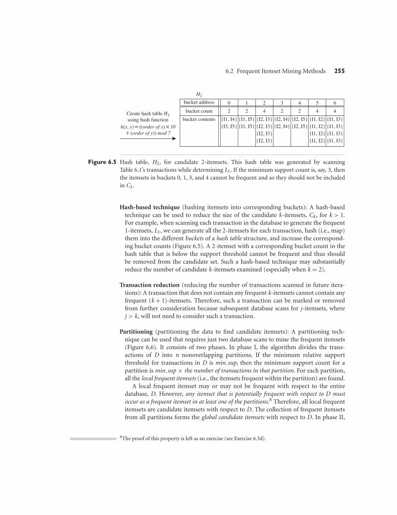
6.2 Frequent Itemset Mining Methods 255
0
2
{I1, I4}{I3, I5}
1
2
{I1, I5}{I1, I5}
2
4
{I2, I3}{I2, I3}{I2, I3}{I2, I3}
3
2
{I2, I4}{I2, I4}
4
2
{I2, I5}{I2, I5}
5
4
{I1, I2}{I1, I2}{I1, I2}{I1, I2}
6
4
{I1, I3}{I1, I3}{I1, I3}{I1, I3}
H2
bucket address
bucket count
bucket contentsCreate hash table H2using hash function
h(x, y)� ((order of x)�10� (order of y)) mod 7
Figure 6.5 Hash table, H2, for candidate 2-itemsets. This hash table was generated by scanningTable 6.1’s transactions while determining L1. If the minimum support count is, say, 3, thenthe itemsets in buckets 0, 1, 3, and 4 cannot be frequent and so they should not be includedin C2.
Hash-based technique (hashing itemsets into corresponding buckets): A hash-basedtechnique can be used to reduce the size of the candidate k-itemsets, Ck , for k > 1.For example, when scanning each transaction in the database to generate the frequent1-itemsets, L1, we can generate all the 2-itemsets for each transaction, hash (i.e., map)them into the different buckets of a hash table structure, and increase the correspond-ing bucket counts (Figure 6.5). A 2-itemset with a corresponding bucket count in thehash table that is below the support threshold cannot be frequent and thus shouldbe removed from the candidate set. Such a hash-based technique may substantiallyreduce the number of candidate k-itemsets examined (especially when k = 2).
Transaction reduction (reducing the number of transactions scanned in future itera-tions): A transaction that does not contain any frequent k-itemsets cannot contain anyfrequent (k + 1)-itemsets. Therefore, such a transaction can be marked or removedfrom further consideration because subsequent database scans for j-itemsets, wherej > k, will not need to consider such a transaction.
Partitioning (partitioning the data to find candidate itemsets): A partitioning tech-nique can be used that requires just two database scans to mine the frequent itemsets(Figure 6.6). It consists of two phases. In phase I, the algorithm divides the trans-actions of D into n nonoverlapping partitions. If the minimum relative supportthreshold for transactions in D is min sup, then the minimum support count for apartition is min sup × the number of transactions in that partition. For each partition,all the local frequent itemsets (i.e., the itemsets frequent within the partition) are found.
A local frequent itemset may or may not be frequent with respect to the entiredatabase, D. However, any itemset that is potentially frequent with respect to D mustoccur as a frequent itemset in at least one of the partitions.8 Therefore, all local frequentitemsets are candidate itemsets with respect to D. The collection of frequent itemsetsfrom all partitions forms the global candidate itemsets with respect to D. In phase II,
8The proof of this property is left as an exercise (see Exercise 6.3d).

256 Chapter 6 Mining Frequent Patterns, Associations, and Correlations
Transactionsin D
Frequentitemsets
in D
Divide D into n
partitions
Find thefrequentitemsets
local to eachpartition(1 scan)
Combineall localfrequentitemsetsto form
candidateitemset
Find globalfrequentitemsetsamong
candidates(1 scan)
Phase I
Phase II
Figure 6.6 Mining by partitioning the data.
a second scan of D is conducted in which the actual support of each candidate isassessed to determine the global frequent itemsets. Partition size and the number ofpartitions are set so that each partition can fit into main memory and therefore beread only once in each phase.
Sampling (mining on a subset of the given data): The basic idea of the samplingapproach is to pick a random sample S of the given data D, and then search forfrequent itemsets in S instead of D. In this way, we trade off some degree of accuracyagainst efficiency. The S sample size is such that the search for frequent itemsets in Scan be done in main memory, and so only one scan of the transactions in S is requiredoverall. Because we are searching for frequent itemsets in S rather than in D, it ispossible that we will miss some of the global frequent itemsets.
To reduce this possibility, we use a lower support threshold than minimum supportto find the frequent itemsets local to S (denoted LS). The rest of the database isthen used to compute the actual frequencies of each itemset in LS. A mechanism isused to determine whether all the global frequent itemsets are included in LS. If LS
actually contains all the frequent itemsets in D, then only one scan of D is required.Otherwise, a second pass can be done to find the frequent itemsets that were missedin the first pass. The sampling approach is especially beneficial when efficiency is ofutmost importance such as in computationally intensive applications that must berun frequently.
Dynamic itemset counting (adding candidate itemsets at different points during ascan): A dynamic itemset counting technique was proposed in which the databaseis partitioned into blocks marked by start points. In this variation, new candidateitemsets can be added at any start point, unlike in Apriori, which determines newcandidate itemsets only immediately before each complete database scan. The tech-nique uses the count-so-far as the lower bound of the actual count. If the count-so-farpasses the minimum support, the itemset is added into the frequent itemset collectionand can be used to generate longer candidates. This leads to fewer database scans thanwith Apriori for finding all the frequent itemsets.
Other variations are discussed in the next chapter.

6.2 Frequent Itemset Mining Methods 257
6.2.4 A Pattern-Growth Approach for MiningFrequent Itemsets
As we have seen, in many cases the Apriori candidate generate-and-test method signifi-cantly reduces the size of candidate sets, leading to good performance gain. However, itcan suffer from two nontrivial costs:
It may still need to generate a huge number of candidate sets. For example, if there are104 frequent 1-itemsets, the Apriori algorithm will need to generate more than 107
candidate 2-itemsets.
It may need to repeatedly scan the whole database and check a large set of candidates bypattern matching. It is costly to go over each transaction in the database to determinethe support of the candidate itemsets.
“Can we design a method that mines the complete set of frequent itemsets without sucha costly candidate generation process?” An interesting method in this attempt is calledfrequent pattern growth, or simply FP-growth, which adopts a divide-and-conquerstrategy as follows. First, it compresses the database representing frequent items into afrequent pattern tree, or FP-tree, which retains the itemset association information. Itthen divides the compressed database into a set of conditional databases (a special kind ofprojected database), each associated with one frequent item or “pattern fragment,” andmines each database separately. For each “pattern fragment,” only its associated data setsneed to be examined. Therefore, this approach may substantially reduce the size of thedata sets to be searched, along with the “growth” of patterns being examined. You willsee how it works in Example 6.5.
Example 6.5 FP-growth (finding frequent itemsets without candidate generation). We reexaminethe mining of transaction database, D, of Table 6.1 in Example 6.3 using the frequentpattern growth approach.
The first scan of the database is the same as Apriori, which derives the set of frequentitems (1-itemsets) and their support counts (frequencies). Let the minimum supportcount be 2. The set of frequent items is sorted in the order of descending support count.This resulting set or list is denoted by L. Thus, we have L = {{I2: 7}, {I1: 6}, {I3: 6},{I4: 2}, {I5: 2}}.
An FP-tree is then constructed as follows. First, create the root of the tree, labeledwith “null.” Scan database D a second time. The items in each transaction are processedin L order (i.e., sorted according to descending support count), and a branch is createdfor each transaction. For example, the scan of the first transaction, “T100: I1, I2, I5,”which contains three items (I2, I1, I5 in L order), leads to the construction of the firstbranch of the tree with three nodes, 〈I2: 1〉, 〈I1: 1〉, and 〈I5: 1〉, where I2 is linked as achild to the root, I1 is linked to I2, and I5 is linked to I1. The second transaction, T200,contains the items I2 and I4 in L order, which would result in a branch where I2 is linkedto the root and I4 is linked to I2. However, this branch would share a common prefix,I2, with the existing path for T100. Therefore, we instead increment the count of the I2node by 1, and create a new node, 〈I4: 1〉, which is linked as a child to 〈I2: 2〉. In general,

258 Chapter 6 Mining Frequent Patterns, Associations, and Correlations
I2I1I3I4I5
76622
I1:2
I3:2I4:1I3:2
I4:1
I5:1
I5:1
I1:4
I2:7
null{}
I3:2
Node-linkItem ID
Supportcount
Figure 6.7 An FP-tree registers compressed, frequent pattern information.
when considering the branch to be added for a transaction, the count of each node alonga common prefix is incremented by 1, and nodes for the items following the prefix arecreated and linked accordingly.
To facilitate tree traversal, an item header table is built so that each item points to itsoccurrences in the tree via a chain of node-links. The tree obtained after scanning allthe transactions is shown in Figure 6.7 with the associated node-links. In this way, theproblem of mining frequent patterns in databases is transformed into that of mining theFP-tree.
The FP-tree is mined as follows. Start from each frequent length-1 pattern (as aninitial suffix pattern), construct its conditional pattern base (a “sub-database,” whichconsists of the set of prefix paths in the FP-tree co-occurring with the suffix pattern),then construct its (conditional) FP-tree, and perform mining recursively on the tree. Thepattern growth is achieved by the concatenation of the suffix pattern with the frequentpatterns generated from a conditional FP-tree.
Mining of the FP-tree is summarized in Table 6.2 and detailed as follows. We firstconsider I5, which is the last item in L, rather than the first. The reason for starting atthe end of the list will become apparent as we explain the FP-tree mining process. I5occurs in two FP-tree branches of Figure 6.7. (The occurrences of I5 can easily be foundby following its chain of node-links.) The paths formed by these branches are 〈I2, I1,I5: 1〉 and 〈I2, I1, I3, I5: 1〉. Therefore, considering I5 as a suffix, its corresponding twoprefix paths are 〈I2, I1: 1〉 and 〈I2, I1, I3: 1〉, which form its conditional pattern base.Using this conditional pattern base as a transaction database, we build an I5-conditionalFP-tree, which contains only a single path, 〈I2: 2, I1: 2〉; I3 is not included because itssupport count of 1 is less than the minimum support count. The single path generatesall the combinations of frequent patterns: {I2, I5: 2}, {I1, I5: 2}, {I2, I1, I5: 2}.
For I4, its two prefix paths form the conditional pattern base, {{I2 I1: 1}, {I2: 1}},which generates a single-node conditional FP-tree, 〈I2: 2〉, and derives one frequentpattern, {I2, I4: 2}.

6.2 Frequent Itemset Mining Methods 259
Table 6.2 Mining the FP-Tree by Creating Conditional (Sub-)Pattern Bases
Item Conditional Pattern Base Conditional FP-tree Frequent Patterns GeneratedI5 {{I2, I1: 1}, {I2, I1, I3: 1}} 〈I2: 2, I1: 2〉 {I2, I5: 2}, {I1, I5: 2}, {I2, I1, I5: 2}I4 {{I2, I1: 1}, {I2: 1}} 〈I2: 2〉 {I2, I4: 2}I3 {{I2, I1: 2}, {I2: 2}, {I1: 2}} 〈I2: 4, I1: 2〉, 〈I1: 2〉 {I2, I3: 4}, {I1, I3: 4}, {I2, I1, I3: 2}I1 {{I2: 4}} 〈I2: 4〉 {I2, I1: 4}
I2 4 I2:4
I1:2
I1:2
Node-linkItem ID
Supportcount null{}
I1 4
Figure 6.8 The conditional FP-tree associated with the conditional node I3.
Similar to the preceding analysis, I3’s conditional pattern base is {{I2, I1: 2}, {I2: 2},{I1: 2}}. Its conditional FP-tree has two branches, 〈I2: 4, I1: 2〉 and 〈I1: 2〉, as shownin Figure 6.8, which generates the set of patterns {{I2, I3: 4}, {I1, I3: 4}, {I2, I1, I3: 2}}.Finally, I1’s conditional pattern base is {{I2: 4}}, with an FP-tree that contains only onenode, 〈I2: 4〉, which generates one frequent pattern, {I2, I1: 4}. This mining process issummarized in Figure 6.9.
The FP-growth method transforms the problem of finding long frequent patternsinto searching for shorter ones in much smaller conditional databases recursively andthen concatenating the suffix. It uses the least frequent items as a suffix, offering goodselectivity. The method substantially reduces the search costs.
When the database is large, it is sometimes unrealistic to construct a main memory-based FP-tree. An interesting alternative is to first partition the database into a setof projected databases, and then construct an FP-tree and mine it in each projecteddatabase. This process can be recursively applied to any projected database if its FP-treestill cannot fit in main memory.
A study of the FP-growth method performance shows that it is efficient and scalablefor mining both long and short frequent patterns, and is about an order of magnitudefaster than the Apriori algorithm.
6.2.5 Mining Frequent Itemsets Using the Vertical Data Format
Both the Apriori and FP-growth methods mine frequent patterns from a set of trans-actions in TID-itemset format (i.e., {TID : itemset}), where TID is a transaction IDand itemset is the set of items bought in transaction TID. This is known as thehorizontal data format. Alternatively, data can be presented in item-TID set format

260 Chapter 6 Mining Frequent Patterns, Associations, and Correlations
Algorithm: FP growth. Mine frequent itemsets using an FP-tree by pattern fragment growth.
Input:
D, a transaction database;
min sup, the minimum support count threshold.
Output: The complete set of frequent patterns.
Method:
1. The FP-tree is constructed in the following steps:
(a) Scan the transaction database D once. Collect F , the set of frequent items, and theirsupport counts. Sort F in support count descending order as L, the list of frequent items.
(b) Create the root of an FP-tree, and label it as “null.” For each transaction Trans in D do thefollowing.Select and sort the frequent items in Trans according to the order of L. Let the sortedfrequent item list in Trans be [p|P], where p is the first element and P is the remaininglist. Call insert tree([p|P], T), which is performed as follows. If T has a child N such thatN.item-name = p.item-name, then increment N ’s count by 1; else create a new node N ,and let its count be 1, its parent link be linked to T , and its node-link to the nodes withthe same item-name via the node-link structure. If P is nonempty, call insert tree(P, N)
recursively.
2. The FP-tree is mined by calling FP growth(FP tree, null), which is implemented as follows.
procedure FP growth(Tree, α)(1) if Tree contains a single path P then(2) for each combination (denoted as β) of the nodes in the path P(3) generate pattern β ∪ α with support count = minimum support count of nodes in β;(4) else for each ai in the header of Tree {(5) generate pattern β = ai ∪ α with support count = ai .support count ;(6) construct β’s conditional pattern base and then β’s conditional FP tree Treeβ ;(7) if Treeβ �= ∅ then(8) call FP growth(Treeβ , β); }
Figure 6.9 FP-growth algorithm for discovering frequent itemsets without candidate generation.
(i.e., {item : TID set}), where item is an item name, and TID set is the set of transactionidentifiers containing the item. This is known as the vertical data format.
In this subsection, we look at how frequent itemsets can also be mined effi-ciently using vertical data format, which is the essence of the Eclat (Equivalence ClassTransformation) algorithm.
Example 6.6 Mining frequent itemsets using the vertical data format. Consider the horizontaldata format of the transaction database, D, of Table 6.1 in Example 6.3. This can betransformed into the vertical data format shown in Table 6.3 by scanning the dataset once.
Mining can be performed on this data set by intersecting the TID sets of every pairof frequent single items. The minimum support count is 2. Because every single item is

6.2 Frequent Itemset Mining Methods 261
Table 6.3 The Vertical Data Format of the Transaction DataSet D of Table 6.1
itemset TID setI1 {T100, T400, T500, T700, T800, T900}I2 {T100, T200, T300, T400, T600, T800, T900}I3 {T300, T500, T600, T700, T800, T900}I4 {T200, T400}I5 {T100, T800}
Table 6.4 2-Itemsets in Vertical Data Format
itemset TID set{I1, I2} {T100, T400, T800, T900}{I1, I3} {T500, T700, T800, T900}{I1, I4} {T400}{I1, I5} {T100, T800}{I2, I3} {T300, T600, T800, T900}{I2, I4} {T200, T400}{I2, I5} {T100, T800}{I3, I5} {T800}
Table 6.5 3-Itemsets in Vertical Data Format
itemset TID set{I1, I2, I3} {T800, T900}{I1, I2, I5} {T100, T800}
frequent in Table 6.3, there are 10 intersections performed in total, which lead to eightnonempty 2-itemsets, as shown in Table 6.4. Notice that because the itemsets {I1, I4}and {I3, I5} each contain only one transaction, they do not belong to the set of frequent2-itemsets.
Based on the Apriori property, a given 3-itemset is a candidate 3-itemset only if everyone of its 2-itemset subsets is frequent. The candidate generation process here will gen-erate only two 3-itemsets: {I1, I2, I3} and {I1, I2, I5}. By intersecting the TID sets of anytwo corresponding 2-itemsets of these candidate 3-itemsets, it derives Table 6.5, wherethere are only two frequent 3-itemsets: {I1, I2, I3: 2} and {I1, I2, I5: 2}.
Example 6.6 illustrates the process of mining frequent itemsets by exploring thevertical data format. First, we transform the horizontally formatted data into thevertical format by scanning the data set once. The support count of an itemset is simplythe length of the TID set of the itemset. Starting with k = 1, the frequent k-itemsetscan be used to construct the candidate (k + 1)-itemsets based on the Apriori property.

262 Chapter 6 Mining Frequent Patterns, Associations, and Correlations
The computation is done by intersection of the TID sets of the frequent k-itemsets tocompute the TID sets of the corresponding (k + 1)-itemsets. This process repeats, withk incremented by 1 each time, until no frequent itemsets or candidate itemsets can befound.
Besides taking advantage of the Apriori property in the generation of candidate(k + 1)-itemset from frequent k-itemsets, another merit of this method is that thereis no need to scan the database to find the support of (k + 1)-itemsets (for k ≥ 1).This is because the TID set of each k-itemset carries the complete information requiredfor counting such support. However, the TID sets can be quite long, taking substantialmemory space as well as computation time for intersecting the long sets.
To further reduce the cost of registering long TID sets, as well as the subsequentcosts of intersections, we can use a technique called diffset, which keeps track of onlythe differences of the TID sets of a (k + 1)-itemset and a corresponding k-itemset. Forinstance, in Example 6.6 we have {I1} = {T100, T400, T500, T700, T800, T900} and {I1,I2} = {T100, T400, T800, T900}. The diffset between the two is diffset({I1, I2}, {I1}) ={T500, T700}. Thus, rather than recording the four TIDs that make up the intersection of{I1} and {I2}, we can instead use diffset to record just two TIDs, indicating the differencebetween {I1} and {I1, I2}. Experiments show that in certain situations, such as when thedata set contains many dense and long patterns, this technique can substantially reducethe total cost of vertical format mining of frequent itemsets.
6.2.6 Mining Closed and Max Patterns
In Section 6.1.2 we saw how frequent itemset mining may generate a huge number offrequent itemsets, especially when the min sup threshold is set low or when there existlong patterns in the data set. Example 6.2 showed that closed frequent itemsets9 cansubstantially reduce the number of patterns generated in frequent itemset mining whilepreserving the complete information regarding the set of frequent itemsets. That is, fromthe set of closed frequent itemsets, we can easily derive the set of frequent itemsets andtheir support. Thus, in practice, it is more desirable to mine the set of closed frequentitemsets rather than the set of all frequent itemsets in most cases.
“How can we mine closed frequent itemsets?” A naïve approach would be to first minethe complete set of frequent itemsets and then remove every frequent itemset that is aproper subset of, and carries the same support as, an existing frequent itemset. However,this is quite costly. As shown in Example 6.2, this method would have to first derive2100 − 1 frequent itemsets to obtain a length-100 frequent itemset, all before it couldbegin to eliminate redundant itemsets. This is prohibitively expensive. In fact, there existonly a very small number of closed frequent itemsets in Example 6.2’s data set.
A recommended methodology is to search for closed frequent itemsets directly dur-ing the mining process. This requires us to prune the search space as soon as we
9Remember that X is a closed frequent itemset in a data set S if there exists no proper super-itemset Ysuch that Y has the same support count as X in S, and X satisfies minimum support.

6.2 Frequent Itemset Mining Methods 263
can identify the case of closed itemsets during mining. Pruning strategies include thefollowing:
Item merging: If every transaction containing a frequent itemset X also contains an itemsetY but not any proper superset of Y , then X ∪ Y forms a frequent closed itemset and thereis no need to search for any itemset containing X but no Y .
For example, in Table 6.2 of Example 6.5, the projected conditional database forprefix itemset {I5:2} is {{I2, I1}, {I2, I1, I3}}, from which we can see that each of itstransactions contains itemset {I2, I1} but no proper superset of {I2, I1}. Itemset {I2,I1} can be merged with {I5} to form the closed itemset, {I5, I2, I1: 2}, and we do notneed to mine for closed itemsets that contain I5 but not {I2, I1}.
Sub-itemset pruning: If a frequent itemset X is a proper subset of an already found fre-quent closed itemset Y and support count(X)=support count(Y), then X and all of X’sdescendants in the set enumeration tree cannot be frequent closed itemsets and thus canbe pruned.
Similar to Example 6.2, suppose a transaction database has only two trans-actions: {〈a1, a2, . . . , a100〉, 〈a1, a2, . . . , a50〉}, and the minimum support count ismin sup = 2. The projection on the first item, a1, derives the frequent itemset, {a1,a2, . . . , a50 : 2}, based on the itemset merging optimization. Because support({a2}) =support({a1, a2, . . . , a50}) = 2, and {a2} is a proper subset of {a1, a2, . . . , a50}, thereis no need to examine a2 and its projected database. Similar pruning can be donefor a3, . . . , a50 as well. Thus, the mining of closed frequent itemsets in this data setterminates after mining a1’s projected database.
Item skipping: In the depth-first mining of closed itemsets, at each level, there will bea prefix itemset X associated with a header table and a projected database. If a localfrequent item p has the same support in several header tables at different levels, we cansafely prune p from the header tables at higher levels.
Consider, for example, the previous transaction database having only two trans-actions: {〈a1, a2, . . . , a100〉, 〈a1, a2, . . . , a50〉}, where min sup = 2. Because a2 in a1’sprojected database has the same support as a2 in the global header table, a2 can bepruned from the global header table. Similar pruning can be done for a3, . . . , a50.There is no need to mine anything more after mining a1’s projected database.
Besides pruning the search space in the closed itemset mining process, anotherimportant optimization is to perform efficient checking of each newly derived frequentitemset to see whether it is closed. This is because the mining process cannot ensure thatevery generated frequent itemset is closed.
When a new frequent itemset is derived, it is necessary to perform two kinds ofclosure checking: (1) superset checking, which checks if this new frequent itemset is asuperset of some already found closed itemsets with the same support, and (2) subsetchecking, which checks whether the newly found itemset is a subset of an already foundclosed itemset with the same support.
If we adopt the item merging pruning method under a divide-and-conquer frame-work, then the superset checking is actually built-in and there is no need to explicitly

264 Chapter 6 Mining Frequent Patterns, Associations, and Correlations
perform superset checking. This is because if a frequent itemset X ∪ Y is found laterthan itemset X , and carries the same support as X , it must be in X ’s projected databaseand must have been generated during itemset merging.
To assist in subset checking, a compressed pattern-tree can be constructed to main-tain the set of closed itemsets mined so far. The pattern-tree is similar in structure to theFP-tree except that all the closed itemsets found are stored explicitly in the correspond-ing tree branches. For efficient subset checking, we can use the following property: If thecurrent itemset Sc can be subsumed by another already found closed itemset Sa, then (1) Sc
and Sa have the same support, (2) the length of Sc is smaller than that of Sa, and (3) all ofthe items in Sc are contained in Sa.
Based on this property, a two-level hash index structure can be built for fast access-ing of the pattern-tree: The first level uses the identifier of the last item in Sc as a hash key(since this identifier must be within the branch of Sc), and the second level uses the sup-port of Sc as a hash key (since Sc and Sa have the same support). This will substantiallyspeed up the subset checking process.
This discussion illustrates methods for efficient mining of closed frequent itemsets.“Can we extend these methods for efficient mining of maximal frequent itemsets?” Becausemaximal frequent itemsets share many similarities with closed frequent itemsets, manyof the optimization techniques developed here can be extended to mining maximalfrequent itemsets. However, we leave this method as an exercise for interested readers.
6.3 Which Patterns Are Interesting?—PatternEvaluation Methods
Most association rule mining algorithms employ a support–confidence framework.Although minimum support and confidence thresholds help weed out or exclude theexploration of a good number of uninteresting rules, many of the rules generated arestill not interesting to the users. Unfortunately, this is especially true when mining atlow support thresholds or mining for long patterns. This has been a major bottleneck forsuccessful application of association rule mining.
In this section, we first look at how even strong association rules can be uninterestingand misleading (Section 6.3.1). We then discuss how the support–confidence frame-work can be supplemented with additional interestingness measures based on correlationanalysis (Section 6.3.2). Section 6.3.3 presents additional pattern evaluation measures.It then provides an overall comparison of all the measures discussed here. By the end,you will learn which pattern evaluation measures are most effective for the discovery ofonly interesting rules.
6.3.1 Strong Rules Are Not Necessarily Interesting
Whether or not a rule is interesting can be assessed either subjectively or objectively.Ultimately, only the user can judge if a given rule is interesting, and this judgment, being

6.3 Which Patterns Are Interesting?—Pattern Evaluation Methods 265
subjective, may differ from one user to another. However, objective interestingness mea-sures, based on the statistics “behind” the data, can be used as one step toward the goalof weeding out uninteresting rules that would otherwise be presented to the user.
“How can we tell which strong association rules are really interesting?” Let’s examinethe following example.
Example 6.7 A misleading “strong” association rule. Suppose we are interested in analyzing trans-actions at AllElectronics with respect to the purchase of computer games and videos.Let game refer to the transactions containing computer games, and video refer to thosecontaining videos. Of the 10,000 transactions analyzed, the data show that 6000 of thecustomer transactions included computer games, while 7500 included videos, and 4000included both computer games and videos. Suppose that a data mining program fordiscovering association rules is run on the data, using a minimum support of, say, 30%and a minimum confidence of 60%. The following association rule is discovered:
buys(X , “computer games”) ⇒ buys(X , “videos”)
[support = 40%, confidence = 66%]. (6.6)
Rule (6.6) is a strong association rule and would therefore be reported, since its supportvalue of 4000
10,000 = 40% and confidence value of 40006000 = 66% satisfy the minimum support
and minimum confidence thresholds, respectively. However, Rule (6.6) is misleadingbecause the probability of purchasing videos is 75%, which is even larger than 66%. Infact, computer games and videos are negatively associated because the purchase of oneof these items actually decreases the likelihood of purchasing the other. Without fullyunderstanding this phenomenon, we could easily make unwise business decisions basedon Rule (6.6).
Example 6.7 also illustrates that the confidence of a rule A ⇒ B can be deceiving. Itdoes not measure the real strength (or lack of strength) of the correlation and implica-tion between A and B. Hence, alternatives to the support–confidence framework can beuseful in mining interesting data relationships.
6.3.2 From Association Analysis to Correlation Analysis
As we have seen so far, the support and confidence measures are insufficient at filteringout uninteresting association rules. To tackle this weakness, a correlation measure canbe used to augment the support–confidence framework for association rules. This leadsto correlation rules of the form
A ⇒ B [support, confidence, correlation]. (6.7)
That is, a correlation rule is measured not only by its support and confidence but alsoby the correlation between itemsets A and B. There are many different correlation mea-sures from which to choose. In this subsection, we study several correlation measures todetermine which would be good for mining large data sets.

266 Chapter 6 Mining Frequent Patterns, Associations, and Correlations
Lift is a simple correlation measure that is given as follows. The occurrence of itemsetA is independent of the occurrence of itemset B if P(A ∪ B) = P(A)P(B); otherwise,itemsets A and B are dependent and correlated as events. This definition can easily beextended to more than two itemsets. The lift between the occurrence of A and B can bemeasured by computing
lift(A, B) = P(A ∪ B)
P(A)P(B). (6.8)
If the resulting value of Eq. (6.8) is less than 1, then the occurrence of A is negativelycorrelated with the occurrence of B, meaning that the occurrence of one likely leads tothe absence of the other one. If the resulting value is greater than 1, then A and B arepositively correlated, meaning that the occurrence of one implies the occurrence of theother. If the resulting value is equal to 1, then A and B are independent and there is nocorrelation between them.
Equation (6.8) is equivalent to P(B|A)/P(B), or conf(A ⇒ B)/sup(B), which is alsoreferred to as the lift of the association (or correlation) rule A ⇒ B. In other words, itassesses the degree to which the occurrence of one “lifts” the occurrence of the other. Forexample, if A corresponds to the sale of computer games and B corresponds to the saleof videos, then given the current market conditions, the sale of games is said to increaseor “lift” the likelihood of the sale of videos by a factor of the value returned by Eq. (6.8).
Let’s go back to the computer game and video data of Example 6.7.
Example 6.8 Correlation analysis using lift. To help filter out misleading “strong” associations ofthe form A ⇒ B from the data of Example 6.7, we need to study how the two item-sets, A and B, are correlated. Let game refer to the transactions of Example 6.7 that donot contain computer games, and video refer to those that do not contain videos. Thetransactions can be summarized in a contingency table, as shown in Table 6.6.
From the table, we can see that the probability of purchasing a computer gameis P({game}) = 0.60, the probability of purchasing a video is P({video}) = 0.75, andthe probability of purchasing both is P({game,video}) = 0.40. By Eq. (6.8), the lift ofRule (6.6) is P({game, video})/(P({game}) × P({video})) = 0.40/(0.60 × 0.75) = 0.89.Because this value is less than 1, there is a negative correlation between the occur-rence of {game} and {video}. The numerator is the likelihood of a customer purchasingboth, while the denominator is what the likelihood would have been if the two pur-chases were completely independent. Such a negative correlation cannot be identifiedby a support–confidence framework.
The second correlation measure that we study is the χ2 measure, which was intro-duced in Chapter 3 (Eq. 3.1). To compute the χ2 value, we take the squared differencebetween the observed and expected value for a slot (A and B pair) in the contin-gency table, divided by the expected value. This amount is summed for all slots of thecontingency table. Let’s perform a χ2 analysis of Example 6.8.

6.3 Which Patterns Are Interesting?—Pattern Evaluation Methods 267
Table 6.6 2 × 2 Contingency Table Summarizing theTransactions with Respect to Game andVideo Purchases
game game �row
video 4000 3500 7500
video 2000 500 2500
�col 6000 4000 10,000
Table 6.7 Table 6.6 Contingency Table, Now withthe Expected Values
game game �row
video 4000 (4500) 3500 (3000) 7500
video 2000 (1500) 500 (1000) 2500
�col 6000 4000 10,000
Example 6.9 Correlation analysis using χ2. To compute the correlation using χ2 analysis for nom-inal data, we need the observed value and expected value (displayed in parenthesis) foreach slot of the contingency table, as shown in Table 6.7. From the table, we can computethe χ2 value as follows:
χ2 = �(observed − expected)2
expected= (4000 − 4500)2
4500+ (3500 − 3000)2
3000
+ (2000 − 1500)2
1500+ (500 − 1000)2
1000= 555.6.
Because the χ2 value is greater than 1, and the observed value of the slot (game, video) =4000, which is less than the expected value of 4500, buying game and buying video arenegatively correlated. This is consistent with the conclusion derived from the analysis ofthe lift measure in Example 6.8.
6.3.3 A Comparison of Pattern Evaluation Measures
The above discussion shows that instead of using the simple support–confidence frame-work to evaluate frequent patterns, other measures, such as lift and χ2, often disclosemore intrinsic pattern relationships. How effective are these measures? Should we alsoconsider other alternatives?
Researchers have studied many pattern evaluation measures even before the start ofin-depth research on scalable methods for mining frequent patterns. Recently, severalother pattern evaluation measures have attracted interest. In this subsection, we present

268 Chapter 6 Mining Frequent Patterns, Associations, and Correlations
four such measures: all confidence, max confidence, Kulczynski, and cosine. We’ll thencompare their effectiveness with respect to one another and with respect to the lift andχ2 measures.
Given two itemsets, A and B, the all confidence measure of A and B is defined as
all conf(A,B) = sup(A ∪ B)
max{sup(A), sup(B)} = min {P(A|B),P(B|A)}, (6.9)
where max{sup(A), sup(B)} is the maximum support of the itemsets A and B. Thus,all conf(A,B) is also the minimum confidence of the two association rules related toA and B, namely, “A ⇒ B” and “B ⇒ A.”
Given two itemsets, A and B, the max confidence measure of A and B is defined as
max conf(A, B) = max{P(A |B),P(B |A)}. (6.10)
The max conf measure is the maximum confidence of the two association rules,“A ⇒ B” and “B ⇒ A.”
Given two itemsets, A and B, the Kulczynski measure of A and B (abbreviated asKulc) is defined as
Kulc(A, B) = 1
2(P(A|B) + P(B|A)). (6.11)
It was proposed in 1927 by Polish mathematician S. Kulczynski. It can be viewed as anaverage of two confidence measures. That is, it is the average of two conditional prob-abilities: the probability of itemset B given itemset A, and the probability of itemset Agiven itemset B.
Finally, given two itemsets, A and B, the cosine measure of A and B is defined as
cosine(A, B) = P(A ∪ B)√P(A) × P(B)
= sup(A ∪ B)√sup(A) × sup(B)
=√
P(A|B) × P(B|A). (6.12)
The cosine measure can be viewed as a harmonized lift measure: The two formulae aresimilar except that for cosine, the square root is taken on the product of the probabilitiesof A and B. This is an important difference, however, because by taking the square root,the cosine value is only influenced by the supports of A, B, and A ∪ B, and not by thetotal number of transactions.
Each of these four measures defined has the following property: Its value is onlyinfluenced by the supports of A, B, and A ∪ B, or more exactly, by the conditional prob-abilities of P(A|B) and P(B|A), but not by the total number of transactions. Anothercommon property is that each measure ranges from 0 to 1, and the higher the value, thecloser the relationship between A and B.
Now, together with lift and χ2, we have introduced in total six pattern evaluationmeasures. You may wonder, “Which is the best in assessing the discovered pattern rela-tionships?” To answer this question, we examine their performance on some typicaldata sets.

6.3 Which Patterns Are Interesting?—Pattern Evaluation Methods 269
Table 6.8 2 × 2 Contingency Table for Two Items
milk milk �row
coffee mc mc c
coffee mc mc c
�col m m �
Table 6.9 Comparison of Six Pattern Evaluation Measures Using Contingency Tablesfor a Variety of Data Sets
DataSet mc mc mc mc χ2 lift all conf. max conf. Kulc. cosineD1 10,000 1000 1000 100,000 90557 9.26 0.91 0.91 0.91 0.91
D2 10,000 1000 1000 100 0 1 0.91 0.91 0.91 0.91
D3 100 1000 1000 100,000 670 8.44 0.09 0.09 0.09 0.09
D4 1000 1000 1000 100,000 24740 25.75 0.5 0.5 0.5 0.5
D5 1000 100 10,000 100,000 8173 9.18 0.09 0.91 0.5 0.29
D6 1000 10 100,000 100,000 965 1.97 0.01 0.99 0.5 0.10
Example 6.10 Comparison of six pattern evaluation measures on typical data sets. The relationshipsbetween the purchases of two items, milk and coffee, can be examined by summarizingtheir purchase history in Table 6.8, a 2 × 2 contingency table, where an entry such as mcrepresents the number of transactions containing both milk and coffee.
Table 6.9 shows a set of transactional data sets with their corresponding contin-gency tables and the associated values for each of the six evaluation measures. Let’sfirst examine the first four data sets, D1 through D4. From the table, we see that mand c are positively associated in D1 and D2, negatively associated in D3, and neu-tral in D4. For D1 and D2, m and c are positively associated because mc (10,000)is considerably greater than mc (1000) and mc (1000). Intuitively, for people whobought milk (m = 10,000 + 1000 = 11,000), it is very likely that they also bought coffee(mc/m = 10/11 = 91%), and vice versa.
The results of the four newly introduced measures show that m and c are stronglypositively associated in both data sets by producing a measure value of 0.91. However,lift and χ2 generate dramatically different measure values for D1 and D2 due to theirsensitivity to mc. In fact, in many real-world scenarios, mc is usually huge and unstable.For example, in a market basket database, the total number of transactions could fluctu-ate on a daily basis and overwhelmingly exceed the number of transactions containingany particular itemset. Therefore, a good interestingness measure should not be affectedby transactions that do not contain the itemsets of interest; otherwise, it would generateunstable results, as illustrated in D1 and D2.

270 Chapter 6 Mining Frequent Patterns, Associations, and Correlations
Similarly, in D3, the four new measures correctly show that m and c are stronglynegatively associated because the m to c ratio equals the mc to m ratio, that is,100/1100 = 9.1%. However, lift and χ2 both contradict this in an incorrect way: Theirvalues for D2 are between those for D1 and D3.
For data set D4, both lift and χ2 indicate a highly positive association betweenm and c, whereas the others indicate a “neutral” association because the ratio of mc tomc equals the ratio of mc to mc, which is 1. This means that if a customer buyscoffee (or milk), the probability that he or she will also purchase milk (or coffee) isexactly 50%.
“Why are lift and χ2 so poor at distinguishing pattern association relationships inthe previous transactional data sets?” To answer this, we have to consider the null-transactions. A null-transaction is a transaction that does not contain any of the item-sets being examined. In our example, mc represents the number of null-transactions.Lift and χ2 have difficulty distinguishing interesting pattern association relationshipsbecause they are both strongly influenced by mc. Typically, the number of null-transactions can outweigh the number of individual purchases because, for example,many people may buy neither milk nor coffee. On the other hand, the other fourmeasures are good indicators of interesting pattern associations because their defi-nitions remove the influence of mc (i.e., they are not influenced by the number ofnull-transactions).
This discussion shows that it is highly desirable to have a measure that has a valuethat is independent of the number of null-transactions. A measure is null-invariant ifits value is free from the influence of null-transactions. Null-invariance is an impor-tant property for measuring association patterns in large transaction databases. Amongthe six discussed measures in this subsection, only lift and χ2 are not null-invariantmeasures.
“Among the all confidence, max confidence, Kulczynski, and cosine measures, whichis best at indicating interesting pattern relationships?”
To answer this question, we introduce the imbalance ratio (IR), which assesses theimbalance of two itemsets, A and B, in rule implications. It is defined as
IR(A,B) = |sup(A) − sup(B)|sup(A) + sup(B) − sup(A ∪ B)
, (6.13)
where the numerator is the absolute value of the difference between the support of theitemsets A and B, and the denominator is the number of transactions containing A orB. If the two directional implications between A and B are the same, then IR(A,B) willbe zero. Otherwise, the larger the difference between the two, the larger the imbalanceratio. This ratio is independent of the number of null-transactions and independent ofthe total number of transactions.
Let’s continue examining the remaining data sets in Example 6.10.
Example 6.11 Comparing null-invariant measures in pattern evaluation. Although the four mea-sures introduced in this section are null-invariant, they may present dramatically

6.4 Summary 271
different values on some subtly different data sets. Let’s examine data sets D5 and D6,shown earlier in Table 6.9, where the two events m and c have unbalanced conditionalprobabilities. That is, the ratio of mc to c is greater than 0.9. This means that knowingthat c occurs should strongly suggest that m occurs also. The ratio of mc to m is less than0.1, indicating that m implies that c is quite unlikely to occur. The all confidence andcosine measures view both cases as negatively associated and the Kulc measure viewsboth as neutral. The max confidence measure claims strong positive associations forthese cases. The measures give very diverse results!
“Which measure intuitively reflects the true relationship between the purchase of milkand coffee?” Due to the “balanced” skewness of the data, it is difficult to argue whetherthe two data sets have positive or negative association. From one point of view, onlymc/(mc + mc) = 1000/(1000 + 10,000) = 9.09% of milk-related transactions containcoffee in D5 and this percentage is 1000/(1000 + 100,000) = 0.99% in D6, both indi-cating a negative association. On the other hand, 90.9% of transactions in D5 (i.e.,mc/(mc + mc) = 1000/(1000 + 100)) and 9% in D6 (i.e., 1000/(1000 + 10)) contain-ing coffee contain milk as well, which indicates a positive association between milk andcoffee. These draw very different conclusions.
For such “balanced” skewness, it could be fair to treat it as neutral, as Kulc does,and in the meantime indicate its skewness using the imbalance ratio (IR). According toEq. (6.13), for D4 we have IR(m, c) = 0, a perfectly balanced case; for D5, IR(m, c) =0.89, a rather imbalanced case; whereas for D6, IR(m, c) = 0.99, a very skewed case.Therefore, the two measures, Kulc and IR, work together, presenting a clear picture forall three data sets, D4 through D6.
In summary, the use of only support and confidence measures to mine associa-tions may generate a large number of rules, many of which can be uninteresting tousers. Instead, we can augment the support–confidence framework with a pattern inter-estingness measure, which helps focus the mining toward rules with strong patternrelationships. The added measure substantially reduces the number of rules gener-ated and leads to the discovery of more meaningful rules. Besides those introduced inthis section, many other interestingness measures have been studied in the literature.Unfortunately, most of them do not have the null-invariance property. Because largedata sets typically have many null-transactions, it is important to consider the null-invariance property when selecting appropriate interestingness measures for patternevaluation. Among the four null-invariant measures studied here, namely all confidence,max confidence, Kulc, and cosine, we recommend using Kulc in conjunction with theimbalance ratio.
6.4 Summary
The discovery of frequent patterns, associations, and correlation relationships amonghuge amounts of data is useful in selective marketing, decision analysis, and businessmanagement. A popular area of application is market basket analysis, which studies

272 Chapter 6 Mining Frequent Patterns, Associations, and Correlations
customers’ buying habits by searching for itemsets that are frequently purchasedtogether (or in sequence).
Association rule mining consists of first finding frequent itemsets (sets of items,such as A and B, satisfying a minimum support threshold, or percentage of the task-relevant tuples), from which strong association rules in the form of A ⇒ B aregenerated. These rules also satisfy a minimum confidence threshold (a prespecifiedprobability of satisfying B under the condition that A is satisfied). Associations can befurther analyzed to uncover correlation rules, which convey statistical correlationsbetween itemsets A and B.
Many efficient and scalable algorithms have been developed for frequent itemsetmining, from which association and correlation rules can be derived. These algo-rithms can be classified into three categories: (1) Apriori-like algorithms, (2) frequentpattern growth–based algorithms such as FP-growth, and (3) algorithms that use thevertical data format.
The Apriori algorithm is a seminal algorithm for mining frequent itemsets forBoolean association rules. It explores the level-wise mining Apriori property that allnonempty subsets of a frequent itemset must also be frequent. At the kth iteration (fork ≥ 2), it forms frequent k-itemset candidates based on the frequent (k − 1)-itemsets,and scans the database once to find the complete set of frequent k-itemsets, Lk .
Variations involving hashing and transaction reduction can be used to make theprocedure more efficient. Other variations include partitioning the data (mining oneach partition and then combining the results) and sampling the data (mining ona data subset). These variations can reduce the number of data scans required to aslittle as two or even one.
Frequent pattern growth is a method of mining frequent itemsets without candidategeneration. It constructs a highly compact data structure (an FP-tree) to compress theoriginal transaction database. Rather than employing the generate-and-test strategy ofApriori-like methods, it focuses on frequent pattern (fragment) growth, which avoidscostly candidate generation, resulting in greater efficiency.
Mining frequent itemsets using the vertical data format (Eclat) is a method thattransforms a given data set of transactions in the horizontal data format of TID-itemset into the vertical data format of item-TID set. It mines the transformeddata set by TID set intersections based on the Apriori property and additionaloptimization techniques such as diffset.
Not all strong association rules are interesting. Therefore, the support–confidenceframework should be augmented with a pattern evaluation measure, which promotesthe mining of interesting rules. A measure is null-invariant if its value is free fromthe influence of null-transactions (i.e., the transactions that do not contain any ofthe itemsets being examined). Among many pattern evaluation measures, we exam-ined lift, χ2, all confidence, max confidence, Kulczynski, and cosine, and showed

6.5 Exercises 273
that only the latter four are null-invariant. We suggest using the Kulczynski measure,together with the imbalance ratio, to present pattern relationships among itemsets.
6.5 Exercises
6.1 Suppose you have the set C of all frequent closed itemsets on a data set D, as wellas the support count for each frequent closed itemset. Describe an algorithm todetermine whether a given itemset X is frequent or not, and the support of X if itis frequent.
6.2 An itemset X is called a generator on a data set D if there does not exist a propersub-itemset Y ⊂ X such that support(X) = support(Y ). A generator X is a frequentgenerator if support(X) passes the minimum support threshold. Let G be the set ofall frequent generators on a data set D.
(a) Can you determine whether an itemset A is frequent and the support of A, if itis frequent, using only G and the support counts of all frequent generators? Ifyes, present your algorithm. Otherwise, what other information is needed? Canyou give an algorithm assuming the information needed is available?
(b) What is the relationship between closed itemsets and generators?
6.3 The Apriori algorithm makes use of prior knowledge of subset support properties.
(a) Prove that all nonempty subsets of a frequent itemset must also be frequent.
(b) Prove that the support of any nonempty subset s′ of itemset s must be at leastas great as the support of s.
(c) Given frequent itemset l and subset s of l, prove that the confidence of the rule“s′ ⇒ (l − s′)” cannot be more than the confidence of “s ⇒ (l − s),” where s′ isa subset of s.
(d) A partitioning variation of Apriori subdivides the transactions of a database Dinto n nonoverlapping partitions. Prove that any itemset that is frequent in Dmust be frequent in at least one partition of D.
6.4 Let c be a candidate itemset in Ck generated by the Apriori algorithm. How manylength-(k − 1) subsets do we need to check in the prune step? Per your previ-ous answer, can you give an improved version of procedure has infrequent subsetin Figure 6.4?
6.5 Section 6.2.2 describes a method for generating association rules from frequentitemsets. Propose a more efficient method. Explain why it is more efficient thanthe one proposed there. (Hint: Consider incorporating the properties of Exercises6.3(b), (c) into your design.)
6.6 A database has five transactions. Let min sup = 60% and min conf = 80%.

274 Chapter 6 Mining Frequent Patterns, Associations, and Correlations
TID items bought
T100 {M, O, N, K, E, Y}T200 {D, O, N, K, E, Y }T300 {M, A, K, E}T400 {M, U, C, K, Y}T500 {C, O, O, K, I, E}
(a) Find all frequent itemsets using Apriori and FP-growth, respectively. Comparethe efficiency of the two mining processes.
(b) List all the strong association rules (with support s and confidence c) matchingthe following metarule, where X is a variable representing customers, and itemi
denotes variables representing items (e.g., “A,” “B,”):
∀x ∈ transaction, buys(X , item1) ∧ buys(X , item2) ⇒ buys(X , item3) [s, c]
6.7 (Implementation project) Using a programming language that you are familiarwith, such as C++ or Java, implement three frequent itemset mining algorithmsintroduced in this chapter: (1) Apriori [AS94b], (2) FP-growth [HPY00], and(3) Eclat [Zak00] (mining using the vertical data format). Compare the perfor-mance of each algorithm with various kinds of large data sets. Write a report toanalyze the situations (e.g., data size, data distribution, minimal support thresh-old setting, and pattern density) where one algorithm may perform better than theothers, and state why.
6.8 A database has four transactions. Let min sup = 60% and min conf = 80%.
cust ID TID items bought (in the form of brand-item category)
01 T100 {King’s-Crab, Sunset-Milk, Dairyland-Cheese, Best-Bread}02 T200 {Best-Cheese, Dairyland-Milk, Goldenfarm-Apple, Tasty-Pie, Wonder-Bread}01 T300 {Westcoast-Apple, Dairyland-Milk, Wonder-Bread, Tasty-Pie}03 T400 {Wonder-Bread, Sunset-Milk, Dairyland-Cheese}
(a) At the granularity of item category (e.g., itemi could be “Milk”), for the ruletemplate,
∀X ∈ transaction, buys(X , item1) ∧ buys(X , item2) ⇒ buys(X , item3) [s, c],
list the frequent k-itemset for the largest k, and all the strong association rules(with their support s and confidence c) containing the frequent k-itemset for thelargest k.
(b) At the granularity of brand-item category (e.g., itemi could be “Sunset-Milk”),for the rule template,
∀X ∈ customer, buys(X , item1) ∧ buys(X , item2) ⇒ buys(X , item3),
list the frequent k-itemset for the largest k (but do not print any rules).

6.5 Exercises 275
6.9 Suppose that a large store has a transactional database that is distributed amongfour locations. Transactions in each component database have the same for-mat, namely Tj : {i1, . . . , im}, where Tj is a transaction identifier, and ik (1 ≤k ≤ m) is the identifier of an item purchased in the transaction. Propose anefficient algorithm to mine global association rules. You may present your algo-rithm in the form of an outline. Your algorithm should not require shippingall the data to one site and should not cause excessive network communicationoverhead.
6.10 Suppose that frequent itemsets are saved for a large transactional database, DB.Discuss how to efficiently mine the (global) association rules under the sameminimum support threshold, if a set of new transactions, denoted as �DB, is(incrementally) added in?
6.11 Most frequent pattern mining algorithms consider only distinct items in a transac-tion. However, multiple occurrences of an item in the same shopping basket, suchas four cakes and three jugs of milk, can be important in transactional data analysis.How can one mine frequent itemsets efficiently considering multiple occurrencesof items? Propose modifications to the well-known algorithms, such as Apriori andFP-growth, to adapt to such a situation.
6.12 (Implementation project) Many techniques have been proposed to furtherimprove the performance of frequent itemset mining algorithms. Taking FP-tree–based frequent pattern growth algorithms (e.g., FP-growth) as an example, imple-ment one of the following optimization techniques. Compare the performance ofyour new implementation with the unoptimized version.
(a) The frequent pattern mining method of Section 6.2.4 uses an FP-tree to gen-erate conditional pattern bases using a bottom-up projection technique (i.e.,project onto the prefix path of an item p). However, one can develop a top-down projection technique, that is, project onto the suffix path of an item p inthe generation of a conditional pattern base. Design and implement such a top-down FP-tree mining method. Compare its performance with the bottom-upprojection method.
(b) Nodes and pointers are used uniformly in an FP-tree in the FP-growth algo-rithm design. However, such a structure may consume a lot of space whenthe data are sparse. One possible alternative design is to explore array- andpointer-based hybrid implementation, where a node may store multiple itemswhen it contains no splitting point to multiple sub-branches. Develop such animplementation and compare it with the original one.
(c) It is time and space consuming to generate numerous conditional pattern basesduring pattern-growth mining. An interesting alternative is to push right thebranches that have been mined for a particular item p, that is, to push them tothe remaining branch(es) of the FP-tree. This is done so that fewer conditionalpattern bases have to be generated and additional sharing can be explored whenmining the remaining FP-tree branches. Design and implement such a methodand conduct a performance study on it.

276 Chapter 6 Mining Frequent Patterns, Associations, and Correlations
6.13 Give a short example to show that items in a strong association rule actually maybe negatively correlated.
6.14 The following contingency table summarizes supermarket transaction data, wherehot dogs refers to the transactions containing hot dogs, hot dogs refers to thetransactions that do not contain hot dogs, hamburgers refers to the transactionscontaining hamburgers, and hamburgers refers to the transactions that do notcontain hamburgers.
hot dogs hot dogs �row
hamburgers 2000 500 2500
hamburgers 1000 1500 2500
�col 3000 2000 5000
(a) Suppose that the association rule “hot dogs ⇒ hamburgers” is mined. Given aminimum support threshold of 25% and a minimum confidence threshold of50%, is this association rule strong?
(b) Based on the given data, is the purchase of hot dogs independent of the purchaseof hamburgers? If not, what kind of correlation relationship exists between thetwo?
(c) Compare the use of the all confidence, max confidence, Kulczynski, and cosinemeasures with lift and correlation on the given data.
6.15 (Implementation project) The DBLP data set (www.informatik.uni-trier.de/∼ley/db/) consists of over one million entries of research papers pub-lished in computer science conferences and journals. Among these entries, thereare a good number of authors that have coauthor relationships.
(a) Propose a method to efficiently mine a set of coauthor relationships that areclosely correlated (e.g., often coauthoring papers together).
(b) Based on the mining results and the pattern evaluation measures discussed inthis chapter, discuss which measure may convincingly uncover close collabora-tion patterns better than others.
(c) Based on the study in (a), develop a method that can roughly predict advi-sor and advisee relationships and the approximate period for such advisorysupervision.
6.6 Bibliographic Notes
Association rule mining was first proposed by Agrawal, Imielinski, and Swami [AIS93].The Apriori algorithm discussed in Section 6.2.1 for frequent itemset mining was pre-sented in Agrawal and Srikant [AS94b]. A variation of the algorithm using a similarpruning heuristic was developed independently by Mannila, Tiovonen, and Verkamo

6.6 Bibliographic Notes 277
[MTV94]. A joint publication combining these works later appeared in Agrawal,Mannila, Srikant et al. [AMS+96]. A method for generating association rules fromfrequent itemsets is described in Agrawal and Srikant [AS94a].
References for the variations of Apriori described in Section 6.2.3 include thefollowing. The use of hash tables to improve association mining efficiency was stud-ied by Park, Chen, and Yu [PCY95a]. The partitioning technique was proposed bySavasere, Omiecinski, and Navathe [SON95]. The sampling approach is discussed inToivonen [Toi96]. A dynamic itemset counting approach is given in Brin, Motwani,Ullman, and Tsur [BMUT97]. An efficient incremental updating of mined associationrules was proposed by Cheung, Han, Ng, and Wong [CHNW96]. Parallel and dis-tributed association data mining under the Apriori framework was studied by Park,Chen, and Yu [PCY95b]; Agrawal and Shafer [AS96]; and Cheung, Han, Ng, et al.[CHN+96]. Another parallel association mining method, which explores itemset clus-tering using a vertical database layout, was proposed in Zaki, Parthasarathy, Ogihara,and Li [ZPOL97].
Other scalable frequent itemset mining methods have been proposed as alterna-tives to the Apriori-based approach. FP-growth, a pattern-growth approach for miningfrequent itemsets without candidate generation, was proposed by Han, Pei, and Yin[HPY00] (Section 6.2.4). An exploration of hyper structure mining of frequent patterns,called H-Mine, was proposed by Pei, Han, Lu, et al. [PHL+01]. A method that integratestop-down and bottom-up traversal of FP-trees in pattern-growth mining was proposedby Liu, Pan, Wang, and Han [LPWH02]. An array-based implementation of prefix-tree structure for efficient pattern growth mining was proposed by Grahne and Zhu[GZ03b]. Eclat, an approach for mining frequent itemsets by exploring the vertical dataformat, was proposed by Zaki [Zak00]. A depth-first generation of frequent itemsets bya tree projection technique was proposed by Agarwal, Aggarwal, and Prasad [AAP01].An integration of association mining with relational database systems was studied bySarawagi, Thomas, and Agrawal [STA98].
The mining of frequent closed itemsets was proposed in Pasquier, Bastide, Taouil,and Lakhal [PBTL99], where an Apriori-based algorithm called A-Close for such min-ing was presented. CLOSET, an efficient closed itemset mining algorithm based onthe frequent pattern growth method, was proposed by Pei, Han, and Mao [PHM00].CHARM by Zaki and Hsiao [ZH02] developed a compact vertical TID list structurecalled diffset, which records only the difference in the TID list of a candidate patternfrom its prefix pattern. A fast hash-based approach is also used in CHARM to prunenonclosed patterns. CLOSET+ by Wang, Han, and Pei [WHP03] integrates previouslyproposed effective strategies as well as newly developed techniques such as hybrid tree-projection and item skipping. AFOPT, a method that explores a right push operation onFP-trees during the mining process, was proposed by Liu, Lu, Lou, and Yu [LLLY03].Grahne and Zhu [GZ03b] proposed a prefix-tree–based algorithm integrated witharray representation, called FPClose, for mining closed itemsets using a pattern-growthapproach.
Pan, Cong, Tung, et al. [PCT+03] proposed CARPENTER, a method for findingclosed patterns in long biological data sets, which integrates the advantages of vertical

278 Chapter 6 Mining Frequent Patterns, Associations, and Correlations
data formats and pattern growth methods. Mining max-patterns was first studied byBayardo [Bay98], where MaxMiner, an Apriori-based, level-wise, breadth-first searchmethod, was proposed to find max-itemset by performing superset frequency pruningand subset infrequency pruning for search space reduction. Another efficient method,MAFIA, developed by Burdick, Calimlim, and Gehrke [BCG01], uses vertical bitmapsto compress TID lists, thus improving the counting efficiency. A FIMI (Frequent ItemsetMining Implementation) workshop dedicated to implementation methods for frequentitemset mining was reported by Goethals and Zaki [GZ03a].
The problem of mining interesting rules has been studied by many researchers.The statistical independence of rules in data mining was studied by Piatetski-Shapiro[P-S91]. The interestingness problem of strong association rules is discussed in Chen,Han, and Yu [CHY96]; Brin, Motwani, and Silverstein [BMS97]; and Aggarwal andYu [AY99], which cover several interestingness measures, including lift. An efficientmethod for generalizing associations to correlations is given in Brin, Motwani, andSilverstein [BMS97]. Other alternatives to the support–confidence framework for assess-ing the interestingness of association rules are proposed in Brin, Motwani, Ullman, andTsur [BMUT97] and Ahmed, El-Makky, and Taha [AEMT00].
A method for mining strong gradient relationships among itemsets was proposedby Imielinski, Khachiyan, and Abdulghani [IKA02]. Silverstein, Brin, Motwani, andUllman [SBMU98] studied the problem of mining causal structures over transactiondatabases. Some comparative studies of different interestingness measures were done byHilderman and Hamilton [HH01]. The notion of null transaction invariance was intro-duced, together with a comparative analysis of interestingness measures, by Tan, Kumar,and Srivastava [TKS02]. The use of all confidence as a correlation measure for generatinginteresting association rules was studied by Omiecinski [Omi03] and by Lee, Kim, Cai,and Han [LKCH03]. Wu, Chen, and Han [WCH10] introduced the Kulczynski measurefor associative patterns and performed a comparative analysis of a set of measures forpattern evaluation.

7Advanced Pattern Mining
Frequent pattern mining has reached far beyond the basics due to substantial research, numer-ous extensions of the problem scope, and broad application studies. In this chapter, youwill learn methods for advanced pattern mining. We begin by laying out a general roadmap for pattern mining. We introduce methods for mining various kinds of patterns,and discuss extended applications of pattern mining. We include in-depth coverage ofmethods for mining many kinds of patterns: multilevel patterns, multidimensional pat-terns, patterns in continuous data, rare patterns, negative patterns, constrained frequentpatterns, frequent patterns in high-dimensional data, colossal patterns, and compressedand approximate patterns. Other pattern mining themes, including mining sequentialand structured patterns and mining patterns from spatiotemporal, multimedia, andstream data, are considered more advanced topics and are not covered in this book.Notice that pattern mining is a more general term than frequent pattern mining since theformer covers rare and negative patterns as well. However, when there is no ambiguity,the two terms are used interchangeably.
7.1 Pattern Mining: A Road Map
Chapter 6 introduced the basic concepts, techniques, and applications of frequent pat-tern mining using market basket analysis as an example. Many other kinds of data,user requests, and applications have led to the development of numerous, diversemethods for mining patterns, associations, and correlation relationships. Given therich literature in this area, it is important to lay out a clear road map to help us getan organized picture of the field and to select the best methods for pattern miningapplications.
Figure 7.1 outlines a general road map on pattern mining research. Most stud-ies mainly address three pattern mining aspects: the kinds of patterns mined, miningmethodologies, and applications. Some studies, however, integrate multiple aspects; forexample, different applications may need to mine different patterns, which naturallyleads to the development of new mining methodologies.
c© 2012 Elsevier Inc. All rights reserved.
Data Mining: Concepts and Techniques 279

280 Chapter 7 Advanced Pattern Mining
frequent patternsassociation rulesclosed/max patternsgenerators
candidate generation (Apriori, partitioning, sampling, ...)Pattern growth (FP-growth, HMine, FPMax, Closet+, ...)vertical format (Eclat, CHARM, ...)
multilevel (uniform, varied, or itemset-based support)multidimensional patterns (incl. high-dimensional patterns)continuous data (discretization-based or statistical)
sequential and time-series patternsstructural (e.g., tree, lattice, graph) patternsspatial (e.g., colocation) patternstemporal (evolutionary, periodic) patternsimage, video, and multimedia patternsnetwork patterns
interestingness (subjective vs. objective)constraint-based miningcorrelation rulesexception rules
distributed/parallel miningincremental miningstream patterns
approximate patternsuncertain patternscompressed patternsrare patterns/negative patternshigh-dimensional and colossal patterns
Basic Patterns
Basic MiningMethods
Multilevel andMultidimensional
Patterns
Extended DataTypes
Applications
pattern-based classificationpattern-based clusteringpattern-based semantic annotationcollaborative filteringprivacy-preserving
Kinds ofPatterns
and Rules
Mining Methods
Patte
rn M
inin
g R
esea
rch
Mining InterestingPatterns
Distributed, Parallel,and Incremental
Extensions andApplications
Extended Patterns
Figure 7.1 A general road map on pattern mining research.
Based on pattern diversity, pattern mining can be classified using the followingcriteria:
Basic patterns: As discussed in Chapter 6, a frequent pattern may have several alter-native forms, including a simple frequent pattern, a closed pattern, or a max-pattern.To review, a frequent pattern is a pattern (or itemset) that satisfies a minimum sup-port threshold. A pattern p is a closed pattern if there is no superpattern p′ with thesame support as p. Pattern p is a max-pattern if there exists no frequent superpatternof p. Frequent patterns can also be mapped into association rules, or other kindsof rules based on interestingness measures. Sometimes we may also be interested ininfrequent or rare patterns (i.e., patterns that occur rarely but are of critical impor-tance, or negative patterns (i.e., patterns that reveal a negative correlation betweenitems).

7.1 Pattern Mining: A Road Map 281
Based on the abstraction levels involved in a pattern: Patterns or association rulesmay have items or concepts residing at high, low, or multiple abstraction levels. Forexample, suppose that a set of association rules mined includes the following ruleswhere X is a variable representing a customer:
buys(X , “computer”) ⇒ buys(X , “printer”) (7.1)
buys(X , “laptop computer”) ⇒ buys(X , “color laser printer”) (7.2)
In Rules (7.1) and (7.2), the items bought are referenced at different abstraction levels(e.g., “computer” is a higher-level abstraction of “laptop computer,” and “color laserprinter” is a lower-level abstraction of “printer”). We refer to the rule set mined asconsisting of multilevel association rules. If, instead, the rules within a given set donot reference items or attributes at different abstraction levels, then the set containssingle-level association rules.
Based on the number of dimensions involved in the rule or pattern: If the itemsor attributes in an association rule or pattern reference only one dimension, it is asingle-dimensional association rule/pattern. For example, Rules (7.1) and (7.2) aresingle-dimensional association rules because they each refer to only one dimension,buys.1
If a rule/pattern references two or more dimensions, such as age, income, and buys,then it is a multidimensional association rule/pattern. The following is an exampleof a multidimensional rule:
age(X , “20 . . .29”)∧ income(X , “52K . . .58K”)⇒buys(X , “iPad ”). (7.3)
Based on the types of values handled in the rule or pattern: If a rule involves associ-ations between the presence or absence of items, it is a Boolean association rule. Forexample, Rules (7.1) and (7.2) are Boolean association rules obtained from marketbasket analysis.
If a rule describes associations between quantitative items or attributes, then itis a quantitative association rule. In these rules, quantitative values for items orattributes are partitioned into intervals. Rule (7.3) can also be considered a quan-titative association rule where the quantitative attributes age and income have beendiscretized.
Based on the constraints or criteria used to mine selective patterns: The patternsor rules to be discovered can be constraint-based (i.e., satisfying a set of user-defined constraints), approximate, compressed, near-match (i.e., those that tallythe support count of the near or almost matching itemsets), top-k (i.e., the k mostfrequent itemsets for a user-specified value, k), redundancy-aware top-k (i.e., thetop-k patterns with similar or redundant patterns excluded), and so on.
1Following the terminology used in multidimensional databases, we refer to each distinct predicate in arule as a dimension.

282 Chapter 7 Advanced Pattern Mining
Alternatively, pattern mining can be classified with respect to the kinds of data andapplications involved, using the following criteria:
Based on kinds of data and features to be mined: Given relational and data ware-house data, most people are interested in itemsets. Thus, frequent pattern miningin this context is essentially frequent itemset mining, that is, to mine frequent setsof items. However, in many other applications, patterns may involve sequences andstructures. For example, by studying the order in which items are frequently pur-chased, we may find that customers tend to first buy a PC, followed by a digitalcamera, and then a memory card. This leads to sequential patterns, that is, fre-quent subsequences (which are often separated by some other events) in a sequenceof ordered events.
We may also mine structural patterns, that is, frequent substructures, in a struc-tured data set. Note that structure is a general concept that covers many differentkinds of structural forms such as directed graphs, undirected graphs, lattices, trees,sequences, sets, single items, or combinations of such structures. Single items are thesimplest form of structure. Each element of a general pattern may contain a subse-quence, a subtree, a subgraph, and so on, and such containment relationships canbe defined recursively. Therefore, structural pattern mining can be considered as themost general form of frequent pattern mining.
Based on application domain-specific semantics: Both data and applications can bevery diverse, and therefore the patterns to be mined can differ largely based on theirdomain-specific semantics. Various kinds of application data include spatial data,temporal data, spatiotemporal data, multimedia data (e.g., image, audio, and videodata), text data, time-series data, DNA and biological sequences, software programs,chemical compound structures, web structures, sensor networks, social and informa-tion networks, biological networks, data streams, and so on. This diversity can leadto dramatically different pattern mining methodologies.
Based on data analysis usages: Frequent pattern mining often serves as an interme-diate step for improved data understanding and more powerful data analysis. Forexample, it can be used as a feature extraction step for classification, which is oftenreferred to as pattern-based classification. Similarly, pattern-based clustering hasshown its strength at clustering high-dimensional data. For improved data under-standing, patterns can be used for semantic annotation or contextual analysis. Patternanalysis can also be used in recommender systems, which recommend informationitems (e.g., books, movies, web pages) that are likely to be of interest to the userbased on similar users’ patterns. Different analysis tasks may require mining ratherdifferent kinds of patterns as well.
The next several sections present advanced methods and extensions of pattern min-ing, as well as their application. Section 7.2 discusses methods for mining multilevelpatterns, multidimensional patterns, patterns and rules with continuous attributes,rare patterns, and negative patterns. Constraint-based pattern mining is studied in

7.2 Pattern Mining in Multilevel, Multidimensional Space 283
Section 7.3. Section 7.4 explains how to mine high-dimensional and colossal patterns.The mining of compressed and approximate patterns is detailed in Section 7.5.Section 7.6 discusses the exploration and applications of pattern mining. More advancedtopics regarding mining sequential and structural patterns, and pattern mining incomplex and diverse kinds of data are briefly introduced in Chapter 13.
7.2 Pattern Mining in Multilevel, Multidimensional Space
This section focuses on methods for mining in multilevel, multidimensional space.In particular, you will learn about mining multilevel associations (Section 7.2.1), multi-dimensional associations (Section 7.2.2), quantitative association rules (Section 7.2.3),and rare patterns and negative patterns (Section 7.2.4). Multilevel associations involveconcepts at different abstraction levels. Multidimensional associations involve more thanone dimension or predicate (e.g., rules that relate what a customer buys to his or her age).Quantitative association rules involve numeric attributes that have an implicit orderingamong values (e.g., age). Rare patterns are patterns that suggest interesting although rareitem combinations. Negative patterns show negative correlations between items.
7.2.1 Mining Multilevel Associations
For many applications, strong associations discovered at high abstraction levels, thoughwith high support, could be commonsense knowledge. We may want to drill down tofind novel patterns at more detailed levels. On the other hand, there could be too manyscattered patterns at low or primitive abstraction levels, some of which are just trivialspecializations of patterns at higher levels. Therefore, it is interesting to examine howto develop effective methods for mining patterns at multiple abstraction levels, withsufficient flexibility for easy traversal among different abstraction spaces.
Example 7.1 Mining multilevel association rules. Suppose we are given the task-relevant set of trans-actional data in Table 7.1 for sales in an AllElectronics store, showing the items purchasedfor each transaction. The concept hierarchy for the items is shown in Figure 7.2. A con-cept hierarchy defines a sequence of mappings from a set of low-level concepts to ahigher-level, more general concept set. Data can be generalized by replacing low-levelconcepts within the data by their corresponding higher-level concepts, or ancestors, froma concept hierarchy.
Figure 7.2’s concept hierarchy has five levels, respectively referred to as levels 0through 4, starting with level 0 at the root node for all (the most general abstractionlevel). Here, level 1 includes computer, software, printer and camera, and computer acces-sory; level 2 includes laptop computer, desktop computer, office software, antivirus software,etc.; and level 3 includes Dell desktop computer, . . . , Microsoft office software, etc. Level 4is the most specific abstraction level of this hierarchy. It consists of the raw data values.

284 Chapter 7 Advanced Pattern Mining
Table 7.1 Task-Relevant Data, D
TID Items Purchased
T100 Apple 17′′ MacBook Pro Notebook, HP Photosmart Pro b9180
T200 Microsoft Office Professional 2010, Microsoft Wireless Optical Mouse 5000
T300 Logitech VX Nano Cordless Laser Mouse, Fellowes GEL Wrist Rest
T400 Dell Studio XPS 16 Notebook, Canon PowerShot SD1400
T500 Lenovo ThinkPad X200 Tablet PC, Symantec Norton Antivirus 2010. . . . . .
all
Laptop
Computer Software Printer and Camera Computer Accessory
IBM Dell Microsoft HP Canon Fellowes LogiTech
Desktop Office Antivirus Printer DigitalCamera
Wrist Pad Mouse
Figure 7.2 Concept hierarchy for AllElectronics computer items.
Concept hierarchies for nominal attributes are often implicit within the databaseschema, in which case they may be automatically generated using methods such as thosedescribed in Chapter 3. For our example, the concept hierarchy of Figure 7.2 was gene-rated from data on product specifications. Concept hierarchies for numeric attributescan be generated using discretization techniques, many of which were introduced inChapter 3. Alternatively, concept hierarchies may be specified by users familiar with thedata such as store managers in the case of our example.
The items in Table 7.1 are at the lowest level of Figure 7.2’s concept hierarchy. It isdifficult to find interesting purchase patterns in such raw or primitive-level data. Forinstance, if “Dell Studio XPS 16 Notebook” or “Logitech VX Nano Cordless Laser Mouse”occurs in a very small fraction of the transactions, then it can be difficult to find strongassociations involving these specific items. Few people may buy these items together,making it unlikely that the itemset will satisfy minimum support. However, we wouldexpect that it is easier to find strong associations between generalized abstractions ofthese items, such as between “Dell Notebook” and “Cordless Mouse.”
Association rules generated from mining data at multiple abstraction levels arecalled multiple-level or multilevel association rules. Multilevel association rules can be

7.2 Pattern Mining in Multilevel, Multidimensional Space 285
mined efficiently using concept hierarchies under a support-confidence framework. Ingeneral, a top-down strategy is employed, where counts are accumulated for the calcu-lation of frequent itemsets at each concept level, starting at concept level 1 and workingdownward in the hierarchy toward the more specific concept levels, until no more fre-quent itemsets can be found. For each level, any algorithm for discovering frequentitemsets may be used, such as Apriori or its variations.
A number of variations to this approach are described next, where each variationinvolves “playing” with the support threshold in a slightly different way. The variationsare illustrated in Figures 7.3 and 7.4, where nodes indicate an item or itemset that hasbeen examined, and nodes with thick borders indicate that an examined item or itemsetis frequent.
Using uniform minimum support for all levels (referred to as uniform support):The same minimum support threshold is used when mining at each abstraction level.For example, in Figure 7.3, a minimum support threshold of 5% is used throughout(e.g., for mining from “computer” downward to “laptop computer”). Both “computer”and “laptop computer” are found to be frequent, whereas “desktop computer” is not.
When a uniform minimum support threshold is used, the search procedure issimplified. The method is also simple in that users are required to specify only
computer [support = 10%]
laptop computer [support = 6%]
Level 1min_sup = 5%
Level 2min_sup = 5%
desktop computer [support = 4%]
Figure 7.3 Multilevel mining with uniform support.
computer [support = 10%]
laptop computer [support = 6%]
Level 1min_sup = 5%
Level 2min_sup = 3%
desktop computer [support = 4%]
Figure 7.4 Multilevel mining with reduced support.

286 Chapter 7 Advanced Pattern Mining
one minimum support threshold. An Apriori-like optimization technique can beadopted, based on the knowledge that an ancestor is a superset of its descendants:The search avoids examining itemsets containing any item of which the ancestors donot have minimum support.
The uniform support approach, however, has some drawbacks. It is unlikely thatitems at lower abstraction levels will occur as frequently as those at higher abstractionlevels. If the minimum support threshold is set too high, it could miss some mean-ingful associations occurring at low abstraction levels. If the threshold is set too low,it may generate many uninteresting associations occurring at high abstraction levels.This provides the motivation for the next approach.
Using reduced minimum support at lower levels (referred to as reduced support):Each abstraction level has its own minimum support threshold. The deeper theabstraction level, the smaller the corresponding threshold. For example, in Figure 7.4,the minimum support thresholds for levels 1 and 2 are 5% and 3%, respectively. Inthis way, “computer,” “laptop computer,” and “desktop computer” are all consideredfrequent.
Using item or group-based minimum support (referred to as group-based sup-port): Because users or experts often have insight as to which groups are moreimportant than others, it is sometimes more desirable to set up user-specific, item, orgroup-based minimal support thresholds when mining multilevel rules. For example,a user could set up the minimum support thresholds based on product price or onitems of interest, such as by setting particularly low support thresholds for “camerawith price over $1000” or “Tablet PC,” to pay particular attention to the associationpatterns containing items in these categories.
For mining patterns with mixed items from groups with different support thresh-olds, usually the lowest support threshold among all the participating groups istaken as the support threshold in mining. This will avoid filtering out valuablepatterns containing items from the group with the lowest support threshold. Inthe meantime, the minimal support threshold for each individual group should bekept to avoid generating uninteresting itemsets from each group. Other interest-ingness measures can be used after the itemset mining to extract truly interestingrules.
Notice that the Apriori property may not always hold uniformly across all of theitems when mining under reduced support and group-based support. However, efficientmethods can be developed based on the extension of the property. The details are left asan exercise for interested readers.
A serious side effect of mining multilevel association rules is its generation of manyredundant rules across multiple abstraction levels due to the “ancestor” relationshipsamong items. For example, consider the following rules where “laptop computer” is anancestor of “Dell laptop computer” based on the concept hierarchy of Figure 7.2, and

7.2 Pattern Mining in Multilevel, Multidimensional Space 287
where X is a variable representing customers who purchased items in AllElectronicstransactions.
buys(X , “laptop computer”) ⇒ buys(X , “HP printer”)
[support = 8%, confidence = 70%] (7.4)
buys(X , “Dell laptop computer”) ⇒ buys(X , “HP printer”)
[support = 2%, confidence = 72%] (7.5)
“If Rules (7.4) and (7.5) are both mined, then how useful is Rule (7.5)? Does it reallyprovide any novel information?” If the latter, less general rule does not provide new infor-mation, then it should be removed. Let’s look at how this may be determined. A rule R1is an ancestor of a rule R2, if R1 can be obtained by replacing the items in R2 by theirancestors in a concept hierarchy. For example, Rule (7.4) is an ancestor of Rule (7.5)because “laptop computer” is an ancestor of “Dell laptop computer.” Based on this defini-tion, a rule can be considered redundant if its support and confidence are close to their“expected” values, based on an ancestor of the rule.
Example 7.2 Checking redundancy among multilevel association rules. Suppose that Rule (7.4) hasa 70% confidence and 8% support, and that about one-quarter of all “laptop computer”sales are for “Dell laptop computers.” We may expect Rule (7.5) to have a confidence ofaround 70% (since all data samples of “Dell laptop computer” are also samples of “laptopcomputer”) and a support of around 2% (i.e., 8% × 1
4 ). If this is indeed the case, thenRule (7.5) is not interesting because it does not offer any additional information and isless general than Rule (7.4).
7.2.2 Mining Multidimensional Associations
So far, we have studied association rules that imply a single predicate, that is, the pred-icate buys. For instance, in mining our AllElectronics database, we may discover theBoolean association rule
buys(X , “digital camera”) ⇒ buys(X , “HP printer”). (7.6)
Following the terminology used in multidimensional databases, we refer to each distinctpredicate in a rule as a dimension. Hence, we can refer to Rule (7.6) as a single-dimensional or intradimensional association rule because it contains a single distinctpredicate (e.g., buys) with multiple occurrences (i.e., the predicate occurs more thanonce within the rule). Such rules are commonly mined from transactional data.
Instead of considering transactional data only, sales and related information are oftenlinked with relational data or integrated into a data warehouse. Such data stores aremultidimensional in nature. For instance, in addition to keeping track of the items pur-chased in sales transactions, a relational database may record other attributes associated

288 Chapter 7 Advanced Pattern Mining
with the items and/or transactions such as the item description or the branch locationof the sale. Additional relational information regarding the customers who purchasedthe items (e.g., customer age, occupation, credit rating, income, and address) may alsobe stored. Considering each database attribute or warehouse dimension as a predicate,we can therefore mine association rules containing multiple predicates such as
age(X , “20 . . .29”) ∧ occupation(X , “student”)⇒buys(X , “laptop”). (7.7)
Association rules that involve two or more dimensions or predicates can be referredto as multidimensional association rules. Rule (7.7) contains three predicates (age,occupation, and buys), each of which occurs only once in the rule. Hence, we say that ithas no repeated predicates. Multidimensional association rules with no repeated predi-cates are called interdimensional association rules. We can also mine multidimensionalassociation rules with repeated predicates, which contain multiple occurrences of somepredicates. These rules are called hybrid-dimensional association rules. An example ofsuch a rule is the following, where the predicate buys is repeated:
age(X , “20 . . .29”) ∧ buys(X , “laptop”)⇒buys(X , “HP printer”). (7.8)
Database attributes can be nominal or quantitative. The values of nominal (or cate-gorical) attributes are “names of things.” Nominal attributes have a finite number ofpossible values, with no ordering among the values (e.g., occupation, brand, color).Quantitative attributes are numeric and have an implicit ordering among values (e.g.,age, income, price). Techniques for mining multidimensional association rules can becategorized into two basic approaches regarding the treatment of quantitative attributes.
In the first approach, quantitative attributes are discretized using predefined concepthierarchies. This discretization occurs before mining. For instance, a concept hierarchyfor income may be used to replace the original numeric values of this attribute by inter-val labels such as “0..20K,” “21K..30K,” “31K..40K,” and so on. Here, discretization isstatic and predetermined. Chapter 3 on data preprocessing gave several techniques fordiscretizing numeric attributes. The discretized numeric attributes, with their intervallabels, can then be treated as nominal attributes (where each interval is considered acategory). We refer to this as mining multidimensional association rules using staticdiscretization of quantitative attributes.
In the second approach, quantitative attributes are discretized or clustered into “bins”based on the data distribution. These bins may be further combined during the miningprocess. The discretization process is dynamic and established so as to satisfy some min-ing criteria such as maximizing the confidence of the rules mined. Because this strategytreats the numeric attribute values as quantities rather than as predefined ranges or cat-egories, association rules mined from this approach are also referred to as (dynamic)quantitative association rules.
Let’s study each of these approaches for mining multidimensional association rules.For simplicity, we confine our discussion to interdimensional association rules. Notethat rather than searching for frequent itemsets (as is done for single-dimensionalassociation rule mining), in multidimensional association rule mining we search for

7.2 Pattern Mining in Multilevel, Multidimensional Space 289
frequent predicate sets. A k-predicate set is a set containing k conjunctive predicates. Forinstance, the set of predicates {age, occupation, buys} from Rule (7.7) is a 3-predicate set.Similar to the notation used for itemsets in Chapter 6, we use the notation Lk to refer tothe set of frequent k-predicate sets.
7.2.3 Mining Quantitative Association Rules
As discussed earlier, relational and data warehouse data often involve quantitativeattributes or measures. We can discretize quantitative attributes into multiple inter-vals and then treat them as nominal data in association mining. However, such simplediscretization may lead to the generation of an enormous number of rules, many ofwhich may not be useful. Here we introduce three methods that can help overcomethis difficulty to discover novel association relationships: (1) a data cube method, (2)a clustering-based method, and (3) a statistical analysis method to uncover exceptionalbehaviors.
Data Cube–Based Mining of Quantitative AssociationsIn many cases quantitative attributes can be discretized before mining using predefinedconcept hierarchies or data discretization techniques, where numeric values are replacedby interval labels. Nominal attributes may also be generalized to higher conceptual levelsif desired. If the resulting task-relevant data are stored in a relational table, then anyof the frequent itemset mining algorithms we have discussed can easily be modifiedso as to find all frequent predicate sets. In particular, instead of searching on only oneattribute like buys, we need to search through all of the relevant attributes, treating eachattribute–value pair as an itemset.
Alternatively, the transformed multidimensional data may be used to construct adata cube. Data cubes are well suited for the mining of multidimensional associationrules: They store aggregates (e.g., counts) in multidimensional space, which is essen-tial for computing the support and confidence of multidimensional association rules.An overview of data cube technology was presented in Chapter 4. Detailed algorithmsfor data cube computation were given in Chapter 5. Figure 7.5 shows the lattice ofcuboids defining a data cube for the dimensions age, income, and buys. The cells of ann-dimensional cuboid can be used to store the support counts of the correspondingn-predicate sets. The base cuboid aggregates the task-relevant data by age, income, andbuys; the 2-D cuboid, (age, income), aggregates by age and income, and so on; the 0-D(apex) cuboid contains the total number of transactions in the task-relevant data.
Due to the ever-increasing use of data warehouse and OLAP technology, it is pos-sible that a data cube containing the dimensions that are of interest to the user mayalready exist, fully or partially materialized. If this is the case, we can simply fetch thecorresponding aggregate values or compute them using lower-level materialized aggre-gates, and return the rules needed using a rule generation algorithm. Notice that evenin this case, the Apriori property can still be used to prune the search space. If a givenk-predicate set has support sup, which does not satisfy minimum support, then further

290 Chapter 7 Advanced Pattern Mining
(income) (buys)(age)
()
(income, buys)
(age, income, buys)
(age, income) (age, buys)
0-D (apex) cuboid
1-D cuboids
2-D cuboids
3-D (base) cuboid
Figure 7.5 Lattice of cuboids, making up a 3-D data cube. Each cuboid represents a different group-by.The base cuboid contains the three predicates age, income, and buys.
exploration of this set should be terminated. This is because any more-specialized ver-sion of the k-itemset will have support no greater than sup and, therefore, will not satisfyminimum support either. In cases where no relevant data cube exists for the mining task,we must create one on-the-fly. This becomes an iceberg cube computation problem,where the minimum support threshold is taken as the iceberg condition (Chapter 5).
Mining Clustering-Based Quantitative AssociationsBesides using discretization-based or data cube–based data sets to generate quantita-tive association rules, we can also generate quantitative association rules by clusteringdata in the quantitative dimensions. (Recall that objects within a cluster are similarto one another and dissimilar to those in other clusters.) The general assumption isthat interesting frequent patterns or association rules are in general found at relativelydense clusters of quantitative attributes. Here, we describe a top-down approach and abottom-up approach to clustering that finds quantitative associations.
A typical top-down approach for finding clustering-based quantitative frequent pat-terns is as follows. For each quantitative dimension, a standard clustering algorithm(e.g., k-means or a density-based clustering algorithm, as described in Chapter 10) canbe applied to find clusters in this dimension that satisfy the minimum support thresh-old. For each cluster, we then examine the 2-D spaces generated by combining the clusterwith a cluster or nominal value of another dimension to see if such a combination passesthe minimum support threshold. If it does, we continue to search for clusters in this2-D region and progress to even higher-dimensional combinations. The Apriori prun-ing still applies in this process: If, at any point, the support of a combination does nothave minimum support, its further partitioning or combination with other dimensionscannot have minimum support either.

7.2 Pattern Mining in Multilevel, Multidimensional Space 291
A bottom-up approach for finding clustering-based frequent patterns works by firstclustering in high-dimensional space to form clusters with support that satisfies theminimum support threshold, and then projecting and merging those clusters in thespace containing fewer dimensional combinations. However, for high-dimensional datasets, finding high-dimensional clustering itself is a tough problem. Thus, this approachis less realistic.
Using Statistical Theory to Disclose ExceptionalBehaviorIt is possible to discover quantitative association rules that disclose exceptional behavior,where “exceptional” is defined based on a statistical theory. For example, the followingassociation rule may indicate exceptional behavior:
sex = female ⇒ meanwage = $7.90/hr (overall mean wage = $9.02/hr). (7.9)
This rule states that the average wage for females is only $7.90/hr. This rule is (subjec-tively) interesting because it reveals a group of people earning a significantly lower wagethan the average wage of $9.02/hr. (If the average wage was close to $7.90/hr, then thefact that females also earn $7.90/hr would be “uninteresting.”)
An integral aspect of our definition involves applying statistical tests to confirm thevalidity of our rules. That is, Rule (7.9) is only accepted if a statistical test (in this case,a Z-test) confirms that with high confidence it can be inferred that the mean wage ofthe female population is indeed lower than the mean wage of the rest of the population.(The above rule was mined from a real database based on a 1985 U.S. census.)
An association rule under the new definition is a rule of the form:
population subset ⇒ mean of values for the subset , (7.10)
where the mean of the subset is significantly different from the mean of its complementin the database (and this is validated by an appropriate statistical test).
7.2.4 Mining Rare Patterns and Negative Patterns
All the methods presented so far in this chapter have been for mining frequent patterns.Sometimes, however, it is interesting to find patterns that are rare instead of frequent, orpatterns that reflect a negative correlation between items. These patterns are respectivelyreferred to as rare patterns and negative patterns. In this subsection, we consider variousways of defining rare patterns and negative patterns, which are also useful to mine.
Example 7.3 Rare patterns and negative patterns. In jewelry sales data, sales of diamond watchesare rare; however, patterns involving the selling of diamond watches could be interest-ing. In supermarket data, if we find that customers frequently buy Coca-Cola Classic orDiet Coke but not both, then buying Coca-Cola Classic and buying Diet Coke together

292 Chapter 7 Advanced Pattern Mining
is considered a negative (correlated) pattern. In car sales data, a dealer sells a few fuel-thirsty vehicles (e.g., SUVs) to a given customer, and then later sells hybrid mini-cars tothe same customer. Even though buying SUVs and buying hybrid mini-cars may be neg-atively correlated events, it can be interesting to discover and examine such exceptionalcases.
An infrequent (or rare) pattern is a pattern with a frequency support that is below(or far below) a user-specified minimum support threshold. However, since the occur-rence frequencies of the majority of itemsets are usually below or even far below theminimum support threshold, it is desirable in practice for users to specify other con-ditions for rare patterns. For example, if we want to find patterns containing at leastone item with a value that is over $500, we should specify such a constraint explic-itly. Efficient mining of such itemsets is discussed under mining multidimensionalassociations (Section 7.2.1), where the strategy is to adopt multiple (e.g., item- orgroup-based) minimum support thresholds. Other applicable methods are discussedunder constraint-based pattern mining (Section 7.3), where user-specified constraintsare pushed deep into the iterative mining process.
There are various ways we could define a negative pattern. We will consider threesuch definitions.
Definition 7.1: If itemsets X and Y are both frequent but rarely occur together (i.e.,sup(X ∪ Y ) < sup(X) × sup(Y )), then itemsets X and Y are negatively correlated, andthe pattern X ∪ Y is a negatively correlated pattern. If sup(X ∪ Y ) � sup(X) × sup(Y ),then X and Y are strongly negatively correlated, and the pattern X ∪ Y is a stronglynegatively correlated pattern. �
This definition can easily be extended for patterns containing k-itemsets for k > 2.A problem with the definition, however, is that it is not null-invariant. That is, its
value can be misleadingly influenced by null transactions, where a null-transaction is atransaction that does not contain any of the itemsets being examined (Section 6.3.3).This is illustrated in Example 7.4.
Example 7.4 Null-transaction problem with Definition 7.1. If there are a lot of null-transactions inthe data set, then the number of null-transactions rather than the patterns observed maystrongly influence a measure’s assessment as to whether a pattern is negatively correlated.For example, suppose a sewing store sells needle packages A and B. The store sold 100packages each of A and B, but only one transaction contains both A and B. Intuitively,A is negatively correlated with B since the purchase of one does not seem to encouragethe purchase of the other.
Let’s see how the above Definition 7.1 handles this scenario. If there are 200transactions, we have sup(A ∪ B) = 1/200 = 0.005 and sup(A) × sup(B) = 100/200 ×100/200 = 0.25. Thus, sup(A ∪ B) � sup(A) × sup(B), and so Definition 7.1 indi-cates that A and B are strongly negatively correlated. What if, instead of only200 transactions in the database, there are 106? In this case, there are many null-transactions, that is, many contain neither A nor B. How does the definition hold up?It computes sup(A ∪ B) = 1/106 and sup(X) × sup(Y ) = 100/106 × 100/106 = 1/108.

7.2 Pattern Mining in Multilevel, Multidimensional Space 293
Thus, sup(A ∪ B) � sup(X) × sup(Y ), which contradicts the earlier finding even thoughthe number of occurrences of A and B has not changed. The measure in Definition 7.1 isnot null-invariant, where null-invariance is essential for quality interestingness measuresas discussed in Section 6.3.3.
Definition 7.2: If X and Y are strongly negatively correlated, then
sup(X ∪ Y ) × sup(X ∪ Y ) � sup(X ∪ Y ) × sup(X ∪ Y ).
Is this measure null-invariant? �
Example 7.5 Null-transaction problem with Definition 7.2. Given our needle package example,when there are in total 200 transactions in the database, we have
sup(A ∪ B) × sup(A ∪ B) = 99/200 × 99/200 = 0.245
� sup(A ∪ B) × sup(A ∪ B) = 199/200 × 1/200 ≈ 0.005,
which, according to Definition 7.2, indicates that A and B are strongly negativelycorrelated. What if there are 106 transactions in the database? The measure wouldcompute
sup(A ∪ B) × sup(A ∪ B) = 99/106 × 99/106 = 9.8 × 10⁻⁹
� sup(A ∪ B) × sup(A ∪ B) = 199/106 × (106 − 199)/106 ≈ 1.99 × 10⁻⁴.
This time, the measure indicates that A and B are positively correlated, hence, acontradiction. The measure is not null-invariant.
As a third alternative, consider Definition 7.3, which is based on the Kulczynski mea-sure (i.e., the average of conditional probabilities). It follows the spirit of interestingnessmeasures introduced in Section 6.3.3.
Definition 7.3: Suppose that itemsets X and Y are both frequent, that is, sup(X) ≥min sup and sup(Y ) ≥ min sup, where min sup is the minimum support threshold. If(P(X|Y ) + P(Y |X))/2 < ε, where ε is a negative pattern threshold, then pattern X ∪ Yis a negatively correlated pattern. �
Example 7.6 Negatively correlated patterns using Definition 7.3, based on the Kulczynski measure.Let’s reexamine our needle package example. Let min sup be 0.01% and ε = 0.02. Whenthere are 200 transactions in the database, we have sup(A) = sup(B) = 100/200 = 0.5 >
0.01% and (P(B|A) + P(A|B))/2 = (0.01 + 0.01)/2 < 0.02; thus A and B are negativelycorrelated. Does this still hold true if we have many more transactions? When there are106 transactions in the database, the measure computes sup(A) = sup(B) = 100/106 =0.01% ≥ 0.01% and (P(B|A) + P(A|B))/2 = (0.01 + 0.01)/2 < 0.02, again indicatingthat A and B are negatively correlated. This matches our intuition. The measure doesnot have the null-invariance problem of the first two definitions considered.
Let’s examine another case: Suppose that among 100,000 transactions, the store sold1000 needle packages of A but only 10 packages of B; however, every time package B is

294 Chapter 7 Advanced Pattern Mining
sold, package A is also sold (i.e., they appear in the same transaction). In this case, themeasure computes (P(B|A) + P(A|B))/2 = (0.01 + 1)/2 = 0.505 � 0.02, which indi-cates that A and B are positively correlated instead of negatively correlated. This alsomatches our intuition.
With this new definition of negative correlation, efficient methods can easily bederived for mining negative patterns in large databases. This is left as an exercise forinterested readers.
7.3 Constraint-Based Frequent Pattern Mining
A data mining process may uncover thousands of rules from a given data set, most ofwhich end up being unrelated or uninteresting to users. Often, users have a good sense ofwhich “direction” of mining may lead to interesting patterns and the “form” of the pat-terns or rules they want to find. They may also have a sense of “conditions” for the rules,which would eliminate the discovery of certain rules that they know would not be ofinterest. Thus, a good heuristic is to have the users specify such intuition or expectationsas constraints to confine the search space. This strategy is known as constraint-basedmining. The constraints can include the following:
Knowledge type constraints: These specify the type of knowledge to be mined, suchas association, correlation, classification, or clustering.
Data constraints: These specify the set of task-relevant data.
Dimension/level constraints: These specify the desired dimensions (or attributes)of the data, the abstraction levels, or the level of the concept hierarchies to be used inmining.
Interestingness constraints: These specify thresholds on statistical measures of ruleinterestingness such as support, confidence, and correlation.
Rule constraints: These specify the form of, or conditions on, the rules to be mined.Such constraints may be expressed as metarules (rule templates), as the maximum orminimum number of predicates that can occur in the rule antecedent or consequent,or as relationships among attributes, attribute values, and/or aggregates.
These constraints can be specified using a high-level declarative data mining querylanguage and user interface.
The first four constraint types have already been addressed in earlier sections of thisbook and this chapter. In this section, we discuss the use of rule constraints to focus themining task. This form of constraint-based mining allows users to describe the rules thatthey would like to uncover, thereby making the data mining process more effective. Inaddition, a sophisticated mining query optimizer can be used to exploit the constraintsspecified by the user, thereby making the mining process more efficient.

7.3 Constraint-Based Frequent Pattern Mining 295
Constraint-based mining encourages interactive exploratory mining and analysis. InSection 7.3.1, you will study metarule-guided mining, where syntactic rule constraintsare specified in the form of rule templates. Section 7.3.2 discusses the use of pattern spacepruning (which prunes patterns being mined) and data space pruning (which prunespieces of the data space for which further exploration cannot contribute to the discoveryof patterns satisfying the constraints).
For pattern space pruning, we introduce three classes of properties that facilitateconstraint-based search space pruning: antimonotonicity, monotonicity, and succinct-ness. We also discuss a special class of constraints, called convertible constraints, whereby proper data ordering, the constraints can be pushed deep into the iterative miningprocess and have the same pruning power as monotonic or antimonotonic constraints.For data space pruning, we introduce two classes of properties—data succinctness anddata antimonotonicty—and study how they can be integrated within a data miningprocess.
For ease of discussion, we assume that the user is searching for association rules. Theprocedures presented can be easily extended to the mining of correlation rules by addinga correlation measure of interestingness to the support-confidence framework.
7.3.1 Metarule-Guided Mining of Association Rules
“How are metarules useful?” Metarules allow users to specify the syntactic form of rulesthat they are interested in mining. The rule forms can be used as constraints to helpimprove the efficiency of the mining process. Metarules may be based on the ana-lyst’s experience, expectations, or intuition regarding the data or may be automaticallygenerated based on the database schema.
Example 7.7 Metarule-guided mining. Suppose that as a market analyst for AllElectronics you haveaccess to the data describing customers (e.g., customer age, address, and credit rating)as well as the list of customer transactions. You are interested in finding associationsbetween customer traits and the items that customers buy. However, rather than findingall of the association rules reflecting these relationships, you are interested only in deter-mining which pairs of customer traits promote the sale of office software. A metarulecan be used to specify this information describing the form of rules you are interested infinding. An example of such a metarule is
P1(X , Y ) ∧ P2(X , W ) ⇒ buys(X , “office software”), (7.11)
where P1 and P2 are predicate variables that are instantiated to attributes from the givendatabase during the mining process, X is a variable representing a customer, and Yand W take on values of the attributes assigned to P1 and P2, respectively. Typically,a user will specify a list of attributes to be considered for instantiation with P1 and P2.Otherwise, a default set may be used.
In general, a metarule forms a hypothesis regarding the relationships that the useris interested in probing or confirming. The data mining system can then search for

296 Chapter 7 Advanced Pattern Mining
rules that match the given metarule. For instance, Rule (7.12) matches or complies withMetarule (7.11):
age(X , “30..39”) ∧ income(X , “41K ..60K”)⇒buys(X , “office software”). (7.12)
“How can metarules be used to guide the mining process?” Let’s examine this prob-lem closely. Suppose that we wish to mine interdimensional association rules such as inExample 7.7. A metarule is a rule template of the form
P1 ∧ P2 ∧ ·· · ∧ Pl ⇒ Q1 ∧ Q2 ∧ ·· · ∧ Qr , (7.13)
where Pi (i = 1, . . . , l) and Qj (j = 1, . . . , r) are either instantiated predicates or predi-cate variables. Let the number of predicates in the metarule be p = l + r. To findinterdimensional association rules satisfying the template,
We need to find all frequent p-predicate sets, Lp.
We must also have the support or count of the l-predicate subsets of Lp to computethe confidence of rules derived from Lp.
This is a typical case of mining multidimensional association rules. By extending suchmethods using the constraint-pushing techniques described in the following section, wecan derive efficient methods for metarule-guided mining.
7.3.2 Constraint-Based Pattern Generation: PruningPattern Space and Pruning Data Space
Rule constraints specify expected set/subset relationships of the variables in the minedrules, constant initiation of variables, and constraints on aggregate functions and otherforms of constraints. Users typically employ their knowledge of the application ordata to specify rule constraints for the mining task. These rule constraints may beused together with, or as an alternative to, metarule-guided mining. In this section,we examine rule constraints as to how they can be used to make the mining pro-cess more efficient. Let’s study an example where rule constraints are used to minehybrid-dimensional association rules.
Example 7.8 Constraints for mining association rules. Suppose that AllElectronics has a salesmultidimensional database with the following interrelated relations:
item(item ID, item name, description, category, price)
sales(transaction ID, day, month, year, store ID, city)
trans item(item ID, transaction ID)

7.3 Constraint-Based Frequent Pattern Mining 297
Here, the item table contains attributes item ID, item name, description, category, andprice; the sales table contains attributes transaction ID day, month, year, store ID,and city; and the two tables are linked via the foreign key attributes, item ID andtransaction ID, in the table trans item.
Suppose our association mining query is “Find the patterns or rules about the sales ofwhich cheap items (where the sum of the prices is less than $10) may promote (i.e., appearin the same transaction) the sales of which expensive items (where the minimum price is$50), shown in the sales in Chicago in 2010.”
This query contains the following four constraints: (1) sum(I .price) < $10, where Irepresents the item ID of a cheap item; (2) min(J .price) ≥ $50), where J represents theitem ID of an expensive item; (3) T .city = Chicago; and (4) T .year = 2010, where Trepresents a transaction ID. For conciseness, we do not show the mining query explicitlyhere; however, the constraints’ context is clear from the mining query semantics.
Dimension/level constraints and interestingness constraints can be applied aftermining to filter out discovered rules, although it is generally more efficient and lessexpensive to use them during mining to help prune the search space. Dimension/levelconstraints were discussed in Section 7.2, and interestingness constraints, such as sup-port, confidence, and correlation measures, were discussed in Chapter 6. Let’s focus nowon rule constraints.
“How can we use rule constraints to prune the search space? More specifically, whatkind of rule constraints can be ‘pushed’ deep into the mining process and still ensure thecompleteness of the answer returned for a mining query?”
In general, an efficient frequent pattern mining processor can prune its search spaceduring mining in two major ways: pruning pattern search space and pruning data searchspace. The former checks candidate patterns and decides whether a pattern can bepruned. Applying the Apriori property, it prunes a pattern if no superpattern of it can begenerated in the remaining mining process. The latter checks the data set to determinewhether the particular data piece will be able to contribute to the subsequent generationof satisfiable patterns (for a particular pattern) in the remaining mining process. If not,the data piece is pruned from further exploration. A constraint that may facilitate pat-tern space pruning is called a pattern pruning constraint, whereas one that can be usedfor data space pruning is called a data pruning constraint.
Pruning Pattern Space with Pattern PruningConstraintsBased on how a constraint may interact with the pattern mining process, there are fivecategories of pattern mining constraints: (1) antimonotonic, (2) monotonic, (3) succinct,(4) convertible, and (5) inconvertible. For each category, we use an example to show itscharacteristics and explain how such kinds of constraints can be used in the miningprocess.

298 Chapter 7 Advanced Pattern Mining
The first category of constraints is antimonotonic. Consider the rule constraint“sum(I .price) ≤ $100” of Example 7.8. Suppose we are using the Apriori framework,which explores itemsets of size k at the kth iteration. If the price summation of theitems in a candidate itemset is no less than $100, this itemset can be pruned from thesearch space, since adding more items into the set (assuming price is no less than zero)will only make it more expensive and thus will never satisfy the constraint. In otherwords, if an itemset does not satisfy this rule constraint, none of its supersets can satisfythe constraint. If a rule constraint obeys this property, it is antimonotonic. Pruningby antimonotonic constraints can be applied at each iteration of Apriori-style algo-rithms to help improve the efficiency of the overall mining process while guaranteeingcompleteness of the data mining task.
The Apriori property, which states that all nonempty subsets of a frequent itemsetmust also be frequent, is antimonotonic. If a given itemset does not satisfy minimumsupport, none of its supersets can. This property is used at each iteration of the Apriorialgorithm to reduce the number of candidate itemsets examined, thereby reducing thesearch space for association rules.
Other examples of antimonotonic constraints include “min(J .price) ≥ $50,”“count(I) ≤ 10,” and so on. Any itemset that violates either of these constraints can bediscarded since adding more items to such itemsets can never satisfy the constraints.Note that a constraint such as “avg(I .price) ≤ $10” is not antimonotonic. For a givenitemset that does not satisfy this constraint, a superset created by adding some (cheap)items may result in satisfying the constraint. Hence, pushing this constraint inside themining process will not guarantee completeness of the data mining task. A list of SQLprimitives–based constraints is given in the first column of Table 7.2. The antimono-tonicity of the constraints is indicated in the second column. To simplify our discussion,only existence operators (e.g., = , ∈, but not �= , /∈) and comparison (or containment)operators with equality (e.g., ≤ , ⊆) are given.
The second category of constraints is monotonic. If the rule constraint inExample 7.8 were “sum(I .price) ≥ $100,” the constraint-based processing methodwould be quite different. If an itemset I satisfies the constraint, that is, the sum of theprices in the set is no less than $100, further addition of more items to I will increasecost and will always satisfy the constraint. Therefore, further testing of this constrainton itemset I becomes redundant. In other words, if an itemset satisfies this rule con-straint, so do all of its supersets. If a rule constraint obeys this property, it is monotonic.Similar rule monotonic constraints include “min(I .price) ≤ $10,” “count(I) ≥ 10,” andso on. The monotonicity of the list of SQL primitives–based constraints is indicated inthe third column of Table 7.2.
The third category is succinct constraints. For this constraints category, we canenumerate all and only those sets that are guaranteed to satisfy the constraint. That is,if a rule constraint is succinct, we can directly generate precisely the sets that satisfyit, even before support counting begins. This avoids the substantial overhead of thegenerate-and-test paradigm. In other words, such constraints are precounting prunable.For example, the constraint “min(J.price) ≥ $50” in Example 7.8 is succinct because wecan explicitly and precisely generate all the itemsets that satisfy the constraint.

7.3 Constraint-Based Frequent Pattern Mining 299
Table 7.2 Characterization of Commonly Used SQL-BasedPattern Pruning Constraints
Constraint Antimonotonic Monotonic Succinct
v ∈ S no yes yes
S ⊇ V no yes yes
S ⊆ V yes no yes
min(S) ≤ v no yes yes
min(S) ≥ v yes no yes
max(S) ≤ v yes no yes
max(S) ≥ v no yes yes
count(S) ≤ v yes no weakly
count(S) ≥ v no yes weakly
sum(S) ≤ v (∀a ∈ S, a ≥ 0) yes no no
sum(S) ≥ v (∀a ∈ S, a ≥ 0) no yes no
range(S) ≤ v yes no no
range(S) ≥ v no yes no
avg(S) θ v, θ ∈ {≤ , ≥} convertible convertible no
support(S) ≥ ξ yes no no
support(S) ≤ ξ no yes no
all confidence(S) ≥ ξ yes no no
all confidence(S) ≤ ξ no yes no
Specifically, such a set must consist of a nonempty set of items that have a price no lessthan $50. It is of the form S, where S �= ∅ is a subset of the set of all items with prices noless than $50. Because there is a precise “formula” for generating all the sets satisfyinga succinct constraint, there is no need to iteratively check the rule constraint duringthe mining process. The succinctness of the list of SQL primitives–based constraints isindicated in the fourth column of Table 7.2.2
The fourth category is convertible constraints. Some constraints belong to none ofthe previous three categories. However, if the items in the itemset are arranged in a par-ticular order, the constraint may become monotonic or antimonotonic with regard tothe frequent itemset mining process. For example, the constraint “avg(I .price) ≤ $10”is neither antimonotonic nor monotonic. However, if items in a transaction are addedto an itemset in price-ascending order, the constraint becomes antimonotonic, becauseif an itemset I violates the constraint (i.e., with an average price greater than $10),then further addition of more expensive items into the itemset will never make it
2For constraint count(S) ≤ v (and similarly for count(S) ≥ v), we can have a member generation func-tion based on a cardinality constraint (i.e., {X | X ⊆ Itemset ∧ |X| ≤ v}). Member generation in thismanner is of a different flavor and thus is called weakly succinct.

300 Chapter 7 Advanced Pattern Mining
satisfy the constraint. Similarly, if items in a transaction are added to an itemset inprice-descending order, it becomes monotonic, because if the itemset satisfies the con-straint (i.e., with an average price no greater than $10), then adding cheaper items intothe current itemset will still make the average price no greater than $10. Aside from“avg(S) ≤ v” and “avg(S) ≥ v,” given in Table 7.2, there are many other convertibleconstraints such as “variance(S) ≥ v” “standard deviation(S) ≥ v,” and so on.
Note that the previous discussion does not imply that every constraint is convertible.For example, “sum(S)θv,” where θ ∈ {≤ , ≥} and each element in S could be of anyreal value, is not convertible. Therefore, there is yet a fifth category of constraints, calledinconvertible constraints. The good news is that although there still exist some toughconstraints that are not convertible, most simple SQL expressions with built-in SQLaggregates belong to one of the first four categories to which efficient constraint miningmethods can be applied.
Pruning Data Space with Data Pruning ConstraintsThe second way of search space pruning in constraint-based frequent pattern miningis pruning data space. This strategy prunes pieces of data if they will not contribute tothe subsequent generation of satisfiable patterns in the mining process. We consider twoproperties: data succinctness and data antimonotonicity.
Constraints are data-succinct if they can be used at the beginning of a pattern miningprocess to prune the data subsets that cannot satisfy the constraints. For example, if amining query requires that the mined pattern must contain digital camera, then anytransaction that does not contain digital camera can be pruned at the beginning of themining process, which effectively reduces the data set to be examined.
Interestingly, many constraints are data-antimonotonic in the sense that during themining process, if a data entry cannot satisfy a data-antimonotonic constraint based onthe current pattern, then it can be pruned. We prune it because it will not be able tocontribute to the generation of any superpattern of the current pattern in the remainingmining process.
Example 7.9 Data antimonotonicity. A mining query requires that C1 : sum(I .price) ≥ $100, that is,the sum of the prices of the items in the mined pattern must be no less than $100. Sup-pose that the current frequent itemset, S, does not satisfy constraint C1 (say, because thesum of the prices of the items in S is $50). If the remaining frequent items in a transac-tion Ti are such that, say, {i2.price = $5, i5.price = $10, i8.price = $20}, then Ti will notbe able to make S satisfy the constraint. Thus, Ti cannot contribute to the patterns to bemined from S, and thus can be pruned.
Note that such pruning cannot be done at the beginning of the mining because atthat time, we do not know yet if the total sum of the prices of all the items in Ti willbe over $100 (e.g., we may have i3.price = $80). However, during the iterative miningprocess, we may find some items (e.g., i3) that are not frequent with S in the transactiondata set, and thus they would be pruned. Therefore, such checking and pruning shouldbe enforced at each iteration to reduce the data search space.

7.4 Mining High-Dimensional Data and Colossal Patterns 301
Notice that constraint C1 is a monotonic constraint with respect to pattern spacepruning. As we have seen, this constraint has very limited power for reducing thesearch space in pattern pruning. However, the same constraint can be used for effectivereduction of the data search space.
For an antimonotonic constraint, such as C2 : sum(I .price) ≤ $100, we can pruneboth pattern and data search spaces at the same time. Based on our study of patternpruning, we already know that the current itemset can be pruned if the sum of the pricesin it is over $100 (since its further expansion can never satisfy C2). At the same time, wecan also prune any remaining items in a transaction Ti that cannot make the constraintC2 valid. For example, if the sum of the prices of items in the current itemset S is $90,any patterns over $10 in the remaining frequent items in Ti can be pruned. If none ofthe remaining items in Ti can make the constraint valid, the entire transaction Ti shouldbe pruned.
Consider pattern constraints that are neither antimonotonic nor monotonic suchas “C3 : avg(I .price) ≤ 10.” These can be data-antimonotonic because if the remainingitems in a transaction Ti cannot make the constraint valid, then Ti can be pruned as well.Therefore, data-antimonotonic constraints can be quite useful for constraint-based dataspace pruning.
Notice that search space pruning by data antimonotonicity is confined only to a pat-tern growth–based mining algorithm because the pruning of a data entry is determinedbased on whether it can contribute to a specific pattern. Data antimonotonicity cannotbe used for pruning the data space if the Apriori algorithm is used because the dataare associated with all of the currently active patterns. At any iteration, there are usu-ally many active patterns. A data entry that cannot contribute to the formation of thesuperpatterns of a given pattern may still be able to contribute to the superpattern ofother active patterns. Thus, the power of data space pruning can be very limited fornonpattern growth–based algorithms.
7.4 Mining High-Dimensional Data and Colossal Patterns
The frequent pattern mining methods presented so far handle large data sets havinga small number of dimensions. However, some applications may need to mine high-dimensional data (i.e., data with hundreds or thousands of dimensions). Can we usethe methods studied so far to mine high-dimensional data? The answer is unfortunatelynegative because the search spaces of such typical methods grow exponentially with thenumber of dimensions.
Researchers have overcome this difficulty in two directions. One direction extends apattern growth approach by further exploring the vertical data format to handle datasets with a large number of dimensions (also called features or items, e.g., genes) buta small number of rows (also called transactions or tuples, e.g., samples). This is use-ful in applications like the analysis of gene expressions in bioinformatics, for example,where we often need to analyze microarray data that contain a large number of genes

302 Chapter 7 Advanced Pattern Mining
(e.g., 10,000 to 100,000) but only a small number of samples (e.g., 100 to 1000). Theother direction develops a new mining methodology, called Pattern-Fusion, which minescolossal patterns, that is, patterns of very long length.
Let’s first briefly examine the first direction, in particular, a pattern growth–based rowenumeration approach. Its general philosophy is to explore the vertical data format, asdescribed in Section 6.2.5, which is also known as row enumeration. Row enumerationdiffers from traditional column (i.e., item) enumeration (also known as the horizon-tal data format). In traditional column enumeration, the data set, D, is viewed as aset of rows, where each row consists of an itemset. In row enumeration, the data setis instead viewed as an itemset, each consisting of a set of row IDs indicating where theitem appears in the traditional view of D. The original data set, D, can easily be trans-formed into a transposed data set, T . A data set with a small number of rows but a largenumber of dimensions is then transformed into a transposed data set with a large num-ber of rows but a small number of dimensions. Efficient pattern growth methods canthen be developed on such relatively low-dimensional data sets. The details of such anapproach are left as an exercise for interested readers.
The remainder of this section focuses on the second direction. We introduce Pattern-Fusion, a new mining methodology that mines colossal patterns (i.e., patterns of verylong length). This method takes leaps in the pattern search space, leading to a goodapproximation of the complete set of colossal frequent patterns.
7.4.1 Mining Colossal Patterns by Pattern-Fusion
Although we have studied methods for mining frequent patterns in various situations,many applications have hidden patterns that are tough to mine, due mainly to theirimmense length or size. Consider bioinformatics, for example, where a common activ-ity is DNA or microarray data analysis. This involves mapping and analyzing very longDNA and protein sequences. Researchers are more interested in finding large patterns(e.g., long sequences) than finding small ones since larger patterns usually carry moresignificant meaning. We call these large patterns colossal patterns, as distinguished frompatterns with large support sets. Finding colossal patterns is challenging because incre-mental mining tends to get “trapped” by an explosive number of midsize patterns beforeit can even reach candidate patterns of large size. This is illustrated in Example 7.10.
Example 7.10 The challenge of mining colossal patterns. Consider a 40 × 40 square table where eachrow contains the integers 1 through 40 in increasing order. Remove the integers on thediagonal, and this gives a 40 × 39 table. Add 20 identical rows to the bottom of thetable, where each row contains the integers 41 through 79 in increasing order, result-ing in a 60 × 39 table (Figure 7.6). We consider each row as a transaction and set theminimum support threshold at 20. The table has an exponential number (i.e.,
(4020
))
of midsize closed/maximal frequent patterns of size 20, but only one that is colossal:α = (41,42, . . . , 79) of size 39. None of the frequent pattern mining algorithms thatwe have introduced so far can complete execution in a reasonable amount of time.

7.4 Mining High-Dimensional Data and Colossal Patterns 303
row/col 1 2 3 4 . . . 38 39
1 2 3 4 5 . . . 39 40
2 1 3 4 5 . . . 39 40
3 1 2 4 5 . . . 39 40
4 1 2 3 5 . . . 39 40
5 1 2 3 4 . . . 39 40
. . . . . . . . . . . . . . . . . . . . . . . .
39 1 2 3 4 . . . 38 40
40 1 2 3 4 . . . 38 39
41 41 42 43 44 . . . 78 79
42 41 42 43 44 . . . 78 79
. . . . . . . . . . . . . . . . . . . . . . . .
60 41 42 43 44 . . . 78 79
Figure 7.6 A simple colossal patterns example: The data set contains an exponential number of midsizepatterns of size 20 but only one that is colossal, namely (41,42, . . . , 79).
Colossal patternsMidsize patterns
Fre
quen
t P
atte
rn S
ize
Figure 7.7 Synthetic data that contain some colossal patterns but exponentially many midsize patterns.
The pattern search space is similar to that in Figure 7.7, where midsize patterns largelyoutnumber colossal patterns.
All of the pattern mining strategies we have studied so far, such as Apriori andFP-growth, use an incremental growth strategy by nature, that is, they increase thelength of candidate patterns by one at a time. Breadth-first search methods like Apri-ori cannot bypass the generation of an explosive number of midsize patterns generated,