Data Mining at the Nebraska Oil & Gas Commission

Final Technical Report

Reporting Period 1/9/00 to 1/09/01

Report Date May, 2001

Grant No. DE-FG26-00BC15255

Coral Production Corporation

1600 Stout Street, Suite 1500

Denver, Colorado 80202

Prepared by: Correlations Company

P.O. Box 730 Socorro, New Mexico 87801

1

Disclaimer This report was prepared as an account of work sponsored by an agency of the United State Government. Neither the United States Government nor any agency thereof, nor any of their employees, makes any warranty, express or implied, or assumes any legal liability or responsibility for the accuracy, completeness, or usefulness of any information, apparatus, product, or process disclosed, or represents that its use would not infringe privately owned rights. Reference herein to any specific commercial product, process, or service by trade name, trade mark, manufacturer, or otherwise does not necessarily constitute or imply its endorsement, recommendation, or favoring by the United States Government or any agency thereof. The views and opinions of authors expressed herein do not necessarily state or reflect those of the United States Government or any agency thereof.

2

Index

Page Abstract 2 Introduction 3 Discussion 5 Conclusion 12 Appendix A (Dataset) 13 Appendix B (Computational Intelligence Background) 27

List of Figures

Figures Page 1 Cliff Farms Unit Location 3

2 Map of Secondary to Primary Ratio Values 6 3 Conventional Cross-plots 7 4 Normalized (0-1) Cross-plots 8 5 Fuzzy S/P Cross-plots 9 6 6-3-1 Neural Network Architecture 11 7 Training and Prediction 12

List of Tables

Table I Hardcopy of Database Format 5 Table II Six Correlating Variables 10

Appendixes Appendix A Database 13 Appendix B Detail of Fuzzy Ranking Procedure and Neural 27 Network Explanation

2

Data Mining at the Nebraska Oil & Gas Commission

Abstract

The purpose of this study of the hearing records is to identify factors that are

likely to impact the performance of a waterflood in the Nebraska panhandle. The records

consisted of 140 cases. Most of the hearings were held prior to 1980. Many of the

records were incomplete, and data believed to be key to estimating waterflood

performance such as Dykstra-Parson permeability distribution or relative permeability

were absent.

New techniques were applied to analyze the sparse, incomplete dataset. When

information is available, but not clearly understood, new computational intelligence tools

can decipher correlations in the dataset. Fuzzy ranking and neural networks were the

tools used to estimate secondary recovery from the Cliff Farms Unit.

The hearing records include 30 descriptive entries that could influence the success

or failure of a waterflood. Success or failure is defined by the ratio of secondary to

primary oil recovery (S/P). Primary recovery is defined as cumulative oil produced at the

time of the hearing and secondary recovery is defined as the oil produced since the

hearing date.

Fuzzy ranking was used to prioritize the relevance of 6 parameters on the outcome

of the proposed waterflood. The 6 parameters were universally available in 44 of the case

hearings. These 44 cases serve as the database used to correlate the following 6 inputs with

the respective S/P.

1. Cumulative Water oil ratio, bbl/bbl

2. Cumulative Gas oil ratio, mcf/bbl

3. Unit area, acres

4. Average Porosity, %

5. Average Permeability, md

6. Initial bottom hole pressure, psi

A 6-3-1 architecture describes the neural network used to develop a correlation

between the 6 input parameters and their respective S/P. The network trained to a 85%

correlation coefficient. The predicted Cliff Farms Unit S/P is 0.315 or secondary recovery

is expected to be 102,700 bbl.

3

Introduction

The DOE's National Petroleum Technology Office in Tulsa administers a

program for Technology Development with Independents directed towards small

independent oil producers. Coral Production Company was awarded a 3nd round program

grant in December 1999.

Coral Production Corporation is a small privately owned company established in

May 1986 to purchase and operate producing properties in the Denver-Julesberg Basin.

The company’s staff consists of 3 employees who currently operate 120 wells producing

14,000 bbl of oil, 500 mcf of gas and 536,000 bbl of water each month.

Coral Production Corporation plans to install a waterflood in the Nebraska

Panhandle of the Denver-Julesberg Basin. The Cliff Farms Unit, site of the proposed

flood, is located in sections 32&33 of T15N, R52W as seen in Fig. 1.

Figure 1. Location of the Cliff Farms Unit in the Nebraska Panhandle. From USGS DD-35. Gray are dry holes, green oil wells, red gas wells.

Cliff Farms Unit

4

The success rate of waterfloods in the area is mixed. Waterflood failure is a

production problem common to D-J Basin operators. Various reasons are proposed for

the nonsuccesses. Depositional channels (geology) and high free gas saturation at the

end of primary are the reasons postulated for the failure to form an oil bank. Wettability

and fractures are also suggested as reasons for the economic failures. The ratio of

secondary barrels produced to barrels produced during primary is frequently a means of

defining success. If the ratio is less than 0.25 the project is expected to be marginally

economic. There is a need to rapidly and inexpensively estimate secondary recovery

reserves as a function of primary recovery. Davis and Chang (AAPG Bulletin 73-8, 8/89)

and the API (Bulletin D14, 4/84) attempted with little success to estimate secondary

recovery based on readily available public information.

Fields in D-J Basin are generally small (2-20 wells) solution gas drive (with or

without water drive) reservoirs. The Davis and Chang AAPG bulletin demonstrates that

the median size (estimated ultimate recovery) is about 200,000 bbl that apparently

includes secondary oil.

The API bulletin developed empirical correlations for the prediction of recovery

efficiency based on actual field performance and special fluid analyses. The “goodness”

of the correlations suggested they were of little value in predicting waterflood response.

The D-J Basin is totally the domain of small independent operators without in-

house laboratory facilities, such as Coral Production Corporation. For instance

information such as special core and fluid analyses is not available. A well defined

geological characterization and special rock and fluid properties can be used to

numerically model the past performance history of a field. The calibrated simulation

model can then be used to predict future performance with a high degree of confidence.

The information needed for reservoir simulation is seldom available for the small fields

that comprise the majority of the D-J Basin oil accumulations. The required information

can be developed at considerable expense. A study of this type exceeds Coral Production

Company's requirements. Nevertheless, a great deal of useful field information is

available in the public domain. New technology, not available until the 1990s, called

computational intelligence, was used to develop new correlations utilizing public

5

information to estimate the secondary to primary ratio (S/P). Given the primary

performance history, S/P can be used to estimate secondary recovery reserves.

Discussion

Correlations Company staff spent the week of February 6, 2000 in Sidney,

Nebraska at the Oil and Gas Commission. The records of 140 waterflood unitization

hearings were reviewed. A generic form, Table I, was developed to record the available

information from each case hearing. This information plus the cumulative oil produced

at the time of the hearing and the last reported cumulative oil production of each unit was

recorded. These data comprise the database, Appendix A, which was used to construct

correlations between the secondary to primary ratio. Table I - Database Form

Location. Sec T,R

Location. Sec T,R

Location. Sec T,R

Location. Sec T,R

Field Case No. Unitization Hearing Date Discovery Date Spacing, Ac/well No. Producing Wells No. Shut in Wells Number dry holes Depth to Top of Pay, ft Producing Formation Producing Mechanism Lateral Area, Ac Average Net Pay, ft Average Porosity, % Average Permeability, % Connate Water Saturation, % Original BHP, Psi BHP at Start of Flood, Psi Original Oil-Water Contact, SS Oil Gravity, oAPI Original FVF, Vol/Vol Original Oil in Place, STB Primary Production Hearing Date Cumulative Oil, bbl Cumulative Gas, mcf Cumulative Water, bbl Initial Producing Rate, BOPM Secondary Production Most recent Producing Date Cumulative Oil, bbl Cumulative Gas, mcf Cumulative Water, bbl

6

The information available in the unitization case files was not uniform.

Nevertheless, a great deal information was obtained that is common to many of the

waterfloods. Most of the hearing information was recorded prior to 1980. D-J Basin

sandstone floods produce the bulk of the secondary oil during the first five years of

operation. Since most of the Units have produced secondary oil for 20 years no effort

was made to estimate ultimate recovery. Similarly, no effort was made to estimate

ultimate primary recovery because very little primary oil remained at the time the floods

were initiated. There are some exceptions to the generality. The prime exception is the

secondary gas injection projects initiated by Marathon in the Sidney Nebraska area. The

available S/P values are mapped in Fig. 2. The red area near Sidney in SE quadrant

locates the early gas injection projects (low primary, high secondary) with the high S/P

ratios. The legend to the numbers representing the units is found in Appendix A along

with the respective Section-Township-Range location.

Figure 2. Fractal Distribution of S/P Values.

7

The value of fuzzy logic as a ranking tool is seen with the procedure used to select

the best correlating parameters. The first step in the analysis was to determine which of

the 30 entries seen in Table I are relevant to the S/P. Initially conventional cross-plots

were constructed. Four of these cross-plots are presented in Fig. 3. Note that the value

R2 (goodness of the correlation between 0 and 1) is low in these examples indicating

there is little conventional correlation between Unit acreage, average porosity, average

permeability, and initial oil in place and S/P.

Figure 3. Unit Acreage, Average Porosity, Average Permeability, and Initial Oil

in Place vs Secondary to Primary Ratio.

R2 = 0.5576

0.0

1.0

2.0

3.0

4.0

5.0

6.0

7.0

8.0

0 5000 10000 15000 20000 25000

Lateral Area

Seco

ndar

y to

Pri

mar

y R

atio

R2 = 0.1001

0.0

1.0

2.0

3.0

4.0

5.0

6.0

7.0

8.0

0 10 20 30

Average PorositySe

cond

ary

to P

rim

ary

Rat

io

R2 = 0.1984

0.0

1.0

2.0

3.0

4.0

5.0

6.0

7.0

8.0

0 200 400 600 800

Average Permeability

Seco

ndar

to P

rim

ary

Rat

io R2 = 0.0459

0.0

1.0

2.0

3.0

4.0

5.0

6.0

7.0

8.0

0 20000000 40000000 60000000 80000000

Initial Oil in Place

Seco

ndar

y to

Pri

mar

y R

atio

8

The poor R2 associated with the conventional cross-plots indicate that there is

little reason to continue the analysis. Seen in Fig. 4 are the same four entities normalized

between 0-1 and plotted versus the S/P ratio. Again the R2 values are poor.

Figure 4. Normalized Unit Acreage, Average Porosity, Average Permeability, and Initial Oil in Place vs Secondary to Primary Ratio.

R2 = -0.7061

0.0

0.1

0.2

0.3

0.4

0.5

0.6

0.7

0.8

0.9

1.0

0.0 0.2 0.4 0.6 0.8 1.0

Lateral Area

Seco

ndar

y to

Pri

mar

y R

atio

R2 = -1.4379

0.0

0.1

0.2

0.3

0.4

0.5

0.6

0.7

0.8

0.9

1.0

0.0 0.2 0.4 0.6 0.8 1.0

Initail Oil in Place

Seco

ndar

y to

Pri

mar

y R

atioR2 = -0.4095

0.0

0.1

0.2

0.3

0.4

0.5

0.6

0.7

0.8

0.9

1.0

0.0 0.2 0.4 0.6 0.8 1.0

Average Permeability

Seco

ndar

y to

Pri

mar

y R

atio

R2 = -0.0342

0.0

0.1

0.2

0.3

0.4

0.5

0.6

0.7

0.8

0.9

1.0

0.0 0.2 0.4 0.6 0.8 1.0

Average Porosity

Seco

ndar

y to

Pri

mar

y R

atio

9

The R2 values of cross-plots of the fuzzy S/P versus the four parameters, Fig. 5,

suggest that S/P can be correlated with the input parameters.

Figure 5. Normalized Unit Acreage, Average Porosity, Average Permeability, and

Initial Oil in Place vs Fuzzy Rank Secondary to Primary Ratio.

R2 = 0.7082

0.00

0.05

0.10

0.15

0.20

0.25

0.30

0 0.5 1 1.5

Average PorosityFu

zzy

Ran

ked

S/P

R2 = 0.7556

0.00

0.05

0.10

0.15

0.20

0.25

0.30

0.35

0.40

0.45

0 0.5 1 1.5

Average Permeability

Fuzz

y R

anke

d S/

P

R2 = 0.3026

0.00

0.05

0.10

0.15

0.20

0.25

0.30

0.35

0 0.5 1 1.5Initial Oil in Place

Fuzz

y R

anke

d S/

P

R2 = 0.8898

0.0

0.2

0.4

0.6

0.8

1.0

1.2

0.0000 0.5000 1.0000 1.5000

Lateral Area

10

The average R2 values of three the types of cross-plots plus the range are defined

as a confidence indicator or CI. The confidence indicator increase from 0.22 (average

R2) with the conventional cross-plots to 1.2 with the fuzzy ranking plots. Tabulated in

Table II are 6 input parameters that were used to train a 6-3-1 neural network. The table

includes the R2 and CI calculated from the cross-plots of the fuzzy S/P versus each

parameter. The average confidence indicator of the 6 input parameters is 0.86. Recorded

in the table are the Cliff Farms Unit parameter values that were used to predict S/P.

Table II

Six Correlating Parameters

Parameter R2-CI Cliff Farms Unit

Cumulative Water oil ratio, bbl/bbl 0.835 - 0.935 3.25

Cumulative Gas oil ratio, mcf/bbl 0.240 - 0.290 3.05

Unit area, acres 0.879 - 1.199 580

Average Porosity, % 0.708 - 0.958 15

Average Permeability, md 0.756 - 1.001 35

Initial bottom hole pressure, psi 0.658 - 0.778 1173

Average Confidence Indicator 0.86

The architecture of the 6-3-1, fully connected, neural network is depicted in

Figure 6. The 6 input parameters are in layer 1. Layer 2 consists of 3 hidden nodes

(transfer functions) and layer 3 is the output, in this case S/P. Each of the 44 examined

waterfloods has a unique set of input values to correlate with the specific S/P value. The

weights (represented by lines) are adjusted until an equation is obtained that closely

approximates the S/P values given the 6 input values. The desired goodness of the

approximation (correlation coefficient) is a function of the number of iterations and the

confidence indicator of the individual input variables.

11

Figure 6. 6-3-2-1 Neural Network used to Correlate Input Parameters with S/P.

The 44 cases, each containing the 6 inputs, were used to train the neural network

to a correlation coefficient of 85%. Note that the number of connections is 21 or about

half the number of inputs.

The training is seen in Fig. 7. Examination of Fig. 7 provides a visual estimate of

the goodness of the neural network training.

12

Figure 7. Goodness of the 6-3-1 Neural Network Trained to 85% of the Measured

Values.

Conclusion Computational intelligence was used to correlate public information and predict

that the Cliff Farms Unit secondary to primary recovery ratio will be 0.315. Given that

the Unit produced 326,000 bbl of primary oil the waterflood is expected to produce

102,700 bbl of secondary oil. The production rate will be monitored for the two years

after the start of the flood and ultimate secondary will be calculated with a rate versus

cumulative curve as a check of the prediction.

A set of parameters similar to those used to predict the Cliff Farms Unit S/P from

any group of D-J sand wells in the Nebraska Panhandle could be used to predict the

corresponding S/P. A poster presentation of this report will be made available to the

Nebraska Oil & Gas Commission in Sidney, Nebraska.

T raining

R 2 = 0.8523

0.0

0.2

0.4

0.6

0.8

1.0

0.0 0.2 0.4 0.6 0.8 1.0

M easured V alue

13

Appendix A

14

Unitization Number Number

Sample Hearing Discovery Spacing Producing Shut-in

No. Field Case No. Date Date Ac. /Well Wells Wells 1 Barrett 60-9 3/17/1960 Nov-58 40 20 2 Blake 84-1 Mar-84 40 2 3 Brinkerhoff 60-15 1960 Jun-59 40 4 4 Bead Mt. Ranch, Casey 88-3 Mar-88 Apr-65 40 3 5 Cross 96-5 10/22/1996 1957 40 4 76 Davis 61-1 1/18/1961 Apr-58 40 12 7 Downer, West 61-29 3/24/1961 5/12/1955 40 4 8 Edwards 64-25 May-59 Mar-57 14 9 Grant 62-21 8/21/1962 5/14/1959 40 4 1

10 West Harrisburg 61-51 32 411 East Harrisburg 61-56 1/13/1961 19 7 12 Idle Acres 87-1 2/24/1987 10 13 Joyce 85-2 6/25/1985 7 14 Kenmac 61-17&18 4/18/1981 Mar-55 23 15 Lewis 60-10 Mar-58 12 16 Llano 70-15 1/25/1972 1962 10 17 Lovercheck 65-20 9/21/1965 7 318 North Lovercheck 96-4 6/25/1996 2 19 Ludden 84-12 86-8 1 20 McDaniel 61-32 7 21 McMurray 70-5 5/24/1970 Sep-58 40 6 222 Omega 70-18 12/22/1970 6/30/1961 40 3 023 Pan American 61-39 9/19/1961 4 124 Pet. State (Olsen B) 60-11 3/17/1960 Jul-55 40 18 425 Pet. State 60-11 26 Raymond 68-5 4/29/1968 1857 5 27 Rocky Hollow 75-19 9/23/1975 28 Singleton 61-36 9/16/1961 29 Soule 65-19 7/20/1965 Apr-59 4 30 Stage Hill 70-13 5/26/1970 Jul-64 12 031 Stauffer 66-12 Jul-66 Mar-55 5 832 Vedene 65-9 2/22/1966 33 Vowers (Peterson) 72-18 Nov-72 May-62 8 134 Vowers 84-9 Before Records 35 Warner Ranch 81-1 8/24/1982 Sep-66 6 136 Weaver 62-16 6/22/1962 1/6/1959 4 37 Wilson Ranch 60-35 10/12/1960 1957 13 38 Wilson Ranch South 94-5 6/30/1994 1959 4 139 Bird 92-9 6/30/1992 40 Doran Farm 64-20 7/21/1964 Apr-53 15 1141 Eddy 67-8 6/27/1967 Dec-62 11 442 Endo 93-5 8/3/1993 73 4 343 Foreland 84-2 11/22/1993 2 3

15

44 Heider 62-34 11/20/1962 Jul-57 7 545 Henry 69-6 4/29/1969 Dec-65 7 346 Ittner 71-16 11/23/1971 Jun-54 4 747 Jomar 75-11 7/22/1975 8 148 East Juelf's Gaylord 63-27 7/16/1963 Dec-56 10 149 West Juelf's Gaylord 63-13 3/19/1963 1959 50 Kame 93-2 5/25/1993 1963 12 51 Kugler 60-44 11/16/1960 1952 6 52 Leafdale 78-13 7/25/1978 Sep-58 2 53 Marvel 68-1 1/23/1968 Feb-65 6 154 Murfin 64-26 8/18/1964 Apr-57 7 355 Potter SW 64-4 2/18/1964 56 Reimes 61-9 2/15/1961 1951 7 57 Sidney North 95-2 1951 3 458 Sidney SW 96-2 Nov-69 3 159 Slama 91-12 8/6/1991 Aug-57 4 360 Spearow 91-10 6/4/1991 11 961 Winklman 61-16 4/18/1961 4 162 Allely 92-4 1953 2 863 (Reep) Allely 92-14 64 Aue-Griffith 61-2 1/18/1961 1956 25 65 North Baltensperger 63-6 2/1/1963 Jan-56 11 666 South Baltensperger 63-10 3/19/1963 1956 6 167 North Baltensperger (Roma) 94-7 7/26/1994 1953 3 68 Barkhoff 63-40 11/19/1963 1958 4 169 Bartow 63-2 2/19/1963 1/21/1959 9 170 Bean 93-7 8/24/1993 1960's 71 Benziger 63-47 1/21/1964 Jun-58 7 172 Bourlier 88-15 12/17/1968 Jun-57 5 273 Brook 62-6 2/16/1962 Oct-58 14 74 Bukin State 65-48 6/28/1966 1955 3 375 Chaney 68-11 9/24/1968 2 276 East Chaney 86-1 1982 5 277 Claude 94-2 1 78 Dietz 60-2 Mar-54 9 79 Divoky 63-26 1959 3 80 Draw 85-14 10/22/1985 Jun-77 5 81 Enders 3/26/1996 52 82 Everton 70-16 11/24/1970 2 83 Fernquist 64-14 5/19/1964 Jun-56 9 184 Gehrke 85 Goodwin 86 Heidemann 61-43 10/17/1961 24 87 Hill 69-18 47 88 Hilltop 88-1 2/23/1988 Jun-60 3 189 Hinshaw 76-1 1/27/1976 Oct-58 2 90 Houtby 62-22 4/18/1962 Oct-54 15 2

16

91 South Houtby 82-1 2/23/1982 Aug-71 6 192 Hruska 71-14 Jan-56 5 393 Ibex 76-22 11/23/1971 94 Jacinto 60-21 12/28/1960 Apr-55 18 95 Keefer 83-1 4/26/1983 96 Kenton 66-5 3/23/1966 Mar-54 6 97 South Kenton 98-2 6/30/1998 1975 4 98 Kimball 91-1 5/21/1991 99 Kimball (Morton) 93-10 9/28/1998 1955 6

100 KMA 95-1 4/25/1995 9 101 Long 60-27 6/19/1960 1952 64 102 North Mintken 62-18 6/22/1962 1958 48 2103 South Mintken 62-19 6/1/1962 1959 40 6 1104 Ostgren 105 Owasco 72-15 Jul-53 6 3106 Owl 65-27 8/26/1965 Mar-64 7 107 Western Potter, S.W. 64-4 2/18/1964 7 108 Pound 86-2 9/11/1986 Feb-85 4 109 Prairie 62-14 5/15/1962 Jun-55 10 110 Rodman 61-33 7/18/1961 8 111 Simpson 61-38 9/19/1961 14 112 East Simpson 86-12 10/28/1986 Apr-66 6 113 Skiles 81-8 2 114 Sloss (Haug) 63-23 2 115 Sloss 63-23 6/6/1963 79 116 Spath 67-15 11/21/1967 1959 11 117 Stevens 63-7 2/19/1963 Aug-57 3 1118 Sulfide 64-17 3/17/1964 7 119 Susan 86-13 10/28/1986 1955 14 120 North Swearingen 65-8 3/16/1965 9 121 South Swearingen 67-11 9/26/1967 8 122 Terrace 73-11 10/23/1973 Dec-55 4 1123 Torgeson (Stanco) 82-6 3/30/1982 1950's 3 17124 Torgeson 62-23 1950 40 8 12125 Torgeson (South) 62-8 3/20/1962 1956 40 10 1126 Vrtatko 63-9 2/1/1963 May-59 5 1127 Young 70-4 3/24/1970 Apr-55 2 2128 Zoller State 66-10 1966 1955 5 129 South Bridgeport 92-2 3/24/1992 Oct-70 4 130 Duggers Springs 94-4 5/24/1994 Oct-59 15 1131 Dunlap 78-17 4 3132 Lane 60-32 9/19/1960 1958 5 2133 Lindberg 66-14 7/26/1966 134 Matador 65-22 9/21/1965 4 135 East Matador 95-5 8 136 Nike 95-7 9/26/1995 5 137 Olsen 61-34 Jul-55 31

17

138 Stark 67-2 3/28/1967 Sep-56 10 139 Waitman 64-19 7/21/1964 Aug-57 46 0140 Cedar Valley 64-3 10/26/1965 Apr-63 16

Depth to Lateral

Sample Number Top of Producing Producing Area, ac. Ave. Net Average Average

No. Dry Holes Pay, ft Formation Mechanism Gross/Net Pay ft. Porosity, % Perm., md1 2 6680 J-Sand 1560 2 J-Sand 240 3 6660 J-Sand 640 4 4 6100 J-Sand Sol. Gas 640/262 4.7 19.2 535 4 6080 J-Sand Sol. Gas 960 10 15 426 1 D-sand Sol. Gas 560/566 5.5 17 637 1 5900 D-sand 320 7 21 708 3 6420 J-sand Sol. Gas 1320 9 2 5540 D-sand Sol. Gas 2.4 5 20 150

10 D+J sand Sol. Gas 2200 11 2 5900 D+J sand Sol. Gas 1280 15 15 10812 6 5435 J-Sand 640 13 8 5370 D-sand 880 7.5 19.4 20014 5 5200 J-sand Depletion 1280 15 3 6750 J-sand Sol. Gas 16 J-sand Sol. Gas 17 7 5990 D+J sand Sol. Gas 2100 9 14 5618 7 5975 D+J sand Sol. Gas 600 19 J-Sand 20 J-Sand 21 2 6350 J-Sand Sol. Gas 3054 6 13.6 7.622 3 6240 J-Sand Sol. Gas 927 3.7 17.1 33223 2 D-sand Sol. Gas+Water Dr. 15.7 20524 4 6230 D-sand 14 25 D-sand 26 8 5720 J-Sand 27 6500 D+J sand 240 28 5630 J-Sand Sol. Gas 2400 19.5 32829 6720 J-Sand Sol. Gas 30 1 5700 J-Sand Sol. Gas 2080/660 14 21 21231 3 6100 J-Sand Sol. Gas 960/700 5 20 10032 D+J sand 33 5800 D-sand 480 5 18.5 34 J-Sand 35 7 6150 J-Sand Sol. Gas 2560/892 2.1 16 10036 3 6290 J-Sand Sol. Gas 160 7 20 37 5260 J-Sand Sol. Gas 1840 13.4 16.8 4238 1 5500 J-Sand 520 11 18 16039 Virgil 640 40 1 4650 D-sand Sol. Gas 24000 13 22 400

18

41 6 4940 J-Sand Sol. Gas 12000/520 13 23.2 4442 1 4875 J-Sand 800 43 4 7000 J-Sand 640 44 7 5625 J-Sand Sol. Gas 880/400 8.6 17.2 13945 5 5200 J-Sand Sol. Gas 920/134 9.1 18 46 5 5390 J-Sand Sol. Gas 880/269 13 22 22047 5 4800 J-Sand Sol. Gas&Water Dr. 640 23.6 62048 5200 J-Sand Sol. Gas 1080 12.4 18.2 49 4680 J-Sand 1560 50 5 5050 J-Sand Sol. Gas 560 10 51 1 4600 J-Sand 440 11 52 5 5050 J-Sand 960 6.5 19 3053 4 J-Sand 960 10 21 6054 6 5600 J-Sand Sol. Gas 840/535 4.8 17.5 13955 5650 J-Sand 480 56 3 4875 J-Sand 800 25 20.9 36557 1 4850 J-Sand 640 58 2 J-Sand 960 20 17.4 43059 0 5400 J-Sand Gas drive 720 11 14.8 5360 6 4500 J-Sand Sol gas&water dr. 760 61 5 5015 J-Sand 280 8 62 7 6200 J-Sand Sol. Gas 1680/562 11 16 13063 J-Sand 64 8 6200 J-Sand 2000 65 5 6900 J-Sand Sol. Gas 1760/882 8.7 12.7 19.366 2 6940 J-Sand Sol. Gas 720/400 7.6 12.7 19.367 5 6890 J-Sand 1920 8.75 10.7 1068 4 J-Sand Sol. Gas 960/404 8.4 21 5669 8 J-Sand Sol. Gas 1100 7 17.5 8670 J-Sand 560 10 23 11071 8 J-Sand Sol. Gas 1200/280 16.4 17.6 7572 8 7131 J-Sand Sol. Gas 800/450 12.4 18.1 6073 5 6750 J-Sand Sol. Gas 920 17.4 18.674 2 5720 J-Sand 280 75 5 6910 D-sand 160 76 4 6980 J-Sand 640 15 12.92 77 3 7270 J-Sand 680 11 78 2 J-Sand 480 19 15.2 62.279 1 6546 J-Sand 150 6.7 15.5 2280 3 5590 D-sand 240/190 16.3 81 2 D+J sand 82 5 6415 J-Sand 80 6 83 2 5700 J-Sand Sol. Gas 440/267 17.5 19 10084 D+J sand 85 J-Sand 86 12 6350 J-Sand Sol. Gas 1680 87 3 5900 J-Sand 560 20 150

19

88 9 6410 J-Sand 120 16 89 5 6180 J-Sand 320 90 3 6000 J-Sand Sol. Gas 1120/660 11 20 15091 2 6020 J-Sand 440 16 92 4 6000 J-Sand Sol. Gas 195 4 17.4 8193 5773 D-sand Partial Water Drive 2040 94 8 5856 J-Sand 95 J-Sand 480 96 7 6000 J-Sand Sol. Gas 760 6.23 16.4 10197 1 6000 J-Sand 360 23 14 98 J-Sand 99 7 6200 J-Sand 310 23 14

100 6450 J-Sand 1000 101 6100 D-sand 26 142102 1 6517 J-Sand Sol. Gas 1280 8.9 11.5 15.5103 3 6507 J-Sand Sol. Gas 440 6.4 11.6 15.5104 J-Sand 105 6 6050 J-Sand Sol. Gas 3.2 17 188106 5 6150 J-Sand Sol. Gas 960 75107 2 5650 D+J sand Sol. Gas 480 108 2 5794 J-Sand Sol. Gas 600/350 3.8 21 100109 1 6780 J-Sand Sol. Gas 800/500 11.5 15.8 20110 3 6100 J-Sand 820 16.9 80111 J-Sand Sol. Gas 2120 15 65112 1 5840 J-Sand 520 12 14 52113 4 6100 J-Sand 640 18 114 J-Sand 115 6 6325 J-Sand 1680 116 4 6280 J-Sand 117 6 6477 J-Sand Sol. Gas 160/126 8 16 72118 J-Sand 800 119 16 6000 J-Sand 2400 120 2 5900 J-Sand 640 16 121 J-Sand 680 122 6 5800 J-Sand 320/229 8.6 16.5 123 18 J-Sand 2200 124 6485 J-Sand 760 10.2 18 75125 8 6540 J-Sand 1280 9.8 14 30126 1 6100 J-Sand Gas depletion 240 16 14 150127 7 5900 J-Sand 800/412 21 100128 5700 J-Sand 840 20 129 6 3900 D-sand 560/172 19.5 130 9 4350 J-Sand 1920 3 15 131 1 D-sand 12 132 2 4587 J-Sand Fluid Expantion 480 133 5354 J-Sand 600 134 4 5160 J-Sand 1040 7 57.8

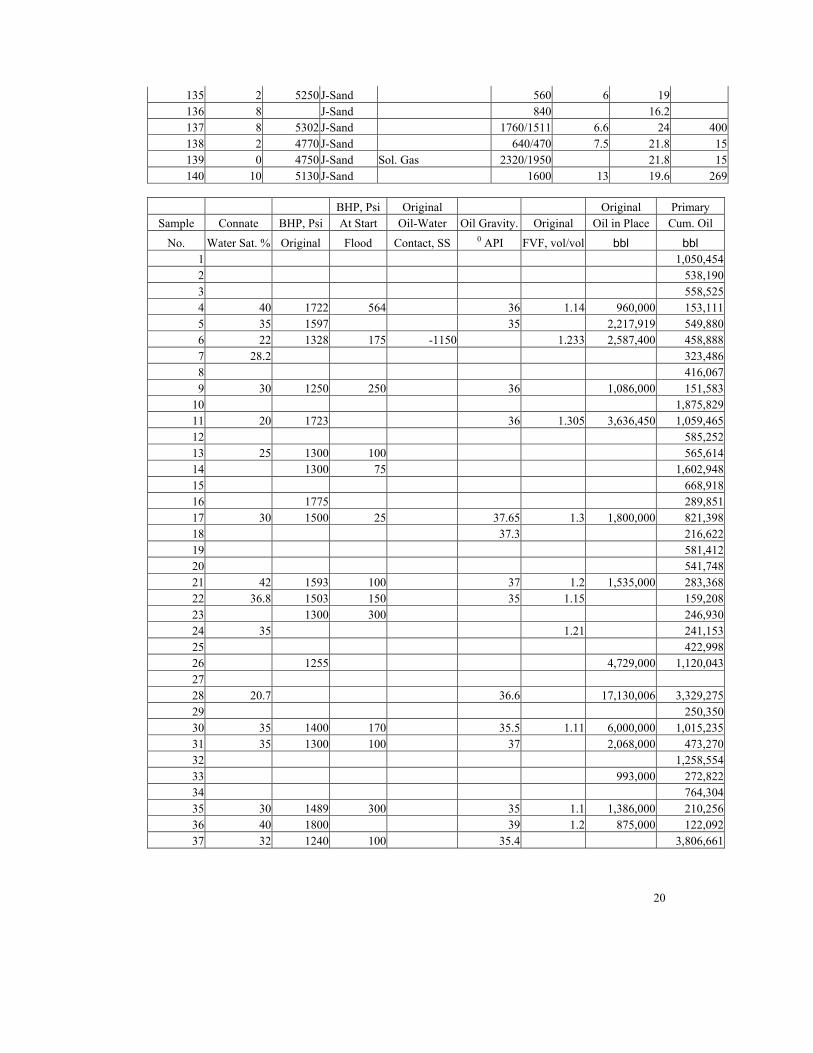
20

135 2 5250 J-Sand 560 6 19 136 8 J-Sand 840 16.2 137 8 5302 J-Sand 1760/1511 6.6 24 400138 2 4770 J-Sand 640/470 7.5 21.8 15139 0 4750 J-Sand Sol. Gas 2320/1950 21.8 15140 10 5130 J-Sand 1600 13 19.6 269

BHP, Psi Original Original Primary

Sample Connate BHP, Psi At Start Oil-Water Oil Gravity. Original Oil in Place Cum. Oil

No. Water Sat. % Original Flood Contact, SS 0 API FVF, vol/vol bbl bbl 1 1,050,4542 538,1903 558,5254 40 1722 564 36 1.14 960,000 153,1115 35 1597 35 2,217,919 549,8806 22 1328 175 -1150 1.233 2,587,400 458,8887 28.2 323,4868 416,0679 30 1250 250 36 1,086,000 151,583

10 1,875,82911 20 1723 36 1.305 3,636,450 1,059,46512 585,25213 25 1300 100 565,61414 1300 75 1,602,94815 668,91816 1775 289,85117 30 1500 25 37.65 1.3 1,800,000 821,39818 37.3 216,62219 581,41220 541,74821 42 1593 100 37 1.2 1,535,000 283,36822 36.8 1503 150 35 1.15 159,20823 1300 300 246,93024 35 1.21 241,15325 422,99826 1255 4,729,000 1,120,04327 28 20.7 36.6 17,130,006 3,329,27529 250,35030 35 1400 170 35.5 1.11 6,000,000 1,015,23531 35 1300 100 37 2,068,000 473,27032 1,258,55433 993,000 272,82234 764,30435 30 1489 300 35 1.1 1,386,000 210,25636 40 1800 39 1.2 875,000 122,09237 32 1240 100 35.4 3,806,661

21

38 37.5 38 1,002,000 443,80439 1,276,77540 25 1115 633 -445 36.7 1.26 9,641,000 509,02641 58 1300 400 -603 36 1.2 3,430,000 391,97942 308,81943 409,93344 32.5 1290 200 37 1.156 2,636,400 492,61645 40 958 37 1.1 922,000 115,12746 28 1300 250 37 1.2 3,492,500 1,199,71547 36.6 892 1.1515 5,546,000 783,24148 35.3 853,50649 1,557,04050 1250 531,49451 1020 180 1,009,55352 40 1172 1.15 1,764,000 279,72753 2,200,000 201,42454 40 1100 150 37 1.23 1,710,000 434,80755 678,96856 37 5,200,000 1,262,82257 -576 3,500,000 76,60358 1000 700 3,740,000 1,332,05059 1240 200 3,200,000 544,56760 2,841,30861 1175 305,90462 29 1666 110 37 1.17 6,477,000 660,81263 104,00764 1,901,63665 30 1512 260 39 1.25 4,258,000 718,46866 30 1512 39 1.25 2,100,000 397,23267 56 1590 100 39 1.18 2,155,000 611,11368 48 1355 1.25 917,000 351,81069 30 1546 250 -1975 39.2 1.2 3,240,000 704,63270 1249 352 -1035 6,261,250 968,54971 30 1650 700 -1916 33 1.25 3,530,000 636,79472 40 1640 327 38.5 1.3 3,604,279 667,70073 30 1270 38 5,560,000 74 394,81575 389,52276 56.48 1942 300 882,500 106,02677 1700 200 500,068 110,97278 25 1600 100 1.27 2,200,000 483,43179 34 1594 100 38.7 623,000 136,13380 29.2 1.24 1,268,300 234,84481 2,915,65582 119,50683 24 1240 250 -1000 39 1.174 1,105,88584 344,323

22

85 347,30786 1500 250 1,869,89687 36 39 1.3 2,100,000 365,45388 1.13 112,60589 206,68790 35 1375 150 -1292 39 1.2 6,276,000 1,351,18691 35 1.15 291,45392 20 1380 100 35 1.15 725,000 258,00893 200 303,90994 -1785 3,626,52995 218,13496 25 1460 100 39 1.13 2,521,000 507,65997 52 1300 700 38 1.15 270,98698 2,827,66099 1300 650 2,635,000 352,121

100 384,924101 28 1500 150 38 1.25 26,050,000 3,722,269102 35 1655 38 1.3 1,187,000 204,298103 35 1525 38 1.3 1,390,000 251,005104 446,015105 20 1400 50 37 1.2 926,000 354,919106 1434 400 36 1,875,000 129,301107 200 4,062,702108 35 1200 37 1.25 1,136,670 497,342109 38 1500 500 38 1.1 2,756,248 167,166110 32.5 381,662111 200 60,000,000 968,996112 1417 100 1,600,000 287,737113 35 340,000 159,279114 153,212115 4,509,192116 1,900,000 645,229117 38 1510 200 40 1.3 573,562 173,376118 169,383119 649,857120 44.1 233,841121 3,604,000 1,188,532122 41.5 1410 1.2 1,228,800 144,341123 1,261,337124 30 1475 85 37 1.33 6,000,000 1,193,818125 35 1430 100 37 3,000,000 506,111126 40 1425 210 -1348 39 1.22 1,500,000 279,272127 27 1410 36 1.25 3,094,000 363,052128 25 1.12 866,333129 40 905 34 1,061,000 281,949130 1,810,800 263,918131 1090 670 481,455

23

132 482,360133 1,385,303134 234,599135 2,185,234 657,091136 40 1100 200 1.098 1,014,015 164,529137 25 1200 100 -876 36.4 1.2 11,396,000 3,101,320138 41 1350 300 36 1.3 2,693,000 207,463139 41 1350 400 -820 36 1.3 14,699,000 927,299140 23 1259 1.09 11,798,000 934,184

Primary Primary Cum. Prod. Cum. Prod. Cum. Prod.

Sample Cum. Gas Cum. Water Max Prod. P+S P+S P+S Primary Primary

No. mcf bbl Rate, BOPM Cum. Oil Cum. Gas Cum. Water Cum. GOR Cum. WOR1 558,793 132,898 3,413,228 1,084,827 6,069,245 1.88 0.132 336,123 197,147 538,661 336,726 208,965 1.60 0.373 443,803 80,963 1,314,445 738,041 1,274,826 1.26 0.144 15,004 94,694 175,022 15,004 178,933 10.20 0.625 141,078 795,195 596,576 142,606 826,331 3.90 1.456 54,809 10,197 60,000 715,826 100,193 2,519,761 8.37 0.027 43,289 1,738 430,775 46,199 111,556 7.47 0.018 226,552 26,624 1,422,796 768,193 1,968,888 1.84 0.069 57,247 1,996 9,000 190,853 72,435 33,757 2.65 0.01

10 487,234 26,344 2,686,942 1,054,011 2,546,438 3.85 0.0111 167,644 1,874 64,000 1,934,595 1,100,399 9,851,974 6.32 0.0012 234,574 257,155 926,710 319,363 8,055,768 2.49 0.4413 137,765 12,535 19,000 638,003 145,364 55,259 4.11 0.0214 512,647 100,139 3,607,337 638,456 14,864,084 3.13 0.0615 337,519 56,258 1,696,426 663,889 2,124,701 1.98 0.0816 7,781 20,814 533,411 7,781 1,022,466 37.25 0.0717 568,838 51,446 858,148 606,338 126,868 1.44 0.0618 123,320 414,237 224,318 123,320 446,265 1.76 1.9119 86,590 508,708 629,435 86,590 640,311 6.71 0.8720 108,098 26,866 1,012,874 183,073 1,311,569 5.01 0.0521 115,638 16,741 415,317 115,638 220,227 2.45 0.0622 65,987 438,851 240,475 65,987 5,787,026 2.41 2.7623 139,955 128,248 487,819 250,636 852,026 1.76 0.5224 128,248 77,580 20,000 338,348 112,843 215,334 1.88 0.3225 300,702 13,971 589,990 559,285 250,689 1.41 0.0326 323,888 242,976 28,000 1,653,067 323,888 9,109,507 3.46 0.2227 872,457 440,397 465,239 28 1,382,749 71,886 164,000 9,781,926 1,853,302 73,438,165 2.41 0.0229 166,513 16,081 7,600 391,373 202,018 97,001 1.50 0.0630 148,079 936,964 1,500 1,709,090 217,861 7,094,093 6.86 0.9231 1,874 12,469 10,000 927,640 1,874 919,287 252.55 0.0332 729,591 36,131 3,324,348 1,392,777 3,268,195 1.73 0.0333 28,059 418,939 343,678 28,059 824,461 9.72 1.5434 373,050 19,006 4,000 2,842,261 708,638 5,083,931 2.05 0.02

24

35 0 24,376 376,564 0 330,294 0.1236 15,332 7,639 6,400 211,922 23,019 95,763 7.96 0.0637 2,343,081 173,116 8,273,069 2,720,281 37,291,191 1.62 0.0538 75,087 12,218,177 450,351 75,089 12,210,177 5.91 27.5339 4,553 3,261,713 27,000 1,718,405 4,553 10,461,303 280.42 2.5540 624,139 0 60,000 4,061,335 6,721,631 11,450,372 0.82 0.0041 190,792 216,185 1,008,651 190,792 2,445,317 2.05 0.5542 18,827 365,157 314,109 18,827 372,364 16.40 1.1843 64,653 1,403,489 503,127 65,053 4,085,171 6.34 3.4244 215,942 23,115 15,000 900,303 290,366 2,300,882 2.28 0.0545 36,761 96,625 244,511 60,332 674,101 3.13 0.8446 376,493 491,884 1,740,703 376,490 10,341,538 3.19 0.4147 0 188,083 2,345,466 0 8,010,618 0.2448 392,167 12,920 21,000 1,802,099 443,404 2,570,881 2.18 0.0249 913,366 85,353 49,000 2,834,296 1,065,172 7,119,272 1.70 0.0550 180,659 307,239 665,190 180,659 1,029,431 2.94 0.5851 70,933 1,143,358 29,000 1,312,423 164,122 5,438,606 14.23 1.1352 7,832 34,080 5,000 291,269 74,471 134,802 35.72 0.1253 65,005 126,918 12,000 461,259 360,749 912,736 3.10 0.6354 201,887 67,256 13,000 660,302 220,266 1,594,714 2.15 0.1555 285,836 98,309 1,194,924 300,826 2,372,829 2.38 0.1456 84,057 213,804 24,000 3,312,264 4,375,718 17,184,662 15.02 0.1757 183,081 2,616,313 15,000 86,092 190,226 3,281,468 0.42 34.1558 724,858 2,773,427 1,361,781 724,858 3,105,627 1.84 2.0859 106,036 985,278 664,561 114,019 2,614,455 5.14 1.8160 2,418,782 12,664,397 2,942,869 2,431,186 16,077,343 1.17 4.4661 178,791 56,683 515,399 223,861 1,557,578 1.71 0.1962 251,403 255,282 698,316 279,762 588,734 2.63 0.3963 0 469,116 151,700 0 1,159,491 4.5164 795,248 228,509 4,178,477 1,054,679 22,508,694 2.39 0.1265 243,952 19,927 32,000 1,220,955 251,211 6,653,114 2.95 0.0366 102,620 6,818 507,323 168,092 200,577 3.87 0.0267 40,947 6,650,854 625,760 47,890 6,701,823 14.92 10.8868 264,197 14,050 19,000 551,943 272,155 1,252,145 1.33 0.0469 118,049 280,094 1,350 928,767 138,012 1,410,473 5.97 0.4070 61,330 1,318,081 1,005,781 61,330 2,185,321 15.79 1.3671 143,548 364,448 1,200 657,759 154,198 560,453 4.44 0.5772 334,247 172,709 838,291 435,150 917,451 2.00 0.2673 354,655 221,955 1,453,210 543,692 1,078,180 0.00 74 322,820 12,983 405,561 324,624 124,944 1.22 0.0375 389,522 41,487 440,930 23,146 524,940 1.00 0.1176 165,480 11,179 194,076 261,739 347,923 0.64 0.1177 11,359 390,067 111,179 11,359 406,249 9.77 3.5278 173,398 5,104 12,120 664,663 218,818 520,323 2.79 0.0179 79,109 15,243 11,000 147,297 91,554 26,740 1.72 0.1180 481,716 440,013 258,273 540,417 1,030,061 0.49 1.8781 320,984 54,824 9,180,887 1,392,728 20,337,563 9.08 0.02

25

82 1,255 5,539 130,960 1,709 12,086 95.22 0.0583 372,503 48,479 20,000 2,411,428 605,206 12,409,885 2.97 0.0484 129,994 1,790 1,402,897 386,953 1,170,384 2.65 0.0185 138,718 0 808,919 160,726 4,246,554 2.50 0.0086 703,794 550,127 74,000 3,310,478 796,196 9,156,515 2.66 0.2987 333,441 137,805 14,000 402,216 353,827 465,376 1.10 0.3888 14,898 33,567 4,200 121,341 14,898 43,409 7.56 0.3089 117,618 19,007 800 217,682 131,878 76,080 1.76 0.0990 217,967 33,869 15,000 2,709,594 217,967 8,047,108 6.20 0.0391 1,486 110,220 8,000 544,938 15,600 1,336,052 196.13 0.3892 39,718 3,820 500 261,035 39,718 3,859 6.50 0.0193 1,736,464 117,586 600 684,830 5,382,913 904,856 0.18 0.3994 857,884 564,665 6,793,603 1,348,985 31,374,061 4.23 0.1695 22,057 283,453 7,500 230,629 27,757 428,213 9.89 1.3096 307,517 19,401 15,000 768,002 93,962 626,316 1.65 0.0497 11,446 176,585 284,920 11,446 224,466 23.68 0.6598 882,623 277,807 5,387,714 1,368,677 14,903,283 3.20 0.1099 11,497 234,003 445,357 11,494 770,875 30.63 0.66

100 4,546 371,437 448,791 4,546 779,696 84.67 0.96101 2,477,217 376,068 121,500 5,789,839 2,544,440 45,157,015 1.50 0.10102 91,251 7,458 256,687 128,620 290,167 2.24 0.04103 156,089 3,254 349,680 210,648 102,291 1.61 0.01104 74,019 9,665 1,947,743 320,111 4,260,014 6.03 0.02105 54,666 74,092 703,284 54,666 2,971,951 6.49 0.21106 152,332 55,455 18,000 308,926 176,601 956,043 0.85 0.43107 1,079,156 5,459,221 4,386,202 1,145,541 8,725,533 3.76 1.34108 118,677 52,782 950 737,039 118,677 108,873 4.19 0.11109 88,473 13,786 5,000 213,408 102,580 104,239 1.89 0.08110 36,165 103,244 610,883 80,371 1,133,057 10.55 0.27111 186,005 32,799 1,814,316 388,949 2,437,954 5.21 0.03112 204,644 349,792 287,737 204,644 349,792 1.41 1.22113 4,016 162,510 900 173,796 4,016 218,809 39.66 1.02114 12,728 14,038 188,829 30,061 68,809 12.04 0.09115 1,422,549 8,615 289,000 16,260,239 4,889,025 42,799,140 3.17 0.00116 288,584 1,914,845 15,200 854,307 299,006 3,333,391 2.24 2.97117 108,122 17,620 242,175 126,652 90,115 1.60 0.10118 44,624 430 444,995 68,923 878,153 3.80 0.00119 180,625 164,584 1,046,639 180,625 1,800,613 3.60 0.25120 129,090 52,494 277,960 130,420 68,538 1.81 0.22121 313,283 41,826 1,496,240 339,366 1,582,965 3.79 0.04122 13,944 148,648 5,000 196,253 16,973 1,207,659 10.35 1.03123 126,210 145,478 1,700 1,488,604 126,210 1,208,204 9.99 0.12124 70,607 28,392 51,000 1,800,899 107,717 2,354,446 16.91 0.02125 305,769 102,980 882,977 426,523 1,314,596 1.66 0.20126 74,909 65,821 402,672 76,205 484,173 3.73 0.24127 68,399 37,958 399,616 68,399 171,462 5.31 0.10128 3,266 153,725 19,000 1,073,437 58,002 3,631,743 265.26 0.18

26

129 39,140 2,121,317 5,000 355,115 53,610 3,071,533 7.20 7.52130 50,307 194,146 1,400 294,974 65,030 217,046 5.25 0.74131 95,229 44,278 30,000 777,844 114,873 3,794,181 5.06 0.09132 34,512 175,458 30,000 986,235 94,975 4,663,746 13.98 0.36133 416,950 486,565 1,752,937 434,602 4,923,540 3.32 0.35134 104,491 9,405 13,000 407,009 111,882 262,982 2.25 0.04135 100,282 112,662 697,607 101,572 115,898 6.55 0.17136 3,988 110,074 181,765 5,552 184,367 41.26 0.67137 82,916 83,125 125,000 5,101,320 216,641 36,348,769 37.40 0.03138 58,158 575 6,000 318,196 218,861 153,937 3.57 0.00139 267,286 13,299 315,000 2,073,435 1,425,787 3,970,320 3.47 0.01140 233,272 36,044 77,000 2,176,324 307,372 3,967,209 4.00 0.04

27

Appendix B

28

A brief overview of the concepts of fuzzy ranking and neural networks was included in the original statement of work. It is repeated for completeness in appendix B. Fuzzy Ranking & Neural Network Background Earlier attempts by others to correlate oil recovery with public information focused on the effect of a single variable with recovery. Correlating two variables in this manner with a x-y cross plot is an uni-variant analysis. A uni-variant correlation between API gravity, depth, reservoir thickness, porosity, number of producing wells, number of dry holes, well spacing, formation volume factor, gas-oil ratio, water-oil ratio, original bottom hole pressure, bottom hole pressure at the end of primary, connate water saturation, original oil place, discovery date, unitization date, initial producing rate (gas, oil, water), or cumulative primary production (gas, oil, water) with S/P might be tenuous at best. If a multivariable technique is used to establish the relationships, the correlations can be robust. Neural networks are useful for correlating more than two variables. Neural nets work best when the dependent variables have a real bearing on the independent variable, that is the S/P ratio in this case. Selecting the strength of the dependent variables (21 are included in the previous paragraph) is objectively accomplished with a fuzzy ranking algorithm. The algorithm develops dimensionless cross plots of each dependent variable versus the S/P ratio. The cross plots are used to evaluate the correlation of each variable with S/P. For example, if the connate water saturation values vary very little with the S/P values from the ? projects it can be assumed that the Swc values are not strong correlating parameters. Similarly, the GOR prior to waterflooding may be inversely proportional to the S/P and GOR would be a strong dependent variable. All dependent variables will be evaluated in this manner. The fuzzy ranking cartoons in Figs. B1a & B1b illustrate the concept.

Figure B1a. Conventional cross plot of a random data set (0-1). No correlation between X and Y. The trend is 0.5 (average between 0 and 1) is not evident.

y=Random(x)

0.0

0.2

0.4

0.6

0.8

1.0

0.0 0.2 0.4 0.6 0.8 1.0

X

Y

29

Figure B1b. A Conventional cross plot of a random data set (0-1) plus a square root

trend. Note the apparent correlation. The bell shaped lines are fuzzy membership functions used to identify trends in what can appear to be random data. The fuzzy curves, a type of average of the points encompassed by the curve, are illustrated in Fig. B2 and clearly identify the trends not easily seen in the conventional cross plots. The range, change in Y value, of the random data is about 0.26, indicating no meaningful correlation. The range of the random data plus the square root trend is ~0.9, indicating a correlation between X and Y.

y=Random(x)+(x)^0.5

0.0

0.5

1.0

1.5

2.0

0.0 0.2 0.4 0.6 0.8 1.0

X

Y

30

Figure B2. Fuzzy ranking curves. The trends are clearly evident.

Fuzzy ranking technology was used to prioritize the descriptive parameters found in the waterflood hearing files. A neural network was used to correlate the highest-ranking parameters with S/P. Correlate the highest-ranking parameters with the S/P

Neural networks are useful for correlating more than two variables. They can be viewed as an inverse problem solver where a system of non-linear equations is developed to yield a known value, in this case the S/P ratio. The variables in the equations are the high-ranking parameters. The constants in the equations are called weights. During the training of a neural network, the weights are adjusted to yield the S/P value known from field performance.

A non-linear, feed forward, back propagation, neural network with a fast matrix solver was used to correlate the highest-ranking variables with S/P as the independent variable. Fully connected neural network architectures were evaluated for speed and efficiency. As an example, two different neural network architectures (4-4-2-1 and 4-3-2-1) are seen in Fig. B3. A1, A2, A3, and A4 are the highest ranking input variables, any number of inputs can be used. The tie lines are the weights and circles are the non-linearity functions. Maintaining a satisfactory ratio of training data to weights

Fuzzy Curves and Their Trends

0.0

0.2

0.4

0.6

0.8

1.0

1.2

1.4

1.6

1.8

0.0 0.2 0.4 0.6 0.8 1.0

X

Y

31

(coefficients of the regression equation) is assured since there are 42 S/P values for training with perhaps 50 weights depending on the number of high ranking variables selected as input. A good overview of a back propagation neural network is available at http://www.npto.doe.gov/Software/miscindx.html see the Risk Analysis manual.

Figure B4. Example of Neural Network Architectures. Neural networks are trained to yield an output value (S/P in this case). The goodness of the training is expressed as a correlation coefficient with 100% being perfect. In reality networks trained to about 80% are suitable for forecasting. Once a network is trained it can be used to predict the S/P of any non-flooded field given the input parameters. The accuracy of the predictions can be judged with exclusion testing. A parsed dataset consisting of ? of the known ? S/P values was used to train the best neural network architecture. The ? values dataset network will be used to predict the ? excluded values. The goodness of the predictions will be estimated with a forecast versus actual cross-plot. Exclusion testing provides a means of estimating the validity of the correlations. However, the Cliff Farms Unit waterflood reserves are based on the neural network trained with ? S/P data points.

Fig. B4a&b illustrates exclusion testing as a validation tool. The two variable cross-plot, titled 1-1 Architecture in Fig. B4a, has little value as a forecasting tool. The additional information included in the multi-variable neural network correlation, titled 4-4-3-1 Architecture, resulted in a robust correlation able to forecast with an 88% correlation coefficient.

Architecture(4-4-2-1)

A1

A2

A3

A4

S/P

Architecture(4-3-2-1)

A1

A2

A3

A4

S/P

32

Figures B5a & b. Exclusion testing with a simple architecture versus a complex architecture on the right.

Unshifted 4-4-3-1 Architecture

0

5

10

15

20

0 5 10 15 20

Core Plug φ, %

Pred

icte

d φ,

%

88 % cc

Unshifted 1-1 Architecture

0

5

10

15

20

25

30

0 10 20 30

Core Plug φ, %

Pred

icte

d φ,

% 45 % cc