Embed Size (px)
Citation preview

Smart Home Technologies
Data Mining and Prediction
Objectives of Data Mining and Prediction
� Large amounts of sensor data have to be “interpreted” to acquire knowledge about tasks that occur in the environment
� Patterns in the data can be used to predict future events
� Knowledge of tasks facilitates the automation of task components to improve the inhabitants’ experience

Data Mining and Prediction
� Data Mining attempts to extract patterns from the available data
� Associative patterns
What data attributes occur together ?
� Classification
What indicates a given category ?
� Temporal patterns
What sequences of events occur frequently ?

Example Patterns
� Associative patternWhen Bob is in the living room he likes to watch TV and eat popcorn with the light turned off.
� ClassificationAction movie fans like to watch Terminator, drink beer, and have pizza.
� Sequential patternsAfter coming out of the bedroom in the morning, Bob turns off the bedroom lights, then goes to the kitchen where he makes coffee, and then leaves the house.
Data Mining and Prediction
� Prediction attempts to form patterns that permit it to predict the next event(s)
given the available input data.
� Deterministic predictions
If Bob leaves the bedroom before 7:00 am on a
workday, then he will make coffee in the kitchen.
� Probabilistic sequence models
If Bob turns on the TV in the evening then he will 80% of the time go to the kitchen to make popcorn.
Objective of Prediction in Intelligent Environments
� Anticipate inhabitant actions
� Detect unusual occurrences (anomalies)
� Predict the right course of actions
� Provide information for decision making
� Automate repetitive tasks
e.g.: prepare coffee in the morning, turn on lights
� Eliminate unnecessary steps, improve sequencese.g.: determine if will likely rain based on weather forecast and external sensors to decide if to water the lawn.

What to Predict
� Behavior of the Inhabitants
� Location
� Tasks / goals
� Actions
� Behavior of the Environment
� Device behavior (e.g. heating, AC)
� Interactions

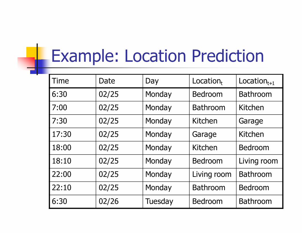
Example: Location Prediction
� Where will Bob go next?
� Locationt+1 = f(x)
� Input data x:
� Locationt, Locationt-1, …
� Time, date, day of the week
� Sensor data

Example: Location Prediction
Time Date Day Locationt Locationt+1
6:30 02/25 Monday Bedroom Bathroom
7:00 02/25 Monday Bathroom Kitchen
7:30 02/25 Monday Kitchen Garage
17:30 02/25 Monday Garage Kitchen
18:00 02/25 Monday Kitchen Bedroom
18:10 02/25 Monday Bedroom Living room
22:00 02/25 Monday Living room Bathroom
22:10 02/25 Monday Bathroom Bedroom
6:30 02/26 Tuesday Bedroom Bathroom

Example: Location Prediction
� Learned pattern
� If Day = Monday…Friday
& Time > 0600
& Time < 0700
& Locationt = Bedroom
Then Locationt+1 = Bathroom
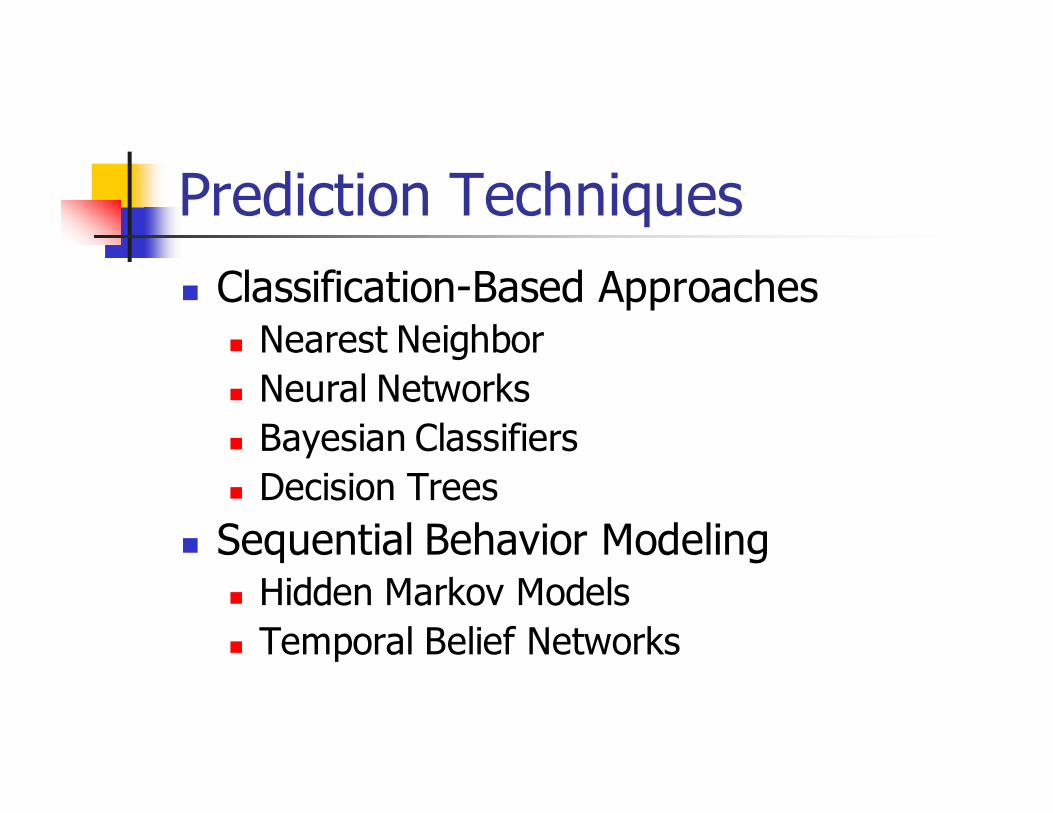
Prediction Techniques
� Classification-Based Approaches� Nearest Neighbor
� Neural Networks
� Bayesian Classifiers
� Decision Trees
� Sequential Behavior Modeling� Hidden Markov Models
� Temporal Belief Networks

Classification-Based Prediction
� Problem� Input: State of the environment
� Attributes of the current state inhabitant location, device status, etc.
� Attributes of previous states
� Output: Concept description� Concept indicates next event
� Prediction has to be applicable to future examples

Instance-Based Prediction: Nearest Neighbor
� Use previous instances as a model for future instances
� Prediction for the current instance is chosen as the classification of the most similar previously observed instance.� Instances with correct classifications (predictions) (xi,f(xi)) are stored
� Given a new instance xq, the prediction is derived as the one of the most similar instance xk:
f(xq) = f(xk)

Example: Location Prediction
Time Date Day Locationt Locationt+1
6:30 02/25 Monday Bedroom Bathroom
7:00 02/25 Monday Bathroom Kitchen
7:30 02/25 Monday Kitchen Garage
17:30 02/25 Monday Garage Kitchen
18:00 02/25 Monday Kitchen Bedroom
18:10 02/25 Monday Bedroom Living room
22:00 02/25 Monday Living room Bathroom
22:10 02/25 Monday Bathroom Bedroom
6:30 02/26 Tuesday Bedroom Bathroom
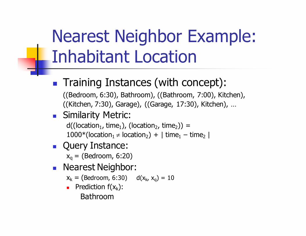
Nearest Neighbor Example: Inhabitant Location
� Training Instances (with concept):((Bedroom, 6:30), Bathroom), ((Bathroom, 7:00), Kitchen),
((Kitchen, 7:30), Garage), ((Garage, 17:30), Kitchen), …
� Similarity Metric:d((location1, time1), (location2, time2)) =
1000*(location1 ≠ location2) + | time1 – time2 |
� Query Instance:xq = (Bedroom, 6:20)
� Nearest Neighbor:xk = (Bedroom, 6:30) d(xk, xq) = 10
� Prediction f(xk):
Bathroom
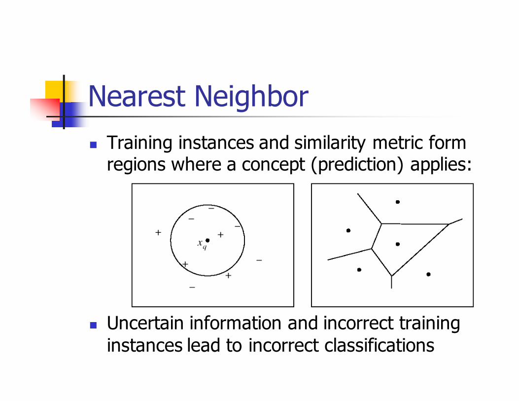
Nearest Neighbor
� Training instances and similarity metric form regions where a concept (prediction) applies:
� Uncertain information and incorrect training
instances lead to incorrect classifications

k-Nearest Neighbor
� Instead of using the most similar instance, use the average of the k most similar
instances
� Given query xq, estimate concept (prediction) using majority of k nearest neighbors
� Or, estimate concept by establishing the concept with the highest sum of inverse distances:
∑=∈
=ffki qi
f
x di xx
w)(, ),(
1

k-Nearest Neighbor Example
� TV viewing preferences
� Distance Function?� What are the important attributes ?
� How can they be compared ?
Time Date Day Channel Genre Title
19:30 02/25 Thursday 27 Reality Cops
21:00 02/25 Thursday 33 News News
19:00 02/26 Friday 11 News News
12:00 02/27 Saturday 21 Action Terminator I
20:00 02/27 Saturday 8 News News
… … … … … …
Time Date Day Channel Genre Title
13:30 03/20 Sunday 13 Reality Antiques Roadshow
22:00 03/20 Sunday 4 News News
20:00 03/21 Monday 8 News 60 Minutes
22:00 03/22 Tuesday 13 Documentary Nova
… … … … … …
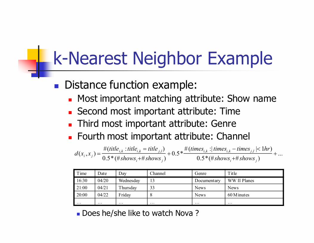
k-Nearest Neighbor Example
� Distance function example:� Most important matching attribute: Show name
� Second most important attribute: Time
� Third most important attribute: Genre
� Fourth most important attribute: Channel
...)#(#*5.0
)1|:|(#*5.0
)#(#*5.0
):(#),(
,,,,,, ++
<−+
+
==
ji
ljkiki
ji
ljkiki
jishowsshows
hrtimestimestimes
showsshows
titletitletitlexxd
Time Date Day Channel Genre Title
16:30 04/20 Wednesday 13 Documentary WW II Planes
21:00 04/21 Thursday 33 News News
20:00 04/22 Friday 8 News 60 Minutes
… … … … … …
� Does he/she like to watch Nova ?
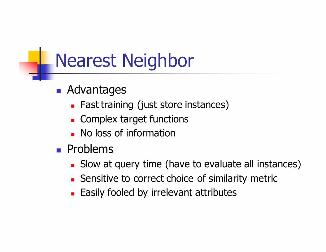
Nearest Neighbor
� Advantages
� Fast training (just store instances)
� Complex target functions
� No loss of information
� Problems
� Slow at query time (have to evaluate all instances)
� Sensitive to correct choice of similarity metric
� Easily fooled by irrelevant attributes

Decision Trees
� Use training instances to build a sequence of evaluations that permits to determine the correct category (prediction)
If Bob is in the Bedroom then
if the time is between 6:00 and 7:00 then
Bob will go to the Bathroom
else
� Sequence of evaluations are represented as a tree where leaves are labeled with the category
M
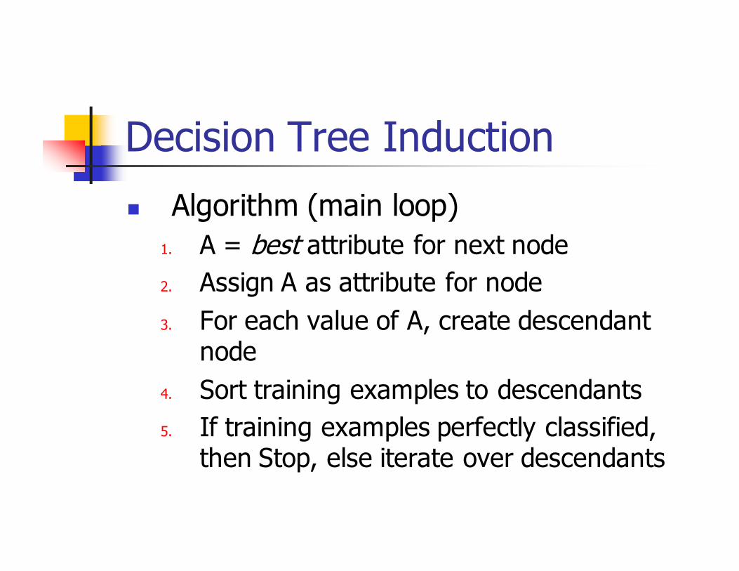
Decision Tree Induction
� Algorithm (main loop)
1. A = best attribute for next node
2. Assign A as attribute for node
3. For each value of A, create descendant node
4. Sort training examples to descendants
5. If training examples perfectly classified, then Stop, else iterate over descendants
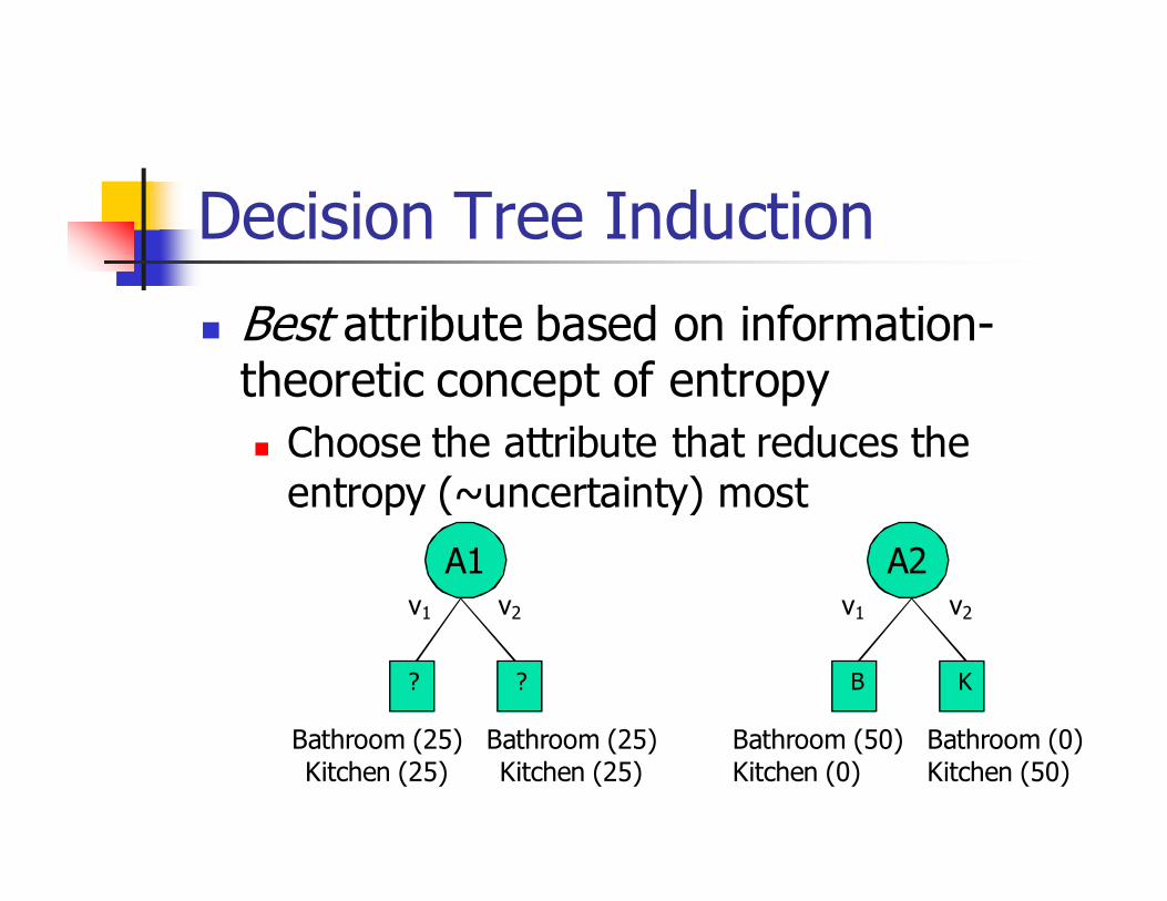
Decision Tree Induction
� Best attribute based on information-theoretic concept of entropy
� Choose the attribute that reduces the
entropy (~uncertainty) most
A1
Bathroom (25)
Kitchen (25)
Bathroom (25)
Kitchen (25)
? ?
v2v1
A2
Bathroom (0)
Kitchen (50)
Bathroom (50)
Kitchen (0)
B K
v1 v2
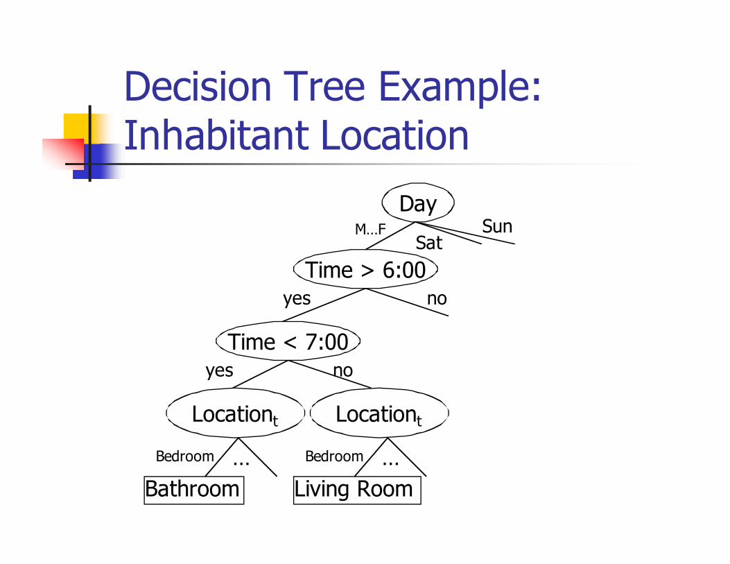
Decision Tree Example: Inhabitant Location
Day
Time > 6:00
Locationt
Time < 7:00
Bathroom
M…F
yes
yes
Bedroom …
no
no
SatSun
Locationt
Living Room
Bedroom …
Example: Location Prediction
Time Date Day Locationt Locationt+1
6:30 02/25 Monday Bedroom Bathroom
7:00 02/25 Monday Bathroom Kitchen
7:30 02/25 Monday Kitchen Garage
17:30 02/25 Monday Garage Kitchen
18:00 02/25 Monday Kitchen Bedroom
18:10 02/25 Monday Bedroom Living room
22:00 02/25 Monday Living room Bathroom
22:10 02/25 Monday Bathroom Bedroom
6:30 02/26 Tuesday Bedroom Bathroom
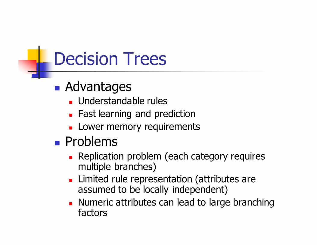
Decision Trees
� Advantages� Understandable rules
� Fast learning and prediction
� Lower memory requirements
� Problems� Replication problem (each category requires multiple branches)
� Limited rule representation (attributes are assumed to be locally independent)
� Numeric attributes can lead to large branching factors

Artificial Neural Networks
� Use a numeric function to calculate the correct category. The function is learned from
the repeated presentation of the set of
training instances where each attribute value is translated into a number.
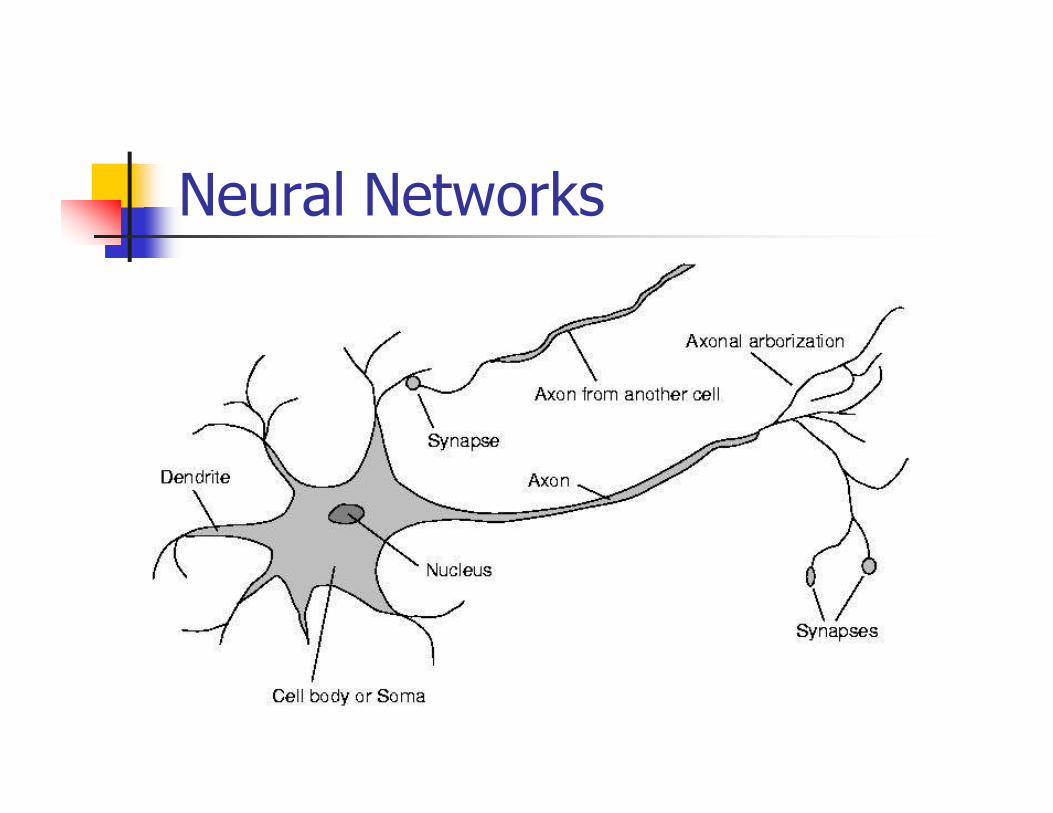
� Neural networks are motivated by the functioning of neurons in the brain.
� Functions are computed in a distributed fashion by a large number of simple computational units
Neural Networks
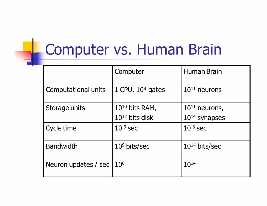
Computer vs. Human Brain
Computer Human Brain
Computational units 1 CPU, 108 gates 1011 neurons
Storage units 1010 bits RAM,
1012 bits disk
1011 neurons,
1014 synapses
Cycle time 10-9 sec 10-3 sec
Bandwidth 109 bits/sec 1014 bits/sec
Neuron updates / sec 106 1014
Artificial Neurons
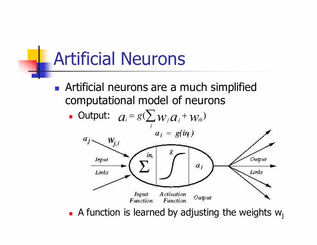
� Artificial neurons are a much simplified computational model of neurons
� Output:
� A function is learned by adjusting the weights wj
)( wawa thjj
jig += ∑
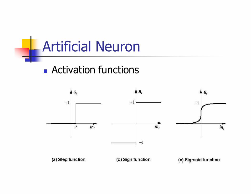
Artificial Neuron
� Activation functions
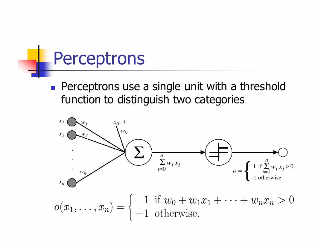
Perceptrons
� Perceptrons use a single unit with a threshold function to distinguish two categories
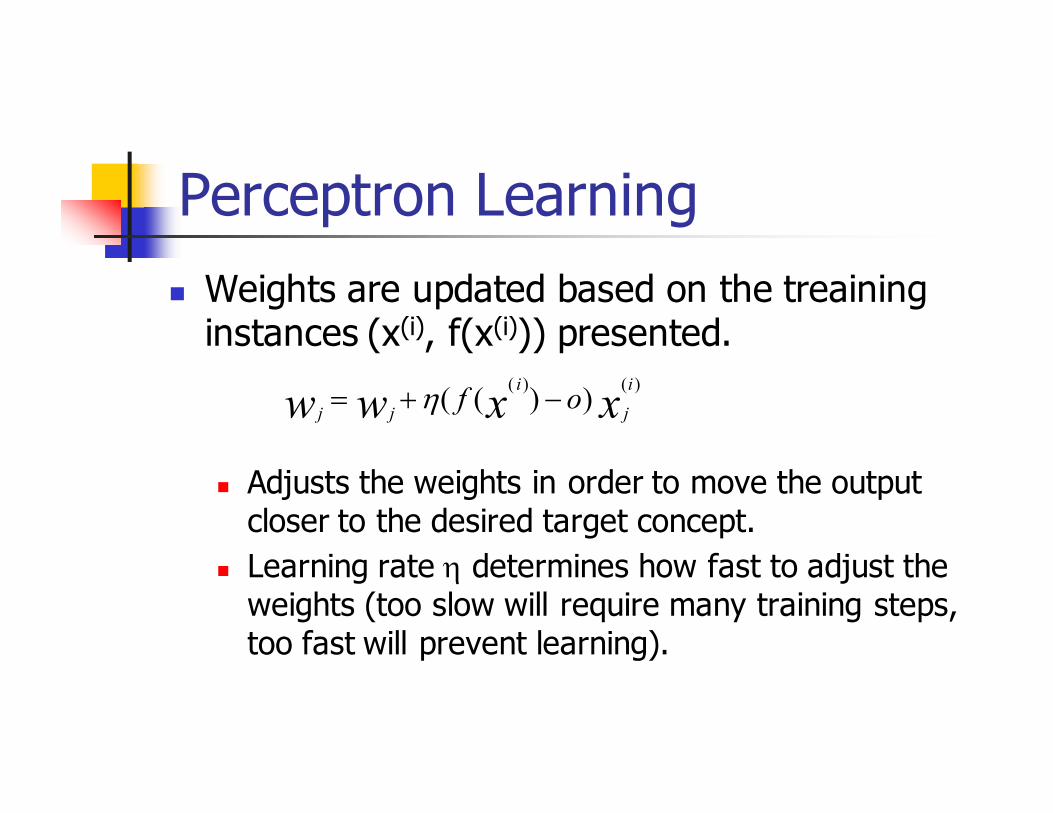
Perceptron Learning
� Weights are updated based on the treaining instances (x(i), f(x(i))) presented.
� Adjusts the weights in order to move the output closer to the desired target concept.
� Learning rate η determines how fast to adjust the weights (too slow will require many training steps, too fast will prevent learning).
xxwwi
j
i
jjof
)()())(( −+= η

Limitation of Perceptrons
� Learns only linearly-separable functions
� E.g. XOR can not be learned

Feed forward Networks with Sigmoid Units
� Networks of units with sigmoid activation functions can learn arbitrary functions
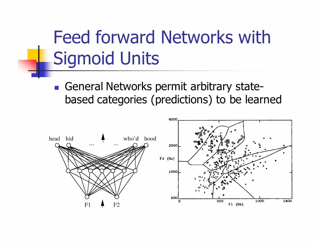
Feed forward Networks with Sigmoid Units
� General Networks permit arbitrary state-based categories (predictions) to be learned
Learning in Multi-Layer Networks: Error Back-Propagation
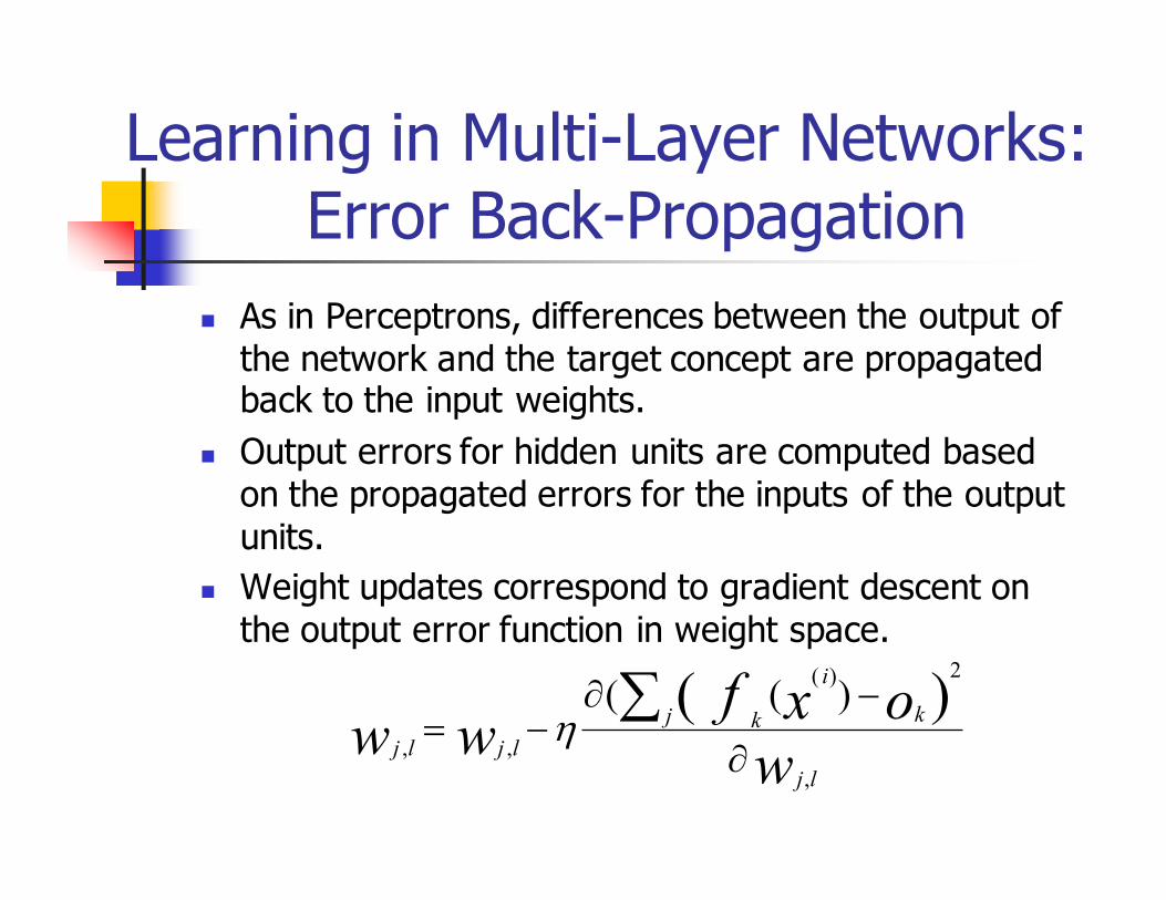
� As in Perceptrons, differences between the output of the network and the target concept are propagated back to the input weights.
� Output errors for hidden units are computed based on the propagated errors for the inputs of the output units.
� Weight updates correspond to gradient descent on the output error function in weight space.
woxf
wwlj
kj
i
k
ljlj
,
2)(
,,
)( )((
∂
−∂−=
∑η

Neural Network Examples
� Prediction
� Predict steering commands in cars
� Modeling of device behavior
� Face and object recognition
� Pose estimation
� Decision and Control
� Heating and AC control
� Light control
� Automated vehicles
Neural Network Example:Prediction of Lighting
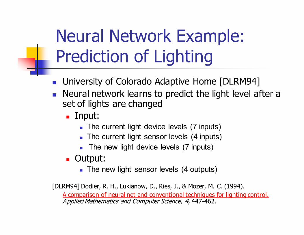
� University of Colorado Adaptive Home [DLRM94]
� Neural network learns to predict the light level after a set of lights are changed
� Input: � The current light device levels (7 inputs)
� The current light sensor levels (4 inputs)
� The new light device levels (7 inputs)
� Output:� The new light sensor levels (4 outputs)
[DLRM94] Dodier, R. H., Lukianow, D., Ries, J., & Mozer, M. C. (1994).
A comparison of neural net and conventional techniques for lighting control.Applied Mathematics and Computer Science, 4, 447-462.
Neural Networks
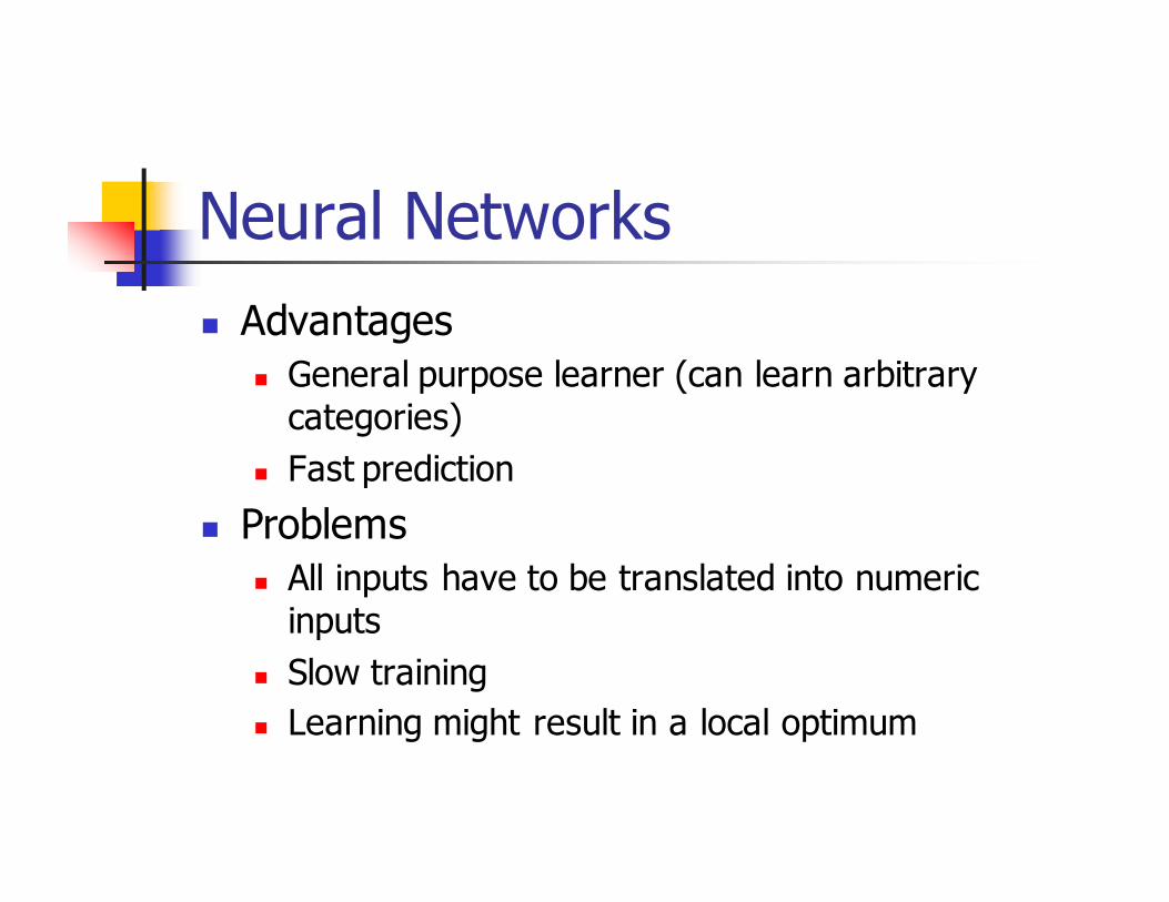
� Advantages
� General purpose learner (can learn arbitrary categories)
� Fast prediction
� Problems
� All inputs have to be translated into numeric inputs
� Slow training
� Learning might result in a local optimum
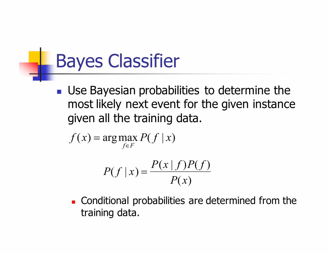
Bayes Classifier
� Use Bayesian probabilities to determine the most likely next event for the given instance
given all the training data.
� Conditional probabilities are determined from the training data.
)(
)()|()|(
xP
fPfxPxfP =
)|(maxarg)( xfPxfFf∈
=
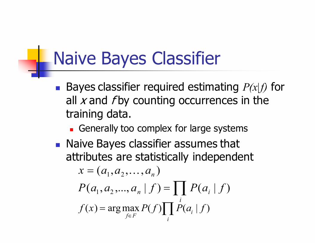
Naive Bayes Classifier
� Bayes classifier required estimating P(x|f) for
all x and f by counting occurrences in the training data.
� Generally too complex for large systems
� Naive Bayes classifier assumes that attributes are statistically independent
∏=i
in faPfaaaP )|()|,...,,( 21
∏∈
=i
iFf
faPfPxf )|()(maxarg)(
),,,( 21 naaax K=
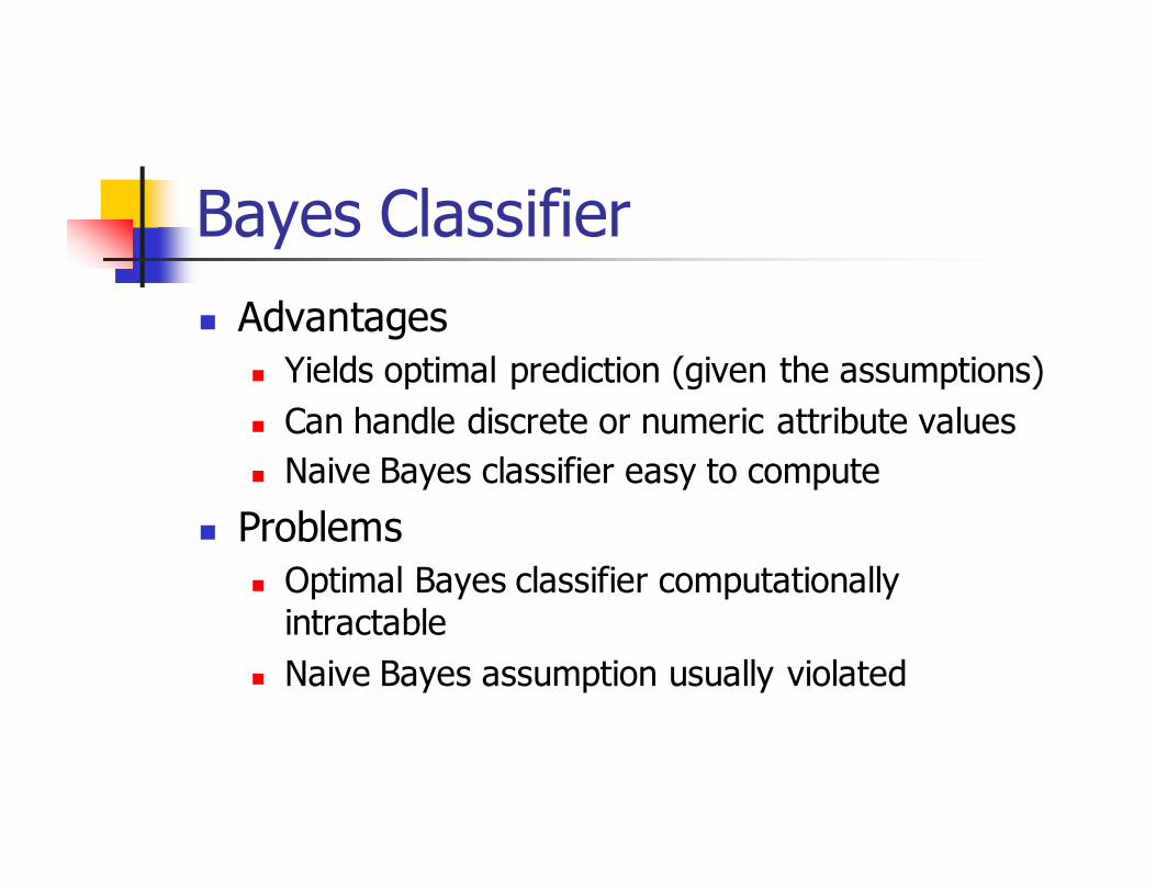
Bayes Classifier
� Advantages
� Yields optimal prediction (given the assumptions)
� Can handle discrete or numeric attribute values
� Naive Bayes classifier easy to compute
� Problems
� Optimal Bayes classifier computationally intractable
� Naive Bayes assumption usually violated

Bayesian Networks
� Bayesian networks explicitly represent the dependence and independence of various attributes.� Attributes are modeled as nodes in a network and links represent conditional probabilities.
� Network forms a causal model of the attributes
� Prediction can be included as an additional node.
� Probabilities in Bayesian networks can be calculated efficiently using analytical or statistical inference techniques.
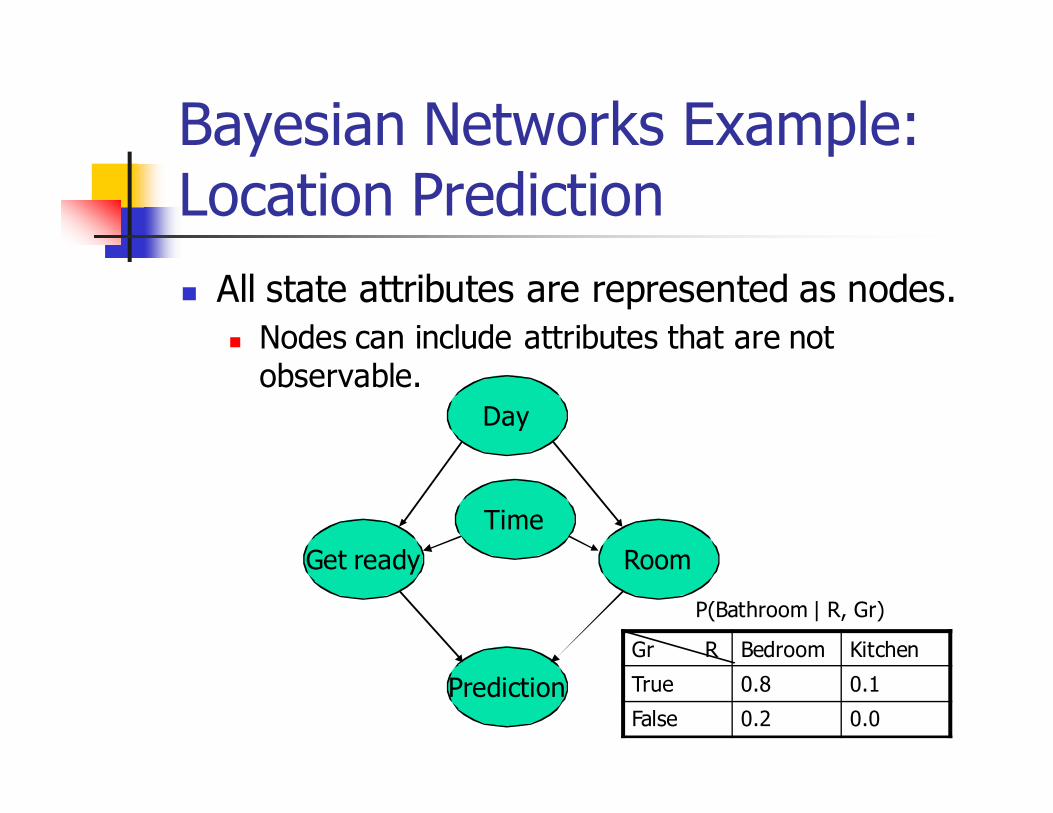
Bayesian Networks Example:Location Prediction
� All state attributes are represented as nodes.
� Nodes can include attributes that are not observable.
Prediction
RoomGet ready
Time
Day
Gr R Bedroom Kitchen
True 0.8 0.1
False 0.2 0.0
P(Bathroom | R, Gr)
Bayesian Networks
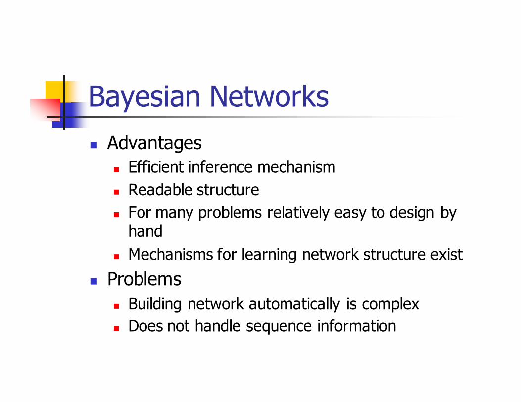
� Advantages
� Efficient inference mechanism
� Readable structure
� For many problems relatively easy to design by hand
� Mechanisms for learning network structure exist
� Problems
� Building network automatically is complex
� Does not handle sequence information

Sequential Behavior Prediction
� Problem� Input: A sequence of states or events
� States can be represented by their attributesinhabitant location, device status, etc.
� Events can be raw observationsSensor readings, inhabitant input, etc.
� Output: Predicted next event
� Model of behavior has to be built based on past instances and be usable for future predictions.
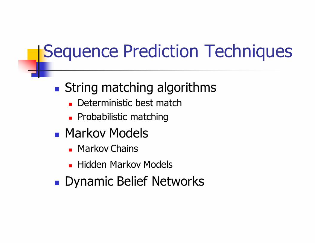
Sequence Prediction Techniques
� String matching algorithms� Deterministic best match
� Probabilistic matching
� Markov Models� Markov Chains
� Hidden Markov Models
� Dynamic Belief Networks
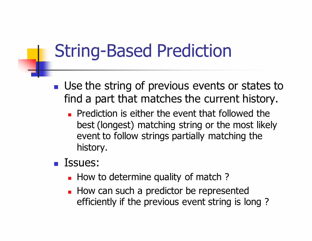
String-Based Prediction
� Use the string of previous events or states to find a part that matches the current history.
� Prediction is either the event that followed the best (longest) matching string or the most likely event to follow strings partially matching the history.
� Issues:
� How to determine quality of match ?
� How can such a predictor be represented efficiently if the previous event string is long ?

Example System: IPAM [DH98]
� Predict UNIX commands issued by a user
� Calculate p(xt,xt-1) based on frequency� Update current p(Predicted, xt-1) by α� Update current p(Observed, xt-1) by 1- α� Weight more recent events more heavily
� Data� 77 users, 2-6 months, >168,000 commands
� Accuracy less than 40% for one guess, but better than Naïve Bayes Classifier
[DH98] B. D. Davison and H. Hirsh. Probabilistic Online Action Prediction. Intelligent Environments: Papers from the AAAI 1998 Spring Symposium, Technical Report SS-98-02, pp. 148-154: AAAI Press.
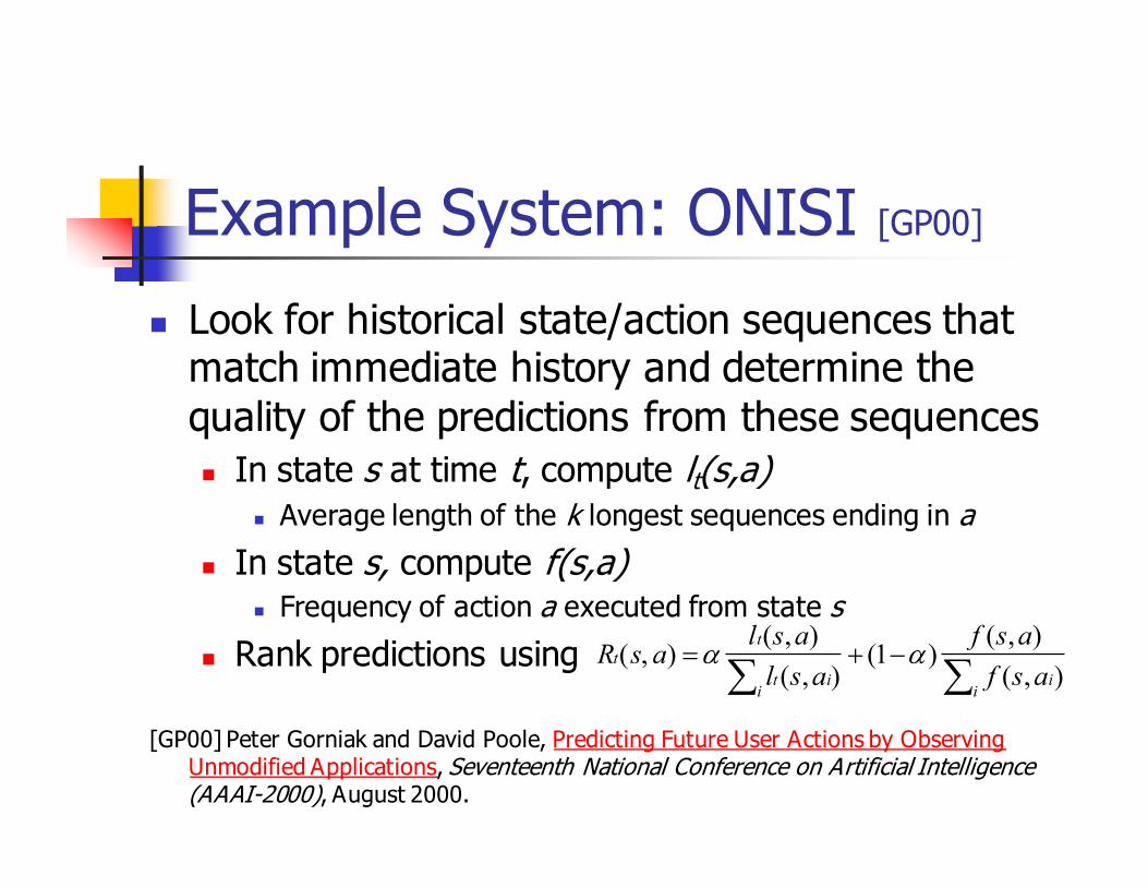
Example System: ONISI [GP00]
� Look for historical state/action sequences that match immediate history and determine the
quality of the predictions from these sequences
� In state s at time t, compute lt(s,a)� Average length of the k longest sequences ending in a
� In state s, compute f(s,a)� Frequency of action a executed from state s
� Rank predictions using
[GP00] Peter Gorniak and David Poole, Predicting Future User Actions by Observing Unmodified Applications, Seventeenth National Conference on Artificial Intelligence (AAAI-2000), August 2000.
∑∑−+=
ii
iit
t
t
asf
asf
asl
aslasR
),(
),()1(
),(
),(),( αα

Onisi Example [GP00]
� k=3, for action a3 there are only two matches of length 1 and 2, so lt(s3,a3) = (0+1+2)/3 = 1
� If α=0.9, the sum of averaged lengths for all actions is 5, a3 has occurred 50 times in s3, and
s3 is visited 100 times, then Rt(s3,a3) = 0.9*1/5 + 0.1*50/100 = 0.18+0.05 = 0.23

Example Sequence Predictors
� Advantages
� Permits predictions based on sequence of events
� Simple learning mechanism
� Problems
� Relatively ad hoc weighting of sequence matches
� Limited prediction capabilities
� Large overhead for long past state/action sequences
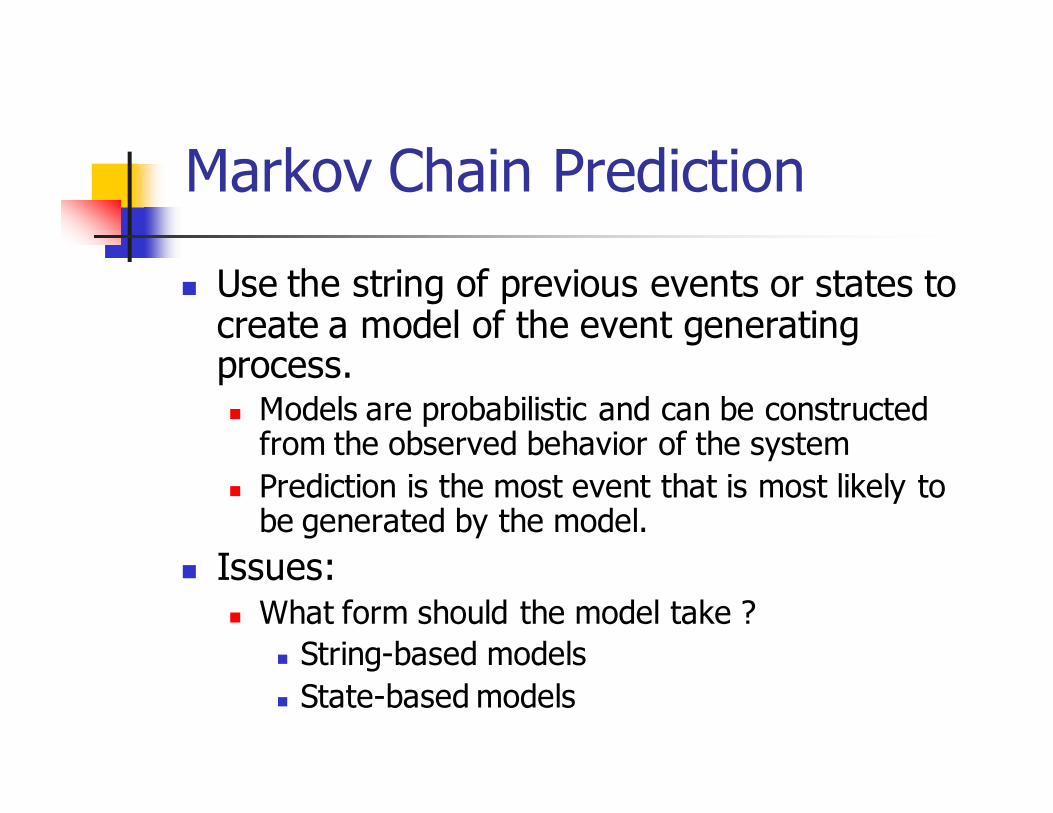
Markov Chain Prediction
� Use the string of previous events or states to create a model of the event generating process.� Models are probabilistic and can be constructed from the observed behavior of the system
� Prediction is the most event that is most likely to be generated by the model.
� Issues:� What form should the model take ?
� String-based models
� State-based models
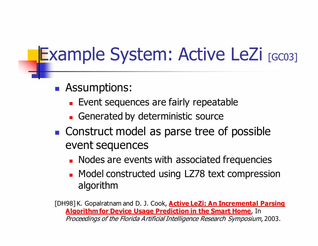
Example System: Active LeZi [GC03]
� Assumptions:
� Event sequences are fairly repeatable
� Generated by deterministic source
� Construct model as parse tree of possible
event sequences
� Nodes are events with associated frequencies
� Model constructed using LZ78 text compression algorithm
[DH98] K. Gopalratnam and D. J. Cook, Active LeZi: An Incremental Parsing Algorithm for Device Usage Prediction in the Smart Home, In Proceedings of the Florida Artificial Intelligence Research Symposium, 2003.
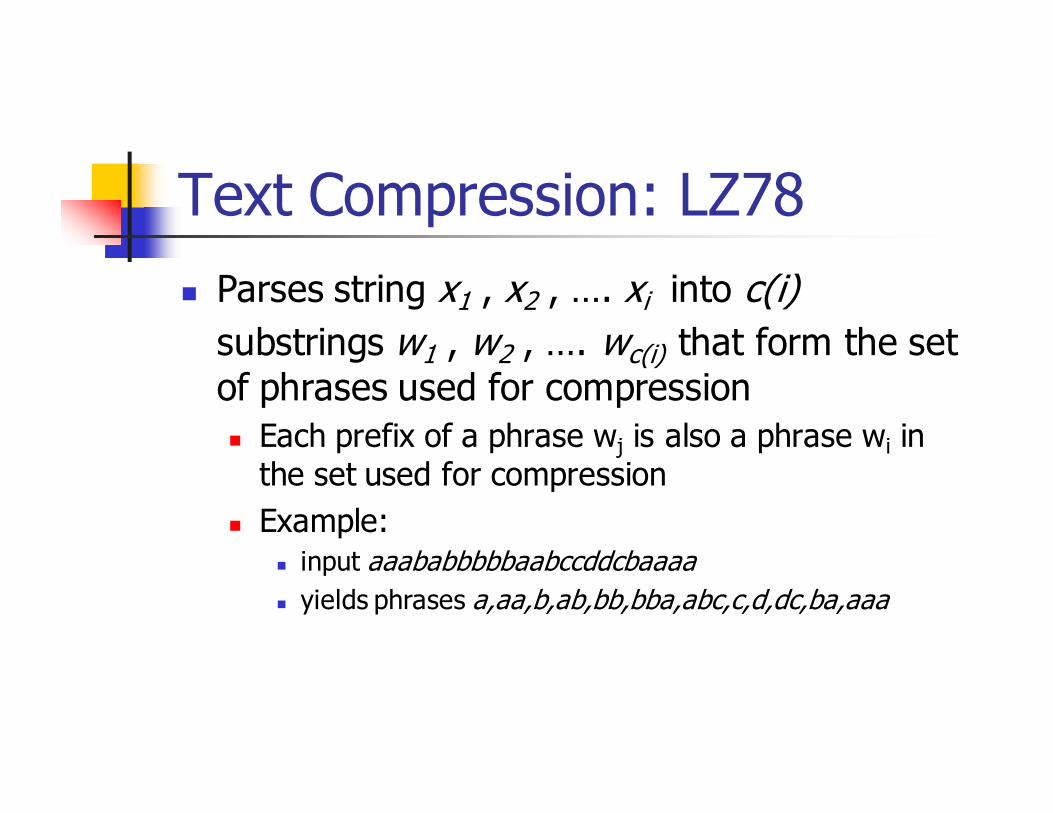
Text Compression: LZ78
� Parses string x1 , x2 , …. xi into c(i)
substrings w1 , w2 , …. wc(i) that form the set
of phrases used for compression
� Each prefix of a phrase wj is also a phrase wi in the set used for compression
� Example: � input aaababbbbbaabccddcbaaaa
� yields phrases a,aa,b,ab,bb,bba,abc,c,d,dc,ba,aaa
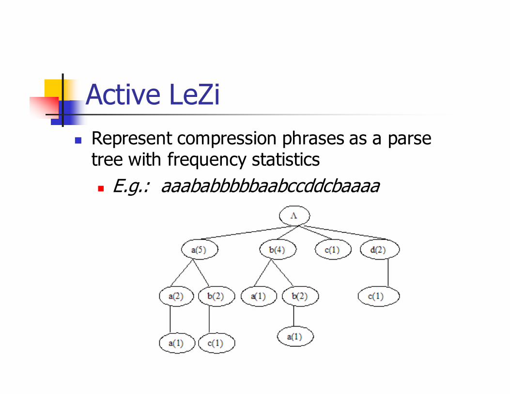
Active LeZi
� Represent compression phrases as a parse tree with frequency statistics
� E.g.: aaababbbbbaabccddcbaaaa

Prediction in Active LeZi
� Calculate the probability for each possible event� To calculate the probability, transitions across phrase boundaries have to be considered
� Slide window across the input sequence
� Length k equal to longest phrase seen so far
� Gather statistics on all possible contexts
� Order k-1 Markov model
� Output event with greatest probability across all contexts as prediction
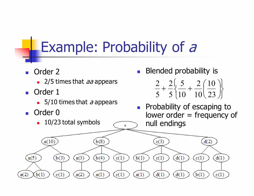
Example: Probability of a
� Order 2� 2/5 times that aa appears
� Order 1
� 5/10 times that a appears
� Order 0� 10/23 total symbols
� Blended probability is
� Probability of escaping to lower order = frequency of null endings
++23
10
10
2
10
5
5
2
5
2
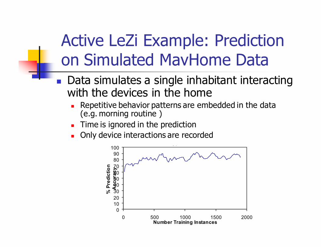
Active LeZi Example: Prediction on Simulated MavHome Data
ALZ Performance II - Typical Scenarios with noise
0
10
20
30
40
50
60
70
80
90
100
0 500 1000 1500 2000Number Training Instances
% Prediction
Accuracy
� Data simulates a single inhabitant interacting with the devices in the home� Repetitive behavior patterns are embedded in the data
(e.g. morning routine )
� Time is ignored in the prediction
� Only device interactions are recorded

Active LeZi
� Advantages
� Permits predictions based on sequence of events
� Does not require the construction of states
� Permits probabilistic predictions
� Problems
� Tree can become very large (long prediction times)
� Nonoptimal predictions if the tree is not sufficiently deep
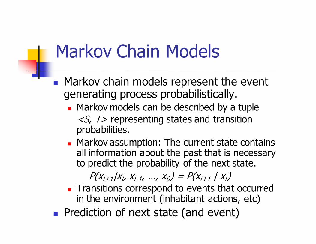
Markov Chain Models
� Markov chain models represent the event generating process probabilistically.� Markov models can be described by a tuple
<S, T> representing states and transition probabilities.
� Markov assumption: The current state contains all information about the past that is necessary to predict the probability of the next state.
P(xt+1|xt, xt-1, …, x0) = P(xt+1 | xt)
� Transitions correspond to events that occurred in the environment (inhabitant actions, etc)
� Prediction of next state (and event)

Markov Chain Example
� Example states: � S = {(Room, Time, Day, Previous Room)}
� Transition probabilities can be calculated from training data by counting occurrences
x1
x4
x6
x2
x5
x3
ocurredxtimesof
xfollowedxtimesofxxP
j
ji
ji#
#)|( =
Markov Models
� Advantages
� Permits probabilistic predictions
� Transition probabilities are easy to learn
� Representation is easy to interpret
� Problems
� State space has to have Markov property
� State space selection is not automatic
� States might have to include previous information
� State attributes might not be observable
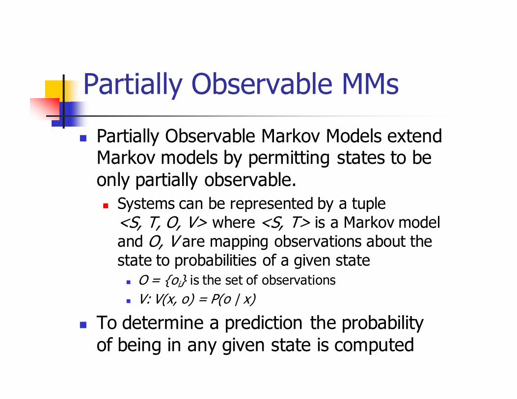
Partially Observable MMs
� Partially Observable Markov Models extend Markov models by permitting states to be
only partially observable.
� Systems can be represented by a tuple <S, T, O, V> where <S, T> is a Markov model and O, V are mapping observations about the state to probabilities of a given state
� O = {oi} is the set of observations
� V: V(x, o) = P(o | x)
� To determine a prediction the probability
of being in any given state is computed

Partially Observable MMs
� Prediction is the most likely next state given the information about the current state (i.e.
the current belief state):
� Belief state B is a probability distribution over the state space:
B = ((x1, P(x1)), …, (xn, P(xn))
� Prediction of the next state:
∑=+
jx
jij
tii
t xxPxPxoP
xP )|()()|(
)(1
α
∑=ji x
jijx
xxPxPx )|()(maxarg^

Hidden Markov Models
� Hidden Markov Models (HMM) provide mechanisms to learn the Markov Model
<S, T> underlying a POMM from the
sequence of observations.
� Baum-Welch algorithm learns transition and observation probabilities as well as the state space (only the number of states has to be given)
� Model learned is the one that is most likely to explain the observed training sequences
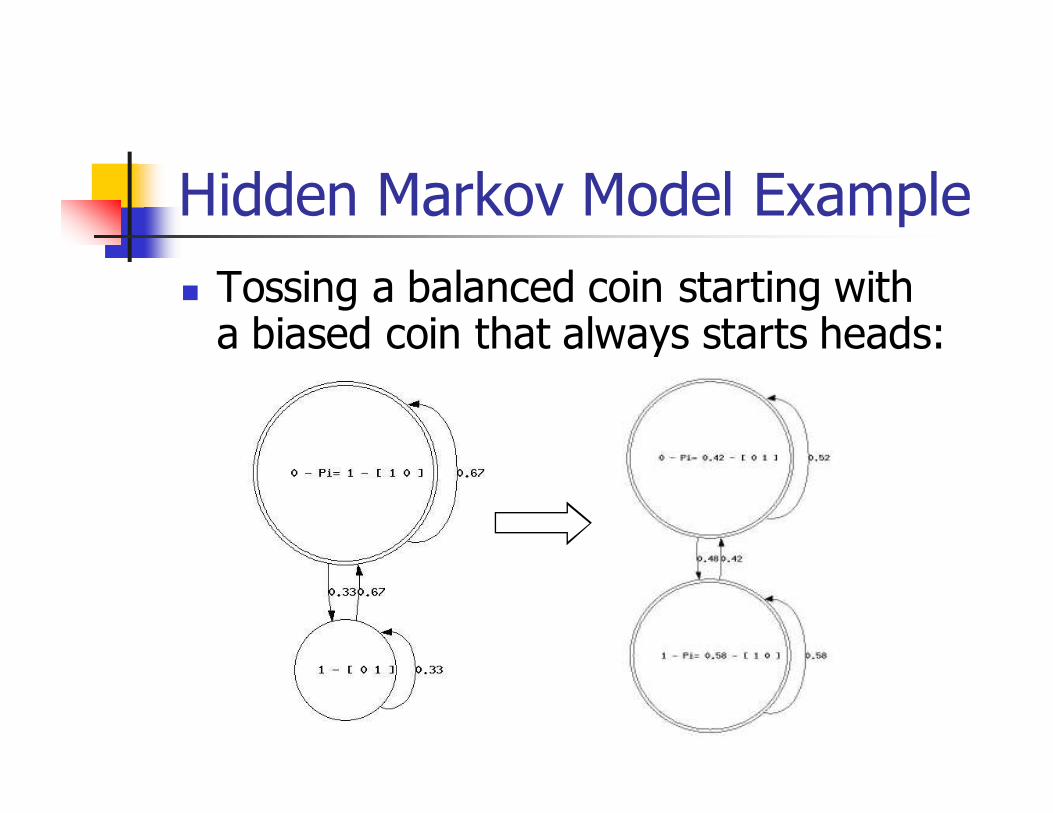
Hidden Markov Model Example
� Tossing a balanced coin starting with a biased coin that always starts heads:

Partially Observable MMs
� Advantages� Permits optimal predictions
� HMM provide algorithms to learn the model
� In HMM, Markovian state space description has not to be known
� Problems� State space can be enormous
� Learning of HMM is generally very complex
� Computation of belief state is computationally expensive
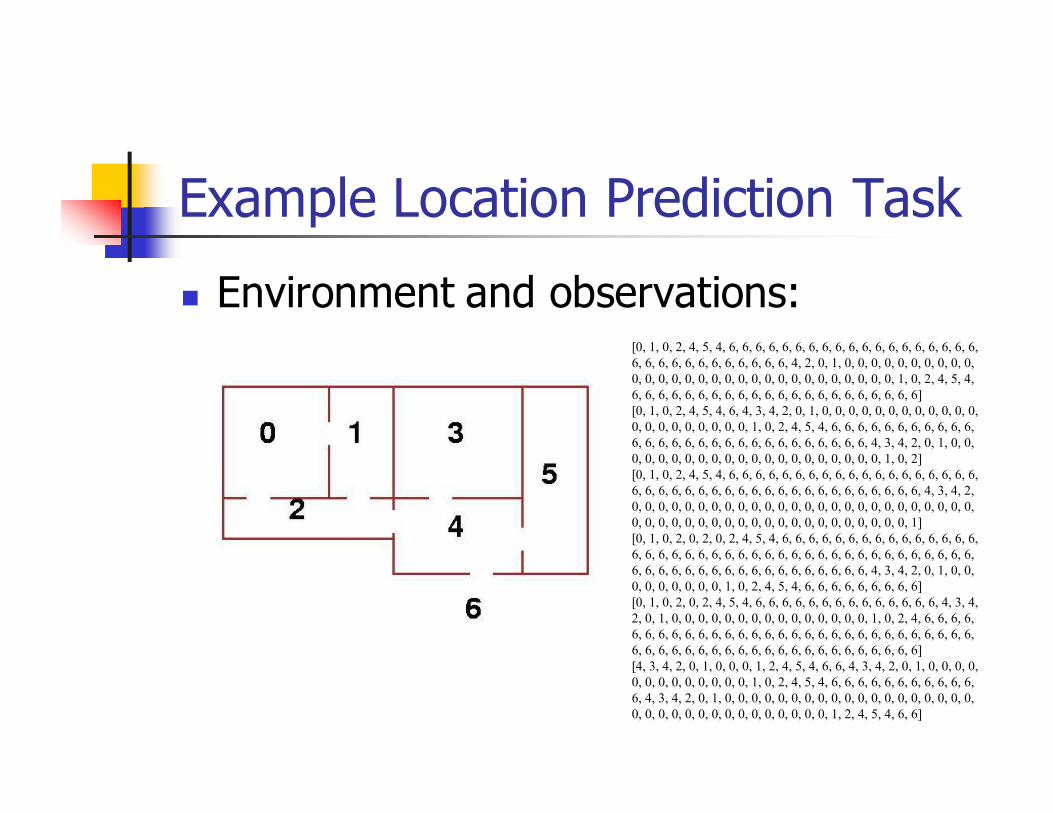
Example Location Prediction Task
� Environment and observations:[0, 1, 0, 2, 4, 5, 4, 6, 6, 6, 6, 6, 6, 6, 6, 6, 6, 6, 6, 6, 6, 6, 6, 6, 6, 6,
6, 6, 6, 6, 6, 6, 6, 6, 6, 6, 6, 6, 4, 2, 0, 1, 0, 0, 0, 0, 0, 0, 0, 0, 0, 0,
0, 0, 0, 0, 0, 0, 0, 0, 0, 0, 0, 0, 0, 0, 0, 0, 0, 0, 0, 0, 1, 0, 2, 4, 5, 4,
6, 6, 6, 6, 6, 6, 6, 6, 6, 6, 6, 6, 6, 6, 6, 6, 6, 6, 6, 6, 6, 6]
[0, 1, 0, 2, 4, 5, 4, 6, 4, 3, 4, 2, 0, 1, 0, 0, 0, 0, 0, 0, 0, 0, 0, 0, 0, 0,
0, 0, 0, 0, 0, 0, 0, 0, 0, 1, 0, 2, 4, 5, 4, 6, 6, 6, 6, 6, 6, 6, 6, 6, 6, 6,
6, 6, 6, 6, 6, 6, 6, 6, 6, 6, 6, 6, 6, 6, 6, 6, 6, 6, 4, 3, 4, 2, 0, 1, 0, 0,
0, 0, 0, 0, 0, 0, 0, 0, 0, 0, 0, 0, 0, 0, 0, 0, 0, 0, 0, 1, 0, 2]
[0, 1, 0, 2, 4, 5, 4, 6, 6, 6, 6, 6, 6, 6, 6, 6, 6, 6, 6, 6, 6, 6, 6, 6, 6, 6,
6, 6, 6, 6, 6, 6, 6, 6, 6, 6, 6, 6, 6, 6, 6, 6, 6, 6, 6, 6, 6, 6, 4, 3, 4, 2,
0, 0, 0, 0, 0, 0, 0, 0, 0, 0, 0, 0, 0, 0, 0, 0, 0, 0, 0, 0, 0, 0, 0, 0, 0, 0,
0, 0, 0, 0, 0, 0, 0, 0, 0, 0, 0, 0, 0, 0, 0, 0, 0, 0, 0, 0, 0, 1]
[0, 1, 0, 2, 0, 2, 0, 2, 4, 5, 4, 6, 6, 6, 6, 6, 6, 6, 6, 6, 6, 6, 6, 6, 6, 6,
6, 6, 6, 6, 6, 6, 6, 6, 6, 6, 6, 6, 6, 6, 6, 6, 6, 6, 6, 6, 6, 6, 6, 6, 6, 6,
6, 6, 6, 6, 6, 6, 6, 6, 6, 6, 6, 6, 6, 6, 6, 6, 6, 6, 4, 3, 4, 2, 0, 1, 0, 0,
0, 0, 0, 0, 0, 0, 0, 1, 0, 2, 4, 5, 4, 6, 6, 6, 6, 6, 6, 6, 6, 6]
[0, 1, 0, 2, 0, 2, 4, 5, 4, 6, 6, 6, 6, 6, 6, 6, 6, 6, 6, 6, 6, 6, 6, 4, 3, 4,
2, 0, 1, 0, 0, 0, 0, 0, 0, 0, 0, 0, 0, 0, 0, 0, 0, 0, 1, 0, 2, 4, 6, 6, 6, 6,
6, 6, 6, 6, 6, 6, 6, 6, 6, 6, 6, 6, 6, 6, 6, 6, 6, 6, 6, 6, 6, 6, 6, 6, 6, 6,
6, 6, 6, 6, 6, 6, 6, 6, 6, 6, 6, 6, 6, 6, 6, 6, 6, 6, 6, 6, 6, 6]
[4, 3, 4, 2, 0, 1, 0, 0, 0, 1, 2, 4, 5, 4, 6, 6, 4, 3, 4, 2, 0, 1, 0, 0, 0, 0,
0, 0, 0, 0, 0, 0, 0, 0, 0, 1, 0, 2, 4, 5, 4, 6, 6, 6, 6, 6, 6, 6, 6, 6, 6, 6,
6, 4, 3, 4, 2, 0, 1, 0, 0, 0, 0, 0, 0, 0, 0, 0, 0, 0, 0, 0, 0, 0, 0, 0, 0, 0,
0, 0, 0, 0, 0, 0, 0, 0, 0, 0, 0, 0, 0, 0, 0, 1, 2, 4, 5, 4, 6, 6]
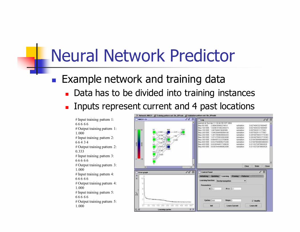
Neural Network Predictor
� Example network and training data
� Data has to be divided into training instances
� Inputs represent current and 4 past locations
# Input training pattern 1:
6 6 6 6 6
# Output training pattern 1:
1.000
# Input training pattern 2:
6 6 4 3 4
# Output training pattern 2:
0.333
# Input training pattern 3:
6 6 6 6 6
# Output training pattern 3:
1.000
# Input training pattern 4:
6 6 6 6 6
# Output training pattern 4:
1.000
# Input training pattern 5:
6 6 6 6 6
# Output training pattern 5:
1.000
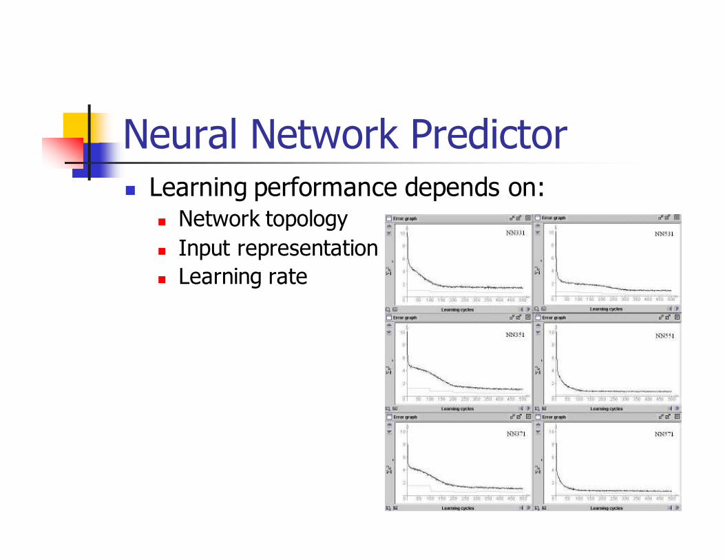
Neural Network Predictor � Learning performance depends on:
� Network topology
� Input representation
� Learning rate
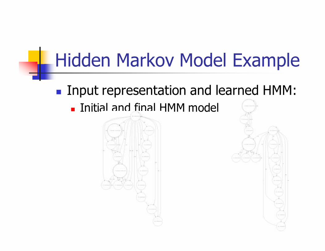
Hidden Markov Model Example
� Input representation and learned HMM:
� Initial and final HMM model
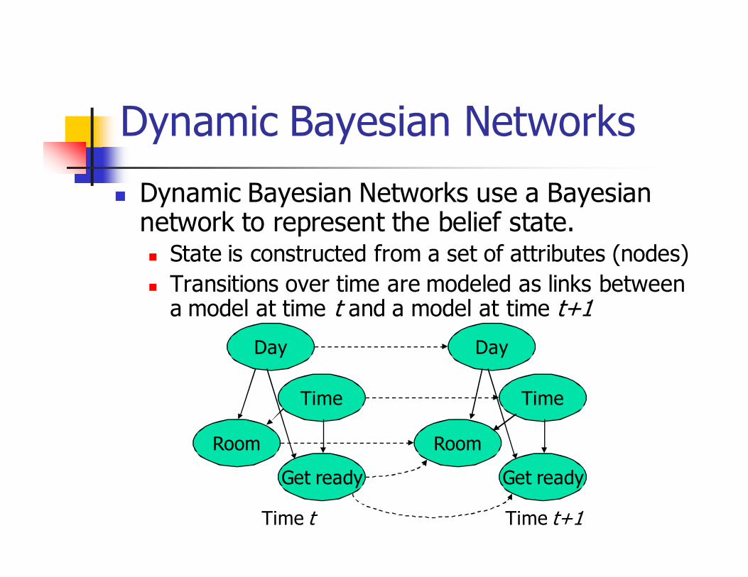
Dynamic Bayesian Networks
� Dynamic Bayesian Networks use a Bayesian network to represent the belief state.� State is constructed from a set of attributes (nodes)
� Transitions over time are modeled as links between a model at time t and a model at time t+1
Get ready
Time
Day
Room
Get ready
Time
Day
Room
Time t Time t+1

Dynamic Bayesian Networks
� Advantages
� Handles partial observability
� More compact model
� Belief state is inherent in the network
� Simple prediction of next belief state
� Problems
� State attributes have to be predetermined
� Learning of probabilities is very complex
Conclusions� Prediction is important in intelligent environments� Captures repetitive patterns (activities)
� Helps automating activities (But: only tells what will happen next; not what the system should do next)
� Different prediction algorithms have different strength and weaknesses:� Select a prediction approach that is suitable for the particular problem.
� There is no “best” prediction approach
� Optimal prediction is a very hard problem and is not yet solved.