Embed Size (px)
Citation preview

USING HYDRODESKTOP TO FIND
DATA FOR WATERSHED HYDROLOGY
Exercise 4
February 10, 2011
by:
Gonzalo E. Espinoza, Dr. Tim Whiteaker, and Dr. David Maidment Center for Research in Water Resources
The University of Texas at Austin
Table of Contents
Introduction ................................................................................................................................................................... 1
Installing HydroDesktop on Your Computer .............................................................................................................. 1
Using HydroDesktop through vDesk .......................................................................................................................... 2
Walkthrough: Downloading Data with HydroDesktop .................................................................................................. 4
Getting To Know the User Interface .......................................................................................................................... 4
Working with Projects ............................................................................................................................................... 5
Enabling Online Basemaps......................................................................................................................................... 6
Delineating Watersheds ............................................................................................................................................ 7
Searching for Hydrologic Data ................................................................................................................................... 9
Downloading Time Series ........................................................................................................................................ 13
Visualizing Time Series Data .................................................................................................................................... 14
Exporting Data ......................................................................................................................................................... 15
Exercise: Bull Creek ...................................................................................................................................................... 20
Exercise Procedure .................................................................................................................................................. 20
Items To Be Turned In .............................................................................................................................................. 22

1
INTRODUCTION
In Exercise 1, you solved Problem 2.3.2 from Applied Hydrology, in which you plotted the distribution of
precipitation, streamflow, and storage in a watershed using data supplied by the book. Now you will learn how to
obtain data for a different watershed using HydroDesktop, a free application for discovering, using, and managing
hydrologic time series data. HydroDesktop is designed to exploit the utility of WaterOneFlow Web services
developed by the Consortium of Universities for the Advancement of Hydrologic Science, Inc. (CUAHSI) Hydrologic
Information Systems project (CUAHSI-HIS). These services provide a standard access mechanism for hydrologic
data, which many organizations such as the United States Geological Survey are now using to publish their data.
Thus, through HydroDesktop, you have access to a vast wealth of freely available hydrologic data.
In this exercise, you will complete the same analysis as in Problem 2.3.2, but for the Bull Creek Watershed in Travis
County, Texas. You must use HydroDesktop to acquire the data for the exercise; therefore, you need to decide
how you want to run HydroDesktop. If you have a computer with a Windows operating system (e.g., XP, Vista, 7),
then you can install HydroDesktop and complete the exercise using your own computer. If you cannot (or do not
want to) install HydroDesktop on your computer, then you can use the school’s vDesk service, which gives you
remote access to a computer on which HydroDesktop is already installed. The steps for setting up both of these
options are provided in the following sections. Then, the procedure for completing the exercise is provided.
Related Links:
CUAHSI-HIS: http://his.cuahsi.org/
HydroDesktop: http://www.hydrodesktop.org
INSTALLING HYDRODESKTOP ON YOUR COMPUTER
If you have a computer with a Windows operating system, then you can download and install HydroDesktop on
that computer. HydroDesktop is still undergoing active development, and so new releases are published quite
frequently. For this exercise, please use version 1.1.390 of HydroDesktop. This version has been tested with the
exercise and should perform correctly.
To install version 1.1.390 of HydroDeskop:
1. In a Web browser, navigate to http://www.hydrodesktop.org (this redirects automatically to
http://hydrodesktop.codeplex.com/).
2. Click the Downloads tab near the top of the page (Figure 1).
3. In the list of Other Downloads on the right, click the link for 1.1.390. This takes you to the download page
for version 1.1.390.
4. Click the link for HydroDesktop_Installer_1.1.390.exe.
5. Read the license and agree to it.
6. Save and run the installer, accepting all defaults. The installer will guide you through the rest. Note for
Windows Vista or Windows 7 users: You may have to right-click the installer and click to Run as
administrator in order to run the installer.

2
Figure 1 You can choose which version of HydroDesktop to download through the Downloads tab
Once HydroDesktop is installed, please proceed to Walkthrough: Downloading Data with HydroDesktop.
USING HYDRODESKTOP THROUGH VDESK
If you will not be running HydroDesktop on your own computer, then you can use a service called vDesk to gain
remote access to a computer on which HydroDesktop is installed. If you have never used vDesk, then you must
first complete a one-time setup to install a vDesk client called VMware View Client. The steps to complete the
setup are outlined here, followed by the steps to access HydroDesktop through vDesk once the setup has been
completed.
Note
Using vDesk requires that your EID has been enabled for access to Cockrell School of Engineering resources. If
you’ve been using engineering computer labs, then you are probably fine. If you think you may need to enable
your EID, then please follow the instructions for doing so at http://www.engr.utexas.edu/itg/data/321-students.
To install VMware View Client:
1. In a Web browser, navigate to https://cse.vdesk.utexas.edu.
2. Click the View Client link that best matches your computer configuration. For example, if you are using Windows 7 64-bit, then you should download View Client (64-bit).
3. Save and run the installer. Note for Windows Vista or Windows 7 users: You may have to right-click the installer and click to Run as administrator in order to run the installer.
4. Accept all defaults and complete the installation. VMware View Client is now available as a program on your computer.
With VMware View Client installed, you can now log in to a remote computer that already has HydroDesktop
installed.
To access the remote computer through vDesk:
1. Start VMware View Client.
2. For the Connection Server, enter cse.vdesk.utexas.edu and click Connect.
3. Log in with your EID and password.
4. In the list of virtual desktops, select CSE – Lab – Common and click Connect.
3
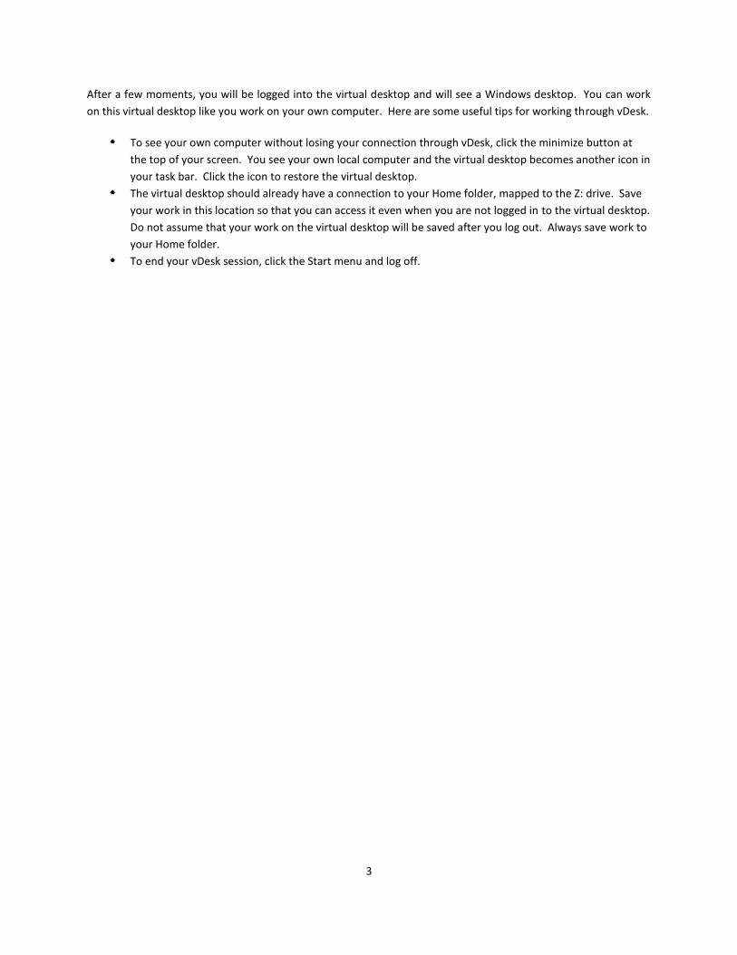
After a few moments, you will be logged into the virtual desktop and will see a Windows desktop. You can work
on this virtual desktop like you work on your own computer. Here are some useful tips for working through vDesk.
To see your own computer without losing your connection through vDesk, click the minimize button at
the top of your screen. You see your own local computer and the virtual desktop becomes another icon in
your task bar. Click the icon to restore the virtual desktop.
The virtual desktop should already have a connection to your Home folder, mapped to the Z: drive. Save
your work in this location so that you can access it even when you are not logged in to the virtual desktop.
Do not assume that your work on the virtual desktop will be saved after you log out. Always save work to
your Home folder.
To end your vDesk session, click the Start menu and log off.
4
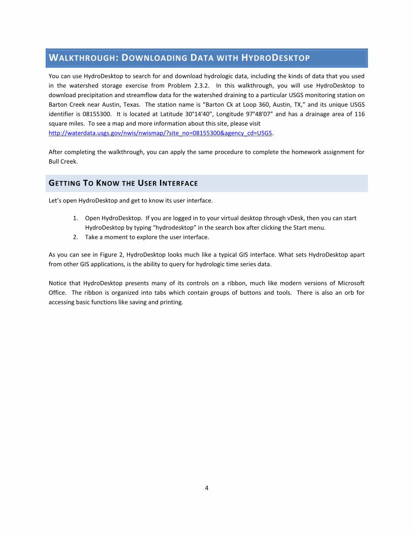
WALKTHROUGH: DOWNLOADING DATA WITH HYDRODESKTOP
You can use HydroDesktop to search for and download hydrologic data, including the kinds of data that you used
in the watershed storage exercise from Problem 2.3.2. In this walkthrough, you will use HydroDesktop to
download precipitation and streamflow data for the watershed draining to a particular USGS monitoring station on
Barton Creek near Austin, Texas. The station name is “Barton Ck at Loop 360, Austin, TX,” and its unique USGS
identifier is 08155300. It is located at Latitude 30°14'40", Longitude 97°48'07" and has a drainage area of 116
square miles. To see a map and more information about this site, please visit
http://waterdata.usgs.gov/nwis/nwismap/?site_no=08155300&agency_cd=USGS.
After completing the walkthrough, you can apply the same procedure to complete the homework assignment for
Bull Creek.
GETTING TO KNOW THE USER INTERFACE
Let’s open HydroDesktop and get to know its user interface.
1. Open HydroDesktop. If you are logged in to your virtual desktop through vDesk, then you can start
HydroDesktop by typing “hydrodesktop” in the search box after clicking the Start menu.
2. Take a moment to explore the user interface.
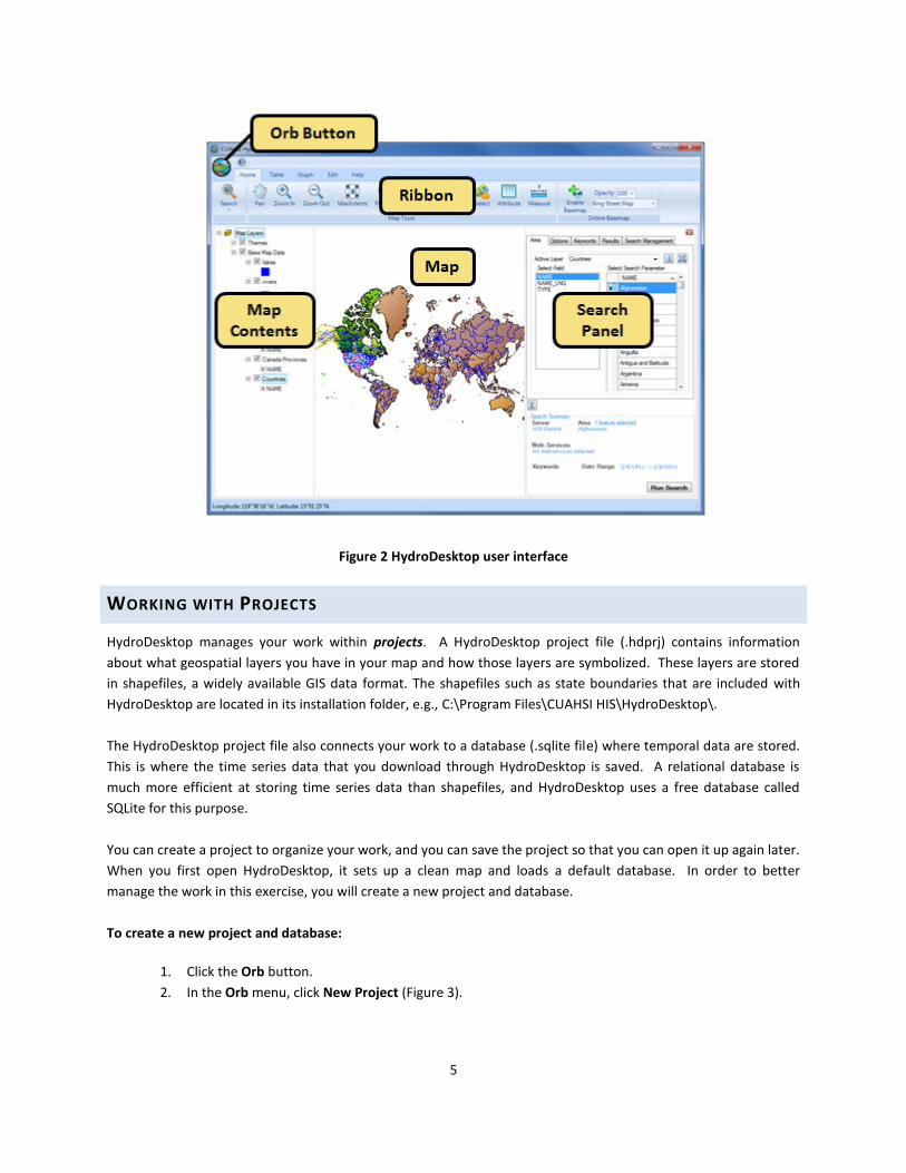
As you can see in Figure 2, HydroDesktop looks much like a typical GIS interface. What sets HydroDesktop apart
from other GIS applications, is the ability to query for hydrologic time series data.
Notice that HydroDesktop presents many of its controls on a ribbon, much like modern versions of Microsoft
Office. The ribbon is organized into tabs which contain groups of buttons and tools. There is also an orb for
accessing basic functions like saving and printing.
5
Figure 2 HydroDesktop user interface
WORKING WITH PROJECTS
HydroDesktop manages your work within projects. A HydroDesktop project file (.hdprj) contains information
about what geospatial layers you have in your map and how those layers are symbolized. These layers are stored
in shapefiles, a widely available GIS data format. The shapefiles such as state boundaries that are included with
HydroDesktop are located in its installation folder, e.g., C:\Program Files\CUAHSI HIS\HydroDesktop\.
The HydroDesktop project file also connects your work to a database (.sqlite file) where temporal data are stored.
This is where the time series data that you download through HydroDesktop is saved. A relational database is
much more efficient at storing time series data than shapefiles, and HydroDesktop uses a free database called
SQLite for this purpose.
You can create a project to organize your work, and you can save the project so that you can open it up again later.
When you first open HydroDesktop, it sets up a clean map and loads a default database. In order to better
manage the work in this exercise, you will create a new project and database.
To create a new project and database:
1. Click the Orb button.
2. In the Orb menu, click New Project (Figure 3).

6
Figure 3 Creating a new project
3. Choose a location to save your project such as your desktop. Users of vDesk should save their project
in their Home folder (on the Z: drive).
4. Name the project “WatershedHydrology” and then click Save.
HydroDesktop will notify you that the project was created successfully. The text in the title bar of the
HydroDesktop window should now include the name of your project. HydroDesktop has also created a database
for your project named WatershedHydrology.sqlilte. This database is saved in the same location as your project
file.
You are now ready to work within your newly created project and database. To save your project after performing
some work, click on the Save Project button in the Orb menu. To open a project, click on the Open Project button
in the Orb menu.
ENABLING ONLINE BASEMAPS
For a better sense of context, you can enable online basemaps from ESRI, Bing, and OpenStreetMap. These are
cartographically pleasing maps cached at multiple scales which are accessed in real time as you move around in
the HydroDesktop map. For this exercise, you will enable the ESRI Hydro Basemap. This map shows rivers and
watershed boundaries in the USA.
To enable the ESRI Hydro Basemap:
1. On the Home tab in the ribbon, find the Online Basemap group. Click the drop down list of basemaps
and choose ESRI Hydro Base Map.
2. Click Enable Basemap (Figure 4).
Figure 4 Enabling the Hydro Basemap
In addition to providing spatial context, you can see that this basemap can help you produce a more aesthetically
pleasing printed map.
7
DELINEATING WATERSHEDS
Since you’ll be downloading data pertinent to a particular watershed, it would be good to delineate the watershed
of interest. By using a Web service hosted by the EPA, HydroDesktop can delineate a watershed anywhere in the
continental United States without any local elevation data. All you have to do is click on the desired watershed
outlet location in the map, and then HydroDesktop sends that point location to the EPA service. The service
figures out which National Hydrography Dataset (NHD) reach the clicked point is closest to, and then finds all
catchments that the reach drains. The catchments are merged into a single watershed and returned to
HydroDesktop.
Note that the watershed returned is for the outlet of the entire reach, so if the point you clicked isn’t at the reach
outlet, then the resulting watershed will include some additional area downstream of your clicked point. Thus, this
tool is useful for helping to identify an area of interest but should not be used to determine watershed parameters
such as area. Future versions of the tool will support more precise delineation.
Let’s zoom to Barton Creek and delineate its watershed.
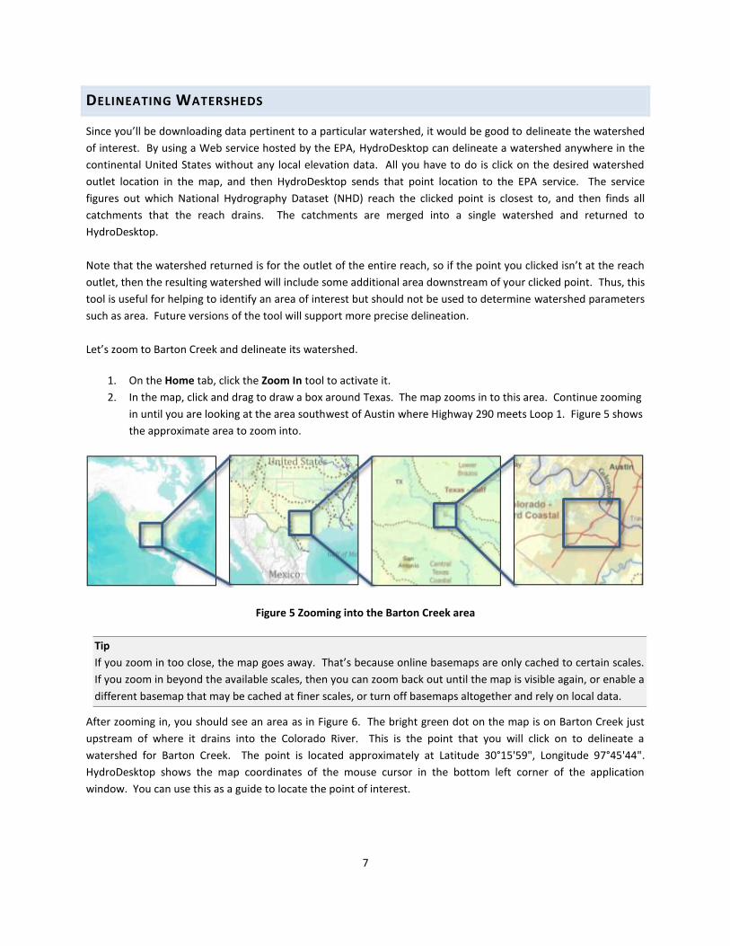
1. On the Home tab, click the Zoom In tool to activate it.
2. In the map, click and drag to draw a box around Texas. The map zooms in to this area. Continue zooming
in until you are looking at the area southwest of Austin where Highway 290 meets Loop 1. Figure 5 shows
the approximate area to zoom into.
Figure 5 Zooming into the Barton Creek area
Tip
If you zoom in too close, the map goes away. That’s because online basemaps are only cached to certain scales.
If you zoom in beyond the available scales, then you can zoom back out until the map is visible again, or enable a
different basemap that may be cached at finer scales, or turn off basemaps altogether and rely on local data.
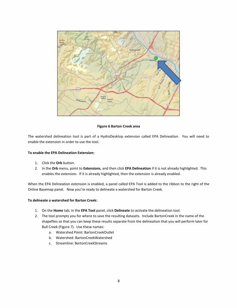
After zooming in, you should see an area as in Figure 6. The bright green dot on the map is on Barton Creek just
upstream of where it drains into the Colorado River. This is the point that you will click on to delineate a
watershed for Barton Creek. The point is located approximately at Latitude 30°15'59", Longitude 97°45'44".
HydroDesktop shows the map coordinates of the mouse cursor in the bottom left corner of the application
window. You can use this as a guide to locate the point of interest.
8
Figure 6 Barton Creek area
The watershed delineation tool is part of a HydroDesktop extension called EPA Delineation. You will need to
enable the extension in order to use the tool.
To enable the EPA Delineation Extension:
1. Click the Orb button.
2. In the Orb menu, point to Extensions, and then click EPA Delineation if it is not already highlighted. This
enables the extension. If it is already highlighted, then the extension is already enabled.
When the EPA Delineation extension is enabled, a panel called EPA Tool is added to the ribbon to the right of the
Online Basemap panel. Now you’re ready to delineate a watershed for Barton Creek.
To delineate a watershed for Barton Creek:
1. On the Home tab, in the EPA Tool panel, click Delineate to activate the delineation tool.
2. The tool prompts you for where to save the resulting datasets. Include BartonCreek in the name of the
shapefiles so that you can keep these results separate from the delineation that you will perform later for
Bull Creek (Figure 7). Use these names:
a. Watershed Point: BartonCreekOutlet
b. Watershed: BartonCreekWatershed
c. Streamline: BartonCreekStreams

9
Figure 7 Setting watershed filenames
3. Click on Barton Creek near its outlet. It doesn’t have to be exact, but try to click near where the green dot
is in Figure 6. Be careful not to click on the Colorado River (the large river flowing through Austin) or else
you will delineate a watershed for the wrong area.
After a moment, the watershed is shown in the map (highlighted in blue in Figure 8). The NHD reaches flowing to
the point that you clicked and the point itself are also shown.
Figure 8 Barton Creek Watershed
If you didn’t get the correct watershed delineated then you can activate the tool and try again. It’s OK to overwrite
previous results.
With the watershed delineated, now you’re ready to search for data in this watershed.
SEARCHING FOR HYDROLOGIC DATA
When searching for data in HydroDesktop, you can specify the following filters: region of interest, time period of
interest, data source and variables of interest. HydroDesktop then searches the CUAHSI-HIS national catalog of
known time series data to find locations of time series that match your search. Locations of time series data that
match your search are presented in the map. These results include information that HydroDesktop can use to
10
connect to each individual data provider for data access. You can further filter the results and then choose which
data you want to actually download and store in your database.
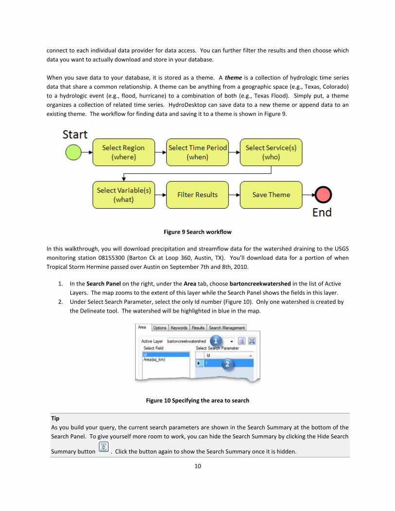
When you save data to your database, it is stored as a theme. A theme is a collection of hydrologic time series
data that share a common relationship. A theme can be anything from a geographic space (e.g., Texas, Colorado)
to a hydrologic event (e.g., flood, hurricane) to a combination of both (e.g., Texas Flood). Simply put, a theme
organizes a collection of related time series. HydroDesktop can save data to a new theme or append data to an
existing theme. The workflow for finding data and saving it to a theme is shown in Figure 9.
Figure 9 Search workflow
In this walkthrough, you will download precipitation and streamflow data for the watershed draining to the USGS
monitoring station 08155300 (Barton Ck at Loop 360, Austin, TX). You’ll download data for a portion of when
Tropical Storm Hermine passed over Austin on September 7th and 8th, 2010.
1. In the Search Panel on the right, under the Area tab, choose bartoncreekwatershed in the list of Active
Layers. The map zooms to the extent of this layer while the Search Panel shows the fields in this layer.
2. Under Select Search Parameter, select the only Id number (Figure 10). Only one watershed is created by
the Delineate tool. The watershed will be highlighted in blue in the map.
Figure 10 Specifying the area to search
Tip
As you build your query, the current search parameters are shown in the Search Summary at the bottom of the
Search Panel. To give yourself more room to work, you can hide the Search Summary by clicking the Hide Search
Summary button . Click the button again to show the Search Summary once it is hidden.

11
Next you will tell HydroDesktop the date range of time series that you want. For this exercise, you will choose the
period from 9/7/2010 to 9/9/2010.
3. In the Search Panel, click the Options tab to activate it.
4. Specify a Start Date of 9/7/2010 and an End Date of 9/9/2010 (Figure 11). You can click and type the
numbers in directly, or you can click the drop down arrow next to the date to open an interactive
calendar.
Now you will tell HydroDesktop from which data sources you want to query for data. You could search all data
sources, which is the default, but for this exercise we will use data from two specific Web services.
5. Click the Show Web Service Selection Panel checkbox.
6. Click Select None.
7. In the list of services, place a check next to Hermine Flood. This is a service that preserved USGS real-time
streamflow values during the Hermine storm for future study. Normally these values are not available
after 60 or 120 days from the date they were recorded.
8. In the list of services, place a check next to NWS-WGRFC USGS Water Region 12 Hourly MPE. This service
provides precipitation estimates based on NEXRAD radar rainfall data from the National Weather Service
West Gulf River Forecast Center.
Figure 11 Specifying a date range and data sources to search
With both data sources selected, you will now tell HydroDesktop what hydrologic variables you want to search for.
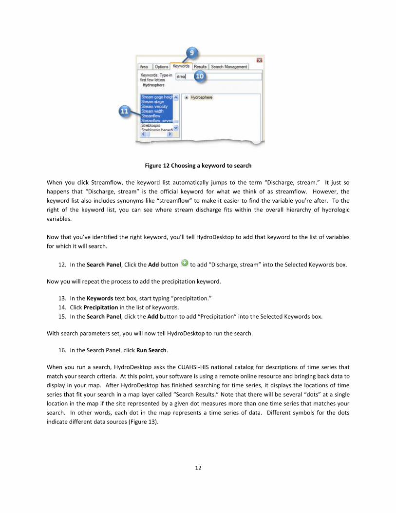
9. In the Search Panel, click the Keywords tab to activate it.
10. Start typing “streamflow” in the Keywords text box. The list of keywords automatically selects keywords
that match your search.
11. Click Streamflow in the list of keywords (Figure 12).
12
Figure 12 Choosing a keyword to search
When you click Streamflow, the keyword list automatically jumps to the term “Discharge, stream.” It just so
happens that “Discharge, stream” is the official keyword for what we think of as streamflow. However, the
keyword list also includes synonyms like “streamflow” to make it easier to find the variable you’re after. To the
right of the keyword list, you can see where stream discharge fits within the overall hierarchy of hydrologic
variables.
Now that you’ve identified the right keyword, you’ll tell HydroDesktop to add that keyword to the list of variables
for which it will search.
12. In the Search Panel, Click the Add button to add “Discharge, stream” into the Selected Keywords box.
Now you will repeat the process to add the precipitation keyword.
13. In the Keywords text box, start typing “precipitation.”
14. Click Precipitation in the list of keywords.
15. In the Search Panel, click the Add button to add “Precipitation” into the Selected Keywords box.
With search parameters set, you will now tell HydroDesktop to run the search.
16. In the Search Panel, click Run Search.
When you run a search, HydroDesktop asks the CUAHSI-HIS national catalog for descriptions of time series that
match your search criteria. At this point, your software is using a remote online resource and bringing back data to
display in your map. After HydroDesktop has finished searching for time series, it displays the locations of time
series that fit your search in a map layer called “Search Results.” Note that there will be several “dots” at a single
location in the map if the site represented by a given dot measures more than one time series that matches your
search. In other words, each dot in the map represents a time series of data. Different symbols for the dots
indicate different data sources (Figure 13).
13
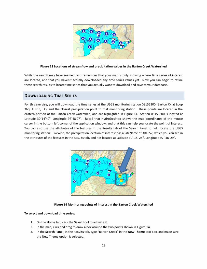
Figure 13 Locations of streamflow and precipitation values in the Barton Creek Watershed
While the search may have seemed fast, remember that your map is only showing where time series of interest
are located, and that you haven’t actually downloaded any time series values yet. Now you can begin to refine
these search results to locate time series that you actually want to download and save to your database.
DOWNLOADING TIME SERIES
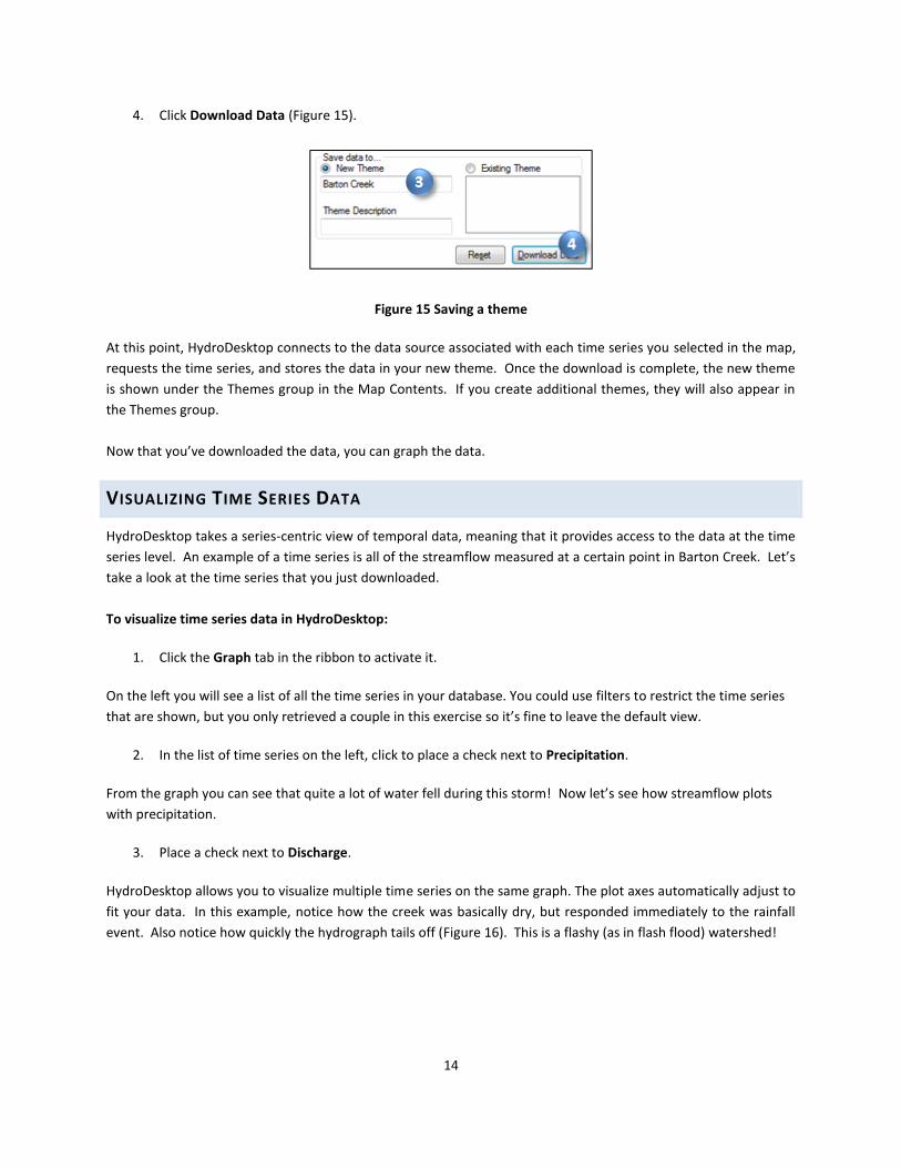
For this exercise, you will download the time series at the USGS monitoring station 08155300 (Barton Ck at Loop
360, Austin, TX), and the closest precipitation point to that monitoring station. These points are located in the
eastern portion of the Barton Creek watershed, and are highlighted in Figure 14. Station 08155300 is located at
Latitude 30°14'40", Longitude 97°48'07". Recall that HydroDesktop shows the map coordinates of the mouse
cursor in the bottom left corner of the application window, and that this can help you locate the point of interest.
You can also use the attributes of the features in the Results tab of the Search Panel to help locate the USGS
monitoring station. Likewise, the precipitation location of interest has a SiteName of 301657, which you can see in
the attributes of the features in the Results tab, and it is located at Latitude 30° 15' 28", Longitude 97° 48' 29".
Figure 14 Monitoring points of interest in the Barton Creek Watershed
To select and download time series:
1. On the Home tab, click the Select tool to activate it.
2. In the map, click and drag to draw a box around the two points shown in Figure 14.
3. In the Search Panel, in the Results tab, type “Barton Creek” in the New Theme text box, and make sure
the New Theme option is selected.
14
4. Click Download Data (Figure 15).
Figure 15 Saving a theme
At this point, HydroDesktop connects to the data source associated with each time series you selected in the map,
requests the time series, and stores the data in your new theme. Once the download is complete, the new theme
is shown under the Themes group in the Map Contents. If you create additional themes, they will also appear in
the Themes group.
Now that you’ve downloaded the data, you can graph the data.
VISUALIZING TIME SERIES DATA
HydroDesktop takes a series-centric view of temporal data, meaning that it provides access to the data at the time
series level. An example of a time series is all of the streamflow measured at a certain point in Barton Creek. Let’s
take a look at the time series that you just downloaded.
To visualize time series data in HydroDesktop:
1. Click the Graph tab in the ribbon to activate it.
On the left you will see a list of all the time series in your database. You could use filters to restrict the time series
that are shown, but you only retrieved a couple in this exercise so it’s fine to leave the default view.
2. In the list of time series on the left, click to place a check next to Precipitation.
From the graph you can see that quite a lot of water fell during this storm! Now let’s see how streamflow plots
with precipitation.
3. Place a check next to Discharge.
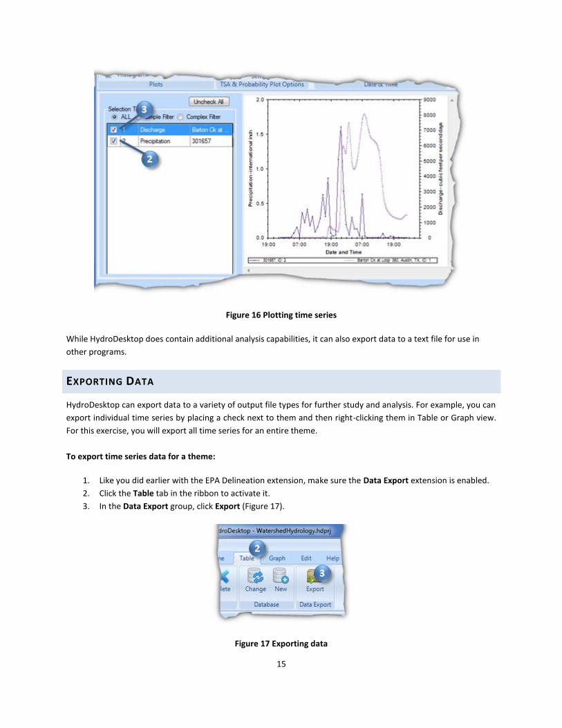
HydroDesktop allows you to visualize multiple time series on the same graph. The plot axes automatically adjust to
fit your data. In this example, notice how the creek was basically dry, but responded immediately to the rainfall
event. Also notice how quickly the hydrograph tails off (Figure 16). This is a flashy (as in flash flood) watershed!
15
Figure 16 Plotting time series
While HydroDesktop does contain additional analysis capabilities, it can also export data to a text file for use in
other programs.
EXPORTING DATA
HydroDesktop can export data to a variety of output file types for further study and analysis. For example, you can
export individual time series by placing a check next to them and then right-clicking them in Table or Graph view.
For this exercise, you will export all time series for an entire theme.
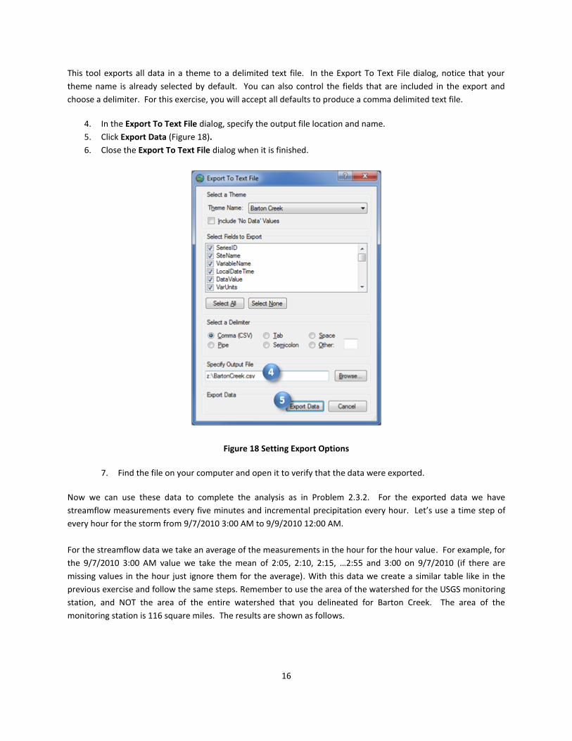
To export time series data for a theme:
1. Like you did earlier with the EPA Delineation extension, make sure the Data Export extension is enabled.
2. Click the Table tab in the ribbon to activate it.
3. In the Data Export group, click Export (Figure 17).
Figure 17 Exporting data
16
This tool exports all data in a theme to a delimited text file. In the Export To Text File dialog, notice that your
theme name is already selected by default. You can also control the fields that are included in the export and
choose a delimiter. For this exercise, you will accept all defaults to produce a comma delimited text file.
4. In the Export To Text File dialog, specify the output file location and name.
5. Click Export Data (Figure 18).
6. Close the Export To Text File dialog when it is finished.
Figure 18 Setting Export Options
7. Find the file on your computer and open it to verify that the data were exported.
Now we can use these data to complete the analysis as in Problem 2.3.2. For the exported data we have
streamflow measurements every five minutes and incremental precipitation every hour. Let’s use a time step of
every hour for the storm from 9/7/2010 3:00 AM to 9/9/2010 12:00 AM.
For the streamflow data we take an average of the measurements in the hour for the hour value. For example, for
the 9/7/2010 3:00 AM value we take the mean of 2:05, 2:10, 2:15, …2:55 and 3:00 on 9/7/2010 (if there are
missing values in the hour just ignore them for the average). With this data we create a similar table like in the
previous exercise and follow the same steps. Remember to use the area of the watershed for the USGS monitoring
station, and NOT the area of the entire watershed that you delineated for Barton Creek. The area of the
monitoring station is 116 square miles. The results are shown as follows.
17
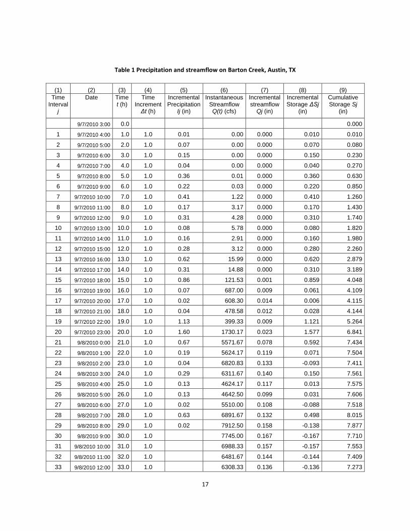
Table 1 Precipitation and streamflow on Barton Creek, Austin, TX
(1) (2) (3) (4) (5) (6) (7) (8) (9)
Time Interval
j
Date Time t (h)
Time Increment
Δt (h)
Incremental Precipitation
Ij (in)
Instantaneous Streamflow Q(t) (cfs)
Incremental streamflow
Qj (in)
Incremental Storage ΔSj
(in)
Cumulative Storage Sj
(in)
9/7/2010 3:00 0.0 0.000
1 9/7/2010 4:00 1.0 1.0 0.01 0.00 0.000 0.010 0.010
2 9/7/2010 5:00 2.0 1.0 0.07 0.00 0.000 0.070 0.080
3 9/7/2010 6:00 3.0 1.0 0.15 0.00 0.000 0.150 0.230
4 9/7/2010 7:00 4.0 1.0 0.04 0.00 0.000 0.040 0.270
5 9/7/2010 8:00 5.0 1.0 0.36 0.01 0.000 0.360 0.630
6 9/7/2010 9:00 6.0 1.0 0.22 0.03 0.000 0.220 0.850
7 9/7/2010 10:00 7.0 1.0 0.41 1.22 0.000 0.410 1.260
8 9/7/2010 11:00 8.0 1.0 0.17 3.17 0.000 0.170 1.430
9 9/7/2010 12:00 9.0 1.0 0.31 4.28 0.000 0.310 1.740
10 9/7/2010 13:00 10.0 1.0 0.08 5.78 0.000 0.080 1.820
11 9/7/2010 14:00 11.0 1.0 0.16 2.91 0.000 0.160 1.980
12 9/7/2010 15:00 12.0 1.0 0.28 3.12 0.000 0.280 2.260
13 9/7/2010 16:00 13.0 1.0 0.62 15.99 0.000 0.620 2.879
14 9/7/2010 17:00 14.0 1.0 0.31 14.88 0.000 0.310 3.189
15 9/7/2010 18:00 15.0 1.0 0.86 121.53 0.001 0.859 4.048
16 9/7/2010 19:00 16.0 1.0 0.07 687.00 0.009 0.061 4.109
17 9/7/2010 20:00 17.0 1.0 0.02 608.30 0.014 0.006 4.115
18 9/7/2010 21:00 18.0 1.0 0.04 478.58 0.012 0.028 4.144
19 9/7/2010 22:00 19.0 1.0 1.13 399.33 0.009 1.121 5.264
20 9/7/2010 23:00 20.0 1.0 1.60 1730.17 0.023 1.577 6.841
21 9/8/2010 0:00 21.0 1.0 0.67 5571.67 0.078 0.592 7.434
22 9/8/2010 1:00 22.0 1.0 0.19 5624.17 0.119 0.071 7.504
23 9/8/2010 2:00 23.0 1.0 0.04 6820.83 0.133 -0.093 7.411
24 9/8/2010 3:00 24.0 1.0 0.29 6311.67 0.140 0.150 7.561
25 9/8/2010 4:00 25.0 1.0 0.13 4624.17 0.117 0.013 7.575
26 9/8/2010 5:00 26.0 1.0 0.13 4642.50 0.099 0.031 7.606
27 9/8/2010 6:00 27.0 1.0 0.02 5510.00 0.108 -0.088 7.518
28 9/8/2010 7:00 28.0 1.0 0.63 6891.67 0.132 0.498 8.015
29 9/8/2010 8:00 29.0 1.0 0.02 7912.50 0.158 -0.138 7.877
30 9/8/2010 9:00 30.0 1.0 7745.00 0.167 -0.167 7.710
31 9/8/2010 10:00 31.0 1.0 6988.33 0.157 -0.157 7.553
32 9/8/2010 11:00 32.0 1.0 6481.67 0.144 -0.144 7.409
33 9/8/2010 12:00 33.0 1.0 6308.33 0.136 -0.136 7.273

18
34 9/8/2010 13:00 34.0 1.0 6091.67 0.132 -0.132 7.141
35 9/8/2010 14:00 35.0 1.0 5505.83 0.124 -0.124 7.017
36 9/8/2010 15:00 36.0 1.0 0.06 3900.91 0.100 -0.040 6.977
37 9/8/2010 16:00 37.0 1.0 2420.00 0.067 -0.067 6.909
38 9/8/2010 17:00 38.0 1.0 1821.67 0.045 -0.045 6.864
39 9/8/2010 18:00 39.0 1.0 0.02 1560.00 0.036 -0.016 6.848
40 9/8/2010 19:00 40.0 1.0 0.01 1390.83 0.031 -0.021 6.826
41 9/8/2010 20:00 41.0 1.0 1306.67 0.029 -0.029 6.798
42 9/8/2010 21:00 42.0 1.0 1237.50 0.027 -0.027 6.771
43 9/8/2010 22:00 43.0 1.0 1200.83 0.026 -0.026 6.745
44 9/8/2010 23:00 44.0 1.0 1268.33 0.026 -0.026 6.718
45 9/9/2010 0:00 45.0 1.0 1438.33 0.029 -0.029 6.689
Total 9.12 2.43
Figure 19 Precipitation and streamflow on Barton Creek, Austin, TX
Figure 20 Change in storage on Barton Creek, Austin, TX
0.00
0.20
0.40
0.60
0.80
1.00
1.20
1.40
1.60
1.80
1 3 5 7 9 11 13 15 17 19 21 23 25 27 29 31 33 35 37 39 41 43 45
Incr
em
en
tal D
ep
th (
in)
Time (h)
Precipitation Input Ij
Streamflow Output Qj
-0.500
0.000
0.500
1.000
1.500
2.000
1 3 5 7 9 11 13 15 17 19 21 23 25 27 29 31 33 35 37 39 41 43 45
Incr
em
en
tal D
ep
th (
in)
Time (h)
ΔSj = Ij - Qj Gain
Loss
19
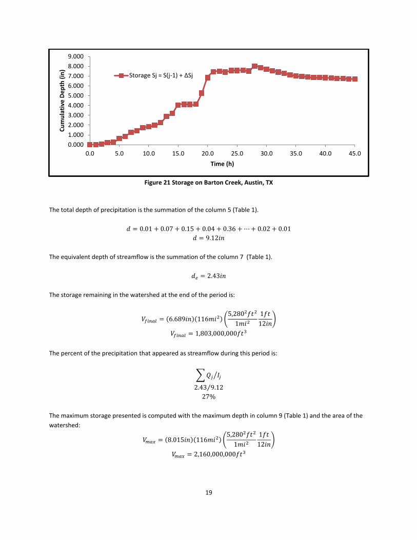
Figure 21 Storage on Barton Creek, Austin, TX
The total depth of precipitation is the summation of the column 5 (Table 1).
The equivalent depth of streamflow is the summation of the column 7 (Table 1).
The storage remaining in the watershed at the end of the period is:
( )( ) (
)
The percent of the precipitation that appeared as streamflow during this period is:
∑ ⁄
⁄
The maximum storage presented is computed with the maximum depth in column 9 (Table 1) and the area of the
watershed:
( )( ) (
)
0.000
1.000
2.000
3.000
4.000
5.000
6.000
7.000
8.000
9.000
0.0 5.0 10.0 15.0 20.0 25.0 30.0 35.0 40.0 45.0
Cu
mu
lati
ve D
ep
th (
in)
Time (h)
Storage Sj = S(j-1) + ΔSj
20
EXERCISE: BULL CREEK
Using the above walkthrough as a guide, complete the same procedure for the monitoring station on Bull Creek at
Highway 360 near Austin, Texas, for Tropical Storm Hermine from 9/7/2010 4:00:00 AM to 9/9/2010 12:00:00 AM.
Calculate the time distribution of storage on the watershed assuming that the initial storage is zero. Compute the
total depth of precipitation and the equivalent depth of streamflow which occurred during the period. How much
storage remained in the watershed at the end of the period? What percent of the precipitation appeared as
streamflow during this period? What was the maximum storage? Plot the time distribution of incremental
precipitation, streamflow, change in storage, and cumulative storage.
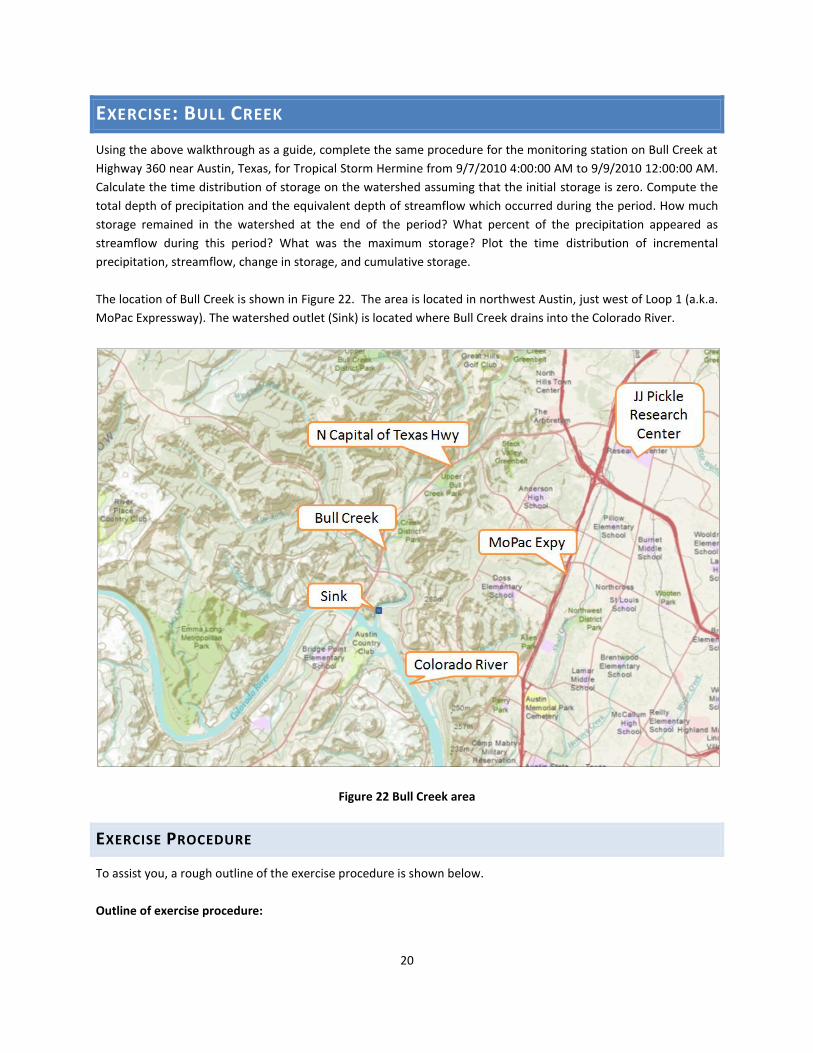
The location of Bull Creek is shown in Figure 22. The area is located in northwest Austin, just west of Loop 1 (a.k.a.
MoPac Expressway). The watershed outlet (Sink) is located where Bull Creek drains into the Colorado River.
Figure 22 Bull Creek area
EXERCISE PROCEDURE
To assist you, a rough outline of the exercise procedure is shown below.
Outline of exercise procedure:

21
1. On the Home tab, use the Map Tools to pan and zoom to the Bull Creek area as in Figure 22.
2. Activate the Delineate tool.
3. Specify these filenames:
a. Watershed Point: BullCreekOutlet
b. Watershed: BullCreekWatershed
c. Streamline: BullCreekStreams
4. Click on the point labeled “Sink” in Figure 22. The point is located approximately at Latitude 30°20'58",
Longitude 97°47'29". A watershed for Bull Creek is delineated.
As a hint, the resulting watershed for Bull Creek should look like the one highlighted in Figure 23.
Figure 23 Bull Creek Watershed
5. In the Search Panel, specify this search:
a. Area
i. Active Layer: bullcreekwatershed
ii. Select the record with Id = 1 (the only record available).
b. Options and Keywords – These should still be set from the previous search. You’ll use the same
parameters as in the previous search, so you can leave these as they are.
6. Click Run Search.
7. From the search results select these two sites located at the southern end of the watershed (Figure 24).
a. HermineFlood - Bull Ck at Loop 360 nr Austin, TX – 08154700 – Latitude 30°22'19", Longitude
97°47'04"
b. USGS_Region12_Hourly_MPE – 306760 – Latitude 30° 21' 39", Longitude 97° 47' 35"

22
Figure 24 Monitoring points of interest in the Bull Creek Watershed
8. Download the time series to a new theme called Bull Creek.
9. Plots graphs of the time series to visually check that the data were actually downloaded.
10. On the Table tab, click Export.
11. Choose Bull Creek as the Theme Name.
12. Specify a filename and export the data for the Bull Creek theme.
13. With the exported file and a program such as Excel, continue with the watershed storage analysis as in
Problem 2.3.2.
Remember to use the drainage area for the Bull Creek monitoring station and NOT the area for the entire Bull
Creek Watershed. The Bull Creek monitoring station is described at the link below:
http://waterdata.usgs.gov/nwis/nwismap/?site_no=08154700&agency_cd=USGS
From that link, the drainage area for the monitoring station is 22.3 square miles.
Complete the exercise for the time period from 9/7/2010 4:00:00 AM to 9/9/2010 12:00:00 AM.
ITEMS TO BE TURNED IN
Here is a list of items to be turned for the watershed storage analysis. These items apply to Bull Creek.
Solution of the Bull Creek Exercise
o Screen capture of a map of the Austin area with the watersheds for Bull Creek and Barton Creek
shown in it
o Precipitation and streamflow (table)
o Total depth of precipitation in inches
o Equivalent depth of streamflow which occurred in the period in inches
o Time Distribution: Precipitation and Streamflow Graph

23
o Time Distribution: Change in Storage Graph
o Time Distribution: Storage Graph
o Storage remaining in the watershed in cubic feet
o Percentage of precipitation appearing as streamflow in the period
o Maximum storage in cubic feet
Make a comparison between Barton Creek and Bull creek
Tip
For instructions on how to take screenshots in Windows, please visit:
http://www.wikihow.com/Take-a-Screenshot-in-Microsoft-Windows


![University of Texas at The University of Texas at … · [1] Maymester 2009 The University of Texas at Austin Photo: University of Texas at Austin School of Social Work professor](https://img.dokumen.tips/doc/110x75/5b8153fe7f8b9a2b678c1fff/university-of-texas-at-the-university-of-texas-at-1-maymester-2009-the-university.jpg)