Journal of Service Science and Management, 2014, 7, 277-290 Published Online August 2014 in SciRes. http://www.scirp.org/journal/jssm http://dx.doi.org/10.4236/jssm.2014.74025

How to cite this paper: Paradi, J.C., Wilson, D. and Yang, X.P. (2014) Data Envelopment Analysis of Corporate Failure for Non-Manufacturing Firms Using a Slacks-Based Measure. Journal of Service Science and Management, 7, 277-290. http://dx.doi.org/10.4236/jssm.2014.74025

Data Envelopment Analysis of Corporate Failure for Non-Manufacturing Firms Using a Slacks-Based Measure Joseph C. Paradi, D’Andre Wilson, Xiaopeng Yang* Centre for Management of Technology and Entrepreneurship, University of Toronto, Toronto, Canada Email: *Xiaopeng.yang@utoronto.ca Received 27 June 2014; revised 25 July 2014; accepted 16 August 2014

Copyright © 2014 by authors and Scientific Research Publishing Inc. This work is licensed under the Creative Commons Attribution International License (CC BY). http://creativecommons.org/licenses/by/4.0/

Abstract The problem of predicting corporate failure has intrigued many in the investment sector, corpo-rate decision makers, business partners and many others, hence the intense research efforts by industry and academia. The majority of former research efforts on this topic focused on manufac-turing companies with considerable assets commensurate with their size. But there is a dearth of publications on predicting non-manufacturing firms’ financial difficulties since these firms typi-cally do not have significant assets that rely heavily on assets, and a key variable cannot be ade-quate. Recently, data envelopment analysis (DEA) rather than Altman’s Z score model and tradi-tional parametric methods has become a research interest in predicting corporate failure. How-ever, there is still no research showing how to fix appropriate cut-off points to distinguish the performance of firms. Our research utilizes slack-based measure (SBM) DEA model to generate ef-ficiency scores for non-manufacturing firms; then we categorize these firms into safe, grey and distress zones by proposing cut-off points based on 5 years DEA analysis. The result shows that the proposed method has obvious advantages in predicting corporate financial stress.

Keywords Corporate Failure, Non-Manufacturing Company, Services Industry, Predictions, Data Envelopment Analysis (DEA), Altman’s Z Score

1. Introduction From the viewpoint of company management and individual investors, corporate health of a company is of critical importance as the firm’s future is in the balance. A very valuable piece of information would be the

*Corresponding author.

J. C. Paradi et al.

278

knowledge that if a profit organisation is headed for corporate financial stress or failure. There are various methods used to predict corporate failure before actual financial stress; one of the most

prevalent methods is to use financial ratios. In the past, a number of studies have been done using the informa-tion from financial statements, particularly financial ratios to predict corporate failure [1]. A prominent method of predicting bankruptcy is the Altman Z score [2]. Altman used Multiple Discriminant Analysis to create a model that used basic financial ratios in a linear formula to give a score. This score is used to classify a company into one of the following three categories: at the risk of corporate stress or failure, healthy, and the middle status, a “grey area”. The problem with these methods is that they were generalized for manufacturing firms, i.e. there was a major emphasis on the asset size of the firms involved [3] [4]. In recent times, more companies are non- manufacturing and service-oriented firms and thus have less focus on the overall asset-size of the company [5].

As a supplement to his original model, Altman created another model that he named the Altman Z'' model [6] to cover the non-manufacturing sector. Then he tested Z'' score on non-manufacturing firms and developed cor-responding coefficients to make his original model suitable for companies including both manufacturing and non-manufacturing companies. Nevertheless, this model is still substantially based on asset size notwithstanding the fact that a large number of companies are mainly focused on service and their most important asset is their people and they do not have a large real asset base [5]. It follows that an investigation of the Altman Z'' model for the non-manufacturing sector is necessary and this is proposed in this study.

DEA is a prevalent non-parametric approach in evaluating the relative efficiencies of a group of peer units, i.e. Decision Making Units (DMUs). The first DEA model, CCR, was first proposed in 1978 by Charnes et al. [7] who extended Farrell’s [8] prototype model about technical and allocative efficiency. Consequently, DEA de-veloped into a powerful tool which was applicable to a broad spectrum of research domains including manage-ment, finance, agriculture, non-profit organizations etc. [9]-[12].

There are two main benefits to use DEA in predicting corporate failure for non-manufacturing firms. One is that analysts could select inputs and outputs flexibly depending on their actual needs, which allow us to elimi-nate the “asset” factor for non-manufacturing firms. Another one is that DEA is a nonparametric method. Al-though parametric methodologies are widely used and offer desirable characteristics, they require prior parame-ter specifications (as does the Altman Z'' model), which are rather complicated for ordinary users. It follows that if we can eliminate asset, or at least significantly reduce its influence, when selecting inputs and outputs for the non-manufacturing company we could use the DEA score as a predictor of corporate financial health.

The remainder of this article is structured as follows: Section 2 reviews the previous methods in predicting corporate failure. Section 3 provides a detailed description of the SBM model which we employ in the specific application. Section 4 is an application of this approach to a real database, and we report the comparisons be-tween the Altman Z'' model and our SBM model. To conclude, Section 5 summarizes the research and provides additional discussion.

2. Literature Review Having a thorough understanding of the former studies related to bankruptcy prediction is essential if we are to make a valuable contribution to the existing knowledge of corporate failure prediction methods. This section outlines some of the most relevant and influential models and applications in bankruptcy prediction and reviews the details of these findings.

2.1. Parametric Methods One of the first attempts to predict insolvency or bankruptcy was carried out by William Beaver in 1967 [1]. Beaver defined failure as “the inability of a firm to pay its financial obligations as they mature” and a financial ratio as “a quotient of two numbers, where both numbers consist of financial statement items”. He also intro-duced a third term “predictive ability” which is essentially the usefulness of a data item in identifying an event before it occurs [1]. Beaver collected data from Moody’s industrial manual between 1954 and 1964, inclusive. Each failed firm from Moody’s was compared to a healthy firm in the same industry of a comparable asset size. At the time there were statistics based reasons to believe that the larger of two firms will have less probability of failure even if they have identical financial ratios. Therefore he believed that firms of different asset-sizes could not be accurately compared [13]. Beaver compiled 30 ratios and showed 14 to be the most effective, and then Beaver’s results ultimately showed “cash flow/total debt” as the best predictor, and “total debt/total assets” as

J. C. Paradi et al.

279

the second best. He noted that “the most crucial factor was the net liquid asset flow supplied to the reservoir while the size of the reservoir was the least important factor”.

Since Beaver’s univariate only selects the most crucial factor in failure analysis, but this is not objective or comprehensive. In 1968, Edward Altman attempted the first multivariate approach to bankruptcy prediction, which was named Multiple Discriminant Analysis (MDA) [2]. To develop the model Altman took a sample of 66 corporations with 33 firms in the bankrupt group and 33 in the non-bankrupt group [6]. A list of 22 potential ratios was compiled which were split into five standard ratio categories: liquidity, profitability, leverage, sol-vency and activity ratios. From the list of 22, five ratios were selected to be able to do the best overall job at collectively predicting bankruptcy. These were selected based on: 1) statistical significance of various potential functions while determining the relative contribution of each individual variable, 2) the inter-correlation be-tween the variables, 3) the predictive accuracy of various profiles and 4) judgement of the analysis [2]. Then Altman’s multivariate model is as follows:

1 2 3 4 51.2 1.4 3.3 0.6 0.999Z T T T T T= + + + + (1)

where

1working capital

total assetsT = , 2

retained earningstotal assets

T = , 3earnings before income & taxes

total assetsT = ,

4market value of equity

total liabilitiesT = , 5

salestotal assets

T = .

Altman also stated in his research that companies could be categorized into three zones by selected cut-off points, i.e. safe (Z > 2.6), grey (1.1 < Z < 2.6) and distress (Z < 1.1).

Based on Altman’s Z score method, a large number of related studies were developed by employing different ratios [14]-[21], of which the majority still focused on manufacturing companies. It follows that Altman pro-posed his lesser known Z'' score method which mainly dealt with the non-manufacturing industry as follows:

1 2 3 46.56 3.26 6.72 1.05Z T T T T′′ ′′ ′′ ′′ ′′= + + + (2)

where

1working capital

total assetsT ′′= , 2

retained earningstotal assets

T ′′= ,

3earnings before income & taxes

total assetsT ′′= , 4

book value of equitytotal liabilities

T ′′= .

Altman revised the coefficients and items in the former Z score model to form a Z'' score model. Even though the Z'' score model is called the attempt to examine alternative industries compared with the former Z score model, it still has a major influence by the firms’ asset size. Given this, a non-parametric method, i.e. DEA which is flexible in attribute selection is considered in this research.

2.2. Corporate Failure Prediction by DEA Recently, DEA becomes a welcome method in corporate failure prediction by comparing with various tradi-tional methods [22]-[25]. Cielen et al. compared linear programming model, decision tree method and DEA from the methodological aspect in corporate failure prediction, and concluded that there were no large accuracy discrepancies between linear programming model and DEA, but both methods outperformed decision tree method [26]. On the other hand, Sueyoshi et al. applied DEA-DA (discriminant analysis) into bankruptcy as-sessment by comparing to DEA method, and found out that DEA-DA is more appropriate for data set over time [27]. Furthermore, a novel DEA method integrating with rough set theory (RST) and support vector machines (SVM) was used to increase the accuracy of predicting corporate failure [28]. These studies utilized different methods to compare to DEA emphasizing the predominance of DEA in corporate failure prediction. However, as aforementioned, none of the studies focuses on the failure prediction for non-manufacturing firms which have a small asset size compared to other industries, and deserve more concentration.

Another shortcoming of these studies is that most of them emphasize the advantage of DEA as a non-para- metric efficiency evaluation tool unilaterally, but without enough explanation about how to use the efficiency

J. C. Paradi et al.

280

score generated by DEA models. In other words, there is no effective method to clarify the cut-off points of DEA scores which can indicate the performance of the firms. This research collected data for up to 5 years be-fore the bankruptcy of a firm. By analyzing the DEA scores, we divide the companies into safe, grey and dis-tress zones. Therefore, such a categorizing method would be more helpful for corporate management.

3. Methodology Since the basic constant returns to scale CCR model [7], DEA models’ capabilities have been significantly ex-tended to a broad approach, including both radial and non-radial models. While each DEA model has its uses, the CCR and BCC [29] models are limited by the fact that they do not account for mix inefficiencies. In this case, the company under examination is not limited to “proportional attributes change”, but is evaluated by the general deviation from best firms. It follows that the SBM model [30], which accounts for mix inefficiencies is more suitable for the current study.

3.1. Slacks-Based Measure We begin this section with a brief introduction to the SBM model. Suppose that a set of n DMUs of which input and output vectors are represented by an (m × n) matrix X and a (s × n) output matrix Y respectively. The num-ber of inputs and outputs are denoted by m and s. Thus the efficiency score of DMUo (the current DMU under examination) is formulated by the following fractional programming form of the SBM model.

1

, ,

1

11min 11

. .

0, 0, 0

mi

i ios

r

r ro

o

o

sm x

ss y

s t

ρ−

−

=+

=

−

−

−=

+

− =

+ =

≥ ≥ ≥

∑

∑+λ s s

+

+

x s Xλ

y s Yλ

λ s s

(3)

in which input and output vectors of DMUo are defined by ( )T1 2, , ,o o o mox x x=x and ( )T

1 2, , ,o o o soy y y=y . Slack vectors − ∈ ms R and + ∈ ss R are explained as input excesses and output shortfalls. The production possibility set P is defined as follows.

( ){ }, , , 0= ≥ ≤ ≥P x y x Xλ y Yλ λ (4)

It can thus be concluded that the combination (Xλ, Yλ) formed by a non-negative vector λ outperforms (xo, yo). Tone [30] stated that the above SBM model satisfied the following four properties: (P1) Units Invariance: The optimal value of the objective function is independent of the units in which the inputs and outputs are measured. (P2) Monotony: The efficiency of a DMU is monotonically decreasing along with the increase in each slack to either input or output. (P3) Reference Set Dependence: The efficiency of a DMU should be measured only by consulting its corresponding reference set. (P4) Charnes-Cooper Transformation: The above original nonlinear SBM model in (1) can be transformed into a linear one using the Charnes-Cooper transformation.

The objective function in (1) is interpreted as the ratio of the mean input and output mix inefficiencies with an upper limit of 1. Assume that the optimal solution of an inefficient DMUo by (1) is denoted as (ρ*, λ*, s−*, s+*), thus DMUo can be improved to be efficient by reducing its input excesses and augmenting its output shortfalls as follows:

*

*

ˆ

ˆo o

o o

−= −

= + +

x x s

y y s (5)

The new DMU ( )ˆ ˆ,o ox y defined by projecting DMUo to a given point on the efficiency frontier is usually considered to be an improving target. The reference set of DMUo, is constituted by all the positive elements in vector λ*. In the cases where only the slacks in the inputs are necessary to investigate, the input-oriented SBM model is usually utilized. The input-oriented SBM model actually is the numerator of the SBM model with cor-

J. C. Paradi et al.

281

responding proper modification to constraints that can be expressed as follows:

, , 1

11min

. .

0, 0

mi

i io

o

o

sm x

s t

ρ−

−

=

−

−

= −

− =

≤

≥ ≥

∑+λ s s

x s Xλy Yλ

λ s

(6)

The output-oriented SBM model can be obtained through similar mathematical manipulation about which we will not give further discussion here. There are also many other variations of the SBM model concerning returns to scale, super efficiency, Russell measure, etc. For a detailed introduction about these subjects please refer to [31].

3.2. Model Development Unlike Altman’s Z'' score model, we use the DEA efficiency score instead of ratio values to measure the health status of a company. Hence, before using DEA to evaluate a group of DMUs’ efficiency scores, we need to con-struct the DMU first. In order to compare the prediction accuracy with Altman’s Z'' score model, we form the inputs and outputs of the DMU by extracting from Altman’s ratio. All of the numerators of the ratios are con-sidered to be outputs and the denominators are defined as inputs in the model. The ratios are split rather than being input directly as it has been shown that ratios used as inputs or outputs in DEA models can affect the ac-curacy of the results.

Due to data availability, EBIT is substituted for Operating Income which is also a valuable indicator of cor-porate health in DEA. Moreover, as one of the main purposes of the research, we need to see how accurately bankruptcy can be predicted regardless of asset size. Additionally, the attribute “total liabilities” was also re-moved and “working capital” was split into “current assets” and “current liabilities”. To test the relevance of human capital, which is important to smaller non-manufacturing firms in our model, the number of employees and the number of shareholders were added to the model. The number of employees was added to introduce the measure of human capital (the most important “asset” in a non-manufacturing firm) as a contributor to the effi-ciency of a company. The number of shareholders was added because for many smaller non-manufacturing firms the shareholders have decision-making power and invest both time and money that contribute to the suc-cess of a firm. In this sense, the number of shareholders can also be seen as a reflection of the financial well- being of a company as viewed by the public.

Another problem we met was that many bankrupt companies had negative values in RE, OI and BVE, to which the SBM model was not applicable. Thus each output was split into positive and negative parts. For ex-ample, RE was split into RE+ and RE−, where was RE+ defined as output in its usual meaning, but RE− was de-fined as input. This method is essentially saying that RE+ is an output and therefore should be made as large as possible to improve the company’s operating efficiency. However RE− is viewed as an input which should be minimized. Therefore the inputs/outputs of the model after revision are shown in the Table 1.

Generally, the calculation results obtained from DEA models are affected by the relationship between the number of DMUs and DMU dimensions, and this topic has taken a variety of forms in the DEA literature [32]- [35]. Although we did attempt to use the normal SBM model, i.e. without orientation, to calculate the scores, the

Table 1. Inputs/outputs classification.

Outputs Inputs

Current assets (CA) Current liabilities (CL)

Positive retained earnings (RE+) Negative retained earnings (RE−)

Positive operating income (OI+) Negative operating income (OI−)

Positive book value of equity (BVE+) Negative book value of equity (BVE−)

The number of shareholders (SH) The number of employees (EM)

J. C. Paradi et al.

282

number of DMUs applicable to our study was between 23 and 42, which is quite limited, considering the above 10 attributes. The numbers of either bankrupt or non-bankrupt DMUs in each year were changed due to the lack of available financial data. We give detailed description of the data in Section 4. As a result, many DMUs ob-tained an efficiency score of “1”, which was relatively undiscriminating in judging bankruptcy. Given this, we adopted a rough rule of thumb as the guidance in deciding the number of DMUs and DMU dimensions as fol-lows [31]:

( ){ }max ,3n m s m s≥ × + (7)

where n, m and s are the numbers of DMUs, inputs and outputs respectively. From the above equation, it can be observed that the number of DMUs in our case should be at least 30,

however in most of the times the scale of DMUs was smaller than 30. It follows that we used the input-oriented SBM model as shown in problem (6) in actual calculation to comply with the constraints in Equation (7). Un-doubtedly, the output-oriented SBM model should also be feasible and give satisfactory results. Furthermore, various studies concentrated on generating new data sets to overcome the problem of insufficient DMUs, for which we will not offer a detailed discussion here [32] [36] [37].

4. Application to Bankruptcy Prediction As the DEA model incorporates all inputs and outputs together, and provides an efficiency score in the interval [0, 1] to describe the overall health status of a company, it is necessary to select two values in [0, 1] as cut-off points to categorize companies under estimation into three zones, i.e. safe, grey and distress, similarly to Altman’s models. Therefore, the data sample collected is divided into two groups. The first group is used to de-fine appropriate cut-off points. Then we apply the input-oriented SBM model to the second group and compare the results with Altman’s method to validate our model.

4.1. Data Acquisition The data that we utilized was collected through Mergent Online database [38], and a professional company which mainly focused on filing bankrupt companies in North America dating back to the 1980s selected by SIC (Standard Industrial Classification) codes. The list of companies was narrowed down to those classified as non- manufacturing or service-based firms. These companies must also have filed for bankruptcy between the years of 2000 and 2006. The reason for these dates was that more recent filings would be more easily obtained, and more easily compared to current companies. Bankruptcy filings from 2007 to present were not selected due to the economic recession taking place; hence, we decided that the data could not reflect the real situation in that period. The companies considered to be bankrupt during that period could be more so for external reasons, which was not the main purpose of the current research.

For each bankrupt company, financial data was collected for up to 5 years before the date of bankruptcy being filed, as it was shown that there was potential to predict bankruptcy up to 5 years in advance [1] [39]. Some companies did not have a full 5 years data and thus only had the number of years before bankruptcy collected. Whenever it was possible to identify them, the companies that had filed for bankruptcy but did not fail were ex-cluded from the study. Many of these companies filed for bankruptcy for reasons other than complete insolvency, some liquidations were due to legal issues, and others because they were suffering financial distress, filed in an attempt to reorganize and restructure their corporate strategy and alleviate the debt. Data from the full Balance Sheets, Income Statements, Cash Flow Statements and Retained Earnings were collected. From the Balance Sheet, current assets, total assets, current liabilities, total liabilities, retained earnings and shareholders’ equity values were extracted. From the Income Statement, the operating profit was calculated using the formula net sales – cost of goods – expenses. The number of employees and number of shareholders were also collected.

Once the data was collected for the bankrupt companies, healthy companies were then found. A healthy com-pany was chosen for every bankrupt company based on SIC number and on the years of health. Healthy compa-nies had to be in existence at least 5 years after the bankruptcy of their bankrupt counterpart. Healthy companies also must not have filed for bankruptcy during the time that they are being compared to the bankrupt counterpart. The same financial data was collected for the healthy company as the bankrupt counterpart within the same years. For example, if a bankrupt company filed bankruptcy in 2002, financial data was collected for 1997-2001. The healthy company would have to have been in existence and not to have filed for bankruptcy between the

J. C. Paradi et al.

283

years of 1996 to 2006. In some cases a suitable healthy match could not be found and thus the number of bank-rupt companies exceeds the number of non-bankrupt ones.

The numbers of bankrupt and non-bankrupt companies used for the first group to determine cut-off points are shown in Table 2. And the numbers of bankrupt and non-bankrupt companies for the second group are listed in Table 3.

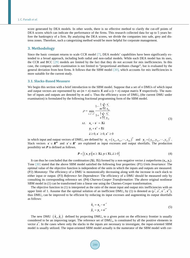
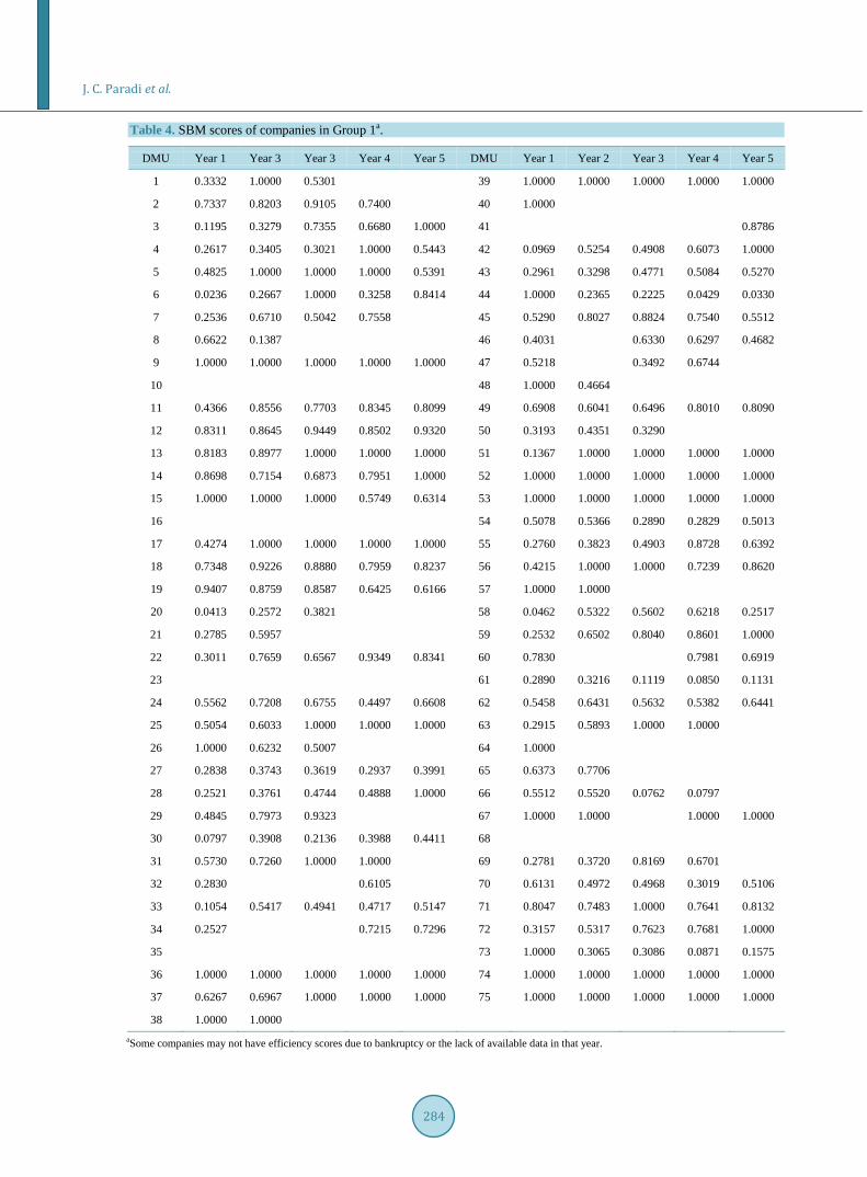
4.2. Results Analysis The companies in Group 1 were evaluated by an input-oriented SBM model for five years, and the results were expressed in Table 4. Once each company was assigned an efficiency score, a measure of bankruptcy status had to be determined. For each year every possible cut-off point was tested at an increment of 0.05 from 0 to 1 to determine the bankrupt and non-bankrupt classification accuracy at those potential cut-off points. Figure 1 shows the accuracy percentages vs. the cross points for the first year. For example for a cut-off point of zero, no bankrupt companies are classified as bankrupt and all non-bankrupt companies would be classified as non- bankrupt. Along with the increasing of cut-off value, the accuracy for non-bankrupt companies is increasing, but the accuracy for bankrupt companies is, on the contrary, are decreasing. The only point which we should choose to maintain highest accuracy for both bankrupt and non-bankrupt companies is the cross point of the two curves.

Table 2. Number of companies in Group 1.

Year before bankruptcy Number of bankrupt companies

Number of non-bankrupt companies

1 40 29

2 34 28

3 31 26

4 32 24

5 26 23

Table 3. Number of companies in Group 2.

Year before bankruptcy Number of bankrupt companies

Number of non-bankrupt companies

1 42 35

2 38 34

3 39 34

4 32 30

5 26 27

Figure 1. Bankrupt & non-bankrupt classification accuracy on year 1.

0.00%10.00%20.00%30.00%40.00%50.00%60.00%70.00%80.00%90.00%

100.00%

0 0.1 0.2 0.3 0.4 0.5 0.6 0.7 0.8 0.9 1

Perc

enta

ge

Cut-off Point

Bankrupt

J. C. Paradi et al.

284

Table 4. SBM scores of companies in Group 1a.

DMU Year 1 Year 3 Year 3 Year 4 Year 5 DMU Year 1 Year 2 Year 3 Year 4 Year 5

1 0.3332 1.0000 0.5301 39 1.0000 1.0000 1.0000 1.0000 1.0000

2 0.7337 0.8203 0.9105 0.7400 40 1.0000

3 0.1195 0.3279 0.7355 0.6680 1.0000 41 0.8786

4 0.2617 0.3405 0.3021 1.0000 0.5443 42 0.0969 0.5254 0.4908 0.6073 1.0000

5 0.4825 1.0000 1.0000 1.0000 0.5391 43 0.2961 0.3298 0.4771 0.5084 0.5270

6 0.0236 0.2667 1.0000 0.3258 0.8414 44 1.0000 0.2365 0.2225 0.0429 0.0330

7 0.2536 0.6710 0.5042 0.7558 45 0.5290 0.8027 0.8824 0.7540 0.5512

8 0.6622 0.1387 46 0.4031 0.6330 0.6297 0.4682

9 1.0000 1.0000 1.0000 1.0000 1.0000 47 0.5218 0.3492 0.6744

10 48 1.0000 0.4664

11 0.4366 0.8556 0.7703 0.8345 0.8099 49 0.6908 0.6041 0.6496 0.8010 0.8090

12 0.8311 0.8645 0.9449 0.8502 0.9320 50 0.3193 0.4351 0.3290

13 0.8183 0.8977 1.0000 1.0000 1.0000 51 0.1367 1.0000 1.0000 1.0000 1.0000

14 0.8698 0.7154 0.6873 0.7951 1.0000 52 1.0000 1.0000 1.0000 1.0000 1.0000

15 1.0000 1.0000 1.0000 0.5749 0.6314 53 1.0000 1.0000 1.0000 1.0000 1.0000

16 54 0.5078 0.5366 0.2890 0.2829 0.5013

17 0.4274 1.0000 1.0000 1.0000 1.0000 55 0.2760 0.3823 0.4903 0.8728 0.6392

18 0.7348 0.9226 0.8880 0.7959 0.8237 56 0.4215 1.0000 1.0000 0.7239 0.8620

19 0.9407 0.8759 0.8587 0.6425 0.6166 57 1.0000 1.0000

20 0.0413 0.2572 0.3821 58 0.0462 0.5322 0.5602 0.6218 0.2517

21 0.2785 0.5957 59 0.2532 0.6502 0.8040 0.8601 1.0000

22 0.3011 0.7659 0.6567 0.9349 0.8341 60 0.7830 0.7981 0.6919

23 61 0.2890 0.3216 0.1119 0.0850 0.1131

24 0.5562 0.7208 0.6755 0.4497 0.6608 62 0.5458 0.6431 0.5632 0.5382 0.6441

25 0.5054 0.6033 1.0000 1.0000 1.0000 63 0.2915 0.5893 1.0000 1.0000

26 1.0000 0.6232 0.5007 64 1.0000

27 0.2838 0.3743 0.3619 0.2937 0.3991 65 0.6373 0.7706

28 0.2521 0.3761 0.4744 0.4888 1.0000 66 0.5512 0.5520 0.0762 0.0797

29 0.4845 0.7973 0.9323 67 1.0000 1.0000 1.0000 1.0000

30 0.0797 0.3908 0.2136 0.3988 0.4411 68

31 0.5730 0.7260 1.0000 1.0000 69 0.2781 0.3720 0.8169 0.6701

32 0.2830 0.6105 70 0.6131 0.4972 0.4968 0.3019 0.5106

33 0.1054 0.5417 0.4941 0.4717 0.5147 71 0.8047 0.7483 1.0000 0.7641 0.8132

34 0.2527 0.7215 0.7296 72 0.3157 0.5317 0.7623 0.7681 1.0000

35 73 1.0000 0.3065 0.3086 0.0871 0.1575

36 1.0000 1.0000 1.0000 1.0000 1.0000 74 1.0000 1.0000 1.0000 1.0000 1.0000

37 0.6267 0.6967 1.0000 1.0000 1.0000 75 1.0000 1.0000 1.0000 1.0000 1.0000

38 1.0000 1.0000 aSome companies may not have efficiency scores due to bankruptcy or the lack of available data in that year.

J. C. Paradi et al.

285

Here that point would be 0.55, where the bankrupt and non-bankrupt accuracies are 67.50% and 68.97% sepa-rately.

To categorize all the companies into three zones, i.e. safe, grey and distress, we need to choose two cut-off points. If we plot the curve of total accuracy which correctly categorized both bankrupt and non-bankrupt com-panies in Figure 2, we can find two points gaining relatively higher total accuracy around the point 0.55. One point is 0.5 located at left with 63.77% overall accuracy. Here the bankrupt companies have a classification ac-curacy of 57.50% and the non-bankrupt companies have a classification accuracy of 72.41%. This point is thus considered to be the bottom cut-off point to discriminate between “distress” and “grey” zones. In the same way, we could fix the top cut-off point 0.6, where the total accuracy obtains another high value. At this point, the classification accuracy for bankrupt companies is 75.00%, and for non-bankrupt companies the classification accuracy is 68.97%. It follows that this point is regarded as the boundary to separate “grey” and “safe” zones.

However, this is only the process to select cut-off points for one year before bankruptcy. In the same way, we can plot the bankrupt and non-bankrupt percentage curves for the other four years before bankruptcy as shown in Figure 3. As we are more concerned about the classification accuracy for bankrupt companies than non- bankrupt, we will shift these points up. By comparing the values over the 5 years, the finalized cut-off points are indicated in Table 5.

Then we calculate the SBM efficiency scores for all companies in Group 2 as shown in Table 6. Based on the cut-off points that we obtained from Group 1, the classification accuracy of Group 2 is estimated as shown in

Figure 2. Selection of bottom & top cut-off points for year 1.

Figure 3. Cut-off points from year 2 to 5 before bankruptcy.

Table 5. Cut-off points for SBM model.

Interval Classification

θ ≥ 0.80 Safe area

0.65 < θ < 0.80 Grey area

θ ≤ 0.65 Distress area

0.00%10.00%20.00%30.00%40.00%50.00%60.00%70.00%80.00%90.00%

100.00%

0 0.1 0.2 0.3 0.4 0.5 0.6 0.7 0.8 0.9 1

Perc

enta

ge

Cut-off Point

Bankrupt

Non-bankrupt

Total Accuracy

J. C. Paradi et al.

286

Table 6. SBM scores of companies in Group 2.

DMU Year 1 Year 2 Year 3 Year 4 Year 5 DMU Year 1 Year 2 Year 3 Year 4 Year 5

1 0.4671 0.4759 0.8892 0.6681 45 0.4436 0.3974 0.3599 0.3616 0.3761

2 1.0000 1.0000 1.0000 0.2977 0.2322 46 1.0000 0.5314 0.3608 1.0000

3 0.1937 0.1681 0.4395 1.0000 1.0000 47 0.0804 0.4013 0.5014 0.3332 0.5777

4 1.0000 1.0000 1.0000 1.0000 1.0000 48 0.8082 0.8554 1.0000 1.0000 1.0000

5 1.0000 1.0000 1.0000 49 1.0000

6 0.8034 0.7558 0.7553 0.7346 0.7413 50 0.1158 1.0000 1.0000

7 1.0000 51 0.6579 0.6973 1.0000 1.0000

8 0.3124 0.1162 0.2337 0.0780 0.3352 52 1.0000 1.0000 1.0000 1.0000

9 0.7817 1.0000 1.0000 1.0000 1.0000 53 0.1583 0.1210

10 1.0000 1.0000 1.0000 1.0000 1.0000 54

11 1.0000 0.7980 0.8862 0.7704 1.0000 55 0.5178 0.8522 1.0000 0.6867 0.8104

12 0.8331 0.8436 0.8684 0.7623 0.8106 56 1.0000 1.0000 1.0000 1.0000 1.0000

13 1.0000 57 0.2558 0.2681 0.2842 0.3289 0.3169

14 0.7181 0.7218 0.7402 0.7745 0.7522 58

15 1.0000 1.0000 1.0000 1.0000 1.0000 59 0.3390 1.0000 1.0000 1.0000 1.0000

16 1.0000 1.0000 60 1.0000 1.0000 1.0000 1.0000 1.0000

17 0.5071 61 0.6462 0.6888 0.7641

18 1.0000 1.0000 1.0000 1.0000 1.0000 62 0.4321 0.4194 0.2214 0.0854

19 0.7484 0.7180 1.0000 1.0000 1.0000 63 0.6317 0.5374 0.3726 0.4164 0.8570

20 1.0000 1.0000 1.0000 64 0.4923 1.0000 0.5715 1.0000

21 0.7149 0.7908 0.8061 0.8125 0.7356 65 0.2869 0.0583

22 0.5457 0.7382 0.7422 0.7398 0.7827 66 0.3773 1.0000 1.0000

23 0.5489 0.5966 0.7836 0.7915 0.8103 67

24 0.9612 1.0000 1.0000 1.0000 68 0.4057 1.0000 1.0000 1.0000 0.3515

25 0.4143 0.8312 0.7234 69 0.5086 0.2944 0.2849 0.5566

26 0.7259 0.6940 0.8135 0.9357 70 1.0000 1.0000 1.0000 1.0000 1.0000

27 0.2709 0.3241 1.0000 0.3093 71 1.0000 1.0000 1.0000 1.0000 1.0000

28 1.0000 1.0000 1.0000 0.7705 72 0.7755 0.7534 0.8137

29 1.0000 1.0000 1.0000 1.0000 1.0000 73 0.6239 0.8440 0.7942 0.7603 0.8238

30 0.2523 0.4529 0.6730 0.7045 0.7190 74 1.0000 1.0000 0.9698 1.0000 0.7284

31 1.0000 1.0000 0.2037 0.2280 0.2174 75

32 0.9831 1.0000 1.0000 76 0.0678 0.2259

33 0.0642 0.2547 0.4764 0.2980 0.4990 77 1.0000 1.0000

34 0.0849 0.7486 1.0000 78 0.3308 0.7783 0.7480

35 0.7423 0.8097 0.8222 0.8360 0.8322 79 0.1245 0.1287 0.1528 0.0210 0.2408

36 0.6434 0.6370 0.5614 80 0.0178 0.0174 0.2678 0.7109 0.7527

37 1.0000 1.0000 1.0000 1.0000 81 0.0365 0.6094 0.5679 0.5794 0.4947

38 0.3789 0.5783 0.6040 0.6271 0.8892 82 0.2689 0.4840 0.4683 0.5283 0.5244

39 0.7512 0.7386 0.7556 0.7820 0.9853 83 0.0090 0.3145 0.6571 0.5638

40 0.2567 0.6749 0.6628 0.7110 84 0.5370 0.7060 0.4407 0.6724 0.2925

41 1.0000 1.0000 1.0000 1.0000 1.0000 85

42 0.3825 0.6303 1.0000 86 0.9606 0.7091 1.0000 1.0000

43 0.4176 0.5269 0.3268 0.2887 0.2596 87 0.2930 0.6173 0.5420

44 0.2386 0.0130 0.0453 0.0398

J. C. Paradi et al.

287

Table 7. Moreover, the classification accuracy results for Group 2 can also be obtained by Altman’s Z'' model, which are shown in Table 8. By comparing the calculation results of Table 7 and Table 8, we find out that some fields of the classification accuracies by SBM may be lower than Altman’s model. However, most of the fields obtained by SBM gain better performance than Altman’s model. If we investigate the overall classifica-tion accuracy including both bankrupt and non-bankrupt companies, and plot the results in Figure 4. It is ap-parently that SBM is entirely better than Altman’s model. Moreover, the longer before bankruptcy happened, the higher accuracy SBM could provide.

5. Conclusions This research surveyed the related literature in bankruptcy prediction, stretching from Beaver’s univariate model to Altman’s Z'' model, then proposed the approach of utilizing a nonparametric method, i.e. the SBM model in DEA, to predict corporate failure. To deal with negative factors in this study, we split such factors into positive and negative parts, which could be a viable option when needed in DEA analyses. Based on the methodological revision to SBM, we also validate our method by two groups of bankrupt and non-bankrupt firms. The second group is examined with the cut-off points obtained from the first group.

The overall accuracy of the SBM model was obviously higher than that of the Altman Z'' model, which showed that the total assets or liabilities of a company were actually not necessary in predicting bankruptcy, and that SBM could be a more appropriate method in corporate failure prediction. The results are significant for companies like non-manufacturing or retail companies which do not own a large investment in assets, and not suitable for using Altman’s Z'' model. The overall classification results showed that Altman Z'' model had good prediction accuracy in the close years before bankruptcy, but still lower than the SBM model developed here, Table 7. Classification accuracy of Group 2 by determined cut-off points.

Year 1 2 3 4 5

Bankrupt accuracy 78.6% 57.9% 46.2% 53.1% 38.5%

Non-bankrupt accuracy 62.9% 61.8% 73.5% 66.7% 70.4%

Total accuracy 71.4% 59.7% 58.9% 59.7% 54.7%

Bankrupt accuracy including grey area 85.7% 68.4% 69.2% 78.1% 57.7%

Non-bankrupt accuracy including grey area 77.1% 88.2% 88.2% 93.3% 81.5%

Total accuracy including grey area 81.8% 77.8% 78.1% 85.5% 69.8%

Total bankruptcy 53.3% 36.1% 30.1% 30.7% 28.3%

Total non-bankrupt 36.4% 45.8% 50.7% 43.6% 56.6%

Total within grey area 10.4% 18.1% 19.2% 25.8% 15.1%

Table 8. Results of Altman Z'' model on Group 2.

Year 1 2 3 4 5

Bankrupt accuracy 77.8% 59.1% 50.0% 41.5% 35.1%

Non-bankrupt accuracy 47.5% 52.5% 55.0% 52.5% 63.9%

Total accuracy 63.5% 55.9% 52.4% 46.9% 49.3%

Bankrupt accuracy including grey area 88.9% 86.4% 70.5% 70.7% 83.8%

Non-bankrupt accuracy including grey area 60.0% 72.5% 75.0% 75.0% 88.9%

Total accuracy including grey area 72.9% 69.1% 59.5% 60.5% 67.1%

Total bankruptcy 61.2% 45.2% 39.3% 34.6% 30.1%

Total non-bankrupt 29.4% 34.5% 44.1% 46.9% 52.1%

Total within grey area 11.8% 23.8% 20.2% 25.9% 36.9%

J. C. Paradi et al.

288

Figure 4. Total classification accuracy comparison between Altman & SBM.

which, in fact, shows a dramatically higher accuracy than Altman’s Z'' model, unveiling a company’s health status in advance, which should be more important for company management (they could change the course of the firm before too late) or investors or lenders (where they could force a change in management, or simply withdraw their investment while there is time).

This research has many useful conclusions but, as usual, there are suggestions for further work, including: 1) employing alternate DEA models or constraint conditions, particularly using the Assurance Region model which will put more restrictions on the variable weights and may obtain more meaningful results; 2) prediction accu-racy may be affected by different approaches to selecting inputs/outputs, therefore different or other, related fi-nancial factors may bring higher prediction accuracy; 3) due to the lack of available data, the number of DMUs used in this study was insufficient for a more comprehensive assessment of the model. With a larger number of DMUs, the cut-off points will become more realistic and accurate for bankruptcy prediction; 4) innovative ap-proaches to determine the cut-off points could be explored. The trial and error approach is simple and intuitive, however a different and more statistically sound method could be developed. Decision trees were considered but not employed, and this could be considered for future research.

Either previous univariate models or Altman’s Z and Z'' models mostly focused on firm asset size, and used parametric methods, i.e. weighted sum of asset based items, which resulted in more likely an empirical cut-off points selecting process, but not a data based reality. It follows that the DEA technique, a non-parametric method, could solve the problem resulting in a rather practical approach to predict corporate failure, especially for non-manufacturing firms. In closing, we hope that this research will be insightful and informative for future researchers.

References [1] Beaver, W.H. (1967) Financial Ratios as Predictor of Failure. Journal of Accounting Research, 5, 71-111. [2] Altman, E. (1968) Financial Ratios, Discriminant Analysis and the Prediction of Corporate Bankruptcy. Journal of Fi-

nance, 23, 589-609. http://dx.doi.org/10.1111/j.1540-6261.1968.tb00843.x [3] Grice, J. and Ingram, R. (2001) Tests of the Generalizability of Altman’s Bankruptcy Prediction Model. Journal of

Business Research, 54, 53-61. http://dx.doi.org/10.1016/S0148-2963(00)00126-0 [4] Stephen, H., Keating, E., et al. (2004) Assessing the Probability of Bankruptcy. Review of Accounting Studies, 9, 5-34.

http://dx.doi.org/10.1023/B:RAST.0000013627.90884.b7 [5] The World Bank (2011) Growth of the Service Sector.

http://www.worldbank.org/depweb/beyond/beyondco/beg_09.pdf [6] Altman, E. (2002) Bankruptcy, Credit Risk and High Yield Junk Bonds. Blackwell Publishers Inc., Malden. [7] Charnes, A., Cooper, W.W. and Rhodes, E. (1978) Measuring the Efficiency of Decision Making Units. European

Journal of Operational Research, 2, 429-444. http://dx.doi.org/10.1016/0377-2217(78)90138-8 [8] Farrell, M.J. (1957) The Measurement of Productive Efficiency. Journal of the Royal Statistical Society Series A, 120,

253-290. http://dx.doi.org/10.2307/2343100 [9] Emrouznejad, A., Parker, B.R. and Tavares, G. (2008) Evaluation of Research in Efficiency and Productivity: A Sur-

J. C. Paradi et al.

289

vey and Analysis of the First 30 Years of Scholarly Literature in DEA. Socio-Economic Planning Sciences, 42, 151- 157. http://dx.doi.org/10.1016/j.seps.2007.07.002

[10] Paradi, J.C. and Zhu, H. (2013) A Survey on Bank Branch Efficiency and Performance Research with Data Envelop-ment Analysis. Omega, 41, 61-79. http://dx.doi.org/10.1016/j.omega.2011.08.010

[11] Liu, J.S., Lu, L.Y., Lu, W.M. and Lin, B.J. (2013) Data Envelopment Analysis 1978-2010: A Citation-Based Literature Survey. Omega, 41, 3-15. http://dx.doi.org/10.1016/j.omega.2010.12.006

[12] Yang, X. and Morita, H. (2013) Efficiency Improvement from Multiple Perspectives: An Application to Japanese Banking Industry. Omega, 41, 501-509. http://dx.doi.org/10.1016/j.omega.2012.06.007

[13] Alexander, S.S. (1949) The Effect of Size of Manufacturing Corporation on the Distribution of the Rate of Return. Re-view of Economics and Statistics, 31, 229-235. http://dx.doi.org/10.2307/1927749

[14] Deakin, E. (1972) A Discriminant Analysis of Predictors of Business Failure. Journal of Accounting Research, 10, 167-179. http://dx.doi.org/10.2307/2490225

[15] Ohlson, J.A. (1980) Financial Ratios and the Probabilistic Prediction of Bankruptcy. Journal of Accounting Research, 18, 109-131. http://dx.doi.org/10.2307/2490395

[16] Zmijewski, M.E. (1984) Methodological Issues Related to the Estimation of Financial Distress Prediction Models. Journal of Accounting Research, 22, 59-82. http://dx.doi.org/10.2307/2490859

[17] Hsieh, S.J. (1993) A Note on the Optimal Cutoff Point in Bankruptcy Prediction Models. Journal of Business Finance and Accounting, 30, 457-464. http://dx.doi.org/10.1111/j.1468-5957.1993.tb00268.x

[18] Grice, J.S. and Dugan, M. (2001) The Limitations of Bankruptcy Prediction Models: Some Cautions for the Researcher. Review of Quantitative Finance and Accounting, 17, 151-166. http://dx.doi.org/10.1023/A:1017973604789

[19] Shumway, T. (2001) Forecasting Bankruptcy More Accurately: A Simple Hazard Model. Journal of Business, 74, 101- 124. http://dx.doi.org/10.1086/209665

[20] Grice, J.S. and Ingram, R.W. (2001) Tests of the Generalizability of Altman’s Bankruptcy Prediction Model. Journal of Business Research, 54, 53-61. http://dx.doi.org/10.1016/S0148-2963(00)00126-0

[21] Chava, S. and Jarrow, R. (2004) Bankruptcy Prediction with Industry Effects. Review of Finance, 8, 537-569. http://dx.doi.org/10.1093/rof/8.4.537

[22] Premachandra, I., Chen, Y. and Watson, J. (2011) DEA as a Tool for Predicting Corporate Failure and Success: A Case of Bankruptcy Assessment. Omega, 39, 620-626. http://dx.doi.org/10.1016/j.omega.2011.01.002

[23] Li, Z., Crook, J. and Andreeva, G. (2014) Chinese Companies Distress Prediction: An Application of Data Envelop-ment Analysis. Journal of the Operational Research Society, 65, 466-479. http://dx.doi.org/10.1057/jors.2013.67

[24] Shetty, U., Pakkala, T. and Mallikarjunappa, T. (2012) A Modified Directional Distance Formulation of DEA to As-sess Bankruptcy: An Application to IT/ITES Companies in India. Expert Systems with Applications, 39, 1988-1997. http://dx.doi.org/10.1016/j.eswa.2011.08.043

[25] Xu, X. and Wang, Y. (2009) Financial Failure Prediction Using Efficiency as a Predictor. Expert Systems with Appli-cations, 36, 366-373. http://dx.doi.org/10.1016/j.eswa.2007.09.040

[26] Cielen, A., Peeters, L. and Vanhoof, K. (2004) Bankruptcy Prediction Using a Data Envelopment Analysis. European Journal of Operational Research, 154, 526-532. http://dx.doi.org/10.1016/S0377-2217(03)00186-3

[27] Sueyoshi, T. and Goto, M. (2009) Methodological Comparison between DEA (Data Envelopment Analysis) and DEA-DA (Discriminant Analysis) from the Perspective of Bankruptcy Assessment. European Journal of Operational Research, 199, 561-575. http://dx.doi.org/10.1016/j.ejor.2008.11.030

[28] Yeh, C.C., Chi, D.J. and Hsu, M.F. (2010) A Hybrid Approach of DEA, Rough Set and Support Vector Machines for Business Failure Prediction. Expert Systems with Applications, 37, 1535-1541. http://dx.doi.org/10.1016/j.eswa.2009.06.088

[29] Banker, R.D., Charnes, A. and Cooper, W. (1984) Some Models for Estimating Technical and Scale Inefficiencies in Data Envelopment Analysis. Management Science, 30, 1078-1092. http://dx.doi.org/10.1287/mnsc.30.9.1078

[30] Tone, K. (2001) A Slacks-Based Measure of Efficiency in Data Envelopment Analysis. European Journal of Opera-tional Research, 130, 498-509. http://dx.doi.org/10.1016/S0377-2217(99)00407-5

[31] Cooper, W.W., Seiford, L.M. and Tone, K. (2007) Data Envelopment Analysis: A Comprehensive Text with Models, Applications, References and DEA-Solver Software. 2nd Edition, Springer, Berlin, 333-335.

[32] Staat, M. (2001) The Effect of Sample Size on the Mean Efficiency in DEA: Comment. Journal of Productivity Analy-sis, 15, 129-137. http://dx.doi.org/10.1023/A:1007826405826

[33] Zhang, Y. and Bartels, R. (1998) The Effect of Sample Size on the Mean Efficiency in DEA with an Application to Electricity Distribution in Australia, Sweden and New Zealand. Journal of Productivity Analysis, 9, 187-204.

J. C. Paradi et al.

290

http://dx.doi.org/10.1023/A:1018395303580 [34] Smith, P. (1997) Model Misspecification in Data Envelopment Analysis. Annals of Operations Research, 73, 233-252.

http://dx.doi.org/10.1023/A:1018981212364 [35] Banker, R.D., Chang, H. and Cooper, W.W. (1996) Simulation Studies of Efficiency, Returns to Scale and Misspecifi-

cation with Nonlinear Functions in DEA. Annals of Operations Research, 66, 233-253. http://dx.doi.org/10.1007/BF02187300

[36] Panagiotis, Z. (2012) Dealing with Small Samples and Dimensionality Issues in Data Envelopment Analysis. http://mpra.ub.uni-muenchen.de/39226/

[37] Sergio, P. and Daniel, S. (2009) How to Generate Regularly Behaved Production Data? A Monte Carlo Experimenta-tion on DEA Scale Efficiency Measurement. European Journal of Operational Research, 199, 303-310. http://dx.doi.org/10.1016/j.ejor.2008.11.013

[38] Mergent, I. (2011) Mergent Online. http://www.mergentonline.com/ [39] Charles, L.M. (1942) Financing Small Corporations in Five Manufacturing Industries, 1926-36. National Bureau of

Economic Research, Cambridge.