Data-Driven Robust Optimization Based on Kernel Learning

Chao Shanga, Xiaolin Huangb, Fengqi You∗,a

aSmith School of Chemical and Biomolecular Engineering, Cornell University, Ithaca, New York14853, USA

bInstitute of Image Processing and Pattern Recognition, Shanghai Jiao Tong University, Shanghai200400, China

Abstract

We propose piecewise linear kernel-based support vector clustering (SVC) as a new ap-proach tailored to data-driven robust optimization. By solving a quadratic program,the distributional geometry of massive uncertain data can be effectively captured as acompact convex uncertainty set, which considerably reduces conservatism of robust opti-mization problems. The induced robust counterpart problem retains the same type as thedeterministic problem, which provides significant computational benefits. In addition, byexploiting statistical properties of SVC, the fraction of data coverage of the data-drivenuncertainty set can be easily selected by adjusting only one parameter, which furnishesan interpretable and pragmatic way to control conservatism and exclude outliers. Nu-merical studies and an industrial application of process network planning demonstratethat, the proposed data-driven approach can effectively utilize useful information withmassive data, and better hedge against uncertainties and yield less conservative solutions.

Key words: Robust optimization, Uncertainty set, Data-driven methods, Supportvector clustering, Piecewise linear modeling

1. Introduction

In science and engineering, optimization problems are inevitably encountered whenev-er one seeks to make decisions by maximizing/minimizing some certain criterion. Howev-er, real-world parameters are subject to randomness in various degrees, rendering deter-ministic optimization models unreliable in an uncertain environment (Sahinidis [2004]).It has been demonstrated that even a slight perturbation on parameters in an opti-mization problem could exert overwhelming effects on the computed optimal solutions,which results in suboptimality or even infeasibility of optimization problems (Mulveyet al. [1995]). Motivated by the urgent requirement of handling uncertainties in de-cision making, stochastic optimization and robust optimization have received immenseresearch attentions in recent decades (Kall et al. [1994]; Ben-Tal et al. [2009]; Birge and

∗To whom all correspondence should be addressed: Tel: +1 (607)255-1162; Fax: +1 (607)255-9166;E-mail: fengqi.you@cornell.edu

Email addresses: chao.shang@cornell.edu (Chao Shang), xiaolinhuang@sjtu.edu.cn (XiaolinHuang), fengqi.you@cornell.edu (Fengqi You)

Preprint submitted to Computers & Chemical Engineering June 2, 2017

Louveaux [2011]; Bertsimas et al. [2011]; Gabrel et al. [2014]; Yuan et al. [2015]), whichhedge against uncertainties by bringing in conservatism. Stochastic optimization entailscomplete knowledge about the underlying probability distribution of uncertainties, whichmay be unrealistic in practice. As an effective alternative, robust optimization takes adeterministic and set-based way to model uncertainties, and balance between the mod-eling power and computational tractability, which has obtained considerable attentionsrecently in the realm of process systems engineering. Typical applications include pro-cess network design (Gong et al. [2016]; Gong and You [2017]), supply chain management(Tong et al. [2014]; Yue and You [2016]), and process scheduling (Lappas and Gounaris[2016]; Shi and You [2016]).

A paramount ingredient in robust optimization is to construct an uncertainty setincluding probable realizations of uncertain parameters. The earliest attempts in for-mulating uncertainty sets date back to the 1970s, with the work of Soyster [1973], inwhich coefficients are perturbed by uncertainties distributed in a known box. Despiteits computational convenience and guaranteed feasibility, the box uncertainty set tendsto induce over-conservative decisions. Later, immense research effort has been made ondevising more flexible robust models to ameliorate over-conservatism. Ellipsoidal uncer-tainty sets have been put forward independently by El Ghaoui et al. [1998]; Ben-Tal andNemirovski [1998, 1999], based on which the robust counterpart model simplifies to aconic quadratic problem in the presence of linear constraints. To enhance the model-ing flexibilities, intersections of basic uncertainty sets have been designed, including the“interval+ellipsoidal” uncertainty set (Ben-Tal and Nemirovski [2000]) and the “inter-val+polyhedral” uncertainty set. Bertsimas and Sim [2004] robustify linear programsusing a polyhedral uncertainty set adjustable with the so-called budget, which turns outto be identical to the “interval+polyhedral” uncertainty set. Interested readers are re-ferred to review papers (Bertsimas et al. [2011]; Gabrel et al. [2014]) and the monograph(Ben-Tal et al. [2009]) for a comprehensive overview of uncertainty sets-induced robustoptimization methods.

Despite the burgeoning prevalence of uncertainty set-induced robust optimization, apotential limitation is that uncertainties in each dimension are assumed as being inde-pendently and symmetrically distributed. The issue of data correlation is first addressedby Bertsimas and Sim [2004], in which correlated uncertainties are disentangled by meansof an underlying source of independent uncertainties, expressed as:

aij = aij +∑k∈Ki

ηikgkj . (1)

where aij stands for the nominal value, and ηik denotes the source of indepen-dent uncertainties. Ferreira et al. [2012] suggest determining the values of aij andgkj by means of principal component analysis (PCA) and minimum power decomposi-tion (MPD). Based on (1), classical symmetric uncertainty sets are generalized by Yuanet al. [2016], and explicit formulations of their robust counterparts are also provided.Jalilvand-Nejad et al. [2016] devise correlated polyhedral uncertainty sets using second-order statistical information from historical data. In regard to asymmetric uncertainties,Chen et al. [2007] adopt the forward and backward deviations to capture distributionalasymmetry through the norm-induced uncertainty set while still preserving its tractabil-ity. In Natarajan et al. [2008], a modified Value-at-Risk (VaR) measure is developed andinvestigated by taking into account asymmetries in the distributions of portfolio returns.

2

A prominent and practical issue of uncertainty set-induced robust optimization ishow to determine the set coefficients appropriately, which are in general assumed asknown according to domain-specific knowledge. In the absence of first-principle knowl-edge, leveraging available historical data provides a practical way to characterize thedistributional information. For instance, the lower and the upper bounds of an intervalcan be specified as the minimum and the maximum of observed data samples, albeitconservatively. More sophisticated approaches make use of variance and covariance ofhistorical data, which renders the model statistically interpretable (Pachamanova [2002];Bertsimas and Pachamanova [2008]; Ferreira et al. [2012]). An alternative streamline ofdata-driven optimization is the distributionally robust optimization, which utilizes bothdata and hypothesis tests to construct the ambiguity set including P at a high confidencelevel (Delage and Ye [2010]; Jiang and Guan [2016]; Bertsimas et al. [2017]). However,one still needs to specify the the type of hypothesis tests to yield a reliable solution,and the induced optimization problem is generally difficult to solve (Hanasusanto et al.[2017]). For example, the moment-based hypothesis test typically leads to reformula-tions in terms of linear matrix inequalities and bilinear matrix inequalities (Delage andYe [2010]; Zymler et al. [2013]), which erect obstacles to further tackle mixed-integerand large-scale problems that are commonly encountered in process systems engineering.In this work, we hence focus on uncertainty set-based robust optimization with betterapplicability and implementation convenience.

In real-world applications, the underlying distribution P of uncertainties may be in-trinsically complicated and vary under different circumstances. When one is faced withhigh-dimensional uncertainties, it is rather challenging to choose the type of uncertaintysets by prior knowledge, tune the coefficients, and further evaluate its divergence withthe true underlying distribution P. In the era of big data, a significant amount of datacollected routinely themselves embody abundant information about P, thereby pavingnew way for further advancing decision making tools (Bertsimas et al. [2011]; Qin [2014]).A desirable uncertainty set shall flexibly adapt to the intrinsic structure behind data,thereby well characterizing P and ameliorating the suboptimality of solutions. Froma machine learning perspective, constructions of uncertainty sets based upon historicaldata can be viewed as an unsupervised learning problem. There have been a plethoraof effective unsupervised learning models, for example, kernel density estimation (KDE)and support vector machines (SVM), which could provide powerful representations of da-ta distributions (Bishop [2006]). In principle, one could resort to such machine learningtools to estimate data densities with sufficient accuracies; nevertheless, it remains a chal-lenging task to formulate an appropriate uncertainty set for modeling robust optimizationproblems. This is mainly because complicating nonlinear items, such as the radial basisfunction (RBF) exp−x2/2σ2 and the sigmoid function tanh(γx + r), dominate con-ventional machine learning models, which invariably prohibit an analytical treatment ofrobust optimization problems, especially a tractable robust counterpart reformulation.This may somewhat explain the scarce of applications of machine learning models inrobust optimization all this time.

In this paper, we propose an effective data-driven approach for robust optimizationthat is tailored to uncertainty set constructions as well as computational implementation-s, thereby bridging machine learning and robust optimization directly. As an extendedSVM technology, support vector clustering (SVC) has been extensively adopted to es-timate the support of an unknown probability distribution from random data samples

3

(Scholkopf et al. [1999],Muller et al. [2001]). A particular merit of SVC is that it hastheoretical underpinnings in statistical learning theory (Vapnik [2013]), and enjoys de-sirable generalization performance in face of real-world problems (Lee and Lee [2005]).Instead of using the ubiquitous RBF kernel involving intricate nonlinearities, a novelpiecewise linear kernel, referred to as the generalized intersection kernel, is proposed inthis work to formulate the SVC model, which entails solving a quadratic program (QP)only. Thanks to the kernel formulation, the SVC model could not only handle correlat-ed uncertainties and lead to asymmetric uncertainty sets, but also enjoys an adaptivecomplexity, thereby featuring a nonparametric scheme. Most importantly, it leads to aconvex polyhedral uncertainty set, thereby rendering the robust counterpart problem ofthe same type as the deterministic problem, which provides computational convenience.If the deterministic problem is an MILP, then the robust counterpart problem can bealso cast as an MILP. In this way, a satisfactory trade-off can be achieved between mod-eling power of SVC and computational convenience of robust optimization. Moreover, weshow that the parameters to be tuned bear explicit statistical implications, which allowone to easily control the conservatism as well as the complexity of the induced robustoptimization problems. Numerical and application case studies are conducted to showthe practicability and efficacy of the proposed data-driven approach in hedging againstuncertainties and alleviating the conservatism of robust solutions.

The layout of this paper is organized as follows. Section 2 revisits the convention-al uncertainty sets for robust optimization, and the SVC-based unsupervised learningschema. In Section 3, the piecewise linear kernel-based SVC is proposed, along with theinduced data-driven uncertainty set. Its properties are also discussed from various as-pects, including the parameter interpretation, asymptotic behavior, and computationaltractability. Section 4 is devoted to a comprehensive numerical evaluation on the perfor-mance of the proposed approach compared with classical ones. In Section 5, case studieson an application of process network planning are performed, followed by concludingremarks in Section 6.

2. Preliminaries

2.1. Uncertainty set induced robust optimization

We consider the following simple linear optimization problem:

minx∈X

cTx

s.t. Ax ≤ b(2)

where x ∈ Rn stands for the decision variables. Without loss of generality, we couldassume that only the left-hand side (LHS) coefficients are contaminated by uncertainties.Specifically, we target on a single linear constraint, and suppress its dependence on theconstraint index for notational brevity:∑

k

akxk ≤ b. (3)

In most robust optimization literature, the uncertainty is often decomposed as (El Ghaouiet al. [1998]; Ben-Tal and Nemirovski [1999]; Pachamanova [2002]; Bertsimas and Sim

4

[2004]):ak = ak + ukak, ∀k (4)

where ak represents the “nominal” value of ak, ak denotes the “magnitude” of the randomperturbation, and uk is a “normalized” random variable whose support is centered atthe origin. Given an uncertainty set U that u = [u1, u2, · · · , un]T belongs to, one alwaysseeks to ensure the constraint satisfaction under all possible scenarios within U , expressedas: ∑

k

akxk + maxu∈U

∑k

ukakxk ≤ b. (5)

As with the selection of the uncertainty set U , we mention five basic uncertainty setsherein:

• Box uncertainty setU∞ = u||uk| ≤ Ψ, ∀k (6)

• Polyhedral uncertainty set

U1 =

u

∣∣∣∣∣∑k

|uk| ≤ Γ

(7)

• Ellipsoidal uncertainty set

U2 =

u

∣∣∣∣∣∑k

u2k ≤ Ω2

(8)

• Interval + Polyhedral uncertainty set (Gamma uncertainty set)

U1∩∞ =

u

∣∣∣∣∣∑k

|uk| ≤ Γ, |uk| ≤ 1, ∀k

(9)

• Interval + Ellipsoidal uncertainty set

U2∩∞ =

u

∣∣∣∣∣∑k

u2k ≤ Ω2, |uk| ≤ 1, ∀k

(10)

Note that the uncertainty spreads symmetrically and radially from the origin in the aboveuncertainty sets (6)-(10), and their sizes are controlled by budget parameters Ψ,Ω,Γ.Based on norms, they result in succinct formulations of the robust counterpart problemby means of dual norms, which provide computational convenience.

In practical applications, however, classical uncertainty sets still show some limita-tions. On one hand, their geometric structures are fixed a priori, and there is no warrantyfor an agreement with the support of the true distribution P. In face of complicated dis-tributional geometry, the modeling power of classical uncertainty sets is quite limited.On the other hand, one should determine the nominal values ak as well as the magni-tudes ak carefully in the absence of first-principle knowledge. It is a nontrivial task to

5

obtain the exact information of these parameters empirically using historical data. Evenif the budget parameters Ψ,Ω,Γ can be specified based on the established probabilisticguarantees (see, e.g., Li and Floudas [2012]; Guzman et al. [2016, 2017]), a poor specifi-cation of ak and ak can still incur suboptimal solutions. Recently, researchers haveproposed to adopt machine learning techniques such as the Dirichlet process mixturemodel to directly learn the uncertainty set U from data D (Ning and You [2017a,b]),such that distributional information can be automatically encompassed in U and over-conservatism can be reduced. In this way, the worst-case robust constraint (5) becomes

maxa∈U(D)

aTx ≤ b, (11)

where U(D) exposes the dependence of U on the data D. In the previous work, howev-er, tedious nonconvex optimization algorithms such the variational Bayesian algorithmare inevitably encountered in the modeling stage, and there lacks an interpretable wayfor decision makers to control both the conservatism and complexity. In contrast, as awell-known unsupervised kernel learning approach, support vector clustering (SVC) hasproven to be a particularly efficient pattern recognition approach for modeling compli-cated high-dimensional uncertainties, with only convex optimization required (Scholkopfet al. [2001]; Ben-Hur et al. [2001]; Muller et al. [2001]). Most importantly, some u-nique properties in statistical learning theory can be desirably exploited to enhance theapplicability of the induced robust optimization problem (11). Next, we proceed withdata-driven constructions of U(D) with SVC.

2.2. Support vector clustering

SVC aims to give a description of a number of data points by means of an enclosingsphere with minimal volume (Scholkopf et al. [2001]; Ben-Hur et al. [2001]; Muller et al.[2001]), thereby enabling an explicit characterization of new data samples that resembletraining data. Assume that a set D of N data samples D = u(i)Ni=1 are available. Forclear distinctions, here we use superscript and subscript to denote the index of a datasample and a certain dimension of a vector, respectively. Using a nonlinear mappingφ(u) : Rn 7→ RK to a high-dimensional features space F , SVC seeks the smallest spherethat encloses all data by formulating the following optimization problem:

mina,R

R2

s.t. ||φ(u(i))− p||2 ≤ R2, i = 1, · · · , N(12)

where the sphere is centered at p and of radius R. This model is considered as havinga hard margin that includes all samples. To accommodate potential outliers and eschewan unnecessarily large radius R, one could further adopt soft margin by adding slackvariables ξi:

mina,R,ξ

R2 +1

Nν

N∑i=1

ξi

s.t. ||φ(u(i))− p||2 ≤ R2 + ξi, i = 1, · · · , Nξi ≥ 0, i = 1, · · · , N

(13)

6

The objective pursues a sphere of minimal radius, while penalizing violations of outliers.The trade-off between these two different goals is achieved by adjusting the regularizationparameter ν > 0. Introducing the Lagrangian multipliers α and β leads to the followingLagrangian function:

L(p, R, ξ,α,β) = R2 +1

Nν

N∑i=1

ξi −N∑i=1

αi(R2 + ξi − ||φ(u(i))− p||2)−

N∑i=1

βiξi (14)

According to the Karush-Kuhn-Tucker (KKT) conditions, one obtains by takingderivatives to zero:

∂L∂R

= 0→N∑i=1

αi = 1 (15)

∂L∂p

= 0→ p =

N∑i=1

αiφ(u(i)) (16)

∂L∂ξi

= 0→ αi + βi =1

Nν(17)

Eq. (16) indicates that the center p is a linear combination of mappings of all datasamples. Plugging (15)-(17) into (14) results in a disciplined QP as the dual problem:

minα

N∑i=1

N∑j=1

αiαjK(u(i),u(j))−N∑i=1

αiK(u(i),u(j))

s.t. 0 ≤ αi ≤ 1/Nν, i = 1, · · · , NN∑i=1

αi = 1

(18)

The kernel trick K(u(i),u(j)) = φ(u(i))Tφ(u(j)) motivated by the Mercer’s theoremallows for simple computation of inner-products in the feature space F , which may evenhave infinite dimensions. For the kernel function K(·, ·) one typically has the followingoptions: K(u,v) = (uTv + 1)d (polynomial kernel of degree d) (Scholkopf and Smola[2002]), K(u,v) = exp−||u− v||2/2σ2 (RBF kernel with bandwidth σ) (Suykens andVandewalle [1999]) and K(u,v) = tanh(γ · uTv + r) (sigmoid kernel) (Vapnik [2013]).In past decades, the power of such kernels has been verified by a tremendous diversityof applications in pattern recognition and machine learning. Rather, using these kernelsstraightforwardly in robust optimization will give rise to computational intractability, asto be clarified in the sequel.

In order to solve the dual problem (18), standard QP routines can be utilized. Forimproved efficiency, sequential minimal optimization (SMO) procedure can be appliedthanks to the simplicity of the constraints (Platt [1999]). Besides, (18) bears a desirablegeometric interpretation. According to the complementary slackness, we will have αi = 0and βi = 1/Nν for the ith data sample in the interior of the sphere ||φ(u(i)) − p||2 <R2. The other cases can be analyzed in a similar fashion, leading to the following

7

correspondence (Ben-Hur et al. [2001]):

||φ(u(i))− p||2 < R2 → αi = 0, βi = 1/Nν (19)

||φ(u(i))− p||2 = R2 → 0 < αi < 1/Nν, 0 < βi < 1/Nν (20)

||φ(u(i))− p||2 > R2 → αi = 1/Nν, βi = 0 (21)

It can be observed that only data samples u(i) with positive αi, referred to as supportvectors, will contribute to the center p. A portion of them reside exactly on the boundaryof the sphere with ||φ(u(i)) − p||2 = R2, named boundary support vectors, whereas therest with ||φ(u(i))− p||2 > R2 are regarded as outliers. We hence define

SV = i |αi > 0, ∀i (22)

andBSV = i |0 < αi < 1/Nν, ∀i (23)

as the index sets of all support vectors and boundary support vectors, respectively. Be-sides, the radius R can be determined as the distance from the center p to any boundarysupport vector xi′ :

R2 = K(u(i′),u(i′))− 2

N∑i=1

αiK(u(i′),u(i)) +

N∑i=1

N∑j=1

αiαjK(u(i),u(j)), i′ ∈ BSV. (24)

Finally, the region in which a data sample is accepted as normal can be described as:

U(D) =

u

∣∣∣∣∣∣K(u,u)− 2

N∑i=1

αiK(u,u(i)) +

N∑i=1

N∑j=1

αiαjK(u(i),u(j)) ≤ R2

. (25)

Indeed, we could recognize U(D) as a data-driven uncertainty set, which is potentiallyuseful in the robust optimization setting. However, the commonly used kernel functions,such as the polynomial kernel, RBF kernel, and sigmoid kernel, inevitably incorporatesome nonlinear terms, which substantially complicate its applications in robust optimiza-tion. Consider the following simple robust optimization problem exemplified by the RBFkernel:

minx∈X

cTx

s.t. maxu

uTx

∣∣∣∣∣∣2N∑i=1

αie||u(i)−u||2/2σ2

≥ R2 − 1−N∑i=1

N∑j=1

αiαj

≤ b(26)

Due to the penetration of complicating RBF terms, it is notoriously difficult to reckonwith the constraint and derive a desirable dual reformulation, which substantially un-derpins the computational tractability of robust optimization (Bertsimas et al. [2011];Gabrel et al. [2014]).

8

3. Data-Driven Uncertainty Set Induced by Generalized Intersection KernelSVC

In this section, we first propose new a piecewise linear kernel for modeling SVC. Thenwe derive explicit formulations of the induced uncertainty sets, based on which the robustcounterpart can be readily obtained. Well-established properties of SVC are exploitedto facilitate practical use in robust optimization.

3.1. A new piecewise linear kernel for SVC

Now we show that piecewise linear kernels will provide possibilities in obtaining atractable and convex expression of U . What we choose is the piecewise linear kerneltermed as the intersection kernel, which is made popular by Maji et al. [2008, 2013] forimage classification with applications to computer vision:

K(u,v) =

n∑k=1

minuk, vk, (27)

where u,v ∈ Rn+. The attractiveness of (27) lies in two aspects. On one hand, the inter-

section kernel ensures the positive-definiteness of the kernel matrix K = K(u(i),u(j)) 0, thereby preserving the convexity of the dual problem (18), and warranting the globaloptimality as well as modeling performance. On the other hand, by resubstituting (27)into (25), it can be observed that the uncertainty set U will become convex since theintersection kernel function is concave in u and all dual variables αi are non-negative.

Despite such appealing observations, we cannot directly apply the intersection kernelto uncertainty sets construction. Because of the non-negativity of data samples, theinduced separating hyperplane tends to be far away from the origin. Assuming that theuncertainty is bounded, we desire the data cluster to be enclosed in all directions. Giventhat uk < uk < uk, where uk and uk are the lower bound and upper bound a priori, wepropose the following generalized intersection kernel (GIK):

K(u,v) =

n∑k=1

minuk − uk, vk − uk+

n∑k=1

minuk − uk, uk − vk

=

n∑k=1

uk − uk − |uk − vk|

,n∑k=1

lk − ||u− v||1

(28)

where kernel parameters depend only on the interval width lk = uk − uk of interval(uk, uk). GIK is also related to the truncated `1-distance (TL1) kernel K(u,v) =max ρ− ||u− v||1, 0 for pattern classifications (Huang et al. [2017]); however, the trun-cation in TL1 kernel compromises the concavity of the kernel function.

Notice in (28) that each dimension uk of u makes identical contribution to the kernelfunction. However, variables have different scales in practice, and may sometimes be

9

correlated. We hence propose to further incorporate covariation information into GIK,giving rise to the following weighted generalized intersection kernel (WGIK):

K(u,v) =

n∑k=1

lk − ||Q(u− v)||1, (29)

where Q is a weighting matrix, which can be constructed using covariance informationfrom data. An unbiased estimation of the covariance matrix Σ can be attained based onN samples u(i):

Σ =1

N − 1

N∑i=1

u(i)(u(i)

)T−

(N∑i=1

u(i)

)(N∑i=1

u(i)

)T . (30)

The weighting matrix can be constructed as Q = Σ−12 , commonly referred to as the

whitening matrix to eliminate cross-correlations, as typically used in independent com-ponent analysis (ICA) (Hyvarinen et al. [2004]). In this way, each dimension of thetransformed data Qu will be isotropic, and appears to exert similar influence on thekernel expression.

As a major contribution of this work, the proposed WGIK (29) is a new kernel func-tion tailored to modeling uncertainty with SVC in robust optimization. To derive theWGIK-based SVC model, one simply needs to solve the QP (18) with K(·, ·) constructedaccording to (29). Different from conventional kernel functions such as the polynomialkernel and RBF kernel, WGIK function is concave and yields a desirable convex accep-tance region of SVC (25), as to be adopted as the uncertainty set for robust optimization.For kernel learning methods, the parameter selection is a crucial issue that heavily affectsthe model performance. For the proposed WGIK, the width parameters lk have to becarefully tuned, with the aim to ensure the positive-definiteness of the induced kernelmatrix K, as well as the convexity of the dual QP (18). Generally speaking, one cannotarbitrarily choose a function as the kernel function, since the high-dimensional featurespace F exists only when the induced kernel matrix K is positive definite (Scholkopf andSmola [2002]). We hence propose to choose lk according to

lk > max1≤i≤N

qTk u(i) − min

1≤i≤NqTk u(i) (31)

as a simple criterion, which suffices to ensure the positive-definiteness of K by the fol-lowing proposition.

Proposition 1. Assume that kernel parameters lk satisfy (31), then the kernel matrixK with entries K(u(i),u(j)) induced by WGIK (29) is positive definite.

Proof. First denote by z = Qu (z(i) = Qu(i)) the transformed variables in shorthand,and define the residual

εk = lk − max1≤i≤N

qTk u(i) + min

1≤i≤NqTk u(i) > 0 (32)

according to (31). Then we could construct valid upper and lower bounds of zk aszk = max1≤i≤N qT

k ui + εk/2 and zk = min1≤i≤N qTk ui− εk/2, which satisfy lk = zk− zk.

10

It is easy to have K = K++K−, where K+ has entries K+(u(i),u(j)) =∑nk=1 minz(i)k −

zk, z(j)k −zk, and K− has entries K−(ui,uj) =

∑nk=1 minzk−z(i)k , zk−z(j)k . Denoting

by v(i)k = z

(i)k − zk ≥ 0, K+ turns out to be a conventional intersection kernel matrix and

is hence positive definite (Odone et al. [2005]). The positive-definiteness of K− can beestablished in a similar fashion. Therefore, K = K+ + K− is positive definite.

Moreover, we point out that, the selection of lk has no impacts on the induced SVCmodel as long as (31) is satisfied. To address this invariance property, we establish thefollowing proposition.

Proposition 2. Solving the QP (18) yields the same solution αi with lk selectedaccording to (31).

Proof. Assume that there are two different specifications lk and l′k satisfying (31),and their induced kernel matrices are denoted by K and K′, respectively. By definingρ =

∑k(lk − l′k), we have K = K′ + ρ11T. Then solving (18) with K becomes:

minα

αT(K′ + ρ11T)α−

(ρ+

∑k

l′k

)·αT1

s.t. 0 ≤ αi ≤ 1/Nν, i = 1, · · · , NαT1 = 1

(33)

Because of the equality αT1 = 1, (33) is essentially identical to

minα

αTK′α−∑k

l′k ·αT1

s.t. 0 ≤ αi ≤ 1/Nν, i = 1, · · · , NαT1 = 1

(34)

which is exactly the QP induced by the kernel matrix K′. Therefore different specifica-tions of lk and l′k lead to the same solution αi.

To determine kernel parameters in conventional kernel methods, e.g., the bandwidthσ in RBF kernel, one typically has to rely on cross-validation, which is computationallydemanding in the presence of massive data. As with the proposed WGIK, Proposition2 implies that we only need to select sufficiently large lk to ensure the the positive-definiteness of the kernel matrix, and under such circumstance the same model perfor-mances will be obtained. This leads to considerable convenience in practical use.

3.2. Data-driven uncertainty set formulation

With the the proposed WGIK used, we derive an explicit expression of the data-drivenuncertainty set:

Uν(D) =

u

∣∣∣∣∣∑i∈SV

αi||Q(u− u(i))||1 ≤∑i∈SV

αi||Q(u(i′) − u(i))||1, i′ ∈ BSV

(35)

11

By defining θ =∑i∈SV αi||Q(u(i′) − u(i))||1, i′ ∈ BSV in shorthand, and introducing

auxiliary variables V = [v1, · · · ,vN ], we can further rewrite Uν(D) as:

Uν(D) =

u

∣∣∣∣∣∣∣∣∣∃vi, i ∈ SV s.t.∑i∈SV

αi · vTi 1 ≤ θ

− vi ≤ Q(u− u(i)) ≤ vi, i ∈ SV

, (36)

indicating that the proposed SVC-based set Uν(D) is essentially a polytope. Note thatcompared to classical uncertainty sets (6)-(10), Uν(D) avoids pre-specification of somemodel parameters such as the nominal values ak and perturbation magnitudes ak in(4). Such information has already been encompassed in Uν(D) “seamlessly” by means ofSVC kernel learning procedure, which potentially reduces workloads and errors due tomanual interventions.

Different from the classical uncertainty sets, the proposed data-driven uncertaintyset Uν(D) bears a non-parametric representation in virtue of data samples. We thenestablish the following theorem to reveal some basic properties of Uν(D).

Theorem 1. The uncertainty set Uν(D) is bounded and nonempty with 0 ≤ ν < 1.

Proof. We first deal with the boundedness. Notice in (18) that αT1 = 1 and αi ≥ 0,we know that there exists at least one support vector u(i′) with αi′ > 0, i.e., SV 6= Ø.Then if ||u|| → ∞, the LHS of the constraint defining (35) will become sufficiently large,giving rise to u /∈ Uν(D). Therefore Uν(D) must be bounded.

We then prove that Uν(D) is nonempty if ν < 1. Notice in (18) that αT1 = 1and αi ≤ 1/Nν, we know that there exists at least one sample u(i′) with αi′ < 1/Nν.Otherwise we will have αT1 = 1/ν > 1 contradicting with αT1 = 1. It follows from (19)and (20) that ||φ(u(i′))− p||2 ≤ R2 and hence u(i′) ∈ Uν(D). Then Uν(D) is nonemptywith ν < 1. This completes the proof.

Theorem 1 will be particularly useful for deriving a tractable robust counterpartproblem in the sequel. In fact, the assumption ν < 1 is not restrictive. This is becauseif ν = 1, then αi = 1/N = 1/Nν for all i, indicating an unrealistic scenario in whichall samples will be rejected as outliers. Next, we further investigate the quantitative de-pendence of Uν(D) on the regularization parameter ν since it completely determines thesolution αi. Similar to Ψ,Ω,Γ of conventional uncertainty sets, the regularizationparameter ν can be interpreted as the “budget of the uncertainty”, which is associatedwith the radius R as well as the size of the uncertainty set. Intuitively, when a smallν is used, less tolerance will be made on the outliers with αi = 1/Nν, leading to a po-tentially large and conservative uncertainty set, and vice versa. However, a quantitativerelationship between the value of ν and the conservatism of the uncertainty set remainsinconspicuous. Fortunately, we could utilize an existing result from literature to addressthis issue.

Proposition 3 (Ben-Hur et al. [2001]). Assume that the solution to (18) exists, then νis an upper bound on the fraction of outliers.

In words, the SVC-based uncertainty set Uν(D) will at least encapsulate (1 − ν) ×100 percentage of N training samples for sure, which provides a “data-driven” way for

12

governing the conservatism. For classical uncertainty sets (6)-(10), the budget parametersΨ,Ω,Γ are used to directly control the “volumes” of uncertainty sets. In contrast, theproposed uncertainty set Uν(D) furnishes a substantially different mechanism that thefraction of excluded samples can be directly adjusted. Then we can further develop thefollowing corollary.

Corollary 1. A solution x feasible for the worst-case robust linear constraint

maxa∈Uν(D)

aTx ≤ b (37)

is also feasible for the chance constraint based on sample average approximation (SAA)

PaTx ≤ b

≥ 1− ν, (38)

where the random vector a has discrete and finite support, i.e., Pa = u(i)

= 1/N, i =

1, · · · , N .

For conventional uncertainty sets (6)-(10), there is no explicit relationship betweenbudget parameters Ψ,Ω,Γ and prior probability of constraint satisfactions in the as-sociated SAA problems. As with the SVC-based uncertainty set, the above corollaryimplies that the solution to the robust optimization problem induced by Uν(D) is a safeapproximation to the SAA-based chance-constrained program, which is a new result foruncertainty set-induce robust optimization.

In addition, the asymptotic behavior of Uν(D) is also of particular interest. Accordingto existing results in statistical learning theory (Scholkopf et al. [1999, 2001]), when thenumber of data samples N approaches infinity, the fraction of outliers will finally equal toν with probability 1. We could exploit this result to characterizes the asymptotic behaviorof the proposed uncertainty set as

limN→∞

P ξ ∈ Uν(D) = 1− ν. (39)

It indicates that, the proposed data-driven uncertainty set Uν(D) will finally capture afeasible region with (1−ν)×100% confidence when the number of data samples continuesto grow, thereby yielding an unbiased asymptotic behavior.

3.3. Computational tractability

We now provide the robust counterpart of (37) in terms of LP by establishing thefollowing theorem.

Theorem 2. Constraint (37) is equivalent to the following LP with 0 ≤ ν < 1:

∑i∈SV

(µi − λi)TQu(i) + ηθ ≤ b∑

i∈SVQ(λi − µi) + x = 0

λi + µi = η · αi · 1, λi,µi ∈ Rn+, ∀i ∈ SV

η ≥ 0

(40)

13

Proof. The LHS of (37) can be written as the following LP:

maxu,vi

uTx

s.t.∑i∈SV

αi · 1Tvi ≤ θ

− vi ≤ Q(u− u(i)) ≤ vi, ∀i ∈ SV

(41)

which can be translated into its dual form by introducing Lagrange multipliers λi, µi,and η:

minλi,µi,η

∑i∈SV

(µi − λi)TQu(i) + ηθ

s.t.∑i∈SV

Q(λi − µi) + x = 0

λi + µi = η · αi · 1, λi,µi ∈ Rn+, ∀i ∈ SV

η ≥ 0

(42)

According to Theorem 1, the feasible region of the primal problem (41) is bounded andnonempty with ν < 1, then (41) must have a bounded optimal value. According to strongduality of LP, the dual problem (42) is also feasible and bounded, and hence objectivevalues of the primal and dual coincide (Boyd and Vandenberghe [2004]). This completesthe proof.

An LP formulation of robust counterpart provides computational advantages in prac-tical applications. Even in the case of MILP, the proposed data-driven approach couldstill yield an MILP reformulation of robust counterpart, which can be solved by off-the-shelf solvers like CPLEX. In words, the robust counterpart problem and the deterministicproblem would be of the same type. Furthermore, it can be deduced that, the complexityof the robust counterpart problem scales linearly with the number of support vectors.To be more specific, we adopt an established result from literature in SVC to addressthe quantitative relationship between the regularization parameter and the fraction ofsupport vectors.

Proposition 4 (Ben-Hur et al. [2001]). Assume the solution to (18) exists, then ν is alower bound on the fraction of support vectors.

It indicates that, the number of additional Lagrangian multipliers λi and µi in(40) is at least d2Nνe. This can be utilized as a useful guideline to manipulate thecomplexity of the induced robust optimization problem. A possible concern is that thecomplexity of the induced problem increases significantly if a large value of ν is selected.However, case studies in the next section indicate that, in spite of more support vectorsinvolved in the optimization problem, the computational burden is still acceptable thanksto the LP reformulation.

3.4. Implementation procedure

A detailed implementation procedure of the proposed data-driven robust optimizationscheme is summarized as follows. Without loss of generality, we assume that the problem

14

to be solved has a simple LP form:

minx∈X

cTx

s.t. maxa∈Uν(D)

aTx ≤ b(43)

where N available samples D = u(i)Ni=1 are collected as realizations of uncertainties.More involved cases can be handled in a similar spirit. The regularization parameter νcan be specified according to the decision maker’s preference of conservatism. Then therobust optimization problem (43) can be solved according to the following steps.

Step 1 Calculate the covariance matrix Σ with N samples according to (30) and

obtain the weighting matrix Q = Σ−12 .

Step 2 Determine the kernel parameters lk according to the proposed criterion (31).Step 3 Form the kernel matrix K = K(u(i),u(j)) with N samples based on the

WGIK kernel function (29).Step 4 Derive the SVC model by solving the QP (18) with K and obtain the solution

α and the indices of support vectors.Step 5 Use support vectors u(i), i ∈ SV and related Lagrange multipliers αi, i ∈

SV to formulate the robust counterpart problem (40), and use it to replace the worst-case robust constraint in (43) to derive an LP reformulation.

Step 6 Solve the induced LP problem.

4. Computational Studies

In this section, we first provide illustrative examples to demonstrate the properties ofthe data-driven SVC-based uncertainty set. Then we conduct comparative studies withexisting methods to testify the performance of the induced robust optimization problemwith numerical cases.

4.1. Uncertainty set constructions

For the ease of exhibition, a two-dimensional random vector u ∈ R2 is assumedherein, and 400 samples are generated from a mixture Gaussian distribution with twocomponents to construct the proposed uncertainty set, as displayed by Fig. 1.

The uncertainty data embody evident correlations and asymmetry, which cannot beaccurately covered by traditional uncertainty sets. Fig. 2 presents illustrative modelingresults using some conventional uncertainty sets with different fractions of data coverage.It can be seen that all sets result in superfluous coverage, which may potentially result inover-conservative decisions. Then we model data using the proposed SVC-based uncer-tainty sets with different regularization parameter ν, and the graphical results are shownin Fig. 3. The resulted QP is solved in MATLAB R2016a using CVX (Grant et al.[2008]), implemented on a computer with an Intel (R) Core (TM) i7-6700 CPU 3.40GHz and 32 GB RAM. Note that Fig. 3 (a),(c) and (f) are based on the same fractionsof data coverage as Fig. 2. By comparison with conventional uncertainty sets in Fig. 2,the proposed SVC-based uncertainty set yields a convex and asymmetric envelope thatcompactly captures the geometry of data distribution, especially under the same level ofdata coverage. When the value of ν increases, the size of the enclosing envelope vanishes,

15

-2 0 2 4 6 8

u(1)

-5

0

5

10

u(2)

Figure 1: Scatter plot of uncertainty data sampled from a mixture Gaussian distribution.

more samples are recognized as outliers residing outside the envelope, and the induceduncertainty set becomes less conservative. Note that the uncertainty set U is still a poly-tope, and its facets can be conceptually deemed as being “supported” by support vectors,giving rise to a nonparametric paradigm. With an increasing number of support vectors,the rim of the envelope tends to be more and more smooth, as demonstrated by Fig. 3.It implies that by adapting to available data, the complexity of proposed uncertainty setcan be adjusted automatically, thereby letting the data “speak” for themselves. Mean-while, the computational cost for building the SVC model is also a practical concern withdifferent values of ν. The second row in Table 1 reports computation times for solvingQPs with different ν used. On average, the CVX toolbox takes about 3s in all cases,which is practically acceptable. When the value of ν increases and a more complicateduncertainty set is obtained, the computational time using CVX even appears to decrease.This is mainly because the feasible region of the QP in (18) becomes smaller and hencethe algorithm converges faster.

Table 1: Computational Costs of the Proposed Data-Driven Robust Optimization Approach

ν 0.01 0.05 0.10 0.15 0.20 0.25Time for Solving QP (s) 3.2674 3.4629 3.1642 2.8864 2.8473 2.7949Time for Solving LP (s) 0.0043 0.0056 0.0078 0.0085 0.0110 0.0109

Moreover, compared with classical uncertainty sets, a desirable feature of the SVC-based one is its resistance to severe outliers. Notice that there is an obvious deviatingdata point on the right hand side of Fig. 1, and SVC-based sets successfully exclude itaccording to Fig. 3, even in the case with ν = 0.01. In contrast, the box, ellipsoidal andpolyhedral uncertainty sets are affected in various degree, especially the box uncertaintyset.

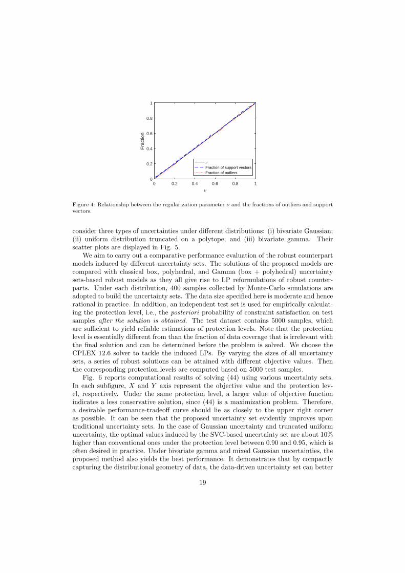
Next, we examine the validity of the established bounds for the fraction of outliersand support vectors, which are directly related to the conservatism and the complexityof the induced optimization problem. We calculate different fractions of outliers andsupport vectors by varying the value of ν, and the results are displayed in Fig. 4. Itcan be observed that the value of ν given by Propositions 3 and 4 manages to bound

16

-2 0 2 4 6 8

u(1)

-5

0

5

10

u(2)

(a) Box

-2 0 2 4 6 8

u(1)

-5

0

5

10

u(2)

(b) Ellipsoidal

-4 -2 0 2 4 6 8 10

u(1)

-10

-5

0

5

10

15

u(2)

(c) Polyhedral

Figure 2: Conventional uncertainty sets with data coverages of 99%, 90%, and 75%.

the fraction of outliers from above, and bound the fraction of support vectors frombelow. Notably, the gap between empirical performance and theoretical value is tight.It indicates that, the decision maker could conveniently control the conservatism of theinduced uncertainty set by adjusting the regularization parameter, while being aware ofthe complexity of robust counterpart formulation.

4.2. Optimization performance

Next, we conduct computational studies on the following robust LP problem underdifferent settings of uncertainty distributions.

maxx

8x1 + 2x2

s.t. (u1 + 5)x1 + (2 + u2)x2 ≤ 80

6x1 + 8x2 ≤ 200

x1, x2 ≥ 0

(44)

In this case, the uncertainties u = [u1 u2]T are postulated to affect the LHS of the firstconstraint only. In addition to the Gaussian mixture distribution adopted previously, we

17

(a) ν = 0.01 (b) ν = 0.05

(c) ν = 0.10 (d) ν = 0.15

(e) ν = 0.20 (f) ν = 0.25

Figure 3: Uncertainty sets construction based on different regularization parameter. Outliers residingoutside the uncertainty sets are marked as red diamonds.

18

0 0.2 0.4 0.6 0.8 1

ν

0

0.2

0.4

0.6

0.8

1

Fra

ctio

n

ν

Fraction of support vectorsFraction of outliers

Figure 4: Relationship between the regularization parameter ν and the fractions of outliers and supportvectors.

consider three types of uncertainties under different distributions: (i) bivariate Gaussian;(ii) uniform distribution truncated on a polytope; and (iii) bivariate gamma. Theirscatter plots are displayed in Fig. 5.

We aim to carry out a comparative performance evaluation of the robust counterpartmodels induced by different uncertainty sets. The solutions of the proposed models arecompared with classical box, polyhedral, and Gamma (box + polyhedral) uncertaintysets-based robust models as they all give rise to LP reformulations of robust counter-parts. Under each distribution, 400 samples collected by Monte-Carlo simulations areadopted to build the uncertainty sets. The data size specified here is moderate and hencerational in practice. In addition, an independent test set is used for empirically calculat-ing the protection level, i.e., the posteriori probability of constraint satisfaction on testsamples after the solution is obtained. The test dataset contains 5000 samples, whichare sufficient to yield reliable estimations of protection levels. Note that the protectionlevel is essentially different from than the fraction of data coverage that is irrelevant withthe final solution and can be determined before the problem is solved. We choose theCPLEX 12.6 solver to tackle the induced LPs. By varying the sizes of all uncertaintysets, a series of robust solutions can be attained with different objective values. Thenthe corresponding protection levels are computed based on 5000 test samples.

Fig. 6 reports computational results of solving (44) using various uncertainty sets.In each subfigure, X and Y axis represent the objective value and the protection lev-el, respectively. Under the same protection level, a larger value of objective functionindicates a less conservative solution, since (44) is a maximization problem. Therefore,a desirable performance-tradeoff curve should lie as closely to the upper right corneras possible. It can be seen that the proposed uncertainty set evidently improves upontraditional uncertainty sets. In the case of Gaussian uncertainty and truncated uniformuncertainty, the optimal values induced by the SVC-based uncertainty set are about 10%higher than conventional ones under the protection level between 0.90 and 0.95, which isoften desired in practice. Under bivariate gamma and mixed Gaussian uncertainties, theproposed method also yields the best performance. It demonstrates that by compactlycapturing the distributional geometry of data, the data-driven uncertainty set can better

19

hedge against uncertainties and help reducing the conservatism of solutions of robustoptimization.

The third row of Table 1 presents CPU times for solving robust counterpart LPs withdifferent ν used. Although the computational time grows with the increase of ν and moresupport vectors penetrating the robust counterpart problem, in all cases the induced LPcan be solved almost instantaneously in comparison with QPs for modeling uncertaintysets. This is due to an LP reformulation of the robust counterpart problem that can beefficiently tackled.

-6 -4 -2 0 2 4 6-6

-4

-2

0

2

4

6

(a) Gaussian

-4 -3 -2 -1 0 1 2 3-3

-2

-1

0

1

2

3

(b) Truncated uniform

-2 -1 0 1 2 3 4 5-5

-4

-3

-2

-1

0

1

2

3

4

(c) Bivariate gamma

-2 0 2 4 6 8-5

0

5

10

(d) Mixed Gaussian

Figure 5: Uncertainty data under different distributions.

The previous problem (44) only contains uncertainties on its LHS. It is worth men-tioning that the proposed uncertainty set and the associated robust counterpart are alsoapplicable to RHS uncertainties. Consider the following problem with uncertainties inboth LHS and RHS:

maxx

8x1 + 2x2

s.t. (u1 + 5)x1 + 2x2 ≤ 80− 7u2

6x1 + 8x2 ≤ 200

x1, x2 ≥ 0

(45)

20

70 80 90 100 110

Objective Value

0.65

0.7

0.75

0.8

0.85

0.9

0.95

1

Pro

tect

ion

Leve

l

SVCPolyhedralGammaBox

(a) Gaussian

75 80 85 90 95 100 105 110 115

Objective Value

0.65

0.7

0.75

0.8

0.85

0.9

0.95

1

Pro

tect

ion

Leve

l

SVCPolyhedralGammaBox

(b) Truncated uniform

65 70 75 80 85 90 95 100 105

Objective Value

0.65

0.7

0.75

0.8

0.85

0.9

0.95

1

Pro

tect

ion

Leve

l

SVCPolyhedralGammaBox

(c) Bivariate gamma

65 70 75 80 85 90 95 100 105

Objective Value

0.65

0.7

0.75

0.8

0.85

0.9

0.95

1

Pro

tect

ion

Leve

l

SVCPolyhedralGammaBox

(d) Mixed Gaussian

Figure 6: Results of robust optimization models under different uncertainties in LHS.

21

which can be handled by introducing an extra auxiliary decision variable x(3):

maxx

8x1 + 2x2

s.t. (u1 + 5)x1 + 2x2 + u2x3 ≤ 80

6x1 + 8x2 ≤ 200

x3 = 7

x1, x2 ≥ 0

(46)

The corresponding optimization results are reported in Fig. 7. Under the Gaussian andbivariate gamma uncertainties, the proposed uncertainty set induces the best perfor-mance, while in other cases its performance is comparable with conventional uncertaintysets.

85 90 95 100 105 110 115

Objective Value

0.75

0.8

0.85

0.9

0.95

1

Pro

tect

ion

Leve

l

SVCPolyhedralGammaBox

(a) Gaussian

95 100 105 110 115

Objective Value

0.75

0.8

0.85

0.9

0.95

1

Pro

tect

ion

Leve

l

SVCPolyhedralGammaBox

(b) Truncated uniform

78 80 82 84 86 88 90

Objective Value

0.75

0.8

0.85

0.9

0.95

1

Pro

tect

ion

Leve

l

SVCPolyhedralGammaBox

(c) Bivariate gamma

40 50 60 70 80

Objective Value

0.75

0.8

0.85

0.9

0.95

1

Pro

tect

ion

Leve

l

SVCPolyhedralGammaBox

(d) Mixed Gaussian

Figure 7: Results of robust optimization models under different uncertainties in both LHS and RHS.

5. Application to Robust Planning of Chemical Process Networks Planning

In this section, we study the application of the proposed robust optimization frame-work to a multi-period process network planning problem. Chemical complexes are typ-ically erected with a number of interconnected processes and versatile chemicals, which

22

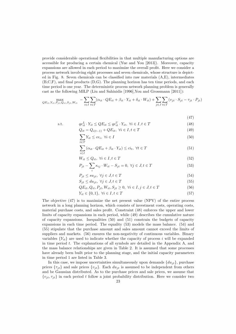
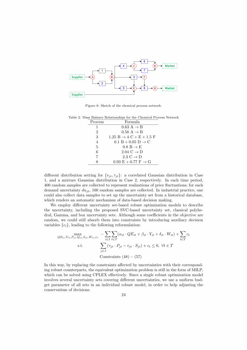
provide considerable operational flexibilities in that multiple manufacturing options areaccessible for producing a certain chemical (Yue and You [2013]). Moreover, capacityexpansions are allowed in each period to maximize the overall profit. Here we consider aprocess network involving eight processes and seven chemicals, whose structure is depict-ed in Fig. 8. Seven chemicals can be classified into raw materials (A,E), intermediates(B,C,F), and final products (D,G). The planning horizon has ten time periods, and eachtime period is one year. The deterministic process network planning problem is generallycast as the following MILP (Liu and Sahinidis [1996],You and Grossmann [2011]):

maxQEit,Yit,Pjt,Qit,Sjt,Wit

−∑i∈I

∑t∈T

(αit ·QEit + βit · Yit + δit ·Wit) +∑j∈J

∑t∈T

(vjt · Sjt − τjt · Pjt)

(47)

s.t. qeLit · Yit ≤ QEit ≤ qeUit · Yit, ∀i ∈ I, t ∈ T (48)

Qit = Qi(t−1) +QEit, ∀i ∈ I, t ∈ T (49)∑t∈T

Yit ≤ cei, ∀i ∈ I (50)∑i∈I

(αit ·QEit + βit · Yit) ≤ cit, ∀t ∈ T (51)

Wit ≤ Qit, ∀i ∈ I, t ∈ T (52)

Pjt −∑i

κij ·Wit − Sjt = 0, ∀j ∈ J, t ∈ T (53)

Pjt ≤ sujt, ∀j ∈ J, t ∈ T (54)

Sjt ≤ dujt, ∀j ∈ J, t ∈ T (55)

QEit, Qit, Pjt,Wit, Sjt ≥ 0, ∀i ∈ I, j ∈ J, t ∈ T (56)

Yit ∈ 0, 1, ∀i ∈ I, t ∈ T (57)

The objective (47) is to maximize the net present value (NPV) of the entire processnetwork in a long planning horizon, which consists of investment costs, operating costs,material purchase costs, and sales profit. Constraint (48) enforces the upper and lowerlimits of capacity expansions in each period, while (49) describes the cumulative natureof capacity expansions. Inequalities (50) and (51) constrain the budgets of capacityexpansions in each time period. The equality (53) models the mass balance. (54) and(55) stipulate that the purchase amount and sales amount cannot exceed the limits ofsuppliers and markets. (56) ensures the non-negativity of continuous variables. Binaryvariables Yit are used to indicate whether the capacity of process i will be expandedin time period t. The explanations of all symbols are detailed in the Appendix A, andthe mass balance relationships are given in Table 2. It is assumed that some processeshave already been built prior to the planning stage, and the initial capacity parametersin time period 1 are listed in Table 3.

In this case, we impose uncertainties simultaneously upon demands dujt, purchaseprices τjt and sale prices vjt. Each dujt is assumed to be independent from othersand be Gaussian distributed. As to the purchase prices and sale prices, we assume thatvjt, τjt in each period t follow a joint probability distribution. Here we consider two

23

Supplier A B

C D

E

F

G

1

2

3

4

5

6

7

8

Supplier

Market

Market

Figure 8: Sketch of the chemical process network.

Table 2: Mass Balance Relationships for the Chemical Process Network

Process Formula1 0.63 A→ B2 0.58 A→ B3 1.25 B→ 4 C + E + 1.5 F4 0.1 B + 0.05 D→ C5 0.8 B→ E6 2.04 C→ D7 2.3 C→ D8 0.93 E + 0.77 F→ G

different distribution setting for vjt, τjt: a correlated Gaussian distribution in Case1, and a mixture Gaussian distribution in Case 2, respectively. In each time period,400 random samples are collected to represent realizations of price fluctuations; for eachdemand uncertainty dujt, 100 random samples are collected. In industrial practice, onecould also collect data samples to set up the uncertainty set from a historical database,which renders an automatic mechanism of data-based decision making.

We employ different uncertainty set-based robust optimization models to describethe uncertainty, including the proposed SVC-based uncertainty set, classical polyhe-dral, Gamma, and box uncertainty sets. Although some coefficients in the objective arerandom, we could still absorb them into constraints by introducing auxiliary decisionvariables ct, leading to the following reformulation:

maxQEit,Yit,Pjt,Qit,Sjt,Wit,ct

−∑i∈I

∑t∈T

(αit ·QEit + βit · Yit + δit ·Wit) +∑t∈T

ct

s.t.∑j∈J

(τjt · Pjt − vjt · Sjt) + ct ≤ 0, ∀t ∈ T

Constraints (48)− (57)

In this way, by replacing the constraints affected by uncertainties with their correspond-ing robust counterparts, the equivalent optimization problem is still in the form of MILP,which can be solved using CPLEX effectively. Since a single robust optimization modelinvolves several uncertainty sets covering different uncertainties, we use a uniform bud-get parameter of all sets in an individual robust model, in order to help adjusting theconservatism of decisions.

24

Table 3: Initial Capacities of Processes

Process 1 2 3 4 5 6 7 8Capacity (kt/y) 0 40 180 400 0 30 0 120

Fig. 9 shows the performance comparisons of various robust optimization models indifferent uncertain environments. Under the same protection level, the proposed SVC-based uncertainty set gives the largest NPV value and hence enjoys the best performance.Then we make in-depth investigations into the solutions obtained under the correlatedGaussian uncertainties in Case 1. We adjust the budget parameters of different uncer-tainty sets such that the induced protection levels are almost the same (about 0.94),for the sake of reasonable comparisons. Due to the discrete nature of a finite numberof test samples, it may be impossible to have exactly identical protection levels. Theresulted solution statistics are summarized in Table 4. Note that the proposed SVC-based uncertainty set has the budget parameter value of ν = 0.16, which means thatthe uncertainty set contains at least 84% of available samples, thereby yielding a muchclearer interpretation than those of classical sets.

3.5 4 4.5 5 5.5

Objective Value ×105

0.65

0.7

0.75

0.8

0.85

0.9

0.95

1

Pro

tect

ion

Leve

l

SVCPolyhedralGammaBox

(a) Case 1: correlated Gaussian

1 2 3 4 5

Objective Value ×105

0.65

0.7

0.75

0.8

0.85

0.9

0.95

1

Pro

tect

ion

Leve

l

SVCPolyhedralGammaBox

(b) Case 2: mixture Gaussian

Figure 9: Robust planning performances of chemical process network.

Table 4: Comparisons of Solution Statistics between Robust Models based on Different Uncertainty Sets

SVC Polyhedral Gamma BoxMax. Profit ($) 470,420 441,130 442,930 454,150Protection Level 0.9392 0.9391 0.9391 0.9392

Budget Parameter ν = 0.16 Γ = 1.06 Γ = 1.08 Ψ = 0.58

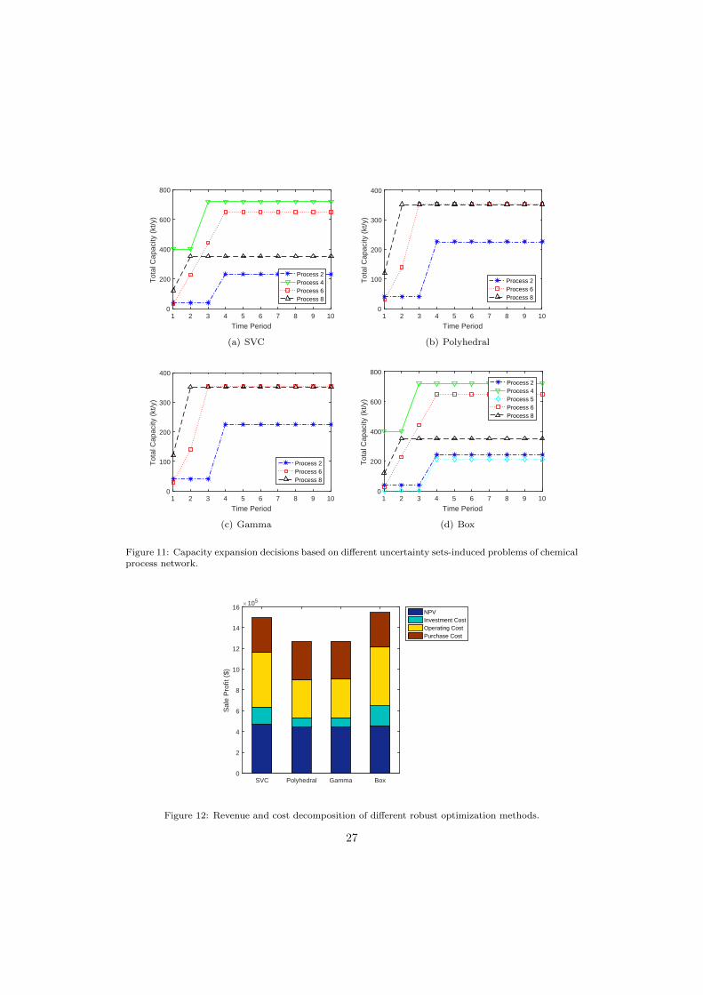
Next we compare tactical design and planning decisions made by models in Table4, and report the final results in Fig. 10. The box uncertainty set is shown to induceplanning configurations different from the others, in that the capacity of process 5 beingzero in time period 1 is expanded during the planning horizon. Then we further portraythe optimal capacity expansion strategies in Fig. 11. The decisions made based onpolyhedral and Gamma uncertainty sets only consider capacity expansions of processes

25

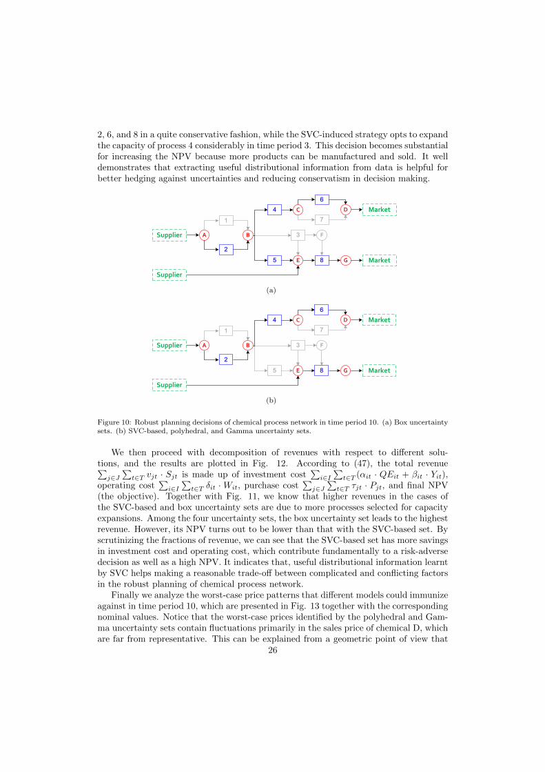
2, 6, and 8 in a quite conservative fashion, while the SVC-induced strategy opts to expandthe capacity of process 4 considerably in time period 3. This decision becomes substantialfor increasing the NPV because more products can be manufactured and sold. It welldemonstrates that extracting useful distributional information from data is helpful forbetter hedging against uncertainties and reducing conservatism in decision making.

Supplier A B

C D

E

F

G

1

2

3

4

5

6

7

8

Supplier

Market

Market

(a)

Supplier A B

C D

E

F

G

1

2

3

4

5

6

7

8

Supplier

Market

Market

(b)

Figure 10: Robust planning decisions of chemical process network in time period 10. (a) Box uncertaintysets. (b) SVC-based, polyhedral, and Gamma uncertainty sets.

We then proceed with decomposition of revenues with respect to different solu-tions, and the results are plotted in Fig. 12. According to (47), the total revenue∑j∈J

∑t∈T vjt · Sjt is made up of investment cost

∑i∈I∑t∈T (αit · QEit + βit · Yit),

operating cost∑i∈I∑t∈T δit ·Wit, purchase cost

∑j∈J

∑t∈T τjt · Pjt, and final NPV

(the objective). Together with Fig. 11, we know that higher revenues in the cases ofthe SVC-based and box uncertainty sets are due to more processes selected for capacityexpansions. Among the four uncertainty sets, the box uncertainty set leads to the highestrevenue. However, its NPV turns out to be lower than that with the SVC-based set. Byscrutinizing the fractions of revenue, we can see that the SVC-based set has more savingsin investment cost and operating cost, which contribute fundamentally to a risk-adversedecision as well as a high NPV. It indicates that, useful distributional information learntby SVC helps making a reasonable trade-off between complicated and conflicting factorsin the robust planning of chemical process network.

Finally we analyze the worst-case price patterns that different models could immunizeagainst in time period 10, which are presented in Fig. 13 together with the correspondingnominal values. Notice that the worst-case prices identified by the polyhedral and Gam-ma uncertainty sets contain fluctuations primarily in the sales price of chemical D, whichare far from representative. This can be explained from a geometric point of view that

26

1 2 3 4 5 6 7 8 9 10

Time Period

0

200

400

600

800

Tot

al C

apac

ity (

kt/y

)

Process 2Process 4Process 6Process 8

(a) SVC

1 2 3 4 5 6 7 8 9 10

Time Period

0

100

200

300

400

Tot

al C

apac

ity (

kt/y

)

Process 2Process 6Process 8

(b) Polyhedral

1 2 3 4 5 6 7 8 9 10

Time Period

0

100

200

300

400

Tot

al C

apac

ity (

kt/y

)

Process 2Process 6Process 8

(c) Gamma

1 2 3 4 5 6 7 8 9 10

Time Period

0

200

400

600

800T

otal

Cap

acity

(kt

/y)

Process 2Process 4Process 5Process 6Process 8

(d) Box

Figure 11: Capacity expansion decisions based on different uncertainty sets-induced problems of chemicalprocess network.

SVC Polyhedral Gamma Box0

2

4

6

8

10

12

14

16

Sal

e P

rofit

($)

×105

NPVInvestment CostOperating CostPurchase Cost

Figure 12: Revenue and cost decomposition of different robust optimization methods.

27

most extreme points of polyhedral and Gamma uncertainty sets lie exactly on the axis,and hence the worst-case perturbations tend to be sparse. As for the box uncertaintysets, the worst-case prices are pessimistic because both higher purchase prices and lowersales prices are considered. This is, however, still unrealistic since positive correlationsamong prices are assumed in Case 1. In contrast, the results obtained by the SVC-basedapproach are related to lower prices for all purchases and sales, which truthfully reflectsthe distributional information of uncertainties and hence enjoys greater rationality.

Purchasing A Purchasing E Selling D Selling G0

200

400

600

800

Wor

st-C

ase

Pric

e ($

/t)

NominalSVCPolyhedralGammaBox

Figure 13: The worst-case prices that different models immunize against at time period 10.

6. Concluding Remarks

In this work, we propose a novel data-driven uncertainty set based on piecewise linearkernel learning for solving robust optimization problems. We propose a new piecewiselinear kernel termed as the generalized intersection kernel, and integrate it with SVCfor effective unsupervised learning of convex data support. The SVC-based uncertaintyset inherits merits of nonparametric kernel learning methods, which could adapt to thecomplexity of data in an intelligent way. It allows the user to explicitly control the con-servatism as well as the complexity of robust optimization problems; most importantly,the induced robust counterpart problem can be formulated in the same type as the de-terministic problem, which enjoys computational tractability. Experimental results onnumerical optimization problems and an industrial application in chemical process net-work planning demonstrate that, by extracting meaningful information from data, theproposed data-driven robust optimization approach could better hedge against uncer-tainties, mitigate the over-conservatism, and improve the quality of robust solutions.

Future investigations can be considered in the following aspects. First, in the proposedscheme, the complexity of the induced robust counterpart problem is closely related to thepercentage of data coverage. One may want to further reduce the complexity while stillpreserving the fraction of data that are incorporated, especially when a large number oftraining samples are specified as outliers. This can be achieved by iteratively remodelingthe uncertainty set and excluding severe outliers, or by adopting disciplined techniquesin machine learning such as `1-norm regularization and Nystrom approximations.

Second, it is known that kernel methods tend to fall short of modeling high-dimensionaldata. In order to better deal with high-dimensional uncertainties, the proposed methodcan be further integrated with dimension reduction techniques such as PCA and ICA.

28

Acknowledgement

C. Shang and F. You acknowledge financial support from the National Science Foun-dation (NSF) CAREER Award (CBET-1643244). X. Huang is supported in part by theNational Natural Science Foundation of China under Grant 61603248.

Appendix A: Notations in Process Network Planning

Sets/indices

I set of processes indexed by i

J set of chemicals indexed by j

T set of time periods indexed by t

Parameters

cei maximum number of expansions for process i over the planning horizon

cit maximum allowable investment in time period t

djt demand of chemical j in time period t

sujt supply of chemical j in time period t

αit variable investment cost for process i in time period t

βit fixed investment cost for process i in time period t

δit unit operating cost for process i in time period t

τjt purchase price of chemical j in time period t

qeLit lower bound for capacity expansion of process i in time period t

qeUit upper bound for capacity expansion of process i in time period t

vjt sale price of chemical j in time period t

κij mass balance coefficient for chemical j in process i

Binary variables

Yit variable that indicates whether process i is expanded in time period t

Continuous variables

Pjt purchase amount of chemical j in time period t

Qit total capacity of process i in time period t

QEit capacity expansion of process i in time period t

Sjt sale amount of chemical j in time period t

Wit operation level of process i in time period t

29

References

Ben-Hur, A., Horn, D., Siegelmann, H.T., Vapnik, V., 2001. Support vector clustering. Journal ofMachine Learning Research 2, 125–137.

Ben-Tal, A., El Ghaoui, L., Nemirovski, A., 2009. Robust Optimization. Princeton University Press.Ben-Tal, A., Nemirovski, A., 1998. Robust convex optimization. Mathematics of Operations Research

23, 769–805.Ben-Tal, A., Nemirovski, A., 1999. Robust solutions of uncertain linear programs. Operations Research

Letters 25, 1–13.Ben-Tal, A., Nemirovski, A., 2000. Robust solutions of linear programming problems contaminated with

uncertain data. Mathematical Programming 88, 411–424.Bertsimas, D., Brown, D.B., Caramanis, C., 2011. Theory and applications of robust optimization.

SIAM Review 53, 464–501.Bertsimas, D., Gupta, V., Kallus, N., 2017. Data-driven robust optimization. Mathematical Program-

ming, 1–58, doi:10.1007/s10107-017-1125-8.Bertsimas, D., Pachamanova, D., 2008. Robust multiperiod portfolio management in the presence of

transaction costs. Computers & Operations Research 35, 3–17.Bertsimas, D., Sim, M., 2004. The price of robustness. Operations Research 52, 35–53.Birge, J.R., Louveaux, F., 2011. Introduction to Stochastic Programming. Springer Science & Business

Media.Bishop, C.M., 2006. Pattern Recognition and Machine Learning. Springer.Boyd, S., Vandenberghe, L., 2004. Convex Optimization. Cambridge University Press.Chen, X., Sim, M., Sun, P., 2007. A robust optimization perspective on stochastic programming.

Operations Research 55, 1058–1071.Delage, E., Ye, Y., 2010. Distributionally robust optimization under moment uncertainty with applica-

tion to data-driven problems. Operations Research 58, 595–612.El Ghaoui, L., Oustry, F., Lebret, H., 1998. Robust solutions to uncertain semidefinite programs. SIAM

Journal on Optimization 9, 33–52.Ferreira, R., Barroso, L., Carvalho, M., 2012. Demand response models with correlated price data: A

robust optimization approach. Applied Energy 96, 133–149.Gabrel, V., Murat, C., Thiele, A., 2014. Recent advances in robust optimization: An overview. European

Journal of Operational Research 235, 471–483.Gong, J., Garcia, D.J., You, F., 2016. Unraveling optimal biomass processing routes from bioconversion

product and process networks under uncertainty: An adaptive robust optimization approach. ACSSustainable Chemistry & Engineering 4, 3160–3173.

Gong, J., You, F., 2017. Optimal processing network design under uncertainty for producing fuelsand value-added bioproducts from microalgae: Two-stage adaptive robust mixed integer fractionalprogramming model and computationally efficient solution algorithm. AIChE Journal 63, 582–600.

Grant, M., Boyd, S., Ye, Y., 2008. CVX: Matlab software for disciplined convex programming.Guzman, Y.A., Matthews, L.R., Floudas, C.A., 2016. New a priori and a posteriori probabilistic bounds

for robust counterpart optimization: I. unknown probability distributions. Computers & ChemicalEngineering 84, 568–598.

Guzman, Y.A., Matthews, L.R., Floudas, C.A., 2017. New a priori and a posteriori probabilistic boundsfor robust counterpart optimization: II. a priori bounds for known symmetric and asymmetric prob-ability distributions. Computers & Chemical Engineering 101, 279–311.

Hanasusanto, G.A., Roitch, V., Kuhn, D., Wiesemann, W., 2017. Ambiguous joint chance constraintsunder mean and dispersion information. Operations Research 65, 751–767.

Huang, X., Suykens, J.A., Wang, S., Hornegger, J., Maier, A., 2017. Classification with truncated `1distance kernel. IEEE Transactions on Neural Networks and Learning Systems.

Hyvarinen, A., Karhunen, J., Oja, E., 2004. Independent Component Analysis. volume 46. John Wiley& Sons.

Jalilvand-Nejad, A., Shafaei, R., Shahriari, H., 2016. Robust optimization under correlated polyhedraluncertainty set. Computers & Industrial Engineering 92, 82–94.

Jiang, R., Guan, Y., 2016. Data-driven chance constrained stochastic program. Mathematical Program-ming 158, 291–327.

Kall, P., Wallace, S.W., Kall, P., 1994. Stochastic Programming. Springer.Lappas, N.H., Gounaris, C.E., 2016. Multi-stage adjustable robust optimization for process scheduling

under uncertainty. AIChE Journal .

30

Lee, J., Lee, D., 2005. An improved cluster labeling method for support vector clustering. IEEETransactions on Pattern Analysis and Machine Intelligence 27, 461–464.

Li, Z., Floudas, C.A., 2012. A comparative theoretical and computational study on robust counter-part optimization: II. probabilistic guarantees on constraint satisfaction. Industrial & EngineeringChemistry Research 51, 6769.

Liu, M.L., Sahinidis, N.V., 1996. Optimization in process planning under uncertainty. Industrial &Engineering Chemistry Research 35, 4154–4165.

Maji, S., Berg, A.C., Malik, J., 2008. Classification using intersection kernel support vector machines isefficient, in: IEEE Conference on Computer Vision and Pattern Recognition, pp. 1–8.

Maji, S., Berg, A.C., Malik, J., 2013. Efficient classification for additive kernel SVMs. IEEE Transactionson Pattern Analysis and Machine Intelligence 35, 66–77.

Muller, K.R., Mika, S., Ratsch, G., Tsuda, K., Scholkopf, B., 2001. An introduction to kernel-basedlearning algorithms. IEEE Transactions on Neural Networks 12, 181–201.

Mulvey, J.M., Vanderbei, R.J., Zenios, S.A., 1995. Robust optimization of large-scale systems. Opera-tions Research 43, 264–281.

Natarajan, K., Pachamanova, D., Sim, M., 2008. Incorporating asymmetric distributional informationin robust value-at-risk optimization. Management Science 54, 573–585.

Ning, C., You, F., 2017a. Data-driven adaptive nested robust optimization: General modeling frameworkand efficient computational algorithm for decision making under uncertainty. AIChE Journal, doi:10.1002/aic.15717.

Ning, C., You, F., 2017b. A data-driven multistage adaptive robust optimization framework for planningand scheduling under uncertainty. AIChE Journal, doi:10.1002/aic.15792.

Odone, F., Barla, A., Verri, A., 2005. Building kernels from binary strings for image matching. IEEETransactions on Image Processing 14, 169–180.

Pachamanova, D.A., 2002. A robust optimization approach to finance. Ph.D. thesis. MassachusettsInstitute of Technology.

Platt, J.C., 1999. Fast training of support vector machines using sequential minimal optimization.Advances in Kernel Methods , 185–208.

Qin, S.J., 2014. Process data analytics in the era of big data. AIChE Journal 60, 3092–3100.Sahinidis, N.V., 2004. Optimization under uncertainty: State-of-the-art and opportunities. Computers

& Chemical Engineering 28, 971–983.Scholkopf, B., Platt, J.C., Shawe-Taylor, J., Smola, A.J., Williamson, R.C., 2001. Estimating the support

of a high-dimensional distribution. Neural Computation 13, 1443–1471.Scholkopf, B., Smola, A.J., 2002. Learning with Kernels: Support Vector Machines, Regularization,

Optimization, and Beyond. MIT press.Scholkopf, B., Williamson, R.C., Smola, A.J., Shawe-Taylor, J., Platt, J.C., et al., 1999. Support vector

method for novelty detection., in: NIPS, pp. 582–588.Shi, H., You, F., 2016. A computational framework and solution algorithms for two-stage adaptive

robust scheduling of batch manufacturing processes under uncertainty. AIChE Journal 62, 687–703.Soyster, A.L., 1973. Technical noteconvex programming with set-inclusive constraints and applications

to inexact linear programming. Operations Research 21, 1154–1157.Suykens, J.A., Vandewalle, J., 1999. Least squares support vector machine classifiers. Neural Processing

Letters 9, 293–300.Tong, K., You, F., Rong, G., 2014. Robust design and operations of hydrocarbon biofuel supply chain

integrating with existing petroleum refineries considering unit cost objective. Computers & ChemicalEngineering 68, 128–139.

Vapnik, V., 2013. The Nature of Statistical Learning Theory. Springer Science & Business Media.You, F., Grossmann, I.E., 2011. Stochastic inventory management for tactical process planning under

uncertainties: MINLP models and algorithms. AIChE Journal 57, 1250–1277.Yuan, Y., Li, Z., Huang, B., 2015. Robust optimization approximation for joint chance constrained

optimization problem. Journal of Global Optimization , 1–23.Yuan, Y., Li, Z., Huang, B., 2016. Robust optimization under correlated uncertainty: Formulations and

computational study. Computers & Chemical Engineering 85, 58–71.Yue, D., You, F., 2013. Planning and scheduling of flexible process networks under uncertainty with

stochastic inventory: MINLP models and algorithm. AIChE Journal 59, 1511–1532.Yue, D., You, F., 2016. Optimal supply chain design and operations under multi-scale uncertainties:

Nested stochastic robust optimization modeling framework and solution algorithm. AIChE Journal62, 3041–3055.

Zymler, S., Kuhn, D., Rustem, B., 2013. Distributionally robust joint chance constraints with second-

31

order moment information. Mathematical Programming, 1–32.

32