Embed Size (px)
Citation preview

Data Analysis in Management with SPSS Software


J.P. Verma
Data Analysisin Managementwith SPSS Software

J.P. VermaResearch and Advanced StudiesLakshmibai National Universityof Physical Education
Gwalior, MP, India
ISBN 978-81-322-0785-6 ISBN 978-81-322-0786-3 (eBook)DOI 10.1007/978-81-322-0786-3Springer New Delhi Heidelberg New York Dordrecht London
Library of Congress Control Number: 2012954479
The IBM SPSS Statistics has been used in solving various applications in different chapters of the bookwith the permission of the International Business Machines Corporation, # SPSS, Inc., an IBMCompany. The various screen images of the software are Reprinted Courtesy of International BusinessMachines Corporation, # SPSS. “SPSS was acquired by IBM in October, 2009.”
IBM, the IBM logo, ibm.com, and SPSS are trademarks of International Business Machines Corp.,registered in many jurisdictions worldwide. Other product and service names might be trademarks ofIBM or other companies. A current list of IBM trademarks is available on theWeb at “IBMCopyright andtrademark information” at www.ibm.com/legal/copytrade.shtml.
# Springer India 2013This work is subject to copyright. All rights are reserved by the Publisher, whether the whole or partof the material is concerned, specifically the rights of translation, reprinting, reuse of illustrations,recitation, broadcasting, reproduction on microfilms or in any other physical way, and transmission orinformation storage and retrieval, electronic adaptation, computer software, or by similar or dissimilarmethodology now known or hereafter developed. Exempted from this legal reservation are brief excerptsin connection with reviews or scholarly analysis or material supplied specifically for the purpose of beingentered and executed on a computer system, for exclusive use by the purchaser of the work. Duplicationof this publication or parts thereof is permitted only under the provisions of the Copyright Law of thePublisher’s location, in its current version, and permission for use must always be obtained fromSpringer. Permissions for use may be obtained through RightsLink at the Copyright Clearance Center.Violations are liable to prosecution under the respective Copyright Law.The use of general descriptive names, registered names, trademarks, service marks, etc. in thispublication does not imply, even in the absence of a specific statement, that such names are exemptfrom the relevant protective laws and regulations and therefore free for general use.While the advice and information in this book are believed to be true and accurate at the date ofpublication, neither the authors nor the editors nor the publisher can accept any legal responsibility forany errors or omissions that may be made. The publisher makes no warranty, express or implied, withrespect to the material contained herein.
Printed on acid-free paper
Springer is part of Springer Science+Business Media (www.springer.com)

To my elder sister Sandhya Mohan forhaving me introduced in statisticsBrother-in-law Rohit Mohan for hishelping gestureAnd their angel daughter Saumya


Preface
While serving as a faculty of statistics for the last 30 years, I have experienced that
the non-statistics faculty and research scholars in different disciplines find it
difficult to use statistical techniques in their research problems. Even if their
theoretical concepts are sound its troublesome for them to use statistical software.
This book provides readers with a greater understanding of a variety of statistical
techniques along with the procedure to use the most popular statistical software
package SPSS.
The book strengthens the intuitive understanding of the material, thereby
increasing the ability to successfully analyze data in the future. It enhances readers
capability in using data analysis techniques to a broader spectrum of research
problems.
The book is intended for the undergraduate and postgraduate courses along with
pre-doctoral and doctoral course work on data analysis, statistics, and/or quantita-
tive methods taught in management and other allied disciplines like psychology,
economics, education, nursing, medical, or other behavioral and social sciences.
This book is equally useful to the advanced researchers in the area of humanities
and behavioural and social sciences in solving their research problems.
The book has been written to provide solutions to the researchers in different
disciplines for using one of the powerful statistical software SPSS. The book will
serve the students as a self-learning text of using SPSS for applying statistical
techniques in their research problems.
In most of the research studies, data are analyzed using multivariate statistics
which poses an additional problem for the beginners. These techniques cannot be
understood without in-depth knowledge of statistical concepts. Further, several
fields in science, engineering, and humanities have developed their own nomencla-
ture assigning different names to the same concepts. Thus, one has to gather
sufficient knowledge and experience in order to analyze their data efficiently.
This book covers most of the statistical techniques including some of the most
powerful multivariate techniques along with their detailed analysis and interpreta-
tion of the SPSS output that are required by the research scholars in different
discipline to achieve their research objectives.
vii
The USP of this book is that even without having the indepth knowledge of
statistics, one can learn various statistical techniques and their applications on their
own.
Each chapter is self-contained and starts with the topics like Introductory
concepts, application areas, statistical techniques used in the chapter and step-by-
step solved example with SPSS. In each chapter in depth interpretation of SPSS
output has been made to help the readers in understanding the application of
statistical techniques in different situations. Since the SPSS output generated in
different statistical applications are raw and cannot be directly used for reporting
hence model way of writing the results has been shown wherever it is required.
This book focuses on providing readers with the knowledge and skills needed to
carry out research in management, humanities, and social and behavioral sciences
by using SPSS. Looking at the contents and prospects of learning computing skills
using SPSS, this book is a must for every researcher from graduate-level studies
onward. Towards the end of each chapter, short answer questions, multiple-choice
questions, and assignments have been provided as a practice exercise for the readers.
The common mistakes like using two-tailed test for testing one-tailed hypothe-
sis, using the term “level of confidence” for defining level of significance or using
the statement like “accepting the null hypothesis” instead of “not able to reject the
null hypothesis” have been explained extensively in the text so that the readers may
avoid such mistakes during organizing and conducting their research work.
The faculty who uses this book will find it very useful as it presents many
illustrations with either real or simulated data to discuss analytical techniques in
different chapters. Some of the examples cited in the text are from my own and my
colleagues’ research studies.
This book consists of 14 chapters. Chapter 1 deals with the data types, data
cleaning, and procedure to start SPSS on the system. Notations used throughout the
book in using SPSS commands have been explained in this chapter. Chapter 2 deals
with descriptive study. Different situations have been discussed under which such
studies can be undertaken. The procedure of computing various descriptive statis-
tics has been discussed in this chapter. Besides computing procedure through SPSS,
a new approach has been shown towards the end of the second chapter to develop
the profile graph which can be used for comparing different domains of the
populations.
Chapter 3 explains the chi-square and its different applications by means of
solved examples. The step-by-step procedure of computing chi-square using SPSS
has been discussed. Chi-square is the test of significance for association between the
attributes, but it provides comparison of the two groups as well, in case of the
responses being measured on the nominal scale. This fact has been discussed for the
benefit of the readers.
Chapter 4 explains the procedure of computing correlation matrix and partial
correlations using SPSS. The emphasis has been given on how to interpret the
relationships.
In Chapter 5, computing multiple correlations and regression analysis have been
discussed. Both the approaches of regression analysis in SPSS i.e. Stepwise and
Enter methods have been discussed for estimating any measurable phenomenon.
viii Preface

In Chapter 6, application of t-test in testing the significance of difference
between groups in all the three situations, that is, in one sample, two independent
samples, and two dependent samples, has been discussed in detail. Procedures of
using one-tailed and two-tailed tests have been thoroughly detailed.
Chapter 7 explains the procedure of applying one-way analysis of variance
(ANOVA) with equal and unequal groups for testing the significance of variability
among group means. The graphical approach has been discussed for post hoc
comparisons of means besides using the p-value concept.In Chapter 8, two-way ANOVA for understanding the causes of variation has
been discussed in detail by means of solved examples using SPSS. The model way
of writing the results has been shown, which the students should note. Procedure for
doing interaction analysis has been discussed in detail by using the SPSS output.
In Chapter 9, the application of ANCOVA to study the role of covariate in
experimental research has been discussed by means of a research example. Students
can find the procedure of analyzing their data much easier after going through this
chapter.
In Chapter 10, cluster analysis technique has been discussed in detail for market
segmentation. The readers will come to know about the situations where cluster
analysis can be used in their research studies. Discussions of all its basic concepts
have been elaborated so that even a non-statistician can also appreciate and use it
for their research data.
Chapter 11 deals with the factor analysis, one of the most widely used multivari-
ate statistical techniques in management research. By going through this chapter,
the readers can understand to study the characteristics of a group of data by means
of few underlying structures instead of a large number of parameters. The proce-
dure of developing the test battery using the factor analysis technique has also been
discussed in detail.
In Chapter 12, we have discussed discriminant analysis and its application in
various research situations. By learning this technique, one can develop classifica-
tory model in classifying a customer into any of the two categories based on their
relevant profile parameters. The technique is very useful in classifying a customer
as good or bad for offering various services in the area of banking and insurance.
Chapter 13 explains the application of logistic regression for probabilistic
classification of cases into one of the two groups. Basics of this technique have
been discussed before explaining the procedure in solving logistic regression with
SPSS. Interpretations of each and every output have been very carefully explained
for easy understanding of the readers.
In Chapter 14, multidimensional scaling has been discussed to find the brand
positioning of different products. This technique is especially useful if the popular-
ity of products is to be compared on different parameters.
At each and every step, care has been taken so that the readers can learn to apply
SPSS and understand minutest possible detail of analysis discussed in this book.
The purpose of this book is to give a brief and clear description of how to apply
variety of statistical analysis using any version of SPSS. We hope that this book will
Preface ix

provide students and researchers with a self-learning material of using SPSS to
analyze their data.
Students and other readers are welcome to e-mail me their query related to any
portion of the book at [email protected], to which timely reply will be sent.
Professor (Statistics) J.P. Verma
x Preface

Acknowledgements
I would like to extend my sincere thanks to my professional colleagues
Prof. Y.P. Gupta, Prof. S. Sekhar, Dr. V.B. Singh, Prof. Jagdish Prasad and
Dr. J.P. Bhukar for their valuable inputs in completing this text. I must thank to
my research scholars who always motivated me to solve varieties of complex
research problems which has contributed a lot in preparing this text. Finally
I must appreciate the effort of my wife Hari Priya who not only provided me the
peaceful environment in preparing this text but also helped me in correcting
the manuscript language and format to a great extent. Finally I owe my loving
gesture to my children Prachi and Priyam who have provided me the creative inputs
in the preparation this manuscript.
Professor (Statistics) J.P. Verma
xi


Contents
1 Data Management . . . . . . . . . . . . . . . . . . . . . . . . . . . . . . . . . . . . . . 1
Introduction . . . . . . . . . . . . . . . . . . . . . . . . . . . . . . . . . . . . . . . . . . . 1
Types of Data . . . . . . . . . . . . . . . . . . . . . . . . . . . . . . . . . . . . . . . . . . 3
Metric Data . . . . . . . . . . . . . . . . . . . . . . . . . . . . . . . . . . . . . . . . . . 3
Nonmetric Data . . . . . . . . . . . . . . . . . . . . . . . . . . . . . . . . . . . . . . . 4
Important Definitions . . . . . . . . . . . . . . . . . . . . . . . . . . . . . . . . . . . . 5
Variable . . . . . . . . . . . . . . . . . . . . . . . . . . . . . . . . . . . . . . . . . . . . 5
Attribute . . . . . . . . . . . . . . . . . . . . . . . . . . . . . . . . . . . . . . . . . . . . 6
Mutually Exclusive Attributes . . . . . . . . . . . . . . . . . . . . . . . . . . . . 6
Independent Variable . . . . . . . . . . . . . . . . . . . . . . . . . . . . . . . . . . . 6
Dependent Variable . . . . . . . . . . . . . . . . . . . . . . . . . . . . . . . . . . . . 6
Extraneous Variable . . . . . . . . . . . . . . . . . . . . . . . . . . . . . . . . . . . 6
The Sources of Research Data . . . . . . . . . . . . . . . . . . . . . . . . . . . . . . 7
Primary Data . . . . . . . . . . . . . . . . . . . . . . . . . . . . . . . . . . . . . . . . . 7
Secondary Data . . . . . . . . . . . . . . . . . . . . . . . . . . . . . . . . . . . . . . . 9
Data Cleaning . . . . . . . . . . . . . . . . . . . . . . . . . . . . . . . . . . . . . . . . . . 9
Detection of Errors . . . . . . . . . . . . . . . . . . . . . . . . . . . . . . . . . . . . 10
Typographical Conventions Used in This Book . . . . . . . . . . . . . . . . . 11
How to Start SPSS . . . . . . . . . . . . . . . . . . . . . . . . . . . . . . . . . . . . . . 11
Preparing Data File . . . . . . . . . . . . . . . . . . . . . . . . . . . . . . . . . . . . . . 13
Defining Variables and Their Properties Under Different Columns . . 13
Defining Variables for the Data in Table 1.1 . . . . . . . . . . . . . . . . . . 16
Entering the Data . . . . . . . . . . . . . . . . . . . . . . . . . . . . . . . . . . . . . 16
Importing Data in SPSS . . . . . . . . . . . . . . . . . . . . . . . . . . . . . . . . . . 17
Importing Data from an ASCII File . . . . . . . . . . . . . . . . . . . . . . . . 18
Importing Data File from Excel Format . . . . . . . . . . . . . . . . . . . . . 22
Exercise . . . . . . . . . . . . . . . . . . . . . . . . . . . . . . . . . . . . . . . . . . . . . . 25
xiii

2 Descriptive Analysis . . . . . . . . . . . . . . . . . . . . . . . . . . . . . . . . . . . . 29
Introduction . . . . . . . . . . . . . . . . . . . . . . . . . . . . . . . . . . . . . . . . . . . 29
Measures of Central Tendency . . . . . . . . . . . . . . . . . . . . . . . . . . . . . . 31
Mean . . . . . . . . . . . . . . . . . . . . . . . . . . . . . . . . . . . . . . . . . . . . . . 31
Median . . . . . . . . . . . . . . . . . . . . . . . . . . . . . . . . . . . . . . . . . . . . . 36
Mode . . . . . . . . . . . . . . . . . . . . . . . . . . . . . . . . . . . . . . . . . . . . . . 38
Summary of When to Use the Mean, Median,
and Mode . . . . . . . . . . . . . . . . . . . . . . . . . . . . . . . . . . . . . . . . . . . 40
Measures of Variability . . . . . . . . . . . . . . . . . . . . . . . . . . . . . . . . . . . 41
The Range . . . . . . . . . . . . . . . . . . . . . . . . . . . . . . . . . . . . . . . . . . 41
The Interquartile Range . . . . . . . . . . . . . . . . . . . . . . . . . . . . . . . . . 41
The Standard Deviation . . . . . . . . . . . . . . . . . . . . . . . . . . . . . . . . . 42
Variance . . . . . . . . . . . . . . . . . . . . . . . . . . . . . . . . . . . . . . . . . . . . 45
The Index of Qualitative Variation . . . . . . . . . . . . . . . . . . . . . . . . . 46
Standard Error . . . . . . . . . . . . . . . . . . . . . . . . . . . . . . . . . . . . . . . . . 47
Coefficient of Variation (CV) . . . . . . . . . . . . . . . . . . . . . . . . . . . . . . 48
Moments . . . . . . . . . . . . . . . . . . . . . . . . . . . . . . . . . . . . . . . . . . . . . 49
Skewness . . . . . . . . . . . . . . . . . . . . . . . . . . . . . . . . . . . . . . . . . . . . . 50
Kurtosis . . . . . . . . . . . . . . . . . . . . . . . . . . . . . . . . . . . . . . . . . . . . . . 51
Percentiles . . . . . . . . . . . . . . . . . . . . . . . . . . . . . . . . . . . . . . . . . . . . 52
Percentile Rank . . . . . . . . . . . . . . . . . . . . . . . . . . . . . . . . . . . . . . . 53
Situation for Using Descriptive Study . . . . . . . . . . . . . . . . . . . . . . . . 53
Solved Example of Descriptive Statistics using SPSS . . . . . . . . . . . . . 54
Computation of Descriptive Statistics Using SPSS . . . . . . . . . . . . . 54
Interpretation of the Outputs . . . . . . . . . . . . . . . . . . . . . . . . . . . . . 58
Developing Profile Chart . . . . . . . . . . . . . . . . . . . . . . . . . . . . . . . . . . 62
Summary of the SPSS Commands . . . . . . . . . . . . . . . . . . . . . . . . . . . 63
Exercise . . . . . . . . . . . . . . . . . . . . . . . . . . . . . . . . . . . . . . . . . . . . . . 64
3 Chi-Square Test and Its Application . . . . . . . . . . . . . . . . . . . . . . . . 69
Introduction . . . . . . . . . . . . . . . . . . . . . . . . . . . . . . . . . . . . . . . . . . . 69
Advantages of Using Crosstabs . . . . . . . . . . . . . . . . . . . . . . . . . . . . . 70
Statistics Used in Cross Tabulations . . . . . . . . . . . . . . . . . . . . . . . . . . 70
Chi-Square Statistic . . . . . . . . . . . . . . . . . . . . . . . . . . . . . . . . . . . . 70
Chi-Square Test . . . . . . . . . . . . . . . . . . . . . . . . . . . . . . . . . . . . . . 72
Application of Chi-Square Test . . . . . . . . . . . . . . . . . . . . . . . . . . . 73
Contingency Coefficient . . . . . . . . . . . . . . . . . . . . . . . . . . . . . . . . 79
Lambda Coefficient . . . . . . . . . . . . . . . . . . . . . . . . . . . . . . . . . . . . 79
Phi Coefficient . . . . . . . . . . . . . . . . . . . . . . . . . . . . . . . . . . . . . . . 79
Gamma . . . . . . . . . . . . . . . . . . . . . . . . . . . . . . . . . . . . . . . . . . . . . 80
Cramer’s V . . . . . . . . . . . . . . . . . . . . . . . . . . . . . . . . . . . . . . . . . . 80
Kendall Tau . . . . . . . . . . . . . . . . . . . . . . . . . . . . . . . . . . . . . . . . . 80
Situation for Using Chi-Square . . . . . . . . . . . . . . . . . . . . . . . . . . . . . 80
Solved Examples of Chi-square for Testing an Equal
Occurrence Hypothesis . . . . . . . . . . . . . . . . . . . . . . . . . . . . . . . . . . . 81
xiv Contents
Computation of Chi-Square Using SPSS . . . . . . . . . . . . . . . . . . . . . 82
Interpretation of the Outputs . . . . . . . . . . . . . . . . . . . . . . . . . . . . . 84
Solved Examples of Chi-square for Testing the Significance
of Association Between Two Attributes . . . . . . . . . . . . . . . . . . . . . . . 87
Computation of Chi-Square for Two Variables
Using SPSS . . . . . . . . . . . . . . . . . . . . . . . . . . . . . . . . . . . . . . . . . . 88
Interpretation of the Outputs . . . . . . . . . . . . . . . . . . . . . . . . . . . . . 96
Summary of the SPSS Commands . . . . . . . . . . . . . . . . . . . . . . . . . . . 96
Exercise . . . . . . . . . . . . . . . . . . . . . . . . . . . . . . . . . . . . . . . . . . . . . . 98
4 Correlation Matrix and Partial Correlation: Explaining
Relationships . . . . . . . . . . . . . . . . . . . . . . . . . . . . . . . . . . . . . . . . . . 103
Introduction . . . . . . . . . . . . . . . . . . . . . . . . . . . . . . . . . . . . . . . . . . . 103
Details of Correlation Matrix and Partial Correlation . . . . . . . . . . . . . 105
Product Moment Correlation Coefficient . . . . . . . . . . . . . . . . . . . . . 106
Partial Correlation . . . . . . . . . . . . . . . . . . . . . . . . . . . . . . . . . . . . . 112
Situation for Using Correlation Matrix and Partial Correlation . . . . . . . 115
Research Hypotheses to Be Tested . . . . . . . . . . . . . . . . . . . . . . . . . 116
Statistical Test . . . . . . . . . . . . . . . . . . . . . . . . . . . . . . . . . . . . . . . . 117
Solved Example of Correlation Matrix and Partial Correlations by SPSS 117
Computation of Correlation Matrix Using SPSS . . . . . . . . . . . . . . . 118
Interpretation of the Outputs . . . . . . . . . . . . . . . . . . . . . . . . . . . . . 120
Computation of Partial Correlations Using SPSS . . . . . . . . . . . . . . . 123
Interpretation of Partial Correlation . . . . . . . . . . . . . . . . . . . . . . . . 125
Summary of the SPSS Commands . . . . . . . . . . . . . . . . . . . . . . . . . . . 126
Exercise . . . . . . . . . . . . . . . . . . . . . . . . . . . . . . . . . . . . . . . . . . . . . . 128
5 Regression Analysis and Multiple Correlations: For Estimating
a Measurable Phenomenon . . . . . . . . . . . . . . . . . . . . . . . . . . . . . . . 133
Introduction . . . . . . . . . . . . . . . . . . . . . . . . . . . . . . . . . . . . . . . . . . . 133
Terminologies Used in Regression Analysis . . . . . . . . . . . . . . . . . . . . 134
Multiple Correlation . . . . . . . . . . . . . . . . . . . . . . . . . . . . . . . . . . . 135
Coefficient of Determination . . . . . . . . . . . . . . . . . . . . . . . . . . . . . 137
The Regression Equation . . . . . . . . . . . . . . . . . . . . . . . . . . . . . . . . 138
Multiple Regression . . . . . . . . . . . . . . . . . . . . . . . . . . . . . . . . . . . 145
Application of Regression Analysis . . . . . . . . . . . . . . . . . . . . . . . . . . 149
Solved Example of Multiple Regression Analysis Including
Multiple Correlation . . . . . . . . . . . . . . . . . . . . . . . . . . . . . . . . . . . . . 149
Computation of Regression Coefficients, Multiple Correlation, and
Other Related Output in the Regression Analysis . . . . . . . . . . . . . . 150
Interpretation of the Outputs . . . . . . . . . . . . . . . . . . . . . . . . . . . . . 155
Summary of the SPSS Commands For Regression Analysis . . . . . . . . 159
Exercise . . . . . . . . . . . . . . . . . . . . . . . . . . . . . . . . . . . . . . . . . . . . . . 161
Contents xv

6 Hypothesis Testing for Decision-Making . . . . . . . . . . . . . . . . . . . . . 167
Introduction . . . . . . . . . . . . . . . . . . . . . . . . . . . . . . . . . . . . . . . . . . . 167
Hypothesis Construction . . . . . . . . . . . . . . . . . . . . . . . . . . . . . . . . . . 168
Null Hypothesis . . . . . . . . . . . . . . . . . . . . . . . . . . . . . . . . . . . . . . 170
Alternative Hypothesis . . . . . . . . . . . . . . . . . . . . . . . . . . . . . . . . . 170
Test Statistic . . . . . . . . . . . . . . . . . . . . . . . . . . . . . . . . . . . . . . . . . . . 170
Rejection Region . . . . . . . . . . . . . . . . . . . . . . . . . . . . . . . . . . . . . . . 171
Steps in Hypothesis Testing . . . . . . . . . . . . . . . . . . . . . . . . . . . . . . . . 171
Type I and Type II Errors . . . . . . . . . . . . . . . . . . . . . . . . . . . . . . . . . 172
One-Tailed and Two-Tailed Tests . . . . . . . . . . . . . . . . . . . . . . . . . . . 174
Criteria for Using One-Tailed and Two-Tailed Tests . . . . . . . . . . . . . . 175
Strategy in Testing One-Tailed and Two-Tailed Tests . . . . . . . . . . . . . 176
What Is p Value? . . . . . . . . . . . . . . . . . . . . . . . . . . . . . . . . . . . . . . . 177
Degrees of Freedom . . . . . . . . . . . . . . . . . . . . . . . . . . . . . . . . . . . . . 177
One-Sample t-Test . . . . . . . . . . . . . . . . . . . . . . . . . . . . . . . . . . . . . . 178
Application of One-Sample Test . . . . . . . . . . . . . . . . . . . . . . . . . . 179
Two-Sample t-Test for Unrelated Groups . . . . . . . . . . . . . . . . . . . . . . 181
Assumptions in Using Two-Sample t-Test . . . . . . . . . . . . . . . . . . . 181
Application of Two-Sampled t-Test . . . . . . . . . . . . . . . . . . . . . . . . 182
Assumptions in Using Paired t-Test . . . . . . . . . . . . . . . . . . . . . . . . 192
Testing Protocol in Using Paired t-Test . . . . . . . . . . . . . . . . . . . . . 192
Solved Example of Testing Single Group Mean . . . . . . . . . . . . . . . . . 196
Computation of t-Statistic and Related Outputs . . . . . . . . . . . . . . . . 196
Interpretation of the Outputs . . . . . . . . . . . . . . . . . . . . . . . . . . . . . 201
Solved Example of Two-Sample t-Test for Unrelated Groups with SPSS 201
Computation of Two-Sample t-Testfor Unrelated Groups . . . . . . . . . . . . . . . . . . . . . . . . . . . . . . . . . . . 202
Interpretation of the Outputs . . . . . . . . . . . . . . . . . . . . . . . . . . . . . 207
Solved Example of Paired t-Test with SPSS . . . . . . . . . . . . . . . . . . . . 208
Computation of Paired t-Test for Related Groups . . . . . . . . . . . . . . 209
Interpretation of the Outputs . . . . . . . . . . . . . . . . . . . . . . . . . . . . . 213
Summary of SPSS Commands for t-Tests . . . . . . . . . . . . . . . . . . . . . . 214
Exercise . . . . . . . . . . . . . . . . . . . . . . . . . . . . . . . . . . . . . . . . . . . . . . 215
7 One-Way ANOVA: Comparing Means of More
than Two Samples . . . . . . . . . . . . . . . . . . . . . . . . . . . . . . . . . . . . . . 221
Introduction . . . . . . . . . . . . . . . . . . . . . . . . . . . . . . . . . . . . . . . . . . . 221
Principles of ANOVA Experiment . . . . . . . . . . . . . . . . . . . . . . . . . . . 222
One-Way ANOVA . . . . . . . . . . . . . . . . . . . . . . . . . . . . . . . . . . . . 222
Factorial ANOVA . . . . . . . . . . . . . . . . . . . . . . . . . . . . . . . . . . . . . 223
Repeated Measure ANOVA . . . . . . . . . . . . . . . . . . . . . . . . . . . . . . 223
Multivariate ANOVA . . . . . . . . . . . . . . . . . . . . . . . . . . . . . . . . . . 224
One-Way ANOVA Model and Hypotheses Testing . . . . . . . . . . . . . . . 224
Assumptions in Using One-Way ANOVA . . . . . . . . . . . . . . . . . . . 228
Effect of Using Several t-tests Instead of ANOVA . . . . . . . . . . . . . . . 228
xvi Contents
Application of One-Way ANOVA . . . . . . . . . . . . . . . . . . . . . . . . . . . 229
Solved Example of One-Way ANOVA with Equal Sample Size Using
SPSS . . . . . . . . . . . . . . . . . . . . . . . . . . . . . . . . . . . . . . . . . . . . . . . . 233
Computations in One-Way ANOVA with Equal
Sample Size . . . . . . . . . . . . . . . . . . . . . . . . . . . . . . . . . . . . . . . . . 234
Interpretations of the Outputs . . . . . . . . . . . . . . . . . . . . . . . . . . . . . 238
Solved Example of One-Way ANOVA with Unequal Sample . . . . . . . 241
Computations in One-Way ANOVA with Unequal
Sample Size . . . . . . . . . . . . . . . . . . . . . . . . . . . . . . . . . . . . . . . . . 242
Interpretation of the Outputs . . . . . . . . . . . . . . . . . . . . . . . . . . . . . 246
Summary of the SPSS Commands for One-Way
ANOVA (Example 7.2) . . . . . . . . . . . . . . . . . . . . . . . . . . . . . . . . . . . 248
Exercise . . . . . . . . . . . . . . . . . . . . . . . . . . . . . . . . . . . . . . . . . . . . . . 249
8 Two-Way Analysis of Variance: Examining Influence
of Two Factors on Criterion Variable . . . . . . . . . . . . . . . . . . . . . . . 255
Introduction . . . . . . . . . . . . . . . . . . . . . . . . . . . . . . . . . . . . . . . . . . . 255
Principles of ANOVA Experiment . . . . . . . . . . . . . . . . . . . . . . . . . . . 256
Classification of ANOVA . . . . . . . . . . . . . . . . . . . . . . . . . . . . . . . . . 257
Factorial Analysis of Variance . . . . . . . . . . . . . . . . . . . . . . . . . . . . 257
Repeated Measure Analysis of Variance . . . . . . . . . . . . . . . . . . . . . 258
Multivariate Analysis of Variance (MANOVA) . . . . . . . . . . . . . . . 258
Advantages of Two-Way ANOVA over One-Way ANOVA . . . . . . . . 259
Important Terminologies Used in Two-Way ANOVA . . . . . . . . . . . . . 259
Factors . . . . . . . . . . . . . . . . . . . . . . . . . . . . . . . . . . . . . . . . . . . . . 259
Treatment Groups . . . . . . . . . . . . . . . . . . . . . . . . . . . . . . . . . . . . . 260
Main Effect . . . . . . . . . . . . . . . . . . . . . . . . . . . . . . . . . . . . . . . . . . 260
Interaction Effect . . . . . . . . . . . . . . . . . . . . . . . . . . . . . . . . . . . . . 260
Within-Group Variation . . . . . . . . . . . . . . . . . . . . . . . . . . . . . . . . . 260
Two-Way ANOVA Model and Hypotheses Testing . . . . . . . . . . . . . . 261
Assumptions in Two-Way Analysis of Variance . . . . . . . . . . . . . . . 265
Situation Where Two-Way ANOVA Can Be Used . . . . . . . . . . . . . . . 266
Solved Example of Two-Way ANOVA Using SPSS . . . . . . . . . . . . . . 272
Computation in Two-Way ANOVA Using SPSS . . . . . . . . . . . . . . . 273
Model Way of Writing the Results of Two-Way
ANOVA and Its Interpretations . . . . . . . . . . . . . . . . . . . . . . . . . . . 279
Summary of the SPSS Commands for Two-Way ANOVA . . . . . . . . . 285
Exercise . . . . . . . . . . . . . . . . . . . . . . . . . . . . . . . . . . . . . . . . . . . . . . 286
9 Analysis of Covariance: Increasing Precision in Comparison
by Controlling Covariate . . . . . . . . . . . . . . . . . . . . . . . . . . . . . . . . . 291
Introduction . . . . . . . . . . . . . . . . . . . . . . . . . . . . . . . . . . . . . . . . . . . 291
Introductory Concepts of ANCOVA . . . . . . . . . . . . . . . . . . . . . . . . . . 292
Graphical Explanation of Analysis of Covariance . . . . . . . . . . . . . . . . 293
Analysis of Covariance Model . . . . . . . . . . . . . . . . . . . . . . . . . . . . . . 294
Contents xvii

What We Do in Analysis of Covariance? . . . . . . . . . . . . . . . . . . . . . . 296
When to Use ANCOVA . . . . . . . . . . . . . . . . . . . . . . . . . . . . . . . . . . 297
Assumptions in ANCOVA . . . . . . . . . . . . . . . . . . . . . . . . . . . . . . . . . 298
Efficiency in Using ANCOVA over ANOVA . . . . . . . . . . . . . . . . . . . 298
Solved Example of ANCOVA Using SPSS . . . . . . . . . . . . . . . . . . . . 298
Computations in ANCOVA Using SPSS . . . . . . . . . . . . . . . . . . . . . 300
Model Way of Writing the Results of ANCOVA and Their
Interpretations . . . . . . . . . . . . . . . . . . . . . . . . . . . . . . . . . . . . . . . . . . 307
Summary of the SPSS Commands . . . . . . . . . . . . . . . . . . . . . . . . . . . 310
Exercise . . . . . . . . . . . . . . . . . . . . . . . . . . . . . . . . . . . . . . . . . . . . . . 311
10 Cluster Analysis: For Segmenting the Population . . . . . . . . . . . . . . 317
Introduction . . . . . . . . . . . . . . . . . . . . . . . . . . . . . . . . . . . . . . . . . . . 317
What Is Cluster Analysis? . . . . . . . . . . . . . . . . . . . . . . . . . . . . . . . . . 318
Terminologies Used in Cluster Analysis . . . . . . . . . . . . . . . . . . . . . . . 318
Distance Measure . . . . . . . . . . . . . . . . . . . . . . . . . . . . . . . . . . . . . 318
Clustering Procedure . . . . . . . . . . . . . . . . . . . . . . . . . . . . . . . . . . . 321
Standardizing the Variables . . . . . . . . . . . . . . . . . . . . . . . . . . . . . . 328
Icicle Plots . . . . . . . . . . . . . . . . . . . . . . . . . . . . . . . . . . . . . . . . . . 328
The Dendrogram . . . . . . . . . . . . . . . . . . . . . . . . . . . . . . . . . . . . . . 329
The Proximity Matrix . . . . . . . . . . . . . . . . . . . . . . . . . . . . . . . . . . 329
What We Do in Cluster Analysis . . . . . . . . . . . . . . . . . . . . . . . . . . . . 330
Assumptions in Cluster Analysis . . . . . . . . . . . . . . . . . . . . . . . . . . . . 331
Research Situations for Cluster Analysis Application . . . . . . . . . . . . . 332
Steps in Cluster Analysis . . . . . . . . . . . . . . . . . . . . . . . . . . . . . . . . . . 332
Solved Example of Cluster Analysis Using SPSS . . . . . . . . . . . . . . . . 333
Stage 1 . . . . . . . . . . . . . . . . . . . . . . . . . . . . . . . . . . . . . . . . . . . . . 335
Stage 2 . . . . . . . . . . . . . . . . . . . . . . . . . . . . . . . . . . . . . . . . . . . . . 335
Stage 1: SPSS Commands for Hierarchal
Cluster Analysis . . . . . . . . . . . . . . . . . . . . . . . . . . . . . . . . . . . . . . 335
Stage 2: SPSS Commands for K-Means
Cluster Analysis . . . . . . . . . . . . . . . . . . . . . . . . . . . . . . . . . . . . . . 340
Interpretations of Findings . . . . . . . . . . . . . . . . . . . . . . . . . . . . . . . 344
Exercise . . . . . . . . . . . . . . . . . . . . . . . . . . . . . . . . . . . . . . . . . . . . . . 354
11 Application of Factor Analysis: To Study the Factor
Structure Among Variables . . . . . . . . . . . . . . . . . . . . . . . . . . . . . . . 359
Introduction . . . . . . . . . . . . . . . . . . . . . . . . . . . . . . . . . . . . . . . . . . . 359
What Is Factor Analysis? . . . . . . . . . . . . . . . . . . . . . . . . . . . . . . . . . . 361
Terminologies Used in Factor Analysis . . . . . . . . . . . . . . . . . . . . . . . 361
Principal Component Analysis . . . . . . . . . . . . . . . . . . . . . . . . . . . . 362
Factor Loading . . . . . . . . . . . . . . . . . . . . . . . . . . . . . . . . . . . . . . . 362
Communality . . . . . . . . . . . . . . . . . . . . . . . . . . . . . . . . . . . . . . . . 362
Eigenvalues . . . . . . . . . . . . . . . . . . . . . . . . . . . . . . . . . . . . . . . . . 363
Kaiser Criteria . . . . . . . . . . . . . . . . . . . . . . . . . . . . . . . . . . . . . . . . 363
xviii Contents

The Scree Plot . . . . . . . . . . . . . . . . . . . . . . . . . . . . . . . . . . . . . . . . 363
Varimax Rotation . . . . . . . . . . . . . . . . . . . . . . . . . . . . . . . . . . . . . 364
What Do We Do in Factor Analysis? . . . . . . . . . . . . . . . . . . . . . . . . . 365
Assumptions in Factor Analysis . . . . . . . . . . . . . . . . . . . . . . . . . . . 366
Characteristics of Factor Analysis . . . . . . . . . . . . . . . . . . . . . . . . . 367
Limitations of Factor Analysis . . . . . . . . . . . . . . . . . . . . . . . . . . . . 367
Research Situations for Factor Analysis . . . . . . . . . . . . . . . . . . . . . . . 367
Solved Example of Factor Analysis Using SPSS . . . . . . . . . . . . . . . . . 368
SPSS Commands for the Factor Analysis . . . . . . . . . . . . . . . . . . . . 370
Interpretation of Various Outputs Generated
in Factor Analysis . . . . . . . . . . . . . . . . . . . . . . . . . . . . . . . . . . . . . 374
Summary of the SPSS Commands for Factor Analysis . . . . . . . . . . . . 381
Exercise . . . . . . . . . . . . . . . . . . . . . . . . . . . . . . . . . . . . . . . . . . . . . . 382
12 Application of Discriminant Analysis: For Developing
a Classification Model . . . . . . . . . . . . . . . . . . . . . . . . . . . . . . . . . . . 389
Introduction . . . . . . . . . . . . . . . . . . . . . . . . . . . . . . . . . . . . . . . . . . . 389
What Is Discriminant Analysis? . . . . . . . . . . . . . . . . . . . . . . . . . . . . . 390
Terminologies Used in Discriminant Analysis . . . . . . . . . . . . . . . . . . 391
Variables in the Analysis . . . . . . . . . . . . . . . . . . . . . . . . . . . . . . . . 391
Discriminant Function . . . . . . . . . . . . . . . . . . . . . . . . . . . . . . . . . . 392
Classification Matrix . . . . . . . . . . . . . . . . . . . . . . . . . . . . . . . . . . . 392
Stepwise Method of Discriminant Analysis . . . . . . . . . . . . . . . . . . . 392
Power of Discriminating Variables . . . . . . . . . . . . . . . . . . . . . . . . . 393
Box’s M Test . . . . . . . . . . . . . . . . . . . . . . . . . . . . . . . . . . . . . . . . 393
Eigenvalues . . . . . . . . . . . . . . . . . . . . . . . . . . . . . . . . . . . . . . . . . 393
The Canonical Correlation . . . . . . . . . . . . . . . . . . . . . . . . . . . . . . . 394
Wilks’ Lambda . . . . . . . . . . . . . . . . . . . . . . . . . . . . . . . . . . . . . . . 394
What We Do in Discriminant Analysis . . . . . . . . . . . . . . . . . . . . . . . . 394
Assumptions in Using Discriminant Analysis . . . . . . . . . . . . . . . . . 396
Research Situations for Discriminant Analysis . . . . . . . . . . . . . . . . . . 396
Solved Example of Discriminant Analysis Using SPSS . . . . . . . . . . . 397
SPSS Commands for Discriminant Analysis . . . . . . . . . . . . . . . . . . 399
Interpretation of Various Outputs Generated in Discriminant Analysis 403
Summary of the SPSS Commands for Discriminant Analysis . . . . . . . 407
Exercise . . . . . . . . . . . . . . . . . . . . . . . . . . . . . . . . . . . . . . . . . . . . . . 407
13 Logistic Regression: Developing a Model for Risk Analysis . . . . . . 413
Introduction . . . . . . . . . . . . . . . . . . . . . . . . . . . . . . . . . . . . . . . . . . . 413
What Is Logistic Regression? . . . . . . . . . . . . . . . . . . . . . . . . . . . . . . . 414
Important Terminologies in Logistic Regression . . . . . . . . . . . . . . . . . 415
Outcome Variable . . . . . . . . . . . . . . . . . . . . . . . . . . . . . . . . . . . . . 415
Natural Logarithms and the Exponent Function . . . . . . . . . . . . . . . . 415
Odds Ratio . . . . . . . . . . . . . . . . . . . . . . . . . . . . . . . . . . . . . . . . . . 416
Maximum Likelihood . . . . . . . . . . . . . . . . . . . . . . . . . . . . . . . . . . 416
Contents xix
Logit . . . . . . . . . . . . . . . . . . . . . . . . . . . . . . . . . . . . . . . . . . . . . . 417
Logistic Function . . . . . . . . . . . . . . . . . . . . . . . . . . . . . . . . . . . . . 417
Logistic Regression Equation . . . . . . . . . . . . . . . . . . . . . . . . . . . . . 417
Judging the Efficiency of the Logistic Model . . . . . . . . . . . . . . . . . 418
Understanding Logistic Regression . . . . . . . . . . . . . . . . . . . . . . . . . . 419
Graphical Explanation of Logistic Model . . . . . . . . . . . . . . . . . . . . 419
Logistic Model with Mathematical Equation . . . . . . . . . . . . . . . . . . 421
Interpreting the Logistic Function . . . . . . . . . . . . . . . . . . . . . . . . . . 422
Assumptions in Logistic Regression . . . . . . . . . . . . . . . . . . . . . . . . 423
Important Features of Logistic Regression . . . . . . . . . . . . . . . . . . . 423
Research Situations for Logistic Regression . . . . . . . . . . . . . . . . . . . . 424
Steps in Logistic Regression . . . . . . . . . . . . . . . . . . . . . . . . . . . . . . . 425
Solved Example of Logistics Analysis Using SPSS . . . . . . . . . . . . . . . 426
First Step . . . . . . . . . . . . . . . . . . . . . . . . . . . . . . . . . . . . . . . . . . . 427
Second Step . . . . . . . . . . . . . . . . . . . . . . . . . . . . . . . . . . . . . . . . . 428
SPSS Commands for the Logistic Regression . . . . . . . . . . . . . . . . . 428
Interpretation of Various Outputs Generated
in Logistic Regression . . . . . . . . . . . . . . . . . . . . . . . . . . . . . . . . . . 431
Explanation of Odds Ratios . . . . . . . . . . . . . . . . . . . . . . . . . . . . . . 437
Conclusion . . . . . . . . . . . . . . . . . . . . . . . . . . . . . . . . . . . . . . . . . . 437
Summary of the SPSS Commands for Logistic Regression . . . . . . . . . 437
Exercise . . . . . . . . . . . . . . . . . . . . . . . . . . . . . . . . . . . . . . . . . . . . . . 438
14 Multidimensional Scaling for Product Positioning . . . . . . . . . . . . . 443
Introduction . . . . . . . . . . . . . . . . . . . . . . . . . . . . . . . . . . . . . . . . . . . 443
What Is Multidimensional Scaling . . . . . . . . . . . . . . . . . . . . . . . . . . . 444
Terminologies Used in Multidimensional Scaling . . . . . . . . . . . . . . . . 444
Objects and Subjects . . . . . . . . . . . . . . . . . . . . . . . . . . . . . . . . . . . 444
Distances . . . . . . . . . . . . . . . . . . . . . . . . . . . . . . . . . . . . . . . . . . . 445
Similarity vs. Dissimilarity Matrices . . . . . . . . . . . . . . . . . . . . . . . . 445
Stress . . . . . . . . . . . . . . . . . . . . . . . . . . . . . . . . . . . . . . . . . . . . . . 445
Perceptual Mapping . . . . . . . . . . . . . . . . . . . . . . . . . . . . . . . . . . . . 445
Dimensions . . . . . . . . . . . . . . . . . . . . . . . . . . . . . . . . . . . . . . . . . . 446
What We Do in Multidimensional Scaling? . . . . . . . . . . . . . . . . . . . . 446
Procedure of Dissimilarity-Based Approach of Multidimensional
Scaling . . . . . . . . . . . . . . . . . . . . . . . . . . . . . . . . . . . . . . . . . . . . . 446
Procedure of Attribute-Based Approach of Multidimensional Scaling 447
Assumptions in Multidimensional Scaling . . . . . . . . . . . . . . . . . . . 448
Limitations of Multidimensional Scaling . . . . . . . . . . . . . . . . . . . . 449
Solved Example of Multidimensional Scaling
(Dissimilarity-Based Approach of Multidimensional Scaling)
Using SPSS . . . . . . . . . . . . . . . . . . . . . . . . . . . . . . . . . . . . . . . . . . . 449
xx Contents

SPSS Commands for Multidimensional Scaling . . . . . . . . . . . . . . . 450
Interpretation of Various Outputs Generated
in Multidimensional Scaling . . . . . . . . . . . . . . . . . . . . . . . . . . . . . 452
Summary of the SPSS Commands
for Multidimensional Scaling . . . . . . . . . . . . . . . . . . . . . . . . . . . . . . . 457
Exercise . . . . . . . . . . . . . . . . . . . . . . . . . . . . . . . . . . . . . . . . . . . . . . 457
Appendix: Tables . . . . . . . . . . . . . . . . . . . . . . . . . . . . . . . . . . . . . . . . . 461
References and Further Readings . . . . . . . . . . . . . . . . . . . . . . . . . . . . . 469
Index . . . . . . . . . . . . . . . . . . . . . . . . . . . . . . . . . . . . . . . . . . . . . . . . . . . 475
Contents xxi

Chapter 1
Data Management
Learning Objectives
After completing this chapter, you should be able to do the following:
• Explain different types of data generated in management research.
• Know the characteristics of variables.
• Learn to remove the outliers from the data by understanding different data
cleaning methods before using in SPSS.
• Understand the difference between primary and secondary data.
• Know the formats used in this book for using different commands,
subcommands, and options used in SPSS.
• Learn to install SPSS package for data analysis.
• Understand the procedure of importing data in other formats into SPSS.
• Prepare the data file for analysis in SPSS.
Introduction
In today’s world of information technology, enormous data is generated in every
organization. These data can help in strategic decision-making process. It is therefore
important to store such data in a warehouse so that effective mining can be done later
for getting answers to many of the management issues. Data warehousing and data
mining are therefore two important disciplines in the present-day scenario. Research
in any discipline is carried out in order to minimize inputs and effectively utilizing the
human resources, production techniques, governing principles, marketing policies,
and advertisement campaigns to maximize outputs in the form of productivity. To be
more specific, one may be interested to identify new forms of resources, devise
organizational systems and practices to motivate culturally diverse set of individuals,
and evaluate the existing organizations so as to make them more productive to the
new demands on them. Besides, there may be any number of other issues like
J.P. Verma, Data Analysis in Management with SPSS Software,DOI 10.1007/978-81-322-0786-3_1, # Springer India 2013
1

effective leadership, skill improvement, risk management, customer relationships,
and guiding the evolution of technology, etc., where the researcher can make an
effective contribution.
A researcher may use varieties of data analysis techniques in solving their
research problems like: How to motivate people for work? How to make a televi-
sion or FM channel more popular? How to enhance the productivity at work?
Which strategy becomes more efficient? How organizational structure promotes
innovation? How to measure training effectiveness? Due to cutthroat competition,
the research issues have grown in number, scope, and complexity over the years.
Due to availability of computer software for advanced data analysis, researcher has
become more eager to solve many of these complex issues.
The purpose of data analysis is to study the characteristics of sample data for
approximating it to the population characteristics. Drawing conclusion about the
population on the basis of sample would be valid only if the sample is true
representative of the population. This can be ensured by using the proper sampling
technique. However, large sample need not necessarily improves the efficiency in
findings. It is not the quantity but the quality of the sample that matters.
Data generated in management research may be analyzed by using different
kinds of statistical techniques. These techniques differ as per the nature of the study
which can be classified into any of the five categories; descriptive study, analytical
study, inductive study, inferential study and applied study. Choosing statistical
technique in data analysis depends upon nature of the problem. It is therefore
important to know the situation under which these techniques are used.
Descriptive study is used if an organization or a group of objects needs to be
studied about its different characteristics. In such studies, we usually tabulate and
compile the data in a meaningful manner so that the statistics like mean, variance,
standard error, coefficient of variance, range, skewness, kurtosis, percentiles, etc.,
can be computed in different groups.
Analytical studies are used for studying the functional relationships among
variables. Statistics like product moment correlation, partial and multiple
correlations are used in such study. Consider a study where it is required to explore
the parameters on which the sale depends. One may like to find correlation between
sales data and independent variables like incentives, salesman’s IQ, number of
marketing hours, and advertisement campaigns. Here, correlation between the sales
data and other parameters may be investigated for their significance. Thus, in all
those situations where relationships are investigated between the performance
parameter and other independent parameters, analytical studies are used.
Inductive studies are those studies which are used to estimate some phenomenon
of an individual or of an object on the basis of the sample data. Here, the
phenomenon which we estimate does not exist at the time of estimation. One may
estimate company’s performance in the next 3 years on the basis of some of its
present parameters like EPS, P/E ratio, cash reserves, demands, and production
capacity.
In inferential study, inferences are drawn about the population parameters on the
basis of sample data. Regression analysis is being used in such studies. The difference
2 1 Data Management

between inferential and inductive studies is that the phenomenon which we infer on
the basis of the sample exists in the inferential studies, whereas it is yet to occur in the
inductive studies. Thus, assessing satisfaction level in an organization on the basis of
a sample of employees may be the problem of inferential statistics.
Finally, applied studies refers to those studies which are used in solving the
problems of real life. The statistical methods such as times series analysis, index
numbers, quality control, and sample survey are included in this class of analysis.
Types of Data
Depending upon the data types, two broad categories of statistical techniques are
used for data analysis. For instance, parametric tests are used if the data are metric,
whereas in case of nonmetric data, nonparametric tests are used. It is therefore
important to know in advance the types of data which are generated in management
research.
Data can be classified in two categories, that is, metric and nonmetric. Metric and
nonmetric data are also known as quantitative and qualitative data, respectively.
Metric data is analyzed using parametric tests such as t, F, Z, and correlation coeffi-
cient, whereas nonparametric tests such as sign test, median test, chi-square test,
Mann-Whitney test, and Kruskal-Wallis test are used in analyzing nonmetric data.
Certain assumptions about the data and form of the distribution need to be satisfied
in using parametric tests. Parametric tests are more powerful in comparison to that of
nonparametric tests, provided required assumptions are satisfied. On the other hand,
nonparametric tests are more flexible and easy to use. Very few assumptions need to
be satisfied before using these tests. Nonparametric tests are also known as
distribution-free tests.
Let us understand the characteristics of different types of metric and nonmetric
data generated in research. Metric data is further classified into interval and ratio
data. On the other hand, nonmetric data is classified into nominal and ordinal. The
details of these four types of data are discussed below under two broad categories,
namely, metric data and nonmetric data, and are shown in Fig. 1.1.
Metric Data
Data is said to be metric if it is measured at least on interval scale. Metric data are
always associated with a scale measure, and, therefore, it is also known as scale data
or quantitative data. Metric data can be measured on two different types of scale,
that is, interval and ratio.
Types of Data 3

Interval Data
The interval data is measured along a scale where each position is equidistant from
one another. In this scale, the distance between two pairs is equivalent in some way.
In interval data, doubling principle breaks down as there is no zero on the scale. For
instance, the 6 marks given to an individual on the basis of his IQ do not explain that
his nature is twice as good as the person with 3 marks. Thus, interval variables
measured on an interval scale have values in which differences are uniform and
meaningful, but ratios are not. Interval data may be obtained if the parameters of job
satisfaction or level of frustration is rated on scale 1–10.
Ratio Data
The data on ratio scale has a meaningful zero value and has an equidistant measure
(i.e., the difference between 30 and 40 is the same as the difference between 60 and
70). For example, 60 marks obtained on a test are twice of 30. This is so because
zero can be measured on ratio scale. Ratio data can be multiplied and divided
because of an equidistant measure and doubling principle. Observations that we
measure or count are usually ratio data. Examples of ratio data are height, weight,
sales data, stock price, advance tax, etc.
Nonmetric Data
Nonmetric data is a categorical measurement and is expressed not in terms of
numbers but rather by means of a natural language description. It is often known
as “categorical” data. Examples of such data are like employee’s category ¼“executive,” department ¼ “production,” etc. These data can be measured on two
different scales, that is, nominal and ordinal.
Data Type
Metric data Non-metric data
Interval Ratio Nominal Ordinal
Fig. 1.1 Types of data and their classification
4 1 Data Management

Nominal Data
Nominal data is a categorical variable. These variables result from a selection in
categories. Examples might be employee’s status, industry types, subject speciali-
zation, race, etc. Data obtained on nominal scale is in terms of frequency. In SPSS,1
nominal data is represented as “nominal.”
Ordinal Data
Variables on the ordinal scale are also known as categorical variables, but here the
categories are ordered. The order of items is often defined by assigning numbers to
them to show their relative position. Categorical variables that assess performance
(good, average, poor, etc.) are ordinal variables. Similarly, attitudes (strongly agree,
agree, undecided, disagree, and strongly disagree) are also ordinal variables. On the
basis of the order of an ordinal variable, we may not know which value is the best or
worst on the measured phenomenon. Moreover, the distance between ordered
categories is also not measureable. No arithmetic can be done with the ordinal
data as they show sequence only. Data obtained on ordinal scale is in terms of ranks.
Ordinal data is denoted as “ordinal” in SPSS.
Important Definitions
Variable
A variable is a phenomenon that changes from time to time, place to place, and
individual to individual. Examples of variable are salary, scores in CAT examina-
tion, height, weight, etc. The variables can further be divided into discrete and
continuous. Discrete variables are those variables which can assume value from a
limited set of numbers. Examples of such variables are number of persons in a
department, number of retail outlets, number of bolts in a box, etc. On the other
hand, continuous variables can be defined as those variables that can take any valuewithin a range. Examples of such variables are height, weight, distance, etc.
1 SPSS, Inc. is an IBM company which was acquired by IBM in October, 2009.
Important Definitions 5

Attribute
An attribute can be defined as a qualitative characteristic that takes sub-values of a
variable, such as “male” and “female,” “student” and “teacher,” and married and
unmarried.
Mutually Exclusive Attributes
Attributes are said to be mutually exclusive if they cannot occur at the same time.
Thus, in a survey, a person can choose only one option from a list of alternatives (as
opposed to selecting as many that might apply). Similarly in choosing the gender,
one can either choose male or female.
Independent Variable
Any variable that can be manipulated by the researcher is known as independent
variable. In planning a research experiment, to see the effect of low, medium, and
high advertisement cost on sales performance, advertisement cost is an independent
variable as the researcher can manipulate it.
Dependent Variable
A variable is said to be dependent if it changes as a result of change in the
independent variable. In investigating the impact on sales performance by the
change in advertisement cost, the sales performance is a dependent variable,
whereas advertisement cost is an independent variable. In fact, a variable may be
a dependent variable in one study and independent variable in some other study.
Extraneous Variable
Any additional variable that may provide alternative explanations or cast doubt on
conclusions in an experimental study is known as extraneous variable. If the effect
of three different teaching methods on the student’s performance is to be compared,
then the IQ of the students may be termed as extraneous variable as it might affect
the learning efficiency during experimentation if the IQs are not same in all the
groups.
6 1 Data Management

The Sources of Research Data
In designing a research experiment, one needs to specify the kind of data required
and how to obtain it. The researcher may obtain the data from the reliable source if
it is available. But if the required data is not available from any source, it may
be collected by the researcher themselves. Several agencies collect data for some
specified purposes and make them available for the other researchers to draw
other meaningful conclusions as per their plan of study. Even some of the
commercial agencies provide the real-time data to the users with cost. The data
so obtained from other sources are referred as secondary data, whereas the data
collected by the researchers themselves are known as primary data. We shall now
discuss other features of these data in the following sections:
Primary Data
The data obtained during study by the researchers themselves or with the help
of their colleagues, subordinates, or field investigators are known as primary data.
The primary data is obtained by the researcher in a situation where relevant data
is not available from the reliable sources or such data do not exist with any of
the agency or if the study is an experimental study where specific treatments are
required to be given in the experiment. The primary data is much more reliable
because of the fact that the investigator himself is involved in data collection and
hence can ensure the correctness of the data. Different methods can be used to collect
the primary data by the researcher. These methods are explained below:
By Observation
The data in this method is obtained by observation. One can ensure the quality of
data as the investigator himself observes real situation and records the data.
For example, to assess the quality of any product, one can see as to how the
articles are prepared by the particular process. In an experimental study, the
performance of the subjects, their behavior, and other temperaments can be
noted after they have undergone a treatment. The drawback of this method is
that sometimes it becomes very frustrating for the investigator to be present all
the time for collecting the data. Further, if an experiment involves the human
being, then the subjects may become conscious in the presence of an investigator,
due to which performance may be affected which will ultimately result in
inaccurate data.
The Sources of Research Data 7

Through Surveys
This is the most widely used method of data collection in the area of management,
psychology, market research, and other behavioral studies. The researcher must try
to motivate respondents by explaining them the purpose of the survey and impact of
their responses on the results of the study. The questionnaire must be short and must
hide the identity of respondents. Further, the respondent may be provided reason-
able incentives as per the availability of the budget. For instance, a pen, a pencil, or
a notepad with print statements like “With best Compliments from. . .” or “With
Thanks. . .,” “Go Green,” “Save Environment” may be provided before seeking
their opinion on the questionnaire. You can print your organization name or your
name as well if you are an independent researcher. The first two slogans may
promote your company as well, whereas the other two convey the social message to
the respondents. The investigator must ensure the authenticity of the collected data
by means of cross-checking some of the sampled information.
From Interviews
The data collected through the direct interview allows the investigator to go for in-
depth questioning and follow-up questions. The method is slow and costly and
forces an individual to be away from the job during the time of interview. During
the interview, the respondent may provide the wrong information if certain sensi-
tive issues are touched upon, and the respondent may like to avoid it on the premise
that it might suffer their reputation. For instance, if the respondent’s salary is very
low and the questions are asked about his salary, it is more likely that you end up
with the wrong information. Similarly in asking the question, as to how much you
invest on sports for your children in a year, you might get wrong information due to
the false ego of respondent.
Through Logs
The data obtained through the logs maintained by the organizations may be used as
primary data. Fault logs, error logs, complaint logs, and transaction logs may be
used to extract the required data for the study. Such data provide valuable findings
about system performance over time under different conditions if used well, as they
are empirical data and obtained from the objective data sources.
Primary data can be considered to be reliable because you know how it was
collected and what was done to it. It is something like cooking yourself. You know
what went into it.
8 1 Data Management

Secondary Data
Instead of data obtained by the investigator himself if it is obtained from some other
sources, it is termed as secondary data. Usually, companies collect the data for some
specific purpose, and after that, they publish it for the use of the researchers to draw
some meaningful conclusions as per their requirements. Many government
agencies allow their real-time data to the researchers for using in their research
study. For instance, census data collected by the National Sample Surveys Organi-
zation may be used by the researchers for getting several demographic and socio-
economic information. Government departments and universities maintain their
open-source data and allow the researchers to use it. Nowadays, many commercial
agencies collect the data in different fields and make it available to the researchers
with nominal cost.
The secondary data may be obtained from many sources; some of them are listed
below:
• Government ministries through national informatics center
• Government departments
• Universities
• Thesis and research reports
• Open-source data
• Commercial organization
Care must be taken to ensure the reliability of the agency from which the data is
obtained. One must ensure to take an approval of the concerned department,
agency, organization, universities, or individuals for using their data. Due acknowl-
edgment must be shown in their research report for using their data. Further, data
source must be mentioned while using the data obtained from secondary sources.
In making comparison between primary and secondary data, one may conclude
that primary data is expensive and difficult to acquire, but it is more reliable.
Secondary data is cheap and easy to collect but must be used with caution.
Data Cleaning
Before preparing the data file for analysis, it is important to organize the data on
paper first. There are more chances that the data set may contain error or outlier.
And if it is so, the results obtained may be erroneous. Analysts tend to waste lot of
time in drawing the valid conclusions if data is erroneous. Thus, it is utmost
important that the data must be cleaned before analysis. If data is clean, the analysis
is straightforward and valid conclusions may be drawn.
Data Cleaning 9
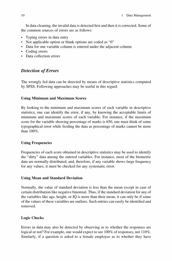
In data cleaning, the invalid data is detected first and then it is corrected. Some of
the common sources of errors are as follows:
• Typing errors in data entry
• Not applicable option or blank options are coded as “0”
• Data for one variable column is entered under the adjacent column
• Coding errors
• Data collection errors
Detection of Errors
The wrongly fed data can be detected by means of descriptive statistics computed
by SPSS. Following approaches may be useful in this regard.
Using Minimum and Maximum Scores
By looking to the minimum and maximum scores of each variable in descriptive
statistics, one can identify the error, if any, by knowing the acceptable limits of
minimum and maximum scores of each variable. For instance, if the maximum
score for the variable showing percentage of marks is 650, one must think of some
typographical error while feeding the data as percentage of marks cannot be more
than 100%.
Using Frequencies
Frequencies of each score obtained in descriptive statistics may be used to identify
the “dirty” data among the entered variables. For instance, most of the biometric
data are normally distributed, and, therefore, if any variable shows large frequency
for any values, it must be checked for any systematic error.
Using Mean and Standard Deviation
Normally, the value of standard deviation is less than the mean except in case of
certain distribution like negative binomial. Thus, if the standard deviation for any of
the variables like age, height, or IQ is more than their mean, it can only be if some
of the values of these variables are outliers. Such entries can easily be identified and
removed.
Logic Checks
Errors in data may also be detected by observing as to whether the responses are
logical or not? For example, one would expect to see 100% of responses, not 110%.
Similarly, if a question is asked to a female employee as to whether they have
10 1 Data Management
availed maternity leave so far or not and if the reply is marked “yes” but you notice
that the respondent is coded as male, such logical errors can be spotted out by
looking to the values of the categorical variable. Logical approach should be used
judiciously to avoid the embarrassing situation in reporting the finding like 10% of
the men in the sample had availed the maternity leave during the last 10 years.
Typographical Conventions Used in This Book
Throughout the book, certain convention has been followed in writing commands
by means of symbol, bold words, italic words, and words in quotes to signify the
special meaning. Readers should note these conventions for easy understanding of
commands used in different chapters of this book.
Start ⟹ All
Programs
Denotes a menu command, which means choosing the command All
Program from the Start menu. Similarly Analyze ⟹ Correlate ⟹Partial means open the Analyze menu, then open the Correlate
submenu, and finally choose Partial.
Regression Any word written in bold refers to the main command of any window in the
SPSS package.
Prod_Data Any word or combination of words written in italics form during explaining
SPSS is referred as variable.
“Name” Any word or combination of words written in quotes refers to the
subcommand.
‘Scale’ Any word written in single quote refers to one of the option under
subcommand.
Continue This refers to the end of selection of commands in a window and will take
you to the next level of options in any computation.
OK This refers to the end of selecting all the options required for any particular
analysis. After pressing the OK invariably, SPSS will lead you to the
output window.
How to Start SPSS
This book has been written by referring to the IBM SPSS Statistics 20.0 version;
however, in all the previous versions of SPSS, procedure of computing is more or
less similar.
The SPSS needs to be activated on your computer before entering the data. This
can be done by clicking the left button of the mouse on SPSS tag by going through
the SPSS directory in the Start and All Programs option (if the SPSS directory has
been created in the Programs file). Using the following command sequence, SPSS
can be activated on your computer system:
How to Start SPSS 11
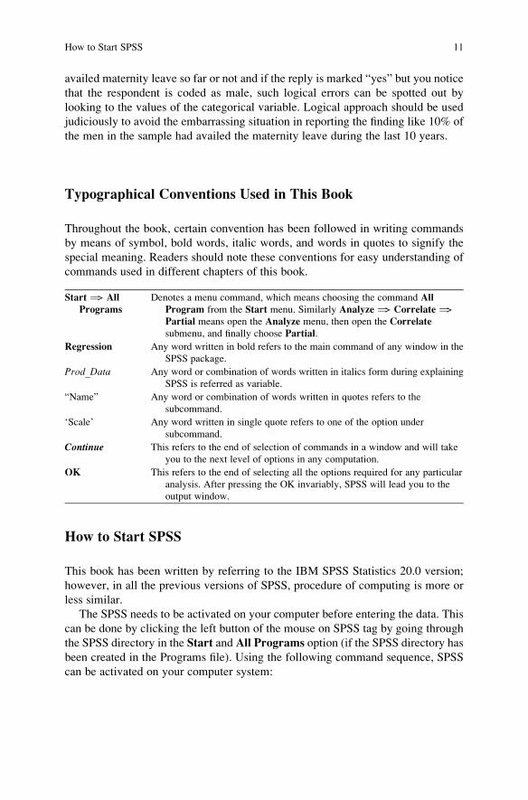
Start ! All Programs ! IBM SPSS Statistics ! IBM SPSS Statistics 19
If you use the above-mentioned command sequence, the screen shall look like
Fig. 1.2.
After clicking the tag SPSS, you will get the following screen to prepare the data
file or open the existing data file.
If you are entering the data for new problem and the file is to be created for the
first time, check the following option in the above-mentioned window:
And if the existing file is to be opened or edited, select the following option in
the window:
Fig. 1.2 Commands for starting SPSS on your computer
12 1 Data Management

Click OK to get the screen to define the variables in the Variable View. Details
of preparing data file are shown below.
Preparing Data File
The procedure of preparing the data file shall be explained by means of the data
shown in Table 1.1.
In SPSS, before entering data, all the variables need to be defined in the
Variable View. Once Type in data option is selected in the screen shown in
Fig. 1.3, click the Variable View. This will allow you to define all the variables
in the SPSS. The blank screen shall look like Fig. 1.4.
Now you are ready for defining the variables row wise.
Defining Variables and Their Properties Under Different Columns
Column 1: In first column, short name of the variables are defined. The variable
name should essentially start with an alphabet and may use under-
score and numerals in between, without any gap. There should be no
space between any two characters of the variable name. Further,
variable name should not be started with numerals or any special
character.
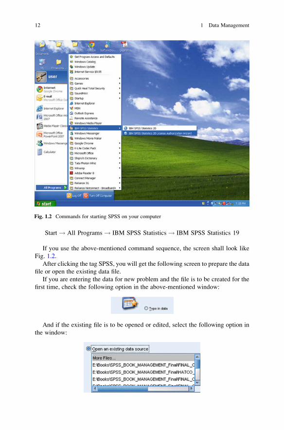
Column 2: Under the column heading “Type,” format of the variable (numeric or
nonnumeric) and the number of digits before and after decimal are
defined. This can be done by double-clicking the concerned cell. The
screen shall look like Fig. 1.5.
Table 1.1 FDI inflows and
trade (in percent) in different
states
S.N. FDI Exports inflows Imports Trade
1 4.92 4.03 3.12 3.49
2 0.07 4.03 3.12 3.49
3 0.00 1.11 2.69 2.04
4 5.13 17.11 27.24 23.07
5 11.14 13.43 11.24 12.14
6 0.48 1.14 3.41 2.47
7 0.30 2.18 1.60 1.84
8 29.34 20.56 18.68 19.45
9 0.57 1.84 1.16 1.44
10 0.03 1.90 1.03 1.39
11 8.63 5.24 9.24 7.59
12 0.00 3.88 6.51 5.43
13 2.20 7.66 1.57 4.08
14 2.37 4.04 4.76 4.46
15 34.01 14.53 3.35 7.95
16 0.81 1.00 1.03 1.02
Preparing Data File 13

Column 3: Under the column heading “Width,” number of digits a variable can
have may be altered.
Column 4: In this column, number of decimal a variable can have may be altered.
Column 5: Under the column heading “Label,” full name of the variable can be
defined. The user can take advantage of this facility to write the
expanded name of the variable the way one feels like.
Fig. 1.3 Screen showing the option for creating/opening file
Fig. 1.4 Blank format for defining the variables in SPSS
14 1 Data Management
Column 6: Under the column heading “Values,” the coding of the variable may
be defined by double clicking the cell. Sometimes, the variable is of
classificatory in nature. For example, if there is a choice of choosing
any one of the following four departments for training
(a) Production
(b) Marketing
(c) Human resource
(d) Public relation
then these departments can be coded as 1 ¼ production, 2 ¼ market-
ing, 3¼ human resource, and 4¼ public relation. While entering data
into the computer, these codes are entered, as per the response of a
particular subject. SPSS window showing the option for entering code
has been shown in Fig. 1.6.
Column 7: In survey study, it is quite likely that for certain questions the respon-
dent does not reply, which creates the problem of missing value. Such
missing value can be defined under column heading “Missing.”
Column 8: Under the heading “Columns,” width of the column space where data
is typed in Data View is defined.
Column 9: Under the column heading “Align,” the alignment of data while
feeding may be defined as left, right, or center.
Column 10: Under the column heading “Measure,” the variable type may be
defined as scale, ordinal, or nominal.
Fig. 1.5 Option showing defining of variable as numeric or nonnumeric
Preparing Data File 15

Defining Variables for the Data in Table 1.1
1. Write short name of all the five variables as States, FDI_Inf, Export, Import, andTrade under the column heading “Name.”
2. Under the column heading “Label,” full name of these variables may be defined
as FDI Inflows, Export Data, Import Data, and Trade Data. One can take libertyof defining some more detailed name of these variables as well.
3. Use default entries in rest of the columns.
After defining variables in the variable view, the screen shall look like Fig. 1.7.
Entering the Data
After defining all the five variables in the Variable View, click Data View on the
left bottom of the screen to open the format for entering the data. For each variable,
data can be entered column wise. After entering the data, the screen will look like
Fig. 1.8. Save the data file in the desired location before further processing.
After preparing the data file, one may use different types of statistical analysis
available under the tag Analyze in the SPSS package. Different types of statistical
analyses have been discussed in different chapters of the book along with their
interpretations. Methods of data entry are different in certain applications; for
Fig. 1.6 Screen showing how to define the code for the different labels of the variable
16 1 Data Management

instance, readers are advised to note carefully the way data is entered for the
application in Example 6.2 in Chap. 6. Relevant details have been discussed in
that chapter.
Importing Data in SPSS
In SPSS, data can be imported from ASCII as well as Excel file. The procedure of
importing these two types of data files has been discussed in the following sections.
Fig. 1.8 Screen showing entered data for all the variables in the data view
Fig. 1.7 Variables along with their characteristics for the data shown in Table 1.1
Importing Data in SPSS 17

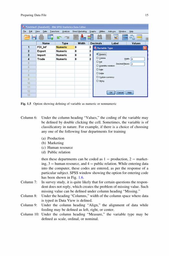
Importing Data from an ASCII File
In ASCII file, data for each variable may be separated by a space, tab, comma, or
some other character. The Text Import Wizard in SPSS facilitates you to import
data from an ASCII file format. Consider the following set of data in ASCII file
saved on the desktop by the file name Business data:
File name: Business data
S.N. FDI Exports inflows Imports Trade
1 4.92 4.03 3.12 3.49
2 0.07 4.03 3.12 3.49
3 0.00 1.11 2.69 2.04
4 5.13 17.11 27.24 23.07
5 11.14 13.43 11.24 12.14
The sequence of commands is as follows:
1. For importing the required ASCII file into SPSS, follow the below-mentioned
sequence of commands in Data View.
File�> Open�>Data�> Businessdata
– Choose “Text” as the “File Type” if your ASCII file has the .txt extension.
Otherwise, choose the option “All files.”
– After selecting the file that you want to import, click Open as shown in
Fig. 1.9.
2. After choosing the ASCII file from the saved location in Fig. 1.9, the Text Import
Wizard will pop up automatically as shown in Fig. 1.10 that will take you for
further option in importing the file. Take the following steps:
– If your file does not match a predefined format, which is usually not, so click
Next.
3. After clicking the Next option above, you will get the screen as shown in
Fig. 1.11. Take the following steps:
– Define delimiter and check the option “Delimited” as the data in the file is
separated by either space or comma.
– If variable names are written in the first row of your data file, check the header
row option as “Yes,” otherwise “No.” In this, the option “Yes” will be
selected because variable names have been written in the first row of the
data file. Click Next.
4. After clicking the option Next, you will get the screen as shown in Fig. 1.12.
Enter the line number where the first case of your data begins. If there is no
18 1 Data Management
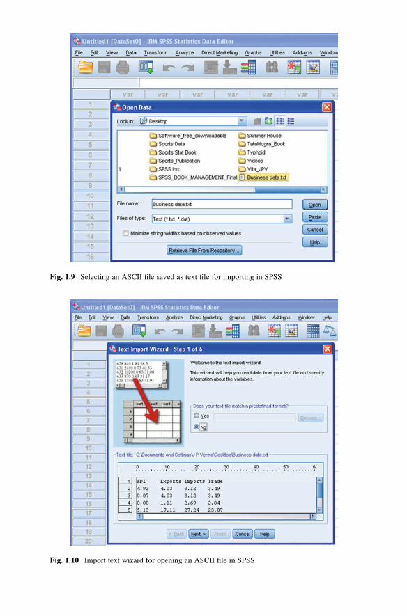
Fig. 1.10 Import text wizard for opening an ASCII file in SPSS
Fig. 1.9 Selecting an ASCII file saved as text file for importing in SPSS

Fig. 1.11 Defining option for delimiter and header row
Fig. 1.12 Defining option for beginning line of data and number of cases to be selected

variable name in the first line of the data file, line 1 is selected; otherwise, line
2 may be selected as the data starts from line 2 in the data file. Take the following
steps:
– Check the option “Each line represents a case.” Normally in your data file,
each line represents a case.
– Check the option “All of the cases.” Usually, you import all the cases from the
file. Other option may be tried if only few cases are imported from the file.
Click Next to get the screen as shown in Fig. 1.13.
5. In Fig. 1.13, delimiters of the data file (probably comma or space) are set:
– Check the delimiters as “Coma” as the data is separated by comma. Other
delimiters may be selected if used in the data file.
– Check the “Double quote” as text qualifier. Other options may be checked if
the variables are flanked other than double quote.
– On the basis of the options chosen by you, SPSS formats the file in the small
screen in the bottom. There you can check if everything is set correctly. Click
Next when everything is ok to get the screen as shown in Fig. 1.14.
Fig. 1.13 Defining option for delimiters and text qualifier
Importing Data in SPSS 21

6. In Fig. 1.14, you can define the specifications for the variables, but you may just
ignore it if you have already defined your variables or want to do it later. Click
Next to get the screen as shown in Fig. 1.15.
7. In Fig. 1.15, select all the default options and ensure that your actual data file has
been shown in the window or not. Once your data is shown in the window, click
Finish. This will import your file successfully in SPSS.
Importing Data File from Excel Format
The data prepared in Excel file can be imported in SPSS by simple command. While
importing Excel data file, one must ensure that it is not open. The sequence of
commands for importing Excel data file is as follows:
1. File�> Open�> Data�> requiredfile
– Choose “Excel” as the File Type if your ASCII file has the .xls extension.
Otherwise, choose the option “All files.”
– After selecting the file that you want to import, click Open as shown in
Fig. 1.16.
Fig. 1.14 Defining specifications for the variables
22 1 Data Management
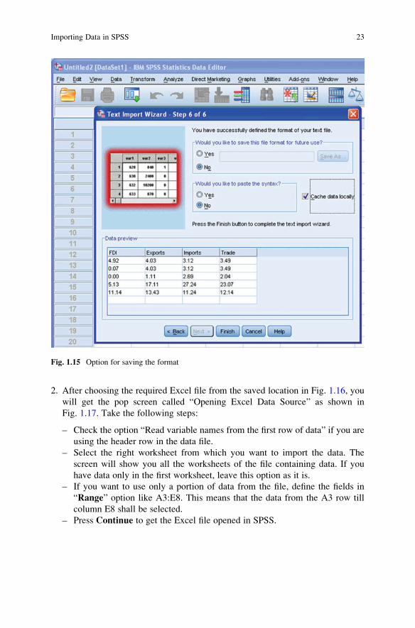
2. After choosing the required Excel file from the saved location in Fig. 1.16, you
will get the pop screen called “Opening Excel Data Source” as shown in
Fig. 1.17. Take the following steps:
– Check the option “Read variable names from the first row of data” if you are
using the header row in the data file.
– Select the right worksheet from which you want to import the data. The
screen will show you all the worksheets of the file containing data. If you
have data only in the first worksheet, leave this option as it is.
– If you want to use only a portion of data from the file, define the fields in
“Range” option like A3:E8. This means that the data from the A3 row till
column E8 shall be selected.
– Press Continue to get the Excel file opened in SPSS.
Fig. 1.15 Option for saving the format
Importing Data in SPSS 23

Fig. 1.16 Selecting an Excel file for importing in SPSS
Fig. 1.17 Option for defining the range of data in Excel sheet to be imported in SPSS
24 1 Data Management

Exercise
Short-Answer Questions
Note: Write the answer to each of the questions in not more than 200 words.
Q.1. What do you mean by inductive and inferential statistics? What is the differ-
ence between them? Explain by means of example.
Q.2. What do you mean by metric and nonmetric data? Discuss them by means of
example.
Q.3. Under what situation analytical studies should be conducted? Discuss a situa-
tion where it can be used.
Q.4. What do you mean by mutually exclusive and independent attributes? Give
two examples where the attributes are not mutually exclusive.
Q.5. What is an extraneous variable? How it affects the findings of an experiment?
Suggest remedies for eliminating its effects.
Q.6. While feeding the data in SPSS, what are the possible mistakes that a user
might commit?
Q.7. Explain in brief as to how an error can be identified in data feeding.
Multiple-Choice Questions
Note: For each of the question, there are four alternative answers. Tick mark the
one that you consider the closest to the correct answer.
1. Given the following statements,
I. Parametric tests do not assume anything about the form of the distribution.
II. Nonparametric tests are simple to use.
III. Parametric tests are the most powerful if their assumptions are satisfied.
IV. Nonparametric tests are based upon the assumption of normality.
choose the correct statements from the above-listed ones.
(a) (I) and (II)
(b) (I) and (III)
(c) (II) and (III)
(d) (III) and (IV)
2. If the respondents were required to rate themselves on emotional strength on a
9-point scale, what type of data would be generated?
(a) Ratio
(b) Interval
(c) Nominal
(d) Ordinal
Exercise 25

3. The variable measured on which of the following scales are termed as
categorical.
(a) Ratio and interval
(b) Interval and ordinal
(c) Interval and nominal
(d) Ordinal and nominal
4. In tossing an unbiased coin, one can get the following events:
E1: getting a head, E2: getting a tail. Choose the correct statement.
(a) E1 and E2 are independent.
(b) E1 and E2 are mutually exclusive.
(c) E1 and E2 are not equally likely.
(d) E1 and E2 are independent and mutually exclusive.
5. While creating a new data file in SPSS, which option should be used?
(a) Type in data
(b) Open an existing data source
(c) Open another type of file
(d) None
6. Identify valid name of the variable.
(a) SalesData
(b) Cust No
(c) Outlet “ Center”
(d) Sales-Data
7. While defining the types of the variable under the heading “Measure” in SPSS,
what are the valid options out of the following?
(i) Interval (ii) Scale
(iii) Nominal (iv) Ordinal
(a) (i),(ii), and (iii)
(b) (i),(ii), and (iv)
(c) (i),(iii), and (iv)
(d) (ii),(iii), and (iv)
8. For analyzing the data, the commands are selected while being in the
(a) Variable View
(b) Data View
(c) Data and Variable View
(d) Neither in Data nor in Variable View
26 1 Data Management

9. Runs scored in a cricket match is
(a) Interval data
(b) Ratio data
(c) Nominal data
(d) Ordinal data
10. In an experiment, effect of three types of incentives on satisfaction level has to
be seen on the subjects. Choose the correct statement.
(a) Incentive is a dependent variable, and satisfaction level is an independent
variable.
(b) Incentive is an independent variable, and satisfaction level is a dependent
variable.
(c) Incentive and satisfaction level are independent variables.
(d) Incentive and satisfaction level both are dependent variables.
Answers to Multiple-Choice Questions
Q.1 c Q.2 b
Q.3 d Q.4 b
Q.5 a Q.6 a
Q.7 d Q.8 b
Q.9 b Q.10 b
Exercise 27
Chapter 2
Descriptive Analysis
Learning Objectives
After completing this chapter, you should be able to do the following:
• Learn the importance of descriptive studies.
• Know the various statistics used in descriptive studies.
• Understand the situations in management research for undertaking a descriptive
study.
• Describe and interpret various descriptive statistics.
• Learn the procedure of computing descriptive statistics using SPSS.
• Know the procedure of developing the profile chart of a product or organization.
• Discuss the findings in the outputs generated by the SPSS in a descriptive study.
Introduction
Descriptive studies are carried out to understand the profile of any organization that
follows certain common practice. For example, one may like to know or be able to
describe the characteristics of an organization that implement flexible working
timing or that have a certain working culture. Descriptive studies may be
undertaken to describe the characteristics of a group of employees in an organiza-
tion. The purpose of descriptive studies is to prepare a profile or to describe
interesting phenomena from an individual or an organizational point of view.
Although descriptive studies can identify sales pattern over a period of time or in
different geographical locations but cannot ascertain the causal factors. These
studies are often very useful for developing further research hypotheses for testing.
Descriptive research may include case studies, cross-sectional studies, or longitu-
dinal investigations.
Different statistics are computed in descriptive studies to describe the nature of data.
These statistics computed from the sample provide summary of various measures.
Descriptive statistics are usually computed in all most every experimental research
J.P. Verma, Data Analysis in Management with SPSS Software,DOI 10.1007/978-81-322-0786-3_2, # Springer India 2013
29

study. The primary goal in a descriptive study is to describe the sample at any specific
point of time without trying to make inferences or causal statements. Normally, there
are three primary reasons to conduct such studies:
1. To understand an organization by knowing its system
2. To help in need assessment and planning resource allocation
3. To identify areas of further research
Descriptive studies help in identifying patterns and relationships that might
otherwise go unnoticed.
A descriptive study may be undertaken to ascertain and be able to describe the
characteristics of variables of interest, in a given situation. For instance, a study of
an organization in terms of percentage of employee in different age categories, their
job satisfaction level, motivation level, gender composition, and salary structure
can be considered as descriptive study. Quite frequently descriptive studies are
undertaken in organizations to understand the characteristics of a group or
employees such as age, educational level, job status, and length of service in
different departments.
Descriptive studies may also be undertaken to know the characteristics of all
those organizations that operate in the same sector. For example, one may try to
describe the production policy, sales criteria, or advertisement campaign in phar-
macy companies. Thus, the goal of descriptive study is to offer the researcher a
profile or to describe relevant aspects of the phenomena of interest in an organiza-
tion, industry, or a domain of population. In many cases, such information may be
vital before considering certain corrective steps.
In a typical profile study, we compute various descriptive statistics like mean,
standard deviation, coefficient of variation, range, skewness, and kurtosis. These
descriptive statistics explain different features of the data. For instance, mean
explains an average value of the measurement, whereas standard deviation
describes variation of the scores around their mean value; the coefficient of varia-
tion provides relative variability of scores; range gives the maximum variation;
skewness explains the symmetricity; and kurtosis describes the variation in the
data set.
In descriptive studies, one tries to obtain information regarding current status of
different phenomena. Purpose of such study is to describe “What exists?” with
respect to situational variables.
In descriptive research, the statement of problem needs to be defined first and
then identification of information is planned. Once the objectives of the study are
identified, method of data collection is planned to obtain an unbiased sample, and
therefore, it is important to define the population domain clearly. Further, an
optimum sample size should be selected for the study as it enhances the efficiency
in estimating population characteristics.
Once the data is collected, it should be compiled in a meaningful manner for
further processing and reporting. The nature of each variable can be studied by
looking to the values of different descriptive statistics. If purpose of the study is
30 2 Descriptive Analysis
analytical as well, then these data may further be analyzed for testing different
formulated hypotheses.
On the basis of descriptive statistics and graphical pictures of the parameters,
different kinds of generalizations and predictions can be made. While conducting
descriptive studies, one gets an insight to identify the future scope of the related
research studies.
Measures of Central Tendency
Researchers are often interested in defining a value that best describes some
characteristics of the population. Often, this characteristic is a measure of central
tendency. A measure of central tendency is a single score that attempts to describe a
set of data by identifying the central position within that set of data. The three most
common measures of central tendency are the mean, the median, and the mode.
Measures of central tendency are also known as central location. Perhaps, you are
more familiar with the mean (also known as average) as the measure of central
tendency, but there are others, such as the median and the mode, which are
appropriate in some specific situations.
The mean, median, and mode are all valid measures of central tendency, but,
under different conditions, some measures of central tendency become more appro-
priate than other. In the following sections, we will look at the various features of
mean, median, and mode and the conditions under which they are most appropriate
to be used.
Mean
The mean is the most widely used and popular measure of central tendency. It is
also termed as average. It gives an idea as to how an average score looks like.
For instance, one might be interested to know that on an average how much is the
sale of items per day on the basis of monthly sales figure. The mean is a good
measure of central tendency for symmetric distributions but may be misleading in
case of skewed distribution. The mean can be computed with both discrete and
continuous data. The mean is obtained by dividing the sum of all scores by the
number of scores in the data set.
If X1, X2, . . ., Xn are the n scores in the data set, then the sample mean, usually
denoted by �X (pronounced X bar), is
�X ¼ X1 þ X2 þ ::::Xn
n
Measures of Central Tendency 31
This formula is usually written by using the Greek capital letterP
, pronounced
“sigma,” which means “sum of. . .”:
�X ¼ 1
n
XX (2.1)
In statistics, sample mean and population mean are represented in different
manner, although the formulas for their computations are same. To show that we
are calculating the population mean and not the sample mean, we use the Greek
lower case letter “mu,” denoted as m:
m ¼ 1
n
XX
The mean is the model of your data set and explains that on an average, the data
set tends to concentrate toward it. You may notice that the mean is not often one of
the actual values that you have observed in your data set.
Computation of Mean with Grouped Data
If X1, X2, X3, . . ., Xn are n scores with f1, f2, f3, . . ., fn frequencies respectively in thedata set, then the mean is computed as
�X ¼P
fiXiPfi
¼P
fiXi
n(2.2)
wherePf iXi is the total of all the scores.
In case the data is arranged in class interval format, the X will be the midpoint of
the class interval. Let us see how to explain the data shown in the class interval form
in Table 2.1. The first class interval shows that the ten articles are in the price range
of Rs. 1–50 and that of six articles are in the range of Rs. 51–100 and so on. Here,
the exact price of each article is not known because they have been grouped
together. Thus, in case of grouped data, the scores lose its own identity. This
becomes problematic as it is difficult to add the scores because their magnitudes
are not known. In order to overcome this problem, an assumption is made while
computing mean and standard deviation from the grouped data. It is assumed that
the frequency is concentrated at the midpoint of the class interval. By assuming so,
the identity of each and every score can be regained; this helps us to compute the
sum of all the scores which is required for computing mean and standard deviation.
But by taking this assumption, it is quite likely that the scores may be either
underestimated or overestimated. For instance, in Table 2.1, if all the ten items
32 2 Descriptive Analysis
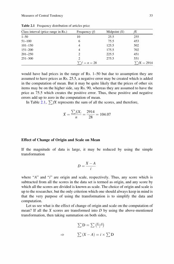
would have had prices in the range of Rs. 1–50 but due to assumption they are
assumed to have prices as Rs. 25.5, a negative error may be created which is added
in the computation of mean. But it may be quite likely that the prices of other six
items may be on the higher side, say Rs. 90, whereas they are assumed to have the
price as 75.5 which creates the positive error. Thus, these positive and negative
errors add up to zero in the computation of mean.
In Table 2.1,P
fX represents the sum of all the scores, and therefore,
�X ¼P
fiXi
n¼ 2914
28¼ 104:07
Effect of Change of Origin and Scale on Mean
If the magnitude of data is large, it may be reduced by using the simple
transformation
D ¼ X � A
i
where “A” and “i” are origin and scale, respectively. Thus, any score which is
subtracted from all the scores in the data set is termed as origin, and any score by
which all the scores are divided is known as scale. The choice of origin and scale is
up to the researcher, but the only criterion which one should always keep in mind is
that the very purpose of using the transformation is to simplify the data and
computation.
Let us see what is the effect of change of origin and scale on the computation of
mean? If all the X scores are transformed into D by using the above-mentioned
transformation, then taking summation on both sides,
PD ¼P X�A
i
� �) P
X � Að Þ ¼ i�PD
Table 2.1 Frequency distribution of articles price
Class interval (price range in Rs.) Frequency (f) Midpoint (X) fX
1–50 10 25.5 255
51–100 6 75.5 453
101–150 4 125.5 502
151–200 4 175.5 702
201–250 2 225.5 451
251–300 2 275.5 551Pf ¼ n ¼ 28
PfX ¼ 2914
Measures of Central Tendency 33

Dividing both side by n,
PX � Að Þn
¼ i�PD
n
) 1
n
XX � nA
n¼ i� 1
n
XD
) �X ¼ Aþ i� �D
Thus, we have seen that if all the scores X are transformed intoD by changing the
origin and scales as A and i, respectively, then the original mean can be obtained
by multiplying the new mean �D by the scale i and adding the origin value into it.
Thus, it may be concluded that the mean is not independent of change of origin and
scale.
Computation of Mean with Deviation Method
In case of grouped data, the mean can be computed by transforming the scores so
obtained by taking the midpoint of the class intervals. Consider the data shown in
Table 2.1 once again. After computing the midpoint of the class intervals, let us
transform the scores by changing the origin and scale as 175.5 and 50, respectively.
Usually, origin (A) is taken as the midpoint of the middlemost class interval, and the
scale (i) is taken as the width of the class interval. The origin A is also known as
assumed mean (Table 2.2).
Here, width of the class interval ¼ i ¼ 50 and assumed mean A ¼ 175.5
Since we know that
X ¼ Aþ i� D ¼ Aþ i� 1
n
XfD
) �X ¼ 175:5þ 50� 1
28� ð�40Þ
¼ 175:5� 71:43 ¼ 104:07
Table 2.2 Showing computation for mean
Class interval
(price range in Rs.) Frequency (f) Midpoint (X) D ¼ X�175:550
fD
1–50 10 25.5 �3 �30
51–100 6 75.5 �2 �12
101–150 4 125.5 �1 �4
151–200 4 175.5 0 0
201–250 2 225.5 1 2
251–300 2 275.5 2 4Pf ¼ n ¼ 28
PfD ¼ �40
34 2 Descriptive Analysis

In computing the mean, the factor i� 1 n=ð ÞP fD can be considered as the
correction factor. If the assumed mean is taken higher than the actual mean, the
correction factor shall be negative, and, if it is taken as lower than the actual mean,
the correction factor will become positive. One may take assume mean as the
midpoint of the even lowest or highest class interval. But in that case, the magnitude
of the correction factor shall be higher and the very purpose of simplifying the
computation process shall be defeated. Thus, the correct strategy is to take the
midpoint of the middlemost class interval as the assumed mean. However, in case
the number of class intervals is even, midpoint of any of the two middle class
intervals may be taken as the assumed mean.
Properties of Mean
1. The mean is the most reliable measure of central tendency as it is computed by
using all the data in the data set.
2. Mean is more stable than any other measures of central tendency because its
standard error is least in comparison to median and mode. It simply means that if
you compute mean of different samples that are drawn from the same popula-
tion, then the fluctuation among these means shall be least in comparison to that
of other measures of central tendencies like median and mode.
3. If �X1 and �X2 are the means of the two groups computed from the two sets of
values n1 and n2, then the combined mean �Xis given by the following formula:
�X ¼ n1 �X1 þ n2 �X2
n1 þ n2
4. The sum of the deviation of a set of values from their arithmetic mean is always
0. In other words,
XX � �Xð Þ ¼ 0
To prove this, expand left-hand side of this expression
XX � �Xð Þ ¼
XX �
X�X
¼ N �X � N �X ¼ 0
5. The mean is highly affected by the outliers.
6. In the absence of even one observation, it is impossible to compute the mean
correctly.
7. In case of open-ended class interval, the mean cannot be computed.
Measures of Central Tendency 35

Median
Median is the middlemost score in the data set arranged in order of magnitude. It is
a positional average and is not affected by the extreme scores. If X1, X2, . . ., Xn are
the n scores in a data set arranged in the ascending or descending order, then its
median is obtained by
Md ¼ N þ 1
2
� �th
score (2.4)
One should note that nþ 1ð Þ=2 is not the median, but the score lying in that
position is the median. Consider the weight of the following ten subjects: 56, 45, 53,
41, 48, 53, 52, 65, 38, 42.
After arranging the scores
S.N.: 1 2 3 4 5 6 7 8 9 10
Weight: 38 41 42 45 48 52 53 53 56 65
Here, n ¼ 10.
Thus, Md ¼ 10þ12
� �th ¼ 5:5thscore ¼ 48þ52ð Þ2
¼ 50
In case of odd number of scores you will get a single score lying in the middle,
but in case of even number of scores, the middlemost score is obtained by taking the
average of the two middle scores as in that case there are two middle scores.
Median is used in case the effect of extreme scores needs to be avoided. For
example, consider the marks of the students in a college as shown below:
Student: 1 2 3 4 5 6 7 8 9 10
Marks: 35 40 30 32 35 39 33 32 91 93
The mean score for these ten students is 46. However, the raw data suggests that
this mean value might not be the best way to accurately reflect the typical perfor-
mance of a student, as most students have marks in between 30 and 40. Here, the
mean is being skewed by the two large scores. Therefore, in this situation, median
gives better estimate of average instead of mean. Thus, in a situation where the
effect of extreme scores needs to be avoided, median should be preferred over
mean. In case the data is normally distributed, the values of mean, median, and
mode are same. Moreover, they all represent the most typical value in the data set.
However, as the data becomes skewed, the mean loses its ability to provide the best
central location as the mean is being dragged in the direction of skew. In that case,
the median best retains this position and is not influenced much by the skewed
values. As a rule of thumb if the data is non-normal, then it is customary to use the
median instead of the mean.
36 2 Descriptive Analysis

Computation of Median for Grouped Data
While computing the median for grouped data, it is assumed that the frequencies are
equally distributed in the class interval. This assumption is also used in computing
the quartile deviation because median and quartile deviation both are nonparamet-
ric statistics and depend upon positional score. In case of grouped data, the median
is computed by the following formula:
Md ¼ jj þn2� F
f m� i (2.5)
where
|| : lower limit of the median class
n : total of all the frequencies
F : cumulative frequency of the class just lower than the median class
fm : frequency of the median class
i : width of the class interval
The computation of the median shall be shown by means of an example.
Consider the marks in mathematics obtained by the students as shown in Table 2.3.
In computing median, first of all we need to find the median class. Median class
is the one in which the median is supposed to lie. To obtain the median class, we
compute n/2 and then we look for this value in the column of cumulative frequency.
The class interval for which the cumulative frequency includes the value n/2 is
taken as median class.
Here, n ¼ 70
and therefore, n2¼ 70
2¼ 35
Now, we look for 35 in the column of cumulative frequency. You can see that
the class interval 31–35 has a cumulative frequency 48 which includes the value
n/2 ¼ 35. Thus, 31–35 is the median class. After deciding the median class, the
median can be computed by using the formula (2.5).
Here, || ¼ Lower limit of the median class ¼ 30.5
fm ¼ Frequency of the median class ¼ 20
F ¼ Cumulative frequency of the class just lower than the median class ¼ 28
i ¼ Width of the class interval ¼ 5
Substituting these values in the formula (2.5),
Md ¼ jj þn2� F
f m� i
¼ 30:5þ 35� 28
20� 5 ¼ 30:50þ 1:75 ¼ 32:25
In computing the lower limit of the median class, 0.5 has been subtracted from
the lower limit because the class interval is discrete. Any value which is equal or
Measures of Central Tendency 37
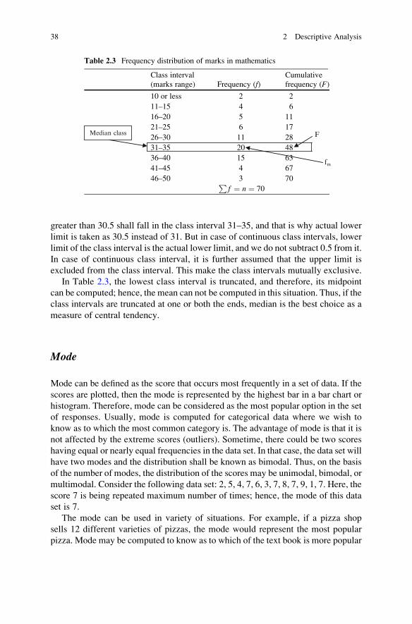
greater than 30.5 shall fall in the class interval 31–35, and that is why actual lower
limit is taken as 30.5 instead of 31. But in case of continuous class intervals, lower
limit of the class interval is the actual lower limit, and we do not subtract 0.5 from it.
In case of continuous class interval, it is further assumed that the upper limit is
excluded from the class interval. This make the class intervals mutually exclusive.
In Table 2.3, the lowest class interval is truncated, and therefore, its midpoint
can be computed; hence, the mean can not be computed in this situation. Thus, if the
class intervals are truncated at one or both the ends, median is the best choice as a
measure of central tendency.
Mode
Mode can be defined as the score that occurs most frequently in a set of data. If the
scores are plotted, then the mode is represented by the highest bar in a bar chart or
histogram. Therefore, mode can be considered as the most popular option in the set
of responses. Usually, mode is computed for categorical data where we wish to
know as to which the most common category is. The advantage of mode is that it is
not affected by the extreme scores (outliers). Sometime, there could be two scores
having equal or nearly equal frequencies in the data set. In that case, the data set will
have two modes and the distribution shall be known as bimodal. Thus, on the basis
of the number of modes, the distribution of the scores may be unimodal, bimodal, or
multimodal. Consider the following data set: 2, 5, 4, 7, 6, 3, 7, 8, 7, 9, 1, 7. Here, the
score 7 is being repeated maximum number of times; hence, the mode of this data
set is 7.
The mode can be used in variety of situations. For example, if a pizza shop
sells 12 different varieties of pizzas, the mode would represent the most popular
pizza. Mode may be computed to know as to which of the text book is more popular
Table 2.3 Frequency distribution of marks in mathematics
Class interval
(marks range) Frequency (f)Cumulative
frequency (F)
10 or less 2 2
11–15 4 6
16–20 5 11
21–25 6 17
26–30 11 28
31–35 20 48
36–40 15 63
41–45 4 67
46–50 3 70Pf ¼ n ¼ 70
F
fm
Median class
38 2 Descriptive Analysis

than others, and accordingly, the publisher would print more copy of that book
instead of printing equal number of all books.
Similarly, it is important for the manufacturer to produce more of the most
popular shoes because manufacturing different shoes in equal numbers would cause
a shortage of some shoes and an oversupply of others. Other applications of the
mode may be to find the most popular brand of soft drink or biscuits to take the
manufacturing decision accordingly.
Drawbacks of Mode
1. Computing mode becomes problematic if the data set consists of continuous
data, as we are more likely not to have any one value that is more frequent than
the other. For example, consider measuring 40 persons’ height (to the nearest
1 cm). It will be very unlikely that any two or more people will have the same
height. This is why the mode is very rarely used with continuous data.
2. Mode need not necessarily be unique. There may be more than one mode present
in the data set. In that case, it is difficult to interpret and compare the mode.
3. If no value in the data set is repeated, then every score is a mode which is useless.
Computation of Mode for Grouped Data
In computing the mode with grouped data first of all one needs to identify the modal
class. The class interval, for which the frequency is maximum, is taken as modal
class. The frequency of the modal class is denoted by f0, and that of frequencies
before and after the modal class are represented by f1 and f2, respectively. Oncethese frequencies are identified, they can be used to compute the value of the mode.
The formula for computing mode with the grouped data is given by
M0 ¼ jj þ fm � f1
2fm � f1 � f2� i (2.6)
where
|| : lower limit of the modal class
fm : frequency of the modal class
f1 : frequency of the class just lower than the modal class
f2 : frequency of the class just higher than the modal class
i : width of the class interval
Table 2.4 shows the distribution of age of bank employees. Let us compute the
value of mode in order to find as to what is the most frequent age of employees in
the bank.
Since the maximum frequency is 50 for the class interval 26–30, hence this will
be the modal class here.
Measures of Central Tendency 39

Now, || ¼ lower limit of the modal class ¼ 25.5
fm : frequency of the modal class ¼ 50
f1 : frequency of the class just lower than the modal class ¼ 25
f2 : frequency of the class just higher than the modal class ¼ 10
i : width of the class interval ¼ 5
After substituting these values in the formula (2.6), we get
M0 ¼ jj þ fm � f1
2fm � f1 � f2� i
¼ 25:5þ 50� 25
2� 50� 25� 10� 5
¼ 25:5þ 1:92 ¼ 27:42
Thus, one may conclude that mostly employees in the bank are of around
27 years of age.
Summary of When to Use the Mean, Median, and Mode
Following summary table shows the suitability of different measures of central
tendency for different types of data.
Nature of variable Suitable measure of central tendency
Nominal data (categorical) Mode
Ordinal data Median
Interval/ratio (symmetrical or nearly symmetrical) Mean
Interval/ratio (skewed) Median
Table 2.4 Frequency distribution of age
Class interval C.I. Frequency (f)
21–25 25
26–30 50
31–35 10
36–40 5
41–45 4
46–50 2
40 2 Descriptive Analysis

Measures of Variability
Variability refers to the extent of scores that vary from each other. The data set is
said to have high variability when it contains values which are considerably higher
and lower than the mean value. The terms variability, dispersion, and spread are all
synonyms and refer as to how much the distribution is spread out. Measure of
central tendency refers to the central location in the data set, but the central location
itself is not sufficient to define the characteristics of the data set. It may happen that
the two data sets are similar in their central location but might differ in their
variability. Thus, measure of central tendency and measure of variability both are
required to describe the nature of the data correctly. There are four measures of
variability that are frequently used, the range: interquartile range, variance, and
standard deviation. In the following paragraphs, we will look at each of these four
measures of variability in more detail.
The Range
The range is the crudest measure of variability and is obtained by subtracting the
lowest score from the highest score in the data set. It is rarely used because it is
based on only two extreme scores. The range is simple to compute and is useful
when it is required to evaluate the whole of a data set. The range is useful in
showing the maximum spread within a data set. It can be used to compare the spread
between similar data sets.
Using range becomes problematic if one of the extreme score is exceptionally
high or low (referred to as outlier). In that case, the range so computed may not
represent the true variability within the data set. Consider a situation where scores
obtained by the students on a test were recorded and the minimum and maximum
scores were 25 and 72, respectively. If a particular student did not appear in the
exam due to some reason and his score was posted as zero, then the range becomes
72(72–0) instead of 47(72–25). Thus, in the presence of an outlier, the range
provides the wrong picture about the variability within the data set. To overcome
the problem of outlier in a data set, the interquartile range is often calculated instead
of the range.
The Interquartile Range
The interquartile range is a measure that indicates the maximum variability of the
central 50% of values within the data set. The interquartile range can further be
divided into quarters by identifying the upper and lower quartiles. The lower
quartile (Q1) is equivalent to the 25th percentile in the data set which is arranged
in order of magnitude, whereas the upper quartile (Q3) is equivalent to the 75th
Measures of Variability 41

percentile. Thus, Q1 is a point below which 25% scores lie, and Q3 refers to a score
below which 75% scores lie. Since the median is a score below which 50% scores
lie, hence, the upper quartile lies halfway between the median and the highest value
in the data set, whereas the lower quartile lies halfway between the median and the
lowest value in the data set. The interquartile range is computed by subtracting the
lower quartile from the upper quartile and is given by
Q ¼ Q3 � Q1 (2.7)
The interquartile range provides a better picture of the overall data set by
ignoring the outliers. Just like range, interquartile range also depends upon the
two values. Statistically, the standard deviation is more powerful measure of
variability as it is computed with all the values in the data set.
The Standard Deviation
The standard deviation is the most widely used measure of variability, the value of
which depends upon how closely the scores cluster around the mean value. It can be
computed only for interval or ratio data. The standard deviation is the square root of
the average squared deviation of the scores from its mean value and is represented
by s(termed as sigma):
s ¼ffiffiffiffiffiffiffiffiffiffiffiffiffiffiffiffiffiffiffiffiffiffiffiffiffiffiffiffiffiffi1
N
XX � mð Þ2
r
After simplification,
s ¼ffiffiffiffiffiffiffiffiffiffiffiffiffiffiffiffiffiffiffiffiffiffiffiffiffiffiffiffiffiffiffiffiffiffiffiffiffiffiffiffiffiffi1
N
XX2 �
PX
N
� �2s
(2.8)
where m is the population mean. The terms is used for population standard deviation,whereas S is used for sample standard deviation. The population standard deviation scan be estimated from the sample data by the following formula:
S ¼ffiffiffiffiffiffiffiffiffiffiffiffiffiffiffiffiffiffiffiffiffiffiffiffiffiffiffiffiffiffiffiffiffiffiffiffiffiffi1
n� 1
XX � �Xð Þ2
r
After simplifying,
S ¼ffiffiffiffiffiffiffiffiffiffiffiffiffiffiffiffiffiffiffiffiffiffiffiffiffiffiffiffiffiffiffiffiffiffiffiffiffiffiffiffiffiffiffiffiffiffiffiffi1
n� 1
XX2 �
PXð Þ2
nðn� 1Þ
s(2.9)
42 2 Descriptive Analysis
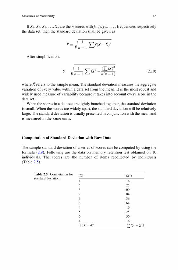
If X1, X2, X3, . . ., Xn are the n scores with f1, f2, f3,. . ., fn frequencies respectivelythe data set, then the standard deviation shall be given as
S ¼ffiffiffiffiffiffiffiffiffiffiffiffiffiffiffiffiffiffiffiffiffiffiffiffiffiffiffiffiffiffiffiffiffiffiffiffiffiffiffiffi1
n� 1
Xf X � �Xð Þ2
r
After simplification,
S ¼ffiffiffiffiffiffiffiffiffiffiffiffiffiffiffiffiffiffiffiffiffiffiffiffiffiffiffiffiffiffiffiffiffiffiffiffiffiffiffiffiffiffiffiffiffiffiffiffiffi1
n� 1
XfX2 �
PfXð Þ2
nðn� 1Þ
s(2.10)
where �X refers to the sample mean. The standard deviation measures the aggregate
variation of every value within a data set from the mean. It is the most robust and
widely used measure of variability because it takes into account every score in the
data set.
When the scores in a data set are tightly bunched together, the standard deviation
is small. When the scores are widely apart, the standard deviation will be relatively
large. The standard deviation is usually presented in conjunction with the mean and
is measured in the same units.
Computation of Standard Deviation with Raw Data
The sample standard deviation of a series of scores can be computed by using the
formula (2.9). Following are the data on memory retention test obtained on 10
individuals. The scores are the number of items recollected by individuals
(Table 2.5).
Table 2.5 Computation for
standard deviation(X) (X2)
4 16
5 25
3 09
2 04
6 36
8 64
4 16
5 25
6 36
4 16PX ¼ 47
PX2 ¼ 247
Measures of Variability 43
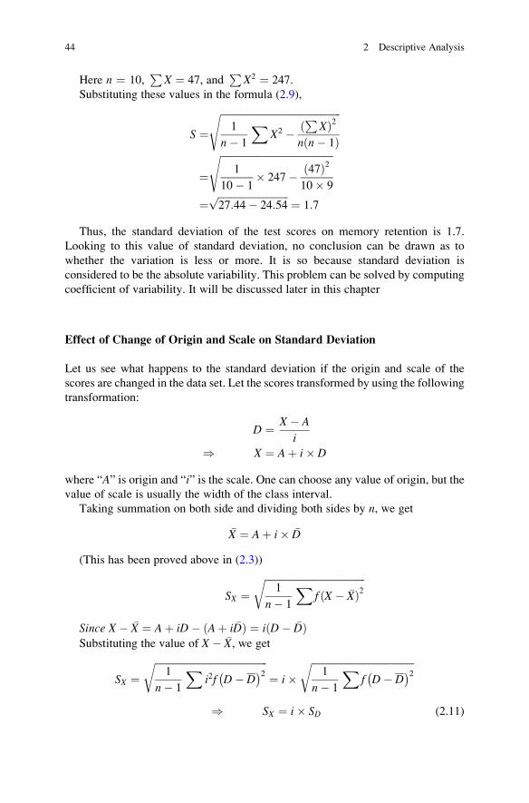
Here n ¼ 10,P
X ¼ 47, andP
X2 ¼ 247.
Substituting these values in the formula (2.9),
S ¼ffiffiffiffiffiffiffiffiffiffiffiffiffiffiffiffiffiffiffiffiffiffiffiffiffiffiffiffiffiffiffiffiffiffiffiffiffiffiffiffiffiffiffiffiffiffiffiffi1
n� 1
XX2 �
PXð Þ2
nðn� 1Þ
s
¼ffiffiffiffiffiffiffiffiffiffiffiffiffiffiffiffiffiffiffiffiffiffiffiffiffiffiffiffiffiffiffiffiffiffiffiffiffiffiffiffiffiffiffiffiffi
1
10� 1� 247� 47ð Þ2
10� 9
s
¼ffiffiffiffiffiffiffiffiffiffiffiffiffiffiffiffiffiffiffiffiffiffiffiffiffiffiffiffi27:44� 24:54
p¼ 1:7
Thus, the standard deviation of the test scores on memory retention is 1.7.
Looking to this value of standard deviation, no conclusion can be drawn as to
whether the variation is less or more. It is so because standard deviation is
considered to be the absolute variability. This problem can be solved by computing
coefficient of variability. It will be discussed later in this chapter
Effect of Change of Origin and Scale on Standard Deviation
Let us see what happens to the standard deviation if the origin and scale of the
scores are changed in the data set. Let the scores transformed by using the following
transformation:
D ¼ X � A
i
) X ¼ Aþ i� D
where “A” is origin and “i” is the scale. One can choose any value of origin, but thevalue of scale is usually the width of the class interval.
Taking summation on both side and dividing both sides by n, we get
�X ¼ Aþ i� �D
(This has been proved above in (2.3))
SX ¼ffiffiffiffiffiffiffiffiffiffiffiffiffiffiffiffiffiffiffiffiffiffiffiffiffiffiffiffiffiffiffiffiffiffiffiffiffiffiffiffi1
n� 1
Xf X � �Xð Þ2
r
Since X � �X ¼ Aþ iD� Aþ i �Dð Þ ¼ i D� �Dð ÞSubstituting the value of X � �X, we get
SX ¼ffiffiffiffiffiffiffiffiffiffiffiffiffiffiffiffiffiffiffiffiffiffiffiffiffiffiffiffiffiffiffiffiffiffiffiffiffiffiffiffiffiffiffiffiffi1
n� 1
Xi2f D� D� �2r
¼ i�ffiffiffiffiffiffiffiffiffiffiffiffiffiffiffiffiffiffiffiffiffiffiffiffiffiffiffiffiffiffiffiffiffiffiffiffiffiffiffiffiffi1
n� 1
Xf D� D� �2r
) SX ¼ i� SD (2.11)
44 2 Descriptive Analysis
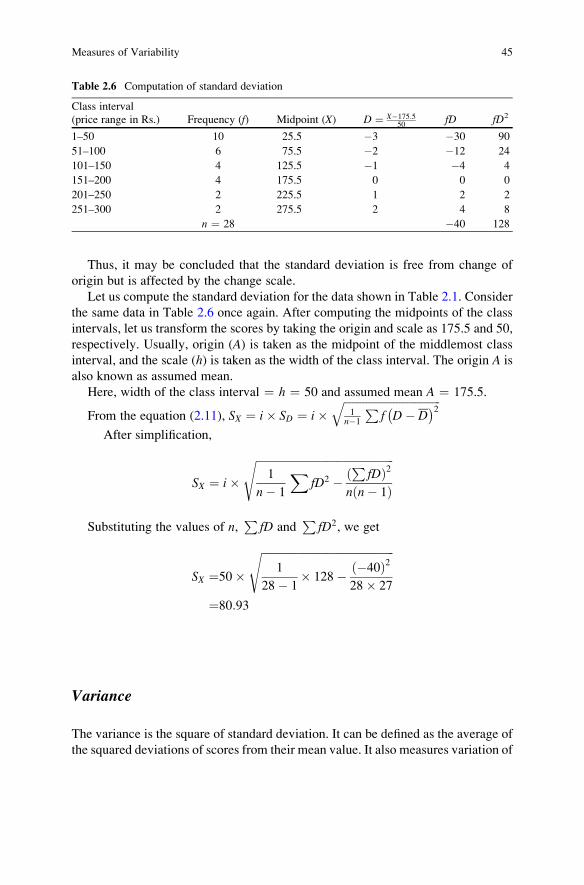
Thus, it may be concluded that the standard deviation is free from change of
origin but is affected by the change scale.
Let us compute the standard deviation for the data shown in Table 2.1. Consider
the same data in Table 2.6 once again. After computing the midpoints of the class
intervals, let us transform the scores by taking the origin and scale as 175.5 and 50,
respectively. Usually, origin (A) is taken as the midpoint of the middlemost class
interval, and the scale (h) is taken as the width of the class interval. The origin A is
also known as assumed mean.
Here, width of the class interval ¼ h ¼ 50 and assumed mean A ¼ 175.5.
From the equation (2.11), SX ¼ i� SD ¼ i�ffiffiffiffiffiffiffiffiffiffiffiffiffiffiffiffiffiffiffiffiffiffiffiffiffiffiffiffiffiffiffiffiffiffiffi1
n�1
Pf D� D� �2q
After simplification,
SX ¼ i�ffiffiffiffiffiffiffiffiffiffiffiffiffiffiffiffiffiffiffiffiffiffiffiffiffiffiffiffiffiffiffiffiffiffiffiffiffiffiffiffiffiffiffiffiffiffiffiffiffiffi1
n� 1
XfD2 �
PfDð Þ2
nðn� 1Þ
s
Substituting the values of n,P
fD andP
fD2, we get
SX ¼50�ffiffiffiffiffiffiffiffiffiffiffiffiffiffiffiffiffiffiffiffiffiffiffiffiffiffiffiffiffiffiffiffiffiffiffiffiffiffiffiffiffiffiffiffiffiffiffiffi
1
28� 1� 128� �40ð Þ2
28� 27
s
¼80:93
Variance
The variance is the square of standard deviation. It can be defined as the average of
the squared deviations of scores from their mean value. It also measures variation of
Table 2.6 Computation of standard deviation
Class interval
(price range in Rs.) Frequency (f) Midpoint (X) D ¼ X�175:550
fD fD2
1–50 10 25.5 �3 �30 90
51–100 6 75.5 �2 �12 24
101–150 4 125.5 �1 �4 4
151–200 4 175.5 0 0 0
201–250 2 225.5 1 2 2
251–300 2 275.5 2 4 8
n ¼ 28 �40 128
Measures of Variability 45

the scores in the distribution. It shows the magnitude of variation among the scores
around its mean value. In other words, it measures the consistency of data. Higher
variance indicates more heterogeneity, whereas lower variance represents more
homogeneity in the data.
Like standard deviation, it also measures the variability of scores that are
measured in interval or ratio scale. The variance is usually represented by s2andis computed as
s2 ¼ 1
N
XX � mð Þ2 (2.12)
The variance can be estimated from the sample by using the following formula:
s2 ¼ 1
n� 1
XX � �Xð Þ2
¼ 1
n� 1
XX2 �
PXð Þ2
nðn� 1Þ
Remark Population mean and population standard deviation are represented by mand s, respectively, whereas sample mean and sample standard deviation are
represented by �Xand S, respectively.
The Index of Qualitative Variation
Measures of variability like range, standard deviation, or variance are computed for
interval or ratio data. What if the data is in nominal form? In social research, one
may encounter many situations where it is required to measure the variability of the
data based on nominal scale. For example, one may like to find the variability of
ethnic population in a city, variation in the responses on different monuments,
variability in the liking of different sports in an institution, etc. In all these
situations, an index of qualitative variation (IQV) may be computed by the follow-
ing formula to find the magnitude of variability:
IQV ¼ K 1002 �PP2� �1002ðK � 1Þ (2.13)
where
K ¼ The number of categories
SP2 ¼ Sum of squared percentages of frequencies in all the groups
46 2 Descriptive Analysis
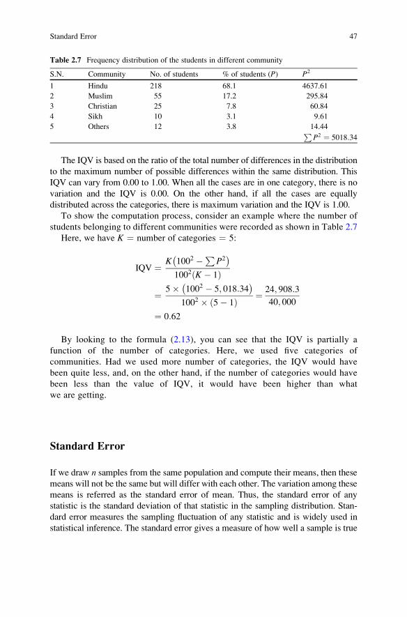
The IQV is based on the ratio of the total number of differences in the distribution
to the maximum number of possible differences within the same distribution. This
IQV can vary from 0.00 to 1.00. When all the cases are in one category, there is no
variation and the IQV is 0.00. On the other hand, if all the cases are equally
distributed across the categories, there is maximum variation and the IQV is 1.00.
To show the computation process, consider an example where the number of
students belonging to different communities were recorded as shown in Table 2.7
Here, we have K ¼ number of categories ¼ 5:
IQV ¼ K 1002 �PP2� �1002ðK � 1Þ
¼ 5� 1002 � 5; 018:34� �1002 � 5� 1ð Þ ¼ 24; 908:3
40; 000
¼ 0:62
By looking to the formula (2.13), you can see that the IQV is partially a
function of the number of categories. Here, we used five categories of
communities. Had we used more number of categories, the IQV would have
been quite less, and, on the other hand, if the number of categories would have
been less than the value of IQV, it would have been higher than what
we are getting.
Standard Error
If we draw n samples from the same population and compute their means, then these
means will not be the same but will differ with each other. The variation among these
means is referred as the standard error of mean. Thus, the standard error of any
statistic is the standard deviation of that statistic in the sampling distribution. Stan-
dard error measures the sampling fluctuation of any statistic and is widely used in
statistical inference. The standard error gives a measure of how well a sample is true
Table 2.7 Frequency distribution of the students in different community
S.N. Community No. of students % of students (P) P2
1 Hindu 218 68.1 4637.61
2 Muslim 55 17.2 295.84
3 Christian 25 7.8 60.84
4 Sikh 10 3.1 9.61
5 Others 12 3.8 14.44PP2 ¼ 5018:34
Standard Error 47

representative of the population. When the sample is truly representing the popula-
tion, the standard error will be small.
Constructing confidence intervals and testing of significance are based on standard
errors. The standard error of mean can be used to compare the observed mean to a
hypothesized value. The two values may be different at 5% level if the ratio of the
difference to the standard error is less than �2 or greater than +2.
The standard error of any statistics is affected by the sample size. In general, the
standard error decreases with the increase in sample size. It is denoted by s with a
subscript of a statistic for which it is computed.
Let �X1, �X2, �X3, . . ., �Xn are the means of n samples drawn from the same population.
Then the standard deviation of these n mean scores is said to be standard error of
mean. The standard error of sample mean can be estimated by even one sample. If
any sample consists of n scores with population standard deviation s, then the
standard error of the mean is given by
s �X ¼ sffiffiffin
p (2.14)
Whereas the standard error of the standard deviation is given by
ss ¼ sffiffiffiffiffi2n
p (2.15)
Like standard error of the mean, the standard error of the standard deviation also
measures the fluctuation of standard deviations among the samples.
Remark If population standard deviation s is unknown, it may be estimated by the
sample standard deviation S.
Coefficient of Variation (CV)
Coefficient of variation is an index which measures the extent of variability in the
data set in relation to its mean value. It is free from unit and compensates with the
value of mean in the data set. Coefficient of variation is also known as relative
variability and is denoted by CV
CV ¼ S�X� 100 (2.16)
where S and �X represent sample standard deviation and sample mean respectively.
Since coefficient of variation measures the relative variability and computes the
variability in percentage, it can be used to know whether a particular parameter is
more variable or less variable. Coefficient of variation can be used for comparing
the variability of two groups in a situation when their mean values are not equal.
48 2 Descriptive Analysis

It may also be used to compare the variability of two groups of data having different
units.
On the other hand, standard deviation is a measure of absolute variability, and
therefore, it cannot be used to assess the variability of any data set without knowing
its mean value. Further, standard deviation cannot be used to compare the
variability of two sets of scores if their mean value differs.
Consider the following statistics obtained on the number of customers visiting
the retail outlets of a company in two different locations in a month. Let us see what
conclusions can be drawn with this information.
Location A B
Mean 40 20
SD 8 6
CV 20% 30%
The standard deviation of the number of customers in location A is larger in
comparison to location B, whereas coefficient of variation is larger in location B in
comparison to location A. Thus, it may be inferred that the variation among the
number of customers visiting the outlet in location B is higher than that of location A.
Moments
A moment is a quantitative value that tells us the shape of a set of points. The
moment can be central or noncentral. Central moment is represented by mr, whereasnoncentral moment is denoted by m
0r . If the deviation of scores is taken around mean,
then the moment becomes central, and if it is taken around zero or any other arbitrary
value, it is known as noncentral moment. The rth central moment is given by
mr ¼1
n
XX � �Xð Þr (2.17)
Different moments convey different meanings. For instance, second central
moment m2 is always equal to variance of a distribution. Similarly second, third,
and fourth moments are used to compute skewness and kurtosis of the data set. On
the other hand, rth noncentral moment around the origin zero is denoted by
m0r ¼
1
n
XXr (2.18)
Moments 49

The first noncentral moment m01 about zero always represents mean of the
distribution. These noncentral moments are used to compute central moments by
means of a recurrence relation.
Skewness
Skewness gives an idea about the symmetricity of the data. In symmetrical distri-
bution if the curve is divided in the middle, the two parts become the mirror image
of each other. If the curve is not symmetrical, it is said to be skewed. The skewness
of the distribution is represented by b1and is given by
b1 ¼m23m32
(2.19)
where m2 and m3 are the second and third central moments. For a symmetric
distribution, b1 is 0. A distribution is positively skewed if b1 is positive and
negatively skewed if it is negative. In a positively skewed distribution, the tail is
heavy toward the right side of the curve, whereas in a negatively skewed curve, the
tail is heavy toward the left side of the curve. Further, in positively skewed curve,
median is greater than mode, whereas in negatively skewed curve, the median is
less than mode. Graphically both these curves can be shown by Fig. 2.1a, b:
The standard error of the skewness is given by
SEðSkewnessÞ ¼ SE b1ð Þ ¼ffiffiffiffiffiffiffiffiffiffiffiffiffiffiffiffiffiffiffiffiffiffiffiffiffiffiffiffiffiffiffiffiffiffiffiffiffiffiffiffiffiffiffi
6nðn� 1Þðn� 2Þðnþ 1Þðnþ 3Þ
s(2.20)
where n is the sample size. Some authors useffiffiffiffiffiffiffiffi6=n
pfor computing standard error of
the skewness, but it is a poor approximation for the small sample.
The standard error of skewness can be used to test its significance. In testing the
significance of skewness, the following Z statistic is used which follows a normal
distribution.
Z ¼ffiffiffiffiffiffiffiffiffiffiffiffiffiffiffiffiffinðn� 1Þpn� 2
� b1SE b1ð Þ (2.21)
The critical value of Z is approximately 2 (for a two-tailed test with roughly at 5%
level). Thus, if calculated value of Z < �2, we may interpret that the population is
50 2 Descriptive Analysis

very likely to be skewed negatively. On the other hand, if calculated Z > +2, it may
be concluded that the population is positively skewed.
However, in general, skewness values more than twice its standard error
indicates a departure from symmetry. This gives a criterion to test whether skew-
ness (positive or negative) in the distribution is significant or not. Thus, if the data is
positively skewed, it simply means that majority of the scores are less than its mean
value, and in case of negative skewness, most of the scores are more than its mean
value.
Kurtosis
Kurtosis is a statistical measure used for describing the distribution of observed data
around the mean. It measures the extent to which the observations cluster around
the mean value. It is measured by (Gamma) and is computed as
g ¼ b2 � 3 (2.22)
where b2 ¼ m4m22
, m2 and m4 represent the second and fourth central moments
respectively.
For a normal distribution, the value of kurtosis ðgÞ is zero. Positive value of
kurtosis in a distribution indicates that the observations cluster more around its
mean value and have longer tails in comparison to that of normal distribution,
whereas a distribution with negative kurtosis indicates that the observations cluster
less around its mean and have shorter tails.
Depending upon the value of kurtosis, the distribution of scores can be classified
into any one of the three categories: leptokurtic, mesokurtic, and platykurtic.
If for any variable the kurtosis is positive, the curve is known as leptokurtic and
it represents a low level of data fluctuation, as the observations cluster around the
mean. On the other hand, if the kurtosis is negative, the curve is known as
platykurtic and it means that the data has a larger degree of variance. In other
words, if the value of kurtosis is significant and positive, it signifies less variability
in the data set or we may say that the data is more homogenous. On the other hand,
significant negative kurtosis indicates that there is more variability in the data set or
we may conclude that the data is more heterogeneous. Further, if the kurtosis is 0,
a b
Mod
eM
edia
nM
ean
Mod
eM
edia
nM
ean
Fig. 2.1 (a and b) Showing positively and negatively skewed curve
Kurtosis 51
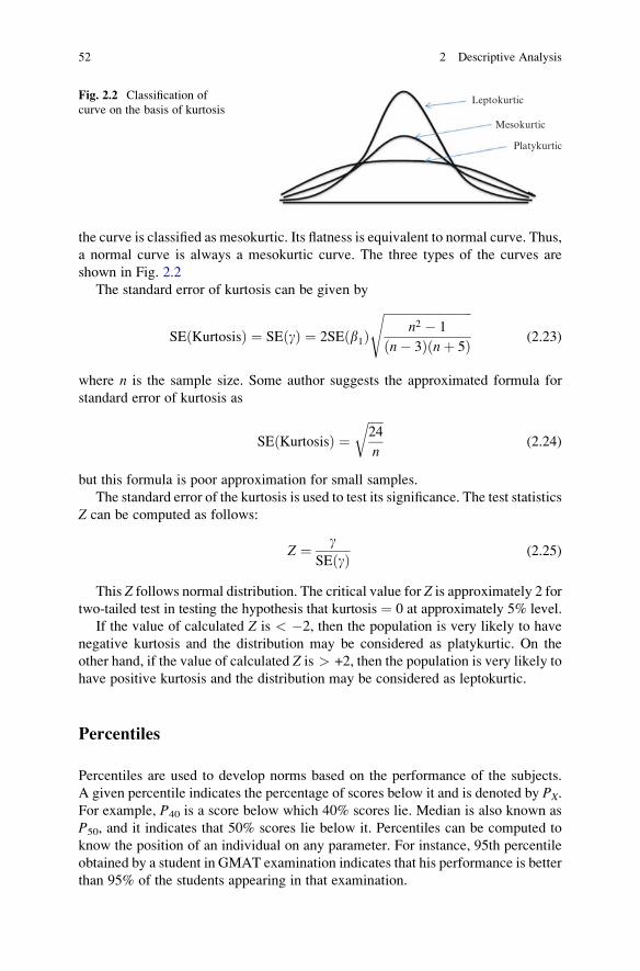
the curve is classified as mesokurtic. Its flatness is equivalent to normal curve. Thus,
a normal curve is always a mesokurtic curve. The three types of the curves are
shown in Fig. 2.2
The standard error of kurtosis can be given by
SEðKurtosisÞ ¼ SEðgÞ ¼ 2SE b1ð Þffiffiffiffiffiffiffiffiffiffiffiffiffiffiffiffiffiffiffiffiffiffiffiffiffiffiffiffiffi
n2 � 1
ðn� 3Þðnþ 5Þ
s(2.23)
where n is the sample size. Some author suggests the approximated formula for
standard error of kurtosis as
SEðKurtosisÞ ¼ffiffiffiffiffi24
n
r(2.24)
but this formula is poor approximation for small samples.
The standard error of the kurtosis is used to test its significance. The test statistics
Z can be computed as follows:
Z ¼ gSEðgÞ (2.25)
This Z follows normal distribution. The critical value for Z is approximately 2 for
two-tailed test in testing the hypothesis that kurtosis ¼ 0 at approximately 5% level.
If the value of calculated Z is < �2, then the population is very likely to have
negative kurtosis and the distribution may be considered as platykurtic. On the
other hand, if the value of calculated Z is > +2, then the population is very likely to
have positive kurtosis and the distribution may be considered as leptokurtic.
Percentiles
Percentiles are used to develop norms based on the performance of the subjects.
A given percentile indicates the percentage of scores below it and is denoted by PX.
For example, P40 is a score below which 40% scores lie. Median is also known as
P50, and it indicates that 50% scores lie below it. Percentiles can be computed to
know the position of an individual on any parameter. For instance, 95th percentile
obtained by a student in GMAT examination indicates that his performance is better
than 95% of the students appearing in that examination.
Leptokurtic
Mesokurtic
Platykurtic
Fig. 2.2 Classification of
curve on the basis of kurtosis
52 2 Descriptive Analysis

Since 25th percentile P25, 50th percentile P50, and 75th percentile P75 are also
known as first, second, and third quartiles, respectively, hence procedure of com-
puting other percentiles will be same as the procedure adopted in computing
quartiles. Quartiles (the 25th, 50th, and 75th percentiles) divide the data into four
groups of equal size. Percentiles at decile points and quartiles can be computed by
using SPSS.
Percentile Rank
A percentile rank can be defined as the percentage of scores that fall at or below a
given score. Thus, if the percentile rank of a score A is X, it indicates that Xpercentage of scores lies below the score A. The percentile rank can be computed
from the following formula:
Percentile rank of the scoreX ¼ CF� 0:5� f sn
� 100 (2.26)
where
CF: number of scores below Xfs : number of times the score X occurs in the data set
n : number of scores in the data set
Situation for Using Descriptive Study
There may be varieties of situation where a descriptive study may be planned. One
such situation has been discussed below to narrate the use of such study.
Nowadays Industries are also assuming social responsibilities toward society.
They keep engage themselves in many of the social activities like adult literacy,
slum development, HIV and AIDS program, community development, energy
conservation drive, and go green campaign. One such organization has started its
HIV and AIDS program in which it not only promotes the awareness but also
provides treatments. This company provides antiretroviral therapy to anyone in the
community who is a HIV-positive irrespective of whether that person is an
employee of the company or not. The company also provides counseling, education,
and training and disseminates information on nutrition, health, and hygiene. The
target population of the company for this program is truck drivers, contract and
migrant workers, employees of local organizations, and members of the local com-
munity. Descriptive study may be conducted to investigate the following issues:
(a) Number of programs organized in different sections of the society
(b) Number of people who attended the awareness program in different sections of
the society
Situation for Using Descriptive Study 53

(c) Number of people who are affected with HIV/AIDS in different sections of the
society
(d) The most vulnerable group affected by the HIV
(e) Details of population affected from HIV in different age and sex categories
To cater the above objectives, data may be processed as follows:
(i) Classify the data on HIV/AIDS-infected persons in different sections of the
society like truck drivers, contract laborers, migrant’s laborers, and local
establishment members of the local community month wise in the last
5 years.
(ii) Classify the number of participants attending the HIV/AIDS awareness pro-
gram in different sections of the society month wise in the last 5 years.
(iii) Compute the largest and smallest scores, mean, SD, coefficient of variation,
standard error, skewness, kurtosis, and quartile deviation for the data in all
the groups.
All these computations can be done by using SPSS, the procedure of which shall
be explained later in this chapter by using the following example:
Solved Example of Descriptive Statistics using SPSS
The procedure of computing various descriptive statistics including central ten-
dency, dispersion, percentile values, and distribution parameters through SPSS
has been explained in the solved Example 2.1.
Example 2.1 In a study conducted by response of customers were obtained on
various attributed of a company along with their satisfaction level. Apply descrip-
tive analysis to compute various statistics and explain the findings (Table 2.8).
Solution In order to compute various descriptive statistics like mean, median,
mode, SD, variance, skewness, SE of skewness, kurtosis, SE of kurtosis, range,
minimum and maximum scores, and percentiles, a data file shall be made in SPSS
and then steps shown below shall be followed to get the output. After getting the
output, its interpretation shall be made.
Computation of Descriptive Statistics Using SPSS
(a) Preparing Data FileIn order to use SPSS for computing descriptive statistics, a data file needs to be
prepared. The data file can also be imported in SPSS from the ASCII or Excel
files. The readers are advised to go through the first chapter of the book to learn
54 2 Descriptive Analysis
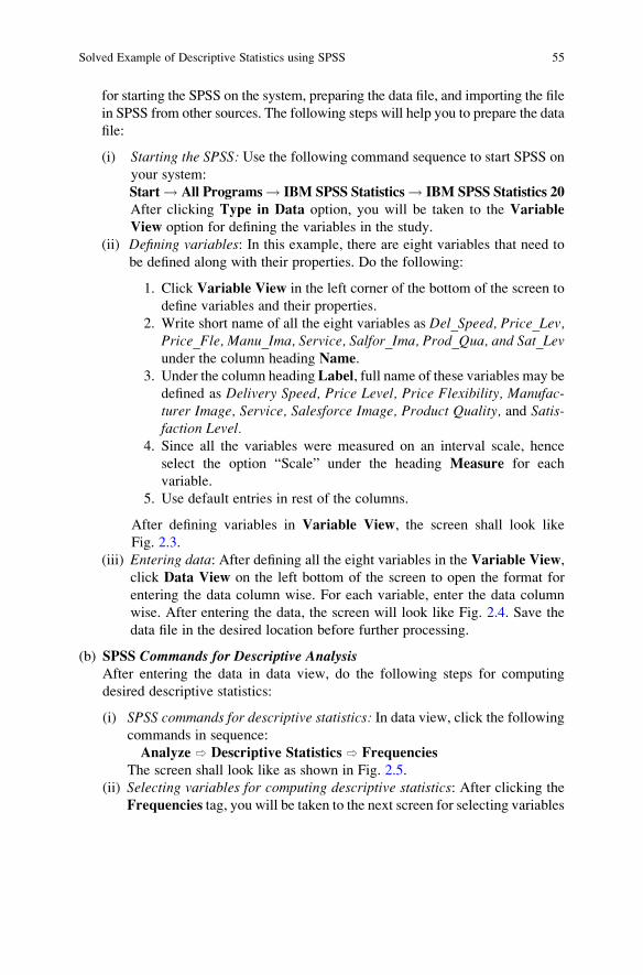
for starting the SPSS on the system, preparing the data file, and importing the file
in SPSS from other sources. The following steps will help you to prepare the data
file:
(i) Starting the SPSS: Use the following command sequence to start SPSS on
your system:
Start! All Programs! IBM SPSS Statistics! IBM SPSS Statistics 20
After clicking Type in Data option, you will be taken to the Variable
View option for defining the variables in the study.
(ii) Defining variables: In this example, there are eight variables that need to
be defined along with their properties. Do the following:
1. Click Variable View in the left corner of the bottom of the screen to
define variables and their properties.
2. Write short name of all the eight variables as Del_Speed, Price_Lev,Price_Fle, Manu_Ima, Service, Salfor_Ima, Prod_Qua, and Sat_Levunder the column heading Name.
3. Under the column heading Label, full name of these variables may be
defined as Delivery Speed, Price Level, Price Flexibility, Manufac-turer Image, Service, Salesforce Image, Product Quality, and Satis-faction Level.
4. Since all the variables were measured on an interval scale, hence
select the option “Scale” under the heading Measure for each
variable.
5. Use default entries in rest of the columns.
After defining variables in Variable View, the screen shall look like
Fig. 2.3.
(iii) Entering data: After defining all the eight variables in the Variable View,
click Data View on the left bottom of the screen to open the format for
entering the data column wise. For each variable, enter the data column
wise. After entering the data, the screen will look like Fig. 2.4. Save the
data file in the desired location before further processing.
(b) SPSS Commands for Descriptive AnalysisAfter entering the data in data view, do the following steps for computing
desired descriptive statistics:
(i) SPSS commands for descriptive statistics: In data view, click the followingcommands in sequence:
Analyze ⇨ Descriptive Statistics ⇨ Frequencies
The screen shall look like as shown in Fig. 2.5.
(ii) Selecting variables for computing descriptive statistics: After clicking the
Frequencies tag, you will be taken to the next screen for selecting variables
Solved Example of Descriptive Statistics using SPSS 55

for which descriptive statistics need to be computed. The screen shall look
like as shown in Fig. 2.6. Do the following:
– Select the variables Del_Speed, Price_Lev, Price_Fle, Manu_Ima, Ser-vice, Salfor_Ima, Prod_Qua, and Sat_Lev from the left panel to the
“Variable(s)” section of the right panel.
Here, all the eight variables can be selected one by one or all at once. To do
so, the variable(s) needs to be selected from the left panel, and by arrow
command, it may be brought to the right panel. The screen shall look like
Fig. 2.6.
(iii) Selecting option for computation: After selecting the variables, options
need to be defined for the computation of desired statistics. Do the
following:
– Click the option Statistics on the screen as shown in Fig. 2.6. This will
take you to the next screen that is shown in Fig. 2.7. Do the following:
– Check the options “Quartiles” and “Cut points for 10 equal groups”
in “Percentile Values” section.
– Check the option “Mean,” “Median,” and “Mode” under “Central
Tendency” section.
– Check the option “Std. Deviation,” “Variance,” “Range,” “Mini-
mum,” “Maximum,” “Range,” and “S.E. mean” under “Dispersion”
section.
Table 2.8 Response of customers on company’s attributes
S.
N.
Delivery
speed
(X1)
Price
level
(X2)
Price
flexibility
(X3)
Manufacturer
image (X4)
Service
(X5)
Salesforce
image (X6)
Product
quality
(X7)
Satisfaction
level (X8)
1 4.1 0.6 6.9 4.7 2.4 2.3 5.2 4.2
2 1.8 3.0 6.3 6.6 2.5 4.0 8.4 4.3
3 3.4 5.2 5.7 6.0 4.3 2.7 8.2 5.2
4 2.7 1.0 7.1 5.9 1.8 2.3 7.8 3.9
5 6.0 0.9 9.6 7.8 3.4 4.6 4.5 6.8
6 1.9 3.3 7.9 4.8 2.6 1.9 9.7 4.4
7 4.6 2.4 9.5 6.6 3.5 4.5 7.6 5.8
8 1.3 4.2 6.2 5.1 2.8 2.2 6.9 4.3
9 5.5 1.6 9.4 4.7 3.5 3.0 7.6 5.4
10 4.0 3.5 6.5 6.0 3.7 3.2 8.7 5.4
11 2.4 1.6 8.8 4.8 2.0 2.8 5.8 4.3
12 3.9 2.2 9.1 4.6 3.0 2.5 8.3 5.0
13 2.8 1.4 8.1 3.8 2.1 1.4 6.6 4.4
14 3.7 1.5 8.6 5.7 2.7 3.7 6.7 5.0
15 4.7 1.3 9.9 6.7 3.0 2.6 6.8 5.9
16 3.4 2.0 9.7 4.7 2.7 1.7 4.8 4.7
17 3.2 4.1 5.7 5.1 3.6 2.9 6.2 4.4
18 4.9 1.8 7.7 4.3 3.4 1.5 5.9 5.6
19 5.3 1.4 9.7 6.1 3.3 3.9 6.8 5.9
20 4.7 1.3 9.9 6.7 3.0 2.6 6.8 6.0
56 2 Descriptive Analysis

– Check the option “Skewness” and “Kurtosis” under “Distribution”
section.
– Click Continue for getting back to the screen shown in Fig. 2.6.
Remarks
(a) You have four different classes of statistics like “Percentile Value,”
“Central Tendency,” “Dispersion,” and “Distribution” that can be
computed. Any or all the options may be selected under these
categories. Under the category “Percentile Values,” quartiles can be
checked (√) for computing Q1 and Q3. For computing percentiles at
deciles points, cut points can be selected for 10 equal groups. Simi-
larly, if the percentiles are required to be computed in the interval of 5,
cut points may be selected as 5.
(b) In using the option cut points for the percentiles, output contains some
additional information on frequency in different segments. If the
researcher is interested, the same may be incorporated in the findings;
otherwise, it may be ignored.
(c) “Percentile” option is selected if percentile values at different
intervals are required to be computed. For example, if we are inter-
ested in computing P4, P16, P27, and P39, then these numbers are added
in the “Percentile(s)” option.
(d) In this problem, only quartiles and cut points for “10” options have
been checked under the heading “Percentile Values,” whereas under
the heading “Central Tendency,” “Dispersion,” and “Distribution,” all
the options have been checked.
(iv) Option for graph: The option Chart can be clicked in Fig. 2.6 if graph is
required to be constructed. Any one of the option under this tag like bar
charts, pie charts, or histograms may be selected. If no chart is required,
then option “None” may be selected.
Fig. 2.3 Defining variables along with their characteristics
Solved Example of Descriptive Statistics using SPSS 57

– Press O.K. for output.
(c) Getting the OutputClicking the option OK will lead you to the output window. The output panel
shall have lots of results. It is up to the researcher to select the relevant outputs
in their results. In the output window of the SPSS, the relevant output can be
selected by pressing the right click of the mouse over it and may be copied in
the word file. In this example, the output generated will look like as shown in
Table 2.9
Interpretation of the Outputs
Different interpretations can be made from the results in Table 2.9. However, some
of the important findings that can be drawn are as follows:
1. Except price level, mean and median of all the variables are nearly equal.
Fig. 2.4 Screen showing entered data for all the variables in the data view
58 2 Descriptive Analysis
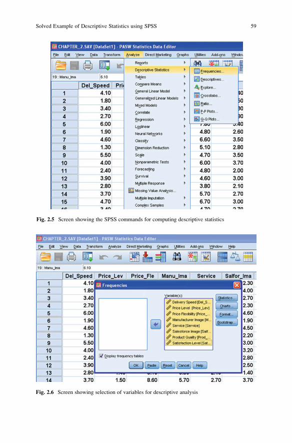
Fig. 2.6 Screen showing selection of variables for descriptive analysis
Fig. 2.5 Screen showing the SPSS commands for computing descriptive statistics
Solved Example of Descriptive Statistics using SPSS 59
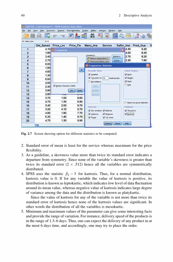
2. Standard error of mean is least for the service whereas maximum for the price
flexibility.
3. As a guideline, a skewness value more than twice its standard error indicates a
departure from symmetry. Since none of the variable’s skewness is greater than
twice its standard error (2 � .512) hence all the variables are symmetrically
distributed.
4. SPSS uses the statistic b2 � 3 for kurtosis. Thus, for a normal distribution,
kurtosis value is 0. If for any variable the value of kurtosis is positive, its
distribution is known as leptokurtic, which indicates low level of data fluctuation
around its mean value, whereas negative value of kurtosis indicates large degree
of variance among the data and the distribution is known as platykurtic.
Since the value of kurtosis for any of the variable is not more than twice its
standard error of kurtosis hence none of the kurtosis values are significant. In
other words the distribution of all the variables is mesokurtic.
5. Minimum and maximum values of the parameter can give some interesting facts
and provide the range of variation. For instance, delivery speed of the products is
in the range of 1.3–6 days. Thus, one can expect the delivery of any product in at
the most 6 days time, and accordingly, one may try to place the order.
Fig. 2.7 Screen showing option for different statistics to be computed
60 2 Descriptive Analysis

Table
2.9
Outputshowingvariousstatistics
fordifferentattributesofthecompany
Del_Speed
Price_Lev
Price_Fle
Manu_Im
aService
Salfor_Im
aProd_Qua
Sat_Lev
NValid
20
20
20
20
20
20
20
20
Missing
00
00
00
00
Mean
3.7150
2.2150
8.1150
5.5350
2.9650
2.8150
6.9650
5.0450
SEofmean
.29094
.28184
.33563
.22933
.14203
.20841
.30177
.17524
Median
3.8000
1.7000
8.3500
5.4000
3.0000
2.6500
6.8000
5.0000
Mode
3.40a
1.30a
5.70a
4.70
3.00
2.30a
6.80
4.30a
Std.deviation
1.30112
1.26044
1.50097
1.02561
.63518
.93205
1.34957
.78370
Variance
1.693
1.589
2.253
1.052
.403
.869
1.821
.614
Skew
ness
�.144
.970
�.338
.380
.010
.459
.001
.490
SEofskew
ness
.512
.512
.512
.512
.512
.512
.512
.512
Kurtosis
�.732
.092
�1.435
�.467
�.288
�.500
�.324
�.566
SEofkurtosis
.992
.992
.992
.992
.992
.992
.992
.992
Range
4.70
4.60
4.20
4.00
2.50
3.20
5.20
2.90
Minim
um
1.30
.60
5.70
3.80
1.80
1.40
4.50
3.90
Maxim
um
6.00
5.20
9.90
7.80
4.30
4.60
9.70
6.80
Sum
74.30
44.30
162.30
110.70
59.30
56.30
139.30
100.90
Percentiles
10
1.8100
.9100
5.7500
4.3300
2.0100
1.5200
4.8400
4.2100
20
2.4600
1.3000
6.3400
4.7000
2.4200
1.9600
5.8200
4.3000
25
2.7250
1.3250
6.6000
4.7000
2.5250
2.2250
5.9750
4.3250
30
2.9200
1.4000
6.9600
4.7300
2.6300
2.3000
6.3200
4.4000
40
3.4000
1.5400
7.7800
4.9200
2.7400
2.5400
6.7400
4.5200
50
3.8000
1.7000
8.3500
5.4000
3.0000
2.6500
6.8000
5.0000
60
4.0600
2.1200
8.9800
5.9600
3.1800
2.8600
7.3200
5.3200
70
4.6700
2.8200
9.4700
6.0700
3.4000
3.1400
7.7400
5.5400
75
4.7000
3.2250
9.5750
6.4750
3.4750
3.5750
8.1000
5.7500
80
4.8600
3.4600
9.6800
6.6000
3.5000
3.8600
8.2800
5.8800
90
5.4800
4.1900
9.8800
6.7000
3.6900
4.4500
8.6700
5.9900
aMultiple
modes
exist.Thesm
allestvalueisshown
Del_Sp
eeddeliveryspeed,Price_Lev
price
level,Price_F
leprice
flexibility,Man
u_Im
amanufacturerim
age,Serviceservice,Sa
lfor_Imasalesforceim
age,
Prod_Q
uaproduct
quality,Sa
t_Lev
satisfactionlevel
Solved Example of Descriptive Statistics using SPSS 61
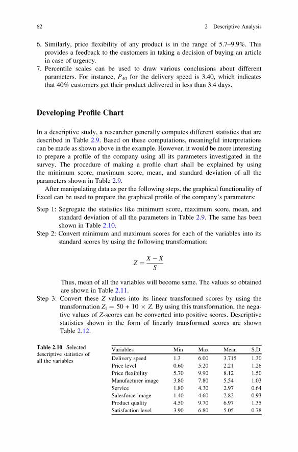
6. Similarly, price flexibility of any product is in the range of 5.7–9.9%. This
provides a feedback to the customers in taking a decision of buying an article
in case of urgency.
7. Percentile scales can be used to draw various conclusions about different
parameters. For instance, P40 for the delivery speed is 3.40, which indicates
that 40% customers get their product delivered in less than 3.4 days.
Developing Profile Chart
In a descriptive study, a researcher generally computes different statistics that are
described in Table 2.9. Based on these computations, meaningful interpretations
can be made as shown above in the example. However, it would be more interesting
to prepare a profile of the company using all its parameters investigated in the
survey. The procedure of making a profile chart shall be explained by using
the minimum score, maximum score, mean, and standard deviation of all the
parameters shown in Table 2.9.
After manipulating data as per the following steps, the graphical functionality of
Excel can be used to prepare the graphical profile of the company’s parameters:
Step 1: Segregate the statistics like minimum score, maximum score, mean, and
standard deviation of all the parameters in Table 2.9. The same has been
shown in Table 2.10.
Step 2: Convert minimum and maximum scores for each of the variables into its
standard scores by using the following transformation:
Z ¼ X � �X
S
Thus, mean of all the variables will become same. The values so obtained
are shown in Table 2.11.
Step 3: Convert these Z values into its linear transformed scores by using the
transformation Zl ¼ 50 + 10 � Z. By using this transformation, the nega-
tive values of Z-scores can be converted into positive scores. Descriptive
statistics shown in the form of linearly transformed scores are shown
Table 2.12.
Table 2.10 Selected
descriptive statistics of
all the variables
Variables Min Max Mean S.D.
Delivery speed 1.3 6.00 3.715 1.30
Price level 0.60 5.20 2.21 1.26
Price flexibility 5.70 9.90 8.12 1.50
Manufacturer image 3.80 7.80 5.54 1.03
Service 1.80 4.30 2.97 0.64
Salesforce image 1.40 4.60 2.82 0.93
Product quality 4.50 9.70 6.97 1.35
Satisfaction level 3.90 6.80 5.05 0.78
62 2 Descriptive Analysis
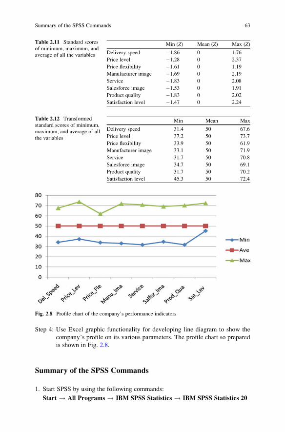
Step 4: Use Excel graphic functionality for developing line diagram to show the
company’s profile on its various parameters. The profile chart so prepared
is shown in Fig. 2.8.
Summary of the SPSS Commands
1. Start SPSS by using the following commands:
Start ! All Programs ! IBM SPSS Statistics ! IBM SPSS Statistics 20
Table 2.11 Standard scores
of minimum, maximum, and
average of all the variables
Min (Z) Mean (Z) Max (Z)
Delivery speed �1.86 0 1.76
Price level �1.28 0 2.37
Price flexibility �1.61 0 1.19
Manufacturer image �1.69 0 2.19
Service �1.83 0 2.08
Salesforce image �1.53 0 1.91
Product quality �1.83 0 2.02
Satisfaction level �1.47 0 2.24
Table 2.12 Transformed
standard scores of minimum,
maximum, and average of all
the variables
Min Mean Max
Delivery speed 31.4 50 67.6
Price level 37.2 50 73.7
Price flexibility 33.9 50 61.9
Manufacturer image 33.1 50 71.9
Service 31.7 50 70.8
Salesforce image 34.7 50 69.1
Product quality 31.7 50 70.2
Satisfaction level 45.3 50 72.4
Fig. 2.8 Profile chart of the company’s performance indicators
Summary of the SPSS Commands 63
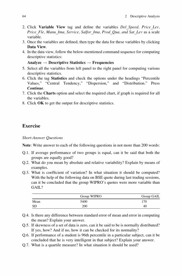
2. Click Variable View tag and define the variables Del_Speed, Price_Lev,Price_Fle, Manu_Ima, Service, Salfor_Ima, Prod_Qua, and Sat_Lev as a scalevariable.
3. Once the variables are defined, then type the data for these variables by clicking
Data View.
4. In the data view, follow the below-mentioned command sequence for computing
descriptive statistics:
Analyze ! Descriptive Statistics ! Frequencies
5. Select all the variables from left panel to the right panel for computing various
descriptive statistics.
6. Click the tag Statistics and check the options under the headings “Percentile
Values,” “Central Tendency,” “Dispersion,” and “Distribution.” Press
Continue.7. Click the Charts option and select the required chart, if graph is required for all
the variables.
8. Click OK to get the output for descriptive statistics.
Exercise
Short-Answer Questions
Note: Write answer to each of the following questions in not more than 200 words:
Q.1. If average performance of two groups is equal, can it be said that both the
groups are equally good?
Q.2. What do you mean by absolute and relative variability? Explain by means of
examples.
Q.3. What is coefficient of variation? In what situation it should be computed?
With the help of the following data on BSE quote during last trading sessions,
can it be concluded that the group WIPRO’s quotes were more variable than
GAIL?
Group WIPRO Group GAIL
Mean 5400 170
SD 200 40
Q.4. Is there any difference between standard error of mean and error in computing
the mean? Explain your answer.
Q.5. If skewness of a set of data is zero, can it be said to be is normally distributed?
If yes, how? And if no, how it can be checked for its normality?
Q.6. If performance of a student is 96th percentile in a particular subject, can it be
concluded that he is very intelligent in that subject? Explain your answer.
Q.7. What is a quartile measure? In what situation it should be used?
64 2 Descriptive Analysis
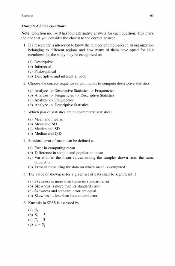
Multiple-Choice Questions
Note: Question no. 1–10 has four alternative answers for each question. Tick mark
the one that you consider the closest to the correct answer.
1. If a researcher is interested to know the number of employees in an organization
belonging to different regions and how many of them have opted for club
memberships, the study may be categorized as
(a) Descriptive
(b) Inferential
(c) Philosophical
(d) Descriptive and inferential both
2. Choose the correct sequence of commands to compute descriptive statistics.
(a) Analyze -> Descriptive Statistics -> Frequencies
(b) Analyze -> Frequencies -> Descriptive Statistics
(c) Analyze -> Frequencies
(d) Analyze -> Descriptive Statistics
3. Which pair of statistics are nonparametric statistics?
(a) Mean and median
(b) Mean and SD
(c) Median and SD
(d) Median and Q.D.
4. Standard error of mean can be defined as
(a) Error in computing mean
(b) Difference in sample and population mean
(c) Variation in the mean values among the samples drawn from the same
population
(d) Error in measuring the data on which mean is computed
5. The value of skewness for a given set of data shall be significant if
(a) Skewness is more than twice its standard error.
(b) Skewness is more than its standard error.
(c) Skewness and standard error are equal.
(d) Skewness is less than its standard error.
6. Kurtosis in SPSS is assessed by
(a) b2(b) b2 þ 3
(c) b2 � 3
(d) 2þ b2
Exercise 65

7. In order to prepare the profile chart, minimum scores for each variable are
converted into
(a) Percentage
(b) Standard score
(c) Percentile score
(d) Rank
8. While selecting option for percentile in SPSS, cut points are used for
(a) Computing Q1 and Q3
(b) Preparing the percentile at deciles points only
(c) Cutting Q1 and Q3
(d) Computing the percentiles at fixed interval points
9. If IQ of a group of students is positively skewed, what conclusions could be
drawn?
(a) Most of the students are less intelligent.
(b) Most of the students are more intelligent.
(c) There are equal number of high and low intelligent students.
(d) Nothing can be said about the intelligence of the students.
10. If the data is platykurtic, what can be said about its variability?
(a) More variability exists.
(b) Less variability exists.
(c) Variability is equivalent to normal distribution.
(d) Nothing can be said about the variability.
Assignment
1. Following table shows the data on different abilities of employees in an organi-
zation. Compute various descriptive statistics and interpret its findings.
Data on different abilities of employees
Define
problems
Supervise
others
Make
decisions
Build
consensus
Facilitate decision-
making
Work on a
team
.81 .84 .80 .89 .79 .72
.45 .31 .29 .37 .21 .12
.87 .79 .90 .88 .67 .50
.78 .71 .84 .92 .82 .62
.65 .59 .72 .85 .81 .56
.56 .55 .62 .71 .73 .61
66 2 Descriptive Analysis

2. Following are the grades of ten MBA students in 10 courses. Compute various
descriptive statistics and interpret your findings.
Answers of Multiple-Choice Questions
Q.1 a Q.2 a
Q.3 d Q.4 c
Q.5 a Q.6 c
Q.7 b Q.8 d
Q.9 a Q.10 a
Data on grades of MBA students in ten courses
S.N. FACTG MACTG ECON FIN MKTG ENVIR MIS QM OPSM OB
1 7 1 7 6 6 6 7 5 5 6
2 7 6 7 7 6 5 6 7 4 7
3 3 6 6 6 6 4 5 4 6 7
4 8 7 8 6 7 8 7 8 9 6
5 5 3 5 7 5 8 6 6 4 8
6 3 3 3 3 3 5 6 7 7 7
7 4 7 6 5 8 6 5 4 4 6
8 5 6 8 7 6 7 8 7 5 5
9 6 5 7 8 5 6 5 8 7 7
10 7 6 5 8 6 4 8 6 7 8
FACTG financial accounting for managers, MACTG management accounting, ECON economic
environment of business, FINE managerial finance, MKTG marketing management, NVIR busi-
ness environment, MIS management information systems, QM quantitative methods, OPSMoperations management, OB organizational behavior
Exercise 67

Chapter 3
Chi-Square Test and Its Application
Learning Objectives
After completing this chapter you should be able to do the following:
• Know the use of chi-square in analyzing nonparametric data.
• Understand the application of chi-square in different research situations.
• Know the advantages of crosstabs analysis.
• Learn to construct the hypothesis in applying chi-square test.
• Explain the situations in which different statistics like contingency coefficient,
lambda coefficient, phi coefficient, gamma, Cramer’s V, and Kendall tau, for
measuring an association between two attributes, can be used.
• Learn the procedure of data feeding in preparing the data file for analysis using SPSS.
• Describe the procedure of testing an equal occurrence hypothesis and testing the
significance of an association in different applications by using SPSS.
• Interpret the output of chi-square analysis generated in SPSS.
Introduction
In survey research, mainly two types of hypothesis are tested. One may test goodness
of fit for a single attribute or may like to test the significance of association between
any two attributes. To test an equal occurrence hypothesis, it is required to tabulate
the observed frequency for each variable. The chi-square statistic in “nonparametric”
section of SPSS may be used to test the hypothesis of equal occurrence.
The scores need to be arranged in contingency table for studying an association
between any two attributes. A contingency table is the arrangement of frequency in
rows and column. The process of creating a contingency table from the observed
frequency is known as crosstab. The cross tabulation procedure provides tabulation of
two variables in two-way table. A frequency distribution provides the distribution of
one variable, whereas a contingency table describes the distribution of two or more
variables simultaneously (Table 3.1).
J.P. Verma, Data Analysis in Management with SPSS Software,DOI 10.1007/978-81-322-0786-3_3, # Springer India 2013
69

The following is an example of a 2 � 3 contingency table. The first variable
“gender” has two options, male and female, whereas the second variable
“incentives” has three options, gift check, cash, and gift article. Each cell gives
the number of individuals who share the combination of traits.
The chi-square can be computed by using the Crosstabs option in “Descriptive
Statistics” section of SPSS command. Besides chi-square, the Crosstabs option in
SPSS provides the output showing magnitude of association along with summary
statistics including percentage of frequency and expected frequency in each cell.
Two-way tabulation in Crosstabs can be used to establish an interdependent
relationship between two tables of values but does not identify a causal relation
between the values. Cross tabulation technique can be used to analyze the results of
a survey study, for example, it may indicate a preference for certain types of jobs
based on the respondent’s gender.
Advantages of Using Crosstabs
1. Crosstabs analysis is easy to understand and is good for the researchers, who do
not want to use more sophisticated statistical techniques.
2. Crosstabs treats all data as nominal. In other words, the data is treated as nominal
even if it is measured in interval, ratio, or ordinal form.
3. A table is more explanatory than a single statistics.
4. They are simple to conduct.
Statistics Used in Cross Tabulations
In Crosstabs analysis, usually statistics like chi-square, contingency coefficient,
lambda coefficient, phi coefficient, Kendall tau, gamma, or Cramer’s V are used.
These shall be discussed below:
Chi-Square Statistic
If X1, . . ., Xn are independent and identical N(m, s2) random variables, then the
statisticsPni¼1
Xi�m:s
� �2follows the chi-square distribution with (n�1) degrees of
freedom and is written as
Table 3.1 Preferences of
male and female towards
different incentives
Incentives
Gift check (%) Cash (%) Gift article (%)
Gender Male 30 45 25
Female 10 30 60
70 3 Chi-Square Test and Its Application

Xni¼1
Xi � ms
� �2
� w2 n� 1ð Þ
The probability density function of the chi-square (w2) random variable is
f ðxÞ ¼ 1
2n=2G n=2ð Þ xn=2�1e�x=2 (3.1)
x>0 and n ¼ 1; 2; 3; . . .
The mean and variance of the chi-square statistics are n and 2n, respectively. Thew2 distribution is not unique but depends upon degrees of freedom. The family of
distribution with varying degrees of freedom is shown in Fig. 3.1.
Additive Properties of Chi-Square
If w21 and w22 are two independent chi-square variates with n1 and n2 degrees of
freedom, respectively, then w21 + w22 is also a chi-square variate with n1 + n2 degreesof freedom. This property is used extensively in the questionnaire studies. Consider
a study to compare the attitude of male and female consumers about a particular
brand of car. The questionnaire may consist of questions under three factors,
namely, financial consideration, driving comforts, and facilities. Each of these
factors may have several questions. On each of the questions, attitude of male
and female users may be compared using chi-square. Further, by using additive
n=1
n=2
n=3
n=4 n=50.
4
p(x)
0.2
0.0
0.6
0.8
1.0
0
3
5
2
1
2 4
x
6 8
4
Fig. 3.1 Probability
distribution of chi-square for
different degrees of freedom
Statistics Used in Cross Tabulations 71
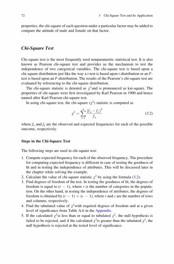
properties, the chi-square of each question under a particular factor may be added to
compare the attitude of male and female on that factor.
Chi-Square Test
Chi-square test is the most frequently used nonparametric statistical test. It is also
known as Pearson chi-square test and provides us the mechanism to test the
independence of two categorical variables. The chi-square test is based upon a
chi-square distribution just like the way a t-test is based upon t-distribution or an F-test is based upon an F-distribution. The results of the Pearson’s chi-square test areevaluated by referencing to the chi-square distribution.
The chi-square statistic is denoted as w2 and is pronounced as kai-square. The
properties of chi-square were first investigated by Karl Pearson in 1900 and hence
named after Karl Pearson chi-square test.
In using chi-square test, the chi-square (w2) statistic is computed as
w2 ¼Xni¼1
ðf o � f eÞ2f e
(3.2)
where fo and fe are the observed and expected frequencies for each of the possible
outcome, respectively.
Steps in the Chi-Square Test
The following steps are used in chi-square test:
1. Compute expected frequency for each of the observed frequency. The procedure
for computing expected frequency is different in case of testing the goodness of
fit and in testing the independence of attributes. This will be discussed later in
the chapter while solving the example.
2. Calculate the value of chi-square statistic w2 by using the formula (3.2).
3. Find degrees of freedom of the test. In testing the goodness of fit, the degrees of
freedom is equal to (r � 1), where r is the number of categories in the popula-
tion. On the other hand, in testing the independence of attributes, the degrees of
freedom is obtained by (r � 1) � (c � 1), where r and c are the number of rows
and columns, respectively.
4. Find the tabulated value of w2with required degrees of freedom and at a given
level of significance from Table A.6 in the Appendix.
5. If the calculated w2 is less than or equal to tabulated w2 , the null hypothesis is
failed to be rejected, and if the calculated w2is greater than the tabulated w2, thenull hypothesis is rejected at the tested level of significance.
72 3 Chi-Square Test and Its Application
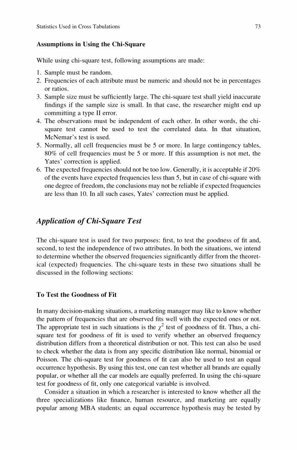
Assumptions in Using the Chi-Square
While using chi-square test, following assumptions are made:
1. Sample must be random.
2. Frequencies of each attribute must be numeric and should not be in percentages
or ratios.
3. Sample size must be sufficiently large. The chi-square test shall yield inaccurate
findings if the sample size is small. In that case, the researcher might end up
committing a type II error.
4. The observations must be independent of each other. In other words, the chi-
square test cannot be used to test the correlated data. In that situation,
McNemar’s test is used.
5. Normally, all cell frequencies must be 5 or more. In large contingency tables,
80% of cell frequencies must be 5 or more. If this assumption is not met, the
Yates’ correction is applied.
6. The expected frequencies should not be too low. Generally, it is acceptable if 20%
of the events have expected frequencies less than 5, but in case of chi-square with
one degree of freedom, the conclusions may not be reliable if expected frequencies
are less than 10. In all such cases, Yates’ correction must be applied.
Application of Chi-Square Test
The chi-square test is used for two purposes: first, to test the goodness of fit and,
second, to test the independence of two attributes. In both the situations, we intend
to determine whether the observed frequencies significantly differ from the theoret-
ical (expected) frequencies. The chi-square tests in these two situations shall be
discussed in the following sections:
To Test the Goodness of Fit
In many decision-making situations, a marketing manager may like to know whether
the pattern of frequencies that are observed fits well with the expected ones or not.
The appropriate test in such situations is the w2 test of goodness of fit. Thus, a chi-
square test for goodness of fit is used to verify whether an observed frequency
distribution differs from a theoretical distribution or not. This test can also be used
to check whether the data is from any specific distribution like normal, binomial or
Poisson. The chi-square test for goodness of fit can also be used to test an equal
occurrence hypothesis. By using this test, one can test whether all brands are equally
popular, or whether all the car models are equally preferred. In using the chi-square
test for goodness of fit, only one categorical variable is involved.
Consider a situation in which a researcher is interested to know whether all the
three specializations like finance, human resource, and marketing are equally
popular among MBA students; an equal occurrence hypothesis may be tested by
Statistics Used in Cross Tabulations 73

computing the chi-square. The “Nonparametric Tests” option in SPSS provides the
computation of chi-square (w2). In such situations, following set of hypotheses is
tested:
H0: All three specializations are equally popular.
H1: All three specializations are not equally popular.
By using the procedure discussed above for applying chi-square test, the null
hypothesis may be tested. The procedure would clear by looking to the following
solved examples:
Example 3.1 A beverages company produces cold drink with three different
colors. One hundred and twenty college students were asked about their
preferences. The responses are shown in Table 3.2. Do these data show that all
the flavors were equally liked by the students? Test your hypothesis at .05 level of
significance.
Solution Here it is required to test the null hypothesis of equal occurrence; hence,
expected frequencies corresponding to each of the three observed frequencies shall
be obtained by dividing the total of all the observed frequencies by the number of
categories. Hence, expected frequency (fe) for each category shall be (Table 3.3)
f e ¼50þ 40þ 30
3¼ 40
Here, number of categories or rows (r) ¼ 3 and number of columns (c) ¼ 2.
w2 ¼Xri¼1
ðf o � f eÞ2f e
¼ 50� 40ð Þ240
þ 40� 40ð Þ240
þ 30� 40ð Þ240
¼ 100
40þ 0þ 100
40¼ 2:5þ 2:5
) Cal: w2 ¼ 5:0
Table 3.2 Preferences of the college students about different brands of cold drinks
Color White Orange Brown
Frequencies 50 40 30
Table 3.3 Observed and
expected frequencies of
responses
Observed frequencies Expected frequencies
(fo) (fe)
White 50 40
Orange 40 40
Brown 30 40
74 3 Chi-Square Test and Its Application

Testing the Significance of Chi-SquareThe degrees of freedom ¼ (r�1) ¼ 3�1 ¼ 2.
From Table A.6 in the Appendix, the tab w2:05ð2Þ ¼ 5:991:
Since Cal. w2 < Tab. w2:05ð2Þ, the null hypothesis may not be rejected at .05 level
of significance. Thus, it may be concluded that all the three colors of cold drinks are
equally liked by the college students.
Example 3.2 An examination was undertaken by 300 students, out of which 90
students had grade A, 65 got grade B, 60 got grade C, and the remaining had grade
D. Do these figures commensurate with the final examination result which is in the
ratio of 3:2:3:4 for various grades, respectively? Test the hypothesis at 5% level.
Solution The null hypothesis which is required to be tested here is
H0: The students in the various grades were distributed in the ratio 3:2:3:4
The expected number of students (fe) for each grade under the assumption that
H0 is true is as follows:
Expected number of students getting gradeA ¼ 3
3þ 2þ 3þ 4� 300 ¼ 75
Expected number of students getting grade B ¼ 2
12� 300 ¼ 50
Expected number of students getting grade C ¼ 3
12� 300 ¼ 75
Expected number of students getting gradeD ¼ 4
12� 300 ¼ 100
Thus, the observed and expected frequencies can be listed as shown in Table 3.4.
w2 ¼Xri¼1
ðf o � f eÞ2f e
¼ 90� 75ð Þ275
þ 65� 50ð Þ250
þ 60� 75ð Þ275
þ 85� 100ð Þ2100
¼ 225
75þ 225
50þ 225
75þ 225
100¼ 3þ 4:5þ 3þ 2:25 ¼ 12:75
) Calculated w2 ¼12:75
Table 3.4 Observed and
expected frequenciesObserved frequencies Expected frequencies
(fo) (fe)
Grade A 90 75
Grade B 65 50
Grade C 60 75
Grade D 85 100
Statistics Used in Cross Tabulations 75

Testing the Significance of Chi-SquareDegrees of freedom: (r � 1) 4�1 ¼ 3.
From Table A.6 in the Appendix, the tab w2:05ð3Þ ¼ 7:815.
Since Cal. w2 > Tab. w2:05ð3Þ, the null hypothesis may be rejected at .05 level of
significance. It may thus be concluded that grades A, B, C, and D are not in
proportion to 3:2:3:4.
To Test the Independence of Attributes
The chi-square test of independence is used to know whether paired observations on
two attributes, expressed in a contingency table, are independent of each other.
There may be varieties of situations where chi-square test of independence may be
used. For instance one may test the significance of association between income
level & brand preference, family size & television size purchased or educational
background & the type of job one does. Thus, chi-square test may be used to test the
significance of an association between any two attributes.
Let us assume that the population can be classified into r mutually exclusive
classes A1, A2,. . ., Ar on the basis of attribute A, and each of these r classes are
further classified into c mutually exclusive classes, like AiB1, AiB2, . . ., AiBc, etc.
If f oijis the observed frequency of AiBj, that is, (AiBj) ¼ f oij, the above classifica-
tion can be shown in the following table known as contingency table.
B
B1 B2 . . . Bc TotalA
A1 f o11 f o12 . . . f o1c (A1)
A2 f o21 f o22 . . . f o2c (A2)
.
.
Ar f or1 f or2 . . . f orc (Ar)
Total (B1) (B2) . . . (Bc) N
By assuming A and B as independent attributes, the expected frequencies of each
cell can be computed as
Eij ¼ ðAiÞðBjÞN
Thus,
w2 ¼Xri¼1
Xcj¼1
f oij � f eij
� �2f eij
(3.3)
shall be a w2 variate with (r � 1)(c � 1) degrees of freedom.
76 3 Chi-Square Test and Its Application

The value of the w2 variate so obtained can be used to test the independence of
two attributes.
Consider a situation where it is required to test the significance of association
between Gender (male and female) and Response (“prefer day shift” and “prefer
night shift”). In this situation, following hypotheses may be tested:
H0: Gender and Response toward shift preferences are independent.
H1: There is an association between the Gender and Response toward shift
preferences.
The calculated value of chi-square (w2) obtained from the formula (3.3) may be
compared with that of its tabulated value for testing the null hypothesis.
Thus, if calculated w2 is less than tabulated w2 with (r � 1) (c � 1) df at some
level of significance, then H0 may not be rejected otherwise H0 may be rejected.
Remark If H0 is rejected, we may interpret that there is a significant association
between the gender and their preferences toward shifts. Here, significant associa-
tion simply means that the response pattern of male and female is different. The
readers may note that chi-square statistic is used to test the significance of associa-
tion, but ultimately one gets the comparison between the levels of one attribute
across the levels of other attribute.
Example 3.3 Five hundred families were investigated to test the belief that high-
income people usually prefer to visit private hospitals and low-income people often
go to government hospitals whenever they fall sick. The results so obtained are
shown in Table 3.5.
Test whether income and hospital preferences are independent. Compute the
contingency coefficient to find the strength of association. Test your hypothesis at
5% level.
Solution The null hypothesis to be tested is
H0: Income and hospital preferences are independent.
Before computing the value of chi-square, the expected frequencies for each cell
need to be computed with the marginal totals and grand totals given in the observed
frequency (fo) table. The procedure is discussed in Table 3.6.
w2 ¼Xri¼1
Xcj¼1
f oij � f eij
� �2f eij
¼ 125� 140:4ð Þ2140:4
þ 145� 129:6ð Þ2129:6
þ 135� 119:6ð Þ2119:6
þ 95� 110:4ð Þ2110:4
¼ 1:69þ 1:83þ 1:98þ 2:15 ¼ 7:65
) Calculated w2 ¼ 7:65
Statistics Used in Cross Tabulations 77

Test of SignificanceHere, r ¼ 2 and c ¼ 2, and therefore degree of freedom is
(r � 1) � (c � 1) ¼ 1.
From Table A.6 in the Appendix, the tab w2:05ð1Þ ¼ 3:841:
Since Cal. w2 > Tab. w2:05ð1Þ, the null hypothesis may be rejected at .05 level of
significance. It may therefore be concluded that there is an association between the
income level and the types of hospital preferred by the people.
Precautions in Using the Chi-Square Test
(a) While using chi-square test, one must ensure that the sample is random,
representative, and adequate in size.
(b) Chi-square should not be calculated if the frequencies are in percentage form;
in that case, these frequencies must be converted back to absolute numbers
before using the test.
(c) If any of the cell frequencies is less than 5, then for each cell, .5 is subtracted
from the difference of observed and expected frequency while computing chi-
square. This correction is known as Yates’ correction. SPSS automatically does
this correction while computing chi-square.
(d) The sum of the observed frequencies should be equal to the sum of the expected
frequencies.
Testing the Significance of Chi-Square in SPSS
(a) In SPSS, the null hypothesis is not tested on the basis of the comparison
between calculated and tabulated chi-square; rather, it uses the concept of
p value. p value is the probability of rejecting the null hypothesis when actuallyit is true.
Table 3.5 Observed
frequencies (fo) of responsesHospitals
Government Private TotalIncome
High 125 145 270
Low 135 95 230
Total 260 240 500
Table 3.6 Expected
frequencies (fe) of responsesHospitals
Government Private TotalIncome
High 270�260500
¼ 140:4 270�240500
¼ 129:6 270
Low 230�260500
¼ 119:6 230�240500
¼ 110:4 230
Total 260 240 500
78 3 Chi-Square Test and Its Application

(b) Thus, the chi-square is said to be significant at 5% level if the p value is less
than .05 and is insignificant if it is more than .05.
Contingency Coefficient
Contingency coefficient (C) provides the magnitude of association between the
attributes in the cross tabulation. Its value can range from 0 (no association) to 1
(the theoretical maximum possible association). Chi-square simply tests the signifi-
cance of an association between any two attributes but does not provide the
magnitude of the association. Thus, if the chi-square value becomes significant,
one must compute the contingency coefficient (C) to know the extent of association
between the attributes. The contingency coefficient C is computed by the following
formula:
C ¼ffiffiffiffiffiffiffiffiffiffiffiffiffiffiw2
w2 þ N
s(3.4)
where N is the sum of all frequencies in the contingency table.
Lambda Coefficient
Lambda coefficient is used to test the strength of an association in the cross
tabulation. It is assumed that the variables are measured at the nominal level.
Lambda can have the value in the range 0 (no association) to 1 (the theoretical
maximum possible association). Asymmetric lambda measures the percentage
improvement in predicting the dependent variable. Symmetric lambda measures
the percentage improvement when prediction is done in both directions.
Phi Coefficient
In a situation when both the variables are binary, phi coefficient is used to measure
the degree of association between them. This measure is similar to the correlation
coefficient in its interpretation. Two binary variables are considered positively
associated if most of the data falls along the diagonal cells. In contrast, two binary
variables are considered negatively associated if most of the data falls off the
diagonal.
The assumptions of normality and homogeneity can be violated when the
categories are extremely uneven, as in the case of proportions close to .90, .95 or
Statistics Used in Cross Tabulations 79

.10, .05. In such cases, the phi coefficient can be significantly attenuated. The
assumption of linearity cannot be violated within the context of the phi coefficient
of correlation.
Gamma
If both the variables are measured at the ordinal level,Gamma is used for testing thestrength of association of the cross tabulations. It makes no adjustment for either
table size or ties. The value of Gamma can range from �1 (100% negative
association, or perfect inversion) to +1 (100% positive association, or perfect
agreement). A value of zero indicates the absence of association.
Cramer’s V
It measures the strength of association between attributes in cross tabulations. It is a
variant of the phi coefficient that adjusts for the number of rows and columns. Its
value can range from 0 (no association) to 1 (the theoretical maximum possible
association).
Kendall Tau
Tau b and Tau c both test the strength of association of the cross tabulations in a
situation when both variables are measured at the ordinal level. Both these tests Taub and Tau c make adjustments for ties, but Tau b is most suitable for square tables
whereas Tau c is most suitable for rectangular tables. Their values can range from
�1 (100% negative association, or perfect inversion) to +1 (100% positive associa-
tion, or perfect agreement). A value of zero indicates the absence of association.
Situation for Using Chi-Square
Chi-square is one of the most popularly used nonparametric statistical tests used in
the questionnaire study. Two different types of hypotheses, that is, testing the
goodness of fit and testing the significance of association between two attributes,
can be tested using chi-square.
Testing an equal occurrence hypothesis is a special case of goodness of fit.
In testing an equal occurrence hypothesis, the observed frequencies on different
80 3 Chi-Square Test and Its Application

levels of a factor are obtained. The total of observed frequencies for all the levels is
divided by the number of levels to obtain the expected frequencies for each level.
Consider an experiment in which it is intended to test whether all the three
locations, that is, Delhi, Mumbai, and Chennai, are equally preferred by the
employees of an organization for posting. Out of 250 employees surveyed, 120
preferred Delhi, 80 preferred Mumbai, and 50 preferred Chennai. In this situation,
the following null hypothesis may be tested using chi-square:
H0: All the three locations are equally preferred.
Against the alternative hypothesis:
H1: All the three locations are not equally preferred.
Here, the chi-square test can be used to test the null hypothesis of equal
occurrence.
Another application of chi-square is to test the significance of association between
any two attributes. Suppose it is desired to know as to whether preference of
consumers for a specific brand of soap depends upon their socioeconomic status
where the response of 200 customers is shown in Table 3.7.
The following null hypothesis may be tested by using the chi-square for two
samples at 5% level to answer the question.
H0: Socioeconomic status and soap preferences are independent.
Against the alternative hypothesis:
H1: There is an association between the socioeconomic status and soap preferences.
If the null hypothesis is rejected, one may draw the conclusion that the prefer-
ence of soap is significantly associated with the socioeconomic status of an individ-
ual. In other words, it may be concluded that the response patterns of the customers
in high and low socioeconomic status are different.
The above two different kinds of application of chi-square have been discussed
below by means of solved examples using SPSS.
Solved Examples of Chi-square for Testing an Equal
Occurrence Hypothesis
Example 3.4 In a study, 90 workers were tested for their job satisfaction. Their job
satisfaction level was obtained on the basis of the questionnaire, and the
respondents were classified into one of the three categories, namely, low, average,
and high. The observed frequencies are shown in Table 3.8. Compute chi-square in
testing whether there is any specific trend in their job satisfaction.
Table 3.7 Observed
frequencies in a contingency
table Socioeconomic status
Category of preference
Prefer Do not prefer
High 80 15
Low 40 65
Solved Examples of Chi-square for Testing an Equal Occurrence Hypothesis 81
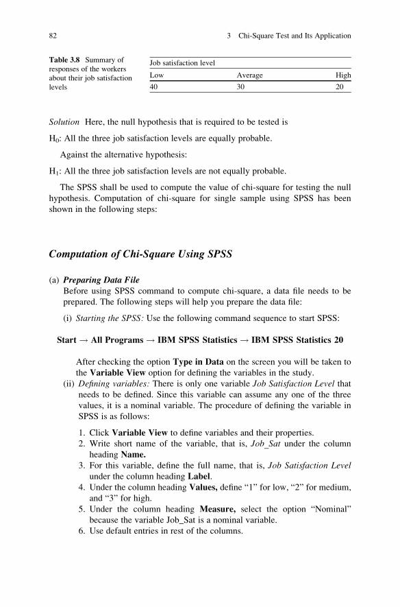
Solution Here, the null hypothesis that is required to be tested is
H0: All the three job satisfaction levels are equally probable.
Against the alternative hypothesis:
H1: All the three job satisfaction levels are not equally probable.
The SPSS shall be used to compute the value of chi-square for testing the null
hypothesis. Computation of chi-square for single sample using SPSS has been
shown in the following steps:
Computation of Chi-Square Using SPSS
(a) Preparing Data FileBefore using SPSS command to compute chi-square, a data file needs to be
prepared. The following steps will help you prepare the data file:
(i) Starting the SPSS: Use the following command sequence to start SPSS:
Start ! All Programs ! IBM SPSS Statistics ! IBM SPSS Statistics 20
After checking the option Type in Data on the screen you will be taken to
the Variable View option for defining the variables in the study.
(ii) Defining variables: There is only one variable Job Satisfaction Level thatneeds to be defined. Since this variable can assume any one of the three
values, it is a nominal variable. The procedure of defining the variable in
SPSS is as follows:
1. Click Variable View to define variables and their properties.
2. Write short name of the variable, that is, Job_Sat under the column
heading Name.
3. For this variable, define the full name, that is, Job Satisfaction Levelunder the column heading Label.
4. Under the column heading Values, define “1” for low, “2” for medium,
and “3” for high.
5. Under the column heading Measure, select the option “Nominal”
because the variable Job_Sat is a nominal variable.
6. Use default entries in rest of the columns.
Table 3.8 Summary of
responses of the workers
about their job satisfaction
levels
Job satisfaction level
Low Average High
40 30 20
82 3 Chi-Square Test and Its Application

After defining the variables in variable view, the screen shall look like
Fig. 3.2.
(iii) Entering data: Once the variable Job_Sat has been defined in the VariableView, click Data View on the left bottom of the screen to open the format
for entering data column wise.
In this example, we have only one variable Job_Sat with three levels as
Low, Medium, and High. The Low satisfaction level was observed in 40
workers, whereas Medium satisfaction level was observed in 30 workers
and High satisfaction level was observed in 20 workers. Since these levels
have been defined as 1, 2, and 3, the data shall be entered under one
variable Job_Sat as shown below:
Data feeding procedure in SPSS under Data View
S.N. Job_Sat
1 1
2 1
3 1 Type “1” 40 times as Low satisfaction level was observed in 40 workers
. .
. .
. .
40 1
41 2
42 2
. . Type “2” 30 times as Medium satisfaction level was observed in 30 workers
. .
. .
70 2
71 3
72 3
73 3 Type “3” 20 times as Low satisfaction level was observed in 20 workers
. .
. .
. .
90 3
Fig. 3.2 Defining variable along with its characteristics
Solved Examples of Chi-square for Testing an Equal Occurrence Hypothesis 83

After entering data, the screen shall look like Fig. 3.3. Only the partial data
has been shown in the figure as data set is long enough to fit in the window.
Save the data file in the desired location before further processing.
(b) SPSS Commands for Computing Chi-SquareAfter preparing the data file in data view, take the following steps to compute
the chi-square:
(i) Initiating the SPSS commands to compute chi-square for single variable: Indata view, click the following commands in sequence:
Analyze ! Nonparametric Tests ! Legacy Dialogs ! Chi� Square
The screen shall look like Fig. 3.4.
Note: In other versions of SPSS, the command sequence is as follows:
Analyze ! Nonparametric Tests ! Chi-Square
(ii) Selecting variable for computing chi-square: After clicking the “Chi-
Square” option, you will be taken to the next screen for selecting the
variable for which chi-square needs to be computed. Since there is only
one variable Jobs satisfaction level in the example, select it from the left
panel by using the left click of the mouse and bring it to the right panel by
clicking the arrow. The screen shall look like Fig. 3.5.
(iii) Selecting the option for computation: After selecting the variable, option
needs to be defined for the computation of chi-square. Take the following
steps:
– Click the Options in the screen shown in Fig. 3.5. This will take you to
the next screen that is shown in Fig. 3.6.
– Check the option “Descriptive.”
– Use default entries in other options.
– Click Continue. This will take you back to screen shown in Fig. 3.5
– Press OK.
(c) Getting the OutputPressing OK will lead you to the output window. The output panel shall have
two results that are shown in Tables 3.9 and 3.10. These outputs can be selected
by using right click of the mouse which may be copied in the word file.
Interpretation of the Outputs
Table 3.9 shows the observed and expected frequencies of the different levels of job
satisfaction. No cell frequency is less than 5, and, therefore, no correction is
required while computing chi-square.
84 3 Chi-Square Test and Its Application

The value of chi-square (¼6.667) in Table 3.10 is significant at 5% level because
its associated p value is .036 which is less than .05. Thus, the null hypothesis may be
rejected. It may therefore be concluded that all the three job satisfaction levels are
not equally probable.
So long the value of p is less than .05, the value of chi-square is significant at 5%
level, and if the p value becomes more than .05, the chi-square becomes
insignificant.
Fig. 3.3 Screen showing
entered data for the variable
Job_Sat in the data view
Solved Examples of Chi-square for Testing an Equal Occurrence Hypothesis 85
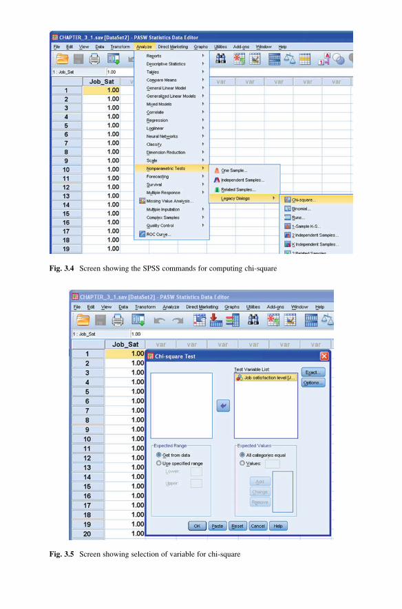
Fig. 3.4 Screen showing the SPSS commands for computing chi-square
Fig. 3.5 Screen showing selection of variable for chi-square

Solved Example of Chi-square for Testing the Significance of
Association Between Two Attributes
Example 3.5 Out of 200 MBA students, 40 were given an academic counseling
throughout the semester, whereas other 40 did not receive this counseling. On the
basis of their marks in the final examination, their performance was categorized as
improved, unchanged, and deteriorated. Based on the results shown in Table 3.11,
can it be concluded that the academic counseling is effective at 5% level?
Fig. 3.6 Screen showing option for chi-square computation
Table 3.9 Observed and
expected frequencies for
different levels of job
satisfaction
Frequencies
Observed N Expected N Residual
Low 40 30.0 10.0
Medium 30 30.0 .0
High 20 30.0 �10.0
Total 90
Table 3.10 Chi-square for
the data on job satisfaction
level
Job satisfaction level
Chi-square 6.667a
df 2
Asymp sig. .036a0 cells (0%) have expected frequencies less than 5. The mini-
mum expected cell frequency is 30
Solved Example of Chi-square for Testing the Significance of Association. . . 87

Solution In order to check whether academic counseling is effective, we shall test the
significance of association between treatment and performance. If the association
between these two attributes is significant, then itmay be interpreted that the pattern of
performance in the counseling and control groups is not same. In that case, it might be
concluded that the counseling is effective since the number of improved cases is
higher in counseling group than that of control group.
Thus, it is important to compute the chi-square first in order to test the null hypothesis.
H0: There is no association between treatment and performance.
Against the alternative hypothesis:
H1: There is an association between treatment and performance.
The commands for computing chi-square in case of two samples are different
than that of one sample computed in Example 3.4.
In two-sample case, chi-square is computed using Crosstabs option in Descrip-
tive statistics command of SPSS. The chi-square so obtained shall be used for
testing the above-mentioned null hypothesis. Computation of chi-square for two
samples using SPSS has been shown in the following steps:
Computation of Chi-Square for Two Variables Using SPSS
(a) Preparing Data FileAs discussed in Example 3.4, a data file needs to be prepared for using the SPSS
commands for computing chi-square. Follow the below-mentioned steps to
prepare data file:
(i) Starting the SPSS: Use the following command sequence to start SPSS:
Start ! All Programs ! IBM SPSS Statistics ! IBM SPSS Statistics 20
By checking the option Type in Data on the screen you will be taken to the
Variable View option for defining the variables in the study.
(ii) Defining variables: Here, two variables Treatment and Performance need
to be defined. Since both these variables are classificatory in nature, they
are treated as nominal variables in SPSS. The procedure of defining
variables and their characteristics in SPSS is as follows:
1. Click Variable View to define variables and their properties.
2. Write short name of the variables as Treatment and Performance underthe column heading Name.
Table 3.11 Frequencies of
the MBA students in a
contingency table Treatment
Performance
Improved Unchanged Deteriorated
Counseling group 22 8 10
Control group 4 5 31
88 3 Chi-Square Test and Its Application
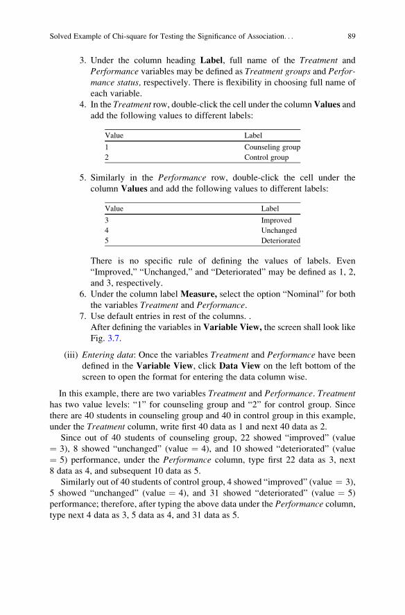
3. Under the column heading Label, full name of the Treatment and
Performance variables may be defined as Treatment groups and Perfor-mance status, respectively. There is flexibility in choosing full name of
each variable.
4. In the Treatment row, double-click the cell under the columnValues and
add the following values to different labels:
Value Label
1 Counseling group
2 Control group
5. Similarly in the Performance row, double-click the cell under the
column Values and add the following values to different labels:
Value Label
3 Improved
4 Unchanged
5 Deteriorated
There is no specific rule of defining the values of labels. Even
“Improved,” “Unchanged,” and “Deteriorated” may be defined as 1, 2,
and 3, respectively.
6. Under the column label Measure, select the option “Nominal” for both
the variables Treatment and Performance.7. Use default entries in rest of the columns. .
After defining the variables in Variable View, the screen shall look like
Fig. 3.7.
(iii) Entering data: Once the variables Treatment and Performance have beendefined in the Variable View, click Data View on the left bottom of the
screen to open the format for entering the data column wise.
In this example, there are two variables Treatment and Performance. Treatmenthas two value levels: “1” for counseling group and “2” for control group. Since
there are 40 students in counseling group and 40 in control group in this example,
under the Treatment column, write first 40 data as 1 and next 40 data as 2.
Since out of 40 students of counseling group, 22 showed “improved” (value
¼ 3), 8 showed “unchanged” (value ¼ 4), and 10 showed “deteriorated” (value
¼ 5) performance, under the Performance column, type first 22 data as 3, next
8 data as 4, and subsequent 10 data as 5.
Similarly out of 40 students of control group, 4 showed “improved” (value ¼ 3),
5 showed “unchanged” (value ¼ 4), and 31 showed “deteriorated” (value ¼ 5)
performance; therefore, after typing the above data under the Performance column,
type next 4 data as 3, 5 data as 4, and 31 data as 5.
Solved Example of Chi-square for Testing the Significance of Association. . . 89

Fig. 3.7 Defining variables along with their characteristics
Data feeding procedure for the data of Table 3.11 in SPSS under Data View
S.N. Treatment Performance
1 1 3
2 1 3
3 1 3 Type “3” twenty-two times as there
are 22 students showed Improved
performance in counseling group4 1 3
5 1 3
6 1 3
7 1 3
8 1 3
9 1 3
10 1 3
11 1 3
12 Type “1” forty
times as there are 40
students in the
counseling group
1 3
13 1 3
14 1 3
15 1 3
16 1 3
17 1 3
18 1 3
19 1 3
20 1 3
21 1 3
22 1 3
23 1 4
24 1 4 Type “4” eight times as there are
8 students showed Unchanged
performance in counseling
group
25 1 4
26 1 4
27 1 4
28 1 4
29 1 4
30 1 4
31 1 5
32 1 5 Type “5” ten times as there are 10
students showed Deteriorated
performance in counseling
group
33 1 5
34 1 5
35 1 5
(continued)
90 3 Chi-Square Test and Its Application
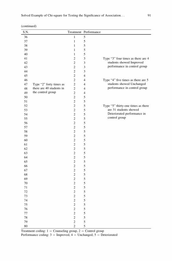
(continued)
S.N. Treatment Performance
36 1 5
37 1 5
38 1 5
39 1 5
40 1 5
41 2 3 Type “3” four times as there are 4
students showed Improved
performance in control group42 2 3
43 2 3
44 2 3
45 2 4
46 2 4 Type “4” five times as there are 5
students showed Unchanged
performance in control group47 Type “2” forty times as
there are 40 students in
the control group
2 4
48 2 4
49 2 4
50 2 5
51 2 5
52 2 5 Type “5” thirty-one times as there
are 31 students showed
Deteriorated performance in
control group
53 2 5
54 2 5
55 2 5
56 2 5
57 2 5
58 2 5
59 2 5
60 2 5
61 2 5
62 2 5
63 2 5
64 2 5
65 2 5
66 2 5
67 2 5
68 2 5
69 2 5
70 2 5
71 2 5
72 2 5
73 2 5
74 2 5
75 2 5
76 2 5
77 2 5
78 2 5
79 2 5
80 2 5
Treatment coding: 1 ¼ Counseling group, 2 ¼ Control group
Performance coding: 3 ¼ Improved, 4 ¼ Unchanged, 5 ¼ Deteriorated
Solved Example of Chi-square for Testing the Significance of Association. . . 91

After entering the data, the screen will look like Fig. 3.8. The screen shows only
the partial data as the data is entered column wise which takes two-page-long
entries. Save the data file in the desired location before further processing.
(b) SPSS Commands for Computing Chi-square with Two VariablesAfter entering all the data by clicking the data view, take the following steps for
computing chi-square:
(i) Initiating the SPSS commands for computing chi-square: In Data View,
click the following commands in sequence:
Analyze ! Descriptive Statistics ! Crosstabs
The screen shall look like Fig. 3.9.
(ii) Selecting variables for computing chi-square: After clicking the
“Crosstabs” option, you will be taken to the next screen for selecting
variables for the crosstabs analysis and computing chi-square. Out of the
two variables, one has to be selected in the Row(s) panel and the other in
the Column(s) panel.
Fig. 3.8 Screen showing
entered data for the Treatmentand Performance variables inthe data view
92 3 Chi-Square Test and Its Application

Select the variables Treatment group and Performance status from the left
panel and bring them to the “Row(s)” and “Column(s)” sections of the right
panel, respectively, by arrow button. The screen shall look like Fig. 3.10.
(iii) Selecting option for computation: After selecting variables, option needs
to be defined for the crosstabs analysis and computation of chi-square.
Take the following steps:
– Click Statistics option to get the screen shown in Fig. 3.11.
– Check the options “Chi-square” and “Contingency coefficient.”
– Click Continue.
– Click Cells option to get the screen shown in Fig. 3.12. Then,
– Check the options “Observed” and “Expected” under the Counts
section. Observed is checked by default.
– Click Continue. You will be taken back to the screen shown in
Fig. 3.10.
– Use default entries in other options. Readers are advised to try other
options and see what changes they are getting.
– Click OK.
Fig. 3.9 Screen showing the SPSS commands for computing chi-square in crosstabs
Solved Example of Chi-square for Testing the Significance of Association. . . 93

Figure 3.10 Screen showing selection of variables for chi-square in crosstab
Fig. 3.11 Screen showing option for computing chi-square and contingency coefficient
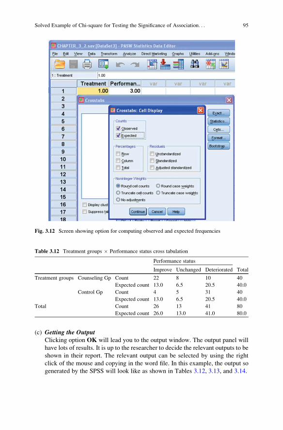
(c) Getting the OutputClicking option OK will lead you to the output window. The output panel will
have lots of results. It is up to the researcher to decide the relevant outputs to be
shown in their report. The relevant output can be selected by using the right
click of the mouse and copying in the word file. In this example, the output so
generated by the SPSS will look like as shown in Tables 3.12, 3.13, and 3.14.
Fig. 3.12 Screen showing option for computing observed and expected frequencies
Table 3.12 Treatment groups � Performance status cross tabulation
Performance status
TotalImprove Unchanged Deteriorated
Treatment groups Counseling Gp Count 22 8 10 40
Expected count 13.0 6.5 20.5 40.0
Control Gp Count 4 5 31 40
Expected count 13.0 6.5 20.5 40.0
Total Count 26 13 41 80
Expected count 26.0 13.0 41.0 80.0
Solved Example of Chi-square for Testing the Significance of Association. . . 95

Interpretation of the Outputs
The observed and expected frequencies of the Treatment group � Performancestatus can be seen in Table 3.12. Since no cell frequency is less than 5, therefore, nocorrection is required while computing the chi-square. If any of the cell frequency
had value 5 or less, then SPSS would have computed the chi-square after applying
the correction.
Table 3.13 shows the value of chi-square (w2) as 23.910, which is significant at 1%level as the p value is .000. Thus, we may reject the null hypothesis that “There is no
association between Treatment and Performance.” Hence, it may be concluded that
there is a significant association between treatment and performance. In other words,
it can be said that the pattern of academic performance is different in counseling and
control group. Since the number of improved performance cases (22) is higher in
counseling group than that of 4 in control group, it may be interpreted that the
academic counseling is effective in improving the performance.
In Table 3.14, the value of contingency coefficient is 0.480. This is a measure of
association between Treatment and Performance. This contingency coefficient can
be considered to be significant as its p value is .000 which is less than .05. Thus, it
may finally be concluded that counseling is significantly effective in improving the
academic performance.
Summary of the SPSS Commands
(a) For computing chi-square statistic (for testing equal occurrence
hypothesis):
1. Start SPSS by using the following sequence of commands:
Start ! All Programs ! IBM SPSS Statistics ! IBM SPSS Statistics 20
Table 3.14 Contingency coefficient for the data on Treatment � Performance
Value Approx. sig. (p value)
Nominal by nominal Contingency coefficient 0.480 0.000
N of valid cases 80
Table 3.13 Chi-square for the data on Treatment � Performance
Value df Asymp. sig. (2-sided)
Pearson chi-square 23.910a 2 .000
Likelihood ratio 25.702 2 .000
Linear-by-linear association 23.400 1 .000
N of valid cases 80a0 cells (.0%) have expected count less than 5. The minimum expected count is 6.50
96 3 Chi-Square Test and Its Application

2. Create data file by choosing the option Type in Data.
3. Click the tag Variable View and define the variable Job_Sat as “Nominal”
variable.
4. For the variable Job_Sat, under the column heading Values, define “1” for
low, “2” for medium, and “3” for high.
5. By clicking the Data View, enter first forty data of the variable Job_Sat as 1,next thirty as 2, and further 20 as 3 in the same column.
6. Click the following command sequence for computing chi-square:
Analyze ! Nonparametric Tests ! Legacy Dialogs ! Chi� Square
7. Select the variable Job_Sat from left panel to the right panel.
8. Click the tag Options and check the box of “Descriptive.” Press Continue.9. Click OK to get the output.
(b) For computing chi-square statistic (for testing the significance of associa-
tion between two attributes):
1. Start SPSS by using the following command sequence:
Start ! All Programs ! IBM SPSS Statistics ! IBM SPSS Statistics 20
2. Click Variable View tag and define the variable Treatment and Perfor-mance as “Nominal” variables.
3. In the Treatment row, double-click the cell under the column Values and
add the values “1” for Counseling group and “2” for Control group.
Similarly, in the Performance row, define the value “3” for Improved,
4 for Unchanged, and 5 for Deteriorated.
4. Use default entries in rest of the columns.
5. Click Data View tag and feed first forty entries as 1 and next forty entries
as 2 for the Treatment variable.6. Similarly for the Performance variable, enter first twenty-two entries as 3,
next eight entries as 4, and further ten entries as 5. These three sets of
entries are for counseling group. Similarly for showing the entries of
control group, enter first four entries as 3, next five entries as 4, and after
that thirty-one entries as 5 in the same column.
7. Click the following command sequence for computing chi-square:
Analyze ! Descriptive Statistics ! Crosstabs
8. Select variables Treatment group and Performance status from the left panel
to the “Row(s)” and “Column(s)” sections of the right panel, respectively.
9. Click the option Statistics and check the options “Chi-square” and “Con-
tingency coefficient.” Press Continue.10. Click OK to get the output.
Summary of the SPSS Commands 97

Exercise
Short-Answer Questions
Note: Write answer to each of the questions in not more than 200 words:
Q.1. Responses were obtained from male and female on different questions related
to their knowledge about smoking. There were three possible responses
Agree, Undecided, and Disagree for each of the questions. How will you
compare the knowledge of male and female about smoking?
Q.2. Write in brief two important applications of chi-square.
Q.3. How will you frame a null hypothesis in testing the significance of an associ-
ation between gender and IQ where IQ is classified into high and low
category? Write the decision criteria in testing the hypothesis.
Q.4. Can the chi-square be used for comparing the attitude of male and female on
the issue of “Foreign retail chain may be allowed in India” if the frequencies
are given in 3 � 5 table below? If so or otherwise, interpret your findings.
Under what situation chi-square is the most robust test?
Q.5 If chi-square is significant, it indicates that the association between the two
attributes exists. How would you find the magnitude of an association?
Q.6 What is phi coefficient? In what situation it is used? Explain by means of an
example.
Multiple-Choice Questions
Note: For each of the question, there are four alternative answers. Tick mark the
one that you consider the closest to the correct answer.
1. For testing the significance of association between Gender and IQ level, the
command sequence for computing chi-square in SPSS is
(a) Analyze -> Nonparametric Tests -> Chi-square
(b) Analyze -> Descriptive Statistics -> Crosstabs
(c) Analyze -> Chi-square -> Nonparametric Tests
(d) Analyze -> Crosstabs -> Chi-square
2. Choose the most appropriate statement about the null hypothesis in chi-square.
(a) There is an association between gender and response.
(b) There is no association between gender and response.
(c) There are 50�50% chances of significant and insignificant association.
(d) None of the above is correct.
Response on “Foreign retail chain may be allowed in India”
Strongly agree Agree Undecided Disagree Strongly disagree
Gender Male 50 20 15 5 10
Female 20 15 10 25 30
98 3 Chi-Square Test and Its Application
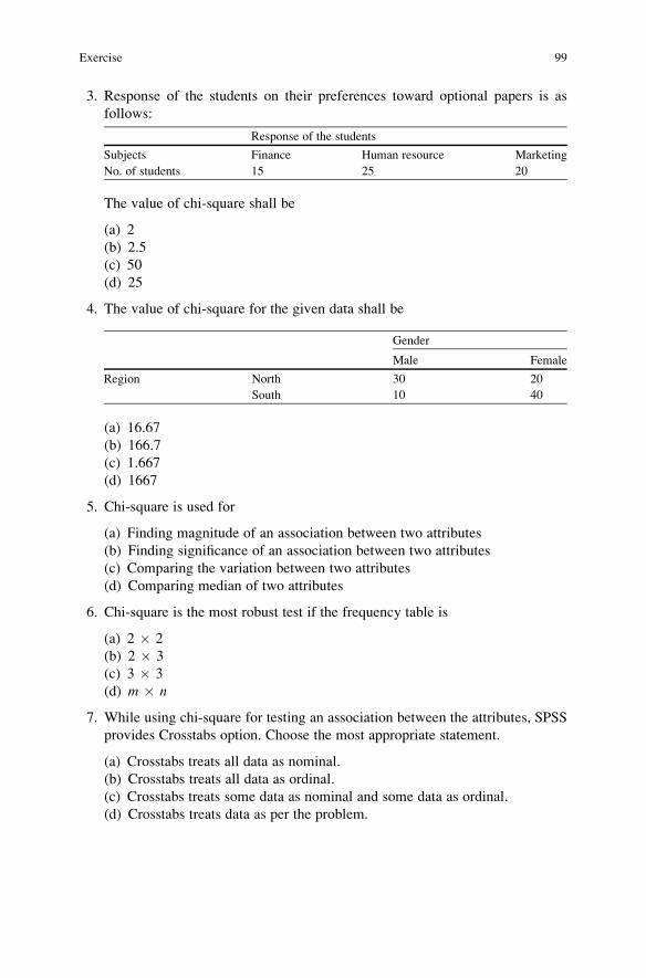
3. Response of the students on their preferences toward optional papers is as
follows:
Response of the students
Subjects Finance Human resource Marketing
No. of students 15 25 20
The value of chi-square shall be
(a) 2
(b) 2.5
(c) 50
(d) 25
4. The value of chi-square for the given data shall be
Gender
Male Female
Region North 30 20
South 10 40
(a) 16.67
(b) 166.7
(c) 1.667
(d) 1667
5. Chi-square is used for
(a) Finding magnitude of an association between two attributes
(b) Finding significance of an association between two attributes
(c) Comparing the variation between two attributes
(d) Comparing median of two attributes
6. Chi-square is the most robust test if the frequency table is
(a) 2 � 2
(b) 2 � 3
(c) 3 � 3
(d) m � n
7. While using chi-square for testing an association between the attributes, SPSS
provides Crosstabs option. Choose the most appropriate statement.
(a) Crosstabs treats all data as nominal.
(b) Crosstabs treats all data as ordinal.
(c) Crosstabs treats some data as nominal and some data as ordinal.
(d) Crosstabs treats data as per the problem.
Exercise 99

8. If responses are obtained in the form of the frequency on a 5-point scale and it is
required to compare the responses of male and female on the issue “Marketing
stream is good for the female students,” which statistical test you would prefer?
(a) Two-sample t-test(b) Paired t-test(c) One-way ANOVA
(d) Chi-square test
9. If p value for a chi-square is .02, what conclusion you can draw?
(a) Chi-square is significant at 95% confidence.
(b) Chi-square is not significant at 95% confidence.
(c) Chi-square is significant at .01 levels.
(d) Chi-square is not significant at .05 levels.
10. The degree of freedom of chi-square in a r � c table is
(a) r + c(b) r + c�1
(c) rc(d) (r�1)(c�1)
11. Phi coefficient is used if
(a) Both the variables are ordinal.
(b) Both the variables are binary.
(c) Both the variables are interval.
(d) One of the variables is nominal and the other is ordinal.
12. Gamma coefficient is used if
(a) Both the variables are interval.
(b) Both the variables are binary.
(c) Both the variables are ordinal.
(d) Both the variables may be on any scale.
Assignments
1. Following are the frequencies of students in an institute belonging to Low,
Medium, and High IQ groups. Can it be concluded that there is a specific
trend of IQ’s among the students. Test your hypothesis at 5% level.
Frequencies of the students in different IQ groups
IQ categories Low IQ Medium IQ High IQ
Frequency 20 65 35
2. In an organization following are the frequencies of male and female workers in
the skilled and unskilled categories. Test whether nature of work is independent
of the gender by computing chi-square. Also compute contingency coefficient
100 3 Chi-Square Test and Its Application

along with the expected frequency and percentage frequencies in the Crosstabs
and interpret your findings. Test your hypothesis at 5% level.
Frequency of workers in different categories
Workers
Skilled Unskilled
Gender Male 50 15
Female 15 40
Answers to Multiple-Choice Questions
Q.1 b Q.2 b
Q.3 b Q.4 a
Q.5 b Q.6 a
Q.7 a Q.8 d
Q.9 a Q.10 d
Q.11 b Q.12 c
Exercise 101

Chapter 4
Correlation Matrix and Partial Correlation:
Explaining Relationships
Learning Objectives
After completing this chapter, you should be able to do the following:
• Learn the concept of linear correlation and partial correlation.
• Explore the research situations in which partial correlation can be effectively
used.
• Understand the procedure in testing the significance of product moment correla-
tion and partial correlation.
• Develop the hypothesis to test the significance of correlation coefficient.
• Formulate research problems where correlation matrix and partial correlation
can be used to draw effective conclusion.
• Learn the application of correlation matrix and partial correlation through case
study discussed in this chapter.
• Understand the procedure of using SPSS in computing correlation matrix and
partial correlation.
• Interpret the output of correlation matrix and partial correlation generated in
SPSS.
Introduction
One of the thrust areas in the management research is to find the ways and means to
improve productivity. It is therefore important to know the variables that affect it.
Once these variables are identified, an effective strategy may be adopted by
prioritizing it to enhance the productivity in the organization. For instance, if a
company needs to improve the sale of a product, then its first priority would be to
ensure its quality and then to improve other variables like resources available to the
marketing team, their incentive criteria, and dealer’s scheme. It is because of the
fact that the product quality is the most important parameter in enhancing sale.
J.P. Verma, Data Analysis in Management with SPSS Software,DOI 10.1007/978-81-322-0786-3_4, # Springer India 2013
103

To find how strongly a given variable is associated with the performance of an
employee, an index known as product moment correlation coefficient “r” may be
computed. The product moment correlation coefficient is also known as correlation
coefficient, and it measures only linear relation between two variables.
When we have two variables that covary, there are two possibilities. First, the
change in a thing is concomitant with the change in another, as the change in a
child’s age covaries with his weight, that is, the older, the heavier. When higher
magnitude on one variable occurs along with higher magnitude on another and the
lower magnitudes on both also occur simultaneously, then the things vary together
positively, and we denote this situation as positive correlation.
In the second situation, two things vary inversely. In other words, the higher
magnitudes of one variable go along with the lower magnitudes of the other and
vice versa. This situation is denoted as negative correlation.
The higher magnitude of correlation coefficient simply indicates that there is
more likelihood that if the value of one variable increases, the value of other
variable also increases or decreases. However, correlation coefficient does not
reveal the real relationship between the two variables until the effects of other
variables are eliminated.
This fact can be well explained with the following example. John and Philip
work for the same company. John has a big villa costing $540,000, whereas Philip
owns a three-room apartment, costing $160,000. Which person has a greater salary?
Here, one can reasonably assume that it must be John who earns more, as he has
a more expensive house. As he earns a larger salary, the chances are that he can
afford a more expensive house. One cannot be absolutely certain; of course, it may
be that John’s villa was a gift from his father, or he could have gotten it in a contest
or it might be a result of any legal settlement. However, most of the time, an
expensive house means a larger salary.
In this case, one may conclude that there is a correlation between someone’s
salary and the cost of the house that he/she possesses. This means that as one figure
changes, one can expect the other to change in a fairly regular way.
In order to be confident that the relationship exists between any two variables, it
must be exhibited across some cases. A case is a component of variation in a thing.
For example, different levels of IQ that go along with different marks obtained in
the final examination may be perceived across students. If the correlation between
IQ and marks of the students is positive, it indicates that a student with high IQ has
high marks and the one with low IQ has low marks.
The correlation coefficient gives fair estimate of the extent of relationship
between any two variables if the subjects are chosen at random. But in most of
the situations, samples are purposive, and, therefore, correlation coefficient in
general may not give the correct picture of the real relationship. For example, in
finding correlation coefficient between the age of customers and quantity of mois-
turizer purchased, if the sample is collected from the high socioeconomic popula-
tion, the result may not be valid as in this section of society, people understand the
importance of the product and can afford to invest on it. However, to establish the
relationship between sales and age of the users, one should collect the sample from
all the socioeconomic status groups.
104 4 Correlation Matrix and Partial Correlation: Explaining Relationships
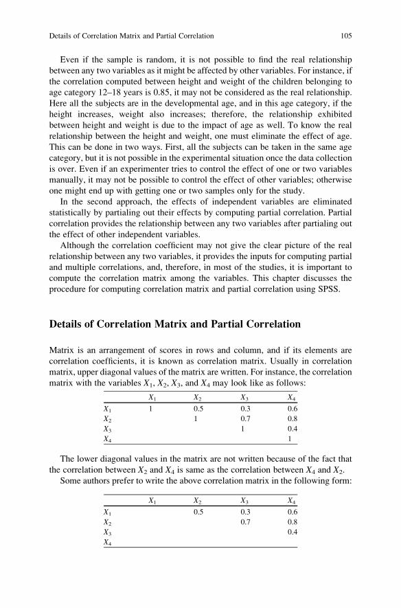
Even if the sample is random, it is not possible to find the real relationship
between any two variables as it might be affected by other variables. For instance, if
the correlation computed between height and weight of the children belonging to
age category 12–18 years is 0.85, it may not be considered as the real relationship.
Here all the subjects are in the developmental age, and in this age category, if the
height increases, weight also increases; therefore, the relationship exhibited
between height and weight is due to the impact of age as well. To know the real
relationship between the height and weight, one must eliminate the effect of age.
This can be done in two ways. First, all the subjects can be taken in the same age
category, but it is not possible in the experimental situation once the data collection
is over. Even if an experimenter tries to control the effect of one or two variables
manually, it may not be possible to control the effect of other variables; otherwise
one might end up with getting one or two samples only for the study.
In the second approach, the effects of independent variables are eliminated
statistically by partialing out their effects by computing partial correlation. Partial
correlation provides the relationship between any two variables after partialing out
the effect of other independent variables.
Although the correlation coefficient may not give the clear picture of the real
relationship between any two variables, it provides the inputs for computing partial
and multiple correlations, and, therefore, in most of the studies, it is important to
compute the correlation matrix among the variables. This chapter discusses the
procedure for computing correlation matrix and partial correlation using SPSS.
Details of Correlation Matrix and Partial Correlation
Matrix is an arrangement of scores in rows and column, and if its elements are
correlation coefficients, it is known as correlation matrix. Usually in correlation
matrix, upper diagonal values of the matrix are written. For instance, the correlation
matrix with the variables X1, X2, X3, and X4 may look like as follows:
X1 X2 X3 X4
X1 1 0.5 0.3 0.6
X2 1 0.7 0.8
X3 1 0.4
X4 1
The lower diagonal values in the matrix are not written because of the fact that
the correlation between X2 and X4 is same as the correlation between X4 and X2.
Some authors prefer to write the above correlation matrix in the following form:
X1 X2 X3 X4
X1 0.5 0.3 0.6
X2 0.7 0.8
X3 0.4
X4
Details of Correlation Matrix and Partial Correlation 105

In this correlation matrix, diagonal values are not written as it is obvious that these
values are 1 because correlation between the same two variables is always one.
In this section, we shall discuss the product moment correlation and partial
correlation along with testing of their significance.
Product Moment Correlation Coefficient
Product moment correlation coefficient is an index which provides the magnitude
of linear relationship between any two variables. When we refer to correlation
matrix, it is usually a matrix of product moment correlation coefficients. It is
represented by “r” and is given by the following formula:
r ¼ NSXY � ðSXÞðSYÞffiffiffiffiffiffiffiffiffiffiffiffiffiffiffiffiffiffiffiffiffiffiffiffiffiffiffiffiffiffiffiffiffiffiffiffiffiffiffiffiffiffiffiffiffiffiffiffiffiffiffiffiffiffiffiffiffiffiffiffiffiffiffiffi½NSX2 � ðSXÞ2�½NSY2 � ðSYÞ2�
q (4.1)
where N is the number of paired scores. The limits of r are from �1 to +1. The
positive value of rmeans higher scores on one variable tend to be paired with higher
scores on the other, or lower scores on one variable tend to be paired with lower
scores on the other. On the other hand, negative value of r means higher scores on
one variable tend to be paired with lower scores on the other and vice versa. Further,
r ¼ +1 indicates the perfect positive relationship between the two variables. This
means that if there is an increase (decrease) in X by an amount “a,” the Ywill also be
increased (decreased) by the same amount. Similarly r ¼ �1 signifies the perfect
negative linear correlation between the two variables. In this case, if the variable Xis increased (decreased) by an amount “b,” then the variable Y shall be decreased
(increased) by the same amount. The three extreme values of the correlation
coefficient r can be shown graphically in Fig. 4.1.
Example 4.1: Following are the scores on age and memory retention. Compute the
correlation coefficient and test its significance at 5% level (Table 4.1).
Solution In order to compute the correlation coefficient, first of all the summationPX,P
Y,P
X2,P
Y2, and
PXY shall be computed in Table 4.2.
Fig. 4.1 Graphical presentations of the three extreme cases of correlation coefficient
106 4 Correlation Matrix and Partial Correlation: Explaining Relationships

Here N is 10:
r ¼ NSXY � ðSXÞðSYÞffiffiffiffiffiffiffiffiffiffiffiffiffiffiffiffiffiffiffiffiffiffiffiffiffiffiffiffiffiffiffiffiffiffiffiffiffiffiffiffiffiffiffiffiffiffiffiffiffiffiffiffiffiffiffiffiffiffiffiffiffiffiffiffi½NSX2 � ðSXÞ2�½NSY2 � ðSYÞ2�
qSubstituting the values in the equation,
r ¼ 10� 597� 91� 67ffiffiffiffiffiffiffiffiffiffiffiffiffiffiffiffiffiffiffiffiffiffiffiffiffiffiffiffiffiffiffiffiffiffiffiffiffiffiffiffiffiffiffiffiffiffiffiffiffiffiffiffiffiffiffiffiffiffiffiffiffiffiffiffiffiffi½10� 853� 912�½10� 461� 672�
q¼ �127ffiffiffiffiffiffiffiffiffiffiffiffiffiffiffiffiffiffiffiffiffi
249� 121p ¼ �0:732
Testing the Significance
To test whether the correlation coefficient�0.732 is significant or not, the tabulated
value of r required for significance at .05 level of significance and N � 2(¼8)
degree of freedom can be seen from Table A.3 in the Appendix, which is 0.632.
Hence, it may be concluded that there is a significant negative relationship between
age and memory retention power. In other words, it may be inferred that as the age
increases, the memory retention power decreases.
Table 4.1 Data on age and
memory retentionS.N. Age Memory retention
1 11 7
2 12 5
3 8 7
4 9 6
5 7 8
6 10 5
7 8 7
8 9 8
9 10 6
10 7 8
Table 4.2 Computation for
correlation coefficientAge Memory retention
S.N. (X) (Y) X2 Y2 XY
1 11 7 121 49 77
2 12 5 144 25 60
3 8 7 64 49 56
4 9 6 81 36 54
5 7 8 49 64 56
6 10 5 100 25 50
7 8 7 64 49 56
8 9 8 81 64 72
9 10 6 100 36 60
10 7 8 49 64 56
Total 91 67 853 461 597
Details of Correlation Matrix and Partial Correlation 107
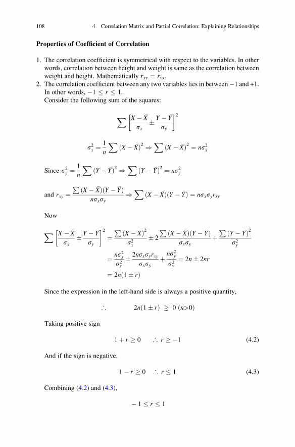
Properties of Coefficient of Correlation
1. The correlation coefficient is symmetrical with respect to the variables. In other
words, correlation between height and weight is same as the correlation between
weight and height. Mathematically rxy ¼ ryx.2. The correlation coefficient between any two variables lies in between�1 and +1.
In other words, �1 � r � 1.
Consider the following sum of the squares:
X X � �X
sx� Y � �Y
sy
� �2
s2x ¼1
n
XX � �Xð Þ2 )
XX � �Xð Þ2 ¼ ns2x
Since s2y ¼1
n
XY � �Yð Þ2 )
XY � �Yð Þ2 ¼ ns2y
and rxy ¼P ðX � �XÞðY � �YÞ
nsxsy)X
ðX � �XÞðY � �YÞ ¼ nsxsyrxy
Now
X X � �X
sx� Y � �Y
sy
� �2¼P
X � �Xð Þ2s2x
� 2
PX � �Xð Þ Y � �Yð Þ
sxsyþP
Y � �Yð Þ2s2y
¼ ns2xs2x
� 2nsxsyrxysxsy
þ ns2ys2y
¼ 2n� 2nr
¼ 2nð1� rÞ
Since the expression in the left-hand side is always a positive quantity,
; 2n 1� rð Þ � 0 n>0ð Þ
Taking positive sign
1þ r � 0 ; r � �1 (4.2)
And if the sign is negative,
1� r � 0 ; r � 1 (4.3)
Combining (4.2) and (4.3),
� 1 � r � 1
108 4 Correlation Matrix and Partial Correlation: Explaining Relationships
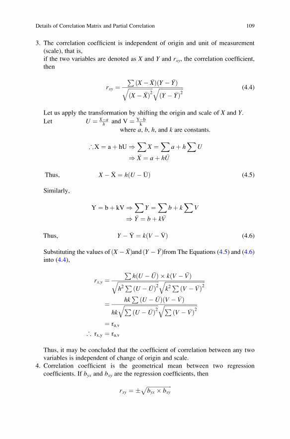
3. The correlation coefficient is independent of origin and unit of measurement
(scale), that is,
if the two variables are denoted as X and Y and rxy, the correlation coefficient,
then
rxy ¼P
X � �Xð Þ Y � �Yð ÞffiffiffiffiffiffiffiffiffiffiffiffiffiffiffiffiffiffiX � �Xð Þ2
q ffiffiffiffiffiffiffiffiffiffiffiffiffiffiffiffiffiffiY � �Yð Þ2
q (4.4)
Let us apply the transformation by shifting the origin and scale of X and Y.
Let U ¼ X�ah and V ¼ Y�b
k
where a, b, h, and k are constants.
;X ¼ aþ hU )X
X ¼X
aþ hX
U
) �X ¼ aþ h �U
Thus, X � �X ¼ hðU � �UÞ (4.5)
Similarly,
Y ¼ bþ kV )X
Y ¼X
bþ kX
V
) �Y ¼ bþ k �V
Thus, Y � �Y ¼ kðV � �VÞ (4.6)
Substituting the values of ðX � �XÞand ðY � �YÞfrom The Equations (4.5) and (4.6)
into (4.4),
rx;y ¼P
hðU � �UÞ � kðV � �VÞffiffiffiffiffiffiffiffiffiffiffiffiffiffiffiffiffiffiffiffiffiffiffiffiffiffiffiffiffiffih2P
U � �Uð Þ2q ffiffiffiffiffiffiffiffiffiffiffiffiffiffiffiffiffiffiffiffiffiffiffiffiffiffiffiffiffi
k2P
V � �Vð Þ2q
¼ hkP ðU � �UÞðV � �VÞ
hk
ffiffiffiffiffiffiffiffiffiffiffiffiffiffiffiffiffiffiffiffiffiffiffiffiffiPU � �Uð Þ2
q ffiffiffiffiffiffiffiffiffiffiffiffiffiffiffiffiffiffiffiffiffiffiffiffiPV � �Vð Þ2
q¼ ru;v
; rx;y ¼ ru;v
Thus, it may be concluded that the coefficient of correlation between any two
variables is independent of change of origin and scale.
4. Correlation coefficient is the geometrical mean between two regression
coefficients. If byx and bxy are the regression coefficients, then
rxy ¼ � ffiffiffiffiffiffiffiffiffiffiffiffiffiffiffiffiffiffibyx � bxy
p
Details of Correlation Matrix and Partial Correlation 109

Correlation Coefficient May Be Misleading
As per the definition, correlation coefficient indicates the linear relationship
between the two variables. This value may be misleading at times. Look at the
following three situations:
1. Researchers often conclude that a high degree of correlation implies a causal
relationship between the two variables, but this is totally unjustified. For example,
both events, represented by X1 and X2, might simply have a common cause. If in a
study, X1 represents the gross salary of the family per month and X2 is the amount
of money spent on the sports and leisure activities per month, then a strong
positive correlation between X1 and X2 should not be concluded that the people
spend more on sports and leisure activities if their family income is more. Now, if
a third variable X3, the socioeconomic status, is taken into account, it becomes
clear that, despite the strong positive value of their correlation coefficient, there is
no causal relationship between “sports and leisure expenditure” and “family
income,” and that both are in fact caused by the third variable “socioeconomic
status.” It is not the family income which encourages a person to spend more on
sports and leisure activities but the socioeconomic status which is responsible for
such a behavior. To know the causal relationship, partial correlation may be used
with limitations.
2. A low or insignificant value of the correlation coefficient may not signify the lack
of a strong link between the two variables under consideration. The lower value of
correlation coefficient may be because of the other variables affecting the
relationships in a negative manner. And, therefore, the effect of those variables
eliminated may increase the magnitude of the correlation coefficient. Path Analy-
sis may provide the insight in this direction where a correlation coefficient may be
split into direct and indirect relationships.
3. The ecological fallacy is another source of misleading correlation coefficient. It
occurs when a researcher makes an inference about the correlation in a particular
situation based on correlation of aggregate data for a group. For instance, if a
high degree of relationship exists between height and performance of athletes in
the USA, it does not indicate that every tall athlete’s performance is excellent in
the USA. And if we conclude so, it will be an ecological fallacy.
4. Correlation does not explain causative relationship. High degree of correlation
between two variables does not indicate that one variable causes another. In other
words, correlation does not show cause and effect relationship. In a distance
learning program, if there is a high degree of correlation between the student’s
performance and the number of contact classes attended, it does not necessarily
indicate that one gets more marks because he learns more during contact classes.
Neither does it necessarily imply that the more classes you attend, the more
intelligent you become and get good marks. Some other explanation might also
explain the correlation coefficient. The correlation means that the one who attends
more contact classes gets higher marks and those who attend less classes get less
marks. It does not explain why it is the case.
110 4 Correlation Matrix and Partial Correlation: Explaining Relationships
5. One must ensure that the result of correlation coefficient should be generalized
only for that population from which the sample was drawn. Usually for a specific
small sample, correlation may be high for any two variables, and if it is so, then it
must be verified with the larger representative and relevant sample.
Limitations of Correlation Coefficients
One of the main limitations of the correlation coefficient is that it measures only
linear relationship between the two variables. Thus, correlation coefficient should
be computed only when the data are measured either on interval scale or ratio scale.
The other limitation of the correlation coefficient is that it does not give the real
relationship between the variables. To overcome this problem, partial correlation
may be computed which explains the real relationship between the variables after
controlling for other variables with certain limitations.
Testing the Significance of Correlation Coefficient
After computing the correlation coefficient, the next question is to find as to
whether it actually explains some relationship or it is due to chance.
The following mutually exclusive hypotheses are tested by using the statistical
test for testing the significance of correlation coefficient:
H0: �r ¼ 0 (There is no correlation between the two variables in the population.)
H1: �r 6¼ 0 (There is a correlation between the two variables in the population.)
In fact, �r indicates the population correlation coefficient, and we test its signifi-
cance on the basis of the sample correlation coefficient. To test the above set of
hypotheses, any of the following three approaches may be used.
First Approach
The easiest way to test the null hypothesis mentioned above is to look for the critical
value of r with n � 2 degrees of freedom at any desired level of significance in
Table A.3 in the Appendix. If the calculated value of r is less than or equal to the
critical value of r, null hypothesis would fail to be rejected, and if calculated r isgreater than critical value of r, null hypothesis may be rejected. For instance, if the
correlation coefficient between height and self-esteem of 25 individuals is 0.45,
then the critical value of r required for significance at .05 level of significance and
N � 2(¼23) df from Table A.3 in the Appendix can be seen as 0.396. Since
calculated value of r, that is, 0.45 is greater than the critical value of r (¼0.396),
the null hypothesis may be rejected at .05 level of significance, and we may
conclude that there is a significant correlation between height and self-esteem.
Details of Correlation Matrix and Partial Correlation 111

Second Approach
Significance of correlation coefficient may be tested by using t-test as well. In this
case, t-statistic is given by the following formula:
t ¼ rffiffiffiffiffiffiffiffiffiffiffiffiffi1� r2
p ffiffiffiffiffiffiffiffiffiffiffin� 2
p(4.7)
Here r is the observed correlation coefficient and n is the number of paired sets of
data.
The calculated value of t is compared with that of tabulated value of t at .05 leveland n�2 df (¼t.05(n�2)). The value of tabulated t can be obtained from Table A.2 in
the Appendix.
Thus, if Cal t � t.05(n�2), null hypothesis is failed to be rejected at .05 level of significance
and if Cal t > t.05(n�2), null hypothesis may be rejected at .05 level of significance
Third Approach
In this approach, significance of correlation coefficient is tested on the basis of its
p value. p value is the probability of wrongly rejecting the null hypothesis. If
p value is .04 for a given correlation coefficient, it indicates that the chances of
wrongly rejecting the null hypothesis are only 4%. Thus, so long p value is less than.05 the correlation coefficient is significant and the null hypothesis may be rejected
at 5% level. On the other hand, if p value is more than or equal to .05, the correlation
coefficient is not significant and the null hypothesis may not be rejected at 5% level.
Note: The SPSS output follows third approach and provides p values for each of thecorrelation coefficient in the correlation matrix.
Partial Correlation
Partial correlation is the measure of relationship between two variables after
partialing out the effect of one or more independent variables. In computing partial
correlation, the data must be measured either on interval or on ratio scale. For
example, one may compute partial correlation if it is desired to see the relationship
of age with stock portfolio after controlling the effect of income. Similarly to
understand the relationship between price and demand would involve studying
the relationship between price and demand after controlling the effect of money
supply, exports, etc.
The partial correlation between X1 and X2 adjusted for X3 is given by
112 4 Correlation Matrix and Partial Correlation: Explaining Relationships

r12:3 ¼ r12 � r13r23ffiffiffiffiffiffiffiffiffiffiffiffiffiffiffiffiffiffiffiffiffiffiffiffiffiffiffiffiffiffiffiffiffiffiffið1� r213Þð1� r223Þ
p (4.8)
The limits of partial correlation are �1 to +1.
The order of partial correlation refers to the number of independent variables
whose effects are to be controlled. Thus, first-order partial correlation controls the
effect of one variable, second-order partial correlation controls the effect of two
variables, and so on.
The generalized formula for (n � 2)th order partial correlation is given by
r12:34:::::::n ¼r12:345::::ðn�1Þ � r1n:345...ðn�1Þr2n:345::::ðn�1Þffiffiffiffiffiffiffiffiffiffiffiffiffiffiffiffiffiffiffiffiffiffiffiffiffiffiffiffiffiffiffiffi
1� r21n:345::::ðn�1Þ
q ffiffiffiffiffiffiffiffiffiffiffiffiffiffiffiffiffiffiffiffiffiffiffiffiffiffiffiffiffiffiffiffi1� r2
2n:345::::ðn�1Þq (4.9)
Limitations of Partial Correlation
1. Since partial correlation is computed by using product moment correlation
coefficient, it also assumes the linear relationship. But generally, this assumption
is not valid especially in social sciences, as linear relationship rarely exists in
such parameters.
2. The reliability of partial correlation decreases if its order increases.
3. Large number of data is required to draw the valid conclusions from the partial
correlations.
4. In spite of controlling the effect of many variables, one cannot be sure that the
partial correlation explains the real relationship.
Testing the Significance of Partial Correlation
The significance of partial correlation is tested in a similar way as has been
discussed above in case of product moment correlation.
In SPSS, significance of partial correlation is tested on the basis of p value. The
partial correlation would be significant at 5% level if its p value is less than .05 andwill be insignificant if the p value is equal to or more than .05.
Computation of Partial Correlation
Example 4.2: The following correlation matrix shows the correlation among
different academic performance parameters. Compute partial correlations r12.3and r12.34 and test their significance. Interpret the findings also (Table 4.3).
Details of Correlation Matrix and Partial Correlation 113

Solution
(i) Computation of r12:3
Since we know that r12:3 ¼ r12 � r13r23ffiffiffiffiffiffiffiffiffiffiffiffiffiffi1� r213
q ffiffiffiffiffiffiffiffiffiffiffiffiffiffi1� r223
qSubstituting the values of correlation coefficients from the correlation matrix,
we get
r12:3 ¼ 0:7� 0:6� 0:65ffiffiffiffiffiffiffiffiffiffiffiffiffiffiffiffiffi1� 0:62
p ffiffiffiffiffiffiffiffiffiffiffiffiffiffiffiffiffiffiffi1� 0:652
p
¼ 0:70� 0:39ffiffiffiffiffiffiffiffiffi0:64
p ffiffiffiffiffiffiffiffiffiffiffiffiffiffi0:5775
p
¼ 0:51
(ii) Computation of r12.34
Since we know that r12:34 ¼ r12:3 � r14:3r24:3ffiffiffiffiffiffiffiffiffiffiffiffiffiffiffiffiffi1� r214:3
q ffiffiffiffiffiffiffiffiffiffiffiffiffiffiffiffiffi1� r224:3
pWe shall first compute the first-order partial correlations r12.3, r14.3, and r24.3which are required to compute the second-order partial correlation r12.34.Since r12.3 has already been computed above, the remaining two shall be
computed here.
Thus,
r14:3 ¼ r14 � r13r43ffiffiffiffiffiffiffiffiffiffiffiffiffiffi1� r213
p ffiffiffiffiffiffiffiffiffiffiffiffiffiffi1� r243
p ¼ 0:4� 0:6� 0:5ffiffiffiffiffiffiffiffiffiffiffiffiffiffiffiffiffi1� 0:62
p ffiffiffiffiffiffiffiffiffiffiffiffiffiffiffiffiffi1� 0:52
p ¼ 0:1
0:69¼ 0:14
and
r24:3 ¼ r24 � r23r43ffiffiffiffiffiffiffiffiffiffiffiffiffiffi1� r223
p ffiffiffiffiffiffiffiffiffiffiffiffiffiffi1� r243
p ¼ 0:3� 0:65� 0:5ffiffiffiffiffiffiffiffiffiffiffiffiffiffiffiffiffiffiffi1� 0:652
p ffiffiffiffiffiffiffiffiffiffiffiffiffiffiffiffiffi1� 0:52
p ¼ �0:025
0:66¼ �0:04
After substituting the values of r12:3 ,r14:3 , and r24:3 , the second-order partial
correlation becomes
Table 4.3 Correlation matrix among different paramters
X1 X2 X3 X4
X1 1 0.7 0.6 0.4
X2 1 0.65 0.3
X3 1 0.5
X4 1
X1: GMAT scores, X2: Mathematics marks in high school, X3: IQ
scores, X4: GPA scores
114 4 Correlation Matrix and Partial Correlation: Explaining Relationships

r12:34 ¼ r12:3 � r14:3r24:3ffiffiffiffiffiffiffiffiffiffiffiffiffiffiffiffiffi1� r214:3
p ffiffiffiffiffiffiffiffiffiffiffiffiffiffiffiffiffi1� r224:3
p ¼ 0:51� 0:14� ð�0:04Þffiffiffiffiffiffiffiffiffiffiffiffiffiffiffiffiffiffiffi1� 0:142
p ffiffiffiffiffiffiffiffiffiffiffiffiffiffiffiffiffiffiffiffiffiffiffiffiffiffiffi1� ð�0:04Þ2
q¼ 0:51þ 0:0056ffiffiffiffiffiffiffiffiffi
0:98p ffiffiffiffiffiffiffiffiffiffiffi
0:998p ¼ 0:5156
0:989
¼ 0:521
Situation for Using Correlation Matrix and Partial Correlation
Employee’s performance largely depends upon their work environment, and,
therefore, organizations give more emphasis to improve the working environment
of their employees by means of different programs and policies. In order to know
the various parameters that are responsible for job satisfaction, statistical
techniques like correlation coefficient and partial correlation can be used. With
the help of these statistics, one can understand the extent of multicollinearity among
independent variables besides understanding the pattern of relationship between job
satisfaction and independent variables.
In order to develop an effective strategy to improve the level of job satisfaction
of employees, one should know as to what parameters are significantly associated
with it. These variables can be identified from the correlation matrix. All those
variables which show significant relation with the job satisfaction may be identified
for further investigation. Out of these identified variables, it may be pertinent to
know as to which variable is the most important one. Simply looking to the
magnitude of the correlation coefficient, it is not possible to identify the most
important variable responsible for job satisfaction because high correlation does
not necessarily mean real relationship as it may be due to other independent
variables. Thus, in order to know as to which variable is the most important one,
partial correlation may be computed by eliminating the effect of other variables so
identified in the correlation matrix.
The application of correlation matrix and partial correlation can be understood
by considering the following research study:
Consider a situation where an organization is interested in investigating the
relationship of job satisfaction with certain environmental and motivational
variables obtained on its employees. Besides finding the relationships of job
satisfaction with environmental and motivational variables, it may be interesting
to know the relationships among the environmental and motivational variables as
well. The following variables may be taken in the study:
Dependent variable1. Job satisfaction (X1)
Situation for Using Correlation Matrix and Partial Correlation 115

Independent variables1. Autonomy (X2)
2. Organizational culture (X3)
3. Compensation (X4)
4. Upward communications (X5)
5. Job training opportunity (X6)
6. Management style (X7)
7. Performance appraisal (X8)
8. Recognition (X9)
9. Working atmosphere (X10)
10. Working relationships (X11)
The following computations may be done to fulifil the objectives of the study:
1. Compute product moment correlation coefficient between Job satisfaction and
each of the environmental and motivational variables.
2. Identify few independent variables that show significant correlations with the
Job satisfaction for further developing the regression model. Say these selected
variables are X3, X9, X6, and X2.
3. Out of these identified variables in step 2, pick up the one having the highest
correlation with the dependent variable (X1), say it is X6.
4. Then find the partial correlation between the variables X1 and X6 by eliminating
the effect of variables X3, X9, and X2 in steps. In other words, find the first-order
partial correlation r16.3, second-order partial correlation r16.39, and third-order
partial correlation r16.392.5. Similarly find the partial correlation between other identified variables X3, X9,
and X2 with that of dependent variable (X1) in steps. In other words, compute the
following three more sets of partial correlation:
(i) r13.9, r13.96, and r13.962(ii) r19.3, r19.36, and r19.362(iii) r12.3, r12.39, and r12.396
Research Hypotheses to Be Tested
By computing product moment correlation and partial correlation, the hypothesesthat can be tested are as follows:
(a) To test the significance of relationship between Job satisfaction and each of the
environmental and motivational variables
(b) To test the significance of relationship among independent variables
(c) Whether few environmental and motivational variables are highly related with
Job satisfaction
116 4 Correlation Matrix and Partial Correlation: Explaining Relationships
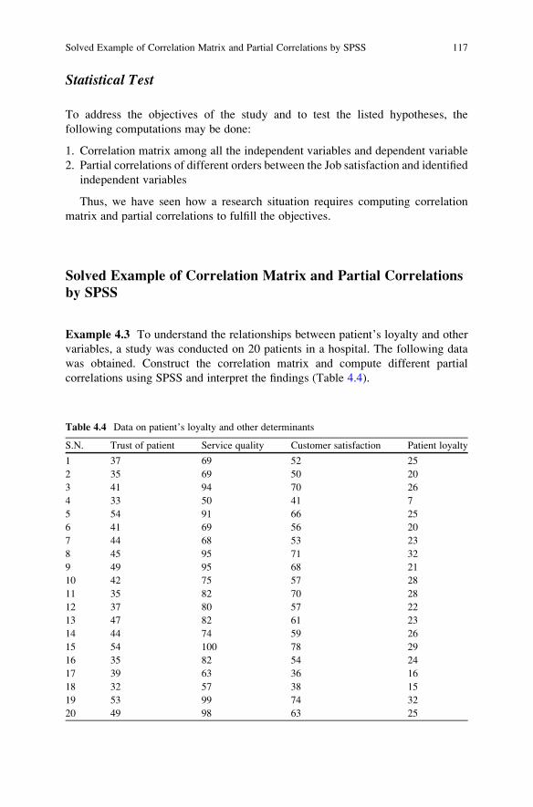
Statistical Test
To address the objectives of the study and to test the listed hypotheses, the
following computations may be done:
1. Correlation matrix among all the independent variables and dependent variable
2. Partial correlations of different orders between the Job satisfaction and identified
independent variables
Thus, we have seen how a research situation requires computing correlation
matrix and partial correlations to fulfill the objectives.
Solved Example of Correlation Matrix and Partial Correlations
by SPSS
Example 4.3 To understand the relationships between patient’s loyalty and other
variables, a study was conducted on 20 patients in a hospital. The following data
was obtained. Construct the correlation matrix and compute different partial
correlations using SPSS and interpret the findings (Table 4.4).
Table 4.4 Data on patient’s loyalty and other determinants
S.N. Trust of patient Service quality Customer satisfaction Patient loyalty
1 37 69 52 25
2 35 69 50 20
3 41 94 70 26
4 33 50 41 7
5 54 91 66 25
6 41 69 56 20
7 44 68 53 23
8 45 95 71 32
9 49 95 68 21
10 42 75 57 28
11 35 82 70 28
12 37 80 57 22
13 47 82 61 23
14 44 74 59 26
15 54 100 78 29
16 35 82 54 24
17 39 63 36 16
18 32 57 38 15
19 53 99 74 32
20 49 98 63 25
Solved Example of Correlation Matrix and Partial Correlations by SPSS 117

Solution First of all, correlation matrix shall be computed using SPSS. Option
shall be selected to show the significant correlation values. After selecting the
variables that shows significant correlation with the customer loyalty, partial
correlation shall be computed between customer loyalty and any of these selected
variables after controlling the effect of the remaining variables. The correlation
coefficients and partial correlations so obtained in the output using SPSS shall be
tested for their significance by using the p value.
Computation of Correlation Matrix Using SPSS
(a) Preparing Data File
Before using the SPSS commands for computing correlation matrix, the data
file is required to be prepared. The following steps will help you prepare the
data file:
(i) Starting the SPSS: Use the following command sequence to start SPSS:
Start ⟶ All Programs ⟶ IBM SPSS Statistics ⟶ IBM SPSS
Statistics 20
After checking the option Type in Data on the screen you will be taken to
the Variable View option for defining the variables in the study.
(ii) Defining variables: There are four variables, namely, Customer trust,Service quality, Customer satisfaction, and Customer loyalty that need to
be defined. Since these variables were measured on interval scale, they will
be defined as Scale variable in SPSS. Any variable measured on interval or
ratio scale is defined as Scale variable in SPSS. The procedure of defining
the variable in SPSS is as follows:
1. Click Variable View to define variables and their properties.
2. Write short name of these variables, that is, Trust, Service, Satisfaction,and Loyalty under the column heading Name.
3. Full names of these variables may be defined as Customer trust, Servicequality, Customer satisfaction, and Customer loyalty under the column
heading Label.
4. Under the column heading Measure, select the option “Scale” for all
these variables.
5. Use default entries in rest of the columns.
After defining all the variables in Variable View, the screen shall look like
Fig. 4.2.
(iii) Entering data After defining these variables in the Variable View, click
Data View on the left bottom of the screen to open the format for entering
data. For each variable, enter the data column wise. After entering data, the
screen will look like Fig. 4.3. Save the data file in the desired location
before further processing.
118 4 Correlation Matrix and Partial Correlation: Explaining Relationships
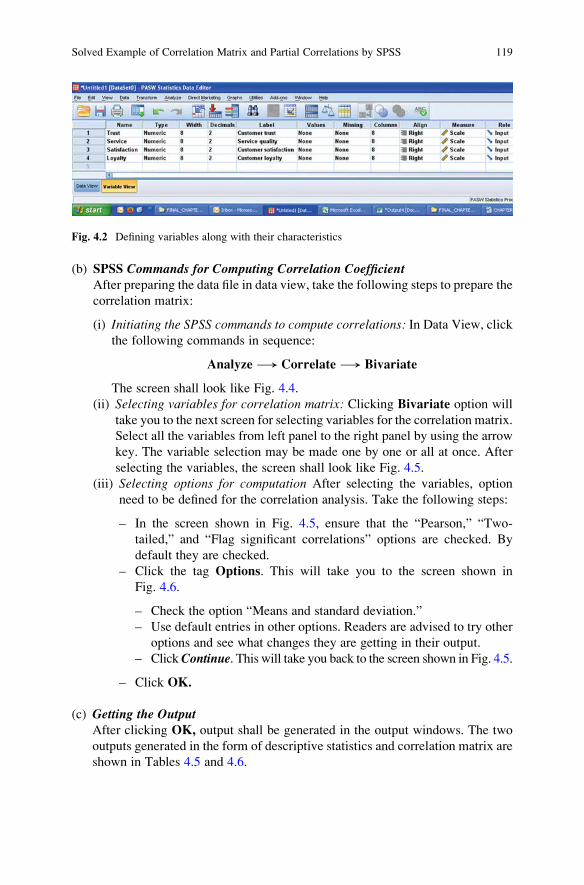
(b) SPSS Commands for Computing Correlation CoefficientAfter preparing the data file in data view, take the following steps to prepare the
correlation matrix:
(i) Initiating the SPSS commands to compute correlations: In Data View, clickthe following commands in sequence:
Analyze ⟶ Correlate ⟶ Bivariate
The screen shall look like Fig. 4.4.
(ii) Selecting variables for correlation matrix: Clicking Bivariate option will
take you to the next screen for selecting variables for the correlation matrix.
Select all the variables from left panel to the right panel by using the arrow
key. The variable selection may be made one by one or all at once. After
selecting the variables, the screen shall look like Fig. 4.5.
(iii) Selecting options for computation After selecting the variables, option
need to be defined for the correlation analysis. Take the following steps:
– In the screen shown in Fig. 4.5, ensure that the “Pearson,” “Two-
tailed,” and “Flag significant correlations” options are checked. By
default they are checked.
– Click the tag Options. This will take you to the screen shown in
Fig. 4.6.
– Check the option “Means and standard deviation.”
– Use default entries in other options. Readers are advised to try other
options and see what changes they are getting in their output.
– ClickContinue. This will take you back to the screen shown in Fig. 4.5.
– Click OK.
(c) Getting the OutputAfter clicking OK, output shall be generated in the output windows. The two
outputs generated in the form of descriptive statistics and correlation matrix are
shown in Tables 4.5 and 4.6.
Fig. 4.2 Defining variables along with their characteristics
Solved Example of Correlation Matrix and Partial Correlations by SPSS 119

Interpretation of the Outputs
The values of mean and standard deviation for all the variables are shown in
Table 4.5. The user may draw the conclusions accordingly, and the findings may
be used for further analysis in the study.
The actual output shows the full correlation matrix, but only upper diagonal
values of the correlation matrix are shown in Table 4.6. This table shows the
magnitude of correlation coefficients along with their p values and sample size.
The product moment correlation coefficient is also known as Pearson correlation as
Fig. 4.3 Scheme of data feeding for all the variables
120 4 Correlation Matrix and Partial Correlation: Explaining Relationships

Fig. 4.4 Screen showing SPSS commands for computing correlation matrix
Fig. 4.5 Screen showing selection of variables for computing correlation matrix
Solved Example of Correlation Matrix and Partial Correlations by SPSS 121

it was developed by the British mathematician Karl Pearson. The value of correla-
tion coefficient required for significance (known as critical value) at 5% as well as
at 1% level can be seen from Table A.3 in the Appendix. Thus, at 18 degrees of
freedom, the critical values of r at 5 and 1% are 0.444 and 0.561, respectively. The
correlation coefficient with one asterisk (*) mark is significant at 5% level, whereas
the one with two asterisk (**) marks shows the significance at 1% level. In this
example, the research hypothesis is two-tailed which states that “There is a signifi-
cant correlation between the two variables.” The following conclusions may be
drawn from the results in Table 4.6:
(a) The Customer loyalty is significantly correlated with customer trust at 5% level,
whereas it is significantly correlated with Service quality and Customer satis-
faction at 1% level.
(b) Customer satisfaction is highly correlated with service quality. This is rightly so
as only satisfied customers would be loyal to any hospital.
(c) All those correlation coefficients having p value less than .05 are significant at
5% level. This is shown by asterisk (*) mark by the side of the correlation
coefficient. Similarly correlations having p value less than .01 are significant at1% level, and this is indicated by two asterisk (**) marks by the side of
correlation coefficient.
Fig. 4.6 Screen showing option for computing correlation matrix and other statistics
122 4 Correlation Matrix and Partial Correlation: Explaining Relationships
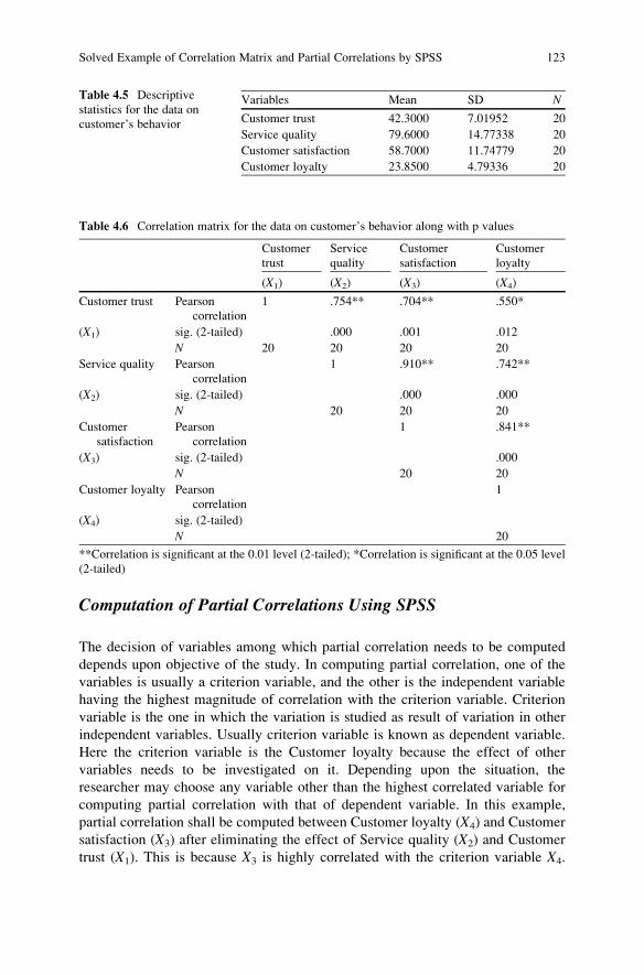
Computation of Partial Correlations Using SPSS
The decision of variables among which partial correlation needs to be computed
depends upon objective of the study. In computing partial correlation, one of the
variables is usually a criterion variable, and the other is the independent variable
having the highest magnitude of correlation with the criterion variable. Criterion
variable is the one in which the variation is studied as result of variation in other
independent variables. Usually criterion variable is known as dependent variable.
Here the criterion variable is the Customer loyalty because the effect of other
variables needs to be investigated on it. Depending upon the situation, the
researcher may choose any variable other than the highest correlated variable for
computing partial correlation with that of dependent variable. In this example,
partial correlation shall be computed between Customer loyalty (X4) and Customer
satisfaction (X3) after eliminating the effect of Service quality (X2) and Customer
trust (X1). This is because X3 is highly correlated with the criterion variable X4.
Table 4.5 Descriptive
statistics for the data on
customer’s behavior
Variables Mean SD N
Customer trust 42.3000 7.01952 20
Service quality 79.6000 14.77338 20
Customer satisfaction 58.7000 11.74779 20
Customer loyalty 23.8500 4.79336 20
Table 4.6 Correlation matrix for the data on customer’s behavior along with p values
Customer
trust
Service
quality
Customer
satisfaction
Customer
loyalty
(X1) (X2) (X3) (X4)
Customer trust Pearson
correlation
1 .754** .704** .550*
(X1) sig. (2-tailed) .000 .001 .012
N 20 20 20 20
Service quality Pearson
correlation
1 .910** .742**
(X2) sig. (2-tailed) .000 .000
N 20 20 20
Customer
satisfaction
Pearson
correlation
1 .841**
(X3) sig. (2-tailed) .000
N 20 20
Customer loyalty Pearson
correlation
1
(X4) sig. (2-tailed)
N 20
**Correlation is significant at the 0.01 level (2-tailed); *Correlation is significant at the 0.05 level
(2-tailed)
Solved Example of Correlation Matrix and Partial Correlations by SPSS 123

The decision of eliminating the effect of variables X2 and X1 has been taken because
both these variables are significantly correlated with the criterion variable. How-
ever, one can investigate the relationship between X4 vs. X2 after eliminating the
effect of the variables X3 and X1. Similarly partial correlation between X4 vs. X1
may also be investigated after eliminating the effect of the variables X3 and X2. The
procedure of computing these partial correlations with SPSS has been discussed in
the following sections:
(a) Data File for Computing Partial CorrelationThe data file which was prepared for computing correlation matrix shall be used
for computing the partial correlations. Thus, procedure for defining the
variables and entering the data for all the variables is exactly the same as was
done in case of computing correlation matrix.
(b) SPSS Commands for Partial CorrelationAfter entering all the data in the data view, take the following steps for
computing partial correlation:
(i) Initiating the SPSS commands for partial correlation: In Data View, go tothe following commands in sequence:
Analyze ⟶ Correlate ⟶ Partial
The screen shall look like Fig. 4.7.
(ii) Selecting variables for partial correlation:After clicking the Partial option,you will get the next screen for selecting variables for the partial correlation.
– Select the two variables Customer loyalty (X4) and Customer satisfac-tion (X3) from the left panel to the “Variables” section in the right panel.
Here, relationship between the variables X4 and X3 needs to be
computed after controlling the effects of Service quality (X2) and
Customer trust (X1).
– Select the variables Service quality (X2) and Customer trust (X1) from
the left panel to the “Controlling for” section in the right panel. X2 and
X1 are the two variables whose effects are to be eliminated.
The selection of variables is made either one by one or all at once. To do
so, the variable needs to be selected from the left panel, and by arrow
command, it may be brought to the right panel. The screen shall look like
Fig. 4.8.
(iii) Selecting options for computation: After selecting the variables for partial
correlation and identifying controlling variables, option needs to be defined
for the computation of partial correlation. Take the following steps:
– In the screen shown in Fig. 4.8, ensure that the options “Two-tailed”
and “Display actual significance level” are checked. By default they are
checked.
– Click the tag Options; you will get the screen as shown in Fig. 4.9.
Take the following steps:
– Check the box of “Means and standard deviations.”
124 4 Correlation Matrix and Partial Correlation: Explaining Relationships

– Use the default entries in other options. Readers are advised to try
other options and see what changes they are getting in their outputs.
– Click Continue.
– Click OK.
(c) Getting the OutputAfter clicking OK, outputs shall be generated in the output panel. The output
panel shall have two tables: one for descriptive statistics and the other for partial
correlation. These outputs can be selected by right click of the mouse and may
be pasted in the word file. In this example, the output so generated by the SPSS
will look like as shown in Tables 4.7 and 4.8.
Interpretation of Partial Correlation
Table 4.7 shows the descriptive statistics of all the variables selected in the study.
Values of mean and standard deviations may be utilized for further analysis.
Readers may note that similar table of descriptive statistics was also obtained
while computing correlation matrix by using SPSS.
Fig. 4.7 Screen showing SPSS commands for computing partial correlations
Solved Example of Correlation Matrix and Partial Correlations by SPSS 125
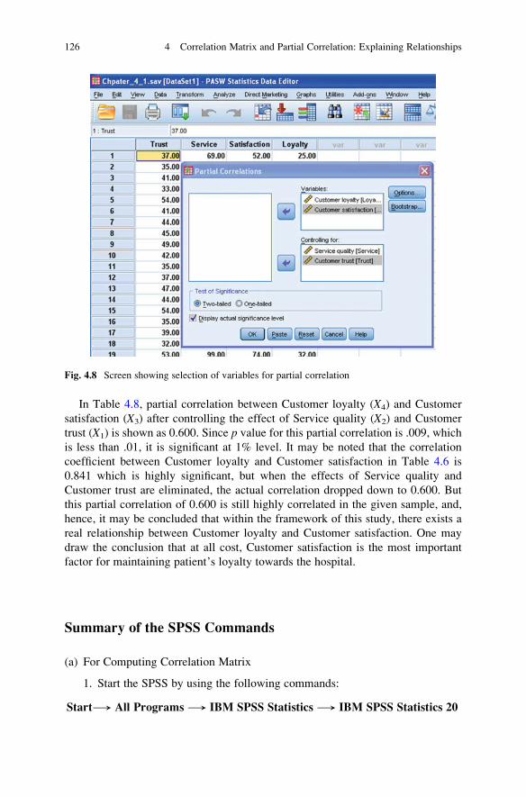
In Table 4.8, partial correlation between Customer loyalty (X4) and Customer
satisfaction (X3) after controlling the effect of Service quality (X2) and Customer
trust (X1) is shown as 0.600. Since p value for this partial correlation is .009, whichis less than .01, it is significant at 1% level. It may be noted that the correlation
coefficient between Customer loyalty and Customer satisfaction in Table 4.6 is
0.841 which is highly significant, but when the effects of Service quality and
Customer trust are eliminated, the actual correlation dropped down to 0.600. But
this partial correlation of 0.600 is still highly correlated in the given sample, and,
hence, it may be concluded that within the framework of this study, there exists a
real relationship between Customer loyalty and Customer satisfaction. One may
draw the conclusion that at all cost, Customer satisfaction is the most important
factor for maintaining patient’s loyalty towards the hospital.
Summary of the SPSS Commands
(a) For Computing Correlation Matrix
1. Start the SPSS by using the following commands:
Start⟶ All Programs ⟶ IBM SPSS Statistics ⟶ IBM SPSS Statistics 20
Fig. 4.8 Screen showing selection of variables for partial correlation
126 4 Correlation Matrix and Partial Correlation: Explaining Relationships
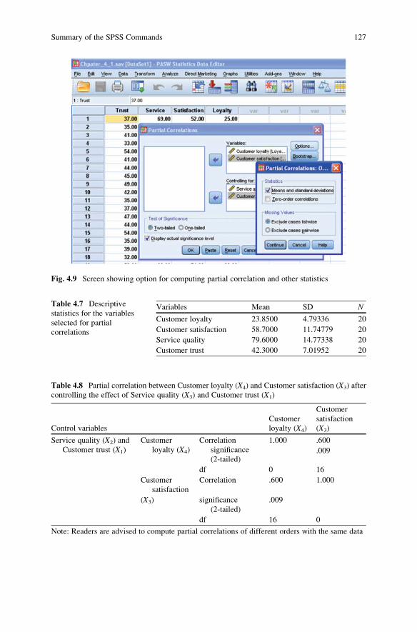
Fig. 4.9 Screen showing option for computing partial correlation and other statistics
Table 4.7 Descriptive
statistics for the variables
selected for partial
correlations
Variables Mean SD N
Customer loyalty 23.8500 4.79336 20
Customer satisfaction 58.7000 11.74779 20
Service quality 79.6000 14.77338 20
Customer trust 42.3000 7.01952 20
Table 4.8 Partial correlation between Customer loyalty (X4) and Customer satisfaction (X3) after
controlling the effect of Service quality (X3) and Customer trust (X1)
Control variables
Customer
loyalty (X4)
Customer
satisfaction
(X3)
Service quality (X2) and
Customer trust (X1)
Customer
loyalty (X4)
Correlation
significance
(2-tailed)
1.000 .600
.009
df 0 16
Customer
satisfaction
Correlation .600 1.000
(X3) significance
(2-tailed)
.009
df 16 0
Note: Readers are advised to compute partial correlations of different orders with the same data
Summary of the SPSS Commands 127
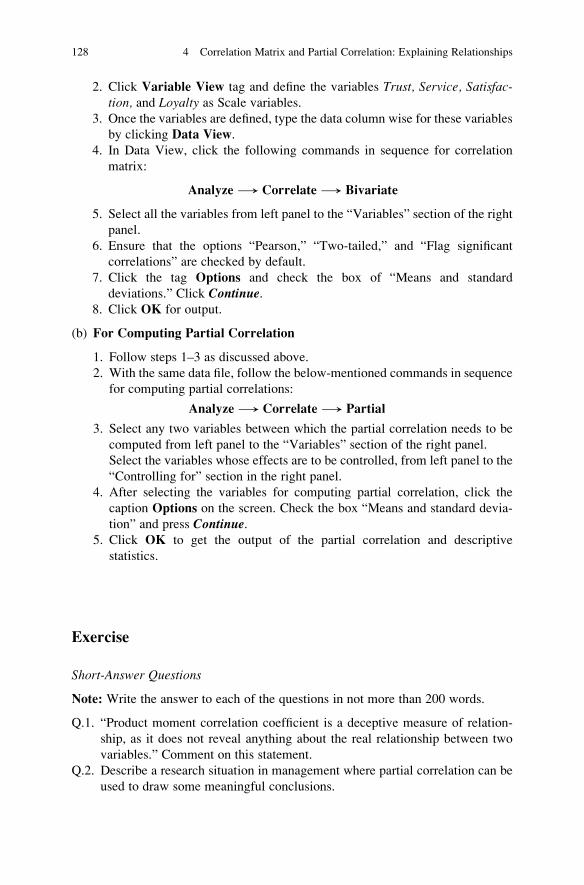
2. Click Variable View tag and define the variables Trust, Service, Satisfac-tion, and Loyalty as Scale variables.
3. Once the variables are defined, type the data column wise for these variables
by clicking Data View.
4. In Data View, click the following commands in sequence for correlation
matrix:
Analyze ⟶ Correlate ⟶ Bivariate
5. Select all the variables from left panel to the “Variables” section of the right
panel.
6. Ensure that the options “Pearson,” “Two-tailed,” and “Flag significant
correlations” are checked by default.
7. Click the tag Options and check the box of “Means and standard
deviations.” Click Continue.8. Click OK for output.
(b) For Computing Partial Correlation
1. Follow steps 1–3 as discussed above.
2. With the same data file, follow the below-mentioned commands in sequence
for computing partial correlations:
Analyze ⟶ Correlate ⟶ Partial
3. Select any two variables between which the partial correlation needs to be
computed from left panel to the “Variables” section of the right panel.
Select the variables whose effects are to be controlled, from left panel to the
“Controlling for” section in the right panel.
4. After selecting the variables for computing partial correlation, click the
caption Options on the screen. Check the box “Means and standard devia-
tion” and press Continue.5. Click OK to get the output of the partial correlation and descriptive
statistics.
Exercise
Short-Answer Questions
Note: Write the answer to each of the questions in not more than 200 words.
Q.1. “Product moment correlation coefficient is a deceptive measure of relation-
ship, as it does not reveal anything about the real relationship between two
variables.” Comment on this statement.
Q.2. Describe a research situation in management where partial correlation can be
used to draw some meaningful conclusions.
128 4 Correlation Matrix and Partial Correlation: Explaining Relationships

Q.3. Compute correlation coefficient between X and Y and interpret your findings
considering that Y and X are perfectly related by equation Y ¼ X2.
X: �3 �2 �1 0 1 2
Y: 9 4 1 0 1 4
Q.4. How will you test the significance of partial correlation using t-test?Q.5. What does the p value refer to? How is it used in testing the significance of
product moment correlation coefficient?
Multiple-Choice Questions
Note: For each of the question, there are four alternative answers. Tick mark the
one that you consider the closest to the correct answer.
1. In testing the significance of product moment correlation coefficient, degree of
freedom for t-test is
(a) N � 1
(b) N + 2
(c) N + 1
(d) N � 2
2. If the sample size increases, the value of correlation coefficient required for its
significance
(a) Increases
(b) Decreases
(c) Remains constant
(d) May increase or decrease
3. Product moment correlation coefficient measures the relationship which is
(a) Real
(b) Linear
(c) Curvilinear
(d) None of the above
4. Given that r12 ¼ 0.7 and r12.3 ¼ 0.28, where X1 is academic performance, X2 is
entrance test score, and X3 is IQ, what interpretation can be drawn?
(a) Entrance test score is an important contributory variable to the academic
performance.
(b) IQ affects the relationship between academic performance and entrance
test score in a negative fashion.
(c) IQ has got nothing to do with the academic performance.
(d) It seems there is no real relationship between academic performance and
entrance test score.
5. If p value for a partial correlation is 0.001, what conclusion can be drawn?
(a) Partial correlation is not significant at 5% level.
(b) Partial correlation is significant at 1% level.
Exercise 129

(c) Partial correlation is not significant at 1% level.
(d) Partial correlation is not significant at 10% level.
6. Partial correlation is computed with the data that are measured in
(a) Interval scale
(b) Nominal scale
(c) Ordinal scale
(d) Any scale
7. In computing correlation matrix through SPSS, all variables are defined as
(a) Nominal
(b) Ordinal
(c) Scale
(d) Any of the nominal, ordinal, or scale option depending upon the nature of
variable
8. In computing correlation matrix through SPSS, the following command
sequence is used:
(a) Analyze -> Bivariate -> Correlate
(b) Analyze -> Correlate -> Bivariate
(c) Analyze -> Correlate -> Partial
(d) Analyze -> Partial -> Bivariate
9. While selecting variables for computing partial correlation in SPSS, in
“Controlling for” section, the variables selected are
(a) All independent variables except the two between which partial correlation
is computed.
(b) Any of the independent variables as it does not affect partial correlation.
(c) Only those variables whose effects need to be eliminated.
(d) None of the above is correct.
10. The limits of partial correlation are
(a) �1 to 0
(b) 0�1
(c) Sometimes more than 1
(d) �1 to +1
Assignments
1. In a study, Job satisfaction and other organizational variables as perceived by the
employees were assessed. The data were obtained on interval scale and are
shown in the below mentioned table. Compute the following:
(a) Correlation matrix with all the seven variables
(b) Partial correlations : r12.3, r12.35, and r12.356(c) Partial correlations : r13.2, r13.25, and r13.256(d) Partial correlations : r16.2, r16.23, and r16.235
130 4 Correlation Matrix and Partial Correlation: Explaining Relationships
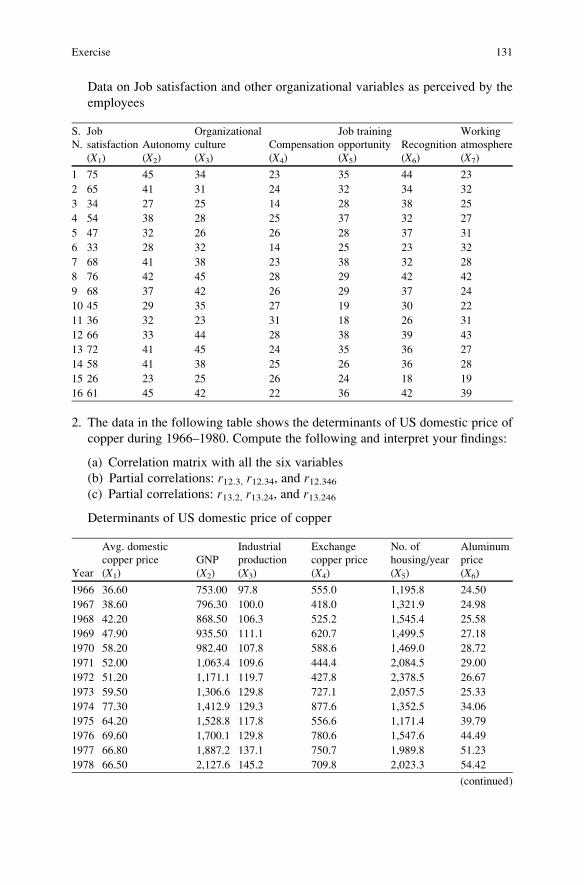
Data on Job satisfaction and other organizational variables as perceived by the
employees
S.
N.
Job
satisfaction Autonomy
Organizational
culture Compensation
Job training
opportunity Recognition
Working
atmosphere
(X1) (X2) (X3) (X4) (X5) (X6) (X7)
1 75 45 34 23 35 44 23
2 65 41 31 24 32 34 32
3 34 27 25 14 28 38 25
4 54 38 28 25 37 32 27
5 47 32 26 26 28 37 31
6 33 28 32 14 25 23 32
7 68 41 38 23 38 32 28
8 76 42 45 28 29 42 42
9 68 37 42 26 29 37 24
10 45 29 35 27 19 30 22
11 36 32 23 31 18 26 31
12 66 33 44 28 38 39 43
13 72 41 45 24 35 36 27
14 58 41 38 25 26 36 28
15 26 23 25 26 24 18 19
16 61 45 42 22 36 42 39
2. The data in the following table shows the determinants of US domestic price of
copper during 1966–1980. Compute the following and interpret your findings:
(a) Correlation matrix with all the six variables
(b) Partial correlations: r12.3, r12.34, and r12.346(c) Partial correlations: r13.2, r13.24, and r13.246
Determinants of US domestic price of copper
Year
Avg. domestic
copper price GNP
Industrial
production
Exchange
copper price
No. of
housing/year
Aluminum
price
(X1) (X2) (X3) (X4) (X5) (X6)
1966 36.60 753.00 97.8 555.0 1,195.8 24.50
1967 38.60 796.30 100.0 418.0 1,321.9 24.98
1968 42.20 868.50 106.3 525.2 1,545.4 25.58
1969 47.90 935.50 111.1 620.7 1,499.5 27.18
1970 58.20 982.40 107.8 588.6 1,469.0 28.72
1971 52.00 1,063.4 109.6 444.4 2,084.5 29.00
1972 51.20 1,171.1 119.7 427.8 2,378.5 26.67
1973 59.50 1,306.6 129.8 727.1 2,057.5 25.33
1974 77.30 1,412.9 129.3 877.6 1,352.5 34.06
1975 64.20 1,528.8 117.8 556.6 1,171.4 39.79
1976 69.60 1,700.1 129.8 780.6 1,547.6 44.49
1977 66.80 1,887.2 137.1 750.7 1,989.8 51.23
1978 66.50 2,127.6 145.2 709.8 2,023.3 54.42
(continued)
Exercise 131

(continued)
Year
Avg. domestic
copper price GNP
Industrial
production
Exchange
copper price
No. of
housing/year
Aluminum
price
(X1) (X2) (X3) (X4) (X5) (X6)
1979 98.30 2,628.8 152.5 935.7 1,749.2 61.01
1980 101.40 2,633.1 147.1 940.9 1,298.5 70.87
Note: The data were collected by Gary R. Smith from sources such as American Metal Market,
Metals Week, and US Department of Commerce publications
Answers to Multiple-Choice Questions
Q.1 d Q.2 b
Q.3 b Q.4 d
Q.5 b Q.6 a
Q.7 c Q.8 b
Q.9 c Q.10 d
132 4 Correlation Matrix and Partial Correlation: Explaining Relationships

Chapter 5
Regression Analysis and Multiple Correlations:
For Estimating a Measurable Phenomenon
Learning Objectives
After completing this chapter, you should be able to do the following:
• Explain the use of regression analysis and multiple correlation in research.
• Interpret various terms involved in regression analysis.
• Learn to use SPSS for doing regression analysis.
• Understand the procedure of identifying the most efficient regression model.
• Know the method of constructing the regression equation based on the SPSS
output.
Introduction
Regression analysis deals with estimating the value of dependent variable on the
basis of one or more independent variables. To do so, an equation is developed
between dependent and independent variables by means of least square method.
When the estimation is done on the basis of one independent variable, the procedure
is known as simple regression, and if the estimation involves more than one
independent variable, it is referred to as multiple regression analysis.
In multiple regression analysis, the dependent variable is referred to as Y,whereas independent variables are denoted as X. The dependent variable is also
known as criterion variable. The goal is to develop an equation that will determine
the Y variable in a linear function of corresponding X variables. The regression
equation can be either linear or curvilinear, but our discussion shall be limited to
linear regression only.
In regression analysis, a regression model is developed by using the observed
data obtained on dependent variable and several independent variables. During the
process, only those independent variables are picked up for developing the model
which shows significant relationship with dependent variable. Therefore, the
researcher must be careful in identifying the independent variables in regression
J.P. Verma, Data Analysis in Management with SPSS Software,DOI 10.1007/978-81-322-0786-3_5, # Springer India 2013
133

analysis study. It may be quite possible that some of the important independent
variables might have been left in the study, and, therefore, in spite of the best
possible effort, the regression model so developed may not be reliable.
Multiple regression analysis can be used in many applications of management
and behavioral researches. Numerous situations can be listed where the use of this
technique can provide an edge to the decision makers for optimum solutions.
For example, in order to evaluate and reform the existing organization and make
them more responsive to the new challenges, the management may be interested to
know; the factors responsible for sale to plan the business strategy, the estimated
number of inventory required in a given month, and the factors affecting the job
satisfaction of the employees. They may also be concerned in developing the model
for deciding the pay packets of an employee, factors that motivate people to work,
or parameters that affect the productivity of work. In all these situations, regression
model may provide the input to the management for strategic decision-making. The
success of the model depends upon the inclusion of relevant independent variables
in the study. For instance, a psychologist may like to draw up variables that directly
affect one’s mental health causing abnormal behavior. Therefore, it is important for
the researchers to review the literature thoroughly for identifying the relevant
independent variables for estimating the criterion variable.
Besides regression analysis, there are other quantitative and qualitative methods
used in performance forecasting. But the regression analysis is one of the most
popularly used quantitative techniques.
In developing a multiple regression equation, one needs to know the efficiency
in estimating the dependent variable on the basis of the identified independent
variables in the model. The efficiency of estimation is measured by the coefficient
of determination (R2) which is the square of multiple correlation. The coefficient of
determination explains the percentage of variance in the dependent variable by the
identified independent variables in the model. The multiple correlation explains the
relationship between the group of independent variables and dependent variable.
Thus, high multiple correlation ensures greater accuracy in estimating the value of
dependent variable on the basis of independent variables. Usually multiple correla-
tion, R is computed during regression analysis to indicate the validity of regression
model. It is necessary to show the value of R2 along with regression equation for
having an idea about the efficiency in prediction.
Any regression model having larger multiple correlation gives better estimates
in comparison to that of other models. We will see an explanation of the multiple
correlation while discussing the solved example later in this chapter.
Terminologies Used in Regression Analysis
In order to use the regression analysis effectively, it is essential to know different
terminologies involved in it. These terms are discussed in the following sections.
134 5 Regression Analysis and Multiple Correlations: For Estimating a Measurable. . .

Multiple Correlation
Multiple correlation is a measure of relationship between a group of independent
variables and a dependent variable. Since multiple correlation provides the strength
of relationship between dependent variable and independent variables, it is used to
determine the power of regression models also. The multiple correlation is
represented by “R” and is computed by the following formula:
R1:23 ¼ffiffiffiffiffiffiffiffiffiffiffiffiffiffiffiffiffiffiffiffiffiffiffiffiffiffiffiffiffiffiffiffiffiffiffiffiffiffiffiffiffiffiffiffiffir212 þ r213 � 2r12 r13 r23
1� r223
s(5.1)
If the number of independent variables is more than two, then the multiple
correlation is computed from the following formula:
R1:2345::::n ¼ffiffiffiffiffiffiffiffiffiffiffiffiffiffiffiffiffiffiffiffiffiffiffiffiffiffiffiffiffiffiffiffiffiffiffiffiffiffiffiffiffiffiffiffiffiffiffiffiffiffiffiffiffiffiffiffiffiffiffiffiffiffiffiffiffiffiffiffiffiffiffiffiffiffiffiffiffiffiffiffiffiffiffiffiffiffiffiffiffiffiffiffiffiffiffiffiffiffiffiffiffiffiffiffiffiffiffiffi1� ð1� r212Þð1� r213:2Þð1� r214:23Þ::::::ð1� r2
1n:23...ðn�1ÞÞq
(5.2)
where r13.2, r14.23, and r1n.234. . .(n � 1) are partial correlations.
The multiple correlation R can have the value in between 0 and +1. Since
multiple correlation is computed with the help of product moment correlation
coefficients, therefore it also measures the linear relationship only. Further, the
order of the multiple correlation is defined by n � 2, where n is the number of
variables involved in the computation of multiple correlation. Thus, the order of the
multiple correlationR12:345:::::::n is n � 2. The value of R closer to 1 indicates that the
independent variables explain most of the variations in the dependent variable. On
the other hand, if the value of R is closer to 0, it signifies that independent variables
are not capable of explaining the variation in the dependent variable. Thus, multiple
correlation can be considered to be the yardstick of efficiency in estimating the
value of dependent variable on the basis of the values of independent variables.
Properties of Multiple Correlation
1. The multiple correlation can never be lower than the highest correlation between
dependent and any of the independent variables. For instance, the value of R1.234
can never be less than the value of any of the product moment correlations r12,r13, or r14.
2. Sometimes, an independent variable does not show any relationship with depen-
dent variable, but if it is combined with some other variable, its effect becomes
significant. Such variable is known as suppression variable. These suppression
variables should be handled carefully. Thus, if the independent variables are
identified on the basis of their magnitude of correlations with the dependent
variable for developing regression line, some of the suppression variable might
Terminologies Used in Regression Analysis 135

be ignored. To handle this problem, SPSS provides the stepwise regression
method.
3. In using the stepwise regression, the variables are picked up one by one
depending upon their relative importance. Every time one variable is included,
there is an increase in multiple correlation. But the increase in multiple correla-
tion keeps on decreasing with the inclusion of every new variable. This is known
as law of diminishing return.
Example 5.1 Following is the correlation matrix obtained on the psychological
variables. Compute R1.23 and R1.234 and interpret the findings (Table 5.1):
Solution
(i)
; R1:23 ¼ffiffiffiffiffiffiffiffiffiffiffiffiffiffiffiffiffiffiffiffiffiffiffiffiffiffiffiffiffiffiffiffiffiffiffiffiffiffiffiffiffiffir212 þ r213 � 2r12r13r23
1� r223
s
Substituting values of these correlations from the correlation matrix,
R1:23 ¼ffiffiffiffiffiffiffiffiffiffiffiffiffiffiffiffiffiffiffiffiffiffiffiffiffiffiffiffiffiffiffiffiffiffiffiffiffiffiffiffiffiffiffiffiffiffiffiffiffiffiffiffiffiffiffiffiffiffiffiffiffiffiffiffiffiffiffiffiffiffiffiffiffiffiffiffiffiffiffiffiffið�0:5Þ2 þ 0:32 � 2� ð�0:5Þ � 0:3� 0:4
1� 0:42
s
¼ffiffiffiffiffiffiffiffiffi0:46
0:84
r¼ 0:74
(ii)
; R1:234 ¼ffiffiffiffiffiffiffiffiffiffiffiffiffiffiffiffiffiffiffiffiffiffiffiffiffiffiffiffiffiffiffiffiffiffiffiffiffiffiffiffiffiffiffiffiffiffiffiffiffiffiffiffiffiffiffiffiffiffiffiffiffiffiffiffiffiffiffiffiffiffiffiffiffi1� 1� r212
� �1� r213:2� �
1� r214:23� �� �q
To compute R1.234, we need to first find the values of first-order partial
correlations: r13.2, r14.2, and r43.2.
r13:2 ¼ r13 � r12r32ffiffiffiffiffiffiffiffiffiffiffiffiffiffi1� r212
p ffiffiffiffiffiffiffiffiffiffiffiffiffiffi1� r232
p ¼ 0:3� ð�0:5Þ � 0:4ffiffiffiffiffiffiffiffiffiffiffiffiffiffiffiffiffiffiffiffiffiffiffiffi1� ð�0:5Þ2
q ffiffiffiffiffiffiffiffiffiffiffiffiffiffiffiffiffi1� 0:42
p ¼ 0:50
0:79¼ 0:63
r14:2 ¼ r14 � r12r42ffiffiffiffiffiffiffiffiffiffiffiffiffiffi1� r212
p ffiffiffiffiffiffiffiffiffiffiffiffiffiffi1� r242
p ¼ 0:6� ð�0:5Þ � 0:3ffiffiffiffiffiffiffiffiffiffiffiffiffiffiffiffiffiffiffiffiffiffiffiffi1� ð�0:5Þ2
q ffiffiffiffiffiffiffiffiffiffiffiffiffiffiffiffiffi1� 0:32
p ¼ 0:75
0:83¼ 0:90
Table 5.1 Correlation matrix
of psychological variablesX1 X2 X3 X4
X1 1 �0.5 0.3 0.6
X2 1 0.4 0.3
X3 1 0.4
X4 1
X1: Memory retention, X2: Age, X3: IQ, X4: Stress level
136 5 Regression Analysis and Multiple Correlations: For Estimating a Measurable. . .
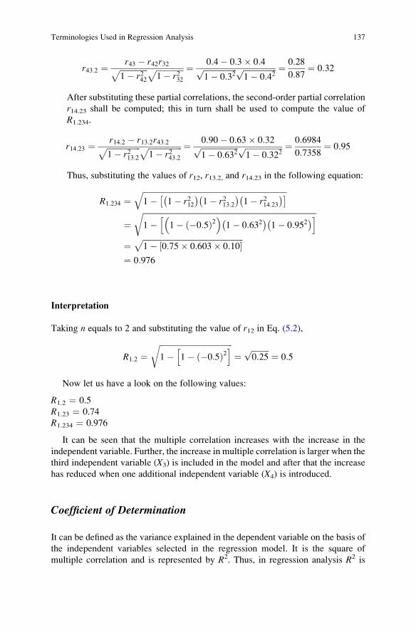
r43:2 ¼ r43 � r42r32ffiffiffiffiffiffiffiffiffiffiffiffiffiffi1� r242
p ffiffiffiffiffiffiffiffiffiffiffiffiffiffi1� r232
p ¼ 0:4� 0:3� 0:4ffiffiffiffiffiffiffiffiffiffiffiffiffiffiffiffiffi1� 0:32
p ffiffiffiffiffiffiffiffiffiffiffiffiffiffiffiffiffi1� 0:42
p ¼ 0:28
0:87¼ 0:32
After substituting these partial correlations, the second-order partial correlation
r14.23 shall be computed; this in turn shall be used to compute the value of
R1.234.
r14:23 ¼ r14:2 � r13:2r43:2ffiffiffiffiffiffiffiffiffiffiffiffiffiffiffiffiffi1� r213:2
p ffiffiffiffiffiffiffiffiffiffiffiffiffiffiffiffiffi1� r243:2
p ¼ 0:90� 0:63� 0:32ffiffiffiffiffiffiffiffiffiffiffiffiffiffiffiffiffiffiffi1� 0:632
p ffiffiffiffiffiffiffiffiffiffiffiffiffiffiffiffiffiffiffi1� 0:322
p ¼ 0:6984
0:7358¼ 0:95
Thus, substituting the values of r12, r13.2, and r14.23 in the following equation:
R1:234 ¼ffiffiffiffiffiffiffiffiffiffiffiffiffiffiffiffiffiffiffiffiffiffiffiffiffiffiffiffiffiffiffiffiffiffiffiffiffiffiffiffiffiffiffiffiffiffiffiffiffiffiffiffiffiffiffiffiffiffiffiffiffiffiffiffiffiffiffiffiffiffiffiffiffi1� 1� r212
� �1� r213:2� �
1� r214:23� �� �q
¼ffiffiffiffiffiffiffiffiffiffiffiffiffiffiffiffiffiffiffiffiffiffiffiffiffiffiffiffiffiffiffiffiffiffiffiffiffiffiffiffiffiffiffiffiffiffiffiffiffiffiffiffiffiffiffiffiffiffiffiffiffiffiffiffiffiffiffiffiffiffiffiffiffiffiffiffiffiffiffiffiffiffiffiffiffiffiffiffi1� 1� ð�0:5Þ2
� �1� 0:632� �
1� 0:952� �h ir
¼ffiffiffiffiffiffiffiffiffiffiffiffiffiffiffiffiffiffiffiffiffiffiffiffiffiffiffiffiffiffiffiffiffiffiffiffiffiffiffiffiffiffiffiffiffiffiffiffiffiffiffi1� 0:75� 0:603� 0:10½ �
p¼ 0:976
Interpretation
Taking n equals to 2 and substituting the value of r12 in Eq. (5.2),
R1:2 ¼ffiffiffiffiffiffiffiffiffiffiffiffiffiffiffiffiffiffiffiffiffiffiffiffiffiffiffiffiffiffiffiffiffiffiffiffiffi1� 1� �0:5ð Þ2
h ir¼
ffiffiffiffiffiffiffiffiffi0:25
p¼ 0:5
Now let us have a look on the following values:
R1.2 ¼ 0.5
R1.23 ¼ 0.74
R1.234 ¼ 0.976
It can be seen that the multiple correlation increases with the increase in the
independent variable. Further, the increase in multiple correlation is larger when the
third independent variable (X3) is included in the model and after that the increase
has reduced when one additional independent variable (X4) is introduced.
Coefficient of Determination
It can be defined as the variance explained in the dependent variable on the basis of
the independent variables selected in the regression model. It is the square of
multiple correlation and is represented by R2. Thus, in regression analysis R2 is
Terminologies Used in Regression Analysis 137

used for assessing the efficiency of the regression model. If for a particular
regression model R is 0.8, it means that 64% of the variability in the dependent
variable can be explained by the independent variables selected in the model.
The Regression Equation
The equation is said to be simple regression if the value of dependent variable is
estimated on the basis of one independent variable only. If Y is the dependent
variable and X is the independent variable, then the regression equation of Y on X is
written as
ðY � YÞ ¼ byxðX � XÞ (5.3)
Equation 5.3 can be used to predict the value of Y if the value of X is known.
Similarly to estimate the value of X from the value of Y, the regression equation of Xon Y shall be used which is shown in Eq. 5.4.
ðX � XÞ ¼ bxyðY � YÞ (5.4)
whereX and Y are the sample means of X and Y, respectively, and byx and bxy are theregression coefficients. These regression coefficients can be computed as
byx ¼ rsYsX
(5.5)
bxy ¼ rsXsY
(5.6)
After substituting the value of byx in Eq. (5.3) and solving, we get
Y ¼ rsYsX
X þ ðY � rsYsX
XÞ (5.7)
) Y ¼ BX þ C (5.8)
where B is equal to rsYsX
and C is (Y � rsYsX
X). The coefficients B and C are known
as unstandardized regression coefficient and regression constant respectively.
Remark Reproduce rsYsX
and (Y � rsYsX
X) in equation format. Y is the mean of Y
and X is the mean of X
After substituting the values of byx and bxy in the regression equations (5.3) and
(5.4), we get
138 5 Regression Analysis and Multiple Correlations: For Estimating a Measurable. . .

ðY � YÞ ¼ rsysx
ðX � XÞ
ðX � XÞ ¼ rsxsy
ðY � YÞ
After rearranging the above equations,
ðY � YÞsy
¼ rðX � XÞ
sx
ðX � XÞsx
¼ rðY � YÞ
sy
The above two equations can be rewritten as
Zy ¼ bxZx (5.9)
Zx ¼ byZy (5.10)
The Eqs. (5.9) and (5.10) are known as regression equations in standard score
form, and the coefficients bx and by are known as beta coefficients and are referred
to as standardized regression coefficients.
Conditions of Symmetrical Regression Equations
The two regression equations (5.3) and (5.4) are different. Equation (5.3) is known
as regression equation of Y on X and is used to estimate the value of Y on the basis of
X, whereas Eq. (5.4) is known as regression equation of X on Y and is used for
estimating the value of X if Y is known. These two equations can be rewritten as
follows:
ðY � YÞ ¼ byxðX � XÞ
ðY � YÞ ¼ 1
bxyðX � XÞ
These two regression equations can be same if the expressions in the right-hand
side of these two equations are same.
That is,
Terminologies Used in Regression Analysis 139

byxðX � XÞ ¼ 1
bxyðX � XÞ
) byx � bxy ¼ 1
) rsysx
� rsxsy
¼ 1
) r2 ¼ 1
) r ¼ �1
Hence, the two regression equations shall be similar if there is a perfect positive
or perfect negative correlation between them. In that situation, same regression
equation can be used to estimate the value of Y or value of X.
Computation of Regression Coefficient
The regression coefficient can be obtained for the given set of data by simplifying
the formula:
;B ¼ rsYsX
¼ NP
XY �PXP
YffiffiffiffiffiffiffiffiffiffiffiffiffiffiffiffiffiffiffiffiffiffiffiffiffiffiffiffiffiffiffiffiffiffiffiffiNP
X2 � ðPXÞ2q ffiffiffiffiffiffiffiffiffiffiffiffiffiffiffiffiffiffiffiffiffiffiffiffiffiffiffiffiffiffiffiffiffiffiffiffi
NP
Y2 � ðP YÞ2q �
ffiffiffiffiffiffiffiffiffiffiffiffiffiffiffiffiffiffiffiffiffiffiffiffiffiffiffiffiffiffiffiffiffiffiffiffiffi1N
PY2 �
PY
N
2sffiffiffiffiffiffiffiffiffiffiffiffiffiffiffiffiffiffiffiffiffiffiffiffiffiffiffiffiffiffiffiffiffiffiffiffiffiffi1N
PX2 �
PX
N
2s
After solving,
B ¼ NP
XY �PXP
Y
NP
X2 � PXð Þ2 (5.11)
From Eqs. (5.7) and (5.8),
C ¼ Y � rsYsX
X
After substituting the value of r sYsX
¼ B from Eq. (5.11), we get
C ¼P
Y
N� N
PXY �PX
PY
NP
X2 � ðPXÞ2 �P
X
N
After simplification,
140 5 Regression Analysis and Multiple Correlations: For Estimating a Measurable. . .
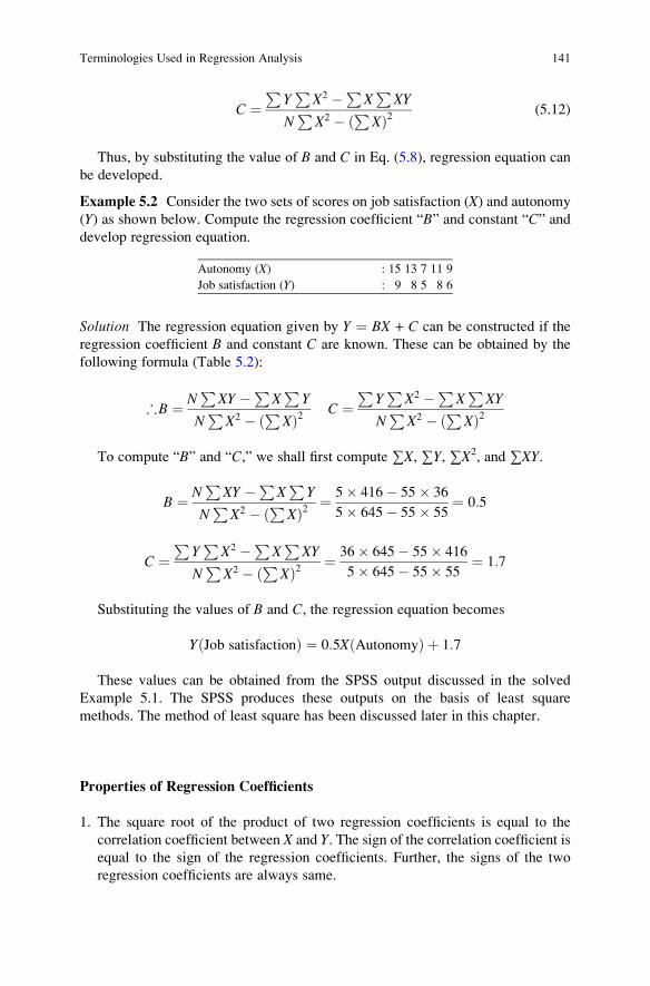
C ¼P
YP
X2 �PXP
XY
NP
X2 � ðPXÞ2 (5.12)
Thus, by substituting the value of B and C in Eq. (5.8), regression equation can
be developed.
Example 5.2 Consider the two sets of scores on job satisfaction (X) and autonomy
(Y) as shown below. Compute the regression coefficient “B” and constant “C” anddevelop regression equation.
Autonomy (X) : 15 13 7 11 9
Job satisfaction (Y) : 9 8 5 8 6
Solution The regression equation given by Y ¼ BX + C can be constructed if the
regression coefficient B and constant C are known. These can be obtained by the
following formula (Table 5.2):
;B ¼ NP
XY �PXP
Y
NP
X2 � PXð Þ2 C ¼
PYP
X2 �PXP
XY
NP
X2 � ðPXÞ2
To compute “B” and “C,” we shall first compute ∑X, ∑Y, ∑X2, and ∑XY.
B ¼ NP
XY �PXP
Y
NP
X2 � PXð Þ2 ¼ 5� 416� 55� 36
5� 645� 55� 55¼ 0:5
C ¼P
YP
X2 �PXP
XY
NP
X2 � ðPXÞ2 ¼ 36� 645� 55� 416
5� 645� 55� 55¼ 1:7
Substituting the values of B and C, the regression equation becomes
Y Job satisfactionð Þ ¼ 0:5X Autonomyð Þ þ 1:7
These values can be obtained from the SPSS output discussed in the solved
Example 5.1. The SPSS produces these outputs on the basis of least square
methods. The method of least square has been discussed later in this chapter.
Properties of Regression Coefficients
1. The square root of the product of two regression coefficients is equal to the
correlation coefficient between X and Y. The sign of the correlation coefficient isequal to the sign of the regression coefficients. Further, the signs of the two
regression coefficients are always same.
Terminologies Used in Regression Analysis 141

; byx � bxy ¼ rsysx
� rsxsy
¼ r2
) r ¼ � ffiffiffiffiffiffiffiffiffiffiffiffiffiffiffiffiffiffibyx � bxy
pTo prove that the sign of the correlation coefficient between X and Y and both
the regression coefficients are same, consider the following formula:
rxy ¼ CovðX;YÞsXsY
(5.13)
byx ¼ CovðX;YÞs2x
(5.14)
bxy ¼ CovðX;YÞs2y
(5.15)
Since sx and sy are always positive, the values of rxy, byx, and bxywill be same
and will depend upon the sign of Cov(X,Y).2. If one of the regression coefficients is greater than 1, the other will have to be
less than 1. Thus, in other words, both the regression coefficients can be less than
1 but can never be greater than 1.
We have
byx � bxy ¼ r2and� 1b r b1; byx � bxyb1) If byx>1; then bxy<1
Or if bxy>1; then byx<1
Table 5.2 Computation for
regression coefficientsScores on
Autonomy Job satisfaction
(X) (Y) X2 XY
15 9 225 135
13 8 169 104
7 5 49 35
11 8 121 88
9 6 81 54
∑X ¼ 55 ∑Y ¼ 36 ∑X2 ¼ 645 ∑XY ¼ 416
142 5 Regression Analysis and Multiple Correlations: For Estimating a Measurable. . .

Hence, the two regression coefficients cannot be simultaneously greater than
one.
3. The average of the two regression coefficients is always greater than the corre-
lation coefficient.
byx þ bxy2
>r
Least Square Method for Regression Analysis
The simple linear regression equation (5.8) is also known as least squares regression
equation. Let us plot the paired values of Xi and Yi for n sets of data; the scattergramshall look like Fig. 5.1.
The line of best fit can be represented as
Y ¼ BX þ C
where B is the slope of the line and C is the intercept on Y axis. There can be many
lines passing through these points, but the line of best fit shall be the one for which
the sum of the squares of the residuals should be least. This fact can be explained as
follows:
Each sample point has two dimensions X and Y. Thus, for ith point, Yi is the
actual value and Yi is the estimated value obtained from the line. We shall call the
line as the line of best fit if the total sum of squares is least for all these points.
XYi � Yi
� �2 ¼ Y1 � Y1
� �2 þ Y2 � Y2
� �2 þ Y3 � Y3
� �2 þ . . .þ Yn � Yn
� �2Since the criterion used for selecting the best fit line is based upon the fact that
the squares of the residuals should be least, the regression equation is known as least
square regression equation. This method of developing regression equation is
known as ordinary least square method (OLS) or simply least square method.
Fig. 5.1 Plotting of data and
the line of best fit
Terminologies Used in Regression Analysis 143
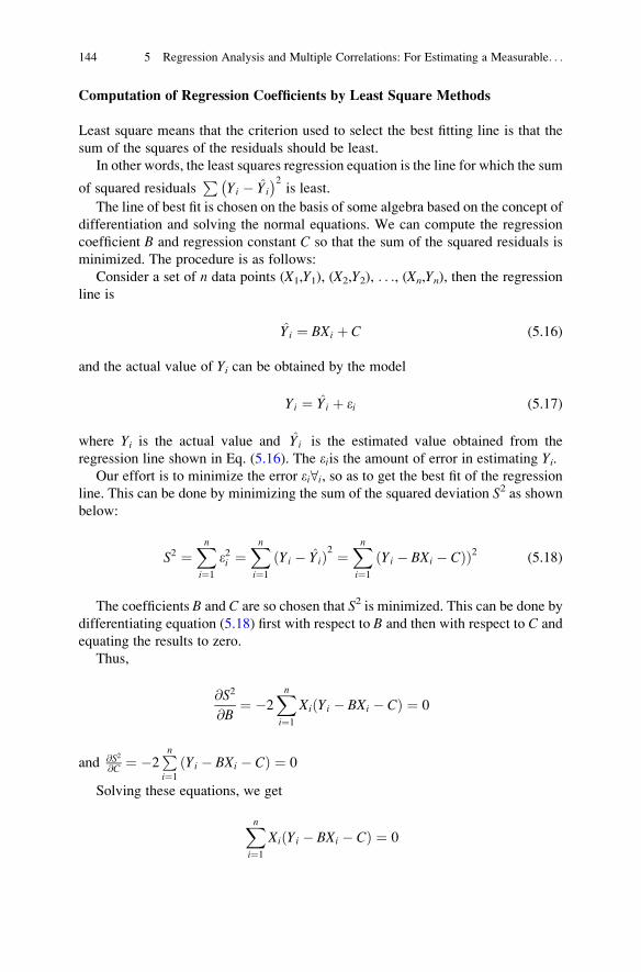
Computation of Regression Coefficients by Least Square Methods
Least square means that the criterion used to select the best fitting line is that the
sum of the squares of the residuals should be least.
In other words, the least squares regression equation is the line for which the sum
of squared residualsP
Yi � Yi
� �2is least.
The line of best fit is chosen on the basis of some algebra based on the concept of
differentiation and solving the normal equations. We can compute the regression
coefficient B and regression constant C so that the sum of the squared residuals is
minimized. The procedure is as follows:
Consider a set of n data points (X1,Y1), (X2,Y2), . . ., (Xn,Yn), then the regression
line is
Yi ¼ BXi þ C (5.16)
and the actual value of Yi can be obtained by the model
Yi ¼ Yi þ ei (5.17)
where Yi is the actual value and Yi is the estimated value obtained from the
regression line shown in Eq. (5.16). The eiis the amount of error in estimating Yi.Our effort is to minimize the error ei8i, so as to get the best fit of the regression
line. This can be done by minimizing the sum of the squared deviation S2 as shownbelow:
S2 ¼Xni¼1
e2i ¼Xni¼1
ðYi � YiÞ2 ¼Xni¼1
ðYi � BXi � CÞÞ2 (5.18)
The coefficients B and C are so chosen that S2 is minimized. This can be done by
differentiating equation (5.18) first with respect to B and then with respect to C and
equating the results to zero.
Thus,
@S2
@B¼ �2
Xni¼1
XiðYi � BXi � CÞ ¼ 0
and @S2
@C ¼ �2Pni¼1
ðYi � BXi � CÞ ¼ 0
Solving these equations, we get
Xni¼1
XiðYi � BXi � CÞ ¼ 0
144 5 Regression Analysis and Multiple Correlations: For Estimating a Measurable. . .
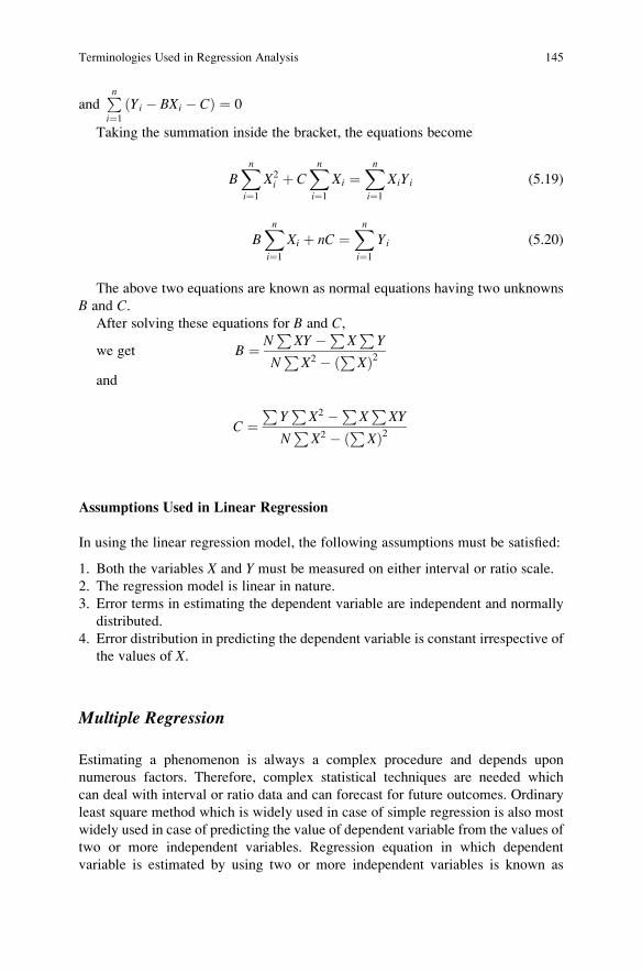
andPni¼1
ðYi � BXi � CÞ ¼ 0
Taking the summation inside the bracket, the equations become
BXni¼1
X2i þ C
Xni¼1
Xi ¼Xni¼1
XiYi (5.19)
BXni¼1
Xi þ nC ¼Xni¼1
Yi (5.20)
The above two equations are known as normal equations having two unknowns
B and C.After solving these equations for B and C,
we get B ¼ NP
XY �PXP
Y
NP
X2 � PXð Þ2
and
C ¼P
YP
X2 �PXP
XY
NP
X2 � ðPXÞ2
Assumptions Used in Linear Regression
In using the linear regression model, the following assumptions must be satisfied:
1. Both the variables X and Y must be measured on either interval or ratio scale.
2. The regression model is linear in nature.
3. Error terms in estimating the dependent variable are independent and normally
distributed.
4. Error distribution in predicting the dependent variable is constant irrespective of
the values of X.
Multiple Regression
Estimating a phenomenon is always a complex procedure and depends upon
numerous factors. Therefore, complex statistical techniques are needed which
can deal with interval or ratio data and can forecast for future outcomes. Ordinary
least square method which is widely used in case of simple regression is also most
widely used in case of predicting the value of dependent variable from the values of
two or more independent variables. Regression equation in which dependent
variable is estimated by using two or more independent variables is known as
Terminologies Used in Regression Analysis 145

multiple regression. Multiple regression equation having four independent
variables looks like
Y ¼ aþ b1X1 þ b2X2 þ b3X3 þ b4X4
where
Y is a dependent variable
X1, X2, X3, and X4 are the independent variables
a represents regression constant
b1, b2, b3, and b4 are the unstandardized regression coefficients
Procedure in Multiple Regression
In developing the multiple regression equation, independent variables must be
carefully chosen. Only those variables should be included in the study which is
supposed to explain some variation in the dependent variable. Further, one must
ensure that high degree of correlations does not exist among the independent
variables so as to avoid the multicollinearity.
The following steps are used in multiple regression analysis:
1. Compute descriptive statistics like mean, standard deviation, skewness, kurtosis,
frequency distribution, etc., and check the distribution of each variable by testing
the significance of skewness and kurtosis.
2. Assess the linearity of each independent variable with the dependent variable by
plotting the scatter diagram.
3. Check for multicollinearity among the independent variables by computing the
correlation matrix among the independent variables. If multicollinearity exists
between the independent variables then one of the independent variables must be
dropped as it does not explain additional variability in the dependent variable.
4. Develop a regression equation by using the unstandardized regression
coefficients (B coefficients).
5. Test the significance of the regression coefficients by using the t-test. As a rule ofthumb, a t-value greater than 2.0 is usually statistically significant but one must
consult a t-table to be sure.
6. Test the significance of the regression model by using the F-test. The F-value iscomputed by dividing the explained variance by the unexplained variance. In
general, an F-value of greater than 4.0 is usually statistically significant, but onemust consult an F-table to be sure.
7. Compute R2 and adjusted R2 to know the percentage variance of the dependent
variable as explained by all the independent variables together in the regression
model.
146 5 Regression Analysis and Multiple Correlations: For Estimating a Measurable. . .

Limitations of Multiple Regression
There are certain limitations of multiple regression which are as follows:
1. Like simple regression, multiple regression also will not be efficient if the
independent variables are not linearly related with dependent variable.
2. Multiple regression can be used only if the variables are either measured on
interval or ratio scale. In case the data is measured on some other scale, other
methods should be used for estimation.
3. Simple regression having one dependent and one independent variable usually
requires a minimum of 30 observations. In general, add minimum of at least 10
observations for each additional independent variable added in the study.
What Happens If the Multicollinearity Exists Among the Independent
Variables?
While doing multiple regression if multicollinearity exists, the following things
may happen:
1. The F-test for the multiple regression equation shows significance, but none of
the t-ratios for the regression coefficients will be statistically significant.
2. By adding any additional variable in the equation, the size or the sign of the
regression coefficients of other independent variables may radically change.
In case the multicollinearity is noted between any two independent variables,
one may either drop one of the two independent variables or simply show in their
findings that the multicollinearity is present.
Unstandardized and Standardized Regression Coefficients
Unstandardized regression coefficients are usually known as B coefficients,
whereas standardized regression coefficients are denoted as b(beta) coefficients.B coefficient explains the slopes of the regression lines. It indicates the amount ofchange in the dependent variable (Y) that is associated with a change in one unit
of the independent variable (X). All B coefficients are known as unstandardized
coefficients because the magnitude of their values is relative to the means and
standard deviations of the independent and dependent variables in the equation.
In other words, the slopes can be interpreted directly in terms of the raw values of Xand Y. Because the value of a B coefficient depends on the scaling of the raw data,
therefore it varies if the unit of the independent variable varies. For example, the
magnitude of B coefficient keeps changing if the unit of the independent variable
time changes as days, hours, minutes, etc. Since B coefficients depend upon the
units of the independent variables, it cannot be easily compared within a regression
equation. Thus, unstandardized regression coefficients cannot be used to find the
relative importance of the independent variables in explaining the variability of the
dependent variable in the model.
Terminologies Used in Regression Analysis 147

In order to compare the relative contribution of the independent variables in the
regression model, another type of regression coefficient, beta (b), is used. These betacoefficients are standardized coefficients such that it adjusts for the different means
and variances of the independent variables in the regression model. The standardized
regression coefficients in any regression equation are measured on the same scale on
0 to 1. Thus, these standardized regression coefficients can be directly compared to
one another, with the largest coefficient indicating the corresponding independent
variable having the maximum influence on the dependent variable.
Procedure of Multiple Regression in SPSS
In using SPSS for regression analysis, the regression coefficients are computed in the
output. Significance of these regression coefficients are tested by means of t-test. Theregression coefficient becomes significant at 5% level if its significance value
(p value) provided in the output is less than .05. Significance of regression coefficientindicates that the corresponding variable significantly explains the variation in the
dependent variable and it contributes to the regression model. F-test is computed in
the output to test the significance of overall model whereas R2 and adjusted R2 show
the percentage variability in the dependent variable as explained by all the indepen-
dent variables together in the model. Further, standardized regression coefficients are
computed in the output to find the relative predictability of the independent variables
in the model.
Methods of Regression Analysis
While doing regression analysis, the independent variables are selected either on
the basis of literature or some known information. In conducting a regression study,
a large number of independent variables are selected, and, therefore, there is a need
to identify only those independent variables which explain the maximum variation
in the dependent variable. This can be done by following any of the two methods,
namely, “stepwise regression” or “Enter” method in SPSS.
Stepwise Regression Method
This method is used in exploratory regression analysis where a larger number
of independent variables are investigated and the researcher does not have much
idea about the relationship of these variables with that of the dependent variable.
In stepwise regression analysis, the independent variables are selected one by one
depending upon the relative importance in the regression model. In other words, the
first entered variable in the model has the largest contribution in explaining variability
in the dependent variable. A variable is included in the model if its regression
coefficient is significant at 5% level. Thus, if the stepwise regression method is
selected for regression analysis, the variables are selected one by one and finally
the regression coefficients of the retained variables are generated in the output. These
regression coefficients are used to develop the required regression equation.
148 5 Regression Analysis and Multiple Correlations: For Estimating a Measurable. . .

Enter Method
This method is used in confirmatory regression analysis in which an already
developed regression model is tested for its validity on the similar sample group
for which it was earlier developed. In this procedure a regression model is devel-
oped by selecting all the independent variables in the study. The computed value of
R2 is used to assess whether the developed model is valid for the population for
which it is tested.
Application of Regression Analysis
The main focus of any industry is to maximize the profits by controlling different
strategic parameters. Optimum processes are identified, employees are motivated,
incentives are provided to sales force, and human resources are strengthened to
enhance the productivity and improve profit scenario. All these situations lead to an
exploratory study where the end result is estimated on the basis of certain indepen-
dent parameters. For instance, if one decides to knowwhat all parameters are required
to boost the sales figure in an organization, then a regression study may be planned.
The parameters like employee’s incentives, retailer’s margin, user’s schemes, prod-
uct info, advertisement expenditure, and socioeconomic status may be studied to
develop the regression model. Similarly, regression analysis may be used to identify
the parameters responsible for job satisfaction in the organization. In such case,
parameters like employee’s salary, motivation, incentives, medical facility, family
welfare incentives, and training opportunity may be selected as independent variables
for developing regression model for estimating the job satisfaction of an employee.
Regression analysis may identify independent variables which may be used for
developing strategies in production process, inventory control, capacity utilization,
sales criteria, etc. Further, regression analysis may be used to estimate the value of
dependent variable at some point of time if the values of independent variables are
known. This is more relevant in a situation where the value of dependent variable is
difficult to know. For instance, in launching a new product in a particular city, one
cannot know the sales figure, and accordingly it may affect the decision of stock
inventory. By using the regression model on sales, one can estimate the sales figure in
a particular month.
Solved Example of Multiple Regression Analysis Including
Multiple Correlation
Example 5.3 In order to assess the feasibility of a guaranteed annual wage, the
Rand Corporation conducted a study to assess the response of labor supply in terms
of average hours of work(Y) based on different independent parameters. The data
were drawn from a national sample of 6,000 households with male head earnings
less than $15,000 annually. These data are given in Table 5.3. Apply regression
Solved Example of Multiple Regression Analysis Including Multiple Correlation 149
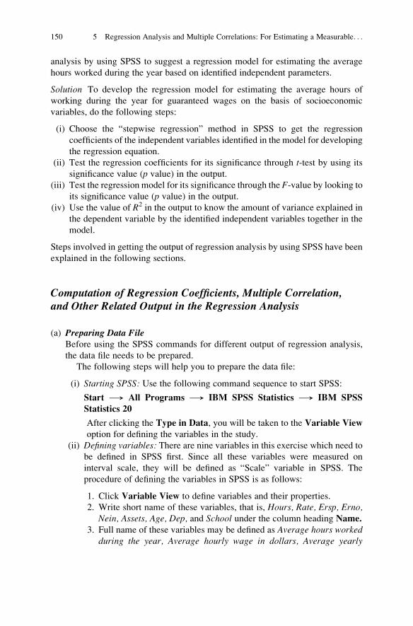
analysis by using SPSS to suggest a regression model for estimating the average
hours worked during the year based on identified independent parameters.
Solution To develop the regression model for estimating the average hours of
working during the year for guaranteed wages on the basis of socioeconomic
variables, do the following steps:
(i) Choose the “stepwise regression” method in SPSS to get the regression
coefficients of the independent variables identified in the model for developing
the regression equation.
(ii) Test the regression coefficients for its significance through t-test by using its
significance value (p value) in the output.
(iii) Test the regression model for its significance through the F-value by looking toits significance value (p value) in the output.
(iv) Use the value of R2 in the output to know the amount of variance explained in
the dependent variable by the identified independent variables together in the
model.
Steps involved in getting the output of regression analysis by using SPSS have been
explained in the following sections.
Computation of Regression Coefficients, Multiple Correlation,and Other Related Output in the Regression Analysis
(a) Preparing Data FileBefore using the SPSS commands for different output of regression analysis,
the data file needs to be prepared.
The following steps will help you to prepare the data file:
(i) Starting SPSS: Use the following command sequence to start SPSS:
Start ⟶ All Programs ⟶ IBM SPSS Statistics ⟶ IBM SPSS
Statistics 20
After clicking the Type in Data, you will be taken to the Variable View
option for defining the variables in the study.
(ii) Defining variables: There are nine variables in this exercise which need tobe defined in SPSS first. Since all these variables were measured on
interval scale, they will be defined as “Scale” variable in SPSS. The
procedure of defining the variables in SPSS is as follows:
1. Click Variable View to define variables and their properties.
2. Write short name of these variables, that is, Hours, Rate, Ersp, Erno,Nein, Assets, Age, Dep, and School under the column heading Name.
3. Full name of these variables may be defined as Average hours workedduring the year, Average hourly wage in dollars, Average yearly
150 5 Regression Analysis and Multiple Correlations: For Estimating a Measurable. . .

Table 5.3 Data on average yearly hour and other socioeconomic variables
S.N.
Hours Rate ERSP ERNO NEIN Assets Age DEP School
(X1) (X2) (X3) (X4) (X5) (X6) (X7) (X8) (X9)
1 2,157 2.905 1,121 291 380 7,250 38.5 2.340 10.5
2 2,174 2.970 1,128 301 398 7,744 39.3 2.335 10.5
3 2,062 2.350 1,214 326 185 3,068 40.1 2.851 8.9
4 2,111 2.511 1,203 49 117 1,632 22.4 1.159 11.5
5 2,134 2.791 1,013 594 730 12,710 57.7 1.229 8.8
6 2,185 3.040 1,135 287 382 7,706 38.6 2.602 10.7
7 2,210 3.222 1,100 295 474 9,338 39.0 2.187 11.2
8 2,105 2.493 1,180 310 255 4,730 39.9 2.616 9.3
9 2,267 2.838 1,298 252 431 8,317 38.9 2.024 11.1
10 2,205 2.356 885 264 373 6,789 38.8 2.662 9.5
11 2,121 2.922 1,251 328 312 5,907 39.8 2.287 10.3
12 2,109 2.499 1,207 347 271 5,069 39.7 3.193 8.9
13 2,108 2.796 1,036 300 259 4,614 38.2 2.040 9.2
14 2,047 2.453 1,213 297 139 1,987 40.3 2.545 9.1
15 2,174 3.582 1,141 414 498 10,239 40.0 2.064 11.7
16 2,067 2.909 1,805 290 239 4,439 39.1 2.301 10.5
17 2,159 2.511 1,075 289 308 5,621 39.3 2.486 9.5
18 2,257 2.516 1,093 176 392 7,293 37.9 2.042 10.1
19 1,985 1.423 553 381 146 1,866 40.6 3.833 6.6
20 2,184 3.636 1,091 291 560 11,240 39.1 2.328 11.6
21 2,084 2.983 1,327 331 296 5,653 39.8 2.208 10.2
22 2,051 2.573 1,194 279 172 2,806 40.0 2.362 9.1
23 2,127 3.262 1,226 314 408 8,042 39.5 2.259 10.8
24 2,102 3.234 1,188 414 352 7,557 39.8 2.019 10.7
25 2,098 2.280 973 364 272 4,400 40.6 2.661 8.4
26 2,042 2.304 1,085 328 140 1,739 41.8 2.444 8.2
27 2,181 2.912 1,072 304 383 7,340 39.0 2.337 10.2
28 2,186 3.015 1,122 30 352 7,292 37.2 2.046 10.9
29 2,188 3.010 990 366 374 7,325 38.4 2.847 10.6
30 2,077 1.901 350 209 951 370 37.4 4.158 8.2
31 2,196 3.009 947 294 342 6,888 37.5 3.047 10.6
32 2,093 1.899 342 311 120 1,425 37.5 4.512 8.1
33 2,173 2.959 1,116 296 387 7,625 39.2 2.342 10.5
34 2,179 2.971 1,128 312 397 7,779 39.4 2.341 10.5
35 2,200 2.980 1,126 204 393 7,885 39.2 2.341 10.6
Source: D. H. Greenberg and M. Kosters, Income Guarantees and the Working Poor, The Rand
Corporation, R-579-OEO, December 1970.
Hours(X1): average hours worked during the year
Rate(X2): average hourly wage (dollars)
ERSP(X3): average yearly earnings of spouse (dollars)
ERNO(X4): average yearly earnings of other family members (dollars)
NEIN(X5): average yearly non-earned income
Assets(X6): average family asset holdings (bank account) (dollars)
Age(X7): average age of respondent
Dep(X8): average number of dependents
School(X9): average highest grade of school completed
Solved Example of Multiple Regression Analysis Including Multiple Correlation 151

earnings of spouse in dollars, Average yearly earnings of other familymembers in dollars, Average yearly non-earned income, Averagefamily asset holdings (bank account, etc.) in dollars, Average age ofrespondent, Average number of dependents, and Average highestgrade of school completed under the column heading Label.
4. Under the column heading Measure, select the option “Scale” for all
these variables.
5. Use default entries in all other columns.
After defining these variables in variable view, the screen shall look like
Fig. 5.2.
(iii) Entering data: After defining these variables in the Variable View, click
Data View on the left bottom of the screen to enter data. For each variable,
enter the data column wise. After entering data, the screen will look like
Fig. 5.3. Save the data file in the desired location before further processing.
(b) SPSS Commands for Computing Correlation CoefficientAfter preparing the data file in data view, take the following steps for regression
analysis. Data file in SPSS can also be prepared by transporting the data from
the other format like EXCEL or ASCII. The procedure of transporting data
from other formats has been explained in Chap. 1.
(i) Initiating the SPSS commands for regression analysis: In data view, choosethe following commands in sequence:
Analyze⟶ Regression⟶Linear
The screen shall look like Fig. 5.4.
(ii) Selecting variables for regression analysis: After clicking the Linear
option, you will be taken to the next screen as shown in Fig. 5.5 for
selecting the variables for regression analysis. Select the variable Averagehours worked during the year (dependent variable) from left panel to the
“Dependent” section of the right panel. Select all independent variables
from left panel to the “Independent(s)” section of the right panel.
Fig. 5.2 Defining variables along with their characteristics
152 5 Regression Analysis and Multiple Correlations: For Estimating a Measurable. . .
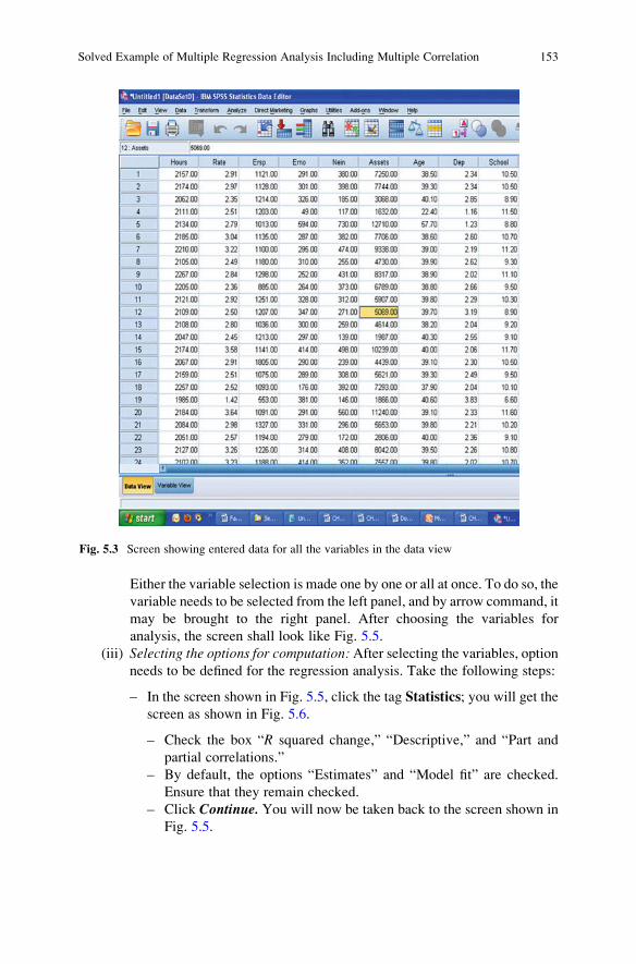
Either the variable selection is made one by one or all at once. To do so, the
variable needs to be selected from the left panel, and by arrow command, it
may be brought to the right panel. After choosing the variables for
analysis, the screen shall look like Fig. 5.5.
(iii) Selecting the options for computation: After selecting the variables, optionneeds to be defined for the regression analysis. Take the following steps:
– In the screen shown in Fig. 5.5, click the tag Statistics; you will get the
screen as shown in Fig. 5.6.
– Check the box “R squared change,” “Descriptive,” and “Part and
partial correlations.”
– By default, the options “Estimates” and “Model fit” are checked.
Ensure that they remain checked.
– Click Continue. You will now be taken back to the screen shown in
Fig. 5.5.
Fig. 5.3 Screen showing entered data for all the variables in the data view
Solved Example of Multiple Regression Analysis Including Multiple Correlation 153
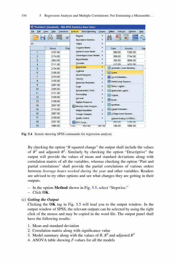
By checking the option “R squared change” the output shall include the values
of R2 and adjusted R2. Similarly by checking the option “Descriptive” the
output will provide the values of mean and standard deviations along with
correlation matrix of all the variables, whereas checking the option “Part and
partial correlations” shall provide the partial correlations of various orders
between Average hours worked during the year and other variables. Readers
are advised to try other options and see what changes they are getting in their
outputs.
– In the option Method shown in Fig. 5.5, select “Stepwise.”
– Click OK.
(c) Getting the OutputClicking the OK tag in Fig. 5.5 will lead you to the output window. In the
output window of SPSS, the relevant outputs can be selected by using the right
click of the mouse and may be copied in the word file. The output panel shall
have the following results:
1. Mean and standard deviation
2. Correlation matrix along with significance value
3. Model summary along with the values of R, R2 and adjusted R2
4. ANOVA table showing F-values for all the models
Fig. 5.4 Screen showing SPSS commands for regression analysis
154 5 Regression Analysis and Multiple Correlations: For Estimating a Measurable. . .

5. Standardized and unstandardized regression coefficients of selected variables
in different models along with their t-values and partial correlations
In this example, all the outputs so generated by the SPSS have been shown in
Tables 5.4, 5.5, 5.6, 5.7, and 5.8.
Interpretation of the Outputs
Different outputs generated in the SPSS are shown below along with their
interpretations.
1. The values of mean and standard deviation for all the variables are shown in
Table 5.4. These values can be used for further analysis in the study. By using
the procedure discussed in Chap. 2, a profile chart may be prepared by comput-
ing other descriptive statistics for all the variables.
2. The correlation matrix in Table 5.5 shows the correlations among the variables
along with their significance value (p value). Significance of these correlations
has been tested for one-tailed test. The correlation coefficient with one asterisk
Fig. 5.5 Screen showing selection of variables for regression analysis
Solved Example of Multiple Regression Analysis Including Multiple Correlation 155

mark (*) indicates its significance at 5% level. The asterisk mark (*) is put on the
correlation coefficient if its value is more than the required value of correlation
coefficients for its significance at 5% level which is .284. For one-tailed test, the
required value of “r” for significance with 33 (N � 2) df can be seen from
Table A.3 in the Appendix.
Fig. 5.6 Screen showing options for computing various components of regression analysis
Table 5.4 Descriptive statistics for different variables
Variables Mean SD N
Average hours worked during the year 2,137.09 64.12 35
Average hourly wage 2.74 .46 35
Average yearly earnings of spouse 1,083.66 256.78 35
Average yearly earnings of other family members 298.23 94.99 35
Average yearly non-earned income 348.23 167.59 35
Average family asset holdings 6,048.14 2,921.40 35
Average age of respondent 39.24 4.40 35
Average number of dependents 2.49 .66 35
Average highest grade of school completed 9.92 1.17 35
156 5 Regression Analysis and Multiple Correlations: For Estimating a Measurable. . .

Similarly for one-tailed test, the significance value for the correlation coefficient
at .01 level with 33 (¼N � 2) df can be seen as 0.392. Thus, all those correlation
coefficients having valuesmore than 0.392 are significant at 1% level. Such correla-
tion coefficients have been shown with two asterisk marks (**).
Readers may also show the correlation matrix by writing the upper diagonal
values as has been done in Chap. 4.
3. From Table 5.5, it can be seen that Hours (Average hours worked during the
year) is significantly correlated with Rate (Average hourly wage), Nein (Averageyearly non-earned income), Assets (Average family asset holdings), and School(Average highest grade of school completed) at 1% level, whereas with Dep(Average number of dependents) at 5% level.
Table 5.5 Correlation matrix for different variables along with significance level
Hours Rate Ersp Erno Nein Assets Age Dep School
Pearson correlation
Hours 1.000 .556** .124 �.245 .413** .716** �.077 �.339* .681**
Rate .556** 1.000 .572** .059 .297* .783** .044 �.601** .881**
Ersp .124 .572** 1.000 �.041 �.238 .298* �.015 �.693** .549**
Erno �.245 .059 �.041 1.000 .152 .296* .775** .050 �.299*
Nein .413** .297* �.238 .152 1.000 .512** .347* �.045 .219
Assets .716** .783** .298* .296* .512** 1.000 .414** �.530** .634**
Age �.077 .044 �.015 .775** .347* .414** 1.000 �.048 �.331
Dep �339* �.601** �.693** .050 �.045 �.530** �.048 1.000 �.603**
School .681** .881** .549** �.299* .219 .634** �.331* �.603** 1.000
Sig. (1-tailed)
Hours .000 .239 .078 .007 .000 .330 .023 .000
Rate .000 . .000 .368 .041 .000 .401 .000 .000
Ersp .239 .000 . .408 .084 .041 .465 .000 .000
Erno .078 .368 .408 . .192 .042 .000 .387 .041
Nein .007 .041 .084 .192 . .001 .021 .398 .103
Assets .000 .000 .041 .042 .001 . .007 .001 .000
Age .330 .401 .465 .000 .021 .007 . .391 .026
Dep .023 .000 .000 .387 .398 .001 .391 . .000
School .000 .000 .000 .041 .103 .000 .026 .000 .
Hours: Average hours worked during the year
Rate: Average hourly wage
Ersp: Average yearly earnings of spouse
Erno: Average yearly earnings of other family members
Nein: Average yearly non-earned income
Assets: Average family asset holdings
Age: Average age of respondentDep: Average number of dependents
School: Average highest grade of school completed
*Significant at 0.05 level (1-tailed) Significant value of r at .05 level with 33 df (1-tailed) ¼ 0.284;
**Significant at 0.01 level (1-tailed) Significant value of r at .01 level with 33 df (1-
tailed) ¼ 0.392
Solved Example of Multiple Regression Analysis Including Multiple Correlation 157
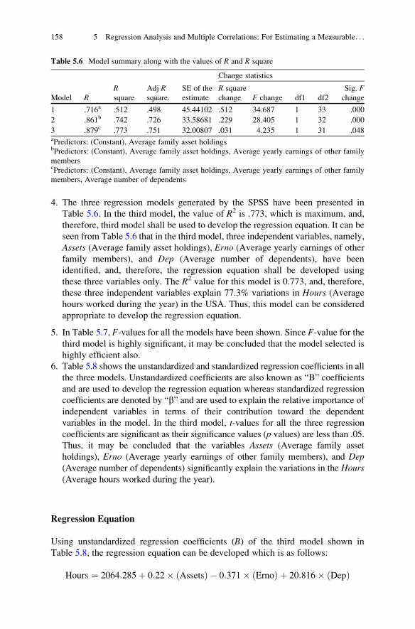
4. The three regression models generated by the SPSS have been presented in
Table 5.6. In the third model, the value of R2 is .773, which is maximum, and,
therefore, third model shall be used to develop the regression equation. It can be
seen from Table 5.6 that in the third model, three independent variables, namely,
Assets (Average family asset holdings), Erno (Average yearly earnings of other
family members), and Dep (Average number of dependents), have been
identified, and, therefore, the regression equation shall be developed using
these three variables only. The R2 value for this model is 0.773, and, therefore,
these three independent variables explain 77.3% variations in Hours (Averagehours worked during the year) in the USA. Thus, this model can be considered
appropriate to develop the regression equation.
5. In Table 5.7, F-values for all the models have been shown. Since F-value for thethird model is highly significant, it may be concluded that the model selected is
highly efficient also.
6. Table 5.8 shows the unstandardized and standardized regression coefficients in all
the three models. Unstandardized coefficients are also known as “B” coefficients
and are used to develop the regression equation whereas standardized regression
coefficients are denoted by “b” and are used to explain the relative importance of
independent variables in terms of their contribution toward the dependent
variables in the model. In the third model, t-values for all the three regression
coefficients are significant as their significance values (p values) are less than .05.Thus, it may be concluded that the variables Assets (Average family asset
holdings), Erno (Average yearly earnings of other family members), and Dep(Average number of dependents) significantly explain the variations in the Hours(Average hours worked during the year).
Regression Equation
Using unstandardized regression coefficients (B) of the third model shown in
Table 5.8, the regression equation can be developed which is as follows:
Hours ¼ 2064:285þ 0:22� Assetsð Þ � 0:371� Ernoð Þ þ 20:816� Depð Þ
Table 5.6 Model summary along with the values of R and R square
Change statistics
Model RRsquare
Adj Rsquare.
SE of the
estimate
R square
change F change df1 df2
Sig. Fchange
1 .716a .512 .498 45.44102 .512 34.687 1 33 .000
2 .861b .742 .726 33.58681 .229 28.405 1 32 .000
3 .879c .773 .751 32.00807 .031 4.235 1 31 .048aPredictors: (Constant), Average family asset holdingsbPredictors: (Constant), Average family asset holdings, Average yearly earnings of other family
memberscPredictors: (Constant), Average family asset holdings, Average yearly earnings of other family
members, Average number of dependents
158 5 Regression Analysis and Multiple Correlations: For Estimating a Measurable. . .

where
Hours: Average hours worked during the year
Assets: Average family asset holdings
Erno: Average yearly earnings of other family members
Dep: Average number of dependents
Thus, it may be concluded that the above regression equation is quite reliable as
the value of R2 is 0.773. In other words, the three variables selected in this
regression equation explain 77.3% of the total variability in the Hour (Average
hours worked during the year), which is quite good. Since the F-value for this
regression model is highly significant, the model is reliable. At the same time, all
the regression coefficients in this model are highly significant, and, therefore, it may
be interpreted that all the three variables selected in the model, namely, Assets(Average family asset holdings), Erno (Average yearly earnings of other family
members), and Dep (Average number of dependents), have significant predictabil-
ity in estimating the value of the Hour (Average hours worked during the year) in
the USA.
Summary of the SPSS Commands For Regression Analysis
1. Start SPSS by using the following commands:
Start ⟶ All Programs ⟶ IBM SPSS Statistics ⟶ IBM SPSS Statistics
2. Create data file by clicking the tag Type in Data. Define all the variables and
their characteristics by clicking the Variable View. After defining the variables,
type the data for these variables by clicking Data View.
Table 5.7 ANOVA table showing F-values for all the modelsa
Model Sum of squares df Mean square F Sig.
1 Regression 71,625.498 1 71,625.498 34.687 .000b
Residual 68,141.245 33 2,064.886
Total 139,766.743 34
2 Regression 103,668.390 2 51,834.195 45.949 .000c
Residual 36,098.353 32 1,128.074
Total 139,766.743 34
3 Regression 108,006.736 3 36,002.245 35.141 .000d
Residual 31,760.007 31 1,024.516
Total 139,766.743 34aDependent variable: Average hours worked during the yearbPredictors: (Constant), Average family asset holdingscPredictors: (Constant), Average family asset holdings, Average yearly earnings of other family
membersdPredictors: (Constant), Average family asset holdings, Average yearly earnings of other family
members, Average number of dependents
Summary of the SPSS Commands For Regression Analysis 159
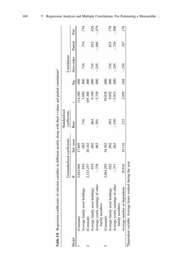
Table
5.8
Regressioncoefficientsofselected
variablesin
differentmodelsalongwiththeirt-values
andpartial
correlationsa
Model
Unstandardized
coefficients
Standardized
coefficients
Correlations
BStd.error
Beta
tSig.
Zero-order
Partial
Part
1(Constant)
2,042.064
17.869
114.280
.000
Averagefamilyassetholdings
.016
.003
.716
5.890
.000
.716
.716
.716
2(Constant)
2,123.257
20.162
105.308
.000
Averagefamilyassetholdings
.019
.002
.864
9.190
.000
.716
.852
.826
Averageyearlyearningsofother
familymem
bers
�.338
.063
�.501
�5.330
.000
�.245
�.686
�.479
3(Constant)
2,064.285
34.503
59.828
.000
Averagefamilyassetholdings
.022
.002
.993
9.092
.000
.716
.853
.778
Averageyearlyearningsofother
familymem
bers
�.371
.063
�.550
�5.933
.000
�.245
�.729
�.508
Averagenumber
ofdependents
20.816
10.116
.215
2.058
.048
�.339
.347
.176
aDependentvariable:Averagehoursworked
duringtheyear
160 5 Regression Analysis and Multiple Correlations: For Estimating a Measurable. . .

3. Once the data file is ready, use the following command sequence for selecting
the variables for analysis.
Analyze ! Regression ! Linear
4. Select the dependent variable from left panel to the “Dependent” section of the
right panel. Select all other independent variables from left panel to the “Inde-
pendent(s)” section of the right panel.
5. After selecting the variables for regression analysis, click the tag Statistics on
the screen. Check the box “R squared change,” “Descriptive,” and “Part and
partial correlations.” Press Continue.6. In the Method option, select “Stepwise,” then press OK to get the different
outputs for regression analysis.
Exercise
Short-Answer Questions
Note: Write answer to each of the questions in not more than 200 words.
Q.1. Describe regression analysis. Explain the difference between simple regres-
sion and multiple regression models.
Q.2. What is the difference between stepwise regression and backward regression?
Q.3. Discuss the role of R2 in regression analysis. Explain multiple correlation and
its order.
Q.4. Explain an experimental situation where regression analysis can be used.
Q.5. How will you know that the variables which are selected in the regression
analysis are valid?
Q.6. What is the difference between Stepwise and Enter method in developing
multiple regression equation?
Multiple-Choice Questions
Note: For each of the question, there are four alternative answers. Tick mark the
one that you consider the closest to the correct answer.
1. The range of multiple correlation R is
(a) �1 to 0
(b) 0 to 1
(c) �1 to 0
(d) None of the above
2. SPSS commands for multiple regression analysis is
(a) Analyze -> Linear -> Regression
(b) Analyze -> Regression -> Linear
(c) Analyze -> Linear Regression
(d) Analyze -> Regression Linear
Exercise 161
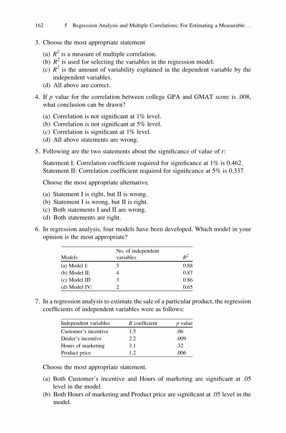
3. Choose the most appropriate statement
(a) R2 is a measure of multiple correlation.
(b) R2 is used for selecting the variables in the regression model.
(c) R2 is the amount of variability explained in the dependent variable by the
independent variables.
(d) All above are correct.
4. If p value for the correlation between college GPA and GMAT score is .008,
what conclusion can be drawn?
(a) Correlation is not significant at 1% level.
(b) Correlation is not significant at 5% level.
(c) Correlation is significant at 1% level.
(d) All above statements are wrong.
5. Following are the two statements about the significance of value of r:
Statement I: Correlation coefficient required for significance at 1% is 0.462.
Statement II: Correlation coefficient required for significance at 5% is 0.337.
Choose the most appropriate alternative.
(a) Statement I is right, but II is wrong.
(b) Statement I is wrong, but II is right.
(c) Both statements I and II are wrong.
(d) Both statements are right.
6. In regression analysis, four models have been developed. Which model in your
opinion is the most appropriate?
Models
No. of independent
variables R2
(a) Model I: 5 0.88
(b) Model II: 4 0.87
(c) Model III: 3 0.86
(d) Model IV: 2 0.65
7. In a regression analysis to estimate the sale of a particular product, the regression
coefficients of independent variables were as follows:
Independent variables B coefficient p value
Customer’s incentive 1.5 .06
Dealer’s incentive 2.2 .009
Hours of marketing 3.1 .32
Product price 1.2 .006
Choose the most appropriate statement.
(a) Both Customer’s incentive and Hours of marketing are significant at .05
level in the model.
(b) Both Hours of marketing and Product price are significant at .05 level in the
model.
162 5 Regression Analysis and Multiple Correlations: For Estimating a Measurable. . .

(c) Both Dealer’s incentive and Product price are significant at .01 level in the
model.
(d) Both Dealer’s incentive and Product price are not significant at .05 level in
the model.
8. Choose correct statement about B and b coefficients.
(a) “B” is an unstandardized coefficient and “b” is a standardized coefficient.
(b) “b” is an unstandardized coefficient and “B” is a standardized coefficient.
(c) Both “B” and “b” are standardized coefficients.
(d) Both “B” and “b” are unstandardized coefficients.
Assignments
1. The data on copper industry and its determinants in the US market during
1951–1980 are shown in the following table. Construct a regression model and
develop the regression equation by using the SPSS. Test the significance of
regression coefficients and explain the robustness of the regression model to
predict the price of the copper in the US market.
Determinants of US domestic price of copper
DPC GNP IIP MEPC NOH PA
21.89 330.2 45.1 220.4 1,491.00 19.00
22.29 347.2 50.9 259.5 1,504.00 19.41
19.63 366.1 53.3 256.3 1,438.00 20.93
22.85 366.3 53.6 249.3 1,551.00 21.78
33.77 399.3 54.6 352.3 1,646.00 23.68
39.18 420.7 61.1 329.1 1,349.00 26.01
30.58 442.0 61.9 219.6 1,224.00 27.52
26.30 447.0 57.9 234.8 1,382.00 26.89
30.70 483.0 64.8 237.4 1,553.70 26.85
32.10 506.0 66.2 245.8 1,296.10 27.23
30.00 523.3 66.7 229.2 1,365.00 25.46
30.80 563.8 72.2 233.9 1,492.50 23.88
30.80 594.7 76.5 234.2 1,634.90 22.62
32.60 635.7 81.7 347.0 1,561.00 23.72
35.40 688.1 89.8 468.1 1,509.70 24.50
36.60 753.0 97.8 555.0 1,195.80 24.50
38.60 796.3 100.0 418.0 1,321.90 24.98
42.20 868.5 106.3 525.2 1,545.40 25.58
47.90 935.5 111.1 620.7 1,499.50 27.18
58.20 982.4 107.8 588.6 1,469.00 28.72
52.00 1,063.4 109.6 444.4 2,084.50 29.00
51.20 1,171.1 119.7 427.8 2,378.50 26.67
59.50 1,306.6 129.8 727.1 2,057.50 25.33
77.30 1,412.9 129.3 877.6 1,352.50 34.06
64.20 1,528.8 117.8 556.6 1,171.40 39.79
69.60 1,700.1 129.8 780.6 1,547.60 44.49
66.80 1,887.2 137.1 750.7 1,989.80 51.23
(continued)
Exercise 163

(continued)
Determinants of US domestic price of copper
DPC GNP IIP MEPC NOH PA
66.50 2,127.6 145.2 709.8 2,023.30 54.42
98.30 2,628.80 152.5 935.7 1,749.20 61.01
101.40 2,633.10 147.1 940.9 1,298.50 70.87
DPC ¼ 12-month average US domestic price of copper (cents per pound)
GNP ¼ annual gross national product ($, billions)
IIP ¼ 12-month average index of industrial production
MEPC ¼ 12-month average London Metal Exchange price of copper (pounds sterling)
NOH ¼ number of housing starts per year (thousands of units)
PA ¼ 12-month average price of aluminum (cents per pound)
Note: The data are from the sources such as American Metal Market, Metals Week, and US
Department of Commerce publications
Note: The data were collected by Gary R. Smith from sources such as American
Metal Market, Metals
2. Data in the following table shows the crime rate in 47 states in the USA in 1960.
Develop a suitable regression model for estimating the crime rate depending
upon identified socioeconomic variables.
US crime data for 47 states
S.N. R Age ED EX0 LF N NW U1 U2 X
1 79.1 151 91 58 510 33 301 108 41 261
2 163.5 143 113 103 583 13 102 96 36 194
3 57.8 142 89 45 533 18 219 94 33 250
4 196.9 136 121 149 577 157 80 102 39 167
5 123.4 141 121 109 591 18 30 91 20 174
6 68.2 121 110 118 547 25 44 84 29 126
7 96.3 127 111 82 519 4 139 97 38 168
8 155.5 131 109 115 542 50 179 79 35 206
9 85.6 157 90 65 553 39 286 81 28 239
10 70.5 140 118 71 632 7 15 100 24 174
11 167.4 124 105 121 580 101 106 77 35 170
12 84.9 134 108 75 595 47 59 83 31 172
13 51.1 128 113 67 624 28 10 77 25 206
14 66.4 135 117 62 595 22 46 77 27 190
15 79.8 152 87 57 530 30 72 92 43 264
16 94.6 142 88 81 497 33 321 116 47 247
17 53.9 143 110 66 537 10 6 114 35 166
18 92.9 135 104 123 537 31 170 89 34 165
19 75 130 116 128 536 51 24 78 34 135
20 122.5 125 108 113 567 78 94 130 58 166
21 74.2 126 108 74 602 34 12 102 33 195
22 43.9 157 89 47 512 22 423 97 34 276
23 121.6 132 96 87 564 43 92 83 32 227
24 96.8 131 116 78 574 7 36 142 42 176
(continued)
164 5 Regression Analysis and Multiple Correlations: For Estimating a Measurable. . .
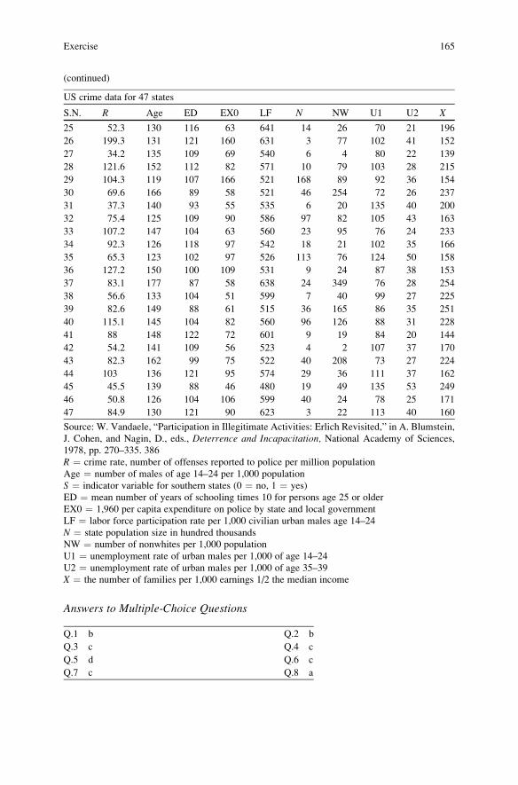
(continued)
US crime data for 47 states
S.N. R Age ED EX0 LF N NW U1 U2 X
25 52.3 130 116 63 641 14 26 70 21 196
26 199.3 131 121 160 631 3 77 102 41 152
27 34.2 135 109 69 540 6 4 80 22 139
28 121.6 152 112 82 571 10 79 103 28 215
29 104.3 119 107 166 521 168 89 92 36 154
30 69.6 166 89 58 521 46 254 72 26 237
31 37.3 140 93 55 535 6 20 135 40 200
32 75.4 125 109 90 586 97 82 105 43 163
33 107.2 147 104 63 560 23 95 76 24 233
34 92.3 126 118 97 542 18 21 102 35 166
35 65.3 123 102 97 526 113 76 124 50 158
36 127.2 150 100 109 531 9 24 87 38 153
37 83.1 177 87 58 638 24 349 76 28 254
38 56.6 133 104 51 599 7 40 99 27 225
39 82.6 149 88 61 515 36 165 86 35 251
40 115.1 145 104 82 560 96 126 88 31 228
41 88 148 122 72 601 9 19 84 20 144
42 54.2 141 109 56 523 4 2 107 37 170
43 82.3 162 99 75 522 40 208 73 27 224
44 103 136 121 95 574 29 36 111 37 162
45 45.5 139 88 46 480 19 49 135 53 249
46 50.8 126 104 106 599 40 24 78 25 171
47 84.9 130 121 90 623 3 22 113 40 160
Source: W. Vandaele, “Participation in Illegitimate Activities: Erlich Revisited,” in A. Blumstein,
J. Cohen, and Nagin, D., eds., Deterrence and Incapacitation, National Academy of Sciences,
1978, pp. 270–335. 386
R ¼ crime rate, number of offenses reported to police per million population
Age ¼ number of males of age 14–24 per 1,000 population
S ¼ indicator variable for southern states (0 ¼ no, 1 ¼ yes)
ED ¼ mean number of years of schooling times 10 for persons age 25 or older
EX0 ¼ 1,960 per capita expenditure on police by state and local government
LF ¼ labor force participation rate per 1,000 civilian urban males age 14–24
N ¼ state population size in hundred thousands
NW ¼ number of nonwhites per 1,000 population
U1 ¼ unemployment rate of urban males per 1,000 of age 14–24
U2 ¼ unemployment rate of urban males per 1,000 of age 35–39
X ¼ the number of families per 1,000 earnings 1/2 the median income
Answers to Multiple-Choice Questions
Q.1 b Q.2 b
Q.3 c Q.4 c
Q.5 d Q.6 c
Q.7 c Q.8 a
Exercise 165

Chapter 6
Hypothesis Testing for Decision-Making
Learning Objectives
After completing this chapter, you should be able to do the following:
• Understand the purpose of hypothesis testing.
• Learn to construct the hypotheses.
• Know the situations for using one- and two-tailed tests.
• Describe the procedure of hypothesis testing.
• Understand the p value.
• Learn the computing procedure manually in different situations by using t-tests.• Identify an appropriate t-test in different research situations.
• Know the assumptions under which t-test should be used.
• Describe the situations in which one-tailed and two-tailed tests should be used.
• Interpret the difference between one-tailed and two-tailed hypotheses.
• Learn to compute t-statistic in different research situations by using SPSS.
• Learn to interpret the outputs of different t-tests generated in SPSS.
Introduction
Human beings are progressive in nature. Most of our decisions in life are governed
by our past experiences. These decisions may be subjective or objective. Subjective
decisions are solely based upon one’s own perception of viewing issues. These
perceptions keep on changing from person to person. Same thing or situation can
be perceived differently by different persons, and therefore, the decision cannot be
universalized. On the other hand, if decisions are taken on the basis of scientific
law, it is widely accepted and works well in the similar situations.
Decision makers are always engaged in identifying optimum decision in a given
situation for solving a problem. Theory of statistical inference which is based on
scientific principles provide optimum solution to these decision makers. Statistical
inference includes theory of estimation and testing of hypothesis. In this chapter,
J.P. Verma, Data Analysis in Management with SPSS Software,DOI 10.1007/978-81-322-0786-3_6, # Springer India 2013
167

different aspects of hypothesis testing regarding population parameter have been
discussed. At times one may be interested to know as to whether the population
mean is equal to the given value. In testing such hypothesis, a representative sample
may be drawn to verify it by using statistical tests. Testing of hypothesis may be
done for comparing two population averages on the basis of samples drawn from
these populations. For instance, one may like to know whether memory retention
power is more in girls or in boys in a particular age category or whether motivation
level of employees in two different units of an organization is same or not. By
comparing sample means of two groups, we intend to find out whether these
samples come from the same population. In other words, we try to test whether
their population means are equal or not. In this chapter, procedure of hypothesis
testing in comparative studies has been discussed in detail. Besides comparative
studies, the researcher may be interested to see the effect of certain treatment on
dependent variable. Impact of advertisement campaign on the sale of a product,
effect of training on employee’s performance, and effect of stress management
program on absenteeism are such examples where the posttesting mean may be
compared with that of pretesting mean on the dependent variable.
For testing a hypothesis concerning mean, two statistical tests “t” and “z” are
normally used. In case of small sample, t-test is used, whereas z-test is used in large-sample case. For all practical purposes, a sample is considered to be small if its size
is less than or equal to 30 and large if it is more than 30. Since t-distributionapproaches to z-distribution for n > 30, t-test can be considered as a specific case ofz-test. The t-test is used in a situation where population is normally distributed and
population variance is not known, and on the other hand Z test is used when
population variance is known. In this chapter, only t-tests in different situations
have been discussed.
Usually testing of hypothesis is done for population mean and variance as these
are the two indices which are used to describe the nature of data to a great extent.
In this chapter, only testing of hypothesis concerning mean in different situations
has been discussed in great detail. Plan of choosing a statistical test for testing a
hypothesis has been shown graphically in Fig. 6.1.
This chapter describes the procedure of testing a hypothesis concerning single
group mean and the difference between two group means for unrelated and related
groups.
Hypothesis Construction
Hypotheses are any assertion or statement about certain characteristics of the
population. If the characteristics can be quantitatively measured by parameters
such as mean or variance, then the hypothesis based on these parameters is said
to be parametric. Whereas if the characteristics are qualitatively measured (e.g.,
assessment of quality, attitude, or perception), then the hypothesis so developed on
these characteristics is known as nonparametric hypothesis. These parametric and
168 6 Hypothesis Testing for Decision-Making

nonparametric hypotheses are known as statistical hypotheses. A hypothesis is said
to be statistical hypothesis if the following three conditions prevail:
1. The population may be defined.
2. Sample may be drawn.
3. The sample may be evaluated to test the hypothesis.
Statistical hypotheses are based on the concept of proof by contradiction. For
example, consider that a hypothesis concerning population mean (m) is tested to seeif an experiment has caused an increase or decrease in m. This is done by proof of
contradiction by formulating a null hypothesis. Thus, in testing of hypothesis, one
needs to formulate a research hypothesis which is required to be tested for some
Testing of Hypothesis
Hypothesis concerning mean Hypothesis concerning Variance
Population variances knownUse Z–test (N³30)
Population variances unknownUse t –test (N<30)
Test concerning two group means
Test concerning single group mean
Use Z-test forsingle group
Use Z-test for comparing two group means
Test concerning single group mean
Test concerning twogroup means
Use student’s t-testfor single group
Comparing two group means (Unrelated groups)
Comparing two group means (Related groups)
Use two sample t-test Use paired t-test Use F-test
n/
xz
s
m-=
2
22
1
21
21
nn
xxz
s+
s
-=
n/s
xt
m-=
21
21
n1
n1
S
xxt
+
-=
n/s
dt
d
= 22
21
S
SF=
Comparing group variances
Fig. 6.1 Scheme of selecting test statistic in hypothesis testing
Hypothesis Construction 169

population parameter. Based on research hypothesis, a null hypothesis is
formulated. The null and the research (alternative) hypotheses are complementary
to each other. In fact the null hypothesis serves as a means of testing the research
hypothesis, and therefore, rejection of null hypothesis allows the researcher to
accept the research hypothesis.
Null Hypothesis
Null hypothesis is a hypothesis of no difference. It is denoted by H0. It is formulated
to test an alternative hypothesis. Null hypothesis is assumed to be true. By assuming
the null hypothesis to be true, the distribution of the test statistic can be well
defined. Further, null signifies the unbiased approach of the researcher in testing
the research hypothesis. The researcher verifies the null hypothesis by assuming
that it is true and rejects it in favor of research hypothesis if any contradiction is
observed. In fact the null hypothesis is made for rejection. In case if the null
hypothesis cannot be rejected on the basis of the sample data, it is said that the
researcher fails to reject the null hypothesis. The sole purpose of the researcher is to
try rejecting the null hypothesis in favor of research hypothesis in case the contra-
diction is observed on the basis of the sample.
Alternative Hypothesis
Alternative hypothesis is also known as research hypothesis. In any research study,
the researcher first develops a research hypothesis for testing some parameter of the
population, and accordingly null hypothesis is formulated to verify it. The alterna-
tive hypothesis is denoted by H1. Alternative hypothesis means that there is a
difference between the population parameter and the sample value. In testing of
hypothesis, the whole focus is to test whether research hypothesis can be accepted
or not, and this is done by contradicting the null hypothesis.
Test Statistic
In hypothesis testing, the decision about rejecting or not rejecting the null hypothe-
sis depends upon the value of test statistic. A test statistic is a random variable
X whose value is tested against the critical value to arrive at a decision.
If a random sample of size n is drawn from the normal population with mean, mand variance, s2, then the sampling distribution of mean will also be normal with
mean m and variance s2/n. As per the central limit theorem even if the population
from which the sample is drawn is not normal, the sample mean will still follow the
normal distribution with mean, m, and variance s2/n provided the sample size n is
large (n > 30).
170 6 Hypothesis Testing for Decision-Making

Thus, in case of large sample (n > 30), for testing the hypothesis concerning
mean, z-test is used. However, in cases of small sample (n � 30), the distribution of
sample mean follows t-distribution if the population variance is not known. In suchsituation, t-test is used. In case population standard deviation (s) is unknown, it isestimated by the sample standard deviation(S). For different sample size, the
t-curve is different, and it approaches to normal curve for sample size n > 30.
All these curves are symmetrical and bell shaped and distributed around t ¼ 0. The
exact shape of the t-curve depends on the degrees of freedom.
In one-way ANOVA, the comparison between group variance and within-group
variance is done by using the F-statistic. The critical value of F can be obtained
from the Table A4 or A5 in appendix for a particular level of significance and the
degrees of freedom between and within the groups.
Rejection Region
Rejection region is a part of the sample space in which if the value of test statistic
falls, null hypothesis is rejected. Rejection region is also known as critical region. The
value of the statistic in the distribution that divides sample space into acceptance and
rejection region is known as critical value. These can be seen in Fig. 6.2.
The size of the rejection region is determined by the level of significance (a).The level of significance is that probability level below which we reject the null
hypothesis. The term statistical significance of a statistic refers only to the rejection
of a null hypothesis at some level a. It indicates that the observed difference
between the sample mean and the mean of the sampling distribution did not
occur by chance alone. So to conclude, if the test statistic falls in the rejection/
critical region, H0 is rejected, else H0 is failed to be rejected.
Steps in Hypothesis Testing
In experimental research, the inferences are drawn on the basis of testing a
hypothesis on population parameters. The following steps are involved in
decision-making process:
1. Formulate the null and alternative hypothesis for each of the parameters to be
investigated. It is important to mention as to whether the hypothesis required to
be tested is one tailed or two tailed.
2. Choose the level of significance at which the hypothesis needs to be tested.
Usually in experimental research, the significance levels are chosen as 0.01,
0.05, or 0.10, but any value between 0 and 1 can be used.
3. Identify the test statistic (follow the guidelines shown in Fig. 6.1) that can be used
to test the null hypothesis, and compute its value on the basis of the sample data.
4. Obtain the tabulated value of the statistic from the designated table. Care must be
taken to obtain its value as its values are different at the same level of signifi-
cance for one-tailed and two-tailed hypotheses.
Steps in Hypothesis Testing 171
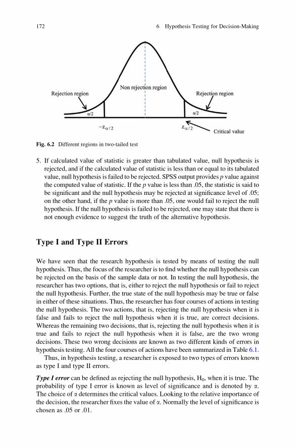
5. If calculated value of statistic is greater than tabulated value, null hypothesis is
rejected, and if the calculated value of statistic is less than or equal to its tabulated
value, null hypothesis is failed to be rejected. SPSS output provides p value againstthe computed value of statistic. If the p value is less than .05, the statistic is said tobe significant and the null hypothesis may be rejected at significance level of .05;
on the other hand, if the p value is more than .05, one would fail to reject the null
hypothesis. If the null hypothesis is failed to be rejected, one may state that there is
not enough evidence to suggest the truth of the alternative hypothesis.
Type I and Type II Errors
We have seen that the research hypothesis is tested by means of testing the null
hypothesis. Thus, the focus of the researcher is to find whether the null hypothesis can
be rejected on the basis of the sample data or not. In testing the null hypothesis, the
researcher has two options, that is, either to reject the null hypothesis or fail to reject
the null hypothesis. Further, the true state of the null hypothesis may be true or false
in either of these situations. Thus, the researcher has four courses of actions in testing
the null hypothesis. The two actions, that is, rejecting the null hypothesis when it is
false and fails to reject the null hypothesis when it is true, are correct decisions.
Whereas the remaining two decisions, that is, rejecting the null hypothesis when it is
true and fails to reject the null hypothesis when it is false, are the two wrong
decisions. These two wrong decisions are known as two different kinds of errors in
hypothesis testing. All the four courses of actions have been summarized in Table 6.1.
Thus, in hypothesis testing, a researcher is exposed to two types of errors known
as type I and type II errors.
Type I error can be defined as rejecting the null hypothesis, H0, when it is true. The
probability of type I error is known as level of significance and is denoted by a.The choice of a determines the critical values. Looking to the relative importance of
the decision, the researcher fixes the value of a. Normally the level of significance is
chosen as .05 or .01.
Fig. 6.2 Different regions in two-tailed test
172 6 Hypothesis Testing for Decision-Making
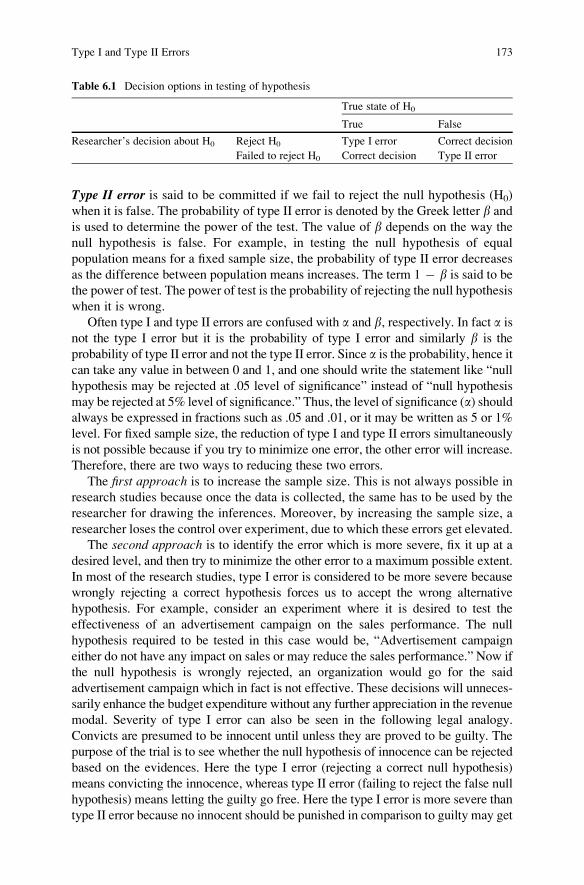
Type II error is said to be committed if we fail to reject the null hypothesis (H0)
when it is false. The probability of type II error is denoted by the Greek letter b and
is used to determine the power of the test. The value of b depends on the way the
null hypothesis is false. For example, in testing the null hypothesis of equal
population means for a fixed sample size, the probability of type II error decreases
as the difference between population means increases. The term 1 � b is said to be
the power of test. The power of test is the probability of rejecting the null hypothesis
when it is wrong.
Often type I and type II errors are confused with a and b, respectively. In fact a isnot the type I error but it is the probability of type I error and similarly b is the
probability of type II error and not the type II error. Since a is the probability, hence itcan take any value in between 0 and 1, and one should write the statement like “null
hypothesis may be rejected at .05 level of significance” instead of “null hypothesis
may be rejected at 5% level of significance.” Thus, the level of significance (a) shouldalways be expressed in fractions such as .05 and .01, or it may be written as 5 or 1%
level. For fixed sample size, the reduction of type I and type II errors simultaneously
is not possible because if you try to minimize one error, the other error will increase.
Therefore, there are two ways to reducing these two errors.
The first approach is to increase the sample size. This is not always possible in
research studies because once the data is collected, the same has to be used by the
researcher for drawing the inferences. Moreover, by increasing the sample size, a
researcher loses the control over experiment, due to which these errors get elevated.
The second approach is to identify the error which is more severe, fix it up at a
desired level, and then try to minimize the other error to a maximum possible extent.
In most of the research studies, type I error is considered to be more severe because
wrongly rejecting a correct hypothesis forces us to accept the wrong alternative
hypothesis. For example, consider an experiment where it is desired to test the
effectiveness of an advertisement campaign on the sales performance. The null
hypothesis required to be tested in this case would be, “Advertisement campaign
either do not have any impact on sales or may reduce the sales performance.” Now if
the null hypothesis is wrongly rejected, an organization would go for the said
advertisement campaign which in fact is not effective. These decisions will unneces-
sarily enhance the budget expenditure without any further appreciation in the revenue
modal. Severity of type I error can also be seen in the following legal analogy.
Convicts are presumed to be innocent until unless they are proved to be guilty. The
purpose of the trial is to see whether the null hypothesis of innocence can be rejected
based on the evidences. Here the type I error (rejecting a correct null hypothesis)
means convicting the innocence, whereas type II error (failing to reject the false null
hypothesis) means letting the guilty go free. Here the type I error is more severe than
type II error because no innocent should be punished in comparison to guilty may get
Table 6.1 Decision options in testing of hypothesis
True state of H0
True False
Researcher’s decision about H0 Reject H0 Type I error Correct decision
Failed to reject H0 Correct decision Type II error
Type I and Type II Errors 173
no punishment. Type I error becomes more serious if the crime is murder and the
person gets the punishment of death sentence. Thus, usually in research studies, the
type I error is fixed at the desired level of, say, .05 or .01 and then type II error is tried
to be minimized as much as possible.
The value of a and b depends upon each other. For a fixed sample size, the only
way to reduce the probability of making one type of error is to increase the other.
Consider a situation where it is desired to compare the means of two populations.
Let us assume that the rejection regions have critical values�1. Using the statistical
test, H0 will never get rejected as it will exclude every possible difference in sample
means. Since the null hypothesis will never be rejected, the probability of rejecting
the null hypothesis when it is true will be zero. In other words, the value of a ¼ 0.
Since the null hypothesis will never be rejected, the probability of type II error
(failing to reject the null hypothesis when it is false) will be 1 or to say that b ¼ 1.
Now consider the rejection regions whose critical values are 0,0. In this case, the
rejection region includes every possible difference in sample means. This test will
always reject H0. Since the null hypothesis will always be rejected, the probability
of type I error (rejecting H0 when it is true) will be 1 or the value of a ¼ 1. Since the
null hypothesis is always rejected, the probability of type II error (failing to reject
H0 when it is false) is 0, or the value of b ¼ 0.
To conclude, a statistical test having rejection region bounded by the critical
values �1 has a ¼ 0 and b ¼ 1, whereas the test with a rejection region bounded
by the critical values 0,0 has a ¼ 1 and b ¼ 0. Consider a test having rejection
region bounded by the critical values� q. As q increases from 0 to1, a decreases
from 1 to 0, while b increases from 0 to 1.
One-Tailed and Two-Tailed Tests
Consider an experiment in which null and alternative hypotheses are H0 and H1,
respectively. We perform a test to determine whether or not the null hypothesis
should be rejected in favor of the alternative hypothesis. In this situation, two
different kinds of tests can be performed. One may either use a one-tailed test tosee whether there is an increase or decrease in the parameter or may decide to use a
two-tailed test to verify for any change in the parameter that can be increased or
decrease. The word tail refers to the far left and far right of a distribution curve.
These one-tailed and two-tailed tests can be performed at any of the two, 0.01 or
0.05, levels of significance.
One-Tailed Test A statistical test is known as one-tailed test if the null hypothesis
(H0) is rejected only for the values of the test statistic falling into one specified tail of
its sampling distribution. In one-tailed test, the direction is specified, that is, we are
interested to verify whether population parameter is greater than some value. Or at
times we may be interested to know whether the population parameter is less than
some value. In other words, the researcher is clear as to what specifically he/she is
interested to test. Depending upon the research hypothesis, one-tailed test can be
classified as right-tailed or left-tailed tests. If the research hypothesis is to test whether
174 6 Hypothesis Testing for Decision-Making

the population mean is greater than some specified value, then the test is known as
right-tailed test and the entire critical region shall lie in the right tail only. And if the
test statistic falls into right critical region, the alternative hypothesis will be accepted
instead of the null hypothesis. On the other hand, if the research hypothesis is to test
whether the population mean is less than some specified value, then the test is known
as left-tailed test and the entire critical region shall lie in the left tail only. The critical
regions at 5% level in both these situations are shown in Fig. 6.3.
Two-Tailed Test A statistical test is said to be a two-tailed test if the null
hypothesis (H0) is rejected only for values of the test statistic falling into either
tail of its sampling distribution. In two-tailed test, no direction is specified. We are
only interested to test whether the population parameter is either greater than or less
than some specified value. If the test statistic falls into either of the critical regions,
the alternative hypothesis will be accepted instead of the null hypothesis. In two-
tailed test, the critical region is divided in both the tails. For example, if the null
hypothesis is tested at 5% level, the critical region shall be divided in both the tails
as shown in Fig. 6.4. Tables A.1 and A.2 in Appendix provide critical values for z-test and t-test, respectively.
Criteria for Using One-Tailed and Two-Tailed Tests
A one-tailed test is usedwhenwe are quite sure about the direction of the difference in
advance (e.g., exercise will improve the fitness level). With that assumption, the level
of significance (a) is only calculated from one tail of the distribution. However, in
standard testing, the probability is calculated from both tails.
Fig. 6.3 Critical regions at 5% level in (a) left-tailed test and (b) right-tailed test
0.025
−Zα/2 = −1.96 Zα/2 = 1.96
0.025
Fig. 6.4 Critical regions in
two-tailed tests
Criteria for Using One-Tailed and Two-Tailed Tests 175

For instance if the significance of correlation is tested between age and medical
expenses; onemight hypothesize thatmedical expensesmay increase or do not increase
but will never decrease with age. In such case one-tailed hypothesis should be used.
On the other hand, in testing the correlation between people’s weights with their
income, wemay not have reasons to believe that the incomewill increase with increase
in weights or the income will decreases with weights. Here we might be interested just
to find out if there was any relationship at all and that is a two-tailed hypothesis.
The issue in deciding between one-tailed and two-tailed tests is not whether or
not you expect a difference to exist. Had you known whether or not there was a
difference, there is no reason to collect the data. Instead, the question is whether the
direction of a difference can only go one way. One should only use a one-tailed test
if there is an absolute certainty before data collection that in the overall populations,
either there is no difference or there is a difference in a specified direction. Further,
if you end up showing a difference in the opposite direction, you should be ready to
attribute that difference to random sampling without bothering about the fact that
the measured difference might reflect a true difference in the overall populations.
If a difference in the “wrong” direction brings even little meaning to your findings,
you should use two-tailed test.
The advantage of using one-tailed hypothesis is that you can use a smaller
sample to test it. The smaller sample often reduces your cost of the experiment.
But on the other hand, it is easier to reject the null hypothesis with a one-tailed test
in comparison to two-tailed test. Thus, the level of significance increases in one-
tailed test. Because of this reason, it is rarely correct to perform a one-tailed test;
usually we want to test whether any difference exists.
Strategy in Testing One-Tailed and Two-Tailed Tests
The strategy in choosing between one-tailed and two-tailed tests is to prefer a two-
tailed test unless there is a strong belief that the difference in the population can
only be in one direction. If the two-tailed test is statistically significant (p < a),interpret the findings in one-tailed manner. Consider an experiment in which it is
desired to test the null hypothesis that the average cure time of cold and cough by a
newly introduced vitamin C tablet is 4 days against an alternative hypothesis that it
is not. If a sample of 64 patients has an average recovery time of 3.5 days with
s ¼ 1.0 day, the p value in this testing would be 0.0002 and therefore the null
hypothesis H0 will be rejected and we accept the alternative hypothesis H1. Thus, in
this situation, it is concluded that the recovery time is not equal to 4 days for the
new prescription of vitamin C.
But we may conclude more than that in saying that the recovery time is less than
4 days with the new prescription of vitamin C. We arrive at this conclusion by
combining the two facts: Firstly, we have proved that the recovery time is different
than 4 days, which means it must be either less or more than 4 days, and secondly,
the sample mean �X (¼3.5 days) in this problem is less than the specified value, that
176 6 Hypothesis Testing for Decision-Making

is, 4 days(population mean). After combining these two facts, it may be concluded
that the average recovery time (3.5 days) is significantly lower than the 4 days. This
conclusion is quite logical because if we again test the null hypothesis H0:m � 4
against the alternative hypothesis H1:m < 4(one-tailed test), the p value would be
0.0001 which is even smaller than 0.0002.
Thus, we may conclude first by answering the original question then going for
writing about the directional difference such as “The mean recovery time in cold and
cough symptom with the new prescription of vitamin C is different from 4 days”; in
fact, it is less than 4 days.
What Is p Value?
The p value is the probability of wrongly rejecting the null hypothesis. It is
analogous to the level of significance. Usually an experimenter decides to test the
hypothesis at some desired level of significance. If the absolute value of test statistic
increases, the probability of rejecting the correct null hypothesis decreases. Thus, if
a null hypothesis is tested at the level of significance .05 and the value of test
statistic is large so that its corresponding p value is 0.004, in that case if we
conclude that the null hypothesis is rejected at 5% level, it would not be logically
correct as the error attached to this judgment is only 0.4%. In fact as the absolute
value of test statistic increases, the p value keeps on decreasing.
One may decide the level of significance in advance say, 0.05, but while
explaining the decision, the concept of p value should be used to report as to how
much error is involved in the decision about rejecting or being unable to reject the
null hypothesis. Thus, while testing a hypothesis, a p value is calculated against the
test statistic which is used to explain the error involved in the decision. In SPSS and
other statistical packages, the p values are automatically computed against each test
statistic. Thus, if an experimenter decides to test the hypothesis at the significance
level of 0.05, the test statistic shall be significant so long p value is less than 0.05. Thegeneral practice is to write the p value along with the value of test statistic. For
instance, we may write as “Since the calculated t ¼ 4.0(p ¼ 0.0002) is significant,
the null hypothesis may be rejected.” The p value may be calculated against the value
of t-statistic by using the t-table or by using the free conversion software available onmany sites such as http://faculty.vassar.edu/lowry/tabs.html#t.
Degrees of Freedom
Any parameter can be estimated with certain amount of information or data set. The
number of independent pieces of data or scores that are used to estimate a parameter is
known as degrees of freedom and is usually abbreviated as df. In general, the degrees
of freedom of an estimate are calculated as the number of independent scores that are
required to estimate the parameter minus the number of parameters estimated as
Degrees of Freedom 177
intermediate steps in the estimation of the parameter itself. In general, each item being
estimated costs one degree of freedom.
The degrees of freedom can be defined as the number of independent scores or
pieces of information that are free to vary in computing a statistic.
Since the variance s2 is estimated by the statistic S2 which is computed from a
random sample of n independent scores, let us see what the degrees of freedom of S2
are. Since S is computed from the sample of n scores, its degrees of freedom would
have been n, but because one degree of freedom is lost due to the condition thatPX � �Xð Þ ¼ 0, the degrees of freedom for S2 are n � 1. If we go by the definition,
the degrees of freedom of S2 are equal to the number of independent scores (n)minus the number of parameters estimated as intermediate steps (one, as m is
estimated by �X) and are therefore equal to n � 1.
In case of two samples, pooled standard deviation S is computed by using
n1 + n2 observations. In the computation of S, the two parameters m1 and m2 are
estimated by �X1, and �X2 hence, the two degrees of freedom are lost and therefore the
degrees of freedom for estimating S are n1 + n2 � 2.
In computing chi-square in a 2 � 2 contingency table for testing the indepen-
dence between rows and columns, it is assumed that you already know 3 pieces of
information: the row proportions, the column proportions, and the total number of
observations. Since the total number of pieces of information in the contingency
table is 4, and 3 are already known before computing the chi-square statistic, the
degrees of freedom are 4 � 3 ¼ 1. We know that the degrees of freedom for chi-
square are obtained by (r � 1) � (c � 1); hence, with this formula, also the
degrees of freedom in a 2 � 2 contingency table are 1.
One-Sample t-Test
A t-test can be defined as a statistical test used for testing of hypothesis in which the
test statistic follows a Student’s t-distribution under the assumption that the null
hypothesis is true. This test is used if the population standard deviation is not known
and the distribution of the population from which the sample has been drawn is
normally distributed. Usually t-test is used for small sample size (n < 30) in a
situation where population standard deviation is not known. Even if the sample is
large (n � 30) but if the population standard deviation is not known in that situation,
also t-test should be used instead of z-test. A one-sample t-test is used for testing
whether the population mean is equal to a predefined value or not. An example of a
one-sample t-test may be to see whether population average sleep time is equal to 5 h
or not.
In using t-test, it is assumed that the distribution of data is approximately normal.
The t-distribution depends on the sample size. Its parameter is called the degrees of
freedom (df) which is equal to n � 1, where n is the sample size.
178 6 Hypothesis Testing for Decision-Making
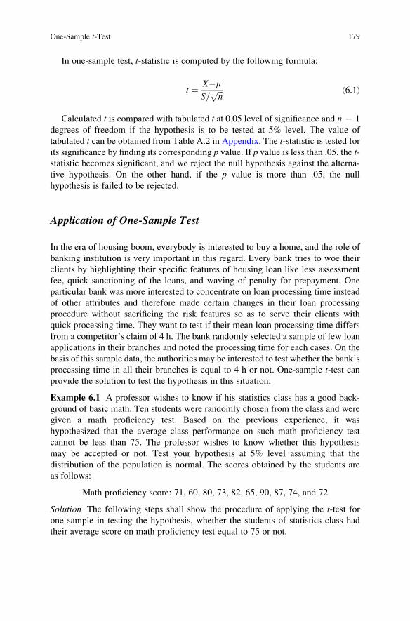
In one-sample test, t-statistic is computed by the following formula:
t ¼�X�mS=
ffiffiffin
p (6.1)
Calculated t is compared with tabulated t at 0.05 level of significance and n � 1
degrees of freedom if the hypothesis is to be tested at 5% level. The value of
tabulated t can be obtained from Table A.2 in Appendix. The t-statistic is tested forits significance by finding its corresponding p value. If p value is less than .05, the t-statistic becomes significant, and we reject the null hypothesis against the alterna-
tive hypothesis. On the other hand, if the p value is more than .05, the null
hypothesis is failed to be rejected.
Application of One-Sample Test
In the era of housing boom, everybody is interested to buy a home, and the role of
banking institution is very important in this regard. Every bank tries to woe their
clients by highlighting their specific features of housing loan like less assessment
fee, quick sanctioning of the loans, and waving of penalty for prepayment. One
particular bank was more interested to concentrate on loan processing time instead
of other attributes and therefore made certain changes in their loan processing
procedure without sacrificing the risk features so as to serve their clients with
quick processing time. They want to test if their mean loan processing time differs
from a competitor’s claim of 4 h. The bank randomly selected a sample of few loan
applications in their branches and noted the processing time for each cases. On the
basis of this sample data, the authorities may be interested to test whether the bank’s
processing time in all their branches is equal to 4 h or not. One-sample t-test canprovide the solution to test the hypothesis in this situation.
Example 6.1 A professor wishes to know if his statistics class has a good back-
ground of basic math. Ten students were randomly chosen from the class and were
given a math proficiency test. Based on the previous experience, it was
hypothesized that the average class performance on such math proficiency test
cannot be less than 75. The professor wishes to know whether this hypothesis
may be accepted or not. Test your hypothesis at 5% level assuming that the
distribution of the population is normal. The scores obtained by the students are
as follows:
Math proficiency score: 71, 60, 80, 73, 82, 65, 90, 87, 74, and 72
Solution The following steps shall show the procedure of applying the t-test forone sample in testing the hypothesis, whether the students of statistics class had
their average score on math proficiency test equal to 75 or not.
One-Sample t-Test 179
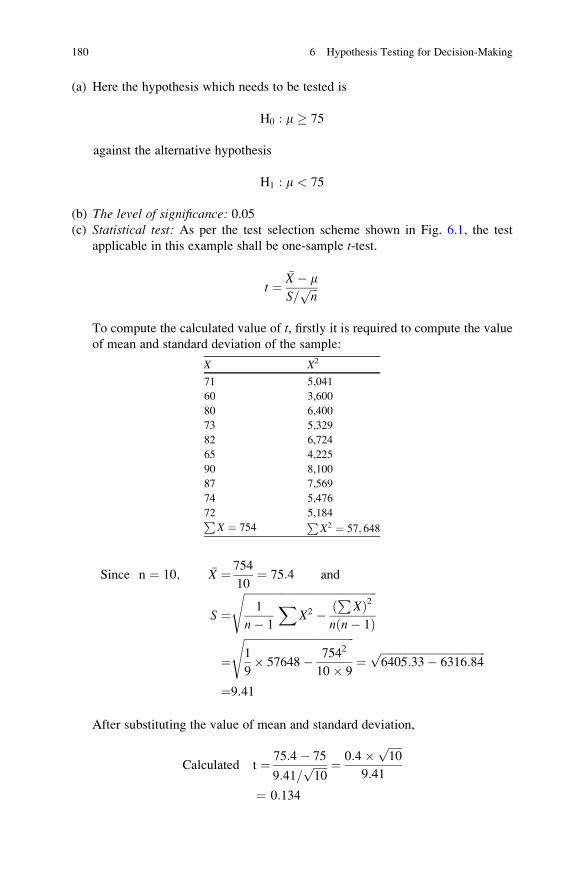
(a) Here the hypothesis which needs to be tested is
H0 : m � 75
against the alternative hypothesis
H1 : m < 75
(b) The level of significance: 0.05(c) Statistical test: As per the test selection scheme shown in Fig. 6.1, the test
applicable in this example shall be one-sample t-test.
t ¼�X � mS=
ffiffiffin
p
To compute the calculated value of t, firstly it is required to compute the value
of mean and standard deviation of the sample:
X X2
71 5,041
60 3,600
80 6,400
73 5,329
82 6,724
65 4,225
90 8,100
87 7,569
74 5,476
72 5,184PX ¼ 754
PX2 ¼ 57; 648
Since n ¼ 10; �X ¼ 754
10¼ 75:4 and
S ¼ffiffiffiffiffiffiffiffiffiffiffiffiffiffiffiffiffiffiffiffiffiffiffiffiffiffiffiffiffiffiffiffiffiffiffiffiffiffiffiffiffiffiffiffiffiffiffiffi1
n� 1
XX2 �
PXð Þ2
nðn� 1Þ
s
¼ffiffiffiffiffiffiffiffiffiffiffiffiffiffiffiffiffiffiffiffiffiffiffiffiffiffiffiffiffiffiffiffiffiffiffiffiffiffiffiffi1
9� 57648� 7542
10� 9
s¼
ffiffiffiffiffiffiffiffiffiffiffiffiffiffiffiffiffiffiffiffiffiffiffiffiffiffiffiffiffiffiffiffiffiffiffiffiffiffi6405:33� 6316:84
p
¼9:41
After substituting the value of mean and standard deviation,
Calculated t ¼ 75:4� 75
9:41=ffiffiffiffiffi10
p ¼ 0:4� ffiffiffiffiffi10
p
9:41
¼ 0:134
180 6 Hypothesis Testing for Decision-Making

(d) Decision criteria: From Table A.2 in Appendix, the tabulated value of t for one-tailed test at .05 level of significance with 9 degrees of freedom is
t:05ð9Þ ¼ 1:833:Since calculated t ¼ 0:134ð Þ<t:05ð9Þ, hence the null hypothesis is failed to be
rejected at 5% level.
(e) Inference: Since the null hypothesis is failed to be rejected, hence the alterna-
tive hypothesis that the average math proficiency performance of the students is
less than 75 cannot be accepted. Thus, it may be concluded that the average
students’ performance on math proficiency test is equal or higher than 75.
Two-Sample t-Test for Unrelated Groups
The two-sample t-test is used for testing the hypothesis of equality of means of two
normally distributed populations. All t-tests are usually called Student’s t-tests. Butstrictly speaking, this name should be used only if the variances of the two
populations are also assumed to be equal. Two-sample t-test is based on the
assumption that the variances of the populations s21 and s22 are unknown and
population distributions are normal. In case the assumptions of equality of
variances are not met, then the test used in such situation is called as Welch’s t-test. Readers may read some other text for this test.
We often want to compare the means of two different populations, for example,
comparing the effect of two different diets on weights, the effect of two teaching
methodologies on the performance, or the IQ of boys and girls. In such situations,
two-sample t-test can be used. One of the conditions of using two-sample t-test isthat the samples are independent and identically distributed. Consider an experi-
ment in which the job satisfaction needs to be compared among the bank employees
working in rural and urban areas. Two randomly selected groups of 30 subjects each
may be selected from rural and urban areas. Assuming all other conditions of the
employees like salary structure, status and age categories to be similar, null
hypothesis of no difference in their job satisfaction scores may be tested by using
the two-sample t-test for independent samples. In this case, the two samples are
independent because subjects in both the groups are not same.
Assumptions in Using Two-Sample t-Test
The following assumptions need to be fulfilled before using the two-sample t-testfor independent groups:
• The distributions of both the populations from which the samples have been
drawn are normally distributed.
• The variances of the two populations are nearly equal.
Two-Sample t-Test for Unrelated Groups 181

• Population variances are unknown.
• The samples are independent to each other.
Since we assume that s21 and s22 are equal, we can compute a pooled variance S2
of both the samples. The purpose of pooling the variances is to obtain a better
estimate. The pooled variance is a weighted sum of variances. Thus, if the sample
sizes n1 and n2 are equal, then S2 is just an average of the individual variances. The
overall degrees of freedom in that case will be the sum of the individual degrees of
freedom of the two samples, that is,
df ¼ df þ df2 ¼ n1 � 1ð Þ þ n2 � 1ð Þ ¼ n1 þ n2 � 2
Computation of t-statistic is same irrespective of testing two-tailed or one-tailed
hypotheses. The only difference in testing these hypotheses are in its testing criteria
and critical values of “t.” These cases shall be discussed in the following sections.
Application of Two-Sampled t-Test
The situation where two-sample t-test is applicable can be easily understood by
looking to the following case study. A pharmaceutical company decided to conduct
an experiment to know as to whether high-protein diet or low-protein diets are more
responsible in increasing the weights of male mouse in a controlled environment.
Two groups of male mouse of similar age and weights may be selected randomly to
serve as the two experimental groups. The number of mouse may be equal or
unequal in both the groups. The first group may be fed with low-protein diet,
whereas the other may be on the high-protein diet. To compare the average increase
in their weights, two-sample t-test may be used to answer the research question.
Since one of the conditions of using the two-sample t-test is that the variance ofthe two groups must be equal, therefore F-test may be used to compare the
variability. Only if the variability of the two groups is equal the two-sample t-testshould be used. Here the null hypothesis of no difference in the increased weights of
the high and low-protein groups is tested against the alternative hypothesis that the
difference exists. In case the two-sample t-statistic is significant at some specified
level of significance, the null hypothesis may be rejected, and it may be concluded
that the effect of low-protein and high-protein diets on weights is different. On the
other hand, if the t-statistic is not significant, we failed to reject the null hypothesis,and it may be concluded that it is not possible to find any significant difference in
the rats’ weight kept on high- and low-protein diets.
Further, if the null hypothesis is rejected, the mean weight of the high- and low-
protein groups is seen, and if the average weight of the high-protein group is higher
than that of the low-protein group, it may be concluded that the high-protein diet is
more effective than the low-protein diet in increasing the weights of the rats.
182 6 Hypothesis Testing for Decision-Making
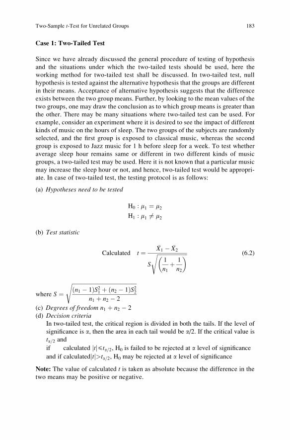
Case 1: Two-Tailed Test
Since we have already discussed the general procedure of testing of hypothesis
and the situations under which the two-tailed tests should be used, here the
working method for two-tailed test shall be discussed. In two-tailed test, null
hypothesis is tested against the alternative hypothesis that the groups are different
in their means. Acceptance of alternative hypothesis suggests that the difference
exists between the two group means. Further, by looking to the mean values of the
two groups, one may draw the conclusion as to which group means is greater than
the other. There may be many situations where two-tailed test can be used. For
example, consider an experiment where it is desired to see the impact of different
kinds of music on the hours of sleep. The two groups of the subjects are randomly
selected, and the first group is exposed to classical music, whereas the second
group is exposed to Jazz music for 1 h before sleep for a week. To test whether
average sleep hour remains same or different in two different kinds of music
groups, a two-tailed test may be used. Here it is not known that a particular music
may increase the sleep hour or not, and hence, two-tailed test would be appropri-
ate. In case of two-tailed test, the testing protocol is as follows:
(a) Hypotheses need to be tested
H0 : m1 ¼ m2H1 : m1 6¼ m2
(b) Test statistic
Calculated t ¼�X1 � �X2
S
ffiffiffiffiffiffiffiffiffiffiffiffiffiffiffiffiffiffiffiffiffiffi1
n1þ 1
n2
� �s (6.2)
where S ¼ffiffiffiffiffiffiffiffiffiffiffiffiffiffiffiffiffiffiffiffiffiffiffiffiffiffiffiffiffiffiffiffiffiffiffiffiffiffiffiffiffiffiffiffiffiffiffiðn1 � 1ÞS21 þ ðn2 � 1ÞS22
n1 þ n2 � 2
s
(c) Degrees of freedom n1 þ n2 � 2
(d) Decision criteriaIn two-tailed test, the critical region is divided in both the tails. If the level of
significance is a, then the area in each tail would be a/2. If the critical value ista=2 and
if calculated tj jbta=2, H0 is failed to be rejected at a level of significance
and if calculated tj j>ta=2, H0 may be rejected at a level of significance
Note: The value of calculated t is taken as absolute because the difference in the
two means may be positive or negative.
Two-Sample t-Test for Unrelated Groups 183

Case II: Right-Tailed Test (One-Tailed Test)
We have already discussed the situations in which one-tailed test should be used.
One-tailed test should only be used if an experimenter, on the basis of past
information, is absolutely sure that the difference can go only in one direction.
One-tailed test can be either right tailed or left tailed. In right-tailed test, it is desired
to test the hypothesis, whether mean of first group is greater than that of the mean of
the second group. In other words, the researcher is interested in a particular group
only. In such testing, if the null hypothesis is rejected, it can be concluded that the
first group mean is significantly higher than that of the second group mean. The
situation where right-tailed test can be used is to test whether frustration level is less
among those employees whose jobs are linked with incentives in comparison to
those whose jobs are not linked with the incentives. Here the first group is the one
whose jobs are linked with the incentives, whereas the second group’s jobs are not
linked with the incentives. In this situation, it is assumed that the employees feel
happy in their jobs if it is linked with incentives. The testing protocol in testing the
right-tailed hypothesis is as follows:
(a) Hypotheses need to be tested
H0 : m1bm2H1 : m1>m2
(b) Test statistic
Calculated t ¼�X1 � �X2
S
ffiffiffiffiffiffiffiffiffiffiffiffiffiffiffiffiffiffiffiffiffiffi1
n1þ 1
n2
� �s
where S ¼ffiffiffiffiffiffiffiffiffiffiffiffiffiffiffiffiffiffiffiffiffiffiffiffiffiffiffiffiffiffiffiffiffiffiffiffiffiffiffiffiffiffiffiffiffiffiffin1 � 1ð ÞS21 þ n2 � 1ð ÞS22
n1 þ n2 � 2
s
(c) Degrees of freedom n1 þ n2 � 2
(d) Decision criteriaIn one-tailed test, the entire critical region lies in one tail only. Here the
research hypothesis is the right tailed; hence, the entire critical region would
lie in the right tail only, and therefore, the sign of the critical value would be
positive. If the critical value is represented by ta andif calculated tbta, H0 is failed to be rejected at a level of significance
and if calculated t>ta, H0 may be rejected at a level of significance
Case III: Left-Tailed Test (One-Tailed Test)
At times the researcher is interested in testing whether a particular group mean is less
than the second one. In this type of hypothesis testing, it is desired to test whether
mean of first group is less than that of mean of the second group. Here if the null
184 6 Hypothesis Testing for Decision-Making
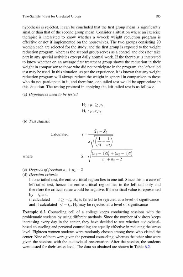
hypothesis is rejected, it can be concluded that the first group mean is significantly
smaller than that of the second group mean. Consider a situation where an exercise
therapist is interested to know whether a 4-week weight reduction program is
effective or not if implemented on the housewives. The two groups consisting 20
women each are selected for the study, and the first group is exposed to the weight
reduction program, whereas the second group serves as a control and does not take
part in any special activities except daily normal work. If the therapist is interested
to know whether on an average first treatment group shows the reduction in their
weight in comparison to those who did not participate in the program, the left-tailed
test may be used. In this situation, as per the experience, it is known that any weight
reduction program will always reduce the weight in general in comparison to those
who do not participate in it, and therefore, one tailed test would be appropriate in
this situation. The testing protocol in applying the left-tailed test is as follows:
(a) Hypotheses need to be tested
H0 : m1 � m2H1 : m1<m2
(b) Test statistic
Calculated t ¼�X1 � �X2
S
ffiffiffiffiffiffiffiffiffiffiffiffiffiffiffiffiffiffiffiffiffiffi1
n1þ 1
n2
� �s
where S ¼ffiffiffiffiffiffiffiffiffiffiffiffiffiffiffiffiffiffiffiffiffiffiffiffiffiffiffiffiffiffiffiffiffiffiffiffiffiffiffiffiffiffiffiffiffiffiffin1 � 1ð ÞS21 þ n2 � 1ð ÞS22
n1 þ n2 � 2
s
(c) Degrees of freedom n1 þ n2 � 2
(d) Decision criteriaIn one-tailed test, the entire critical region lies in one tail. Since this is a case of
left-tailed test, hence the entire critical region lies in the left tail only and
therefore the critical value would be negative. If the critical value is represented
by �ta andif calculated t � �ta, H0 is failed to be rejected at a level of significance
and if calculated <� ta, H0 may be rejected at a level of significance
Example 6.2 Counseling cell of a college keeps conducting sessions with the
problematic students by using different methods. Since the number of visitors keeps
increasing every day in the center, they have decided to test whether audiovisual-
based counseling and personal counseling are equally effective in reducing the stress
level. Eighteen women students were randomly chosen among those who visited the
center. Nine of them were given the personal counseling, whereas the other nine were
given the sessions with the audiovisual presentation. After the session, the students
were tested for their stress level. The data so obtained are shown in Table 6.2.
Two-Sample t-Test for Unrelated Groups 185
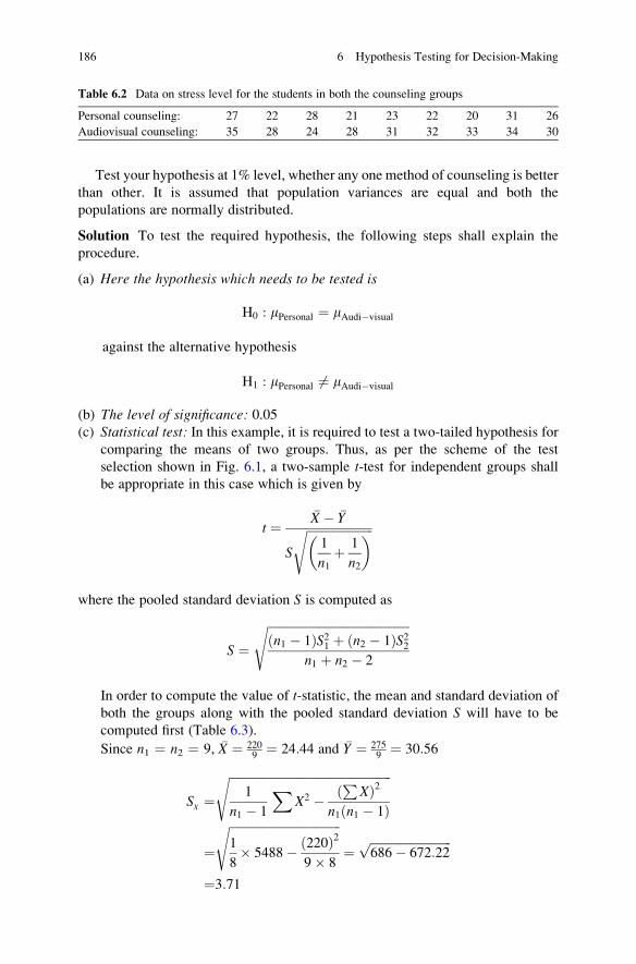
Test your hypothesis at 1% level, whether any one method of counseling is better
than other. It is assumed that population variances are equal and both the
populations are normally distributed.
Solution To test the required hypothesis, the following steps shall explain the
procedure.
(a) Here the hypothesis which needs to be tested is
H0 : mPersonal ¼ mAudi�visual
against the alternative hypothesis
H1 : mPersonal 6¼ mAudi�visual
(b) The level of significance: 0.05(c) Statistical test: In this example, it is required to test a two-tailed hypothesis for
comparing the means of two groups. Thus, as per the scheme of the test
selection shown in Fig. 6.1, a two-sample t-test for independent groups shallbe appropriate in this case which is given by
t ¼�X � �Y
S
ffiffiffiffiffiffiffiffiffiffiffiffiffiffiffiffiffiffiffiffiffiffi1
n1þ 1
n2
� �s
where the pooled standard deviation S is computed as
S ¼ffiffiffiffiffiffiffiffiffiffiffiffiffiffiffiffiffiffiffiffiffiffiffiffiffiffiffiffiffiffiffiffiffiffiffiffiffiffiffiffiffiffiffiffiffiffiffin1 � 1ð ÞS21 þ n2 � 1ð ÞS22
n1 þ n2 � 2
s
In order to compute the value of t-statistic, the mean and standard deviation of
both the groups along with the pooled standard deviation S will have to be
computed first (Table 6.3).
Since n1 ¼ n2 ¼ 9, �X ¼ 2209¼ 24:44 and �Y ¼ 275
9¼ 30:56
SX¼
ffiffiffiffiffiffiffiffiffiffiffiffiffiffiffiffiffiffiffiffiffiffiffiffiffiffiffiffiffiffiffiffiffiffiffiffiffiffiffiffiffiffiffiffiffiffiffiffiffiffiffiffiffiffi1
n1 � 1
XX2 �
PXð Þ2
n1 n1 � 1ð Þ
s
¼ffiffiffiffiffiffiffiffiffiffiffiffiffiffiffiffiffiffiffiffiffiffiffiffiffiffiffiffiffiffiffiffiffiffiffiffiffi1
8� 5488� 220ð Þ2
9� 8
s¼
ffiffiffiffiffiffiffiffiffiffiffiffiffiffiffiffiffiffiffiffiffiffiffiffiffiffiffi686� 672:22
p
¼3:71
Table 6.2 Data on stress level for the students in both the counseling groups
Personal counseling: 27 22 28 21 23 22 20 31 26
Audiovisual counseling: 35 28 24 28 31 32 33 34 30
186 6 Hypothesis Testing for Decision-Making

Similarly
SY¼
ffiffiffiffiffiffiffiffiffiffiffiffiffiffiffiffiffiffiffiffiffiffiffiffiffiffiffiffiffiffiffiffiffiffiffiffiffiffiffiffiffiffiffiffiffiffiffiffiffiffiffiffiffiffi1
n2 � 1
XY2 �
PYð Þ2
n2 n2 � 1ð Þ
s
¼ffiffiffiffiffiffiffiffiffiffiffiffiffiffiffiffiffiffiffiffiffiffiffiffiffiffiffiffiffiffiffiffiffiffiffiffiffi1
8� 8499� 275ð Þ2
9� 8
s¼
ffiffiffiffiffiffiffiffiffiffiffiffiffiffiffiffiffiffiffiffiffiffiffiffiffiffiffiffiffiffiffiffiffiffiffiffiffiffi1062:38� 1050:35
p
¼3:47
Further, pooled standard deviation S is equal to
S ¼ffiffiffiffiffiffiffiffiffiffiffiffiffiffiffiffiffiffiffiffiffiffiffiffiffiffiffiffiffiffiffiffiffiffiffiffiffiffiffiffiffiffiffiffiffiffiffiffin1 � 1ð ÞS2X þ n2 � 1ð ÞS2Y
n1 þ n2 � 2
s¼
ffiffiffiffiffiffiffiffiffiffiffiffiffiffiffiffiffiffiffiffiffiffiffiffiffiffiffiffiffiffiffiffiffiffiffiffiffiffiffiffiffiffiffiffi8� 3:712 þ 8� 3:472
9þ 9� 2
s
¼ffiffiffiffiffiffiffiffiffiffiffiffiffiffiffiffiffiffiffiffiffiffiffiffiffiffiffiffiffiffiffi110:11þ 96:33
16
r¼ 3:59
One of the conditions of using the two-sample t-test for independent groups isthat the variance of the two populations must be same. This hypothesis can be
tested by using the F-test.
Thus, F ¼ S2XS2Y
¼ 3:712
3:472¼ 1:14
From Table A.4 in Appendix, tabulated F.05(8,8) ¼ 3.44
Since calculated value of F is less than the tabulated F, hence it may not be
concluded that the variances of the two groups are different, and therefore, two-
sample t-test for two independent samples can be applied in this example.
Remark: In computing F-statistic, the larger variance must be kept in the
numerator, whereas the smaller one should be in the denominator.
Table 6.3 Computation for
mean and standard deviationPersonal counseling Audiovisual counseling
X X2 Y Y2
27 729 35 1,225
22 484 28 784
28 784 24 576
21 441 28 784
23 529 31 961
22 484 32 1,024
20 400 33 1,089
31 961 34 1,156
26 676 30 900PX ¼220
PX2 ¼ 5; 488
PY ¼275
PY2 ¼ 8; 499
Two-Sample t-Test for Unrelated Groups 187
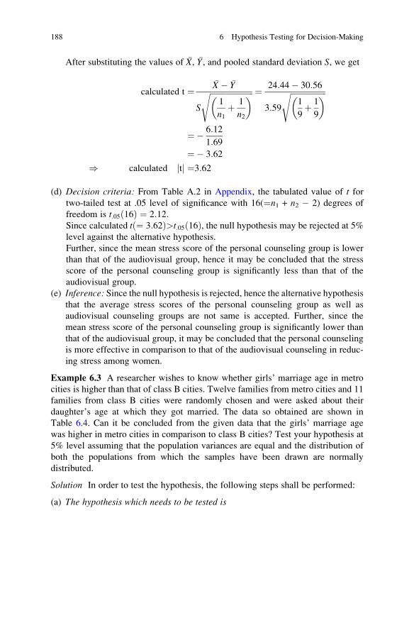
After substituting the values of �X, �Y, and pooled standard deviation S, we get
calculated t ¼�X � �Y
S
ffiffiffiffiffiffiffiffiffiffiffiffiffiffiffiffiffiffiffiffiffiffi1
n1þ 1
n2
� �s ¼ 24:44� 30:56
3:59
ffiffiffiffiffiffiffiffiffiffiffiffiffiffiffiffiffiffi1
9þ 1
9
� �s
¼� 6:12
1:69
¼� 3:62
) calculated tj j ¼3:62
(d) Decision criteria: From Table A.2 in Appendix, the tabulated value of t fortwo-tailed test at .05 level of significance with 16(¼n1 + n2 � 2) degrees of
freedom is t:05ð16Þ ¼ 2:12:Since calculated t ¼ 3:62ð Þ>t:05ð16Þ, the null hypothesis may be rejected at 5%
level against the alternative hypothesis.
Further, since the mean stress score of the personal counseling group is lower
than that of the audiovisual group, hence it may be concluded that the stress
score of the personal counseling group is significantly less than that of the
audiovisual group.
(e) Inference: Since the null hypothesis is rejected, hence the alternative hypothesisthat the average stress scores of the personal counseling group as well as
audiovisual counseling groups are not same is accepted. Further, since the
mean stress score of the personal counseling group is significantly lower than
that of the audiovisual group, it may be concluded that the personal counseling
is more effective in comparison to that of the audiovisual counseling in reduc-
ing stress among women.
Example 6.3 A researcher wishes to know whether girls’ marriage age in metro
cities is higher than that of class B cities. Twelve families from metro cities and 11
families from class B cities were randomly chosen and were asked about their
daughter’s age at which they got married. The data so obtained are shown in
Table 6.4. Can it be concluded from the given data that the girls’ marriage age
was higher in metro cities in comparison to class B cities? Test your hypothesis at
5% level assuming that the population variances are equal and the distribution of
both the populations from which the samples have been drawn are normally
distributed.
Solution In order to test the hypothesis, the following steps shall be performed:
(a) The hypothesis which needs to be tested is
188 6 Hypothesis Testing for Decision-Making

H0 : mMetro CitybmClass B City
against the alternative hypothesis
H0 : mMetro City>mClass B City
(b) The level of significance: 0.05(c) Statistical test: In this example, it is required to test one-tailed hypothesis for
comparing means of the two groups. Thus, as per the scheme of the test
selection shown in Fig. 6.1, a two-sample t-test for independent groups shallbe appropriate in this case which is
t ¼�X � �Y
S
ffiffiffiffiffiffiffiffiffiffiffiffiffiffiffiffiffiffiffiffiffiffi1
n1þ 1
n2
� �s
where the pooled standard deviation S is given by
S ¼ffiffiffiffiffiffiffiffiffiffiffiffiffiffiffiffiffiffiffiffiffiffiffiffiffiffiffiffiffiffiffiffiffiffiffiffiffiffiffiffiffiffiffiffiffiffiffin1 � 1ð ÞS21 þ n2 � 1ð ÞS22
n1 þ n2 � 2
s
To compute the value of t statistic, the mean and standard deviation of both the
groups along with the pooled standard deviation S need to be computed first
(Table 6.5).
Here n1 ¼ 12 and n2 ¼ 11 �X ¼ 34212
¼ 28:5 and �Y ¼ 27211
¼ 24:73
SX ¼ffiffiffiffiffiffiffiffiffiffiffiffiffiffiffiffiffiffiffiffiffiffiffiffiffiffiffiffiffiffiffiffiffiffiffiffiffiffiffiffiffiffiffiffiffiffiffiffiffiffiffiffiffiffi
1
n1 � 1
XX2 �
PXð Þ2
n1 n1 � 1ð Þ
s
¼ffiffiffiffiffiffiffiffiffiffiffiffiffiffiffiffiffiffiffiffiffiffiffiffiffiffiffiffiffiffiffiffiffiffiffiffiffiffiffiffiffiffi1
11� 9854� 342ð Þ2
12� 11
s¼
ffiffiffiffiffiffiffiffiffiffiffiffiffiffiffiffiffiffiffiffiffiffiffiffiffiffiffiffiffiffiffiffiffi895:82� 886:09
p
¼3:12
Table 6.4 Marital age of the girls
Metro city: 29, 28, 27, 31, 32, 25, 28, 24, 27, 30, 35, 26
Class B city: 28, 25, 24, 28, 22, 24, 23, 21, 25, 24, 28
Two-Sample t-Test for Unrelated Groups 189

Similarly
SY ¼ffiffiffiffiffiffiffiffiffiffiffiffiffiffiffiffiffiffiffiffiffiffiffiffiffiffiffiffiffiffiffiffiffiffiffiffiffiffiffiffiffiffiffiffiffiffiffiffiffiffiffiffiffiffi
1
n2 � 1
XY2 �
PYð Þ2
n2 n2 � 1ð Þ
s
¼ffiffiffiffiffiffiffiffiffiffiffiffiffiffiffiffiffiffiffiffiffiffiffiffiffiffiffiffiffiffiffiffiffiffiffiffiffiffiffiffiffiffi1
10� 6784� 272ð Þ2
11� 10
s¼
ffiffiffiffiffiffiffiffiffiffiffiffiffiffiffiffiffiffiffiffiffiffiffiffiffiffiffiffiffiffiffi678:4� 672:58
p
¼2:41
The pooled standard deviation S is equal to
S ¼ffiffiffiffiffiffiffiffiffiffiffiffiffiffiffiffiffiffiffiffiffiffiffiffiffiffiffiffiffiffiffiffiffiffiffiffiffiffiffiffiffiffiffiffiffiffiffiffin1 � 1ð ÞS2X þ n2 � 1ð ÞS2Y
n1 þ n2 � 2
s¼
ffiffiffiffiffiffiffiffiffiffiffiffiffiffiffiffiffiffiffiffiffiffiffiffiffiffiffiffiffiffiffiffiffiffiffiffiffiffiffiffiffiffiffiffiffiffiffiffi11� 3:122 þ 10� 2:412
12þ 11� 2
s
¼ffiffiffiffiffiffiffiffiffiffiffiffiffiffiffiffiffiffiffiffiffiffiffiffiffiffiffiffiffiffiffi107:08þ 58:08
21
r¼ 2:80
Since t-test can only be applied if the variance of both the populations is same,
this hypothesis can be tested by using the F-test.
Thus, F ¼ S2XS2Y
¼ 3:122
2:412¼ 1:67
The tabulated value of F can be seen from Table A.4 in Appendix.
Thus, tabulated F.05(11,10) ¼ 2.85
Since calculated value of F is less than that of tabulated F, hence hypothesis ofequality of variances in two groups may not be rejected, and therefore, the two-
sample t-test for independent samples can be applied in this example.
After substituting the values of �X, �Y, and pooled standard deviation, S we get
Table 6.5 Computation for
mean and standard deviationMetro city Class B city
X X2 Y Y2
29 841 28 784
28 784 25 625
27 729 24 576
31 961 28 784
32 1,024 22 484
25 625 24 576
28 784 23 529
24 576 21 441
27 729 25 625
30 900 24 576
35 1,225 28 784
26 676PX ¼342
PX2 ¼ 9; 854
PY ¼272
PY2 ¼ 6; 784
190 6 Hypothesis Testing for Decision-Making

calculated t ¼�X � �Y
S
ffiffiffiffiffiffiffiffiffiffiffiffiffiffiffiffiffiffiffiffiffiffi1
n1þ 1
n2
� �s ¼ 28:5� 24:73
2:80
ffiffiffiffiffiffiffiffiffiffiffiffiffiffiffiffiffiffiffiffiffiffiffi1
12þ 1
11
� �s
¼ 3:77
2:80� 0:42
¼3:21
(d) Decision criteria: From Table A.2 in Appendix, the tabulated value of t for one-tailed test at .05 level of significance with 21(¼n1 + n2 � 2) degrees of free-
dom is t:05ð21Þ ¼ 1:721. Similarly for one-tailed test, tabulated value of t at .01level of significance is t:01ð21Þ ¼ 2:518:Since calculated t ¼ 3:21ð Þ>t:05ð21Þ, the null hypothesis may be rejected at 5%
level. Further, calculated value of t is also less than that of tabulated value of t at1% level as well; hence, t-value is also significant at 1% level.
(e) Inference: Since the null hypothesis is rejected, hence the alternative hypothesisthat the marriage age of the girls in metro cities is higher than that of class B
cities is accepted. It may thus be concluded that girls in metro cities prefers to
marry late in age in comparison to that of class B cities.
Paired t-Test for Related Groups
Paired t-test is used to test the null hypothesis that the difference between the two
responses measured on the same experimental units has a mean value of zero. This
statistical test is normally used to test the research hypothesis as to whether the
posttreatment response is better than the pretreatment response. Paired t-test is usedin all those situations where there is only one experimental group and no control
group. The question which is tested here is to know whether the treatment is
effective or not. This is done by measuring the responses of the subjects in the
experimental group before and after the treatment. There can be several instances in
which the paired t-test may be used. Such situations may be, for instance, to see the
effectiveness of management development program on the functional efficiency,
effectiveness of the weight training program in weight reduction, effectiveness of
the psychological training in enhancing memory retention power, etc.
The paired t-test is also known as “repeated measures” t-test. In using the pairedt-test, the data must be obtained in pair on the same set of subjects before and after
the experiment.
While applying the paired t-test for two related groups, the pairwise differences,
di, is computed for all n paired data. The mean, �d and standard deviation, Sd, of thedifferences di are calculated. Thus, paired t-statistic is computed as follows:
t ¼�d
Sd=ffiffiffin
p (6.3)
where “t” follows the Student’s t-distribution with n � 1 degrees of freedom.
Two-Sample t-Test for Unrelated Groups 191

An assumption in using the paired t-test is that the difference di follows the
normal distribution. An experiment where paired difference is computed is often
more powerful, since it can eliminate differences in the samples that increase the
total variances2. When the comparison is made between groups (of similar experi-
mental units), it is called blocking. The paired difference experiment is an example
of a randomized block experiment.
Note: The blocking has to be done before the experiment is performed.
Assumptions in Using Paired t-Test
While using the paired t-test, the following assumptions need to be satisfied:
1. The distribution of the population is normal.
2. The distribution of scores obtained by pairwise difference is normal, and the
differences are a random sample.
3. Cases must be independent of each other.
Remark: If the normality assumption is not fulfilled, you may use the nonparamet-
ric Wilcoxon sign rank test for paired difference designs.
Testing Protocol in Using Paired t-Test
Testing protocol of using paired t-test is similar to that of two-sample t-test forindependent groups discussed above. In applying paired t-test, the only difference isthat the test statistic is
t ¼�d
Sd=ffiffiffin
p
instead of the one used in two-sample t-test. Further, in paired t-test, the degrees offreedom are n � 1. While using paired t-test, one should normally construct the
two-tailed test first, and if the difference is significant, then by looking to the values
of the samples mean of the pre- and posttesting responses, one may interpret as to
which group mean is higher than the other. In general using one-tailed test should
be avoided until there is strong evidence that the difference can go only in one
direction. In one-tailed test, the probability of rejecting the correct null hypothesis
becomes more in comparison to two-tailed test for the same level of significance.
192 6 Hypothesis Testing for Decision-Making
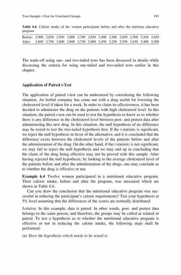
The trade-off using one- and two-tailed tests has been discussed in details while
discussing the criteria for using one-tailed and two-tailed tests earlier in this
chapter.
Application of Paired t-Test
The application of paired t-test can be understood by considering the following
situation. An herbal company has come out with a drug useful for lowering the
cholesterol level if taken for a week. In order to claim its effectiveness, it has been
decided to administer the drug on the patients with high cholesterol level. In this
situation, the paired t-test can be used to test the hypothesis to know as to whether
there is any difference in the cholesterol level between post- and pretest data after
administering this new drug. In this situation, the null hypothesis of no difference
may be tested to test the two-tailed hypothesis first. If the t-statistic is significant,
we reject the null hypothesis in favor of the alternative, and it is concluded that the
difference exists between the cholesterol levels of the patients before and after
the administration of the drug. On the other hand, if the t-statistic is not significant,we may fail to reject the null hypothesis and we may end up in concluding that
the claim of the drug being effective may not be proved with this sample. After
having rejected the null hypothesis, by looking to the average cholesterol level of
the patients before and after the administration of the drugs, one may conclude as
to whether the drug is effective or not.
Example 6.4 Twelve women participated in a nutritional educative program.
Their calorie intake, before and after the program, was measured which are
shown in Table 6.6.
Can you draw the conclusion that the nutritional educative program was suc-
cessful in reducing the participant’s calorie requirements? Test your hypothesis at
5% level assuming that the differences of the scores are normally distributed.
Solution In this example, data is paired. In other words, post- and pretest data
belongs to the same person, and therefore, the groups may be called as related or
paired. To test a hypothesis as to whether the nutritional educative program is
effective or not in reducing the calorie intake, the following steps shall be
performed:
(a) Here the hypothesis which needs to be tested is
Table 6.6 Calorie intake of the women participants before and after the nutrition educative
program
Before: 2,900 2,850 2,950 2,800 2,700 2,850 2,400 2,200 2,650 2,500 2,450 2,650
After: 2,800 2,750 2,800 2,800 2,750 2,800 2,450 2,250 2,550 2,450 2,400 2,500
Two-Sample t-Test for Unrelated Groups 193

H0 : mD ¼ 0 Difference of means of the two groups is zero:ð Þagainst the alternative hypothesis
H1 : mD 6¼ 0 Difference of means of the two groups is not equal to zero:ð Þ
(b) The level of significance: 0.05(c) Statistical test: In this example, it is required to test the effectiveness of the
nutritional educative program in reducing the calorie consumption in diet. Here
the null hypothesis that there is no difference in the means of the two groups is
to be tested against the alternative hypothesis that there is a difference. Once the
null hypothesis is rejected, then on the basis of mean values of the pre- and
posttesting data of calorie consumption, the conclusion would be drawn as to
whether the program was effective or not.
Thus, first a two-tailed test will be used, and if the null hypothesis is rejected
against the alternative hypothesis, then the directional interpretation would be
made by looking to the mean values. It is because of the fact that if the t-statisticis significant in two-tailed test, then it will also be significant at one-tailed test.
This can be understood like this: for the two-tailed test, the critical value ta=2 at alevel of significance will always be greater than that of the critical value ta in
one-tailed test. And therefore, if the calculated value of t is greater than ta=2, it
will also be greater than ta.Since this example is a case of paired samples, hence as per the scheme of the
test selection shown in Fig. 6.1, the paired t-test for related groups shall be
appropriate in this case which is given by
t ¼�d
Sd=ffiffiffin
p
where �d is the mean of the difference between X and Y, and Sd is the standard
deviation of these differences as given by
Sd ¼ffiffiffiffiffiffiffiffiffiffiffiffiffiffiffiffiffiffiffiffiffiffiffiffiffiffiffiffiffiffiffiffiffiffiffiffiffiffiffiffiffiffiffiffiffiffiffi1
n� 1
Xd2 � ðP dÞ2
nðn� 1Þ
s
The �d and Sd shall be computed first to find the value of t-statistic (Table 6.7).
Remark: Difference d can be computed by subtracting postdata from
predata or vice versa because two-tailed test is being used here
Here number of paired data, n ¼ 12,
�d ¼ 600
12¼ 50
and
194 6 Hypothesis Testing for Decision-Making
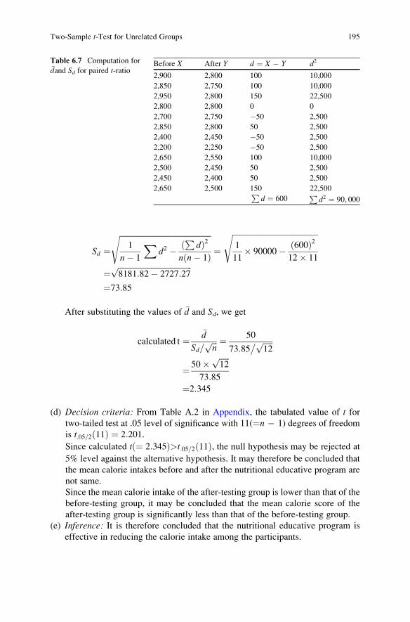
Sd ¼ffiffiffiffiffiffiffiffiffiffiffiffiffiffiffiffiffiffiffiffiffiffiffiffiffiffiffiffiffiffiffiffiffiffiffiffiffiffiffiffiffiffiffiffiffiffiffi1
n� 1
Xd2 �
Pdð Þ2
n n� 1ð Þ
s¼
ffiffiffiffiffiffiffiffiffiffiffiffiffiffiffiffiffiffiffiffiffiffiffiffiffiffiffiffiffiffiffiffiffiffiffiffiffiffiffiffiffiffiffiffi1
11� 90000� 600ð Þ2
12� 11
s
¼ffiffiffiffiffiffiffiffiffiffiffiffiffiffiffiffiffiffiffiffiffiffiffiffiffiffiffiffiffiffiffiffiffiffiffiffiffiffi8181:82� 2727:27
p
¼73:85
After substituting the values of �d and Sd, we get
calculated t ¼�d
Sdffiffiffin
p=
¼ 50
73:85ffiffiffiffiffi12
p�¼ 50� ffiffiffiffiffi
12p
73:85
¼2:345
(d) Decision criteria: From Table A.2 in Appendix, the tabulated value of t fortwo-tailed test at .05 level of significance with 11(¼n � 1) degrees of freedom
is t:05=2ð11Þ ¼ 2:201.
Since calculated t ¼ 2:345ð Þ>t:05=2ð11Þ, the null hypothesis may be rejected at
5% level against the alternative hypothesis. It may therefore be concluded that
the mean calorie intakes before and after the nutritional educative program are
not same.
Since the mean calorie intake of the after-testing group is lower than that of the
before-testing group, it may be concluded that the mean calorie score of the
after-testing group is significantly less than that of the before-testing group.
(e) Inference: It is therefore concluded that the nutritional educative program is
effective in reducing the calorie intake among the participants.
Table 6.7 Computation for�dand Sd for paired t-ratio
Before X After Y d ¼ X � Y d2
2,900 2,800 100 10,000
2,850 2,750 100 10,000
2,950 2,800 150 22,500
2,800 2,800 0 0
2,700 2,750 �50 2,500
2,850 2,800 50 2,500
2,400 2,450 �50 2,500
2,200 2,250 �50 2,500
2,650 2,550 100 10,000
2,500 2,450 50 2,500
2,450 2,400 50 2,500
2,650 2,500 150 22,500Pd ¼ 600
Pd2 ¼ 90; 000
Two-Sample t-Test for Unrelated Groups 195

Solved Example of Testing Single Group Mean with SPSS
Example 6.5 The age of the 15 randomly chosen employees of an organization is
shown in Table 6.8. Can it be concluded that the average age of the employees in
the organization is 28 years? Test your hypothesis at 5% level and interpret your
findings.
Solution The hypothesis that needs to be tested here is
H0 : m ¼ 28
against the alternative hypothesis
H1 : m 6¼ 28
After using the SPSS commands as mentioned below for testing the population
mean to be equal to 28, the output will generate the value of t-statistic along with itsp value. If p value is less than .05, then the t-statistic will be significant and the nullhypothesis shall be rejected at 5% level in favor of alternative hypothesis; other-
wise, we would fail to reject the null hypothesis.
Computation of t-Statistic and Related Outputs
(a) Preparing Data FileBefore using the SPSS commands for computing the value of t-statistic and
other related statistics for single group, a data file needs to be prepared. The
following steps will help you to prepare the data file:
Table 6.8 Data on age 27
31
34
29
28
34
33
36
26
28
29
36
35
31
36
196 6 Hypothesis Testing for Decision-Making

(i) Starting the SPSS: Use the following command sequence to start SPSS:
Start ! All Programs ! IBM SPSS Statistics ! IBM SPSS
Statistics 20
After checking the option Type in Data on the screen you will be taken to
the Variable View option for defining the variables in the study.
(ii) Defining variables: There is only one variable in this example which needs
to be defined in SPSS along with its properties. Since the variable is
measured on interval scale, hence will be defined as ‘Scale’ variable. The
procedure of defining the variable in the SPSS is as follows:
1. Click Variable View to define the variable and its properties.
2. Write short name of the variable as Age under the column headingName.
3. Under the column heading Label, define full name of the variable as
Employees’ Age.4. Under the column heading Measure, select the option ‘Scale’ for the
variable.
5. Use default entries in all other columns.
After defining the variable in variable view, the screen shall look like Fig. 6.5.
(iii) Entering data: After defining the variable in the Variable View, click DataView on the left bottom of the screen to enter the data. Enter the data for the
variable column wise. After entering the data, the screen will look like
Fig. 6.6. Save the data file in the desired location before further processing.
(b) SPSS Commands for Computing t-StatisticAfter entering the data in the data view, follow these steps for computing t-statistic:
(i) Initiating the SPSS commands for one-sample t-test: In data view, go to the
following commands in sequence:
Analyze ⇨ Compare Means ⇨ One-Sample t Test
The screen shall look like Fig. 6.7 as shown below.
(ii) Selecting variables for t-statistic: After clicking the One-Sample t Testoption you will be taken to the next screen for selecting variable for
computing t-statistic. Select the variable Age from left panel and bring it
to the right panel by clicking the arrow sign. In case of computing t-valuefor more than one variable simultaneously, all the variables can be selected
together. The screen shall look like Fig. 6.8.
(iii) Selecting the options for computation: After selecting the variable, option
needs to be defined for the one-sample t-test. Do the following:
– In the screen shown in Fig. 6.8, enter the ‘test value’ as 28. This is the
assumed population mean age that we need to verify in the hypothesis.
– Click the tag Options, you will get the screen shown in Fig. 6.9. Enter
the confidence interval as 95% and click Continue and then you will betaken back to the screen shown in Fig. 6.8.
Solved Example of Testing Single Group Mean with SPSS 197

The confidence interval is chosen to get the confidence limits of mean
based on sample data. Since in this example the null hypothesis needs to
be tested at 5% level, choose the confidence interval as 95%.
– Click OK.
(c) Getting the OutputAfter clicking the OK tag in Fig. 6.8, you will get the output window. In the
output window, the relevant outputs can be selected by using the right click of
Fig. 6.5 Defining variable and its characteristics for the data shown in Table 6.8
Fig. 6.6 Screen showing
entered data for the age
variable in the data view
198 6 Hypothesis Testing for Decision-Making

Fig. 6.7 Screen showing SPSS commands for one sample t-test
Fig. 6.8 Screen showing selection of variable for one-sample t-test
Solved Example of Testing Single Group Mean with SPSS 199

the mouse, and the content may be copied in the word file. The output panel
shall have the following results:
1. Sample statistics showing mean, standard deviation, and standard error
2. Table showing the value of t and its significance level
Fig. 6.9 Screen showing options for computing one-sample t-test and selecting significance level
Table 6.9 One-sample statistics
N Mean Std. deviation Std. error mean
Employees’ age 15 31.5333 3.54293 .91478
Table 6.10 One-sample t test
Test value ¼ 28
95% confidence interval
of the difference
t df Sig. (two-tailed) Mean difference Lower Upper
Employees’ age 3.862 14 .002 3.53333 1.5713 5.4953
Table 6.11 t-table for thedata on employees’ age
Mean SD Mean diff. t-value p value
31.53 3.54 3.53 3.862 .002
200 6 Hypothesis Testing for Decision-Making
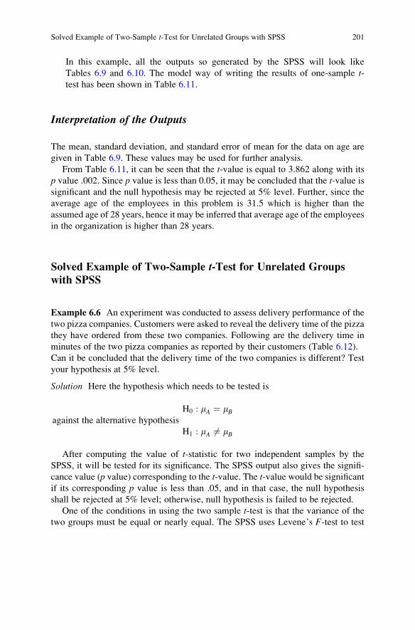
In this example, all the outputs so generated by the SPSS will look like
Tables 6.9 and 6.10. The model way of writing the results of one-sample t-test has been shown in Table 6.11.
Interpretation of the Outputs
The mean, standard deviation, and standard error of mean for the data on age are
given in Table 6.9. These values may be used for further analysis.
From Table 6.11, it can be seen that the t-value is equal to 3.862 along with its
p value .002. Since p value is less than 0.05, it may be concluded that the t-value issignificant and the null hypothesis may be rejected at 5% level. Further, since the
average age of the employees in this problem is 31.5 which is higher than the
assumed age of 28 years, hence it may be inferred that average age of the employees
in the organization is higher than 28 years.
Solved Example of Two-Sample t-Test for Unrelated Groups
with SPSS
Example 6.6 An experiment was conducted to assess delivery performance of the
two pizza companies. Customers were asked to reveal the delivery time of the pizza
they have ordered from these two companies. Following are the delivery time in
minutes of the two pizza companies as reported by their customers (Table 6.12).
Can it be concluded that the delivery time of the two companies is different? Test
your hypothesis at 5% level.
Solution Here the hypothesis which needs to be tested is
H0 : mA ¼ mBagainst the alternative hypothesis
H1 : mA 6¼ mB
After computing the value of t-statistic for two independent samples by the
SPSS, it will be tested for its significance. The SPSS output also gives the signifi-
cance value (p value) corresponding to the t-value. The t-value would be significantif its corresponding p value is less than .05, and in that case, the null hypothesis
shall be rejected at 5% level; otherwise, null hypothesis is failed to be rejected.
One of the conditions in using the two sample t-test is that the variance of the
two groups must be equal or nearly equal. The SPSS uses Levene’s F-test to test
Solved Example of Two-Sample t-Test for Unrelated Groups with SPSS 201
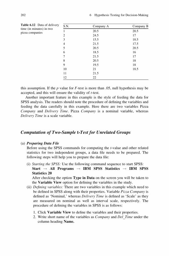
this assumption. If the p value for F-test is more than .05, null hypothesis may be
accepted, and this will ensure the validity of t-test.Another important feature in this example is the style of feeding the data for
SPSS analysis. The readers should note the procedure of defining the variables and
feeding the data carefully in this example. Here there are two variables Pizza
Company and Delivery Time. Pizza Company is a nominal variable, whereas
Delivery Time is a scale variable.
Computation of Two-Sample t-Test for Unrelated Groups
(a) Preparing Data FileBefore using the SPSS commands for computing the t-value and other related
statistics for two independent groups, a data file needs to be prepared. The
following steps will help you to prepare the data file:
(i) Starting the SPSS: Use the following command sequence to start SPSS:
Start ! All Programs ! IBM SPSS Statistics ! IBM SPSS
Statistics 20
After checking the option Type in Data on the screen you will be taken to
the Variable View option for defining the variables in the study.
(ii) Defining variables: There are two variables in this example which need to
be defined in SPSS along with their properties. Variable Pizza Company isdefined as ‘Nominal,’ whereas Delivery Time is defined as ‘Scale’ as they
are measured on nominal as well as interval scale, respectively. The
procedure of defining the variables in SPSS is as follows:
1. Click Variable View to define the variables and their properties.
2. Write short name of the variables as Company and Del_Time under thecolumn heading Name.
Table 6.12 Data of delivery
time (in minutes) in two
pizza companies
S.N. Company A Company B
1 20.5 20.5
2 24.5 17
3 15.5 18.5
4 21.5 17.5
5 20.5 20.5
6 18.5 16
7 21.5 17
8 20.5 18
9 19.5 18
10 21 18.5
11 21.5
12 22
202 6 Hypothesis Testing for Decision-Making

3. Under the column heading Label, full names of these variables may be
defined as Pizza Company and Delivery Time, respectively. Readersmay choose some other names of these variables as well.
4. For the variable Company, double-click the cell under the column
heading Values and add the following values to different levels:
Value Label
1 Company A
2 Company B
The screen for defining the values can be seen in Fig. 6.10.
5. Under the column headingMeasure, select the option ‘Nominal’ for the
Company variable and ‘Scale’ for the Del_Time variable.6. Use default entries in rest of the columns.
After defining the variables in variable view, the screen shall look like
Fig. 6.10
(iii) Entering dataAfter defining both the variables in Variable View, click Data View on
the left corner in the bottom of the screen shown in Fig. 6.10 to open the
data entry format column wise. For the Company variable, type first twelvescores as 1 and the next ten scores as 2 in the column. This is because the
value ‘1’ denotes Company A and there are 12 delivery time scores
reported by the customers. Similarly, the value ‘2’ denotes Company B
and there are 10 delivery time scores as reported by the customers. After
entering the data, the screen will look like Fig. 6.11.
Fig. 6.10 Defining variables along with their characteristics
Solved Example of Two-Sample t-Test for Unrelated Groups with SPSS 203

(b) SPSS Commands for Two-Sample t-TestAfter preparing the data file in data view, take the following steps for two-
sample t-test:
(i) Initiating the SPSS commands for two-sample t-test: In data view, click the
following commands in sequence:
Analyze ⇨ Compare means ⇨ Independent-Samples t testThe screen shall look like Fig. 6.12.
(ii) Selecting variables for analysis: After clicking the Independent-Samples
t test option, you will be taken to the next screen for selecting variables forthe two-sample t-test. Select the variable Delivery Time from left panel and
Fig. 6.11 Screen showing
entered data for company and
delivery time in the data view
204 6 Hypothesis Testing for Decision-Making
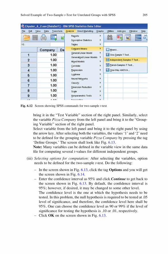
bring it in the “Test Variable” section of the right panel. Similarly, select
the variable Pizza Company from the left panel and bring it to the “Group-
ing Variable” section of the right panel.
Select variable from the left panel and bring it to the right panel by using
the arrow key. After selecting both the variables, the values ‘1’ and ‘2’ need
to be defined for the grouping variable Pizza Company by pressing the tag
‘Define Groups.’ The screen shall look like Fig. 6.13.
Note: Many variables can be defined in the variable view in the same data
file for computing several t-values for different independent groups.
(iii) Selecting options for computation: After selecting the variables, option
needs to be defined for the two-sample t-test. Do the following:
– In the screen shown in Fig. 6.13, click the tag Options and you will get
the screen shown in Fig. 6.14.
– Enter the confidence interval as 95% and click Continue to get back to
the screen shown in Fig. 6.13. By default, the confidence interval is
95%; however, if desired, it may be changed to some other level.
The confidence level is the one at which the hypothesis needs to be
tested. In this problem, the null hypothesis is required to be tested at .05
level of significance, and therefore, the confidence level here shall be
95%. One can choose the confidence level as 90 or 99% if the level of
significance for testing the hypothesis is .10 or .01, respectively.
– Click OK on the screen shown in Fig. 6.13.
Fig. 6.12 Screen showing SPSS commands for two-sample t-test
Solved Example of Two-Sample t-Test for Unrelated Groups with SPSS 205

(c) Getting the OutputClicking the OK key in Fig. 6.14 will lead you to the output window. In the
output window of the SPSS, the relevant outputs may be selected by using the
Fig. 6.13 Screen showing selection of variable for two-sample t-test for unrelated groups
Fig. 6.14 Screen showing the option for choosing the significance level
206 6 Hypothesis Testing for Decision-Making

right click of the mouse, and it may be copied in the word file. The output panel
shall have the following results:
1. Descriptive statistics for the data in different groups
2. ‘F-’ and ‘t-’values for testing the equality of variances and equality of
means, respectively
(i) In this example, all the outputs so generated by the SPSS will look like
Tables 6.13 and 6.14. The model way of writing the results of two-sample t-test for unrelated samples has been shown in Table 6.15.
Interpretation of the Outputs
The following interpretations can be made on the basis of the results shown in the
above outputs:
1. Table 6.13 shows the mean, standard deviation, and standard error of the mean
for the data on delivery time of both the pizza companies. The mean delivery
time of the company B is less than that of the delivery time of company A.
However, whether this difference is significant or not shall be revealed by
looking to the t-value and its associated p value. However, if the t-value is not
significant, no one should draw the conclusion about the delivery time of the
pizza companies by looking to the sample means.
Table 6.13 Descriptive statistics of the groups
Pizza company N Mean Std. deviation Std. error mean
Delivery time in sec A 12 20.58 2.16 .62412
B 10 18.15 1.45 .45977
Table 6.14 F- and t-table for testing the equality of variances and equality of means of two
unrelated groups
Levene’s
test for
equality of
variance t-test for equality of means
95%
confidence
interval of the
difference
F Sig. t df
Sig. (two-
tailed)
Mean
diff.
SE
diff. Lower Upper
Delivery time in sec.
Equal variances
assumed
.356 .557 3.028 20 .007 2.43 .804 0.76 4.11
Equal variances not
assumed
3.139 19.3 .005 2.43 .775 0.81 4.05
Solved Example of Two-Sample t-Test for Unrelated Groups with SPSS 207

2. One of the conditions for using the two-sample t-ratio for unrelated groups is thatthe variance of the two groups must be equal. To test the equality of variances,
Levene’s test was used. In Table 6.14, F-value is .356 which is insignificant as
the p value is .557 which is more than .05. Thus, the null hypothesis of equality
of variances may be accepted, and it is concluded that the variances of the two
groups are equal.
3. It can be seen from Table 6.15 that the value of t-statistic is 3.028. This t-value issignificant as its p value is 0.007 which is less than .05. Thus, the null hypothesisof equality of population means of two groups is rejected, and it may be
concluded that the average delivery time of the pizza in both the companies is
different. Further, average delivery time of the company B is less than that of the
company A, and therefore, it may be concluded that the delivery of pizza by the
company B to their customers is faster than that of the company A.
Remark: The readers can note that initially the two-tailed hypothesis was tested in
this example, but the final conclusion has beenmade similar to the one-tailed test. This
is because of the fact that if the t-statistic is significant in two-tailed test then it will alsobe significant at one-tailed test. To make it clearer, let us consider that for two-tailed
test, the critical value is ta=2 at level of significance. This value will always be greater
than that of the critical value of ta in one-tailed test, and therefore, if the calculated
value of t is greater than ta=2, it will also be greater than ta.
Solved Example of Paired t-Test with SPSS
Example 6.7 An experiment was conducted to know the impact of new advertise-
ment campaign on sale of television of a particular brand. The number of television
units sold on 12 consecutive working days before and after launching the advertise-
ment campaign in a city was recorded. The data obtained are shown in Table 6.16.
Solution Here the hypothesis which needs to be tested is
H0 : mD ¼ 0 Difference of average sales after and before the advertisement is zero:ð Þ
against the alternative hypothesis
Table 6.15 t-table for the data on delivery time along with F-value
Groups Means S.D. Mean. diff SE of mean diff t-value p value F-value p value
Company A 20.58 2.16 2.43 .804 3.028 .007 .356 .557
Company B 18.15 1.45
208 6 Hypothesis Testing for Decision-Making

H1 : mD 6¼ 0 Difference of average sales after and before the advertisement isðnot equal to zero:Þ
After getting the value of t-statistic for paired sample in the output of SPSS, it
needs to be tested for its significance. The output so generated by the SPSS also
gives the significance level (p value) along with t-value. The null hypothesis may be
rejected if the p value is less than .05; otherwise, it is accepted. If the null hypothesisis rejected, an appropriate conclusion may be drawn regarding the effectiveness of
the advertisement campaign by looking to the mean values of the sales before and
after the advertisement.
In this problem, there are two variables TV Sold before Advertisement and TV Soldafter Advertisement. For both these variables, data shall be entered in two different
columns unlike the way it was entered in two-sample t-test for unrelated groups.
Computation of Paired t-Test for Related Groups
(a) Preparing Data FileThe data file needs to be prepared first for using the SPSS commands for the
computation of t-value and other related statistics. Follow the below-mentioned
steps in preparing the data file.
(i) Starting the SPSS: Follow the below-mentioned command sequence to start
SPSS on your computer:
Start ! All Programs ! IBM SPSS Statistics ! IBM SPSS
Statistics 20
(ii) Defining variables: In this example, two variables TV Sold before Adver-tisement and TV Sold after Advertisement need to be defined along with
their properties. Both these variables are scalar as they are measured on
Table 6.16 Number of TV
units sold in a city before and
after the advertisement
campaign
Days Before advertisement After advertisement
1 25 28
2 36 42
3 22 38
4 26 40
5 18 35
6 8 12
7 23 29
8 31 52
9 25 26
10 22 26
11 20 25
12 5 7
Solved Example of Paired t-Test with SPSS 209

ratio scale. These variables can be defined along with their properties in
SPSS by using the following steps:
1. After clicking the Type in Data above, click theVariable View to define
the variables and their properties.
2. Write short name of the variables as After_Ad and Before_Ad under the
column heading Name.
3. Under the column heading Label, full name of these variables may be
defined as TV Sold before Advertisement and TV Sold after Advertise-ment, respectively. Readers may choose some other names of these
variables if so desired.
4. Under the column heading Measure, select the option ‘Scale’ for both
the variables.
5. Use default entries in rest of the columns.
After defining the variables in variable view, the screen shall look like
Fig. 6.15.
(iii) Entering the dataOnce both these variables are defined in the Variable View, click Data
View on the left corner in the bottom of the screen as shown in Fig. 6.15 to
open the format for entering the data column wise. For both these
variables, data is entered column wise. After entering the data, the screen
will look like Fig. 6.16.
(b) SPSS Commands for Paired t-TestAfter entering all the data in the data view, take following steps for paired t-test.
(i) Initiating SPSS commands for paired t-test: In data view, click the follow-
ing commands in sequence:
Analyze ! Compare means ! Paired-Samples t Test
The screen shall look like Fig. 6.17.
Fig. 6.15 Variables along with their characteristics for the data shown in Table 6.16
210 6 Hypothesis Testing for Decision-Making

Fig. 6.16 Screen showing
entered data on TV sales
before and after the
advertisement campaign
Fig. 6.17 Screen showing SPSS commands for paired t-test
Solved Example of Paired t-Test with SPSS 211
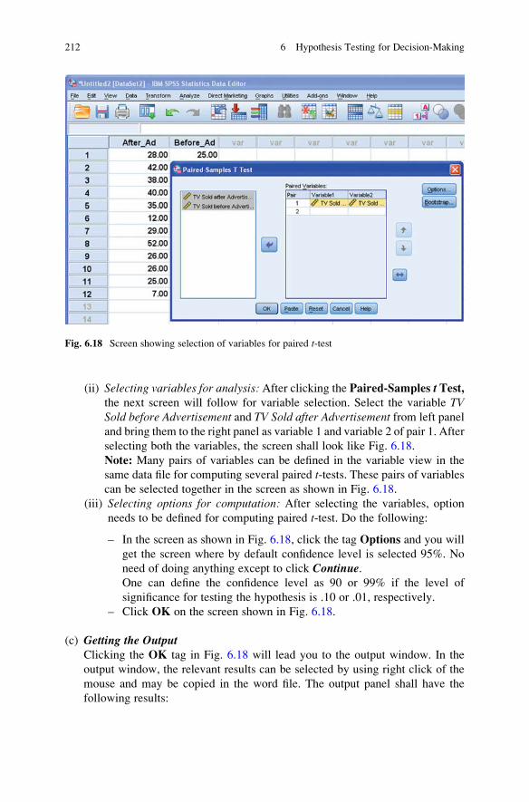
(ii) Selecting variables for analysis: After clicking the Paired-Samples t Test,the next screen will follow for variable selection. Select the variable TVSold before Advertisement and TV Sold after Advertisement from left panel
and bring them to the right panel as variable 1 and variable 2 of pair 1. After
selecting both the variables, the screen shall look like Fig. 6.18.
Note: Many pairs of variables can be defined in the variable view in the
same data file for computing several paired t-tests. These pairs of variablescan be selected together in the screen as shown in Fig. 6.18.
(iii) Selecting options for computation: After selecting the variables, option
needs to be defined for computing paired t-test. Do the following:
– In the screen as shown in Fig. 6.18, click the tag Options and you will
get the screen where by default confidence level is selected 95%. No
need of doing anything except to click Continue.One can define the confidence level as 90 or 99% if the level of
significance for testing the hypothesis is .10 or .01, respectively.
– Click OK on the screen shown in Fig. 6.18.
(c) Getting the OutputClicking the OK tag in Fig. 6.18 will lead you to the output window. In the
output window, the relevant results can be selected by using right click of the
mouse and may be copied in the word file. The output panel shall have the
following results:
Fig. 6.18 Screen showing selection of variables for paired t-test
212 6 Hypothesis Testing for Decision-Making

1. Paired samples statistics
2. Paired t-test table
In this example, all the outputs so generated by the SPSS will look like
Tables 6.17 and 6.18.
Interpretation of the Outputs
The following interpretations can be made on the basis of the results shown in the
above output:
1. The values of the mean, standard deviation, and standard error of the mean for
the data on TV sales before and after the advertisement are shown in Table 6.17.
These values can be used to draw conclusion as to whether the advertisement
campaign was effective or not.
2. It can be seen from Table 6.18 that the value of t-statistic is 4.204. This t-value issignificant as the p value is 0.001 which is less than .05. Thus, the null hypothesisof equality of average TV sales before and after advertisement is rejected, and
therefore, it may be concluded that the average sale of the TV units before and
after the advertisement is not same.
Further, by looking to the values of the mean sales of the TV units before and
after advertisement in Table 6.17, you may note that the average sales have
increased after the advertisement campaign. Since the null hypothesis has been
rejected, it may thus be concluded that the increase in the TV units has been
significantly increased due to advertisement campaign.
Table 6.17 Paired sample statistics
Mean N SD SE(mean)
Pair 1
TV sold before advertisement 21.75 12 8.61 2.49
TV sold after advertisement 30.00 12 12.55 3.62
Table 6.18 Paired t-test for the data on number of TV sold
Paired differences
95% confidence
interval of the
difference
Mean SD SE(M) Lower Upper t df Sig.(two-tailed)
Pair 1
Before advertisement 8.25 6.797 1.96 3.93 12.57 4.204 11 .001
After advertisement
Solved Example of Paired t-Test with SPSS 213

You may notice that we started with testing two-tailed test but ended up in
testing one-tailed test. This is because of the fact that if the t-value is significantat 5% level in two-tailed test, then this will also be significant in one-tailed test.
Summary of SPSS Commands for t-Tests
(a) For One-Sample t-Test
(i) Start the SPSS by using the following commands:
Start ! All Programs ! IBM SPSS Statistics ! IBM SPSS
Statistics 20
(ii) Click Variable View tag and define the variable Age.(iii) Once the variables are defined, type the data for each variable by clicking
Data View.
(iv) In the data view, follow the below-mentioned command sequence for
computing one-sample t-test:
Analyze Compare Means One-Sample t Test
(v) Select the variable Age from left panel to the right panel by using the arrow
command.
(vi) Enter the test value as 28. This is the population mean age which is
required to be tested.
(vii) By clicking the tag Options, ensure that confidence interval is selected as
95% and click Continue. Confidence level can be entered as 90 or 99% if
the level of significance for testing the hypothesis is .10 or .01,
respectively.
(viii) Press OK for output.
(b) For Two-Sample t-Test for Unrelated Groups
(i) Start the SPSS the way it is done in case of one-sample t-test.(ii) In the variable view, define Company and Del_Time as a ‘Nominal’ and
‘Scale’ variables, respectively.
(iii) In the variable view under column heading Values, define the values ‘1’
for Company A and ‘2’ for Company B for the variable Company.(iv) In the data view, feed the data of Company A as 1 for first twelve entries (as
there are twelve scores in the Company A) and 2 as next ten entries (as ten
scores are in Company B) column wise under the column Company. Underthe columnDel_Time, enter the first group of delivery time data and then in
the same column, enter the second group of delivery time data.
(v) In the data view, follow the below-mentioned command sequence for
computing the value of t:
Analyze ! Compare means ! Independent-Samples t test
214 6 Hypothesis Testing for Decision-Making

(vi) Select the Company and Del_Time variables from left panel and bring
them in the “Test Variable” and “Grouping Variable” sections of the right
panel, respectively.
(vii) Define the values 1 and 2 as two groups for the grouping variable
Company.(viii) By clicking the tagOptions, ensure that confidence interval is selected as
95% and click Continue.(ix) Press OK for output.
(c) For Paired t-Test
(i) Start the SPSS the way it is done in case of one-sample t-test.(ii) In variable view, define the variables After_Ad and Before_Ad as scale
variables.
(iii) In the data view, follow the below-mentioned command sequence for
computing the value of t after entering the data for both the variables:
Analyze ! Compare means ! Paired-Samples t Test(iv) Select the variables After_Ad and Before_Ad from left panel and bring
them to the right panel as variable 1 and variable 2 of pair 1.
(v) By clicking the tag Options, ensure that confidence interval is selected as
95% and click Continue.(vi) Press OK for output.
Exercise
Short-Answer Questions
Note: Write the answer to each of the following questions in not more than 200
words.
Q.1. What do you mean by pooled standard deviation? How will you compute it?
Q.2. Discuss the criteria of choosing a statistical test in testing hypothesis
concerning mean and variances.
Q.3. What are the various considerations in constructing null and alternative
hypotheses?
Q.4. What are the various steps in testing a hypothesis?
Q.5. Discuss the advantages and disadvantages of one- and two-tailed tests.
Q.6. Explain the situations in which one- and two-tailed tests should be used.
Q.7. Discuss the concept of one- and two-tailed hypotheses in terms of rejection
region.
Q.8. What do you mean by type I and type II errors? Discuss the situations when
type II error is to be controlled.
Q.9. What do you mean by p value? How it is used in testing the significance of
test statistic?
Exercise 215

Q.10. What do you mean by degrees of freedom? Discuss it in computing different
statistics.
Q.11. Discuss a situation where one-sample t-test can be used. Explain the formula
and procedure of testing the hypothesis.
Q.12. What are the various assumptions in using two-sample t-tests for unrelatedgroups? What is the solution if the assumptions are not met?
Q.13. Write the steps in testing a hypothesis in comparing the means of two
unrelated groups.
Q.14. Discuss the procedure of testing a hypothesis by using paired t-test.Q.15. Under what situations should paired t-test be used? Can it be used if sample
sizes differ?
Multiple-Choice Questions
Note: Question no. 1–10 has four alternative answers for each question. Tick marks
the one that you consider the closest to the correct answer.
1. If the value of t-statistic increases, then its associated p value
(a) Increases
(b) Decreases
(c) Remains constant
(d) Depends upon the level of significance chosen in the study
2. At a particular level of significance, if a null hypothesis is rejected in two-tailed
test, then
(a) It will be accepted in one-tailed test.
(b) May be accepted or rejected in one-tailed test depending upon the level of
significance.
(c) It may be rejected in one-tailed test.
(d) It will also be rejected in one-tailed test.
3. Choose the most appropriate statement.
(a) t-test cannot be used for large sample.
(b) z-test cannot be used for large sample.
(c) t-test can be used for large sample.
(d) Both t-test and z-test can be used for small sample.
4. Sample is said to be small if it is
(a) 39
(b) 31
(c) 29
(d) 32
5. In two-tailed hypothesis, the critical region is
(a) Divided in both the tails in 1:4 proportion
(b) Lying in right tail only
216 6 Hypothesis Testing for Decision-Making
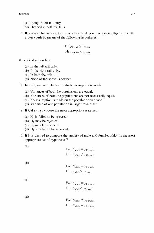
(c) Lying in left tail only
(d) Divided in both the tails
6. If a researcher wishes to test whether rural youth is less intelligent than the
urban youth by means of the following hypotheses,
H0 : mRural � mUrbanH1 : mRural<mUrban
the critical region lies
(a) In the left tail only.
(b) In the right tail only.
(c) In both the tails.
(d) None of the above is correct.
7. In using two-sample t-test, which assumption is used?
(a) Variances of both the populations are equal.
(b) Variances of both the populations are not necessarily equal.
(c) No assumption is made on the population variance.
(d) Variance of one population is larger than other.
8. If Cal t < ta, choose the most appropriate statement.
(a) H0 is failed to be rejected.
(b) H1 may be rejected.
(c) H0 may be rejected.
(d) H1 is failed to be accepted.
9. If it is desired to compare the anxiety of male and female, which is the most
appropriate set of hypotheses?
(a)H0 : mMale ¼ mFemale
H1 : mMale 6¼ mFemale
(b)H0 : mMale ¼ mFemale
H1 : mMale>mFemale
(c)H0 : mMale ¼ mFemale
H1 : mMale<mFemale
(d)H0 : mMale 6¼ mFemale
H1 : mMale ¼ mFemale
Exercise 217

10. In testing the following set of hypotheses,
H0 : m1 � m2H1 : m1<m2
choose the most appropriate statement.
(a) If Cal t � ta, H0 may not be rejected.
(b) If Cal t < �ta, H0 may be rejected.
(c) If Cal t > �ta, H0 may be rejected.
(d) None of the above is correct.
11. If there are N pairs of score and paired t-test is used for comparing the means of
both the groups, what will be the degrees of freedom for t-statistic?
(a) N(b) 2N � 2
(c) N + 1
(d) N � 1
12. If attitude toward science is to be compared among 22 male and 18 women
students of class XII by using t-ratio, what would be its degrees of freedom?
(a) 40
(b) 39
(c) 2
(d) 38
13. To see the effectiveness of observation method on learning skill, which of the
SPSS command shall be used?
(a) One-sample t-test(b) Independent-sample t-test(c) Paired-sample t-test(d) None of the above
14. Power of statistical test is given by
(a) b(b) 1 + b(c) b � 1
(d) 1 � b
Assignments
1. A random sample of 25 management students was tested for their IQ in a
university. Their scores were as follows:
92, 101, 94, 93, 97, 98, 120, 104, 98, 96, 85, 121, 87, 96, 111, 102, 99, 95, 89,
102, 131, 107, 109, 99, 97
Can it be concluded that the management students in the university have a mean
IQ score equal to 101? Test your hypothesis at 5% level.
218 6 Hypothesis Testing for Decision-Making

2. The following data set represents the weight of the average daily household
waste (kg/day/house) generated from 20 houses in a locality:
4.1 3.7 4.3 2.5 2.5 6.8 4.0 4.5 4.6 7.1
3.5 3.1 6.6 5.5 6.5 4.1 4.2 4.8 5.1 4.8
Can it be concluded that the average daily household waste of that community is
5.0 kg/day/house? Test your hypothesis at 1% level.
3. A feeding experiment was conducted with two random samples of pigs on the
relative value of limestone and bone meal for bone development. The data so
obtained on ash content are shown in the following table:
Test the significance of the difference between the mean ash content of the two
groups at 5% level.
4. A company wanted to know as to which of the two pizza types, that is, fresh
veggie and peppy paneer, was most popular among the people. An experiment
was conducted in which 12 men were given two types of pizza, that is, fresh
veggie pizza and pepper paneer pizza, to eat on two different days. Each pizza
was carefully weighed at exactly 16 oz. After 20 min, the leftover pizzas were
weighed, and the amount of each type of pizza remaining per person was
calculated assuming that the subjects would eat more if they preferred the
pizza type. The data so obtained is shown in the following table.
Ash contents (%) in the bones
of pigsS.N. Lime stone Bone stone
1 48.9 52.5
2 52.3 53.9
3 51.4 53.2
4 50.6 49.9
5 52 51.6
6 45.8 48.5
7 50.5 52.6
8 52.1 44.6
9 53 52.8
10 46.5 48.8
Weights of the leftover pizzas
in both varietiesS.N. Fresh veggie (in oz.) Pepper paneer (in oz.)
1 12.5 15
2 5.87 7.1
3 14 14
4 12.3 13.7
5 3.5 14.2
6 2.6 5.6
7 14.4 15.4
8 10.2 11.3
9 4.5 15.6
10 6.5 10.5
11 4.3 8.5
12 8.4 9.3
Exercise 219

Apply the paired t-test and interpret your findings. Do people seem to prefer
fresh veggie pizza over pepper veggie pizza? Test your hypothesis at 5% level.
Answers to Multiple-Choice Questions
Q.1 b Q.2 d
Q.3 c Q.4 c
Q.5 d Q.6 a
Q.7 a Q.8 a
Q.9 a Q.10 b
Q.11 d Q.12 d
Q.13 c Q.14 d
Assignments
1. Calculated value of t ¼ �0.037; average IQ score of the students is 101.
2. Calculated value of t ¼ �1.286; average daily household waste of the commu-
nity is 5 kg/day/house.
3. Calculated value of t ¼ �0.441; mean ash contents of both the groups are same.
4. Calculated value of t ¼ 3.193 which is significant. People prefer fresh veggie
pizza.
220 6 Hypothesis Testing for Decision-Making
Chapter 7
One-Way ANOVA: Comparing Means of More
than Two Samples
Learning Objectives
After completing this chapter, you should be able to do the following:
• Understand the basics of one-way analysis of variance (ANOVA).
• Learn to interpret the model involved in one-way analysis of variance.
• Learn the different designs of ANOVA.
• Describe the situations in which one-way analysis of variance should be used.
• Learn the manual procedure of applying one-way ANOVA in testing of
hypothesis.
• Construct the null and research hypotheses to be tested in the research study.
• Learn what happens if multiple t-tests are used instead of one-way ANOVA.
• Understand the steps involved in one-way analysis of variance in equal and
unequal sample sizes.
• Interpret the significance of F-statistic using the concept of p value.
• Know the procedure of making data file for analysis in SPSS.
• Understand the steps involved in using SPSS for solving the problems of one-
way analysis of variance.
• Describe the output of one-way analysis of variance obtained in SPSS.
Introduction
One-way analysis of variance is a statistical technique used for comparing means of
more than two groups. It tests the null hypothesis that samples in different groups
have been drawn from the same population. It is abbreviated as one-way ANOVA.
This technique can be used in a situation where the data is measured either on
interval or ratio scale. In one-way ANOVA, group means are compared by com-
paring the variability between groups with that of variability within the groups. This
is done by computing an F-statistic. The F-value is computed by dividing the mean
sum of squares between the groups by the mean sum of squares within the groups.
J.P. Verma, Data Analysis in Management with SPSS Software,DOI 10.1007/978-81-322-0786-3_7, # Springer India 2013
221

As per the central limit theorem, if the groups are drawn from the same popula-
tion, the variance between the group means should be lower than the variance
within the groups. Thus, a higher ratio (F-value) indicates that the samples have
been drawn from different populations.
There are varieties of situations in which one-way analysis of variance can be
used to compare the means of more than two groups. Consider a study in which it is
required to compare the responses of the students belonging to north, south, west
and east regions towards liking of mess food in the university. If the quality of mess
food is rated on a scale of 1–10 (1 ¼ “I hate the food,” 10 ¼ “Best food ever”),
then the responses of the students belonging to different regions can be obtained in
the form of the interval scores. Here the independent variable would be the
student’s region having four different levels namely north, south, east and west
whereas the response of the students shall be the dependent variable. To achieve the
objective of the study the null hypothesis of no difference among the mean
responses of the four groups may be tested against the alternative hypothesis that
at least one group mean differs. If the null hypothesis is rejected, a post hoc test is
used to get the correct picture as to which group’s liking is the best.
Similarly a human resource manager may wish to determine whether the
achievement motivation differs among the employees in three different age
categories (<25, 26–35, and >35 years) after attending a training program. Here,
the independent variable is the employee’s age category, whereas the achievement
motivation is the dependent variable. In this case, it is desired to test whether the
data provide sufficient evidence to indicate that the mean achievement motivation
of any age category differs from other. The one-way ANOVA can be used to answer
this question.
Principles of ANOVA Experiment
There are three basic principles of design of experiments, that is, randomization,
replication, and local control. Out of these three, only randomization and replica-
tion need to be satisfied by the one-way ANOVA experiments. Randomization
refers to the random allocation of the treatment to experimental units. On the other
hand, replication refers to the application of each individual level of the factor to
multiple subjects. In other words, the experiment must be replicated in more than
one subject. In the above example several employees in each age group should be
selected in a random fashion in order to satisfy the principles of randomization and
replication. This facilitates in drawing the representative sample.
One-Way ANOVA
It is used to compare the means of more than two independent groups. In one-way
ANOVA, the effect of different levels of only one factor on the dependent variable
is investigated. Usually one-way ANOVA is used for more than two groups because
222 7 One-Way ANOVA: Comparing Means of More than Two Samples
two groups may be compared using t-test. In comparing two group means, the t and Fare related as F ¼ t2. In using one-way ANOVA, the experimenter is often interested
in investigating the effect of different treatments on some subjects. Which may be
people, animals, or plants, etc. For instance, obesity can be compared among the
employees of three different departments: marketing, production, and human
resource of an organization. Similarly anxiety of the employees can be compared
in three different units of an organization. Thus, one-way ANOVA has a wide
application in management sciences, humanities, and social sciences.
Factorial ANOVA
A factorial design is the one in which the effect of two factors on the dependent
variable is investigated. Here each factor may have several levels and each combi-
nation becomes a treatment. Usually factorial ANOVA is used to compare the main
effect of each factor as well as their interaction effects across the levels of other
factor on the criterion variable. But the situation may arise where each combination
of levels in two factors is treated as a single treatment and it is required to compare
the effect of these treatments on the dependent variable. In such situation one-way
ANOVA can be used to test the required hypothesis. Consider a situation where the
effect of different combination of duration and time on learning efficiency is to be
investigated. The duration of interest is 30 and 60 minutes and the subjects are
given training in the morning and evening sessions for a learning task. The four
combinations of treatments would be morning time with 30 minutes duration,
morning time with 60 minutes duration, evening time with 30 minutes duration
and evening time with 60 minutes duration. In this case neither the main effect nor
the interaction effects are of interest to the investigator rather just the combinations
of these levels form four levels of the independent treatment.
If the number of factors and their levels are large, then lots of experimental
groups need to be created which is practically not possible, and in that case
fractional factorial design is used. In this design, only important combinations are
studied.
Repeated Measure ANOVA
Repeated measure ANOVA is used when same subjects are given different
treatments at different time interval. In this design, same criterion variable is
measured many times on each subject. This design is known as repeated measure
design because repeated measures are taken at different time in order to see the
impact of time on changes in criterion variable. In some studies of repeated measure
design, same criterion variable is compared under two or more different conditions.
For example, in order to see the impact of temperature on memory retention, a
subject’s memory might be tested once in an air-conditioned atmosphere and
another time in a normal room temperature.
Principles of ANOVA Experiment 223
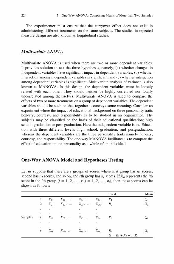
The experimenter must ensure that the carryover effect does not exist in
administering different treatments on the same subjects. The studies in repeated
measure design are also known as longitudinal studies.
Multivariate ANOVA
Multivariate ANOVA is used when there are two or more dependent variables.
It provides solution to test the three hypotheses, namely, (a) whether changes in
independent variables have significant impact in dependent variables, (b) whether
interaction among independent variables is significant, and (c) whether interaction
among dependent variables is significant. Multivariate analysis of variance is also
known as MANOVA. In this design, the dependent variables must be loosely
related with each other. They should neither be highly correlated nor totally
uncorrelated among themselves. Multivariate ANOVA is used to compare the
effects of two or more treatments on a group of dependent variables. The dependent
variables should be such so that together it conveys some meaning. Consider an
experiment where the impact of educational background on three personality traits
honesty, courtesy, and responsibility is to be studied in an organization. The
subjects may be classified on the basis of their educational qualification; high
school, graduation or post-graduation. Here the independent variable is the Educa-
tion with three different levels: high school, graduation, and postgraduation,
whereas the dependent variables are the three personality traits namely honesty,
courtesy, and responsibility. The one-way MANOVA facilitates us to compare the
effect of education on the personality as a whole of an individual.
One-Way ANOVA Model and Hypotheses Testing
Let us suppose that there are r groups of scores where first group has n1 scores,
second has n2 scores, and so on, and rth group has nr scores. If Xij represents the jthscore in the ith group (i ¼ 1, 2, . . ., r; j ¼ 1, 2, . . ., ni), then these scores can be
shown as follows:
Total Mean
1 X11 X12 . . ... X1j .... X1n1 R1 X1
2 X21 X22 . . ... X2j . . .. X2n2 R2 X2
. . . . .
. . . . .
Samples i Xi1 Xi2 . . ... Xij . . .. Xini Ri Xi
. . . . .
. . . . .
r Xr1 Xr2. . ... Xrj . . .. Xrnr Rr Xr
G ¼ R1 + R2 + . . .Rr
224 7 One-Way ANOVA: Comparing Means of More than Two Samples

Here,
N ¼ n1 + n2 + . . .nr, the total of all the scoresG is the grand total of all N scores
Ri is the total of all the scores in ith group
The total variability among the above-mentioned N scores can be attributed due
to the variability between groups and variability within groups. Thus, the total
variability can be broken into the following two components:
Total variability ¼ Variability between groupsþ Variability withinGroups
or TSS ¼ SSb þ SSw(7.1)
This is known as one-way ANOVA model where it is assumed that the variability
among the scores may be due to the groups. After developing the model, the
significance of the group variability is tested by comparing the variability between
groups with that of variability within groups by using the F-test.The null hypothesis which is being tested in this case is that whether variability
between groups (SSb) and variability within the groups (SSw) are the same or not.
If the null hypothesis is rejected, it is concluded that the variability due to groups is
significant, and it is inferred that means of all the groups are not same. On the other
hand, if the null hypothesis is not rejected, one may draw the inference that group
means do not differ significantly. Thus, if r groups are required to be compared on
some criterion variable, then the null hypothesis can be tested by following the
below mentioned steps:
(a) Hypothesis construction: The following null hypothesis is tested
H0 : m1 ¼ m2 ¼ . . . ¼ mr
against the alternative hypothesis that at least one mean differs.
(b) Level of significance: The level of significance may be chosen beforehand.
Usually it is taken as .05 or .01.
(c) Statistical test: The F-test is used to test the above mentioned hypothesis.
If F-value is significant, it indicates that the variability between groups is
significantly higher than the variability within groups; in that case, the null
hypothesis of no difference between the group means is rejected. F-value is
obtained by computing the total sum of squares (TSS), sum of squares between
groups (SSb), and sum of squares within groups (SSw):
(i) Total sum of squares (TSS): It indicates the variation present in the whole
data set around its mean value and is obtained by adding the sum of
squares due to “between groups” and sum of squares due to “within
groups.” The total sum of squares can be defined as the sum of squared
One-Way ANOVA Model and Hypotheses Testing 225
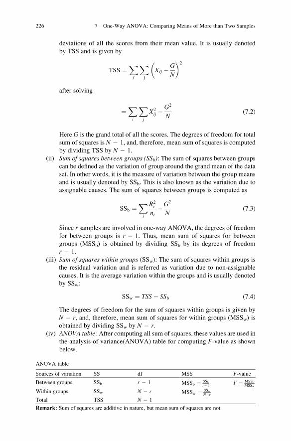
deviations of all the scores from their mean value. It is usually denoted
by TSS and is given by
TSS ¼Xi
Xj
Xij � G
N
� �2
after solving
¼Xi
Xj
X2ij �
G2
N(7.2)
Here G is the grand total of all the scores. The degrees of freedom for total
sum of squares is N � 1, and, therefore, mean sum of squares is computed
by dividing TSS by N � 1.
(ii) Sum of squares between groups (SSb): The sum of squares between groups
can be defined as the variation of group around the grand mean of the data
set. In other words, it is the measure of variation between the group means
and is usually denoted by SSb. This is also known as the variation due to
assignable causes. The sum of squares between groups is computed as
SSb ¼Xi
R2i
ni� G2
N(7.3)
Since r samples are involved in one-way ANOVA, the degrees of freedom
for between groups is r � 1. Thus, mean sum of squares for between
groups (MSSb) is obtained by dividing SSb by its degrees of freedom
r � 1.
(iii) Sum of squares within groups (SSw): The sum of squares within groups is
the residual variation and is referred as variation due to non-assignable
causes. It is the average variation within the groups and is usually denoted
by SSw:
SSw ¼ TSS� SSb (7.4)
The degrees of freedom for the sum of squares within groups is given by
N � r, and, therefore, mean sum of squares for within groups (MSSw) is
obtained by dividing SSw by N � r.(iv) ANOVA table:After computing all sum of squares, these values are used in
the analysis of variance(ANOVA) table for computing F-value as shown
below.
ANOVA table
Sources of variation SS df MSS F-value
Between groups SSb r � 1 MSSb ¼ SSbr�1
F ¼ MSSbMSSw
Within groups SSw N � r MSSw ¼ SSwN�r
Total TSS N � 1
Remark: Sum of squares are additive in nature, but mean sum of squares are not
226 7 One-Way ANOVA: Comparing Means of More than Two Samples

(v) F-statistic: Under the normality assumptions, the F-value obtained in the
above table, that is,
F ¼ MSSb
MSSw(7.5)
follows an F-distribution with (r � 1, N � r) degrees of freedom.
This test statistic F is used to test the null hypothesis of no difference among
the group means.
(d) Decision criteria: The tabulated value of F at .05 and .01 level of significance
with (r � 1, N � r) degrees of freedom may be obtained from Tables A.4 and
A.5, respectively, in the Appendix. If calculated value of F is greater than
tabulated F, the null hypothesis is rejected. And in that case it is concluded thatat least one of the means will be different. Since ANOVA does not tell us where
the difference lies, post hoc test is used to get the clear picture. There are several
post hoc tests which can be used, but least significant difference (LSD) test is
generally used in equal sample sizes, whereas Scheffe’s test is most often used
in unequal sample sizes.
In all the post hoc tests, a critical difference is calculated at a particular level
of significance, and if the difference of any pair of observed means is higher
than the critical difference, it is inferred that one mean is higher than the other;
otherwise, group means are equal. By comparing all pair of means, conclusion
is drawn as to which group mean is the highest. The procedure of such
comparison can be seen in the solved Example 7.1.
LSD test provides the critical difference (CD) which is used for comparing
differences in all the pair of means. The CD is computed as follows:
Critical difference ¼ t:05 N � rð Þ �ffiffiffiffiffiffiffiffiffiffiffiffiffiffiffiffiffiffiffiffi2
nMSSð Þw
r(7.6)
where the symbols have their usual meanings.
Since Scheffe’s test is used in case of unequal sample size hence it also provides
different critical difference for comparing different pair of group means. Here
the critical difference (CD) is calculated as follows:
CD for comparing ith and jth groupmeans
¼ffiffiffiffiffiffiffiffiffiffiffiffiffiffiffiffiffiffiffiffiffiffiffiffiffiffiffiffiffiffiffiffiffiffiffiffiffiffiffiffiffiffiffiffiffiffiffiffiffir � 1ð ÞF:05 r � 1;N � rð Þ
p�
ffiffiffiffiffiffiffiffiffiffiffiffiffiffiffiffiffiffiffiffiffiffiffiffiffiffiffiffiffiffiffiffiffiMSSw
1
niþ 1
nj
� �s(7.7)
where ni and nj represent the sample sizes of ith and jth groups, respectively,
and other symbols have their usual meanings.
The SPSS output provides p value (significant value) for each pair of means
to test the significance of difference between them. If p value for any pair
One-Way ANOVA Model and Hypotheses Testing 227

of means is less than .05, it is concluded that means are significantly different
otherwise not. SPSS provides various options for post hoc tests. One may
choose one or more options for analysis while using SPSS.
Assumptions in Using One-Way ANOVA
While applying one-way ANOVA for comparing means of different groups, the
following assumptions are made:
1. The data must be measured either on interval or ratio scale.
2. The samples must be independent.
3. The dependent variable must be normally distributed.
4. The population from which the samples have been drawn must be normally
distributed.
5. The variances of the population must be equal.
6. The errors are independent and normally distributed.
Remarks
1. ANOVA is a relatively robust procedure in case of violations of the normality
assumption.
2. In case the data is ordinal, a nonparametric alternative such as Kruskal-Wallis
one-way analysis of variance should be used instead of parametric one-way
ANOVA.
Effect of Using Several t-tests Instead of ANOVA
Many times a researcher argues that what if I use three t-tests rather than using
one-way ANOVA in comparing the means of three groups. One of the logics is that,
why to use three times t-test if equality of means can be tested by using one-way
ANOVA once. If the number of groups are more, then one needs to apply large
number of t-tests. For example, in case of six groups, one needs to apply 6C2 ¼ 15,
t-tests instead of one-time one-way ANOVA. This may be one of the arguments of
the researcher in favor of using one-way ANOVA, but the main problem in using
multiple t-tests instead of one-way ANOVA is that the type I error gets inflated.
If the level of significance has been chosen as p1, then Fisher has showed that thetype I error rate expands from p1 to some larger value as the number of tests
between paired means increases. The error rate expansion is constant and predict-
able which can be computed by the following equation:
p ¼ 1� 1� p1ð Þr (7.8)
where p is the new level of significance and r is the number of t-tests used for
comparing all the pair of group means.
228 7 One-Way ANOVA: Comparing Means of More than Two Samples

For example, in comparing three group means, if t-tests are used instead of one-
way ANOVA and if the level of significance is chosen as .05, then the total number
of paired comparison would be 3C2 ¼ 3.
Here, p1 ¼ 0.05 and r ¼ 3, and, therefore, the actual level of significance
becomes
p ¼ 1� ð1� p1Þr
¼ 1� 1� 0:5ð Þ3 ¼ 1� 0:953 ¼ 1� 0:8574
¼ 0:143
Thus, in comparing three group means instead of using one-way ANOVA, if
three t-tests are applied, then level of significance shall inflate from .05 to 0.143.
Application of One-Way ANOVA
One-way ANOVA is used when more than two group means are compared. Such
situations are very frequent in management research where a researcher may like to
compare more than two group means. For instance, one may like to compare the
mood state of the employees working in three different plants or to compare the
occupational stress among three different age categories of employees in an
organization.
Consider an experiment where a market analyst of a company is interested to
know the effect of three different types of incentives on the sale of a particular brand
of shampoo. Shampoo is sold to the customers with three schemes. In the first scheme
20% extra is offered in the same price, in the second scheme shampoo is sold with
free bath soap, whereas in the third scheme it is sold to the customers with a free
ladies’ perfume. These three schemes are offered to the customers in the same outlet
for 3 months. During the second month, sales of the shampoo are recorded in all three
schemes for 20 days. In this situation, scheme is the independent variable having
three different levels: 20% extra shampoo, shampoo with a bath soap, and shampoo
with a ladies’ perfume whereas, the sales figure is the dependent variable. Here the
null hypothesis which is required to be tested would be
H0 : Average sale of shampoo in all three incentive groups are same against the
alternative hypothesis.
H1 : At least one group mean is different.
The one-way ANOVA may be applied to compute F-value. If F-statistic is
significant, the null hypothesis may be rejected, and in that case, a post hoc test
may be applied to find as to which incentive is the most attractive in improving the
sale of the shampoo. On the other hand, if F-value is not significant, one fails to
reject the null hypothesis, and in that case, there would be no reason to believe that
any one incentive is better than others to enhance the sale.
Application of One-Way ANOVA 229

Example 7.1 An audio company predicts that students learn more effectively with
a constant low-tune melodious music in background, as opposed to an irregular loud
orchestra or no music at all. To verify this hypothesis, a study was planned by
dividing 30 students into three groups of ten each. Students were assigned to these
three groups in a random fashion, and all of them were given a comprehension to
read for 20 min. Students in group 1 were asked to study the comprehension with
low-tune melodious music at a constant volume in the background. Whereas the
students in group 2 were exposed to loud orchestra and group 3 to no music at all
while reading the comprehension. After reading the comprehension, they were
asked to solve few questions. The marks obtained are shown in the Table 7.1.
Do these data confirm that learning is more effective in particular background
music? Test your hypothesis at 5% level.
Solution Following steps shall be taken to test the required hypothesis:
(a) Hypotheses construction: The researcher is interested in testing the following
null hypothesis:
H0 : mMusic ¼ mOrchestra ¼ mWithout Music
against the alternative hypothesis that at least one mean is different.
(b) Level of significance: 0.05(c) Statistical test: One-way ANOVA shall be used to test the null hypothesis. In
order to complete the ANOVA table, first, all the sum of squares are computed.
Here,
Number of groups ¼ r ¼ 3
Sample size in each group ¼ n ¼ 10
Total number of scores ¼ nr ¼ 30
The computation of group total, group means, and grand total has to be
computed first which is shown in Table 7.2.
(i) Correction factor CFð Þ ¼ G2
N¼ 1352
30¼ 607:5
ðiiÞ Raw sum of squares RSSð Þ ¼Xi
Xj
X2ij
¼ 82 þ 42 þ 82 þ . . . 92 þ 62� �þ 42 þ 62 þ 32 þ . . . 42 þ 32� �
þ 32 þ 42 þ 62 þ . . . 12 þ 22� �
¼ 440þ 188þ 127 ¼ 755
230 7 One-Way ANOVA: Comparing Means of More than Two Samples
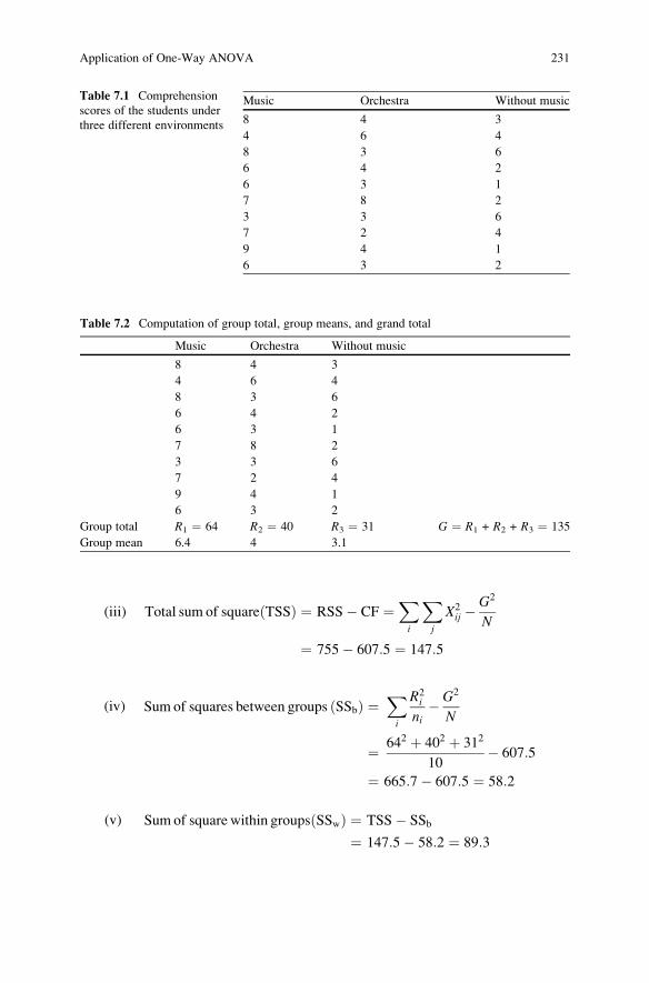
(iii) Total sum of square TSSð Þ ¼ RSS� CF ¼Xi
Xj
X2ij �
G2
N
¼ 755� 607:5 ¼ 147:5
(iv) Sum of squares between groups SSbð Þ ¼Xi
R2i
ni� G2
N
¼ 642 þ 402 þ 312
10� 607:5
¼ 665:7� 607:5 ¼ 58:2
(v) Sumof squarewithin groups SSwð Þ ¼ TSS� SSb
¼ 147:5� 58:2 ¼ 89:3
Table 7.2 Computation of group total, group means, and grand total
Music Orchestra Without music
8 4 3
4 6 4
8 3 6
6 4 2
6 3 1
7 8 2
3 3 6
7 2 4
9 4 1
6 3 2
Group total R1 ¼ 64 R2 ¼ 40 R3 ¼ 31 G ¼ R1 + R2 + R3 ¼ 135
Group mean 6.4 4 3.1
Table 7.1 Comprehension
scores of the students under
three different environments
Music Orchestra Without music
8 4 3
4 6 4
8 3 6
6 4 2
6 3 1
7 8 2
3 3 6
7 2 4
9 4 1
6 3 2
Application of One-Way ANOVA 231

(d) Decision criteriaFrom Table A.4 in the Appendix, F.05(2,27) ¼ 4.22.
Since calculated F(¼8.79) > F.05(2,27), the null hypothesis may be rejected.
It is therefore concluded that learning efficiency in all the three experimental
groups is not same. In order to find as to which group’s learning efficiency is
best, the least significance difference (LSD) test shall be applied. The critical
difference in LSD test is given by
CD ¼ t:05 27ð Þ �ffiffiffiffiffiffiffiffiffiffiffiffiffiffiffiffiffiffiffiffiffi2�MSSw
n
r
¼ 2:052�ffiffiffiffiffiffiffiffiffiffiffiffiffiffiffiffiffi2� 3:31
10
r¼ 1:67
(e) ResultsThe group means may be compared by arranging them in descending order as
shown in the Table 7.4
It is clear from Table 7.4 that the mean difference between “music” and
“orchestra” groups as well as “music” and “without music” groups is greater
than the critical difference. Since the mean difference between orchestra and
without music groups is significant hence it is shown by clubbing their means
by the line as shown in the Table 7.4.
(f) InferenceFrom the results, it is clear that the mean learning performance in music group
is significantly higher than that of orchestra as well as nonmusic groups,
whereas the mean learning of orchestra group is equal to that of nonmusic
group. It is therefore concluded that melodious music improves the learning
efficiency.
Table 7.3 ANOVA table for the data on comprehension test
Sources of variation SS df MSS F-value
Between groups 58.2 r � 1 ¼ 2 58:22
¼ 29:1
8.79
Within groups 89.3 N � r ¼ 27 89:327
¼ 3:31
Total 147.5 N � 1 ¼ 29
Table 7.4 Group means and their comparison
Music Orchestra Without music CD at 5% level
6.4 4 3.1 1.67
“ ” represents no significant difference between
the means at 5% level
232 7 One-Way ANOVA: Comparing Means of More than Two Samples

Solved Example of One-Way ANOVA with Equal Sample Size
Using SPSS
Example 7.2 The data in the following table indicates the psychological health
ratings of corporate executives in banking, insurance, and retail sectors. Apply one-
way ANOVA to test whether the executives of any particular sector are healthier in
their psychological health in comparison to other sectors. Test your hypothesis at
5% as well as 1% level (Table 7.5).
Solution
In this problem, it is required to test the following null hypothesis
H0 : mBanking ¼ mInsurance ¼ mRetail
against the alternative hypothesis that at least one mean differs.
The SPSS output provides F-value along with its significance value (p value).
The F-value would be significant if the p value is less than .05. If F-value becomes
significant, a post hoc test shall be used to compare the paired means. SPSS
provides facility to choose one or more post hoc test for analysis.
In this example, since the sample sizes are equal, LSD test shall be used as a
post hoc test for comparing the group means. However, one can choose other post
hoc tests as well. The SPSS output provides the p value for testing the significanceof the difference between each pair of group means. Thus, by looking to the
results of post hoc test, one can determine as to which group mean is higher. The
procedure has been discussed while interpreting the output.
Table 7.5 Data on
psychological healthS.N. Banking Insurance Retail
1 45 41 58
2 41 38 54
3 47 43 49
4 59 53 65
5 48 43 51
6 45 42 56
7 38 40 41
8 48 42 51
9 39 32 45
10 42 39 53
11 38 36 37
12 36 32 42
13 45 40 44
14 38 39 32
15 42 40 50
Solved Example of One-Way ANOVA with Equal Sample Size Using SPSS 233

Computations in One-Way ANOVA with Equal Sample Size
(a) Preparing data fileA data file needs to be prepared before using the SPSS commands for one-way
ANOVA with equal samples size. The following steps will help you prepare the
data file:
(i) Starting the SPSS: Use the following command sequence to start SPSS:
Start ! Programs ! IBM SPSS Statistics ! IBM SPSS Statistics 20
After clicking the Type in Data, you will be taken to the Variable View
option for defining the variables in the study.
(ii) Defining variables: There are two variables in this example which need to
be defined along with their properties while preparing the data file. These
variables are psychological health and sector. The psychological health is
defined as scale variable, whereas sector is defined as nominal variable as
they are measured on interval as well as nominal scales, respectively. The
procedure of defining these variables in the SPSS is as follows:
1. Click the Variable View to define the variables and their properties.
2. Write short name of the variables as Psy_Health and Sector under thecolumn heading Name.
3. Under the column heading Label, full names of these variables have
been defined as Psychological health rating and Different sector,respectively. You may choose some other names of these variables
as well.
4. For the variable Sector, double-click the cell under the column
heading Values and add the following values to different levels:
Value Label
1 Banking
2 Insurance
3 Retail
5. Under the column headingMeasure, select the option “Scale” for the
Psy_Health variable and “Nominal” for the Sector variable.6. Use default entries in rest of the columns. The screen shall look like
Fig. 7.1.
Remark: Many variables can be defined in the variable view simulta-
neously if ANOVA is to be applied for more than one variable.
(iii) Entering dataAfter defining both the variables in Variable View, click Data View on
the left corner in the bottom of the screen as shown in Fig. 7.1 to open the
234 7 One-Way ANOVA: Comparing Means of More than Two Samples

data entry format column wise. After entering the data, the screen will look
like as shown in Fig. 7.2. Since the data is large, only a portion of data is
shown in the figure. Save the data file in the desired location before further
processing.
(b) SPSS commands for one-way ANOVAAfter entering all the data in the data view, follow the below-mentioned steps
for one-way analysis of variance:
(i) Initiating the SPSS commands for one-way ANOVA: In data view, click the
following commands in sequence:
Analyze ➾ Compare Means ➾ One-Way ANOVA
The screen shall look like Fig. 7.3.
(ii) Selecting variables for one-way ANOVA: After clicking the One-Way
ANOVA option, you will be taken to the next screen for selecting
variables. Select the variables Psychological health rating and Differentsector from left panel to the “Dependent list” section and “Factor” section
of the right panel, respectively. The screen will look like Fig. 7.4.
(iii) Selecting the options for computation: After selecting the variables, optionneeds to be defined for generating the output in one-way ANOVA. Take
the following steps:
– Click the tag Post Hoc in the screen shown in Fig. 7.4.
– Check theoption “LSD.”LSD test is selectedbecause the sample sizes
are equal. You may choose any other post hoc test if you so desire.
– Write “Significance level” as .05. By default, it is selected. However,
you may select any other significance level like .01 or .10 as well.
– Click Continue.
Fig. 7.1 Defining variables along with their characteristics
Solved Example of One-Way ANOVA with Equal Sample Size Using SPSS 235

The screen will look like Fig. 7.5.
– Click the tag Options in the screen shown in Fig. 7.4 and then check
‘Descriptive’.
– Click Continue.
The screen for this option shall look like Fig. 7.6.
– After selecting the options, the screen shown in Fig. 7.4 shall be
restored.
– Click OK.
Fig. 7.2 Screen showing
entered data for the
psychological health and
sector in the data view
236 7 One-Way ANOVA: Comparing Means of More than Two Samples

Fig. 7.3 Screen showing SPSS commands for one-way ANOVA
Fig. 7.4 Screen showing selection of variables for one-way ANOVA
Solved Example of One-Way ANOVA with Equal Sample Size Using SPSS 237

(c) Getting the outputAfter clickingOK in the screen shown in Fig. 7.4, the output shall be generated
in the output window. The relevant outputs may be selected by using right click
of the mouse and may be copied in the word file. Here, the following outputs
shall be generated:
1. Descriptive statistics
2. ANOVA table
3. Post hoc comparison table
In this example, all the outputs so generated by the SPSS will look like as shown
in Tables 7.6, 7.7, and 7.8.
Interpretations of the Outputs
Different descriptive statistics have been shown in Table 7.6 which may be used to
study the nature of the data. Further descriptive profiles of the psychological health
rating for the corporate executives in different sectors can be developed by using
the values of mean, standard deviation, and minimum and maximum scores in each
groups. The procedure of developing such profile has been discussed in Chap. 2 of
this book.
Fig. 7.5 Screen showing options for post hoc test and significance level
238 7 One-Way ANOVA: Comparing Means of More than Two Samples
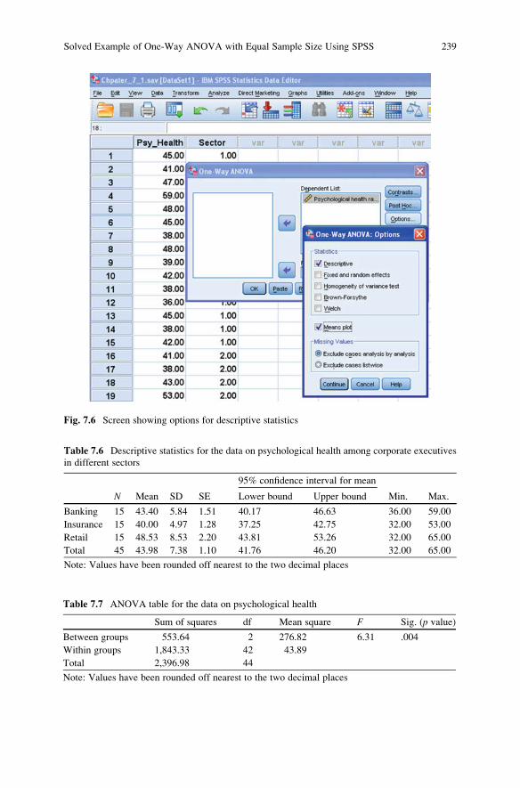
Table 7.6 Descriptive statistics for the data on psychological health among corporate executives
in different sectors
95% confidence interval for mean
N Mean SD SE Lower bound Upper bound Min. Max.
Banking 15 43.40 5.84 1.51 40.17 46.63 36.00 59.00
Insurance 15 40.00 4.97 1.28 37.25 42.75 32.00 53.00
Retail 15 48.53 8.53 2.20 43.81 53.26 32.00 65.00
Total 45 43.98 7.38 1.10 41.76 46.20 32.00 65.00
Note: Values have been rounded off nearest to the two decimal places
Table 7.7 ANOVA table for the data on psychological health
Sum of squares df Mean square F Sig. (p value)
Between groups 553.64 2 276.82 6.31 .004
Within groups 1,843.33 42 43.89
Total 2,396.98 44
Note: Values have been rounded off nearest to the two decimal places
Fig. 7.6 Screen showing options for descriptive statistics
Solved Example of One-Way ANOVA with Equal Sample Size Using SPSS 239

The mean of different groups in Table 7.6 and the results of Table 7.8 have been
used to prepare the graphics shown in Table 7.9 which can be used to draw
conclusions about post hoc comparison of means.
The F-value in Table 7.7 is significant at 5% level because its p value (¼.004) is
less than .05. Thus, the null hypothesis of no difference among the means of the
three groups may be rejected at 5% level. Since the p value is also less than .01, thenull hypothesis may be rejected at 1% level also.
Here, the F-value is significant; hence, the post hoc test needs to be applied for
testing the significance of mean difference between different pairs of groups.
Table 7.8 provides such comparison. It can be seen from this table that the
difference between banking and retail groups on their psychological health rating
is significant at 5% level because the p value for this mean difference is .04 which is
less than .05.
Similarly, the difference between insurance and retail groups on their psycho-
logical health is also significant at 5% as well as 1% level because the p value
attached to this mean difference is .001 which is less than .05 as well as .01.
There is no significant difference between the banking and insurance groups on
their psychological health rating because the p value attached to this group is .167
which is more than .05.
All the above-mentioned three findings can be very easily understood by looking
to the graphics in Table 7.9. From this table, it is clear that the mean psychological
health rating score is highest among the executives in the retail sector in comparison
to that of banking and insurance sectors. It may thus be concluded that the psycho-
logical health of the executives in the retail sector is best in comparison to that of
banking and insurance sectors.
Table 7.8 Post hoc comparison of means using LSD test
(I) Different sectors (J) Different sectors Mean difference (I � J) Std. error Sig. (p value)
Banking Insurance 3.40 2.42 .167
Retail �5.13* 2.42 .040
Insurance Banking �3.40 2.42 .167
Retail �8.53** 2.42 .001
Retail Banking 5.13* 2.42 .040
Insurance 8.53** 2.42 .001
Note: The values of lower bound and upper bound have been omitted from the original output. The
values have been rounded off nearest to the two decimal places
*The mean difference is significant at 5% level
**The mean difference is significant at 1% level
Table 7.9 Mean scores on
psychological health in
different groups
Retail Banking Insurance
48.53 43.40 40.00
“ ” represents no significant differ-
ence between the means
240 7 One-Way ANOVA: Comparing Means of More than Two Samples

Solved Example of One-Way ANOVA with Unequal Sample
Example 7.3 A human resource department of an organization conducted a study
to know the status of occupational stress among their employees in different age
categories. A questionnaire was used to assess the stress level of the employees in
three different age categories: <40, 40–55, and >55 years. The stress scores so
obtained are shown in Table 7.10.
Apply one-way analysis of variance to test whether mean stress score of the
employees in any two age categories are different. Test your hypothesis at 5% level.
Solution Solving problems of one-way ANOVA with equal and unequal samples
through SPSS are almost similar. In case of unequal sample size, one should be
careful in feeding the data. The procedure of feeding the data in this case shall be
discussed below. Here, the SPSS procedure shall be discussed in brief as it is
exactly similar to the one discussed in Example 7.2. Readers are advised to refer
to the procedure mentioned in Example 7.2 in case of doubt in solving this problem
of unequal sample size.
Here, the null hypothesis which needs to be tested is
H0 : mA ¼ mB ¼ mC
against the alternative hypothesis that at least one group mean differs.
If the null hypothesis is rejected, post hoc test will be used for comparing group
means. Since the sample sizes are different, the Scheffe’s test has been used for post
hoc analysis.
Table 7.10 Occupational stress scores among the employees in different age categories
Group A (<40 years) Group B (40–55 years) Group C (>55 years)
54 75 55
48 68 51
47 68 59
54 71 64
56 79 52
62 86 48
56 81 65
45 79 48
51 72 56
54 78 49
48 69
52
Solved Example of One-Way ANOVA with Unequal Sample 241

Computations in One-Way ANOVA with Unequal Sample Size
(a) Preparing data file:
(i) Starting the SPSS: Start the SPSS the way it has been done in the above-
mentioned example and click the Type in Data option. You will be taken
to the Variable View option for defining the variables in the study.
(ii) Defining variables: There are two variables in this example that need to be
defined along with their properties while preparing the data file. The two
variables are stress scores and age group. The stress score is defined as
scale variable, whereas age group is defined as nominal variable as they
are measured on interval as well as nominal scales, respectively. The
procedure of defining these variables in the SPSS is as follows:
1. Click Variable View to define variables and their properties.
2. Write short name of the variables as Stress and Age_Gp under the
column heading Name.
3. Under the column heading Label, full names of these variables may
be defined as Stress scores and Age group, respectively. You may
choose some other names of these variables as well.
4. For the variable Age group, double-click the cell under the column
heading Values and add the following values to different levels:
Value Label
1 Group A (<40 years)
2 Group B (40–55 years)
3 Group C (>55 years)
5. Under the column headingMeasure, select the option “Scale” for the
Stress variable and “Nominal” for the Age_Gp variable.
6. Use default entries in rest of the columns.
After defining all the variables in variable view, the screen shall look like
Fig. 7.7.
Remark: More than one variable can be defined in the variable view for
doing ANOVA for many variables simultaneously.
(iii) Entering the data: After defining the variables in the Variable View, enterthe data, column-wise in Data View. The data feeding shall be done as
follows:
242 7 One-Way ANOVA: Comparing Means of More than Two Samples

Format of data feeding in Data View
S.N. Stress Age_Gp
Group A n1 =12
1 54 1
2 48 1
3 47 1
4 54 1
5 56 1
6 62 1
7 56 1
8 45 1
9 51 1
10 54 1
11 48 1
12 52 1
Group B n2 = 11
13 75 2
14 68 2
15 68 2
16 71 2
17 79 2
18 86 2
19 81 2
20 79 2
21 72 2
22 78 2
23 69 2
Group C n3 = 10
24 55 3
25 51 3
26 59 3
27 64 3
28 52 3
29 48 3
30 65 3
31 48 3
32 56 3
33 49 3
After feeding the data as mentioned above, the final screen shall look like Fig. 7.8.
(b) SPSS commands for one-way ANOVA for unequal sample sizeAfter entering all the data in data view, save the data file in the desired location
before further processing.
(i) Initiating the SPSS commands for one-way ANOVA: In data view, go to the
following commands in sequence:
Analyze ➾ Compare Means ➾ One-Way ANOVA
(ii) Selecting variables for analysis: After clicking the One-Way ANOVA
option, you will be taken to the next screen for selecting variables. Select
Solved Example of One-Way ANOVA with Unequal Sample 243
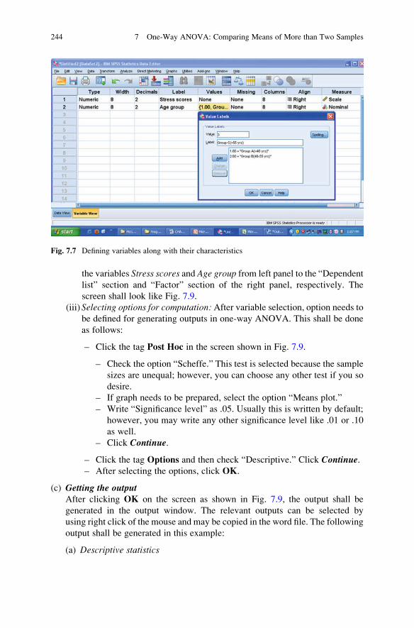
the variables Stress scores and Age group from left panel to the “Dependent
list” section and “Factor” section of the right panel, respectively. The
screen shall look like Fig. 7.9.
(iii)Selecting options for computation: After variable selection, option needs tobe defined for generating outputs in one-way ANOVA. This shall be done
as follows:
– Click the tag Post Hoc in the screen shown in Fig. 7.9.
– Check the option “Scheffe.” This test is selected because the sample
sizes are unequal; however, you can choose any other test if you so
desire.
– If graph needs to be prepared, select the option “Means plot.”
– Write “Significance level” as .05. Usually this is written by default;
however, you may write any other significance level like .01 or .10
as well.
– Click Continue.
– Click the tag Options and then check “Descriptive.” Click Continue.– After selecting the options, click OK.
(c) Getting the outputAfter clicking OK on the screen as shown in Fig. 7.9, the output shall be
generated in the output window. The relevant outputs can be selected by
using right click of the mouse and may be copied in the word file. The following
output shall be generated in this example:
(a) Descriptive statistics
Fig. 7.7 Defining variables along with their characteristics
244 7 One-Way ANOVA: Comparing Means of More than Two Samples

(b) ANOVA table(c) Post hoc comparison table(d) Graph for means plot
These outputs are shown in Tables 7.11, 7.12, and 7.13 and in Fig. 7.10. The
Table 7.14 has been developed by using the descriptive statistics from the
Table 7.11 and inputs from Table 7.13.
Fig. 7.8 Showing data entry
of stress scores for the
employees in different age
categories in data view
Solved Example of One-Way ANOVA with Unequal Sample 245

Interpretation of the Outputs
Table 7.11 shows the descriptive statistics of the data on occupational stress of
employees in different age categories. These statistics can be used to develop a
graphic profile of the employee’s occupational stress in different age categories.
Fig. 7.9 Screen showing selection of variables
Table 7.11 Descriptive statistics for the data on occupational stress of employees in different age
categories
95% confidence interval for mean
N Mean SD SE Lower bound Upper bound Min. Max.
Group A (<40 years) 12 52.25 4.77 1.38 49.23 55.28 45.00 62.00
Group B
(40–55 years)
11 75.09 5.97 1.80 71.08 79.10 68.00 86.00
Group C (>55 years) 10 54.70 6.29 1.99 50.20 59.20 48.00 65.00
Total 33 60.61 11.80 2.05 56.42 64.79 45.00 86.00
Table 7.12 ANOVA table for the data on occupational stress
Sum of squares df Mean square F Sig.
Between groups 3494.620 2 1747.310 54.42 .000
Within groups 963.259 30 32.109
Total 4457.879 32
246 7 One-Way ANOVA: Comparing Means of More than Two Samples

The procedure of developing such profile has been discussed in detail in Chap. 2 of
this book. Further, these descriptive statistics can be used to discuss the nature of
data in different age categories.
Table 7.12 gives the value of calculated F. The p value attached with the F is
.000 which is less than .05 as well as .01; hence, it is significant at 5% as well as 1%
levels. Since the F-value is significant, the null hypothesis of no difference in the
occupational stress among the employees in all the three age categories is rejected.
The post hoc test is now used to compare the means in different pairs.
SPSS provides the option of choosing the post hoc test, and, therefore, one may
choose any one or more test for post hoc analysis. In this example, the Scheffe’s test
was chosen to compare the means in different pairs. Table 7.13 provides such
comparisons.
It can be seen that the difference between occupational stress of the employees in
group A (<40 years) and group B (40–55 years) is significant at 5% as well as at 1%
level both as the p value for this mean difference is .000 which is less than .05 as
well as .01. Similarly, the mean difference between occupational stress of the
employees in group B (40–55 years) and group C (>55 years) is also significant
at 5% as well as 1% level both as the p value for this mean difference is .000 which
is also less than .05 and .01. However, there is no significant difference between the
occupational stress of the employees in group A (<40 years) and group C
(>55 years) because the p value is .606.
Fig. 7.10 Graphical presentation of mean scores of occupational stress in three different age
categories
Solved Example of One-Way ANOVA with Unequal Sample 247

The above results can be easily understood by looking to the graphics in
Table 7.14. This table has been obtained by combining the results of Tables 7.11
and 7.13.
Table 7.14 reveals that the mean occupational stress is highest among the
employees in group B (40–55 years). Further, mean occupation stress is similar in
group C (>55 years) and group A (<40 years). Since the option for mean plot was
selected in the SPSS, Fig. 7.10 has been generated in the output which shows the
mean plots of all the groups. The graph provides the conclusion at a glance.
Inference: On the basis of the results obtained above, it may be inferred that the
occupational stress among the employees in the age category 40–55 years is
maximum. The researcher may write their own reasons for these findings after
studying the lifestyle and working environment of the employees in this age
category. The results in the study provide an opportunity to the researcher to
write their own reasoning or develop their theoretical concepts supported by the
review of literatures.
Summary of the SPSS Commands for One-Way ANOVA
(Example 7.2)
(i) Start the SPSS by using the following commands:
Start ! Programs ! IBM SPSS Statistics ! IBM SPSS Statistics 20
(ii) Click Variable View tag and define the variables Psy_Health and Sector asscale and nominal variables, respectively.
Table 7.13 Post hoc comparison of group means using Scheffe’s test
(I) Age group (J) Age group Mean diff. (I � J) SE Sig. (p value)
Group A (<40 years) Group B (40–55 years) �22.84091* 2.36531 .000
Group C (>55 years) �2.45000 2.42623 .606
Group B (40–55 years) Group A (<40 years) 22.84091* 2.36531 .000
Group C (>55 years) 20.39091* 2.47585 .000
Group C (>55 years) Group A (<40 years) 2.45000 2.42623 .606
Group B (40–55 years) �20.39091* 2.47585 .000
Note: The values of lower bound and upper bound have been omitted from the original output
*The mean difference is significant at 5% as well as 1% levels
Table 7.14 Mean scores on occupational stress
in different groups
Group B
(40–55 years)
Group C
(>55 years)
Group A
(<40 years)
75.09 54.70 52.25
“ ” represents no significant difference
between the means
248 7 One-Way ANOVA: Comparing Means of More than Two Samples

(iii) Under the column heading Values, define “1” for banking, “2” for insur-
ance, and “3” for retail.
(iv) After defining variables, type the data for these variables by clicking Data
View.
(v) In the data view, follow the below-mentioned command sequence for the
computation involved in one-way analysis of variance:
Analyze ➾ Compare Means ➾ One-Way ANOVA
(vi) Select the variables Psychological health rating and Different sector fromleft panel to the “Dependent list” section and “Factor” section of the right
panel, respectively.
(vii) Click the tag Post Hoc and check the option “LSD” and ensure that the
value of “Significance level” is written as .05. Click Continue.(viii) Click the tag Options and then check “Descriptive.” Press Continue.(ix) Press OK for output.
Exercise
Short Answer Questions
Note: Write answer to each of the following questions in not more than 200 words.
Q.1. In an experiment, it is desired to compare the time taken to complete a task
by the employees in three age groups, namely, 20–30, 31–40, and
41–50 years. Write the null hypothesis as well as all possible types of
alternative hypotheses.
Q.2. Explain a situation where one-way analysis of variance can be applied.
Which variances are compared in one-way ANOVA?
Q.3. Define principles of ANOVA.What impact it will have if these principles are
not met?
Q.4. In what situations factorial experiments are planned? Discuss a specific
situation where it can be used.
Q.5. What is repeated measure design? What precaution one must take in framing
such an experiment?
Q.6. Discuss the procedure of one-way ANOVA in testing of hypotheses.
Q.7. Write a short note on post hoc tests.
Q.8. What do you mean by different sum of squares? Which sum of square you
would like to increase and decrease in your experiment and why?
Q.9. What are the assumptions in applying one-way ANOVA?
Q.10. If you use multiple t-tests instead of one-way ANOVA, what impact it will
have on results?
Q.11. Analysis of variance is used for comparing means of different groups, but in
doing so F-test is applied, which is a test of significance for comparing the
variances of two groups. Discuss this anomaly.
Exercise 249

Q.12. What do you mean by the post hoc test? Differentiate between LSD and
Scheffe’s test.
Q.13. What is p value? In what context it is used?
Multiple Choice Questions
Note: For each of the question, there are four alternative answers. Tick mark the one
that you consider the closest to the correct answer.
1. In one-way ANOVA experiment, which of the following is a randomization
assumption that must be true?
(a) The treatment must be randomly assigned to the subjects.
(b) Groups must be chosen randomly.
(c) The type of data can be randomly chosen to either categorical or quantitative.
(d) The treatments must be randomly assigned to the groups.
2. Choose the correct statement.
(a) Total sum of square is additive in nature.
(b) Total mean sum of square is additive in nature.
(c) Total sum of square is nonadditive.
(d) None of the above is correct.
3. In one-way ANOVA, Xij represents
(a) The sample mean of the criterion variable for the ith group
(b) The criterion variable value for the ith subject in the jth group
(c) The number of observations in the jth group
(d) The criterion variable value for the jth subject in the ith group
4. In one-way ANOVA, TSS measures
(a) The variability within groups
(b) The variability between groups
(c) The overall variability in the data
(d) The variability of the criterion variable in any group.
5. In an experiment, three unequal groups are compared with total number of
observations in all the groups as 31 (with some items missing). Calculate the
test statistic for one-way ANOVA F-test.
Source df SS MS F
Between groups 7.5 3.75 ?
Within groups
Total 20.8
250 7 One-Way ANOVA: Comparing Means of More than Two Samples
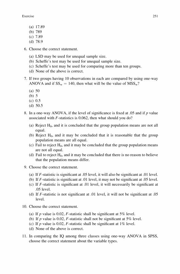
(a) 17.89
(b) 789
(c) 7.89
(d) 78.9
6. Choose the correct statement.
(a) LSD may be used for unequal sample size.
(b) Scheffe’s test may be used for unequal sample size.
(c) Scheffe’s test may be used for comparing more than ten groups.
(d) None of the above is correct.
7. If two groups having 10 observations in each are compared by using one-way
ANOVA and if SSw ¼ 140, then what will be the value of MSSw?
(a) 50
(b) 5
(c) 0.5
(d) 50.5
8. In a one-way ANOVA, if the level of significance is fixed at .05 and if p value
associated with F-statistics is 0.062, then what should you do?
(a) Reject H0, and it is concluded that the group population means are not all
equal.
(b) Reject H0, and it may be concluded that it is reasonable that the group
population means are all equal.
(c) Fail to reject H0, and it may be concluded that the group population means
are not all equal.
(d) Fail to reject H0, and it may be concluded that there is no reason to believe
that the population means differ.
9. Choose the correct statement.
(a) If F-statistic is significant at .05 level, it will also be significant at .01 level.(b) If F-statistic is significant at .01 level, it may not be significant at .05 level.
(c) If F-statistic is significant at .01 level, it will necessarily be significant at
.05 level.
(d) If F-statistic is not significant at .01 level, it will not be significant at .05
level.
10. Choose the correct statement.
(a) If p value is 0.02, F-statistic shall be significant at 5% level.
(b) If p value is 0.02, F-statistic shall not be significant at 5% level.
(c) If p value is 0.02, F-statistic shall be significant at 1% level.
(d) None of the above is correct.
11. In comparing the IQ among three classes using one-way ANOVA in SPSS,
choose the correct statement about the variable types.
Exercise 251

(a) IQ is a nominal variable and class is a scale variable.
(b) Both IQ and class are the scale variables.
(c) IQ is a scale variable and class is a nominal variable.
(d) Both IQ and class are the nominal variables.
12. If product sales are to be compared in three outlets, then choose the valid
variable names in SPSS.
(a) Product_Sale and Outlet
(b) Product-Sale and Outlet
(c) Product_Sale and 3Outlet
(d) Product-Sale and 3_Outlet
13. If three groups of students are compared on their work efficiency and in each
group there are 12 subjects, what would be the degrees of freedom for the
within group in one-way ANOVA?
(a) 30
(b) 31
(c) 32
(d) 33
14. Choose the correct model in one-way ANOVA.
(a) TSS ¼ (SS)b + (SS)w(b) TSS ¼ (SS)b � (SS)w(c) TSS ¼ (SS)b � (SS)w(d) TSS ¼ (SS)b/(SS)w
15. In one-way ANOVA F-test, if SSw decreases (other sums of squares and
degrees of freedom remain the same), then which of the following is true?
(a) The value of the test statistic increases.
(b) The p value increases.
(c) Both (a) and (b).
(d) Neither (a) nor (b).
16. In a one-way ANOVA, the p value associated with F-test is 0.100. If the levelof significance is taken as .05, what would you do?
(a) Reject H0, and it is concluded that some of the group population means may
differ.
(b) Reject H0, and it is reasonable to assume that all the group population
means are equal.
(c) Fail to reject H0, and it is concluded that some of the group population
means differ.
(d) Fail to reject H0, and it is reasonable to assume that all the group population
means are equal.
252 7 One-Way ANOVA: Comparing Means of More than Two Samples

17. In one-way ANOVA, four groups were compared for their memory retention
power. These four groups had 8, 12, 10, and 11 subjects, respectively. What
shall be the degree of freedom of between groups?
(a) 41
(b) 37
(c) 3
(d) 40
18. If motivation has to be compared among the employees of three different units
using one-way ANOVA, then the variables Motivation and Units need to be
selected in SPSS. Choose the correct selection strategy.
(a) Motivation in “Factor” section and Plant in “Dependent list” section.
(b) Motivation in “Dependent list” section and Plant in “Factor” section.
(c) Both Motivation and Plant in “Dependent list” section.
(d) Both Motivation and Plant in “Factor” section.
Assignments
1. A CFL company was interested to know the impact of weather on the life of the
bulb. The bulb was lit continuously in hot humid and cold environmental
conditions till it was fused. The following are the number of hours it lasted in
different conditions:
Apply one-way analysis of variance and test whether the average life of bulbs are
same in all the weather conditions. Test your hypothesis at 5% level of signifi-
cance as well as 1% level of significance.
2. It was experienced by a researcher that the housewives read local news with
more interests in comparison to the news containing health information and read
Life of bulbs (in hours) in
different environmental
conditions
S.N. Humid Hot Cold
1 400 450 520
2 425 460 522
3 423 480 529
4 465 490 521
5 422 540 529
6 435 580 540
7 444 598 579
8 437 589 595
9 437 540 510
10 480 598 530
11 475 578 567
12 430 549 529
13 431 542 523
14 428 530 510
15 412 532 570
Exercise 253

health news with more interest in comparison to that of international news.
To test this hypothesis, ten housewives were selected at random in each of the
three groups. First group was given an article containing local news for reading,
the second group read an article about health, whereas the third group was given
an article related with international news. After an hour, subjects in each of these
groups were tested for a recall measure test where they were asked true-false
questions about the news story they read. The scores so obtained on the recall
measure test in all the three groups are shown below:
Apply one-way ANOVA and discuss your findings at 5% as well as 1% levels.
Answers to Multiple-Choice Questions
Q.1 a Q.2 a Q.3 d Q.4. c
Q.5 c Q.6 b Q.7 b Q.8. d
Q.9 c Q.10 a Q.11 c Q.12. a
Q.13 d Q.14 a Q.15 a Q.16. d
Q.17 c Q.18 b
Data on recall measure in
three groupsLocal news Health news International news
15 14 10
16 12 8
15 14 12
18 16 11
12 11 13
16 14 16
17 14 9
15 12 8
16 13 12
15 13 12
254 7 One-Way ANOVA: Comparing Means of More than Two Samples

Chapter 8
Two-Way Analysis of Variance: Examining
Influence of Two Factors on Criterion Variable
Learning Objectives
After completing this chapter, you should be able to do the following:
• Explain the importance of two-way analysis of variance (ANOVA) in research.
• Understand different designs where two-way ANOVA can be used.
• Describe the assumptions used in two-way analysis of variance.
• Learn to construct various hypotheses to be tested in two-way analysis of
variance.
• Interpret various terms involved in two-way analysis of variance.
• Learn to apply two-way ANOVA manually in your data.
• Understand the procedure of analyzing the interaction between two factors.
• Know the procedure of using SPSS for two-way ANOVA.
• Learn the model way of writing the results in two-way analysis of variance by
using the output obtained in the SPSS.
• Interpret the output obtained in two-way analysis of variance.
Introduction
A two-way analysis of variance is a design with two factors where we intend to
compare the effect of multiple levels of two factors simultaneously on criterion
variable. The two-way ANOVA is applied in two situations: first, where there is one
observation per cell and, second, where there is more than one observation per cell.
In a situation where there is more than one observation per cell, it is mandatory that
the number of observations in each cell must be equal. Using two-way ANOVA
with n observations per cell facilitates us to test if there is any interaction between
the two factors.
Two-way analysis of variance is in fact an extension of one-way ANOVA.
In one-way ANOVA, the effect of one factor is studied on the criterion variable,
whereas in two-way ANOVA, the effect of two factors on the criterion variable is
J.P. Verma, Data Analysis in Management with SPSS Software,DOI 10.1007/978-81-322-0786-3_8, # Springer India 2013
255
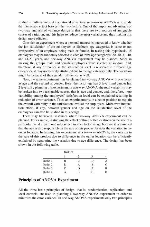
studied simultaneously. An additional advantage in two-way ANOVA is to study
the interaction effect between the two factors. One of the important advantages of
two-way analysis of variance design is that there are two sources of assignable
causes of variation, and this helps to reduce the error variance and thus making this
design more efficient.
Consider an experiment where a personal manger is interested to know whether
the job satisfaction of the employees in different age categories is same or not
irrespective of an employee being male or female. In testing this hypothesis, 15
employees may be randomly selected in each of three age categories: 20–30, 31–40,
and 41–50 years, and one-way ANOVA experiment may be planned. Since in
making the groups male and female employees were selected at random, and,
therefore, if any difference in the satisfaction level is observed in different age
categories, it may not be truly attributed due to the age category only. The variation
might be because of their gender difference as well.
Now, the same experiment may be planned in two-way ANOVA with one factor
as age and the second as gender. Here, the factor age has 3 levels and gender has
2 levels. By planning this experiment in two-way ANOVA, the total variability may
be broken into two assignable causes, that is, age and gender, and, therefore, more
variability among the employees’ satisfaction level can be explained resulting in
reduction of error variance. Thus, an experimenter is in a better position to explain
the overall variability in the satisfaction level of the employees. Moreover, interac-
tion effect, if any, between gender and age on the satisfaction level of the
employees can also be studied in this design.
There may be several instances where two-way ANOVA experiment can be
planned. For example, in studying the effect of three outlet locations on the sale of a
particular facial cream, one may select another factor as age because it is assumed
that the age is also responsible in the sale of this product besides the variation in the
outlet location. In framing this experiment as a two-way ANOVA, the variation in
the sale of this product due to difference in the outlet location can be efficiently
explained by separating the variation due to age difference. The design has been
shown in the following table.
District
1 2 3 4
Outlet 1 B C D A
Outlet 2 D A B C
Outlet 3 C D A B
Outlet 4 A B C D
Principles of ANOVA Experiment
All the three basic principles of design, that is, randomization, replication, and
local controls, are used in planning a two-way ANOVA experiment in order to
minimize the error variance. In one-way ANOVA experiments only two principles
256 8 Two-Way Analysis of Variance: Examining Influence of Two Factors. . .

i.e. randomization and replication are used to control the error variance whereas
in two-way ANOVA experiments all the three principles i.e. randomization, rep-
lication, and local control are used to control the error variance. The very purpose
of using these three principles of design is to enable the researcher to conclude with
more authority that the variation in the criterion variable is due to the identified
level of a particular factor.
In two-way ANOVA experiment, the principle of randomization means that the
samples in each group are selected in a random fashion so as to make the groups as
homogeneous as possible. The randomization avoids biases and brings control in
the experiment and helps in reducing the error variance up to a certain extent.
The principle of replication refers to studying the effect of two factors on more
than one subject in each cell. The logic is that one should get the same findings on
more than one subject. In two-way ANOVA experiment, the principle of replication
allows a researcher to study the significance of interaction between the two factors.
Interaction effect cannot be studied if there is only one observation in each cell.
The principle of local control refers to making the groups as homogeneous as
possible so that variation due to one or more assignable causes may be segregated
from the experimental error. Thus, the application of local control helps us in
reducing the error variation and making the design more efficient.
In the example discussed above, in studying the effect of age on job satisfaction
if the employees were divided only according to their age, then we would have
ignored the effect of gender on job satisfaction which would have increased
the experimental error. However, if the researcher feels that instead of gender
if the job satisfaction varies as per their salary structure, then the subjects may be
selected as per their salary bracket in different age categories. This might further
reduce the experimental error. Thus, maximum homogeneity can be ensured
among the observations in each cell by including the factor in the design which is
known to vary with the criterion variable.
Classification of ANOVA
By using the above-mentioned principles the two-way ANOVA can be used for
different designs. Some of the most popular designs where two-way ANOVA can
be used are discussed below.
Factorial Analysis of Variance
Two-way ANOVA is the most widely used in factorial designs. The factorial design
is used for more than one independent variable. The independent variables are also
referred to as factors. In factorial design, there are at least two or more factors.
Usually, two-way analysis of variance is used in factorial designs having two factors.
Classification of ANOVA 257

In this design, the effect of two factors (having different levels) is seen on the
dependent variable. Consider an experiment where age (A) and gender (B) are
taken as two factors whose effect has to be seen on the dependent variability,
sincerity. Further, let the factor A has three levels (20–30, 31–40, and 41–50 years)
and the factor B has two levels (Male and Female). Thus, in this design, 2 � 3, that
is, six combination of treatment groups need to be taken. This design facilitates
in studying the effect of both the factors A and B on the dependent variable. Further,
in this design, significance of the interaction effect between the two factors can
also be tested. The factorial design is very popular in the behavioral research, social
sciences, and humanities. This design has a few advantages over single-factor
designs. The most important aspect of the factorial design is that it can provide
some information about how factors interact or combine in the effect they have on the
dependent variable. The factorial design shall be discussed in detail while in solving
two-way ANOVA problem later in this chapter.
Repeated Measure Analysis of Variance
Another design where two-way ANOVA is used is the repeated measure design.
This design is also known as a within-subject design. In this design, same subject is
tested under repeated conditions over a time. The repeated measure design can be
considered to be an extension of the paired-samples t-test because in this case,
comparison is done between more than two repeated measures. The repeated
measure design is used to eliminate the individual differences as a source of
between-group differences. This helps to create a more powerful test. The only
care to be taken in the repeated measure design is that while testing the same subject
repeatedly, no carryover effect should be there.
Multivariate Analysis of Variance (MANOVA)
In this design, effect of two factors is studied on more than one dependent variable.
It is similar to the factorial design having two factors, but the only difference is that
here we have more than one dependent variable. At times, it makes sense to
combine the dependent variables for drawing the conclusion about the effects of
two factors on it. For instance, in an experiment, if the effect of teaching methods
and hostel facilities have to be seen on the overall academic performance
(consisting four subjects: Physics, Chemistry, Math, and English) of the students,
then it makes sense to see the effect of these two factors, that is, teaching methods
and hostel facilities on all the subjects together. Once the effect of any of these
factors is found to be significant, then the two-way ANOVA for each of the
dependent variable is applied.
258 8 Two-Way Analysis of Variance: Examining Influence of Two Factors. . .
In using two-way MANOVA, the dependent variables should neither be highly
correlated among themselves nor should they be totally uncorrelated. The benefit of
using MANOVA is that one can study the effect of each factor and their interaction
on the whole basket of dependent variables. It makes sense to study the effect of two
factors on the group of dependent variables like personality, employees, students,
etc. Personality is the sum total of many variables like honesty, sincerity, and
positivity; similarly, employees may be classified as male and female, whereas
students may be categories as undergraduate and postgraduate. At times, it may be
interesting to see the impact of two factors like age and education on the personality
of an individual. Once any of this factor’s effect on the personality as a whole is
significant, then the two-way analysis of variance may be applied for each of these
dimensions of the personality separately to see how these dimensions are affected
individually by the age and education.
Advantages of Two-Way ANOVA over One-Way ANOVA
Two-way ANOVA design is more efficient over one-way ANOVA because of the
following four reasons:
1. Unlike one-way ANOVA, the two-way ANOVA design facilitates us to test the
effect of two factors at the same time.
2. Since in two-way ANOVA variation is explained by two assignable causes, it
reduces the error variance. Due to this fact, two-way ANOVA design is more
efficient than one-way ANOVA.
3. In two-way ANOVA, one can test for independence of the factors provided there
is more than one observation per cell. However, number of observations in each
cell must be equal. On the other hand, in one-way ANOVA, one may have the
unequal number of scores in each group.
4. Besides reducing the error variance, two-way ANOVA also reduces the compu-
tation as it includes several one-way ANOVA.
Important Terminologies Used in Two-Way ANOVA
Factors
Independent variables are usually known as factors. In two-way ANOVA, the effectof two factors is studied on certain criterion variable. Each of the two factors may
have two or more levels. The degrees of freedom for each factor is equal to the
number of levels in the factor minus one.
Important Terminologies Used in Two-Way ANOVA 259

Treatment Groups
The number of treatments in two-way ANOVA experiment is equal to the number
of combinations of the levels of the two factors. For example, if the factor A has
2 levels, A1 and A2, and the factor B has 3 levels, B1, B2, and B3, then there will be
2 � 3 ¼ 6 different treatment groups A1B1, A1B2, A1B3, A2B1, A2B2, and A2B3.
Main Effect
The main effect is the effect of one independent variable (or factor) on the
dependent variable across all the levels of the other variable. The interaction is
ignored for this part. Just the rows or just the columns are used, not mixed. This is
the part which is similar to one-way analysis of variance. Each of the variances
calculated to analyze the main effects (rows and columns) is like between
variances. The degrees of freedom for the main effect are one less than its number
of levels. For example, if the factor A has r levels and factor B has c levels, then thedegrees of freedom for the factor A and B would be r � 1 and c � 1, respectively.
Interaction Effect
The joint effect of two factors on the dependent variable is known as interaction
effect. It can also be defined as the effect that one factor has on the other factor. The
degrees of freedom for the interaction is the product of degrees of freedom of both
the factors. If the factors A and B have levels r and c, respectively, then the degreesof freedom for the interaction would be (r � 1) � (c � 1).
Within-Group Variation
The within-group variation is the sum of squares within each treatment groups.
In two-way ANOVA, all treatment groups must have the same sample size. The
total number of treatment groups is the product of the number of levels for each
factor. The within variance is equal to within variation divided by its degrees of
freedom. The within group is also denoted as error. The within-group variation is
often denoted by SSE.
260 8 Two-Way Analysis of Variance: Examining Influence of Two Factors. . .

Two-Way ANOVA Model and Hypotheses Testing
Let us suppose that there are two factors A and B whose effects have to be tested on
the criterion variable X, and let the factors A and B have levels r and c, respectively,with n units per cell, then these scores can be written as follows:
Factor B
1 .. j .. c
1 X111 X1j1 X1c1
X112 .. X1j2 .. X1c2
. . .
X11n
T11
X1jn
T1j
X1cn
T1c
R1
Factor A i Xi11 Xij1 Xic1
Xi12 .. Xij2 .. Xic2
. . .
Xi1n
Ti1
Xijn
Tij
Xicn
Tic
Ri
r Xr11 Xrj1 Xrc1
Xr12 .. Xrj2 .. Xrc2
. . .
Xr1n
Tr1
Xrjn
Trj
Xrcn
Trc
Rr
C1 Cj Cc G ¼PRi ¼P
Cj
where
Xijk represents the kth score in the (i,j)th cell
Tij represents the total of all the n scores in the (i,j)th cell
G is the grand total of all the scores
Ri is the total of all the scores in ith level of the factor ACj is the total of all the scores in jth level of the factor BN is the total of all the scores and is equal to r � c � n
In two-way ANOVA, the total variability among the above-mentioned N scores
can be attributed to the variability due to row (or factor A), due to column (or factor
B), due to interaction (row � column (A � B)), and due to error. Thus, the total
variability can be broken into the following four components:
Total variability ¼ Variability due to Row SSRð Þ þ Variability due to Column SSCð Þþ Variability due to Interaction SSIð Þ þ Variability due to Error
or TSS ¼ SSRþ SSCþ SSIþ SSE (8.1)
Remark: SSE is the variability within group which was represented by SSw in one-
way ANOVA.
Two-Way ANOVA Model and Hypotheses Testing 261

The above-mentioned model is a two-way ANOVA model where it is assumed
that the variability among the scores may be due to row factor, column factor,
interaction due to row and column, and the error factor. Since the variation in the
group has been explained by the two factors instead of one factor in one-way
ANOVA, reduction of error variance is more in two-way ANOVA in comparison
to that of one-way ANOVA design. This makes this design more efficient than one-
way ANOVA. After developing the above-mentioned model of variability, it is
required to test whether the effects of these factors are significant or not in
explaining the variation in the data. The significance of these components is tested
by means of using F-test.
(a) Hypotheses construction: The hypotheses which are being tested in two-way
ANOVA are as follows:
(i) H0 : mA1¼ mA2
¼ . . . ¼ mAr
(The population means of all the levels of the factor A are equal. This is like
the one-way ANOVA for the row factor.)
(ii) H0 : mB1¼ mB2
¼ . . . ¼ mBc
(The population means of all the levels of the factor B are equal. This is like
the one-way ANOVA for the column factor.)
(iii) H0: There is no interaction between factors A and B.(This is similar to performing a test for independence with contingency
table.)
The above-mentioned null hypotheses are tested against the alternative
hypothesis that at least one mean is different.
If the null hypotheses mentioned in (i) and (ii) are rejected, then it is
concluded that the variability due to factor is significant, and it is inferred
that the means of all the groups in that factor is not same. On the other hand, if
the null hypothesis is failed to be rejected, one may draw the inference that all
group means are equal. If the hypothesis mentioned in (iii) is rejected, then one
may conclude that there is a significant interaction between the factors A and B.In other words, it may be concluded that the pattern of differences of group
means in factor A is not the same in different levels of factor B. This fact shallbe discussed in detail while solving the Example 8.1. Thus, if the effects of
factors A and B having levels m and n, respectively, are to be seen on the
criterion variable, then the following steps will explain the procedure of testing
the hypotheses:
(b) Level of significance: The level of significance may be chosen beforehand.
Usually, it is taken as .05 or .01.
(c) Statistical test: The F-test is used to compare the variability between levels of a
factor with that of variability within groups. If F-value is significant, it indicatesthat variability between levels of the factor groups is significantly higher than
the variability within groups; in that case, the null hypothesis of no difference
between the group means is rejected. Before computing F-value, it is requiredto compute the total sum of squares (TSS), sum of squares due to row factor
262 8 Two-Way Analysis of Variance: Examining Influence of Two Factors. . .

A (SSR), sum of squares due to column factor B (SSC), sum of squares due to
interaction A � B (SSI), and sum of squares due to error (SSE).
(i) Total sum of squares (TSS): It represents the total variation present in the
data set and is usually represented by TSS. It is defined as the sum of the
squared deviations of all the scores in the data set from their grand mean.
The TSS is computed by the following formula:
TSS ¼Xri¼1
Xcj¼1
Xnk¼1
Xijk � G
N
� �2
after solving
¼Xi
Xj
Xk
X2ijk �
G2
N(8.2)
Since the degrees of freedom for the TSS are N � 1, therefore mean sum
of squares is computed by dividing the TSS by N � 1.
(ii) Sum of squares due to row factor (SSR): It is the measure of variation
between the row group means and is usually denoted by SSR. This is also
known as the variation due to row factor (one of the assignable causes).
The sum of squares due to row is computed as follows:
SSR ¼Xri¼1
R2i
nc� G2
N(8.3)
Since r levels of row factor A is compared in two-way ANOVA, the
degrees of freedom for SSR are given by r � 1. Thus, mean sum of squares
for row factor is obtained by dividing the SSR by its degrees of freedom
r � 1.
(iii) Sum of squares due to column factor (SSC): It is the measure of variation
between the column group means and is usually denoted by SSC. This
explains the variation due to column factor (one of the assignable causes).
The sum of squares due to column factor is computed as
SSC ¼Xcj¼1
C2j
nr� G2
N(8.4)
The degrees of freedom for SSC are given by c � 1 as there are c column
group means that are required to be compared. The mean sum of square for
column factor is obtained by dividing SSC by c � 1.
Two-Way ANOVA Model and Hypotheses Testing 263
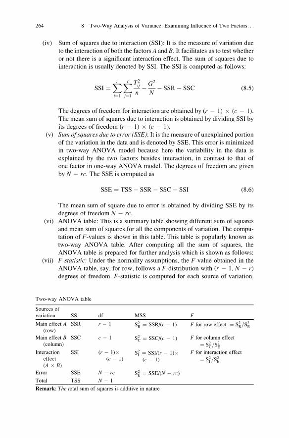
(iv) Sum of squares due to interaction (SSI): It is the measure of variation due
to the interaction of both the factors A and B. It facilitates us to test whetheror not there is a significant interaction effect. The sum of squares due to
interaction is usually denoted by SSI. The SSI is computed as follows:
SSI ¼Xri¼1
Xcj¼1
T2ij
n� G2
N� SSR� SSC (8.5)
The degrees of freedom for interaction are obtained by (r � 1) � (c � 1).
The mean sum of squares due to interaction is obtained by dividing SSI by
its degrees of freedom (r � 1) � (c � 1).
(v) Sum of squares due to error (SSE): It is the measure of unexplained portion
of the variation in the data and is denoted by SSE. This error is minimized
in two-way ANOVA model because here the variability in the data is
explained by the two factors besides interaction, in contrast to that of
one factor in one-way ANOVA model. The degrees of freedom are given
by N � rc. The SSE is computed as
SSE ¼ TSS� SSR� SSC� SSI (8.6)
The mean sum of square due to error is obtained by dividing SSE by its
degrees of freedom N � rc.(vi) ANOVA table: This is a summary table showing different sum of squares
and mean sum of squares for all the components of variation. The compu-
tation of F-values is shown in this table. This table is popularly known as
two-way ANOVA table. After computing all the sum of squares, the
ANOVA table is prepared for further analysis which is shown as follows:
(vii) F-statistic: Under the normality assumptions, the F-value obtained in the
ANOVA table, say, for row, follows a F-distribution with (r � 1, N � r)degrees of freedom. F-statistic is computed for each source of variation.
Two-way ANOVA table
Sources of
variation SS df MSS F
Main effect A(row)
SSR r � 1 S2R ¼ SSR/(r � 1) F for row effect ¼ S2R=S2E
Main effect B(column)
SSC c � 1 S2C ¼ SSC/(c � 1) F for column effect
¼ S2C=S2E
Interaction
effect
(A � B)
SSI (r � 1)�(c � 1)
S2I ¼ SSI/(r � 1)�(c � 1)
F for interaction effect
¼ S2I =S2E
Error SSE N � rc S2E ¼ SSE/(N � rc)
Total TSS N � 1
Remark: The total sum of squares is additive in nature
264 8 Two-Way Analysis of Variance: Examining Influence of Two Factors. . .

This test statistic F is used to test the null hypothesis of no difference
among the group means.
(d) Decision criteria: The tabulated value of F at .05 or .01 level of significance
with different degrees of freedom may be obtained from Tables A.4 or A.5,
respectively in the Appendix. If the calculated value of F is greater than the
tabulated F, the null hypothesis is rejected, and in that case, at least one of the
means is different than others. Since ANOVA does not tell us where the
difference lies, post hoc test is used to get the clear picture. There are several
post hoc tests which can be used but least significant difference (LSD) test is
generally used in equal sample sizes. However, one may use other post hoc tests
like Scheffe’s, Tukey, Bonferroni, or Duncan as well.
In all the post hoc tests, a critical difference is computed at a particular level
of significance, and if the difference of any pair of observed means is higher
than the critical difference, it is inferred that the mean difference is significant
otherwise insignificant. By comparing all pair of group means, conclusion is
drawn as to which group mean is the highest. The detail procedure of applying
the post hoc test has been discussed in the solved Example 8.1.
In LSD test, the critical difference (CD) is computed as
CD ¼ t:05 N � rcð Þ �ffiffiffiffiffiffiffiffiffiffiffiffiffiffiffi2MSSE
n
r(8.7)
where the symbols have their usual meanings.
This critical difference (CD) is used for comparing differences in all the pair
of means.
The SPSS output provides the significance value (p-value) for each of the F-statistics computed in two-way ANOVA table. If p-value is less than .05, Fwould be significant. Post hoc test for comparing means is applied for those
factors and interaction whose F-value is significant. The SPSS also provides p-values (significant value) for each pair of means in row, column, and interaction
to test the significance of difference between them. If p-value for any pair of
means is less than .05, it is concluded that means are significantly different
otherwise not.
Assumptions in Two-Way Analysis of Variance
Following assumptions need to be satisfied while using the two-way ANOVA
design:
(a) The population from which the samples are drawn must be normally
distributed.
(b) The samples must be independent.
(c) The population variances must be equal.
(d) The sample size must be same in each cell.
Two-Way ANOVA Model and Hypotheses Testing 265

Situation Where Two-Way ANOVA Can Be Used
In two-way ANOVA, we investigate the effect of main effects along with the
interaction effect of two factors on dependent variable. The following situation
shall develop an insight among the researchers to appreciate the use of this analysis.
Consider a situation where a mobile company is interested to examine the effect
of gender and age of the customers on the frequency of short messaging service
(sms) sent per week. Each person may be classified according to gender (men and
women) and age category (16–25, 26–35, and 36–45 years). Thus, there will be six
groups, one for each combination of gender and age. Random sample of equal size
in each group may be drawn, and each person may be asked about the number of
sms he or she sends per week. In this situation, there are three main research
questions that can be answered:
(a) Whether the number of sms sent depends on gender
(b) Whether the number of sms sent depends on age
(c) Whether the number of sms sent depends on gender differently for different age
categories of age, and vice versa
All these questions can be answered through testing of hypothesis in two-way
ANOVA model. The first two questions simply ask whether sending sms depends
on age and gender. On the other hand, the third question asks whether sending sms
depends on gender differently for people in different age category, or whether
sending sms depends on age differently for men and women. This is because one
may think that men send more sms than women in 18–25 years age category, but
women send more sms than men in 26–55 years age category. After applying the
two-way ANOVAmodel, one may be able to explain the above-mentioned research
questions in the following manner:
whether the factor gender has a significant impact on the number of sms sent
irrespective of their age categories. And if it is so, one may come to know whether
men send more sms than women or vice versa, irrespective of their age categories.
Similarly, one can test whether the factor age has a significant impact on the
number of sms sent irrespective of gender. And if age factor is significant, one can
know that in which age category people send more sms irrespective of their gender.
The most important aspect of two-way ANOVA is to know the presence of
interaction effect of gender and age on sending the sms. One may test whether these
two factors, that is, gender and age, are independent to each other in deciding the
number of sms sent. The interaction analysis allows us to compare the average sms
sent in different age categories in each of the men and women groups separately.
Similarly, it also provides the comparison of the average sms sent by the men and
women in different age categories separately.
The information provided through this analysis may be used by the marketing
department to chalk out their promotional strategy for men and women separately
in different age categories for the mobile users.
266 8 Two-Way Analysis of Variance: Examining Influence of Two Factors. . .
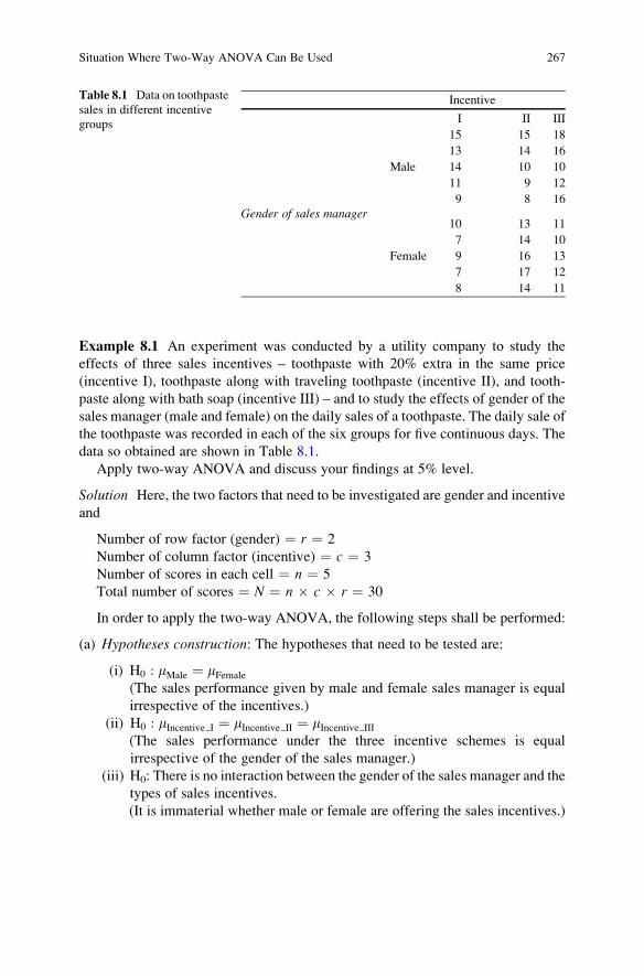
Example 8.1 An experiment was conducted by a utility company to study the
effects of three sales incentives – toothpaste with 20% extra in the same price
(incentive I), toothpaste along with traveling toothpaste (incentive II), and tooth-
paste along with bath soap (incentive III) – and to study the effects of gender of the
sales manager (male and female) on the daily sales of a toothpaste. The daily sale of
the toothpaste was recorded in each of the six groups for five continuous days. The
data so obtained are shown in Table 8.1.
Apply two-way ANOVA and discuss your findings at 5% level.
Solution Here, the two factors that need to be investigated are gender and incentive
and
Number of row factor (gender) ¼ r ¼ 2
Number of column factor (incentive) ¼ c ¼ 3
Number of scores in each cell ¼ n ¼ 5
Total number of scores ¼ N ¼ n � c � r ¼ 30
In order to apply the two-way ANOVA, the following steps shall be performed:
(a) Hypotheses construction: The hypotheses that need to be tested are:
(i) H0 : mMale ¼ mFemale
(The sales performance given by male and female sales manager is equal
irrespective of the incentives.)
(ii) H0 : mIncentive I ¼ mIncentive II ¼ mIncentive III
(The sales performance under the three incentive schemes is equal
irrespective of the gender of the sales manager.)
(iii) H0: There is no interaction between the gender of the sales manager and the
types of sales incentives.
(It is immaterial whether male or female are offering the sales incentives.)
Table 8.1 Data on toothpaste
sales in different incentive
groups
Incentive
I II III
15 15 18
13 14 16
Male 14 10 10
11 9 12
9 8 16
10 13 11Gender of sales manager
7 14 10
Female 9 16 13
7 17 12
8 14 11
Situation Where Two-Way ANOVA Can Be Used 267
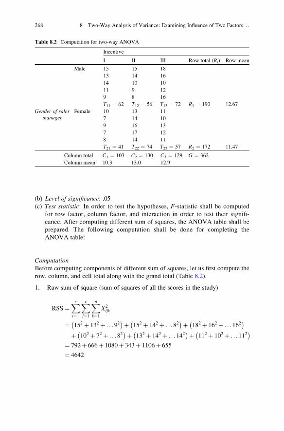
(b) Level of significance: .05(c) Test statistic: In order to test the hypotheses, F-statistic shall be computed
for row factor, column factor, and interaction in order to test their signifi-
cance. After computing different sum of squares, the ANOVA table shall be
prepared. The following computation shall be done for completing the
ANOVA table:
ComputationBefore computing components of different sum of squares, let us first compute the
row, column, and cell total along with the grand total (Table 8.2).
1. Raw sum of square (sum of squares of all the scores in the study)
RSS¼Xri¼1
Xcj¼1
Xnk¼1
X2ijk
¼ 152 þ 132 þ . . .92� �þ 152 þ 142 þ . . .82
� �þ 182 þ 162 þ . . .162� �
þ 102 þ 72 þ . . .82� �þ 132 þ 142 þ . . .142
� �þ 112 þ 102 þ . . .112� �
¼ 792þ 666þ 1080þ 343þ 1106þ 655
¼ 4642
Table 8.2 Computation for two-way ANOVA
Incentive
I II III Row total (Ri) Row mean
Male 15 15 18
13 14 16
14 10 10
11 9 12
9 8 16
T11 ¼ 62 T12 ¼ 56 T13 ¼ 72 R1 ¼ 190 12.67
Gender of salesmanager
Female 10 13 11
7 14 10
9 16 13
7 17 12
8 14 11
T21 ¼ 41 T22 ¼ 74 T23 ¼ 57 R2 ¼ 172 11.47
Column total C1 ¼ 103 C2 ¼ 130 C3 ¼ 129 G ¼ 362
Column mean 10.3 13.0 12.9
268 8 Two-Way Analysis of Variance: Examining Influence of Two Factors. . .

2. Correction factor ¼ CF
¼ G2
N¼ 3622
30¼ 4368:13
3. Total sum of squares ¼ TSS
¼Xi
Xj
Xk
X2ijk �
G2
N¼ RSS� CF
¼ 4642� 4368:13 ¼ 273:87
4. Sum of squares due to row factor genderð Þ ¼ SSR
¼Xri¼1
R2i
nc� G2
N¼ 1902 þ 1722
5� 3� 4368:13
¼ 10:80
5. Sum of squares due to column factor incentivesð Þ ¼ SSC
¼Xcj¼1
C2j
nr� G2
N
¼ 1032 þ 1302 þ 1292
5� 2
� 4368:13 ¼ 46:87
6. Sum of squares due to interaction ¼ SSI
¼Xri¼1
Xcj¼1
T2ij
n� G2
N� SSR� SSC
¼ 622 þ 562 þ 722 þ 412 þ 742 þ 572
5
� 4368:13� 10:80� 46:87
¼ 4514� 4425:8 ¼ 88:20
7. Sum of squares due to error ¼ SSE
¼TSS� SSR� SSC� SSI
¼ 273:87� 10:80� 46:87� 88:20
¼ 128
Tabulated value of F can be seen from Table A.4 in the Appendix. Thus, from
Table A.4, the value of F.05 (1,24) ¼ 4.26 and F.05 (2,24) ¼ 3.40.
In Table 8.3, since the calculated value of F for incentives and interaction is
greater than their corresponding tabulated value of F, these two F-ratios are
significant. However, F-value for gender is not significant.
Situation Where Two-Way ANOVA Can Be Used 269

Post hoc test shall be used to further analyze the column factor (incentives) and
the interaction effect.
Post Hoc Test for Column Factor (Incentives)LSD test shall be used to find the critical difference for comparing the means of
the groups in the column factor. The critical difference (CD) is given by
CD at :05 significance level ¼ t:05 24ð Þ �ffiffiffiffiffiffiffiffiffiffiffiffiffiffiffi2MSSE
n� r
r
¼ 2:064�ffiffiffiffiffiffiffiffiffiffiffiffiffiffiffiffiffi2� 5:33
5� 2
r½From Table A:2 in the Appendix; t:05ð24Þ ¼ 2:064�
¼ 2:064� 1:03
¼ 2:13
Table 8.4 shows that the mean difference between II and III incentive groups is
less than the critical difference (¼2.13); hence, there is no difference between these
two incentive groups. To show this, a line has been drawn below these two group
means. On the other hand, there is a significant difference between the means of II
and I as well as III and I incentive groups. Thus, it may be concluded that the II and
III incentives are equally effective and better than Ist incentive in enhancing the
sale of the toothpaste irrespective of the gender of the sales manager.
Table 8.4 Mean sale in
different incentive groups
(both gender combined)
Incentives CD at 5% level
II III I
13.0 12.9 10.3 1.48
“ ” Denotes no difference between the means
at .05 level
Table 8.3 Two-way ANOVA table for the data on sales of toothpaste
Source of variation
Sum of
squares (SS) df
Mean sum of
squares (MSS) FTab. F at
5% level
Gender 10.80 r � 1 ¼ 1 10.80 2.03 4.26
Incentives 46.87 c � 1 ¼ 2 23.44 4.398* 3.40
Interaction (gender*
incentives)
88.20 (r � 1) �(c � 1) ¼ 2
44.10 8.27* 3.40
Error 128.00 N � rc ¼ 24 5.33
Corrected total 273.87 N � 1 ¼ 29
*Significant at 5% level
270 8 Two-Way Analysis of Variance: Examining Influence of Two Factors. . .

Post Hoc Test for Interaction (Gender � Incentives)Since interaction effect is significant, comparison shall be made among the means
of each incentive groups in each gender. Similarly, mean comparison shall also be
made between male and female groups in each of the incentive groups. Since the
cell size is similar, the critical difference for row comparison in each column and
for column comparison in each row shall be same. The CD using LSD test shall be
obtained by
CD at :05 significance level ¼ t:05 24ð Þ �ffiffiffiffiffiffiffiffiffiffiffiffiffiffiffi2MSSE
n
r
¼ 2:064�ffiffiffiffiffiffiffiffiffiffiffiffiffiffiffiffiffi2� 5:33
5
r¼ 2:064� 1:46
¼ 3:01
Table 8.5 provides the post hoc comparison of means of male and female groups
in each of the three incentive groups. Since the mean difference between male and
female in each of the three incentive groups is higher than the critical difference,
these differences are significant at 5% level. Further, it may be concluded that the
average sales of male group in I and III incentives groups are higher than that of
female group whereas average sales of female is higher than that of male in II
incentive group.
Table 8.6 shows the comparison of different incentive groups in each of the gender
group. It can be seen from this table that in male section, average sales are signifi-
cantly different in III and II incentive groups, whereas average sales in the III and I
incentive groups as well as I and II incentive groups are same. On the other hand, in
female section, the average sales in all the three incentive groups are significantly
different from each other.
Table 8.5 Comparison
of mean sale of toothpaste
between male and female
groups in each of the three
incentive groups
Gender
Incentives Male Female Mean diff. CD at 5% level
I 12.4 8.2 4.2* 2.10
II 11.2 14.8 3.6* 2.10
III 14.4 11.4 3.0* 2.10
*Significant at 5% level
Table 8.6 Comparison of mean sale of toothpaste among different
incentive groups in each of the two gender groups
Gender Incentives CD at 5% level
Male 14.4 (III) 12.4 (I) 11.2 (II) 2.10
Female 14.8 (II) 11.4 (III) 8.2 (I) 2.10
Remark: Arrange means of the groups in descending order
Situation Where Two-Way ANOVA Can Be Used 271

Thus, on the basis of the given data, the result suggests that IIIrd incentive
should be preferred if it is promoted by the male sales manager whereas the sales of
the toothpaste would increase if it is promoted by the female sales manager using
IInd incentive.
Solved Example of Two-Way ANOVA Using SPSS
Example 8.2 A chocolate manufacturing company wanted to know the impact of
color and sweetness of its chocolates on buying decision of the customers. Data in
Table 8.7 shows the number of units sold per day in a city for five consecutive days.
Apply two-way analysis of variance to see whether the factors sweetness and color
have significant effect on the sale of chocolates. Also test the significance of
interaction between these two factors and discuss your findings at 5% level.
Solution Here, two main factors, namely, sweetness and color as well as interac-
tion between sweetness and color, need to be investigated. Thus, following three
hypotheses shall be tested:
(i) H0 : mSemi Sweet ¼ mBitter Sweet ¼ mUn Sweet
(The sales of semisweet, bittersweet, and unsweetened chocolates are same
irrespective of the color of the chocolate.)
(ii) H0 : mWhite ¼ mMilk ¼ mDark(The sales of white, milk, and dark chocolates are same irrespective of the
sweetness of the chocolate.)
(iii) H0: There is no interaction between the sweetness and color of the chocolate.
Table 8.7 Data on sale
of chocolates of different
flavours and colours
Chocolate color
Sweetness White Milk Dark
Semisweet chocolate 25 20 35
20 15 32
22 17 31
28 21 42
23 25 30
Bittersweet chocolate 28 32 15
24 35 22
32 37 25
32 38 12
23 29 20
Unsweetened chocolate 26 20 15
24 15 12
32 17 10
26 21 22
31 25 13
272 8 Two-Way Analysis of Variance: Examining Influence of Two Factors. . .

(It is immaterial whether any color of the chocolates is semisweet, bittersweet,
or unsweetened.)
The SPSS output for two-way analysis of variance provides F-values for the
sweetness factor, color factor, and interaction (sweetness � color) along with
their significant values (p-values). The F-values for these factors and interaction
shall be significant if their p-values are less than .05. For any factor or interaction ifthe F-value is significant, then a post hoc test shall be applied to compare the paired
means. SPSS provides option to choose any of the post hoc tests for comparing the
significance of mean difference.
In this example, since the sample sizes are equal, LSD test shall be used as a post
hoc test for comparing group means. The SPSS output provides the significance
values (p-values) for the difference of each pair of group means. The significance of
difference between pair of group means is tested by using these p-values rather thancomputing the critical differences as is done in case of solving two-way ANOVA
manually.
Computation in Two-Way ANOVA Using SPSS
(a) Preparing data file
(i) Starting the SPSS: Use the below-mentioned command sequence to start
SPSS on your system:
Start ! Programs ! IBM SPSS Statistics ! IBM SPSS Statistics 20
After clicking the Type in Data, you will be taken to the Variable View
option for defining the variables in the study.
(ii) Defining variables: There are three variables in this example, namely, sales,
sweetness, and color. Since sales were measured on ratio scale, it has been
defined as a scale variable, whereas sweetness and color were measured on
nominal scale hence they have been defined as nominal variables. The
procedure of defining the variables and their characteristics in SPSS is as
follows:
1. Click Variable View to define variables and their properties.
2. Write short name of the variables as Sale, Sweetness, and Colour underthe column heading Name.
3. Under the column heading Label, define full name of these variables as
Chocolate_Sale, Chocolate_Sweetness, and Chocolate_Colour. Alter-nate names may also be chosen for describing these variables.
4. Under the column heading Measure, select the option “Scale” for the
variable Sale and “Nominal” for the variables Sweetness and Colour.
Solved Example of Two-Way ANOVA Using SPSS 273
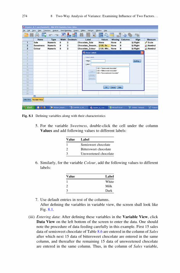
5. For the variable Sweetness, double-click the cell under the column
Values and add following values to different labels:
Value Label
1 Semisweet chocolate
2 Bittersweet chocolate
3 Unsweetened chocolate
6. Similarly, for the variable Colour, add the following values to different
labels:
Value Label
1 White
2 Milk
3 Dark
7. Use default entries in rest of the columns.
After defining the variables in variable view, the screen shall look like
Fig. 8.1.
(iii) Entering data: After defining these variables in the Variable View, click
Data View on the left bottom of the screen to enter the data. One should
note the procedure of data feeding carefully in this example. First 15 sales
data of semisweet chocolate of Table 8.6 are entered in the column of Salesafter which next 15 data of bittersweet chocolate are entered in the same
column, and thereafter the remaining 15 data of unsweetened chocolate
are entered in the same column. Thus, in the column of Sales variable,
Fig. 8.1 Defining variables along with their characteristics
274 8 Two-Way Analysis of Variance: Examining Influence of Two Factors. . .
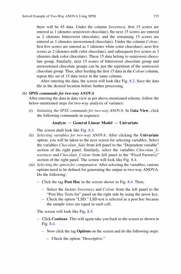
there will be 45 data. Under the column Sweetness, first 15 scores are
entered as 1 (denotes semisweet chocolate), the next 15 scores are entered
as 2 (denotes bittersweet chocolate), and the remaining 15 scores are
entered as 3 (denotes unsweetened chocolate). Under the column Colour,first five scores are entered as 1 (denotes white color chocolate), next five
scores as 2 (denotes milk color chocolate), and subsequent five scores as 3
(denotes dark color chocolate). These 15 data belong to semisweet choco-
late group. Similarly, next 15 scores of bittersweet chocolate group and
unsweetened chocolate groups can be just the repetition of the semisweet
chocolate group. Thus, after feeding the first 15 data in the Colour column,
repeat this set of 15 data twice in the same column.
After entering the data, the screen will look like Fig. 8.2. Save the data
file in the desired location before further processing.
(b) SPSS commands for two-way ANOVAAfter entering the data in data view as per above-mentioned scheme, follow the
below-mentioned steps for two-way analysis of variance:
(i) Initiating the SPSS commands for two-way ANOVA: In Data View, click
the following commands in sequence:
Analyze ! General Linear Model ! Univariate
The screen shall look like Fig. 8.3.
(ii) Selecting variables for two-way ANOVA: After clicking the Univariate
option, you will be taken to the next screen for selecting variables. Select
the variables Chocolate_Sale from left panel to the “Dependent variable”
section of the right panel. Similarly, select the variables Chocolate_S-weetness and Chocolate_Colour from left panel to the “Fixed Factor(s)”
section of the right panel. The screen will look like Fig. 8.4.
(iii) Selecting the option for computation: After selecting the variables, variousoptions need to be defined for generating the output in two-way ANOVA.
Do the following:
– Click the tag Post Hoc in the screen shown in Fig. 8.4. Then,
– Select the factors Sweetness and Colour from the left panel to the
“Post Hoc Tests for” panel on the right side by using the arrow key.
– Check the option “LSD.” LSD test is selected as a post hoc because
the sample sizes are equal in each cell.
The screen will look like Fig. 8.5.
– Click Continue. This will again take you back to the screen as shown inFig. 8.4.
– Now click the tag Options on the screen and do the following steps:
– Check the option “Descriptive.”
Solved Example of Two-Way ANOVA Using SPSS 275
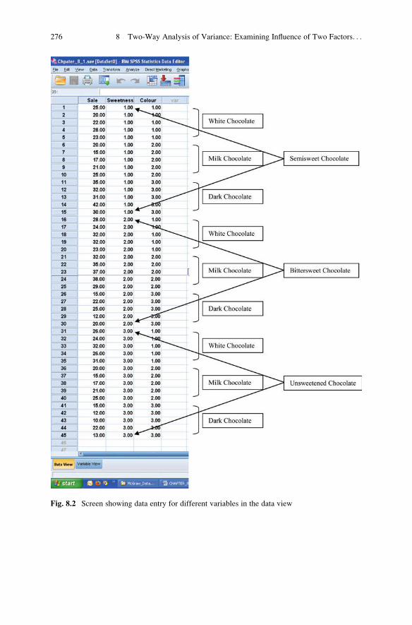
Fig. 8.2 Screen showing data entry for different variables in the data view
276 8 Two-Way Analysis of Variance: Examining Influence of Two Factors. . .

Fig. 8.3 Screen showing SPSS commands for two-way ANOVA
Fig. 8.4 Screen showing selection of variables for two-way ANOVA
Solved Example of Two-Way ANOVA Using SPSS 277

– Select the variables OVERALL, Sweetness, Colour, and Sweet-ness � Colour from the left panel and bring them into the “Dis-
play Means for” section of the right panel.
– Check the option “Compare main effects.”
– Ensure the value of Significance level as .05 in the box. The
screen for these options shall look like as shown in Fig. 8.6.
– Click Continue to go back to the main screen.
After selecting the options, the screen shown in Fig. 8.4 shall be
restored.
– Press OK.
(c) Getting the outputAfter clicking OK in the screen shown in Fig. 8.4, various outputs shall be
generated in the output window. Relevant outputs may be selected by using
Fig. 8.5 Screen showing options for post hoc test
278 8 Two-Way Analysis of Variance: Examining Influence of Two Factors. . .

right click of the mouse and may be copied in the word file. Here, the following
outputs shall be selected:
1. Descriptive statistics
2. Two-way ANOVA table
3. Pairwise comparisons of sweetness groups (all color groups combined)
4. Pairwise comparisons of different color groups (all sweetness groups
combined)
In this example, all the identified outputs so generated by the SPSS will look
like as shown in Tables 8.8, 8.9, 8.10, and 8.11.
In order to interpret the findings, these outputs may be rearranged so that it can
directly be used in your project. These rearranged formatted tables have been
shown under the heading “Model Way of Writing the Results” in the next
section.
Model Way of Writing the Results of Two-Way ANOVAand Its Interpretations
The outputs so generated in the SPSS may be presented in user-friendly format by
selecting the relevant details from Tables 8.8, 8.9, 8.10, and 8.11 and making some
slight modifications. Further, if the interaction is significant, it is not possible to
compare the cell means by using the outputs of SPSS. However, critical difference
can be computed by using these outputs for testing the significance of mean
Fig. 8.6 Screen showing options for descriptive statistics and comparison of main effects
Solved Example of Two-Way ANOVA Using SPSS 279

difference among different groups. The procedure of comparing group means has
been discussed later in this section.
The first important table consisting F-values for the factors and interaction can
be reproduced by deleting some of the contents of Table 8.9. The information so
reduced is shown in Table 8.12.
The p-values for the Sweetness, Color, and Interaction (Sweetness � Color) in
Table 8.12 are less than .05; hence, all the three F-values are significant at 5% level.
Thus, the null hypothesis for the Sweetness factor, Color factor, and Interaction
(Sweetness � Color) may be rejected at .05 level of significance. Now the post hoc
comparison analysis shall be done for these factors and interaction. These analyses
are shown below.
Table 8.8 Descriptive
statisticsSweetness Color Mean Std. dev. N
Semisweet chocolate White 23.60 3.04959 5
Milk 19.60 3.84708 5
Dark 34.00 4.84768 5
Total 25.73 7.28469 15
Bittersweet chocolate White 27.80 4.26615 5
Milk 34.20 3.70135 5
Dark 18.80 5.26308 5
Total 26.93 7.73181 15
Unsweetened chocolate White 27.80 3.49285 5
Milk 19.60 3.84708 5
Dark 14.40 4.61519 5
Total 20.60 6.81175 15
Total White 26.40 3.94244 15
Milk 24.47 7.94505 15
Dark 22.40 9.81107 15
Total 24.42 7.64106 45
Dependent variable: Chocolate_Sale
Table 8.9 Two-way ANOVA table generated by the SPSS
Source Type III sum df Mean square of squares F Sig.
Corrected model 1946.978a 8 243.372 14.086 .000
Intercept 26840.022 1 26840.022 1553.44 .000
Sweetness 339.511 2 169.756 9.825 .000
Color 120.044 2 60.022 3.474 .042
Sweetness * color 1487.422 4 371.856 21.522 .000
Error 622.000 36 17.278
Total 29409.000 45
Corrected total 2568.977 44
Dependent variable: Chocolate_SaleaR squared ¼ .758 (adjusted R squared ¼ .704)
280 8 Two-Way Analysis of Variance: Examining Influence of Two Factors. . .

Table 8.10 Pairwise comparison of different sweetness groups
95% Confidence
interval for
differencea
(I)Chocolate_Sweetness
(J)Chocolate_Sweetness
Mean diff.
(I – J)Std.
error
Sig.a
(p-value)Lower
bound
Upper
bound
Semisweet chocolate Bittersweet chocolate �1.200 1.518 .434 �4.278 1.878
Unsweetened
chocolate
5.133* 1.518 .002 2.055 8.212
Bittersweet chocolate Semisweet chocolate 1.200 1.518 .434 �1.878 4.278
Unsweetened
chocolate
6.333* 1.518 .000 3.255 9.412
Unsweetened
chocolate
Semisweet chocolate �5.133* 1.518 .002 �8.212 �2.055
Bittersweet chocolate �6.333* 1.518 .000 �9.412 �3.255
Dependent variable: Chocolate_Sale
Based on estimated marginal means
*The mean difference is significant at the .05 levelaAdjustment for multiple comparisons: least significant difference (equivalent to no adjustments)
Table 8.11 Pairwise comparison of different color groups
95% Confidence
interval for differencea
(I)Chocolate_Colour
(J)Chocolate_Colour
Mean diff.
(I – J)Std.
error Sig.aLower
bound
Upper
bound
White Milk 1.933 1.518 .211 �1.145 5.012
Dark 4.000* 1.518 .012 .922 7.078
Milk White �1.933 1.518 .211 �5.012 1.145
Dark 2.067 1.518 .182 �1.012 5.145
Dark White �4.000* 1.518 .012 �7.078 -.922
Milk �2.067 1.518 .182 �5.145 1.012
Dependent variable: Chocolate_Sale
Based on estimated marginal means
*The mean difference is significant at the .05 levelaAdjustment for multiple comparisons: least significant difference (equivalent to no adjustments)
Table 8.12 Two-way ANOVA table for the data on chocolate sale
Source of variation
Sum of squares
(SS) df
Mean sum of
squares (MSS) F p-value (sig.)
Sweetness 339.51 2 169.76 9.83 .000
Color 120.04 2 60.02 3.47 .042
Sweetness � color 1,487.42 4 371.86 21.52 .000
Error 622.00 36 17.28
Corrected total 2,568.977 44
Solved Example of Two-Way ANOVA Using SPSS 281
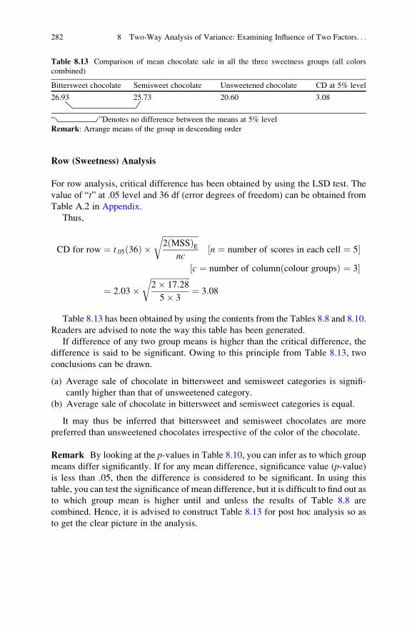
Row (Sweetness) Analysis
For row analysis, critical difference has been obtained by using the LSD test. The
value of “t” at .05 level and 36 df (error degrees of freedom) can be obtained from
Table A.2 in Appendix.
Thus,
CD for row ¼ t:05 36ð Þ �ffiffiffiffiffiffiffiffiffiffiffiffiffiffiffiffiffiffi2 MSSð ÞE
nc
rn ¼ number of scores in each cell ¼ 5½ �
½c ¼ number of column colour groupsð Þ ¼ 3�
¼ 2:03�ffiffiffiffiffiffiffiffiffiffiffiffiffiffiffiffiffiffiffiffi2� 17:28
5� 3
r¼ 3:08
Table 8.13 has been obtained by using the contents from the Tables 8.8 and 8.10.
Readers are advised to note the way this table has been generated.
If difference of any two group means is higher than the critical difference, the
difference is said to be significant. Owing to this principle from Table 8.13, two
conclusions can be drawn.
(a) Average sale of chocolate in bittersweet and semisweet categories is signifi-
cantly higher than that of unsweetened category.
(b) Average sale of chocolate in bittersweet and semisweet categories is equal.
It may thus be inferred that bittersweet and semisweet chocolates are more
preferred than unsweetened chocolates irrespective of the color of the chocolate.
Remark By looking at the p-values in Table 8.10, you can infer as to which groupmeans differ significantly. If for any mean difference, significance value (p-value)is less than .05, then the difference is considered to be significant. In using this
table, you can test the significance of mean difference, but it is difficult to find out as
to which group mean is higher until and unless the results of Table 8.8 are
combined. Hence, it is advised to construct Table 8.13 for post hoc analysis so as
to get the clear picture in the analysis.
Table 8.13 Comparison of mean chocolate sale in all the three sweetness groups (all colors
combined)
Bittersweet chocolate Semisweet chocolate Unsweetened chocolate CD at 5% level
26.93 25.73 20.60 3.08
“ ”Denotes no difference between the means at 5% level
Remark: Arrange means of the group in descending order
282 8 Two-Way Analysis of Variance: Examining Influence of Two Factors. . .

Column (Color) Analysis
For column analysis, critical difference has been obtained by using the LSD test as
there are equal numbers of samples in each column.
Thus,
CD for column ¼ t:05 36ð Þ �ffiffiffiffiffiffiffiffiffiffiffiffiffiffiffiffiffiffi2 MSSð ÞE
nr
rn ¼ number of scores in each cell ¼ 5½ �
½r ¼ number of row sweetness groupsð Þ ¼ 3�
¼ 2:03�ffiffiffiffiffiffiffiffiffiffiffiffiffiffiffiffiffiffiffiffi2� 17:28
5� 3
r¼ 3:08
Table 8.14 has been obtained from the contents in Tables 8.8 and 8.11.
From Table 8.14, the following two conclusions can be drawn:
(a) There is no difference in the average sale of white and milk chocolate. Similarly
average sale of milk and dark chocolate is also same.
(b) Average sale of white chocolates is significantly higher than that of dark
chocolates.
Thus, it may be inferred, in general, that the mean sale of the white chocolates is
more in comparison to that of dark chocolate irrespective of the type of sweetness.
Remark You may note that critical difference for row and column analysis is
same. It is so because the number of rows is equal to the number of columns.
Interaction Analysis
Since F-value for the interaction is significant, it indicates that there is a joint effectof the chocolate sweetness and chocolate colors on the sale of chocolates. In other
words, there is an association between sweetness and color of the chocolates. Thus,
to compare the average chocolate sale among the three levels of sweetness in each
of the color groups and to compare the average sales in all the three types of colored
Table 8.14 Comparison of mean chocolate sale in all the three Color groups
(all sweetness types combined)
White chocolate Milk chocolate Dark chocolate CD at 5% level
26.40 24.47 22.40 3.08
“ ”Denotes no difference between the means at .05 level
Solved Example of Two-Way ANOVA Using SPSS 283

chocolates in each of the sweetness group, a critical difference (CD) has to be
computed:
CD for Interaction ¼ t:05 36ð Þ �ffiffiffiffiffiffiffiffiffiffiffiffiffiffiffiffiffiffi2 MSSð ÞE
n
r
¼ 2:03�ffiffiffiffiffiffiffiffiffiffiffiffiffiffiffiffiffiffiffiffi2� 17:28
5
r¼ 5:34
Tables 8.15 and 8.16 have been generated with the help of the contents of
Table 8.8. Readers are advised to note that CD is same for comparing all the
three types of sweetness groups in each color group as well as for comparing all
the colored groups in each of the sweetness group. It is so because the number of
samples (n) in each cell is equal.
If the difference of group means is higher than that of the critical difference, it
denotes that there is a significant difference between the two means; otherwise,
group means are equal. If the mean difference is not significant, an underline is put
against both the groups.
From Table 8.15, the following three conclusions can be drawn:
(a) The average sale of chocolates in all the three categories of sweetness groups is
same for white chocolates.
(b) In milk chocolates, the average sale in bittersweet category is significantly
higher than that of unsweetened and semisweet categories.
(c) In dark chocolates, the average sale in semisweet category is significantly
higher than that of bittersweet and unsweetened categories.
It is thus concluded that in white chocolate, it hardly matters which sweetness
flavor is being sold, whereas types of sweetness matters in case of milk and dark
chocolates.
Table 8.15 Comparison of mean chocolate sale among different sweetness groups in each of the
three colour groups
Color Sweetness CD at 5% level
White 27.80 (Bittersweet) 27.80 (Unsweetened) 23.60 (Semisweet) 5.34
Milk 34.20 (Bittersweet) 19.60 (Unsweetened) 19.60 (Semisweet) 5.34
Dark 34.00 (Semisweet) 18.80 (Bittersweet) 14.40 (Unsweetened) 5.34
“ ”Denotes no difference between the means at .05 level
284 8 Two-Way Analysis of Variance: Examining Influence of Two Factors. . .

From Table 8.16, the following three conclusions can be drawn:
(a) In semisweet category, the sale of dark chocolate is significantly higher than
that of white and milk chocolates.
(b) In bittersweet category, the sale of milk chocolate is significantly higher than
that of white and dark chocolates.
(c) In unsweetened category, the sale of white chocolate is significantly higher than
that of milk and dark chocolates.
It may be inferred that in each of the sweetness flavor, it matters as to which
color of chocolates is being sold.
Summary of the SPSS Commands for Two-Way ANOVA
(i) Start the SPSS by using the following commands:
Start ! Programs ! IBM SPSS Statistics ! IBM SPSS Statistics 20
(ii) Click Variable View tag and define the variables Sale as a scale variable andSweetness and Colour as nominal variables.
(iii) Under the column heading Values, define “1” for semisweet chocolates, “2”
for bittersweet chocolates, and “3” for unsweetened chocolates for the variable
Sweetness.(iv) Similarly, for the variable Colour, under the column heading Values, define “1”
for white chocolates, “2” for milk chocolates, and “3” for dark chocolates.
(v) Once the variables are defined, type the data for these variables by clicking
Data View.
Table 8.16 Comparison of mean chocolate sale among different colour groups in each of the
three sweetness groups
Sweetness Color CD at 5% level
Semisweet 34.00 (Dark) 23.60 (White) 19.60 (Milk) 5.34
Bittersweet 34.20 (Milk) 27.80 (White) 18.80 (Dark) 5.34
Unsweetened 27.80 (White) 19.60 (Milk) 14.40 (Dark) 5.34
“ ” Denotes no difference between the means at .05 level
Summary of the SPSS Commands for Two-Way ANOVA 285
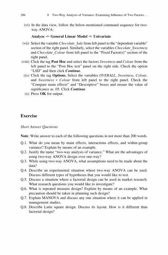
(vi) In the data view, follow the below-mentioned command sequence for two-
way ANOVA:
Analyze ➾ General Linear Model ➾ Univariate
(vii) Select the variable Chocolate_Sale from left panel to the “dependent variable”
section of the right panel. Similarly, select the variables Chocolate_Sweetnessand Chocolate_Colour from left panel to the “Fixed Factor(s)” section of the
right panel.
(viii) Click the tag Post Hoc and select the factors Sweetness and Colour from the
left panel to the “Post Hoc test” panel on the right side. Check the option
“LSD” and then click Continue.(ix) Click the tag Options, Select the variables OVERALL, Sweetness, Colour,
and Sweetness � Colour from left panel to the right panel. Check the
“Compare main effects” and “Descriptive” boxes and ensure the value of
significance as .05. Click Continue.(x) Press OK for output.
Exercise
Short Answer Questions
Note: Write answer to each of the following questions in not more than 200 words.
Q.1. What do you mean by main effects, interactions effects, and within-group
variance? Explain by means of an example.
Q.2. Justify the name “two-way analysis of variance.” What are the advantages of
using two-way ANOVA design over one-way?
Q.3. While using two-way ANOVA, what assumptions need to be made about the
data?
Q.4. Describe an experimental situation where two-way ANOVA can be used.
Discuss different types of hypotheses that you would like to test.
Q.5. Discuss a situation where a factorial design can be used in market research.
What research questions you would like to investigate?
Q.6. What is repeated measure design? Explain by means of an example. What
precaution should be taken in planning such design?
Q.7. Explain MANOVA and discuss any one situation where it can be applied in
management studies.
Q.8. Describe Latin square design. Discuss its layout. How is it different than
factorial design?
286 8 Two-Way Analysis of Variance: Examining Influence of Two Factors. . .
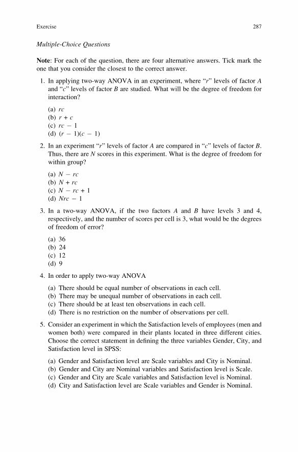
Multiple-Choice Questions
Note: For each of the question, there are four alternative answers. Tick mark the
one that you consider the closest to the correct answer.
1. In applying two-way ANOVA in an experiment, where “r” levels of factor Aand “c” levels of factor B are studied. What will be the degree of freedom for
interaction?
(a) rc(b) r + c(c) rc � 1
(d) (r � 1)(c � 1)
2. In an experiment “r” levels of factor A are compared in “c” levels of factor B.Thus, there are N scores in this experiment. What is the degree of freedom for
within group?
(a) N � rc(b) N + rc(c) N � rc + 1
(d) Nrc � 1
3. In a two-way ANOVA, if the two factors A and B have levels 3 and 4,
respectively, and the number of scores per cell is 3, what would be the degrees
of freedom of error?
(a) 36
(b) 24
(c) 12
(d) 9
4. In order to apply two-way ANOVA
(a) There should be equal number of observations in each cell.
(b) There may be unequal number of observations in each cell.
(c) There should be at least ten observations in each cell.
(d) There is no restriction on the number of observations per cell.
5. Consider an experiment in which the Satisfaction levels of employees (men and
women both) were compared in their plants located in three different cities.
Choose the correct statement in defining the three variables Gender, City, and
Satisfaction level in SPSS:
(a) Gender and Satisfaction level are Scale variables and City is Nominal.
(b) Gender and City are Nominal variables and Satisfaction level is Scale.
(c) Gender and City are Scale variables and Satisfaction level is Nominal.
(d) City and Satisfaction level are Scale variables and Gender is Nominal.
Exercise 287
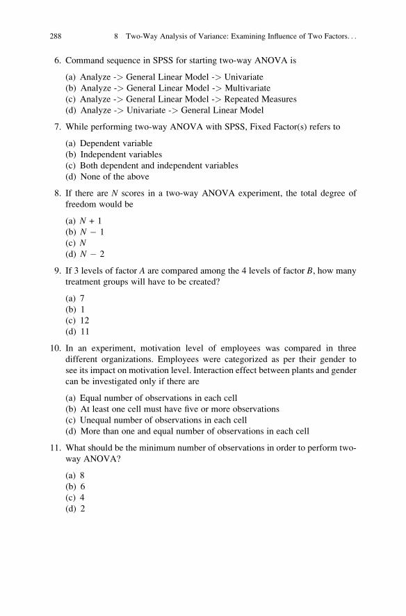
6. Command sequence in SPSS for starting two-way ANOVA is
(a) Analyze -> General Linear Model -> Univariate
(b) Analyze -> General Linear Model -> Multivariate
(c) Analyze -> General Linear Model -> Repeated Measures
(d) Analyze -> Univariate -> General Linear Model
7. While performing two-way ANOVA with SPSS, Fixed Factor(s) refers to
(a) Dependent variable
(b) Independent variables
(c) Both dependent and independent variables
(d) None of the above
8. If there are N scores in a two-way ANOVA experiment, the total degree of
freedom would be
(a) N + 1
(b) N � 1
(c) N(d) N � 2
9. If 3 levels of factor A are compared among the 4 levels of factor B, how many
treatment groups will have to be created?
(a) 7
(b) 1
(c) 12
(d) 11
10. In an experiment, motivation level of employees was compared in three
different organizations. Employees were categorized as per their gender to
see its impact on motivation level. Interaction effect between plants and gender
can be investigated only if there are
(a) Equal number of observations in each cell
(b) At least one cell must have five or more observations
(c) Unequal number of observations in each cell
(d) More than one and equal number of observations in each cell
11. What should be the minimum number of observations in order to perform two-
way ANOVA?
(a) 8
(b) 6
(c) 4
(d) 2
288 8 Two-Way Analysis of Variance: Examining Influence of Two Factors. . .

12. What should be the minimum number of observations in order to perform two-
way ANOVA with interaction effect?
(a) 8
(b) 6
(c) 4
(d) 2
Assignments
1. Four salesmen were appointed by a company to sell their products in door-to-
door marketing. Their sales were observed in three seasons, summer, rainy, and
winter, on month to month basis. The sales data so obtained (in lakhs of rupees)
are shown in the following table:
Discuss your findings by applying two-way ANOVA. Test your hypotheses at
5% level.
2. The management of a private bank was interested to know the stress level of
their employees in different age categories and gender. A stress questionnaire
was administered on the randomly selected employees in different age
categories. The scores on their stress level are shown in the following table:
Apply two-way ANOVA and discuss your findings at 5% level.
Sales data (in lakhs of rupees)
of the sales persons in
different season Season
Salesmen
A B C D
Summer 36 36 21 25
35 32 25 27
32 30 28 24
38 33 25 29
Rainy 26 28 29 29
25 28 32 31
27 31 33 34
29 28 38 39
Winter 28 29 31 32
27 32 35 31
32 33 31 28
29 35 41 33
Exercise 289
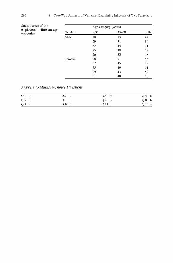
Answers to Multiple-Choice Questions
Q.1 d Q.2 a Q.3 b Q.4 a
Q.5 b Q.6 a Q.7 b Q.8 b
Q.9 c Q.10 d Q.11 c Q.12 a
Stress scores of the
employees in different age
categories Gender
Age category (years)
<35 35–50 >50
Male 28 55 42
29 51 39
32 45 41
25 48 42
26 53 48
Female 28 51 55
32 45 58
35 49 61
29 43 52
31 48 50
290 8 Two-Way Analysis of Variance: Examining Influence of Two Factors. . .

Chapter 9
Analysis of Covariance: Increasing Precision
in Comparison by Controlling Covariate
Learning Objectives
After completing this chapter, you should be able to do the following:
• Learn the concept of analysis of covariance.
• Know the application of analysis of covariance in different situation.
• Describe the concept of covariate and neutralize its effect from the treatment
effect.
• Know the model involved in the analysis of covariance.
• Understand the concept of adjusting treatment means for covariate using linear
regression.
• Understand the analysis of covariance graphically.
• Learn the method of using analysis of covariance.
• Understand as to why the analysis of covariance is efficient design in comparison
to one-way analysis of variance.
• To be able to formulate the hypotheses in analysis of covariance.
• Understand the assumptions used in analysis of covariance.
• Know the method of preparing data file for analysis in SPSS.
• Learn the steps involved in using SPSS for analysis of covariance.
• Interpret the output obtained in analysis of covariance.
• Learn the model way of writing the results of analysis.
Introduction
To compare the effectiveness of two or more treatments on certain criterion
variable, we use one-way analysis of variance technique. This technique has been
discussed in Chap. 7. In testing the comparative effectiveness of different
treatments, the subjects are selected in each experimental group by using the
J.P. Verma, Data Analysis in Management with SPSS Software,DOI 10.1007/978-81-322-0786-3_9, # Springer India 2013
291

principle of randomization. In a situation if the randomization is not possible,
groups are equated on the basis of one or more known parameters. The randomization
or matching is done in order to have the similar initial conditions so that whatever the
changes in criterion variable occurs in the treatment groups can be attributed due to
the treatments only. But in many situations, randomization of subjects or experimen-
tal units may not be possible as the experimenter may be forced to take the two or
more intact samples from different locations due to administrative or financial
constraints. For example, consider an experiment where it is desired to compare the
effect of different types of tariff incentives on the mobile recharge revenue. In this
situation, an experimenter does not have any choice to select the subjects randomly in
different experimental groups. Samples will have to be drawn from the predefined
clientele sets of different mobile companies. In such situations, groups are not
homogeneous initially. These subjects in intact groups may differ in so many ways
which might affect their behavior pattern. Thus, statistical control or indirect proce-
dure is necessary to reduce the experimental error which causes due to such initial
differences in the groups.
In experimental research, the individual variations that appear within the
measures on the criterion variable are potentially correlated with some extraneous
variable. If the criterion variable is a measure of how well subjects learn English
speaking under one or the other of the two methods of instructions, the potential
correlates are likely to include parameters such as prior knowledge of grammar,
motivation level, aptitude, age, and intelligence. These potential correlates are
known as covariates. Analysis of covariance can be used to compare the effective-
ness of these instructional methods on learning English speaking after removing the
effect of the identified covariates.
Introductory Concepts of ANCOVA
Analysis of covariance (ANCOVA) is a statistical technique that may be considered
as an extension of analysis of variance (ANOVA). Analysis of covariance combines
features of one-way analysis of variance with simple linear regression. It is so
because the treatment groups are compared like the way we do in analysis of
variance and we adjust the measurement on criterion variable on the basis of
covariate by using the concept of regression analysis.
In ANCOVA, we try to minimize the error variance by controlling the concomi-
tant variable which varies along with the criterion variable in all the experimental
groups. These concomitant variables are known as covariate. Typically, a covariate
is highly correlated with a criterion variable; that is, the covariate contains infor-
mation about the criterion variable and therefore possibly also explains the differ-
ence in the treatment groups. The purpose in the ANCOVA design is to isolate the
variability component due to covariate so that group difference if any may be solely
attributed to the treatments only. Analysis of covariance is used in a situation where
there is at least one categorical factor and one or more continuous covariates.
292 9 Analysis of Covariance: Increasing Precision in Comparison by Controlling. . .

Since ANCOVA is the combination of ANOVA and regression analysis, this
design can be used with any ANOVA model. One can do a completely randomized
design, randomized block design, a Latin square design, or any other design if a
covariate is put on it. All we need is one measurement for the covariate to go with
every observation. In this chapter, only completely randomized design shall be
discussed as an ANOVA model.
Graphical Explanation of Analysis of Covariance
In order to understand the ANCOVA model, let us first refresh our concept of
representing the line in the slope intercept form. You may recall that this line used
to be represented by
Y ¼ mXþ c (9.1)
where m is the slope and c is the intercept of the line on y-axis. Graphically this
equation can be represented by the Fig. 9.1.
Equation of line in any form may be converted to this slope intercept form for
comparing their slopes and intercepts.
The line shown in Fig. 9.1 is a regression line for estimating the value of Y if
the value of X is known. Now if you look at the vertical line over �x, it intersectsthe regression line at (�x and �y). In other words, the point (�x, �y) actually lies on the
regression line. This concept shall be used to explain the analysis of covariance.
To understand ANCOVA, let us consider A and B represent the two treatments.
Further, YA and YB represent the value of criterion variable, whereas XA and XB
represent the value of covariate in the two treatment groups A and B respectively.
These two treatments are represented by the lines A and B in Fig. 9.2. If higher value
( x , y)y
C Y= mX + c
x
Fig. 9.1 Regression equation
of Y on X
Graphical Explanation of Analysis of Covariance 293

of Y indicates better performance, then obviously treatment A would be better
treatment because the line A is higher everywhere than line B.
But sometimes corresponding to very low value of XB and very high value of XA,
the values ofYB is higher thanYA. This can mislead the researcher. If line B is always
higher than line A, then the sample means end up reversed. The difference observed
inY0s is not because of the treatments but due to the covariate means (X
0s) which are
so apart.
In analysis of covariance, what we do is to compare the values of YA and YB at �X
(overall grand mean of XA and XB). Now the distance between the two curves is the
same because the lines are parallel. What we do here is to adjust both means so that
we are evaluating the points of the same X on the curves. In this way, we get a more
balanced comparison.
If treatments are compared without using ANCOVA, what may happen? Sup-
pose the above-mentioned lines A and B are exactly the same, still Yi ’s may be
different. This may be because the effect of one treatment is observed at higher
average covariate mean and the other treatment effect is measured with lower
average covariate mean. This fact may not be revealed if the analysis of covariance
is not done. Thus, in analysis of covariance, we compare the effect of treatments
mean (Yi’s) by adjusting them with the average covariate means ( �X).
Analysis of Covariance Model
If Yij represents the jth score of the criterion variable in the ith treatment group and
Xij represents the jth score of the covariate in the ith treatment group, then the one-
way ANCOVA model is represented as follows:
Yij ¼ mþ bðXij � �XÞ þ eij (9.2)
Fig. 9.2 Geometrical representation of two treatments (Y’s) with their covariates (X’s)
294 9 Analysis of Covariance: Increasing Precision in Comparison by Controlling. . .

where
m is the overall population mean (on criterion variable)
b is slope of the lines
�X is combined mean of the covariate in all the treatment groups
eij is unexplained error terms which are independent and normally distributed with
mean 0 and variance 1
One-way analysis of covariance fits a straight line to each treatment group of X-Ydata, such that the slopes of the lines are all equal. This fitted model may then be
used to test the following null hypothesis:
H0: The intercepts for each line are equal.
This hypothesis tests as to whether all the treatment group means are equal or not
after making the adjustment for X (covariate). Here, we assume that the slopes are
equal. It is so because there is no point of comparing the treatments effect if one of
the treatments produces positive effect whereas other induces negative effect.
Let us see how the treatment means are adjusted for covariate and are computed
for comparison. Adding both sides of Eq. (9.2) for j and dividing by n (number of
scores in each treatment group), we get
1
n
Xj
Yij ¼ mþ b1
n
Xj
Xij � �X
!þ 1
n
Xj
eij
) Yi ¼ mþ bðXi � �XÞ þ �ei
Since mean of ei is zero, the equation becomes
Yi ¼ mþ bðXi � �XÞ (9.3)
where
Yi is mean of the criterion variable in the ith treatment group
m is the overall population mean (on criterion variable)
Xi is mean of the covariate (X data) in the ith treatment group
Other symbols have their usual meanings. If one-way ANCOVA model has two
treatment groups, then the model (9.3) will give rise to two straight lines as shown
in Fig. 9.2. Thus, by testing the hypothesis H0 in ANCOVA, we actually compare
the two treatments YA and YB after adjusting it for the covariates.
Analysis of Covariance Model 295
Remark
1. If the slope of line A and B is equal it indicates that the effect of both the
treatments are in one direction only. Both the treatments will induce either
positive or negative effect.
2. By comparing the intercepts of the lines, we try to compare whether the effect of
all the treatments on the criterion variable is same or not.
What We Do in Analysis of Covariance?
In analysis of covariance, the purpose of the analysis is to compare the posttreat-
ment means of the groups by adjusting the initial variations in the grouping. The
statistical control is achieved by including measures on supplementary or concom-
itant variate (X) in addition to the variate of primary interest (Y) after implementing
the treatments. The concomitant variate that may not be of experimental interest is
called covariate and designated as X. Let us designate the variable which is of
interest in the experiment as Y, also known as criterion variable. Thus, in
ANCOVA, we have two observations (X and Y) from each subject. Measurements
on X (covariate) are obtained prior to the administration of treatments and are
primarily to adjust the measurements on Y (criterion). Covariate is the variable
which is assumed to be associated with the criterion variable. When X and Y are
associated, a part of the variability of Y is due to the variation in X. If the value ofcovariate X is constant over the experimental units, there would be corresponding
reduction in the variance of Y.Let us consider an example in which the analysis of covariance can be applied to
reduce the estimate of experimental error. Suppose an experiment is conducted to
study the effect of three different types of advertising campaign on the sale of a
product. Further, the experimenter is forced to use three intact groups of outlets from
three different states. However, there is a freedom to assign groups randomly to the
treatment conditions (types of advertisement). Out of three groups, one may serve as
control. Since the subjects cannot be assigned randomly to the treatment groups, the
possibility of initial differences (before administration of treatment) among the
groups always exist. Thus, one may decide to record the sale of each outlet (X)before applying the treatments, which serves as a measure of covariate. This measure
of covariate is used to adjust the post advertisement sale figure (Y) in different outlets.The Y is the sale of the product which is obtained after the implementation of the
treatments (advertisements).
Thus, the variates X and Y can be defined as follows:
X ¼ sale of the product on 15 consecutive days in each experimental groups before
treatments (advertisements).
296 9 Analysis of Covariance: Increasing Precision in Comparison by Controlling. . .

Y ¼ sale of the product on 15 consecutive days in each experimental groups after
treatments (advertisements).
In general, if Y measures (criterion) are substantially correlated with Xmeasures (covariate), the analysis of covariance will result in similar estimate
of experimental error than would be obtained from the analysis of variance.
Thus, in ANCOVA, the following null hypothesis is tested
H0 : mAdj Post Adv 1 ¼ mAdj Post Adv 2 ¼ mAdj Post Control
against the possible alternatives that at least one group mean differs
where
Adj_Post_Adv_1 is adjusted mean sale in the first treatment group (where first
advertisement campaign was used)
Adj_Post_Adv_2 is adjusted mean sale in the second treatment group (where
second advertisement campaign was used)
Adj_Post_Adv_3 is adjusted mean sale in the third treatment group (where no
advertisement campaign was used)
ANCOVA table generated in the SPSS output contains the value of F-statisticsalong with their significance value. Thus, if F-value is significant, the null
hypothesis is rejected and the post hoc test is used to compare the adjusted
posttreatment means of different groups in pairs.
When to Use ANCOVA
The analysis of covariance is used to test the comparative effectiveness of two or
more treatments on the criterion variable after adjusting for their initial
differences due to covariate. The covariate should be identified before the experi-
ment, and its value should be measured on each of the experimental units. In many
situations, it is not possible to identify single covariate which affects the measure
on criterion variable during experimentation. In that case, initial testing (X) on thecriterion variable in each of the treatment group may be considered as covariate,
and the measure on the criterion variable after the treatment (Y) in all the
treatment groups is the one in which we are interested to investigate. The analysis
of covariance design should be used if the following things happen:
(a) The response on the criterion variable is continuous.
(b) There are one or more classification variables (treatment groups).
(c) There are one or more continuous independent variables (covariate).
When to Use ANCOVA 297

Assumptions in ANCOVA
In using the analysis of covariance design following assumptions are made:
1. The criterion variable must have the same variance in each of the treatment
groups.
2. The data on criterion variable must have been obtained randomly.
3. The interaction between the criterion variable and covariate is negligible. The
adjusted mean of the criterion variable in each of the treatment groups is
computed owing to this assumption. If this assumption is violated, then the
adjustment of the criterion variable to a common value of the covariate will be
misleading.
4. Since ANCOVA uses the concept of linear regression, the assumption of
linearity between independent and dependent variable must hold true.
5. The regression coefficients (slope) for each treatment groups must be homo-
geneous. If this assumption is violated, then the ANCOVA results will be
misleading.
Efficiency in Using ANCOVA over ANOVA
The ANCOVA design is more efficient in comparison to one-way ANOVA. It is
because of the fact that in ANCOVA, a part of the variability due to error
component is defined by the covariate and, hence, the error variance reduces
comprehensively in comparison to one-way ANOVA design. In one-way
ANOVA, the total variability is split into two components, that is, between groups
and within groups. Here, the variability due to covariate is confounded into error
component, and, hence, this design is inferior to ANCOVA in a situation where the
covariate effects the measurement on criterion variable. In fact, one-way ANOVA
should be used only in a situation where it is known that all the treatment groups are
homogenous in all respect and perfect control is observed during the entire period
of experimentation.
Solved Example of ANCOVA Using SPSS
Example 9.1 A study was planned to investigate the effect of different doses of
vitamin C in curing the cold. Forty five subjects who were suffering from cold
symptoms were divided into three groups. The first two groups were given a low
dose and high dose of vitamin C every day whereas the third group was given a
placebo. The number of days these subjects were suffering from cold before starting
the treatment was taken as the covariate whereas the curing time in each treatment
group was recorded as a dependent variable. The data so obtained on the subjects
are shown in the Table 9.1.
298 9 Analysis of Covariance: Increasing Precision in Comparison by Controlling. . .

Apply analysis of covariance to see as to which dose of vitamin C is more effective
in controlling cold. Test your hypothesis at 5% level of significance.
Solution In this example, the variables are as follows:
Treatments: The three treatments are as follows:
Treatment A: Administering high dose of vitamin C
Treatment B: Administering low dose of vitamin C
Treatment C: Administering placebo
Covariate: The number of days having cold symptoms before treatment.
Dependent Variable: Curing time of cold symptomsHere, it is required to compare the average curing time among the three treat-
ment groups, that is, high dose of vitamin C, low dose of vitamin C, and placebo,
after adjusting for the covariate (average number of days having cold symptoms
before treatments).
Thus, the following null hypothesis needs to be tested
H0 : mAdj Days in Treatment A ¼ mAdj Days in Treatment B ¼ mAdj Days in Treatment C
against the alternative hypothesis that at least one group mean (adjusted) is different
Table 9.1 Data on cold duration before and during implementation of vitamin C in different
groups
Contents of vitamin C
S.N. High dose Low dose Placebo
Pre days Post days Pre days Post days Pre days Post days
1 0 2 14 12 1 10
2 10 3 16 13 10 8
3 11 5 5 8 5 14
4 15 9 12 10 6 9
5 6 3 0 1 10 13
6 12 8 8 4 5 11
7 9 7 12 9 12 15
8 13 7 5 10 13 15
9 1 6 19 10 6 10
10 8 13 14 8 19 20
11 7 12 6 11 8 12
12 6 10 8 11 8 14
13 4 3 5 8 6 12
14 3 2 2 6 5 9
15 4 3 4 6 8 14
Pre days: Cold duration before treatment
Post days: Cold duration during treatment
Solved Example of ANCOVA Using SPSS 299
where
mAdj Days in Treatment A is adjusted mean curing time in treatment group A
mAdj Days in Treatment B is adjusted mean curing time in treatment group B
mAdj Days in Treatment C is adjusted mean curing time in treatment group C
The SPSS output provides ANCOVA table along with pairwise comparison of
adjusted post means of different treatment groups. The pairwise comparison of
means is done only when the F-ratio is significant.
The analysis of covariance table generated in the SPSS output looks similar
to the one- way ANOVA table as only adjusted post means is compared here.
In the ANCOVA table, F-value is shown along with its significance value
(p-value). The F-value would be significant if its corresponding p-value is less
than .05, and in that case null hypothesis would be rejected. Once the F-valueis found to be significant, then a post hoc test is used to compare the paired
means. SPSS provides the choice of post hoc test to be used in the analysis.
In this example, since the sample sizes are equal, LSD test shall be used
as a post hoc test for comparing the group means. The SPSS output provides
the significance value (p-value) for each pair of difference of group
means. Thus, by looking at the values of means, the best treatment may be
identified.
Computations in ANCOVA Using SPSS
(a) Preparing data fileBefore using SPSS commands to solve the problem of analysis of covariance, a
data file needs to be prepared. The following steps will help you prepare the
data file:
(i) Starting the SPSS: Follow the below-mentioned command sequence to start
SPSS:
Start ! Programs ! IBM SPSS Statistics ! IBM SPSS Statistics 20
After clicking the Type in Data, you will be taken to the Variable View
option for defining variables in the study.
(ii) Defining variablesIn this example, three variables, vitamin dose, cold duration before
treatment and cold duration during treatment need to be defined. The
procedure of defining these variables along with their characteristics is
as follows:
300 9 Analysis of Covariance: Increasing Precision in Comparison by Controlling. . .

1. Click the Variable View to define the variables and their properties.
2. Write short name of the variables as Vitamin_Dose, Pre_Days and
Post_Days under the column heading Name.
3. Under the column heading Label, define full name of these variables as
Vitamin dose, Cold duration before treatment, and Cold duration duringtreatment. Other names may also be chosen for describing these
variables.
4. Under the column headingMeasure, select the option “Nominal” for the
variable Vitamin dose and “Scale” for the variables Cold duration beforetreatment and Cold duration during treatment.
5. For the variable Vitamin dose, double-click the cell under the column
Values and add the following values to different labels:
Value Label
1 Treatment A
2 Treatment B
3 Treatment C
6. Use default entries in rest of the columns.
After defining the variables in variable view, the screen shall look as shown
in Fig. 9.3.
(iii) Entering data: After defining all the variables in the Variable View, click
Data View on the left corner in the bottom of the screen shown in Fig. 9.3 to
open the format for entering the data column wise. After entering the data,
the screen will look like Fig. 9.4. Save the data file in the desired location
before further processing.
Fig. 9.3 Defining variables and their characteristics
Solved Example of ANCOVA Using SPSS 301

Fig. 9.4 Screen showing
entered data for all the
variables in the data view
302 9 Analysis of Covariance: Increasing Precision in Comparison by Controlling. . .

(b) SPSS commands for ANCOVAAfter preparing the data file, do the following steps for analysis of covariance:
(i) Initiating the SPSS commands for ANCOVA: In data view, click the follow-ing commands in sequence:
Analyze ) General Linear Model ) Univariate
The screen shall look like Fig. 9.5.
(ii) Selecting variables for ANCOVA: After clicking the Univariate option,
you will be taken to the next screen as shown in Fig. 9.6 for selecting
variables. Select the variables as follows:
– Cold duration during treatment from left panel to the “Dependent
variable” section of the right panel.
– Vitamin dose from left panel to the “Fixed Factor(s)” section of the right
panel.
– Cold duration before treatment from the left panel to the “Covariate(s)”
section of the right panel.
(iii) Selecting the options for computation: After selecting the variables, dif-
ferent options need to be defined for generating the output in ANCOVA.
This shall be done as follows:
– Click the tag Model on the screen shown in Fig. 9.6 and do the
following:
– Select the sum of squares option as “Type I.”
– Press Continue.
Fig. 9.5 Sequence of SPSS commands for analysis of covariance
Solved Example of ANCOVA Using SPSS 303
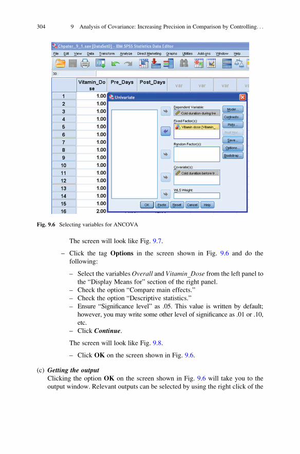
The screen will look like Fig. 9.7.
– Click the tag Options in the screen shown in Fig. 9.6 and do the
following:
– Select the variables Overall and Vitamin_Dose from the left panel to
the “Display Means for” section of the right panel.
– Check the option “Compare main effects.”
– Check the option “Descriptive statistics.”
– Ensure “Significance level” as .05. This value is written by default;
however, you may write some other level of significance as .01 or .10,
etc.
– Click Continue.
The screen will look like Fig. 9.8.
– Click OK on the screen shown in Fig. 9.6.
(c) Getting the outputClicking the option OK on the screen shown in Fig. 9.6 will take you to the
output window. Relevant outputs can be selected by using the right click of the
Fig. 9.6 Selecting variables for ANCOVA
304 9 Analysis of Covariance: Increasing Precision in Comparison by Controlling. . .

mouse and may be copied in the word file. The identified outputs shall be
rearranged for interpreting the findings. The details have been shown under the
heading Model Way of Writing the Results.
(d) SPSS outputThe readers should note the kind of outputs to be selected from the output
window of SPSS for explaining the findings. The following four outputs have
been selected for discussing the results of ANCOVA:
1. Descriptive statistics
2. Adjusted estimates of the dependent variable
3. ANCOVA table
4. Post hoc comparison table
These outputs have been shown in Tables 9.2, 9.3, 9.4, and 9.5.
Fig. 9.7 Screen showing option for choosing sum of squares and model type
Solved Example of ANCOVA Using SPSS 305

Table 9.2 Descriptive
statisticsVitamin dose Mean Std. deviation N
Treatment A 6.2000 3.62925 15
Treatment B 8.4667 3.18179 15
Treatment C 12.4000 3.11219 15
Total 9.0222 4.14778 45
Dependent variable: Cold duration during treatment
Table 9.3 Adjusted estimates
Vitamin dose Mean Std. error
95% Confidence interval
Lower bound Upper bound
Treatment A 6.508a .704 5.086 7.930
Treatment B 8.204a .703 6.784 9.625
Treatment C 12.355a .701 10.939 13.771
Dependent variable: Cold duration during treatmentaCovariates appearing in the model are evaluated at the following values: Cold duration before
treatment ¼ 8.0222
Fig. 9.8 Selecting options for ANCOVA output
306 9 Analysis of Covariance: Increasing Precision in Comparison by Controlling. . .

Model Way of Writing the Results of ANCOVA
and Their Interpretations
The above output generated by the SPSS can be shown in a much more user-
friendly format by modifying the relevant contents of the Tables 9.2, 9.3, 9.4, and
9.5. The below-mentioned edited outputs can directly be shown in the project,
dissertation, or thesis. These modified outputs shall be used to discuss the findings
of ANCOVA.
(a) Descriptive Statistics of the Data Obtained on the Criterion VariableThe mean and standard deviation of the criterion variable in different treatment
groups have been shown in Table 9.6. Entries in this table have been copied
from Table 9.2. If you are interested in computing different descriptive statistics
for the covariate (Number of days having cold symptoms before treatment)
also, the same be computed by using the procedure discussed in Chap. 2.
However, the SPSS does not generate these statistics during ANCOVA
analysis.
Look at the table heading which can be used in writing the final results in
your study.
Table 9.4 Tests “between-subjects” effects
Source Type I sum of squares df Mean square F Sig.
Corrected model 454.761a 3 151.587 20.565 .000
Intercept 3,663.022 1 3,663.022 496.941 .000
Pre_Days 183.993 1 183.993 24.961 .000
Vitamin_Dose 270.768 2 135.384 18.367 .000
Error 302.217 41 7.371
Total 4,420.000 45
Corrected total 756.978 44
Dependent variable: Cold duration during treatmentaR squared ¼ .601 (adjusted R squared ¼ .572)
Table 9.5 Pairwise comparisons
(I) Vitamin dose (J) Vitamin dose Mean diff. (I–J) SE Sig.a
95% Confidence interval for
differencea
Lower bound Upper bound
Treatment A Treatment B �1.697 .999 .097 �3.714 .321
Treatment C �5.847* .994 .000 �7.855 �3.839
Treatment B Treatment A 1.697 .999 .097 �.321 3.714
Treatment C �4.151* .992 .000 �6.155 �2.146
Treatment C Treatment A 5.847* .994 .000 3.839 7.855
Treatment B 4.151* .992 .000 2.146 6.155
Dependent variable: Cold duration during treatment
Based on estimated marginal means
*The mean difference is significant at the .05 levelaAdjustment for multiple comparisons: Least significant difference (equivalent to no adjustments)
Model Way of Writing the Results of ANCOVA and Their Interpretations 307

From Table 9.6, it can be seen that average time taken to cure the cold
symptoms is highest in treatment group C whereas the least time is in treatment
group A. Treatment C signifies the placebo, whereas treatment A is the high
dose of vitamin C. The next question is to see whether this difference is
significant or not after adjusting for the covariate (number of days having
cold symptoms before treatment).
(b) Descriptive Statistics of the Data Obtained on the Criterion Variable afterAdjusting for CovariateThe adjusted mean and standard error of the criterion variable in different
treatment groups have been shown in Table 9.7. The mean of criterion variable
has been obtained in all the three treatment groups after adjusting for the
covariate (Number of days having cold symptoms before treatment). These
data have been taken from Table 9.3. Readers may note that these values are
different from that of the unadjusted values shown in Table 9.6. The advantage
of using the ANCOVA is that the differences in the posttesting means are
compensated for the initial differences in the scores. In other words, it may be
said that the effect of covariate is eliminated in comparing the effectiveness of
treatments on the criterion variable.
Kindly note the heading of the table which may be used for writing the final
results of ANCOVA.
(c) ANCOVA Table for the Data on Criterion Variable (Number of Days HavingCold Symptoms During Treatment)The main ANCOVA table may be reproduced by deleting some of the
unwanted details of Table 9.4. The final results of ANCOVA have been
shown in Table 9.8. The “significance” (Sig.) value has been named as p-value. In most of the scientific literature, p-value is used instead of term
significance value.
Table 9.6 Mean and
standard deviation of cold
duration in different groups
during treatment
Vitamin dose Mean Std. deviation N
Treatment A 6.2 3.6 15
Treatment B 8.5 3.2 15
Treatment C 12.4 3.1 15
Total 9.0222 4.14778 45
Values have been rounded off
Table 9.7 Adjusted mean and standard error for the data on cold duration in different groups
during treatment
Vitamin dose Mean Std. error
95% Confidence interval
Lower bound Upper bound
Treatment A 6.5a .70 5.09 7.93
Treatment B 8.2a .70 6.78 9.63
Treatment C 12.4a .70 10.94 13.77aCovariates appearing in the model are evaluated at the following values:
Cold duration before treatment ¼ 8.0222
Values have been rounded off
308 9 Analysis of Covariance: Increasing Precision in Comparison by Controlling. . .

Table 9.8 shows the F-value for comparing the adjusted means of the criterion
variable in three Vitamin_Dose groups (treatment A, treatment B, and treatment
C). You can note that F-statistic computed for Vitamin_Dose is significant
because p -value associated with it is .000 which is less than .05. Thus, the null
hypothesis of no difference among the adjusted means for the data on criterion
variable (number of days having cold symptoms during treatment) in three
treatment groups may be rejected at 5% level.
Remark: You can see that the F-value for Pre_Days (covariate) is also signifi-
cant. It shows that the initial conditions of the experimental groups are not
same, and that is why we are applying ANCOVA after adjusting mean values of
the criterion variable for the covariate.
(d) Post Hoc Comparison for the Group Means in Post-measurement Adjustedwith the Initial DifferencesSince F-statistic is significant, post hoc comparison has been made for the
adjusted means of the three treatment groups, which is shown in Table 9.9.
This, table has been obtained by deleting some of the information from
Table 9.5. It may be noted here that p-value for the mean difference between
treatments A and C as well between treatments B and C is .000. Since p value isless than .05, both these mean differences are significant at 5% level. Thus, the
following conclusions can be drawn:
(i) There is a significant difference between the adjusted means of criterion
variable (Number of days having cold symptoms during treatment) in
treatment A (High vitamin C dose) and treatment C (Placebo).
Table 9.8 ANCOVA table for the data on cold duration in different groups during treatment
Source Sum of squares df Mean square F (p-value) Sig.
Pre_Days 183.993 1 183.993 24.961 .000
Vitamin_Dose 270.768 2 135.384 18.367 .000
Error 302.217 41 7.371
Corrected total 756.978 44
Table 9.9 Pairwise comparisons
(I) Vitamin dose (J) Vitamin dose Mean diff. (I–J) (p-value) Sig.a
Treatment A Treatment B �1.697 .097
Treatment C �5.847* .000
Treatment B Treatment A 1.697 .097
Treatment C �4.151* .000
Treatment C Treatment A 5.847* .000
Treatment B 4.151* .000
Dependent variable: Cold duration during treatment
Based on estimated marginal means
*The mean difference is significant at the .05 levelaAdjustment for multiple comparisons: Least significant difference (equivalent to no adjustments)
Model Way of Writing the Results of ANCOVA and Their Interpretations 309

(ii) There is a significant difference between the adjusted means of criterion
variable (Number of days having cold symptoms during treatment) in
treatment B (Low vitamin C dose) and treatment C (Placebo).
(iii) There is no significant difference between the adjusted means of criterion
variable (Number of days having cold symptoms during treatment) in
treatment A (High vitamin C dose) and treatment B (Low vitamin dose).
In order to find as to which treatment is the best, one can see the adjusted mean
values of criterion variable in different treatment groups given in Table 9.7. Club-
bing these adjusted means with the three conclusions mentioned above, one may get
the answer. However, this task becomes much easier if Table 9.10 is developed.
This table can be created by using the values of different adjusted group means from
Table 9.7 and using p-values of mean differences from Table 9.9. In this table,
the adjusted means of the criterion variable in different treatment groups have
been shown in the descending order. If the difference between any two group
means is significant (which can be seen from Table 9.10), nothing is done, and if
the mean difference is not significant, an underline is put below both the group
means.
Thus, it may be concluded that the average curing time in high and low vitamin
groups was same. Further, the average curing time in both these groups was
significantly less than that of placebo group.
Hence, it may be inferred that high vitamin dose as well as low vitamin dose are
equally effective in curing the cold symptoms in comparison to that of placebo.
Summary of the SPSS Commands
(i) Start the SPSS by using the following commands:
Start ! Programs ! IBM SPSS Statistics ! IBM SPSS Statistics 20
Table 9.10 Post hoc
comparison of adjusted means
in different groups for the data
on cold duration during
treatment with graphics
Treatment C Treatment B Treatment A
12.4 8.2 6.5
“ ” represents no significant difference between the means
Treatment A: Administering high dose of vitamin C
Treatment B: Administering low dose of vitamin C
Treatment C: Administering placebo
310 9 Analysis of Covariance: Increasing Precision in Comparison by Controlling. . .
(ii) Click Variable View tag and define the variables Vitamin_Dose as nominal
variable and Pre_Days and Post_Days as scale variables.(iii) Under the column heading Values against the variable Vitamin_Dose,
define “1” for Treatment A, “2” for Treatment B, and “3” for Treatment C.(iv) After defining the variables, type the data for these variables by clicking
Data View.
(v) In the data view, follow the below-mentioned command sequence for
ANCOVA:
Analyze ) General Linear Model ) Univariate
(vi) Select the variables Cold duration during treatment, Vitamin dose, and Coldduration before treatment from left panel to the “Dependent variable”
section, “Fixed Factor(s)” section, and “Covariate(s)” section of the right
panel, respectively.
(vii) Click the tagModel and select the Sum of Squares option as “Type I.” Press
Continue.(viii) Click the tag Options and select the variables Overall and Vitamin_Dose
from the left panel to the “Display Means for” section of the right panel.
Check the option “Compare main effects” and “Descriptive statistics.”
Ensure the value of significance as .05 or .01 as the case may be. Press
Continue.(ix) Click OK for output.
Exercise
Short Answer Questions
Note:Write answer to each of the following questions in not more than 200 words.
Q1. What do you mean by the covariate? How it is controlled in ANCOVA? Give
a specific example.
Q2. Describe an experimental situation where ANCOVA can be applied. Construct
null hypothesis and all possible alternative hypotheses.
Q3. Thirty boys were selected for direct marketing of a vacuum cleaner in three
similar cities. In each of the city, 10 boys were sent for direct marketing for a
month. Three different kinds of incentives, namely, conveyance allowance,
two percent bonus, and gifts were offered to these sales agents in these three
cities on completing the target. To compare the effectiveness of three different
incentives on sale, which statistical technique should be used?
Q4. If two treatment groups are to be compared on some criterion variable, how do
you interpret if the slopes of the two regression lines are same? Further, if the
intercepts are equal, what it conveys? Explain by means of graphical
representation.
Exercise 311

Q5. Explain the statement “the analysis of covariance is a mix of one-way ANOVA
and linear regression.”
Q6. Why the observed mean of criterion variable is adjusted in ANCOVA? How
this adjustment is done?
Q7. What are the various assumptions used in analysis of covariance?
Q8. Which design is more efficient and why among one-way ANOVA and
ANCOVA?
Multiple-Choice Questions
Note: For each of the question, there are four alternative answers. Tick mark the
one that you consider the closest to the correct answer.
1. In designing an experiment, if the randomization is not possible, control
is observed by matching the groups. This matching is done on the variable
which is
(a) Independent
(b) Extraneous
(c) Dependent
(d) Any variable found suitable
2. Covariate is a variable which is supposed to be correlated with
(a) Criterion variable
(b) Independent variable
(c) Dependent variable
(d) None of the above
3. In ANCOVA, while doing post hoc analysis, which group means are
compared?
(a) Pretest group means
(b) Posttest group means
(c) Pretest adjusted group means
(d) Posttest adjusted group means
4. In ANCOVA, if the slopes of the regression lines in different treatment groups
are same, one can infer that
(a) Some of the treatments will show the improvement where the other
treatments may show the deterioration.
(b) All the treatments will show either deterioration or improvement but with
varying degrees.
(c) One cannot tell about the improvement or deterioration due to different
treatments.
(d) All treatments will have the same amount of improvement in the criterion
variable.
5. In ANCOVA, if intercepts of the regression lines in the two treatment groups
are same, then it may be inferred that
312 9 Analysis of Covariance: Increasing Precision in Comparison by Controlling. . .

(a) One treatment is better than other.
(b) One cannot say which treatment is more effective.
(c) Both the treatments are equally effective.
(d) No conclusion can be drawn.
6. In ANCOVA model, the error component is independently and identically
normally distributed with
(a) Mean 0 and variance 1
(b) Mean 1 and variance 0
(c) Equal mean and variance 1
(d) Mean 0 and equal variance
7. In ANCOVA, the adjusted mean m in the ith treatment group is obtained from
the formula
(a) m ¼ Yi þ bðXi � �XÞ(b) m ¼ Yi � bðXi � �XÞ(c) m ¼ Yi � bð �X � XiÞ(d) m ¼ Yi þ bþ ðXi � �XÞ
8. In analysis of covariance, the criterion variable should be
(a) Continuous
(b) Nominal
(c) Ordinal
(d) Dichotomous always
9. One of the assumptions in using ANCOVA is
(a) The data on criterion variable must have been obtained by stratified
sampling.
(b) The regression coefficients for each treatment groups must be
heterogeneous.
(c) The interaction between the criterion variable and covariate is significant.
(d) The criterion variable must have the same variance in each of the treatment
groups.
10. Choose the correct statement.
(a) The ANCOVA is more efficient than ANOVA because part of the error
variance is explained by the covariate.
(b) ANOVA is more efficient than ANCOVA if the initial conditions are not
same.
(c) ANOVA and ANCOVA are equally effective, and it is the matter of choice
as to which analysis is to be used.
(d) All the above statements are correct.
11. In order to compare the effectiveness of three training programs on financial
knowledge, an experiment was planned. Three groups of employees were
Exercise 313
tested for their financial knowledge before and after the training program.
While using SPSS for ANCOVA, three variables, namely, Pre_Knowledge
Drib, Post_Knowledge, and Treatment_Group, need to be defined. Choose
the correct types of each variable.
(a) Pre_Knowledge and Post_Knowledge are Scale and Treatment_Group is
Ordinal.
(b) Pre_Knowledge and Post_Knowledge are Nominal and Treatment_Group
is Scale.
(c) Pre_Knowledge and Treatment_Group are Scale and Post_Knowledge is
Nominal.
(d) Pre_Knowledge and Post_Knowledge are Scale and Treatment_Group is
Nominal.
12. While using SPSS for ANCOVA, the three variables, namely, Pre_Test, Post_-
Test, and Treatment_Group, are classified as
(a) Post_Test as Dependent variable whereas Pre_Test and Treatment_Group
as Fixed Factor(s)
(b) Post_Test as Dependent variable, Pre_Test as Covariate, and
Treatment_Group as Fixed Factor
(c) Treatment_Group as Dependent variable, Pre_Test and Post_Test as Fixed
Factor(s)
(d) Treatment_Group as Dependent variable, Post_Test as Covariate, and
Pre_Test as Fixed Factor
13. Choose the correct sequence of commands in SPSS for starting ANCOVA.
(a) Analyze ! Univariate ! General Linear Model
(b) Analyze ! General Linear Model ! Multivariate
(c) Analyze ! General Linear Model ! Univariate
(d) Analyze ! General Linear Model ! Repeated Measures
Assignments
1. In a psychological experiment 60, subjects were randomly divided into three
equal groups. These groups were taught with audiovisual aid, traditional method,
and need-based methods. Prior to the treatments, learning motivation of all the
subjects was assessed. After 4 weeks, improvement in academic achievements
was noted. The data so obtained on academic achievements is shown in the
Table A-1.
Apply analysis of covariance to see as to which methodology of teaching is more
effective for academic achievement. Test your hypothesis at .05 as well as .01
level of significance.
2. A study was conducted to know the impact of gender on life optimism. Since age
is considered as factor effecting life optimism, it was considered as covariate.
314 9 Analysis of Covariance: Increasing Precision in Comparison by Controlling. . .

Table A-1 Scores on academic achievements and learning motivation in three types of teaching
methods
S.N. Audiovisual group Traditional group Need-based group
Motivation Achievement Motivation Achievement Motivation Achievement
1 2 5 2 3 1 12
2 1 10 3 3 3 18
3 3 12 1 9 2 11
4 0 14 1 13 6 25
5 1 14 4 13 3 9
6 5 16 5 13 5 18
7 3 18 6 13 3 12
8 4 18 1 15 4 10
9 4 18 2 15 3 11
10 5 18 4 17 6 16
11 2 22 6 17 7 18
12 3 22 5 21 4 14
13 7 28 2 22 3 17
14 4 24 5 22 2 10
15 6 24 5 22 5 19
16 3 26 5 22 3 14
17 4 26 5 22 2 16
18 4 26 6 20 3 15
19 8 26 9 22 4 16
20 3 29 4 24 5 15
Table A-2 Data on age
and life optimism of the
male and female S.N.
Male Female
Age Life optimism Age Life optimism
1 53 18 20 26
2 38 26 24 15
3 18 20 18 16
4 26 27 38 17
5 39 19 35 16
6 38 29 25 24
7 30 15 17 10
8 60 23 19 18
9 22 22 21 19
10 31 14 19 19
11 21 14 18 21
12 25 23 38 13
13 22 23 37 15
14 20 19 21 11
15 27 23 20 11
16 24 20 20 14
17 29 18 41 16
18 27 19 40 17
19 32 13 28 17
20 17 14 99 8
Exercise 315

A questionnaire was administered on 20 male and 20 female subjects to know
their life optimism. Their age was also noted. The data so obtained are listed in
the Table A-2.
Apply analysis of covariance and discuss your findings to compare the life
optimism among male and female adjusted for their age. Test your hypothesis at
5% as well as at 1% level.
Answers to Multiple-Choice Questions
Q.1 b Q.2 a Q.3 d
Q.4 b Q.5 c Q.6 d
Q.7 b Q.8 a Q.9 d
Q.10 a Q.11 d Q.12 b
Q.13 c
316 9 Analysis of Covariance: Increasing Precision in Comparison by Controlling. . .
Chapter 10
Cluster Analysis: For Segmenting the Population
Learning Objectives
After completing this chapter, you should be able to do the following:
• Understand the concept of cluster analysis.
• Know the different terminologies used in cluster analysis.
• Learn to compute different distances used in the analysis.
• Understand different techniques of clustering.
• Describe the assumptions used in the analysis.
• Explain the situations where cluster analysis can be used.
• Learn the procedure of using cluster analysis.
• Know the use of hierarchical cluster analysis and K-means cluster analysis.
• Describe the situation under which two-step cluster should be used.
• Understand various outputs of cluster analysis.
• Know the procedure of using cluster analysis with SPSS.
• Understand different commands and its outcomes used in SPSS for cluster
analysis.
• Learn to interpret the outputs of cluster analysis generated by the SPSS.
Introduction
Market analysts are always in search of strategies responsible for buying behavior.
The whole lot of customers can be grouped on the basis of their buying behavior
patterns. This segmentation of customers helps analysts in developing marketing
strategy for different products in different segments of customers. These segments
are developed on the basis of buying behavior of the customers in such a way so
that the individuals in the segments are more alike but the individuals in different
segments differ to a great extent in their characteristics. The concept of segmenting
may be used to club different television serials into homogeneous categories on
the basis of their characteristics. An archaeological surveyor’s may like to cluster
different idol excavated from archaeological digs into the civilizations from which
J.P. Verma, Data Analysis in Management with SPSS Software,DOI 10.1007/978-81-322-0786-3_10, # Springer India 2013
317

they originated. These idols may be clustered on the basis of their physical and
chemical parameters to identify their age and civilization to which they belong.
Doctors may diagnose a patient for viral infection and determine whether distinct
subgroups can be identified on the basis of a clinical checklist and pathological
tests. Thus, in different fields several situations may arise where it is required to
segment the subjects on the basis of their behaviour pattern so that an appropriate
strategy may be formed for these segments separately. Segmenting may also be
done for the objects based on their similarity of features and characteristics. Such
segmenting of objects may be useful for making a policy decision. For instance, all
the cars can be classified into small, medium and large segments depending upon
their features like engine power, price, seating capacity, luggage capacity, and fuel
consumption. Different policy may be adopted to promote these segments of
vehicle by the authorities.
The problem of segmentation shall be discussed in this chapter by means of
cluster analysis. The more emphasis has been given on understanding various
concepts of this analysis and the procedure used in it. Further, solved example
has been discussed by means of using SPSS for easy understanding of readers. The
reader should note as to how different outputs generated in this analysis by the
SPSS have been interpreted.
What Is Cluster Analysis?
Cluster analysis is a multivariate statistical technique for grouping cases of data
based on the similarity of responses to several variables/subjects. The purpose of
cluster analysis is to place subjects/objects into groups, or clusters, suggested by the
data, such that objects in a given cluster are homogenous in some sense, and objects
in different clusters are dissimilar to a great extent. In cluster analysis, the groups
are not predefined but are rather suggested on the basis of the data. The cluster
analysis can also be used to summarize data rather than to find observed clusters.
This process is sometimes called dissection.
Terminologies Used in Cluster Analysis
Distance Measure
In cluster analysis, cases/objects are clustered on the basis of dissimilarities
(similarities) or distances between cases/objects. These distances (similarities)
can be based on a single or multiple parameters where each parameter represents
a rule or condition for grouping cases/objects. For example, if we were to cluster the
songs, we may take into account the song length, singer, subjective ratings of the
318 10 Cluster Analysis: For Segmenting the Population

listeners, etc. The simplest way of computing distances between cases in a multidi-
mensional space is to compute Euclidean distances. There are many methods
available for computing distances and it is up to the researcher to identify an
appropriate method according to the nature of the problem. Although plenty of
methods are available for computing distances between the cases, we are discussing
herewith the five most frequently used methods. These methods for computing the
distances shall be discussed later in this chapter by using some data.
Consider the data in Table 10.1 where age, income, and qualification are the
three different parameters on which employees need to be grouped into different
clusters. We will see the computation of distances between the two employees
using different distance method.
Squared Euclidean Distance
A Euclidean distance is a geometric distance between two cases or objects. This is
the most natural way of computing a distance between two samples. It computes the
difference between two samples directly on the basis of the changes in magnitude in
the sample levels. Euclidean distance is usually used in a situation where data sets
are suitably normalized. It is computed by taking the square root of the sum of the
squared difference on each of the variable measurements between the two cases.
The formula for its computation is given by
deij ¼ffiffiffiffiffiffiffiffiffiffiffiffiffiffiffiffiffiffiffiffiffiffiffiffiffiffiffiffiffiffiffiffiXnk¼1
ðXik � XjkÞ2s
(10.1)
where
Xik is the measurement of ith cases on kth variable
Xjk is the measurement of jth cases on kth variable
n is number of variables
Let us compute the Euclidean distance between first and second employee by
using their profile as shown in Table 10.1.
Table 10.1 Employees’
profileAge Income Qualification
Employee 1 2.5 2.4 2.4
Employee 2 2.3 2.1 1.9
Employee 3 1.2 1.9 �0.9
Employee 4 1.5 �0.4 1.3
Terminologies Used in Cluster Analysis 319
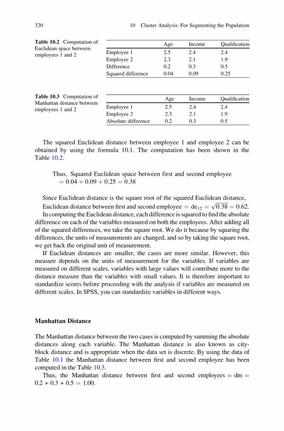
The squared Euclidean distance between employee 1 and employee 2 can be
obtained by using the formula 10.1. The computation has been shown in the
Table 10.2.
Thus; Squared Euclidean space between first and second employee
¼ 0:04þ 0:09þ 0:25 ¼ 0:38
Since Euclidean distance is the square root of the squared Euclidean distance,
Euclidean distance between first and second employee ¼ de12 ¼ffiffiffiffiffiffiffiffiffi0:38
p ¼ 0:62:In computing the Euclidean distance, each difference is squared to find the absolute
difference on each of the variables measured on both the employees. After adding all
of the squared differences, we take the square root. We do it because by squaring the
differences, the units of measurements are changed, and so by taking the square root,
we get back the original unit of measurement.
If Euclidean distances are smaller, the cases are more similar. However, this
measure depends on the units of measurement for the variables. If variables are
measured on different scales, variables with large values will contribute more to the
distance measure than the variables with small values. It is therefore important to
standardize scores before proceeding with the analysis if variables are measured on
different scales. In SPSS, you can standardize variables in different ways.
Manhattan Distance
TheManhattan distance between the two cases is computed by summing the absolute
distances along each variable. The Manhattan distance is also known as city-
block distance and is appropriate when the data set is discrete. By using the data of
Table 10.1 the Manhattan distance between first and second employee has been
computed in the Table 10.3.
Thus, the Manhattan distance between first and second employees ¼ dm ¼0.2 + 0.3 + 0.5 ¼ 1.00.
Table 10.3 Computation of
Manhattan distance between
employees 1 and 2
Age Income Qualification
Employee 1 2.5 2.4 2.4
Employee 2 2.3 2.1 1.9
Absolute difference 0.2 0.3 0.5
Table 10.2 Computation of
Euclidean space between
employees 1 and 2
Age Income Qualification
Employee 1 2.5 2.4 2.4
Employee 2 2.3 2.1 1.9
Difference 0.2 0.3 0.5
Squared difference 0.04 0.09 0.25
320 10 Cluster Analysis: For Segmenting the Population

Chebyshev Distance
The Chebyshev distance between the two cases are obtained by finding the
maximum absolute difference in values for any variable. This distance is computed
if we want to define two cases as “different” if they differ on any one of the
dimensions. The Chebyshev distance is computed as
Chebyshev distance x; yð Þ ¼ dc ¼ Max xi � yij j (10.2)
In Table 10.1, the Chebyshev distance between the first and fourth employees
would be 2.8 as this is the maximum absolute difference of these two employees on
income variable.
Mahalanobis (or Correlation) Distance
The Mahalanobis distance is based on the Pearson correlation coefficient which is
computed between the observations of two cases or subjects. This correlation
coefficient is used to cluster the cases. This is an important measure as it is a
scale invariant. In other words, it is not affected by the change in units of the
observations. Thus, the Mahalanobis distance (dm) between first and second
employees can be obtained by computing the correlation coefficient between the
observations 2.5, 2.4, 2.4 and 2.3, 2.1, 1.9.
Pearson Correlation Distance
The Pearson distance (dp) is also based on the Pearson correlation coefficient
between the observations of the two cases. This distance is computed as dp ¼ 1�rand lies between 0 and 2. Since the maximum and minimum values of r can be +1
and �1, respectively, the range of the Pearson distance (dp) can be from 0 to 2. The
zero value of dp indicates that the cases are alike, and 2 indicates that the cases are
entirely distinct.
Clustering Procedure
In cluster analysis, each case/object is considered to be a single cluster. The
distances between these objects are computed by the chosen distance measure.
On the basis of these distances computed in the proximity matrix, several objects
are linked together. After having done so, how do we determine the distances
between these new clusters? In other words, we need to have a linkage or amal-
gamation criteria to determine when two clusters are sufficiently similar to be
linked together. There are various protocols: for example, we may link two clusters
Terminologies Used in Cluster Analysis 321

together on the basis of the smallest distance between the two objects, one from
each of the two different clusters. Similarly the two clusters may be linked together
on the basis of the maximum distance between the two objects, one from each
cluster. There are different ways the objects can be clustered together. The entire
clustering procedures can be broadly classified in three different categories, that is,
hierarchical clustering, nonhierarchical clustering, and two-step clustering. These
procedures shall be discussed in detail under various headings in this section. The
details of various classification procedures have been shown graphically in
Fig. 10.1.
Hierarchical Clustering
In hierarchical clustering, objects are organized into a hierarchical structure.
It creates a hierarchy of clusters which may be represented in a treelike structure
known as dendrogram. Objects are grouped into a tree of clusters by using the
distance (similarity) matrix as clustering criteria. In this tree structure, the root
consists of a single cluster containing all observations, whereas the leaves refer to
the individual observations. Hierarchical clustering is the best for small data sets
because in this procedure a proximity matrix of the distance/similarity is computed
for each pair of cases in the data set.
Hierarchical clustering can be either agglomerative or divisive. In agglomerative
clustering, one starts at the individual objects and successively merges clusters
together. On the other hand, in the divisive clustering, one starts with all the objects
as one cluster and recursively splits the clusters. We shall now discuss various types
of clustering protocols of these two types of hierarchical clustering in detail.
Clustering Procedure
Hierarchical clustering
Agglomerative clustering Divisive clustering
Centroid methods
Variance methods
Linkage methods
Ward’s procedure
Single linkage Complete linkage Average linkage
Sequential Threshold method
Parallel Threshold method
Optimizing Partitioning method
Two-step clusterNon-Hierarchical clustering(K means clustering)
Fig. 10.1 Different clustering procedures
322 10 Cluster Analysis: For Segmenting the Population

Agglomerative Clustering
In agglomerative clustering, all the individual objects/cases are considered as a
separate cluster. These objects (atomic clusters) are successively merged into bigger
and bigger clusters using specified measure of similarity between the pair of objects.
The choice of which clusters to merge is determined by a linkage criteria. Thus, in
agglomerative clustering, we start at the leaves and successively clusters are merged
together to form the dendrogram. The clusters shall keepmergingwith each other until
all of the objects are in a single cluster or until certain termination conditions are
satisfied. The termination condition is decided by the researcher which depends upon
the number of clusters required to be formed. One of the criteria in deciding the
number of clusters to be formed depends upon whether some meanings can be
attached to these clusters or not. Consider the following raw data in Fig. 10.2. Each
data is a case/object and is considered to be the independent cluster. Depending upon
the distances, these clusters are merged in different steps, and finally we get a single
cluster. The formation of these clusters at different stages is shown in Fig. 10.3.
Fig. 10.2 Raw data showing
the distances between the
objects
Fig. 10.3 Formation of clusters at different stages in agglomerative clustering
Terminologies Used in Cluster Analysis 323

In agglomerative clustering, different methods are used to form the clusters.
These methods are discussed below.
Centroid Method
In this method, clusters are merged on the basis of the Euclidean distance between
the cluster centroids. Clusters having least Euclidean distance between their
centroids are merged together. In this method, if two unequal sized groups are
merged together, then larger of the two tends to dominate the merged cluster. Since
centroid methods compare the means of the two clusters, outliers affect it less than
most other hierarchical clustering methods. However, it may not perform well in
comparison to Ward’s method or average linkage method (Milligan 1980). Linkage
of clusters using centroid method is shown in Fig. 10.4.
Variance Methods
In this method, clusters are formed that minimize the within cluster variance. In other
words, clusters are linked if the variation within the two clusters is least. This is done
by checking the squared Euclidean distance to the center mean. The method used in
checking the minimum variance in forming clusters is known as Ward’s minimum
variance method. This method tends to join the clusters having small number of
observations and is biased towards producing clusters with same shape and with
nearly equal number of observations. The variance method is very sensitive to the
outliers. If “a” to “g” represents seven clusters then cluster formation using Ward’s
method can be shown graphically in Fig. 10.5.
Linkage Methods
In agglomerative clustering, clusters are formed on the basis of three different types
of linkage methods.
Fig. 10.4 Linkage of clusters using centroid method
324 10 Cluster Analysis: For Segmenting the Population

1. Single Linkage Method: In this method, clusters are formed on the basis of
minimum distance between the closest members of the two clusters. This is also
known as nearest neighbor rule. This kind of linkage can be seen in Fig. 10.6.
2. Complete Linkage Method: In this method, clusters are formed on the basis of
minimum distance between the farthest members of the two clusters. This is also
known as furthest neighbor rule. Complete linkage can be shown by Fig. 10.7.
3. Average Linkage Method: This procedure uses the minimum average distance
between all pairs of objects (in each pair one member must be from a different
cluster) as the criteria to make the next higher cluster. Average linkage can be
shown by Fig. 10.8.
Fig. 10.5 Linkage of clusters using variance method
Fig. 10.6 Clusters based on
single linkage
Fig. 10.7 Clusters based on
complete linkage
Fig. 10.8 Clusters based on
average linkage
Terminologies Used in Cluster Analysis 325

Divisive Clustering
In divisive clustering, we start by considering all individual objects/cases as one
cluster (called as root) and recursively splits into smaller and smaller clusters owing
to any of the distance criteria, until each object forms a cluster on its own or until it
satisfies certain termination conditions which depend upon the number of clusters
to be formed. Here, data objects are grouped in a top down fashion. Thus, in
divisive clustering, we start at the root and reaches to leaves. Divisive clustering
is just the reverse of agglomerative clustering. Cluster formation in divisive clus-
tering schedule can be seen in Fig. 10.9.
Nonhierarchical Clustering (K-Means Cluster)
Unlike hierarchical clustering, in K-means clustering, a number of clusters are
decided in advance. Solutions cannot be obtained for a range of clusters unless
you rerun the analysis every time for different number of clusters. In K-means
clustering, the first step is to find the K-centers. We start with an initial set of
K-means and classify cases/objects based on their distances to the centers. Next, the
cluster means are computed again using the cases/objects that are assigned to the
cluster. After this, we reclassify all cases/objects based on the new set of means.
This iterative process keeps going until cluster means do not change much between
successive steps. Once the stability of cluster means is achieved, the means of the
clusters are calculated once again and all the cases are assigned to their permanent
clusters. If one can have a good guesses for the initial K-centers, those can be used
as initial starting points; otherwise, let the SPSS find K cases that are well separated
and use these values as initial cluster centers.
In hierarchical clustering, distance or similarity matrix between all pair of cases is
required to be computed. This matrix becomes voluminous if the number of cases
Fig. 10.9 Formation of clusters at different stages in divisive clustering
326 10 Cluster Analysis: For Segmenting the Population

is in thousands. Because of this, so much processing is required, and even with the
modern computer, one needs to wait for some time to get the results. On the other hand,
k-means clustering method does not require computation of all possible distances.
Nonhierarchical clustering solution has three different approaches, that is, sequen-
tial threshold method, parallel threshold, and optimizing partitioning method.
The sequential threshold method is based on finding a cluster center and then
grouping all objects that are within a specified threshold distance from the center.
Here, one cluster is created at a time.
In parallel threshold method, several cluster centers are determined simulta-
neously and then objects are grouped depending upon the specified threshold
distance from these centers. These threshold distances may be adjusted to include
more or fewer objects in the clusters.
The optimizing partitioning is similar to other two nonhierarchical methods
except it allows for reassignment of objects to another cluster depending on some
optimizing criterion. In this method, a nonhierarchical procedure is run first, and
then objects are reassigned so as to optimize an overall criterion.
Precautions: K-means clustering is very sensitive toward the outliers because
they will usually be selected as initial cluster centers. If outlier exists in the data,
this will result in outliers forming clusters with small number of cases. Therefore, it
is important for the researcher to screen the data for outliers and remove them
before starting the cluster analysis.
Two-Step Cluster
Two-step clustering procedure is an exploratory statistical tools used for identifying
the natural grouping of cases/objects within a large data set. It is an efficient
clustering procedure in a situation where the data set is very large. This procedure
has an ability to create clusters if some of the variables are continuous and others
are categorical. It provides automatic identification of number of clusters present in
the data.
There are two assumptions in this analysis: first, the variables are independent,
and, second, each continuous variable follows a normal distribution whereas each
categorical variable has a multinomial distribution. The two-step cluster analysis
procedure provides solution in two steps which are explained as follows:
Step 1: Pre-cluster Formation
Pre-clusters are the clusters of original cases/objects that are used in place of raw
data to reduce the size of the distance matrix between all possible pair of cases.
After completing the pre-clustering, the cases in the same pre-cluster are treated as
a single entity. Thus, the size of the distance matrix depends upon the number of
pre-clusters instead of cases. Hierarchical clustering method is used on these pre-
clusters instead of the original cases.
Terminologies Used in Cluster Analysis 327

Step 2: Clustering Solutions Using Pre-clusters
In the second step, the standard hierarchical clustering algorithm is used on the pre-
clusters for obtaining the cluster solution. The agglomerative clustering algorithm
may be used to produce a range of cluster solutions. To determine which number of
clusters is the best, each of these cluster solutions may be compared using either
Schwarz’s Bayesian criterion (BIC) or the Akaike information criterion (AIC) as
the clustering criterion. The readers are advised to read about these procedures from
some other texts.
Standardizing the Variables
Cluster analysis is normally used for the data measured on interval scale and rarely
used for ratio data. In cluster analysis, distances are computed between the pair of
cases on each of the variables. And if the units of measurement for these variables
are different, then one must be worried about its impact on these distances.
Variables having larger values will have a larger impact on the distance com-
pared to variables that have smaller values. In that case, one must standardize the
variables to a mean of 0 and a standard deviation of 1.
If the variables are measured on interval scale and range of scale is same for each
of the variable, then standardization of variables is not required, but if its range of
measurement scale is different for different variables or if they are measured on
ratio scale, then one must standardize the variables in some way so that they all
contribute equally to the distance or similarity between cases.
Icicle Plots
It is the plotting of cases joining to form the clusters at each stage. You can see in
Fig. 10.10 what is happening at each step of the cluster analysis when average
linkage between groups is used to link the clusters. The figure is called an icicle plotbecause the columns representing cases look like icicles hanging from eaves. Each
column represents one of the case/object you are clustering. Each row represents a
cluster solution with different numbers of clusters.
If you look at the figure from bottom up, the last row (not shown) is the first step of
the analysis. Each of the cases is a cluster of its own. The number of clusters at that
point is 6. The five-cluster solution arises when the cases “a” and “b” are joined into a
cluster. It is so because they had the smallest distance of all pairs. The four-cluster
solution results from the merging of the cases “d” and “e” into a cluster. The three-
cluster solution is the result of combining the cases “c” with “de.” Going similarly,
for the one cluster solution, all of the cases are combined into a single cluster.
328 10 Cluster Analysis: For Segmenting the Population

Remarks
1. When pairs of cases are tied for the smallest distance to form a cluster, an arbitrary
selection is made. And, therefore, if cases are sorted differently, you might get a
different cluster solution. But that should not bother you as there is no right or
wrong answer to a cluster analysis. Many groupings are equally viable.
2. In case of large number of cases in cluster analysis, icicle plot can be developed
by taking cases as rows. You must specify the “Horizontal” on the Cluster Plots
dialog box.
The Dendrogram
The dendrogram is the graphical display of the distances on which clusters are com-
bined. The dendrogram can be seen in Fig. 10.22 and is read from left to right. Vertical
lines show joined clusters. The position of the line on the scale represents the distance at
which clusters are joined. The observed distances are rescaled to fall into the range of
1–25, and hence you do not see the actual distances; however, the ratio of the rescaled
distanceswithin the dendrogram is the same as the ratio of the original distances. In fact,
the dendrogram is the graphical representation of the information provided by the
agglomeration schedule.
The Proximity Matrix
Consider the data of four employees on three different parameters age, income, and
qualification as shown in the Table 10.4. Let us see how the proximity matrix is
developed on these data.
The proximity matrix is the arrangement of squared Euclidean distances in rows and
columns obtained between all pairs of cases. The squared Euclidean distances shall be
computed by adding the squared differences between the two employees on each of the
three variables.
a b c d e f
Number 1 X X X X X X X X X X X Xof 2 X X X X X X X X X X XClusters 3 X X X X X X X X X
4 X X X X X X X X5 X X X X X X X
Fig. 10.10 Vertical icicle plot
Terminologies Used in Cluster Analysis 329

The distance between employees 1 and 2 ¼ (2.5�2.3)2 + (2.4�2.1)2 +
(2.4�1.9)2 ¼ .04 + .09 + .25 ¼ 0.38
The distance between employees 1 and 4 ¼ (2.5–1.5)2 + (2.4 + 0.4)2 +
(2.4�1.3)2 ¼ 1.00 + 7.84 + 1.21 ¼ 10.05
The distance between employees 2 and 3 ¼ (2.3�1.2)2 + (2.1�1.9)2 +
(1.9 + 0.9)2 ¼ 1.21 + 0.04 + 1.00 ¼ 2.25
This way, all distances can be computed which are shown in Table 10.5. This
table is known as the proximity matrix.
All the entries in the diagonal are 0 because an employee does not differ with
himself. The smallest difference between two employees is 0.38, the distance
between the employee 1 and employee 2. The largest distance, 12.83, occurs
between employee 1 and employee 3. The distance matrix is symmetric, and,
therefore, you can see that the distance between the first and third employee is
same as the distance between the third and first employee.
What We Do in Cluster Analysis
In using cluster analysis, one needs to follow different steps to get the final results.
You may not understand all the steps at this moment but use it as a blueprint of the
analysis and proceed further, and I am sure by the time you finish reading the entire
chapter, you will have a fairly good idea about its application. Once you understand
different concepts of cluster analysis discussed in this chapter, you will be taken to a
solved example by using SPSS, and this will give you practical knowledge of using
this analysis to your data set with SPSS. Below are the steps which are used in
cluster analysis:
1. Identify the variables on which subjects/objects need to be clustered.
Table 10.4 Employees’
profileAge Income Qualification
Employee 1 2.5 2.4 2.4
Employee 2 2.3 2.1 1.9
Employee 3 1.2 1.9 �0.9
Employee 4 1.5 �0.4 1.3
Table 10.5 Proximity matrix
Squared Euclidean Distance
Cases Employee 1 Employee 2 Employee 3 Employee 4
Employee 1 0 0.38 12.83 10.05
Employee 2 0.38 0 2.25 7.25
Employee 3 12.83 2.25 0 10.22
Employee 4 10.05 7.25 10.22 0
330 10 Cluster Analysis: For Segmenting the Population
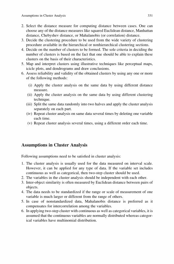
2. Select the distance measure for computing distance between cases. One can
choose any of the distance measures like squared Euclidean distance, Manhattan
distance, Chebyshev distance, or Mahalanobis (or correlation) distance.
3. Decide the clustering procedure to be used from the wide variety of clustering
procedure available in the hierarchical or nonhierarchical clustering sections.
4. Decide on the number of clusters to be formed. The sole criteria in deciding the
number of clusters is based on the fact that one should be able to explain these
clusters on the basis of their characteristics.
5. Map and interpret clusters using illustrative techniques like perceptual maps,
icicle plots, and dendrograms and draw conclusions.
6. Assess reliability and validity of the obtained clusters by using any one or more
of the following methods:
(i) Apply the cluster analysis on the same data by using different distance
measure.
(ii) Apply the cluster analysis on the same data by using different clustering
technique.
(iii) Split the same data randomly into two halves and apply the cluster analysis
separately on each part.
(iv) Repeat cluster analysis on same data several times by deleting one variable
each time.
(v) Repeat cluster analysis several times, using a different order each time.
Assumptions in Cluster Analysis
Following assumptions need to be satisfied in cluster analysis:
1. The cluster analysis is usually used for the data measured on interval scale.
However, it can be applied for any type of data. If the variable set includes
continuous as well as categorical, then two-step cluster should be used.
2. The variables in the cluster analysis should be independent with each other.
3. Inter-object similarity is often measured by Euclidean distance between pairs of
objects.
4. The data needs to be standardized if the range or scale of measurement of one
variable is much larger or different from the range of others.
5. In case of nonstandardized data, Mahalanobis distance is preferred as it
compensates for intercorrelation among the variables.
6. In applying two-step cluster with continuous as well as categorical variables, it is
assumed that the continuous variables are normally distributed whereas categor-
ical variables have multinomial distribution.
Assumptions in Cluster Analysis 331

Research Situations for Cluster Analysis Application
Cluster analysis can be applied to a wide variety of research problems in the area of
management, psychology, medicine, pharmaceuticals, social sciences, etc. Follow-
ing are the situations where this technique can be applied:
1. Cluster analysis can be used to classify the consumer population into market
segments for understanding the requirements of potential customers in different
groups. Such studies may be useful in segmenting the market, identifying the
target market, product positioning, and developing new products.
2. In a big departmental store, all inventories may be clustered into different groups
for placing them in same location or giving the similar code for enhancing sale
and easy monitoring of the products.
3. In the field of psychiatry, the cluster analysis may provide the cluster of
symptoms such as paranoia and schizophrenia, which is essential for successful
therapy.
4. In educational research, all schools of a district can be classified into different
clusters on the basis of the parameters like number of children, teacher’s
strength, total grant, school area, and location to develop and implement the
programs and policies effectively for each of these groups separately.
5. In the area of mass communication, television channels may be classified into
homogenous groups based on certain characteristics like TRP, number of
programs televised per week, number of artists engaged, coverage time,
programs in different sectors, advertisements received, and turnover. Different
policies may be developed for different groups of channels by the regulatory
body.
6. In medical research, cluster analysis may provide the solution for clustering of
diseases so that new drugs may be developed for different clusters of diseases.
This analysis may also be useful in clustering the patients on the basis of
symptoms for easy monitoring of drug therapy on mass scale.
Steps in Cluster Analysis
By learning terminologies involved in cluster analysis and the guidelines discussed
in the heading “What We Do in Cluster Analysis?”, you are now in a better position
to understand the procedure of its use for addressing your objectives. The cluster
analysis is usually done in two stages. The whole analysis is carried out in two
stages, the details of which have been discussed in the following steps:
Stage 1
1. The first step in cluster analysis is to apply the hierarchical cluster analysis in
SPSS to find the agglomerative schedule and proximity matrix for the data
obtained on each of the variables for all the cases. To form clusters, you need
332 10 Cluster Analysis: For Segmenting the Population
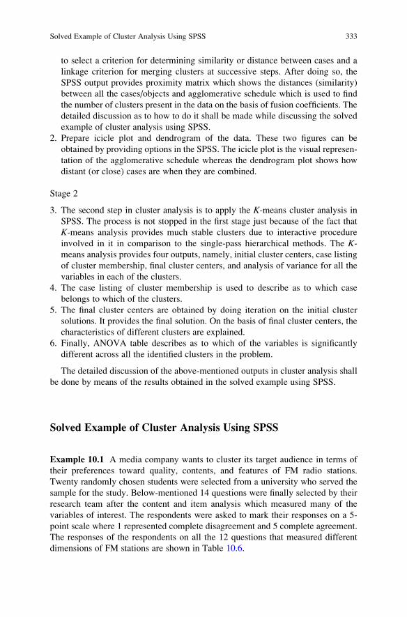
to select a criterion for determining similarity or distance between cases and a
linkage criterion for merging clusters at successive steps. After doing so, the
SPSS output provides proximity matrix which shows the distances (similarity)
between all the cases/objects and agglomerative schedule which is used to find
the number of clusters present in the data on the basis of fusion coefficients. The
detailed discussion as to how to do it shall be made while discussing the solved
example of cluster analysis using SPSS.
2. Prepare icicle plot and dendrogram of the data. These two figures can be
obtained by providing options in the SPSS. The icicle plot is the visual represen-
tation of the agglomerative schedule whereas the dendrogram plot shows how
distant (or close) cases are when they are combined.
Stage 2
3. The second step in cluster analysis is to apply the K-means cluster analysis in
SPSS. The process is not stopped in the first stage just because of the fact that
K-means analysis provides much stable clusters due to interactive procedure
involved in it in comparison to the single-pass hierarchical methods. The K-means analysis provides four outputs, namely, initial cluster centers, case listing
of cluster membership, final cluster centers, and analysis of variance for all the
variables in each of the clusters.
4. The case listing of cluster membership is used to describe as to which case
belongs to which of the clusters.
5. The final cluster centers are obtained by doing iteration on the initial cluster
solutions. It provides the final solution. On the basis of final cluster centers, the
characteristics of different clusters are explained.
6. Finally, ANOVA table describes as to which of the variables is significantly
different across all the identified clusters in the problem.
The detailed discussion of the above-mentioned outputs in cluster analysis shall
be done by means of the results obtained in the solved example using SPSS.
Solved Example of Cluster Analysis Using SPSS
Example 10.1 A media company wants to cluster its target audience in terms of
their preferences toward quality, contents, and features of FM radio stations.
Twenty randomly chosen students were selected from a university who served the
sample for the study. Below-mentioned 14 questions were finally selected by their
research team after the content and item analysis which measured many of the
variables of interest. The respondents were asked to mark their responses on a 5-
point scale where 1 represented complete disagreement and 5 complete agreement.
The responses of the respondents on all the 12 questions that measured different
dimensions of FM stations are shown in Table 10.6.
Solved Example of Cluster Analysis Using SPSS 333
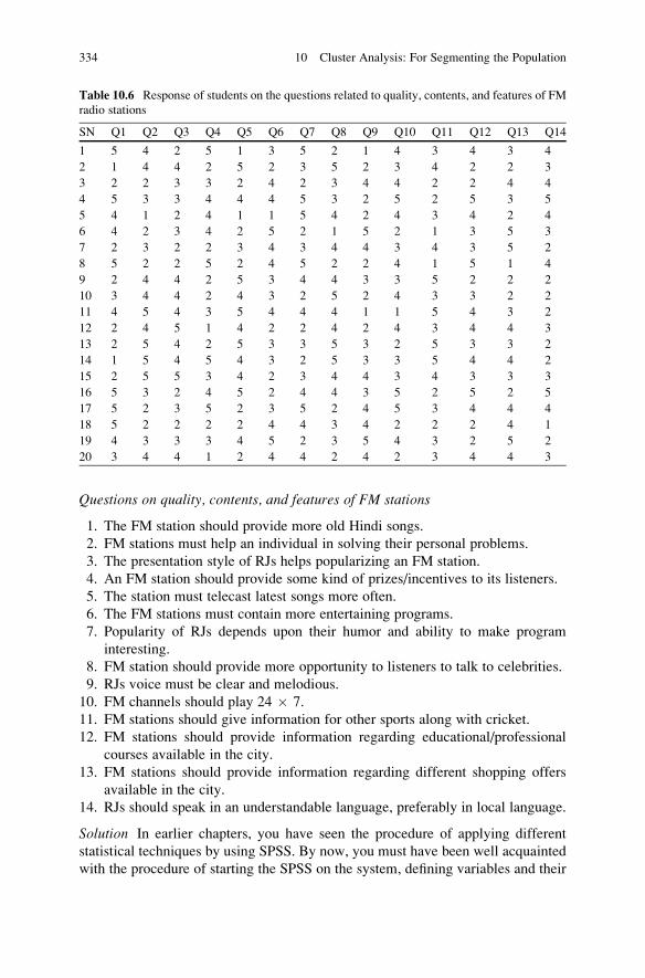
Questions on quality, contents, and features of FM stations
1. The FM station should provide more old Hindi songs.
2. FM stations must help an individual in solving their personal problems.
3. The presentation style of RJs helps popularizing an FM station.
4. An FM station should provide some kind of prizes/incentives to its listeners.
5. The station must telecast latest songs more often.
6. The FM stations must contain more entertaining programs.
7. Popularity of RJs depends upon their humor and ability to make program
interesting.
8. FM station should provide more opportunity to listeners to talk to celebrities.
9. RJs voice must be clear and melodious.
10. FM channels should play 24 � 7.
11. FM stations should give information for other sports along with cricket.
12. FM stations should provide information regarding educational/professional
courses available in the city.
13. FM stations should provide information regarding different shopping offers
available in the city.
14. RJs should speak in an understandable language, preferably in local language.
Solution In earlier chapters, you have seen the procedure of applying different
statistical techniques by using SPSS. By now, you must have been well acquainted
with the procedure of starting the SPSS on the system, defining variables and their
Table 10.6 Response of students on the questions related to quality, contents, and features of FM
radio stations
SN Q1 Q2 Q3 Q4 Q5 Q6 Q7 Q8 Q9 Q10 Q11 Q12 Q13 Q14
1 5 4 2 5 1 3 5 2 1 4 3 4 3 4
2 1 4 4 2 5 2 3 5 2 3 4 2 2 3
3 2 2 3 3 2 4 2 3 4 4 2 2 4 4
4 5 3 3 4 4 4 5 3 2 5 2 5 3 5
5 4 1 2 4 1 1 5 4 2 4 3 4 2 4
6 4 2 3 4 2 5 2 1 5 2 1 3 5 3
7 2 3 2 2 3 4 3 4 4 3 4 3 5 2
8 5 2 2 5 2 4 5 2 2 4 1 5 1 4
9 2 4 4 2 5 3 4 4 3 3 5 2 2 2
10 3 4 4 2 4 3 2 5 2 4 3 3 2 2
11 4 5 4 3 5 4 4 4 1 1 5 4 3 2
12 2 4 5 1 4 2 2 4 2 4 3 4 4 3
13 2 5 4 2 5 3 3 5 3 2 5 3 3 2
14 1 5 4 5 4 3 2 5 3 3 5 4 4 2
15 2 5 5 3 4 2 3 4 4 3 4 3 3 3
16 5 3 2 4 5 2 4 4 3 5 2 5 2 5
17 5 2 3 5 2 3 5 2 4 5 3 4 4 4
18 5 2 2 2 2 4 4 3 4 2 2 2 4 1
19 4 3 3 3 4 5 2 3 5 4 3 2 5 2
20 3 4 4 1 2 4 4 2 4 2 3 4 4 3
334 10 Cluster Analysis: For Segmenting the Population
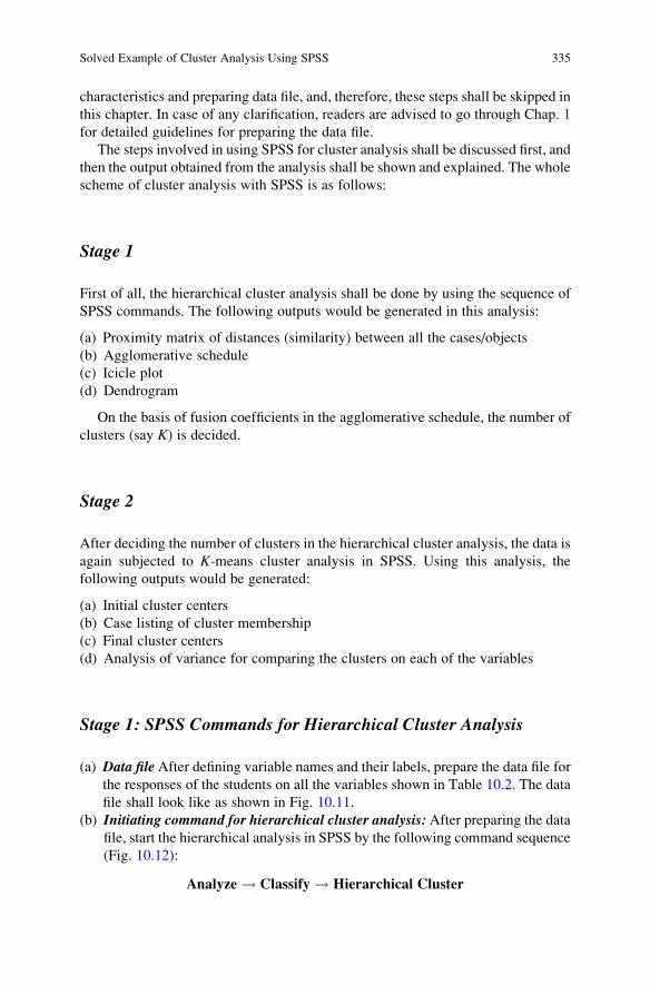
characteristics and preparing data file, and, therefore, these steps shall be skipped in
this chapter. In case of any clarification, readers are advised to go through Chap. 1
for detailed guidelines for preparing the data file.
The steps involved in using SPSS for cluster analysis shall be discussed first, and
then the output obtained from the analysis shall be shown and explained. The whole
scheme of cluster analysis with SPSS is as follows:
Stage 1
First of all, the hierarchical cluster analysis shall be done by using the sequence of
SPSS commands. The following outputs would be generated in this analysis:
(a) Proximity matrix of distances (similarity) between all the cases/objects
(b) Agglomerative schedule
(c) Icicle plot
(d) Dendrogram
On the basis of fusion coefficients in the agglomerative schedule, the number of
clusters (say K) is decided.
Stage 2
After deciding the number of clusters in the hierarchical cluster analysis, the data is
again subjected to K-means cluster analysis in SPSS. Using this analysis, the
following outputs would be generated:
(a) Initial cluster centers
(b) Case listing of cluster membership
(c) Final cluster centers
(d) Analysis of variance for comparing the clusters on each of the variables
Stage 1: SPSS Commands for Hierarchical Cluster Analysis
(a) Data file After defining variable names and their labels, prepare the data file for
the responses of the students on all the variables shown in Table 10.2. The data
file shall look like as shown in Fig. 10.11.
(b) Initiating command for hierarchical cluster analysis: After preparing the datafile, start the hierarchical analysis in SPSS by the following command sequence
(Fig. 10.12):
Analyze ! Classify ! Hierarchical Cluster
Solved Example of Cluster Analysis Using SPSS 335

Fig. 10.12 Sequence of SPSS commands for hierarchical cluster
Fig. 10.11 Showing data file for all the variables in SPSS
336 10 Cluster Analysis: For Segmenting the Population
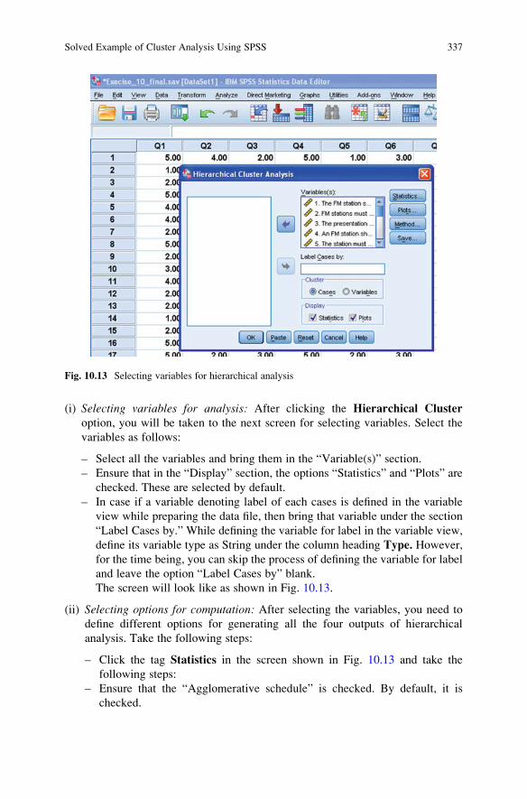
(i) Selecting variables for analysis: After clicking the Hierarchical Cluster
option, you will be taken to the next screen for selecting variables. Select the
variables as follows:
– Select all the variables and bring them in the “Variable(s)” section.
– Ensure that in the “Display” section, the options “Statistics” and “Plots” are
checked. These are selected by default.
– In case if a variable denoting label of each cases is defined in the variable
view while preparing the data file, then bring that variable under the section
“Label Cases by.” While defining the variable for label in the variable view,
define its variable type as String under the column heading Type. However,
for the time being, you can skip the process of defining the variable for label
and leave the option “Label Cases by” blank.
The screen will look like as shown in Fig. 10.13.
(ii) Selecting options for computation: After selecting the variables, you need to
define different options for generating all the four outputs of hierarchical
analysis. Take the following steps:
– Click the tag Statistics in the screen shown in Fig. 10.13 and take the
following steps:
– Ensure that the “Agglomerative schedule” is checked. By default, it is
checked.
Fig. 10.13 Selecting variables for hierarchical analysis
Solved Example of Cluster Analysis Using SPSS 337
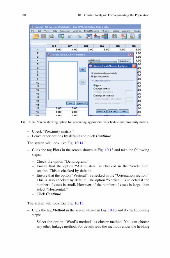
– Check “Proximity matrix.”
– Leave other options by default and click Continue.
The screen will look like Fig. 10.14.
– Click the tag Plots in the screen shown in Fig. 10.13 and take the following
steps:
– Check the option “Dendrogram.”
– Ensure that the option “All clusters” is checked in the “icicle plot”
section. This is checked by default.
– Ensure that the option “Vertical” is checked in the “Orientation section.”
This is also checked by default. The option “Vertical” is selected if the
number of cases is small. However, if the number of cases is large, then
select “Horizontal.”
– Click Continue.
The screen will look like Fig. 10.15.
– Click the tagMethod in the screen shown in Fig. 10.13 and do the following
steps:
– Select the option “Ward’s method” as cluster method. You can choose
any other linkage method. For details read the methods under the heading
Fig. 10.14 Screen showing option for generating agglomerative schedule and proximity matrix
338 10 Cluster Analysis: For Segmenting the Population

Distance Method discussed earlier. Personally I prefer the Ward’s
method as it depends upon the minimum variance concept and gives
the clusters which are more homogenous within itself.
– Select the option “Squared Euclidean distance” as an interval measure.
However, you can choose any other method as a distance measure like
Euclidean distance, Pearson correlation method, or Chebyshev method.
But generally squared Euclidean method is used to find the distance in the
proximity matrix.
– Select the option “None” in the “Transform Values” section. This is so
because in our example, the units of measurement for all the variables are
same. However, if the units of measurements are different, one needs to
standardize the variables. The most popular transformation is “Z-scores”
which needs to be selected if the measurement units are different for all
the variables.
– Check the option “Absolute values” in the “TransformMeasures” option.
This option transforms the values generated by the distance measure.
This option is not required for squared Euclidean distance.
Fig. 10.15 Selecting options for dendrogram and icicle plot
Solved Example of Cluster Analysis Using SPSS 339

– Click Continue. You will be taken back to the screen shown in Fig. 10.13.
The screen will look like as shown in Fig. 10.16.
– Click OK
(c) Getting the output: Clicking the option OK shall generate lot of outputs in the
output window. The four outputs that would be selected are Proximity matrix,
Agglomerative schedule, Icicle plot, and Dendrogram. These outputs have been
shown in Tables 10.7, 10.8 and Fig. 10.21, 10.22.
Stage 2: SPSS Commands for K-Means Cluster Analysis
Stage 1 was the explorative process where number of initial clusters was identified.
These initial clusters were identified on the basis of fusion coefficients in the
agglomerative schedule. After deciding the number of clusters, apply the K-means cluster analysis in stage 2. In stage 1, three clusters were identified on the
basis of the agglomeration schedule in Table 10.8 (for details, see Interpretation of
Findings). This shall be used to find the final solution in the K-means cluster
Fig. 10.16 Selecting options for cluster method and distance measure criteria
340 10 Cluster Analysis: For Segmenting the Population

analysis. The data file developed for the hierarchical analysis is also used for the
K-means cluster analysis. Follow these steps in stage 2.
(i) Initiating command for K-means cluster analysis: Start the K-means analysis by
using the following command sequence (Fig. 10.17):
Analyze ! Classify ! K-Means Cluster Analysis
(ii) Selecting variables for analysis: After clicking the K-Means Cluster Analysis
option, you will be taken to the next screen for selecting variables. Select the
variables as follows:
– Select all the variables and bring them in the “Variable(s)” section.
– Write number of clusters as 3. This is so because only three clusters were
identified from the hierarchical analysis.
– Click the option Iterate and ensure that the minimum iteration is written as
10. In fact, this is done by default. If you want to have more than 10
maximum iterations, it may be mentioned here.
– Click Continue.
Fig. 10.17 Sequence of SPSS commands for K-means cluster
Solved Example of Cluster Analysis Using SPSS 341
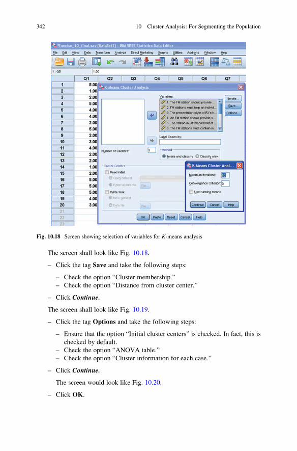
The screen shall look like Fig. 10.18.
– Click the tag Save and take the following steps:
– Check the option “Cluster membership.”
– Check the option “Distance from cluster center.”
– Click Continue.
The screen shall look like Fig. 10.19.
– Click the tag Options and take the following steps:
– Ensure that the option “Initial cluster centers” is checked. In fact, this is
checked by default.
– Check the option “ANOVA table.”
– Check the option “Cluster information for each case.”
– Click Continue.
The screen would look like Fig. 10.20.
– Click OK.
Fig. 10.18 Screen showing selection of variables for K-means analysis
342 10 Cluster Analysis: For Segmenting the Population

Fig. 10.19 Screen showing option for getting cluster memberships and distance from cluster
center
Fig. 10.20 Screen showing options for cluster information and ANOVA

Interpretations of Findings
Stage 1: The agglomerative cluster analysis done in stage 1 provided the outputs
shown in Tables 10.7 and 10.8 and in Figs. 10.21 and 10.22. The agglomerative
analysis is explorative in nature. Its primary purpose is to identify the initial cluster
solution. Therefore, one should take all possible parameters to identify the clusters
so that important parameters are not left out. We shall now discuss the results
generated in the agglomerative analysis in stage 1.
Proximity Matrix: To Know How Alike (or Different) the Cases Are
Table 10.7 is a proximity matrix which shows distances between the cases. One can
choose any distance criterion like squared Euclidean distance, Manhattan distance,
Chebyshev distance, Mahalanobis (or correlation) distance, or Pearson correlation
distance. In this example, the squared Euclidean distance was chosen as a measure
of distance. The minimum distance exists between the 9th and 13th cases which is
6.00, whereas the maximum distance is observed between the 8th and 13th cases
which is 87.00. The minimum distance means that these two cases would combine
at the very first instance. This can be seen from Table 10.8 where 9th and 13th cases
are combined into a single cluster in the very first stage. Similarly, the 8th and 13th
cases are in the extreme clusters which can be seen in the dendrogram shown in
Fig. 10.22.
Agglomerative Schedule: To Know How Should Clusters Be Combined
Table 10.8 is an agglomerative schedule which shows how and when the clusters
are combined. The agglomerative schedule is used to decide the number of clusters
present in the data and one should identify the number of clusters by using the
column labeled “Coefficients” in this table. These coefficients are also known as
fusion coefficients. The values under this column are the distance (or similarity)
statistic used to form the cluster. From these values, you get an idea as to how the
clusters have been combined. In case of using dissimilarity measures, small
coefficients indicate that those fairly homogenous clusters are being attached to
each other. On the other hand, large coefficients show that the dissimilar clusters are
being combined. In using similarity measures, the reverse is true, that is, large
coefficients indicate that the homogeneous clusters are being attached to each other,
whereas small coefficients reveal that dissimilar clusters are being combined.
The value of fusion coefficient depends on the clustering method and the
distance measure you choose. These coefficients help you decide how many
clusters you need to represent the data. The process of cluster formation is stopped
when the increase (for distance measures) or decrease (for similarity measures) in
344 10 Cluster Analysis: For Segmenting the Population

Table
10.7
Proxim
itymatrix
Case
Squared
Euclideandistance
12
34
56
78
910
11
12
13
14
15
16
17
18
19
20
1.000
68.000
45.000
19.000
21.000
52.000
52.000
16.000
61.000
51.000
49.000
60.000
69.000
62.000
54.000
33.000
17.000
45.000
58.000
42.000
268.000
.000
39.000
57.000
55.000
82.000
30.000
80.000
7.000
11.000
29.000
16.000
9.000
24.000
12.000
49.000
71.000
59.000
48.000
42.000
345.000
39.000
.000
40.000
40.000
19.000
17.000
47.000
40.000
30.000
64.000
31.000
46.000
43.000
31.000
46.000
30.000
28.000
17.000
25.000
419.000
57.000
40.000
.000
30.000
51.000
49.000
15.000
52.000
40.000
46.000
45.000
60.000
61.000
47.000
10.000
16.000
50.000
45.000
41.000
521.000
55.000
40.000
30.000
.000
65.000
49.000
23.000
56.000
46.000
66.000
55.000
68.000
67.000
53.000
28.000
22.000
44.000
67.000
51.000
652.000
82.000
19.000
51.000
65.000
.000
34.000
48.000
71.000
61.000
73.000
62.000
73.000
68.000
56.000
65.000
33.000
23.000
20.000
28.000
752.000
30.000
17.000
49.000
49.000
34.000
.000
66.000
23.000
25.000
37.000
26.000
21.000
26.000
24.000
53.000
41.000
21.000
14.000
18.000
816.000
80.000
47.000
15.000
23.000
48.000
66.000
.000
73.000
57.000
67.000
74.000
87.000
84.000
70.000
25.000
21.000
47.000
64.000
52.000
961.000
7.000
40.000
52.000
56.000
71.000
23.000
73.000
.000
14.000
20.000
23.000
6.000
25.000
11.000
50.000
58.000
44.000
35.000
31.000
10
51.000
11.000
30.000
40.000
46.000
61.000
25.000
57.000
14.000
.000
26.000
11.000
14.000
25.000
15.000
36.000
54.000
40.000
31.000
33.000
11
49.000
29.000
64.000
46.000
66.000
73.000
37.000
67.000
20.000
26.000
.000
35.000
14.000
29.000
27.000
54.000
64.000
50.000
49.000
35.000
12
60.000
16.000
31.000
45.000
55.000
62.000
26.000
74.000
23.000
11.000
35.000
.000
19.000
28.000
14.000
45.000
57.000
53.000
38.000
26.000
13
69.000
9.000
46.000
60.000
68.000
73.000
21.000
87.000
6.000
14.000
14.000
19.000
.000
15.000
9.000
56.000
70.000
50.000
37.000
31.000
14
62.000
24.000
43.000
61.000
67.000
68.000
26.000
84.000
25.000
25.000
29.000
28.000
15.000
.000
14.000
59.000
61.000
67.000
40.000
46.000
15
54.000
12.000
31.000
47.000
53.000
56.000
24.000
70.000
11.000
15.000
27.000
14.000
9.000
14.000
.000
43.000
47.000
49.000
32.000
24.000
16
33.000
49.000
46.000
10.000
28.000
65.000
53.000
25.000
50.000
36.000
54.000
45.000
56.000
59.000
43.000
.000
26.000
58.000
51.000
55.000
17
17.000
71.000
30.000
16.000
22.000
33.000
41.000
21.000
58.000
54.000
64.000
57.000
70.000
61.000
47.000
26.000
.000
36.000
35.000
37.000
18
45.000
59.000
28.000
50.000
44.000
23.000
21.000
47.000
44.000
40.000
50.000
53.000
50.000
67.000
49.000
58.000
36.000
.000
21.000
23.000
19
58.000
48.000
17.000
45.000
67.000
20.000
14.000
64.000
35.000
31.000
49.000
38.000
37.000
40.000
32.000
51.000
35.000
21.000
.000
28.000
20
42.000
42.000
25.000
41.000
51.000
28.000
18.000
52.000
31.000
33.000
35.000
26.000
31.000
46.000
24.000
55.000
37.000
23.000
28.000
.000
Thisisadissimilaritymatrix
Solved Example of Cluster Analysis Using SPSS 345

Table 10.8 Agglomeration schedule
Stage
Cluster combined
Coefficients
Stage cluster first appears
Cluster 1 Cluster 2 Cluster 1 Cluster 2 Next stage
1 9 13 3.000 0 0 2
2 2 9 7.333 0 1 5
3 4 16 12.333 0 0 17
4 10 12 17.833 0 0 12
5 2 15 24.000 2 0 12
6 7 19 31.000 0 0 8
7 1 8 39.000 0 0 9
8 3 7 48.000 0 6 15
9 1 17 58.000 7 0 11
10 18 20 69.500 0 0 13
11 1 5 81.500 9 0 17
12 2 10 94.333 5 4 14
13 6 18 107.500 0 10 15
14 2 14 121.667 12 0 16
15 3 6 137.000 8 13 18
16 2 11 153.750 14 0 18
17 1 4 172.417 11 3 19
18 2 3 261.524 16 15 19
19 1 2 389.800 17 18 0
Fig. 10.21 Vertical icicle plot using Ward’s linkage
346 10 Cluster Analysis: For Segmenting the Population

the coefficients between the two adjacent steps is large. In this example, the process
can be stopped at the three cluster solution, after stage 17. Let us see how it is done?
We should look for the coefficients from the last row upward because we want
the lowest possible number of clusters due to economy and its interpretability.
Stage 20 represents a one cluster solution where all the cases are combined into one
cluster, and, therefore, it is not shown in Table 10.8. The largest difference
(389.800–261.524) exists in the coefficients between stages 18 and 19, which
means we have to stop the process of cluster formation after stage 19; this would
result in only two-cluster solution. However, we may not be interested to represent
the data by two clusters only; therefore, we will look for the next larger difference
of (261.524–172.417) which is equal to 89.107 (between stage 18, the three-cluster
solution, and stage 17, the four-cluster solution). The next one after that is
(172.417–153.750), only 18.667, between stages 17 and 16. Thereafter, the differ-
ence keeps decreasing. So we decide to stop the cluster formation at stage 18 which
is a three-cluster solution.
Thus, in general, the strategy is to first identify the largest difference in the
coefficients and identify the stage of the lowest coefficient as the cluster solution.
However, it is up to the researcher to decide the number of clusters depending upon
its interpretability. You can see from the dendrogram shown in Fig. 10.22 that three
clusters are clearly visible in this case.
Fig. 10.22 Dendrogram using Ward linkage
Solved Example of Cluster Analysis Using SPSS 347

The agglomeration schedule starts off using the case numbers that has smallest
distance as shown by the icicle plot in Fig. 10.21. The cluster is formed by adding
cases. The number of the lowest case becomes the number of this newly formed
cluster. For example, if a cluster is formed by merging cases 3 and 6, it would be
known as cluster 3, and if the clusters are formed by merging cases 3 and 1, then it
would be known as cluster 1.
The columns labeled “Stage Cluster First Appears” shows the step at which each
of the two clusters that are being joined first appear. For example, at stage 9 when
clusters 1 and 17 are combined, it tells you that cluster 1 was first formed at stage 7
and cluster 17 is a single case, and that the resulting cluster (known as 1) will see
action again at stage 11 (under the column “Next stage”). If number of cases are
small then the icicle plot explains step-by-step clustering summary better than the
agglomeration schedule.
The Icicle Plot: Summarizing the Steps
Figure 10.21 is the icicle plot which is a graphical representation of agglomerative
schedule. It tells you how the clusters are formed at each stage. The figure is called
an icicle plot because the columns look like icicles hanging from eaves. Each
column represents one of the objects you are clustering. Each row shows a cluster
solution with different number of clusters. You see the figure from the bottom up.
The last row (not shown) is the first step of the analysis. Each of the cases is a
cluster of itself. The number of clusters at this point is 20. The nineteen-cluster
solution arises when cases 9 and 13 are joined into a cluster. It happened because
they had the smallest distance among all pairs. The eighteen-cluster solution results
from the merging of case 2 with cluster 9 into a cluster. This will go on till all the
clusters are combined into a single cluster.
Remark: In case of large number of cases, icicle plot can be developed by
showing cases as rows. For this, specify Horizontal in the Cluster Plots dialog
box in SPSS.
The Dendrogram: Plotting Cluster Distances
Figure 10.22 shows the dendrogram which is used to show the plotting of cluster
distances. It provides a visual representation of the distance at which clusters are
combined. We read the dendrogram from left to right. A vertical line represents the
joined clusters. The position of the line on the scale shows the distance at which
clusters are joined. The computed distances are rescaled in the range of 1–25, and,
therefore, actual distances cannot be seen here; however, the ratio of the rescaled
distances within the dendrogram is the same as the ratio of the original distances.
The first vertical line, corresponding to the smallest rescaled distance, is for the
case 9 and case 13. The next vertical line is at the next smallest distance for the
cluster 9 and case 2. It can be seen from Table 10.8 that the lowest coefficient is
348 10 Cluster Analysis: For Segmenting the Population

3.000, which is for cases 9 and 13. The next smallest distance is shown by the
coefficient as 7.333 which is for cluster 9 and case 2. Thus, what you see in this plot
is what you already know from the agglomeration schedule.
Remark: While reading the dendrogram, one should try to determine at what stage
the distances between clusters that are combined is large. You look for large
distances between sequential vertical lines. In this case, large distance between
the vertical lines suggests a three-cluster solution.
Stage 2 With the help of hierarchical cluster analysis, the number of cluster was
decided to be three. After this, K-means cluster analysis was applied to get the final
solution of the cluster means. The SPSS generated the outputs in the form of
Tables 10.9, 10.10, 10.11, 10.12, 10.13, and 10.14. We shall now explain these
outputs and discuss the cluster characteristics.
Table 10.9 Initial cluster centers
Variables
Cluster
1 2 3
1. The FM station should provide more old Hindi songs 5.00 2.00 4.00
2. FM stations must help an individual in solving their personal problems 3.00 5.00 2.00
3. The presentation style of RJs helps popularizing an FM station 2.00 4.00 3.00
4. An FM station should provide some kind of prizes/incentives to its
listeners
4.00 2.00 4.00
5. The station must telecast latest songs more often 5.00 5.00 2.00
6. The FM stations must contain more entertaining programs 2.00 3.00 5.00
7. Popularity of RJs depends upon their humor and ability to make program
interesting
4.00 3.00 2.00
8. FM station should provide more opportunity to listeners to talk to
celebrities
4.00 5.00 1.00
9. RJs’ voice must be clear and melodious 3.00 3.00 5.00
10. FM channels should play 24 � 7 5.00 2.00 2.00
11. FM stations should give information for other sports along with cricket 2.00 5.00 1.00
12. FM stations should provide information regarding educational/professional
courses available in the city
5.00 3.00 3.00
13. FM stations should provide information regarding different shopping
offers available in the city
2.00 3.00 5.00
14. RJs should speak in an understandable language, preferably in local
language
5.00 2.00 3.00
Table 10.10 Iteration historya
Iteration Change in cluster centers
1 2 3
1 3.375 1.753 2.953
2 .000 .480 .566
3 .000 .000 .000aConvergence achieved due to no or small change in cluster centers. The maximum absolute
coordinate change for any center is .000. The current iteration is 3. The minimum distance between
initial centers is 7.483
Solved Example of Cluster Analysis Using SPSS 349
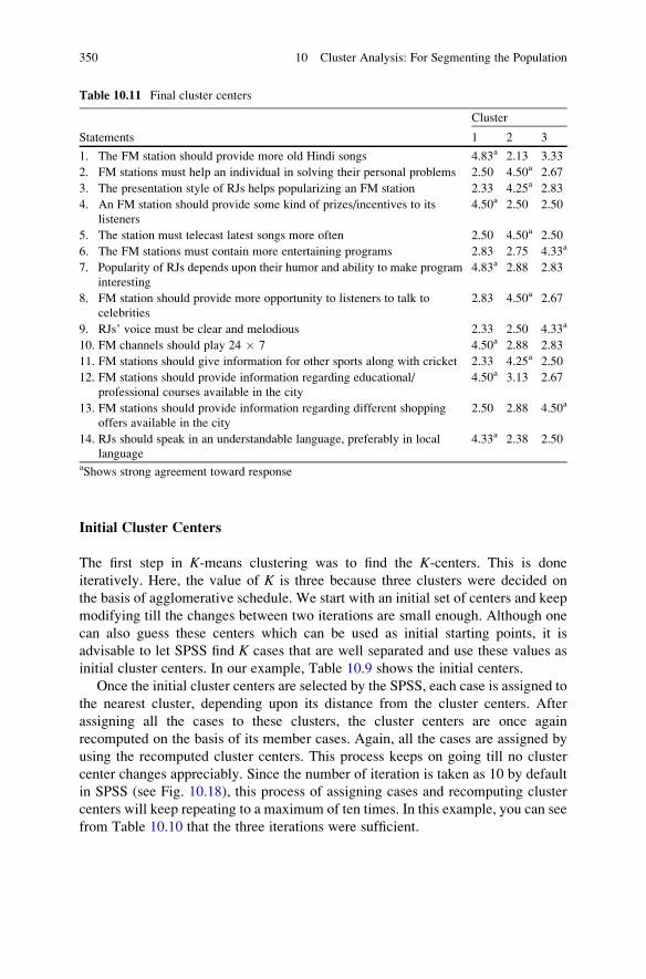
Initial Cluster Centers
The first step in K-means clustering was to find the K-centers. This is done
iteratively. Here, the value of K is three because three clusters were decided on
the basis of agglomerative schedule. We start with an initial set of centers and keep
modifying till the changes between two iterations are small enough. Although one
can also guess these centers which can be used as initial starting points, it is
advisable to let SPSS find K cases that are well separated and use these values as
initial cluster centers. In our example, Table 10.9 shows the initial centers.
Once the initial cluster centers are selected by the SPSS, each case is assigned to
the nearest cluster, depending upon its distance from the cluster centers. After
assigning all the cases to these clusters, the cluster centers are once again
recomputed on the basis of its member cases. Again, all the cases are assigned by
using the recomputed cluster centers. This process keeps on going till no cluster
center changes appreciably. Since the number of iteration is taken as 10 by default
in SPSS (see Fig. 10.18), this process of assigning cases and recomputing cluster
centers will keep repeating to a maximum of ten times. In this example, you can see
from Table 10.10 that the three iterations were sufficient.
Table 10.11 Final cluster centers
Statements
Cluster
1 2 3
1. The FM station should provide more old Hindi songs 4.83a 2.13 3.33
2. FM stations must help an individual in solving their personal problems 2.50 4.50a 2.67
3. The presentation style of RJs helps popularizing an FM station 2.33 4.25a 2.83
4. An FM station should provide some kind of prizes/incentives to its
listeners
4.50a 2.50 2.50
5. The station must telecast latest songs more often 2.50 4.50a 2.50
6. The FM stations must contain more entertaining programs 2.83 2.75 4.33a
7. Popularity of RJs depends upon their humor and ability to make program
interesting
4.83a 2.88 2.83
8. FM station should provide more opportunity to listeners to talk to
celebrities
2.83 4.50a 2.67
9. RJs’ voice must be clear and melodious 2.33 2.50 4.33a
10. FM channels should play 24 � 7 4.50a 2.88 2.83
11. FM stations should give information for other sports along with cricket 2.33 4.25a 2.50
12. FM stations should provide information regarding educational/
professional courses available in the city
4.50a 3.13 2.67
13. FM stations should provide information regarding different shopping
offers available in the city
2.50 2.88 4.50a
14. RJs should speak in an understandable language, preferably in local
language
4.33a 2.38 2.50
aShows strong agreement toward response
350 10 Cluster Analysis: For Segmenting the Population

Final Cluster Centers
Table 10.11 shows the final cluster centers after iteration stops, and cases are
reassigned to the clusters. Using these final cluster centers, cluster characteristic
are described.
Each question in this example is responded on a 1–5 scoring scale, where 5
stands for total agreement and 1 stands for total disagreement. Thus, if any score
shown in Table 10.11 is more than 2.5, it indicates the agreement toward the
statement, and if it is less than 2.5, it reflects disagreement. Thus, owing to these
Table 10.12 ANOVA table
Cluster Error
FSig. p-value
Mean
square df
Mean
square df
1. The FM station should provide more old Hindi
songs
12.579 2 .885 17 14.217 .000
2. FM stations must help an individual in solving
their personal problems
8.858 2 .637 17 13.901 .000
3. The presentation style of RJs helps popularizing
an FM station
7.042 2 .333 17 21.125 .000
4. An FM station should provide some kind of prizes/
incentives to its listeners
8.400 2 1.000 17 8.400 .003
5. The station must telecast latest songs more often 9.600 2 1.118 17 8.589 .003
6. The FM stations must contain more entertaining
programs
5.042 2 .686 17 7.346 .005
7. Popularity of RJs depends upon their humor
and ability to make program interesting
8.204 2 .620 17 13.230 .000
8. FM station should provide more opportunity to
listeners to talk to celebrities
7.392 2 .716 17 10.328 .001
9. RJs’ voice must be clear and melodious 7.667 2 .745 17 10.289 .001
10. FM channels should play 24 � 7 5.671 2 .777 17 7.299 .005
11. FM stations should give information for other
sports along with cricket
8.108 2 .843 17 9.617 .002
12. FM stations should provide information regarding
educational/professional courses available in the
city
5.546 2 .571 17 9.711 .002
13. FM stations should provide information regarding
different shopping offers available in the city
6.938 2 .699 17 9.932 .001
14. RJs should speak in an understandable language,
preferably in local language
7.646 2 .512 17 14.926 .000
The F-tests should be used only for descriptive purposes because the clusters have been chosen to
maximize the differences among cases in different clusters. The observed significance levels are
not corrected for this and thus cannot be interpreted as tests of the hypothesis that the cluster means
are equal
Solved Example of Cluster Analysis Using SPSS 351

criteria, the characteristics of these three clusters of cases were as follows (refer to
the question details in Example 10.1):
Cluster 1
FM listeners belonging to this cluster were of the strong opinion that channels
should provide more old Hindi songs (Q.1) and provide some incentives to the
listeners (Q.4). They strongly feel that the humor and ability to deliver interesting
programs make RJs more popular (Q.7). The channel should play 24 � 7 (Q.10)
and must air information regarding educational opportunity available in the city
(Q.12), and the RJ must speak in local dialect (Q.14).
Further, listeners belonging to this cluster feel that FM channels should air more
entertaining programs (Q.6) and should provide more opportunity to listeners to
talk to the celebrities (Q.8).
Table 10.13 Cluster
membershipCase number Cluster Distance
1 1 2.953
2 2 2.378
3 3 2.887
4 1 2.461
5 1 3.424
6 3 3.367
7 3 2.828
8 1 2.779
9 2 2.325
10 2 2.580
11 2 3.828
12 2 3.226
13 2 1.705
14 2 3.487
15 2 2.215
16 1 3.375
17 1 2.838
18 3 3.162
19 3 2.708
20 3 3.317
Table 10.14 Number of
cases in each clusterCluster 1 6.000
2 8.000
3 6.000
Valid 20.000
Missing .000
352 10 Cluster Analysis: For Segmenting the Population

Cluster 2
Listeners belonging to this cluster strongly felt that FM channels must provide
solutions to personal problems (Q.2), RJs presentation skill to be important for the
channels (Q.3), channels to provide more often the latest songs (Q.5), channels to
arrange more dialogues between celebrities and their audience (Q.8), and should air
information about sports other than cricket also (Q.11).
Further, listeners to this cluster also felt that FM channels should air more
entertaining programs (Q.6). Humor and ability to deliver interesting programs
make RJs more popular (Q.7). The channels must play 24 � 7 (Q.10) and should
provide information regarding educational opportunity (Q.12) and shopping offers
(Q.13) available in the city.
Cluster 3
Listeners in this cluster were strongly of the view that the FM channels must contain
more entertaining programs (Q.6), RJs voice must be very clear and melodious
(Q.9), and channels should provide information regarding shopping offers available
in the city (Q.13).
Further, listeners in this cluster were also of the view that channels should air
more old Hindi songs (Q.1), provide solution to the personal problems (Q.2), and
believe RJs to be the key factor in popularizing the FM channels (Q.3). They were
of the view that the humorous RJs make programs more interesting (Q.7). Channels
should provide more opportunity to listeners to talk to the celebrities (Q.8), they
should operate 24 � 7 (Q.10) and, at the same time, must air the information
regarding educational opportunities available in the city (Q.12).
ANOVA: To Know Differences Between Clusters
Table 10.12 shows ANOVA for the data on all the 14 variables. The F-ratioscomputed in the table describe the differences between the clusters. F-ratio is
significant at 5% level if the significance level (p-value) associated with it is less
than .05. Thus, it can be seen in Table 10.12 that F-ratios for all the variables are
significant at 5% level as their corresponding p-values are less than .05.
Remark
1. There is a divided opinion on the issue of using ANOVA analysis for comparing
the clusters on each of the parameters. The footnote in Table 10.12 warns that the
observed significance levels should not be interpreted in the usual fashion
because the clusters have been selected to maximize the differences between
clusters.
Solved Example of Cluster Analysis Using SPSS 353

2. It is up to the researcher to decide about using ANOVA for determining the
significance of variables. If ANOVA is used, then the interpretation of clusters
should be made on the basis of those variables which are significantly different
across clusters at any predefined level of significance.
Cluster Membership
Table 10.13 shows the cluster membership of the cases. You can see that six cases
belong to cluster 1, eight cases to cluster 2, and six cases to cluster 3.
Table 10.14 is a summary of Table 10.13. You do not like to see clusters with
very few cases unless they are really different from the remaining cases.
Exercise
Short Answer Questions
Q.1. Discuss a research situation where cluster analysis can be applied.
Q.2. Write the steps involved in cluster analysis.
Q.3. What is squared Euclidean distance? What impact it will have if the variables
are measured on different units? Suggest the procedure in that situation.
Q.4. When should you use Chebyshev distance and Mahalanobis distance? How
these distances are computed?
Q.5. How hierarchical clustering is different than K-means clustering?
Q.6. What is the difference between single linkage and average linkage method?
Q.7. What do you mean by Ward’s minimum variance method?
Q.8. What is the difference between agglomerative and divisive clustering? Can
both these clustering be shown in a single graph? If yes, how?
Q.9. In what situation two-stage clustering is done? Explain the steps in brief.
Q.10. Why hierarchical clustering is known as explorative technique? Explain
briefly the advantage of using this method.
Q.11. In cluster analysis, when do we need to standardize the variable and why?
Q.12. What do you mean by icicle plot and what it conveys? Show it by sketch.
Q.13. What is the purpose of proximity matrix? Develop a proximity matrix by
using any set of data on three cases measured on four variables.
Q.14. Discuss the assumptions used in cluster analysis.
Q.15. How the properties of clusters are explained?
Q.16. Would you agree to use ANOVA in cluster analysis? If yes, how clusters
should be explained, and, if not, why?
Q.17. In using SPSS for K-means cluster analysis, what output would be generated
if the option “Cluster interaction for each case” is chosen?
354 10 Cluster Analysis: For Segmenting the Population

Multiple-Choice Questions
Note: For each of the question, there are four alternative answers. Tick mark the
one that you consider the closest to the correct answer.
Answer Q.1 to Q.4 on the basis of the following information. In a cluster
analysis, if the data on two cases are as follows:
Case 1 14 8 10
Case 2 10 11 12
1. The squared Euclidean distance shall be
(a) 27
(b) 29
(c) 28
(d)ffiffiffiffiffi29
p
2. The Manhattan distance shall be
(a) 81
(b) 9
(c) 3
(d)ffiffiffi9
p
3. The Chebyshev distance shall be
(a) 4
(b) 3
(c) 2
(d) 9
4. The Euclidean distance shall be
(a) 29
(b) 30
(c)ffiffiffiffiffi29
p(d) 28
5. Cluster analysis is a(n)
(a) Explorative analysis
(b) Descriptive analysis
(c) Deductive analysis
(d) Predictive analysis
Exercise 355

6. When cluster is formed in agglomerative clustering by joining case 3 with
case 7, then the resultant cluster would be known as
(a) Cluster 7
(b) Cluster 3
(c) Cluster 3,7
(d) Cluster 7,3
7. In Ward’s method, any two clusters are joined to form a new cluster if
(a) The variation within each cluster is same
(b) The variation within one cluster is minimum than other
(c) The variation within the two clusters is least
(d) The variation between both the clusters is maximum
8. In complete linkage method, the clusters are formed on the basis of
(a) Minimum distance between the closest members of the two clusters
(b) Minimum average distance between all pairs of objects (in each pair, one
member must be from a different cluster)
(c) Minimum square Euclidean distances between any two clusters
(d) Minimum distance between the farthest members of the two clusters
9. The number of clusters is decided on the basis of fusion coefficients in
agglomerative schedule. In doing so, if distance matrix is considered, then
(a) We look for the largest difference in the coefficients
(b) We look for the smallest difference in the coefficients
(c) We look for the equality of the coefficients
(d) It is up to the researcher to decide any criteria
10. In cluster analysis, the characteristics of the clusters are decided on the basis of
(a) Initial cluster solution
(b) Final cluster solution
(c) Cluster membership
(d) ANOVA table
Assignments
1. The data on five nutritional contents of different food articles are shown in
Table-A. Identify the suitable clusters of food articles based on these five
nutritional contents. Use centroid clustering method and squared Euclidean
distances to find the clusters. Apply hierarchical clustering and then K-means
clustering method to find the final solution for clusters. Explain your findings
and discuss the characteristics of different clusters.
2. Ratings were obtained on different brands of car for their six parameters shown
in the Table-B. These cars are in specific prize range. The rating 1 indicates
complete agreement and 5 indicates complete disagreement. Apply cluster
analysis to discuss the characteristics of identified clusters of cars. Use Ward’s
method of clustering and squared Euclidean distance measure for cluster forma-
tion. Use the label cases option in SPSS.
356 10 Cluster Analysis: For Segmenting the Population
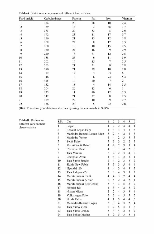
Table-B Ratings on
different cars on their
characteristics
S.N. Car 1 2 3 4 5 6
1 Logan 4 2 2 4 4 4
2 Renault Logan Edge 4 3 3 4 3 3
3 Mahindra-Renault Logan Edge 3 2 4 2 4 3
4 Mahindra Verito 4 4 2 3 3 3
5 Swift Dzire 3 3 3 2 2 3
6 Maruti Swift Dzire 4 2 2 3 3 4
7 Chevrolet Beat 4 3 1 4 2 5
8 Tata Venture 5 2 2 3 4 2
9 Chevrolet Aveo 4 3 3 2 3 1
10 Tata Sumo Spacio 2 4 2 3 3 2
11 Skoda New Fabia 3 5 3 5 4 4
12 Hyundai i10 4 4 3 4 3 3
13 Tata Indigo e-CS 3 3 4 3 3 2
14 Maruti Suzuki Swift 4 4 3 2 4 4
15 Maruti Suzuki A-Star 2 5 2 4 2 1
16 Maruti Suzuki Ritz Genus 3 4 3 5 5 2
17 Premier Rio 1 3 4 2 3 2
18 Nissan Micra 2 2 4 3 3 4
19 Volkswagen Polo 3 3 4 5 5 5
20 Skoda Fabia 4 1 5 4 4 5
21 Mahindra-Renault Logan 3 3 4 3 2 4
22 Tata Sumo Victa 2 2 5 3 3 3
23 Tata Sumo Grande 3 4 4 2 2 2
24 Tata Indigo Marina 4 2 5 3 3 1
Table-A Nutritional components of different food articles
Food article Carbohydrates Protein Fat Iron Vitamin
1 354 20 28 10 2.4
2 89 13 3 38 1.7
3 375 20 33 8 2.6
4 192 23 11 17 3.7
5 116 21 13 12 1.8
6 169 24 8 12 1.5
7 160 18 10 115 2.5
8 320 24 16 9 2.9
9 220 8 31 12 2.5
10 158 25 6 11 5.9
11 202 19 15 7 2.5
12 263 21 21 9 2.8
13 280 21 29 10 2.8
14 72 12 3 83 6
15 46 8 6 74 5.4
16 415 14 40 7 2
17 132 18 4 14 3.5
18 204 20 12 6 1
19 125 11 40 12 2.3
20 342 21 27 8 2.5
21 189 22 10 9 2.7
22 136 23 5 22 2.8
(Hint: Transform your data into Z-scores by using the commands in SPSS)

Parameters of the Car
1. The leg space in the car is comfortable.
2. Car space is big enough to keep my luggage during outing.
3. The car is giving the same mileage as mentioned in the brochure.
4. Driving is very comfortable.
5. Security feature of the car is good.
6. Accessories provided in the car are of good quality.
Besides explaining the characteristics of clusters, also answer the following:
(a) What are the minimum and maximum distances between the cases?
(b) How many clusters you would like to identify and what is the maximum
distance between the fusion coefficients?
(c) What criteria you would adopt to discuss the properties of the clusters?
(d) Explain cluster characteristics on the basis of ANOVA and see if it is different
than what you have explained earlier.
(e) How many cases/cars are in each cluster?
Answers to Multiple-Choice Questions
Q.1 b Q.2 b Q.3 a Q.4 c
Q.5 a Q.6 b Q.7 c Q.8 d
Q.9 a Q.10 b
358 10 Cluster Analysis: For Segmenting the Population

Chapter 11
Application of Factor Analysis: To Study
the Factor Structure Among Variables
Learning Objectives
After completing this chapter, you should be able to do the following:
• Understand the factor analysis and its application.
• Learn the difference between exploratory and confirmatory factor analysis.
• Know the use of factor analysis in developing test batteries.
• Interpret different terms involved in factor analysis.
• Explain the situations where factor analysis can be used.
• Know the procedure of retaining the factors and identifying the variables in it.
• Explain the steps involved in factor analysis.
• Understand the steps involved in using SPSS for factor analysis.
• Discuss the outputs obtained in factor analysis.
• Learn to write the results of factor analysis in standard format.
Introduction
Buying decision of an individual depends upon large number of product
characteristics. But the market strategy cannot be developed on the basis of all
those parameters of a product that affect the buying behavior of an individual. The
factor analysis, a multivariate technique, comes to our rescue in solving such
problems. The factor analysis technique reduces the large number of variables
into few underlying factors to explain the variability of the group characteristics.
The concept used in factor analysis technique is to investigate the relationship
among the group of variables and segregate them in different factors on the basis of
their relationship. Thus, each factor consists of those variables which are related
among themselves and explain some portion of the group variability. For example,
personality characteristics of an individual can be assessed by the large number of
parameters. The factor analysis may group these variables into different factors
J.P. Verma, Data Analysis in Management with SPSS Software,DOI 10.1007/978-81-322-0786-3_11, # Springer India 2013
359
where each factor measure some dimension of personality characteristics. Factors
are so formed that the variables included in it are related with each other in some
way. The significant factors are extracted to explain the maximum variability of the
group under study.
In marketing research, application of factor analysis provides very useful inputs
to the decision makers to focus on few factors rather than a large number of
parameters in making their products more acceptable in the market. For instance,
consider an automobile company is interested to know as to what makes their
customer to choose a particular model of the car. Several issues like mileage, easy
loan facility, roof height, leg space, maintenance, road clearance, steering function-
ality, brakes, lighting, and luggage space may be investigated by taking the
responses from the consumers. There may be endless issues on which the opinion
of the customers can be taken. But by using the factor analysis, these variables may
be clubbed in different factors like economy (mileage, easy loan facility), comfort(roof height, leg space, maintenance, luggage space), and technology (steering
functionality, brakes, lighting, and road clearance). Thus, instead of concentrating
on so many parameters, the authorities will make a strategy to optimize these three
factors for the growth of their business. Further, these factors may be used to
construct the perceptual maps and other product positioning.
Thus, in factor analysis, few factors are extracted out of the large set of variables.
Since variables in each of the factors are associated among themselves, therefore
they represent the same phenomenon. In this way, instead of studying all the
parameters, few extracted factors are studied. These factors so extracted explain
much of the variations of the group characteristics.
Factor analysis is used for both exploratory as well as confirmatory studies.
In exploratory study, we do not know anything about the number of factors to be
extracted, the number of variables included in each factor and percentage of variability
explained by these extracted factors. The researcher takes all those variables under
study which are suggested by the review studies or guided by the researchers own
knowledge or experts opinion. Exploratory studies are just like mining important
variables from a large number of variables to form factors. Unimportant variables do
not figure in any of the identified factors. Such variables are excluded on the basis of
their low communality. The process will be discussed later in the book. Thus, through
exploratory study, a researcher can extract the factors underlying all prospective
variables which have been selected on the pretext that they explain some or other
dimension of the group behavior. Such study also reveals the number of variables
which loads on each factor significantly and the percentage variability explained by
each factor toward the group characteristics.
On the other hand in confirmative factor analysis, it is required to test the
existing factor model. In other words, before starting the experiments, it is assumed
that the factor analysis will produce only specified number of factors and specific
number of variables are loaded on each factor and that the how much variability
shall be explained by the identified factors. Thus, a factor model developed in an
exploratory study is being tested in the confirmatory study to have its validity.
The factor analysis can be used to develop test battery for assessing group
characteristics. To assess employee’s performance, several variables like timeliness,
360 11 Application of Factor Analysis: To Study the Factor Structure Among Variables

cost-effectiveness, absenteeism, tardiness, creativity, quality, adherence to policy,
gossip and other personal habits, personal appearance, manager’s appraisal, self-
appraisal, and peer appraisal are usually measured. By using factor analysis, these
variables can be clubbed into different factors. On the basis of variable’s loading and
their explainability, one or two variables from each factor can be selected to form the
test battery. However, to validate the test battery, the confirmatory factor analysis
must be done on similar but different sample groups.
Another application of factor analysis is in developing of a questionnaire. While
doing item analysis, unimportant questions are removed from the questionnaire.
Factor analysis may be used to indicate the loss in the measurement of variability in
removing the unimportant questions from the final questionnaire. Further, it helps
in classifying the questions into different parameters in the questionnaire.
What Is Factor Analysis?
Factor analysis is a multivariate statistical technique used to identify the factors
underlying the variables by means of clubbing related variables in the same factor.
It is a dimension reduction technique which reduces the large number of variables
into few factors without sacrificing much, the power of explained variability by the
variables. Variables are clubbed into different factors on the basis of their interre-
lation. In initial solution of factor analysis, variables may belong to more than one
factor. But by using the factor rotation technique, these factors may be made
mutually exclusive. Thus, instead of defining the group characteristics by the
large number of variables, a few factors may do this job. The number of factors is
identified by means of the criterion known as eigenvalue. The magnitude of
variable’s loading on the factor is used as a criterion for retaining that variable in
the factor. Sufficient number of data set is required to run the factor analysis. As a
thumb rule, number of data set should be at least five per variable. Thus, if there are
15 variables in the problem, the sample must be approximately 75. However, there
is a procedure of testing the adequacy of sample size in running the factor analysis.
This is done by using the KMO test. We shall discuss it in detail later in this chapter.
Terminologies Used in Factor Analysis
To understand the factor analysis technique, it is essential to know the meaning of
various terms involved in it. It is assumed that the readers are familiar with the basic
logic of statistical reasoning and the concepts of variance and correlation; if not, it is
advised that they should read the basic statistics topic at this point, from the earlier
chapters discussed in this book.
Terminologies Used in Factor Analysis 361

Principal Component Analysis
Principal component analysis (PCA) is closely related to factor analysis. It is used
to reduce the large number of variables into smaller number of principal
components that will account for most of the variance in the observed variables.
In this method, the factor explaining the maximum variance is extracted first.
Principal component analysis method is used when the data on large number of
variables are obtained and some of the variables are redundant. Here, redundancy
means that some of the variables are correlated with one another, possibly because
they are measuring the same construct. Because of this redundancy, one believes
that it should be possible to reduce the observed variables into a smaller number of
principal components that will account for most of the variance in the observed
variables. In fact, principal component analysis is similar to the procedure used in
exploratory factor analysis
One must understand that the principal component analysis and factor analysis
are not same. In PCA, one performs a variance-maximizing rotation of the variable
space, and it takes into account all variability in the variables. On the other hand,
factor analysis is the procedure of estimating the amount of variability explained
due to common factors (communality). These two methods become same if the
error terms in the factor analysis model (the variability not explained by common
factors) can be assumed to have the same variance.
Factor Loading
Factor loading can be defined as the correlation coefficient between the variable and
factor. Just like Pearson’s r, the squared factor loading of a variable indicates the
percentage variability explained by the factor in that variable. As a rule of thumb,
0.7 or higher factor loading represents that the factor extracts sufficient variance
from that variable. The percentage variance explained in all the variables accounted
for by each factor can be computed by dividing the sum of the squared factor
loadings for that factor divided by the number of variables and multiplied by 100.
Communality
The communality can be defined as the sum of the squared factor loadings of a
variable in all the factors. It is the variance in that variable accounted for by all the
factors. The communality of variable is represented by h2. It measures the percent-
age of variance in a given variable explained by all the factors jointly and may be
considered as the reliability of the variable. Low communality of a variable
indicates that the variable is not useful in explaining the characteristics of the
362 11 Application of Factor Analysis: To Study the Factor Structure Among Variables

group and the factor model is not working well for that variable. Thus, variables
whose communalities are low should be removed from the model as such variables
are not related to each other. Any variable whose communality is <.4 should
usually be dropped. However, the communalities must be interpreted in relation
to the interpretability of the factors. For instance a communality of .80 may seem to
be high but becomes meaningless, unless the factor on which the variable is loaded
is interpretable, normally it usually will be. On the other hand a communality of .25
may look to be low but becomes meaningful if the variable can well define the
factor.
Hence, it is not the value of communality of a variable that is important, but the
variable’s role in interpretation of the factor is the important consideration. How-
ever, the variable whose communality is very high usually explain the factor well.
If the value of communality is more than 1, then one must expect that something is
wrong with the solution. Such situation indicates that either sample is too small or
the researcher has identified too many or too few factors.
Eigenvalue
The eigenvalue for a given factor measures the variance in all the variables which is
accounted for by that factor. It is also called as characteristics root. The sum of the
eigenvalues of all the factors is equal to the number of variables. The decision about
the number of factors to be retained in the factor analysis is taken on the basis of
eigenvalues. If a factor has a low eigenvalue, then it is contributing little to the
explanation of variances in the variables and may be dropped. Eigenvalues measure
the amount of variation in the total sample accounted for by each factor.
Kaiser Criteria
While applying the factor analysis one needs to decide as to how many factors
should be retained. As per the Kaiser’s criteria only those factors having eigenvalue
>1 should be retained in the factor analysis. Initially each variable is supposed to
have its eigenvalue 1. Thus, it may be said that unless a factor extracts at least as
much as the equivalent of one original variable, it is dropped. This criterion was
proposed by Kaiser and is the most widely used by the researchers.
The Scree Plot
The scree plot is a graphical representation of the factors plotted along X-axis
against their eigenvalues, on the Y-axis. As one moves toward the X-axis (factors),
the eigenvalues drop. When the drop ceases and the curve makes an elbow toward
Terminologies Used in Factor Analysis 363

less steep decline, Cattell’s scree test says to drop all further components after the
one starting the elbow. Thus, the factors above the elbow in the plot are retained.
The scree test was developed by Cattell. “Scree” is a term used in geology. The
scree is the rubble at the bottom of a cliff. In scree test, if a factor is important, it will
have a large variance. The scree plot may look like Fig. 11.1.
Varimax Rotation
Unrotated factor solution obtained after applying the principal component analysis
is rotated by using any of the rotational technique to enhance the interpretability of
factors. The varimax rotation is the most widely used rotation technique in factor
analysis. It is an orthogonal rotation of the factor axes to maximize the variance of
the squared loadings of a factor on all the variables in a factor matrix, which has the
effect of relocating the original variables into extracted factor. After varimax
rotation, each factor will tend to have either large or small loadings of any particular
variable and thus facilitates a researcher to identify each variable in one and only
one factor. This is the most common rotation option. Other rotational strategies are
quartimax, equamax, direct oblimin, and promax methods which are not much used
by the researcher.
Scree plot
Component number
Eig
en v
alue
2 3 4 5 6 7 8 9 101
0
1
2
3
4
5
Fig. 11.1 Scree plot for the factors
364 11 Application of Factor Analysis: To Study the Factor Structure Among Variables

What Do We Do in Factor Analysis?
The factor analysis involves different steps which are discussed below. You may
not understand all the steps at a glance but do not lose heart and continue to read.
After reading these steps, once you go through the solved example discussed later in
this chapter, a full clarity of the concepts can be achieved. The steps discussed
below cannot be done manually but may be achieved by using any statistical
package. So try and relate these steps with the output of factor analysis.
1. Compute descriptive statistics for all the variables. Usually mean and standard
deviation are provided by the standard statistical packages while running the
factor analysis. However, you may run descriptive statistics program to compute
other descriptive statistics like skewness, kurtosis, standard error, and coefficient
of variability to understand the nature of the variables under study.
2. Prepare correlation matrix with all the variables taken in the study.
3. Apply KMO test to check the adequacy of data for running factor analysis. The
value of KMO ranges from 0 to 1. The larger the value of KMOmore adequate is
the sample for running factor analysis. As a convention, any value of KMOmore
than .5 signifies the adequacy of sample for running the factor analysis. A value
of 0 indicates that the distinct factors cannot be made and hence, the sample is
not adequate. On the other hand, if its value is approaching 1, then the factor
analysis yields distinct and reliable factors. Kaiser recommends accepting values
>0.5 as acceptable (values below this should lead you to either collect more data
or rethink which variables to include). Further, the values between 0.5 and 0.7
are mediocre, values between 0.7 and 0.8 are good, values between 0.8 and 0.9
are great, and values above 0.9 are superb (Hutcheson and Sofroniou 1999).
4. Apply Bartlett’s test of sphericity for testing the hypothesis that the correlation
matrix is not an identity matrix. If the correlation matrix is an identity matrix, the
factor analysis becomes inappropriate. Thus, if the Bartlett’s test of sphericity is
significant, it is concluded that the correlation matrix is not an identity matrix
and the factor analysis can be run.
5. Obtain unrotated factor solution by using principal component analysis. This will
provide you the number of factors along with their eigenvalues. We retain only
those factors whose along with their eigenvalues. This can also be shown
graphically by scree plot. This solution also provides the factor loadings of the
variables on different factors, percentage variability explained by each factor, and
the total variability explained by all the factors retained in the model.
6. Thus, this primary factor analysis solution can tell you the percentage of
variability explained by all the identified factors together. However, it is not
possible to identify the variables included in each factor because some of the
variables may belong to more than one factor. This problem is sorted out by
choosing the appropriate rotation technique.
What Do We Do in Factor Analysis? 365

7. Obtain final solution by using the varimax rotation option, available in SPSS.
Thiswill solve the problemof redundancy of variables in different factors. As a rule
of thumb, if the factor loading of any variable on a factor is equal or more than 0.7,
then it should belong to that factor. The reason for choosing 0.7 factor loading as a
cut off point is that because factor loading represents correlation coefficient hence
at least 49% (= 0.72) variability of the variable must be explained by the factor to
which it belongs. However, other variables whose loadings are <0.7 can also be
identified in that factor on the basis of its explainability.
8. Identified factors in step 6 are given names depending upon the nature of
variables included in it.
9. If the purpose of the factor analysis is to develop a test battery also, then one or
two variables from each factor may be selected on the basis of their magnitude
of loadings. These variables so selected may form the test battery. Each
variable in the test battery is assigned weight. The weights assigned to the
variable in the test battery depend upon the percentage variability explained by
the factor from which it belongs. Usually, the first factor explains the maxi-
mum variance, and therefore two or three variables may be kept from it
depending upon the nature of the variables and its explainability. From rest
of the factors, normally one variable per factor is selected, as the sole purpose
of the factor analysis is to reduce the number of variables so that the maximum
variance in the group may be explained.
Assumptions in Factor Analysis
While using the factor analysis, the following assumptions are made:
1. All the constructs which measure the concepts have been included in the study.
2. Sufficient sample size has been taken for factor analysis. Normally sample size
must be equal to 5–20 times the number of variables taken in the study.
3. No outlier is present in the data.
4. Multicollinearity among the variables does not exist.
5. Homoscedasticity does not exist between the variables because factor analysis is
a linear function of measured variables. The meaning of homoscedasticity
between the variables is that the variance around the regression line is the
same for all values of the predictor variable (X).
6. Variables should be linear in nature. Nonlinear variables may also be used after
transforming it into linear variables.
7. Data used in the factor analysis is based on interval scale or ratio scale.
366 11 Application of Factor Analysis: To Study the Factor Structure Among Variables

Characteristics of Factor Analysis
Following are some of the important features of factor analysis:
• The variables used in the factor analysis may be objective or subjective provided
subjective variables can be expressed into scores.
• The factor analysis extracts the hidden dimensions among the variables which
may not be observable from direct analysis.
• This analysis is simple and inexpensive to perform.
Limitations of Factor Analysis
Although the factor analysis is very useful multivariate statistical technique, how-
ever, it has some limitations as well.
• Much of the advantage of factor analysis technique can be achieved only if the
researcher is able to collect a sufficient set of product attributes. If some of the
important attributes are missed out, the results of factor analysis will not be
efficient.
• If majority of the variables are highly related to each other and distinct from
other items, factor analysis will assign a single factor to them. This will not
reveal other factors that capture more interesting relationships.
• Naming the factors may require researcher’s knowledge about the subject matter
and theoretical concepts, because often multiple attributes can be highly
correlated for no apparent reason.
Research Situations for Factor Analysis
Since factor analysis is used to study the group characteristics by means of
identified factors out of the large number of variables, it has tremendous application
in management, social sciences, and humanities. Few research applications are
discussed below:
1. To understand the buying behavior of a particular product, several parameters
like customer’s age, education, job status, salary, exposure to product advertise-
ment, and availability are responsible. Factor analysis may help the market
analysts to identify few factors instead of large number of parameters to develop
the marketing strategy for launching the product.
2. In a mall, it is interesting to see the buying behaviour of the customers. On the
basis of the customer’s purchase history, the articles may be clubbed together
and kept in nearby counters to enhance the sale.
Research Situations for Factor Analysis 367

3. In an educational institution, the administration may be interested to know the
factors that are responsible for enhancing the status of the institution. Such
accomplishment can be achieved by controlling a large number of parameters.
The factor analysis may extract the underlying factors like academic curriculum,
student’s facilities, counseling procedure, and placement opportunity on which
the administration may concentrate to improve its image instead of large number
of parameters.
4. To evaluate a product, a survey technique can be used to identify various
parameters. Based on it, factor analysis can identify few factors on which
management can take decisions to promote their product.
5. Factor analysis may be used to create a lifestyle questionnaire for evaluating the
quality of life. After dropping the questions from the questionnaire on the basis
of item analysis, factor analysis provides the insight as to how much efficiency
has been sacrificed due to it.
Solved Example of Factor Analysis Using SPSS
Example 11.1
An industrial researcher wanted to investigate the climate of an organization. A set
of 12 questions were developed to measure different parameters of the climate. The
subject could respond these questions on five-point scale with 5 indicating strongly
agree and 1 strongly disagree attitude towards the question. The responses obtained
on the questionnaire are shown in Table 11.1 along with the description of the
questions. Apply factor analysis technique to study the factor structure and suggest
the test battery that can be used for assessing the climate of any industrial organi-
zation. Also apply the scree test for retaining factors graphically and KMO test for
testing the adequacy of data.
Statements
1. Employees are encouraged to attend training programs organized by outside
agencies.
2. Any employee can reach up to the top level management position during their
carrier.
3. Employees are praised by the immediate boss for doing something useful in the
organization
4. Medical facilities for the employees and their families are excellent
5. Employees are given preference in jobs announced by the group of companies.
6. For doing some creative work or working creatively, employees get incentives
7. Employee’s children are honored for their excellent performance in their
education.
8. Employees are cooperative in helping each other to solve their professional
problems
9. Fees of employees children are reimbursed during their schooling
368 11 Application of Factor Analysis: To Study the Factor Structure Among Variables

10. Employees get fast promotion if their work is efficient and consistence
11. Senior managers are sensitive to the personal problems of their employees.
12. Employees get cheaper loan for buying vehicles.
SolutionBy applying the factor analysis following issues shall be resolved:
1. To decide the number of factors to be retained and the total variance explained
by these factors
2. To identify the variables in each factor retained in the final solution, on the basis
of its factor loadings
3. To give names to each factor retained on the basis of the nature of variables
included in it
4. To suggest the test battery for assessing the climate of any industrial
organization
5. To test the adequacy of sample size used in factor analysis
Table 11.1 Data on the
parameters of organizational
climate
S.N S1 S2 S3 S4 S5 S6 S7 S8 S9 S10 S11 S12
1 3 2 4 1 3 5 4 2 2 4 3 4
2 3 3 5 2 3 4 5 1 3 5 4 5
3 5 3 4 2 2 5 5 2 3 4 3 4
4 3 4 4 1 3 4 4 1 2 5 3 4
5 4 3 4 2 2 5 4 2 3 4 2 4
6 3 2 5 2 3 4 5 1 4 5 5 5
7 5 3 4 2 2 4 4 2 3 4 2 4
8 4 4 5 1 1 4 4 1 2 4 3 2
9 5 3 4 2 3 4 4 3 3 3 2 4
10 5 3 5 2 2 5 5 2 4 4 4 5
11 4 4 4 1 3 5 5 2 3 4 3 3
12 4 2 5 2 4 5 4 1 2 5 2 2
13 3 2 4 1 3 4 4 1 3 2 3 3
14 5 3 5 2 2 5 4 2 3 5 2 4
15 4 3 4 1 3 4 5 1 2 4 3 4
16 4 2 4 3 2 4 5 2 3 3 2 5
17 2 3 4 2 3 4 4 2 4 4 3 3
18 4 2 5 2 4 5 4 3 3 5 2 4
19 3 3 4 1 3 3 4 2 2 4 3 4
20 4 3 4 2 2 4 5 3 3 3 2 5
21 5 4 4 1 3 4 5 2 2 4 3 3
22 4 3 5 2 4 5 4 1 3 5 4 4
23 3 2 4 1 3 5 4 2 2 5 3 5
24 4 3 4 2 2 4 4 1 3 4 2 4
25 5 2 5 3 3 5 5 2 4 5 3 3
Solved Example of Factor Analysis Using SPSS 369

These objectives will be achieved by generating the output of factor analysis in
SPSS. Thus, the procedure of using SPSS for factor analysis in the given example
shall be discussed first, and thereafter the output shall be explained in the light of
the objectives to be fulfilled in this study.
SPSS Commands for the Factor Analysis
Before running the SPSS commands for factor analysis, a data file needs to be
prepared. By now, you must have been familiar in preparing the data file. If not, you
may go through the procedure discussed in Chap. 1 in this regard. Do the following
steps for generating outputs in factor analysis:
(i) Data file: In this problem, all 12 statements are independent variables. These
variables have been defined as ‘Scale’ variable because they were measured on
interval scale. Variables measured on interval as well as ratio scales are treated
as scale variable in SPSS. After preparing the data file by defining variable
names and their labels, it will look like Fig. 11.2.
(ii) Initiating command for factor analysis: Once the data file is prepared, click thefollowing command sequence in the Data View:
Fig. 11.2 Screen showing data file for the factor analysis in SPSS
370 11 Application of Factor Analysis: To Study the Factor Structure Among Variables
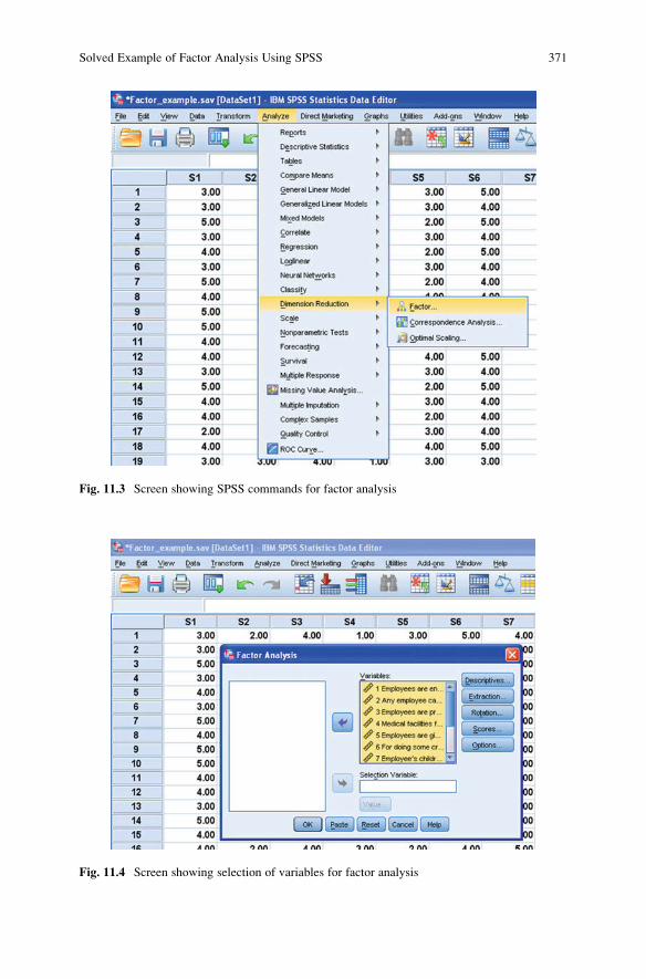
Fig. 11.3 Screen showing SPSS commands for factor analysis
Fig. 11.4 Screen showing selection of variables for factor analysis
Solved Example of Factor Analysis Using SPSS 371
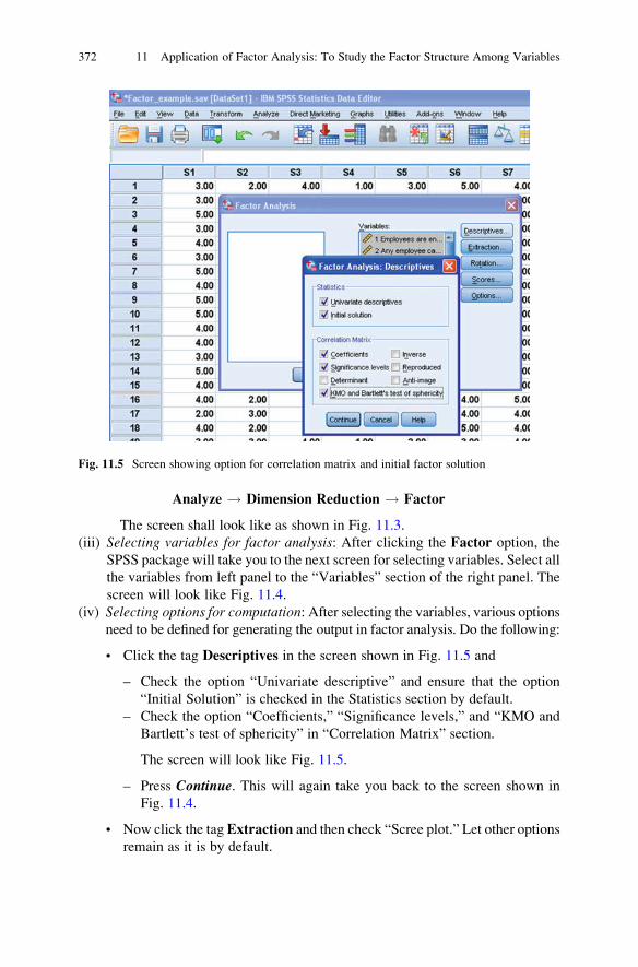
Analyze ! Dimension Reduction ! Factor
The screen shall look like as shown in Fig. 11.3.
(iii) Selecting variables for factor analysis: After clicking the Factor option, the
SPSS package will take you to the next screen for selecting variables. Select all
the variables from left panel to the “Variables” section of the right panel. The
screen will look like Fig. 11.4.
(iv) Selecting options for computation: After selecting the variables, various optionsneed to be defined for generating the output in factor analysis. Do the following:
• Click the tag Descriptives in the screen shown in Fig. 11.5 and
– Check the option “Univariate descriptive” and ensure that the option
“Initial Solution” is checked in the Statistics section by default.
– Check the option “Coefficients,” “Significance levels,” and “KMO and
Bartlett’s test of sphericity” in “Correlation Matrix” section.
The screen will look like Fig. 11.5.
– Press Continue. This will again take you back to the screen shown in
Fig. 11.4.
• Now click the tag Extraction and then check “Scree plot.” Let other options
remain as it is by default.
Fig. 11.5 Screen showing option for correlation matrix and initial factor solution
372 11 Application of Factor Analysis: To Study the Factor Structure Among Variables

Fig. 11.6 Screen showing option for unrotated factor solution and scree plot
Fig. 11.7 Screen showing option for factor rotation

The screen shall look like Fig. 11.6.
• Press Continue. This will again take you back to the screen shown in
Fig. 11.4.
• Now click the tag Rotation and then check “Varimax” rotation option. Let
other options remain as it is by default.
– The screen shall look like Fig. 11.7.
– Press Continue to go back to the main screen.
• Press OK for output.
(v) Getting the output: After pressing OK in the screen shown in Fig. 11.4, the
SPSS will generate the outputs in the output window. These outputs can be
selected by using the right click of the mouse and may be pasted in the word
file. The SPSS shall generate many outputs, but the following relevant outputs
have been selected for the discussion:
(a) Descriptive statistics
(b) Correlation matrix
(c) KMO and Bartlett’s test
(d) Communalities of all the variables
(e) Total variance explained
(f) Scree plot
(g) Component matrix: unrotated factor solution
(h) Rotated component matrix: varimax-rotated solution
In this example, all the outputs so generated by the SPSS are shown in
Tables 11.2–11.7 and Fig. 11.8.
Interpretation of Various Outputs Generated in Factor Analysis
The above-mentioned outputs generated in this example by the SPSS shall be
discussed to provide the answers to various issues related to model developed in
this study.
1. Table 11.2 shows the mean and SD for all the variables in the study. You may
add some more statistics like coefficient of variation, skewness, kurtosis, and
range to study the nature of variables. However, in that case, you have to use the
SPSS option of Descriptive discussed in Chap. 2 of this book.
2. Table 11.3 is the correlation matrix of all the variables. This is the first step in
factor analysis on the basis of which variables are grouped into factors. The
SPSS provides significance value (p value) for each correlation coefficient.
However, values of correlation coefficient required for its significance at 1%
as well as 5% can be seen from Table A.3 in the Appendix. Meaningful
conclusions can be drawn from this table for understanding relationships
among variables.
374 11 Application of Factor Analysis: To Study the Factor Structure Among Variables
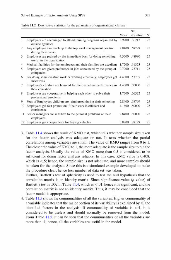
3. Table 11.4 shows the result of KMO test, which tells whether sample size taken
for the factor analysis was adequate or not. It tests whether the partial
correlations among variables are small. The value of KMO ranges from 0 to 1.
The closer the value of KMO to 1, the more adequate is the sample size to run the
factor analysis. Usually the value of KMO more than 0.5 is considered to be
sufficient for doing factor analysis reliably. In this case, KMO value is 0.408,
which is <.5; hence, the sample size is not adequate, and more samples should
be taken for the analysis. Since this is a simulated example developed to make
the procedure clear, hence less number of data set was taken.
Further, Bartlett’s test of sphericity is used to test the null hypothesis that the
correlation matrix is an identity matrix. Since significance value (p value) of
Bartlett’s test is .002 in Table 11.4, which is<.01, hence it is significant, and the
correlation matrix is not an identity matrix. Thus, it may be concluded that the
factor model is appropriate.
4. Table 11.5 shows the communalities of all the variables. Higher communality of
a variable indicates that the major portion of its variability is explained by all the
identified factors in the analysis. If communality of variable is <.4, it is
considered to be useless and should normally be removed from the model.
From Table 11.5, it can be seen that the communalities of all the variables are
more than .4; hence, all the variables are useful in the model.
Table 11.2 Descriptive statistics for the parameters of organizational climate
Mean
Std.
deviation N
1 Employees are encouraged to attend training programs organized by
outside agencies
3.9200 .86217 25
2 Any employee can reach up to the top level management position
during their carrier
2.8400 .68799 25
3 Employees are praised by the immediate boss for doing something
useful in the organization
4.3600 .48990 25
4 Medical facilities for the employees and their families are excellent 1.7200 .61373 25
5 Employees are given preference in jobs announced by the group of
companies
2.7200 .73711 25
6 For doing some creative work or working creatively, employees get
incentives
4.4000 .57735 25
7 Employee’s children are honored for their excellent performance in
their education
4.4000 .50000 25
8 Employees are cooperative in helping each other to solve their
professional problems
1.7600 .66332 25
9 Fees of Employees children are reimbursed during their schooling 2.8400 .68799 25
10 Employees get fast promotion if their work is efficient and
consistence
4.1600 .80000 25
11 Senior managers are sensitive to the personal problems of their
employees
2.8400 .80000 25
12 Employees get cheaper loan for buying vehicles 3.8800 .88129 25
Solved Example of Factor Analysis Using SPSS 375

Table
11.3
Correlationmatrixfortheparam
etersoftheorganizational
clim
ate
S1
S2
S3
S4
S5
S6
S7
S8
S9
S10
S11
S12
S1
10.188
0.17
0.35
�0.299
0.318
0.271
0.329
0.118
�0.041
�0.321
�0.068
S2
0.188
1�0
.193
�0.407*
�0.339
�0.252
0.073
�0.088
�0.232
�0.027
0.027
�0.239
S3
0.17
�0.193
10.349
0.175
0.354
0.068
�0.236
0.302
0.591**
0.366
�0.089
S4
0.35
�0.407*
0.349
1�0
.088
0.212
0.244
0.237
0.679**
0.095
�0.18
0.243
S5
�0.299
�0.339
0.175
�0.088
10.176
�0.136
�0.058
�0.092
0.362
0.203
�0.118
S6
0.318
�0.252
0.354
0.212
0.176
10
0.152
0.168
0.397*
�0.036
�0.066
S7
0.271
0.073
0.068
0.244
�0.136
01
0.05
0.315
�0.063
0.375
0.303
S8
0.329
�0.088
�0.236
0.237
�0.058
0.152
0.05
10.186
�0.239
�0.468
0.234
S9
0.118
�0.232
0.302
0.679**
�0.092
0.168
0.315
0.186
1�0
.027
0.254
0.242
S10
�0.041
�0.027
0.591**
0.095
0.362
0.397*
�0.063
�0.239
�0.027
10.302
0.028
S11
�0.321
0.027
0.366
�0.18
0.203
�0.036
0.375
�0.468
0.254
0.302
10.208
S12
�0.068
�0.239
�0.089
0.243
�0.118
�0.066
0.303
0.234
0.242
0.028
0.208
1
Valueof“r”required
foritssignificance
at.05level
¼0.396,d.f¼
N�2
¼23,*Significantat
.05level
Valueof“r”required
foritssignificance
at.01level
¼0.505,d.f¼
N�2
¼23,**Significantat
.01level
376 11 Application of Factor Analysis: To Study the Factor Structure Among Variables

Table 11.4 KMO and Bartlett’s test
Kaiser-Meyer-Olkin measure of sampling adequacy .408
Bartlett’s test of sphericity Approx. chi-square 105.281
df 66
Sig. .002
Table 11.5 Communalities of all the variables
Initial Extraction
1 Employees are encouraged to attend training programs organized by
outside agencies
1.000 .810
2 Any employee can reach up to the top level management position during
their carrier
1.000 .761
3 Employees are praised by the immediate boss for doing something useful
in the organization
1.000 .764
4 Medical facilities for the employees and their families are excellent 1.000 .756
5 Employees are given preference in jobs announced by the group of
companies
1.000 .597
6 For doing some creative work or working creatively, employees get
incentives
1.000 .602
7 Employee’s children are honored for their excellent performance in their
education
1.000 .635
8 Employees are cooperative in helping each other to solve their
professional problems
1.000 .613
9 Fees of employees children are reimbursed during their schooling 1.000 .665
10 Employees get fast promotion if their work is efficient and consistence 1.000 .680
11 Senior managers are sensitive to the personal problems of their employees 1.000 .868
12 Employees get cheaper loan for buying vehicles 1.000 .548
Table 11.6 Total variance explained
Component
Initial eigenvalues
Extraction sums of
squared loadings
Rotation sums of
squared loadings
Total
% of
variance
cumulative
% Total
% of
variance
cumulative
% Total
% of
variance
cumulative
%
1 2.721 22.677 22.677 2.721 22.677 22.677 2.312 19.266 19.266
2 2.360 19.668 42.345 2.360 19.668 42.345 2.232 18.601 37.867
3 1.728 14.403 56.748 1.728 14.403 56.748 2.083 17.355 55.222
4 1.488 12.397 69.144 1.488 12.397 69.144 1.671 13.923 69.144
5 .951 7.929 77.073
6 .740 6.165 83.238
7 .589 4.907 88.145
8 .558 4.646 92.791
9 .371 3.089 95.880
10 .278 2.320 98.200
11 .143 1.191 99.390
12 .073 .610 100.000
Extraction method: Principal component analysis
Solved Example of Factor Analysis Using SPSS 377

Table 11.7 Component matrixa unrotated factor solution
Component
1 2 3 4
1 Employees are encouraged to attend training programs
organized by outside agencies
0.303 0.549 �0.285 0.58
2 Any employee can reach up to the top level management
position during their carrier
�0.467 0.057 0.172 0.715
3 Employees are praised by the immediate boss for doing
something useful in the organization
0.681 �0.429 �0.15 0.306
4 Medical facilities for the employees and their families
are excellent
0.763 0.4 �0.048 �0.109
5 Employees are given preference in jobs announced by
the group of companies
0.156 �0.567 �0.282 �0.414
6 For doing some creative work or working creatively,
employees get incentives
0.539 �0.071 �0.535 0.139
7 Employee’s children are honored for their excellent
performance in their education
0.386 0.21 0.601 0.285
8 Employees are cooperative in helping each other to
solve their professional problems
0.131 0.689 �0.25 �0.243
9 Fees of employees children are reimbursed during their
schooling
0.712 0.251 0.297 �0.082
10 Employees get fast promotion if their work is efficient
and consistence
0.444 �0.615 �0.25 0.205
11 Senior managers are sensitive to the personal problems
of their employees
0.279 �0.615 0.631 0.119
12 Employees get cheaper loan for buying vehicles 0.321 0.217 0.505 �0.377
Extraction method: Principal component analysisaFour components extracted
Component Number
Elg
enva
lue
3.0
2.5
2.0
1.5
1.0
0.5
0.0
1 2 3 4 5 6 7 8 9 10 11 12
Fig. 11.8 Scree plot for the factors

5. Table 11.6 shows the factors extracted and the variance explained by these
factors. It can be seen that after rotation, the first, second, third, and fourth
factors explain 19.266, 18.601, 17.355, and 13.923% of the total variance,
respectively. Thus, all these four factors together explain 69.144% of the total
variance.
The eigenvalues for each of the factor are shown in Table 11.6. Only those
factors are retained whose eigenvalues are 1 or more than 1. Here, you can see
that the eigenvalue for the first four factors are >1; hence, only four factors have
been retained in this study.
Figure 11.8 shows the scree plot which is obtained by plotting the factors (along
X-axis) against their eigenvalues (along Y-axis). This plot shows that only four
factors have eigenvalues above elbow bent; hence, only four factors have been
retained in this study.
6. Table 11.7 shows the first initial unrotated solution of the factor analysis. Four
factors have been extracted in this study. The factor loadings of all the variables
on each of the four factors have been shown in this table. Since this is an
unrotated factor solution, and therefore some of the variables may show their
contribution in more than one factor. In order to avoid this situation, the factors
are rotated. Varimax rotation has been used in this example to rotate the factors,
as this is the most popular method used by the researchers due to its efficiency.
7. After using the varimax rotation, the final solution so obtained is shown in
Table 11.8. Clear picture emerges in this final solution about the variables
explaining the factors correctly. The rotation facilitates the variable to appear
in one and only factor.
Variables are usually identified in a factor if their loading on that factor is 0.7 or
more. This ensures that the factor extracts sufficient variance from that variable.
However, one may reduce this threshold value if sufficient variables cannot be
identified in the factor. In this problem, the variables have been retained in a
factor in which its loadings are greater than or equal to 0.6. Owing to this
criterion variables have been grouped in each of the four factors, namely,
welfare, motivation, interpersonal relation, and career which are shown in
Tables 11.9, 11.10, 11.11, and 11.12.
Factor 1 in Table 11.9 contains variables that measure the welfare of employees
in an organization, and therefore it may be termed as “Welfare Factor.” On the
other hand, all items mentioned in Table 11.10 measure the motivation of
employees; hence, factor 2 is named as “Motivation Factor.” Similarly the
items in Tables 11.11 and 11.12 are related with measuring relationships
among employees and career-related issues; hence, factor 3 and factor 4 may
be termed as “interpersonal relation factor” and “career factor,” respectively.In order to develop a test battery to measure the climate of an organization, one
may choose variables from these identified factors. Since percentage contribu-
tion of each factor in the measurement of total variability are more or less same,
hence one variable from each factor having highest loadings on the factor may
be picked up to develop the test battery for measuring the climate of an organi-
zation. Thus, the test battery so developed is shown in Table 11.13. One may
Solved Example of Factor Analysis Using SPSS 379

choose more than one variable from one or two factors also, depending upon
their explainability.
Readers are advised to run the confirmatory factor analysis with more data set to
these questions before using this instrument to measure the organizational
climate because this was a simulated study.
Table 11.8 Rotated component matrixa: varimax-rotated solution
Component
1 2 3 4
1 Employees are encouraged to attend training programs
organized by outside agencies
0.124 0.385 �0.482 0.644
2 Any employee can reach up to the top level management
position during their carrier
�0.382 �0.153 0.23 0.734
3 Employees are praised by the immediate boss for doing
something useful in the organization
0.19 0.809 0.271 �0.021
4 Medical facilities for the employees and their families
are excellent
0.689 0.365 �0.385 �0.016
5 Employees are given preference in jobs announced by
the group of companies
�0.15 0.291 0.164 �0.68
6 For doing some creative work or working creatively,
employees get incentives
0.038 0.722 �0.268 �0.084
7 Employee’s children are honored for their excellent
performance in their education
0.621 �0.01 0.256 0.429
8 Employees are cooperative in helping each other to
solve their professional problems
0.252 �0.114 �0.732 0.012
9 Fees of employees children are reimbursed during their
schooling
0.785 0.214 �0.051 0.025
10 Employees get fast promotion if their work is efficient
and consistence
�0.079 0.725 0.339 �0.185
11 Senior managers are sensitive to the personal problems
of their employees
0.307 0.125 0.87 �0.048
12 Employees gets cheaper loan for buying vehicles 0.671 �0.261 0.055 �0.159
Extraction method: Principal component analysis
Rotation method: Varimax with Kaiser normalizationaRotation converged in seven iterations
Table 11.9 Factor 1: welfare
Items Loadings
4 Medical facilities for the employees and their families are excellent 0.689
7 Employee’s children are honored for their excellent performance in their
education
0.621
9 Fees of employees children are reimbursed during their schooling 0.785
12 Employees get cheaper loan for buying vehicles 0.671
380 11 Application of Factor Analysis: To Study the Factor Structure Among Variables

Summary of the SPSS Commands for Factor Analysis
(i) Start SPSS and prepare data file by defining the variables and their properties
in Variable View and typing the data column-wise in Data View.
(ii) In the data view, follow the below-mentioned command sequence for factor
analysis:
Analyze ! Dimension Reduction ! Factor
(iii) Select all the variables from left panel to the “Variables” section of the right
panel.
(iv) Click the tag Descriptives and check the options “Univariate descriptives,”
“Initial Solution,” “Coefficients,” “Significance levels,” and “KMO and
Bartlett’s test of sphericity.” Press Continue.(v) Click the tag Extraction and then check “Scree plot.” Let other options
remain as it is by default. Press Continue.
Table 11.10 Factor 2: motivation
Items Loadings
3 Employees are praised by the immediate boss for doing something useful in the
organization
0.809
6 For doing some creative work or working creatively, employees get incentives 0.722
10 Employees get fast promotion if their work is efficient and consistence 0.725
Table 11.11 Factor 3: interpersonal relation
Items Loadings
8 Employees are cooperative in helping each other to solve their professional
problems
�0.732
11 Senior managers are sensitive to the personal problems of their employees 0.87
Table 11.12 Factor 4: career
Items Loadings
1 Employees are encouraged to attend training programs organized by outside
agencies
0.644
2 Any employee can reach up to the top level management position during their
carrier
0.734
5 Employees are given preference in jobs announced by the group of companies �0.68
Table 11.13 Test battery for measuring the climate of an organization
Items Loadings
9 Fees of employees children are reimbursed during their schooling 0.785
10 Employees get fast promotion if their working is efficient and consistence 0.725
11 Senior managers are sensitive to the personal problems of their employees 0.87
2 Any employee can reach up to the top level management position during their
carrier
0.734
Summary of the SPSS Commands for Factor Analysis 381

(vi) Click the tag Rotation and then check “Varimax” rotation option. Let other
option remains as it is by default. Press Continue.(vii) Click OK for output.
Exercise
Short Answer Questions
Note: Write answer to each of the following questions in not more than 200 words.
Q.1. What do you mean by a factor? What is the criterion of retaining a factor in a
study and identifying the variables in it?
Q.2. How the factor analysis is useful in understanding the group characteristics
Q.3. Describe an experimental situation in which the factor analysis can be used.
Q.4. How factor analysis can be useful in developing a questionnaire?
Q.5. Discuss the procedure of developing a test battery to assess the lifestyle of
employees of an organization.
Q.6. What is principal component analysis and how it is used in factor analysis?
Q.7. What do you mean by eigenvalue? How the Kaiser’s criterion works in
retaining factors in the model?
Q.8. What do you mean by scree test? How is it useful in identifying the factors to
be retained through graph?
Q.9. What is the importance of communality in factor analysis?
Q.10. What is the significance of factor loadings? How it is used to identify the
variables to be retained in the factors?
Q.11. Why the factors are rotated to get the final solution in factor analysis? Which
is the most popular rotation method and why?
Multiple-Choice Questions
Note: Question no. 1–10 has four alternative answers for each question. Tick marks
the one that you consider the closest to the correct answer.
1. Factor analysis is a technique for
(a) Correlation analysis
(b) Dimension reduction
(c) Finding the most important variable
(d) Comparing factors
2. Principal component analysis extracts the maximum variance in the
(a) Last extracted factor
(b) Second extracted factor
(c) First extracted factor
(d) Any extracted factor
382 11 Application of Factor Analysis: To Study the Factor Structure Among Variables

3. In exploratory factor analysis,
(a) The factors are identified among the large number of variables
(b) The variables are clubbed into the factors
(c) The variables that do not contribute to the factor model are removed
(d) Factor model is tested
4. The sample is adequate in factor analysis if the value of KMO is
(a) <0.5
(b) �0.0.5
(c) 0
(d) 1
5. The variable’s variability is considered to be measured by the identified factors
if its communality is
(a) �0.3
(b) �0.6
(c) �0.4
(d) 1
6. Choose the correct sequence of SPSS commands for factor analysis
(a) Analyze ! Dimension Reduction ! Factor
(b) Analyze ! Factor ! Dimension Reduction
(c) Factor ! Dimension Reduction ! Analyze
(d) Dimension Reduction ! Factor ! Analyze
7. Owing to Kaiser’s criteria the factor is retained if its eigenvalue is
(a) Less than 1
(b) Equal to 1
(c) More than 2
(d) More than 1
8. Scree test is the graph between
(a) Eigenvalues and factors
(b) Percentage variance explained and factors
(c) Maximum factor loadings in the factors and factors
(d) Communality and factor
9. Conventionally a variable is retained in a factor if its loading is greater than or
equal to
(a) 0.4
(b) 0.5
(c) 0.7
(d) 0.2
Exercise 383

10. Varimax rotation is used to get the final solution. After rotation
(a) Factor explaining maximum variance is extracted first
(b) All factors whose eigenvalues are more than 1 are extracted
(c) Three best factors are extracted
(d) Non overlapping of variables in the factors emerges
11. Eigen value is also known as
(a) Characteristics root
(b) Factor loading
(c) Communality
(d) None of the above
12. KMO test in factor analysis is used to test whether
(a) Factors extracted are valid or not?
(b) Variables identified in each factor are valid or not?
(c) Sample size taken for the factor analysis was adequate or not?
(d) Multicolinearity among the variables exists or not?
13. Bartlett’s test in factor analysis is used for testing
(a) Same adequacy
(b) Whether correlation matrix is identity matrix
(c) Usefulness of variable
(d) Retaining the factors in the model
14. While using factor analysis certain assumptions need to be satisfied. Choose the
most appropriate assumption
(a) Data used in the factor analysis is based on interval scale or ratio scale
(b) Multicolinearity among the variables exist
(c) Outlier is present in the data
(d) Size of the sample does not affect the analysis.
Assignments
1. It is decided to measure the personality profile of the senior executives in a
manufacturing industry. Eleven personality characteristics were measured on 30
senior executives chosen randomly from an organization. Marks on each of these
characteristics were measured on a ten-point scale. The meaning for each of these
characteristics is described below the table. The data so obtained are shown in the
following table. Apply factor analysis using varimax rotation. Discuss your
findings and answer the following questions:
(a) Whether data is adequate for factor analysis?
(b) Whether sphericity is significant?
(c) How many factors have been extracted?
(d) In your opinion, what should be the name of the factors?
(e) What factor loadings you suggest for a variable to qualify in a factor?
(f) Can you suggest the test battery for screening the personality characteristics
of an executive?
384 11 Application of Factor Analysis: To Study the Factor Structure Among Variables
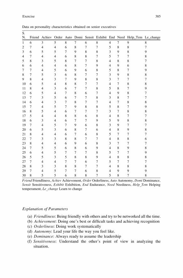
Explanation of Parameters
(a) Friendliness: Being friendly with others and try to be networked all the time.
(b) Achievement: Doing one’s best or difficult tasks and achieving recognition
(c) Orderliness: Doing work systematically
(d) Autonomy: Lead your life the way you feel like.
(e) Dominance: Always ready to assume the leadership
(f) Sensitiveness: Understand the other’s point of view in analyzing the
situation.
Data on personality characteristics obtained on senior executives
S.
N. Friend Achiev Order Auto Domi Sensit Exhibit End Need Help_Tem Le_change
1 6 3 5 8 7 6 8 4 7 9 8
2 7 4 4 6 8 7 7 5 8 8 7
3 6 5 5 7 9 8 8 3 9 8 9
4 7 4 4 6 8 8 7 5 7 7 8
5 8 3 5 8 7 7 8 4 8 8 7
6 6 4 4 6 8 7 9 4 9 6 8
7 7 4 5 6 9 6 8 5 8 7 9
8 7 5 3 6 8 7 7 3 9 8 8
9 8 4 3 7 9 8 8 3 7 7 7
10 6 5 4 8 8 7 7 4 7 8 8
11 8 4 3 6 7 7 8 5 8 7 9
12 6 5 4 7 8 6 7 4 9 8 7
13 7 3 5 6 7 7 8 3 8 7 7
14 6 4 3 7 8 7 7 4 7 8 8
15 7 4 5 7 9 8 8 5 8 7 9
16 8 5 4 6 7 7 7 3 7 8 8
17 5 4 4 8 8 6 8 4 8 7 7
18 6 3 4 6 7 7 9 5 9 8 8
19 7 4 5 7 9 6 8 3 9 7 7
20 6 5 3 6 8 7 6 4 8 9 8
21 8 4 4 6 7 6 8 5 7 7 7
22 7 3 3 8 8 7 7 4 8 8 6
23 8 4 4 6 9 6 8 3 7 7 7
24 7 5 5 6 8 6 9 4 8 9 8
25 6 4 5 7 7 7 8 5 7 7 9
26 5 5 3 5 8 8 9 4 8 8 8
27 7 4 4 7 7 6 7 5 7 7 7
28 8 3 3 8 8 7 7 4 8 8 8
29 7 4 5 7 7 6 8 4 9 9 9
30 8 5 5 6 8 8 7 5 8 7 8
Friend Friendliness, Achiev Achievement, Order Orderliness, Auto Autonomy, Domi Dominance,
Sensit Sensitiveness, Exhibit Exhibition, End Endurance, Need Neediness, Help_Tem Helping
temperament, Le_change Learn to change
Exercise 385

(g) Exhibition: To showcase one’s self by appearance, speech, and manner for
attracting others.
(h) Endurance: Being focus toward work until it is completed and being able to
work without being distracted.
(i) Neediness: Always ready to take support of others with grace and remains
obliged for that.
(j) Helping temperament: Always ready to help the needy and less fortunate.
(k) Learn to change: Always ready to change due to change environment.
2. A researcher wants to know the factors that are responsible for people to choose
the Rajdhani Express at different routes in India. Twenty respondents who
recently traveled from this train were selected for getting their responses.
These subjects were given a questionnaire consisting of ten questions mentioned
below. They were asked to give their opinion on a seven-point scale where 1
indicates complete agreement and seven complete disagreements. The responses
so obtained are shown in the following table.
Apply factor analysis and use varimax rotation to discuss your findings. Explain
the factors so extracted in the study.
Questionnaire includes
1. The attendants are caring
2. The bedding provided in the train is neat and clean.
Response data obtained from the passengers on the services provided during journey in the train
S.
N.
1.
Caring
2.
Bedding
3.
Courteous
4.
Food
5.
Spray
6.
Toilets
7.
Timeliness
8.
Seats
9.
Clean
10.
Snacks
1 2 2 1 2 3 4 2 2 4 1
2 3 1 2 3 2 5 4 2 5 2
3 4 2 4 4 3 6 4 3 6 3
4 1 1 2 3 2 4 3 2 4 2
5 2 2 3 4 2 4 4 3 3 3
6 3 2 2 3 3 3 3 2 3 2
7 4 1 3 6 2 5 5 1 5 5
8 5 1 5 5 3 6 5 2 6 4
9 5 1 2 2 2 5 3 2 5 1
10 3 2 3 2 2 5 3 3 5 2
11 6 1 4 4 2 4 4 2 6 3
12 6 2 6 3 3 6 3 3 6 2
13 2 5 3 4 6 5 4 6 4 3
14 1 2 3 3 3 4 4 3 2 2
15 3 1 2 4 3 5 5 2 3 3
16 4 5 3 4 5 4 5 6 4 3
17 2 2 2 1 3 3 3 3 5 1
18 2 1 3 3 2 3 4 2 6 2
19 1 2 2 3 3 4 3 3 2 2
20 3 1 1 1 4 2 2 2 3 1
386 11 Application of Factor Analysis: To Study the Factor Structure Among Variables

3. The ticket checkers are very courteous.
4. The quality of food is good.
5. To done away the foul smell fresheners are sprayed.
6. Toilets are always clean.
7. Foods are provided timely during the journey.
8. Seats are very comfortable.
9. Surroundings are clean all the time clean.
10. Vendors keep providing fresh and hot snacks all the time.
Answers of Multiple-Choice Questions
Q.1 b Q.2 c Q.3 c Q.4 b
Q.5 c Q.6 a Q.7 d Q.8 a
Q.9 c Q.10 d Q.11 a Q.12 c
Q.13 b Q.14 a
Exercise 387

Chapter 12
Application of Discriminant Analysis:
For Developing a Classification Model
Learning Objectives
After completing this chapter, you should be able to do the following:
• Understand the importance of discriminant analysis in research.
• List down the research situation where discriminant analysis can be used.
• Understand the importance of assumptions used in discriminant analysis.
• Know the different concepts used in discriminant analysis.
• Understand the steps involved in using SPSS for discriminant analysis.
• To interpret the output obtained in discriminant analysis.
• Explain the procedure in developing the decision rule using discriminant model.
• Know to write the results of discriminant analysis in standard format.
Introduction
Often we come across a situation where it is interesting to know as to why the two
naturally occurring groups are different. For instance, after passing the school, the
students can opt for continuing further studies, or they may opt for some skill-
related work. One may be interested to know as to what makes them to choose their
course of action. In other words, it may be desired to know on what parameters
these two groups may be distinct. Similarly one may like to identify the parameters
which distinguish the liking of two brands of soft drink by the customers or which
make the engineering and management students different. Thus, to identify the
independent parameters responsible for discriminating these two groups, a statisti-
cal technique known as discriminant analysis (DA) is used. The discriminant
analysis is a multivariate statistical technique used frequently in management,
social sciences, and humanities research. There may be varieties of situation
where this technique can play a major role in decision-making process. For
instance, the government is very keen that more and more students should opt for
the science stream in order to have the technological advancement in the country.
J.P. Verma, Data Analysis in Management with SPSS Software,DOI 10.1007/978-81-322-0786-3_12, # Springer India 2013
389
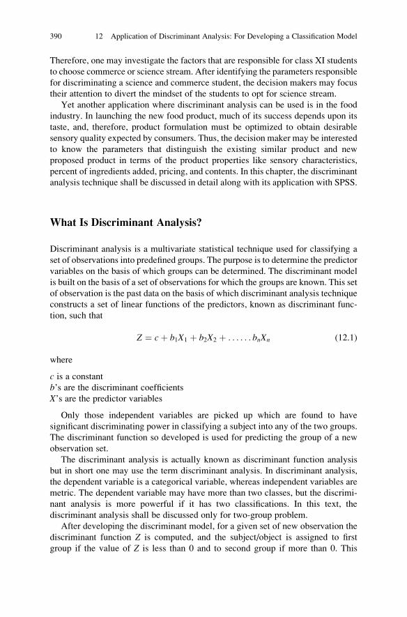
Therefore, one may investigate the factors that are responsible for class XI students
to choose commerce or science stream. After identifying the parameters responsible
for discriminating a science and commerce student, the decision makers may focus
their attention to divert the mindset of the students to opt for science stream.
Yet another application where discriminant analysis can be used is in the food
industry. In launching the new food product, much of its success depends upon its
taste, and, therefore, product formulation must be optimized to obtain desirable
sensory quality expected by consumers. Thus, the decision maker may be interested
to know the parameters that distinguish the existing similar product and new
proposed product in terms of the product properties like sensory characteristics,
percent of ingredients added, pricing, and contents. In this chapter, the discriminant
analysis technique shall be discussed in detail along with its application with SPSS.
What Is Discriminant Analysis?
Discriminant analysis is a multivariate statistical technique used for classifying a
set of observations into predefined groups. The purpose is to determine the predictor
variables on the basis of which groups can be determined. The discriminant model
is built on the basis of a set of observations for which the groups are known. This set
of observation is the past data on the basis of which discriminant analysis technique
constructs a set of linear functions of the predictors, known as discriminant func-
tion, such that
Z ¼ cþ b1X1 þ b2X2 þ . . . . . . bnXn (12.1)
where
c is a constantb’s are the discriminant coefficients
X’s are the predictor variables
Only those independent variables are picked up which are found to have
significant discriminating power in classifying a subject into any of the two groups.
The discriminant function so developed is used for predicting the group of a new
observation set.
The discriminant analysis is actually known as discriminant function analysis
but in short one may use the term discriminant analysis. In discriminant analysis,
the dependent variable is a categorical variable, whereas independent variables are
metric. The dependent variable may have more than two classes, but the discrimi-
nant analysis is more powerful if it has two classifications. In this text, the
discriminant analysis shall be discussed only for two-group problem.
After developing the discriminant model, for a given set of new observation the
discriminant function Z is computed, and the subject/object is assigned to first
group if the value of Z is less than 0 and to second group if more than 0. This
390 12 Application of Discriminant Analysis: For Developing a Classification Model
criterion holds true if an equal number of observations are taken in both the groups
for developing a discriminant function. However, in case of unequal sample size,
the threshold may vary on either side of zero.
The main purpose of a discriminant analysis is to predict group membership
based on a linear combination of the predictive variables. In using this technique,
the procedure starts with a set of observations where both group membership and
the values of the interval variables are known. The end result of the procedure is a
model that allows prediction of group membership when only the interval variables
are known.
A second purpose of the discriminant analysis is to study the relationship
between group membership and the variables used to predict group membership.
This provides information about the relative importance of independent variables in
predicting group membership.
Discriminant function analysis is similar to the ordinary least square (OLS)
regression analysis. The only difference is in the nature of dependent variable.
In discriminant function analysis, the dependent variable is essentially a categorical
(preferably dichotomous) variable, whereas in multiple regression it is a continuous
variable. Other differences are in terms of the assumptions being satisfied in using
discriminant analysis which shall be discussed later in this chapter.
Terminologies Used in Discriminant Analysis
Discriminant analysis provides discriminant function which is used to classify an
individual or cases into two categories on the basis of the observations on the
predictor variables. If the discriminant model developed in the analysis is robust for
a set of data, the percentage of correct classification of cases in the classification
table increases. To understand the application of discriminant analysis using SPSS
on any data set, it is essential to know its basics.
Variables in the Analysis
In discriminant analysis, the dependent variable is categorical in nature. It may have
two or more categories. The procedure used in discriminant analysis becomes very
complicated if the dependent variable has more than two categories. Further the
efficiency of the model also decreases in that case. The model becomes very
powerful if the dependent variable has only two categories. The dependent variable
is also known as criterion variable. In SPSS, dependent variable is known as
grouping variable. It is the object of classification on the basis of independent
variables.
The independent variables in the discriminant analysis are always metric.
In other words, the data obtained on the independent variables must be measured
Terminologies Used in Discriminant Analysis 391
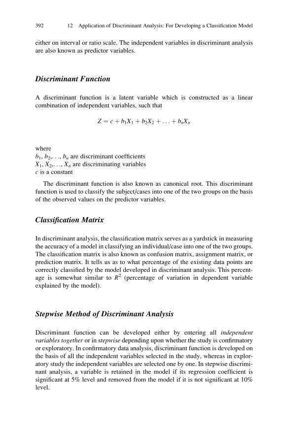
either on interval or ratio scale. The independent variables in discriminant analysis
are also known as predictor variables.
Discriminant Function
A discriminant function is a latent variable which is constructed as a linear
combination of independent variables, such that
Z ¼ cþ b1X1 þ b2X2 þ . . .þ bnXn
where
b1, b2,. . ., bn are discriminant coefficients
X1, X2,. . ., Xn are discriminating variables
c is a constant
The discriminant function is also known as canonical root. This discriminant
function is used to classify the subject/cases into one of the two groups on the basis
of the observed values on the predictor variables.
Classification Matrix
In discriminant analysis, the classification matrix serves as a yardstick in measuring
the accuracy of a model in classifying an individual/case into one of the two groups.
The classification matrix is also known as confusion matrix, assignment matrix, or
prediction matrix. It tells us as to what percentage of the existing data points are
correctly classified by the model developed in discriminant analysis. This percent-
age is somewhat similar to R2 (percentage of variation in dependent variable
explained by the model).
Stepwise Method of Discriminant Analysis
Discriminant function can be developed either by entering all independentvariables together or in stepwise depending upon whether the study is confirmatory
or exploratory. In confirmatory data analysis, discriminant function is developed on
the basis of all the independent variables selected in the study, whereas in explor-
atory study the independent variables are selected one by one. In stepwise discrimi-
nant analysis, a variable is retained in the model if its regression coefficient is
significant at 5% level and removed from the model if it is not significant at 10%
level.
392 12 Application of Discriminant Analysis: For Developing a Classification Model

Power of Discriminating Variables
After developing the model in discriminant analysis based on selected independent
variables, it is important to know the relative importance of the variables so
selected. This relative importance of the variable is determined by the coefficient
of the discriminating variable in the discriminant function. SPSS provides these
coefficients in the output and are named as standardized canonical discriminant
function coefficients. The higher the value of coefficient, the better is the discrimi-
nating power.
Box’s M Test
While applying ANOVA, one of the assumptions was that the variances are
equivalent for each group, but in DA the basic assumption is that the variance-
covariance matrices are equivalent. By using Box’s M tests, we test a null hypothe-
sis that the covariance matrices do not differ between groups formed by the
dependent variable. The researcher would not like this test to be significant so
that the null hypothesis that the groups do not differ can be retained. Thus, if the
Box’s M test is insignificant, it indicates that the assumptions required for DA holds
true.
However, with large samples, a significant result of Box’s M is not regarded as
too important. Where three or more groups exist, and Box’s M is significant, groups
with very small log determinants should be deleted from the analysis.
Eigenvalues
Eigenvalue is the index of overall model fit. It provides information on each of the
discriminant functions (equations) produced. In discriminant analysis, the maxi-
mum number of discriminant functions produced is the number of groups minus 1.
In case dependent variable has two categories, only one discriminant function shall
be generated. In DA, one tries to predict the group membership from a set of
predictor variables. If the dependent variable has two categories and there are npredictive variables, then a linear discriminant equation, Zi ¼ cþ b1X1 þ b2X2 þ. . .þ bnXn, is constructed such that the two groups differ as much as possible on Z.Here, one tries to choose the weights b1, b2,. . ., bn in computing a discriminant
score (Zi) for each subject so that if an ANOVA on Z is done, the ratio of the
between groups sum of squares to the within groups sum of squares is as large as
possible. The value of this ratio is known as eigenvalue.
Thus, eigenvalue is computed with the data on Z and is a quantity maximized by
the discriminant function coefficients.
Terminologies Used in Discriminant Analysis 393
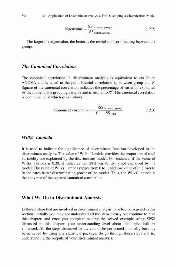
Eigenvalue ¼ SSBetween groups
SSWithin groups
(12.2)
The larger the eigenvalue, the better is the model in discriminating between the
groups.
The Canonical Correlation
The canonical correlation in discriminant analysis is equivalent to eta in an
ANOVA and is equal to the point biserial correlation rb between group and Z.Square of the canonical correlation indicates the percentage of variation explained
by the model in the grouping variable and is similar to R2. The canonical correlation
is computed on Z which is as follows:
Canonical correlation ¼ffiffiffiffiffiffiffiffiffiffiffiffiffiffiffiffiffiffiffiffiffiffiffiffiffiffiffiffiffiSSBetween groups
SSTotal
r(12.3)
Wilks’ Lambda
It is used to indicate the significance of discriminant function developed in the
discriminant analysis. The value of Wilks’ lambda provides the proportion of total
variability not explained by the discriminant model. For instance, if the value of
Wilks’ lambda is 0.28, it indicates that 28% variability is not explained by the
model. The value of Wilks’ lambda ranges from 0 to 1, and low value of it (closer to
0) indicates better discriminating power of the model. Thus, the Wilks’ lambda is
the converse of the squared canonical correlation.
What We Do in Discriminant Analysis
Different steps that are involved in discriminant analysis have been discussed in this
section. Initially you may not understand all the steps clearly but continue to read
this chapter, and once you complete reading the solved example using SPSS
discussed in this chapter, your understanding level about this topic shall be
enhanced. All the steps discussed below cannot be performed manually but may
be achieved by using any statistical package. So go through these steps and try
understanding the outputs of your discriminant analysis.
394 12 Application of Discriminant Analysis: For Developing a Classification Model

1. The first step in the discriminant analysis is to identify the independent variables
having significant discriminant power. This is done by taking all the independent
variables together in the model or one by one. The option for these two methods
can be seen in SPSS as “Enter independents together” and “Use stepwisemethod,” respectively.In stepwise method, an independent variable is entered in the model if its
corresponding regression coefficient is significant at 5% level and excluded at
subsequent stages until and unless it is significant at 10% level. Thus, in
developing discriminant function, the model will enter only significant indepen-
dent variables. The model so developed is required to be tested for its robustness.
2. In the second step, a discriminant function model is developed by using the
discriminant coefficients of the predictor variables and the value of constant
shown in the “Unstandardized canonical discriminant function coefficients”table generated in the SPSS output. This is similar to developing of regression
equation. This way, the function so generated may be used to classify an
individual into any of the two groups. The discriminant function shall look
like as follows:
Z ¼ cþ b1X1 þ b2X2 þ . . . . . . ::þ bnXn
where
Z is the discriminant function
X’s are predictor variables in the model
c is the constantb’s are the discriminant constants of the predictor variables
3. After developing discriminant model, the Wilks’ lambda is computed in the third
step for testing the significance of discriminant function developed in the model.
This indicates the robustness of discriminant model. The value of Wilks’ lambda
ranges from 0 to 1, and the lower value of it close to 0 indicates better discrimi-
nating power of the model. Further, significant value of chi-square indicates that
the discrimination between the two groups is highly significant.
After selecting independent variables as predictors in the discriminant model,
the model is tested for its significance in classifying the subjects/cases correctly
into groups. For this, SPSS generates a classification matrix. This is also known
as confusion matrix. This matrix shows the number of correct and wrong
classification of subjects in both the groups. High percentage of correct classifi-
cation indicates the validity of the model. The level of accuracy shown in the
classification matrix may not hold for all future classification of new subjects/
cases.
4. In the fourth step, the relative importance of predictor variables in discriminating
the two groups is discussed. The SPSS generates the “Standardized canonicaldiscriminant function coefficients” table. The variable with higher coefficient in
the table is the most powerful in discriminating the two groups, whereas the
variable having least coefficient indicates low discriminating power.
What We Do in Discriminant Analysis 395
5. Finally, a criterion for classification is developed on the basis of the midpoint of
the mean value of the transformed groups obtained in the table titled “Functionsat group centroids” generated in the SPSS output. If the value of the function Zcomputed on the basis of the equation developed in step 2 is less than this
midpoint, the subject is classified in one group and if it is more than it is
classified in second group.
Assumptions in Using Discriminant Analysis
While applying discriminant analysis, one should test the assumptions used in this
analysis. Following are the assumptions which are required to be fulfilled while
using this analysis:
1. Each of the independent variables is normally distributed. This assumption can
be examined by the histograms of frequency distributions. In fact, violations of
the normality assumption are usually not serious because in that case the
resultant significance tests are still reliable. One may use specific tests like
skewness and kurtosis for testing the normality in addition to graphs.
2. All variables have linear and homoscedastic relationships. It is assumed that the
variance/covariance matrices of variables are homogeneous in both the groups.
Box M test is used for testing the homogeneity of variances/covariances in both
the groups. However, it is sensitive to deviations from multivariate normality
and should not be taken too seriously.
3. Dependent variable is a true dichotomy. The continuous variable should never
be dichotomized for the purpose of applying discriminant analysis.
4. The groups must be mutually exclusive, with every subject or case belonging to
only one group.
5. All cases must be independent. One should not use correlated data like before-
after and matched pair data.
6. Sample sizes of both the groups should not differ to a great extent. If the sample
sizes are in the ratio 80:20, logistic regression may be preferred.
7. Sample size must be sufficient. As a guideline, there should be at least five to six
times as many cases as independent variables.
8. No independent variables should have a zero variability in either of the groups
formed by the dependent variable.
9. Outliers should not be present in the data. To solve this problem, inspect
descriptive statistics.
Research Situations for Discriminant Analysis
The discriminant analysis is used to develop a model for discriminating the future
cases/objects into one of the two groups on the basis of predictor variables. Hence,
it is widely used in the studies related to management, social sciences, humanities,
396 12 Application of Discriminant Analysis: For Developing a Classification Model

and other applied sciences. Some of the research situations where this analysis can
be used are discussed below:
1. In a hospitality firm, the data can be collected on employees in two different job
classifications: (1) customer support personnel and (2) back office management.
The human resources manager may like to know if these two job classifications
require different personality types. Each employee may be tested by a battery of
psychological test which consists of a measure of socialization trait,
extrovertness, frustration level, and orthodox approach.
The model can be used to priorities the predictor variable which can be used to
identify the employees in different category during selection process. Further,
the model may be helpful in developing the training program for future
employees recruited in different categories.
2. A college authority might divide a group of past graduate students into two
groups: students who finished the economics honors program in 3 years and
those who did not. The discriminant analysis could be used to predict successful
completion of the honors program based on the independent variables like SAT
score, XII maths score, and age of the candidates. Investigating the prediction
model might provide insight as to how each predictor individually and in
combination predicted completion or noncompletion of the economics honors
program at the undergraduate level.
3. Amarketingmanagermay like to develop amodel on buying two different kinds of
toothpaste on the basis of the product and customer profiles. The independent
variables may consist of age and sex of the customer and contained quantity, taste,
price of the products, etc. The insight from the developed model may provide the
decisionmakers in the company to develop andmarket their products with success.
4. A social scientist may like to know the predictor variable which is responsible
for smoking. The data on variables like the age at which the first cigarette was
smoked and other reasons of smoking like self-image, peer pressure, and frus-
tration level can be studied to develop a model for classifying an individual into
smoker and nonsmoker. The knowledge so accrued from the developed model
may be used to start the ad campaign against smoking.
5. In medical research, one may like to predict whether patient would survive from
burn injury based on the combinations of demographic and treatment variables.
The predictor variables might include burn percentage, body parts involved, age,
sex, and time between incident and arrival at hospital. In such situations, the
discriminant model so developed would allow a doctor to assess the chances of
recovery based on predictor variables. The discriminant model might also give
insight into how the variables interact in predicting recovery.
Solved Example of Discriminant Analysis Using SPSS
Example 12.1 The marketing division of a bank wants to develop a policy for
issuing visa gold card to its customers through which one can shop and withdraw up
Solved Example of Discriminant Analysis Using SPSS 397

to Rs. 100,000 at a time for 30 days without any interest. Out of several customers,
only a handful number of customers are required to be chosen for such facility.
Thus, a model is required to be made on the basis of the existing practices for
issuing similar card to the customers on the basis of the following data. The data
was collected on 28 customers in the bank who were either issued or denied similar
card earlier. Apply discriminant analysis to develop a discriminant function for
issuing or denying the golden visa card to the customers on the basis of their profile.
Also test the significance of the model so obtained. Discuss the efficiency of
classification and relative importance of the predictor variables retained in the
model (Table 12.1).
SolutionHere it is required to do the following:
1. To develop a discriminant function for deciding whether a customer be issued a
golden credit card
Table 12.1 Account details of the customers
S.
N.
Credit
card
Average daily
balance last
1 year
Number of days
balance <50,000 last
1 year
Annual
income in
lakh
Family
size
Average number
of transaction/
month
1 Issued 68,098 2 36.52 4 8
2 Denied 43,233 12 26.45 3 13
3 Issued 50,987 0 25.6 5 11
4 Denied 39,870 31 26.85 5 12
5 Denied 37,653 51 25.65 6 11
6 Denied 35,347 48 28.45 5 14
7 Issued 65,030 1 22.45 2 4
8 Issued 72,345 0 42.34 5 6
9 Denied 34,534 32 31.9 4 8
10 Issued 87,690 1 30.45 6 15
11 Denied 43,563 4 28.45 5 10
12 Denied 50,879 6 24.8 6 9
13 Denied 58,034 1 24.45 5 12
14 Issued 76,345 0 29.45 6 3
15 Issued 69,067 3 34.24 4 11
16 Denied 43,008 5 54.45 4 8
17 Issued 75,437 2 28.76 8 20
18 Denied 34,009 8 34.25 4 14
19 Issued 52,409 4 31.45 4 7
20 Denied 51,654 4 31.8 3 13
21 Issued 64,065 2 25.67 5 10
22 Denied 49,003 4 33.45 2 7
23 Issued 65,030 1 25.63 4 15
24 Issued 59,024 2 32.52 5 12
25 Issued 75,007 0 28.45 3 8
26 Denied 46,342 12 34.54 5 15
27 Denied 56,803 1 32.76 4 17
28 Issued 59,034 3 26.87 3 8
398 12 Application of Discriminant Analysis: For Developing a Classification Model
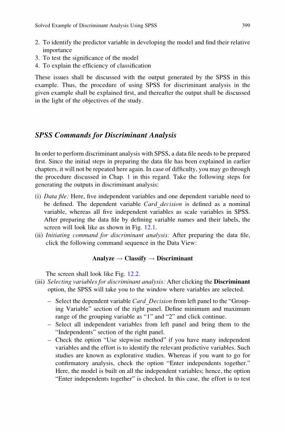
2. To identify the predictor variable in developing the model and find their relative
importance
3. To test the significance of the model
4. To explain the efficiency of classification
These issues shall be discussed with the output generated by the SPSS in this
example. Thus, the procedure of using SPSS for discriminant analysis in the
given example shall be explained first, and thereafter the output shall be discussed
in the light of the objectives of the study.
SPSS Commands for Discriminant Analysis
In order to perform discriminant analysis with SPSS, a data file needs to be prepared
first. Since the initial steps in preparing the data file has been explained in earlier
chapters, it will not be repeated here again. In case of difficulty, you may go through
the procedure discussed in Chap. 1 in this regard. Take the following steps for
generating the outputs in discriminant analysis:
(i) Data file: Here, five independent variables and one dependent variable need to
be defined. The dependent variable Card_decision is defined as a nominal
variable, whereas all five independent variables as scale variables in SPSS.
After preparing the data file by defining variable names and their labels, the
screen will look like as shown in Fig. 12.1.
(ii) Initiating command for discriminant analysis: After preparing the data file,
click the following command sequence in the Data View:
Analyze ! Classify ! Discriminant
The screen shall look like Fig. 12.2.
(iii) Selecting variables for discriminant analysis: After clicking the Discriminant
option, the SPSS will take you to the window where variables are selected.
– Select the dependent variable Card_Decision from left panel to the “Group-
ing Variable” section of the right panel. Define minimum and maximum
range of the grouping variable as “1” and “2” and click continue.
– Select all independent variables from left panel and bring them to the
“Independents” section of the right panel.
– Check the option “Use stepwise method” if you have many independent
variables and the effort is to identify the relevant predictive variables. Such
studies are known as explorative studies. Whereas if you want to go for
confirmatory analysis, check the option “Enter independents together.”
Here, the model is built on all the independent variables; hence, the option
“Enter independents together” is checked. In this case, the effort is to test
Solved Example of Discriminant Analysis Using SPSS 399

the model. Such studies are known as confirmatory studies. In this example,
all the variables have been selected to build the model. The screen will look
like Fig. 12.3.
(iv) Selecting the option for computation: After selecting variables, different
option needs to be defined for generating the output in discriminant analysis.
Take the following steps:
– Click the tag Statistics in the screen shown in Fig. 12.3. and
– Check the option of “Means” and “Box’s M” in the “Descriptives” section.
Fig. 12.1 Screen showing partial data file for the discriminant analysis in SPSS
400 12 Application of Discriminant Analysis: For Developing a Classification Model

– Check the options “Fisher’s” and “Unstandardized” in the “Function
Coefficients” section. The screen showing these options shall look like as
shown in Fig. 12.4.
– Press Continue. This will take you back to the screen shown in Fig. 12.3.
– Click the tag Classify in the screen as shown in screen 12.3. and
– Check the option “Summary table” in the Display section.
– Check the option “Casewise results” if you want to know wrongly classified
cases by the model.
The screen for these options shall look like Fig. 12.5.
– Click Continue.– Click OK for output.
(v) Getting the output: After clicking the OK option in Fig. 12.3, the output in the
discriminant analysis shall be generated in the output window. Selected outputs
can be copied in the word file by using the right click of the mouse over
identified area of the output. Out of many outputs generated by the SPSS, the
following relevant outputs have been picked up for discussion:
1. Group statistics including mean and standard deviation
Fig. 12.2 Screen showing SPSS commands for discriminant analysis
Solved Example of Discriminant Analysis Using SPSS 401
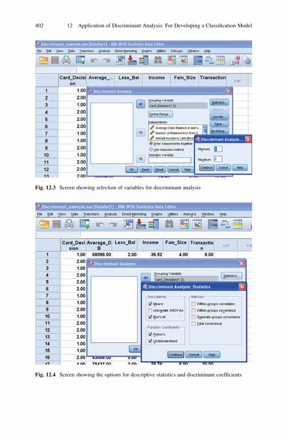
Fig. 12.3 Screen showing selection of variables for discriminant analysis
Fig. 12.4 Screen showing the options for descriptive statistics and discriminant coefficients
402 12 Application of Discriminant Analysis: For Developing a Classification Model

2. Unstandardized canonical discriminant function coefficients table
3. Eigen values and canonical correlation
4. Wilks’ lambda and chi-square test
5. Classification matrix
6. Standardized canonical discriminant function coefficients
7. Functions at group centroids
These outputs so generated by the SPSS are shown in Tables 12.2–12.8 and
Fig. 12.6.
Interpretation of Various Outputs Generated in DiscriminantAnalysis
The above-mentioned output so generated by the SPSS will now be discussed to
answer the issues raised in the example.
1. Table 12.2 shows descriptive statistics containing mean and standard deviation
for all the variables in both the groups, that is, card issued group and card denied
Fig. 12.5 Screen showing the options for classification matrix
Solved Example of Discriminant Analysis Using SPSS 403

group. The readers may draw relevant conclusions as per their objectives from
this table.
2. Table 12.3 reveals the value of unstandardized discriminant coefficients which
are used in constructing discriminant function. Since all independent variables
were included to develop the model, the discriminant coefficients of all the five
independent variables are shown in Table 12.3.
Thus, discriminant function can be constructed by using the values of constant
and coefficients of these five independent variables as shown in Table 12.3.
Z ¼ �4:253� :002� X2 � :028� X3 þ :017� X4 � :099� X5
where
X2 is number of balance less than 5,000 in last 1 year
X3 is annual income in lakh
X4 is family size
X5 is average transaction per month
Table 12.2 Group statistics: mean and standard deviation of all independent variables in different
groups
Issue decision Mean SD
Card issued Average daily balance in last 1 year 67,112.00 9989.74
Number of balance less than 5,000 in last 1 year 1.509 1.29
Annual income in lakh 30.03 5.19
Family size 4.57 1.50
Average transaction per month 9.86 4.62
Card denied Average daily balance in last 1 year 44,566.57 7923.67
Number of balance less than 5,000 in last 1 year 15.64 17.38
Annual income in lakh 31.30 7.56
Family size 4.36 1.15
Average transaction per month 11.64 2.95
Total Average daily balance in last 1 year 55,839.29 14,493.43
Number of balance less than 5,000 in last 1 year 8.5714 14.08
Annual income in lakh 30.67 6.39
Family size 4.46 1.32
Average transaction per month 10.75 3.91
Table 12.3 Unstandardized canonical discriminant function coefficients
Variables selected Function 1
Average daily balance in last 1 year (X1) .000
Number of balance less than 5,000 in last 1 year (X2) �.002
Annual income in lakh (X3) �.028
Family size (X4) .017
Average transaction per month (X5) �.099
Constant �4.253
404 12 Application of Discriminant Analysis: For Developing a Classification Model

3. The canonical correlation is 0.815 as shown in Table 12.4. This indicates that
approximately 66% of the variation in the two groups is explained by the
discriminant model.
Since the Wilks’ lambda provides the proportion of unexplained variance by the
model, the lesser its value, the better is the discriminant model. The value of
Wilks’ lambda lies in between 0 and 1. Its value here is 0.336 as shown in
Table 12.5; hence, the model can be considered good because only 33.6%
variability is not explained by the model. To test the significance of Wilks’
lambda, the value of chi-square is calculated which is shown in Table 12.5. Since
the p value associated with it is .000 which is less than .05, it may be inferred that
the model is good.
4. Table 12.6 is a classification matrix which shows the summary of correct and
wrong classification of cases in both the groups on the basis of the developed
discriminant model. This table shows that out of 14 customers whom credit card
was issued, 12 were correctly classified by the developed model and 2 were
wrongly classified in the card denied group. On the other hand, out of 14
customers whom card was denied, 13 were classified by the model correctly in
the card denied group and only 1 customer was wrongly classified in the card
issued group. Thus, out of 28 cases, 25 (89.3%) cases were correctly classified by
the model which is quite high; hence, the model can be considered as valid.
Since this model is developed on the basis of a small sample, the level of
accuracy shown in the classification matrix may not hold for all future classifi-
cation of new cases.
5. Table 12.7 shows the standardized discriminant coefficients of the independent
variables in the model. The magnitude of these coefficients indicates the dis-
criminating power of the variables in the model. The variable having higher
Table 12.4 Eigenvalues
Function Eigenvalue % of variance Cumulative % Canonical correlation
1 1.975a 100.0 100.0 .815aFirst 1 canonical discriminant functions were used in the analysis
Table 12.5 Wilks’ lambda
and chi-square testTest of function(s) Wilks’ lambda Chi-square df Sig.
1 .336 25.618 5 .000
Table 12.6 Classification resultsa
Predicted group membership
Issue decision Card issued Card denied Total
Original count Card issued 12 2 14
Card denied 1 13 14
% Card issued 85.7 14.3 100.0
Card denied 7.1 92.9 100.0a89.3% of original grouped cases correctly classified
Solved Example of Discriminant Analysis Using SPSS 405

magnitude of the absolute function value is more powerful in discriminating the
two groups. Since absolute function value of the variable average daily balancein last one year is .988 which is higher than that of the variable averagetransaction per month (.382), average daily balance is having more discriminat-
ing power than the average transaction per month. By careful examination, you
may notice that the coefficient of average daily balance is the maximum, and in
fact it is very large in comparison to other variables; hence, it may be concluded
that this is the most important variable in taking a decision to issue or not to issue
the golden visa card.
Remark: You may run the discriminant analysis on the same data by using the
option “Use stepwise method” in order to ascertain the fact, whether the variable
average daily balance gets selected in the model. You may also check as to how
much accuracy is reduced in the model if some of the independent variables are
dropped from the model.
6. One of the purposes of running discriminant analysis in this example was to
develop a decision model for classifying a customer into two categories, that is,
card issued and card denied. Table 12.8 shows the means for the transformed
group centroids. Thus, the new mean for group 1 (card denied) is�1.354 and for
group 2 (card issued) is +1.354. This indicates that the midpoint of these two is 0.
These two means can be plotted on a straight line by locating the midpoint as
shown in Fig. 12.6.
Figure 12.6 defines the decision rule for classifying any new customer into any
of the two categories. If the discriminant score of any customer falls to the right of
the midpoint (Z > 0), he/she is classified into the card issue category, and if it falls
to the left of the midpoint (Z < 0), he/she is classified into card denied category.
Table 12.7 Standardized
canonical discriminant
function coefficients
Variables selected Function 1
Average daily balance in last 1 year .988
Number of balance less than 5,000 in last 1 year �.019
Annual income in lakh �.184
Family size .023
Average transaction per month �.382
Table 12.8 Functions at group centroids
Issue decision Function 1
Card issued 1.354
Card denied �1.354
Unstandardized canonical discriminant functions evaluated at group means
406 12 Application of Discriminant Analysis: For Developing a Classification Model

Summary of the SPSS Commands for Discriminant Analysis
(i) After preparing the data file, follow the below-mentioned command sequence
for discriminant analysis:
Analyze Classify Discriminant
(ii) Select the dependent variable Card_Decision from left panel to the “Grouping
Variables” section of the right panel and define its minimum and maximum
range as “1” and “2.” Further, select all independent variables from the left
panel to the “Independents” section of the right panel. Check the option “Enter
independents together.”
(iii) Click the tag Statistics and check options for “Means,” “Fisher’s,” and
“Unstandardized” in it. Click Continue.(iv) Click the tag Classify and check option for “Summary table.” Press Continue.(v) Press OK for output.
Exercise
Short Answer Questions
Note:Write answer to each of the following questions in not more than 200 words.
Q.1. Explain a research situation where discriminant analysis can be used and
discuss its utility.
Q.2. In discriminant analysis, what dependent variable refers to? What is the data
type of dependent variable in SPSS?
Q.3. Discuss situations in which the discriminant analysis uses the two different
methods like “Enter independents together” and “Use stepwise method” fordeveloping the discriminant model.
Q.4. What do you mean by discriminating variables? What is its significance in
discriminant analysis?
Q.5. What is the significance of Box’s M test in discriminant analysis? What does
the magnitude of Box’s M signify?
Q.6. What do you mean by eigenvalues? Explain its importance.
Q.7. Explain the significance of canonical correlation. What does it convey?
Mean of group 1 Mean of group 2(Card denied) (Card issued)
_____________________________________________
-1.354 0 +1.354
Value of Z
Fig. 12.6 Means of the transformed group centroids
Exercise 407
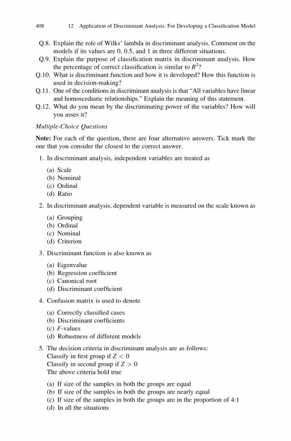
Q.8. Explain the role of Wilks’ lambda in discriminant analysis. Comment on the
models if its values are 0, 0.5, and 1 in three different situations.
Q.9. Explain the purpose of classification matrix in discriminant analysis. How
the percentage of correct classification is similar to R2?
Q.10. What is discriminant function and how it is developed? How this function is
used in decision-making?
Q.11. One of the conditions in discriminant analysis is that “All variables have linear
and homoscedastic relationships.” Explain the meaning of this statement.
Q.12. What do you mean by the discriminating power of the variables? How will
you asses it?
Multiple-Choice Questions
Note: For each of the question, there are four alternative answers. Tick mark the
one that you consider the closest to the correct answer.
1. In discriminant analysis, independent variables are treated as
(a) Scale
(b) Nominal
(c) Ordinal
(d) Ratio
2. In discriminant analysis, dependent variable is measured on the scale known as
(a) Grouping
(b) Ordinal
(c) Nominal
(d) Criterion
3. Discriminant function is also known as
(a) Eigenvalue
(b) Regression coefficient
(c) Canonical root
(d) Discriminant coefficient
4. Confusion matrix is used to denote
(a) Correctly classified cases
(b) Discriminant coefficients
(c) F-values(d) Robustness of different models
5. The decision criteria in discriminant analysis are as follows:
Classify in first group if Z < 0
Classify in second group if Z > 0
The above criteria hold true
(a) If size of the samples in both the groups are equal
(b) If size of the samples in both the groups are nearly equal
(c) If size of the samples in both the groups are in the proportion of 4:1
(d) In all the situations
408 12 Application of Discriminant Analysis: For Developing a Classification Model

6. In stepwise method of discriminant analysis, a variable is included in the model
if it is found significant at
(a) 2% level
(b) 1% level
(c) 10% level
(d) 5% level
7. The Wilks’ lambda indicates
(a) Percentage variability in the two groups explained by the model
(b) Robustness of the model
(c) Proportion of total variability not explained by the discriminant model
(d) Significance of discriminant coefficients
8. One of the assumptions in discriminant analysis is that
(a) All variables have curvilinear and homoscedastic relationships.
(b) All variables have linear and non-homoscedastic relationships.
(c) All variables have curvilinear and non-homoscedastic relationships.
(d) All variables have linear and homoscedastic relationships.
9. Correct sequence of commands in SPSS for discriminant analysis is
(a) Analyze ! Discriminant ! Classify
(b) Analyze ! Classify ! Discriminant
(c) Discriminant ! Analyze ! Classify
(d) Discriminant ! Classify ! Analyze
10. Value of Wilks’ lambda ranges from
(a) �1 to +1
(b) 0 to 1
(c) �1 to 0
(d) �2 to 2
11. Discriminant function is developed on the basis of
(a) Standardized coefficients
(b) Unstandardized coefficients
(c) Classification matrix
(d) Functions at group centroids
12. The power of discrimination of an independent variable is determined by
(a) Unstandardized canonical coefficients
(b) Wilks’ lambda
(c) Standardized canonical coefficients
(d) Eigenvalues
Exercise 409

13. In explorative discriminant analysis,
(a) All the independent variables are taken in the study.
(b) Only those variables which are known to have sufficient discriminating
power are taken in the study.
(c) Maximum number of relevant independent variables are taken in the study.
(d) It is up to researcher to identify the independent variables in the study.
14. Choose the correct statement in discriminant analysis.
(a) Dependent variable is an ordinal variable.
(b) The groups should not be mutually exclusive.
(c) Sample sizes should differ to a great extent.
(d) No independent variables should have a zero variability in either of the
groups formed by the dependent variable.
15. In discriminant analysis, the square of the canonical correlation is an indicator
of
(a) Relationship among the independent variables
(b) Efficiency of the predictor variables
(c) Discriminating power of the independent variables
(d) The percentage of variability explained by the predictor variables in the
two groups
Assignments
1. A study was conducted to know the variables responsible for selection in the
bank probationary officers examination. Thirty candidates who appeared in the
examination were identified for the study, and following data were obtained on
them.
Results of the examination and subject’s profile
S.N. Bank examination result IQ English Numerical aptitude Reasoning
1 Successful 78 56 65 78
2 Successful 76 76 76 89
3 Not successful 74 52 63 93
4 Not successful 65 49 62 90
5 Successful 83 71 82 85
6 Successful 79 80 86 84
7 Not successful 91 54 52 89
8 Not successful 64 65 53 84
9 Not successful 53 69 54 85
10 Successful 60 78 75 92
11 Not successful 65 69 63 83
12 Successful 86 73 83 83
13 Not successful 53 65 67 83
14 Successful 74 69 80 78
15 Successful 60 68 81 74
16 Successful 75 75 78 85
(continued)
410 12 Application of Discriminant Analysis: For Developing a Classification Model

(continued)
Results of the examination and subject’s profile
S.N. Bank examination result IQ English Numerical aptitude Reasoning
17 Not successful 56 73 75 83
18 Not successful 65 64 56 84
19 Not successful 56 58 64 86
20 Successful 95 68 78 82
21 Successful 92 80 74 83
22 Not successful 45 73 71 91
23 Successful 85 56 89 74
24 Successful 68 45 83 85
25 Not successful 64 73 64 84
26 Not successful 70 71 56 86
27 Successful 78 74 84 94
28 Not successful 64 70 55 86
29 Not successful 42 67 51 76
30 Successful 82 67 90 83
Develop a discriminant model. Test the significance of the developed model and
find the relative importance of the independent variables in the model. Compare
the efficiency of the two discriminant function models obtained by taking all the
variables at once and stepwise methods.
2. A branded apparel company wanted to reward its loyal customers by means of
incentives in the form of 60% discount in the first week of New Year. The
company had a loose policy of identifying a customer into loyal or disloyal on
the basis of certain criterion which was more subjective. However, the manage-
ment was interested to develop a more scientific approach to build up a model of
classifying a customer into loyal and disloyal group. A sample of 30 customers
were chosen from the database, and their purchase details were recorded which
are shown in the following table:
Apply discriminant analysis to build up a classification model which can be used
for the existing and future customers to reward as per the company policy. Test
Purchase data of the customers of the apparel company
S.
N.
Customer
classification
No. of purchases/
year in a year
Purchase
amount in a
year
No. of kids’ wear
apparel/year
No. of ladies
apparel/year
No. of
gents
1 Loyal 6 109,870 23 12 2
2 Disloyal 8 27,000 4 8 18
3 Loyal 11 135,000 22 23 11
4 Loyal 15 12,340 12 5 4
5 Disloyal 9 54,000 20 23 8
6 Disloyal 4 34,000 12 8 20
7 Loyal 8 98,000 16 9 22
8 Loyal 8 80,002 23 25 3
9 Disloyal 4 71,000 25 15 19
10 Loyal 8 180,000 35 24 12
(continued)
Exercise 411

the significance of discriminant function, explain the percentage of correct
classification by the model, and discuss the relative importance of independent
variable. Find out the percentage of variability explained by the discriminant
model in both the situations when all the variables are included in the model and
when the variables are identified using stepwise procedure.
Hint: In Assignment 2, since the number of scores in loyal and disloyal customer
groups are not same, you may not get mean of Z as 0. In this example, you will get the
new mean for group 1 (Disloyal group) as �1.603 and new mean for group 2 (Loyal
group) as 1.403. Thus,midpoint of these groupswould be�.1 instead of 0.A customer
would be classified as disloyal or loyal depending upon Z < �.1 or Z > �.1.
Answers to Multiple-Choice Questions
Q.1 a Q.2 c
Q.3 c Q.4 a
Q.5 a Q.6 d
Q.7 c Q.8 d
Q.9 b Q.10 b
Q.11 b Q.12 c
Q.13 c Q.14 d
Q.15 d
(continued)
S.
N.
Customer
classification
No. of purchases/
year in a year
Purchase
amount in a
year
No. of kids’ wear
apparel/year
No. of ladies
apparel/year
No. of
gents
11 Disloyal 6 34,012 3 2 15
12 Loyal 12 67,000 12 8 5
13 Loyal 5 92,008 20 12 9
14 Disloyal 4 12,000 6 2 8
15 Loyal 10 71,540 6 15 8
16 Disloyal 4 13,450 1 2 15
17 Loyal 14 125,000 24 15 8
18 Loyal 20 80,000 5 20 7
19 Disloyal 5 56,021 15 10 15
20 Loyal 9 170,670 21 25 12
21 Disloyal 6 1,012 1 1 1
22 Disloyal 7 54,276 13 8 15
23 Loyal 15 100,675 25 25 5
24 Loyal 12 106,750 30 15 4
25 Disloyal 11 3,500 2 2 3
26 Disloyal 5 2,500 2 1 3
27 Loyal 10 89,065 14 21 8
28 Loyal 9 80,540 15 19 16
29 Disloyal 7 12,000 4 4 6
30 Disloyal 3 5,056 4 2 3
412 12 Application of Discriminant Analysis: For Developing a Classification Model
Chapter 13
Logistic Regression: Developing a Model
for Risk Analysis
Learning Objectives
After completing this chapter, you should be able to do the following:
• Learn the difference between logistic regression and ordinary least squares
regression.
• Know the situation where logistic regression can be used.
• Describe the logit transformation used in the analysis.
• Understand different terminologies used in logistic regression.
• Explain the steps involved in logistic regression.
• Understand the assumptions used in the analysis.
• Know the SPSS procedure involved in logistic regression.
• Understand the odds ratio and its use in interpreting the findings.
• Interpret the outputs of logistic regression generated by the SPSS.
Introduction
Logistic regression is a useful statistical technique for developing a prediction
model for any event that is binary in nature. A binary event can either occur or
not occur. It has only two states which may be represented by 1(occurrence) and 0
(nonoccurrence). Logistic regression can also be applied in a situation where the
dependent variable has more than two classifications. The logistic regression can
either be binary or multinomial depending upon whether the dependent variable is
classified into two groups or more than two groups, respectively. In this chapter, the
discussion shall be made only for binary logistic regression.
Logistic regression is useful in a situation where we are interested to predict the
occurrence of any happening. It has vast application in the area of management,
medical and social researches because in all these discipline occurrence of a
phenomenon depends upon the independent variables that are metric as well as
categorical in nature. Logistic regression can be used for developing model for
J.P. Verma, Data Analysis in Management with SPSS Software,DOI 10.1007/978-81-322-0786-3_13, # Springer India 2013
413

financial prediction, bankruptcy prediction, buying behavior, fund performance,
credit risk analysis, etc. We have witnessed the failure of high-profile companies in
the recent past. This has generated an interest among the industrial researcher to
develop a model for bankruptcy prediction. Such model can also be made for retail
and other firms on the basis of the accounting variables such as inventories,
liabilities, receivables, net income (loss), and revenue. On the basis of such
model, one can estimate the risk of bankruptcy of any organization.
In hilly regions, there is always a fear of landslide which causes heavy damage to
the infrastructure and human lives. The logistic regression model can be used to find
out the landslide susceptibility in such areas. The model can identify more probable
areas prone to landslides. On the basis of such information, appropriate measures may
be taken to reduce the risk from potential landslide hazard. In developing the logistic
model for landslide susceptibility, the remote sensing and geographic information
system (GIS) data may be used as independent variables.
In product marketing, it is required to identify those customers on whom adver-
tisement should be focused. Consider a situation in which a company has introduced
an herbal cream costing Rs. 520 and wishes to identify the parameters responsible for
the customers to buy this product. The data on the parameters like age, gender,
income, and family size may be collected on the customers who have inspected the
cream at the counter in few stores. Here the dependent variable is the buying decision
of the customer (1 if the cream is purchased and 0 if not), whereas the independent
variables are the mix of ratio (age, income, family size) and categorical variable
(gender). Since the dependent variable is the dichotomous variable and independent
variables have a combination of ratio and categorical variables, the logistic regression
can be applied to identify the variables that are responsible for the buying behavior of
the customers. Further, the relative importance of the independent variable can also
be known by this analysis, and therefore, decision maker may focus on those
variables which maximize the chances of buying the product.
In the financial sector, financial companies may be interested to find the attributes
of the financial managers responsible for fund performance. One may investigate by
using logistic model as to which of the independent variables out of educational
background, gender, and seniority of the fund managers are related with the fund
performance.
Due to large number of listed companies on the bourses, there is always a fear of
credit issues and frequent credit crises. The logistic model may be developed for
credit risk analysis which may provide the monitoring agency a system of identifying
corporate financial risk which works as an effective indicator system. In developing
such model, the past data is usually taken on the identified parameters.
What Is Logistic Regression?
Logistic regression is a kind of predictive model that can be used when the
dependent variable is a categorical variable having two categories and independent
variables are either numerical or categorical. Examples of categorical variables are
414 13 Logistic Regression: Developing a Model for Risk Analysis
buying/not buying a product, disease/no disease, cured/not cured, survived/not
survived, etc. The logistic regression is also known as logit model or logistic model.
The dependent variable in the logit model is often termed as outcome or target
variable, whereas independent variables are known as predictive variables. A logistic
regression model is more akin to nonlinear regression such as fitting a polynomial to a
set of data values. By using the logistic model, the probability of occurrence of an
event is predicted by fitting data to a logit function or a logistic curve.
Important Terminologies in Logistic Regression
Before getting involved into serious discussion about the logistic regression, one
must understand different terminologies involved in it. The terms which are
required in understanding the logistic regression are discussed herewith.
Outcome Variable
Outcome variable is that variable in which a researcher is interested. In fact it is a
dependent variable which is binary in nature. The researcher is interested to know
the probability of its happening on the basis of several risk factors. For example, the
variables like buying decision (buying ¼ 1, not buying ¼ 0), survival (surviving
¼ 1, not surviving ¼ 0), bankruptcy (bankruptcy of an organization ¼ 1, no bank-
ruptcy ¼ 0), and examination results (pass ¼1, fail ¼ 0) are all outcome variables.
Natural Logarithms and the Exponent Function
The natural log is the usual logarithmic function with base e. The natural log of X is
written as log(X) or ln(X). On the other hand, the exponential function involves the
constant “e” whose value is equal to 2.71828182845904 (�2.72). The exponential
of X is written as exp(x) ¼ ex. Thus, exp(4) equals to 2.724 ¼ 54.74.
Since natural log and exponential function are opposite to each other,
E4 ¼ 54:74
) ln 54:74ð Þ ¼ 4
Important Terminologies in Logistic Regression 415
Odds Ratio
If probability of success (p) of any event is 0.8, then the probability of its failure is
(1 � p) ¼ 1�0.8 ¼ 0.2. The odds of the success can be defined as the ratio of the
probability of success to the probability of failure. Thus, in this example, odds of
success is 0.8/0.2 ¼ 4. In other words, the odds of success is 4 to 1. If the
probability of success is 0.5, then the odds of success is 1 and it may be concluded
that the odds of success is 1 to 1.
In logistic regression, odds ratio can be obtained by finding the exponential of
regression coefficient, exp(B), and is sometimes written as eB. If the regression
coefficient B is equivalent to 0.80, then the odds ratio will be 2.40 because exp
(0.8) ¼ 2.4.
The odds ratio of 2.4 indicates that the probability of Y equals to 1 is 2.4 times as
likely as the value of X is increased by one unit. If an odds ratio is .5, it indicates that
the probability of Y ¼ 1 is half as likely with an increase of X by one unit (here
there is a negative relationship between X and Y). On the other hand, the odds ratio
1.0 indicates that there is no relationship between X and Y.The odds ratio can be better understood if both variables Y and X are dichoto-
mous. In that case, the odds ratio can be defined as the probability that Y is 1 when Xis 1 compared to the probability that Y is 1 when X is 0. If the odds ratio is given,
then B coefficient can be obtained by taking the log of the odds ratio. It is so because
log and exponential functions are opposite to each other.
The transformation from probability to odds is a monotonic transformation.
It means that the odds increases as the probability increases or vice versa. Proba-
bility ranges from 0 to 1, whereas the odds ranges from 0 to positive infinity.
Similarly the transformation from odds to log of odds, known as log transforma-
tion, is also a monotonic transformation. In other words, the greater the odds, the
greater is the log of odds and vice versa. Thus, if the probability of success
increases, the odds ratio and log odds both increase and vice versa.
Maximum Likelihood
Maximum likelihood is the method of finding the least possible deviation between
the observed and predicted values using the concept of calculus specifically
derivatives. It is different than ordinary least squares (OLS) regression where we
simply try to find the best-fitting line by minimizing the squared residuals.
In maximum likelihood (ML) method, the computer uses different “iterations”
where different solutions are tried for getting the smallest possible deviations or
best fit. After finding the best solution, the computer provides the final value for the
deviance, which is denoted as “�2 log likelihood” in SPSS. Cohen et al. (2003)
called this deviance statistic as�2LL, whereas some other authors like Hosmer and
Lemeshow (1989) called it D. This deviance statistic follows the chi-square
distribution.
416 13 Logistic Regression: Developing a Model for Risk Analysis

The likelihood ratio test, D, is used as goodness-of-fit. This test is referred in
SPSS by “chi-square.” The significance of this test can be seen by looking to its
value in the chi-square table in the appendix using degrees of freedom equal to the
number of predictors.
Logit
The logit is a function which is equal to the log odds of a variable. If p is a
probability that Y ¼ 1(occurrence of an event), then p/(1 � p) is the correspondingodds. The logit of the probability p is given by
LogitðpÞ ¼ logp
1� p
� �(13.1)
In logistic regression, logit is a special case of a link function. In fact, this logit
serves as a dependent variable and is estimated from the model.
Logistic Function
A logistic curve is just like sigmoid curve and is obtained by the logistic function
given by
p ¼ f ðzÞ ¼ eZ
1þ eZ(13.2)
The shape of the curve is like a letter “S.” In logistic function, the argument z ismarked along horizontal axis and the value of the function f(z) along the vertical
axis (Fig. 13.1).
The main feature of this logistic function is that the variable Z can assume any
value from minus � 1 to + 1, but the outcome variable p can have the values
only in the range 0–1. This function is used in logistic regression model to find the
probability of occurring the target variable for a given value of independent
variables.
Logistic Regression Equation
The logistic regression equation is similar to the ordinary least squares (OLS)
regression equation with the only difference that the dependent variable here is
Important Terminologies in Logistic Regression 417

the log odds of the probability that the dependent variable Y ¼ 1. It is written as
follows:
logit ¼ lnp
1� p
� �¼ B0 þ B1X1 þ B2X2 þ ::::::::: þ BnXn (13.3)
where B0 is an intercept and B1, B2. . ..Bn are the regression coefficients of X1, X2
. . ...,Xn, respectively. The dependent variable in logistic regression is log odds,
which is also known as logit.
Since in logistic regression log odds acts as a dependent variable which is
regressed on the basis of the independent variables, interpretation of regression
coefficients is not as easy as in case of OLS regression. In case of OLS regression,
the regression coefficient b represents the change in Y with one unit change in X.This concept is not valid in case of logistic regression equation; instead the
regression coefficient b is converted into odds ratio to interpret the happening of
outcome variable. The interpretation of odds ratio has been discussed above in
detail under the heading “Odds Ratio.”
Judging the Efficiency of the Logistic Model
In case of OLS regression equation, R2 used to be the measure of efficiency in
assessing the suitability of the model. But in case of logistic regression, this statistic
is no longer valid indicator of model robustness, because of the fact that the
dependent variable here is a binary variable. Thus, to assess the suitability of the
logistic model, we use the concept of deviance. In logistic regression, the chi-square
Fig. 13.1 Shape of the
logistic function
418 13 Logistic Regression: Developing a Model for Risk Analysis
is used as a measure of model fit instead of R2. It tells you about the fit of the
observed values (Y) to the expected values ( Y ). If the difference between the
observed values from the expected values increases, the fit of the model becomes
poorer. Thus, the effort is to have the deviance as small as possible. If more relevant
variables are added to the equation, the deviance becomes smaller, indicating an
improvement in fit.
Understanding Logistic Regression
In logistic regression, the approach of prediction is similar to that of ordinary least
squares (OLS). However, in logistic regression, a researcher predicts the probability
of an occurrence of a dependent variable which is binary in nature. Another
difference in logistic regression is that the independent variables can be a mix of
numerical and categorical. Due to dichotomous nature of the dependent variable,
assumptions of OLS that the error variances (residuals) are normally distributed are
not satisfied. Instead, they are more likely to follow a logistic distribution.
In using logistic distribution, one needs to make an algebraic conversion to
arrive at usual linear regression equation. In logistic regression, no standard solu-
tion is obtained and no straightforward interpretation can be made as is done in case
of OLS regression. Further, in logistic model, there is no R2 to measure the
efficiency of the model; rather a chi-square test is used to test how well the logistic
regression model fits the data.
Graphical Explanation of Logistic Model
Let us first understand the concept of logistic regression with one independent
variable. Consider a situation where we try to predict whether a customer would
buy a product(Y) depending upon the number of days(X) he saw the advertisement
of that product. It is assumed that the customers who watch the advertisement for
many days will be more likely to buy the product. The value of Y can be 1 if the
product is purchased by the customer and 0 if not.
Since the dependent variable is not a continuous, hence the goal of logistic
regression is to predict the likelihood that Y is equal to 1 (rather than 0) given
certain values of X. Thus, if there is a positive linear relationship between X and Y,then the probability that a customer will buy the product (Y ¼ 1) will increase with
the increase in the value of X (number of days advertisement seen). Hence, we are
actually predicting the probabilities instead of value of the dependent variable.
Understanding Logistic Regression 419

In this simulated experiment in investigating the behavior of 100 customers in
terms of buying the product of more than Rs. 1,000, their range of viewing the
advertisement for the number of days was from 0 to 15 days. We may plot the
probability that Y ¼ 1 with the increase in the value of X in terms of the graph. To
make it more convenient, let us club the number of advertisement-viewing days into
the categories 0–3, 4–6, 7–9, 10–12, and 13–15. Computing the mean score on Y(taking the average of 0s and 1s) for each category, the data would look like as
shown in Table 13.1.
If we plot these data, the graph would look like as shown in Fig. 13.2.
If we look at this graph, it looks like an S-shaped graph. If there is a strong
relationship between X and Y, the graph would be closer to perfect S-shaped unlike
the OLS regression where you get the straight line.
Table 13.1 Mean score for each category
No. of days advertisement viewing Probability that Y ¼ 1 (average of 0s and 1s in each category)
0–3 .17
4–6 .40
7–9 .50
10–12 .56
13–15 .96
Pro
babi
lity
of
buyi
ng(Y
= 1
)
0-4 0-3 4-6 7-9 10-12 13-15
No. of days advertisement seen (X)
0.5
0.0
1.0
Fig. 13.2 Graphical representation of the probability of buying versus number of days advertise-
ment seen
420 13 Logistic Regression: Developing a Model for Risk Analysis

Logistic Model with Mathematical Equation
If Y is the target variable (dependent) and X is the predictive variable and if the
probability that Y ¼ 1 is denoted asp_, then the probability that Y is 0 would be1� p
_.
The logistic model for predicting p_would be given by
lnp
1� p_
� �¼ B0 þ B1X (13.4)
where ln p1�p
� �is the log of the odds ratio and is known as logit and B0 is the
constant and B1 is the regression coefficient.
In effect, in logistic regression this logit, ln p1�p
� �, is the dependent variable
against which independent variables are regressed.
From Eq. (13.4), the probability ( p_) that Y ¼ 1 can be computed for a given
value of X.Let us assume that
Z ¼ lnp
1� p_
� �¼ B0 þ B1X (13.5)
)_p
1� p_¼ eZ
Or
p_ ¼ eZ
1þ eZ¼ eB0þB1X
1þ eB0þB1X(13.6)
Thus, in the logistic regression, first a logit or log of odds ratio, that is, ln p1�p
� �,
is computed for a given value of X, and then the probability (p_) that Y ¼ 1 is
computed by using formula (13.6). In fact (13.6) gives the logistic function as
f ðzÞ ¼ eZ
1þ eZ(13.7)
This function if plotted by taking z on horizontal axis and f(z) on vertical axis
looks like as shown in Fig. 13.3.
Understanding Logistic Regression 421
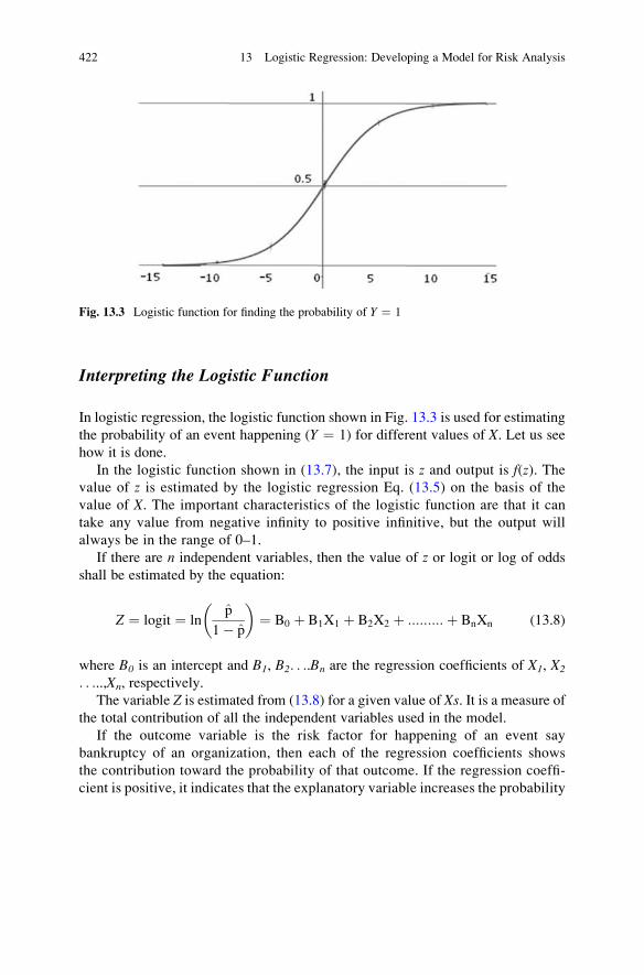
Interpreting the Logistic Function
In logistic regression, the logistic function shown in Fig. 13.3 is used for estimating
the probability of an event happening (Y ¼ 1) for different values of X. Let us seehow it is done.
In the logistic function shown in (13.7), the input is z and output is f(z). Thevalue of z is estimated by the logistic regression Eq. (13.5) on the basis of the
value of X. The important characteristics of the logistic function are that it can
take any value from negative infinity to positive infinitive, but the output will
always be in the range of 0–1.
If there are n independent variables, then the value of z or logit or log of odds
shall be estimated by the equation:
Z ¼ logit ¼ lnp
1� p
� �¼ B0 þ B1X1 þ B2X2 þ :::::::::þ BnXn (13.8)
where B0 is an intercept and B1, B2. . ..Bn are the regression coefficients of X1, X2
. . ...,Xn, respectively.
The variable Z is estimated from (13.8) for a given value of Xs. It is a measure of
the total contribution of all the independent variables used in the model.
If the outcome variable is the risk factor for happening of an event say
bankruptcy of an organization, then each of the regression coefficients shows
the contribution toward the probability of that outcome. If the regression coeffi-
cient is positive, it indicates that the explanatory variable increases the probability
Fig. 13.3 Logistic function for finding the probability of Y ¼ 1
422 13 Logistic Regression: Developing a Model for Risk Analysis

of the outcome, whereas in case of negative regression coefficient, it decreases the
probability of that outcome. On the other hand, a large regression coefficient
means that the corresponding variable is a high risk factor which strongly
influences the probability of that outcome, whereas a near-zero regression coeffi-
cient indicates that the corresponding variable is not an important risk factor and
has little influence on the probability of that outcome.
Assumptions in Logistic Regression
Following are the assumptions used in the logistic regression:
1. The target variable is always binary. If by nature it is continuous, a criterion may
be defined to convert it into binary.
2. The predictor variables can either be numerical or categorical. In case the
categorical variable has more than two categories, a dummy variable D (it
may have the variable name as well) is created and different categories may
be denoted by code 1, 2, 3, etc. Care should be taken that the highest code should
refer the reference category. By default, the SPSS assumes the highest coding as
reference category and marks it 0. For instance, if the qualification is taken as
categorical variable, then this variable D may be coded as follows:
D ¼ 3, if the subject’s qualification is XII standard or less.
D ¼ 2, if the subject is graduate.
D ¼ 1, if the subject’s qualification is postgraduation or more.
In SPSS the highest coding is taken as the reference category by default, and
therefore, you will find that in the output, XII or less qualification category is
represented by 0 and the interpretation is made with reference to this category
only. However, SPSS does provide the facility to change the reference category
to the lowest code as well.
3. It is assumed that the logit transformation of the outcome variable has a linear
relationship with the predictor variables.
4. Many authors suggested that a minimum of ten events per predictive variables
should be taken in the logistic regression. For example, in a study where cure is
the target variable of interest and 100 out of 150 patients get cured, the
maximum number of independent variables one can have in the model
is 100/10 ¼ 10.
Important Features of Logistic Regression
1. The logistic regression technique is more robust because the independent
variables do not have to be normally distributed or have equal variance in each
group.
Understanding Logistic Regression 423

2. The independent variables are not required to be linearly related with the
dependent variable.
3. It can be used with the data having nonlinear relationship.
4. The dependent variable need not follow normal distribution.
5. The assumption of homoscedasticity is not required. In other words, no homo-
geneity of variance assumption is required.
Although the logistic regression is very flexible and can be used in many situations
without imposing so many restrictions on the data set, the advantages of logistic
regression come at a cost. It requires large data set to achieve reliable and meaningful
results. Whereas in OLS regression and discriminant analysis, 5 to 10 data per
independent variable is considered to be minimum threshold, logistic regression
requires at least 50 data per independent variable to achieve the reliable findings.
Research Situations for Logistic Regression
Due to the flexibility about its various assumptions, the logistic regression is widely
used in many applications. Some of the specific applications are discussed below:
1. A food joint chain may be interested to know as to what factors may influence
the customers to buy big-size Pepsi in the fast-food center. The factors may
include the type of pizza (veg. or non-veg.) ordered, whether French fries
ordered, the age of the customer, and their body size (bulky or normal). The
logistic model can provide the solution in identifying the most probable
parameters responsible for buying big-size Pepsi in different food chains.
2. A study may investigate the parameters responsible for getting admission to MBA
program in Harvard Business School. The target variable is a dichotomous
variable with 1 indicating the success in getting admission, whereas 0 indicates
failure. The parameters of interest may be working experience of the candidates in
years, grades in the qualifying examination, TOEFL and GMAT scores, and
scores on the testimonials. By way of logistic model, the relative importance of
the independent variables may be identified and the probability of success of an
individual may be estimated on the basis of the known values of the independent
variables.
3. A market research company may be interested to investigate the variables
responsible for a customer to buy a particular life insurance cover. The target
variable may be 1 if the customer buys the policy and 0 if not. The possible
independent variables in the study may be the age, gender, socioeconomic
status, family size, profession (service/business), etc. By knowing the most
likely causes for getting success in selling the policy, the company may target
the campaign toward the target audience.
424 13 Logistic Regression: Developing a Model for Risk Analysis
4. Incidence of HIV infection may be investigated by using the logistic model,
where the independent variables may be identified as person’s movement
(frequent or less frequent), age, sex, occupation, personality type, etc. The
strategy may be developed by knowing the most dominant causes responsible
for HIV infection, and accordingly mass campaign may be initiated for differ-
ent sections of the society in an efficient manner. One of the interesting facts in
such studies may be to investigate the important factors of the HIV incidences
in different sections of the society due to different dynamics.
5. The incidence of cardiac death may be investigated based on the factors like
age, sex, activity level, BMI, and blood cholesterol level of the patients by
fitting the logit model. The odds ratio will help you find the relative magnitude
of risk involved with different factors.
Steps in Logistic Regression
After understanding the concepts involved in logistic regression, now you are ready
to use this analysis for your problem. The detailed procedure of this analysis using
SPSS shall be discussed by using a practical example. But before that, let us
summarize the steps involved in using the logistic regression:
1. Define the target variable and code it 1 if the event occurs and 0 otherwise. The
target variable should always be dichotomous.
2. Identify the relevant independent variables responsible for the occurrence of
target variable.
3. In case if any independent variable is categorical having more than two
categories, define the coding for different categories as discussed in the
“Assumptions” section.
4. Develop a regression model by taking dependent variable as log odds of the
probability that target variable Y ¼ 1. Logistic regression model can be devel-
oped either by using forward/backward step methods or by using all the inde-
pendent variables in the model. Forward/backward step methods are usually
used in explorative study where it is not known whether the independent variable
has some effect on the target variable or not. On the other hand, all the
independent variables are used in developing a model if the effect of indepen-
dent variables is known in advance and one tries to authenticate the model.
Several options for forward/backward methods are available in the SPSS, but
“Forward:LR” method is considered to be the most efficient method. On the
other hand, for taking all the independent variables in the model, the SPSS
provides a default option with “Enter” command.
5. After choosing the method for binary logic regression, the model would look like
as follows where p is the probability that the target variable Y ¼ 1:
Steps in Logistic Regression 425

lnp
1� p
� �¼ Z ¼ B0 þ B1X1 þ B2X2 þ :::::::::þ BnXn
The variables have their usual meanings. The log odds ln p1�p
� �is also known as
logit.
6. The estimated probability of occurring the target variable can be estimated for a
given set of values of independent variables by using the following formula:
p_ ¼ eZ
1þ eZ¼ eB0þB1X1þB2X2:::::BnXn
1þ eB0þB1X1þB2X2þ::::::BnXn
The above-mentioned equation gives rise to the logistic curve which is S-shaped
as shown in Fig. 13.3. The probability can also be computed from this curve by
computing the value of Z.7. Exponential of the regression coefficient is known as odds ratio. These odds
ratios are used to find the relative contribution of all the independent variables
toward the occurrence of target variable. Thus, the odds ratio corresponding to
each of the regression coefficients is computed for investigating the relative
contribution of independent variables toward the occurrence of dependent vari-
able. For example, the odds ratio of 3.2 for the variable X1 indicates that the
probability of Y (dependent variable) equals to 1 is 3.2 times as likely as the
value of X1 is increased by one unit. And if an odds ratio for the variable X3 is .5,
it indicates that the probability of Y ¼ 1 is half as likely with an increase of X3 by
one unit (here there is a negative relationship between X3 and Y). On the other
hand, if the odds ratio for the variable X2 is 1.0, it indicates that there is no
relationship between X2 and Y.
Solved Example of Logistics Analysis Using SPSS
Example 13.1 A researcher wanted to investigate the factors responsible for
getting the job of coin note examiner in banks. The data was obtained by the
recruitment agency that was responsible for appointment of bank employees. The
investigator collected the data on the outcome variable (appointed or not appointed)
and independent variables like education (number of years of college education),
sex, experience, age, metro/nonmetro status, and marital status. These data are
shown in Table 13.2. Apply logistic regression by using SPSS to develop a model
for estimating the probability of success in getting the job on the basis of
candidate’s profiles. Further, discuss the comparative importance of these indepen-
dent variables in getting success during an interview for the job. The coding for the
categorical variables is shown below the table.
426 13 Logistic Regression: Developing a Model for Risk Analysis
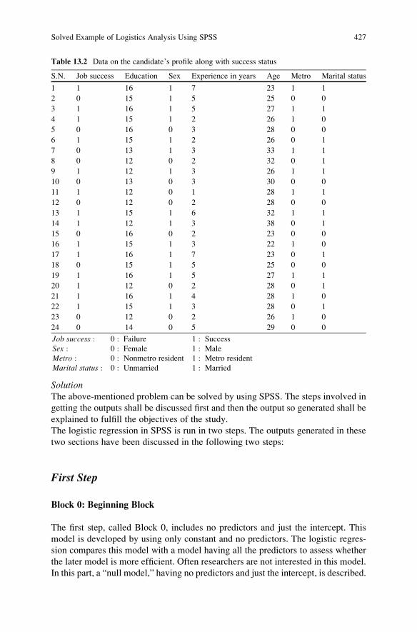
SolutionThe above-mentioned problem can be solved by using SPSS. The steps involved in
getting the outputs shall be discussed first and then the output so generated shall be
explained to fulfill the objectives of the study.
The logistic regression in SPSS is run in two steps. The outputs generated in these
two sections have been discussed in the following two steps:
First Step
Block 0: Beginning Block
The first step, called Block 0, includes no predictors and just the intercept. This
model is developed by using only constant and no predictors. The logistic regres-
sion compares this model with a model having all the predictors to assess whether
the later model is more efficient. Often researchers are not interested in this model.
In this part, a “null model,” having no predictors and just the intercept, is described.
Table 13.2 Data on the candidate’s profile along with success status
S.N. Job success Education Sex Experience in years Age Metro Marital status
1 1 16 1 7 23 1 1
2 0 15 1 5 25 0 0
3 1 16 1 5 27 1 1
4 1 15 1 2 26 1 0
5 0 16 0 3 28 0 0
6 1 15 1 2 26 0 1
7 0 13 1 3 33 1 1
8 0 12 0 2 32 0 1
9 1 12 1 3 26 1 1
10 0 13 0 3 30 0 0
11 1 12 0 1 28 1 1
12 0 12 0 2 28 0 0
13 1 15 1 6 32 1 1
14 1 12 1 3 38 0 1
15 0 16 0 2 23 0 0
16 1 15 1 3 22 1 0
17 1 16 1 7 23 0 1
18 0 15 1 5 25 0 0
19 1 16 1 5 27 1 1
20 1 12 0 2 28 0 1
21 1 16 1 4 28 1 0
22 1 15 1 3 28 0 1
23 0 12 0 2 26 1 0
24 0 14 0 5 29 0 0
Job success : 0 : Failure 1 : Success
Sex : 0 : Female 1 : Male
Metro : 0 : Nonmetro resident 1 : Metro resident
Marital status : 0 : Unmarried 1 : Married
Solved Example of Logistics Analysis Using SPSS 427

Because of this, all the variables entered into the model will figure in the table titled
“Variables not in the Equation.”
Second Step
Block 1: Method ¼ Forward:LR
The second step, called Block 1, includes the information about the variables that
are included and excluded from the analysis, the coding of the dependent variable,
and coding of any categorical variables listed on the categorical subcommand. This
section is the most interesting part of the output in which generated outputs are used
to test the significance of the overall model, regression coefficients, and odds ratios.
The above-mentioned outputs in two steps are generated by the SPSS through a
single sequence of commands, but the outputs are generated in two different
sections with the headings “Block 0: Beginning Block” and “Block 1.” You have
the liberty to use any method of entering independent variables in the model out of
different methods available in SPSS. These will be discussed while explaining
screen shots of logistic regression in the next section.
The procedure of logistic regression in SPSS shall be defined first and then
relevant outputs shall be shown with explanation.
SPSS Commands for the Logistic Regression
To run the commands for logistic regression, a data file is required to be prepared. The
procedure for preparing the data file has been explained inChap. 1. After preparing the
data file, do the following steps for generating outputs in logistic regression:
(i) Data file: In this problem, job success is a dependent variable which is binary in
nature. Out of six independent variables, three variables, namely, sex, metro,
and marital status, are binary, whereas remaining three, education, experience,
and age, are scale variables. In SPSS all binary variables are defined as nominal.
After preparing the data file by defining variable names and their labels, it will
look like as shown in Fig. 13.4.
(ii) Initiating command for logistic regression: After preparing the data file, click
the following commands in sequence (Fig. 13.5):
Analyze ! Regression ! BinaryeLogistic(iii) Selecting variables for analysis: After clicking the Binary Logistic option,
you will get the next screen for selecting dependent and independent variables.
After selecting all the independent variables, you need to select the binary
independent variables included in it by clicking the option. The selection of
variables can be made by following the below-mentioned steps:
428 13 Logistic Regression: Developing a Model for Risk Analysis

– Select the dependent variable from the left panel to the “Dependent” section
in the right panel.
– Select all independent variables including categorical variables from left
panel to the “Covariates” section in the right panel.
– Click the command Categorical and select the categorical variables from
the “Covariates” section to the “Categorical Covariates” in the right panel.
The screen will look like Fig. 13.6.
– Click Continue.
Fig. 13.4 Screen showing data file for the logistic regression analysis in SPSS
Solved Example of Logistics Analysis Using SPSS 429

(iv) Selecting options for computation: After selecting the variables, you need to
define different options for generating the outputs in logistic regression. Do the
following steps:
– Click the tag Options in the screen shown in Fig. 13.6 for selecting outputs
related to statistics and plots. Do the following steps:
– Check “Classification Plots.”
– Check “Hosmer-Lemeshow goodness-of-fit.”
– Let all other default options be selected. The screen will look like Fig. 13.7.
– Click Continue.
(v) Selecting method for entering independent variables in logistic regression: Youneed to define the method of entering the independent variables for developing the
model. You can choose any of the options like Enter, Forward:LR, Forward:Wald,
Backward:LR, orBackward:Wald. Entermethod is usually selectedwhen a specific
model needs to be tested or the contribution of independent variables toward the
target variable is known in advance. On the other hand, if the study is exploratory in
nature, then any of the forward or backward methods can be used. In this study, the
Forward:LR method shall be used because the study is exploratory in nature.
Fig. 13.5 Screen showing of SPSS commands for logistic regression
430 13 Logistic Regression: Developing a Model for Risk Analysis
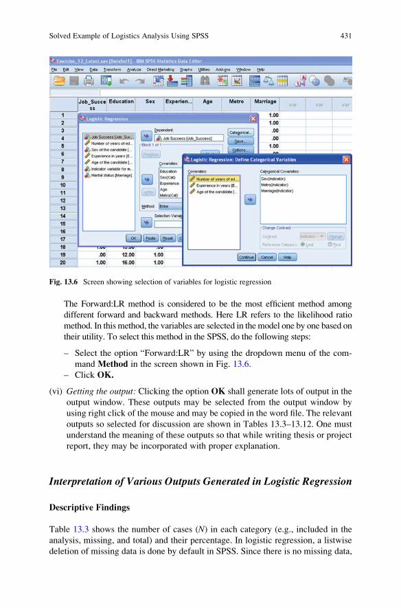
The Forward:LR method is considered to be the most efficient method among
different forward and backward methods. Here LR refers to the likelihood ratio
method. In this method, the variables are selected in the model one by one based on
their utility. To select this method in the SPSS, do the following steps:
– Select the option “Forward:LR” by using the dropdown menu of the com-
mand Method in the screen shown in Fig. 13.6.
– Click OK.
(vi) Getting the output: Clicking the option OK shall generate lots of output in the
output window. These outputs may be selected from the output window by
using right click of the mouse and may be copied in the word file. The relevant
outputs so selected for discussion are shown in Tables 13.3–13.12. One must
understand the meaning of these outputs so that while writing thesis or project
report, they may be incorporated with proper explanation.
Interpretation of Various Outputs Generated in Logistic Regression
Descriptive Findings
Table 13.3 shows the number of cases (N) in each category (e.g., included in the
analysis, missing, and total) and their percentage. In logistic regression, a listwise
deletion of missing data is done by default in SPSS. Since there is no missing data,
Fig. 13.6 Screen showing selection of variables for logistic regression
Solved Example of Logistics Analysis Using SPSS 431

the number of missing cases is shown as 0. Table 13.4 shows the coding of the
dependent variable used in the data file, that is, 1 for success and 0 for failure in
getting the job.
Table 13.5 shows the coding of all the categorical independent variables along
with their frequencies in the study. While coding the categorical variables, highest
number should be allotted to the reference category because by default SPSS
considers the category with the highest coding as the reference category and
gives the code as 0. For instance, if you define the coding of the variable sex as
0 for “female” and 1 for “male,” then the SPSS will consider male as the reference
category and convert its code to 0 and the other category female as 1.
Fig. 13.7 Screen showing option for generating classification plots and Hosmer-Lemeshow
goodness-of-fit
432 13 Logistic Regression: Developing a Model for Risk Analysis
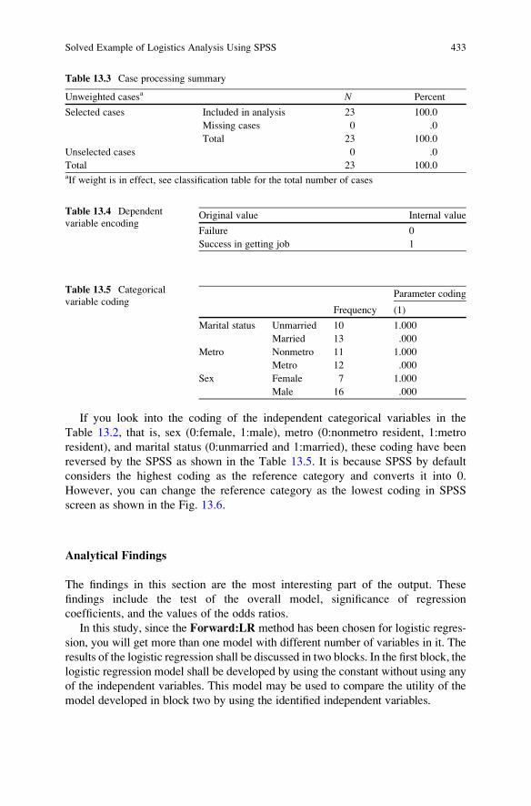
If you look into the coding of the independent categorical variables in the
Table 13.2, that is, sex (0:female, 1:male), metro (0:nonmetro resident, 1:metro
resident), and marital status (0:unmarried and 1:married), these coding have been
reversed by the SPSS as shown in the Table 13.5. It is because SPSS by default
considers the highest coding as the reference category and converts it into 0.
However, you can change the reference category as the lowest coding in SPSS
screen as shown in the Fig. 13.6.
Analytical Findings
The findings in this section are the most interesting part of the output. These
findings include the test of the overall model, significance of regression
coefficients, and the values of the odds ratios.
In this study, since the Forward:LR method has been chosen for logistic regres-
sion, you will get more than one model with different number of variables in it. The
results of the logistic regression shall be discussed in two blocks. In the first block, the
logistic regression model shall be developed by using the constant without using any
of the independent variables. This model may be used to compare the utility of the
model developed in block two by using the identified independent variables.
Table 13.3 Case processing summary
Unweighted casesa N Percent
Selected cases Included in analysis 23 100.0
Missing cases 0 .0
Total 23 100.0
Unselected cases 0 .0
Total 23 100.0aIf weight is in effect, see classification table for the total number of cases
Table 13.4 Dependent
variable encodingOriginal value Internal value
Failure 0
Success in getting job 1
Table 13.5 Categorical
variable codingFrequency
Parameter coding
(1)
Marital status Unmarried 10 1.000
Married 13 .000
Metro Nonmetro 11 1.000
Metro 12 .000
Sex Female 7 1.000
Male 16 .000
Solved Example of Logistics Analysis Using SPSS 433

Block 0: Beginning Block
In Block 0, the results are shown for the model with only the constant included before
any coefficients (i.e., those relating to education, sex, experience, age, metro, and
marital) are entered into the equation. Logistic regression compares the model
obtained in Block 0 with a model including the predictors to determine whether the
latter model is more efficient. The Table 13.6 shows that if nothing is known about
the independent variables and one simple guesses that a person would be selected for
the job, we would be correct 58.3% of the time. Table 13.7 shows that the Wald
statistics is not significant as its significance value is 0.416 which is more than 0.05.
Hence, the model with constant is not worth and is equivalent to just guessing about
the target variable in the absence of any knowledge about the independent variables.
Table 13.8 shows whether each independent variable improves the model or not.
You can see that the variables sex, metro, and marital may improve the model as
they are significant with sex and marital slightly better than metro. Inclusion of
these variables would add to the predictive power of the model. If these variables
had not been significant and able to contribute to the prediction, then the analysis
would obviously be terminated at this stage.
Block 1 Method ¼ Forward:LR
In this block, results of the different models with different independent variables
shall be discussed.
Table 13.9 shows the value of �2 log likelihood (�2LL), which is a deviance
statistic between the observed and predicated values of the dependent variable.
If this deviance statistic is insignificant, it indicates that the model is good and there
is no difference between observed and predicted values of dependent variable. This
number in absolute term is not very informative. However, it can be used to
compare different models having different number of predictive variables. For
Table 13.6 Classification
tablea, bPredicted
Job Percentage correct
Observed Failure Success
Step 0 Job Failure 0 10 0
Success 0 14 100.0
Overall Percentage 58.3aConstant is included in the modelbThe cut value is .500
Table 13.7 Variables
in the equationB S.E. Wald df Sig. Exp(B)
Step 0 Constant .336 .414 .660 1 .416 1.400
434 13 Logistic Regression: Developing a Model for Risk Analysis

instance, in Table 13.9, the value of�2LL has reduced from 24.053 to 18.549. This
indicates that there is an improvement in model 2 by including an additional
variable, sex. In fact, the value of �2LL should keep on decreasing if you go on
adding the significant predictive variables in the model.
Unlike OLS regression equation, there is no concept of R2 in logistic regression.
It is because of the fact that the dependent variable is dichotomous and R2 cannot be
used to show the efficiency of prediction. However, several authors have suggested
pseudo R-squares which are not equivalent to the R-square that is calculated in OLS
regression. Thus, this statistic should be interpreted with great caution. Two such
pseudo R-squares suggested by Cox and Snell and Nagelkerke are shown in
Table 13.9. As per Cox and Snell’s R2, 44.3% of the variation in the dependent
variable is explained by the logistic model. On the other hand, Nagelkerke’s R2
explains 59.7% variability of the dependent variable by the independent variables in
the model. Nagelkerke’s R2 is more reliable measure of relationship in comparison to
Cox and Snell’s R2. Nagelkerke’s R2 will normally be higher than Cox and Snell’s R2.
In order to find whether the deviance statistic �2 log likelihood is insignificant
or not, Hosmer and Lemeshow suggested the chi-square statistic which is shown in
Table 13.10. In order that the model is efficient, this chi-square statistic should be
insignificant. Since the p value associated with chi-square in Table 13.10 is .569 forthe second model, which is greater than .05, it is insignificant and it can be
interpreted that the model is efficient.
Table 13.11 is a classification table which shows the observed and predicted values
of the dependent variable in both themodels. In the secondmodel, it can be seen that out
of 10 candidates who did not get the success in getting the job, four were wrongly
predicted to get the job. Similarly out of 14 candidates who succeeded to get the job,
none was wrongly predicted to be failure. Thus, the model correctly classified 83.3%
cases. This can be obtained by (20/24) � 100.
Table 13.9 Model summary
Step �2 log likelihood Cox and Snell R-square Nagelkerke R-square
1 24.053a .300 .403
2 18.549b .443 .597aEstimation terminated at iteration number 4 because parameter estimates changed by less than
.001bEstimation terminated at iteration number 5 because parameter estimates changed by less than
.001
Table 13.8 Variables not in
the equationScore df Sig.
Step 0 Variables Education 1.073 1 .300
Sex(1) 7.726 1 .005
Experience .728 1 .393
Age .174 1 .677
Metro(1) 4.608 1 .032
Marital(1) 8.061 1 .005
Overall statistics 14.520 6 .024
Solved Example of Logistics Analysis Using SPSS 435

Table 13.12 is the most important table which shows the value of regression
coefficients B, Wald statistics, its significance, and odds ratio exp(B) for each
variable in both the models. The B coefficients are used to develop the logistic
regression equation for predicting the dependent variable from the independent
variables. These coefficients are in log-odds units. Thus, the logistic regression
equation in the second model is given by log p1�p ¼ 2:779� 2:666� Sexð1Þ � 2:7
11�Maritalð1Þwhere p is the probability of getting the job. The dependent variablein the logistic regression is known as logit(p) which is equal to log(p/(1 � p)).
The estimates obtained in the above logistic regression equation explain the
relationship between the independent variables and the dependent variable, where
the dependent variable is on the logit scale. These estimates tell the amount of
increase (or decrease, if the sign of the coefficient is negative) in the estimated log
odds of “job success” ¼ 1 that would be predicted by a 1 unit increase (or decrease)
in the predictor, holding all other predictors constant.
Because regression coefficients B are in log-odds units, they are often difficult to
interpret; hence, they are converted into odds ratios which are equal to exp(B).These odds ratios are shown in the last column of Table 13.12.
Significance of the Wald statistics indicates that the variable significantly
predicts the success in getting the bank job, but it should be used only in a situation
Table 13.10 Hosmer and
Lemeshow testStep Chi-square df Sig.
1 .000 0 .
2 1.129 2 .569
Table 13.11 Classification tablea
Predicted
Job Percentage correct
Observed Failure Success
Step 1 Job Failure 8 2 80.0
Success 3 11 78.6
Overall percentage 79.2
Step 2 Job Failure 6 4 60.0
Success 0 14 100.0
Overall percentage 83.3aThe cut value is .500
Table 13.12 Variables in the
equationB S.E. Wald df Sig. Exp(B)
Step 1a Marital(1) �2.686 1.024 6.874 1 .009 .068
Constant 1.705 .769 4.918 1 .027 5.500
Step 2b Sex(1) �2.666 1.278 4.352 1 .037 .070
Marital(1) �2.711 1.253 4.682 1 .030 .066
Constant 2.779 1.146 5.886 1 .015 16.106aVariable(s) entered on step 1: maritalbVariable(s) entered on step 2: sex
436 13 Logistic Regression: Developing a Model for Risk Analysis

where the sample size is quite large, preferably more than 500. In case of small
sample, the level of significance gets inflated and it does not give the correct
picture. Since in this problem the value of chi-square in Hosmer and Lemeshow
test as shown in Table 13.10 is insignificant, the model can be considered to be valid
for predicting the success in getting the bank’s job on the basis of the second model
with two independent variables, that is, marital and sex.
Explanation of Odds Ratio
In Table 13.12, the exp(B) represents the odds ratio for all the predictors. If the
value of the odds ratio is large, its predictive value is also large. Since the second
model is the final model in this study, the discussion shall be done for the variables
in this model only. Here both the independent variables, that is, sex and marital, are
significant. Since the sex(1) variable has a larger odds ratio .070, this is slightly a
better predictor in comparison to marital(1) variable in getting the bank’s job.
The value of exp(B) for the variable sex(1) is 0.070. It indicates that if the
candidate appearing in the bank exams is female, then there would be decrease in
the odds of 93% (.07–1.00 ¼ �.93). In other words, if a female candidate is
appearing in the bank examination, her chances of success would be 93% less
than the men candidate if other variables are kept constant. Similarly the exp(B)value of the variable marital(1) is .066. This indicates that there would be decrease
in the odds of 93.4% (.066–1.000 ¼ �.934). It can be interpreted that if the
candidate appearing in the bank examination is unmarried, his/her chances of
success would be 93.4% less than the married candidate provided other variables
are kept constant.
Conclusion
To conclude, if the candidate is male and married, the chances of odds increases for
getting selected for a bank job in comparison to female and unmarried candidate.
Summary of the SPSS Commands for Logistic Regression
(i) Start SPSS and prepare the data file by defining the variables and their properties
in Variable View and typing the data column-wise in Data View.
(ii) In the Data View, follow the below-mentioned command sequence for factor
analysis:
Analyze Regression Binary Logistic
Summary of the SPSS Commands for Logistic Regression 437

(iii) Select the dependent variable from the left panel to the “Dependent” section in
the right panel and all independent variables including categorical variables
from left panel to the “Covariates” section in the right panel.
(iv) By clicking the Categorical command, select the categorical variables from
the “Covariates” section to the “Categorical Covariates” in the right panel and
click Continue.(v) Click the tag Options and check “Classification Plots” and “Hosmer-
Lemeshow goodness-of-fit” and click Continue.(vi) Ensure that the option Forward:LR is chosen by default and then clickOK for
output.
Exercise
Short Answer Questions
Note: Write answer to each questions in not more than 200 words.
Q.1. What is logit and how is it used to interpret the probability of success?
Q.2. What do you mean by odds ratio? Explain the monotonic transformation in
relation with odds ratio and log odds.
Q.3. Explain the logistic function and its characteristics.
Q.4. Why is the logit function used in logistic regression analysis?
Q.5. Explain the meaning of maximum likelihood and the significance of �2 log
likelihood.
Q.6. What is the difference between logic regression and OLS regression?
Q.7. How are the dummy variables created in a situation where an independent
categorical variable has more than two options?
Q.8. Write any four assumptions used in logistic regression.
Q.9. What are the advantages of using logistic regression analysis?
Q.10. Explain any one research situation in detail where logistic regression can be
applied.
Q.11. Write in brief the various steps involved in logistic regression.
Q.12. What is Hosmer and Lemeshow test? How is it used and what does it indicate?
Multiple-Choice Questions
Note: For each of the question, there are four alternative answers for each question.
Tick mark the one that you consider the closest to the correct answer.
1. Logistic regression is used when the dependent variable is
(a) Continuous
(b) Ordinal
(c) Binary
(d) Categorical
2. If exp(3) ¼ 20.12, then log(20.12) is
(a) 20.12
(b) 23.12
438 13 Logistic Regression: Developing a Model for Risk Analysis

(c) 17.12
(d) 3
3. If the probability of success is 0.6, then the odds of success is
(a) 0.4
(b) 1.5
(c) 2.4
(d) 0.75
4. In a logistic regression, if the odds ratio for an independent variable is 2.5, then
which of the following is true?
(a) The probability of the dependent variable happening is 0.25.
(b) The odds against the dependent variable happening is 2.5.
(c) The odds for the dependent variable happening is 2.5.
(d) The odds for the dependent variable happening is 2.5 against one unit
increase in the independent variable.
5. If p is the probability of success, then the logit of p is
(a) ln 1�pp
(b) ln 1þpp
(c) log p1�p
(d) log p1þp
6. The logistic function f(z) is equal to
(a) eZ
1þeZ
(b) 1þeZ
eZ
(c) eZ
1�eZ
(d) 1�eZ
eZ
7. In logistic regression, odds ratio is equivalent to
(a) Log(B)(b) Exp(B)(c) B coefficient
(d) p1�p
8. Choose the correct statement.
(a) The independent variable is required to be linearly related with the depen-
dent variable.
(b) The independent variable is required to be linearly related with logit
transformation of the outcome variable.
(c) The dependent variable is always continuous.
(d) Probability of success in the outcome variable is equivalent to the log odds.
Exercise 439

9. Choose the correct command for starting logistic regression in SPSS.
(a) Analyze ! Regression ! Binary Logistic
(b) Analyze ! Regression ! Logistic Regression
(c) Analyze ! Binary Logistic ! Regression
(d) Analyze ! Logistic ! Binary Regression
10. In using the Hosmer-Lemeshow goodness-of-fit, model is considered to be
good if
(a) Chi-square is significant at any predefined level.
(b) Chi-square is not significant at any predefined level.
(c) Chi-square is equal to 100.
(d) All the regression coefficients are significant.
Assignments
1. Following are the scores of 90 candidates in different subjects obtained in a
MBA entrance examination. Apply the logistic regression to develop a model for
predicting success in the examination on the basis of independent variables.
Discuss the comparative importance of independent variables in predicting
success in the examination. For the variable MBA, coding 1 represents success
and 0 indicates failure in the examination. Similarly gender 1 indicates male and
2 indicates female.
MBA English Reasoning Math Gender MBA English Reasoning Math Gender
1 68 50 65 0 0 46 52 55 1
0 39 44 52 1 0 39 41 33 0
0 44 44 46 1 0 52 49 49 0
1 50 54 61 1 0 28 46 43 0
1 71 65 72 0 0 42 54 50 1
1 63 65 71 1 0 47 42 52 0
0 34 44 40 0 0 47 57 48 1
1 63 49 69 0 0 52 59 58 0
0 68 43 64 0 0 47 52 43 1
0 47 45 56 1 1 55 62 41 0
0 47 46 49 1 0 44 52 43 0
0 63 52 54 0 0 47 41 46 0
0 52 51 53 0 0 45 55 44 1
0 55 54 66 0 0 47 37 43 0
1 60 68 67 1 0 65 54 61 0
0 35 35 40 0 0 43 57 40 1
0 47 54 46 1 0 47 54 49 0
1 71 63 69 0 1 57 62 56 0
0 57 52 40 1 0 68 59 61 1
0 44 50 41 0 0 52 55 50 0
0 65 46 57 0 0 42 57 51 0
1 68 59 58 1 0 42 39 42 1
(continued)
440 13 Logistic Regression: Developing a Model for Risk Analysis
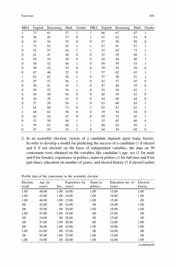
MBA English Reasoning Math Gender MBA English Reasoning Math Gender
1 73 61 57 1 1 66 67 67 1
0 36 44 37 0 1 47 62 53 0
0 43 54 55 0 0 57 50 50 0
1 73 62 62 1 1 47 61 51 1
0 52 57 64 1 1 57 62 72 1
0 41 47 40 0 0 52 59 48 1
0 50 54 50 0 0 44 44 40 1
0 50 52 46 1 0 50 59 53 1
0 50 52 53 0 0 39 54 39 0
0 47 46 52 0 1 57 62 63 1
1 62 62 45 1 0 57 50 51 1
0 55 57 56 1 0 42 57 45 0
0 50 41 45 1 0 47 46 39 0
0 39 53 54 1 0 42 36 42 1
0 50 49 56 0 0 60 59 62 0
0 34 35 41 0 0 44 49 44 0
0 57 59 54 1 0 63 60 65 1
1 65 60 72 0 1 65 67 63 1
1 68 62 56 0 0 39 54 54 0
0 42 54 47 0 0 50 52 45 1
0 53 59 49 1 1 52 65 60 0
1 59 63 60 1 1 60 62 49 1
0 47 59 54 1 0 44 49 48 0
2. In an assembly election, victory of a candidate depends upon many factors.
In order to develop a model for predicting the success of a candidate (1 if elected
and 0 if not elected) on the basis of independent variables, the data on 30
contestants were obtained on the variables like candidate’s age, sex (1 for male
and 0 for female), experience in politics, status in politics (1 for full time and 0 for
part time), education (in number of years), and elected history (1 if elected earlier
Profile data of the contestants in the assembly election
Election
result
Age (in
years) Sex
Experience (in
years)
Status in
politics
Education (no. of
years)
Election
history
1.00 48.00 1.00 10.00 1.00 15.00 1.00
1.00 42.00 1.00 16.00 1.00 18.00 1.00
1.00 46.00 1.00 12.00 1.00 15.00 .00
.00 42.00 .00 16.00 .00 16.00 1.00
.00 45.00 .00 20.00 1.00 18.00 1.00
1.00 47.00 1.00 18.00 .00 15.00 .00
.00 34.00 .00 28.00 .00 15.00 .00
.00 47.00 1.00 20.00 .00 12.00 1.00
.00 36.00 1.00 30.00 1.00 10.00 1.00
1.00 63.00 .00 35.00 .00 16.00 .00
.00 45.00 1.00 25.00 1.00 12.00 .00
1.00 54.00 .00 20.00 1.00 16.00 1.00
(continued)
Exercise 441

and 0 if not elected earlier). Apply the logistic regression and develop the model
for predicting success in assembly election.
Answers to Multiple-Choice Questions
Q.1 c Q.2 d Q.3 b Q.4 d
Q.5 c Q.6 a Q.7 b Q.8 b
Q.9 a Q.10 b
Election
result
Age (in
years) Sex
Experience (in
years)
Status in
politics
Education (no. of
years)
Election
history
1.00 58.00 1.00 34.00 .00 18.00 .00
.00 54.00 .00 38.00 .00 12.00 .00
.00 56.00 1.00 35.00 .00 10.00 1.00
1.00 55.00 .00 30.00 1.00 15.00 .00
1.00 54.00 .00 31.00 1.00 16.00 .00
1.00 58.00 1.00 34.00 .00 15.00 1.00
.00 37.00 1.00 35.00 .00 10.00 .00
1.00 45.00 1.00 22.00 .00 15.00 1.00
.00 34.00 1.00 5.00 1.00 12.00 1.00
.00 47.00 .00 9.00 .00 12.00 1.00
.00 42.00 1.00 8.00 .00 12.00 1.00
1.00 45.00 1.00 6.00 .00 15.00 .00
1.00 28.00 1.00 2.00 1.00 16.00 1.00
1.00 43.00 .00 12.00 1.00 16.00 1.00
.00 35.00 1.00 11.00 1.00 15.00 1.00
1.00 43.00 .00 18.00 1.00 15.00 .00
1.00 45.00 .00 17.00 .00 16.00 1.00
1.00 41.00 1.00 13.00 .00 15.00 1.00
.00 42.00 1.00 15.00 1.00 15.00 .00
442 13 Logistic Regression: Developing a Model for Risk Analysis

Chapter 14
Multidimensional Scaling for Product
Positioning
Learning Objectives
After completing this chapter, you should be able to do the following:
• Know the use of multidimensional scaling in market research.
• Understand the different terms used in multidimensional scaling.
• Learn the procedures used in multidimensional scaling.
• Able to identify the research situations where multidimensional scaling can be
used.
• Describe the SPSS procedure involved in multidimensional scaling.
• Explain the various outputs generated by the SPSS in this analysis.
Introduction
Multidimensional scaling (MDS) is a series of statistical techniques used for
identifying the key dimensions underlying respondents’ evaluations of objects
and keeping them in multidimensional space. MDS is widely used in marketing
research for positioning of brands. It would be desired for any company to know as
to how its brand of products is rated among other similar competing brands. While
assessing the brand image of any product, the respondents may rate it on the basis of
its overall image or on the basis of certain attributes. Thus, besides knowing the
relative positioning of the products, one may like to know the strength of the
product in comparison to other similar products on different dimensions. The
MDS can be used to solve varieties of problems in management research. For
example, it finds application in market segmentation, product life cycle, vendor
evaluation, and advertising media selection.
Though it is possible to use MDS with quantitative variables (i.e., on the basis of
price, aesthetics, color, size, shape, weight, etc.), but it is mostly used to compare
objects in a situation where the bases of comparison are not known. This approach
of the MDS is a philosophical perspective because every person experiences the
J.P. Verma, Data Analysis in Management with SPSS Software,DOI 10.1007/978-81-322-0786-3_14, # Springer India 2013
443
world in their own way. From this perspective, MDS procedure based on the
predefined attributes is not completely satisfactory as it fails to take the individual
experience into account. One way to overcome this problem is to look at the
constructs an individual use to construe the world. Since the MDS is often used
to identify key dimensions underlying customer evaluations of products, services,
or companies, therefore once the data is at hand, multidimensional scaling can help
determine the following:
• While evaluating the objects, what dimensions are used by the respondents?
• The relative importance of each dimension.
• How the objects are placed in the perceptual map.
Thus, by using the multidimensional scaling methods, one can analyze their
current level of consumer satisfaction in the market and modify the marketing mix
based upon the current consumer preference and satisfaction.
What Is Multidimensional Scaling
Multidimensional scaling is a sequence of techniques for exploring similarities or
preferences among objects. These objects can be products, organizations, brands,
outlets, etc. In this technique, similarities or preferences of objects are measured on
some dimensions, and accordingly the objects are positioned in the multidimen-
sional space for understanding the brand positioning. Through multidimensional
technique, a researcher can get an idea about the respondent’s perceived relative
image of a set of objects. The multidimensional scaling is also known as perceptual
mapping. In this technique, we transform consumer judgments of overall similarity
or preferences into distances represented in multidimensional space.
Terminologies Used in Multidimensional Scaling
Objects and Subjects
In multidimensional scaling, the object refers to the products, organizations,
opinions, or other choices to be compared and positioned in multidimensional
space. The objects are also known as variables or stimuli. On the other hand, the
subject refers to the respondents who rate the objects in multidimensional scaling.
The subjects are the one who are picked up in the sample for conducting the
research study. Sometimes the subjects are termed as the “source,” and the objects
are termed as “target.”
444 14 Multidimensional Scaling for Product Positioning

Distances
Distance refers to the difference in the two objects on any one or more dimension as
perceived by a respondent. It is the fundamental measurement concept in MDS.
Distance may also be referred as similarity, preferences, dissimilarity, or proximity.
There exist many alternative distance measures, but all are functions of dissimilar-
ity/similarity or preference judgments.
Similarity vs. Dissimilarity Matrices
If the cells of matrix represent the degree of similarity between pairs represented by
the rows and columns of the matrix, then the matrix is said to be similarity matrix.
On the other hand, if cells of the matrix represent the extent to which one object is
preferred over other in the pair, then the matrix is said to be dissimilarity matrix.
Larger cell values represent greater distance. The algorithm used by SPSS in
multidimensional scaling is more efficient with dissimilarity/preference measures
than with similarity/proximity measures. For this reason, distance matrices are used
in SPSS instead of similarity matrices.
Stress
Stress (phi) is a goodness-of-fit test that measures the efficiency of the MDS
models. The smaller the stress, the better is the fit. Stress measures the difference
between interpoint distances in computed MDS space and the corresponding actual
input distances. High stress indicates measurement error, and also it may reflect
having too few dimensions. Stress is not much affected by sample size provided the
number of objects is appreciably more than the number of dimensions.
Perceptual Mapping
Perceptual mapping is a graphical representation of objects in multidimensional
space. In perceptual map, points are shown for both, that is, column as well as row
objects. In obtaining the perceptual map, the consumer’s views about a product are
plotted on a chart. Respondents are asked to give their preferences by showing each
of the pair of the objects by asking about their experience with the product in terms
of its performance, packaging, price, size, etc. These qualitative responses are
shown on a chart (called a perceptual map) using a suitable scale (such as the
Likert scale). The results of the perceptual mapping are used in improving the
product or developing a new product.
Terminologies Used in Multidimensional Scaling 445
Dimensions
While preparing dissimilarity matrix, the respondent may be asked to rate the two
objects/products on a particular characteristics such as color, look, energy effi-
ciency, and cost. These characteristics are said to be the dimension on which the
evaluation may take place. Usually the products are rated on two or more than two
dimensions. These dimensions may be predefined or may be perceived by the
respondents of their own.
What We Do in Multidimensional Scaling?
The multidimensional scaling technique can be applied by either using
dissimilarity-based approach or attribute-based approach. The methodologies
adopted in these two approaches shall be discussed in detail below. However,
solved example shall be discussed only for dissimilarity-based approach of multi-
dimensional scaling. The detail working of this approach with SPSS has been
shown in Example 14.1.
Procedure of Dissimilarity-Based Approach of MultidimensionalScaling
The dissimilarity-based approach is very simple to understand and is very useful in
understanding the consumer behavior. In this approach, the respondents are asked
to rate different pairs of comparable objects on the basis of their experience. While
evaluating the pair of objects, the dissimilarity measure is noted on the basis of
some of the parameters that the respondents have in their mind. No predefined
attributes or objective criteria are given on the basis of which the respondent can
evaluate the two objects in the pair. Following steps are adopted in this approach:
Steps in Dissimilarity-Based Approach
1. Find the distance matrix among all the objects. It can be obtained by simply
ranking of distances between an object and all other objects by a consumer. This
matrix can be obtained by providing the consumer a card containing pair of
objects written on it, and the candidate needs to specify a number indicating the
difference between the two objects on any numerical scale which can represent
distance between the two objects. This process is repeated for all pairs of brands
being included in the study. In this process, no attributes are identified on which
the consumer is asked to decide on the difference. The distance measure so
446 14 Multidimensional Scaling for Product Positioning
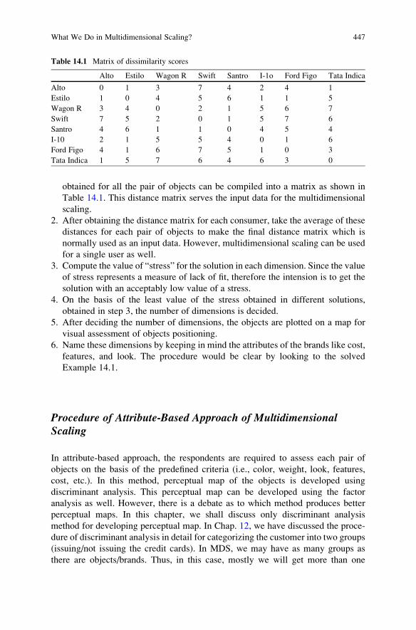
obtained for all the pair of objects can be compiled into a matrix as shown in
Table 14.1. This distance matrix serves the input data for the multidimensional
scaling.
2. After obtaining the distance matrix for each consumer, take the average of these
distances for each pair of objects to make the final distance matrix which is
normally used as an input data. However, multidimensional scaling can be used
for a single user as well.
3. Compute the value of “stress” for the solution in each dimension. Since the value
of stress represents a measure of lack of fit, therefore the intension is to get the
solution with an acceptably low value of a stress.
4. On the basis of the least value of the stress obtained in different solutions,
obtained in step 3, the number of dimensions is decided.
5. After deciding the number of dimensions, the objects are plotted on a map for
visual assessment of objects positioning.
6. Name these dimensions by keeping in mind the attributes of the brands like cost,
features, and look. The procedure would be clear by looking to the solved
Example 14.1.
Procedure of Attribute-Based Approach of MultidimensionalScaling
In attribute-based approach, the respondents are required to assess each pair of
objects on the basis of the predefined criteria (i.e., color, weight, look, features,
cost, etc.). In this method, perceptual map of the objects is developed using
discriminant analysis. This perceptual map can be developed using the factor
analysis as well. However, there is a debate as to which method produces better
perceptual maps. In this chapter, we shall discuss only discriminant analysis
method for developing perceptual map. In Chap. 12, we have discussed the proce-
dure of discriminant analysis in detail for categorizing the customer into two groups
(issuing/not issuing the credit cards). In MDS, we may have as many groups as
there are objects/brands. Thus, in this case, mostly we will get more than one
Table 14.1 Matrix of dissimilarity scores
Alto Estilo Wagon R Swift Santro I-1o Ford Figo Tata Indica
Alto 0 1 3 7 4 2 4 1
Estilo 1 0 4 5 6 1 1 5
Wagon R 3 4 0 2 1 5 6 7
Swift 7 5 2 0 1 5 7 6
Santro 4 6 1 1 0 4 5 4
I-10 2 1 5 5 4 0 1 6
Ford Figo 4 1 6 7 5 1 0 3
Tata Indica 1 5 7 6 4 6 3 0
What We Do in Multidimensional Scaling? 447

discriminant function. For example, in case of three objects/brands, you could get
two functions, and with four objects, you may get up to three discriminant
functions. The solution of discriminant analysis gives the value of eigenvalue for
each discriminant function. This eigenvalue explains the amount of variance that is
explained by the discriminant function. This percentage variance explained by the
discriminant function is used to decide as to how many discriminant functions one
should use. If two discriminant functions are used, then they form two axes of the
perceptual map. Whereas if three discriminant functions are used, then you get
three perceptual maps, that is, function 1 vs. function 2, function 1 vs. function 3,
and function 2 vs. function 3. These discriminant functions represent the axes on
which the objects are first located and thereafter the attributes are located.
To find the number of dimensions and the perceptual map of different objects,
following steps are used:
1. Obtain consumers’ perceptions on different attributes on the different competing
brands. This serves as the input data for the discriminant analysis.
2. Run the discriminant analysis by taking all the independent variables together in
the model. The option for this method can be seen in SPSS as “Enter
independents together.”
3. The SPSS output shall generate the following results:
(a) Group statistics including mean and standard deviation
(b) Unstandardized canonical discriminant function coefficients table
(c) Eigen values and canonical correlation
(d) Wilks’ lambda and chi-square test
(e) Classification matrix
(f) Standardized canonical discriminant function coefficients
(g) Functions at group centroids
Remark: For generating the above-mentioned outputs for MDS, you can refer
back the solved Example 12.1 in Chap. 12.
4. The eigenvalue would decide as to how many discriminant function you want to
use.
5. Draw perceptual map (or maps) separately by using the standardized canonical
discriminant coefficients. This can be done by using Excel or any other graphic
package. The discriminant function denotes the axes on which the objects/brands
are first located, and then attributes are placed on the same graph.
Assumptions in Multidimensional Scaling
Following assumptions are made while performing the multidimensional scaling:
1. All respondents will rate the objects on the same dimensions.
2. Dimensions are orthogonal.
448 14 Multidimensional Scaling for Product Positioning

3. The respondents have the same perception about the dimensionality in assessing
the distances among the objects.
4. Respondents will attach the same level of importance to a dimension, even if all
respondents perceive this dimension.
5. There is no change in the judgments of a stimulus in terms of either dimensions
or levels of importance over time.
Limitations of Multidimensional Scaling
Although MDS is widely used for positioning the brand image and comparing the
product characteristics, it has some limitations as well.
1. It is difficult to obtain the similarity and preferences of the respondents toward a
group of objects because perceptions of the subjects may differ considerably.
2. Because every product has lots of variant model having different characteristics
and therefore the group of objects taken for comparing their brand image may
itself differ on many counts. Due to this fact, true positioning may not be
possible.
3. Preferences change over time, place, and socioeconomic status and therefore
brand positioning obtained in a particular study may not be generalized.
4. The bias exists in the data collection.
5. In case of nonmetric data, all the MDS techniques are subject to the problem of
local optima and degenerate solutions.
6. Although metric MDS are more robust than nonmetric MDS and produce good
maps but the dimension interpretation, the main work of MDS is highly subjec-
tive and depends upon the questioning of the interviewers.
Solved Example of Multidimensional Scaling (Dissimilarity-
Based Approach of Multidimensional Scaling) Using SPSS
Example 14.1 Twenty customers were asked to rate 8 cars by showing the cards
bearing the name of a pair of cars. All possible pair of cars were shown, and the
customers were asked to rate their preferences of one car over other on an 8-point
scale. If the customer perceived that the two cars were completely dissimilar, a
score of 8 was given, and if the two cars were exactly similar, a score of 0 was
given. Following dissimilarity scores were obtained and are shown in Table 14.1.
Use multidimensional scaling to find the number of dimensions the consumers use
in assessing different brands and name these dimensions. Develop perceptual map
and position these eight brands of cars in a multidimensional space.
Solved Example of Multidimensional Scaling . . . 449

Solution In order to find the number of dimensions used by the consumers in
assessing these eight brands of car, the multidimensional scaling option of SPSS
shall be used to generate outputs showing stress value for the solutions of different
dimensions. Simultaneously dimensions for stimulus coordinates in different
solutions shall also be obtained which shall be used to place all the eight brands
of cars in the multidimensional map.
SPSS Commands for Multidimensional Scaling
The data file needs to be prepared before using SPSS commands to generate outputs
in multidimensional scaling. Following steps would be performed to get the rele-
vant outputs for further interpretation in the analysis.
(i) Data file: Here, eight variables need to be defined. All these variables shall be
defined as ordinal as the scores are the dissimilarity ratings. After preparing the
data file by defining variable names and their labels, it will look like Fig. 14.1.
(ii) Initiating command for multidimensional analysis: After preparing the data
file, click the following command sequence in the Data View:
Analyze ! Scale ! Multidimensional Scaling (ALSCAL)
The screen shall look like Fig. 14.2.
(iii) Selecting variables for discriminant analysis: After clicking the Multidimen-
sional Scaling option, the SPSS will take you to the window where variables
are selected.
• Select all the variables from left panel to the “Variables” section of the right
panel.
• Click the tag Model in the screen shown in Fig. 14.3.
– Write minimum and maximum dimension for which the solution is
required. Since, in this problem, there are eight brands, hence maximum
of up to three-dimensional solution shall be obtained. In case of more
number of brands, solutions of more dimensions may be investigated.
– Let other options are checked by default.
– Click Continue.
• Click the tag Option in the screen as shown in screen 14.3.
– Check the option “Group plots” in the Display section.
– Let other options are checked by default.
– Click Continue.
The screen for these options shall look like Fig. 14.4.
– Click OK for output.
450 14 Multidimensional Scaling for Product Positioning

(iv) Getting the output: After clicking the OK option in Fig. 14.3, the output in the
multidimensional scaling shall be generated in the output window. Selected
outputs can be copied in the word file by using the right click of the mouse over
identified area of the output. Out of many outputs generated by the SPSS, the
following relevant outputs have been picked up for discussion:
Fig. 14.1 Screen showing data file for the multidimensional scaling in SPSS
Fig. 14.2 Screen showing SPSS commands for multidimensional scaling
Solved Example of Multidimensional Scaling . . . 451
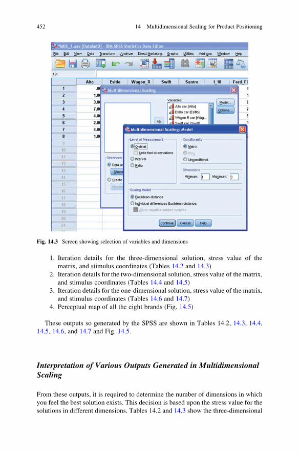
1. Iteration details for the three-dimensional solution, stress value of the
matrix, and stimulus coordinates (Tables 14.2 and 14.3)
2. Iteration details for the two-dimensional solution, stress value of the matrix,
and stimulus coordinates (Tables 14.4 and 14.5)
3. Iteration details for the one-dimensional solution, stress value of the matrix,
and stimulus coordinates (Tables 14.6 and 14.7)
4. Perceptual map of all the eight brands (Fig. 14.5)
These outputs so generated by the SPSS are shown in Tables 14.2, 14.3, 14.4,
14.5, 14.6, and 14.7 and Fig. 14.5.
Interpretation of Various Outputs Generated in MultidimensionalScaling
From these outputs, it is required to determine the number of dimensions in which
you feel the best solution exists. This decision is based upon the stress value for the
solutions in different dimensions. Tables 14.2 and 14.3 show the three-dimensional
Fig. 14.3 Screen showing selection of variables and dimensions
452 14 Multidimensional Scaling for Product Positioning

solution, and the stress value for these solutions is 0.07911. Tables 14.4 and 14.5
contain two-dimensional solutions along with the stress value as 0.16611. On the
other hand, the one-dimensional solutions are shown in Tables 14.6 and 14.7 along
with the stress value 0.42024.
Stress value shows the lack of fit, and therefore, it should be as close to zero as
possible. Owing to these criteria, the one-dimensional solution is not good at all as
this contains the maximum value of stress (0.42024). The two-dimensional solution
looks better as it is close to zero, but the three-dimensional solution is the best
because its stress value is the least.
Since in this problem there are only eight brands, therefore it is not possible to
get a solution in more than three dimensions. If you have more than 14 or 15 brands,
you may try some higher dimension solution. To find out the optimum solution, one
needs to have the trade-off between stress value and the number of dimensions.
Three-Dimensional Solution
Based on the stress value, the three-dimensional solution is the best as in that case
the stress value is the least and closest to zero. Therefore, the next task is to define
Fig. 14.4 Screen showing the options for perceptual mapping
Solved Example of Multidimensional Scaling . . . 453
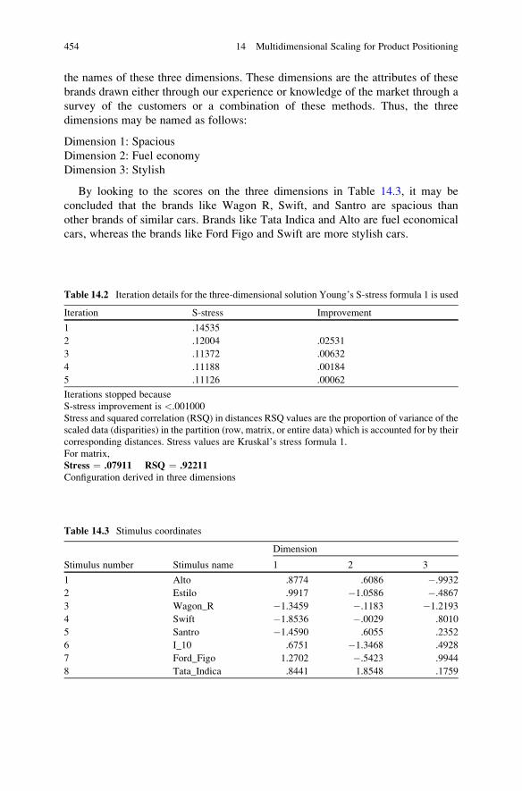
the names of these three dimensions. These dimensions are the attributes of these
brands drawn either through our experience or knowledge of the market through a
survey of the customers or a combination of these methods. Thus, the three
dimensions may be named as follows:
Dimension 1: Spacious
Dimension 2: Fuel economy
Dimension 3: Stylish
By looking to the scores on the three dimensions in Table 14.3, it may be
concluded that the brands like Wagon R, Swift, and Santro are spacious than
other brands of similar cars. Brands like Tata Indica and Alto are fuel economical
cars, whereas the brands like Ford Figo and Swift are more stylish cars.
Table 14.2 Iteration details for the three-dimensional solution Young’s S-stress formula 1 is used
Iteration S-stress Improvement
1 .14535
2 .12004 .02531
3 .11372 .00632
4 .11188 .00184
5 .11126 .00062
Iterations stopped because
S-stress improvement is <.001000
Stress and squared correlation (RSQ) in distances RSQ values are the proportion of variance of the
scaled data (disparities) in the partition (row, matrix, or entire data) which is accounted for by their
corresponding distances. Stress values are Kruskal’s stress formula 1.
For matrix,
Stress ¼ .07911 RSQ ¼ .92211
Configuration derived in three dimensions
Table 14.3 Stimulus coordinates
Stimulus number Stimulus name
Dimension
1 2 3
1 Alto .8774 .6086 �.9932
2 Estilo .9917 �1.0586 �.4867
3 Wagon_R �1.3459 �.1183 �1.2193
4 Swift �1.8536 �.0029 .8010
5 Santro �1.4590 .6055 .2352
6 I_10 .6751 �1.3468 .4928
7 Ford_Figo 1.2702 �.5423 .9944
8 Tata_Indica .8441 1.8548 .1759
454 14 Multidimensional Scaling for Product Positioning
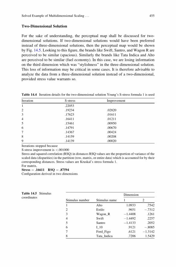
Two-Dimensional Solution
For the sake of understanding, the perceptual map shall be discussed for two-
dimensional solutions. If two-dimensional solutions would have been preferred
instead of three-dimensional solutions, then the perceptual map would be shown
by Fig. 14.5. Looking to this figure, the brands like Swift, Santro, and Wagon R are
perceived to be similar (spacious). Similarly the brands like Tata Indica and Alto
are perceived to be similar (fuel economy). In this case, we are losing information
on the third dimension which was “stylishness” in the three-dimensional solution.
This loss of information may be critical in some cases. It is therefore advisable to
analyze the data from a three-dimensional solution instead of a two-dimensional,
provided stress value warrants so.
Table 14.4 Iteration details for the two-dimensional solution Young’s S-stress formula 1 is used
Iteration S-stress Improvement
1 .22053
2 .19234 .02820
3 .17623 .01611
4 .16411 .01211
5 .15461 .00950
6 .14791 .00670
7 .14367 .00424
8 .14159 .00208
9 .14139 .00020
Iterations stopped because
S-stress improvement is <.001000
Stress and squared correlation (RSQ) in distances RSQ values are the proportion of variance of the
scaled data (disparities) in the partition (row, matrix, or entire data) which is accounted for by their
corresponding distances. Stress values are Kruskal’s stress formula 1.
For matrix,
Stress ¼ .16611 RSQ ¼ .87594
Configuration derived in two dimensions
Table 14.5 Stimulus
coordinatesStimulus number Stimulus name
Dimension
1 2
1 Alto 1.0933 .7542
2 Estilo .9651 �.7312
3 Wagon_R �1.4408 .1261
4 Swift �1.4492 .2257
5 Santro �1.4133 .2052
6 I_10 .9121 �.8085
7 Ford_Figo .6121 �1.3142
8 Tata_Indica .7206 1.5429
Solved Example of Multidimensional Scaling . . . 455

Table 14.6 Iteration details for the one-dimensional solution Young’s S-stress formula 1 is used
Iteration S-stress Improvement
1 .44444
2 .43243 .01201
3 .43185 .00057
Iterations stopped because
S-stress improvement is <.001000
Stress and squared correlation (RSQ) in distances RSQ values are the proportion of variance of the
scaled data (disparities) in the partition (row, matrix, or entire data) which is accounted for by their
corresponding distances. Stress values are Kruskal’s stress formula 1.
For matrix,
Stress ¼ .42024 RSQ ¼ .57334
Configuration derived in one dimension
Fig. 14.5 Perceptual map of different brands of car (two-dimensional output)
Table 14.7 Stimulus
coordinatesStimulus number Stimulus name
Dimension
1
1 Alto �.8034
2 Estilo �.7738
3 Wagon_R 1.2367
4 Swift 1.4484
5 Santro 1.1694
6 I_10 �.6166
7 Ford_Figo �.8593
8 Tata_Indica �.8015
Summary of the SPSS Commands for Multidimensional Scaling
(i) Start SPSS and prepare the data file by defining the variables and their
properties in Variable View and typing the data column wise in Data View.
(ii) In the data view, follow the below-mentioned command sequence for multidi-
mensional scaling:
Analyze ! Scale ! Multidimensional Scaling (ALSCAL)
(iii) Select all the variables from left panel to the “Variables” section of the right
panel.
(iv) Click the tagModel and write minimum and maximum dimension for which the
solution is required. Let other options are checked by default. Click Continue.(v) Click the tag Option in the screen and check the option “Group plots” in the
Display section. Let other options are checked by default. Click Continue.Click OK for output.
Exercise
Short Answer Questions
Note: Write answer to each of the following questions in not more than 200 words.
1. Define multidimensional scaling and explain a situation in marketing where
this technique can be used.
2. Discuss the procedure used in dissimilarity-based approach of multidimen-
sional scaling.
3. What are the steps used in attribute-based approach of multidimensional
scaling?
4. What are the drawbacks of multidimensional scaling?
5. Explain the assumptions used in multidimensional scaling.
6. Describe any five terminologies used in multidimensional scaling.
7. What do you mean by stress score? What is its significance and how is it used in
deciding the solution in multidimensional scaling?
8. What are the various considerations in deciding the name of the dimensions?
9. What do you mean by a perceptual map? Explain by means of an example.
10. Explain the difference in attribute-based approach and dissimilarity-based
approach of multidimensional scaling.
Multiple-Choice Questions
Note: Question no. 1–10 has four alternative answers for each question. Tick mark
the one that you consider the closest to the correct answer.
Exercise 457

1. MDS refers to
(a) Multidimensional spaces
(b) Multidirectional spaces
(c) Multidimensional perceptual scaling
(d) Multidimensional scaling
2. Stress is a measure of
(a) Distance between the two brands
(b) Goodness of fit
(c) Correctness of the perceptual map
(d) Error involved in deciding the nomenclature of dimensions
3. Perceptual mapping is a
(a) Graphical representation of the dimensions in multidimensional space
(b) Graphical representation of objects in multidimensional space
(c) Graphical representation of the distances of the objects
(d) Graphical representation of brands in two-dimensional space
4. Dimensions refer to
(a) The brands on which clustering is made
(b) The characteristics of the brands which are clubbed for assessment
(c) The brands which have some attributes common in them
(d) The characteristics on which the evaluation may take place
5. In dissimilarity-based approach of multidimensional scaling, the input data are
(a) Nominal
(b) Ordinal
(c) Scale
(d) Ratio
6. The solution of multidimensional is accurate if the value of stress is
(a) Less than 1
(b) More than 1
(c) Closer to 0
(d) Closer to 0.5
7. In attribute-based approach of multidimensional scaling, the input data can be
(a) Interval
(b) Nominal
(c) Ordinal
(d) None of the above
8. One of the assumptions in multidimensional scaling is
(a) The respondents will not rate the objects on the same dimensions.
(b) Dimensions are orthogonal.
458 14 Multidimensional Scaling for Product Positioning

(c) Respondents will not attach the same level of importance to a dimension,
even if all respondents perceive this dimension.
(d) Data are nominal.
9. Choose the correct sequence of commands in SPSS for multidimensional scaling.
(a) Analyze ! Scale ! Multidimensional Scaling (ALSCAL)
(b) Analyze ! Multidimensional Scaling (ALSCAL) ! Scale
(c) Analyze ! Scale ! Multidimensional Scaling (PROXSCAL)
(d) Analyze ! Multidimensional Scaling (PROXSCAL) ! Scale
10. Following solutions are obtained in the multidimensional scaling:
(i) One-Dimensional Solution with Stress score ¼ 0.7659
(ii) Two-Dimensional Solution with Stress score ¼ 0.4328
(iii) Three-Dimensional Solution with Stress score ¼ 0.1348
(iv) Four-Dimensional Solution with Stress score ¼ 0.0924
Which solution would you prefer?
(a) ii
(b) i
(c) iv
(d) iii
Assignments
1. A refrigerator company wanted to draw a perceptual map using its consumers’
perceptions regarding its own brand and five competing brands. These six brands
were Samsung, LG, Videocon, Godrej, Sharp, and Hitachi. The customers were
shown a card containing a pair of names of these brands and were asked to rate in
terms of dissimilarity between the two on an 8-point rating scale. The rating of
8 indicates that the two brands are distinctively apart, whereas 1 indicates that the
two brands are exactly similar as perceived by the customers. This exercise was
done on all the pair of brands. The average dissimilarity ratings obtained by all the
customers are shown in the following table. Apply the multidimensional scaling
and interpret your findings by plotting the perceptual map of these brands.
2. The authorities in a university wanted to assess its teachers as perceived by their
students on a seven-point scale by drawing the perceptual map. Six teachers,
Dissimilarity ratings obtained by the customers on the six brands of the refrigerators
Samsung LG Videocon Godrej Sharp Hitachi
Samsung 0 4 3 7 4 3
LG 0 3 8 3 2
Videocon 0 7 3 5
Godrej 0 6 8
Sharp 0 4
Hitachi 0
Exercise 459

Smith, Anderson, Clark, Wright, Mitchell and Johnson were rated by 25 students.
Score 7 indicated that the two teachers were distinctively apart, whereas the
score 1 represented that they were exactly similar as perceived by the students.
Following is the dissimilarity matrix obtained on the basis of the average
dissimilarity scores obtained on all the 25 students. By using the multidimen-
sional scaling technique, draw the perceptual map.
Answers of Multiple-Choice Questions
Q.1 d Q.2 b Q.3 b Q.4 d
Q.5 b Q.6 c Q.7 a Q.8 b
Q.9 a Q.10 d
Dissimilarity ratings obtained by the students on the teachers in the college
Smith Anderson Clark Wright Mitchell Johnson
Smith 0 4 3 1 5 6
Anderson 3 2 5 3 2
Clark 0 4 3 4
Wright 0 6 5
Mitchell 0 4
Johnson 0
460 14 Multidimensional Scaling for Product Positioning

Appendix: Tables
Table A.1 The normal curve area between the mean and a given z value
Z 0.00 0.01 0.02 0.03 0.04 0.05 0.06 0.07 0.08 0.09
0.0 0.0000 0.0040 0.0080 0.0120 0.0160 0.0199 0.0239 0.0279 0.0319 0.0359
0.1 0.0398 0.0438 0.0478 0.0517 0.0557 0.0596 0.0636 0.0675 0.0714 0.0753
0.2 0.0793 0.0832 0.0871 0.0910 0.0948 0.0987 0.1026 0.1064 0.1103 0.1141
0.3 0.1179 0.1217 0.1255 0.1293 0.1331 0.1368 0.1406 0.1443 0.1480 0.1517
0.4 0.1554 0.1591 0.1628 0.1664 0.1700 0.1736 0.1772 0.1808 0.1844 0.1879
0.5 0.1915 0.1950 0.1985 0.2019 0.2054 0.2088 0.2123 0.2157 0.2190 0.2224
0.6 0.2257 0.2291 0.2324 0.2357 0.2389 0.2422 0.2454 0.2486 0.2517 0.2549
0.7 0.2580 0.2611 0.2642 0.2673 0.2704 0.2734 0.2764 0.2794 0.2823 0.2852
0.8 0.2881 0.2910 0.2939 0.2967 0.2995 0.3023 0.3051 0.3078 0.3106 0.3133
0.9 0.3159 0.3186 0.3212 0.3238 0.3264 0.3289 0.3315 0.3340 0.3365 0.3389
1.0 0.3413 0.3438 0.3461 0.3485 0.3508 0.3531 0.3554 0.3577 0.3599 0.3621
1.1 0.3643 0.3665 0.3686 0.3708 0.3729 0.3749 0.3770 0.3790 0.3810 0.3830
1.2 0.3849 0.3869 0.3888 0.3907 0.3925 0.3944 0.3962 0.3980 0.3997 0.4015
1.3 0.4032 0.4049 0.4066 0.4082 0.4099 0.4115 0.4131 0.4147 0.4162 0.4177
1.4 0.4192 0.4207 0.4222 0.4236 0.4251 0.4265 0.4279 0.4292 0.4306 0.4319
1.5 0.4332 0.4345 0.4357 0.4370 0.4382 0.4394 0.4406 0.4418 0.4429 0.4441
1.6 0.4452 0.4463 0.4474 0.4484 0.4495 0.4505 0.4515 0.4525 0.4535 0.4545
1.7 0.4554 0.4564 0.4573 0.4582 0.4591 0.4599 0.4608 0.4616 0.4625 0.4633
1.8 0.4641 0.4649 0.4656 0.4664 0.4671 0.4678 0.4686 0.4693 0.4699 0.4706
1.9 0.4713 0.4719 0.4726 0.4732 0.4738 0.4744 0.4750 0.4756 0.4761 0.4767
2.0 0.4772 0.4778 0.4783 0.4788 0.4793 0.4798 0.4803 0.4808 0.4812 0.4817
2.1 0.4821 0.4826 0.4830 0.4834 0.4838 0.4842 0.4846 0.4850 0.4854 0.4857
2.2 0.4861 0.4864 0.4868 0.4871 0.4875 0.4878 0.4881 0.4884 0.4887 0.4890
2.3 0.4893 0.4896 0.4898 0.4901 0.4904 0.4906 0.4909 0.4911 0.4913 0.4916
2.4 0.4918 0.4920 0.4922 0.4925 0.4927 0.4929 0.4931 0.4932 0.4934 0.4936
2.5 0.4938 0.4940 0.4941 0.4943 0.4945 0.4946 0.4948 0.4949 0.4951 0.4952
2.6 0.4953 0.4955 0.4956 0.4957 0.4959 0.4960 0.4961 0.4962 0.4963 0.4964
2.7 0.4965 0.4966 0.4967 0.4968 0.4969 0.4970 0.4971 0.4972 0.4973 0.4974
2.8 0.4974 0.4975 0.4976 0.4977 0.4977 0.4978 0.4979 0.4979 0.4980 0.4981
2.9 0.4981 0.4982 0.4982 0.4983 0.4984 0.4984 0.4985 0.4985 0.4986 0.4986
3.0 0.4987 0.4987 0.4987 0.4988 0.4988 0.4989 0.4989 0.4989 0.4990 0.4990
J.P. Verma, Data Analysis in Management with SPSS Software,DOI 10.1007/978-81-322-0786-3, # Springer India 2013
461

Table A.2 Critical values of ‘t’
Level of significance (a)
one-tail 0.50 0.25 0.20 0.15 0.10 0.05 0.025 0.01 0.005 0.001 0.0005
two-tail df 1.00 0.50 0.40 0.30 0.20 0.10 0.05 0.02 0.01 0.002 0.001
1 0.000 1.000 1.376 1.963 3.078 6.314 12.71 31.82 63.66 318.31 636.62
2 0.000 0.816 1.061 1.386 1.886 2.920 4.303 6.965 9.925 22.327 31.599
3 0.000 0.765 0.978 1.250 1.638 2.353 3.182 4.541 5.841 10.215 12.924
4 0.000 0.741 0.941 1.190 1.533 2.132 2.776 3.747 4.604 7.173 8.610
5 0.000 0.727 0.920 1.156 1.476 2.015 2.571 3.365 4.032 5.893 6.869
6 0.000 0.718 0.906 1.134 1.440 1.943 2.447 3.143 3.707 5.208 5.959
7 0.000 0.711 0.896 1.119 1.415 1.895 2.365 2.998 3.499 4.785 5.408
8 0.000 0.706 0.889 1.108 1.397 1.860 2.306 2.896 3.355 4.501 5.041
9 0.000 0.703 0.883 1.100 1.383 1.833 2.262 2.821 3.250 4.297 4.781
10 0.000 0.700 0.879 1.093 1.372 1.812 2.228 2.764 3.169 4.144 4.587
11 0.000 0.697 0.876 1.088 1.363 1.796 2.201 2.718 3.106 4.025 4.437
12 0.000 0.695 0.873 1.083 1.356 1.782 2.179 2.681 3.055 3.930 4.318
13 0.000 0.694 0.870 1.079 1.350 1.771 2.160 2.650 3.012 3.852 4.221
14 0.000 0.692 0.868 1.076 1.345 1.761 2.145 2.624 2.977 3.787 4.140
15 0.000 0.691 0.866 1.074 1.341 1.753 2.131 2.602 2.947 3.733 4.073
16 0.000 0.690 0.865 1.071 1.337 1.746 2.120 2.583 2.921 3.686 4.015
17 0.000 0.689 0.863 1.069 1.333 1.740 2.110 2.567 2.898 3.646 3.965
18 0.000 0.688 0.862 1.067 1.330 1.734 2.101 2.552 2.878 3.610 3.922
19 0.000 0.688 0.861 1.066 1.328 1.729 2.093 2.539 2.861 3.579 3.883
20 0.000 0.687 0.860 1.064 1.325 1.725 2.086 2.528 2.845 3.552 3.850
21 0.000 0.686 0.859 1.063 1.323 1.721 2.080 2.518 2.831 3.527 3.819
22 0.000 0.686 0.858 1.061 1.321 1.717 2.074 2.508 2.819 3.505 3.792
23 0.000 0.685 0.858 1.060 1.319 1.714 2.069 2.500 2.807 3.485 3.768
24 0.000 0.685 0.857 1.059 1.318 1.711 2.064 2.492 2.797 3.467 3.745
25 0.000 0.684 0.856 1.058 1.316 1.708 2.060 2.485 2.787 3.450 3.725
26 0.000 0.684 0.856 1.058 1.315 1.706 2.056 2.479 2.779 3.435 3.707
27 0.000 0.684 0.855 1.057 1.314 1.703 2.052 2.473 2.771 3.421 3.690
28 0.000 0.683 0.855 1.056 1.313 1.701 2.048 2.467 2.763 3.408 3.674
29 0.000 0.683 0.854 1.055 1.311 1.699 2.045 2.462 2.756 3.396 3.659
30 0.000 0.683 0.854 1.055 1.310 1.697 2.042 2.457 2.750 3.385 3.646
40 0.000 0.681 0.851 1.050 1.303 1.684 2.021 2.423 2.704 3.307 3.551
60 0.000 0.679 0.848 1.045 1.296 1.671 2.000 2.390 2.660 3.232 3.460
80 0.000 0.678 0.846 1.043 1.292 1.664 1.990 2.374 2.639 3.195 3.416
100 0.000 0.677 0.845 1.042 1.290 1.660 1.984 2.364 2.626 3.174 3.390
1,000 0.000 0.675 0.842 1.037 1.282 1.646 1.962 2.330 2.581 3.098 3.300
1 0.000 0.674 0.842 1.036 1.282 1.645 1.960 2.326 2.576 3.090 3.291
462 Appendix: Tables

Table A.3 Critical values of
the correlation coefficientLevel of significance for two-tailed test
df (n�2) 0.10 0.05 0.02 0.01
1 0.988 0.997 0.9995 0.9999
2 0.900 0.950 0.980 0.990
3 0.805 0.878 0.934 0.959
4 0.729 0.811 0.882 0.917
5 0.669 0.754 0.833 0.874
6 0.622 0.707 0.789 0.834
7 0.582 0.666 0.750 0.798
8 0.549 0.632 0.716 0.765
9 0.521 0.602 0.685 0.735
10 0.497 0.576 0.658 0.708
11 0.476 0.553 0.634 0.684
12 0.458 0.532 0.612 0.661
13 0.441 0.514 0.592 0.641
14 0.426 0.497 0.574 0.623
15 0.412 0.482 0.558 0.606
16 0.400 0.468 0.542 0.590
17 0.389 0.456 0.528 0.575
18 0.378 0.444 0.516 0.561
19 0.369 0.433 0.503 0.549
20 0.360 0.423 0.492 0.537
21 0.352 0.413 0.482 0.526
22 0.344 0.404 0.472 0.515
23 0.337 0.396 0.462 0.505
24 0.330 0.388 0.453 0.496
25 0.323 0.381 0.445 0.487
26 0.317 0.374 0.437 0.479
27 0.311 0.367 0.430 0.471
28 0.306 0.361 0.423 0.463
29 0.301 0.355 0.416 0.456
30 0.296 0.349 0.409 0.449
35 0.275 0.325 0.381 0.418
40 0.257 0.304 0.358 0.393
45 0.243 0.288 0.338 0.372
50 0.231 0.273 0.322 0.354
60 0.211 0.250 0.295 0.325
70 0.195 0.232 0.274 0.303
80 0.183 0.217 0.256 0.283
90 0.173 0.205 0.242 0.267
100 0.164 0.195 0.230 0.254
df (n�2) 0.05 0.25 0.01 0.005
Level of significance for one tailed test
Appendix: Tables 463

Table A.4 F-table: critical values at .05 level of significance
n1=n2 1 2 3 4 5 6 7 8 9 10 11 12 13 14 15 16 17 18 19
3 10.13 9.55 9.28 9.12 9.01 8.94 8.89 8.85 8.81 8.79 8.76 8.74 8.73 8.71 8.70 8.69 8.68 8.67 8.67
4 7.71 6.94 6.59 6.39 6.26 6.16 6.09 6.04 6.00 5.96 5.94 5.91 5.89 5.87 5.86 5.84 5.83 5.82 5.81
5 6.61 5.79 5.41 5.19 5.05 4.95 4.88 4.82 4.77 4.74 4.70 4.68 4.66 4.64 4.62 4.60 4.59 4.58 4.57
6 5.99 5.14 4.76 4.53 4.39 4.28 4.21 4.15 4.10 4.06 4.03 4.00 3.98 3.96 3.94 3.92 3.91 3.90 3.88
7 5.59 4.74 4.35 4.12 3.97 3.87 3.79 3.73 3.68 3.64 3.60 3.57 3.55 3.53 3.51 3.49 3.48 3.47 3.46
8 5.32 4.46 4.07 3.84 3.69 3.58 3.50 3.44 3.39 3.35 3.31 3.28 3.26 3.24 3.22 3.20 3.19 3.17 3.16
9 5.12 4.26 3.86 3.63 3.48 3.37 3.29 3.23 3.18 3.14 3.10 3.07 3.05 3.03 3.01 2.99 2.97 2.96 2.95
10 4.96 4.10 3.71 3.48 3.33 3.22 3.14 3.07 3.02 2.98 2.94 2.91 2.89 2.86 2.85 2.83 2.81 2.80 2.79
11 4.84 3.98 3.59 3.36 3.20 3.09 3.01 2.95 2.90 2.85 2.82 2.79 2.76 2.74 2.72 2.70 2.69 2.67 2.66
12 4.75 3.89 3.49 3.26 3.11 3.00 2.91 2.85 2.80 2.75 2.72 2.69 2.66 2.64 2.62 2.60 2.58 2.57 2.56
13 4.67 3.81 3.41 3.18 3.03 2.92 2.83 2.77 2.71 2.67 2.63 2.60 2.58 2.55 2.53 2.51 2.50 2.48 2.47
14 4.60 3.74 3.34 3.11 2.96 2.85 2.76 2.70 2.65 2.60 2.57 2.53 2.51 2.48 2.46 2.44 2.43 2.41 2.40
15 4.54 3.68 3.29 3.06 2.90 2.79 2.71 2.64 2.59 2.54 2.51 2.48 2.45 2.42 2.40 2.38 2.37 2.35 2.34
16 4.49 3.63 3.24 3.01 2.85 2.74 2.66 2.59 2.54 2.49 2.46 2.42 2.40 2.37 2.35 2.33 2.32 2.30 2.29
17 4.45 3.59 3.20 2.96 2.81 2.70 2.61 2.55 2.49 2.45 2.41 2.38 2.35 2.33 2.31 2.29 2.27 2.26 2.24
18 4.41 3.55 3.16 2.93 2.77 2.66 2.58 2.51 2.46 2.41 2.37 2.34 2.31 2.29 2.27 2.25 2.23 2.22 2.20
19 4.38 3.52 3.13 2.90 2.74 2.63 2.54 2.48 2.42 2.38 2.34 2.31 2.28 2.26 2.23 2.21 2.20 2.18 2.17
20 4.35 3.49 3.10 2.87 2.71 2.60 2.51 2.45 2.39 2.35 2.31 2.28 2.25 2.23 2.20 2.18 2.17 2.15 2.14
22 4.30 3.44 3.05 2.82 2.66 2.55 2.46 2.40 2.34 2.30 2.26 2.23 2.20 2.17 2.15 2.13 2.11 2.10 2.08
24 4.26 3.40 3.01 2.78 2.62 2.51 2.42 2.36 2.30 2.25 2.22 2.18 2.15 2.13 2.11 2.09 2.07 2.05 2.04
26 4.23 3.37 2.98 2.74 2.59 2.47 2.39 2.32 2.27 2.22 2.18 2.15 2.12 2.09 2.07 2.05 2.03 2.02 2.00
28 4.20 3.34 2.95 2.71 2.56 2.45 2.36 2.29 2.24 2.19 2.15 2.12 2.09 2.06 2.04 2.02 2.00 1.99 1.97
30 4.17 3.32 2.92 2.69 2.53 2.42 2.33 2.27 2.21 2.16 2.13 2.09 2.06 2.04 2.01 1.99 1.98 1.96 1.95
35 4.12 3.27 2.87 2.64 2.49 2.37 2.29 2.22 2.16 2.11 2.08 2.04 2.01 1.99 1.96 1.94 1.92 1.91 1.89
40 4.08 3.23 2.84 2.61 2.45 2.34 2.25 2.18 2.12 2.08 2.04 2.00 1.97 1.95 1.92 1.90 1.89 1.87 1.85
45 4.06 3.20 2.81 2.58 2.42 2.31 2.22 2.15 2.10 2.05 2.01 1.97 1.94 1.92 1.89 1.87 1.86 1.84 1.82
50 4.03 3.18 2.79 2.56 2.40 2.29 2.20 2.13 2.07 2.03 1.99 1.95 1.92 1.89 1.87 1.85 1.83 1.81 1.80
60 4.00 3.15 2.76 2.53 2.37 2.25 2.17 2.10 2.04 1.99 1.95 1.92 1.89 1.86 1.84 1.82 1.80 1.78 1.76
70 3.98 3.13 2.74 2.50 2.35 2.23 2.14 2.07 2.02 1.97 1.93 1.89 1.86 1.84 1.81 1.79 1.77 1.75 1.74
80 3.96 3.11 2.72 2.49 2.33 2.21 2.13 2.06 2.00 1.95 1.91 1.88 1.84 1.82 1.79 1.77 1.75 1.73 1.72
100 3.94 3.09 2.70 2.46 2.31 2.19 2.10 2.03 1.97 1.93 1.89 1.85 1.82 1.79 1.77 1.75 1.73 1.71 1.69
200 3.89 3.04 2.65 2.42 2.26 2.14 2.06 1.98 1.93 1.88 1.84 1.80 1.77 1.74 1.72 1.69 1.67 1.66 1.64
500 3.86 3.01 2.62 2.39 2.23 2.12 2.03 1.96 1.90 1.85 1.81 1.77 1.74 1.71 1.69 1.66 1.64 1.62 1.61
1,000 3.85 3.00 2.61 2.38 2.22 2.11 2.02 1.95 1.89 1.84 1.80 1.76 1.73 1.70 1.68 1.65 1.63 1.61 1.60
>1,000 1.04 3.00 2.61 2.37 2.21 2.10 2.01 1.94 1.88 1.83 1.79 1.75 1.72 1.69 1.67 1.64 1.62 1.61 1.59
n1/n2 1 2 3 4 5 6 7 8 9 10 11 12 13 14 15 16 17 18 19
464 Appendix: Tables

20 22 24 26 28 30 35 40 45 50 60 70 80 100 200 500 1,000 >1,000 n1/n2
8.66 8.65 8.64 8.63 8.62 8.62 8.60 8.59 8.59 8.58 8.57 8.57 8.56 8.55 8.54 8.53 8.53 8.54 3
5.80 5.79 5.77 5.76 5.75 5.75 5.73 5.72 5.71 5.70 5.69 5.68 5.67 5.66 5.65 5.64 5.63 5.63 4
4.56 4.54 4.53 4.52 4.50 4.50 4.48 4.46 4.45 4.44 4.43 4.42 4.42 4.41 4.39 4.37 4.37 4.36 5
3.87 3.86 3.84 3.83 3.82 3.81 3.79 3.77 3.76 3.75 3.74 3.73 3.72 3.71 3.69 3.68 3.67 3.67 6
3.44 3.43 3.41 3.40 3.39 3.38 3.36 3.34 3.33 3.32 3.30 3.29 3.29 3.27 3.25 3.24 3.23 3.23 7
3.15 3.13 3.12 3.10 3.09 3.08 3.06 3.04 3.03 3.02 3.01 2.99 2.99 2.97 2.95 2.94 2.93 2.93 8
2.94 2.92 2.90 2.89 2.87 2.86 2.84 2.83 2.81 2.80 2.79 2.78 2.77 2.76 2.73 2.72 2.71 2.71 9
2.77 2.75 2.74 2.72 2.71 2.70 2.68 2.66 2.65 2.64 2.62 2.61 2.60 2.59 2.56 2.55 2.54 2.54 10
2.65 2.63 2.61 2.59 2.58 2.57 2.55 2.53 2.52 2.51 2.49 2.48 2.47 2.46 2.43 2.42 2.41 2.41 11
2.54 2.52 2.51 2.49 2.48 2.47 2.44 2.43 2.41 2.40 2.38 2.37 2.36 2.35 2.32 2.31 2.30 2.30 12
2.46 2.44 2.42 2.41 2.39 2.38 2.36 2.34 2.33 2.31 2.30 2.28 2.27 2.26 2.23 2.22 2.21 2.21 13
2.39 2.37 2.35 2.33 2.32 2.31 2.28 2.27 2.25 2.24 2.22 2.21 2.20 2.19 2.16 2.14 2.14 2.13 14
2.33 2.31 2.29 2.27 2.26 2.25 2.22 2.20 2.19 2.18 2.16 2.15 2.14 2.12 2.10 2.08 2.07 2.07 15
2.28 2.25 2.24 2.22 2.21 2.19 2.17 2.15 2.14 2.12 2.11 2.09 2.08 2.07 2.04 2.02 2.02 2.01 16
2.23 2.21 2.19 2.17 2.16 2.15 2.12 2.10 2.09 2.08 2.06 2.05 2.03 2.02 1.99 1.97 1.97 1.96 17
2.19 2.17 2.15 2.13 2.12 2.11 2.08 2.06 2.05 2.04 2.02 2.00 1.99 1.98 1.95 1.93 1.92 1.92 18
2.16 2.13 2.11 2.10 2.08 2.07 2.05 2.03 2.01 2.00 1.98 1.97 1.96 1.94 1.91 1.89 1.88 1.88 19
2.12 2.10 2.08 2.07 2.05 2.04 2.01 1.99 1.98 1.97 1.95 1.93 1.92 1.91 1.88 1.86 1.85 1.84 20
2.07 2.05 2.03 2.01 2.00 1.98 1.96 1.94 1.92 1.91 1.89 1.88 1.86 1.85 1.82 1.80 1.79 1.78 22
2.03 2.00 1.98 1.97 1.95 1.94 1.91 1.89 1.88 1.86 1.84 1.83 1.82 1.80 1.77 1.75 1.74 1.73 24
1.99 1.97 1.95 1.93 1.91 1.90 1.87 1.85 1.84 1.82 1.80 1.79 1.78 1.76 1.73 1.71 1.70 1.69 26
1.96 1.93 1.91 1.90 1.88 1.87 1.84 1.82 1.80 1.79 1.77 1.75 1.74 1.73 1.69 1.67 1.66 1.66 28
1.93 1.91 1.89 1.87 1.85 1.84 1.81 1.79 1.77 1.76 1.74 1.72 1.71 1.70 1.66 1.64 1.63 1.62 30
1.88 1.85 1.83 1.82 1.80 1.79 1.76 1.74 1.72 1.70 1.68 1.66 1.65 1.63 1.60 1.57 1.57 1.56 35
1.84 1.81 1.79 1.77 1.76 1.74 1.72 1.69 1.67 1.66 1.64 1.62 1.61 1.59 1.55 1.53 1.52 1.51 40
1.81 1.78 1.76 1.74 1.73 1.71 1.68 1.66 1.64 1.63 1.60 1.59 1.57 1.55 1.51 1.49 1.48 1.47 45
1.78 1.76 1.74 1.72 1.70 1.69 1.66 1.63 1.61 1.60 1.58 1.56 1.54 1.52 1.48 1.46 1.45 1.44 50
1.75 1.72 1.70 1.68 1.66 1.65 1.62 1.59 1.57 1.56 1.53 1.52 1.50 1.48 1.44 1.41 1.40 1.39 60
1.72 1.70 1.67 1.65 1.64 1.62 1.59 1.57 1.55 1.53 1.50 1.49 1.47 1.45 1.40 1.37 1.36 1.35 70
1.70 1.68 1.65 1.63 1.62 1.60 1.57 1.54 1.52 1.51 1.48 1.46 1.45 1.43 1.38 1.35 1.34 1.33 80
1.68 1.65 1.63 1.61 1.59 1.57 1.54 1.52 1.49 1.48 1.45 1.43 1.41 1.39 1.34 1.31 1.30 1.28 100
1.62 1.60 1.57 1.55 1.53 1.52 1.48 1.46 1.43 1.41 1.39 1.36 1.35 1.32 1.26 1.22 1.21 1.19 200
1.59 1.56 1.54 1.52 1.50 1.48 1.45 1.42 1.40 1.38 1.35 1.32 1.30 1.28 1.21 1.16 1.14 1.12 500
1.58 1.55 1.53 1.51 1.49 1.47 1.43 1.41 1.38 1.36 1.33 1.31 1.29 1.26 1.19 1.13 1.11 1.08 1,000
1.57 1.54 1.52 1.50 1.48 1.46 1.42 1.40 1.37 1.35 1.32 1.30 1.28 1.25 1.17 1.11 1.08 1.03 >1,000
20 22 24 26 28 30 35 40 45 50 60 70 80 100 200 500 1,000 >1,000 n1/n2
Appendix: Tables 465

Table A.5 F-table: critical values at .01 level of significance
n1/n2 1 2 3 4 5 6 7 8 9 10 11 12 13 14 15 16 17 18
3 34.12 30.82 29.46 28.71 28.24 27.91 27.67 27.49 27.35 27.23 27.13 27.05 26.98 26.92 26.87 26.83 26.79 26.75
4 21.20 18.00 16.69 15.98 15.52 15.21 14.98 14.80 14.66 14.55 14.45 14.37 14.31 14.25 14.20 14.15 14.11 14.08
5 16.26 13.27 12.06 11.39 10.97 10.67 10.46 10.29 10.16 10.05 9.96 9.89 9.82 9.77 9.72 9.68 9.64 9.61
6 13.75 10.92 9.78 9.15 8.75 8.47 8.26 8.10 7.98 7.87 7.79 7.72 7.66 7.61 7.56 7.52 7.48 7.45
7 12.25 9.55 8.45 7.85 7.46 7.19 6.99 6.84 6.72 6.62 6.54 6.47 6.41 6.36 6.31 6.28 6.24 6.21
8 11.26 8.65 7.59 7.01 6.63 6.37 6.18 6.03 5.91 5.81 5.73 5.67 5.61 5.56 5.52 5.48 5.44 5.41
9 10.56 8.02 6.99 6.42 6.06 5.80 5.61 5.47 5.35 5.26 5.18 5.11 5.05 5.01 4.96 4.92 4.89 4.86
10 10.04 7.56 6.55 5.99 5.64 5.39 5.20 5.06 4.94 4.85 4.77 4.71 4.65 4.60 4.56 4.52 4.49 4.46
11 9.65 7.21 6.22 5.67 5.32 5.07 4.89 4.74 4.63 4.54 4.46 4.40 4.34 4.29 4.25 4.21 4.18 4.15
12 9.33 6.93 5.95 5.41 5.06 4.82 4.64 4.50 4.39 4.30 4.22 4.16 4.10 4.05 4.01 3.97 3.94 3.91
13 9.07 6.70 5.74 5.21 4.86 4.62 4.44 4.30 4.19 4.10 4.02 3.96 3.91 3.86 3.82 3.78 3.75 3.72
14 8.86 6.51 5.56 5.04 4.70 4.46 4.28 4.14 4.03 3.94 3.86 3.80 3.75 3.70 3.66 3.62 3.59 3.56
15 8.68 6.36 5.42 4.89 4.56 4.32 4.14 4.00 3.89 3.80 3.73 3.67 3.61 3.56 3.52 3.49 3.45 3.42
16 8.53 6.23 5.29 4.77 4.44 4.20 4.03 3.89 3.78 3.69 3.62 3.55 3.50 3.45 3.41 3.37 3.34 3.31
17 8.40 6.11 5.19 4.67 4.34 4.10 3.93 3.79 3.68 3.59 3.52 3.46 3.40 3.35 3.31 3.27 3.24 3.21
18 8.29 6.01 5.09 4.58 4.25 4.01 3.84 3.71 3.60 3.51 3.43 3.37 3.32 3.27 3.23 3.19 3.16 3.13
19 8.19 5.93 5.01 4.50 4.17 3.94 3.77 3.63 3.52 3.43 3.36 3.30 3.24 3.19 3.15 3.12 3.08 3.05
20 8.10 5.85 4.94 4.43 4.10 3.87 3.70 3.56 3.46 3.37 3.29 3.23 3.18 3.13 3.09 3.05 3.02 2.99
22 7.95 5.72 4.82 4.31 3.99 3.76 3.59 3.45 3.35 3.26 3.18 3.12 3.07 3.02 2.98 2.94 2.91 2.88
24 7.82 5.61 4.72 4.22 3.90 3.67 3.50 3.36 3.26 3.17 3.09 3.03 2.98 2.93 2.89 2.85 2.82 2.79
26 7.72 5.53 4.64 4.14 3.82 3.59 3.42 3.29 3.18 3.09 3.02 2.96 2.90 2.86 2.82 2.78 2.75 2.72
28 7.64 5.45 4.57 4.07 3.75 3.53 3.36 3.23 3.12 3.03 2.96 2.90 2.84 2.79 2.75 2.72 2.68 2.65
30 7.56 5.39 4.51 4.02 3.70 3.47 3.30 3.17 3.07 2.98 2.91 2.84 2.79 2.74 2.70 2.66 2.63 2.60
35 7.42 5.27 4.40 3.91 3.59 3.37 3.20 3.07 2.96 2.88 2.80 2.74 2.69 2.64 2.60 2.56 2.53 2.50
40 7.31 5.18 4.31 3.83 3.51 3.29 3.12 2.99 2.89 2.80 2.73 2.66 2.61 2.56 2.52 2.48 2.45 2.42
45 7.23 5.11 4.25 3.77 3.45 3.23 3.07 2.94 2.83 2.74 2.67 2.61 2.55 2.51 2.46 2.43 2.39 2.36
50 7.17 5.06 4.20 3.72 3.41 3.19 3.02 2.89 2.79 2.70 2.63 2.56 2.51 2.46 2.42 2.38 2.35 2.32
60 7.08 4.98 4.13 3.65 3.34 3.12 2.95 2.82 2.72 2.63 2.56 2.50 2.44 2.39 2.35 2.31 2.28 2.25
70 7.01 4.92 4.07 3.60 3.29 3.07 2.91 2.78 2.67 2.59 2.51 2.45 2.40 2.35 2.31 2.27 2.23 2.20
80 6.96 4.88 4.04 3.56 3.26 3.04 2.87 2.74 2.64 2.55 2.48 2.42 2.36 2.31 2.27 2.23 2.20 2.17
100 6.90 4.82 3.98 3.51 3.21 2.99 2.82 2.69 2.59 2.50 2.43 2.37 2.31 2.27 2.22 2.19 2.15 2.12
200 6.76 4.71 3.88 3.41 3.11 2.89 2.73 2.60 2.50 2.41 2.34 2.27 2.22 2.17 2.13 2.09 2.06 2.03
500 6.69 4.65 3.82 3.36 3.05 2.84 2.68 2.55 2.44 2.36 2.28 2.22 2.17 2.12 2.07 2.04 2.00 1.97
1,000 6.66 4.63 3.80 3.34 3.04 2.82 2.66 2.53 2.43 2.34 2.27 2.20 2.15 2.10 2.06 2.02 1.98 1.95
>1,000 1.04 4.61 3.78 3.32 3.02 2.80 2.64 2.51 2.41 2.32 2.25 2.19 2.13 2.08 2.04 2.00 1.97 1.94
n1/n2 1 2 3 4 5 6 7 8 9 10 11 12 13 14 15 16 17 18
466 Appendix: Tables

19 20 22 24 26 28 30 35 40 45 50 60 70 80 100 200 500 1,000 >1,000 n1/n2
26.72 26.69 26.64 26.60 26.56 26.53 26.50 26.45 26.41 26.38 26.35 26.32 26.29 26.27 26.24 26.18 26.15 26.13 26.15 3
14.05 14.02 13.97 13.93 13.89 13.86 13.84 13.79 13.75 13.71 13.69 13.65 13.63 13.61 13.58 13.52 13.49 13.47 13.47 4
9.58 9.55 9.51 9.47 9.43 9.40 9.38 9.33 9.29 9.26 9.24 9.20 9.18 9.16 9.13 9.08 9.04 9.03 9.02 5
7.42 7.40 7.35 7.31 7.28 7.25 7.23 7.18 7.14 7.11 7.09 7.06 7.03 7.01 6.99 6.93 6.90 6.89 6.89 6
6.18 6.16 6.11 6.07 6.04 6.02 5.99 5.94 5.91 5.88 5.86 5.82 5.80 5.78 5.75 5.70 5.67 5.66 5.65 7
5.38 5.36 5.32 5.28 5.25 5.22 5.20 5.15 5.12 5.09 5.07 5.03 5.01 4.99 4.96 4.91 4.88 4.87 4.86 8
4.83 4.81 4.77 4.73 4.70 4.67 4.65 4.60 4.57 4.54 4.52 4.48 4.46 4.44 4.42 4.36 4.33 4.32 4.32 9
4.43 4.41 4.36 4.33 4.30 4.27 4.25 4.20 4.17 4.14 4.12 4.08 4.06 4.04 4.01 3.96 3.93 3.92 3.91 10
4.12 4.10 4.06 4.02 3.99 3.96 3.94 3.89 3.86 3.83 3.81 3.78 3.75 3.73 3.71 3.66 3.62 3.61 3.60 11
3.88 3.86 3.82 3.78 3.75 3.72 3.70 3.65 3.62 3.59 3.57 3.54 3.51 3.49 3.47 3.41 3.38 3.37 3.36 12
3.69 3.66 3.62 3.59 3.56 3.53 3.51 3.46 3.43 3.40 3.38 3.34 3.32 3.30 3.27 3.22 3.19 3.18 3.17 13
3.53 3.51 3.46 3.43 3.40 3.37 3.35 3.30 3.27 3.24 3.22 3.18 3.16 3.14 3.11 3.06 3.03 3.01 3.01 14
3.40 3.37 3.33 3.29 3.26 3.24 3.21 3.17 3.13 3.10 3.08 3.05 3.02 3.00 2.98 2.92 2.89 2.88 2.87 15
3.28 3.26 3.22 3.18 3.15 3.12 3.10 3.05 3.02 2.99 2.97 2.93 2.91 2.89 2.86 2.81 2.78 2.76 2.75 16
3.19 3.16 3.12 3.08 3.05 3.03 3.00 2.96 2.92 2.89 2.87 2.83 2.81 2.79 2.76 2.71 2.68 2.66 2.65 17
3.10 3.08 3.03 3.00 2.97 2.94 2.92 2.87 2.84 2.81 2.78 2.75 2.72 2.71 2.68 2.62 2.59 2.58 2.57 18
3.03 3.00 2.96 2.92 2.89 2.87 2.84 2.80 2.76 2.73 2.71 2.67 2.65 2.63 2.60 2.55 2.51 2.50 2.49 19
2.96 2.94 2.90 2.86 2.83 2.80 2.78 2.73 2.69 2.67 2.64 2.61 2.58 2.56 2.54 2.48 2.44 2.43 2.42 20
2.85 2.83 2.78 2.75 2.72 2.69 2.67 2.62 2.58 2.55 2.53 2.50 2.47 2.45 2.42 2.36 2.33 2.32 2.31 22
2.76 2.74 2.70 2.66 2.63 2.60 2.58 2.53 2.49 2.46 2.44 2.40 2.38 2.36 2.33 2.27 2.24 2.22 2.21 24
2.69 2.66 2.62 2.58 2.55 2.53 2.50 2.45 2.42 2.39 2.36 2.33 2.30 2.28 2.25 2.19 2.16 2.14 2.13 26
2.63 2.60 2.56 2.52 2.49 2.46 2.44 2.39 2.35 2.32 2.30 2.26 2.24 2.22 2.19 2.13 2.09 2.08 2.07 28
2.57 2.55 2.51 2.47 2.44 2.41 2.39 2.34 2.30 2.27 2.25 2.21 2.18 2.16 2.13 2.07 2.03 2.02 2.01 30
2.47 2.44 2.40 2.36 2.33 2.31 2.28 2.23 2.19 2.16 2.14 2.10 2.07 2.05 2.02 1.96 1.92 1.90 1.89 35
2.39 2.37 2.33 2.29 2.26 2.23 2.20 2.15 2.11 2.08 2.06 2.02 1.99 1.97 1.94 1.87 1.83 1.82 1.81 40
2.34 2.31 2.27 2.23 2.20 2.17 2.14 2.09 2.05 2.02 2.00 1.96 1.93 1.91 1.88 1.81 1.77 1.75 1.74 45
2.29 2.27 2.22 2.18 2.15 2.12 2.10 2.05 2.01 1.97 1.95 1.91 1.88 1.86 1.82 1.76 1.71 1.70 1.69 50
2.22 2.20 2.15 2.12 2.08 2.05 2.03 1.98 1.94 1.90 1.88 1.84 1.81 1.78 1.75 1.68 1.63 1.62 1.60 60
2.18 2.15 2.11 2.07 2.03 2.01 1.98 1.93 1.89 1.85 1.83 1.78 1.75 1.73 1.70 1.62 1.57 1.56 1.54 70
2.14 2.12 2.07 2.03 2.00 1.97 1.94 1.89 1.85 1.82 1.79 1.75 1.71 1.69 1.65 1.58 1.53 1.51 1.50 80
2.09 2.07 2.02 1.98 1.95 1.92 1.89 1.84 1.80 1.76 1.74 1.69 1.66 1.63 1.60 1.52 1.47 1.45 1.43 100
2.00 1.97 1.93 1.89 1.85 1.82 1.79 1.74 1.69 1.66 1.63 1.58 1.55 1.52 1.48 1.39 1.33 1.30 1.28 200
1.94 1.92 1.87 1.83 1.79 1.76 1.74 1.68 1.63 1.60 1.57 1.52 1.48 1.45 1.41 1.31 1.23 1.20 1.17 500
1.92 1.90 1.85 1.81 1.77 1.74 1.72 1.66 1.61 1.58 1.54 1.50 1.46 1.43 1.38 1.28 1.19 1.16 1.12 1,000
1.91 1.88 1.83 1.79 1.76 1.73 1.70 1.64 1.59 1.56 1.53 1.48 1.44 1.41 1.36 1.25 1.16 1.11 1.05 >1,000
19 20 22 24 26 28 30 35 40 45 50 60 70 80 100 200 500 1,000 >1,000 n1/n2
Appendix: Tables 467
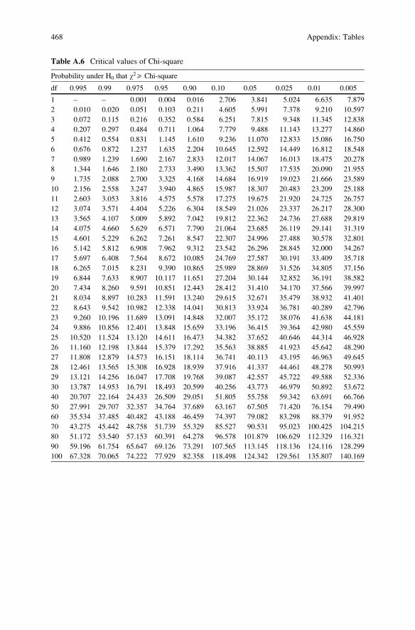
Table A.6 Critical values of Chi-square
Probability under H0 that w2r Chi-square
df 0.995 0.99 0.975 0.95 0.90 0.10 0.05 0.025 0.01 0.005
1 – – 0.001 0.004 0.016 2.706 3.841 5.024 6.635 7.879
2 0.010 0.020 0.051 0.103 0.211 4.605 5.991 7.378 9.210 10.597
3 0.072 0.115 0.216 0.352 0.584 6.251 7.815 9.348 11.345 12.838
4 0.207 0.297 0.484 0.711 1.064 7.779 9.488 11.143 13.277 14.860
5 0.412 0.554 0.831 1.145 1.610 9.236 11.070 12.833 15.086 16.750
6 0.676 0.872 1.237 1.635 2.204 10.645 12.592 14.449 16.812 18.548
7 0.989 1.239 1.690 2.167 2.833 12.017 14.067 16.013 18.475 20.278
8 1.344 1.646 2.180 2.733 3.490 13.362 15.507 17.535 20.090 21.955
9 1.735 2.088 2.700 3.325 4.168 14.684 16.919 19.023 21.666 23.589
10 2.156 2.558 3.247 3.940 4.865 15.987 18.307 20.483 23.209 25.188
11 2.603 3.053 3.816 4.575 5.578 17.275 19.675 21.920 24.725 26.757
12 3.074 3.571 4.404 5.226 6.304 18.549 21.026 23.337 26.217 28.300
13 3.565 4.107 5.009 5.892 7.042 19.812 22.362 24.736 27.688 29.819
14 4.075 4.660 5.629 6.571 7.790 21.064 23.685 26.119 29.141 31.319
15 4.601 5.229 6.262 7.261 8.547 22.307 24.996 27.488 30.578 32.801
16 5.142 5.812 6.908 7.962 9.312 23.542 26.296 28.845 32.000 34.267
17 5.697 6.408 7.564 8.672 10.085 24.769 27.587 30.191 33.409 35.718
18 6.265 7.015 8.231 9.390 10.865 25.989 28.869 31.526 34.805 37.156
19 6.844 7.633 8.907 10.117 11.651 27.204 30.144 32.852 36.191 38.582
20 7.434 8.260 9.591 10.851 12.443 28.412 31.410 34.170 37.566 39.997
21 8.034 8.897 10.283 11.591 13.240 29.615 32.671 35.479 38.932 41.401
22 8.643 9.542 10.982 12.338 14.041 30.813 33.924 36.781 40.289 42.796
23 9.260 10.196 11.689 13.091 14.848 32.007 35.172 38.076 41.638 44.181
24 9.886 10.856 12.401 13.848 15.659 33.196 36.415 39.364 42.980 45.559
25 10.520 11.524 13.120 14.611 16.473 34.382 37.652 40.646 44.314 46.928
26 11.160 12.198 13.844 15.379 17.292 35.563 38.885 41.923 45.642 48.290
27 11.808 12.879 14.573 16.151 18.114 36.741 40.113 43.195 46.963 49.645
28 12.461 13.565 15.308 16.928 18.939 37.916 41.337 44.461 48.278 50.993
29 13.121 14.256 16.047 17.708 19.768 39.087 42.557 45.722 49.588 52.336
30 13.787 14.953 16.791 18.493 20.599 40.256 43.773 46.979 50.892 53.672
40 20.707 22.164 24.433 26.509 29.051 51.805 55.758 59.342 63.691 66.766
50 27.991 29.707 32.357 34.764 37.689 63.167 67.505 71.420 76.154 79.490
60 35.534 37.485 40.482 43.188 46.459 74.397 79.082 83.298 88.379 91.952
70 43.275 45.442 48.758 51.739 55.329 85.527 90.531 95.023 100.425 104.215
80 51.172 53.540 57.153 60.391 64.278 96.578 101.879 106.629 112.329 116.321
90 59.196 61.754 65.647 69.126 73.291 107.565 113.145 118.136 124.116 128.299
100 67.328 70.065 74.222 77.929 82.358 118.498 124.342 129.561 135.807 140.169
468 Appendix: Tables

References and Further Readings
Achtert E, Bohm C, Kroger P (2006) DeLi-Clu: boosting robustness, completeness, usability,
and efficiency of hierarchical clustering by a closest pair ranking. In: LNCS: Advances in
knowledge discovery and data mining (Lecture notes in computer science), vol 3918.
doi:10.1007/11731139_16; pp 119–128
Achtert E, Bohm C, Kriegel HP, Kroger P, Muller-Gorman I, Zimek A (2007a) Detection and
visualization of subspace cluster hierarchies. In: LNCS: Advances in databases: concepts,
systems and applications (Lecture notes in computer science), vol 4443. doi:10.1007/978-3-
540-71703-4_15; pp 152–163
Achtert E, Bohm C, Kriegel HP, Kroger P, Zimek A (2007b) On exploring complex relationships
of correlation clusters. In: 19th international conference on scientific and statistical database
management (SSDBM 2007), Banff, Canada, p 7. doi:10.1109/SSDBM.2007.21
Ader HJ (2008) Chapter 14: Phases and initial steps in data analysis. In: Ader HJ,
Mellenbergh GJ (eds) (with contributions by Hand DJ) Advising on research methods: a
consultant’s companion. Johannes van Kessel Publishing, Huizen, pp 333–356
Agresti A (1996) An introduction to categorical data analysis. Wiley, Hoboken, New York
Agresti A (2002) Categorical data analysis. Wiley-Interscience, New York
Agresti A (2007) Building and applying logistic regression models. In: An introduction to
categorical data analysis. Wiley, Hoboken, p 138
Aldrich J (2005) Fisher and regression. Stat Sci 20(4):401–417. doi:10.1214/
088342305000000331, JSTOR 20061201
Armstrong JS (2012) Illusions in regression analysis. Int J Forecast 28(3):689–694, http://upenn.
academia.edu/JArmstrong/Papers/1162346/Illusions_in_Regression_Analysis
Baba K, Shibata R, Sibuya M (2004) Partial correlation and conditional correlation as
measures of conditional independence. Aust NZ J Stat 46(4):657–664. doi:10.1111/j.1467-
842X.2004.00360.x
Babbie E (2004) The practice of social research, 10th edn. Thomson Learning Inc., Wadsworth
Bailey RA (2008) Design of comparative experiments. Cambridge University Press,
Cambridge, UK
Balakrishnan N (1991) Handbook of the logistic distribution. Marcel Dekker, Inc, New York
Bandalos DL, Boehm-Kaufman MR (2009) Four common misconceptions in exploratory factor
analysis. In: Lance CE, Vandenberg RJ (eds) Statistical and methodological myths and urban
legends: doctrine, verity and fable in the organizational and social sciences. Routledge,
New York, pp 61–87
Bartholomew DJ, Steele F, Galbraith J, Moustaki I (2008) Analysis of multivariate social science
data, 2nd edn. Chapman & Hall/Crc, New York
J.P. Verma, Data Analysis in Management with SPSS Software,DOI 10.1007/978-81-322-0786-3, # Springer India 2013
469

Blair RC (1981) A reaction to ‘Consequences of failure to meet assumptions underlying the fixed
effects analysis of variance and covariance’. Rev Educ Res 51:499–507
Borg I, Groenen P (2005) Modern multidimensional scaling: theory and applications, 2nd edn.
Springer, New York, pp 207–212
Box GEP (1953) Non-normality and tests on variances. Biometrika 40(3/4):318–335, JSTOR
2333350
Buda A, Jarynowski A (2010) Life-time of correlations and its applications, vol 1. Wydawnictwo
51 Niezalezne, Wrocław
Calinski T, Kageyama S (2000) Block designs: a randomization approach, Volume I: Analysis, vol
150, Lecture notes in statistics. Springer, New York
Cameron AC, Windmeijer FAG (1997) An R-squared measure of goodness of fit for some
common nonlinear regression models. J Econom 77(2):329–342
Cattell RB (1966) The scree test for the number of factors. Multivar Behav Res 1(2):245–276.
University of Illinois, Urbana-Champaign, IL
Chatfield C (1993) Calculating interval forecasts. J Bus Econ Stat 11:121–135
Chernoff H, Lehmann EL (1954) The use of maximum likelihood estimates in w2 tests for
goodness-of-fit. Ann Math Stat 25(3):579–586. doi:10.1214/aoms/1177728726
Chow SL (1996) Statistical significance: rationale, validity and utility, vol 1, Introducing statistical
methods. Sage Publications Ltd, London
Christensen R (2002) Plane answers to complex questions: the theory of linear models, 3rd edn.
Springer, New York
Clatworthy J, Buick D, Hankins M, Weinman J, Horne R (2005) The use and reporting of cluster
analysis in health psychology: a review. Br J Health Psychol 10:329–358
Cliff N, Keats JA (2003) Ordinal measurement in the behavioral sciences. Erlbaum, Mahwah
Cohen J (1994) The earth is round (p < .05). Am Psychol 49(12):997–1003, This paper lead to the
review of statistical practices by the APA. Cohen was a member of the Task Force that did
the review
Cohen Jacob, Cohen Patricia, West Stephen G, Aiken Leona S (2002) Applied, multiple regression
– correlation analysis for the behavioral sciences. Routledge Academic, New York
Cohen J, Cohen P, West SG, Aiken LS (2003) Applied multiple regression/correlation analysis for
the behavioral sciences, 3rd edn. Erlbaum, Mahwah
Corder GW, Foreman DI (2009) Nonparametric statistics for non-statisticians: a step-by-step
approach. Wiley, Hoboken, New Jersy
Cox TF, Cox MAA (2001) Multidimensional scaling. Chapman and Hall, Boca Raton
Cox DR, Hinkley DV (1974) Theoretical Statistics, Chapman & Hall
Cox DR, Reid N (2000) The theory of design of experiments. Chapman & Hall/CRC, Fl
Cramer D (1997) Basic statistics for social research. Routledge, London
Critical Values of the Chi-Squared Distribution. NIST/SEMATECH e-Handbook of Statistical
Methods. National Institute of Standards and Technology. http://www.itl.nist.gov/div898/
handbook/eda/section3/eda3674.htm
Crown WH (1998) Statistical models for the social and behavioral sciences: multiple regression
and limited-dependent variable models. Praeger, Westport/London
Darlington RB (2004) Factor analysis. http://comp9.psych.cornell.edu/Darlington/factor.htm.
Retrieved 22 July 2011
David W Hosmer, Stanley Lemeshow (2000) Applied Logistic Regression (2nd ed.). John Wiley
& Sons, Hoboken, NJ
Devlin SJ, Gnanadesikan R, Kettenring JR (1975) Robust estimation and outlier detection with
correlation coefficients. Biometrika 62(3):531–545. doi:10.1093/biomet/62.3.531. JSTOR
2335508
Ding C, He X (July 2004) K-means clustering via principal component analysis. In: Proceedings of
international conference on machine learning (ICML 2004), pp 225–232. http://ranger.uta.edu/
~chqding/papers/KmeansPCA1.pdf
470 References and Further Readings
Dobson AJ, Barnett AG (2008) Introduction to generalized linear models, 3rd edn. Chapman and
Hall/CRC, Boca Raton
Dodge Y (2003) The Oxford dictionary of statistical terms. Oxford University Press, Oxford
Dowdy S, Wearden S (1983) Statistics for research. Wiley, New York
Draper NR, Smith H Applied regression analysis Wiley series in probability and statistics. Wiley,
New York
Duda RO, Hart PE, Stork DH (2000) Pattern classification, 2nd edn. Wiley Interscience, New York
Fisher RA (1921) On the probable error of a coefficient of correlation deduced from a small sample
(PDF). Metron 1(4):3–32. http://hdl.handle.net/2440/15169. Retrieved 25 Mar 2011
Fisher RA (1924) The distribution of the partial correlation coefficient. Metron 3(3–4):329–332.
http://digital.library.adelaide.edu.au/dspace/handle/2440/15182
Fisher RA (1925) Statistical methods for research workers. Oliver and Boyd, Edinburgh, p 43
Fisher RA (1954) Statistical methods for research workers, 12th edn. Oliver and Boyd, Edinburgh,
London
Flyvbjerg B (2011) Case study. In: Denzin NK, Lincoln YS (eds) The Sage handbook of
qualitative research, 4th edn. Sage, Thousand Oaks, pp 301–316
Fotheringham AS, Brunsdon C, Charlton M (2002) Geographically weighted regression: the
analysis of spatially varying relationships. Wiley, Hoboken, NJ
Fowlkes EB, Mallows CL (1983) A method for comparing two hierarchical clusterings. J Am Stat
Assoc 78:553–569
Fox J (1997) Applied regression analysis, linear models and related methods. Sage, Thousand
Oaks, California
Francis DP, Coats AJ, Gibson D (1999) How high can a correlation coefficient be? Int J Cardiol
69:185–199. doi:10.1016/S0167-5273(99)00028-5
Freedman DA (2005) Statistical models: theory and practice. Cambridge University Press,
Cambridge
Freedman DA et al (2007) Statistics, 4th edn. W.W. Norton & Company, New York
Friedman JH (1989) Regularized discriminant analysis. J Am Stat Assoc (American Statistical
Association) 84(405):165–175. doi:10.2307/2289860. JSTOR 2289860. MR0999675.
http://www.slac.stanford.edu/cgi-wrap/getdoc/slac-pub-4389.pdf
Gayen AK (1951) The frequency distribution of the product moment correlation coefficient in
random samples of any size draw from non-normal universes. Biometrika 38:219–247.
doi:10.1093/biomet/38.1-2.219
Gibbs Jack P, Poston JR, Dudley L (1975) The division of labor: conceptualization and related
measures. Soc Forces 53(3):468–476
Glover DM, Jenkins WJ, Doney SC (2008) Least squares and regression techniques, goodness of
fit and tests, non-linear least squares techniques. Woods Hole Oceanographic Institute, Woods
Hole
Gorsuch RL (1983) Factor analysis. Lawrence Erlbaum, Hillsdale
Green P (1975) Marketing applications of MDS: assessment and outlook. J Market 39(1):24–31.
doi:10.2307/1250799
Greenwood PE, Nikulin MS (1996) A guide to chi-squared testing. Wiley, New York
Hardin J, Hilbe J (2003) Generalized estimating equations. Chapman and Hall/CRC, London
Hardin J, Hilbe J (2007) Generalized linear models and extensions, 2nd edn. Stata Press, College
Station
Harlow L, Mulaik SA, Steiger JH (eds) (1997) What if there were no significance tests? Lawrence
Erlbaum Associates, Mahwah, NJ
Hastie TJ, Tibshirani RJ (1990) Generalized additive models. Chapman & Hall/CRC, New York
Hempel CG (1952) Fundamentals of concept formation in empirical science. The University of
Chicago Press, Chicago, p 33
Hettmansperger TP, McKean JW (1998) Robust nonparametric statistical methods, 1st edn,
Kendall’s library of statistics 5. Edward Arnold, London, p xiv+467
Hilbe JM (2009) Logistic regression models. Chapman & Hall/CRC Press, Boca Raton, FL
Hinkelmann K, Kempthorne O (2008) Design and analysis of experiments. I and II, 2nd edn.,
Wiley, New York
References and Further Readings 471

Hosmer DW, Lemeshow S (2000) Applied logistic regression, 2nd edn. Wiley, New York/
Chichester
Huang Z (1998a) Extensions to the K-means algorithm for clustering large datasets with categori-
cal values. Data Mining Knowl Discov 2:283–304
Huang Z (1998b) Extensions to the k-means algorithm for clustering large data sets with categori-
cal values. Data Mining Knowl Discov 2:283–304
Hubbard R, Armstrong JS (2006) Why we don’t really know what statistical significance means:
implications for educators. J Market Educ 28(2):114. doi:10.1177/0273475306288399
Hubbard R, Parsa AR, Luthy MR (1997) The spread of statistical significance testing in psychol-
ogy: the case of the Journal of Applied Psychology. Theory Psychol 7:545–554
Hutcheson G, Sofroniou N (1999) The multivariate social scientist: introductory statistics using
generalized linear models. Sage Publications, Thousand Oaks
Jardine N, Sibson R (1968) The construction of hierarchic and non-hierarchic classifications.
Comput J 11:177
Jones LV, Tukey JW (December 2000) A sensible formulation of the significance test. Psychol
Methods 5(4):411–414. doi:10.1037/1082-989X.5.4.411. PMID 11194204. http://content.apa.
org/journals/met/5/4/411
Kempthorne O (1952) The design and analysis of experiments, Wiley, New York
Kendall MG (1955) Rank correlation methods. Charles Griffin & Co., London
Kendall MG, Stuart A (1973) The advanced theory of statistics, vol 2: Inference and relationship.
Griffin, London
Kenney JF, Keeping ES (1951) Mathematics of statistics, Pt. 2, 2nd edn. Van Nostrand, Princeton
Kirk RE (1995) Experimental design: procedures for the behavioral sciences, 3rd edn. Brooks/
Cole, Pacific Grove
Kriegel HP, Kroger P, Schubert E, Zimek A (2008) A general framework for increasing
the robustness of PCA-based correlation clustering algorithms. In: Scientific and statistical
database management. (Lecture notes in computer science 5069). doi:10.1007/978-3-540-
69497-7_27; ISBN 978-3-540-69476-2, p 418
Kruskal JB, Wish M (1978) Multidimensional scaling, Sage University paper series on quantita-
tive application in the social sciences. Sage Publications, Beverly Hills/London, pp 7–11
Kutner H, Nachtsheim CJ, Neter J (2004) Applied linear regression models, 4th edn. McGraw-
Hill/Irwin, Boston, p 25
Larsen RJ, Stroup DF (1976) Statistics in the real world. Macmillan, New York
Ledesma RD, Valero-Mora P (2007) Determining the number of factors to retain in EFA: an easy-
to-use computer program for carrying out parallel analysis. Pract Assess Res Eval 12(2):1–11
Lee Y, Nelder J, Pawitan Y (2006) Generalized linear models with random effects: unified analysis
via H-likelihood, Chapman & Hall/CRC, Boca Raton, FL
Lehmann EL (1970) Testing statistical hypothesis, 5th edn. Wiley, New York
Lehmann EL (1992) Introduction to Neyman and Pearson (1933) on the problem of the most
efficient tests of statistical hypotheses. In: Kotz S, Johnson NL (eds) Breakthroughs in
statistics, vol 1. Springer, New York (Followed by reprinting of the paper)
Lehmann EL (1997) Testing statistical hypotheses: the story of a book. Stat Sci 12(1):48–52
Lehmann EL, Romano JP (2005) Testing statistical hypotheses, 3Eth edn. Springer, New York
Lentner M, Bishop T (1993) Experimental design and analysis, 2nd edn. Valley Book Company,
Blacksburg
Lewis-Beck MS (1995) Data analysis: an introduction. Sage Publications Inc, Thousand Oaks.
California
Lindley DV (1987) “Regression and correlation analysis,” New Palgrave: A dictionary of
economics, vol 4, pp 120–123.
Lomax RG (2007) Statistical concepts: a second course, Lawrence Erlbaum Associates, NJ
MacCallum R (1983) A comparison of factor analysis programs in SPSS, BMDP, and SAS.
Psychometrika 48(48):doi:10.1007/BF02294017
Mackintosh NJ (1998) IQ and human intelligence. Oxford University Press, Oxford, pp 30–31
Maranell GM (2007) Chapter 31. In: Scaling: a sourcebook for behavioral scientists. Aldine
Transaction, New Brunswick/London, pp 402–405
472 References and Further Readings

Mark J, Goldberg MA (2001) Multiple regression analysis and mass assessment: a review of the
issues. Apprais J Jan:89–109
Mayo DG, Spanos A (2006) Severe testing as a basic concept in a Neyman-Pearson philosophy of
induction. Br J Philos Sci 57(2):323. doi:10.1093/bjps/axl003
McCloskey DN, Ziliak ST (2008) The cult of statistical significance: how the standard error costs
us jobs, justice, and lives. University of Michigan Press, Ann Arbor., MI
McCullagh P, Nelder J (1989) Generalized linear models, 2nd edn. Chapman and Hall/CRC, Boca
Raton
Mellenbergh GJ (2008) Chapter 8: Research designs: testing of research hypotheses. In: Ader HJ,
Mellenbergh GJ (eds) (with contributions by D.J. Hand) Advising on research methods:
a consultant’s companion. Johannes van Kessel Publishing, Huizen, pp 183–209
Menard S (2002) Applied logistic regression analysis, Quantitative applications in the social
sciences, 2nd edn. Sage Publications, Thousand Oaks, California
Mezzich JE, Solomon H (1980) Taxonomy and behavioral science. Academic Press, Inc., New
York
Michell J (1986) Measurement scales and statistics: a clash of paradigms. Psychol Bull 3:398–407
Miranda A, Le Borgne YA, Bontempi G (2008) New routes from minimal approximation error to
principal components. Neural Process Lett 27(3):197–207, Springer
Milligan GW (1980) An examination of the effect of six types of error perturbation on fifteen
clustering algorithms. Psychometrika 45:325–342
Morrison D, Henkel R (eds) (2006/1970) The significance test controversy. AldineTransaction,
New Brunswick
Nagelkerke (1991) A note on a general definition of the coefficient of determination. Biometrika
78(3):691–692
Narens L (1981) On the scales of measurement. J Math Psychol 24:249–275
Nelder J, Wedderburn R (1972) Generalized linear models. J R Stat Soc A (General). 135
(3):370–384 (Blackwell Publishing). doi:10.2307/2344614. JSTOR 2344614
Nemes S, Jonasson JM, Genell A, Steineck G (2009) Bias in odds ratios by logistic regression
modelling and sample size. BMC Med Res Methodol 9:56, BioMedCentral
Neyman J, Pearson ES (1933) On the problem of the most efficient tests of statistical hypotheses.
Phil Trans R Soc A 231:289–337. doi:10.1098/rsta.1933.0009
Nickerson RS (2000) Null hypothesis significance tests: a review of an old and continuing
controversy. Psychol Methods 5(2):241–301
Pearson K, Fisher RA, Inman HF (1994) Karl Pearson and R. A. Fisher on statistical tests: a 1935
exchange from nature. Am Stat 48(1):2–11
Perriere G, Thioulouse J (2003) Use of correspondence discriminant analysis to predict the
subcellular location of bacterial proteins. Comput Methods Progr Biomed 70:99–105
Plackett RL (1983) Karl Pearson and the Chi-squared test. Int Stat Rev (International Statistical
Institute (ISI)) 51(1):59–72. doi:10.2307/1402731
Rahman NA (1968) A course in theoretical statistics. Charles Griffin and Company, London
Rand WM (1971) Objective criteria for the evaluation of clustering methods. J Am Stat Assoc
(American Statistical Association) 66(336):846–850. doi:10.2307/2284239, JSTOR 2284239
Rawlings JO, Pantula SG, Dickey DA (1998) Applied regression analysis: a research tool, 2nd edn.
Springer, New York
Rodgers JL, Nicewander WA (1988) Thirteen ways to look at the correlation coefficient. Am Stat
42(1):59–66
Rozeboom WW (1966) Scaling theory and the nature of measurement. Synthese 16:170–233
Rummel RJ (1976) Understanding correlation. http://www.hawaii.edu/powerkills/UC.HTM
Schervish MJ (1987) A review of multivariate analysis. Stat Sci 2(4):396–413. doi:10.1214/ss/
1177013111, ISSN 0883-4237. JSTOR 2245530
Schervish M (1996) Theory of statistics. Springer, New York, p 218. ISBN 0387945466
Sen PK, Anderson TW, Arnold SF, Eaton ML, Giri NC, Gnanadesikan R, Kendall MG, Kshirsagar
AM et al (1986) Review: contemporary textbooks on multivariate statistical analysis:
References and Further Readings 473
a panoramic appraisal and critique. J Am Stat Assoc 81(394):560–564. doi:10.2307/2289251,
ISSN 0162–1459. JSTOR 2289251.(Pages 560–561)
Sheppard AG (1996) The sequence of factor analysis and cluster analysis: differences in segmen-
tation and dimensionality through the use of raw and factor scores. Tour Anal 1(Inaugural
Volume):49–57
Sheskin DJ (2007) Handbook of parametric and nonparametric statistical procedures, 4th edn.
Chapman & Hall/CRC, Boca Raton
Stanley L (1969) Measuring population diversity. Am Soc Rev 34(6):850–862
StatSoft, Inc (2010) Semi-partial (or part) correlation. In: Electronic statistics textbook. StatSoft,
Tulsa, Accessed 15 Jan 2011
Steel RGD, Torrie JH (1960) Principles and procedures of statistics. McGraw-Hill, New York,
pp 187–287
Stigler SM (1989) Francis Galton’s account of the invention of correlation. Stat Sci 4(2):73–79.
doi:10.1214/ss/1177012580. JSTOR 2245329
Swanson DA (1976) A sampling distribution and significance test for differences in qualitative
variation. Soc Forces 55(1):182–184
Szekely GJ, Rizzo ML (2009) Brownian distance covariance. Ann Appl Stat 3/4:1233–1303.
doi:10.1214/09-AOAS312, Reprint
Tabachnick B, Fidell L (1996) Using multivariate statistics, 3rd edn. Harper Collins, New York
Tabachnick BG, Fidell LS (2007) Chapter 4: Cleaning up your act. Screening data prior to
analysis. In: Tabachnick BG, Fidell LS (eds) Using multivariate statistics, 5th edn. Pearson
Education, Inc./Allyn and Bacon, Boston, pp 60–116
Taylor JR (1997) An introduction to error analysis. University Science Books, Sausalito, CA
Thomas G (2011) How to do your case study. Sage, Thousand Oaks, London
Torgerson WS (1958) Theory & methods of scaling. Wiley, New York. ISBN 0898747228
Trochim WMK (2006) Descriptive statistics. Research Methods Knowledge Base. http://www.
socialresearchmethods.net/kb/statdesc.php. Retrieved 14 Mar 2011
Velleman PF, Wilkinson L (1993) Nominal, ordinal, interval, and ratio typologies are misleading.
Am Stat (American Statistical Association) 47(1):65–72. doi:10.2307/2684788, JSTOR
2684788
Venables WN, Ripley BD (2002) Modern applied statistics with S, 4th edn. Springer, New York
von Eye A (2005) Review of Cliff and Keats, ordinal measurement in the behavioral sciences.
Appl Psychol Meas 29:401–403
Wilcox Allen R (1973) Indices of qualitative variation and political measurement. West Polit Q 26
(2):325–343
Wilcox RR (2005) Introduction to robust estimation and hypothesis testing. Elsevier Academic
Press, San Diego, CA
Wilkinson L (1999) Statistical methods in psychology journals; guidelines and explanations. Am
Psychol 54(8):594–604
Wood S (2006) Generalized additive models: an introduction with R. Chapman & Hall/CRC, Boca
Raton, FL
Yin RK (2009) Case study research: design and methods, 4th edn. SAGE Publications, Thousand
Oaks
Yu H, Yang J (2001) A direct LDA algorithm for high-dimensional data – with application to face
recognition. Pattern Recognit 34(10):2067–2069
Yule GU, Kendall MG (1950) An introduction to the theory of statistics, 14th edn. Charles Griffin
& Co, London
Zeger SL, Liang K-Y, Albert PS (1988) Models for longitudinal data: a generalized estimating
equation approach. Biometrics (International Biometric Society) 44(4):1049–1060.
doi:10.2307/2531734. JSTOR 2531734, PMID 3233245
Zhang XHD (2011) Optimal high-throughput screening: practical experimental design and data
analysis for genome-scale RNAi research. Cambridge University Press, Cambridge
474 References and Further Readings

Index
A
Absolute variability, 49
Acceptance region, 171
Adjusted R2, 146, 148
Agglomeration schedule, 329, 340, 348–349
to know how should cluster be
combined, 344
Agglomerative clustering, 322–324,
326, 328
linkage methods, 324
centroid method, 324
variance methods, 324
Akaike information criterion, 328
Alternative hypothesis, 170–171, 173–177,
179–183, 222, 225, 229, 262
Analysis of covariance
assumptions, 298
computation with SPSS, 298
efficiency of ANCOVA over ANOVA, 298
graphical explanation, 293
introductory concepts, 292
model, 294
what we do, 296
when to use, 297
Analysis of variance
to know difference between clusters, 353
Factorial, 223, 257
multivariate, 224, 258
one way, 171, 221–222, 228,
255–256, 260, 291–292
repeated measure, 223, 258
two way, 255–266
Analytical studies, 2, 25
ANOVA table, 226, 264
Applied studies, 3
Assignment matrix, 392
Atomic clusters, 323
Attribute based approach of multidimensional
scaling, 446, 447
Attribute mutually exclusive, 6
B
Bartlett’s test of sphericity, 365, 375
Binary logistic regression, 413
Binary variable, 415
Box’s M test, 393, 396
C
Canonical correlation, 394, 404
Canonical root, 392
Categorical variable, 5, 72
Central limit theorem, 222
Characteristics root, 363
Chebyshev distance, 320
Chi square test, 3, 72, 417–418
additive properties, 71
application, 73
assumptions, 73
crosstab, 69–70, 88, 92
advantages, 70
statistics used, 70
for goodness of fit, 73
precautions in using, 78
situations for using, 80
statistic, 69–70
steps in computing, 72
testing equal occurrence hypothesis with
SPSS, 81
for testing independence of attributes, 76
testing significance of association with
SPSS, 87
testing the significance in SPSS, 78
J.P. Verma, Data Analysis in Management with SPSS Software,DOI 10.1007/978-81-322-0786-3, # Springer India 2013
475

Classification matrix, 392, 395, 404, 405
Cluster analysis, 318
assumptions, 331
procedure, 330
situation suitable for cluster analysis, 331
solution with SPSS, 333
steps in cluster analysis, 332
terminologies used, 318
Clustering criteria, 322
Clustering procedure, 321
hierarchical clustering, 322
nonhierarchical clustering(k-means), 326
two-step clustering, 327
Cluster membership, 354
Coefficient of determination R2, 134, 137
Coefficient of variability, 44
Coefficient of variation, 30, 48
Communality, 360, 362–363, 375
Concomitant variable, 292
Confidence interval, 48
Confirmatory study, 149, 360–361, 392, 399–400
Confusion matrix, 392
Contingency coefficient, 79
Contingency table, 69–70, 73, 76, 79, 178, 262
Correlation coefficient, 3, 104, 141, 176
computation, 106
ecological fallacy, 110
limitations, 111
misleading situations, 110
properties, 108
testing the significance, 111
unexplained causative relationship, 110
Correlation matrix, 105
computation, 106
computing with SPSS, 117
situations for application, 115
Cox and Snell’s R2, 435
Cramer’s V, 80
Critical difference, 227, 265
Critical region, 171, 175, 183, 185
Critical value, 50, 52, 111, 170–175, 182–185
Crosstab, 69–70, 88, 92
D
Data Analysis, 2, 3
Data cleaning, 9
Data mining, 1
Data warehousing, 1
Degrees of freedom, 70–72, 76, 111, 171,
177–179, 181–183, 185, 191,
226–227, 259–260, 263–265, 417
Dendogram, 322–323, 329–330, 332, 346
plotting cluster distances, 349
Dependent variable, 6
Descriptive research, 30
Descriptive statistics, 10, 29–31, 365
computation with SPSS, 54
Descriptive study, 2, 29, 53
Design of experiments, 222
Detection of errors
using frequencies, 10
using logic checks, 10
using mean and standard deviation, 10
using minimum and maximum scores, 10
Deviance, 416, 418–419, 434
Deviance statistic, 416, 434–435
Dimensions, 446–447
Discriminant analysis, 389
assumptions, 396
discriminant function, 390–396, 398, 404
procedure of analysis, 394
research situations for discriminant
analysis, 396
stepwise method, 392
what is discriminant analysis?, 390
Discriminant model, 390, 395
Discriminant score, 406
Dissection, 318
Dissimilarity based approach of
multidimensional scaling, 446
procedure for multidimensional scaling,
446
steps for solution, 446
Dissimilarity matrix, 445
Dissimilarity measures, 344, 446
Distance matrix, 322, 446, 447
Distance measure, 318
Distances, 445
Distribution free tests, 3
E
Eigenvalue, 361, 363, 365, 393
Equal occurrence hypothesis, 69
Error variance, 256–257, 259, 262, 292,
298, 419
Euclidean distance, 319–320, 324,
329, 331
Euclidean space, 320
Experimental error, 292
Exploratory study, 149, 360, 392, 430
Exponential function, 415
Extraneous variable, 6
476 Index

F
Factor, 259
Factor analysis, 359
assumptions, 366
characteristics, 367
Limitations, 367
Situations suitable for factor
analysis, 367
solutions with SPSS, 368
used in confirmatory studies, 360
used in exploratory studies, 360
what we do in factor analysis, 365
Factorial ANOVA, 223, 257
Factorial design, 223, 257–258
Factor loading, 362, 365, 366, 379
Factor matrix, 364
Final cluster centers, 350
Forward:LR method, 425, 428, 430–431,
433–434
Frequency distribution, 69
F statistic, 171, 221, 223, 226–227, 229,
262, 264–265
F test, 3, 72, 146, 182
Functions at group centroids, 396
Fusion coefficients, 333, 335, 340, 344
G
Gamma, 80
Goodness of fit, 69, 73, 417
H
Hierarchical clustering, 322, 324,
326–328, 331
agglomerative clustering, 322–323
divisive clustering, 322, 325
Homoscedasticity, 366
Homoscedastic relationships, 396
Hypothesis
alternative hypothesis, 170–171, 173–177,
179–183, 222, 225, 229, 262
non parametric, 168–169
null, 72, 74, 77, 111, 112, 169–179,
181–184, 191–193, 221–222,
225, 227, 229–230, 232, 262,
265, 280, 295, 297, 393
parametric, 168
research hypothesis, 169–170, 175,
184, 191
Hypothesis construction, 168
Hypothesis testing, 171
I
Icicle plots, 328–329, 331, 333, 335, 348
Identity matrix, 365, 375
Importing data in SPSS
from an ASCII file, 18
from the Excel file, 22
Independent variable, 6
Index of quartile variation, 46
Inductive studies, 2
Inferential studies, 2
Initial cluster centers, 349
Interaction, 224, 256, 260, 262
Inter-quartile range
lower quartile, 41, 42
upper quartile, 41, 42
Interval data, 1, 3, 4
Interval scale, 3
K
Kaiser’s criteria, 363, 365
k-means clustering, 326, 327, 332
KMO test, 365, 375
Kruskal-Wallis test
Kurtosis, 30, 49–52
L
Lambda coefficient, 79
Least significant difference (LSD) test,
227, 265
Least square method, 143
Left tailed test, 175, 184–185
Leptokurtic curve, 51–52
Level of significance, 72, 77,
111–112, 171–177, 179,
182–185, 192, 227–229,
262, 265
Likelihood ratio test, 417
Linear regression, 133, 143, 145, 292,
298, 419
Linkage methods, 324
average linkage method, 325
complete linkage method, 325
single linkage method, 325
Logistic curve, 415, 417
Logistic distribution, 419
Logistic function, 417, 421
interpretation, 422
Logistic model with mathematical equation,
421
Logistic regression, 396, 413
Index 477
Logistic regression (cont.)assumptions, 423
binary, 413
describing logistic regression, 414
equation, 417
graphical explanation, 419
important features, 423
judging efficiency, 418
multinomial, 413
research situations for logistic regression,
424
solution with SPSS, 426
steps in logistic regression, 425
understanding logistic regression, 419
Logit, 417–418, 421–422, 436
Log odds, 416, 418, 421, 436
Log transformation, 416
M
Main effect, 260
Manhattan distance, 320, 321
Mann-Whitney test, 3
Maximum likelihood, 416
Mean, 10
computation with deviation method, 34
computation with grouped data, 32
computation with ungrouped data, 31
properties, 35
Measures of central tendency
mean, 31
median, 31
mode, 31
Measures of variability
interquartile range, 41
range, 41
standard deviation, 42
Median
computation with grouped data, 37
computation with ungrouped data, 36
Median test, 3
Metric data
interval, 4
ratio, 4
Mode
bimodal, 38
computation with grouped data, 39
computation with ungrouped data, 38
drawbacks of mode, 39
unimodal, 38
Moment, 49
Monotonic transformation, 416
Multicollinearity, 115, 146–147, 366
Multidimensional scaling, 443
assumptions, 448
attribute based approach, 446
dissimilarity based approach, 446
limitations, 449
solution for multidimensional scaling, 449
what is multidimensional scaling?, 444
what we do in multidimensional scaling?,
446
Multidimensional space, 443–445
Multinomial distribution, 327
Multiple correlation, 105, 135
computation, 136
computing with SPSS, 149
properties, 135
Multiple regression, 145, 391
computation with SPSS, 148–149
limitations, 147
procedure, 146
Multivariate ANOVA
one way, 224
two way, 259
N
Nagelkerke’s R2
Natural log, 415
Negatively skewed curve, 51
Nominal data, 3
Nonhierarchical clustering(K-means), 322,
326–327, 331
Nonlinear regression, 415
Non metric data
nominal, 5
ordinal, 5
Non metric tests, 3
Nonparametric, 69
hypothesis, 169
Normal distribution, 50–52, 170, 192, 327, 424
Null hypothesis, 72, 74, 77, 111, 112,
169–179, 181–184, 191–193,
221–222, 225, 227, 229–230,
232, 262, 265, 280, 295,
297, 393
Null model, 427
O
Objects, 444
Odds, 416
Odds ratio, 416, 426, 436, 437
One sample t test, 179
One tailed test, 174–177, 184–185, 192, 194
478 Index

One way analysis of variance, 221–222, 228,
260, 291–292
computation (unequal sample size) with
SPSS, 241
assumptions, 228
computation (equal sample size) with
SPSS, 232
model, 224
Optimizing partitioning method, 327
Ordinal data, 3
Ordinary least square, 143, 391, 416–417,
419, 420
Outcome variable, 415
P
Paired t test, 191
application, 193
assumptions, 192
testing protocol, 192
Parallel threshold method, 327
Parameter, 178
Parametric test, 3
Partial correlation, 105–106, 111–112,
115–116
computation, 113
computing with SPSS, 117
limitations, 113
limits, 113
situations for application, 115
testing the significance, 113
Path analysis, 110
Pearson
chi square, 72
correlation r, 120, 321, 362
Pearson correlation distance, 321
Percentile, 52
Percentile rank, 53
Perceptual map, 331, 360, 444–445,
447–448
Perceptual mapping, 444, 445
Phi coefficient, 79
Platykurtic curve, 51–52
Point biserial correlation, 394
Pooled standard deviation, 178
Population mean
mean, 168
standard deviation, 171, 178
variance, 169, 171, 181
Population standard deviation, 48
Positively skewed curve, 51
Power of test, 173
Prediction matrix, 392
Predictive model, 414
Predictor variable, 391, 392
Primary data
from interviews, 8
by observation, 7
through logs, 8
through surveys, 8
Principal component analysis, 362, 364–365
Principle of randomization, 257, 292
Principle of replication, 257
Principles of ANOVA experiment, 222, 256
Probability density function, 71
Product moment correlation, 2, 104, 106,
113, 116, 135
Profile chart, 62–63
Proximity matrix, 321, 322, 329
to know how alike the cases are, 344
Pseudo R2, 435
p value, 78, 79, 96, 112, 113, 148, 172, 176,
177, 179, 227, 265, 273
Q
Quantitative data, 3
Questionnaire, 8
R
R2, 146, 148–149, 435
Ratio data, 3, 4, 42, 46, 145, 328
Regression analysis, 133, 149, 292
application, 149
assumptions, 145
confirmatory, 149
exploratory, 148–149
least square method, 143, 391
model, 146, 149
multiple regression, 133–134, 145–148
simple regression, 133, 138, 145, 147
Regression analysis methods
Enter, 149
stepwise, 148
Regression coefficients, 109, 138–139,
141–143, 146–148, 416, 418,
421–422, 426, 428, 433, 436
computation by deviation method, 140
computation by least square method, 144
properties, 141
significance, 146
standardized, 139, 147–148
unstandardized, 139, 146–148
Index 479

Regression equation, 133, 138, 148
least square, 144
stepwise, 136
Rejection region, 171, 174
Relative variability, 49
Repeated measure ANOVA, 223, 258
Right tailed test, 175, 184
S
Sampling distribution, 171
Sampling Technique, 2
Scheffe’s test, 227
Schwarz’s Bayesian criterion, 328
Scree plot, 363
Secondary data, 7, 9
Sequential threshold method, 327
Sigmoid curve, 417
Sign test, 3
Similarity matrix, 445
Similarity measures, 344
Single pass hierarchical methods, 332
Skewness, 49–51
SPSS
defining variables, 13
entering data, 16
preparing data file, 13
how to start, 11
Squared Euclidean distance, 319
Standard deviation
computation with ungrouped data,
42, 43
effect of change of origin and scale, 44
pooled, 178
Standard error
of kurtosis, 52
of mean, 47, 48
of skewness, 50
of standard deviation, 48
Standardized canonical discriminant function
coefficients, 395, 405
Standardized regression coefficient, 139,
147–148
Statistic, 172, 178
Statistical hypothesis, 169
Statistical inference, 167
Stress, 445, 447, 450, 452–453, 455
Subjects, 444
Sum of squares, 260, 264
between groups, 225–226
error, 263, 264
interaction, 263, 264
mean, 221, 226, 263–264
total, 143, 225–226, 231, 262–263
within groups, 221, 225–226, 260
Suppression variable, 135
Surveys, 8
Symmetric distribution, 31
Symmetrical regression equation, 139
T
t distribution, 171, 178
Test battery, 366, 379
Testing of hypothesis, 167–170, 173, 178,
183, 266
Test statistic, 52, 170, 171, 174–175,
177–178, 183–184, 192, 227
Theory of estimation, 167
Treatment, 260, 294
t statistic, 179, 182, 193
t test, 3, 72, 146, 171, 174, 181, 184, 223,
228–229, 258
computation in one sample t test with SPSS,
196
computation in paired t test with
SPSS, 209
computation in two sample t test with
SPSS, 201
for one sample, 179
for paired groups, 191
for two unrelated samples, 181
Two cluster solution, 346
Two sample t test
application, 182
assumptions, 181
Two-step cluster, 327
Two tailed test, 50, 174–176, 183, 188, 192
Two way ANOVA
advantage, 259
assumptions, 265
computation with SPSS, 272
hypothesis testing, 261
model, 261
situation for using two-way
ANOVA, 266
terminologies, 259
Type I error, 172–174, 228
Type II error, 73, 172–174
Types of data
metric, 3
nonmetric, 3
U
Unrotated factor solution, 364
Unstandardized canonical discriminant
function coefficients, 395, 404
Unstandardized regression coefficient, 138,
146–148
480 Index

V
Variable
categorical, 5
continuous, 5
dependent, 6
discrete, 5
extraneous, 6
independent, 6
Variance, 46, 178
Variance maximizing rotation, 362
Varimax rotation, 364, 366, 379
W
Wald statistics, 436
Ward’s method, 324
Wilk’s Lambda, 394, 395, 404
Within group variation, 260
Z
Z distribution, 168
Z test, 3, 168, 178
Index 481