Data Analysis and Manifold Learning Lecture 3: Graphs ...perception.inrialpes.fr/~Horaud/Courses/pdf/Horaud-DAML3.pdf · Data Analysis and Manifold Learning Lecture 3: Graphs, Graph

Data Analysis and Manifold LearningLecture 3: Graphs, Graph Matrices, and Graph

Embeddings

Radu HoraudINRIA Grenoble Rhone-Alpes, France

[email protected]://perception.inrialpes.fr/

Radu Horaud Data Analysis and Manifold Learning; Lecture 3

http://perception.inrialpes.fr/

Outline of Lecture 3

What is spectral graph theory?

Some graph notation and definitions

The adjacency matrix

Laplacian matrices

Spectral graph embedding


Material for this lecture

F. R. K. Chung. Spectral Graph Theory. 1997. (Chapter 1)

M. Belkin and P. Niyogi. Laplacian Eigenmaps forDimensionality Reduction and Data Representation. NeuralComputation, 15, 1373–1396 (2003).

U. von Luxburg. A Tutorial on Spectral Clustering. Statisticsand Computing, 17(4), 395–416 (2007). (An excellent paper)

Software:http://open-specmatch.gforge.inria.fr/index.php.Computes, among others, Laplacian embeddings of very largegraphs.


http://open-specmatch.gforge.inria.fr/index.php

Spectral graph theory at a glance

The spectral graph theory studies the properties of graphs viathe eigenvalues and eigenvectors of their associated graphmatrices: the adjacency matrix, the graph Laplacian and theirvariants.

These matrices have been extremely well studied from analgebraic point of view.

The Laplacian allows a natural link between discreterepresentations (graphs), and continuous representations, suchas metric spaces and manifolds.

Laplacian embedding consists in representing the vertices of agraph in the space spanned by the smallest eigenvectors of theLaplacian – A geodesic distance on the graph becomes aspectral distance in the embedded (metric) space.


Spectral graph theory and manifold learning

First we construct a graph from x1, . . .xn ∈ RD

Then we compute the d smallest eigenvalue-eigenvector pairsof the graph Laplacian

Finally we represent the data in the Rd space spanned by thecorrespodning orthonormal eigenvector basis. The choice ofthe dimension d of the embedded space is not trivial.

Paradoxically, d may be larger than D in many cases!


Basic graph notations and definitions

We consider simple graphs (no multiple edges or loops),G = V, E:

V(G) = v1, . . . , vn is called the vertex set with n = |V|;E(G) = eij is called the edge set with m = |E|;An edge eij connects vertices vi and vj if they are adjacent orneighbors. One possible notation for adjacency is vi ∼ vj ;The number of neighbors of a node v is called the degree of vand is denoted by d(v), d(vi) =

∑vi∼vj

eij . If all the nodes ofa graph have the same degree, the graph is regular ; Thenodes of an Eulerian graph have even degree.

A graph is complete if there is an edge between every pair ofvertices.


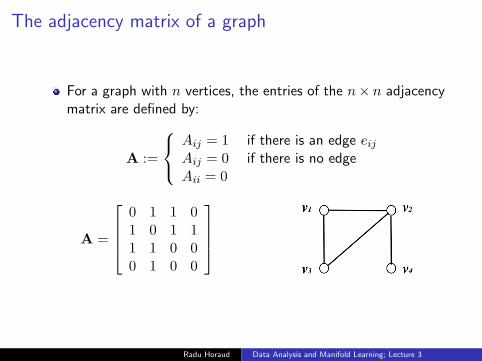
The adjacency matrix of a graph

For a graph with n vertices, the entries of the n× n adjacencymatrix are defined by:

A :=

Aij = 1 if there is an edge eijAij = 0 if there is no edgeAii = 0

A =

0 1 1 01 0 1 11 1 0 00 1 0 0


Eigenvalues and eigenvectors

A is a real-symmetric matrix: it has n real eigenvalues and itsn real eigenvectors form an orthonormal basis.

Let λ1, . . . , λi, . . . , λr be the set of distinct eigenvalues.

The eigenspace Si contains the eigenvectors associated withλi:

Si = x ∈ Rn|Ax = λix

For real-symmetric matrices, the algebraic multiplicity is equalto the geometric multiplicity, for all the eigenvalues.

The dimension of Si (geometric multiplicity) is equal to themultiplicity of λi.

If λi 6= λj then Si and Sj are mutually orthogonal.


Real-valued functions on graphs

We consider real-valued functions on the set of the graph’svertices, f : V −→ R. Such a function assigns a real numberto each graph node.

f is a vector indexed by the graph’s vertices, hence f ∈ Rn.

Notation: f = (f(v1), . . . , f(vn)) = (f1, . . . , fn) .

The eigenvectors of the adjacency matrix, Ax = λx, can beviewed as eigenfunctions.


Matrix A as an operator and quadratic form

The adjacency matrix can be viewed as an operator

g = Af ; g(i) =∑i∼j

f(j)

It can also be viewed as a quadratic form:

f>Af =∑eij

f(i)f(j)


The incidence matrix of a graph

Let each edge in the graph have an arbitrary but fixedorientation;

The incidence matrix of a graph is a |E| × |V| (m× n) matrixdefined as follows:

5 :=

5ev = −1 if v is the initial vertex of edge e5ev = 1 if v is the terminal vertex of edge e5ev = 0 if v is not in e

5 =

−1 1 0 01 0 −1 00 −1 1 00 −1 0 +1


The incidence matrix: A discrete differential operator

The mapping f −→ 5f is known as the co-boundarymapping of the graph.

(5f)(eij) = f(vj)− f(vi)−1 1 0 01 0 −1 00 −1 1 00 −1 0 +1

f(1)f(2)f(3)f(4)

=

f(2)− f(1)f(1)− f(3)f(3)− f(2)f(4)− f(2)


The Laplacian matrix of a graph

L = 5>5(Lf)(vi) =

∑vj∼vi

(f(vi)− f(vj))Connection between the Laplacian and the adjacency matrices:

L = D−A

The degree matrix: D := Dii = d(vi).

L =

2 −1 −1 0−1 3 −1 −1−1 −1 2 00 −1 0 1


Example: A graph with 10 nodes

1 2

35

9

4

67

810


The adjacency matrix

A =

0 1 1 1 0 0 0 0 0 01 0 0 0 1 0 0 0 0 01 0 0 0 0 1 1 0 0 01 0 0 0 1 0 0 1 0 00 1 0 1 0 0 0 0 1 00 0 1 0 0 0 1 1 0 10 0 1 0 0 1 0 0 0 00 0 0 1 0 1 0 0 1 10 0 0 0 1 0 0 1 0 00 0 0 0 0 1 0 1 0 0


The Laplacian matrix

L =

3 −1 −1 −1 0 0 0 0 0 0−1 2 0 0 −1 0 0 0 0 0−1 0 3 0 0 −1 −1 0 0 0−1 0 0 3 −1 0 0 −1 0 00 −1 0 −1 3 0 0 0 −1 00 0 −1 0 0 4 −1 −1 0 −10 0 −1 0 0 −1 2 0 0 00 0 0 −1 0 −1 0 4 −1 −10 0 0 0 −1 0 0 −1 2 00 0 0 0 0 −1 0 −1 0 2


The Eigenvalues of this Laplacian

Λ = [ 0.0000 0.7006 1.1306 1.8151 2.40113.0000 3.8327 4.1722 5.2014 5.7462 ]


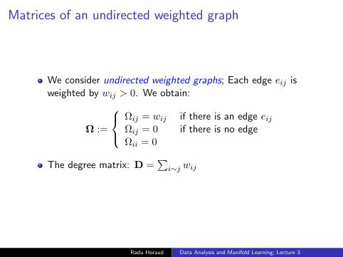
Matrices of an undirected weighted graph

We consider undirected weighted graphs; Each edge eij isweighted by wij > 0. We obtain:

Ω :=

Ωij = wij if there is an edge eijΩij = 0 if there is no edgeΩii = 0

The degree matrix: D =∑

i∼j wij


The Laplacian on an undirected weighted graph

L = D−Ω

The Laplacian as an operator:

(Lf)(vi) =∑vj∼vi

wij(f(vi)− f(vj))

As a quadratic form:

f>Lf =12

∑eij

wij(f(vi)− f(vj))2

L is symmetric and positive semi-definite ↔ wij ≥ 0.

L has n non-negative, real-valued eigenvalues:0 = λ1 ≤ λ2 ≤ . . . ≤ λn.


Other adjacency matrices

The normalized weighted adjacency matrix

ΩN = D−1/2ΩD−1/2

The transition matrix of the Markov process associated withthe graph:

ΩR = D−1Ω = D−1/2ΩND1/2


Several Laplacian matrices

The unnormalized Laplacian which is also referred to as thecombinatorial Laplacian LC ,

the normalized Laplacian LN , and

the random-walk Laplacian LR also referred to as the discreteLaplace operator.

We have:

LC = D−Ω

LN = D−1/2LCD−1/2 = I−ΩN

LR = D−1LC = I−ΩR


Relationships between all these matrices

LC = D1/2LND1/2 = DLRLN = D−1/2LCD−1/2 = D1/2LRD−1/2

LR = D−1/2LND1/2 = D−1LC


Some spectral properties of the Laplacians

Laplacian Null space Eigenvalues Eigenvectors

LC =UΛU>

u1 = 1 0 = λ1 < λ2 ≤. . . ≤ λn ≤2 maxi(di)

u>i>11 = 0,u>i uj = δij

LN =WΓW>

w1 = D1/21 0 = γ1 < γ2 ≤. . . ≤ γn ≤ 2

w>i>1D1/21 =

0,w>i wj = δij

LR =TΓT−1

T =D−1/2W

t1 = 1 0 = γ1 < γ2 ≤. . . ≤ γn ≤ 2

t>i>1D1 = 0,t>i Dtj = δij


Spectral properties of adjacency matrices

From the relationship between the normalized Laplacian andadjacency matrix: LN = I−ΩN one can see that their eigenvaluessatisfy γ = 1− δ.

Adjacency matrix Eigenvalues Eigenvectors

ΩN = W∆W>,∆ = I− Γ

−1 ≤ δn ≤ . . . ≤ δ2 <δ1 = 1

w>i wj = δij

ΩR = T∆T−1 −1 ≤ δn ≤ . . . ≤ δ2 <δ1 = 1

t>i Dtj = δij


The Laplacian of a graph with one connected component

Lu = λu.

L1 = 0, λ1 = 0 is the smallest eigenvalue.

The one vector: 1 = (1 . . . 1)>.

0 = u>Lu =∑n

i,j=1wij(u(i)− u(j))2.

If any two vertices are connected by a path, thenu = (u(1), . . . , u(n)) needs to be constant at all vertices suchthat the quadratic form vanishes. Therefore, a graph with oneconnected component has the constant vector u1 = 1 as theonly eigenvector with eigenvalue 0.


A graph with k > 1 connected components

Each connected component has an associated Laplacian.Therefore, we can write matrix L as a block diagonal matrix :

L =

L1

. . .

Lk

The spectrum of L is given by the union of the spectra of Li.

Each block corresponds to a connected component, henceeach matrix Li has an eigenvalue 0 with multiplicity 1.

The spectrum of L is given by the union of the spectra of Li.

The eigenvalue λ1 = 0 has multiplicity k.


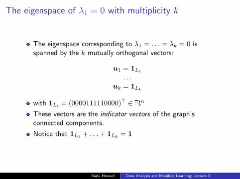
The eigenspace of λ1 = 0 with multiplicity k

The eigenspace corresponding to λ1 = . . . = λk = 0 isspanned by the k mutually orthogonal vectors:

u1 = 1L1

. . .uk = 1Lk

with 1Li = (0000111110000)> ∈ Rn

These vectors are the indicator vectors of the graph’sconnected components.

Notice that 1L1 + . . .+ 1Lk= 1


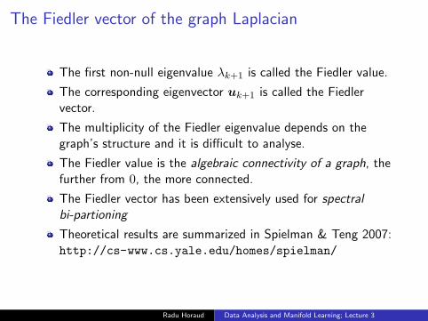
The Fiedler vector of the graph Laplacian

The first non-null eigenvalue λk+1 is called the Fiedler value.

The corresponding eigenvector uk+1 is called the Fiedlervector.

The multiplicity of the Fiedler eigenvalue depends on thegraph’s structure and it is difficult to analyse.

The Fiedler value is the algebraic connectivity of a graph, thefurther from 0, the more connected.

The Fiedler vector has been extensively used for spectralbi-partioning

Theoretical results are summarized in Spielman & Teng 2007:http://cs-www.cs.yale.edu/homes/spielman/


http://cs-www.cs.yale.edu/homes/spielman/

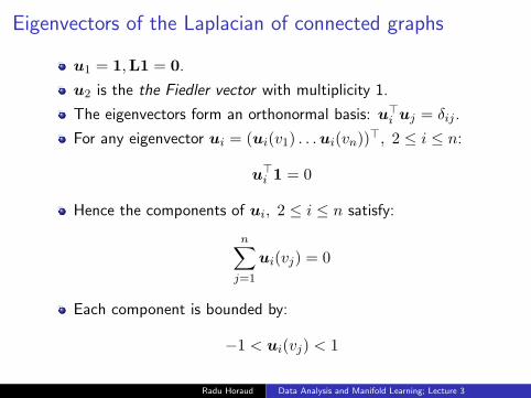
Eigenvectors of the Laplacian of connected graphs

u1 = 1,L1 = 0.

u2 is the the Fiedler vector with multiplicity 1.

The eigenvectors form an orthonormal basis: u>i uj = δij .

For any eigenvector ui = (ui(v1) . . .ui(vn))>, 2 ≤ i ≤ n:

u>i 1 = 0

Hence the components of ui, 2 ≤ i ≤ n satisfy:

n∑j=1

ui(vj) = 0

Each component is bounded by:

−1 < ui(vj) < 1


Laplacian embedding: Mapping a graph on a line

Map a weighted graph onto a line such that connected nodesstay as close as possible, i.e., minimize∑n

i,j=1wij(f(vi)− f(vj))2, or:

arg minf

f>Lf with: f>f = 1 and f>1 = 0

The solution is the eigenvector associated with the smallestnonzero eigenvalue of the eigenvalue problem: Lf = λf ,namely the Fiedler vector u2.

Practical computation of the eigenpair λ2,u2): the shiftedinverse power method (see lecture 2).


The shifted inverse power method (from Lecture 2)

Let’s consider the matrix B = A− αI as well as an eigenpairAu = λu.

(λ− α,u) becomes an eigenpair of B, indeed:

Bu = (A− αI)u = (λ− α)u

and hence B is a real symmetric matrix with eigenpairs(λ1 − α,u1), . . . (λi − α,ui), . . . (λD − α,uD)If α > 0 is choosen such that |λj − α| |λi − α| ∀i 6= j thenλj − α becomes the smallest (in magnitude) eivenvalue.

The inverse power method (in conjuction with the LUdecomposition of B) can be used to estimate the eigenpair(λj − α,uj).


Example of mapping a graph on the Fiedler vector


Laplacian embedding

Embed the graph in a k-dimensional Euclidean space. Theembedding is given by the n× k matrix F = [f1f2 . . .fk]where the i-th row of this matrix – f (i) – corresponds to theEuclidean coordinates of the i-th graph node vi.

We need to minimize (Belkin & Niyogi ’03):

arg minf 1...f k

n∑i,j=1

wij‖f (i) − f (j)‖2 with: F>F = I.

The solution is provided by the matrix of eigenvectorscorresponding to the k lowest nonzero eigenvalues of theeigenvalue problem Lf = λf .


Spectral embedding using the unnormalized Laplacian

Compute the eigendecomposition L = D−Ω.

Select the k smallest non-null eigenvalues λ2 ≤ . . . ≤ λk+1

λk+2 − λk+1 = eigengap.

We obtain the n× k matrix U = [u2 . . .uk+1]:

U =

u2(v1) . . . uk+1(v1)...

...u2(vn) . . . uk+1(vn)

u>i uj = δij (orthonormal vectors), hence U>U = Ik.

Column i (2 ≤ i ≤ k + 1) of this matrix is a mapping on theeigenvector ui.


Examples of one-dimensional mappings

u2 u3

u4 u8


Euclidean L-embedding of the graph’s vertices

(Euclidean) L-embedding of a graph:

X = Λ− 1

2k U> = [x1 . . . xj . . . xn]

The coordinates of a vertex vj are:

xj =

u2(vj)√

λ2...

uk+1(vj)√λk+1

A formal justification of using this will be provided later.


The Laplacian of a mesh

A mesh may be viewed as a graph: n = 10, 000 vertices,m = 35, 000 edges. ARPACK finds the smallest 100 eigenpairs in46 seconds.


Example: Shape embedding


Documents

Data Analysis and Manifold Learning Lecture 3: Graphs ...perception.inrialpes.fr/~Horaud/Courses/pdf/Horaud-DAML3.pdf · Data Analysis and Manifold Learning Lecture 3: Graphs, Graph