Optics Communications 297 (2013) 125–128

Contents lists available at SciVerse ScienceDirect

Optics Communications

0030-40

http://d

n Corr

E-m

journal homepage: www.elsevier.com/locate/optcom

Dark–antidark solitons in waveguide arrays with alternatingpositive–negative couplings

Aldo Auditore a,n, Matteo Conforti a, Costantino De Angelis a, Alejandro B. Aceves b

a CNISM, Dipartimento di Ingegneria dell’Informazione, Universit�a degli Studi di Brescia, Brescia 25123, Italyb Department of Mathematics, Southern Methodist University, Dallas, TX 75275, USA

a r t i c l e i n f o

Article history:

Received 22 November 2012

Received in revised form

29 January 2013

Accepted 30 January 2013Available online 21 February 2013

Keywords:

Guided waves

Binary optics

Kerr effect

Spatial solitons

18/$ - see front matter & 2013 Elsevier B.V. A

x.doi.org/10.1016/j.optcom.2013.01.068

esponding author. Tel.: þ390 340 286 0431.

ail address: aldo.auditore@ing.unibs.it (A. Aud

a b s t r a c t

We obtain dark and antidark soliton solutions in binary waveguide arrays with focusing and/or

defocusing Kerr nonlinearity and with alternating positive and negative linear couplings between

adjacent waveguides. For both stationary and moving solitons, we analyze the properties of these

solutions in the presence of uniform and nonuniform nonlinearity along the array.

& 2013 Elsevier B.V. All rights reserved.

1. Introduction

In the last years, discrete optical systems and waveguidearrays have been a very active research area in optics [1]. Binarywaveguide arrays in particular have been studied because theirintrinsic two bands structure can be very helpful in order tocontrol wave propagation in the linear and nonlinear regimes[2–4]. More recently, the interplay between plasmonic waveguid-ing and periodicity has been also considered, inasmuch asplasmonic confinement offers an extra degree of freedom to beusefully exploited in all optical devices [5–8].

In this framework solitons represent an important class ofsolutions, as their particle like behavior can be very useful forswitching applications and their peculiar features often representan invaluable tool to understand the overall dynamics of thesystem in the nonlinear regime. This certainly explains the hugeeffort that the scientific community has put in finding solitonsolutions in these systems [4,9–14].

It is well known that in nonlinear discrete systems as thosedescribing light propagation in waveguide arrays, bright localizedmodes may exist in the form of gap solitons when a gap opens in thelinear dispersion relation [13,15]. On the other hand, without theband gap in the linear dispersion relation, a forbidden frequencyregion can still exist for a nonuniform nonlinear response andsolitons sitting on a pedestal can be found [14,16,17]. Among thesituations where the nonuniform nonlinearity can be exploited it is

ll rights reserved.

itore).

certainly worth quoting the case of the linear–nonlinear interlacedwaveguide arrays [18].

In previous papers we have used a continuous approximation toexploit bright solitary wave solutions of this system [13] and wehave then used a fully discrete model to explore the existence andstability of solitons sitting on a nonzero background [14]. In thispaper we extend the continuous approximation to the case of anonzero background and we demonstrate that this continuousapproximation can capture many features of the discrete system;remarkably we also show that the continuum approximation gives areasonable description of discrete states even when they are con-fined to a very small number of sites.

2. Physical settings and theoretical analysis

According to the coupled mode theory and taking into accountthird-order nonlinearities in the form of a pure Kerr effect, thefield amplitude propagation in a binary waveguide array can bedescribed by the following equations [10,13]:

iE0nzþbnE0nþCn�1E0n�1þCnþ1E0nþ1þwn9E0n9

2E0n ¼ 0

where E0n is the amplitude of the modal field of the n-thwaveguide, bn is the propagation constant of each waveguide,wn is the site-dependent nonlinear coefficient, and Cn71 is thecoupling coefficient of the n-th waveguide with the ðn71Þ-thwaveguides. In our case Cn�1 ¼ C1 and Cnþ1 ¼ C2 when n is even,whereas Cn�1 ¼ C2 and Cnþ1 ¼ C1 when n is odd. Then, performingthe transformation E0n ¼ En expðibzÞ, we can separately considerthe mode amplitudes in the even and odd waveguides. In this waythe field amplitude propagation can be described by the following

−5 0 50

0.5

1

1.5

n

|An|

−5 0 50

0.5

1

1.5

n

|Bn|

Fig. 1. Comparison between approximated soliton states obtained from the

continuum limit (blue crosses and dashed line) and exact numerical results

obtained using the Newton conjugate-gradient method (red open circles). With

reference to Eq. (1) here we set g1 ¼ 1, g2 ¼ 0, C1 ¼�1, C2 ¼ 1, Db¼ 0 and

limn-719An9¼ffiffiffi2p

. (a) Even sites. (b) Odd sites. (For interpretation of the

references to color in this figure caption, the reader is referred to the web version

of this article.)

0 0.5 1 1.50

0.5

1

1.5

2

−2 −1 0 1 20

0.4

0.8

1.2

Fig. 2. s¼2, d¼0, P¼1, v¼0. (a) Bifurcation diagram of the Hamiltonian system:

continuous lines for stable centers and dashed lines for unstable saddle points.

(b) Phase plane analysis (Q¼1): crosses correspond to the unstable points and the

dot shows the stable center. The thicker lines are the heteroclinic separatrices

connecting the two unstable saddles and correspond to solitons on a nonzero

background.

A. Auditore et al. / Optics Communications 297 (2013) 125–128126

two sets of coupled equations with constant coefficients:

iAnzþDb2

AnþC1BnþC2Bnþ1þg19An92An ¼ 0

iBnz�Db2

BnþC2An�1þC1Anþg29Bn92Bn ¼ 0 ð1Þ

where An and Bn are respectively the mode amplitudes in the n-theven and n-th odd waveguides, wn was defined g1 (g2) for n even(odd), and we chose bn ¼ bþDb=2 for n even, and bn ¼ bn�Db=2for n odd, so Db represents the difference between the propaga-tion constants in even and odd waveguides. Finally, without lossof generality we can set C2 ¼ 1 (see [19]).

In close proximity of the band edge (i.e. around kx¼0 for C1o0and for kx around p for C140) a very useful equivalent contin-uous model can be derived by performing a Taylor expansion toobtain (as a first order approximation)

iuzþDb2

uþwxþEwþg19u92u¼ 0

iwz�Db2

w�uxþEuþg29w92w¼ 0 ð2Þ

where we have also defined C1 ¼ 71þE, with the �(þ) sign thathas to be used for kx¼0 (kx ¼ p). To look for both stationary andwalking self confined solutions of the system defined by Eq. (2),we use the following trial functions [20]:

uðx,zÞ ¼ 12ðK1g1ðxÞþ iK2g2ðxÞÞ expði cosðQ ÞcÞ

wðx,zÞ ¼1

2iðK1g1ðxÞ�iK2g2ðxÞÞ expði cosðQ ÞcÞ

x¼xþvzffiffiffiffiffiffiffiffiffiffiffiffi1�v2p , c¼

vxþzffiffiffiffiffiffiffiffiffiffiffiffi1�v2p

K1 ¼1þv

1�v

� �1=4

, K2 ¼1�v

1þv

� �1=4

ð3Þ

with g1,2 two arbitrary complex functions, �1ovo1. Althoughnot necessary, for the sake of clarity, from now on we set Db¼ 0.

Substituting the ansatz (3) into Eq. (2) and following theprocedure as in [13], it is straightforward to obtain an Hamilto-nian form for the equations, observing that P¼ 9g19

2�9g29

2is a

constant of motion for the dynamical system. Indeed, settingg1,2ðxÞ ¼ f 1,2ðxÞ exp½iy1,2ðxÞ�, Z¼ f 2

2 and m¼ y1�y2, Z and m obeythe following Hamiltonian system:

_Z ¼� @H

@m

_m ¼ @H

@Z

H¼ 2Z cos Qþ2ffiffiffiffiffiffiffiffiffiffiffiffiffiffiffiffiffiZðZþPÞ

pE cos m

�s

8Z Z K4

1

2þ

K42

2þ2�cosð2mÞ

!þPðK4

1þ2�cosð2mÞÞ" #

�d

4

ffiffiffiffiffiffiffiffiffiffiffiffiffiffiffiffiffiZðZþPÞ

pðZðK2

1þK22ÞþPK2

1Þ sin m ð4Þ

where we also set s¼ g1þg2 and d¼ g1�g2.It is straightforward to show that this Hamiltonian has the

following symmetry: mapping P and v into �P and �v inducesonly a non nonessential shift by a constant into the Hamiltonian’svalue. For this reason, from now on we set PZ0. Note also thatthe Hamiltonian system described by Eq. (4) reduces obviously tothe one considered in [13] for P¼0. Moreover in the situationconsidered in [13] the condition Ea0 was necessary in the questfor bright soliton solutions; here, on the contrary, we are inter-ested in discussing solitons with a nonzero background and theirexistence is not related to the presence of a band gap in the linearspectrum, i.e. they exist even in the case E¼ 0 as we havediscussed in [14]. As a matter of fact, the key properties of these

solutions sitting on a nonzero background do not depend on thepresence of a bandgap in the linear spectrum; for these reasonsfrom now on we consider the case E¼ 0, corresponding to thepresence of a Dirac point at zero transverse momentum in thelinear spectrum. Soliton solutions of Eq. (2) correspond to separ-atrix trajectories emanating from and sinking into unstable fixedpoints of the dynamical system described by Eq. (4).

Obviously the validity of the continuum approximation becomesmore questionable as the degree of localization of the solitonsincreases; in order to get a feeling of how far one can push the useof the continuum model while still having a reasonable descriptionof the discrete system, we performed a thorough comparisonbetween the approximated soliton solutions obtained in the con-tinuum limit and exact soliton states obtained numerically using theNewton conjugate-gradient method [21].

To summarize our findings we report in Fig. 1 the comparisonbetween the modulus of the approximated soliton states obtainedfrom the continuum limit (blue crosses and dashed line) and exactnumerical results obtained using the Newton conjugate-gradientmethod (red open circles). Note that despite the very strong degreeof localization (the soliton structure is basically confined to five sitesonly), the continuum approximation still shows an excellent agree-ment with the exact solution and this holds true both for themodulus (reported in Fig. 1) and the phase (not shown here). It isworth highlight that in the transition from discrete system tothe continuum limit we lost some features. In fact, if we furtherincrease the degree of confinement, we gradually loose the validity ofthe continuum approximation and for soliton states confined tothree sites only the continuum approximation is not able to captureclosely the features of the discrete solutions. For such an high level of

A. Auditore et al. / Optics Communications 297 (2013) 125–128 127

confinement one has to go back to the discrete model and find theirsolutions as was recently done by using asymptotic expansions in[14]. It is remarkable to note that by using these two differentapproximations (asymptotic expansion and continuum model) onecan describe in a simple and accurate fashion the entire spectrum ofthe dark–antidark soliton states of this system.

The derived Hamiltonian system thus represents a valuable toolin describing and in understanding the features of the solutions ofthe problem; the goal of the rest of the paper is to prove that thanksto this hamiltonian system we are able to introduce new solitonsolutions for the problem at hand. Solutions obtained from ourcontinuum model will be used as initial conditions to the discretemodel to test their validity and robustness. The above goals will bepursued in next sections using some representative examples; wethus focus our attention on three different binary arrays: the firstcase we discuss is the case of uniform nonlinearity in the array; thesecond case we face is that of the linear–nonlinear interlaced binaryarray and the third one is the case of nonlinearities with differentsigns along the array, i.e. the focusing–defocusing interlaced binarywaveguide array.

Fig. 4. s¼2, d¼2, P¼0.6, v¼0. (a) Bifurcation diagram of the Hamiltonian system:

continuous lines for stable centers and dashed lines for unstable saddle points.

(b) Phase plane analysis (Q¼0.6): the cross corresponds to the unstable point and

the dot shows the stable center. The thicker line is the homoclinic separatrix

corresponding to solitons on a nonzero background.

Fig. 5. Field evolution along the array: the initial condition corresponds to the

separatrix enlightened in Fig. 4b.

3. Examples

In this section we present some results derived from the analysisof the Hamiltonian system (Eq. (4)). We thus first look for unstablefixed points of the dynamical system and then obtain the separa-trices corresponding to solitary wave solutions. To assess the validityof our approach we then propagate the obtained waveforms in thetruly discrete system described by Eq. (1). If we were looking forbright solitons, as we did in [13], we would pick P¼0 and this inturn would simplify considerably the algebra required in theanalysis of the dynamical system described by Eq. (4); here, instead,we focus on the general case Pa0. As a first example, we consideran array with uniform nonlinearity (i.e. d¼0). In Fig. 2a we reportthe bifurcation diagram of the amplitude Z of the fixed points as afunction of Q; unstable fixed points and thus dark solitons do existonly for Q oarccosðsPð3þk2

1Þ=16Þ; note that the unstable fixedpoints here correspond to two different branches with differentgeneralized phase ðm¼ 7p=2Þ. In Fig. 2b we report the phase planeanalysis of the system and we see two saddle points at m¼ 7p=2and Z¼ ð16 cosðQ Þ�sPðK4

1þ3ÞÞ=ðsðK41þK4

2þ6ÞÞ; the separatricesemanating from and sinking into the saddles turn around the centerlocated at m¼ 0 and Z¼ ð16 cos Q�sPðK4

1þ1ÞÞ=ðsðK41þK4

2þ2ÞÞ. Theexistence of these saddle points is possible if the following con-straints on Q and P are satisfied: 0oQ oarccosðsPðK4

1þ3Þ=16Þ and0oPo16=ðsðK4

1þ3ÞÞ.

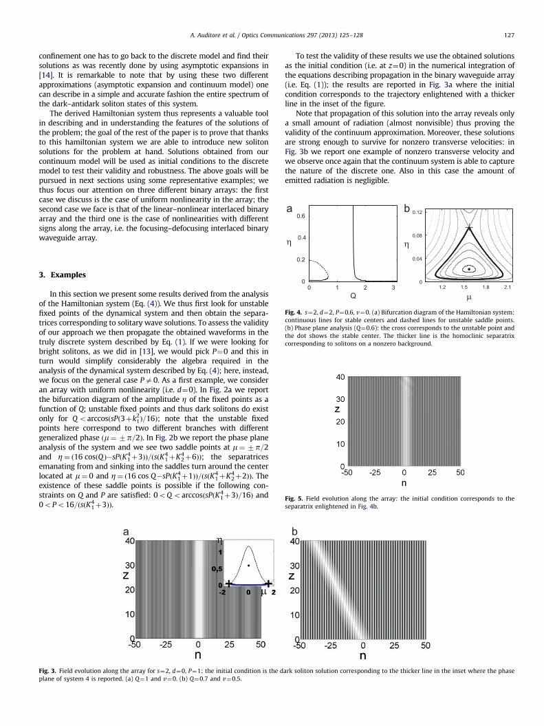
Fig. 3. Field evolution along the array for s¼2, d¼0, P¼1: the initial condition is the d

plane of system 4 is reported. (a) Q¼1 and v¼0. (b) Q¼0.7 and v¼0.5.

To test the validity of these results we use the obtained solutionsas the initial condition (i.e. at z¼0) in the numerical integration ofthe equations describing propagation in the binary waveguide array(i.e. Eq. (1)); the results are reported in Fig. 3a where the initialcondition corresponds to the trajectory enlightened with a thickerline in the inset of the figure.

Note that propagation of this solution into the array reveals onlya small amount of radiation (almost nonvisible) thus proving thevalidity of the continuum approximation. Moreover, these solutionsare strong enough to survive for nonzero transverse velocities: inFig. 3b we report one example of nonzero transverse velocity andwe observe once again that the continuum system is able to capturethe nature of the discrete one. Also in this case the amount ofemitted radiation is negligible.

ark soliton solution corresponding to the thicker line in the inset where the phase

Fig. 7. Field evolution along the array for s¼2, d¼2.1, Q¼1.7, P¼1 and v¼0. The

initial condition corresponds to the separatrix enlightened in Fig. 6b.

0 1 2 30

5

10

15

20

−2 0 2 4 60

1

2

Fig. 6. s¼2, d¼2.1, P¼1.0, v¼0. (a) Bifurcation diagram of the Hamiltonian

system: continuous lines for stable centers and dashed lines for unstable saddle

points. (b) Phase plane analysis (Q¼1.7): the crosses correspond to the unstable

points and the dots show the stable centers. The thicker line is the heteroclinic

separatrix corresponding to solitons on a nonzero background.

A. Auditore et al. / Optics Communications 297 (2013) 125–128128

As a second example we consider the case of an array ofalternating linear–nonlinear waveguides, i.e. s¼d. The situation isquite different with respect to the d¼0 case: two fixed points (onecenter and one saddle) exist for Q op=2 whereas only one stablecenter exists for Q 4p=2 (see Fig. 4a). In Fig. 5 we report the beampropagation along the array using as initial condition the fieldprofiles obtained from Eq. (3) after having solved for the trajectoryalong the separatrix described as a thick line in Fig. 4b. The thirdexample we consider corresponds to an array of alternating focus-ing–defocusing nonlinearities, i.e. d4s (s¼2 and d¼2.1 in whatfollows). As we can see in Fig. 6a, for Q 4p=2 we find one center andone saddle. In the corresponding phase plane in Fig. 6b we report theheteroclinic trajectory emanating from and sinking into the saddlepoints at m¼�p=2 and m¼ 2p�p=2. In Fig. 7 we show the fieldevolution along the array using as initial condition the field profilesobtained from Eq. (3) and corresponding to the separatrix enligh-tened in Fig. 6b. Once again we can observe that propagation of this

solution into the array reveals again a negligible amount of radiationthus proving the validity of our analytical approach.

4. Conclusions

In this work we have obtained dark and antidark solitonsolutions in a binary waveguide array with alternating positiveand negative linear couplings between adjacent waveguides and inthe presence of focusing and/or defocusing Kerr nonlinearity. Thesesolutions do exist also in a linear–nonlinear interlaced array andthey even survive in focusing–defocusing interlaced arrays. We havealso numerically verified the soundness of our approach by adetailed comparison with exact results obtained by numericallysolving the discrete system; remarkably our results, obtained in theframework of a continuum approximation, retain their validity alsofor very strong degrees of localization.

Acknowledgments

The authors wish to thank Professor T.R. Akylas for very helpfuldiscussions. A.A., C.D.A. and M.C. acknowledge financial support fromCARIPLO Foundation under Grant no. 2010-0595 and US ARMYunder Grant no. W911NF-12-1-0202.

References

[1] F. Lederer, G.I. Stegeman, D.N. Christodoulides, G. Assanto, M. Segev,Y. Silberberg, Physics Reports 463 (2008) 1.

[2] S. Longhi, Optics Letters 31 (2006) 1857.[3] M. Guasoni, A. Locatelli, C. De Angelis, Journal of the Optical Society of

America B 25 (2008) 1515.[4] N.K. Efremidis, P. Zhang, Z. Chen, D.N. Christodoulides, C.E. Ruter, Detlef Kip,

Physical Review A 81 (2010) 053817.[5] M. Conforti, M. Guasoni, C. De Angelis, Optics Letters 33 (2008) 2662.[6] M. Guasoni, M. Conforti, C. De Angelis, Optics Communications 283 (2010) 1161.[7] S.H. Nam, E. Ulin-Avila, G. Bartal, X. Zhang, Optics Letters 35 (2010) 1847.[8] C.M. de Sterke, L.C. Botten, A.A. Asatryan, T.P. White, R.C. McPhedran, Optics

Letters 29 (2004) 1384.[9] Y.S. Kivshar, A.A. Sukhorukov, Optical Solitons: From Fibers to Photonic

Crystals, Academic Press, San Diego, 2003.[10] A.A. Sukhorukov, Y.S. Kivshar, Optics Letters 27 (2002) 2112.[11] R. Morandotti, D. Mandelik, Y. Silberberg, J.S. Aitchison, M. Sorel,

D.N. Christodoulides, A.A. Sukhorukov, Y.S. Kivshar, Optics Letters 29 (2004) 2890.[12] A.A. Sukhorukov, Y.S. Kivshar, Optics Letters 30 (2005) 1849.[13] M. Conforti, C. De Angelis, T.R. Akylas, Physical Review A 83 (2011) 043822.[14] M. Conforti, C. De Angelis, T.R. Akylas, A.B. Aceves, Physical Review A 85

(2012) 063836(1–4).[15] A. Marini, A.V. Gorbach, D.V. Skryabin, Optics Letters 35 (2010) 3532.[16] Y.S. Kivshar, Physical Review Letters 70 (1993) 3055.[17] N. Flytzanis, B.A. Malomed, Physics Letters A 227 (1997) 335.[18] K. Hizanidis, Y. Kominis, N.K. Efremidis, Optics Express 22 (2008) 18296.[19] E.W. Laedeke, K.H. Spatschek, S.K. Turitsyn, Physical Review Letters 73 (1994)

1055.[20] A.B. Aceves, S. Wabnitz, Physics Letters A 141 (1989) 37.[21] J. Yang, Journal of Computational Physics 228 (2009) 7007.