Damage modelling of large and small scale composite … and Safety Executive Damage modelling of large and small scale composite panels subjected to a low velocity impact H E Johnson

Health and Safety Executive

Damage modelling of large and small scale composite panels subjected to a low velocity impact

Prepared by the Imperial College and the United States Naval Academy for the Health and Safety Executive 2006

RR520 Research Report



H E Johnson & L A Louca Civil and Environmental Engineering Department Imperial College 47 Prince’s Gate Exhibition Road London SW7 2QA

S E Mouring Department of Naval Architecture and Ocean Engineering United States Naval Academy Annapolis MD 21402 USA

Professor Charles N Calvano, FSNAME, FRINA Office of Naval Research Global Edison House 223 Old Marylebone Road London NW1 5TH

The advantages of using fibre reinforced plastics, composed of glass fibres embedded in a resin mix, for offshore structures and shipbuilding have been recognized for many years. These are seen to include: (a) Reduced weight, (b) Better corrosion resistance, (c) Lower whole life cycle costs, (d) No hot work required for retrofitting and (e) better thermal, acoustic and vibration properties. For naval vessels, they have the added advantages of lower signatures and the elimination of fatigue crack issues between steel decks and composite deckhouses. Despite this, their use on large scale structures as primary members has been restricted in the offshore industry. Naval applications have recently increased form the traditional mine countermeasure vessels to large hangers on destroyers. Many other naval applications are being proposed and a large volume of research is currently being undertaken. One of the drawbacks with composites is the lack of robust damage models applicable to large composite structures capable of reliably predicting damage growth and ultimate failure loads. This is particularly so in the prediction of delamination which can occur when composites are subjected to lateral impact or shock loads. Damage modelling has been studied extensively particularly at the micro and nano scale. The advances made in damage modelling on a meso and macro scale have been attributed largely to the aerospace industry and little work has been carried out to validate their techniques on marine structures. The class of composites, scale of structures and the nature of the loading is very different to that experienced in the aerospace industry.

This report and the work it describes were funded by the Health and Safety Executive (HSE). Its contents, including any opinions and/or conclusions expressed, are those of the authors alone and do not necessarily reflect HSE policy.

HSE Books

© Crown copyright 2006

First published 2006

All rights reserved. No part of this publication may bereproduced, stored in a retrieval system, or transmitted inany form or by any means (electronic, mechanical,photocopying, recording or otherwise) without the priorwritten permission of the copyright owner.

Applications for reproduction should be made in writing to:Licensing Division, Her Majesty’s Stationery Office,St Clements House, 216 Colegate, Norwich NR3 1BQor by email to hmsolicensing@cabinetoffice.x.gsi.gov.uk

ii

EXECUTIVE SUMMARY

Although composite materials have been used for some time in the marine industry such as in the construction of mine countermeasure vessels, surprisingly little work appears to have been performed to gain an understanding of the detailed response to shock loading and the residual strength after a shock load. Delamination damage is a particularly common and serious damage mode resulting from a shock load, and if undetected, can lead to catastrophic failure. The ability to computationally model a structure under a potentially damaging load is increasingly sought after. The marine industry envisages full-scale modeling capabilities of its vessels and the ability to predict damage and survivability after a damaging load.

There is limited development work on in-plane testing, shock testing and damage modeling of large-scale composite structures and little validation of current failure criteria in this area. In addition, the vast proportion of the work is carried out on aerospace composites, which are inherently different to marine composites. In this study, both existing and developed failure criteria are put to the test under quasi-static and dynamic loading of large and small-scale composite plates, in an attempt to effectively capture the response of the plates and obtain an indication of the extent and severity of the damage incurred. The models must be manageable and run under realistic time scales.

The residual strength of a damaged composite plate is vital in assessing its survivability. One method of deriving the residual strength of a panel is to compare the in-plane compressive strength before and after shock loading. Two of the three tests required for this were carried out in the present work: in-plane compression testing of intact panels and impact testing. Impact testing was chosen over UNDEX (under water explosion) testing because of limited access to under-water shock data and publishing restrictions related to this data. Two separate studies were performed.

The first study involved in-plane compression testing and finite element (FE) modeling of large-scale plates. Abaqus/Standard was used with a USFLD (user defined field) subroutine. A parametric study was carried out to assess the effect of various modeling variables, including imperfection size and boundary conditions. Various failure criteria were tested and it was found that the implementation of a modified version of Hashin’s 2d failure criteria predicted the in-plane compression behaviour of the panels seemingly well.

The second study involved low-velocity impact testing of both small-scale and large-scale plates conducted in the U.S.A. and the validation of two different FE models in Abaqus/Explicit. The first model aimed to validate Hashin’s 2d criterion under a dynamic load and to assess the effectiveness of resin-rich layers for delamination. The resin-rich layer technique was moderately successful using a simple energy criterion for failure. The maximum delamination areas were conservatively predicted although not in the correct locations. The second model implemented 3d damage criteria in a VUMAT (user material subroutine) and delamination was modeled using cohesive elements. The contact force and damage predictions were good overall.

The objective to both experimentally assess and model the behaviour of composite plates of various sizes and obtain an indication as to the severity of matrix, fibre and delamination damage, was achieved. The proposed models are intended as points of reference for future model developments. There is vast scope for future work in shock modeling of marine plates. The CAI (compression after impact) tests and simulations were not performed in this study and still need to be addressed. As far as we are aware, the transfer of the damaged (residual) state of a composite structure from Abaqus/Explicit to Abaqus/Implicit has not been attempted, which would be required for a CAI FE

iii

analysis. Mesh independence should also be further looked into, which is a prime consideration when it comes to the development of scale-independent solutions. Coupled with this is the scaling of material properties obtained from small coupon tests. Abaqus software although effective, does have its limitations when it comes to the implementation of user-defined criteria. One of the most significant drawbacks is in the lack of information available in the subroutines on the mesh features, which prevents the proper application of smeared models particularly when the mesh is discontinuous, or coupling of the constitutive materials.

iv

i

1. Introduction 1

2. In-plane compression testing and modelling 5

2.1. Method 5

2.2. Parametric study 10

2.3. Strains and displacements 13

2.4. Conclusion 21

3. Impact modelling – using resin rich layers for delamination 22

3.1. Introduction 22

3.2. Experimental - impact testing 23

3.3. The damage model 25

3.4. Large plates (1.3716x1.3716x0.0381m) 27

3.5. Small plates (0.2286x0.1778x0.00638m) 32

3.5.1. Modelling variables 33

3.5.2. A viscoplastic model at the resin-rich layers 41

3.6. Conclusion 43

4. Impact modelling – using a 3d damage model with cohesive layers 45

4.1. Introduction 45

4.2. The damage model 464.2.1. Damage initiation 47

4.2.2. Damage propagation 48

4.2.2.1. In-plane damage 49

4.2.2.2. Transverse damage 54

4.3. Results and discussion 574.3.1. Small plates (0.2286x0.1778x0.00638m) 57 4.3.2. Large plates (1.07315x0.76835x0.019m) 68

4.4. Conclusion 80

5. Closing comments 81

6. Further development 82

Acknowledgements 84

v

vi

1. INTRODUCTION


1.1. SCOPE OF WORK

The bulk of the project has been funded by the Office of Naval Research (ONR) from the USA as part of their program on improving the understanding of the behaviour of fibre reinforced composite materials subjected to shock loading. The scale of structures involved mean they are also ideal candidates for consideration in offshore applications, and as outlined above, have a number of potential benefits. The methodology for the work undertaken involved a combination of testing and the development of robust analytical models to validate against the experimental data. Developments in damage modelling are not as robust for composite materials as they are in modelling damage to metal structures due to their more complex damage modes and make up exhibiting anisotropic and non-homogeneous behaviour. Composites are also more sensitive to the manufacturing process and in many cases are very dependent on the skill of the individual.

In composite design, the performance of the structural component can be determined through the residual properties that are considered important to the design application. The aerospace industry has an established procedure for dealing with impacts and all parts need to be designed as damage tolerant. This has put into place inspection levels and limit loads. The CAI (compression after impact) is considered a critical design measure. More specifically, certain damage thresholds have been put in place such as assumptions of damage type and size and service life. The naval industry also has stringent performance measurements but these have generally been limited to the full scale use of composites for naval applications. In addition to the requirements imposed on commercial ship structures, Naval structures are required to resist highly dynamic loads during combat situations, due to weapons impact, or to air or underwater explosions. The developments made in the understanding of the damage mechanisms from shock, blast and UNDEX loads on the structural response of ship and

1

submarine structures, have resulted in structural design aimed to alleviate the effects of this type of loading. As far as composite design in the US navy, one of the requirements is that the structure must survive an impact from a 680kg (1500lbs) load travelling at 10 knots (5m/s) i.e. 8500J; a much harsher demand on the material compared to the 133J kinetic energy imposed in aircraft design. Currently there is still a lack of data relating to the survivability of naval composite structures to such dynamic loading (1) and there is no one specific failure criterion to determine failure of a plate under impact damage. The major focus of the ONR is on the establishment of physically based models for deformation and failure.

A few composite damage models have been inbuilt in finite element packages or developed as stand-alone programs, e.g. Williams’s 2d CDM model in LS-Dyna (2). As far as we know, they were all developed for static loading or plane stress conditions. However, there are currently no established failure criteria to effectively model damage or determine full failure of a composite structure under a dynamic load. Non-destructive ways of measuring damage do exist, including visual inspection with a bright light, ultrasound methods, X-radiography, X-ray computed tomography (CT), laser holography and acoustic emission technology. For in-service damage, visual inspection with a bright light, information on the limited available test data and common sense is used to decide whether a component should be repaired or replaced.

The current work examines several methods of modelling damage in woven E-glass/vinyl-ester composite plates using a finite element (FE) package. Attention is placed on repeatability, computational cost and ease of application. This work is part of a wider study by the Office of Naval Research to establish the residual strength of the panels under in-plane compression loading. There are three stages to the work: 1.To obtain the intact strength of a panel; 2. Incurring damage in the panel using a shock load; 3. Obtaining the residual strength after shock loading, see Figure 1. In this study, stages 1 and 2 are completed.

= ( / )

load load

residual strength of intact panel after inplane loading, R1

loss of strength from damage

R1- R2 R1 x100%

residual strength of impact damaged panel after inplane loading, R2

drop weight impact

Figure 1. The three stages of work

The scope of the testing included impact tests of plate specimens at both a large scale to minimize the effect of the boundary conditions on the response and small scale testing where more tests can be performed due to reduced costs. The cost of testing at large scale is expensive as more manpower is involved in setting up each test. The small scale specimens

2

were fairly simple to set up and a more extensive range of parameters was studied. The numerical modelling was performed using a non-linear finite element computer package Abaqus Explicit where a number of subroutines were developed to describe the constitutive behaviour of the materials and the failure modes observed such as matrix cracking, fibre failure and delamination.

1.2. BACKGROUND TO PROBLEM

The need for increased operational performance and reduced costs has driven the development of composite materials for naval structures. Improvements to warships and submarines are sought in numerous areas such as stability, corrosion resistance, payload and resistance to impact and explosive shock, where composite materials are advantageous. Thus the ability to model the damage incurred from a dynamic load is of increased importance.

Commercial FE codes are currently implemented to model impact of composite plates but most still lack effective constitutive models for laminates experiencing damage. Experimental data is also scarce on composites, relating particularly to contact force history, which according to Zhou and Greaves (3) is one way of revealing the dominant damage mechanisms by examining the peaks.

The initiation of damage in composite materials is the point at which the stresses or strains in the material are large enough to incur some permanent deformation in the form of matrix cracking. Stress or strain based criteria have been the most common tools to model failure on a macro-scale but in a basic way, degrading the properties once only down to a residual value. Currently however, continuum damage mechanics (CDM) is becoming increasingly popular but has yet to be introduced in many finite element packages for composites modelling on a macro scale.

Transverse cracks i.e. cracks that run perpendicular to the plies, are created by in-plane stresses and can severely reduce the composite’s stiffness. These can also create in-plane cracks between the plies more commonly referred to as delamination damage. The damage incurred from shock loading of a composite panel takes the predominant form of matrix cracking and delamination, followed by fibre failure if the peak over-pressure is large enough. Delamination is sometimes difficult to detect when the material is in service. It can be quite extensive, internal and often undetectable with the naked eye and it’s effect often deceiving as the composite structure can often survive the impact/blast and maintain its integrity even if severely reducing its strength. Delamination therefore becomes the most concerning and destructive failure mode. One simple method of modelling delamination involves the implementation of resin-rich layers. These have been discussed by Elder (4) as a method of modelling delamination damage and were tested by Boh (5) giving good results. However, they do not model the physical separation and ensuing contact condition of the delaminated layers. It is evident that to effectively model and thus the reduction in contact force, cohesive elements are an attractive option. Cohesive elements are used by authors such as Espinosa (6) , Chen (7), Scheider (8), Camanho (9), and Turon (10). More recently and more specific to naval composites, Lemmen et al (11) proposed a damage mechanics based model for quasi-static loading of a T-joint panel using a coupled mode I and II linear traction-separation cohesive zone model for delamination and used a damage initiation criterion based on Hashin’s work (12). The model was tested for the quasi-static loading of a T-joint panel and compared with experiment.

3

In this study, the majority of the tests were carried out on laminated made from E-glass/Dow Derakane 8084 vinyl-ester, manufactured by an advanced Vacuum Assisted Resin Transfer Moulding (VARTM) technique called ‘CARTM’ (Channel Assisted Resin Transfer Moulding), whose average properties are shown in Table 1.

E11 E22 E12 S13 /MPa S23 /MPa /GPa /GPa /GPa 24.139 24.139 8.273 51.6 51.6 E13 E23 S11T (warp) /MPa S22T S11c=S22c /GPa /GPa (fill) /MPa /MPa 3.585 3.585 330.328 298.6 329.6

Table 1. Average material properties for the E-glass/Derakane 8084 vinyl-ester

4

2. IN-PLANE COMPRESSION TESTING AND MODELLING

2.1. METHOD

This study was aimed to find the strength to failure of large woven composite panels and compare the results with finite element analyses. The tests performed were able to demonstrate the renowned sensitivity of panels to boundary conditions, which was also reflected in a parametric study carried out in Abaqus/Standard. Two dimensional stress-based failure criteria were implemented via a user-defined field (USFLD) subroutine to detect matrix and fibre damage which allowed progressive damage to be modeled.

The reduction of the material’s stiffness and strength caused by delamination damage is most prominent under in-plane loading, that is when a load is applied parallel to the delaminated layers (13). Obtaining the strength of an intact panel is a method of obtaining the loss in strength of a panel subjected to CAI (compression after impact).

A rig was custom-built to support a panel size of dimensions 1.219x0.9144x0.019m (4ft x 3ft x 0.75in) under simply supported boundary conditions, see Figure 2. The load was applied under displacement control across the 0.9144m wide edge of the panel. A non-linear elastic finite element (FE) analysis in Abaqus/Standard was used to model the experimental tests and damage was determined using the simple 2D Hashin failure criteria (7). Stress based failure criteria, although limited, have been widely used to model either mixed or individual failure modes, many of which were evaluated by Padhi et al (8). A parametric study was carried out to examine the sensitivity of the FE models to changes in boundary conditions, loading type ( )load or displacement control and material properties.

(a) (b)

Figure 2. (a) Panel test 2, (b) Configuration with top roller (side view) used in subsequent tests

5

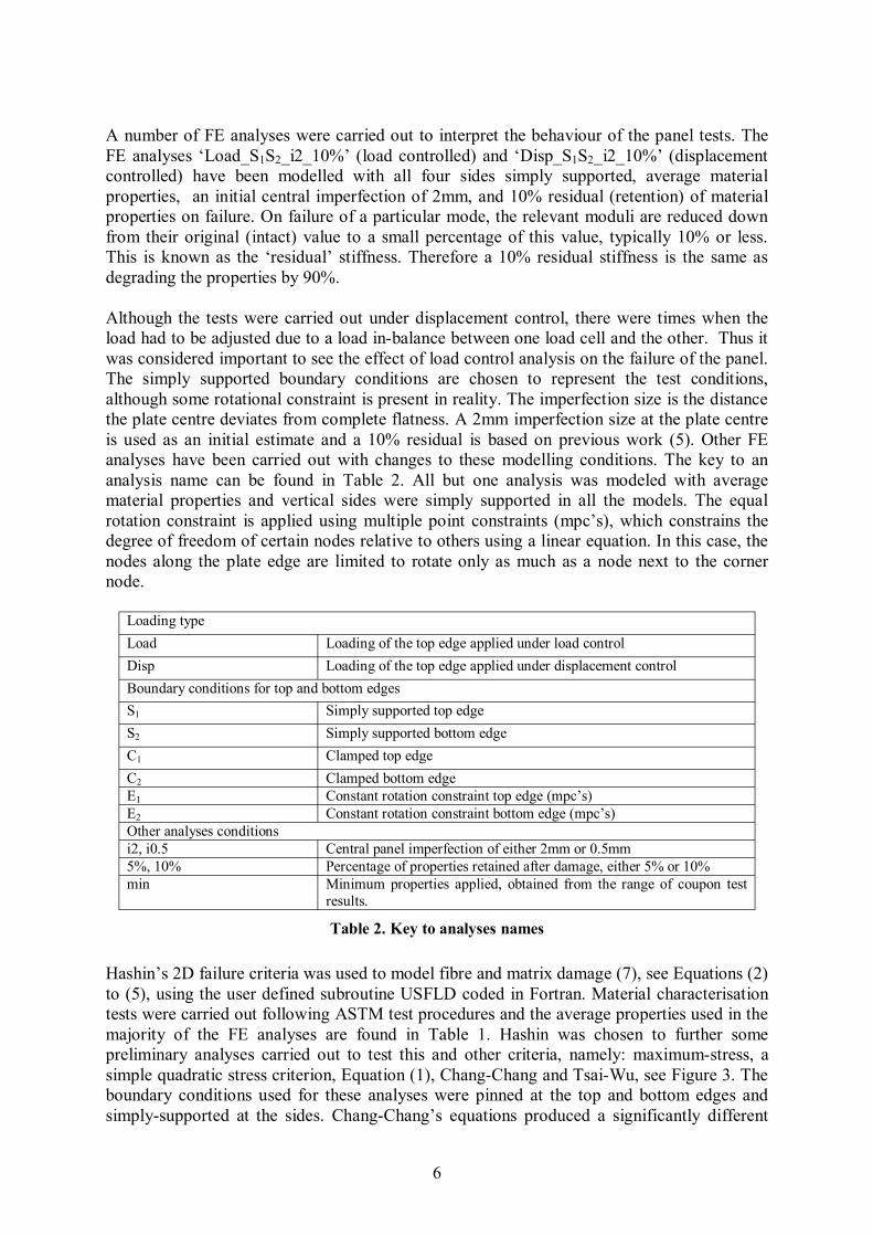
A number of FE analyses were carried out to interpret the behaviour of the panel tests. The FE analyses ‘Load_S1S2_i2_10%’ (load controlled) and ‘Disp_S1S2_i2_10%’ (displacement controlled) have been modelled with all four sides simply supported, average material properties, an initial central imperfection of 2mm, and 10% residual (retention) of material properties on failure. On failure of a particular mode, the relevant moduli are reduced down from their original (intact) value to a small percentage of this value, typically 10% or less. This is known as the ‘residual’ stiffness. Therefore a 10% residual stiffness is the same as degrading the properties by 90%.

Although the tests were carried out under displacement control, there were times when the load had to be adjusted due to a load in-balance between one load cell and the other. Thus it was considered important to see the effect of load control analysis on the failure of the panel. The simply supported boundary conditions are chosen to represent the test conditions, although some rotational constraint is present in reality. The imperfection size is the distance the plate centre deviates from complete flatness. A 2mm imperfection size at the plate centre is used as an initial estimate and a 10% residual is based on previous work (5). Other FE analyses have been carried out with changes to these modelling conditions. The key to an analysis name can be found in Table 2. All but one analysis was modeled with average material properties and vertical sides were simply supported in all the models. The equal rotation constraint is applied using multiple point constraints (mpc’s), which constrains the degree of freedom of certain nodes relative to others using a linear equation. In this case, the nodes along the plate edge are limited to rotate only as much as a node next to the corner node.

Loading type Load Loading of the top edge applied under load control Disp Loading of the top edge applied under displacement control Boundary conditions for top and bottom edges S1 Simply supported top edge S2 Simply supported bottom edge C1 Clamped top edge C2 Clamped bottom edge E1 Constant rotation constraint top edge (mpc’s) E2 Constant rotation constraint bottom edge (mpc’s) Other analyses conditions i2, i0.5 Central panel imperfection of either 2mm or 0.5mm 5%, 10% Percentage of properties retained after damage, either 5% or 10% min Minimum properties applied, obtained from the range of coupon test

results.

Table 2. Key to analyses names

Hashin’s 2D failure criteria was used to model fibre and matrix damage (7), see Equations (2) to (5), using the user defined subroutine USFLD coded in Fortran. Material characterisation tests were carried out following ASTM test procedures and the average properties used in the majority of the FE analyses are found in Table 1. Hashin was chosen to further some preliminary analyses carried out to test this and other criteria, namely: maximum-stress, a simple quadratic stress criterion, Equation (1), Chang-Chang and Tsai-Wu, see Figure 3. The boundary conditions used for these analyses were pinned at the top and bottom edges and simply-supported at the sides. Chang-Chang’s equations produced a significantly different

6

result from Hashin’s due to the shear term in the fibre compression failure equation, not present in Hashin’s equations. The maximum stress criterion is not conservative enough, and by the time any drop in load has occurred due to damage, the peak load attained is already very large compared to experiment, thus the analysis was stopped. With Tsai-Wu, some material degradation takes place after 3.5msecs, but a higher peak force is reached and the analysis was stopped shortly after the peak force. Modelling no damage, but including geometric non-linearity leads to the un-realistically large load-displacement curve, as seen in Figure 4, unable to show a drop in load due to failure. The pictures of damage shown were predicted for the top, tensile ply of the plates.

Although Hashin’s 2 criteria proved to be the most effective at modeling the in-plane compression damage of the composite panels, the load-displacement curves are not the correct shape during the damage phase. It was found that they predicted too large a drop in load once damage initiated regardless of the boundary conditions, material properties, residual load or initial imperfection. Figure 5 highlights this fact with predictions using Hashin’s full equations and three different boundary conditions: simply supported (S1S2), no rotation at the top edge (C1S2) and equal rotation for all points along the top edge (E1S2). Instead, it was found that excluding the separate shear term in the equation to give Equation (6) gives a load/displacement curve that does not droop towards the peak load, thus producing a good correlation with experiment, see ‘Hashin_S1_S2’ plot. In contrast, removing the shear term from the equation for fibre damage in tension made negligible difference to the damage prediction and load/displacement curve, as highlighted with a circle on the graph.

2 2 σij 2

∑∑ ≥ 1 (1)i 1 i 1 Sij = =

Where Sij is the strength of the material in the direction ij

7

Figure 3. Comparison of various failure criteria.

Figure 4. Demonstrating the importance of modeling damage

8

2 2 σ11 (2)

+ σ12

≥1 XT S12 2d Hashin - Fibre tension failure

σ11C ≥1 (3)XC

2d Hashin - fibre compression failure 2 2

σ 22 (4)

+ σ12

≥1 YT S12 2d Hashin - matrix tension failure

σ 2

22 YC

2 σ22 2

σ12

≥ 1 (5)

1 − + + YC 2S12 2S12 S12 2d Hashin - matrix compression failure

2σ22

YC 2

− + σ22 ≥ 1

(6) 1 YC 2S12 2S12

Figure 5. The effect of removing the shear term in Hashin’s equations and various boundary conditions.

Based on the above, the ensuing analyses, unless otherwise specified, applies this modified version of Hashin’s 2d criteria, i.e. the implementation of Equations (2), (3), (4) and (6).

9

The buckling loads obtained from experiment show a scatter of up to 25%. However, there is only a 3% difference between the average buckling load for panel tests 1 to 5 in Table 3 and the buckling load from the FE analysis which models a simply supported panel, see Table 4.

FE – simply supported.1

FE – equal rotation constraint. 2

FEclamped topbottom. 3

–

&

Theory: simply supported.4

474.52 kN 681.1 kN 747.2 kN 441.9 kN 1. From analyses: load_S1S2_i2_10% and Disp_S1S2_i2_10% 2. From analyses: Load_E1E2_i2_10% and Disp_E1E2_i2_10% 3. From analyses: Load_C1C2_i2_10% and Disp_C1C2_i2_10% 4. E.Greene

Table 3. Experimental critical Table 4. FE and theoretical critical buckling loads buckling loads

Theoretical buckle loads were also compared. An analytical expression which takes into account the orthotropy of a laminate is that by Eric Greene (14), whose work uniquely addresses large composite structures for the marine industry.

2.2. PARAMETRIC STUDY

A parametric study in Abaqus/Standard was carried out to see the effect of boundary conditions, residual stiffness, initial imperfection and material properties. The results are here summarized.

Boundary conditions: The sensitivity to boundary conditions in the FE analyses is the same for both load and displacement control analyses. Figure 6 shows the effect of reducing the mobility of the top and bottom horizontal plate edges. The analyses shown were all carried out under load control with a 2mm central imperfection and 10% residual stiffness. Preventing rotation of the edges by assigning clamped conditions, ‘C1C2’ for both edges produces the greatest pre- and post-buckling stiffness. Clamping the top edge over the bottom edges in ‘C1S2’ reduces the fold that is created at the top of the plate and thus reduces the damage development concentration in the top half of the plate, thus producing a higher residual strength.

Test number Buckle load (kN) Test 1 440 Test 2 440 Test 3 540 Test 4 460 Test 5 580

10

Figure 6. Sensitivity to bc’s, load controlled FE analyses

Residual stiffness: The effect of applying a residual of 5% or 10% has a significant effect on the predicted residual strength of the panel. This is shown in Figure 7 for a displacement controlled analysis, the same effect also experienced with a load controlled analysis. The residual capacity of the plate is measured just after the plate has suffered global failure, when a significant drop in load is seen for a minor change in deflection. Thus the red lines shown in Figure 7 are indicative of the residual loads for the two analyses.

Figure 7. Sensitivity to residual stiffness, load and displacement controlled FE analyses

11

Initial imperfection: The increase in initial imperfection at the centre of the plate from 0.5mm to 2mm (i0.5, i1 and i2) is shown with a reduction in pre-buckling stiffness and buckling load, seen in Figure 8. The figure also demonstrates how for the same residual stiffness (10%), the peak strength and particularly the residual strength of the displacement controlled analysis is considerably higher than for the load controlled equivalent.

Figure 8. Effect of initial imperfection.

Material properties: Material properties obtained from a batch of coupon tests showed a 20% scatter. A load controlled analysis with a 2% imperfection and a displacement controlled analysis with a 1% imperfection were carried out using maximum and minimum material properties from the range. Both models implemented a 10% residual stiffness. The variation in material properties has a slight effect on the buckling load but little effect on the post-buckling stiffness, as shown in Figure 7. The peak stress is marginally increased when the maximum properties are implemented, however the residual strength is negligibly affected.

Figure 9. Sensitivity to material properties, load and displacement control FE analyses

12

2.3. STRAINS AND DISPLACEMENTS

As expected, given the aspect ratio of the panel and the designated experimental boundary conditions, all the panels buckled into one half wave-lengths. For simplicity, the plots of o.o.p (out-of-plane) deflections will be restricted to the panel centre, displacement ‘U3’. The load displacement plots for the five panel tests are shown in Figure 3. Acceptable residual loads were only obtained for the panels in tests 3, 4, and 5.

Figure 10. Out of plane displacement at the panel centre versus load for tests 1 to 5

Strain gauges were placed across the whole of the plate at 8 horizontal and vertical locations on both sides for test 2, see Figure 11(a) & (b). For tests 3 to 5 strain gauges were located only on the top quarter of the plate on both sides, as shown in Figure 11(b). The gauges are labeled alphabetically, with single alphabet labeling for the tensile face and double labeling on the compressive face as shown. Panels with lower failure loads are associated with lower strains, seen in Figure 12 and Figure 13 for gauge locations a, c, aa and cc, and smaller o.o.p displacements, seen in Figure 10. Test 2 also had strain gauges at locations ‘e’ and ‘ee’, and these are plotted against the readings at ‘a’ and ‘aa’ in Figure 14.

13

(a) Test 2 (b) Tests 3,4 & 5

Figure 11. Strain gauge locations for tests 2 to 5. The face in compression has gauges labeled with double letters, shown in brackets.

Figure 12. Panel test 2, 3, 4 & 5 strains at locations ‘a’ and ‘aa’.

14

Figure 13. Panel test 2, 3, 4 & 5 strains at locations ‘c’ and ‘cc’.

Figure 14. Panel test 2 strains at locations ‘a’, ‘aa’, ‘e’ and ‘ee’.

All the tests to varying degrees resembled the load controlled FE analysis, ‘Load_S1S2_i2_10%’ in Figure 15, which assumed no rotational constraints. The figure also shows how reducing the mobility of the loaded edges can create stiffness in the post-buckling as well as pre-buckling stages and causes changes to the peak load. Differences in imperfection size during the pre-buckling stages could be misinterpreted as changes in boundary conditions and vice versa, as demonstrated with Figure 6 and Figure 8 in the above parametric study.

15

Panel test 2 gave the larger displacement and strain plots out of all the tests with failure occurring along the top edge whilst the rest of the panel appeared to be undamaged. The rotation along the top edge appeared to be constrained in the last 400kN before the peak load, but the buckling load was the lowest obtained from all the tests, as shown in Table 3. The strains along the top of the panel in test 2 at locations ‘a’, ‘c’ and ‘e’, seen in Figure 16, are similar in magnitude to those of the Disp_S1S2_i2_5% analysis. The strains at ‘a’ and ‘e’ were close to being equal, as also shown more clearly in Figure 14, partly indicating an even load distribution. The strain at ‘c’ is smaller than that at locations ‘a’ or ‘e’, contrary to the other tests where the strain at ‘c’ is larger than at ‘a’. During the early loading stage of tests 2 to 5 it was difficult to maintain the load equal for load cells 1 and 2 under the displacement controlled loading and some load adjustments had to be made.

Figure 15. The most representative FE models of the actual test conditions

16

Figure 16. Comparison of panel test 2 and FE analysis ‘Disp_S1S2_i2_5%’ strains at locations a, c and e

The damage incurred to the panel in test 2 was localized in the two top corners, propagating from each of these corners and along the top edge. The damage was a mixture of matrix cracking, delamination and fibre failure.

For tests following test 2, a 300mm high steel block was introduced between the load cell and the top fixture in an attempt to further improve the load distribution across the panel and remove the localized damage to the top edge. The panel in test 3 failed at nearly an identical load as that predicted by the ‘Load_S1S2_i2_10%’ FE analysis but at a slightly lower central o.o.p deflection. During the buckling stage the panel was very stiff, giving the second highest buckling load out of the five tests. This panel appeared to be flatter than all the other panels and its buckling direction was not clear, demonstrated after the first 300kN or so of loading through a very noticeable change in direction of the central o.o.p displacement, as shown in Figure 10. This panel failed at the top corners, with cracking and delamination for one corner attempting to propagate in a direction that was about 30° from the top edge. The damage to the other corner propagated along part of the top edge similar to panel test 2. The high stiffness at the start may appear to resemble the FE analysis for clamped top and bottom edges, however the tested panel is not as stiff in the post-buckling region and its buckling load is smaller, as can be seen in Figure 15. Its behaviour is clearly much closer to the analysis with the smaller imperfection size of 0.5%: Load_S1S2_i0.5_10%, illustrating that the initial stiffness of the panel in test 3 was likely to be dominated by the imperfection size and not the boundary conditions. The strains at the top of the panel in test 3, seen in Figure 17, are actually closer in behaviour to those the simply supported conditions of Disp_S1S2_i2_5% and Load_S1S2_i2_10% analyses, although smaller in magnitude.

17

Figure 17. Comparison of panel test 3 and FE analysis ‘Disp_S1S2_i2_5%’ and ‘Load_ S1S2_i2_10% ‘strains at locations ‘a’, ‘aa’. ‘c’ and ‘cc’.

For test 4 and test 5, rubber strips were inserted between the knife edges and the panel and the knife edges were moved inwards by a total of 20mm to alleviate any rotation constraint at the corners. The panel in test 5 also had the corners chamfered by 40mm to further reduce the stress concentrations at these corners. The top and bottom roller of the panel in test 4 stopped rotating a couple of loading increments prior to failure, which caused the entire 300mm steel block to rotate off axis by a couple of degrees. Examination of the damage, again was found exclusively at the top of the panel, as seen in Figure 18 for test 4. The panel in test 5 behaved similarly to that of test 4 but failed at the lowest load of about 950kN. The strains at the top of panel test 3,4 and 5 follow a similar trend as seen in Figure 12, with the top-centre strains at ‘c’ being larger than those nearer the corners at ‘a’. This trend appears to reflect a resemblance towards the load-controlled analyses generated by with the FE analyses (even though the testing was displacement controlled).

18

Figure 18. Panel test 4 – showing final failure pattern

The FE analysis Disp_E1E2_i2_5% in Figure 15 models uniform in-plane deflection and rotation along the top edge to reflect the idealized test conditions. In all the tests, the panels buckle into a half wave length in both directions giving the maximum o.o.p deflection at the centre of the panel. This however changes as the peak load is approached, and the maximum o.o.p displacement starts to migrate towards the top of the panel. The Load_S1S2_i2_10% analysis, having no rotation constraint, exaggerates this behaviour with the creation of a prominent ‘fold’ at the top edge and giving rise to higher strains in the top third of the panel. In contrast, the matrix cracking, delamination and fibre failure patterns in all the panels either form or attempt to form the damage simulated in the Load_E1E2_i2_10% and Disp_E1C2_i2_5% analyses shown in Figure 19 and Figure 20. The damage predicted with Load_ S1S2_i2_10% is similar except that fibre damage does not initiate at the corners but initiates at the ‘fold’. Judging by the results and stiffness effects caused by dissimilar imperfections between panels, the panels are probably being supported as intended during the buckling stages. However subsequently, during the early post-buckling stages with increase in load, one of the rollers appears to stick intermittently which can lead to out-of-plane movement of the 300mm loading block and consequently sudden premature failure. Some movement within the resin may also be occurring during these stages causing the stiffness of the curve in the post-buckling regime to fall slightly. The test may therefore be providing imperfect boundary conditions. The panel in test 2 resisted a higher load probably because the rotation at the top of the plate was taking place at the roller bearings within the load cells and not at the less sophisticated full length roller used in tests 3 to 5. In summary, the behaviour of the panels is reflected in the following FE analyses, independent of the imperfection size and residual load: Load_S1S2, Load_E1E2, Disp_E1E2 and Disp_E1C2 in Figure 15. The main difference between the FE load controlled analyses compared to the displacement controlled analyses is in the poorer stress distribution and thus the lower peak load. The even load distribution that would have been achieved with a perfect displacement controlled analysis was not obtained. Thus, the test loads are closer to the load controlled analysis peak loads. Although it is likely that the boundary conditions were not perfectly consistent, the shape of the displacement/load graphs are still of closer resemblance to the simply supported boundary conditions than the simply supported conditions with rotational control (E1E2)

19

(a) (b) (c)

Figure 19. Load_ E1E2_i2_10% FE results for the top ply (tensile face) at the end of the analysis, showing (a) matrix cracking, (b) fibre failure, (c) o.o.p displacement

(a) (b) (c)

Figure 20. Disp_E1C2_i2_5% FE results for the top ply (tensile face) at the end of the analysis, showing (a) matrix failure, (b) fibre failure, (c) o.o.p displacement

For tests 3 to5, the longitudinal strains measured at the panel centre reflect the movement of the tensile face from an initial state of compression during the pre-buckling stages to a state of tension thereafter. The exact reverse can be said about the compression face, as see in Figure 21. This reinforces the uncertainty of the panels to deflect in one direction or another. The initial compressive strains seen on the tension face are larger than the initial tensile strains on the compression face which is explainable because the loading is in compression.

20

Figure 21. Longitudinal centre panel strains from tests 1 to 4, and FE analyses Disp_S1S2_i2_10% and Load_S1S2_i2_10%

2.4. CONCLUSION

It is evident from the five panel tests that the load was largely more distributed across the top half of the panels and consequently not generating any visible damage on the bottom half. This was possibly due to the slight difference in stiffness at the top of the rig compared to the bottom. The in-plane domination of such a compression test suggests that the non-linear FE analyses, using the simple 2D Hashin stress-based criteria, can effectively model the panel’s response. The study has highlighted the sensitivity of the FE analyses to different variables and also the sensitivity of the test procedure and boundary conditions. Symmetry of the applied load, friction at the boundaries, boundary conditions and differences in panel initial imperfections have shown to contribute greatly to pre-buckling and post-buckling stiffness and maximum load carrying capacity. There is no individual FE model discussed above that can fully replicate the panel tests unless the test conditions are assumed to be ideal or the exact conditions can be pin-pointed. However, one panel test can show similarities in behaviour to a combination of FE models. The FE analyses cannot be assumed to be correct in their predictions but they do provide good representations of the behaviour of the tested panels. The panel tests have been valuable and have provided an indication of the panel behaviour and strength of which little data has been previously reported in the public domain.

21

3. IMPACT MODELLING – USING RESIN RICH LAYERS FOR DELAMINATION

3.1. INTRODUCTION

The main concern in this study was to model the underlying delamination damage at the interlaminar regions using full-scale data. Three delamination criteria are tested: two simple stress criteria and an energy approach. Hashin’s 2D stress criterion is used to model matrix and fibre failure. The criteria for delamination are applied at resin-rich layers (RR-layers), these being a resin-rich region that is naturally present in between every ply in composite materials and it is at these locations that delamination is most likely to occur. Although the use of RR-layers is still a relatively new and under-practiced technique, literature suggests that a maximum transverse shear strain criterion has been previously applied at the RR-layers to model delamination, (15). Other work includes that by Boh et al (5) who applied a maximum stress criterion at the RR-layers in modelling the response of woven composite beams subjected to transverse shear loading.

Delamination is a very prominent failure mode for shock damaged composites and should ideally be modeled using full scale test data to minimize any scaling uncertainties (16). For low velocity impacts the delamination and matrix damage area is proportional to the impact energy, (17). In order to validate the numerical model, both large and small scale panels, have been shocked under impact. The sensitivity of the results to two modelling variables is examined, particularly with respect to the transverse stress predictions.

FE analyses are carried out in Abaqus/Explicit to model the low velocity impact of two different sized plates in order to calibrate the models at different scales. The large scale panel measures 1.524x1.524x0.0381m (5x5ftx1.5in) and the small scale panels are 0.2286x0.1778x0.00638m (9x7x0.25in).

Strain rate tests on vinyl-ester composites have indicated an increase in modulus and strength values over those from quasi-static tests, (18). Strain rate tests in the warp and fill directions of a SCRIMP manufactured glass/vinyl-ester 510A WR were carried out for strain rates ranging from 0.1 to 5/s, (19). However the available high-strain rate through-thickness data available was carried out under compression only on a poorly consolidated hand lay-up glass/ Derakane 8084 composite sample obtained from a half-scale Corvette, subjected to strain rates of 0.001s-1 and 100s-1. The composite was giving results that are smaller than was what obtained under quasi-static loading for a very similar resin, a Derakane 510A, manufactured by the superior SCRIMP process, whose results seen in Table 5 are thus used in the present study.

22

Material Average ultimate strength / 106N/m2 Average modulus of Elasticity / 109N/m2

Resin Batch 1 Panel #1 FVF=52.3%

Tens.: 35.43 STD = 2.4

Tens.:10.27

Comp.: 541.55 STD = 21.11

Comp.:12.44


Tens.: 33.95 STD = 2.97

Tens.:12.08

Comp.:563.78 STD = 28.19

Comp.:14.08


Tens.: 21.36 STD = 2.59

Tens.: 11.17

Comp.: 547.41 STD = 36.67

Comp.:13.62


Tens.: 39.66 STD = 2.06

Tens.: 11.08

Comp.: 547.18 STD =9.18

Comp.: 14.46


Tens.: 22.17 STD = 1.9

Tens.: 12.66

Comp.: 591.71 STD = 12.47

Comp.: 17.65

Table 5. Through-thickness tensile and compressive strengths and moduli taken from 5 panels fabricated from E-glass and Dow D

The main concern in this study is to model the underlying delamination damage at the interlaminar regions. A simple energy approach is used to model delamination and Hashin’s 2D stress criterion to model matrix and fibre failure. The energy criterion for delamination is applied at the resin-rich layers (RR-layers), these being a resin-rich region that is naturally present in between every ply in composite materials and it is at these locations that delamination is most likely to occur.

Delamination is a very prominent failure mode for shock damaged composites and should ideally be modeled using full scale test data to minimize any scaling uncertainties. For low velocity impacts the delamination and matrix damage area is proportional to the impact energy, (15). In order to validate the numerical model, both large and small scale panels have been shocked under impact. The sensitivity of the results to two modelling variables is examined, including damage criteria, element type and mesh density.

3.2. EXPERIMENTAL - IMPACT TESTING

In order to incur the kind of damage that would be produced by a vessel impacting debris at sea (such as logs) under a speed of up to 10 knots, (5.1 m/s) the impactor must be heavy, of large diameter and travel at a low velocity. A schematic of the large panel test fixture is shown in Figure 22. Following smaller impact trials, the tup mass was chosen as 453kg (1000lbs), the tup diameter 203mm (8in) and the tup velocity 4.6 ms-1 (15ft/s).

The small plates were tested using an Instron-Dynatup Model 9250HV (High Velocity) Impact Test Instrument with Impulse Control and Data System shown in Figure 23. Two tup diameters were used to impact the panels: a 25.4mm (1inch) and a 38mm (1.5inch) hemispherical tup. These were dropped under gravity to impact at a velocity of 4.6m/s. A photodiode was used to determine the velocity of the impactor just before impact. The high

23

speed video was taken using an Olympus I Speed mounted on a tripod and recording took place at 1000 frames per second out of a possible 33000 frames per second.

The small plates fabricated at the Naval Surface Warfare Center (NSWC), Carderock Division using a proprietary 24oz/yd2 woven roving E-glass/Dow Derakane 8084 vinyl-ester manufactured with a vacuum assisted resin transfer molding (VARTM) process. Woven roving reinforcements consist of bundles of continuous strands in a plain weave pattern with more material in the direction of the warp. The large-scale panel was made from 50oz/yd2

WR E-glass/BFG-281/C055 vinyl-ester.

~1.5m

Figure 22. Schematic of large panel impact test fixture

Figure 23. Photograph of the impact test rig

24

3.3. THE DAMAGE MODEL

A User Material subroutine (VUMAT) is needed for all the Abaqus/Explicit analyses if failure criteria are to be defined, forcing the user to also define the composite’s constitutive behaviour. In contrast, Abaqus/Standard allows the option of using a specific User Defined Field subroutine (USDFLD) that allows state dependent variables and user defined fields to describe the failure criteria, omitting the need to write the constitutive equations.

For all of the analyses in this study the RR-layers and the woven plies are modeled an elastic materials that are also elastic damaging. The composite woven plies are orthotropic, and Hashin’s 2D failure criteria are applied at these layers to model matrix and fibre failure. When failure is depicted, the relevant material properties are degraded to 90% of their original value. The transverse shear stiffness and the through-thickness modulus and Poisson’s ratio is only made available in the input file and cannot be modified during the analysis. Delamination damage is modeled with RR-layers, as shown in Figure 24. The RR-layers are modeled as a fraction of the woven ply thickness, typically 5%, reducing the woven layer thickness accordingly to keep the overall laminate thickness constant.

Two types of RR-layer models are examined with the large plate impact simulations. The first model applies a simple in-plane stress criterion at the RR-layers, ‘stress criterion 1’, shown in Equations (7), with the criteria that failure occurs when RRL1 + RRL2 ≥ 1, at which point all the properties of the resin are degraded to nearly zero. A variation of stress criterion 1 is ‘stress criterion 2’, here also evaluated, indicating failure when the largest of either RRL1 or RRL2 is equal or greater than one. The maximum strength values of the resin used in the equations are also reduced to half their value if either matrix or fibre failure is detected first using Hashin’s 2D failure criteria. The strength of the resin in the two in-plane

C C T Tdirections x and y, is denoted by XR and YR for compression and XR and YR for tension.

The second RR-layer model is to apply a simple internal energy failure criterion at the resin rich layers. Two energy density values are compared: the average critical energy density value obtained from typical Mode I fracture tests, see Equation (9), and an energy density criterion from full impact tests.

Figure 24. Composite layering through the thickness of the elements.

25

2C σ11 If σ < 0 then RRL1 = C 11 XR

2T σ11 If σ > 0 then RRL1 = T 11 XR

2C σ22 If σ < 0 then RRL2 = YR

C 22 (7)

2T σ22 If σ > 0 then RRL2 = YR

T 22

Stress criterion 1: RR-layer integration point failure if RRL1 + RRL2 ≥ 1 Stress criterion 2: RR-layer integration point failure if RRL1 or RRL2 ≥ 1

The internal energy per unit mass is calculated at every RR-layer integration point using Equation (8), see Figure 25. When using shell elements, the transverse stresses are not fed into the subroutine therefore only in-plane stresses are used in this equation. This energy value is updated at the end of every time increment and is compared with the critical energy for failure. Ve is the volume of the resin layer for one element width and ρ is the density of the resin.

Eint = 1 1 ε T E ε ∂ V = [ ]{ } (8)∫ 2 { } [ ]{ } 21 ρ

σ ε ρVe Ve

The energy values from the critical fracture tests on the WR E-glass/Derakane 8084 vinyl-ester is shown in Table 6, calculated using Equation (9), where ‘R’ is the thickness of the RR-layer.

Crack initiation Crack propagation

Min value: 3.4in-lb/in2 Min value: 9.05in-lb/in2

(596J/m2) (1665J/m2) Max value:4.6in- Max value: 11in-lb/in2

2lb/in2(806J/m ) (1928J/m2)

Table 6. Mode I critical fracture energy test values for WR E-glass/Derakane 8084 vinyl-ester.

frac E = 1 2 c

el

L L G M

= 1 2

1 2

cL L G L L R ρ

= cG Rρ (9)

The energy value for failure from the impact tests has been obtained from a simple expression, Equation (10), for the total energy absorbed during impact.

26

∂E = ∫tf Pv t (10)t0

Where P and v are the instantaneous load and velocity respectively, t0 is the time of initial impact, taken as zero, and tf is the time at which contact with the plate is lost. Because the instantaneous velocity can only be measured at the beginning and at the end of the impact, the apparent energy can be used instead, as shown with Equation (11).

∂Ea = v0 P t (11)∫0tf

This energy for failure is then divided by the mass of the plate to give an energy value that compares with the internal energy calculated at each integration point.

In these impact tests, the contact force is known from experiment and is used in the apparent energy equation. Where the contact force and time to impact is unknown, an independent energy formulation is required. The ideal is to obtain a critical energy value based on the kinetic energy of the tup which can be applied to a range of plate sizes. The information on the tup mass and impact velocity is more readily available than the contact force and it would be beneficial that the FE model could incorporate this. If the impulsive event comes from a shock wave, such as from an underwater blast, then the blast pressure would be the most likely data resource. Knowing the blast pressure, Equation (11) would then be an appropriate equation to use, where P is the blast pressure.

For both RR-layer models, the resin properties at the integration points are degraded to nearly zero when the failure criteria are met. A small residual is retained for numerical stability.

L1

L2

( )

Thickness of RR-layer

Element-RR-layer Not to scale

integration point

Figure 25. Showing one of the 49 resin-rich layers within an element.

3.4. LARGE PLATES (1.3716X1.3716X0.0381M)

The FE simulation results for the large panel are shown for a single mesh density of 44x44 elements and one element through the thickness. This panel is modeled with 50 composite orthotropic (woven) plies and 49 RR-layers.

The implicit analyses are carried out here using standard thick shell elements, S4R, whereas Abaqus’s SC8R continuum shell elements are tested in the Explicit analyses. Both shell

27

33

element types can model the change in shell thickness and enforce plane-stress conditions, however the S4R use Poisson’s ratio to allow the thickness to change as a function of the membrane strains only. The thickness strain is defined in terms of the in-plane strains, as shown with Equation (12). This equation is then expressed in terms of the equivalent changes in displacement of the element’s reference surface, thus providing an expression for the change in the element thickness. In contrast, the continuum shell elements discretise a three-dimensional body giving them advantages over the conventional shells by modelling the through-thickness response of the shell more accurately. The SC8R calculates two strains: the primary strain is the effective thickness strain at the element centre directly from the element nodal displacements. The secondary strain is obtained under plane-stress conditions by specifying the thickness Poisson’s ratio and allowing the through-thickness strain to be calculated as a linear function of the membrane strains, as with the ordinary thick shells. These secondary strains are subtracted from the primary strains to give the effective thickness strains. An elastic modulus (E33) is defined under the shell section definition in the Abaqus input file and an effective section Poisson’s ratio, making them available during the preprocessing stage of input. The normal stress in the thickness direction is thus obtained using these effective thickness strains and section properties and it is assumed to be constant through the thickness of the element. This average transverse normal section stress can be outputted as SSAVG6 for the shell section; for each element through the thickness. Another advantage of the SC8R over the S4R elements is their superior contact modelling (20).

−νε = (ε + ε 22 ) (12)1 − ν 11

A summary of some of the Standard and Explicit FE results are shown in Table 7. We can see that the most effective FE results are those obtained using the Explicit analysis, applying the energy criterion at the RR-layers using the energy from full scale impact tests. The largest maximum o.o.p (out-of-plane) displacement is obtained using Abaqus/Implicit and the S4R thick shell elements. This is expected as the thick-shell elements have 6 degrees of freedom compared to the 3 displacement degrees of freedom for the continuum shell elements, making them a little more flexible.

Delamination criterion Critical energy value / J/M

Max. out-of-plane displacement /mm

Max. area delamination /m2

of

Abaqus/Standard 1 Maximum stress criterion 2, at

RR-layers N/A 34.5 0.0155

Abaqus/Explicit 1 Maximum stress criterion 1, at

RR-layers N/A 31.7 0.004

2 Energy criterion from fracture tests

12560 (i.e. 0.361 per R) 31.9 0

3 Energy criterion from full-scale impact tests 340 31.9 0.107

TEST 28.7 0.0917

Table 7. Comparing delamination criteria using Abaqus /Implicit and Explicit , where ‘R’ is RR-layer thickness.

In the tests, the force of the impact was measured in two ways, by measuring the force directly using an instrumented tup and by integration of the acceleration of the weight box. Both force results were very close and the values calculated using the accelerometer can be

28

seen in Figure 27. The maximum tup force compares very well with that obtained by the Explicit analysis using the energy for delamination from the impact tests followed by stress criterion 1, see Figure 27. The force is 12% larger than that obtained experimentally as is expected, considering that the numerical model does not physically model the separation of the delaminated layers. Also the frequency content of the load is acceptable and gives some confidence that the damage can at least be captured in a qualitative manner.

Figure 26. Comparison of two different measures of impact force

Figure 27. Impact force at the centre of the panel, FE analyses, Explicit, 44x44elements, stress criterion 1 for delamination.

In the numerical simulations it is found that delamination damage is maximum near the bottom face of the panel, reducing in the centre and increasing a little again towards the top. In contrast, the tests show delamination all the way through the thickness, more so near the centre of the plate followed by layers near the outer faces. This corroborates the fact that the plate is thick and the transverse stresses will be influential in the delamination process. The maximum bending stresses (responsible for matrix cracking/crushing and an initiator of

29

delamination) together with the normal transverse stresses would have been largely responsible for the delamination found nearer the surfaces. The transverse shear stresses although strongly influential throughout the thickness, are the most responsible for the delamination in the central region of the plate where they are highest.

Abaqus/Standard simulation gives a larger matrix and fibre damage area compared to the Explicit analyses; an average of 0.31x0.31m2 compared to 0.18x0.18m2. The shape of the damage is also dissimilar, attributed to the differences in the two shell element types. The rectangular shape is generated with the continuum shell largely due to the better contact obtained between the tup and the plate. Conversely, the ordinary shells produce a delamination pattern which is in the shape of a cross. With all simulations, the maximum matrix damage and fibre damage size falls within the size of the largest delamination area, Figure 29, and the matrix damage may possibly be somewhat under-predicted.

(a) Matrix damage, Abaqus/Standard. (b) Fibre damage, Abaqus/Standard.

(c) Matrix damage, Abaqus/Explicit (d) Fibre damage, Abaqus/Explicit.

Figures 28 (a) to (d). Matrix and fibre damage using the Hashin 2D criteria.

The maximum area of delamination given by the Explicit analysis using the energy from impact tests to model the delamination, compares very closely to that obtained from the test results.

Figures 30(a) shows the delamination area at the bottom RR-layer for the FE analysis and Figure 29 shows the delamination through the thickness from a C-scan for one of the full-scale impact tests. The extent of delamination area obtained near the centre layer is shown with the yellow colouring (the largest shaded area). The maximum delamination is under predicted using the stress based criteria, see Figures 30 (b) and (c) and no delamination develops when applying the critical energy for fracture energy values.

30

Figure 29. The variation in colours shows the extent of delamination through the layers for one of the impact tests for a 5x5ft panel. (Damage area in inches, only central portion of plate

shown).

Del

amin

atio

nar

ea /

m^2

(a) Energy, impact (b) Stress criterion 1, (c) Stress criterion 2 Abaqus/Explicit Abaqus/Explicit Abaqus/Standard

Figures 30. (a), (b) & (c) Showing the extent of delamination produced from the FE analyses

Figure 31 shows the delamination through the thickness obtained from the Explicit analysis and the continuum shell elements. This distribution of delamination is not correct following the scan results, showing under-predictions at the centre and for the top half of the plate.

12345678

0

0.15

0.05

0.1

top of panel

RR-layer

bottom of panel Figure 31. Delamination through the thickness from Explicit analysis using SC8R elements.

31

3.5. SMALL PLATES (0.2286X0.1778X0.00638M)

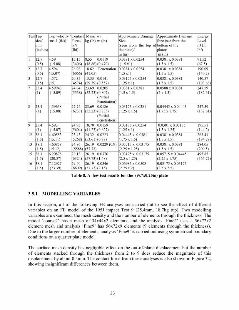
Composite plates of 0.2286x0.1778x0.00638m (9x7x0.25in) were tested under impact. The o.o.p displacement was measured by double integration of the load/time curves obtained from the load cell. Sixteen tests were carried out to see the effect different tup sizes and tup masses have on the o.o.p displacement, contact force and incurred damage. Four of these tests are compared to FE results using SC8R elements in Abaqus/Explicit using a VUMAT. The laminate has 9 woven plies and is modeled as an orthotropic material.

The impact velocity is practically the same for the four tests examined, a value of 4.6ms-1. The test results are detailed in Table 8. As with the larger plate simulations, the critical energy for failure criterion obtained from the impact tests is applied to the RR-layers and Hashin’s 2d stress based failure criteria is used at the woven plies.

32

Test Tup size/ mm (inches)

Tup velocity / ms-1 (ft/s)

Contact Force/ kN (lbf)

Mass/ kg (lb)

δ / m (in)

Approximate Damage Size (seen from the top of the plate)/ m (in)

Approximate Damage Size (see from the bottom of the plate)/ m (in)

Energy Level / J (ft lbf)

1 12.7 (0.5)

4.59 (15.08)

15.15 (3406)

8.55 (18.86)

0.0119 (0.470)

0.0381 x 0.0254 (1.5 x1)

0.0381 x 0.0381 (1.5 x 1.5)

91.52 (67.5)

2 12.7 (0.5)

4.594 (15.07)

26.98 (6066)

18.62 (41.05)

Penetration 0.0381 x 0.0254 (1.5 x1)

0.0381 x 0.0381 (1.5 x 1.5)

190.09 (140.2)

3 12.7 (0.5)

4.572 (15)

20.35 (4574)

13.33 (29.39)

0.0141 (0.557)

0.03175 x 0.0254 (1.25 x 1)

0.0381 x 0.0381 (1.5 x 1.5)

140.57 (103.68)

7 25.4 (1)

4.59943 (15.09)

24.64 (5538)

23.69 (52.23)

0.0205 (0.807) (Partial Penetration)

0.0381 x 0.0381 (1.5 x 1.5)

0.0508 x 0.0381 (2 x 1.5)

247.59 (182.61)

8 25.4 (1)

4.59638 (15.08)

27.74 (6237)

23.69 (52.23)

0.0186 (0.733) (Partial Penetration)

0.03175 x 0.0381 (1.25 x 1.5)

0.04445 x 0.04445 (1.75 x 1.75)

247.59 (182.61)

9 25.4 (1)

4.593 (15.07)

24.93 (5604)

18.70 (41.23)

0.0159 (0.627)

0.03175 x 0.0254 (1.25 x 1)

0.0381 x 0.03175 (1.5 x 1.25)

195.51 (144.2)

12 38.1 (1.5)

4.60553 (15.11)

23.43 (5268)

24.32 (53.61)

0.0223 (0.88)

0.04445 x 0.0381 (1.75 x 1.5)

0.0381 x 0.0381 (1.5 x 1.5)

263.41 (194.28)

13 38.1 (1.5)

4.60858 (15.12)

24.86 (5588)

26.19 (57.73)

0.0229 (0.9) 0.05715 x 0.03175 (2.25 x 1.25)

0.0381 x 0.0381 (1.5 x 1.5)

284.05 (209.5)

15 38.1 (1.5)

6.20878 (20.37)

28.13 (6324)

26.19 (57.73)

0.0376 (1.48)

0.03175 x 0.03175 (2.5 x 1.25)

0.05715 x 0.04445 (2.25 x 1.75)

495.85 (365.72)

16 38.1 (1.5)

7.12927 (23.39)

29.40 (6609)

26.19 (57.73)

0.0546 (2.15)

0.06985 x 0.0508 (2.75 x 2)

0.03175 x 0.03175 (2.5 x 2.5)

Table 8. A few test results for the (9x7x0.25in) plate

3.5.1. MODELLING VARIABLES

In this section, all of the following FE analyses are carried out to see the effect of different variables on an FE model of the 195J impact Test 9 (25.4mm, 18.7kg tup). Two modelling variables are examined: the mesh density and the number of elements through the thickness. The model ‘coarse2’ has a mesh of 34x44x2 elements; and the analysis ‘Fine2’ uses a 56x72x2 element mesh and analysis ‘Fine9’ has 56x72x9 elements (9 elements through the thickness). Due to the larger number of elements, analysis ‘Fine9’ is carried out using symmetrical boundary conditions on a quarter plate model.

The surface mesh density has negligible effect on the out-of-plane displacement but the number of elements stacked through the thickness from 2 to 9 does reduce the magnitude of this displacement by about 0.5mm. The contact force from these analyses is also shown in Figure 32, showing insignificant differences between them.

33

Figure 32 Contact force versus time – Test 9 and FE simulations of test 9.

The average section normal transverse stress, SSAVG6, can be outputted across the plate for any of the elements. SSAVG6 is largely affected by the mesh density, particularly by the number of elements through the thickness. The variation of SSAVG6 is examined at a location that is a distance of approximately 16mm from the centre of the plate along the length. This location is chosen as it is close to the impact site yet it is not affected by some of the irregularities experience at the contact area between the tup and the plate. Every woven ply and RR-layer has three section points but the SSAVG6 is outputted at the single integration point at the centre of each element.

Increasing the number of elements through the thickness provides a sharper stress output, as each stress is calculated from the strains at the element centre: the more elements the less deviation of the average values from the maximum or minimum across the section. Figure 33 demonstrates how larger and more detailed normal transverse stresses are averaged with 9 elements through the thickness compared to 2 elements through the thickness. The ‘B’ in the legend script refers to the element at the bottom of the plate and ‘T’ the element at the top of the plate. With analysis fine9 there are 7 elements also in between. All analyses show that the tensile normal transverse stresses occur on the underside of the plate and the compressive stresses develop on the top side of the plate. The model with 9 through-thickness elements estimates that the positive tensile stresses are larger than the negative compressive stresses, whereas the same model with only 2 through-thickness elements estimates the reverse, although this difference is small. Moreover, the stresses provided by analysis fine9 are of an order of magnitude of up to 50 times larger than those from fine2.

34

Figure 33. The average normal transverse stress versus time, SSAVG6 for FE analyses modelling damage.

The element with the maximum tensile normal transverse stress value for analysis fine9 is at the bottom of the plate where delamination is very pronounced in both the FE simulations and the tests. The high tensile stresses act to pull the plies apart significantly and can cause ‘spawling’.

Based on the tensile and compressive through-thickness test data, the analysis with 9 through-thickness elements is probably a better approximation of the SSAVG6. We know from experiment that delamination in and around the impact site occurred throughout the plate thickness more so near the lower surface. The largest delaminated area visually inspected from the lower surface in test9 was measured as 0.0381x0.03175mm (1.5 x 1.25in) and the cross-section photo (similar to that shown for test 13 in Figure 39) shows prominent delamination of the bottom layer. Thus delamination also occurred at location A on this bottom face and would have been initiated by transverse matrix cracks in the adjacent ply resulting from the large bending stresses and developed largely due to the high normal tensile stresses. The maximum SSAVG6 value obtained from analysis fine9 is 350(106)N/m2, which exceeds the 21 to 40kN quasi-static through-thickness tensile strength values and most likely that also any dynamic values measured in future tests. Thus these predicted tensile SSAVG6 stand-alone values would indicate almost certain delamination at this location.

In test9 delamination is also seen at the top face however the maximum compressive SSAVG6 values predicted in fine9 are of about 75(106)N/m2 which is less than the compressive strength values from quasi-static test data (giving values of over 500(106)Nm2). They are also up to 4

2times smaller than the 400(106)N/m strength values obtained from the 100s-1 strain rate compressive tests on the Corvette composite hull material. These delaminations are therefore largely propagated by the transverse shear stresses. Matrix crushing of the top surface is evident at the centre of the whitened area.

35

The energy criteria used for delamination does not differentiate between compressive and tensile stresses and the through-thickness stresses are not considered where shell elements are concerned. However, the in-plane stress predictions used in the energy equation are affected by the number of elements through the thickness. Figure 35 shows the delamination through the thickness for the quarter plate model FE analysis fine9.

The delamination for analyses fine2 and fine9 is shown in Figure 34 and Figure 35. For both analyses the area of delamination is shown to be greatest for the RR-layer at the bottom of the plate. Analysis fine2 predicts delamination throughout the thickness, unlike fine9 showing damage on the top and bottom surfaces and two intact layers in the centre. Although the tests show delamination more extensively towards the top and particularly at towards the bottom of the plate, there is as yet no C-Scan data to assess the variation in the delamination seen in the FE results. What is known is that the maximum test delamination area at the bottom of the plate is more closely approximate by fine2 than fine9, whereas the opposite can be said about the maximum delamination within the top half of the plate. The number of elements through-the-thickness will affect the position of the 8 RR-layers within the shell elements, thus outputting comparably varying in-plane stresses at the RR-layer integration points. Because the delamination model is one based on plane-stress, the amount of predicted delamination thus varies between models of varying through-thickness mesh densities. Table 9 shows a summary of test 9 results and the FE simulations of this test. In terms of the in-plane critical energy criterion used at the RR-layers, increasing the number of SC8R elements through the thickness does not increase the accuracy of the delamination damage predictions at these layers.

Figure 34. Delamination damage through the Figure 35. Delamination damage through the thickness for FE analysis ‘fine2’. thickness for FE analysis ‘fine9’

The in-plane density of the mesh has no significant effect on the delamination predictions through the thickness and the same delamination area is predicted at the bottom of the plate for coarse2 and fine2 analyses, see Figure 36(a) & (b). However, the maximum through-thickness stresses are noticeably affected, as seen with ‘fine2’ and ‘coarse2’ in Figure 33. The delamination damage for the three different mesh analyses is shown for the RR-layer at the bottom face of the plate for test9 with Figure 36 (a) to (c).

36

(a) coarse2 (b) fine2 (c) fine9. Quarter-plate model

(d) Test 9, bottom face. (e) Test 9, top face.

NOTE: FE analyses of test9, (12.7mm , 17.44kg tup )

Figure 36. (a) to (c). FE analyses, showing delamination damage after impact at the bottom face of the plate, (d) test 9 results for the bottom face, (e) test 9 results for the top face.

Analysis Max o.o.p disp. / m

Max. normal contact force / N

Max. SSAVG6 (ten. & com.)/ 106 N/m2 *

Delam. on bot. RR-layer / 10-3 m2

Coarse2 17.2 30.2 +19 1.11 - 94

Fine2 17.3 28.2 6 -15

1.11

Fine9 16.68 29.9 350 -75

2.41

Test 15.3 26 - 1.45 *Maximum always on centre element, lower face.disp. = displacement; ten.=tension; com.=compression; delam.=delamination

Table 9. Summary of test 9 results and FE simulations of test 9.

Test results of delamination damage at the top and bottom faces of the plates for tests 1, 3, 9 and 13 are shown in Table 10 together with their FE simulations carried out using ‘fine2’ mesh. Maximum delamination damage is captured relatively well, although slightly under-predicted again at the top of the plate. Matrix and fibre damage on the other hand is substantially over-predicted in the FE analyses, with top layers appearing to suffer corner damage also, propagating towards the centre at the top ply. Generally we can say that Hashin’s 2D failure criterion does not work satisfactorily in these simulations, producing unpredictable results.

37

Test Test, delamination area / m (in)

FE, delamination Area / m (in)

FE, matrix damage area/ m (in)

FE, fibre damage area / m (in)

1 BOT: 0.0381x 0.0381 (1.5 x 1.5) TOP: 0.0381 x 0.0254 (1.5 x1)

0.0286 x 0.032 (1.125 x 1.245) TOP: zero

BOT: 0.04445 x 0.060325 (1.7499 x 2.375)

BOT: 0.05715 x 0.03175 (2.25 x 1.25)

3 BOT: 0.0381 x 0.0381 (1.5 x 1.5) TOP: 0.03175 x 0.0254 (1.25 x 1)

BOT: 0.03175 x 0.03175 (1.25 x 1.25) TOP: 0.0127 x 0.0127 (0.5 x 0.5)

BOT: 0.057 x 0.073 (2.24 x 2.87) TOP: 0.035 x 0.058 (1.38 x 2) NOTE: Not included is damage at corners.

BOT: 0.057 x 0.0381 (2.24 x 1.5) TOP: : 0.0381 x 0.016 ( 1.5 x 0.63)

9 BOT: 0.0381x 0.03175 (1.5 x 1.25) TOP: 0.03175 x 0.0254 (1.25 x 1)

BOT: 0.03175 x 0.04445 (1.249 x 1.748) TOP: 0.0127 x 0.0159 (0.5 x 0.63)

BOT: 0.0635 x 0.0889 (2.5 x 3.5) TOP: large cross shape from corners.

BOT: 0.07 x 0.057 (2.76 x 2.24) TOP: 0.0381 x 0.019 (1.5 x 0.75)

13 BOT: 0.0381x 0.0381 (1.5 x 1.5) TOP: 0.05715 x 0.03175 (2.25 x 1.25)

BOT: 0.04445x0.04445 (1.75 x1.75) TOP: 0.015875 x 0.01905 (0.625 x 0.75)

BOT: 0.083 x 0.095 (3.27 x 3.74) TOP: large cross shape from corners.

BOT: 0.073 x 0.07 (2.87 x 2.75) TOP: 0.0381 x 0.019 (1.5 x 0.75)

Top=top layer of plate; bot=bottom layer of plate

Table 10. Delamination results for tests 1,3,9 and 13 and damage prediction from their respective FE simulations.

Even for larger mass differences, simply increasing the mass of the tup will not generally increase the delamination area, as shown with tests1 and 2. Test 2 used a tup mass that was double that of test1. The delamination areas were the same but the extra impact energy in test 2 was expended in penetrating the plate. This was also proven for test 13 and test 12 . In order to increase the delamination damage to the plates and prevent penetration, both the diameter and mass of the tup should be increased in the same test, as demonstrated through tests 15 and 16.

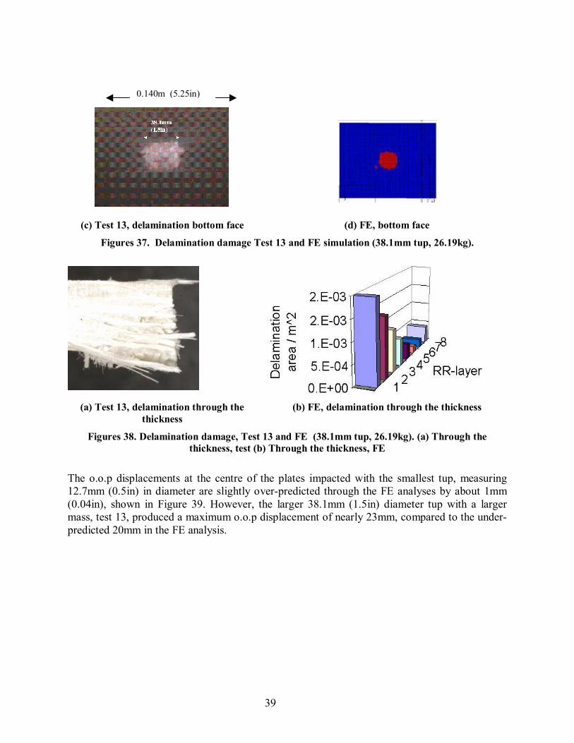
Delamination on the top and bottom face is shown in Figures 37 for test 13 and its FE simulation, and the delamination through the thickness is well captured in the FE model as shown with Figures 38.

(a) Test 13, delamination top face (b) FE, delamination top face

38

( )0.140m 5.25in

(c) Test 13, delamination bottom face (d) FE, bottom face

Figures 37. Delamination damage Test 13 and FE simulation (38.1mm tup, 26.19kg).

(a) Test 13, delamination through the (b) FE, delamination through the thicknessthickness

Figures 38. Delamination damage, Test 13 and FE (38.1mm tup, 26.19kg). (a) Through the thickness, test (b) Through the thickness, FE

The o.o.p displacements at the centre of the plates impacted with the smallest tup, measuring 12.7mm (0.5in) in diameter are slightly over-predicted through the FE analyses by about 1mm (0.04in), shown in Figure 39. However, the larger 38.1mm (1.5in) diameter tup with a larger mass, test 13, produced a maximum o.o.p displacement of nearly 23mm, compared to the under-predicted 20mm in the FE analysis.

39

Figure 39. Out-of-plane displacements at the plate centre versus time for tests 1,3 and 13 and their FE simulations.

Figure 40. Normal contact force versus time for tests 1, 3 and 13 and their FE simulations

The largest difference between measured and predicted contact forces was for test 13; a 37% difference. All the other finite element analyses predict contact forces that are up to 16% higher compared to experiment. However, the maximum contact force for the FE analyses are taken as the peaks of the contact force plots, which do see some pronounced oscillations.

The tup in test 13 did not penetrate the plate but there was substantial damage in the form of delamination and matrix cracking on the bottom of the plate, with fibre failure occurring for some of the fibres in one or two bundles at the plate centre. However, the extent of matrix and fibre damage predicted with Hashin’s criteria is again excessive, see Figures 41 for the lower and higher energy impact tests: test 1 and 13. Had the delaminated layers been physically modeled as separating, the FE o.o.p displacement would be larger and the contact force smaller. Also the transverse stiffness of the plate remains intact through-out the analysis and the transverse strength is likely to have been more affected with the 38.1mm tup than with the 25.4mm tup. This may be one reason why this test saw a proportionally larger over-prediction of the contact force and under-prediction of the o.o.p displacement compared to the smaller tup tests.

40

bot mid top bot mid top (a) Test1 (b) Test13

Figures 41. Matrix cracking on the bottom, middle and top layers of test1 and test13 FE simulations.

The cross-section of the plate in test3 after impact testing, corroborates the large effect of the tensile normal transverse stresses. The plate shows significant delamination near the bottom face of the plate where the tensile transverse normal stresses are acting to pull the plies apart. The top of the plate saw matrix crushing and some surface indentation, a characteristic witnessed in all the impact tests.

Figure 42. Cross-section of the plate in test 6 (12.7mm, 16kg ), showing delamination on the back face.

3.5.2. A VISCOPLASTIC MODEL AT THE RESIN-RICH LAYERS

The out-of-plane displacements obtained from the FE analyses on the small plates are all very conservative and this may be improved with a strain rate model.

For strain-rate sensitive materials, plotting the effective stress and plastic strain produces a discrete curve for different applied strain rates. The following visco-plastic model uses a function developed by Sun (21) that collapses a range of these strain rate plots onto once curve and that was developed around experimental data.

An expression for the plastic strains is required that is both a function of stress and strain rate. Equation (13) is Sun’s power-law relationship between the effective stress and the effective plastic strains for a particular applied strain rate. Here, the parameter ‘B’ is a function of the plastic strain rate.

41

mp a p aε&ε = Bσij = Q ( ) σ (13)

In view of the fact that polymers are sensitive to the hydrostatic stress component (22), the plastic potential function will be a function of the actual stresses. The plastic potential function will be based on the Drucker-Prager yield criterion, as shown with Equation (14), where alpha, α , is a state variable which controls the extent of the effect of the hydrostatic stresses, and the second invariant of the stress tensor.

2f = 1 S Sij + ασ kk )2 − τ 0 = 02 ij (

(14)f = 1 S Sij + ασ kk = 02 ij

An expression for the plastic strain rates can be obtained, as shown in Equation (15), written in terms of the direct stresses and shear stresses respectively. The viscoplastic modulus can be derived as shown in Equation (16).

p ∂f& &ε = λ

∂σij (15)ij

p 1H = ε& p

m σa 1 (16)−aQ ( )

The effect of modelling the resin rich layers as viscoplastic has a significant effect on the out-of-plane displacement results, shown with Figure 43(a) but a negligible effect on the contact force, see Figure 43(b).

(a)

42

(b)

Figure 43. (a)Maximum o.o.p displacement and (b) contact force; comparing Test 9 with FE analysis using mesh 56x72x2; ‘_dam’ models damage and ‘_dam_vis’ models damage and in-plane

strain rate sensitivity.

3.6. CONCLUSION

This work is aimed at modelling the shock loading response of large and small composite panels. The main discussion lies in the implementation of delamination model using resin-rich layers (RR-layers) that are modeled in between every ply.

The simple energy criterion at the RR-layers provides better results over the two simple stress criteria also tested. Here the energy value for failure requires the knowledge of the contact force; an empirical derivation chosen to minimize the errors in the assessment of the resin-rich layer and energy concept. The method for obtaining an expression for this energy that is independent of each test is outside the scope of this work. What we can surmise is that the critical fracture energy value obtained from full scale impact tests was relatively successful in this model unlike the value obtained from mode I fracture tests.

Shell elements were used in the analyses and the energy criterion was thus limited to 2d, excluding the significant transverse shear influence on delamination. The delamination predictions obtained from all the impact test simulations are encouraging but ideally a 3d energy criterion is required. However, the main advantage of this 2d energy criterion for delamination is that it can be applied to shell elements and still obtain a reasonable prediction of the maximum delamination size. The criterion is also simple and quick to use and for the meshes tested is little affected by in-plane mesh density.

The fibre and matrix damage predictions are not so agreeable. Hashin’s 2d stress criteria in the prediction of these two damage modes is not reasonable or consistent between tests. The matrix damage for the large plates (which have clamped boundary conditions), is possibly a little under

43

predicted yet the fibre damage does not occur as extensively as predicted. The smaller, simply supported plate simulations show overly large areas of both damage modes.

The ability to model the rate dependency of the material in the transverse direction could make a substantial difference to the FE results with regard to the out-of-plane stresses and strains. Using layered 3D solid (brick) elements could be one potential solution, however unlike Abaqus/Standard in Abaqus/Explicit the facility for layering currently does not exist.

The maximum out-of-plane displacements predicted in the analyses are quite conservative and can be reduced with a viscoplastic model at the resin-rich layers with a negligible effect to the contact force.

There are restrictions in Abaqus/Explicit that prevent the efficiency of damage modelling of plate structures. The continuum shell elements are new to Abaqus; they can be stacked and appear to provide good normal transverse force predictions. However, the transverse force and stress estimates can be outputted but cannot be used in any subroutine, thus limiting the practicality of the SC8R element and preventing the implementation of a 3D failure criterion. In addition, only the in-plane material properties can be degraded as there is no control over the through-thickness moduli. Although the continuum shells have their advantages over thick shell elements they have yet to be further developed and they are currently of limited practicality in failure modelling.

44

4. IMPACT MODELLING – USING A 3D DAMAGE MODEL WITH COHESIVE LAYERS

4.1. INTRODUCTION

The initiation of damage in composite materials is the point at which the stresses or strains in the material are large enough to incur some permanent deformation in the form of matrix cracking. Stress or strain based criteria have been the most common tools to model failure on a macro-scale but in a basic way, degrading the properties once only down to a residual value. Currently however, continuum damage mechanics (CDM) is becoming increasingly popular and has yet to be introduced in many finite element packages for composite modelling.

Continuum damage mechanics is used to predict the behaviour of a material which has suffered damage initiation as a result of an initial state of stress state followed by damage propagation with increase in stress. Damage accumulation causes changes in the material stiffness which is one of the major contributions to material non-linearity in composites. With reference to damage of composites, Ladeveze (23, 24) and Chaboche (25) produced some of the earlier works in this area. The main limitations of a CDM models however, arise from the testing procedures and suitable experimental data is often difficult to generate.

A variety of constitutive models have been proposed for woven composites. Of particular interest in the field of CDM and impact modelling of woven composites is Iannucci’s and Dechaene’s work. Iannucci et al (26) modelled damage propagation of woven CFRP subjected to impact using shell elements. This was extended for solid elements in work by Dechaene et al (27) and results were compared with composite beam and plate impact experiments. The model was later further validated and a parametric study was carried out by Iannucci (28). Other CDM work includes that by Matzenmiller et al (29), Kollegal et al (30), Talreja’s (31).

Delamination models include the implementation of stress-based criteria at the ply, strain and stress based criteria at resin-rich layers (4, 5), and cohesive layers. Although resin-rich layers can give reasonable results they do not model the physical separation and ensuing contact condition of the delaminated layers. It is evident that to effectively model delamination and thus the reduction in contact force, cohesive elements are an attractive option. Cohesive elements are used by authors such as Espinosa (6) , Chen (7), Scheider (8), Camanho (9), and Turon (10). More recently and more specific to naval composites, Lemmen et al (11) proposed a damage mechanics based model for quasi-static loading of a T-joint panel using a coupled mode I and II linear traction-separation cohesive zone model for delamination and used a damage initiation criterion based on Hashin’s work (12). The model was tested for the quasi-static loading of a T-joint panel and compared with experiment.

Work on dynamic loading of composite plates includes that by Zhou and Greaves (3) who carried out low velocity impact tests on thick GFRP laminates, producing high incident kinetic energy with the use of large masses, plotting the ratio of two impact force thresholds (delamination and final rupture) against delamination area as a way of analyzing the state of damage. Other work includes that by Sierakowski (32) and Davies et al (33), Sutherland et al (34).

45

In this study, small scale and large-scale woven E-glass/vinyl-ester composite plates are tested under impact loading and compared to finite element models in Abaqus/Explicit. The composite evaluated in this study was fabricated at the Naval Surface Warfare Center (NSWC), Carderock Division using a proprietary 24 ounce woven roving E-glass/ Derakane 8084 vinyl-ester.

A user-defined subroutine called a VUMAT is used to write the constitutive behaviour for a nonlinear elastic damaging material model. Modelling the transverse behaviour of thick woven composite plates is important (35), and the plates are thus discretized with solid elements thereby allowing the required 3d degradation of the material via a simple damage mechanics approach. Delamination between plies or groups of plies is also modeled using cohesive elements and a traction-separation law available in Abaqus/Explicit. Cyclic tests were carried out to obtain damage parameters and the FE models are validated against large-scale impact tests on GFRP panels. The material model serves to provide a relatively simple but effective, conservative method of modelling damage and material behavior without being wholly reliable on complex testing procedures.

4.2. THE DAMAGE MODEL

The damage model can be divided into three parts: damage initiation, matrix damage only and combined matrix and fibre damage propagation until full failure. In the present study, three separate functions are tested to predict global damage initiation, amongst them Hashin’s 3d failure criterion and one minor variations of this criterion are tested. Two transverse maximum stress criteria are also tested to separately predict the initiation of transverse damage at the woven plies.

The propagation of in-plane matrix damage and fibre damage is modeled using linear strain criteria. The transverse (through-thickness) damage propagation is treated separately with individual maximum stress criteria. The 3d state of stress related to the laminate is represented with Figure 44.

Figure 44. 3d stresses

There are several assumptions associated with this damage model, some of these highlighted here:

46

i. The term damage is representative of the volume of numerous cracks at a material point. This assumption implies that the crack size must be very small in relation to the volume associated with the material point. ii. In this model, the damage term means the same as stiffness reduction. iii. Keeping with the first and second laws of thermodynamics, the damage is irreversible and

therefore the damage function is monotonically increasing, with the form:

d(t) = max {d(τ)}τ≤ t

Where τ is the previous time and t is the current time, this condition states that the damage in the current time is dependent on the maximum attained damage during the loading history up to the current time. iv. The material is elastic damaging and therefore the strains comprise of elastic strains and

damage strains only. v.Damage growth does not always lead to full failure of a material point or indeed a ply. vi. Damage can only develop once the damage initiation function is activated to allow this.

The shortfall of a non damage mechanics approach is the immediate reduction of material properties when damage is first predicted, rather than the gradual reduction of properties from damage initiation up to full failure. The later method represents the more realistic behaviour of a composite under a damaging load. The rate at which damage occurs is then dependent upon the propagation criteria. Cyclic tests are a useful method of incurring gradual damage in a material to see the effect on the moduli i.e. how the moduli degrade with increase in cyclic loading. Sometimes this is carried out until failure. In the current work, cyclic loading is carried out until significant matrix damage has occurred but no fibre failure. Cyclic loading tests are chosen because with current detection methods, it is impossible to detect the gradual moduli changes occurring to the material under a dynamic load. A cyclic test is therefore a quasi-static alternative to producing damage in a gradual way under a given stress. A hydraulic testing machine is used as with standard tensile and compression test coupons.

4.2.1. DAMAGE INITIATION

Three criteria are tested to initiate global damage, i.e. damage on all planes: Hashin’s 3d criterion, a small modification of this and an equivalent strain criterion. A separate damage initiation criterion for the transverse planes is also evaluated.

Hashin’s 3D criterion (12) for matrix cracking uses two equations; one when the transverse σ22 stress is compressive and the other for when it is tensile. The fact that the failure envelopes were designed for unidirectional laminae is manifested when the criteria are used on an orthotropic laminate, predicting a damage pattern that is always rectangular in shape. In this work this is amended by replacing the orthogonal stress σ22 with an average of both the normal in-plane stresses. The FE analysis results are still not satisfactory with this formulation, since the tensile (bottom) side of the plate is always first to damage and continuing to do so predominantly more than the top of the plate. Hashin’s formulation appears to be inadequate for this problem as

47

damage initiation is predicted very late on in the analyses and is then followed by over-extensive areas of damage initiation.

The effective strain criterion suggested by Williams (2), is shown in Equation (17) which here includes the through-thickness strain component so that it can be used for 3d predictions.

Equivalent strain function, a 3d version of that used by S K Williams.

2

εx εy εy 2

γxy 2

γyz 2

γzx 2

εzz

2

≥ 1 (17)

Fi =

ε K

x

−

K

L +

L

+ S

+ T

+ U

+ V

Where K, L, S, T and U are the strains to failure of the ply in the in-plane x-direction, the in-plane y-direction, the in-plane shear direction, and the two transverse shear directions yz and zx respectively using standard tensile and compressive tests.

In some analyses, a separate stress criterion for out-of-plane damage initiation is tested and for these Equation (17) is used to only predict in-plane damage, without the normal transverse strain component ε33. The first out-of-plane stress criterion tested is one of simple maximum stress, Equations (18), after which the modulus is simply reduced once only down to its residual value, thus requiring no damage propagation criterion. The second criterion is a quadratic stress function, Equation (19), the same as Brewer and Legace’s delamination criterion. This is chosen because it requires readily available strength data and it is also more conservative than using the single maximum stress criterion. Once this quadratic criterion is met, the modulus is reduced gradually until the individual out-of-plane stresses are equal to their ultimate stress values.

σ33

=≥ 1 , σ23 σ13 ≥ 1, ≥ 1 (18)

ZT S23 S31

2 2 σ33

2 σ23 σ13 + + ≥ 1 (19)

ZT S23 S31

4.2.2. DAMAGE PROPAGATION

A test that produces stable crack growth is required to characterize the effect of damage propagation in composites. Unnotched coupon tensile tests used in the past produce unstable crack growth soon after the start of any damage but cyclic or fatigue loading is one method of getting stable crack growth by developing the damage very slowly. Work by Talreja and other authors show that changes in moduli seen in fatigue testing of coupons can be used to quantify the damage incurred.

Inelastic (permanent) strains are caused by inelastic damage to the material (such as matrix cracking) and plastic strains (from plastic flow of the material). In this macro-scale model it is not possible to separate the two, therefore both strain contributions are referred to collectively as

48

‘inelastic strains’. GFRP plastics are generally strain-rate sensitive, however to reduce the testing complexity that would be involved with coupled strain rate and cyclic testing, (26), the elastic constants are assumed to be independent of the strain rate of the material.

It is important to note that there is no coupling between the in-plane stresses with the transverse stresses, therefore each propagation criterion is unconnected.

4.2.2.1. IN-PLANE DAMAGE

In this work all the elastic moduli are individually linearly degraded to 10% of their original value in two gradual steps and can only occur once damage initiation is activated. In this model pure matrix damage occurs first followed by combined matrix and fibre damage until full failure. The damage is dependent upon a scalar potential function F, which is a summation of the damage initiation function, the matrix failure function Fm and the fibre failure function, Ff, see Equation (20) and Figure 45. Full material point failure occurs when Equation (21) is met, where FII is the function at the start of fibre failure and FIII is at full failure. The functions for matrix and fibre failure are both simple strain functions that define the development of damage.

F = Fi + Fm + Ff Total scalar potential: (20)

F = FI + FII + FIII = 3 Scalar potential for full failure (21)

The in-plane damage variables are denoted by d1, d2, ds. The damage criteria are applied individually to each of the orthogonal in-plane directions 11 and 22 using the damage variables d1 and d2 respectively. The final damage function d, expressed for each of the in-plane directions is shown with Equations (22) and (23). The damage coupling criterion for the in-plane shear damage variable ds was proposed by Williams (2). The matrix damage parameter is in the range of dI < < dII , and the damage potential for matrix failure Fm is in the range of FI < < F , see d Fm II

Figure 45.

d1 = d1m + d1f (22)d2 = d2m + d2f

d2 2d = + − d d s x dy x y (23)

The term ‘damage’ is generally referred to as the proportion of damaged material and although a material cross-section may be 80% saturated with cracks, the loss in stiffness may not be necessarily equal to 80% of the original stiffness. Ideally, in order to have two variables: one representing the damaged area and another representing the reduction in stiffness up to failure requires the extraction of the matrix damage saturation value dsat. This parameter was not obtained for the current material model therefore the percentage of stiffness loss is here equal to the percentage of ‘damage’. The damage variable attributed to the matrix cracking only is obtained from cyclic tests and is equal to the ratio of the damaged modulus divided by the

49

0

original intact modulus. For most of the models the strain thresholds used in the damage potential strain functions are obtained from tensile cyclic tests and the effect of differentiation between compressive and tensile stresses is only tested in one model.

The original intact moduli, Eij , are degraded as shown with Equations (24). A schematic showing an in-plane damage variable with modulus degradation is shown in Figure 46.

Eij = Eij (1 − dij ) (no summation in ij) (24)

dIII

dII

FII F =1

d

F

Fm Ff

dm

df

0

dsat

=0.9

=0.1

=1 III

matrix only damage

= unknown

Figure 45. Damage parameter d as a function of F.

E

E0

Em

E=10%E0

Damage from matrix failure

Damage from matrix and fibre failure

dI dII dIII d

Figure 46. Modulus reduction as a function of d, for a given in-plane direction.

50

4.2.2.1.1. Matrix damage development

Here we test two scalar potential functions for matrix cracking, Fm. The first is given by a linear strain function Equation (25); where ε0 is the strain at which matrix damage initiates, ε is the actual instantaneous strain calculated in the analysis and εf is the strain at which fibre damage initiates. The other is a dissipated energy function, Equation (26). The energy absorbed by the material per unit volume is a function of the materials’ elastic properties and the stresses in the material. Once damage has initiated, the material degrades and the elastic properties of the virgin material diminish which must be accounted for in the constitutive equations. The mean value of the energy density for a damaged material, represented with Equation (27) for 2d energy, will therefore be different to that for an intact material.

(ε ε − ε0 ) (25)fF = m (ε ε − ε0 )f

σ̂ − ϒ0 (26)

F = 2E m ϒ − ϒ0max

2 2 2 2 − σ12

2 (27)1 σ11 σ11 σ22 σ22− −+ − − 2 ν12 σ σ + +d E

Φ = 1

11 22 2 E (1 − d1) E1 E (1 − d2 ) E2 G12 (1 − d3) 1 2

The formulation of Equation (25) suggests that damage cannot initiate until ε0 has been reached. However, this can be potentially over-ridden by the damage initiation function. It is found, that the damage initiation function flags the start of damage at a strain that is larger than ε0 and therefore over-rides this strain value.

4.2.2.1.2. Cyclic test data

Cyclic tests were carried out to obtain an approximation of the matrix damage initiation strain and the fibre damage initiation strain.

Cyclic tests were performed on twelve WR E-glass/ Derakane 8084 vinyl-ester coupon coupons by the USNA. Three tests were performed in the fill direction and three in the weft direction; both in tension (coupons Warp-T1,T2, T3 and Weft-T1,T2,T3) and in compression (coupons Warp-T3,T4,T5 and Weft-T3,T4-T5). The cyclic loading program for tension and compression was exactly the same other than the direction of strain. The loading frequency was carried out at 0.5Hz in triangular waveform under strain control. The strain was applied from 0% to 0.5% (5E3 strain), 0.75%, 1% and 2.5% in increments of 0.25%. Five loading cycles were carried out at every new increment of strain.

The actual termination of the cyclic tests took place before a strain of 2.5% was reached, when audible pops were heard and the mean strain shifted causing a shift in the mean load in the

51

direction of loading. It is difficult to know with certainty the exact point at which fibre cracking initiated however a reasonable approximation was taken as the termination of the cyclic tests, based on this information.

Table 11 provides information on the stress and strain at the last cycle and the final damaged modulus for the twelve coupons tested. The data reveals that a larger amount of damage was suffered by the tensile coupons per unit strain. The tests also show that the warp direction is stronger than the fill direction and generally develops a little less damage at the same loading strains. The FE model in this paper however, does not include this difference in the warp and weft and more simply applies the average material properties obtained for both directions. This includes the value for the percentage of stiffness lost in the cyclic tests. A typical strain versus damage (stiffness reduction) for a compression and tension cyclic test in the fill direction is shown in Figure 47 and Figure 48 respectively. The tests terminated earlier for the coupons tested under compression over those under tension.

Max N0 of cycles

Maximum stress at last cycle /MPa

Maximum strain at last cycle / strain

Initial modulus / GPa

Final damaged modulus / GPa

Maximum damage (stiffness lost)

Tension Warp-T1 38 485.04 0.0248 28.78 23.86 0.17 Warp-T2 40 511.97 0.02245 28.05 22.85 0.19 Warp-T3 36 457.83 0.02024 27.98 23.67 0.15 Fill-T1 36 371.82 0.02158 23.72 18.29 0.23 Fill-T2 31 315.75 0.01853 23.53 17.95 0.24 Fill-T3 36 393.07 0.02237 24.09 18.75 0.22 Compression Warp-T4 21 412.32 -0.01490 28.60 27.99 0.05 Warp-T5 25 382.91 -0.01503 27.69 27.07 0.02 Warp-T6 24 385.20 -0.01502 27.96 27.41 0.02 Fill-T4 32 400.09 -0.01896 24.78 24.10 0.03 Fill-T5 32 356.99 -0.01504 26.08 25.73 0.01 Fill-T6 25 338.9 -0.01508 25.27 24.36 0.04

Table 11. Summary of cyclic test data

The strain/stress plot in Figure 50 shows the non-linear damaging relationship ending at a maximum tensile stress of about 500MPa, noting that the average tensile strength of the composite from standard tests in the orthogonal in-plane direction is 365MPa. The damage property parameters used in Equation (25) are shown in Table 12. The strains are obtained from the strain-damage plots for both fibre directions (‘1’ and ‘2’). The tension and compression damage variables d1 and d2 for these plots are calculated from the degraded moduli from experiment, using Equation (15).

52

Y1

0.08 0.1

0.12 0.14

d1

0

-0.01

0.01

0.02

0.03

-2.0E-02 -1.5E-02 -1.0E-02 -5.0E-03 0.0E+00

d1

0.25

0.2

0.15

0.1

0.05

0 strain 0.E+00 5.E-03 1.E-02 2.E-02 2.E-02 3.E-02

ε0 = 0.005 strain εf = 0.0248

Figure 47. Strain versus damage, compressive Figure 48. Strain versus damage, tensile cycling cycling in the warp direction, coupon T5. in the warp direction, coupon T1.

0.2 600 0.18

500 0.16

Max

str

es /

MPa

400

300

200

d1

0.06 0.04 100 0.02

0 0

0 500 1000 1500 2000 2500 0 0.005 0.01 0.015 0.02 0.025 630 1

Y /Pa 2325 strain

Figure 49. Damage energy release rate versus Figure 50. Stress-strain plot for tension Warp-damage, tensile cycling in the warp direction, T2 coupon.

coupon T1.

Cyclic testing ε0 * εf εmax dII

Tensile 0.005 0.0248 0.04 (Williams (2)) 0.195 Compressive -0.005 -0.015 0.04 0.018

* Over-ridden by damage initiation function.

Table 12. Damage propagation parameters.

4.2.2.1.3. Fibre damage development

F Fibre damage takes place when the scalar potential function for fibre failure, Ff, lies in the range

II < Ff < FIII and the damage variable is in the region dII < < dIII .d

The potential function is based on the strain to failure of the fibre, εmax, as shown with Equation (28).

53

Ff ε11 (28)=

εmax

The strain at rupture, parameter εmax, is not easy to estimate analytically and requires test data. As one would expect, the strain to failure of the undamaged composite material is found to be lower than that of the damaged material in the softening zone, as discussed by Williams (2) with reference to Kongshavn and Poursartip’s work on CFRP. This work involved growing damage in a stable manner using a compact tension specimen then carrying out tensile tests to failure using material from the damaged portion of the specimen, demonstrating rupture strains of 3-4%. Tensile tests to failure for the undamaged material on the other hand, gave rupture strains of about 1.5%. Williams et al used a strain to rupture value of 0.04 in their model. Thus, due to lack of experimental data for fibre failure for the woven E-glass/vinyl ester in the present work, we use the strain value of 0.04 to depict full fibre failure and therefore full material failure. In reality however, this strain may be larger for this woven roving.

4.2.2.2. TRANSVERSE DAMAGE

4.2.2.2.1. Transverse damage of the woven plies

Although transverse shear matrix cracks within the plies will act to reduce the transverse properties, delamination and ply-shear out are two of the principal damage mechanisms (3) and here delamination is separately modeled using a cohesive zone model (see section 4.2.2.2.2). With thicker plates not every ply in the FE model can be analysed for delamination thus transverse damage modelling at the solid layers is important in addition to delamination modelling. Unless specified, damage initiation is defined with either the global equivalent strain criterion, Equation (21), or a separate stress criterion; Equations (18) or (19). The moduli of the solid elements are gradually reduced to 10% of their original value using a maximum stress criterion, Equation (29), unless Equation (18) is used for damage initiation. The difference between the compressive and tensile behaviour of the material is incorporated using the relevant ultimate stress values from standard transverse compressive and tensile tests.

(29)dij = 0.9 σ

σ

ij

ij , where i,j=2,3. No summation in ij. max

4.2.2.2.2. Delamination damage

A cohesive zone model is used to model delamination between the woven plies. Out of the various cohesive zone models available in Abaqus (20), a traction-separation response is chosen for all the analyses. Here, a mixed mode damage initiation criterion is applied which means that the loading in the transverse normal and shear directions (mode I and modes II & III respectively), are coupled. This implies that damage will most likely initiate at a stress that is smaller than the maximum stress for failure for the individual mode.

54

0

0

The maximum attained value during the loading history of equivalent mixed mode displacement, u , is used to detect the damage at the interface. The initiation of delaminationm

damage is determined when a maximum nominal stress criterion, as shown in Equation (30), is maxequal to one. This occurs at mixed mode stress values of τi = τi , where i=n,s,t, represents

each of the three modes of delamination and the Macaulay brackets are an indication of positive maxstresses only (i.e. only relevant to the normal stress τ ). Τi in the equation, also shown inn

Figure 51, is the maximum stress for the pure modes (i.e. when no other mode is acting).

2 2 2 (30)

maxτ

max maxτ τn

t 1s+ + =

max max maxΤn Τs Τt

The quadratic stress criterion can also be written in terms of the displacements, Equation (31) by substituting the maximum stresses with the product of the penalty stiffness and the initiation strain.

2 2 2

(31)0 0

u u un

t =1s+ + U n

0 0

U U ts

It is assumed that the mode I stress does not contribute towards delamination damage when this stress is compressive and therefore under this loading mode I behavior is excluded from the equation.

initiation criterion

ut f

um fUt

f

ut 0 un

0

um 0

un f

Un f

Τn maxΤt

max

τt max

τm max

τn max

Ut 0

Un 0

stress

shear displacement

normal

1 2

max

max 2

max

max 2

max

max

= Τ

+ Τ

+ Τ t

t

s

s

n

n τττ

displacement

Figure 51. Mixed-mode traction-separation

55

The delamination damage evolution criterion used here is one based on fracture energy, shown by Equation (32). The softening behavior can be either linear or exponential in Abaqus and for validation of a simpler model, a linear case was chosen. The power indice defines the shape of the failure locus and is typically equal to one or two. There is still discrepancy as to which power indice should be used or if indeed the power law criterion is adequate for certain composites or not. Opinions are varied as highlighted with work by Goyal et al (36) and Camanho et al (27, 27). However, according to Camanho there is no reliable mixed mode loading criteria for delamination propagation that involves mode III because of the lack of adequate mixed-mode tests that includes mode III activity.

G α

α

n sf (G) = + Gt

α

+ G

, α = 2 (32) GnC GtC GsC

The length of the cohesive zone is important in order to select an appropriate mesh size. The length of the cohesive zone is defined as the distance from the crack tip to the point where the maximum cohesive traction is reached. All the expressions to estimate the length of this cohesive zone, Lc, have the same form, and only differ in a multiple factor n, see Equation (33), where σmax is the maximum interfacial strength. Hilleborg proposed the relationship shown in Equation (33) with n equal to 1.

L = nEGc (33)

c σ2 max

In an FE analysis, the cohesive zone must be discretized with a certain number of elements. The element length can be simply defined as shown in Equation (34), where N is the number of elements. The exact number of elements required is still being debated. Some researchers have proposed more than 10 elements, others 2 to 5 (10), whereas Camanho and Davila (37) believe 3 elements is adequate enough, based on a parametric study on a DCB specimen.

Lc (34)L = e N

56

4.3. RESULTS AND DISCUSSION

4.3.1. SMALL PLATES (0.2286X0.1778X0.00638M)

Although a number of impact tests were carried out using different tup masses and tup sizes are detailed, only a few of these tests are discussed here, see Table 13. Some of these tests were earlier modeled with the resin-rich layer model and are detailed in Table 8 and Table 10.

The tests in Table 13 are in order of impact energy: ‘A’ referring to minimum (180J) and ‘H’ maximum (284J). A summary of the FE predictions in terms of peak contact force, maximum out-of-plane displacement and damage area presented in the following sections, are shown in italics, inside square brackets. Some of the tests were repeated and only the repeat of test F(7), ‘testF(8)’, is presented because it gave dissimilar results.

Unless otherwise specified, all except two of the analyses use the 3d equivalent strain criterion for damage initiation, Equation (17), and the linear strain criterion for matrix damage propagation, Equation (25) and model through-thickness damage at the woven plies. A model exclusive of through-thickness damage at the woven plies is labeled as ‘2d’. The variation in the normal transverse modulus obtained from standard tensile tests is significant, with values ranging from 6.98 to 22.68kN/mm2, and the average value is used in the subsequent analyses. Unless otherwise specified, the mesh used in the analyses is a relatively coarse one; ‘P1T1’, see Table 14. The plates are made-up of nine woven plies and the FE analyses model either 8 or 4 cohesive layers, as indicated.

57

Test Tup size/ mm

(inches)

Tup velocity / ms-1 (ft/s)

Mass/ kg (lb)

Contact Force in kN (lbf)

δ in m (in)

Approximate Damage

Size (Top) in m (in)

Approximate Damage

Size (Bottom) in m (in)

Energy Level

in J (ft lbf)

[FE in kN] [FE in m] [FE in m]( cohesive layer ‘c’)*

[FE in m] (cohesive layer ‘c’)*

[FE in J]

1805) A (20

(1) 25.4 (14.96)

(38.36) 17.47 25.72 (5783) 0.01532 (0.603)

(133.31) 180.74

[26.9] [181.6] B(9) 25.4

(1) 4.593 (15.07)

18.70 (41.23)

24.9 (5604) 0.0159 (0.627) 0.03175 x 0.0254 (1.25 x 1)

0.0381 x 0.03175 (1.5 x 1.25)

195.51 (144.2)

C(21) 25.4 [26.4] [0.0184] [0.044x0.044] (c5) [0.038x0.038] (c3) [197.8]

197.80 (1)

(14.96) 19.04 (41.98) 27.16 (6105) 0.01643 (0.635) (145.89)

[28.4] [0.0185] [197.96 ) D(10) 25.4

(1) 4.59638 (15.08)

20.34 (44.84)

27.9 (6263)

0.0165 (0.651) 0.0381 x 0.03175 (1.5 x 1.25)

0.0381 x 0.03175 (1.5 x 1.25)

217.41 (160.35)

E(22) 25.4 (1)

(14.96) 21.99 (48.47) [27.8]

28.2 (6330) [ 0.0192]

0.01732 (0.682) [0.052x0.038] (c7) [0.043x0.033] (c4) [215.2 ]

228.38

(38) [0.01857]

0.0381 x 0.0381 0.0508 x 0.0381 [228.56]

(168.442)

247.59 F(7)(1)

25.4 (15.09)

4.59943 (52.23) 23.69

(5538)24.6

[ 0.0200] 0.0205 (0.807)

(1.5 x 1.5)

[0.0478x0.043] (c7)

0.03175 x 0.0381 (1.25 x 1.5)

(2 x 1.5)

[0.0382x0.033] (c2&4)

0.04445 x 0.04445 (1.75 x 1.75)

(182.61)

[250.64]

247.59 (182.61)

F(8) 25.4 (1)

4.59638 (15.08)

23.69 (52.23)

[27]

27.7 (6237)

(Partial Penetration)

0.0186 (0.733)

G(23) (1)

25.4 (14.96) 25.99 (57.29) 27.8 (6240)

(Partial Penetration)

0.01935 (0.762) (199.09) 269.93

[30] [0.0191] [270.15] H(13) 38.1

(1.5) 4.60858 (15.12)

26.19 (57.73)

24.9 (5588)

0.0229 (0.9) 0.05715 x 0.03175 (2.25 x 1.25)

0.0381 x 0.0381 (1.5 x 1.5)

284.05 (209.5)

[32.37 ] [ 0.0208] [0.044x0.044] (c7) [ 0.044x0.044] (c3) [277.1]

* c1 refers to cohesive layer number one (8 cohesive layers, c1 to c8, numbering starts from the bottom of the plate. Top face is impact face). FE results are shown in italics inside square brackets in metric units only.

Table 13. Test and FE results, in order of increasing impact energy.

Region mesh Average element size in impact zone /mm P1 Plate mesh, 28x36 = 1008 surface elements 3.175 P2 Plate mesh, 1128 surface elements (finer in impact site) 1.6 T1 Tup mesh, 12 elements on dome contact surface 4.68 T2 Tup mesh, 145 surface elements on dome contact surface 1.02

Table 14. Mesh types

58

The test producing the second lowest impact energy is Test B(9). The tup used for test B(9) has a 24.5mm diameter and a mass of 18.7kg, see Table 13.

The significance of including a damage model in the impact analysis is demonstrated with Figure 52. The contact force is about 25% larger for the analysis modelling no damage than for the other two damage models and because it is stiffer, it picks up the higher frequencies. The effect of using the linear strain criterion or energy criterion for matrix damage initiation is very small on the contact force and negligible on the out-of-plane displacement.

The use of cohesive layers not only reduces the peak contact force but also appears to stabilize the shape of the contact force, also demonstrated with Figure 52. A likely reason for this is the extra energy absorption at these layers. Without the cohesive layers, the excess energy that would normally go into delamination would go into more matrix and fibre damage, causing the elements to excessively deform. Inclusion of these cohesive layers not only has the effect of further reducing the stiffness of the plate but further decreases the detection of some of the higher frequency components.

By default, Abaqus/Explicit uses finite sliding for contact pairs and it is the more robust algorithm for this type of analysis. When using hard kinematic contact with the pure master-slave algorithm as in this case, the master surface (in this case the tup) may still penetrate the slave surface even after the acceleration corrections for the master and slave nodes have been made. The mesh influence on the contact computation is not discussed here, however for minimal dependence on the mesh density the analysis should be run as finite sliding as opposed small sliding. Figure 53 shows how there is negligible difference between analyses ‘co8_p2t2’ and the analyses using the coarser tup ‘co8_p2t1’.

Figure 52. The effect of including the cohesive Figure 53. The effect of through-thickness layers, test 9. damage with a full delamination model, test 9

The effect of doubling the damage parameter, dII shows to have negligible effect on the contact force. The reduction in modulus obtained from tensile cyclic tests is 19%, giving dII=0.19. This value is doubled in analysis ‘co4_E33(6.98)_strain(dII0.38)’ but all other parameters including the strain at the start of fibre damage, εf, are kept the same. The rate of damage up to strain εf may not be that significant, although this would have to be properly verified by testing even larger values of dII and for different impact conditions. Moreover, increasing the rate in the early

59

part of the loading curve but keeping all other parameters constant, brings about a decrease in the rate of damage after a strain value of εf, as shown with Figure 54.

FII FIIIFI

d d

dII

dII

F(ε)

dI

III = 1

=0.38

=0.19

Figure 54. The effect of increasing dII. Figure 55. Degradation contours of modulus E11, analysis Co4_ strain, test9.

The strain values from the cyclic tests have been taken from the tensile loaded coupons and used for both compressive and tensile in-plane conditions. Differentiating between compressive and tensile in-plane strains makes a negligible difference to the maximum o.o.p displacement but has the effect of increasing the maximum contact force by a mere 3%.

The damage areas detailed for a few of the tests shown in Table 13 were taken by measuring the largest discoloured areas seen from the top and bottom faces of the plates. These principal damage regions are not necessarily found on the surface of the plate and are presumed to lie within the half of the plate nearest the inspected face. It is reasonable to say that the only damage that can be seen with clarity with the naked eye is delamination damage and/or a heavily cracked region. The extent of matrix cracking has yet to be measured from experiment and could extend further than the delaminated areas.

The extent of predicted delamination at the end of the impact when the tup has rebound back to a position of zero displacement, is shown in Figures 56(a) for test B(9), with experimental photos for the test shown in Figures 56 (c) and (d). We can see from the test figures that the largest delaminated area that can be visually seen from the bottom face may be a few layers above the bottom face. This area is estimated as 0.0381 x 0.03175m compared to 0.035x0.035metres which is the largest delaminated layer within the three bottom layers of the plate according to the simulation. The delaminated top layer in the FE analysis is comparably larger but generally the results are promising.

60

(a) Co4_ strain (b)) Co4_strain_TT2

38mm

32mm

25.mm

32mm

(c) Test 9, bottom face. Note: full extent of plate is (d) Test 9, top face. Note: full extent of plate not available to show. is not available to show.

Figures 56. (a) & (b) Delaminated regions shown in black, at the end of the analysis for test 9, (c) & (d) experimental results

The in-plane damage prediction is shown in Figure 55, for test 9 analysis ‘co4’. The proportions of pure matrix damage and combined matrix and fibre damage can be approximated from these modulus contours using Equations (24). The maximum area of damage appears quite extensive, however the predicted modulus reduction in these wider regions is only small, comprising of matrix cracking only. The model shows that more in-plane damage is seen at the bottom than at the top of the plate. Although this cannot as yet be proven with scanning electron microscope evidence, the largest whitened region appears at the bottom of all the impacted plates and this correlates well with Mouritz’s work (39). Cracking of both the matrix and glass fibres was observed in the tests, which is evident also in the FE simulations.

Exclusion of the through-thickness material degradation at the woven plies for a model with half the number of inter-ply cohesive zones has the effect of increasing the contact force, as shown with ‘co4_2d’ compared to ‘co4’ in Figure 57. Modelling the full number of cohesive layers (i.e. 8) and applying a 2d degradation model at the woven plies appears to make negligible difference to the contact force compared to a 4 cohesive layer model.

The analyses ‘co4_TT2’ and ‘co4_TT1’ use the separate stress criteria for damage initiation through-the-thickness, Equation (18) and (19). These criteria generate negligible transverse

61

damage and the behaviour resembles that of the 2d damage model (‘co4_2d’) at the woven layers, see Figure 57 & Figure 58.

Figure 57. Effect of modelling through-thickness Figure 58. Test 9. Varying transverse damage damage at the woven plies, Test B(9). initiation criteria.

Modelling transverse degradation at the woven plies for a full-cohesive layer model is an area which much be examined further. Transverse stresses will be responsible for delamination but also cracking of the matrix within the ply, particularly for thicker plies. The effect of excluding the transverse degradation at the woven plies for an 8 cohesive layer model is shown in Figure 53 for test B(9), with ‘co8_p2t1_2d’ and ‘co8_p2t1’. Figure 59(a) and (b) with ‘co8_p2t2’ and ‘co8_p2t2_2d’ for the higher energy plate impacts tests F(7)/G(8) and test H(13) respectively. Test H(13) also uses a larger 38mm tup. The effect of full transverse damage modelling (i.e. 8 cohesive layer modelling and transverse degradation at the woven plies) has a significant effect on the contact force in Test H(13). Here, a coarse 4 layer model does not sufficiently reduce the contact force but an 8 cohesive layer model improves on this. However, despite the significant transverse modulus degradation the peak contact force is still a little high for this simulation, indicating other factors of influence such as the loss of flexibility by using solid elements over shells and/or contact concerns.

The increased element instability seen with a full transverse damage model is not only dependent on the through-thickness moduli degradation rules but also on the incident kinetic energy, the tup diameter and mesh density. One must also note that experimentally the plates in tests F(7) & F(8) experienced partial tup penetration. This type of event is not accounted for in the model and thus one prominent reason for the enhanced element deformation in these simulations. For a given tup diameter, clearly the greater the impact energy the larger the damage inflicted, which is represented by a reduction in modulus, and the more liable the instability. Ideally, to reduce the element distortion in the model, the failed elements would need to be deleted. However, this is often not practical or realistic unless the mesh is very fine, if not it may only add to the model’s instability or give erroneous results.

The mesh density is less influential when the through-thickness damage is excluded, as shown with ‘co8_p1t1_2d’ and ‘co8_p2t2_2d’ in Figure 59(b) for test H(13) but very influential in a full 3d damage model as seen with ‘co8_p1t1’ and ‘co8_p2t2’ in Figure 59(c) for test D(10). Despite the instability and early termination of the analysis, compared to the experimental the

62

maximum out-of-plane displacement and contact force predictions for test 10 are only over-predicted by about 10% and 5% respectively, using the ‘co8_p2t2’ model.

(a) (b)

(c) (d)

(e) (f)

Figure 59. Contact force predictions for a) tests F(7)&(8), b) test H(13), c) test D(10),d)tests20 & C(21), (e) test E(22), (f) test23

Good contact force predictions for the lowest and intermediate impact energy tests A(20), C(21) and E(22) are shown in Figure 59(d) and (e). There is also a trend amongst all the analyses that shows an increase in the asymmetry of the contact force-time plots with increase in impact energy, which indicates an increase in damage (34). Significant fibre failure associated with high impact energies is demonstrated with a sudden drop in contact force, which was predominant

63

with test G(23), Figure 59(f). The FE model of this test becomes very unstable at this point of impact, and although it provides a good peak contact force, the unloading part of the curve contains many sporadic peaks that are no reflection of the actual contact behaviour of the panel.

A plot of displacement against contact force for several of the 1 inch tup tests (low to intermediate impact energies), Figure 60, shows some important features during the loading event. The plate width-thickness ratio of these plates is large enough for membrane action to take effect and this is apparent with the increase in the stiffness of the plate from the start to the finish of loading.

Some of the peaks and troughs present in all the experimental plots are replicated in the FE models, here demonstrated for test C(21) and it’s simulation ‘FE_test21’. At peak ‘1’, the FE model predicts no damage, and the reduction in contact force may be attributed to the compression of the top element and the contact definition. Peak ‘2’, coincides with the start of in-plane damage see Figure 61(a), at the bottom of the plate and shear induced delamination which begins at the bottom ply. At peak ‘3’ significant drops in the in-plane modulus takes place for those elements at the centre of the plate, particularly at the bottom of the plate, as shown with Figure 62 (a), (b) and some fibre damage begins, see Figure 62 (a) . From this point onwards more elements in and around the impact site begin to loose stiffness, see Figure 62 (c), where we can see some of the bottom elements with strains of over 0.0248, greater than the strain for start of fibre damage εf (see Table 12), and further significant delamination takes place. At peak ‘4’, full failure occurs and unloading begins. Figure 62 (d) shows how throughout the loading history, the plate elements in the impact site other than those towards the bottom of the plate degrade less in comparison. One obvious difference between the test plot and FE plot includes the lack of un-recoverable (irreversible) energy for the FE version and its rotational shift relative to the test by over-predicted out-of-plane displacements and longer contact times.

Figure 60. Experimental results for some of the 1 inch tup impact tests

64

Figure 61. FE_testA(20) , (a) Start of in-plane damage, (b) start of delamination damage (initiating at the bottom layers)

(b)(a)

(c) (d)

Figure 62. FE analysis results for test C(21). (a) Reduction in the in-plane modulus during the full impact time for a few elements at the bottom centre of the plate shown in (b); (c) strain in the

impact site at time 3.5E-3 approximately at ‘peak 3’; (d) reduction in in-plane modulus for sll the elements through-the thickness in the immediate impact site.

65

A plot of contact force against impact energy is shown for the 25.4mm and 38mm tup diameter tests in Figure 63. The contact force is always slightly over-predicted with the smaller diameter tups and significantly over-predicted for the larger tups. However, the results obtained with the damage model are a great improvement over those with without damage, shown here for simplicity for the 25.4mm tups only.

Figure 63. Contact force-energy relationship for the 25.4mm and 38mm tup tests

For tests 7&8, the maximum delamination areas within the bottom half and top half of the plate are slightly under-predicted for the bottom half and slightly over-predicted for the top. All the simulations show that matrix cracking is again largest at the bottom of the plate, see Figures 64 (b) as an example.

(a) (b) Figures 64. Some FE damage results for tests F(7)/(8)., (a) delamination, (b) Modulus E11

degradation

The delamination damage seen in the experiment for test H(13) is shown in Figures 65(a) and (b). The cross-section shows a larger inter-ply separation at the bottom of the plate however the widest area of damage was seen from the top in Figures 65(b) indicating that this layer is closer

66

to the top than the bottom of the plate. It is clear from these figures that the largest delaminations occur inside, correctly modeled but over-predicted with the FE analyses. With all the analyses, failure of the cohesive elements during the compression phase occurs due to the shear stresses only and. The normal transverse stress contribution during the compression phase makes the contact force reduction due to delamination dependent on the transverse shear stresses only. It is during the tensile phase (when the tup moves away), that some of these central cohesive elements begin to fail under normal transverse tension. Therefore the effect of delamination on the peak contact force is governed by the transverse shear stresses only. Besides the extensive through-thickness delamination seen in most tests and their simulations, the maximum bending stresses are foremost responsible for large amounts of matrix and fibre damage formation at the top and bottom of the plate, accentuated in the analyses at the bottom of the plate due to the effects of localized compression at the top of the plate and the tensile-tendency of the normal transverse stresses at the bottom plies.

32mm

57mm

(a) Test 13, delamination through the thickness (c) Test 13, delamination top face

Figures 65. (a)&(b) Delamination results for test 13, (c)&(d) simulation of test 13

67

4.3.2. LARGE PLATES (1.07315X0.76835X0.019M)

Panels of size 1.07315x0.76835x0.019m (42.25x30.25x0.75in) were impacted with three different tup masses using the same tup diameter of 0.203m (8ins) at a velocity of 4.6ms-1. The tests are labeled from A to D, as shown in Table 15.

A quarter-plate model is used in all the FE analyses with symmetry boundary conditions applied and the outside edges are treated as simply supported. Unlike Abaqus/Standard (implicit) Abaqus/Explicit does not allow composite layering within the solid elements. The composite has 29 plies and eight continuum elements (C3D8R) are used through the thickness in an attempt to model groups of plies.

The finite element results show that the contact force is slightly under predicted for the smaller mass impacts but good results are obtained with the largest mass 1503lbs tup used in tests C and D. The out of-plane displacements are well predicted when compared to the test displacements minus the fibre spall, which has been measured for all the tests. The largest delamination FE predictions are generally located just above the mid-thickness of the plates. Within the bottom half of the plate only, the largest delaminations are located on average about one quarter of the way from the bottom face.

Test TEST Max contact force in kN (lbf)

FE Max contact force in kN (lbf)

A (340kg, 750 lbs) 296 (66543)

250 (56202)

B (454.5kg, 1002 lbs) 339 (76394)

295 (66318)

C/D (681.8kg, 1503 lbs)

382 (85878)

387 (87057)

428 (96218)

Table 15. 42x30x0.75in plate test and FE results

CFN from FE / lbs Total oop disp Depth of Damage oop minus depth of damage oop from FE /m (in) LASER / m (in) MOUND (1)/m (in) NET DISP (1) /m (in)

Test A 0.0449 (1.7677) 0.00762 (0.3) 0.0372 (1.4677) 0.03911 (1.54) Test B 0.057 (2.2425) 0.0139 (0.55) 0.04298 (1.6925) 0.04368 (1.72) Test C Test D

0.074 (2.9123) 0.067 (2.6356)

0.0279 (1.1) 0.0267 (1.05)

0.04603 (1.8123) 0.04027 (1.5856) 0.0500 (1.97)

Table 16. Maximum out-of-plane displacement values from the tests and FE predictions

68

(a) Out-of-plane displacement (b) Contact force Figures 66. Test A

(a) Out-of-plane displacement (b) Contact force Figures 67. Test B

(a) Out-of-plane displacement (b) Contact force Figures 68. Test C and D.

Strain readings were taken at several locations on both faces of the plates, see Figure 69. The FE strain predictions correlate well with the experimental readings. However, some of the strain gauges were damaged during the impact and therefore not all the strains can be compared to the FE predictions. A selection of gauge measurements are presented in Figures 70 for test A and Figure 71 for tests C and D. Strain gauges 10, 11, 13, 17 and 18 failed for test A and gauges 4, 7, 12, 13, 15, 17 and 18 failed for both or either tests C and D.

69

(a) (b)

Figure 69. Gauge locations on the (a) top (impact) face of the plates with corresponding (b) bottom face gauge locations

(a) g1 (b) g2

(c) g3 (d) g4

70

( ) g9e (f) g12

(g) g14 (h) g15

Figures 70. (a) to (h) Predicted and measured strains for test A, at gauge locations shown.

6

(a) g 1 (b) g2

71

(e) g9 (f) g12

(c) g3 (d) g4

(g) g14 (h) g15

Figure 71. (a) to (h) Predicted and measured strains for tests C & D, at gauge locations shown.

The matrix/fibre and delamination damage predictions and test results for test A, B and C are shown in Figures 72, Figure 73 and Figures 74 respectively. The contours of the damaged in-plane modulus for one of the fibre directions is shown in captions (c). Fibre failure is represented with the red contours, which compares well with the actual fibre breakage observed at the bottom of the panels. Presenting the in-plane modulus contours individually does not give a full picture of the in-plane damage prediction. Figure 75 shows an over-lay plot of line contours of moduli E11 and E22, providing a better indication of the size of in-plane damage. Over all, the damage predictions are promising. The delamination areas visually measured in the tests from the top and bottom faces of the plate are shown in Table 17. The ‘l’ and ‘w’ measurements are the maximum ‘length’ and ‘width’ of the delamination (along the respective plate directions). The outer

72

damage was measured as the lightest colored damage, closest to the outside face in question. The inner most damage was the darker discoloration, further form the outside face. The delamination predictions correlate quite well with the experimental trend: where the largest delaminations appear inside the plates, not at the surfaces. There are some small under-predictions, namely the largest delamination in the bottom half of the plate in test A, and some over-predictions such as the largest internal delamination area in test B. Figures 72(a) shows delamination whilst the tup is half way through it’s rebound (tensile) phase, demonstrating the pending delamination for the plies just below the tup. These plies do not delaminate when the normal stress is compressive as the damage from shear alone is not large enough at this location. Recall that the normal transverse stress is not used in the damage initiation criterion of Equation (30) when it is compressive.

Although C-scan pictures would allow a more detailed comparison and quantification of the damage incurred, it is unlikely that the delamination predictions are accurate in their location. However, what the FE element predictions do predict reasonably well is the maximum delamination area and whether it lies internally or at a surface ply. Currently there is no experimental evidence relating to the through-thickness damage at the woven plies. However, for completion, Figure 76, Figure 77 and Figure 78 show the modulus E33 contours for the three plates.

Average diameters

136mm

80mm

106mm

(a) ) Test A. Delamination prediction

73

(b) Test A. Damage seen at the centre of the panel from the top, impact face

(c) Test A. In-plane damage, showing E11 modulus

(d) Test A. Damage seen at the centre of the panel from the bottom face Figures 72. (a) to (d) Damage for test A – predicted and experimental

74

98mm

84mm

364mm

133mm

(a) Test B. Delamination prediction

(b) Test B. Damage seen from the top (impact face) of the plate

(c) Test B. In-plane damage contours, showing E11 modulus

75

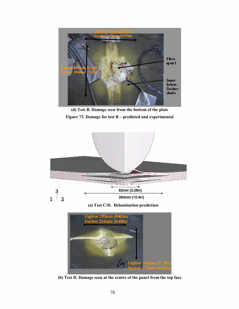
(d) Test B. Damage seen from the bottom of the plate

Figure 73. Damage for test B – predicted and experimental

(a) Test C/D. Delamination prediction

(b) Test D. Damage seen at the centre of the panel from the top face

76

(c) Test C/D. In-plane damage contours, showing E11 modulus

(d) Test D. Damage seen at the centre of the panel from the bottom face

Figures 74. Experimental and predicted damage – test C/D

77

Figure 75. Finite element, E11 and E22 modulus contours for test C/D.

TOP FACE (smooth) BOTTOM FACE lighter

discoloration darker

discoloration lighter

discoloration darker

discoloration (lxw) in mm (l x w) in mm (l x w) in mm (l x w) in mm

l w l w l w l w 340kg, Test A 124 117 151 16 69 90 143 192

454.5kg, Test B 147 131 152 165 74 132 142 186 682kg, Test C 250 146 215 174 122 143 152 184 682kg, Test D 206 144 164 170 110 112 147 145

Table 17. Delamination areas measured for tests A, B, C and D.

Figure 76. E33 modulus degradation for test A.

78

Figure 77. E33 modulus degradation for test B.

Figure 78. E33 modulus degradation for test C/D.

Note, that there may be potential discrepancies in the boundary conditions of the finite element analyses and those of the test. The plates where bolted down to the test fixture via holes drilled along the plate edges, see Figure 79. This boundary condition is not clamped but neither is it completely simply supported. However in the FE model, the simply supported boundary conditions were applied.

79

Figure 79. Showing a few of the holes along a plate edge used to attach the plates to the test fixture

4.4. CONCLUSION

The limited literature on impact modelling of composites is largely restricted to thin plates and do not include all failure modes. This work shows how a full 3d damage model is necessary to effectively model the behaviour of thicker plates under transverse loading.

It is observed that modelling 3d damage at the ply level and delamination reduces the contact force by up to 25% compared to the no-damage model but increases the contact time and out-of-plane displacement compared to the experiment. Thick plates with relatively few plies (in this case 9) simulated with a 2d damage model at the woven plies and cohesive layers at every inter-ply gave a highly over-predicted contact force. To reduce this it was necessary to model through-thickness damage at the woven layers. Inserting cohesive zones in between every ply may not be computationally reasonable for plates with many layers and modelling fewer cohesive layers can still provide satisfactory results as long as through-thickness damage is incorporated at the plies.

It was found that 3d damage model at the plies is the largest cause of reduction in contact force followed by the delamination model which also has the effect of stabilizing the contact behaviour through the absorption of some of the impact energy. Furthermore, the contact definition and the mesh density of the tup and plate collectively prove to be very influential in the contact force predictions.

80

5. CLOSING COMMENTS

To this day, there are no established composite models for predicting the behaviour and damage formation of composite plates under a dynamic load. Moreover, there is no validation work of large-scale woven roving composite plates using existing plane stress damage criteria. Most criteria are developed and tested on coupon-test scale specimens and although continuum damage mechanics approaches are now more prevalent, some of the models require complex test procedures and are limited to 2d damage modelling. The effect of full transverse material property degradation of thick composite plates has until now, not been tested under impact. The current work validates the application of a few of the most commonly used stress-based based criteria under in-plane loading and proposes a simple 3d damage model to include matrix, fibre and delamination damage prediction. The main findings are as follows:

The work on in-plane loading of large-scale plates has shown that a modified version of Hashin’s in-plane stress-based criteria appears to adequately model matrix and fibre damage of thick composite panels under in-plane loading conditions. However, Hashin’s 2d stress criteria largely over-predicted matrix and fibre damage under impact loading and Hashin’s 3d matrix damage criterion was also inappropriate as a damage initiation criterion under impact loading using solid elements. Modelling delamination with resin-rich layers between laminated plies embedded within shell

elements using 2d failure criteria, provides a reasonable, simple to use approximation of the behaviour of impacted plates.

▪ The maximum delamination areas are relatively well predicted however the sequence of delamination size through the thickness is not correctly modeled.

▪ The peak contact force although reduced compared to a no-damage model, is still generally notably higher than the test result.

Introducing a 3d gradually damaging model makes a substantial improvement to the damage size and location predictions and contact force, giving relatively good correlations with experiment. The matrix and fibre damage modelling at the woven plies is carried out using simple damage mechanics concepts requiring cyclic tests for material data. Cohesive elements are a good method of modelling delamination and improve contact force

predictions even if not all the cohesive regions are modelled as delaminating. These elements are not exempt from mesh density limitations. Where less than the full number of cohesive regions is modelled, it is important to include a

through-thickness damage model at the woven plies to effectively predict the contact force. A poor contact definition can be very influential on the results (particularly on the contact

force calculations). Related to this is mesh density. An experienced user can minimise the influence of mesh density on the results over a certain range of plate sizes, however mesh-independency is important with even larger scales than those considered in this work.

There are numerical limitations that prevent expansion of the model, the key being the inability to embed composite layers in solid elements in Abaqus/Explicit and the lack of knowledge of the element and integration point location in the user material subroutine. Despite this there are still controllable areas of the damage model which can undergo further development.

81

6. FURTHER DEVELOPMENT

Some of the most important areas to undergo further development are listed below:

Delamination

▪ Failure in compression under the influence of both normal and shear stresses ▪ Coupling of delamination and damage at woven layers ▪ Scale-independence.

– Mesh density issues when modelling large panels.

This model would involve implementing a coupled (linear or non-linear) damage relationship between the transverse stresses. Moreover, this would allow failure of the cohesive element in compression to be influenced not only by the transverse shear stresses but also by the normal transverse stress. Scale-dependency is still an issue with cohesive zone modelling, particularly when it comes to larger plates than the ones considered in this report.

3d damage model

▪ Strain rate dependence ▪ Coupled continuum damage mechanics model (CDM)

– Cyclic testing at various strain rates ▪ Scale-independence.

– Coupon test data is currently used for large panels – Mesh density issues when modelling large panels.

So far, the strain rate sensitivity of the composite has not been included at the woven ply level in any of the models in this study. In order to implement a gradually degrading model (a CDM model) that is also strain rate sensitive requires cyclic testing to be carried out under the high strain rates. There is a limit to how this can be achieved with normal tensile/compressive loading machines before having to turn to more complicated tests involving the split-Hopkinson bar. In addition, the CDM model currently used in this study does not couple the in-plane and through-thickness damage criteria. This is another area of much scope. Scaling issues need also to be addressed with regards to the use of data from small-coupon tests for the modelling of very large plates. Also, mesh density is an important issue when modelling these plates. Keeping the same element size for all plate sizes is unrealistic for very large plates and does not resolve the material property scaling issue.

Residual strength after impact

▪ Damaged state after impact (Explicit/VUMAT ▪ In-plane compression loading of damaged panel in Implicit/VUMAT

In order to obtain the residual strength of the panel after impact, the impacted panel must be loaded in-plane as with the intact panel, and thus strength values can be compared.

82

Modelling this test implicitly requires the transfer of all the state dependent variables from the damaged model in Abaqus/Explicit into Abaqus/Standard.

Full-scale modelling

The reason for seeking to develop a practical yet effective composite damage model is to eventually model the entire ship structure and enable the modelling of a structural component in more detail. This requires finer meshes and the mesh difference between the detailed portion and the surrounding material will cause time step issues. How to deal with this is another important area to be examined.

83

ACKNOWLEDGEMENTS

The authors are grateful for the financial support provided by the Office of Naval Research, Office of Naval Research Global and the Health and Safety Executive of the United Kingdom.

REFERENCES

1. Mouritz AP, Gellert E, Burchill P, Challis K. 2001. Composite Structures 53:21-41

2. Williams K.V., Vaziri R., Poursartip A. 2003. International Journal of Solids and Structures40:2267-300

3. Zhou G, Greaves LJ. 2000. In Impact Behaviour of Fibre-reinforced Composite Materials andStructures, ed. SR Reid, G Zhou, pp. 133-183. Woodhead Publishing Ltd

4. Elder DJ, Thomson RS, Nguyen MQ, Scott ML. 2004. Composite Structures 66:677-83

5. Boh JW, Louca LA, Choo YS, Mouring SE. 2005. Composites Part B: Engineering 36:427-38

6. Espinosa HD, Dwivedi S, Lu H-C. 2000. Computer Methods in Applied Mechanics andEngineering 183:259-90

7. Chen WH, Chang CM, Yeh JT. 1993. Computer Methods in Applied Mechanics and Engineering 109:315-29

8. Scheider I. 2001. Cohesive Model for Crack Propagation Analyses of Structures with Elastic-Plastic Material Behavior: Foundations and Implementation. GKSS Research Center, Geesthacht, Dept. WMS,

9. Camanho PP. 2003. Journal of Composite Materials 37:1415-38

10. Turon A, Davila CG, Camanho PP, Costa J. 2005. An Engineering Solution for using CoarseMeshes in the Simulation of Delamination With Cohesive Zone Models. Rep. NASA/TM-2005-213547, NASA,

11. Lemmen P, Meijer G-J, Rasmussen EA. Dynamic behavior of composite ship structures (DYCOSS) failure prediction tool. 2006. Ref Type: Unpublished Work

12. Hashin Z. 1980. Journal of applied mechanics 47:329-34

13. Chen H, Sun X. 1999. Composite Structures 47:711-7

14. Greene E. 1999. pp. 123-133. Annapolis: Eric Greene Associates

15. Rajbhandari SPSMLTRSHD. An approach to Modelling and predicting impact damage incomposite structures. ICAS 2002 Congress. 2002.Ref Type: Conference Proceeding

84

16. Swanson SR. 1993. Composite Structures 25:249-55

17. Rajbhandari SPSMLTRSHD. An approach to Modelling and predicting impact damage in composite structures. ICAS 2002 Congress. 2002. Ref Type: Conference Proceeding

18. Lesar DE. 2003. Composite Sail Advanced Project Report, Plan for sensitivity analyses of rate-dependent composite material properties in composite advanced sail structure. Rep. NSWCCD 652, NSWCCD,

19. Greenfield RJ. 1997. Dynamic tensile properties of woven glass fabric composites. Masters thesis. University of Delaware

20. Abaqus Users Reference Manual, Versions 6.4 and 6.5. 2005. Ref Type: Computer Program

21. Sun CT. Modelling high strain rate response and failure in polymeric composites. The 2nd Int. Conf. On Struc. Stability and Dynamics, Singapore. 2002. Ref Type: Conference Proceeding

22. Sun CT, Chen JL. 1989. Journal of Composite Materials 23:1009-20

23. Ladeveze P, Allix O, Daudeville L. 1991. IUTAM Symposium607-22

24. Ladeveze P, LeDantec E. 1992. Composites Science and Technology 43:257-67

25. Chaboche JL. 1988. Journal of applied mechanics 55:59-64

26. Iannucci L, Dechaene R, Willows M, Degrieck J. 2001. Computers & Structures 79:785-99

27. Camanho PP, Davila CG. 2002. Mixed-Mode Decohesion Finite Elements for the Simulation of Delamination in Composite Materials. Rep. NASA/TM-2002-211737, NASA,

28. Iannucci L. 2006. International Journal of Impact Engineering 32:1013-43

29. Matzenmiller A, Lubliner J, Taylor RL. 1995. Mechanics of Materials 20:125-52

30. Kollegal M. 2001. International journal of damage mechanics 10:301-23

31. Talreja R. 1985. Journal of Composite Materials 19:355-75

32. Sierakowski RL, Chaturverdi Sk. 1997. In Dynamic Loading and Characterization of fiber-reinforced composites, pp. 215. New York ; Chichester : Wiley

33. Davies GAO, Hitchings D, Zhou G. 1996. Composites Part A: Applied Science and Manufacturing 27:1147-56

34. Sutherland LS, Guedes Soares C. 2005. International Journal of Impact Engineering 31:1-23

35. Mouritz AP, Gallagher J, Goodwin AA. 1997. Composites Science and Technology 57:509-22

85

36. Goyal VK, Johnson ER, Davila CG, Jaunky N. 2002. An irreversible constitutive law for modelling the delamination process using interface elements. Rep. NASA/CR-2002-211758, ICASE Report No. 2002-25, NASA,

37. Camanho P P, Davila C.G. 2002. Mixed-Mode decohesion finite elements for the simulation of delamination in composite materials. Rep. NASA / TM-2002-211737,

38. Odegard G, Searles K, Kumosa M. 2001. Composites Science and Technology 61:2501-10

39. Mouritz AP. 1995. Composites Science and Technology 55:365-74

Published by the Health and Safety Executive 12/06




This report and the work it describes were funded by the Health and Safety Executive (HSE). Its contents, including any opinions and/or conclusions expressed, are those of the authors alone and do not necessarily reflect HSE policy.

RR520

www.hse.gov.uk

Documents

Damage modelling of large and small scale composite … and Safety Executive Damage modelling of large and small scale composite panels subjected to a low velocity impact H E Johnson