Damage Detection w Cvr1 - Copy

Integration of Bridge Damage Detection Concepts and Components

Final Report 2 of 3October 2013

Sponsored byIowa Highway Research Board(IHRB Project TR-636)Iowa Department of Transportation(InTrans Project 11-416)

Volume II: Acceleration-Based Damage Detection

About the BEC

The mission of the Bridge Engineering Center is to conduct research on bridge technologies to help bridge designers/owners design, build, and maintain long-lasting bridges.

Disclaimer Notice

The contents of this report reflect the views of the authors, who are responsible for the facts and the accuracy of the information presented herein. The opinions, findings and conclusions expressed in this publication are those of the authors and not necessarily those of the sponsors.

The sponsors assume no liability for the contents or use of the information contained in this document. This report does not constitute a standard, specification, or regulation.

The sponsors do not endorse products or manufacturers. Trademarks or manufacturers’ names appear in this report only because they are considered essential to the objective of the document.

Non-Discrimination Statement

Iowa’s Regent Universities do not discriminate on the basis of race, color, age, religion, national origin, sexual orientation, gender identity, genetic information, sex, marital status, disability, or status as a U.S. veteran. Inquiries can be directed to the Iowa State University Director of Equal Opportunity and Compliance, 3280 Beardshear Hall, (515) 294-7612.

Iowa Department of Transportation Statements

Federal and state laws prohibit employment and/or public accommodation discrimination on the basis of age, color, creed, disability, gender identity, national origin, pregnancy, race, religion, sex, sexual orientation or veteran’s status. If you believe you have been discriminated against, please contact the Iowa Civil Rights Commission at 800-457-4416 or Iowa Department of Transportation’s affirmative action officer. If you need accommodations because of a disability to access the Iowa Department of Transportation’s services, contact the agency’s affirmative action officer at 800-262-0003.

The preparation of this report was financed in part through funds provided by the Iowa Department of Transportation through its “Second Revised Agreement for the Management of Research Conducted by Iowa State University for the Iowa Department of Transportation” and its amendments.

The opinions, findings, and conclusions expressed in this publication are those of the authors and not necessarily those of the Iowa Department of Transportation.

Technical Report Documentation Page

1. Report No. 2. Government Accession No. 3. Recipient’s Catalog No.

IHRB Project TR-636

4. Title and Subtitle 5. Report Date

Integration of Bridge Damage Detection Concepts and Components

Volume II: Acceleration-Based Damage Detection

October 2013

6. Performing Organization Code

7. Author(s) 8. Performing Organization Report No.

Salam Rahmatalla, Charles Schallhorn, and Ghedhban Swadi InTrans Project 11-416

9. Performing Organization Name and Address 10. Work Unit No. (TRAIS)

Center for Computer-Aided Design

College of Engineering

University of Iowa

Iowa City, IA 52242

11. Contract or Grant No.

12. Sponsoring Organization Name and Address 13. Type of Report and Period Covered

Iowa Highway Research Board

Iowa Department of Transportation

800 Lincoln Way

Ames, IA 50010

Final Report 2 of 3

14. Sponsoring Agency Code

IHRB Project TR-636

15. Supplementary Notes

Visit www.intrans.iastate.edu for color pdfs of this and other research reports.

16. Abstract

In this work, a previously developed structural health monitoring (SHM) system was advanced toward a ready-for-implementation

system. Improvements were made with respect to automated data reduction/analysis, data acquisition hardware, sensor types, and

communication network architecture.

The objective of this part of the project was to validate/integrate a vibration-based damage-detection algorithm with the strain-

based methodology formulated by the Iowa State University Bridge Engineering Center. This report volume (Volume II) presents

the use of vibration-based damage-detection approaches as local methods to quantify damage at critical areas in structures.

Acceleration data were collected and analyzed to evaluate the relationships between sensors and with changes in environmental

conditions. A sacrificial specimen was investigated to verify the damage-detection capabilities and this volume presents a

transmissibility concept and damage-detection algorithm that show potential to sense local changes in the dynamic stiffness

between points across a joint of a real structure.

The validation and integration of the vibration-based and strain-based damage-detection methodologies will add significant value

to Iowa’s current and future bridge maintenance, planning, and management

17. Key Words 18. Distribution Statement

damage detection algorithm—failure-critical joints—local damage

quantification—sacrificial specimen—SHM—structural health

monitoring—temperature change effects—transmissibility ratios—

vibration-based detection

No restrictions.

19. Security Classification (of

this report)

20. Security Classification (of this

page)

21. No. of Pages 22. Price

Unclassified. Unclassified. 44 NA

Form DOT F 1700.7 (8-72) Reproduction of completed page authorized

THREE-VOLUME REPORT ABSTRACT

The Iowa Department of Transportation (DOT) started investing in research (through both the

Iowa Highway Research Board and the Office of Bridges and Structures) in 2003 to develop a

structural health monitoring (SHM) system capable of identifying damage and able to report on

the general operational condition of bridges. In some cases, the precipitous for these

developments has been a desire to avoid damage that might go unnoticed until the next biennial

inspection. Of specific and immediate concern was the state’s inventory of fracture-critical

structures.

The goal of this project was to bring together various components of recently-completed research

at Iowa’s Regent Universities with the following specific objectives:

Final development of the overall SHM system hardware and software

Integration of vibration-based measurements into current damage-detection algorithm

Evaluation and development of energy-harvesting techniques

The following three volumes of the final report cover the results of this project:

Volume I: Strain-Based Damage Detection, from the Iowa State University Bridge

Engineering Center, reviews information important to the strain-based SHM methodologies,

details the upgraded damage-detection hardware and software system, demonstrates the

application of the control-chart-based methodologies developed, and summarizes the results in

graphical and tabular formats.

Volume II: Acceleration-Based Damage Detection, from the University of Iowa Center for

Computer-Aided Design, presents the use of vibration-based damage-detection approaches as

local methods to quantify damage at critical areas in structures. Acceleration data were collected

and analyzed to evaluate the relationships between sensors and with changes in environmental

conditions. A sacrificial specimen was investigated to verify the damage-detection capabilities

and this volume presents a transmissibility concept and damage-detection algorithm that show

potential to sense local changes in the dynamic stiffness between points across a joint of a real

structure.

Volume III: Wireless Bridge Monitoring Hardware, from the University of Northern Iowa,

Electrical Engineering Technology, summarizes the energy harvesting techniques and prototype

development for a bridge monitoring system that uses wireless sensors. The functions and

performance of the developed system, including strain data, energy harvesting capacity, and

wireless transmission quality, are covered in this volume.

INTEGRATION OF BRIDGE DAMAGE DETECTION

CONCEPTS AND COMPONENTS

VOLUME II: ACCELERATION-BASED DAMAGE

DETECTION

Final Report 2 of 3

October 2013

Principal Investigator

Brent M. Phares, Director

Bridge Engineering Center, Iowa State University

Co-Principal Investigators

Salam Rahmatalla, Associate Professor

Civil and Environmental Engineering, Center for Computer-Aided Design, University of Iowa

Jin Zhu, Associate Professor

Electrical Engineering Technology, University of Northern Iowa

Ping Lu, Rating Engineer

Office of Bridges and Structures, Iowa Department of Transportation

Research Assistant and Postdoctoral Scholar

Charles Schallhorn and Ghedhban Swadi

Authors

Salam Rahmatalla, Charles Schallhorn, and Ghedhban Swadi

Sponsored by

the Iowa Highway Research Board and Iowa Department of Transportation

(IHRB Project TR-636)

Preparation of this report was financed in part

through funds provided by the Iowa Department of Transportation

through its Research Management Agreement with the

Institute for Transportation

(InTrans Project 11-416)

A report from

Center for Computer-Aided Design

College of Engineering, University of Iowa

Iowa City, IA 52242

Phone: 319-335-5722

v

TABLE OF CONTENTS

ACKNOWLEDGMENTS ............................................................................................................ vii

EXECUTIVE SUMMARY ........................................................................................................... ix

Problem Statement ............................................................................................................. ix

Objectives .......................................................................................................................... ix Research Description and Key Findings ............................................................................ ix Implementation Readiness and Conclusions .......................................................................x Implementation Benefits ......................................................................................................x

1. INTRODUCTION .......................................................................................................................1

1.1. Motivation .....................................................................................................................1

1.2. Background ...................................................................................................................2

1.3. Objective .......................................................................................................................3

2. THEORY .....................................................................................................................................4

3. ALGORITHM..............................................................................................................................6

4. TESTING ...................................................................................................................................10

4.1. Laboratory Testing ......................................................................................................10 4.2. Field Testing (US 30 Bridge) ......................................................................................15

5. CONCLUSIONS AND RECOMMENDATIONS ....................................................................28

REFERENCES ..............................................................................................................................31

APPENDIX A. COHERENCE FOR ADDITIONAL PAIRS OF SENSORS FOR

SACRIFICIAL SPECIMEN ..............................................................................................33

vi

LIST OF FIGURES

Figure 1. Outlined procedure for vibration-based damage-detection algorithm ..............................6 Figure 2. Process outline for damage state comparison and warning percentage ...........................8 Figure 3. Geometry and dimensions of connection specimen .......................................................10

Figure 4. Experimental layout of connection specimen .................................................................11 Figure 5. Connection specimen bolt removal plan: (a) damage scenario D0 (b) damage

scenario D3 ........................................................................................................................12 Figure 6. Coherence for pairs of sensors: (a) Sensors 2_1 (b) Sensors 2_3 ..................................13 Figure 7. Transmissibility diagrams of experimental connection specimen: (a) multiple

damage scenarios at Nodes 2 and 1 (b) multiple damage scenarios at Nodes 2 and 3 ......14 Figure 8. Percent warnings of manual impacts for multiple damage states compared to

baseline damage state for specimen connection 2_1 and 2_3 ............................................15

Figure 9. Typical time history of one-minute data file for traffic loading on bridge ....................16 Figure 10. Schematic layout of south span of US 30 bridge depicting locations of field

experiments ........................................................................................................................17

Figure 11. Sensor orientation for Section C...................................................................................17 Figure 12. Percent warnings for multiple days of traffic data compared to baseline day for

Section C ............................................................................................................................18 Figure 13. Absolute differences in average daily temperatures from the baseline day for

Section C ............................................................................................................................19

Figure 14. Sensor orientation for Section A ..................................................................................20 Figure 15. Percent warnings for multiple days of traffic data compared to baseline for

sensors at Section A: (a) vertical sensors (b) horizontal sensors .......................................21 Figure 16. Absolute differences in average daily temperatures from the baseline day for

Section A ............................................................................................................................22

Figure 17. Sensor orientation for sacrificial specimen ..................................................................23

Figure 18. Coherence for pair of Sensors 5 and 6 ..........................................................................24 Figure 19. Percent warnings of manual impacts for multiple damage states compared to

baseline damage state for the sacrificial specimen ............................................................25

Figure 20. Percent warnings of traffic data for multiple days compared to baseline day for

the sacrificial specimen ......................................................................................................26

Figure 21. Absolute differences in average daily temperatures from the baseline day for the

sacrificial specimen ............................................................................................................27

vii

ACKNOWLEDGMENTS

The authors would like to thank the Iowa Highway Research Board (IHRB) and Iowa

Department of Transportation (DOT) for sponsoring this research. The authors would also like

the thank Ahmad Abu-Hawash and many other members of the Iowa DOT Office of Bridges and

Structures for their continued support of this research.

ix

EXECUTIVE SUMMARY

Problem Statement

Infrastructure health conditions and monitoring have been an active area of research and

development due to the urgent demands for safer and longer-life structures. Many novel ideas

have been developed and have shown success using simulations and lab testing, but have

difficulties in detecting damage on large civil structures. The challenges are attributed to the

complexity of these structures and the presence of noise and environmental effects/interferences.

Objectives

The objective of this part of the project was to validate/integrate a vibration-based damage-

detection algorithm with the strain-based methodology formulated by the Iowa State University

Bridge Engineering Center. The proposed algorithm for vibration-based measurements was

based on localizing sensors around failure-critical joints and establishing transmissibility ratios.

The methodology was tested using laboratory experiments and field testing.

Research Description and Key Findings

The vibration-based algorithm was tested and validated as follows:

Laboratory experiments on a connection specimen using transient loading conditions

o Warning percentages detected, quantified, and located damage

o Percent warnings had difficulties in quantifying magnitudes of damage (could not exceed

100 percent)

Field testing on a sacrificial specimen that was geometrically similar to the laboratory

connection specimen

o Warning percentages detected damage under normal traffic loading

o Environmental effects (temperature, wind, construction, etc.) were believed to cause false

damage results

o Quantification of damage was unsuccessful due to variations caused by environmental

effects

Field testing of joints near the mid-span and quarter-span of a bridge girder

o Warning percentages were utilized on bridge connections directly with substantial

significance

o False damage was detected when significant changes in temperature occurred and during

construction of a trail under the bridge

x

Implementation Readiness and Conclusions

The transmissibility concept and damage-detection algorithm presented in this report

demonstrate the potential to sense local changes in the dynamic stiffness between points across a

joint of a real structure. Because the majority of failures occur at or near a connection, knowing

the changes in inertial properties of failure-critical joints on a bridge would greatly improve

detection capabilities and could prevent catastrophic failure.

This study showed that the presented algorithm is successful in experimental testing and that it

has great potential for application in field analysis.

Further investigation is required to expand the understanding of how temperature affects warning

percentages. Future work could entail temperature compensation within the damage-detection

algorithm or provision of supplemental temperature information to add redundancy to the

procedure.

Implementation Benefits

The validation and integration of the vibration-based and strain-based damage-detection

methodologies will add significant value to Iowa’s current and future bridge maintenance,

planning, and management.

1

1. INTRODUCTION

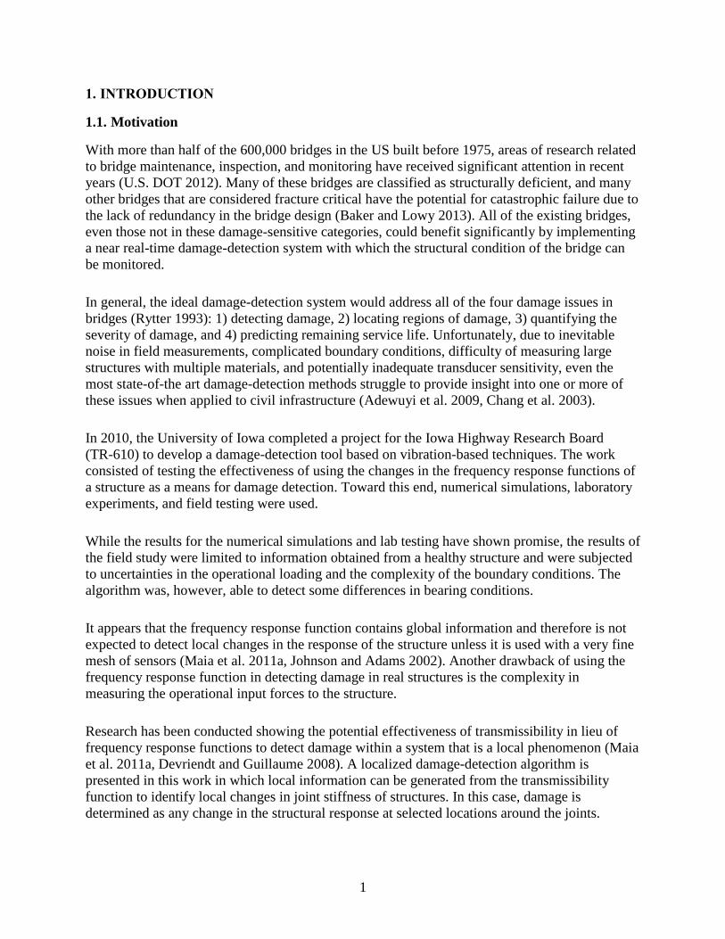
1.1. Motivation

With more than half of the 600,000 bridges in the US built before 1975, areas of research related

to bridge maintenance, inspection, and monitoring have received significant attention in recent

years (U.S. DOT 2012). Many of these bridges are classified as structurally deficient, and many

other bridges that are considered fracture critical have the potential for catastrophic failure due to

the lack of redundancy in the bridge design (Baker and Lowy 2013). All of the existing bridges,

even those not in these damage-sensitive categories, could benefit significantly by implementing

a near real-time damage-detection system with which the structural condition of the bridge can

be monitored.

In general, the ideal damage-detection system would address all of the four damage issues in

bridges (Rytter 1993): 1) detecting damage, 2) locating regions of damage, 3) quantifying the

severity of damage, and 4) predicting remaining service life. Unfortunately, due to inevitable

noise in field measurements, complicated boundary conditions, difficulty of measuring large

structures with multiple materials, and potentially inadequate transducer sensitivity, even the

most state-of-the art damage-detection methods struggle to provide insight into one or more of

these issues when applied to civil infrastructure (Adewuyi et al. 2009, Chang et al. 2003).

In 2010, the University of Iowa completed a project for the Iowa Highway Research Board

(TR-610) to develop a damage-detection tool based on vibration-based techniques. The work

consisted of testing the effectiveness of using the changes in the frequency response functions of

a structure as a means for damage detection. Toward this end, numerical simulations, laboratory

experiments, and field testing were used.

While the results for the numerical simulations and lab testing have shown promise, the results of

the field study were limited to information obtained from a healthy structure and were subjected

to uncertainties in the operational loading and the complexity of the boundary conditions. The

algorithm was, however, able to detect some differences in bearing conditions.

It appears that the frequency response function contains global information and therefore is not

expected to detect local changes in the response of the structure unless it is used with a very fine

mesh of sensors (Maia et al. 2011a, Johnson and Adams 2002). Another drawback of using the

frequency response function in detecting damage in real structures is the complexity in

measuring the operational input forces to the structure.

Research has been conducted showing the potential effectiveness of transmissibility in lieu of

frequency response functions to detect damage within a system that is a local phenomenon (Maia

et al. 2011a, Devriendt and Guillaume 2008). A localized damage-detection algorithm is

presented in this work in which local information can be generated from the transmissibility

function to identify local changes in joint stiffness of structures. In this case, damage is

determined as any change in the structural response at selected locations around the joints.

2

It is proposed that by placing the sensors strategically at failure-critical locations and by having a

reference sensor at a location where damage is unlikely to occur, it could be possible to detect,

locate, and quantify damage accurately for an entire structure utilizing localized damage-

detection principles.

1.2. Background

Local damage-detection techniques, such as acoustic approaches (i.e., ultrasonic, impact-echo,

tap test) and visual approaches (i.e., x-ray and gamma ray), have been proven to detect damage

accurately in the region very close to where the technology is deployed (Guo et al. 2005).

However, the logistics and cost associated with using these methods on civil infrastructures can

outweigh the benefits even for relatively small structures (Chang et al. 2003, Guo et al. 2005).

The concept of vibration-based damage-detection methods is that a change in dynamic

characteristics (mass, stiffness, or damping) can be detected by observing the associated change

in modal parameters such as natural frequency, mode shape, frequency response function (FRF),

and transmissibility (TR).

Although many methods have been investigated, few have shown success in field

implementation (Doebling et al. 1996), mainly due to the environmental effects (i.e.,

temperature, wind) (Chesne and Deraemaeker 2013). Works completed by Maia et al. (2001),

Maia et al. (2011b), and Weijtjens et al. (2013) show theoretically that transmissibility can be

used for more accurate and sensitive localized damage detection than frequency response

functions or mode shapes. These properties of transmissibility are discussed in Chapter 2.

Vibration-based damage-detection algorithms generally consist of placing numerous sensors to

obtain a global response to a structural system. Damage is then determined as any change in the

global response when compared to that from another time period. Again, it is proposed that by

placing the sensors strategically at failure-critical locations and by having a reference sensor at a

location where damage is unlikely to occur, it could be possible to detect, locate, and quantify

damage accurately for an entire structure utilizing localized damage-detection principles.

The main concept of the proposed algorithm comes from an understanding of acceleration-based

sensors and how the proximity from damage affects the signal collected by the sensor.

Acceleration-based sensors are expected to be sensitive to both the global and the local responses

of a system. If any damage is introduced into the system, the sensor should be able to detect the

changes in the dynamic response compared to the dynamic response from a previous time point.

The local response of the system would have a much larger effect on the signal and, therefore,

insight into damage location and quantification can be determined by the proximity of the

damage to the sensor.

3

1.3. Objective

For the vibration-based algorithm presented here, the theme is to show that vibration-based

damage-detection approaches are heavily investigated as global methods; however, little work

has been done to investigate their effectiveness as local damage-detection schemes, especially

for field applications.

The objective of this study is to use vibration-based damage-detection approaches as local

methods to quantify damage at critical areas in structures. Acceleration data were collected and

analyzed to evaluate the relationships between sensors and with changes in environmental

conditions. A sacrificial specimen was investigated to verify the damage-detection capabilities.

4

2. THEORY

The dynamic response of a structure is described as the influence or motion of the system due to

a non-static loading, such as an impulse load or forced vibration. Generally, the dynamic

response is a measure of the vibration of the system. Equations of motion have been commonly

used to solve for the displacements, velocities, and accelerations at determined locations, thus

resulting in the motion of a system due to an applied force. The equation of motion for a general

system is shown in Equation 1, where M is the mass matrix of the system, C is the damping

matrix, K is the stiffness matrix, is the nodal acceleration vector, is the nodal velocity

vector, u is the nodal displacement vector, and F(t) is the applied force vector.

(1)

In theory, the mass, damping, and stiffness matrices, as well as the applied force vector, are all

known quantities, therefore, Equation 1 is used to solve for the nodal displacements and their

time derivatives. Once these values are determined, the acceleration can be transformed from the

time domain to the frequency domain by applying a Fourier transform. Changes in the response

of the system can be seen in the time domain; however, they can be seen more easily in the

frequency domain as changes in the natural frequencies and mode shapes of the system.

For a single applied force, Equation 1 can be transformed to the frequency domain:

(2)

where D is the dynamic stiffness of the structure. For an undamped system, D can be represented

as:

(3)

where K represents the stiffness of the structure, M is the structure’s mass, and is the natural

frequency of the structure. Equation 2 can also be written as:

(4)

where H(s) is the inverse or pseudo-inverse of the dynamic stiffness matrix D, which is also

called the frequency response matrix, and can be calculated using the H1, H2, or Hv approaches

(Ewins 2000):

(5)

where is the cross-spectral density between the input force and the output displacement, and

is the auto-spectral density of the input force on the system.

5

(6)

For noisy data, the FRF can be calculated using the following function:

√ (7)

The transmissibility (Tkij) between two locations (i and j) on a structure as a result of an applied

force at location (k) can be defined as the ratio between the frequency response functions Hik(ω)

and Hjk(ω):

(8)

The transmissibility can also be defined directly from output-only responses, which is common

when examining a system where H cannot be determined. The ratio between the response at

position Xi and Xj directly gives the same relationship as Equation 8:

(9)

While it relates the motion information from two locations, the transmissibility function is

expected to be more sensitive to local changes when compared with the frequency response

function (H).

Ribeiro et al. (2000) similarly derived a general formulation of transmissibility. In the

formulation, it is defined that {F} is a vector of applied forces, {XU} is a vector of unknown

responses, {XK} is a vector of known responses, and [H] is the FRF matrix for the structure.

Similar to Equation 4, the relation between the applied forces and a set of responses is given by:

[ ]{ } { } (10)

[ ]{ } { } (11)

where [HKA] is the sub-matrix of [H] relating the known responses to the applied forces and

[HUA] is the sub-matrix of [H] relating the unknown responses to the applied forces. If [HKA] can

be inverted (e.g., #K ≥ #A), the following relationship is possible:

{ } [ ][ ] { } [

]{ } (12)

where [TA

KU] is the transmissibility matrix between the sets of coordinates K and U when the

forces are applied at coordinates A.

6

3. ALGORITHM

In this chapter, the vibration-based damage-detection algorithm developed for integration with

the Iowa State University (ISU) Bridge Engineering Center (BEC) damage-detection

methodology is presented. This procedure incorporates many characteristics similar to the

processes described previously, while adding novel aspects to data collection and analysis in

pursuit of an accurate localized vibration-based damage-detection algorithm that can be

implemented in field environments. The procedure is outlined in Figure 1.

Figure 1. Outlined procedure for vibration-based damage-detection algorithm

The algorithm begins with the proper installation of sensors. Throughout this project,

piezoelectric accelerometers were used for data collection. With an understanding of the

dynamics of the structure to measure, sensors could be placed at or near damage-critical

Implement sensors at damage critical locations (if known)

Gather acceleration data from a system or model

Transform data to frequency domain by FFT

Compare TR features for damage scenarios at regions of high coherence

Make decision whether or not damage has occurred

𝑠𝑖𝑔𝑛𝑎𝑙𝑑𝑟𝑖𝑓𝑡 𝑟𝑒𝑚𝑜𝑣𝑒𝑑 𝑠𝑖𝑔𝑛𝑎𝑙𝑜𝑟𝑖𝑔𝑖𝑛𝑎𝑙 𝑚𝑒𝑎𝑛𝑠𝑖𝑔𝑛𝑎𝑙 Remove drift from data by

Determine regions of high coherence/strong correlation

Normalize the data to be between 0.1 and 1

𝑇𝑅 20 log 0 𝑟𝑒𝑠𝑝𝑜𝑛𝑠𝑒 𝑠𝑖𝑔𝑛𝑎𝑙

𝑟𝑒𝑓𝑒𝑟𝑒𝑛𝑐𝑒 𝑠𝑖𝑔𝑛𝑎𝑙

Calculate transmissibility ratio (TR) by

Create features in TR at regions of high coherence

7

locations (i.e., connections, high-stress areas). Placing the sensors around these damage-critical

locations directly localizes the scope of the detection algorithm, thus improving the likelihood of

detecting small deficiencies.

With the sensors implemented in optimal locations, data could then be collected for any loading

scenario. Two types of loading scenarios were used in this project for analysis: transient

(impacts) and ambient (traffic). Depending on which loading scenario was applied, the data

points used for damage state sets within the algorithm were calculated differently. Individual

impacts were used from transient loading, and specified durations of the time history responses

(one-minute files) were used for ambient loading.

Depending on environmental conditions, sensor type, and other factors, drift may occur during

data collection and must be removed accordingly. Drift is removed by subtracting the mean

value from the original signal. It is most accurate when this calculation is carried out on a series

of small time steps per time history file (Phares et al. 2011).

The data is then transformed to the frequency domain using a fast-Fourier transform (FFT).

Given that the loadings will not be exactly the same experimentally, data normalization is used

such that an accurate representation of the transmissibility ratio (TR) can be determined. Without

this normalization, the ratio of the response signal to the reference signal could be distorted

based on loading conditions alone. Once the signals are normalized, the TR is calculated by

using the equation in Figure 1 above, where the log of the ratio is multiplied by 20, making dB

the units for TR.

The decision process for detecting damage is based on changes to the TR for a given pair of

sensors. Similar to the work completed by Maia et al. (2011a), the damage decision can be

calculated by discretizing the TR as a collection of features in which each feature is a range of

frequencies. It has been proposed that it is possible to investigate the effect of damage only on

certain frequency bands (Schulz et al. 1997), and Chesne and Deraemaeker (2013) state that it is

possible to increase the accuracy of the decision process by limiting these features. It is proposed

to look at the coherence between sensor signals to limit these features.

After obtaining the regions of high coherence, the comparison between damage states can be

conducted to decide if damage can be detected. The decision for detection is calculated as a

warning percentage for each set of data points. For purposes of clarification, two sets of data are

referred to in the discussion of the proposed algorithm: baseline set and comparison set. The

baseline set is comprised of all of the data (TR between pairs of sensors) collected for the healthy

or undamaged state and the comparison set is all of the data collected for a single damaged state.

There can be many comparison sets per analysis, but only one baseline set.

The warning percentage is an indication of the percent of data points (impacts or one-minute

files) in a given set that are statistically different from the baseline set of data points and

difference from the baseline set is classified as damage.

8

The calculation to determine if a point is statistically different from the baseline set is shown in

Figure 2.

Figure 2. Process outline for damage state comparison and warning percentage

The mean and standard deviation of the baseline set of TR for a given pair of sensors are

calculated and used to normalize the baseline set. This normalization is completed to account for

the magnitude differences of the TR for each feature (frequency range). A threshold variable is

created to allow a buffer between data points. This buffer accounts for the variations in TR due

to noise, environmental conditions, etc. The comparison data are then normalized by the same

parameters as the baseline set normalization.

By utilizing the regions of high coherence, the ranges of frequencies (features) are used to

discretize the sets of normalized data. For each feature, the difference between the normalized

comparison set and the mean of the normalized baseline set is calculated, thus returning a vector

of values for each feature. The summation of these values for the length of the vector is

compared with the threshold variable to determine if a warning is detected for the impact or one-

minute file.

Calculate mean (μ) and standard deviation (σ) of baseline set

𝑏𝑎𝑠𝑒𝑙𝑖𝑛𝑒 𝑠𝑒𝑡𝑛𝑜𝑟𝑚𝑎𝑙𝑖𝑧𝑒𝑑 𝑖 𝑏𝑎𝑠𝑒𝑙𝑖𝑛𝑒 𝑠𝑒𝑡 𝑖 𝜇𝑏𝑎𝑠𝑒𝑙𝑖𝑛𝑒 𝑠𝑒𝑡

𝜎𝑏𝑎𝑠𝑒𝑙𝑖𝑛𝑒 𝑠𝑒𝑡

Normalize baseline set by

𝑡ℎ𝑟𝑒𝑠ℎ𝑜𝑙𝑑 𝜎𝑏𝑎𝑠𝑒𝑙𝑖𝑛𝑒 𝑠𝑒𝑡 ∗ 𝑃 Threshold variable created by

where P is a specified number and remains constant for each damage state

𝑐𝑜𝑚𝑝𝑎𝑟𝑖𝑠𝑜𝑛 𝑠𝑒𝑡𝑛𝑜𝑟𝑚𝑎𝑙𝑖𝑧𝑒𝑑 𝑖 𝑐𝑜𝑚𝑝𝑎𝑟𝑖𝑠𝑜𝑛 𝑠𝑒𝑡 𝑖 𝜇𝑏𝑎𝑠𝑒𝑙𝑖𝑛𝑒 𝑠𝑒𝑡

𝜎𝑏𝑎𝑠𝑒𝑙𝑖𝑛𝑒 𝑠𝑒𝑡

Normalize comparison set by

𝑐𝑜𝑚𝑝𝑎𝑟𝑖𝑠𝑜𝑛 𝑠𝑒𝑡𝑛𝑜𝑟𝑚𝑎𝑙𝑖𝑧𝑒𝑑 𝜇𝑛𝑜𝑟𝑚𝑎𝑙𝑖𝑧𝑒𝑑 𝑏𝑎𝑠𝑒𝑙𝑖𝑛𝑒 𝑠𝑒𝑡

𝑓𝑒𝑎𝑡𝑢𝑟𝑒𝑠

> 𝑡ℎ𝑟𝑒𝑠ℎ𝑜𝑙𝑑

Warning is detected if

𝑁𝑢𝑚𝑏𝑒𝑟 𝑜𝑓 𝑓𝑖𝑙𝑒𝑠 𝑜𝑟 𝑖𝑚𝑝𝑎𝑐𝑡𝑠 𝑡ℎ𝑎𝑡 𝑑𝑒𝑡𝑒𝑐𝑡 𝑤𝑎𝑟𝑛𝑖𝑛𝑔𝑐𝑜𝑚𝑝𝑎𝑟𝑖𝑠𝑜𝑛 𝑠𝑒𝑡

𝑇𝑜𝑡𝑎𝑙 𝑛𝑢𝑚𝑏𝑒𝑟 𝑜𝑓 𝑓𝑖𝑙𝑒𝑠 𝑜𝑟 𝑖𝑚𝑝𝑎𝑐𝑡𝑠𝑐𝑜𝑚𝑝𝑎𝑟𝑖𝑠𝑜𝑛 𝑠𝑒𝑡∗ 100

Percent warning for each damage state is calculated by

9

Collecting these warnings for multiple impacts or files leads to the warning percentage, which

give a more accurate representation of the damage state. These warning percentages are proposed

to not only detect damage, but to also offer quantification between damage states.

10

4. TESTING

4.1. Laboratory Testing

4.1.1. Equipment

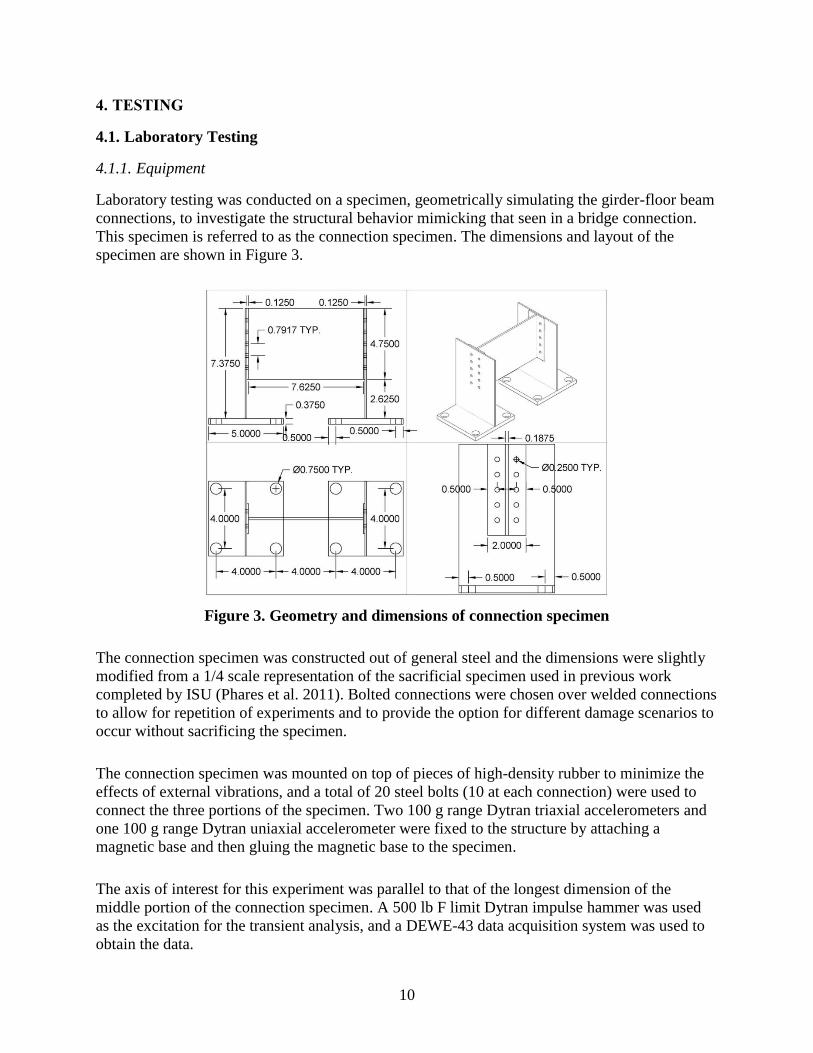
Laboratory testing was conducted on a specimen, geometrically simulating the girder-floor beam

connections, to investigate the structural behavior mimicking that seen in a bridge connection.

This specimen is referred to as the connection specimen. The dimensions and layout of the

specimen are shown in Figure 3.

Figure 3. Geometry and dimensions of connection specimen

The connection specimen was constructed out of general steel and the dimensions were slightly

modified from a 1/4 scale representation of the sacrificial specimen used in previous work

completed by ISU (Phares et al. 2011). Bolted connections were chosen over welded connections

to allow for repetition of experiments and to provide the option for different damage scenarios to

occur without sacrificing the specimen.

The connection specimen was mounted on top of pieces of high-density rubber to minimize the

effects of external vibrations, and a total of 20 steel bolts (10 at each connection) were used to

connect the three portions of the specimen. Two 100 g range Dytran triaxial accelerometers and

one 100 g range Dytran uniaxial accelerometer were fixed to the structure by attaching a

magnetic base and then gluing the magnetic base to the specimen.

The axis of interest for this experiment was parallel to that of the longest dimension of the

middle portion of the connection specimen. A 500 lb F limit Dytran impulse hammer was used

as the excitation for the transient analysis, and a DEWE-43 data acquisition system was used to

obtain the data.

11

For all of the damage scenarios, a sampling rate of 5,000 samples per second was used. All of the

programs required for the damage-detection algorithm were written in MATLAB, in which the

data gathered by the DEWE-43 system was easily converted to the appropriate file format for

use.

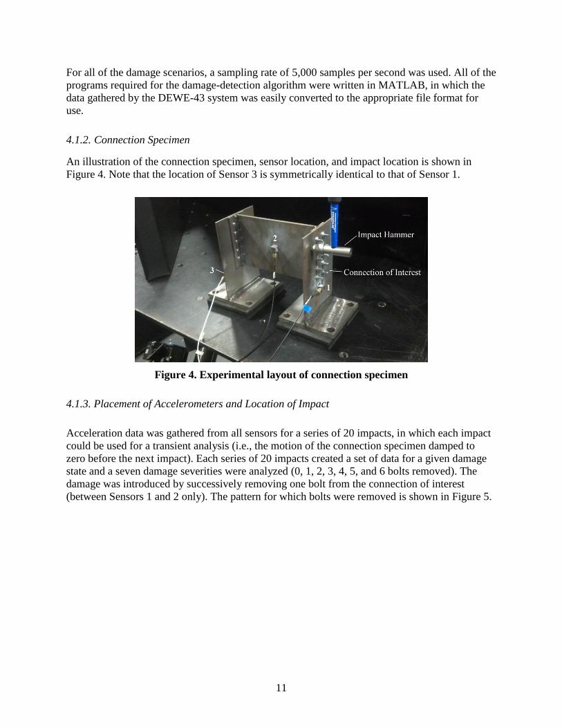
4.1.2. Connection Specimen

An illustration of the connection specimen, sensor location, and impact location is shown in

Figure 4. Note that the location of Sensor 3 is symmetrically identical to that of Sensor 1.

Figure 4. Experimental layout of connection specimen

4.1.3. Placement of Accelerometers and Location of Impact

Acceleration data was gathered from all sensors for a series of 20 impacts, in which each impact

could be used for a transient analysis (i.e., the motion of the connection specimen damped to

zero before the next impact). Each series of 20 impacts created a set of data for a given damage

state and a seven damage severities were analyzed (0, 1, 2, 3, 4, 5, and 6 bolts removed). The

damage was introduced by successively removing one bolt from the connection of interest

(between Sensors 1 and 2 only). The pattern for which bolts were removed is shown in Figure 5.

12

Figure 5. Connection specimen bolt removal plan: (a) damage scenario D0 (b) damage

scenario D3

The data acquired for this experiment was then used to calculate the TR for symmetric sides of

the connection specimen (i.e., the TR between Sensors 1 and 2 and between Sensors 2 and 3).

The notation for each damage scenario is D#_Ref_Res, where # is the number of bolts removed,

Ref refers to the reference node, and Res refers to the response node. For example, D2_2_1

corresponds to the damage scenario with 2 bolts removed, with Node 2 as the reference signal

and Node 1 as the response signal. The coherence is shown in Figure 6, and the regions of high

coherence used for the analysis was decided as the ranges from 30 to 215 Hertz and 325 to 410

Hertz. The averaged TR over 20 impacts of Nodes 1, 2, and 3 for each damage scenario is shown

in Figure 7.

(a) (b)

13

Figure 6. Coherence for pairs of sensors: (a) Sensors 2_1 (b) Sensors 2_3

-4

-3

-2

-1

0

1

2

3

0 50 100 150 200 250 300 350 400 450 500

20

Lo

g 10

TR

Frequency (Hz)

D0_2_1 D1_2_1 D2_2_1 D3_2_1 D4_2_1 D5_2_1 D6_2_1

0

0.1

0.2

0.3

0.4

0.5

0.6

0.7

0.8

0.9

1

0 50 100 150 200 250 300 350 400 450 500

Co

he

ren

ce

Frequency (Hz)

(a)

(b)

14

Figure 7. Transmissibility diagrams of experimental connection specimen: (a) multiple

damage scenarios at Nodes 2 and 1 (b) multiple damage scenarios at Nodes 2 and 3

It is apparent that the damage caused by removing bolts in a connection changes the

transmissibility between sensors adjacent to the damage significantly, while the transmissibility

between sensors away from the damage are nearly unaffected. Given that damage is clearly

detected and located for these pairs of transmissibility, the feature extraction algorithm was used

for validation. The percent warning for each damage state is shown in Figure 8.

-4

-3

-2

-1

0

1

2

3

0 50 100 150 200 250 300 350 400 450 500

20

Lo

g 10

TR

Frequency (Hz)

D0_2_1 D1_2_1 D2_2_1 D3_2_1 D4_2_1 D5_2_1 D6_2_1

-4

-3

-2

-1

0

1

2

3

0 50 100 150 200 250 300 350 400 450 500

20

Lo

g 10

TR

Frequency (Hz)

D0_2_3 D1_2_3 D2_2_3 D3_2_3 D4_2_3 D5_2_3 D6_2_3

(a)

(b)

15

See Figure 4 for sensor locations

Figure 8. Percent warnings of manual impacts for multiple damage states compared to

baseline damage state for specimen connection 2_1 and 2_3

The feature extraction algorithm clearly identifies damage between Sensors 1 and 2 (tall blue

bars in Figure 8) for all damage scenarios and quantification of damage is seen by the increasing

warning percentage. No damage is detected between Sensors 2 and 3 (short red bars in Figure 8),

which is expected given that the properties of transmissibility allow for local detection. Based on

the results from this experiment, the algorithm shows great potential for detecting, quantifying,

and locating damage within a system.

4.2. Field Testing (US 30 Bridge)

4.2.1. Equipment

To implement the presented algorithm in the field, a variety of equipment and materials were

utilized to obtain the dynamic characteristics of the bridge. The data acquisition system was

constructed by ISU, in which six additional sensor adaptors were installed to account for the

accelerometers to be implemented on-site. Six Brüel and Kjaer 0.5 g range DeltaTron uniaxial

seismic accelerometers were used for a better signal-to-noise ratio, as well as to increase the

sensitivity of the damage-detection capabilities significantly.

Each sensor was attached to a base plate or bracket (for directionality purposes, and an L-bracket

was used in some locations) and the base was then epoxied to the structure. To protect the sensor

from the environment, and in case of detachment, each sensor was wrapped in plastic wrap, foam

strips, and duct tape. For some sensors, spray-on foam insulation was used around the base to

help weatherize the sensor.

16

Data files consisting of one-minute intervals of traffic data for all sensors were transmitted to the

University of Iowa (UI) via a secure file transfer protocol (ftp) site hosted by ISU, allowing for

remote access to and usage of the data. A typical data file for acceleration is shown in Figure 9.

Figure 9. Typical time history of one-minute data file for traffic loading on bridge

Each one-minute files was then compiled (by day or 1,440 files) in MATLAB to then be used in

the presented algorithm, which was written as a series of MATLAB programs. A total of 35 days

of data, non-consecutive, were used for the analysis of Section C (Figures 10 and 11) and the

sacrificial specimen (Figure 17) starting on September 13, 2012 and ending on November 6,

2012. Thirty-eight days of data, non-consecutive, were used for the analysis of Section A

(Figures 10 and 14) beginning on November 27, 2012 and ending on March 11, 2013.

All of the field experiments for this project were conducted under the south span of the US 30

Bridge. A schematic of the bridge and the experiment locations are shown in Figure 10.

-0.30

-0.20

-0.10

0.00

0.10

0.20

0.30

0 10 20 30 40 50 60

Acc

ele

rati

on

(g)

Time (seconds)

17

Figure 10. Schematic layout of south span of US 30 bridge depicting locations of field

experiments

4.2.2. Section C

Data were collected for a beam-girder connection at Section C, shown in Figure 11.

Figure 11. Sensor orientation for Section C

The purpose of this data acquisition and analysis was to demonstrate the likelihood of false

damage detection, as no damage was created intentionally at this joint, and damage was not

expected to occur throughout the duration of the project.

18

Following the same procedure as the connection specimen (Section 4.1.2), the acceleration data

from the traffic vibrations were used to determine the TR between the pair of sensors shown

above.

In lieu of having damage states for comparison, each day of data (set of 1,440 one-minute files)

was used for comparison, and a warning percentage was calculated based on these evaluations.

To account for some of the noise and nonlinearity of the system, a buffer was introduced such

that percentages less than the buffer limit (10 percent) were still considered acceptable or non-

damaged. As shown in Figure 12, false damages were detected for a few days near October 10

and all of the days after October 27.


Figure 12. Percent warnings for multiple days of traffic data compared to baseline day for

Section C

The dashed vertical lines and damage labels refer to the days when damage was created in the

sacrificial specimen, which is discussed later. Initial investigation of the false damages showed

an association between percent warning and temperature. The temperature is averaged over the

same 24 hour period for the comparison to the baseline data, and each comparison day’s average

temperature is shown in Figure 13.

0.00

10.00

20.00

30.00

40.00

50.00

60.00

70.00

80.00

90.00

100.00

1 2 3 4 5 6 7 8 9 10 11 12 13 14 15 16 17 18 19 20 21 22 23 24 25 26 27 28 29 30 31 32 33 34

Pe

rce

nt

War

nin

g (%

)

Day for Damage Comparison

Sep 26 Oct 10 Oct 24 Sep 13 Nov 6

Damage 3 Damage 1 Damage 2

19

Figure 13. Absolute differences in average daily temperatures from the baseline day for

Section C

When comparing the percent warnings for Section C with the absolute differences in temperature

for these days, it’s apparent that these false damage warnings occur during significant changes in

temperature. The exception to this, and the justification for further investigation, is the

significant change in temperature between October 10 and October 27 that did not alter the

percent warning significantly.

The association between percent warning and temperature changes suggests that for any

significant change in temperature between days (or during the same day), a similarly significant

change occurs within the warning percentage. Further investigation is required to better

understand the relationship between temperature and damage quantification. Overall, the

presented algorithm was successful at detecting damage for days in which temperatures remained

near stationary; therefore, this algorithm could benefit from supplementary temperature

information to negate false warnings.

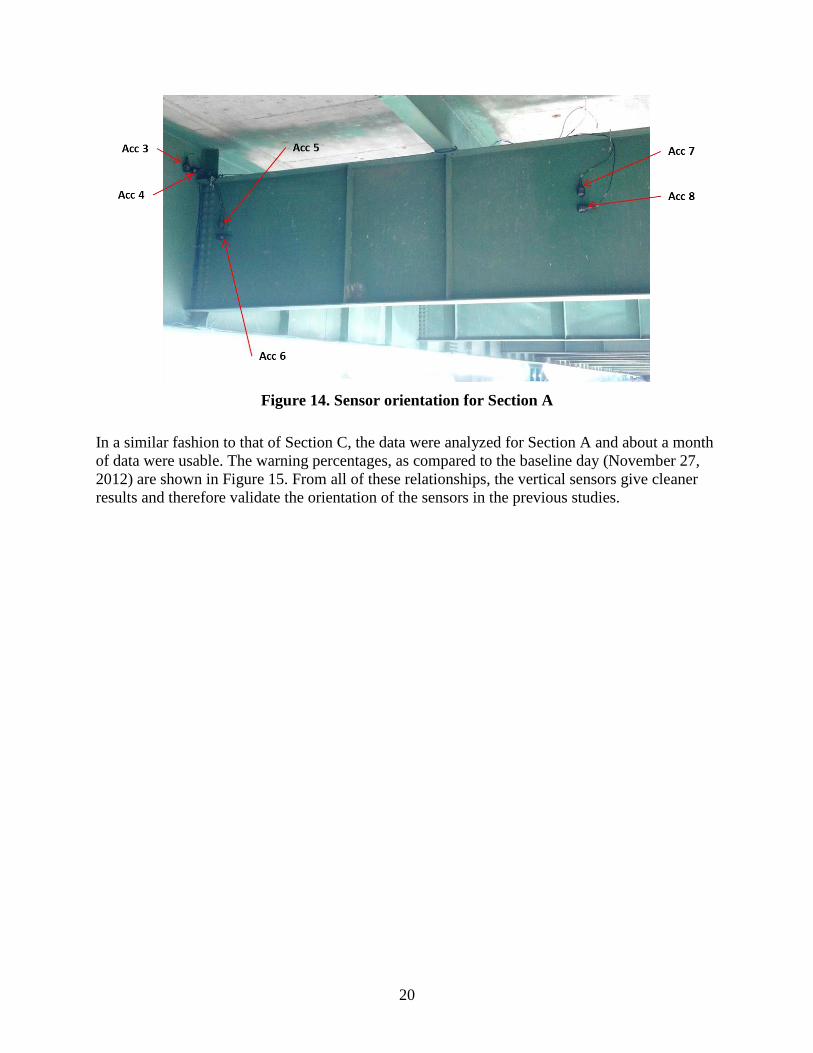
4.2.3. Section A

Similar to Section C, data were collected at Section A to investigate the likelihood of false

warnings, as well as explore temperature effects and sensor orientation. Due to the complexity

and nonlinearity of the loading and response of the bridge, a parametric study was completed to

determine the ideal orientation of the sensors. The layout and labels of each of the sensors used

for this study are shown in Figure 14. The odd-numbered sensors were vertical and the even-

numbered sensors were normal to the web of the north girder.

0.00

5.00

10.00

15.00

20.00

25.00

30.00

35.00

1 2 3 4 5 6 7 8 9 1011121314151617181920212223242526272829303132333435

Ab

solu

te D

iffe

ren

ce in

Te

mp

era

ture

fr

om

Bas

elin

e D

ay (

°F)


Steel Concrete AirSep 26 Oct 10 Oct 24 Sep 13 Nov 6


20

Figure 14. Sensor orientation for Section A

In a similar fashion to that of Section C, the data were analyzed for Section A and about a month

of data were usable. The warning percentages, as compared to the baseline day (November 27,

2012) are shown in Figure 15. From all of these relationships, the vertical sensors give cleaner

results and therefore validate the orientation of the sensors in the previous studies.

21


Figure 15. Percent warnings for multiple days of traffic data compared to baseline for

sensors at Section A: (a) vertical sensors (b) horizontal sensors

0.00

10.00

20.00

30.00

40.00

50.00

60.00

70.00

80.00

90.00

100.00

1 2 3 4 5 6 7 8 9 10111213141516171819202122232425262728293031323334353637

Pe

rce

nt

War

nin

g (%

)


7_5 7_3 5_3

Nov 27 Mar 11

0.00

10.00

20.00

30.00

40.00

50.00

60.00

70.00

80.00

90.00

100.00

1 2 3 4 5 6 7 8 9 10111213141516171819202122232425262728293031323334353637

Pe

rce

nt

War

nin

g (%

)


8_6 8_4 6_4

Nov 27 Mar 11

(a)

(b)

22

Temperature effects were also investigated, and, similar to Section C, false damage detection

could be related to significant changes in temperature. When comparing Figure 16 to the warning

percentages, some of the false damages are related to significant changes in temperature, while

others are not. Therefore, further investigation is needed to understand the temperature effect on

this damage-detection algorithm.

Figure 16. Absolute differences in average daily temperatures from the baseline day for

Section A

Overall, damage is clearly detected for days when the temperature remained stationary.

Therefore, this algorithm is proving successful in field applications.

4.2.4. Sacrificial Specimen

To further validate the presented algorithm in field testing, the sacrificial specimen (Phares et al.

2011) was utilized to determine if fatigue cracks could be detected through normal traffic

loading. The sacrificial specimen used for this work is shown in Figure 17, as are the labels and

locations of the accelerometers implemented on the specimen.

0.00

5.00

10.00

15.00

20.00

25.00

30.00

1 3 5 7 9 11 13 15 17 19 21 23 25 27 29 31 33 35 37

Ab

solu

te D

iffe

ren

ce in

Te

mp

era

ture

fr

om

Bas

elin

e D

ay (

°F)


Steel Concrete Air

Nov 27 Mar 11

23

Figure 17. Sensor orientation for sacrificial specimen

All of the sensors were installed to measure vertical acceleration due to the loading being

transmitted vertically to the specimen from the bridge via the strut. The direction that had the

largest motion was vertical; therefore, the signal strength in the vertical direction was optimal.

As traffic crossed the bridge, the vibration of the girders would be transferred to the sacrificial

specimen via the strut.

These vibrations were captured by the sensors implemented on the specimen and then

transmitted to UI for analysis. As the decision process dictates, a percent warning for each day

was determined to ascertain how different the compared signals were from the baseline. To

account for some of the noise and nonlinearity of the system, a buffer was introduced such that

percentages less than the buffer limit (10 percent) were still considered acceptable or non-

damaged.

Data were collected for two weeks for the undamaged sacrificial specimen to create a baseline

set. Of these two weeks of data, one day (24 hour period from midnight to midnight) was

designated as the baseline day (September 14, 2012), with which all other days of data were

compared. After the initial two weeks of data collection, damage was introduced into the

sacrificial specimen by an accelerated fatigue method. This process included removing the strut

(so as to not cause damage to the bridge), placing a shaker on the specimen, vibrating the

specimen at its natural frequency until a fatigue crack initiates or propagates a certain amount,

and then replacing the strut.

24

An additional two weeks of data were collected for this damage state, and then damage was

propagated again. This cycle continued until three damage states were completed and eight

weeks of data were collected.

On the days when damage was created or propagated, a transient analysis was conducted on the

sacrificial specimen without the strut attached to investigate any effect the removal and

replacement of the strut might have on the damage-detection process. These transient analyses

were conducted by impacting the specimen with the hammer used in the laboratory tests.

Each test consisted of approximately 50 impacts to obtain statistical significance. Two tests were

conducted on the same day that damage was created: one before the damage and one after the

damage. Figure 18 shows the coherence between Sensors 5 and 6, and the regions of high

coherence used for the analysis was set as the range from 15 to 35 Hertz.

Figure 18. Coherence for pair of Sensors 5 and 6

The coherence for the other pairs of sensors investigated showed very similar values; therefore,

these plots are included in the appendix rather than here. Figure 19 shows the results of these

transient analyses as compared to the 50 impacts taken before Damage 1.

0

0.1

0.2

0.3

0.4

0.5

0.6

0.7

0.8

0.9

1

0 10 20 30 40 50 60 70 80 90 100

Co

he

ren

ce

Frequency (Hz)

D1a_5_6 D1b_5_6 D2a_5_6 D2b_5_6 D3_5_6

25


Figure 19. Percent warnings of manual impacts for multiple damage states compared to

baseline damage state for the sacrificial specimen

The notation used in this figure is as follows: the number (1, 2, or 3) represents the damage state,

the lowercase letter “a” represents the 50 impacts directly after the damage for that damage state,

and the lowercase letter “b” represents the 50 impacts directly before the next damage state (two

weeks after D#a).

The expectation from these results was that each separate damage state should give a similar

percent warning (i.e., D1a should be similar to D1b) and that the percent warning should increase

with damage (i.e., D1b should be smaller than D2a). As expected, damage is clearly detected (all

damage states are above the 10 percent buffer limit), and damage is nearly quantified in that D2

is larger than D1. Because the percent warning cannot exceed 100 percent, any difference or

quantification between D2 and D3 is not visible when comparing results to the baseline data.

After showing that the algorithm works on the sacrificial specimen for manual impacts, the

algorithm was then used to determine whether or not damage could be detected by using traffic

data. This traffic data was gathered in parallel with the transient analyses, providing two weeks

of data for each damage state. Due to some unforeseen error in transmission, days in which the

majority of the one-minute files were missing were not included in the analysis, which explains

why there are not 14 days for each damage state shown in the results. Figure 20 shows the

percent warnings for each day compared to the baseline. As shown, the healthy days are within

the acceptable buffer of 10 percent, and all other days clearly detect damage (>10 percent) in the

sacrificial specimen.

0.00

10.00

20.00

30.00

40.00

50.00

60.00

70.00

80.00

90.00

100.00

D1a D1b D2a D2b D3

Pe

rce

nt

War

nin

g (%

)

Damage State for Damage Comparison

Oct 10 Oct 10 Oct 24 Sep 26 Oct 24

Damage 1

Damage 3

Damage 2

26


Figure 20. Percent warnings of traffic data for multiple days compared to baseline day for

the sacrificial specimen

Damage quantification was unsuccessful for this analysis due to the inconsistencies in the

percent warnings. However, initial investigation showed an association between percent warning

and temperature changes. The temperature is averaged over the same 24 hour period for the

comparison to the baseline data, and each comparison day’s average temperature is shown in

Figure 21.

0.00

10.00

20.00

30.00

40.00

50.00

60.00

70.00

80.00

90.00

100.00

1 2 3 4 5 6 7 8 9 10 11 12 13 14 15 16 17 18 19 20 21 22 23 24 25 26 27 28 29 30 31 32 33 34

Pe

rce

nt

War

nin

g (%

)


5_6 6_7 6_8Sep 26 Oct 10 Oct 24 Sep 13 Nov 6


27

Figure 21. Absolute differences in average daily temperatures from the baseline day for the

sacrificial specimen




understand the relationship between temperature and damage quantification.

0.00

5.00

10.00

15.00

20.00

25.00

30.00

35.00

1 2 3 4 5 6 7 8 9 1011121314151617181920212223242526272829303132333435

Ab

solu

te D

iffe

ren

ce in

Te

mp

era

ture

fr

om

Bas

elin

e D

ay (

°F)


Steel Concrete Air

Sep 26 Oct 10 Oct 24 Sep 13 Nov 6


28

5. CONCLUSIONS AND RECOMMENDATIONS

The transmissibility concept and damage-detection algorithm presented in this report

demonstrate the potential to sense local changes in the dynamic stiffness between points across a

joint of a real structure. Because the majority of failures occur at or near a connection, knowing

the changes in inertial properties of failure-critical joints on a bridge would greatly improve

detection capabilities and could prevent catastrophic failure.

The vibration-based algorithm was tested and validated as follows:

Laboratory experiments on a connection specimen using transient loading conditions

o Warning percentages detected, quantified, and located damage

o Percent warnings had difficulties in quantifying magnitudes of damage (could not exceed

100 percent)

Field testing on a sacrificial specimen that was geometrically similar to the laboratory

connection specimen

o Warning percentages detected damage under normal traffic loading

o Environmental effects (temperature, wind, construction, etc.) were believed to cause false

damage results

o Quantification of damage was unsuccessful due to variations caused by environmental

effects

Field testing of joints near the mid-span and quarter-span of a bridge girder

o Warning percentages were utilized on bridge connections directly with substantial

significance

o False damage was detected when significant changes in temperature occurred and during

construction of a trail under the bridge

This study showed that the presented algorithm is successful in experimental testing and that it

has great potential for application in field analysis.




understand the relationship between temperature and damage quantification. Overall, the

presented algorithm was successful at detecting damage for days in which temperatures remained

near stationary; therefore, this algorithm could benefit from supplementary temperature

information to negate false warnings.

With further investigation to expand the understanding of how temperature affects warning

percentages, future work could entail temperature compensation within the damage-detection

algorithm or provision of supplemental temperature information to add redundancy to the

procedure.

29

It should also be noted that during the investigation of the field specimen and bridge,

construction of a trail occurred directly underneath the bridge. Although the exact start date of

construction is unknown, it is reasonably estimated that construction equipment was being used

from around October 23 through the middle of November. This construction equipment added

noise and ambient vibrations to the entire system (bridge, sacrificial specimen, and surrounding

area) that could account for the false damage readings seen in Figures 19, 20, and 12. Although it

is not definite that this construction is the cause for the false damage detections, the vibrations

were significant enough to warrant discussion.

The validation and integration of the vibration-based and strain-based damage-detection

methodologies will add significant value to Iowa’s current and future bridge maintenance,

planning, and management.

31

REFERENCES

Adewuyi, A. P., Wu, Z., and Serker, N. H. M. K. (2009). “Assessment of Vibration-Based

Damage Identification Methods Using Displacement and Distributed Strain

Measurements.” Structural Health Monitoring, August 2009. 8(6), 443-461.

Baker, M., and Lowy, J. (2013). “Thousands of Bridges at Risk of Freak Collapse.” Associated

Press, Seattle.

Chang, P. C., Flatau, A., and Liu, S. C. (2003). “Health Monitoring of Civil Infrastructure.”

Journal of Structural Health Monitoring, 2(3), 257-267.

Chesne, S., and Deraemaeker, A. (2013). “Damage Localization Using Transmissibility

Functions: A Critical Review.” Mechanical Systems and Signal Processing, 28, 569-584.

Devriendt, C., and Guillaume, P. (2008). “Identification of Modal Parameters from

Transmissibility Measurements.” Journal of Sound and Vibration, 314, 343-356.

Doebling, S. W., Farrar, C. R., Prime, M. B., and Shevitz, D. W. (1996). Damage Identification

and Health Monitoring of Structural and Mechanical Systems from Changes in their

Vibration Characteristics: A Literature Review. Los Alamos National Laboratory Report.

Ewins, D. J. (2000). Modal Testing: Theory, Practice and Application, Second Edition,

Philadelphia: Research Studies Press Ltd. Print.

Guo, G. Q., Xiaozhai, Q., Dong, W., and Chang, P. (2005). “Local Measurement for Structural

Health Monitoring.” Earthquake Engineering and Engineering Vibration, 4(1), 165-172.

Johnson, T. J. and Adams, D. E. (2002) “Dynamic Transmissibility as a Differential Indicator of

Structural Damage” Journal of Vibration and Acoustics., American Society of

Mechanical Engineering. Vol. 124, No. 4, 634-641.

Maia, N. M. M., Almeida, R. A. B., Urgueira, A. P. V., and Sampaio, R. P. C. (2011a). “Damage

Detection and Quantification Using Transmissibility.” Mechanical Systems and Signal

Processing, 25, 2475-2483.

Maia, N. M. M., Urgueira, A. P. V., and Almeida, R. A. B. (2011b). Whys and Wherefores of

Transmissibility. Vibration Analysis and Control – New Trends and Developments, Dr.

Francisco Beltran-Carbajal (Ed.), ISBN: 978-953-307-433-7, InTech.

Maia, N. M. M., Silva, J. M. M., and Ribeiro, A. M. R. (2001). “The Transmissibility Concept in

Multi-Degree-of-Freedom Systems.” Mechanical and Signal Processing, 15, 129-137.

Phares, B. M., Wipf, T. J., Lu, P., Greimann, L., and Pohlkamp, M. (2011). An Experimental

Validation of a Statistical-Based Damage-Detection Approach. Bridge Engineering

Center, Iowa State University, Ames, Iowa. January 2011.

Ribeiro, A. M. R., Silva, J. M. M., and Maia, N. M. M. (2000). “On the Generalization of the

Transmissibility Concept.” Mechanical and Signal Processing, 14, 29-35.

Rytter, A. (1993). Vibration Based Inspection of Civil Engineering Structures. PhD thesis,

Department of Building and Structural Engineering, Aalborg University, Denmark.

Schulz, M. J., Abdelnaser, A. S., Pai, P. F., Linville, M. S., and Chung, J. (1997). Detecting

Structural Damage Using Transmittance Functions. International Modal Analysis

Conference, Orlando, Florida. 638-644.

U.S. DOT. (2012). Deficient Bridges by State and Highway System 2012. Last accessed October

4, 2013. Available at: www.fhwa.dot.gov/bridge/nbi/no10/defbr12.cfm.

Weijtjens, W., De Sitter, G., Devriendt, C., and Guillaume, P. (2013). “Relative Scaling of Mode

Shapes Using Transmissibility Functions.” Mechanical Systems and Signal Processing,

40, 269-277.

33

APPENDIX A. COHERENCE FOR ADDITIONAL PAIRS OF SENSORS FOR

SACRIFICIAL SPECIMEN

0

0.1

0.2

0.3

0.4

0.5

0.6

0.7

0.8

0.9

1

0 10 20 30 40 50 60 70 80 90 100

Co

he

ren

ce

Frequency (Hz)

D1a_5_7 D1b_5_7 D2a_5_7 D2b_5_7 D3_5_7

0

0.1

0.2

0.3

0.4

0.5

0.6

0.7

0.8

0.9

1

0 10 20 30 40 50 60 70 80 90 100

Co

he

ren

ce

Frequency (Hz)

D1a_5_8 D1b_5_8 D2a_5_8 D2b_5_8 D3_5_8

34

0

0.1

0.2

0.3

0.4

0.5

0.6

0.7

0.8

0.9

1

0 10 20 30 40 50 60 70 80 90 100

Co

he

ren

ce

Frequency (Hz)

D1a_6_7 D1b_6_7 D2a_6_7 D2b_6_7 D3_6_7

0

0.1

0.2

0.3

0.4

0.5

0.6

0.7

0.8

0.9

1

0 10 20 30 40 50 60 70 80 90 100

Co

he

ren

ce

Frequency (Hz)

D1a_6_8 D1b_6_8 D2a_6_8 D2b_6_8 D3_6_8

Documents

Damage Detection w Cvr1 - Copy