Embed Size (px)
Citation preview

SESM 16-02
Damage and Restoration of Water
Supply Systems in an Earthquake
Sequence
By
Keith A. Porter
July 2016
Structural Engineering and Structural Mechanics Program
Department of Civil Environmental and Architectural Engineering
University of Colorado
UCB 428
Boulder, Colorado 80309-0428

– ii –
Abstract Damage to potable water supply systems profoundly affects society after earthquakes. For at least
25 years, engineers have performed computerized risk analyses of earthquake damage to water -
supply systems to estimate earthquake damage and restoration. A new stochastic simulation model
is offered here that employs a fairly traditional loss-estimation approach, but proposes to extend
the state of the art in three notable ways: (1) It deals with lifeline interaction by directly modeling
how individual repairs are slowed by limitations in so-called upstream lifelines and other
prerequisites. (2) It quantifies damage and restoration over the entire earthquake sequence, i.e.,
considering damage in the mainshock, aftershocks, and afterslip. (3) It offers an empirical model
of service restoration as a function of the number of pipeline repairs performed (as opposed to
more rigorous, but computationally demanding, hydraulic analysis). A fourth novelty is that it
offers a procedure to adjust Hazus-MH estimates of restoration to account for an earthquake
sequence, lifeline interaction, and corrects for Hazus’ default assumptions about the number of
available repair crews.
The model is exercised on two Bay Area water supply systems subjected to a hypothetical but
highly realistic earthquake sequence initiating with a Mw 7.0 mainshock on the Hayward Fault in
the eastern San Francisco Bay Area, plus 16 aftershocks of M 5 or greater, occurring over 17
months after the mainshock. The model quantifies system damage, recovery, delays due to fuel
and other lifeline limitations, and setbacks in restoration because of aftershocks. It estimates the
benefit of a fuel-management plan and an accelerated pipe-replacement plan, in terms of
accelerated restoration of service. The model is validated several ways for each of the two case-
study water supply systems and seems reasonable. One water utility anticipates using it to target
vulnerable segments of its system for accelerated pipe replacement.
Acknowledgments The author thanks Jacob Walsh and James Wollbrinck of the San Jose Water Company, along with
Andrea Chen, Clifford Chan, Xavier Irias, Roberts McMullin, Devina Ojascastro, and Serge
Terentieff of the East Bay Municipal Utility District for their help constructing and testing the
models presented here and peer reviewing the report. Thanks especially to Jamie Jones of the U.S.
Geological Survey for preparing most of the maps presented here and for her patience and
assistance with various spatial analyses.

– iii –
Contents Abstract ........................................................................................................................................... ii
Acknowledgments........................................................................................................................... ii
1. Introduction ................................................................................................................................. 1
1.1 How water supply is important in an earthquake.................................................................. 1
1.2 Study objectives .................................................................................................................... 2
1.3 Organization of report ........................................................................................................... 3
2. Literature review ......................................................................................................................... 3
2.1 A panel approach to estimating water supply impacts .......................................................... 3
2.2 Analytical approaches to estimating water supply impacts .................................................. 4
2.3 Damageability of buried pipe................................................................................................ 5
2.3.1 Vulnerability and fragility functions .............................................................................. 5
2.3.2 Hazus-MH, M. O’Rourke and Ayala (1993), and Honneger and Eguchi (1992) .......... 5
2.3.3 Eidinger (2001) .............................................................................................................. 6
2.3.4 T. O’Rourke et al. (2014) ............................................................................................... 8
2.3.5 M. O’Rourke (2003) ...................................................................................................... 9
2.4 Tasks and methods to repair leaks and breaks .................................................................... 10
2.5 Time to repair pipe leaks and breaks .................................................................................. 13
2.6 Serviceability of water supply............................................................................................. 17
2.7 Lifeline interaction .............................................................................................................. 19
2.8 Pipeline damage in afterslip ................................................................................................ 25
2.9 Measuring loss of resilience................................................................................................ 26
3. Methodology ............................................................................................................................. 26
3.1 Overview of the methodology............................................................................................. 26
3.2 Vulnerability model ............................................................................................................ 27
3.2.1 What is a vulnerability model? .................................................................................... 27
3.2.2 Selecting a vulnerability model for a pipeline network ............................................... 28
3.3 Damage analysis (number of repairs required) ................................................................... 32
3.3.1 What is a damage analysis? ......................................................................................... 32
3.3.2 Applying the damage analysis to a water supply system ............................................. 32
3.3.3 Breaks or leaks? ........................................................................................................... 33
3.3.4 Degraded vulnerability? ............................................................................................... 33
3.4 Restoration model ............................................................................................................... 34
3.4.1 What is a lifeline restoration model? ........................................................................... 34

– iv –
3.4.2 Number of services lost because of earthquake ........................................................... 34
3.4.3 Number of services restored by the nth repair .............................................................. 34
3.4.4 Repair resources and repair rate with lifeline interaction ............................................ 36
3.4.5 Ordering lifelines to avoid circular lifeline interaction................................................ 39
3.4.6 Rate-limiting factors for lifeline repairs....................................................................... 41
3.4.7 Depicting lifeline interaction with an influence diagram............................................. 43
3.5 Measuring water supply resilience...................................................................................... 46
3.6 Optional stochastic simulation methodology ...................................................................... 47
3.6.1 Simulation of earthquake excitation ............................................................................ 47
3.6.2 Simulation of pipeline vulnerability ............................................................................ 47
3.6.3 Simulation of damage to buried pipeline ..................................................................... 48
3.6.4 Simulation of restoration.............................................................................................. 49
3.7 Accounting for afterslip and aftershocks ............................................................................ 51
3.8 Adjusting Hazus’ lifeline restoration model ....................................................................... 51
3.8.1 Why one might need to adjust the restoration curves offered by Hazus-MH .............. 51
3.8.2 Adjusting Hazus’ estimates of lifeline restoration to account for repair crews ........... 52
3.8.3 Accounting for lifeline interaction in Hazus-MH ........................................................ 53
3.8.4 Accounting for aftershocks in Hazus-MH ................................................................... 53
3.9 Mitigation options ............................................................................................................... 54
3.9.1 Fuel plan....................................................................................................................... 54
3.9.2 Pipe replacement .......................................................................................................... 55
3.10 Summary of the methodology ........................................................................................... 55
4. Case study 1: San Jose Water Company ................................................................................... 56
4.1 San Jose Water Company asset definition .......................................................................... 56
4.2 San Jose Water Company hazard analysis .......................................................................... 60
4.3 San Jose Water Company damage analysis ........................................................................ 63
4.4 San Jose Water Company restoration analysis ................................................................... 71
4.5 Validation of San Jose Water Company restoration analysis ............................................. 74
4.5.1 Cross validation with SJWC’s internal damage estimate ............................................ 74
4.5.2 Validation against Northridge, Kobe, and South Napa earthquakes............................ 74
4.5.4 Cross validation with Hazus-MH................................................................................. 75
4.6 San Jose Water Company under ideal-world conditions .................................................... 76
4.7 Effect of lifeline interaction and consumable limits ........................................................... 77
5. Case study 2: East Bay Municipal Utility District .................................................................... 77

– v –
5.1 East Bay Municipal Utility District asset definition ........................................................... 77
5.2 EBMUD hazard analysis..................................................................................................... 80
5.3 EBMUD damage analysis ................................................................................................... 84
5.4 EBMUD restoration analysis .............................................................................................. 90
5.5 Validation of EBMUD damage and recovery estimates ..................................................... 93
5.5.1 Cross validation with EBMUD internal damage estimates ......................................... 93
5.5.2 Comparison with EBMUD judgment, Northridge, Kobe, and Napa restoration ......... 94
5.5.3 Cross validation with Hazus-MH................................................................................. 94
5.6 Effect of lifeline interaction and consumable limits on EBMUD....................................... 95
6 Performance of other water utilities based on Hazus-MH ......................................................... 95
7. Conclusions ............................................................................................................................. 100
7.1 Summary ........................................................................................................................... 100
7.2 Research needs .................................................................................................................. 101
8. References cited ...................................................................................................................... 102

– vi –
Index of Figures
Figure 1. ShakeOut water restoration in MMI VIII or higher, where the vertical axis denotes
fraction of customers receiving service (Jones et al. 2008) ............................................................ 4
Figure 2. A. Tolerable fault offset vs. unanchor length in continuous pipe (O'Rourke 2003, citing
Kennedy et al., 1977), and B. Tolerable fault offset versus pipe-fault intersection angle in
segmented pipe (O'Rourke 2003, citing O’Rourke and Trautmann, 1981) .................................. 10
Figure 3. Lund and Schiff (1991) pipeline damage survey instrument ........................................ 13
Figure 4. Hazus-MH model of serviceability. Hazus uses the curve labeled “NIBS.” ................. 18
Figure 5. A. Restoration of water service after the 1994 Northridge earthquake and B. After the
1995 Kobe earthquake .................................................................................................................. 19
Figure 6. Illustration of afterslip ................................................................................................... 25
Figure 7. Eidinger (2001) pipe liquefaction vulnerability for K2 = 1.0, mean and 90% bounds .. 30
Figure 8. Parametric restoration curves with Kobe and Northridge experience ........................... 36
Figure 9. Repair times based on data from Schiff (1988): (A) all repairs (B) excluding repairs to
large diameter pipe ........................................................................................................................ 37
Figure 10. Lifeline interaction influence diagram ........................................................................ 44
Figure 11. Alternate lifeline interaction influence diagram, showing value outcomes ................ 45
Figure 12. Above-ground petroleum tank ..................................................................................... 55
Figure 13. SJWC system map ....................................................................................................... 58
Figure 14. SJWC pipe quantities by diameter............................................................................... 60
Figure 15. SJWC system map with mainshock peak ground velocity .......................................... 62
Figure 16. SJWC system map with liquefaction probability ........................................................ 62
Figure 17. SJWC system map with landslide probability ............................................................. 63
Figure 18. SJWC system map with M 6.4 Mountain View aftershock PGV contours (increments
of 0.08 m/sec)................................................................................................................................ 63
Figure 19. Buried water pipeline damage heatmap for the Hayward Fault mainshock in SJWC's
service area.................................................................................................................................... 67
Figure 20. Buried water pipeline damage heatmap for Cupertino M 6.4 aftershock in SJWC's
service area.................................................................................................................................... 68
Figure 21. Buried water pipeline damage heatmap for entire the Hayward Fault earthquake
sequence in SJWC's service area .................................................................................................. 69
Figure 22. Simulated repairs in SJWC buried pipelines in Hayward Fault mainshock ................ 70
Figure 23. Simulated repairs in SJWC buried pipelines in Cupertino M 6.4 aftershock .............. 70
Figure 24. Simulated repairs in SJWC buried pipelines in Hayward Fault sequence .................. 71
Figure 25. Simulated repair timeline of San Jose Water Company, with and without fuel
management plan .......................................................................................................................... 73
Figure 26. Simulated service availability of San Jose Water Company, with and without fuel
management plan .......................................................................................................................... 73
Figure 27. Comparison of the present model with that of Hazus-MH, as applied to SJWC ........ 76
Figure 28. Benefit of replacing AC and CI pipe with ductile iron: A) repairs remaining versus time
and B) services available versus time ........................................................................................... 77
Figure 29. EBMUD system map (red) with dividing line (yellow) to approximately separate pipe
and services east and west of the East Bay Hills .......................................................................... 79
Figure 30. EBMUD water supply system with mainshock peak ground velocities ..................... 81
Figure 31. EBMUD water supply system with mainshock liquefaction probability .................... 82
– vii –
Figure 32. Mainshock landslide probability near EBMUD service area ...................................... 82
Figure 33. EBMUD system with fault .......................................................................................... 83
Figure 34. EBMUD water supply system with Oakland M 5.42 aftershock PGV contours ........ 83
Figure 35. Buried water pipeline damage heatmap for the Hayward Fault mainshock in EBMUD’s
service area.................................................................................................................................... 88
Figure 36. Buried water pipeline damage heatmap for the most-damaging aftershock in EBMUD’s
service area.................................................................................................................................... 89
Figure 37. Buried water pipeline damage heatmap for the entire Hayward Fault sequence in
EBMUD’s service area ................................................................................................................. 90
Figure 38. EBMUD repair-crew availability ................................................................................ 91
Figure 39. Initial serviceability east and west of the East Bay Hills ............................................ 91
Figure 40. EBMUD restoration curves in the Hayward Fault sequence: (A) under as-is conditions,
showing service east and west of East Bay Hills, and (B) under several conditions, total for the
system ........................................................................................................................................... 92
Figure 41. EBMUD repair progress in the Hayward Fault sequence (A) under as-is conditions,
showing repair progress east and west of East Bay Hills, and (B) under several conditions, total
for the system ................................................................................................................................ 93
Figure 42. Cross validation of EBMUD restoration with Hazus-MH .......................................... 95
Figure 43. Water restoration (A) according to initial Hazus-MH calculations (B) after adjusting for
repair-crew availability and lifeline interaction, (C) after all utilties have implemented a fuel plan,
and (D) ideal-world conditions. Curves in B, C, and D use the more-detailed case-study
calculations for Contra Costa, Alameda, and Santa Clara counties instead of Hazus-MH. ....... 100

– viii –
Index of Tables
Table 1. Eidinger (2001) pipe vulnerability factors K1 and K2....................................................... 8
Table 2. Water pipeline repair tasks.............................................................................................. 11
Table 3. Repair times for water supply pipeline damage in the 1987 Whittier Narrows Earthquake
(Schiff 1988) ................................................................................................................................. 15
Table 4. Tabucchi et al. (2010) LADWP repair productivity estimates ....................................... 16
Table 5. Hazus-MH (2012) estimates of repair time per pipe repair ............................................ 17
Table 6. Lifeline interaction matrix in the Loma Prieta earthquake (after Nojima and Kameda
1991) ............................................................................................................................................. 21
Table 7. The San Francisco Lifelines Council’s (2014) lifeline system interdependencies matrix
....................................................................................................................................................... 24
Table 8. Comparison of criteria for selecting pipeline vulnerability functions ............................ 29
Table 9. Tentative interdependency u-values ............................................................................... 42
Table 10. Uncertain pipe-repair duration ...................................................................................... 49
Table 11. SJWC pipe construction, associated with Eidinger (2001) vulnerability functions ..... 59
Table 12. Hayward Fault earthquake sequence ............................................................................ 61
Table 13. Mainshock mean damage estimate in San Jose Water Company buried pipeline ........ 64
Table 14. Estimated number of leaks and breaks in SJWC buried pipeline in the Hayward Fault
sequence ........................................................................................................................................ 65
Table 15. Total leaks and breaks by day ....................................................................................... 65
Table 16. Repair rate in Hayward Fault sequence in San Jose Water Company buried pipeline, by
material.......................................................................................................................................... 66
Table 17. SJWC lost service-days................................................................................................. 74
Table 18. Hazus-MH estimate of Santa Clara County loss of water supply................................. 75
Table 19. EBMUD pipe construction, associated with Eidinger (2001) vulnerability functions . 79
Table 20. EBMUD pipe quantities by diameter ............................................................................ 80
Table 21. Hayward Fault mean damage estimate in EBMUD buried pipeline............................. 85
Table 22. Estimated number of leaks plus breaks in EBMUD buried pipeline in the Hayward Fault
sequence ........................................................................................................................................ 85
Table 23. Total EBMUD leaks plus breaks by day....................................................................... 86
Table 24. Repair rate in Hayward Fault sequence in EBMUD buried pipeline, by material ....... 86
Table 25. Repair rate in Hayward Fault sequence in EBMUD buried pipeline, by diameter....... 87
Table 26. EBMUD lost service-days ............................................................................................ 93
Table 27. Hazus-MH estimate of Contra Costa and Alameda County loss of water supply ........ 95
Table 28. Repair-crew adjustment factors q/q0 for Bay Area buried water supply pipeline
restoration...................................................................................................................................... 96
Table 29. Hazus-MH unadjusted estimate of water service restoration ....................................... 97
Table 30. Hazus-MH-based estimate of water service restoration after adjusting for repair crew
availability, lifeline interaction, but with no fuel plan. Santa Clara, Alameda, and Contra Costa
Counties are as calculated in case studies without a fuel plan. ..................................................... 98
Table 31. Hazus-MH-based estimate of water service restoration after adjusting for repair crew
availability, lifeline interaction, and with a fuel plan. Santa Clara, Alameda, and Contra Costa
Counties are as calculated in case studies. .................................................................................... 99
Table 32. Hazus-MH-based estimate of water service restoration after adjusting for repair crew
availability, lifeline interaction, with a fuel plan and emergency generators and fuel at all pumping

– ix –
stations. Santa Clara, Alameda, and Contra Costa Counties are as calculated in case studies under
ideal-world conditions................................................................................................................... 99

– 1 –
1. Introduction
1.1 How water supply is important in an earthquake People need potable water for daily life, businesses need water for air conditioning, and water is
an input to many natural and manufactured products and processes. Damage to the water supply
system can contribute greatly to the life-safety and economic consequences of an earthquake, as
illustrated by the economic analyses performed for the 2008 ShakeOut scenario (Rose et al. 2011).
In that study, the authors found that water supply interruption in a hypothetical M 7.8 earthquake
on the Southern San Andreas Fault could realistically result in $24 billion in business interruption
losses, a figure that represents more than one third of the $68 billion in total business interruption
losses and 13% of the total of property damage plus business interruption. A potable water supply
is crucial to carrying on life in residences, businesses, government, hospitals, and other critical
care facilities. Long aware of the importance of water supply and the potential for earthquakes to
interrupt water supply, earthquake experts recommend that homes and businesses have enough
water to provide for one gallon per person, per day after a major earthquake to last at least 3 days
and ideally for 2 weeks.
Loss of water supply in that hypothetical earthquake would also contribute substantially to the fire
damage to property, which itself could realistically account for $65 billion of the $113 billion in
property losses (Scawthorn 2008). The ShakeOut scenario is not a worst-case earthquake: the
rupture it deals with has a mean recurrence interval of 150 years, and it has been 300 years since
the last rupture. Furthermore, the fire simulation assumes mild winds rather than the fast, hot, dry,
Santa Anas that commonly blow in the fall and notoriously fan wildfires.
These earlier estimates, while particular to the ShakeOut, reflect a general truth: earthquake
damage to water supply systems in the United States (and elsewhere) threaten the health, safety,
and welfare of the population, possibly more than earthquake damage to any other utility or other
element of the built environment in part because repairs are so costly and time consuming. More
narrowly, earthquakes pose a nearly existential financial threat to any water supply util ity in a
seismically active region. If a utility cannot deliver water it cannot collect revenues, which can
threaten its ability to make payroll. Every water utility in earthquake country may be at risk.
The Hayward Fault earthquake sequence scenario examines among other things the potential for
damage to water supply systems in the San Francisco Bay Area from a large, but not exceedingly
rare, M 7.05 earthquake on the Hayward Fault in the eastern Bay Area. Earthquakes damage water
supply systems and the damage causes other problems, such as for firefighting. The 1906 San
Francisco earthquake damaged so much of that city’s potable water supply system that pressure
dropped too low for firefighters to fight the fires that eventually destroyed much of the city. The
moment-magnitude (Mw) 6.9 1989 Loma Prieta earthquake caused at least 761 breaks to water
mains and services in pipelines of various materials (Lund and Schiff 1991). The loss of
firefighting water supply in the San Francisco Marina District contributed to the fire that damaged
seven structures, destroying four buildings containing 33 apartments and flats (Scawthorn et al.
1991). Cast iron, steel, ductile iron, plastic and copper pipes all broke both within and outside areas
of liquefaction and other ground failure. The Mw 6.0 2014 South Napa earthquake caused 163
pipeline breaks in the City of Napa (SPA Risk LLC 2014).

– 2 –
The largest total number of breaks and the highest break rate (breaks per mile) in the 1989
earthquake occurred in cast iron pipe subjected to liquefaction-induced ground failure, but other
materials also broke, including ductile iron, PVC, and steel. Pipe broke in 1989 in places that were
not known to have experienced ground failure, so that damage has been attributed to ground strain
associated with wave passage, especially Rayleigh surface waves. There was no observed
liquefaction damage to buried pipeline in Napa in the 2014 earthquake, reinforcing the idea that
wave passage alone can damage buried pipe. Even the modest Mw 4.0 Piedmont, California
earthquake of 17 Aug 2015 caused 9 breaks to buried cast iron water supply pipe in the San
Francisco East Bay (Bay City News 18 Aug 2015).
Repairs to an earthquake-damaged water supply system can take months or more. Each break can
take as little as two hours to repair, but large numbers of breaks and larger pipes can take much
longer. The 30-inch water main that broke near the UCLA campus at 3:30 PM on Tuesday July
29, 2014, took almost 5 days, until 11:00 AM Sunday, August 3 to repair (LADWP 2014). During
an earthquake sequence, with many simultaneous breaks, repairs take longer for many reasons.
Some of these are:
1. When a pressure zone loses pressure because of many breaks, it can be necessary to repair
breaks closer to the source (i.e., nearer the tank, reservoir, etc.) before one discovers breaks
farther from the source.
2. Similarly, it may be necessary to repair damage to a pumping plant, reservoir, or regulator
before damage in the downstream pipeline network can be addressed.
3. Water districts have an upper limit to their ability to field and manage multiple repair crews
operating in parallel, even when the crews are from outside contractors or from water
districts that provide mutual aid.
4. Limited supplies of repair resources such as spare pipe, clamps, fuel, and repair crews.
5. Damage to other systems—electrical and gas, for example—can hinder pipeline repair, and
in some cases those repairs can cause pipeline damage. Coordination with other agencies
can conceivably idle repair crews.
6. Aftershocks can hinder repair efforts because they pose an ongoing safety threat to repair
crews. They can also cause new damage or aggravate earlier breaks.
1.2 Study objectives
In this work, I attempt to depict a realistic outcome of the damage and restoration of water supply
in the Hayward Fault earthquake sequence. I review available models of earthquake-induced
pipeline damage and repair, propose one for use in the scenario earthquake sequence, and apply it
to the water supply systems of the San Jose Water Company and the East Bay Municipal Utility
District. These two systems were chosen because they are strongly shaken, are affected by the
mainshock and by aftershocks, and were willing to share their system maps. The maps were shared
under strict requirements of confidentiality, so map details are not available here.
This study supplements conventional loss estimation by examining the detailed activities involved
in discovering and repairing water pipeline damage. It identifies steps in the repair process that

– 3 –
rely on other lifelines, to inform a new model of the effects of lifeline interaction to delay water
service repairs and restoration.
This study focuses on damage and repair of buried water pipe, which tends to dominate the effort
to restore water supply. It considers damage resulting from wave passage, liquefaction,
landsliding, and fault offset. It ignores earthquake damage to other elements in the water-supply
system, including raw water aqueducts, tanks, tunnels, canals, valves, and reservoirs. The decision
to focus this study on buried pipelines without including other critical facilities such as tanks,
reservoirs, tunnels, etc., seems reasonable, since a majority of water utilities have implemented
seismic improvement programs (SIP) that, for the most part, focused on seismically retrofitting
their tanks, reservoirs, etc. but not their old distribution pipelines. As such, old distribution
pipelines, as an asset class, present the most significant seismic vulnerability for most water
utilities, since for the most part smaller diameter distribution mains were not replaced with seismic-
resistant mains because it simply wasn’t economically feasible to replace them all as part of a SIP.
This study does not address restoration of water utilities’ customer base or the change in demand
for water as homes and businesses relocate because of building damage or other reasons.
1.3 Organization of report
This section has summarized the nature of the problem and presented the study objectives. Section
2 presents relevant literature. The methodology and rationale for its selection are presented in
Section 3. Section 4 presents a case study using the San Jose Water Company’s water supply buried
pipeline system. Section 5 presents a second case study of the East Bay Municipal Utility District’s
water supply buried pipeline system. Section 6 presents a simplified analysis that adjusts a Hazus-
MH-based analysis of water supply damage and restoration to account for lifeline interaction and
the earthquake sequence, and corrects the analysis for Hazus-MH’s default assumptions about
available water-supply repair crews. Section 7 contains conclusions about water supply damage
and restoration. Section 8 contains references cited.
2. Literature review
2.1 A panel approach to estimating water supply impacts
Before proposing a model to estimate water-supply pipeline restoration considering an earthquake
sequence and lifeline interaction, let us first consider some key aspects of prior art. The ShakeOut
Scenario (Jones et al. 2008) assessed earth-science impacts, physical damage, and socioeconomic
impacts of a hypothetical M7.8 southern San Andreas Fault earthquake. Among many detailed
studies were special studies of 12 lifelines, 7 of which were performed by panels of employees of
the utilities at risk. The panel process is described in detail in Porter and Sherrill (2011). Briefly,
panels meet for several hours (generally 4 hours in the case of ShakeOut). Panelists are presented
with the scenario’s earth science impacts and previously estimated damage to supposedly upstream
lifelines—lifelines whose damage would seem to affect the damage or repair to the lifeline in
question, but not vice versa. They then hypothesize a realistic outcome of the earthquake on
damage and service restoration, identifying research needs and mitigation options. Panels’
discussion and initial findings are documented in brief memos, which are then circulated to the

– 4 –
panelists. Panelists are asked to review the memos and asked to reconsider lifeline interaction in
light of damage to supposedly downstream lifelines as well as upstream ones. The process iterates
until panelists are satisfied with their estimates of damage and restoration. In practice in ShakeOut
and ARkStorm, only one iteration was used and only two or so panelists from each panel actually
reviewed and revised the write-ups. However, the panel process worked reasonably well. Panelists
were well qualified and seemed to fairly assess realistic earthquake impacts and restoration. They
gained insight into lifeline interaction, mutual-aid needs, communication capabilities, and backup
supplies.
Figure 1 presents the restoration timeline that the water-supply panel estimated for strongly shaken
(MMI VIII+) geographic areas. See Porter and Sherrill (2011) for electric power restoration curves
in ShakeOut and Porter et al. (2010) for various restoration curves and modes of lifeline interaction
in the ARkStorm scenario.
Figure 1. ShakeOut water restoration in MMI VIII or higher, where the vertical axis denotes fraction of customers receiving service (Jones et al. 2008)
2.2 Analytical approaches to estimating water supply impacts
Analytical approaches to estimating water supply impacts typically involve acquiring a map of the
system, identifying component materials and sizes, associating each with one or more vulnerability
functions or fragility functions (depending on the desired output), estimating ground motion and
ground failure severity in one or more scenarios, estimating mean damage and sometimes
uncertainty in damage with reference to the vulnerability functions, and sometimes estimating
repair costs and duration of loss of function.
FEMA 224 (1991), Scawthorn et al. (1992), Hazus-MH (NIBS and FEMA 2012), MAEViz (Mid-
America Earthquake Center 2006), and Marconi (Prashar et al. 2012) all use such an approach.
The last three implement their methodologies in software, as do many others. In the case of Hazus -
MH, the software assumes that a water main exists under each street, and that 80% of pipes are

– 5 –
brittle (such as cast iron) and 20% are ductile (such as ductile iron). MAEViz and Marconi allow
the user to specify the location and characteristics of each pipe segment. Neither Hazus-MH,
MAEViz, nor Marconi performs hydraulic analysis. MAEViz and Marconi estimate damage.
Hazus-MH estimates damage and estimates repair costs and system restoration time using methods
described later.
Khater and Grigoriu (1989) describe an analytical model of water supply damage and
serviceability that does perform hydraulic analysis. Coded in software called GISALLE, it
involves three tasks: (i) generate damage states for water system components consistent with the
seismic intensity at the site; (ii) perform hydraulic analysis for simulated damage state of the
system; and (iii) develop statistics on the available flow for postulated levels of seismic intensity.
Some of the available software such as MAEViz and UILLIS (Javanbarg and Scawthorn 2012)
have the ability to treat lifeline interaction: how damage or loss of function in one lifeline system
affect the functionality or restoration of another. For example, loss of power and limitations in fuel
supply can affect the functionality of a water supply system or delay repairs. These programs use
a system-of-systems approach to modeling the lifelines. That is, they model two or more lifelines
in the same framework, relating the condition of an element of one lifeline to the condition of an
element in another.
2.3 Damageability of buried pipe
2.3.1 Vulnerability and fragility functions
There is a very large body of literature on the damageability of buried pipe, only some of which is
presented here. As used here, a vulnerability function relates the degree of damage, in this case,
number of breaks per unit length of pipeline, as a function of the degree of environmental
excitation such as peak ground velocity. A fragility function by contrast measures the probability
of reaching or exceeding some undesirable state conditioned on the degree of environmental
excitation. The terminology is not universal but will be consistently applied here.
In the present context, vulnerability functions are most useful for estimating the number of breaks
in a pipeline network subjected to ground shaking (usually referred to as wave passage in the
pipeline literature), landsliding, and liquefaction. But at a fault crossing, a fragility function is
more useful: here, we are interested in the probability that a pipeline requires repair at the point
where it crosses the fault, as a function of the fault offset and possibly as a function of the angle at
which the pipeline crosses the fault. Both vulnerability functions and fragility functions are
commonly conditioned on the pipeline’s engineering attributes, such as material, diameter,
connections at joints, and sometimes soil conditions.
2.3.2 Hazus-MH, M. O’Rourke and Ayala (1993), and Honneger and Eguchi (1992)
Hazus-MH (2012) currently uses a vulnerability function for pipeline subjected to wave passage
by O’Rourke and Ayala (1993) and one for pipe in liquefied soil from Honegger and Eguchi
(1992). The median rates of repairs per km of pipeline for these two relationships are given by
Equations (1) and (2) respectively.

– 6 –
2.25ˆ 0.0001R K PGV (1)
0.56
LR P K PGD (2)
where PL denotes the probability of liquefaction, K = 1.0 for asbestos cement, concrete, and cast
iron pipe, K = 0.3 for steel, ductile iron, and PVC, PGV denotes peak ground velocity measured in
cm/sec, and PGD denotes permanent ground deformation—the absolute distance a point on the
ground permanently moves due landsliding, fault offset, or liquefaction-induced ground failure—
measured in inches. Equation (1) draws on a number of observed breaks in asbestos cement,
concrete, cast iron, and prestressed concrete pipe in four US and two Mexican earthquakes, with
diameters between 3 and 72 inches, experiencing ground motion up to 50 cm/sec of peak ground
velocity. (The authors do not publish the number of breaks or the lengths of pipe.) Its data implies
a coefficient of variation in the ratio of observed to estimated break rate of 0.76, and a ratio of
mean repair rate to median repair rate of 1.22.
The work by Honneger and Eguchi reflects an unknown quantity of pipe and number of breaks.
Their data mostly come from four earthquakes: 1923 Kanto (Japan), 1971 San Fernando, 1976
Tangshan (China), and 1985 Michaocan (Mexico). Pipe diameters range from 4 inches to 48
inches. Materials included cast iron, concrete, precast concrete, and steel.
2.3.3 Eidinger (2001)
More recently, Eidinger (2001) proposed two vulnerability functions: one for wave passage (i.e.,
ground shaking absent liquefaction) and one for permanent ground deformation (i.e., in the
presence of liquefaction or landslide-induced ground displacement). Equations (3) and (5) present
Eidinger’s recommended vulnerability functions.
In the equations, Rw(PGV,p) and Rl(PGD,p) denote repair rate per 1000 linear feet of pipe
associated with nonexceedance probability p, as a result of wave passage and liquefaction
respectively. For example, the median repair rate is estimated using p = 0.5. PGV refers to
geometric mean horizontal peak ground velocity in inches per second, PGD denotes permanent
ground displacement relative to pre-earthquake location, measured in inches, and -1(p) denotes
the inverse standard normal cumulative distribution function evaluated at p.
For the reader who is unfamiliar with probability distributions, the standard normal distribution is
the familiar bell-shaped curve that represents how likely are various possible values of an uncertain
quantity. Uncertain or random variables can take on a variety of probability distributions; the
normal distribution is one of many. It has a peak (the expected or mean value and also the value
with 50% probability of not being exceeded, called the median) at 0. Its standard deviation (a
measure of how wide the bell is, and therefore how uncertain is the random quantity) is 1.0. Its
cumulative distribution function is an S-shaped curve that tells the probability that a sample of a
quantity with a standard normal distribution takes on a value less than or equal to any given
quantity between – and . The inverse of the standard normal cumulative distribution function is the value of the uncertain quantity that has a specified probability of not being exceeded. Most
statistics textbooks provide more information about probability distributions; see for example Ang
and Tang (1975) or Benjamin and Cornell

– 7 –
The quantities K1 and K2 are factors to account for pipe material, joints, soil corrosivity, and pipe
diameter: either small (4 to 12 in diameter) or large (16 inch diameter or greater). See Table 1 for
their values. Eidinger (2001) does not provide values for some combinations so they appear blank
in the table. The authors acknowledge that permanent ground displacement produces break rates
two orders of magnitude greater than wave passage, and that break rate in failed ground is fairly
insensitive to PGD.
The terms exp(β-1(p)) in equations (3) and (5) reflect that the equations treat the repair rate as uncertain and lognormally distributed conditioned on the value of PGV or PGD. (Lognormal is
like normal, except that the natural logarithm of the uncertain quantity in question is normally
distributed. A lognormal variable can take on any positive value, but not zero or a negative number.
Its peak—its most likely value—is the same as its median value, and the bell shape is skewed to
the right.) Setting p to 0.5 sets the exp term to 1.0 and makes R(p) produce the median (not the
mean) break rate. The mean break rate would be substantially higher than the median. Equations
(4) and (6) provide the mean (average) break rate, given Eidinger’s values of β shown in Equations
(3) and (5) and Eidinger’s assumption of lognormality. The interested reader who is unfamiliar
with lognormally distributed variables can refer to any of several common textbooks, e.g., Ang
and Tang (1975). The interested reader who is unfamiliar with vulnerability functions can refer to
Porter (2015) for a short primer.
Equation (3) gives Eidinger’s (2001) vulnerability function for wave passage, drawn from 81
sources reporting 3350 repairs recorded in 12 earthquakes. The plurality of data come from the
1994 Northridge earthquake. The data reflect 38 data points regarding damage to cast iron, 13 to
steel, 10 to asbestos cement, 9 to ductile iron and 2 to concrete. Data reflect PGV values between
2 and 52 cm/sec.
1
1, 0.00187 exp 1.15wR PGV p K PGV p (3)
1 0.003623wR PGV K PGV (4)
Equation (5) gives Eidinger’s (2001) vulnerability function for permanent ground deformation,
drawn from 42 data points from 4 earthquakes between the 1906 San Francisco earthquake and
the 1989 Loma Prieta earthquake. The plurality of data points come from the 1983 Nihonkai-
Chubu earthquake. The plurality of pipe material is asbestos cement (20 data points) followed by
cast iron (17 data points), and a mixture of cast iron and steel—presumably meaning that the
material was one or the other, but it is not known which (5 data points). None of the data appear
to reflect ductile iron. They reflect PGD values between 0 and 110 inches.
0.319 1
2, 1.06 exp 0.74lR PGD p K PGD p (5)
0.319
2 1.39lR PGD K PGD (6)

– 8 –
Table 1. Eidinger (2001) pipe vulnerability factors K1 and K2
ID Pipe material Joint type Soils Diam. K1 K2
1 Cast iron Cement All Small 1.0 1.0
2 Cast iron Cement Corrosive Small 1.4 1.0
3 Cast iron Cement Non-corrosive Small 0.7 1.0
4 Cast iron Rubber gasket All Small 0.8 0.8
5 Cast iron Mechanical restrained All Small 0.71 0.7
6 Welded steel Lap arc welded All Small 0.6 0.15
7 Welded steel Lap arc welded Corrosive Small 0.9 0.15
8 Welded steel Lap arc welded Non-corrosive Small 0.3 0.15
9 Welded steel Lap arc welded All Large 0.15 0.15
10 Welded steel Rubber gasket All Small 0.7 0.7
11 Welded steel Screwed All Small 1.3 1.31
12 Welded steel Riveted All Small 1.3 1.31
13 Asbestos cement Rubber gasket All Small 0.5 0.8
14 Asbestos cement Cement All Small 1.0 1.0
15 Concrete w stl cyl. Lap arc weld All Large 0.7 0.6
16 Concrete w stl cyl. Cement All Large 1.0 1.0
17 Concrete w stl cyl. Rubber gasket All Large 0.8 0.7
18 PVC Rubber gasket All Small 0.5 0.8
19 Ductile iron Rubber gasket All Small 0.5 0.5 1 Assumed here because no K-value is offered by the source
Eidinger (2001) also proposed models for damage to pipe that crosses a fault, one for continuous
pipelines, Equation (6), and one for segmented pipe, Equation (6). In the equations, PGD denotes
mean offset (in inches) over the entire length of the fault, presumably at the fault trace rather than
averaged over the area of the fault, and presumably considering coseismic slip and afterslip.
0.70
60
0.95
PGDP
in
(6)
0 1
0.5 1 12
0.8 12 24
0.95 24
P PGD in
in PGD in
in PGD in
in PGD
(6)
2.3.4 T. O’Rourke et al. (2014)
O’Rourke et al. (2014) offer vulnerability functions for the median repair rate per km of asbestos
cement or cast iron pipes subjected to wave passage. They draw on data about 2051 repairs in 3400
km of pipe in the 22 Feb 2011 Christchurch earthquake and the 13 Jun 2011 Christchurch
earthquake. The majority of pipe length in the database was asbestos cement, but the data also
included cast iron, PVC, modified PVC, and unnamed other materials. The data were drawn from
locations with PGV between 10 and 80 cm/sec. Their vulnerability functions are given by:
– 9 –
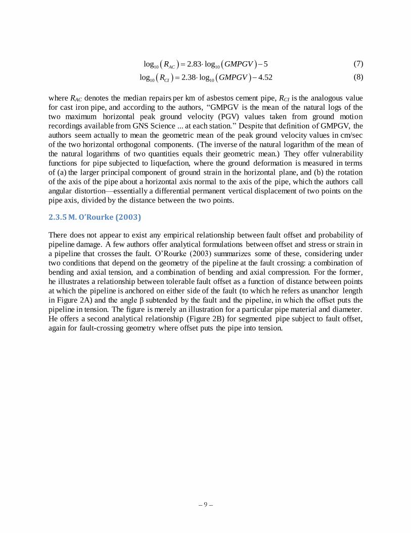
10 10log 2.83 log 5ACR GMPGV (7)
10 10log 2.38 log 4.52CIR GMPGV (8)
where RAC denotes the median repairs per km of asbestos cement pipe, RCI is the analogous value
for cast iron pipe, and according to the authors, “GMPGV is the mean of the natural logs of the
two maximum horizontal peak ground velocity (PGV) values taken from ground motion
recordings available from GNS Science ... at each station.” Despite that definition of GMPGV, the
authors seem actually to mean the geometric mean of the peak ground velocity values in cm/sec
of the two horizontal orthogonal components. (The inverse of the natural logarithm of the mean of
the natural logarithms of two quantities equals their geometric mean.) They offer vulnerability
functions for pipe subjected to liquefaction, where the ground deformation is measured in terms
of (a) the larger principal component of ground strain in the horizontal plane, and (b) the rotation
of the axis of the pipe about a horizontal axis normal to the axis of the pipe, which the authors call
angular distortion—essentially a differential permanent vertical displacement of two points on the
pipe axis, divided by the distance between the two points.
2.3.5 M. O’Rourke (2003)
There does not appear to exist any empirical relationship between fault offset and probability of
pipeline damage. A few authors offer analytical formulations between offset and stress or strain in
a pipeline that crosses the fault. O’Rourke (2003) summarizes some of these, considering under
two conditions that depend on the geometry of the pipeline at the fault crossing: a combination of
bending and axial tension, and a combination of bending and axial compression. For the former,
he illustrates a relationship between tolerable fault offset as a function of distance between points
at which the pipeline is anchored on either side of the fault (to which he refers as unanchor length
in Figure 2A) and the angle β subtended by the fault and the pipeline, in which the offset puts the
pipeline in tension. The figure is merely an illustration for a particular pipe material and diameter.
He offers a second analytical relationship (Figure 2B) for segmented pipe subject to fault offset,
again for fault-crossing geometry where offset puts the pipe into tension.

– 10 –
A
B Figure 2. A. Tolerable fault offset vs. unanchor length in continuous pipe (O'Rourke 2003, citing Kennedy et al., 1977), and
B. Tolerable fault offset versus pipe -fault intersection angle in segmented pipe (O'Rourke 2003, citing O’Rourke and Trautmann, 1981)
2.4 Tasks and methods to repair leaks and breaks
The city of Winnipeg (2014) offers a list of tasks to repair a water main break, written for the
general public. The tasks are shown in chronological order in the left-hand column of Table 2. The
task list is generally consistent with a more detailed checklist created by the American Water
Works Association (2008) although it omits lists of tools, equipment, disinfecting chemicals,
documentation, and testing materials. Column 2 of the table lists my interpretation of rate-limiting
factors, that is, prerequisites for each task. The rate-limiting factors are mostly potential impacts
from other lifelines, that is, lifeline interactions. If they are unavailable, repairs cannot proceed or
they proceed more slowly—that is, their rate is limited. These items include communications,
electricity, fuel, site safety (i.e., no fire or hazardous material release), roadway access, repair
crews, and repair supplies (replacement pipe, replacement fittings, clamps, and paving materials).
Regarding crew availability, public and private water agencies plan to provide mutual assistance
for emergencies; see CalWARN (2008) for example. Crews may have to travel from great
distances, hundreds of miles or more, so their availability can change over time. Table 2 probably
omits tasks that are unnecessary or trivial for day-to-day repairs but become significant in a large

– 11 –
earthquake. For example, a water agency may also have to arrange repair contracts with
contractors, track and prioritize repairs, and manage an unusually large number of repair crews
operating simultaneously.
Table 2. Water pipeline repair tasks
Tasks Rate-limiting factors
1. Receive a notice from our 311 Centre about a water
main break.
Communications, electricity
2. Dispatch a crew to the location. Fuel, site safety (e.g., no fire),
roadway access, crew availability
3. Control the leak to reduce the risk to public safety, and
private and public property. We do this by finding and
closing valves.
4. Contact other utilities to make sure that we can dig
without damaging other services or endangering staff
or the public.
Communications
5. Pinpoint the location of the leak using an electronic
leak detector.
6. Dig down to the water main and confirm the cause of
the leak.
Fuel
7. Repair the water main. Depending on the type of break,
we may apply a repair clamp or replace a length of
pipe.
Pipe, fitting, or repair hardware
such as clamps
8. Open valves to turn the water main back on, flush the
water main and sample water quality.
9. Backfill to temporarily restore the excavated area. Fuel
10. Permanently restore the sod or pavement in the
excavated area.
Pavement material
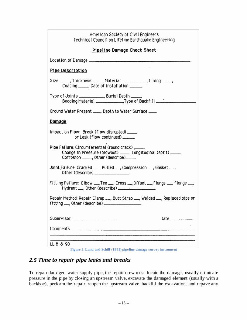
Lund and Schiff (1991) surveyed pipeline utilities, asking them to provide detailed information
about each pipeline failure they repaired after the 1989 Loma Prieta earthquake. See Figure 3 for
the survey instrument. The resulting database includes information about 862 pipeline failures
among 65 water, sewer, drainage, and gas agencies. The data may be useful for estimating repair
times, so I extracted the following statistics from the database.
Burial depth. Among 67 records with reported burial depth, the average was 4.0 feet and
the standard deviation was 2.2 ft.
Break or leak. Among the failures where the respondent indicated whether the failure was
a break or a leak, it was more common for the pipeline to break (336 failures) than to leak
(140 failures).
Pipe failure modes. Among pipe failures, the most common were circumferential cracks
(99), followed by splits (43) and corrosion (33). Only one blowout was reported.
Joint failure modes. Almost as common as pipe failures were joint failures: 102 pulled, 29
cracks at joints, 25 gasket failures, and 12 other joint failures.

– 12 –
Fitting failure modes. There were a variety of fitting failures: 57 threaded couplings, 9
elbows, 6 offsets, 4 hydrants, 3 tees, and 45 miscellaneous other fitting failures.
Repair methods. The most common repair method was to replace the damaged element
(185 replacements), more than twice the number of clamps installed (77), followed by
mechanical couplings (50), epoxy glue (16), and miscellaneous others such as flex
couplings and pressure grout.
– 13 –
Figure 3. Lund and Schiff (1991) pipeline damage survey instrument
2.5 Time to repair pipe leaks and breaks
To repair damaged water supply pipe, the repair crew must locate the damage, usually eliminate
pressure in the pipe by closing an upstream valve, excavate the damaged element (usually with a
backhoe), perform the repair, reopen the upstream valve, backfill the excavation, and repave any

– 14 –
driving surface over the location of the repair. Pipe damage can be repaired by replacing the
damaged element, by welding over the crack, or by installing repair hardware: generally either a
clamp that is mechanically secured over the damage or a closure ring called a butt strap that is
welded to the outside of the pipe over the damage. The time required to perform the repair depends
on several issues:
How long it takes people to report the damage to the utility or otherwise for the utility to become aware of and locate the damage, which itself depends on power and
communication;
Site accessibility;
Availability of crews and equipment;
Availability of fuel and consumable repair material;
Pipe burial depth;
Groundwater presence and depth;
Diameter, material, and jointing of the pipe;
Impact on flow (break or leak);
Nature of the damaged element: whether to pipe, joint, or fitting;
If pipe, whether circumferential crack, longitudinal split, corrosion, etc.;
If joint, whether a crack, pull-out, compression failure, gasket failure, etc.;
If fitting, the nature of the fitting (elbow, tee, cross, offset, etc.);
Schiff (1988) offers repair times for 21 individual water pipe repairs after the 1987 Whittier
Narrows earthquake, mostly of cracks and breaks in 4 to 8-inch steel and cast iron mains. Repair
times were reported by the Whittier water distribution superintendent. Times varied between 1 and
16 hours, as shown in Table 3. Schiff reports that water pressure in Whittier dropped to 50 psi
from the normal 80 to 100 psi as a result of 40 breaks in 133 miles of pipe (or 0.06 breaks per 1000
lf of pipe).

– 15 –
Table 3. Repair times for water supply pipeline damage in the 1987 Whittier Narrows Earthquake (Schiff 1988)
East Bay Municipal Utility District (2014) reports on its mutual assistance to the City of Napa after
the 24 Aug 2014 M 6.0 South Napa earthquake. EBMUD crews performed 56 repairs in
approximately 252 crew-hours, for an average duration of 4.5 hours per repair. It should be noted
that this average duration for completing repairs does not reflect the time it took for the City of
Napa or its contractors to complete the excavation and backfill (EBMUD crews focused on repair
work, and did not complete excavation/backfill/paving-related work).
Tabucchi et al. (2010) elicited opinion from personnel at the Los Angeles Department of Water
and Power on repair productivity. They propose a model with triangular probability distributions
for each of several repair operations. Each distribution is characterized by a minimum value (the
left end of the triangle), a modal value (the peak of the triangle, which is the most likely value),
and a maximum value (the right end of the triangle). Table 4 repeats LADWP’s estimates .

– 16 –
Distribution-system leak and break repairs are estimated to require no less than 3 hours and no
more than 12 hours with modes of 4 to 6 hours.
Table 4. Tabucchi et al. (2010) LADWP repair productivity estimates
Hazus-MH (NIBS and FEMA 2012) employs four restoration times: two each for large and small
diameter pipes (20 inch diameter and above is large, 12 inches or less is small) times two to
distinguish between breaks and leaks. See Table 5.

– 17 –
Table 5. Hazus-MH (2012) estimates of repair time per pipe repair
Seligson et al. (1991) offer an empirical relationship for time required to restore water service as
a function of number of pipeline breaks per square mile, based on evidence from the 1971 San
Fernando and 1987 Whittier earthquakes. In Equation (9), B denotes breaks per square mile and d
denotes number of days of water supply outage:
2.18 2.51 ln 0.42
0 0.42
d B B
B
(9)
2.6 Serviceability of water supply
As previously noted, some analytical models are capable of modeling the serviceability of a
damaged water supply system using hydraulic or connectivity analysis (e.g., Khater and Grigoriu
1989). As in the case of the closely related LLEQE software, the Applied Technology Council
(1991) noted that such systems can be data intensive and computationally demanding. What can
be done to estimate water supply serviceability without a hydraulic model?
Isoyama and Katayama (1982) propose to measure a quantity they call serviceability as the
probability that the demand at a system node (such as a customer service connection) is fully
satisfied, or in the aggregate, the average fraction of nodes in the entire system whose demand is
fully satisfied. Demand seems to mean the pre-earthquake consumption plus post-earthquake
leakage.
Markov et al. (1994) propose to measure serviceability via a serviceability index SS defined as the
ratio of the total available flow to the total required flow, which is similar but not identical to
Isoyama and Katayama’s serviceability. If demand at 10 nodes were fully satisfied and demand at
10 other nodes were partially satisfied, the two measures of serviceability would take on different

– 18 –
values: 0.5 in the case of Isoyama and Katayama (1982) and somewhat higher in the case of
Markov et al. (1992).
The developers of the Hazus-MH water system use data from Isoyama and Katayama (1982) and
Markov et al. (1994), along with unpublished work by G&E Engineering Systems to propose to
estimate the serviceability index s(r) as a function of break rate (breaks, not leaks, per km of service
main pipe) using Equation (10). They seem to use the serviceability index to measure the fraction
of customers receiving any water service, since the software expresses loss of serviceability in
terms of “households without water.”
ln
1r L q
s rb
(10)
In Equation (10), ln denotes natural logarithm, r/L denotes the average break rate (r main breaks
per L km of pipe), q and b are model parameters, and is the standard normal cumulative distribution function (the y-value of the S-shaped curve in x-y space that depicts the probability
that an uncertain quantity with standard normal distribution will take on a value less than or equal
to x). Hazus-MH employs values of q = 0.1 and b = 0.85, respectively, fitting the curve to Isoyama
and Katayama’s modeling of Tokyo’s water supply system, Markov et al.’s modeling of the San
Francisco Auxiliary Water Supply System (a dedicated firefighting system), and G&E’s
unpublished analyses of East Bay Municipal Utility District’s water supply system. Hazus’
serviceability model is illustrated in Figure 4, in the curve labeled “NIBS.”
Figure 4. Hazus-MH model of serviceability. Hazus uses the curve labeled “NIBS.”
Thus, the Hazus-MH serviceability index might measure:

– 19 –
The fraction of service connections receiving pre-earthquake flows, regardless of the degree of post-earthquake flow received at other service connections, which would seem
to be consistent with Isoyama and Katayama’s (1982) serviceability.
The fraction of pre-earthquake flow being delivered after the earthquake, consistent with
Markov et al. (1994); or
The fraction of service connections receiving any water, as the Hazus-MH reports indicate.
Lund et al. (2005), citing Kobe Municipal Waterworks Bureau’s M. Matsushita, present a
restoration curve for the Kobe water system after the 1995 Kobe earthquake. Tabucchi and
Davidson (2008) offer an analogous plot for the restoration of water service in the San Fernando
Valley after the 1994 Northridge earthquake. The two restoration curves are duplicated in Figure
5. Restoration after Northridge appears fairly linear; Kobe less so.
A B Figure 5. A. Restoration of water service after the 1994 Northridge earthquake and B. After the 1995 Kobe earthquake
2.7 Lifeline interaction
Many authors have characterized lifeline interaction after natural disasters. A few but not all
relevant works are summarized here.
For ease of reference, let us recall here some evidence previously noted: Winnipeg (2014) and
AWWA (2008) suggest that prerequisites for the repair of buried pipeline include cellular
communications and electricity to learn about and coordinate repairs, fuel and roadway access to
travel to and perform the repairs, site safety (especially no fires, gas leaks, or electrical hazards),
and consumable repair materials including pipe, fittings, repair hardware, and disinfecting
chemicals.
Nojima and Kameda (1991) compiled instances of lifeline interaction in the 1989 Loma Prieta
earthquake, noting particularly the loss of wastewater treatment because of the loss of electricity,
and the degradation of telecommunications resulting from the loss of electricity and difficulty
acquiring fuel for central offices’ emergency generators as a result of highway problems. See Table
6 for a matrix summarizing lifeline interaction in the earthquake. It shows that water supply was
impaired for 18 hours in Santa Cruz because of loss of electric power for pumping. It also shows
that electricity failure impaired EBMUD’s Lafayette filtration plant and its Oakland Control

– 20 –
Center. Repairs in Santa Cruz were also impaired by delays transporting repair equipment over the
damaged Oakland-San Francisco Bay Bridge. In San Francisco and Santa Cruz, overloaded
telecommunications impaired repair efforts.
Scawthorn (1993) reviews literature and then-recent disaster experience on lifeline interaction in
several disasters (1989 Cajon Pass, 1989 Loma Prieta Earthquake, 1991 Shasta spill, 1991 East
Bay Hills fire, and 1992 Hurricanes Andrew and Iniki) to construct a model and analytical
methodology for lifeline interaction. He points out that water supply in the 1991 Oakland Hills fire
was impaired in part because of breakage of service connections in buildings that collapsed in the
fire, and the reliance of water supply on electric power to pumps stations that were required to
resupply ridge-top tanks. He suggests characterizing lifeline interactions as either: (a) cross-impact
(impact on one lifeline's function due to impairment of service to that lifeline by a second lifeline),
collocation (direct damage or impact on one lifeline's function due to failure of another lifeline in
a very proximate location), and cascade (increasing impacts on a lifeline due to initial
inadequacies, e.g., water supply damage as buildings collapse and sever service connections). In
Scawthorn’s quantitative model, one characterizes initial damage to a set of lifelines through a
vector D of n scalar quantities, each element representing a fraction of customers receiving service
for one of n lifelines if there were no interaction, i.e., if only damage to that lifeline mattered.
Lifeline interaction is quantified by an n x n matrix denoted by L, where element Li,j (row i, column
j) denotes the fraction of service of lifeline i that is contributed by lifeline j. A higher value of Li,j
indicates greater reliance of lifeline i service on lifeline j. A value Lij = 0 indicates no interaction.
The final functional state of the n lifelines is represented by vector F, whose value is given by
Equation (11). Element i of vector F measures the fraction of customers receiving service from
lifeline i, where any reduction below Fi = 1.0 is a result of initial damage D to all the lifelines and
interaction L between them.
F LD (11)
Scawthorn offers the model but does not propose particular values for matrix L. Note that, because
0 ≤ Di ≤ 1.0, to ensure that 0 ≤ Fi ≤ 1.0, L must be constrained per Equation (12).
1
1.0 1, 2,...n
ij
j
L i n
(12)

– 21 –
Table 6. Lifeline interaction matrix in the Loma Prieta earthquake (after Nojima and Kameda 1991)
Electricity Gas Water Sewer Road Rail Telephone
Electricity
*
Santa Cruz gas explosion due to electricity comeback (spark ignition). Recovery work arrangement with electric power supply system
Santa Cruz: pump stopped for 18 hrs (gravity flow area survived; no water in pump-based supply area) SF: power failure due to gas leak inspection, no water in pump-based supply area
and Marina district. No power for repair work. EBMUD: short-term loss of power at Lafayette filtration plant. Oakland Control Center power loss, no service
SF and Santa Cruz: power failure at pump station
SF and Santa Cruz: traffic jam due to malfunction of traffic signal
SF: BART omitted stops at some stations to save electricity
Capacity diminished by use of storage cells. PBX with no battery, malfunction Pacific Bell: Bush/Pine Office (SF) coolant trouble;
no service for 3 hrs. Hollister Office generator failure no service for 3 hrs. GTE: Monte Bello Office (Los Gatos) failure of generator fuel tank;
malfunction (6-7 hrs)
Gas SF & Santa Cruz: gas leak inspection before recovering electricity
*
Santa Cruz: no home treatment. Recovery work arrangement with gas supply system.
SF: road closed due to propane fire (Rte. 80 WB Central Ave)
Water Santa Cruz: recovery work arrangement with water supply system
*
Santa Cruz: damage detection by analogy
SF Marina District: road failure due to water leakage
Sewer Santa Cruz: suspicion of underground water
contamination due to outflow or crude sewage from pipeline
*
Road Santa Cruz: no transporting machinery due to bridge damage
Santa Cruz: damage detection by analogy
*
BART riders increased due to Bay Br. Closure (Oct 23: +40 percent)
Rail *
Telephone SF & Santa Cruz: overload *

– 22 –
The San Francisco Lifelines Council (2014) adapted the panel process of Porter and Sherrill (2011)
to involve Bay Area lifeline operators in qualitatively characterizing the potential effects of lifeline
interaction on the post-earthquake functionality of their systems. The authors sought to identify
key assets and restoration schemes to prioritize post-disaster restoration and reconstruction
activities for San Francisco and ultimately the Bay Area. Through panel discussion with 11 lifeline
operators, the authors identified lifeline interaction effects in the context of a hypothetical M 7.9
earthquake on the Northern San Andreas Fault. They propose a qualitative interaction matrix
(Table 7) that describes modes of interaction a la Nojima and Kameda (1991) and shows a degree
of interaction, with darker shading indicating greater interaction, like a higher value in Scawthorn’s
(1993) matrix. The authors found that restoring water supply in San Francisco depends
significantly on city streets, telecom, and fuel, and to a lesser extent on regional roads, electric
power, and the port. The matrix characterizes the mode of each interaction, with five possible
modes. Quotations are taken from San Francisco Lifelines Council (2014); interpretations are
mine:
“Functional disaster propagation and cascading interactions from one system to another due to interdependence.” This means that a system relies on one or more other systems to
operate, each of which can rely on still others. Let us refer to these other systems as
“upstream,” in the sense that failure of an upstream system flows or cascades down to the
system in question and causes its failure. For example, consider water service in a pressure
zone that is supplied from tanks whose source is water pumped from lower elevation. Water
service in that pressure zone is functionally dependent on electricity, which may be
functionally dependent on natural gas. Failure of fuel supplies or electric generation,
transmission, or distribution propagates or cascades to cause water supply failure through
interdependence.
“Collocation interaction, meaning physical disaster propagation among lifeline systems .”
This means that one or more elements of the system in question are located close to one or
more elements of another system, and that the other system can fail in such a way that an
area around the failure can impair the system in question. For example, fiber optic cable
that serves the telecommunication network may be installed in a conduit on a roadway
bridge. Excessive displacement of the bridge, for example as a result of settlement of an
abutment, can sever the fiber conduit.
“Restoration interaction, meaning various hindrances in the restoration and recovery stages.” This means that one or more elements of the system in question are located close
to one or more elements of another system, and that repairs to the other system can damage
or hinder the repair of the system in question. For example, consider a water main (the
system in question) that is located above a damaged sewer line. Repair to the sewer line
could require the temporary removal of or inadvertently lead to damage to the water main.
“Substitute interaction, meaning one system’s disruption influences dependencies on
alternative systems.” This means that the system in question may have substitutes
(alternative systems), and that disruption of one of the alternatives can affect the system in
question. For example, damage to the San Francisco-Oakland Bay Bridge in the 1989 Mw

– 23 –
6.9 Loma Prieta earthquake caused a 32% increase in BART ridership during October and
November 1989 (San Francisco Bay Area Rapid Transit District 2015).
“General interaction, meaning between components of the same system.” Nojima and Kameda (1991) use a star (*) to mean the same thing. This means that impairment of
elements of the system in question can affect other elements of the same system. For
example, overturning of electrical switchgear in a pumping station can cause the pumps to
fail to operate.

– 24 –
Table 7. The San Francisco Lifelines Council’s (2014) lifeline system interdependencies matrix

– 25 –
2.8 Pipeline damage in afterslip
Several authors have considered lifeline damage due to afterslip, which is fault slip immediately
following an earthquake rupture that involves creep much faster than the interseismic rate.
According to Aagaard et al. (2012), “Afterslip develops very quickly and can have similar impacts
as coseismic slip, with the added complexity that the slip continues for months to years, albeit with
a decreasing rate.” They discuss afterslip in various Hayward Fault earthquake scenarios, including
the one adopted for use here: “Afterslip makes a substantial contribution to the long-term geologic
slip and may be responsible for up to 0.5–1.5 m (median plus one standard deviation) of additional
slip following an earthquake rupture.” The authors offer a power-law expression for afterslip as a
function of time t, denoted D(t), as follows:
1
1C
D t A BT t
(13)
1
1total coseismicA D a D
a
(14)
1
total coseismic
aB D D
a
(15)
11sec
CT
a
(16)
0.881 0.111median wC M (17)
where T is referred to as the afterslip time constant, taken here as 365 days per Aagaard et al.
(2012). For example, with Mw = 7.05, Equation (17) leads to Cmedian = 0.0984. With T = 365 days,
Equation (16) leads to a = 5.47. With Dtotal = 1.86m and Dcoseismic = 0.83m, Equations (13), (14),
and (15) produce A = 0.608m, B = 1.25m, and the estimate of slip versus time shown in Figure 6.
Figure 6. Illustration of afterslip
O’Rourke and Palmer (1996) point out that understanding observations of pipeline damage at fault
crossings requires estimating fault slip from the time of pipeline installation to the time of its
0.0
0.5
1.0
1.5
2.0
0.00001 0.001 0.1 10 1000
Sli
p, m
Time after mainshock, days

– 26 –
excavation for inspection after the earthquake, including pre-seismic slip, coseismic slip, and
afterslip.
Treiman and Ponti (2011) suggested that afterslip could realistically account for 40% of the total
surface slip in the Coachella Valley resulting from a M 7.8 earthquake on the Southern San
Andreas Fault. The afterslip could aggravate damage to the Coachella Canal, railroad, fiber optic
cable, electrical lines, gas and oil pipelines, and highways.
Hudnut et al. (2014) measured deformation in a temporarily decommissioned 26-inch diameter
gas pipeline that crosses the fault rupture involved in the 2014 South Napa earthquake. They
observed that the pipeline was “subtly warped more than 35 cm by fault offset, most of which
accumulated as afterslip that is still continuing as of 3 months after the earthquake.” They argue
that “Lifeline performance in future events, with both coseismic slip and afterslip, deserves
additional consideration.”
2.9 Measuring loss of resilience
Bruneau et al. (2003) propose to measure the loss of resilience as the area above the curve Q(t),
where Q(t) is defined (somewhat vaguely) as the “quality of the infrastructure of a community”
They denote a quantity they call “community earthquake loss of resilience” by R and calculate it
as in Equation (18):
1
0
1
t
R Q t dt (18)
where t = 0 and t = t1 denote the times of the initiating event and the time of full restoration,
respectively. For brevity, let us refer to R more simply as the loss of resilience. Bruneau et al. do
not define t = 0 and t = t1 precisely. Let us define t = 0 here as the time of the first earthquake in
the earthquake sequence under consideration, and let us define t1 as the time when Q(t) = 1 after
the last earthquake in the sequence under consideration. Let Q(t) measure the fraction of water
customers receiving at least an adequate degree of service at time t, meaning sufficient water flow
and pressure at the tap for drinking (even if it needs to be boiled first), bathing, and using toilets.
R has units of time, and as applied here can be seen here as the expected value of the time that an
arbitrary customer is receives less water than a useful degree of service.
To be clear, a reduction in the loss of resilience indicates a briefer average time that an arbitrary
customer lacks adequate service, but I will not equate a reduction in the loss of resilience with an
increase in resilience. In Bruneau et al.’s terminology, resilience is not a quantity but rather a
quality that means “the ability of the system to reduce the chances of a shock, to absorb a shock if
it occurs (abrupt reduction of performance) and to recover quickly after a shock (re-establish
normal performance).” Resilience is not the mathematical complement of the loss of resilience.
3. Methodology
3.1 Overview of the methodology

– 27 –
Using the brief literature review of section 2 as a basis, I propose the following methodology. A
lifeline earthquake performance and restoration model typically involves the following analytical
elements:
1. Asset definition, in which the system is described in terms of nodes and links. Nodes have a
location, flow capacity, sometime a value (e.g., replacement cost), and an asset category that
associates the component with one or more relationships between environmental excitation
(e.g., severity of shaking) and loss (e.g., in terms of dollars, deaths, downtime, or some
combination). Links connect nodes. They have a path, sometime a direction, flow capacity,
sometimes a value, and an asset category. The assets in question here are defined in section 4
of this report.
2. Hazard model, relating geographic location to environmental excitation. In the case of
earthquake hazard, the hazard model typically includes a mathematical idealization of seismic
sources in the region, their locations, the frequency with which they can produce earthquakes
of various magnitudes, and one or more ground motion prediction equations to relate
earthquake magnitude and location to shaking and other site effects. In the present study, the
hazard model is presented elsewhere. Briefly, it is a physics-based model of the San Francisco
Bay Area, depicted in Aagaard et al. (2010a, b).
3. Hazard analysis, in which one evaluates the hazard model for one or more realizations of an
earthquake. In the present analysis, I use the realization from Aagaard et al. (2010) depicting
a Mw 7.05 rupture of the Hayward Fault north and south segments with an epicenter under
Oakland. Accompanying the model of shaking from the mainshock are estimates of
liquefaction probability, landslide probability, coseismic slip, and afterslip associated with the
mainshock, along with shaking in each of a sequence of 16 aftershocks of M 5.0 and greater.
4. Vulnerability model, relating environmental excitation at a particular location to the potentially
uncertain loss in each of a set of asset classes. Section 3.2 presents the vulnerability model
used here.
5. Damage analysis, in which one evaluates the vulnerability model for each lifeline component
at the level of environmental excitation to which the component is subjected. Section 3.3
presents the procedures of the damage analysis.
6. Restoration model, which characterizes the time to restore the damaged components to their
pre-disaster condition, and calculates the degree of service at each of many points in time.
Section 3.4 presents the restoration model developed and employed here. The present
restoration model is new. It includes a new method for quantifying the effects of lifeline
interaction. It includes an initial assessment period suggested by engineers of the East Bay
Municipal Utility District, along with a period during which repair crews and other resources
ramp up from an initial, in-house quantity to one that includes mutual aid.
7. Aftershock analysis, in which one inserts one or more aftershocks into the restoration process,
which in a sense restarts the hazard, damage, and restoration analyses with a still -damaged
lifeline system.
3.2 Vulnerability model
3.2.1 What is a vulnerability model?
By “vulnerability model” is meant a mathematical formulation of the relationship between loss
(usually normalized by quantity, e.g., pipeline breaks per 1,000 ft of pipe) and environmental

– 28 –
excitation (e.g., degree of peak ground velocity). These relationships often apply to classes of
components that share common engineering features, e.g., pipe sharing common material,
diameter range, joint type, etc. All specimens of the class are assumed to be interchangeable and
indistinguishable for purposes of estimating loss. A vulnerability model can be deterministic,
providing for example only a mean estimate of loss conditioned on excitation, or probabilistic,
providing both a mean value and error term. Let us define some terms:
yi(x) = the expected value of the degree of loss experienced by a component of class i when
subjected to excitation x. One can refer to yi(x) as the mean vulnerability function for class
i.
i(x) = the error term for class i. The error term can be constant for class i or it can depend on degree of excitation x. The error term has unit mean and usually has some parametric
distribution, such as lognormal with a specified standard deviation of the natural logarithm
of the error term, referred to here as the logarithmic standard deviation. The vulnerability
model can provide mean vulnerability functions and error terms for one or more modes of
damage j, such as damage by wave passage and damage by ground failure due to
liquefaction, landslide, or fault offset.
yi,j(xi,j) = the mean loss to a component i of a specified class in damage mode j when component i
is subjected to mode-j excitation xi,j, such as the peak ground velocity to which a particular
segment of pipe is subjected.
i,j(xi,j) = the mode-j vulnerability error term for the class to which component i belongs, when the
component is subjected to excitation xi,j.
Yi,j(xi,j) = the uncertain normalized loss is denoted by (e.g., uncertain total pipeline breaks per 1,000
lf of pipe), where the index i refers to the component class to which component i belongs,
j refers to the damage mode under consideration (e.g., pipeline breaks per 1,000 lf of pipe
as a result of wave passage), and xi,j is as previously defined.
The uncertain normalized loss is calculated as:
, , , , , ,i j i j i j i j i j i jY x y x x (19)
The vulnerability model comprises the set of functions y and , the component classes to which they refer, and the domain of excitations for which the functions are valid.
3.2.2 Selecting a vulnerability model for a pipeline network
Several authors have created and published pipeline vulnerability functions; a few appear in
section 2. There are no commonly accepted rating systems for pipeline vulnerability functions, but
it seems reasonable to choose among competing vulnerability functions based on at least the
following criteria:
Vulnerability functions reflect diverse conditions: pipe material, diameters, joint systems, age, and corrosivity similar to the conditions where the vulnerability functions will be
applied.
Vulnerability functions are drawn from numerous damage data.
Vulnerability functions are drawn from ground motion levels reaching as high as those
where they will be applied.
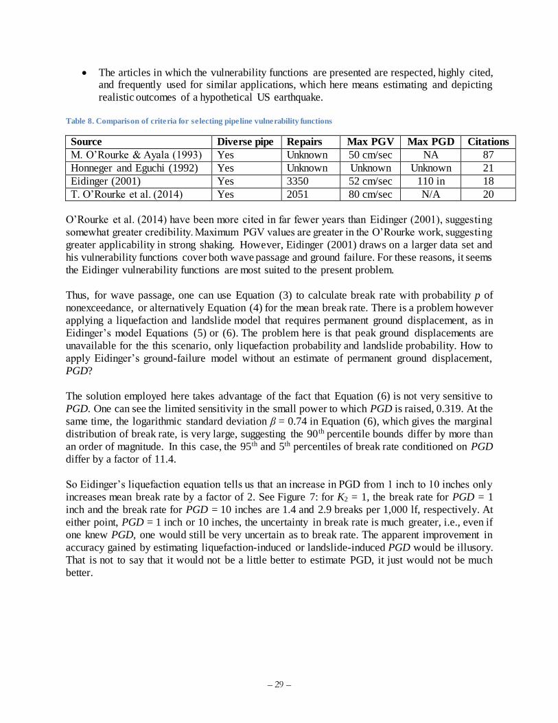
– 29 –
The articles in which the vulnerability functions are presented are respected, highly cited, and frequently used for similar applications, which here means estimating and depicting
realistic outcomes of a hypothetical US earthquake.
Table 8. Comparison of criteria for selecting pipeline vulnerability functions
Source Diverse pipe Repairs Max PGV Max PGD Citations
M. O’Rourke & Ayala (1993) Yes Unknown 50 cm/sec NA 87
Honneger and Eguchi (1992) Yes Unknown Unknown Unknown 21
Eidinger (2001) Yes 3350 52 cm/sec 110 in 18
T. O’Rourke et al. (2014) Yes 2051 80 cm/sec N/A 20
O’Rourke et al. (2014) have been more cited in far fewer years than Eidinger (2001), suggesting
somewhat greater credibility. Maximum PGV values are greater in the O’Rourke work, suggesting
greater applicability in strong shaking. However, Eidinger (2001) draws on a larger data set and
his vulnerability functions cover both wave passage and ground failure. For these reasons, it seems
the Eidinger vulnerability functions are most suited to the present problem.
Thus, for wave passage, one can use Equation (3) to calculate break rate with probability p of
nonexceedance, or alternatively Equation (4) for the mean break rate. There is a problem however
applying a liquefaction and landslide model that requires permanent ground displacement, as in
Eidinger’s model Equations (5) or (6). The problem here is that peak ground displacements are
unavailable for the this scenario, only liquefaction probability and landslide probability. How to
apply Eidinger’s ground-failure model without an estimate of permanent ground displacement,
PGD?
The solution employed here takes advantage of the fact that Equation (6) is not very sensitive to
PGD. One can see the limited sensitivity in the small power to which PGD is raised, 0.319. At the
same time, the logarithmic standard deviation β = 0.74 in Equation (6), which gives the marginal
distribution of break rate, is very large, suggesting the 90th percentile bounds differ by more than
an order of magnitude. In this case, the 95th and 5th percentiles of break rate conditioned on PGD
differ by a factor of 11.4.
So Eidinger’s liquefaction equation tells us that an increase in PGD from 1 inch to 10 inches only
increases mean break rate by a factor of 2. See Figure 7: for K2 = 1, the break rate for PGD = 1
inch and the break rate for PGD = 10 inches are 1.4 and 2.9 breaks per 1,000 lf, respectively. At
either point, PGD = 1 inch or 10 inches, the uncertainty in break rate is much greater, i.e., even if
one knew PGD, one would still be very uncertain as to break rate. The apparent improvement in
accuracy gained by estimating liquefaction-induced or landslide-induced PGD would be illusory.
That is not to say that it would not be a little better to estimate PGD, it just would not be much
better.

– 30 –
Figure 7. Eidinger (2001) pipe liquefaction vulnerability for K2 = 1.0, mean and 90% bounds
In light of the very high uncertainty in break rate and the relatively modest sensitivity of the
vulnerability function to PGD, let us assume a reasonable moderate PGD associated with
liquefaction, say 6 inches, and rewrite Equations(5) and (6) using liquefaction probability, as
shown in Equations (21):
0.319 1
2
1
2
, 1.06 6 exp 0.74
1.88 exp 0.74
l L L
L
R P p K P p
K P p
(20)
0.319
2
2
1.39
2.46
l L L
L
R P K P
K P
(21)
where PL denotes probability of ground failure, either through liquefaction, landslide, or fault
offset. The equation estimates mean break rate per 1,000 linear feet of pipe.
How does one sum break rates from wave passage and ground failure if one uses Eidinger’s (2001)
model? He says that “wave propagation effects are masked within the more destructive effects of
[peak ground displacements].” If one knew where ground failure occurs, one would ignore the
wave-passage model so as not to double-count it. The problem here is that Eidinger’s empirical
model of damage due to liquefaction probably includes some damage that was caused by wave
passage. But he does not know which breaks were caused by which peril. In zones of liquefaction,
he treats all damage as caused by liquefaction. That is, his empirical relationship for damage in
zones of liquefaction include an unknown (but probably small) fraction of damage caused by wave
passage.
0.0
2.5
5.0
7.5
10.0
0 5 10 15 20
Bre
ak
s p
er 1
000 l
f p
ipe
Permanent ground deformation, in.
R(0.95)
R(0.05)
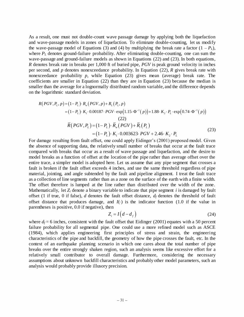
– 31 –
As a result, one must not double-count wave passage damage by applying both the liquefaction
and wave-passage models in zones of liquefaction. To eliminate double-counting, let us modify
the wave-passage model of Equations (3) and (4) by multiplying the break rate a factor (1 – PL),
where PL denotes ground-failure probability. After eliminating double-counting, one can sum the
wave-passage and ground-failure models as shown in Equations (22) and (23). In both equations,
R denotes break rate in breaks per 1,000 ft of buried pipe, PGV is peak ground velocity in inches
per second, and p denotes nonexceedance probability. In Equation (22), R gives break rate with
nonexceedance probability p, while Equation (23) gives mean (average) break rate. The
coefficients are smaller in Equation (22) than they are in Equation (23) because the median is
smaller than the average for a lognormally distributed random variable, and the difference depends
on the logarithmic standard deviation.
1 1
1 2
, , 1 , ,
1 0.00187 exp 1.15 1.88 exp 0.74
L L w L L
L L
R PGV P p P R PGV p R P p
P K PGV p K P p
(22)
1 2
, 1
1 0.003623 2.46
L L w l L
L L
R PGV P P R PGV R P
P K PGV K P
(23)
For damage resulting from fault offset, one could apply Eidinger’s (2001) proposed model. Given
the absence of supporting data, the relatively small number of breaks that occur at the fault trace
compared with breaks that occur as a result of wave passage and liquefaction, and the desire to
model breaks as a function of offset at the location of the pipe rather than average offset over the
entire trace, a simpler model is adopted here. Let us assume that any pipe segment that crosses a
fault is broken if the fault offset exceeds 4 inches, and use the same threshold regardless of pipe
material, jointing, and angle subtended by the fault and pipeline alignment. I treat the fault trace
as a collection of line segments rather than as a zone on the surface of the earth with a finite width.
The offset therefore is lumped at the line rather than distributed over the width of the zone.
Mathematically, let Zi denote a binary variable to indicate that pipe segment i is damaged by fault
offset (1 if true, 0 if false), d denotes the fault offset distance, df denotes the threshold of fault
offset distance that produces damage, and I() is the indicator function (1.0 if the value in parentheses is positive, 0.0 if negative), then
i fZ I d d (24)
where df = 6 inches, consistent with the fault offset that Eidinger (2001) equates with a 50 percent
failure probability for all segmental pipe. One could use a more refined model such as ASCE
(1984), which applies engineering first principles of stress and strain, the engineering
characteristics of the pipe and backfill, the geometry of how the pipe crosses the fault, etc. In the
context of an earthquake planning scenario in which one cares about the total number of pipe
breaks over the entire strongly shaken region, such an analysis seems like excessive effort for a
relatively small contributor to overall damage. Furthermore, considering the necessary
assumptions about unknown backfill characteristics and probably other model parameters, such an
analysis would probably provide illusory precision.

– 32 –
3.3 Damage analysis (number of repairs required)
3.3.1 What is a damage analysis?
A damage analysis applies the vulnerability model and the hazard model to the assets under
consideration to estimate degree of damage or loss, e.g., total number of pipeline repairs required
when a particular pipeline network is affected by a particular earthquake. Let us employ a common
general formulation for number of repairs required for a system of ni discrete components (e.g.,
segments of pipe) that can each be uniquely identified with a class of components (e.g., type of
pipe).
Each component i has an associated quantity or value Vi (e.g., length of pipeline segment), and is
assumed to be subject to damage from up to nj modes of damage (e.g., wave passage and
liquefaction). Each combination of component class and mode of damage is assigned a
vulnerability model yi,j(xi,j) andi,j(xi,j) as previously defined. Let R denote the total uncertain loss
(e.g., total number of pipeline breaks). It is estimated as shown in Equation (25).
, , , ,
jinn
i i j i j i j i j
i j
R V y x x (25)
Equation (25) assumes that damage to one component or in one model is independent of damage
to other components or in other modes. That is, that the degree of damage to component i in mode
j is unaffected by damage to a different component, and that if component i is damaged in one
mode, it can also be damaged in another mode and that the losses resulting from the two modes of
damage simply sum.
In the case of water supply pipelines, one implication of this assumption of independence is that it
assumes that repairs are spaced widely enough apart that it makes sense to repair individual breaks
or leaks, at least initially, rather than to remove and replace pipe and thus repair two or more breaks
with a single repair.
3.3.2 Applying the damage analysis to a water supply system
Applying Equation (25) to water supply pipelines using Eidinger’s (2001) vulnerability model,
and adding an additional term for fault crossings, one can estimate mean total number of repairs r
as shown in Equation (26):
,
1 1 1
, 1, 2, ,
1 1 1
1 0.003623 2.46
n n n
w i i l L i i f
i i i
n n n
L i i i i i L i i f
i i i
r R PGV L R P L I d d
P K PGV L K P L I d d
(26)
where i is an index to pipe segments, n is the total number of segments in the network, K1,i and K2,i
denote the values of K1 and K2 for pipe segment i, PGVi is the peak ground velocity to which
segment i is subjected, PL,i denotes the ground-failure probability at pipe segment i, Li is the length
of pipe segment i in thousands of linear feet, I() is an indicator function that takes on the value 1.0
if the expression in parentheses is positive, 0.0 if negative, di is the fault offset to which a segment of pipe i is subjected, and df is the offset at which breakage occurs. Here I propose to take df as

– 33 –
deterministically equal to 6 inches (15 cm). Note that as long as pipe segments i are relatively
short, less than a few hundred meters, there should be little difference between shaking at the ends,
and thus little error introduced by discretizing a pipeline network in this way.
Because the present analysis does not require a probabilistic estimate of loss, let us ignore the error
term and deal only with the expected value of loss. I use the lower-case r in Equation (26) to indicate a deterministic value rather than the upper-case R of Equation (25) that stands for an
uncertain quantity.
To carry out Equation (26), one uses a geographic information to create a table of system
components, e.g., a table of pipe segments. Components are listed in rows. For each component,
assign an identifier, determine its quantity (e.g., its length), assign it to a class that has one or more
vulnerability or fragility functions (e.g., Eidinger’s classes that group water supply pipe by
material, joint, soil corrosivity, and diameter), and determine its location, e.g., the latitude and
longitude of a pipe segment midpoint. Then using the GIS, look up the ground-motion parameter
values xi,j. Equation (26) can then be calculated for each component (each row) and the losses
summed over all rows to calculate the expected value of loss r (e.g., the number of pipeline breaks
requiring repairs).
3.3.3 Breaks or leaks?
Lund and Schiff (1991) define leaks and breaks for purposes of compiling damage data. Under
their definition, a pipe with a leak continues to function with minimal loss of service while a pipe
with a break completely loses function. It seems as if another, equivalent definition is that a pipe
break separates a pipe segment into two, and a leak only partially fractures a pipe. Hazus-MH
assumes an 80%/20% break/leak ratio for liquefaction, 20%/80% breaks/leaks for wave-passage
damage. The authors of the technical manual do not cite a source for their choices.
Lund and Schiff (1991) found that, among all pipeline failures in the 1989 Loma Prieta earthquake
where it was known whether the failure was a break or a leak, it was more common for the pipeline
to break (336 repairs, 71%) than to leak (140 repairs, 29%). A study by Ballantyne et al. (1990) of
pipe damage in 1949 and 1969 Seattle, 1969 Santa Rosa, 1971 San Fernando Valley, 1983
Coalinga, and 1987 Whittier Narrows earthquakes, found that ground failure resulted in a
50%/50% break/leak ratio, and absent ground failure, the ratio was 15%/85% breaks vs leaks.
Since the present model allows one to distinguish between repairs associated with ground failure
versus wave passage, and since the Ballantyne et al. (1990) are highly regarded and offer their
evidence, I employ their ratios.
3.3.4 Degraded vulnerability?
The model presented here applies the same vulnerability functions to the same system map in the
aftershocks that it applies to the mainshock. Is it correct to do so? Perhaps we should consider a
system that has already been degraded by the mainshock or a large aftershock to be weaker.
Perhaps the mainshock causes small undetected leaks or incipient breaks that become large leaks
or breaks in an aftershock. But there does not seem to be sufficient research available to support
explicitly modeling system degradation—making the mathematical model of the system more
vulnerable in aftershocks than before the mainshock. This is a topic deserving of future research.

– 34 –
3.4 Restoration model
3.4.1 What is a lifeline restoration model?
As used here, a restoration model relates the damage (the output of the damage model) to the
system’s functionality over time, usually depicting its returns to its pre-disaster condition.
Functionality can be measured a variety of ways, but in the case of a utility such as a pipeline
network, it is common to measure functionality in terms of the number of service connections that
receive the lifeline service as a function of time. I do not offer a general mathematical formulation
of a lifeline restoration model, but merely list its elements here, and then propose a particular
solution for the water supply pipeline system examined here. A lifeline restoration model includes
the following elements:
A model of the level of functionality immediately after the disaster
A model of the repair resources—crews and supplies—available over time.
A model of the number of services restored by each repair
A model of the elapsed time after each repair
Ideally, a model of lifeline interaction, i.e., accounting for how damage or restoration of
other lifelines affects or delays damage or restoration of the lifeline in question.
3.4.2 Number of services lost because of earthquake
A hydraulic or connectivity analysis a la Khater and Grigoriu (1989) or Applied Technology
Council (1991) is too demanding for present purposes. Let us use the same simplification as Hazus -
MH does. As noted in the section on serviceability of water supply, Hazus interprets the
serviceability index, which measures the drop in water pressure as a function of the average
number of breaks per km of pipe, as a proxy for the fraction of customers receiving service. Let us
employ the serviceability index the same way: immediately after an earthquake, when the number
of repairs required is r, L is the number of km of pipe in the system, and M is the total number of
customers, then the number of services available immediately after the earthquake is given by M
times the serviceability index of Equation (10). Let V0 denote the number of services available
after the earthquake and before repairs begin:
0
ln
1
V M s r
r
L qM
b
(27)
where M is the total number of services, r is the number of main breaks (not leaks), L is the length
of pipe in the distribution system (km), q = 0.1, and b = 0.85. The parameter q determines the
number of breaks per km (0.1) at which V0 reaches 0.5M. The parameter b determines the width
of the S-shaped curve in Figure 4. How long does it take to complete n repairs?
3.4.3 Number of services restored by the nth repair
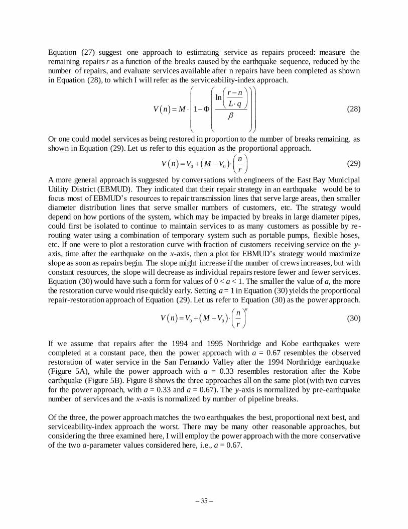
– 35 –
Equation (27) suggest one approach to estimating service as repairs proceed: measure the
remaining repairs r as a function of the breaks caused by the earthquake sequence, reduced by the
number of repairs, and evaluate services available after n repairs have been completed as shown
in Equation (28), to which I will refer as the serviceability-index approach.
ln
1
r n
L qV n M
(28)
Or one could model services as being restored in proportion to the number of breaks remaining, as
shown in Equation (29). Let us refer to this equation as the proportional approach.
0 0
nV n V M V
r
(29)
A more general approach is suggested by conversations with engineers of the East Bay Municipal
Utility District (EBMUD). They indicated that their repair strategy in an earthquake would be to
focus most of EBMUD’s resources to repair transmission lines that serve large areas, then smaller
diameter distribution lines that serve smaller numbers of customers, etc. The strategy would
depend on how portions of the system, which may be impacted by breaks in large diameter pipes,
could first be isolated to continue to maintain services to as many customers as possible by re-
routing water using a combination of temporary system such as portable pumps, flexible hoses,
etc. If one were to plot a restoration curve with fraction of customers receiving service on the y-
axis, time after the earthquake on the x-axis, then a plot for EBMUD’s strategy would maximize
slope as soon as repairs begin. The slope might increase if the number of crews increases, but with
constant resources, the slope will decrease as individual repairs restore fewer and fewer services.
Equation (30) would have such a form for values of 0 < a < 1. The smaller the value of a, the more
the restoration curve would rise quickly early. Setting a = 1 in Equation (30) yields the proportional
repair-restoration approach of Equation (29). Let us refer to Equation (30) as the power approach.
0 0
an
V n V M Vr
(30)
If we assume that repairs after the 1994 and 1995 Northridge and Kobe earthquakes were
completed at a constant pace, then the power approach with a = 0.67 resembles the observed
restoration of water service in the San Fernando Valley after the 1994 Northridge earthquake
(Figure 5A), while the power approach with a = 0.33 resembles restoration after the Kobe
earthquake (Figure 5B). Figure 8 shows the three approaches all on the same plot (with two curves
for the power approach, with a = 0.33 and a = 0.67). The y-axis is normalized by pre-earthquake
number of services and the x-axis is normalized by number of pipeline breaks.
Of the three, the power approach matches the two earthquakes the best, proportional next best, and
serviceability-index approach the worst. There may be many other reasonable approaches, but
considering the three examined here, I will employ the power approach with the more conservative
of the two a-parameter values considered here, i.e., a = 0.67.

– 36 –
Figure 8. Parametric restoration curves with Kobe and Northridge experience
3.4.4 Repair resources and repair rate with lifeline interaction
Now that we can estimate the number of services available after completing n repairs, let us
consider how long it takes to perform n repairs.
Section 2.5 summarizes a few sources of pipe repair time information: an empirical model of per-
break repair time, an empirical model of regional repair time as a function of regional break rate,
and expert opinion of per-break repair time that generally agrees with the empirical evidence, albeit
slightly lower both in terms of lower mean repair time and narrower confidence bounds. Loss
estimation practitioners generally prefer empirical models with explanatory power; for this reason
I employ Schiff’s (1988) pipeline repair data.
I analyzed the (relatively small) sample and found an average repair time of 7.6 hours and a
standard deviation of 5.3 hours. Staff of the San Jose Water Company found that figure to be
reasonable (J. Walsh, oral commun., 14 Oct 2015). A lognormal distribution with median repair
time of 6.5 hours and logarithmic standard deviation of 0.70 fits the data sufficiently well to satisfy
the Lilliefors (1967) goodness of fit test, as shown in Figure 9A. Separating the data for the small-
diameter pipe repairs from the data for two large-diameter pipe repairs (24-inch damage instances,
requiring 12 and 20 hours, respectively), the small-diameter median and logarithmic standard
deviation are 6.1 hours and 0.58, respectively, as illustrated in Figure 9B. Schiff offers too few
samples of large-diameter pipe repair time to derive an empirical distribution, so let us assume a
median of 16 hours and a logarithmic standard deviation of 0.6.
The LADWP estimates of repair duration for distribution pipelines (Tabuchhi et al. 2010)
generally agree with actual earthquake experience reported by Schiff. However they seem to
underestimate uncertainty, with lower and upper limits that include only 70 percent of the repairs
Northridge

– 37 –
reported by Schiff, omitting the lower and upper 15 percent of repair times of Figure 9A. They are
also slightly optimistic, with modes at the 20th and 40th percentiles of repair times in Figure 9A.
It is difficult to compare the Hazus repair times with Schiff (1988) or Tabucchi et al. (2010)
because the former measures repair time per worker and the latter two measure repair time per
repair. However, assuming a crew size of 4, Hazus’ per-worker repair times equate with 6 to 18
hours, or the 35th and 90h percentiles of Figure 9A.
A B Figure 9. Repair times based on data from Schiff (1988): (A) all repairs (B) excluding repairs to large diameter pipe
For a deterministic model, it seems reasonable to use the mean estimate (7.6 hours per repair per
crew, or 0.32 days per repair per crew) for small-diameter pipe repairs (here, assuming crews work
12 hours on, 12 hours off, until repairs are completed.
When will crews become available? As discussed earlier, public and private water agencies plan
to provide mutual assistance for emergencies. CalWARN (ND) and East Bay Municipal Utility
District (2014) report how three Bay Area water agencies dispatched teams to assist in the repair
of water supply pipelines in the City of Napa after the 2014 South Napa earthquake. The assistance
took 24 hours to arrive, which suggests a delay in the arrival of mutual aid from across a
metropolitan region. Mutual aid in a major metropolitan earthquake would likely come from
hundreds, possibly thousands of miles away, and probably take longer to mobilize, arrive, house,
and integrate into repair operations. Repair resources ramp up over time, and the larger the disaster,
probably the longer the ramp-up time. It may take several days to first assess the extent of damage
and locate leaks before actual repairs can be initiated. Let us parameterize this assessment time
and time to ramp up crews using a time-dependent model of the number of repair crews available
to an agency.
c(t) = number of repair crews operating on the day of time t
w(t) = crew workload, fraction of day that crews work, e.g., 0.5 for 12 hours on and 12 hours off
d0 = unconstrained repair duration, days per repair for one crew under ideal conditions, i.e., without
constraints on materials, coordination, and other prerequisites
= 0.32 days on average
0.00
0.25
0.50
0.75
1.00
0 5 10 15 20
Cu
mu
lati
ve
pro
bab
ilit
y
Repair time, hr
0.00
0.25
0.50
0.75
1.00
0 5 10 15 20
Cu
mu
lati
ve
pro
bab
ilit
y
Repair time, hr

– 38 –
i = an index of rate-limiting factors. In Table 2, there are six such factors: communications,
electricity, fuel, site safety (i.e., no fire), roadway access, and repair supplies.
t0 = time at which the 1st repair is performed
t = time at which the nth repair is performed
gi(t) = flow of rate-limiting factor i at time t, normalized so that gi(t) = 1.0 indicates unlimited
availability, gi(t) = 0.5 indicates that the flow or supply rate of factor i is half of what is
normally available, and gi(t) = 0 indicates that factor i is unavailable at time t. If for
example there is no limit on fuel, g of fuel is 1.0. If a utility could only fuel half its repair
vehicles, its g-value would be 0.5. If completing a phone call to coordinate repairs took
twice as long as normal because of communications network congestion, its g-value would
be 0.5. If one could not complete a phone call at all, the g-value for communications would
be 0. In the case of a rate-limiting factor that is a lifeline with a number of service
connections Mi and a number of service connections available at time t denoted by Vi(t),
then
i
i
i
V tg t
M (31)
ui = rate-limiting factor, a constant to indicate the reduction in repair productivity in the absence
of a resources required to perform a repair, also called a u-factor, and indexed by i. One
assigns u-factors based on an estimate of the additional time required to carry out one repair
if it is necessary to do so without the required resource. It is estimated as
01impaired
du
d (32)
Where d0 is the average time required to perform a repair under normal conditions and
dimpaired is the average time it takes to perform a repair when the required resource required
is unavailable. For example, if a repair takes 8 hours normally, but it takes 9 hours in the
absence of a required resource, one assigns u = 1 – 8 hr/9 hr = 0.11. That is, productivity
drops by 11% in the absence of the required resource. Thus, ui = 1.0 indicates that resource
i is critical to repairs: without it, repairs do not proceed. A u-value of 0.5 indicates that
repairs proceed by half their normal rate when resource i is unavailable.
Let us denote by f(t) the repair rate (repairs per unit time) at time t of the nth repair and estimate it
as:
0
1 1i i
i
w t c t u g t
f td
(33)
And let τ(n,t) denote the amount of time required to perform the nth repair, given that it starts at
time t:
01,
1 1i i
i
dn t
f tw t c t u g t
(34)
We can now calculate F(t), the total number of repairs completed by time t+τ. It is given by

– 39 –
0
0
0
0
0
0
0
1 1
t
t
i it
i
t
F t t t
f t dt t t
a t c t u g t
dt t td
r
(35)
Recall that c(t) denotes the number of crews working on the day of time t, ui denotes the importance
of rate-limiting factor i (such as another lifeline), gi(t) denotes the flow of rate-limit factor i at time
t (such as the fraction of fuel required that is actually available at time t), d0 denotes the
unconstrained repair duration, and r denotes the total number of repairs.
Equation (33) treats the effect of multiple required resources as multiplicative rather than a simple
sum, but conceivably the effect is greater. The loss of only one out of two redundant resources
(e.g., commercial power and emergency onsite power) might not hinder repairs at all, while the
loss of both might entirely prevent repairs. I acknowledge that such a complication is possible, but
for simplicity do not treat it here.
Note that for other lifelines, F(t) might be part of a rate-limiting factor. For example,
communication might require water service for evaporative cooling to cool some central offices.
Suppose for example that from the perspective of communication, water has a u-value of 0.5 (half
of central offices have evaporative cooling) and a g-value equal to the fraction of water services
available, i.e.,
water
V ng t
M
Water might in turn rely on communications, so a time series of simultaneous equations would
have to be solved to find the simultaneous serviceability of multiple lifelines and other resources
such as consumable repair supplies over time. Let us refer to the time series of restoration curves
that satisfy their mutual restoration rates at all points in time as the equilibrium restoration solution.
3.4.5 Ordering lifelines to avoid circular lifeline interaction
It would be desirable to avoid having to solve simultaneous equations to find the equilibrium
restoration solution. Let us introduce a simplification for practicality by constraining the model of
lifeline interdependencies so that lifelines do not affect one another in a circle, that is, there are no
pairs of lifelines i and j where j depends on i and i depends on j, either directly or through some
intermediate lifeline k.
The lifeline interaction matrices presented in section 2.7 do not clearly order the lifelines; there is
no sense that the 3rd row is somehow more or less of anything than is the 2nd row. However, to deal
with circular interactions let us introduce an order to the lifeline interaction matrix so that lifelines
appear in it in an approximate one-way chain of dependence, from so-called upstream lifelines
first (upper rows, left-hand columns) to downstream lifelines last (lower rows, right-hand
columns). If lifeline j depends on lifeline i, either directly or through an intermediary, but not vice

– 40 –
versa, then let us refer to lifeline i as being upstream of lifeline j, and order i before j. In our one-
way model, downstream lifelines depend only on upstream lifelines or on none at all, and not vice
versa.
This simplification requires compromising the fidelity of the model, because circular interactions
probably exist. It takes fuel to repair a road, but to deliver fuel, one must drive over roads. This
complication is ignored here for computational simplicity. There may be no right way to perfectly
order these resources, and different people may judge the proper order differently. I propose the
following order of lifeline repair resources, from upstream to downstream, based on the following
rationale:
1. Consumable repair supplies. Without repair supplies, one cannot repair fuel supplies, roads,
electricity, communications, water, or wastewater. They are commonly stored and do not spoil
or otherwise depend on fuel, roads, electricity, mobile telecommunications, natural gas, water
or wastewater.
2. Fuel. Without fuel for repair vehicles, one cannot repair roads, electricity, communications,
gas, water, or wastewater. One cannot pump fuel until damaged equipment at fuel depots is
repaired, which requires consumables, but repairs do not require roads, electricity, mobile
telecommunications, natural gas, water, or wastewater to use. Admittedly without water, one
cannot create fuel, but fuel can be transported from somewhere else that has water. One must
also use roads to access and to deliver fuel, but the road network is so redundant and it is often
easy enough to travel at least slowly over damaged roads that any dependence seems weak.
3. Roads. To repair roads requires consumable repair supplies and fuel, but one can operate roads
without electricity, natural gas, water, or wastewater. One can communicate with road repair
crews through direct, face-to-face meeting.
4. Electricity. To repair damaged electric generation, transmission and distribution facilities
requires consumable repair supplies, fuel, and access via roads. One can repair electric without
electricity, natural gas, water, and wastewater. One can communicate with road repair crews
through direct, face-to-face meeting.
5. Communication, especially mobile telephones. Damage to central office and cell tower
equipment requires consumable repair supplies. Powering then requires electricity or fuel. As
with fuel, the dependency of communication on roads is weak but the dependency of roads on
communication seems weaker. Operating or repairing central offices and cell towers does not
seem to require natural gas, water, or wastewater. An exception is that some central offices
may employ evaporative cooling, which requires makeup water.
6. Natural gas. The repair of damaged natural gas pipelines and other components requires
consumable repair supplies, fuel, and roads (to a modest extent). Repair of damaged natural
gas pipelines seems like a time-critical need that requires rapid communication and
coordination, which seems to call for electricity and communication. To operate a natural gas
system does not seem to require water or wastewater.
7. Water. The repair of a damaged water system requires consumable repair supplies, fuel, and
roads (to a modest extent). To supply water in a pressure zone that relies on pumping requires
electricity. Repair of damaged water pipelines seems like a time-critical need that requires
rapid communication and coordination, which seems to call for electricity and communication.
To operate a water system does not seem to require natural gas, so the order of natural gas and
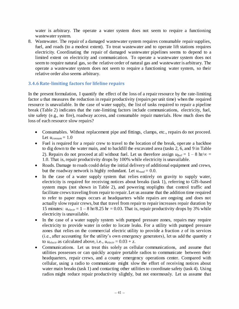
– 41 –
water is arbitrary. The operate a water system does not seem to require a functioning
wastewater system.
8. Wastewater. The repair of a damaged wastewater system requires consumable repair supplies,
fuel, and roads (to a modest extent). To treat wastewater and to operate lift stations requires
electricity. Coordinating the repair of damaged wastewater pipelines seems to depend to a
limited extent on electricity and communication. To operate a wastewater system does not
seem to require natural gas, so the relative order of natural gas and wastewater is arbitrary. The
operate a wastewater system does not seem to require a functioning water system, so their
relative order also seems arbitrary.
3.4.6 Rate-limiting factors for lifeline repairs
In the present formulation, I quantify the effect of the loss of a repair resource by the rate-limiting
factor u that measures the reduction in repair productivity (repairs per unit time) when the required
resource is unavailable. In the case of water supply, the list of tasks required to repair a pipeline
break (Table 2) indicates that the rate-limiting factors include communications, electricity, fuel,
site safety (e.g., no fire), roadway access, and consumable repair materials. How much does the
loss of each resource slow repairs?
Consumables. Without replacement pipe and fittings, clamps, etc., repairs do not proceed.
Let uconsum = 1.0
Fuel is required for a repair crew to travel to the location of the break, operate a backhoe to dig down to the water main, and to backfill the excavated area (tasks 2, 6, and 9 in Table
2). Repairs do not proceed at all without fuel. Let us therefore assign ufuel = 1 – 8 hr/ = 1.0. That is, repair productivity drops by 100% while electricity is unavailable.
Roads. Damage to roads could delay the initial delivery of additional equipment and crews,
but the roadway network is highly redundant. Let uroad = 0.0.
In the case of a water supply system that relies entirely on gravity to supply water, electricity is required for receiving notices about breaks (task 1), referring to GIS-based
system maps (not shown in Table 2), and powering stoplights that control traffic and
facilitate crews traveling from repair to repair. Let us assume that the addition time required
to refer to paper maps occurs at headquarters while repairs are ongoing and does not
actually slow repair crews, but that travel from repair to repair increases repair duration by
15 minutes: uelectr = 1 – 8 hr/8.25 hr = 0.03. That is, repair productivity drops by 3% while
electricity is unavailable.
In the case of a water supply system with pumped pressure zones, repairs may require
electricity to provide water in order to locate leaks. For a utility with pumped pressure
zones that relies on the commercial electric utility to provide a fraction z of its services
(i.e., after accounting for the utility’s own emergency generators), let us add the quantity z
to uelectr as calculated above, i.e., uelectr = 0.03 + z.
Communications. Let us treat this solely as cellular communications, and assume that utilities possesses or can quickly acquire portable radios to communicate between their
headquarters, repair crews, and a county emergency operations center. Compared with
cellular, using a radio to communicate might slow the effort of receiving notices about
water main breaks (task 1) and contacting other utilities to coordinate safety (task 4). Using
radios might reduce repair productivity slightly, but not enormously. Let us assume that
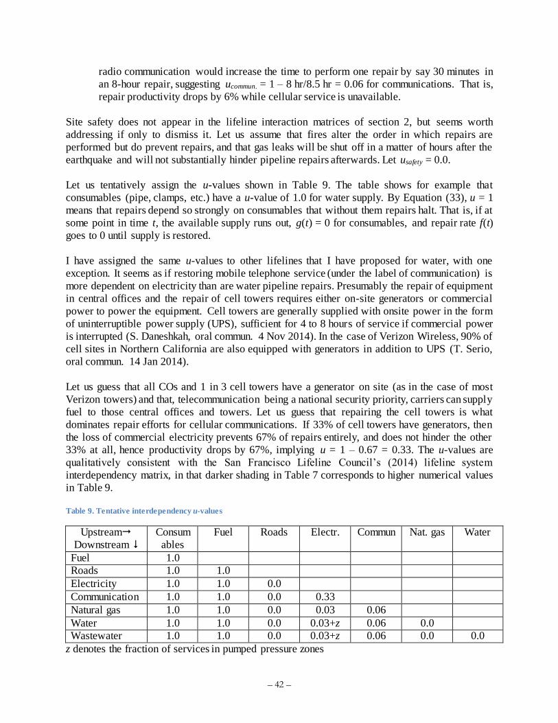
– 42 –
radio communication would increase the time to perform one repair by say 30 minutes in
an 8-hour repair, suggesting ucommun. = 1 – 8 hr/8.5 hr = 0.06 for communications. That is,
repair productivity drops by 6% while cellular service is unavailable.
Site safety does not appear in the lifeline interaction matrices of section 2, but seems worth
addressing if only to dismiss it. Let us assume that fires alter the order in which repairs are
performed but do prevent repairs, and that gas leaks will be shut off in a matter of hours after the
earthquake and will not substantially hinder pipeline repairs afterwards. Let usafety = 0.0.
Let us tentatively assign the u-values shown in Table 9. The table shows for example that
consumables (pipe, clamps, etc.) have a u-value of 1.0 for water supply. By Equation (33), u = 1
means that repairs depend so strongly on consumables that without them repairs halt. That is, if at
some point in time t, the available supply runs out, g(t) = 0 for consumables, and repair rate f(t)
goes to 0 until supply is restored.
I have assigned the same u-values to other lifelines that I have proposed for water, with one
exception. It seems as if restoring mobile telephone service (under the label of communication) is
more dependent on electricity than are water pipeline repairs. Presumably the repair of equipment
in central offices and the repair of cell towers requires either on-site generators or commercial
power to power the equipment. Cell towers are generally supplied with onsite power in the form
of uninterruptible power supply (UPS), sufficient for 4 to 8 hours of service if commercial power
is interrupted (S. Daneshkah, oral commun. 4 Nov 2014). In the case of Verizon Wireless, 90% of
cell sites in Northern California are also equipped with generators in addition to UPS (T. Serio,
oral commun. 14 Jan 2014).
Let us guess that all COs and 1 in 3 cell towers have a generator on site (as in the case of most
Verizon towers) and that, telecommunication being a national security priority, carriers can supply
fuel to those central offices and towers. Let us guess that repairing the cell towers is what
dominates repair efforts for cellular communications. If 33% of cell towers have generators, then
the loss of commercial electricity prevents 67% of repairs entirely, and does not hinder the other
33% at all, hence productivity drops by 67%, implying u = 1 – 0.67 = 0.33. The u-values are
qualitatively consistent with the San Francisco Lifeline Council’s (2014) lifeline system
interdependency matrix, in that darker shading in Table 7 corresponds to higher numerical values
in Table 9.
Table 9. Tentative interdependency u-values
Upstream
Downstream
Consum
ables
Fuel Roads Electr. Commun Nat. gas Water
Fuel 1.0
Roads 1.0 1.0
Electricity 1.0 1.0 0.0
Communication 1.0 1.0 0.0 0.33
Natural gas 1.0 1.0 0.0 0.03 0.06
Water 1.0 1.0 0.0 0.03+z 0.06 0.0
Wastewater 1.0 1.0 0.0 0.03+z 0.06 0.0 0.0
z denotes the fraction of services in pumped pressure zones

– 43 –
3.4.7 Depicting lifeline interaction with an influence diagram
It can sometimes help to depict the relationships among decisions, uncertain quantities, and value
outcomes using an influence diagram. These diagrams, sometimes also called a relevance
diagrams, decision diagrams, and decision networks, are graphical representations of a decision
situation. They can represent a mathematical model that relates the decisions, uncertain quantities,
and uncertain value outcomes with functional relationships. They are commonly used in decision
analysis. They tend to be more compact than decision trees, able to show more information in less
space. The interested reader is referred for more background on influence diagrams to Howard
(1990). The interdependencies implied by Table 9 are depicted in an influence diagram in Figure
10.
In the influence diagram, decisions are depicted in rectangles, uncertain quantities in ovals, and
mathematical dependency by arrows. Time generally flows from left to right or from top to bottom
in an influence diagram; here time flows from left to right. Each arrow starts at a quantity (a
decision or an uncertainty) and points to another quantity. An arrow implies that the second
quantity depends to some extent on the first. Where there is no arrow connecting one quantity to
another, the implication is that neither quantity depends on the other. For example, there is no
arrow from roadway restoration to any of the other lifeline restoration uncertainties. This is not
strictly true, at least according to the San Francisco Lifelines Council (2014) and other lifeline
interaction matrices, but for practical reasons any such dependency can be ignored because the
roadway network is so redundant that it seems unlikely that realistic roadway damage could
significantly impair restoration of other lifelines. There is an arrow corresponding to each nonzero
quantity in the interdependency matrix of Table 9. The arrow is omitted where the corresponding
u-value in Table 9 has a zero value.
The figure omits the dependence of lifeline restoration after aftershock 1 on fuel supply and on
consumable repair resources, but the omission is just for clarity. In practice, or at least in the
calculations performed here, those dependencies exist.
Figure 11 distills the influence diagram to combine all upstream lifelines together and all
downstream lifelines together. The figure also adds value outcomes—the quantities that in the end
the analyst cares about, which in the present case is indirect business interruption loss. In the
canonical influence diagram, value outcomes are shown as hexagon at the right side of the diagram.
Indirect business interruption can be quantified by others as a function of the restoration of the
lifelines; that task of disaster economic is not addressed here.
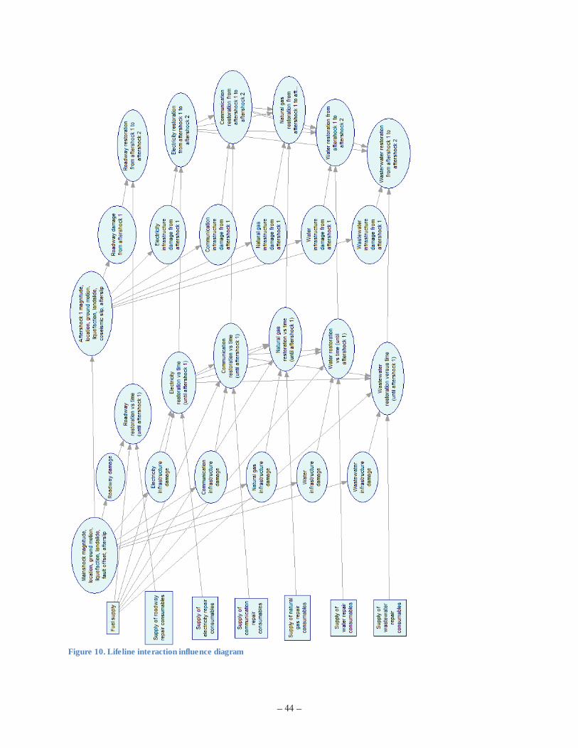
– 44 –
Figure 10. Lifeline interaction influence diagram
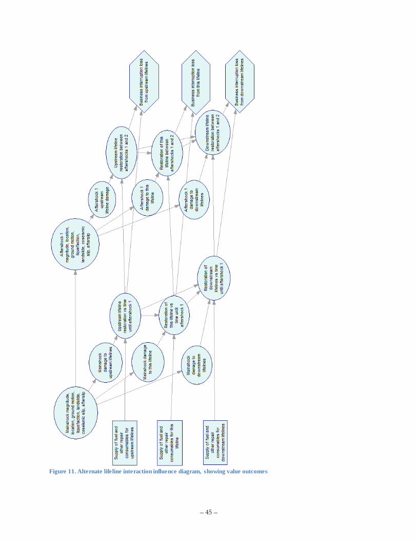
– 45 –
Figure 11. Alternate lifeline interaction influence diagram, showing value outcomes
– 46 –
3.5 Measuring water supply resilience
As proposed by Bruneau et al. (2003), let us view the area above the restoration curve R as a
measure of the loss of resilience: less area means less impact, faster recovery, or both. Recall that
Bruneau et al. (2003) measured R as in Equation (36):
1
0
1
t
R Q t dt (36)
where Q(t) denotes the degree of service as a fraction of full service at time t, and times t = 0 and
t = t1 denote the initiating event (the earthquake) and the time of full restoration, respectively. For
present purposes, let us measure Q(t) as the fraction of all service connections receiving water at
time t, whether treated or not, whether at normal pressure or not (which one can call “wet water,”
as opposed to treated water). Since the present analysis calculates V(t), the number of service
connections receiving water at time t, one can normalize V(t) by the number of service connections,
denoted here by M, and substitute:
1
0
1
tV t
R dtM
(37)
R can be seen as the average number of days a service connection loses service. It will be useful
to estimate the total economic impact of the loss of resilience, which relates more closely to the
number of service-days lost, R∙M:
1
0
t
R M M V t dt (38)
Let us measure the benefit of a mitigation option in terms of the reduction in R∙M relative to some
baseline condition such as as-is conditions:
baseline what if
R M R M R M
(39)
where “what-if” indicates the loss of resilience with the mitigation measure.
Suppose that in some cases, loss of water supply is the sole cause that a home or business loses
function, and the home residents or business occupants experience a financial loss as a
consequence. (Loss of water service caused 18% of business closures after the 1994 Northridge
earthquake, according to Tierney’s 1995 survey.) A household might have temporarily move to a
hotel until water is restored, or a business might suspend operations until water is restored. What
would be the daily cost of lost service?
In the San Francisco Bay Area, moving to a hotel might cost a household on the order of $560 per
day including accommodations, meals, and incidental expenses. (San Francisco Bay Area average
household size is 2.7 [http://goo.gl/NAOnhZ] and the 2016 GSA per diem rate for Oakland is $209
including lodging, meals, and incidental expenses: 2.7∙$209 = $564.) Alameda County contains
140,000 firms (http://goo.gl/b9O19I), which had total sales in 2007 of $81.6 billion, suggesting an
average daily business revenues of $1,600. Considering that Alameda County has 545,000
households (http://goo.gl/b9O19I), the average daily cost of loss of function of a household or
business establishment can be estimated as the weighted average of $560 and $1,600, or $770.
Until an economic analysis is performed, one can take $770 as the average cost of one lost service-
day.

– 47 –
3.6 Optional stochastic simulation methodology
3.6.1 Simulation of earthquake excitation
The present work can be applied to an earthquake planning scenario that requires only a single
realistic outcome, not best, worst, or mean cases or any particular probabilistic outcome. However,
to make the work more generally useful, it is convenient to add features that allow the analyst to
treat earthquake damage to a water supply system as stochastic, i.e., uncertain, random.
I will treat the simulation of the earthquake excitation only superficially; the interested reader is
referred to Chen and Scawthorn (2003) for methods to generate a stochastic set of earthquakes that
are consistent with the seismicity of regional faults, their possible earthquake magnitudes and
rupture locations. In the United States, the National Seismic Hazard Mapping Program (e.g., most
recently Petersen et al. 2014) can offer a model of seismicity.
For each mainshock rupture in the stochastic set, one generates an earthquake sequence of
foreshocks, mainshock, and aftershocks. Ogata (1998) provides a general reference for modeling
aftershocks using an epidemic-type aftershock sequence (ETAS). Field et al. (2013) developed an
ETAS model for California.
Median ground motion and logarithmic standard deviations of ground motion in each earthquake
in the sequence can be calculated using convenient and regionally appropriate ground motion
prediction equations. In the case of the Hayward Fault mainshock, I adopted results of a physics-
based model by Aagaard et al. (2010a, b), but one can also use less-expensive methods. For
example, for shallow crustal earthquakes in active tectonic regimes, one can use the NGA West 2
ground motion prediction equations; see Boore et al. (2014).
Ground motion is uncertain and spatially correlated. Here, uncertain means that ground motion it
can be higher or lower than the median predicted by the ground motion prediction equations,
potentially many times higher and lower. It is important to treat that variability about the median:
ignoring it will tend to bias damage and loss estimates low. One can simulate a properly varying
and spatially correlated field of ground motion using Jayaram and Baker (2009).
3.6.2 Simulation of pipeline vulnerability
Vulnerability of buried pipeline is uncertain. To simulate break rate in buried pipe subjected to
wave passage, landslide, and liquefaction, one can draw two sample u1 and u2 from a U(0,1)
uniform distribution (i.e., equally likely to take on any value between 0 and 1), and simulate break
rates in buried pipeline by substituting u for the nonexceedance probability p. For example, in the
present adaptation of Eidinger’s (2001) model, Equation (22), one substitutes u for p as shown in
Equations (40) and (41):
1 2~ ~ 0,1u u U (40)

– 48 –
1
1 2 1 1
1
2 2
, , , 1 0.00187 exp 1.15
1.88 exp 0.74
L L
L
R PGV P u u P K PGV u
K P u
(41)
The symbol ~ here means “is a sample taken from the distribution.” Equation (40) says, “draw a
sample u1 and another sample u2 from a U(0,1) distribution.” Each assignment can be carried out
in a spreadsheet using, for example Microsoft Excel’s rand() function, which produces a sample
U(0,1) and changes it each time the spreadsheet is recalculated.
The simulation equations assume that vulnerability to wave passage varies independently from
vulnerability to ground failure, but that the intra-system vulnerability for each peril is completely
correlated. That is, all wave-passage break rates within a system will be uniformly higher or lower
than average in a given system, and all ground-failure break rates within a system will be uniformly
higher or lower than average in a given system.
3.6.3 Simulation of damage to buried pipeline
Next, simulate the damage to the buried water supply pipeline system. The simulation treats the
break rates as uncertain as shown in Equation (41). Let us denote by ri the simulated break rate in
each segment of pipe. The simulation then treats the number of leaks or breaks in any given
segment of buried pipe i as distributed with a Poisson distribution whose mean rate r is estimated
from Equation (26) for summand i. The Poisson distribution is a discrete probability distribution
that expresses the probability of a given number of events occurring in a fixed interval of time or
space if these events occur with a known average rate and independently of the time or distance
between events. In this case, the events are breaks or leaks and the fixed interval of space is the
length of the pipe segment.
So, conditioned on the mainshock shaking and ground failure values (here, PGV and PL) at each
pipe segment’s midpoint, and on the vulnerability function assigned to each component (here, K1,
K2, and L values for each pipeline segment), the simulation assumes that the probability of exactly
y breaks on segment i (y {0, 1, 2, ... }) is given by Equation (42). The probability that y or fewer
breaks occur is given by Equation (43), which is the cumulative distribution function for the
Poisson distribution with rate parameter ri.
exp
!
y
i i
i
r rP Y y
y
(42)
0
exp
!
nyi i
i
n
r rP Y y
n
(43)
max :i i iY y u P Y y (44)
To simulate a particular number of breaks in segment i, one draws a sample ui from a uniform
distribution ui ~ U(0,1) and solves Equation (44) for y. The equation inverts the cumulative
distribution function of a Poisson distribution with rate ri at ui to produce the number of simulated
breaks on segment i. I know of no closed-form expression for the value of Yi in Equation (44), but
simulation software such as @Risk can perform the simulation.

– 49 –
Equation (44) does not include breaks at where the pipeline crosses the fault. To deal with pipe
breakage at fault offset, let us take df from Equation (26) as uncertain. It is common to take fragility
functions as approximated by a lognormal cumulative distribution function, so absent a better
empirical or analytical model, let us do so here, and assume a median value θ = 4 inches and
logarithmic standard deviation β = 0.6. I propose this particular median value because it seems like
a reasonable threshold in light of Eidinger’s liquefaction vulnerability function in Figure 7. I
propose this particular logarithmic standard deviation because it reflects a relatively large degree
of uncertainty, compared with other fragility functions such as those in FEMA P-58 (Applied
Technology Council 2012).
To use these fragility parameters to model pipe breaks due to fault offset, for each segment i that
crosses the fault, add 0 or 1 pipe breaks per Equation (45). In the equation Zi denotes either 0 or 1
pipe breaks produced by fault offset at segment i, I() is the indicator function (1.0 if the term in
parentheses is positive, 0.0 if negative), () is the standard normal cumulative distribution
function evaluated at the term in parentheses, di is the fault offset distance where the fault intersects
pipeline segment i, θ and β are as just defined, and ui is another sample from a uniform distribution
ui ~ U(0,1). To explain the equation, the term gives the probability that segment i is broken. If ui is less than that probability, then the simulation says that that segment is broken, that is, that that
segment’s uncertain capacity to resist fault offset was less than di.
ln i
i i
dZ I u
(45)
Finally, one can sum over all pipeline segments to simulate the total simulated number of breaks
W, as in Equation (46):
1
n
i i
i
W Y Z
(46)
3.6.4 Simulation of restoration
As shown in Figure 9, time to repair a break or leak is uncertain and approximately lognormally
distributed. Let us use the parameters derived from Schiff’s data for small-diameter pipe and the
assumed parameters for large-diameter pipe as recapped in Table 10. Repair duration for a single
break can be estimated using Equation (47). In the equation, ui is a random number drawn from a
uniform distribution, ui ~ U(0,1), and is not the same ui value as used elsewhere in this section.
Table 10. Uncertain pipe-repair duration
Median,
θ (hr)
Logarithmic standard
deviation, β
Basis
Small diam (<20 in) 6.1 0.58 Schiff (1988)
Large diam (≥ 20 in) 16 0.6 Schiff (1988) and judgment
1
0, expi id u (47)
It is problematic to offer a stochastic model for number of services lost as a function of damage
(the serviceability index), partly because the use of the serviceability index seems so tenuous to

– 50 –
begin with. Treating it as uncertain with a specified model seems like illusory thoroughness —
cutting the baloney too thin. However, until a better model comes along, let us treat the initial level
of service V0 (now an uncertain quantity rather than a deterministic value) as beta-distributed with
bounds 0 and 1, mean value given by Equation(48), and coefficient of variation = 0.5 (this last by eye from Figure 4). (For the reader who is unfamiliar with the beta distribution, it is a commonly
used probability distribution for an uncertain quantity that can take on a value only between two
bounds, such as between 0 and 1, and has a specified mean and standard deviation.) The parameters
of the beta distribution, denoted here by α and β, can be calculated as shown in Equations (50) and
(51). The inverse cumulative distribution function for the beta distribution is approximated by the
inverse of the Kumaraswamy cumulative distribution function (Kuramaswamy 1980, Jones 2009),
which is easier to calculate. One generates a sample of a uniform distribution u ~ U(0,1) and
evaluates the inverse cumulative distribution function of the Kumaraswamy distribution as shown
in Equation (52) to produce a sample of the initial level of service V0.
ln
1
M s r
r
L qM
b
(48)
0.5 (49)
2
1
(50)
1
1
(51)
1
11
0 1 1V F u u
(52)
The rate-limiting factors of section 3.4.6 can similarly be treated as beta-distributed (which one
can approximate using the Kumaraswamy distribution as before) bounded by 0 and 1, with means
as proposed in Table 9. Values that are assigned 0 or 1 in the table can be taken as certain, i.e.,
with coefficient of variation equal to 0. Rate-limiting factors greater than 0.0 and less than 1.0 are
uncertain; let us take their coefficient of variation as substantial, say 1.0. That is, let
u = a sample of the (possibly uncertain) rate-limiting factor
m = expected value of the rate-limiting factor, from Table 9
d = assumed coefficient of variation of the rare-limiting factor
d = 1 m {0,1} (the symbol means “is not a member of the set listed here”)
= 0 otherwise
v = a sample of a uniform distribution bounded by 0 and 1, i.e., v ~ U(0,1). I use v here for
the sample uniform variate because u is already in use in this step.
Then,
– 51 –
2
1 ma m
d
d 0 (53)
1
1b am
d 0 (54)
11
1 1 0
0, i.e., 0,1
ab
u v d
m d m
(55)
The symbol means “is a member of the set listed here, i.e., inside the curly brackets.”
3.7 Accounting for afterslip and aftershocks
Aftershocks produce new damage to a system that may be only partially repaired. To estimate
number of required repairs after an aftershock, let us estimate new damage as if it occurred to a
pristine system. Add the number of repairs that have not yet been completed, and recommence the
calculation of services restored by the nth repair and time required to perform the nth repair.
Afterslip can increase the deformation on a pipeline segment at a fault crossing where the pipeline
is already strained by coseismic (and possibly preseismic) slip. One way to model pipeline damage
due to afterslip is to treat the pipe as having a fixed capacity to resist deformation.
When the coseismic slip plus afterslip at a point where a pipeline segment crosses the fault reaches
that capacity, the pipe breaks. The capacity can be treated as having a deterministic value or a
probabilistic value. As discussion in section 2, the capacity in reality depends on the material, pipe
diameter, jointing, and sense of deformation, i.e., whether in tension, shear, or compression. For
simplicity for present purposes I propose to treat the capacity as having a single scalar quantity for
all materials, diameters, etc., per Equation (24) for a deterministic model or Equation (45) for a
stochastic model.
3.8 Adjusting Hazus’ lifeline restoration model
3.8.1 Why one might need to adjust the restoration curves offered by Hazus-MH
As discussed in section 2, Hazus-MH is FEMA-funded software to perform risk analysis for
earthquakes, hurricanes, and floods in the United States. Hazus performs hazard analysis, damage
analysis, loss analysis and recovery analysis including repair costs, life-safety impacts, and the
duration and economic losses resulting from loss of function. It includes built-in asset definitions
for virtually the entire built environment of the US, including lifelines, and encodes other
restoration parameters such as the number of workers available to perform repairs. It is a very
powerful tool.
In the author’s experience, loss-estimation software, not matter how advanced, becomes obsolete
soon after its release. Users see that the software’s capability extends to X and soon conceive of a
new need X that that the software does not satisfy. Hazus-MH is like that. The new need
identified here is the ability to treat lifeline interactions and aftershocks. Hazus-MH is currently
closed source, so the analyst who wants to add the ability to treat lifeline interaction and

– 52 –
aftershocks cannot do so by changing the source code, although many parameters can be changed.
How can one modify the outputs, using principles presented here to do so?
3.8.2 Adjusting Hazus’ estimates of lifeline restoration to account for repair crews
Before addressing lifeline interaction and aftershocks, let us consider the situation where a Hazus -
MH analysis has already been performed and the user realizes that an important adjustable
parameter—the number of workers available to perform repairs—was wrong? The Hazus-MH
default value for the number of water-supply pipeline repair workers available in each county
appears to be 100 regardless of the size of the county, which may be far from accurate in many
cases. If the analyst has a supposedly better estimate of the number of repair workers in a particular
county, how can the analyst adjust Hazus’s restoration estimate to account for that better estimate
of repair crews after the fact? Let us assume that repair progress increases linearly with number of
repair crews. It seems uncontroversial to adjust Hazus’ estimated restoration curve to account for
a different estimate of repair-crew resources as shown in Equation (56):
00
ˆ
t
q t dV tV dt
q dt
M
(56)
where
1
1
1
ˆ ˆ ˆ; 1, 2,...5
ˆ2,3, 4,5
j j j
j j
j
dV t V t V tj
dt t t
dV tj
dt
(57)
Let us also assume
6V̂ t M (58)
where
ˆjV t = Hazus’ estimate of the number of service connections with water service at time tj
assuming default values of the number of workers, for the geographic area of interest, e.g.,
a county
j = an index to points in time after the earthquake, j {1, 2, ... 6}
tj = time after the earthquake, tj {1, 3, 7, 30, 90, 540} days, where t6, 540 days, is added to Hazus’ basic list of 5 points in time (1, 3, 7, 30, 90) days to account for the fact that Hazus-MH
might report incomplete restoration at 90 days, and the analyst may need to evaluate
restoration after 90 days
q(t) = analyst’s estimate of the number of water pipeline repair workers available in the county at
time t
q0 = Hazus default value used in the analysis (e.g., 100)
M = number of service connections in the geographic area of interest (a county)
The inequality in Equation (57) is necessary in case 1ˆ
jV t = M, i.e., the unadjusted Hazus
estimate of restoration is complete in the time between tj and tj+1, which would produce an
unrealistically low restoration slope.

– 53 –
Let us refer to q(t)/q0 as the repair-crew availability factor, and let us refer to V(t) as the repair-
crew-adjusted estimate of restoration before accounting for lifeline interaction. Equation (56) says
that the pace of repairs at time τ is estimated as Hazus’ estimate (the derivate gives the rate of
restoration, i.e., services restored per unit time), increased by the repair-crew availability factor,
i.e., to account for the analyst’s estimate of the correct number of repair workers ava ilable at time
τ, and integrated from time 0 to time t.
For the special case of constant q(t), let us substitute the constant q for q(t). Given constant q and
piecewise linear restoration V(t) to go with Hazus’ limited set of V̂ t values, one can evaluate
Equation (56) to evaluate the repair-crew-adjusted estimate of restoration before accounting for
lifeline interaction as shown in Equation (59):
1
1 1
1 0
ˆ1,2,3,4,5
jk
j k k
k
dV tqV t V t t t j
q dt
M
(59)
3.8.3 Accounting for lifeline interaction in Hazus-MH
Hazus-MH’s restoration curves do not consider lifeline interaction. As of this writing, Hazus-MH
evaluates restoration at five points in time after an earthquake: 1, 3, 7, 30, and 90 days. Let us
further modify the restoration rate from Equation (56) as shown in Equation (60):
1
1 1n
i i
i
dV t dV tu g t
dt dt
(60)
where
0
0
t dVV t V t d
d
(61)
ui is as previously defined (see Table 9), and
gi(t) is as defined in Equation (31), i.e., the flow of rate-limiting factor i divided by the pre-
earthquake flow. In the case of a lifeline, g is the fraction of service connections in upstream
lifeline i receiving service at time t, after accounting for lifeline interaction with their
upstream lifelines. In the case of consumable repair supplies, g is the flow of repair supplies
as a fraction of the amount needed.
The product in Equation (60) is just another factor that modifies the restoration rate, like q/q0 in
Equation (59). We can include lifeline interaction by multiplying the restoration rate by this
additional factor, as in Equation (62):
1
1 1
1 10
ˆ1 1 1,2,3,4,5
j nk
j i i k k
k i
dV tqV t V t u g t t t j
q dt
M
(62)
3.8.4 Accounting for aftershocks in Hazus-MH

– 54 –
To adjust Hazus-MH results to account for an aftershock occurs, let us reduce V(t) by the amount
of service estimated lost when the virgin system is damaged by aftershock j, i.e.,
0jV t V t M V (63)
Where M denotes the number of services in the county and Vj(0) denotes the number of service
connections receiving lifeline service immediately after the aftershock, as estimated by Hazus-MH
for the virgin system, i.e., as if the system were undamaged at the time of the aftershock.
3.9 Mitigation options
Let us consider only two mitigation options: one to reduce a water utility’s reliance on commercial
fuel, another to reduce the quantity of brittle pipe or pipe running through liquefiable soil. Other
mitigation options certainly exist.
3.9.1 Fuel plan
A utility can reduce its reliance on commercial fuel supplies by installing above-ground fuel
storage tanks in its service centers. An above-ground storage tank of 3,000 gallons such as shown
in Figure 12 would be sufficient for 10 repair crews to operate for a week or more before needing
to be refilled. The above-ground fuel tank in Figure 12 has a fuel transfer pump (the red box) that
can be powered by a small vehicle-mounted generator that a repair truck can easily carry. An
electrical contractor can be dispatched connect a secondary electrical generator to a fuel island in
a few hours. If trucks are regularly refilled at the end of each day, the time required to connect a
fuel pump to a generator need not affect repair operations. Alternatively, service centers can be
equipped with an emergency generator and switchgear to power fuel pumps in the case of
commercial electric failure. At least one large California utility carries such a generator on all its
repair vehicles and maintains a fuel supply of up to 3,000 gallons or more at its service centers ,
and has installed emergency generators at several of its service centers.

– 55 –
Figure 12. Above-ground petroleum tank
3.9.2 Pipe replacement
With an aggressive pipe-replacement program, a water utility can realistically replace 1 percent of
buried pipe per year, although lower replacement rates are more common. For example, San
Francisco plans to replace 1.3 percent of its water distribution pipe (15.5 miles of a its 1,230-mile
distribution system) in FY 2016 (https://goo.gl/iRtu4w, https://goo.gl/SmjBwm) With a sustained
program that focuses on replacing brittle pipe (e.g., cast iron and asbestos cement), or pipe installed
in liquefiable soil, a utility could replace the majority of its brittle or vulnerable system within a
few decades.
3.10 Summary of the methodology
To recap, the methodology proposed here models damage and restoration of buried pipelines
subject to earthquake shaking (called wave passage) and ground failure (liquefaction, landslide,
and surface rupture of the fault). Briefly, its steps are as follows.
1. One acquires maps of ground motion, especially peak ground velocity and ground failure
(liquefaction, landslide, and fault offset), for each earthquake of interest. One then carries
out the following steps.

– 56 –
2. Equation (26) estimates r, the number of repairs required because of earthquake damage,
using basic loss-estimation principles.
3. Equation (27) estimates V0, the number of service connections that have service available
immediately after the earthquake. It assumes that the serviceability index (a measure of
water-supply pressure loss as a function of water-supply pipeline breaks per km of pipe)
can be used as a proxy to estimate the fraction of services available. It would be desirable
to replace this assumption, but doing so seems to require hydraulic modeling that would
make the present analysis prohibitively time consuming.
4. Equation (30) estimates V(n), the number of services available after n repairs have been
completed. It employs a parametric form for service restoration, one that reflects EBMUD
engineers’ strategy to perform the most effective repairs (the ones that restore the most
services per repair) first, and one that generally agrees with experience in the Kobe and
Northridge earthquakes.
5. Equation (35) estimates F(t), the number of services restored by time t. Lifeline interaction
is quantified at this stage via a set of time-independent rate-limiting factors u that indicate
loss of repair productivity resulting from the loss of each upstream lifeline or other required
repair resource. The lifeline interaction model modulates the time-dependent effect of the
loss of required resources with a set of time-dependent factors g(t) that measure the flow
of each resource at time t. One calculates F(t) for each of many points in time, t = 0, t,
2t, etc., where the datum t = 0 refers to the time when the mainshock occurs.
6. To apply these equations to a mainshock, one estimates damage and immediate loss of
service. Then estimate the service restoration and time required to perform the service
restoration for each repair n {1, 2, ... r}. Finally one relates time to number of services available.
7. To account for aftershocks, repeat tasks 2-6, adding the damage that remains unrepaired as
if the remaining damage occurred with the aftershock.
8. To treat the entire model as stochastic (i.e., random, uncertain), simulate pipeline
vulnerability using Equation (41), damage using Equation (42), initial loss of service using
Equation (52), and the rate limiting factors for each upstream resource using Equation (55)
. Carry out tasks 2-7 as before, many times. Each time represents one possible outcome.
Compile the samples of whichever parameter values are of interest and estimate any
moments (mean, variance, etc.) of interest.
9. To account for lifeline interaction in Hazus-MH, apply Equation (61), which adjusts the
slope of the Hazus-calculated restoration curve to account for rate-limiting factors among
upstream lifelines, and then integrates the adjusted slope to produce a new restoration
curve.
10. To account for aftershocks in Hazus-MH, apply Equation (63) after each aftershock, which
reduces each lifeline’s functionality as estimated by Hazus-MH for the virgin system
shaken by the aftershock. One then continues the integration over time using the adjusted
mainshock restoration curve of the previous step.
4. Case study 1: San Jose Water Company
4.1 San Jose Water Company asset definition

– 57 –
Let us exercise the proposed methodology on a real water supply system subjected to the
hypothetical Hayward Fault earthquake sequence. Let us first consider summary features of the
case study system: the San Jose Water Company’s water supply system’s buried pipeline network.
The following statistics are taken from SJWC (2015). SJWC is 150 years old, serves 225,000
service connections, and employs 345 people. It serves 80% of San Jose, 50% of Cupertino, all of
Saratoga, Los Gatos, Monte Sereno, and Campbell, and unincorporated parts of Santa Clara
County. Daily demand for drinking water varies from 85 to 165 million gallons, with an average
daily demand for drinking water of approximately 120 million gallons. It has 2,400 miles (4,000
km) of water pipes (mains), 105 active wells, a 6,500-acre water shed in Santa Cruz Mountains,
96 distribution reservoirs, two surface-water treatment plants, and performs approximately 370
water quality tests each month.
SJWC provided an ArcGIS map of its water supply system. The system map is shown in Figure
13. The map shows 3,959 km of pipe of various types and lengths. Quantities of pipe are
summarized by material in Table 11 and by diameter in Figure 14. In the tables and figures,
“Material” presents a code for pipe material, “Count” means the number of segments of that
material in the system map, “Miles” and “km” refer to the total length of pipe of that material,
“Material description” describes the pipe material, and “Eidinger type” and “ID” refer to the
assumed corresponding vulnerability functions by Eidinger (2001) and their associated
vulnerability factors K1 and K2 from Table 1. Some of SJWC’s pipe does not map well to an
Eidinger type, especially SJWC’s steel pipe, which generally has lead or cement caulk rather than
any of the joint types that Eidinger considers.
Some of the material codes do not appear in SJWC’s glossary of pipe types, and are probably data-
entry errors. I have made a reasonable assumption about the intended meaning, but in any case the
total quantities of these questionable materials are small: 30.2 of 2459 miles, or just over 1%.

– 58 –
Figure 13. SJWC system map

– 59 –
Table 11. SJWC pipe construction, associated with Eidinger (2001) vulnerability functions
Material Count Miles Km Material description1 Eidinger (2001) type2 ID2
AC 7144 398.5 641.3 Asbestos cement Asbestos cement, cement joint 14
BCL 14 0.3 0.4 Bare cement lined steel Welded steel, rubber gasket 10
CCCL 1110 63.0 101.4 Cement mortar coated and lined steel pipe Ditto 10
CI 3913 210.7 339.0 Cast iron Cast iron rubber gasket 4
CL 5 0.0 0.0 Cement-lined steel Welded steel, rubber gasket 10
CU 71 0.9 1.4 Copper Ditto 10
DCCL 136 4.7 7.6 Dimet coated cement lined steel Ditto 10
DCIL 1 0.2 0.3 Ductile iron cement lined Ductile iron rubber gasket 19
DFK 1 0.0 0.0 Dipped & fiberglass-Kraft wrapped (asphalt coated) steel
Welded steel, rubber gasket 10
DICL 16962 789.4 1270.4 Ductile iron cement lined Ductile iron rubber gasket 19
DIMCL 7 0.3 0.5 Dimet coated cement lined steel Welded steel, rubber gasket 10
DS 6 0.3 0.4 Dimet coated steel Ditto 10 FKCL 3643 199.4 320.8 Fiberglass-kraft wrapped cement-lined steel Ditto 10 GALV 72 0.6 0.9 Galvanized steel Ditto 10 GG 9 0.0 0.1 Groove and grip steel Welded steel screwed joint 11
HDPE 14 2.9 4.6 High Density Polyethylene plastic PVC rubber gasket 18
PB 2 0.1 0.1 Polybutylene plastic Ditto 18
PE 5 0.3 0.5 Polyethylene plastic Ditto 18
PP 1 0.0 0.0 Polypropylene plastic Ditto 18
PVC 857 40.2 64.7 polyvinyl chloride plastic Ditto 18
RCP 3 0.0 0.0 Reinforced Concrete Asbestos cement, cement joint 14
S 109 1.7 2.7 Steel Welded steel, rubber gasket 10 SB 232 3.9 6.3 Standard black steel Ditto 10 SG 1 0.0 0.0 Standard galvanized steel Ditto 10 SI 114 5.6 9.0 Sheet Iron Ditto 10 SOMCL 4903 281.8 453.5 Somastic coated cement lined steel Ditto 10 SS 256 8.1 13.0 Standard screw steel Welded steel screwed joint 11
TBD 695 29.4 47.3 Steel Welded steel, rubber gasket 14
WI 12 0.3 0.5 Wrought iron Cast iron, cement joint 1
WS 598 32.0 51.5 Wrapped steel unlined Welded steel, rubber gasket 10
WSCL 6353 384.5 618.8 Wrapped steel cement lined Ditto 10 ZCCL 5 0.2 0.3 Zinc coated cement lined welded steel Ditto 10 Total 2,459 3,957
1 Descriptions in italics are assumptions 2 Assumed corresponding vulnerability function from Table 1

– 60 –
Figure 14. SJWC pipe quantities by diameter
4.2 San Jose Water Company hazard analysis The Hayward Fault earthquake sequence considered here begins with a Mw 7.0 mainshock on the
Hayward Fault, with an epicenter near Oakland, CA and rupturing the north and south segments
of the fault from a point under San Pablo Bay at the north end to a point near Hayward CA at the
south end. It is followed by a hundreds of aftershocks of magnitude 2.5 or greater. Of these
0
200
400
600
800
1000
1200
0
250
500
750
0 12 24 36 48
Len
gth
of
pip
e, k
m
Len
gth
of
pip
e, m
iles
Pipe diameter, inches

– 61 –
aftershocks, 16 are of magnitude 5.0 or greater. Table 12 summarizes the day, location, label, and
magnitude of each event. In the table, day 1 corresponds to 18 April 2018.
Table 12. Hayward Fault earthquake sequence
Day Epicenter Label Mag
1 Oakland Mainshock 7.05
1 Union City uc523 5.23
1 San Pablo sp504 5.04
12 Fairfield ff558 5.58
15 Fremont fr51 5.10
32 Oakland ok542 5.42
40 Palo Alto pa62 6.21
40 Menlo Park mp552 5.52
41 Palo Alto pa569 5.69
41 Atherton at511 5.11
67 Palo Alto pa522 5.22
74 Palo Alto pa526 5.26
166 Cupertino cu64 6.40
166 Mountain View mv598 5.98
166 Sunnyvale sv535 5.35
166 Santa Clara sc509 5.09
492 Palo Alto pa501 5.01
Figure 15, Figure 16, and Figure 17 show the system map overlain with mainshock peak ground
velocity, liquefaction probability, and landslide probability, respectively. The mainshock surface
rupture does not reach SJWC’s system, so it does not appear in the figures. Figure 18 shows peak
ground velocity contours in a M 6.4 aftershock that occurs on day 166, i.e., 5 months after the
mainshock.

– 62 –
Figure 15. SJWC system map with mainshock peak ground velocity
Figure 16. SJWC system map with liquefaction probability

– 63 –
Figure 17. SJWC system map with landslide probability
Figure 18. SJWC system map with M 6.4 Mountain View aftershock PGV contours (increments of 0.08 m/sec)
4.3 San Jose Water Company damage analysis

– 64 –
Table 13 summarizes mean damage to San Jose Water Company buried pipeline in the mainshock
(1,054 repairs). Aftershocks continue to aggravate damage, contributing 903 more repairs: 29 more
in large-diameter pipe and 873 more in small-diameter pipe. See Table 14 for the expected value
of number of pipe repairs by event in the sequence and Table 15 for subtotals by day. In those
tables, “large diameter” means at least 20 inches. Table 16 summarizes the expected value of the
number of repairs by material, summing damage over the entire earthquake sequence. The table
shows that the plurality of repairs are in asbestos cement pipe (481 breaks), and although the next-
largest contributor is ductile iron pipe (470 breaks), repairs are disproportionately from AC, with
an expected value of 0.23 repairs per 1000 linear feet of pipe (0.75 per km), versus 0.11 per 1000
lf (0.37 per km) from ductile iron. The unsurprising implication is that it is better to have ductile
iron pipe than asbestos cement water pipe.
Table 13. Mainshock mean damage estimate in San Jose Water Company buried pipeline
Mean number of repairs 1,054
Repairs/km pipe 0.27
Due to wave passage 665 (63%)
Due to liquefaction 345 (33%)
Due to landslide 44 (4%)
Large diameter (≥ 20 in diam) 30 (3%)
Small diameter (< 20 in diam) 1024 (97%)
Breaks 294 (28%)
Leaks 760 (72%)

– 65 –
Table 14. Estimated number of leaks and breaks in SJWC buried pipeline in the Hayward Fault sequence
Name Day Epicenter Mag Leaks +
breaks
Lg diam Sm diam
Mainshock 1 Oakland 7.05 1,054 30 1024
uc523 1 Union City 5.23 34 1 33
sp504 1 San Pablo 5.04 6 0 6
ff558 12 Fairfield 5.58 2 0 2
fr51 15 Fremont 5.10 47 1 46
ok542 32 Oakland 5.42 30 1 29
pa62 40 Palo Alto 6.21 102 3 99
mp552 40 Menlo Park 5.52 30 1 29
pa569 41 Palo Alto 5.69 58 2 56
at511 41 Atherton 5.11 30 1 29
pa522 67 Palo Alto 5.22 47 2 45
pa526 74 Palo Alto 5.26 48 2 46
mv598 166 Mountain View 5.98 93 3 90
cu64 166 Cupertino 6.40 172 6 166
sv535 166 Sunnyvale 5.35 73 2 71
sc509 166 Santa Clara 5.09 102 3 98
pa501 492 Palo Alto 5.01 29 1 28
Total 1,957 59 1,897
Table 15. Total leaks and breaks by day
Day Leaks +
breaks
Lg diam Sm diam
1 Total 1,094 31 1,063
12 Total 2 0 2
15 Total 47 1 46
32 Total 30 1 29
40 Total 132 4 127
41 Total 88 3 85
67 Total 47 2 45
74 Total 48 2 46
166 Total 440 14 426
492 Total 29 1 28
Grand Total 1,957 59 1,897
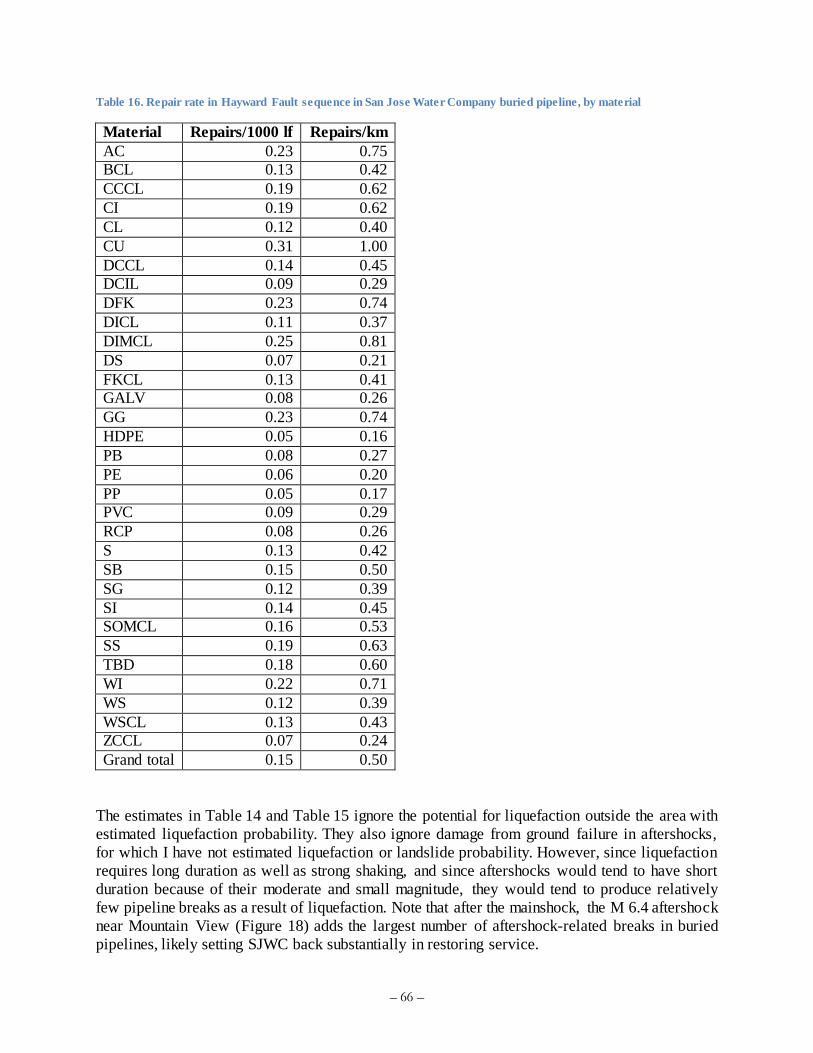
– 66 –
Table 16. Repair rate in Hayward Fault sequence in San Jose Water Company buried pipeline, by material
Material Repairs/1000 lf Repairs/km
AC 0.23 0.75
BCL 0.13 0.42
CCCL 0.19 0.62
CI 0.19 0.62
CL 0.12 0.40
CU 0.31 1.00
DCCL 0.14 0.45
DCIL 0.09 0.29
DFK 0.23 0.74
DICL 0.11 0.37
DIMCL 0.25 0.81
DS 0.07 0.21
FKCL 0.13 0.41
GALV 0.08 0.26
GG 0.23 0.74
HDPE 0.05 0.16
PB 0.08 0.27
PE 0.06 0.20
PP 0.05 0.17
PVC 0.09 0.29
RCP 0.08 0.26
S 0.13 0.42
SB 0.15 0.50
SG 0.12 0.39
SI 0.14 0.45
SOMCL 0.16 0.53
SS 0.19 0.63
TBD 0.18 0.60
WI 0.22 0.71
WS 0.12 0.39
WSCL 0.13 0.43
ZCCL 0.07 0.24
Grand total 0.15 0.50
The estimates in Table 14 and Table 15 ignore the potential for liquefaction outside the area with
estimated liquefaction probability. They also ignore damage from ground failure in aftershocks,
for which I have not estimated liquefaction or landslide probability. However, since liquefaction
requires long duration as well as strong shaking, and since aftershocks would tend to have short
duration because of their moderate and small magnitude, they would tend to produce relatively
few pipeline breaks as a result of liquefaction. Note that after the mainshock, the M 6.4 aftershock
near Mountain View (Figure 18) adds the largest number of aftershock-related breaks in buried
pipelines, likely setting SJWC back substantially in restoring service.

– 67 –
Figure 19 presents a heat map of break rate in the Hayward Fault mainshock. Colors indicate mean
breaks per km2. A warmer color indicates greater concentration of damage.
To be clear, if any additional emphasis is needed, this heatmap shows estimated break rates in one
scenario earthquake—the Hayward Fault mainshock—not all possible earthquakes, not even all
possible M 7.0 earthquakes on the Hayward fault. Different earthquakes produce different damage
patterns. However, the point of a scenario is to understand what might realistically happen, and a
heatmap makes a possible outcome more tangible, more useful for planning purposes. By planning
for one scenario, one becomes more prepared for what actually happens, which will invariably
differ from the scenario.
To return to the map: it unsurprisingly shows greater damage near the fault and on soil with high
liquefaction probability, with maximum values approaching 12 breaks per km2. Figure 20 shows
an analogous map for the M 6.4 Cupertino aftershock. The color scale is shifted to be informative.
Damage rates just exceed 1 break per km2 in the aftershock in the neighborhoods along the northern
edge of the SJWC service area. Figure 21 shows the heatmap for the entire sequence, with damage
rates of approximately 15 per km2 in the northeastern portion of the service area.
Figure 19. Buried water pipeline damage heatmap for the Hayward Fault mainshock in SJWC's service area

– 68 –
Figure 20. Buried water pipeline damage heatmap for Cupertino M 6.4 aftershock in SJWC's service area
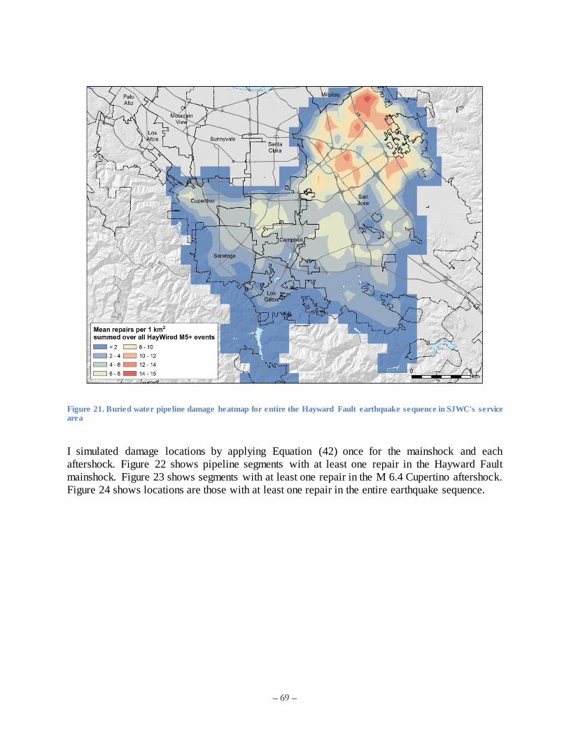
– 69 –
Figure 21. Buried water pipeline damage heatmap for entire the Hayward Fault earthquake sequence in SJWC's service area
I simulated damage locations by applying Equation (42) once for the mainshock and each
aftershock. Figure 22 shows pipeline segments with at least one repair in the Hayward Fault
mainshock. Figure 23 shows segments with at least one repair in the M 6.4 Cupertino aftershock.
Figure 24 shows locations are those with at least one repair in the entire earthquake sequence.

– 70 –
Figure 22. Simulated repairs in SJWC buried pipelines in Hayward Fault mainshock
Figure 23. Simulated repairs in SJWC buried pipelines in Cupertino M 6.4 aftershock
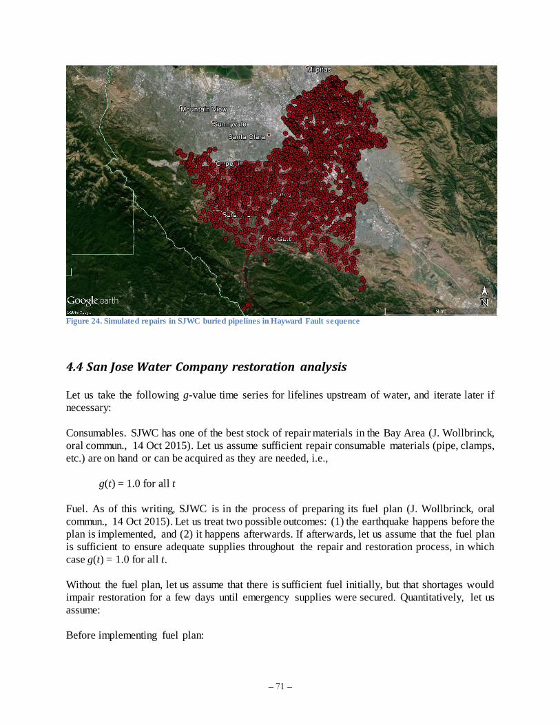
– 71 –
Figure 24. Simulated repairs in SJWC buried pipelines in Hayward Fault sequence
4.4 San Jose Water Company restoration analysis
Let us take the following g-value time series for lifelines upstream of water, and iterate later if
necessary:
Consumables. SJWC has one of the best stock of repair materials in the Bay Area (J. Wollbrinck,
oral commun., 14 Oct 2015). Let us assume sufficient repair consumable materials (pipe, clamps,
etc.) are on hand or can be acquired as they are needed, i.e.,
g(t) = 1.0 for all t
Fuel. As of this writing, SJWC is in the process of preparing its fuel plan (J. Wollbrinck, oral
commun., 14 Oct 2015). Let us treat two possible outcomes: (1) the earthquake happens before the
plan is implemented, and (2) it happens afterwards. If afterwards, let us assume that the fuel plan
is sufficient to ensure adequate supplies throughout the repair and restoration process, in which
case g(t) = 1.0 for all t.
Without the fuel plan, let us assume that there is sufficient fuel initially, but that shortages would
impair restoration for a few days until emergency supplies were secured. Quantitatively, let us
assume:
Before implementing fuel plan:

– 72 –
g(t) = 1.0 for 0 ≤ t < 3 days
g(t) = 0.25 for 3 ≤ t < 7 days
g(t) = 1.0 for t > 7 days
After implementing fuel plan:
g(t) = 1.0
Electricity. PG&E expects to restore power throughout the Bay Area within 1 week. Let us assume
therefore that in practice that means 999 out of 1000 customers are receiving power by the end of
day 7 in a M 7 earthquake, or 2 days after a M 6+ aftershock. Quantitatively, let us therefore take
g(t) = 1 – exp(-0.987t), t measured in days after the mainshock
g(t) = 1 – exp(-3.45t), t in days after the aftershocks on days 40 and 166
Communication. SJWC has battery powered radios for its repair crews that reach almost its entire
service area. Let us assume that communication to facilitate coordination between utilities will be
such a high priority that coordination will not be a constraint. Let us therefore assume
g(t) = 1.0
Crews. SJWC personnel estimated that they could realistically field between 20 and 25 crews on
a work basis of 12 hours on and 12 hours off. Let us therefore take a(t) = 0.5 and c(t) = 22 for
purposes of Equation (35).
Figure 25 shows the repair timeline for San Jose Water Company before and after implementing
the fuel-management plan. Figure 26 illustrates the simulated restoration curve. If the Hazus-MH
serviceability index realistically measures the fraction of services receiving any water, as its
reports suggest, then “services available” in Figure 26 measures the fraction of service connections
receiving even small flows. If it means the post-earthquake flow as a fraction of pre-earthquake
flow, then the chart underestimates the number of service connections receiving at least some
water.

– 73 –
Figure 25. Simulated repair timeline of San Jose Water Company, with and without fuel management plan
Figure 26. Simulated service availability of San Jose Water Company, with and without fuel management plan
As discussed earlier, one views the area above the curves in Figure 26 as a measure of resilience:
less area means less impact, faster recovery, or both. The areas above the three curves are measured
in units of service-days. That is, each day of lost water supply to a service connection equates with
one service-day. The areas above the three curves are shown in Table 24: lost service-days under
as-is conditions, with a fuel plan, and under ideal-world conditions, i.e., assuming that all brittle
pipe is replaced before the earthquake. The table shows the lost service-days as a multiple of
number of services, i.e., the average number of days that each service connection is without potable
0
500
1,000
1,500
1 10 100 1000
Rep
air
s re
ma
inin
g
Day
Fuel shortageAftershocks
With fuel plan
0
50,000
100,000
150,000
200,000
250,000
1 10 100 1000
Serv
ices
av
ail
ab
le
Day
Fuel shortage
Aftershocks
With fuel plan

– 74 –
water under as-is conditions, with the fuel plan, and under ideal-world conditions. The difference
between lost service days under as-is and what-if conditions (fuel plan or ideal world) measures
the resilience benefit of the what-if condition: with a fuel plan and if all brittle pipe were replaced
before the earthquake occurred. Figures have been rounded to reduce the impression of excessive
precision.
Table 17. SJWC lost service-days
Condition Lost service-days R∙M Resilience benefit (R∙M) Average lost days R
As-is 940,000 0 4
Fuel plan 750,000 190,000 3
Ideal world 470,000 470,000 2
4.5 Validation of San Jose Water Company restoration analysis
4.5.1 Cross validation with SJWC’s internal damage estimate
By scaling up the number of breaks in the 2014 Napa earthquake, San Jose Water Company
personnel estimated that the Hayward Fault mainshock would cause 1,200 water main breaks to
their own system (J. Wollbrinck written commun. 19 Oct 2015). The estimate follows this logic:
Napa has 370 miles of water main and experienced 120 leaks the first week, and over 170 for the
1st 6 months. Scaling up by system size, SJWC estimates that Napa’s 120 leaks would equate with
850 leaks for SJWC, and 170 would equate with 1200. The South Napa earthquake was weaker
than what is expected for the mainshock imagined here, so that would make a difference. The
similarity between SJWC’s estimates of 850 increasing to 1200 and the ones produced here (1,054
increasing to 1,956) suggests that either both are reasonable or neither is. That the two set of figures
used two different approaches to arrive at basically the same set of numbers tends to support both
being reasonable, rather than neither. In either case, SJWC engineers found the results presented
here to be reasonable (J. Walsh, written commun., 19 Oct 2015), with the exception that
Wollbrinck (written commun. 4 Dec 2015) expected more damage to wrapped steel pipe because
of its age and corrosion susceptibility.
4.5.2 Validation against Northridge, Kobe, and South Napa earthquakes
Jeon and O’Rourke (2005) report that the 1994 Northridge earthquake caused 1,095 breaks or leaks
to buried pipeline operated by the Los Angeles Department of Water and Power, most of the
damage occurring in the San Fernando Valley. Lund et al. (2005) report that repairs took about 1
week. The present calculation suggests that SJWC would take 23 days to repair 1,176 repairs
(mainshock plus 4 aftershocks through day 15), i.e., about 3 times as long for about the same
number of repairs. Lund et al. (2005) do not report the number of crews required to perform those
repairs. Presumably LADWP fielded more crews than SJWC has at its disposal.
Lund et al. (2005) report that, according to M. Matsushita of the Kobe Municipal Waterworks
Bureau, 1,757 breaks and leaks occurred in buried water supply distribution pipe in Kobe after the
1995 Kobe earthquake and that repairs took 10 weeks. The present estimate of 3 weeks to repair

– 75 –
1,176 breaks and leaks suggests 1/3rd the time to repair 2/3rds the breaks and leaks. Thus, in a
sense, Northridge and Kobe bracket the restoration estimates for SJWC presented here.
The City of Napa repaired approximately 120 leaks and breaks in 5 days with approximately 10
crews working 12-hour shifts (Scawthorn 2014), for a repair productivity of approximately 2.4
repairs per crew-day. The present model suggests that, before its fuel plan is implemented, San
Jose Water Company would repair 1,176 breaks and leaks in 26 days with 22 crews working 12-
hour shifts, or 2.1 repairs per crew day, suggesting fairly good agreement.
4.5.4 Cross validation with Hazus-MH
Using Hazus-MH, Seligson estimated restoration of water supply in Santa Clara County. Results
are shown in Table 18. The estimates are for the mainshock only and do not reflect lifeline
interaction. Applying the percentages to the number of SJWC’s customers, one can compare the
two models, as shown in Figure 27.
The present model and Hazus-MH disagree wildly in terms of initial level of service and
restoration time, with the Hazus-MH model estimating a 6 times increase in time to restore service
compared with the present model. Considering the validation against the Napa repair timeline, the
present restoration model seems more plausible than the Hazus-MH restoration model. Why would
Hazus-MH’s restoration model differ so markedly from the present one? The difference can be
partly explained by the user-specified number of repair crews.
Table 18. Hazus-MH estimate of Santa Clara County loss of water supply
Total Households without potable water
households Day 1 Day 3 Day 7 Day 30 Day 90
565,853 #
%
504,596
89.20%
502,302
88.80%
497,394
87.90%
458,220
81.00%
137,185
24.20%

– 76 –
Figure 27. Comparison of the present model with that of Hazus -MH, as applied to SJWC
4.6 San Jose Water Company under ideal-world conditions
Suppose all of the more-vulnerable SJWC buried pipe (e.g., asbestos cement and cast iron) could
be replaced with less-vulnerable pipe (e.g., ductile iron). What would be the benefit in terms of
damage reduction and accelerated recovery? To explore this question, let us assume that all
asbestos cement and cast iron pipe is replaced with ductile iron before the Hayward Fault sequence
occurs. Let us refer to this as the ideal world assumption. Figure 28 plots the restoration curves for
San Jose Water Company’s buried water supply pipelines under the ideal-world assumption.
An SJWC engineer informs SAFRR that SJWC replaces 1%, or 24 miles, of existing water mains
every year. He does not imagine this study being used to change that percentage of replacement,
but they might change their mix of pipes. Their replacement program is based on both
consequences of failure and probability of failure. They consider a multitude of factors and then
apply genetic algorithm software to predict leaks. They will likely add additional weighting to AC
and CI pipe in close proximity to fault lines based on the present work.
0
50,000
100,000
150,000
200,000
250,000
1 10 100 1000
Serv
ices
av
ail
ab
le
Day
HayWired model
with fuel plan
Hazus-MH model
without aftershocks
or lifeline interaction

– 77 –
A B Figure 28. Benefit of replacing AC and CI pipe with ductile iron: A) repairs remaining versus time and B) services available
versus time
4.7 Effect of lifeline interaction and consumable limits Suppose one ignored limitations in fuel and other consumables, and ignored impairment of
electricity, telecommunications, and so on. How much difference do lifeline interaction and
consumable limits make? Without these effects, damage is unaffected, but repairs could potentially
proceed faster. Recall that Equation (34) gives the time τ(n,t) required to perform the nth repair,
which occurs at time t. It can be expressed as a baseline productivity increased by a factor S(t) that
accounts for how lifeline interaction and consumable limits slow repairs, i.e.,
0,d
n t S tw t c t
(64)
where
1
1 1i i
i
S t
u g t
(65)
The first multiplicand in Equation (64) is the baseline productivity, i.e., the time required to
perform the nth repair, without lifeline interaction and consumable limits. The factor S(t), which is
always at least 1.0, increases the repair time to account for lifeline interaction and consumable
limits. Repeating the calculations for San Jose Water Company under as-is conditions but with S(t)
= 1 produces an estimated 740,000 lost service days, about 80 percent of the value estimated
considering lifeline interaction. Viewed another way, lifeline interaction and consumable limits
decrease the calculated water supply resilience in the area served by San Jose Water Company by
25 percent in the Hayward Fault scenario. The factor would vary in other earthquakes, generally
being larger the dependent the utility is on other lifelines and consumables, and the more these
lifelines and consumables are impaired.
5. Case study 2: East Bay Municipal Utility District
5.1 East Bay Municipal Utility District asset definition
0
500
1,000
1,500
1 10 100 1000
Rep
air
s re
main
ing
Day
Fuel shortageAftershocks
With fuel plan
Ideal
world
0
50,000
100,000
150,000
200,000
250,000
1 10 100 1000
Servic
es
ava
ilab
le
Day
Fuel shortage
Aftershocks
With fuel plan
Ideal
world

– 78 –
We can examine a second system subjected to the same hypothetical earthquake sequence, to see
whether the model can produce plausible results twice. This section considers the East Bay
Municipal Utility District’s water supply buried pipeline network.
The following description is largely quoted from Contra Costa Local Agency Formation
Commission (2008) and from conversations with EBMUD. East Bay Municipal Utility District
(EBMUD) provides water and sewage treatment services for an area of approximately 331 square
miles in the eastern side of the San Francisco Bay. EBMUD serves approximately 1.3 million
people in portions of Alameda County and Contra Costa County in California. EBMUD currently
has an average annual growth rate of 0.8% and is projected to serve 1.6 million people by 2030.
As of 2015 it provides water to approximately 390,000 service connections. Approximately
100,000 are located east of the East Bay Hills, the other 290,000, west.
EBMUD's administrative offices, located in Oakland, own and maintain 2 water storage reservoirs
on the Mokelumne River, 5 terminal reservoirs, 91 miles of three separate water transmission
aqueducts, 4,100 miles of water mains (the only part of the system modeled here), 6 water
treatment plants, 29 miles of wastewater interceptor sewer lines and a regional wastewater
treatment facility rated at a maximum treatment capacity of 320 MGD.
EBMUD provided an ArcGIS map of its water supply system. The system map is shown in Figure
29. The map shows 6,698 km (4,162 mi) of pipe of various types and lengths, of which 2,091 km
are located east of the East Bay Hills, the other 4607 km, west. Total quantities of pipe are
summarized by material in Table 19 and by diameter in Table 20. I discretized EBMUD’s system
into segments with an average length of 64 m and a standard deviation of 79 m—short enough that
shaking should vary little between ends of segments. In the tables, “Material” presents a code for
pipe material, “Count” means the number of segments of that material in the system map, “Miles”
refers to the total length of pipe of that material, “Material description” describes the pipe material,
and “Eidinger type” and “ID” refer to the assumed corresponding vulnerability functions by
Eidinger (2001) and their associated vulnerability factors K1 and K2 from Table 1. Some of
EBMUD’s pipe does not map well to an Eidinger type. One of the material codes do not appear in
EBMUD’s glossary of pipe types, and is probably a data-entry error. I have made a reasonable
assumption about the intended meaning, but in any case the total quantity is small: 0.1 miles.
Terentieff et al. (2015) report that 176,000 of 390,000 water services are in pumped pressure zones.
These pressure zones rely on 130 pumping stations, of which 117 (90 percent) have no emergency
generators. Therefore, let us set the parameter z used in the lifeline interaction matrix for EBMUD
to be 0.9176,000/390,000 = 0.41, and uelectr. = 0.41 + 0.03 = 0.44. The factor 0.9 reflects the 90 percent of pumping stations that have no generator. Conceivably EBMUD could install emergency
generators with large fuel tanks at all its pumping stations, in which case we can take uelectr. = 0.03.
Let us take the former as the real-world scenario and the latter as an ideal-world scenario. Let us
also assume that fuel limitations affect EBMUD the same as SJWC, and like SJWC, EBMUD can
optionally develop a fuel plan and storage to ensure that fuel does not limit its ability to perform
pipeline repairs.

– 79 –
Figure 29. EBMUD system map (red) with dividing line (yellow) to approximately separate pipe and services east and west of the East Bay Hills
Table 19. EBMUD pipe construction, associated with Eidinger (2001) vulnerability functions
Code Material, joint1 Count Miles Closest Eidinger (2001) type2 ID2
A Asbestos cement, unrestrained 24543 1136.4 Asbestos cement with cement joint 14
C Cast iron, unrestrained 33747 1322.1 Cast iron with cement gasket 1
D Ductile iron, unrestrained 43 2.1 Ductile iron with rubber gasket 19
F Fusible PVC, welded 30 1.2 Welded steel lap arc welded joint 6
H High density polyethylene, weld 167 8.8 PVC with rubber gasket 18
K Copper, restrained 50 0.7 Welded stl lap arc weld jt sm diam 6
L Reinf concrete cyl., unrestrained 197 14.3 Concrete w steel cylinder cement jt 16
N PVC, unrestrained 8613 380.4 PVC with rubber gasket 18
P3 Pre-tens. conc. cyl., restrained 1 0.1 Concrete w steel cylinder cement jt 16
R Reinf. conc. noncylinder 2 0.0 Concrete w steel cylinder cement jt 16
S Steel, weld 37101 1282.4 Welded steel lap arc welded joint 6,94
T Pre-tens. conc. cyl., restrained 127 10.4 Conc w steel cylinder lap arc weld 15
W Wrought iron 71 2.7 Cast iron with cement gasket 1
Total 104,692 4,162 1 EBMUD pipe material and description of joint; descriptions in italics are assumptions 2 Closest equivalent corresponding vulnerability function from Table 1 3 One length of 48-inch diam 1927 pipe; P is probably a typo for T 4 ID 6 = small diam (< 20 in), ID 9 = large diam (≥ 20 in)
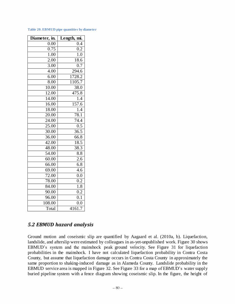
– 80 –
Table 20. EBMUD pipe quantities by diameter
Diameter, in. Length, mi.
0.00 0.4
0.75 0.2
1.00 1.0
2.00 18.6
3.00 0.7
4.00 294.6
6.00 1728.2
8.00 1105.7
10.00 38.0
12.00 475.8
14.00 1.4
16.00 157.6
18.00 1.4
20.00 78.1
24.00 74.4
25.00 0.5
30.00 36.5
36.00 66.8
42.00 18.5
48.00 38.3
54.00 8.8
60.00 2.6
66.00 6.8
69.00 4.6
72.00 0.0
78.00 0.2
84.00 1.8
90.00 0.2
96.00 0.1
108.00 0.0
Total 4161.7
5.2 EBMUD hazard analysis
Ground motion and coseismic slip are quantified by Aagaard et al. (2010a, b). Liquefaction,
landslide, and afterslip were estimated by colleagues in as-yet-unpublished work. Figure 30 shows
EBMUD’s system and the mainshock peak ground velocity. See Figure 31 for liquefaction
probabilities in the mainshock. I have not calculated liquefaction probability in Contra Costa
County, but assume that liquefaction damage occurs in Contra Costa County in approximately the
same proportion to shaking-induced damage as in Alameda County. Landslide probability in the
EBMUD service area is mapped in Figure 32. See Figure 33 for a map of EBMUD’s water supply
buried pipeline system with a fence diagram showing coseismic slip. In the figure, the height of
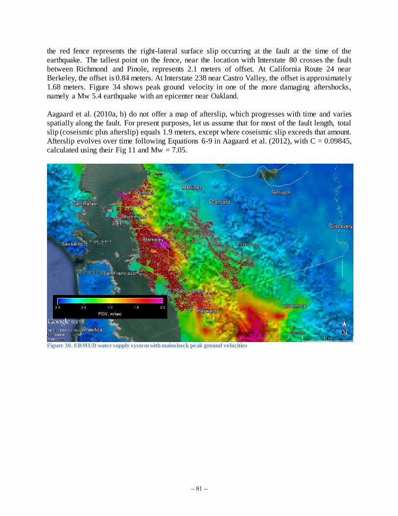
– 81 –
the red fence represents the right-lateral surface slip occurring at the fault at the time of the
earthquake. The tallest point on the fence, near the location with Interstate 80 crosses the fault
between Richmond and Pinole, represents 2.1 meters of offset. At California Route 24 near
Berkeley, the offset is 0.84 meters. At Interstate 238 near Castro Valley, the offset is approximately
1.68 meters. Figure 34 shows peak ground velocity in one of the more damaging aftershocks,
namely a Mw 5.4 earthquake with an epicenter near Oakland.
Aagaard et al. (2010a, b) do not offer a map of afterslip, which progresses with time and varies
spatially along the fault. For present purposes, let us assume that for most of the fault length, total
slip (coseismic plus afterslip) equals 1.9 meters, except where coseismic slip exceeds that amount.
Afterslip evolves over time following Equations 6-9 in Aagaard et al. (2012), with C = 0.09845,
calculated using their Fig 11 and Mw = 7.05.
Figure 30. EBMUD water supply system with mainshock peak ground velocities

– 82 –
Figure 31. EBMUD water supply system with mainshock liquefaction probability
Figure 32. Mainshock landslide probability near EBMUD service area

– 83 –
Figure 33. EBMUD system with fault
Figure 34. EBMUD water supply system with Oakland M 5.42 aftershock PGV contours
– 84 –
5.3 EBMUD damage analysis
Table 21 summarizes the estimated damage to EBMUD pipelines from the scenario mainshock
and aftershocks. Damage in the mainshock includes ground shaking, liquefaction, landsliding, and
surface rupture. Since the available liquefaction map does not include Contra Costa County, I
assume that liquefaction damage in Contra Costa county is proportional to shaking damage in
Contra Costa County, in the same proportions as in Alameda County. As the table illustrates,
aftershock damage ignores landslides, liquefaction, and surface rupture. Note that the mainshock
damage estimate for afterslip assumes that after pipes that are ruptured by fault slip are damaged
a second time by afterslip, EBMUD may decide to either install earthquake-resistant pipe (e.g.,
HDPE pipe or steel pipe with flexible joints that can tolerate extension, compression, and lateral
deformation) or to temporarily install flexible hose until the damaged main can be repaired or
earthquake-resistant pipe can be installed. The table shows that the mainshock produces the
majority of the overall damage, but that after the mainshock, 36% more damage occurs in
aftershocks. Half the mainshock damage is associated with wave passage, the other half to
liquefaction, landsliding, and fault offset.
Table 22 presents the estimated number of leaks plus breaks in EBMUD buried pipeline in each
earthquake of the Hayward Fault sequence. After the mainshock, 6 of 16 aftershocks each produces
at least 100 breaks or leaks, and one produces more than 300, with significant numbers of breaks
and leaks occurring almost 6 months after the mainshock, a point that is made somewhat clearer
by Table 23, which summarizes damage by day after the mainshock. Table 24 details repair rate
over the entire sequence by pipe material. Unsurprisingly, it shows that most damage is in brittle
cast iron and asbestos cement pipe, with damage rates approaching 0.3 per 1,000 lf. Table 25
presents repair rate over the entire sequence by pipe diameter, with most repairs required in 6-inch
and 8-inch diameter pipe, which together represents the majority of pipe in the system.
Figure 35, Figure 36, and Figure 37 present damage heatmaps for EBMUD’s system: they map
mean repairs (estimated per the present methodology) per square kilometer in the mainshock,
most-damaging aftershock (a M 5.4 event with an Oakland epicenter), and the entire sequence.
Damage rates reach 50 repairs per square kilometer along the fault and in zones of high liquefaction
probability. The heatmap for the mainshock shows 20 to 50 breaks per km2 in large areas west of
the fault, and no levels so high east of the fault, consistent with older pipe and higher liquefaction
probability west of the fault. As a further sanity check of the mainshock heatmap, notice that it
shows on the order of 10 leaks or breaks per km2 over an area of about 500 km2, or about the 5,200
leaks and breaks estimated here.
As with the first case study, the heatmaps show estimated break rates in the Hayward Fault
sequence. Different earthquakes would produce different damage patterns. The EBMUD heatmaps
depict a single realistic damage pattern in order to make the scenario more tangible. EBMUD and
its customers, by planning for this scenario, could better prepare for what actually happens, which
will invariably differ in total quantities, spatial distribution of damage, and over time.

– 85 –
Table 21. Hayward Fault mean damage estimate in EBMUD buried pipeline
Mainshock Aftershocks Total
Mean number of repairs 3,916 1,395 5,311
Repairs/km pipe 0.58 0.21 0.79
Due to wave passage 2,063 (53%) 1,395 (100%) 3,458 (65%)
Due to liquefaction 949 (24%) Not calculated 949 (18%)
Due to landslide 179 (5%) Not calculated 179 (3%)
Due to coseismic slip 214 (5%) Not calculated 214 (4%)
Due to afterslip 214 (5%) Not calculated 214 (4%)
Large diameter (≥ 20 in diam) 215 (5%) 84 (6%) 299 (6%)
Small diameter (< 20 in diam) 3,701 (95%) 1,311 (94%) 5,011 (94%)
Breaks 1,235 (32%) 209 (15%) 1,444 (27%)
Leaks 2,681 (68%) 1,185 (85%) 3,866 (73%)
Table 22. Estimated number of leaks plus breaks in EBMUD buried pipeline in the Hayward Fault sequence
Name Day Epicenter Mag Leaks + breaks Diam ≥ 20 in Diam < 20 in
Mainshock 1 Oakland 7.05 3,916 215 3,701
sp504 1 San Pablo 5.04 102 6 96
uc523 1 Union City 5.23 101 6 95
ff558 12 Fairfield 5.58 49 3 46
fr510 15 Fremont 5.1 37 2 35
ok542 32 Oakland 5.42 323 20 304
mp552 40 Menlo Park 5.52 44 3 41
pa62_ 40 Palo Alto 6.2 141 8 133
pa569 41 Atherton 5.11 61 4 57
at511 41 Palo Alto 5.69 44 3 42
pa522 67 Palo Alto 5.22 54 3 51
pa526 74 Palo Alto 5.26 59 4 55
sc509 166 Cupertino 6.4 25 2 24
cu640 166 Mountain View 5.98 173 10 162
sv535 166 Santa Clara 5.09 52 3 49
mv598 166 Sunnyvale 5.35 102 6 96
pa501 492 Palo Alto 5.01 28 2 26
Total 5,311 299 5,011
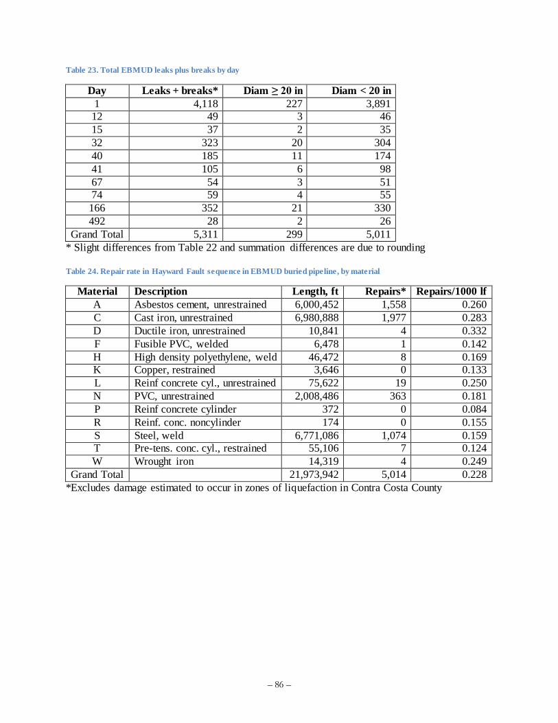
– 86 –
Table 23. Total EBMUD leaks plus breaks by day
Day Leaks + breaks* Diam ≥ 20 in Diam < 20 in
1 4,118 227 3,891
12 49 3 46
15 37 2 35
32 323 20 304
40 185 11 174
41 105 6 98
67 54 3 51
74 59 4 55
166 352 21 330
492 28 2 26
Grand Total 5,311 299 5,011
* Slight differences from Table 22 and summation differences are due to rounding
Table 24. Repair rate in Hayward Fault sequence in EBMUD buried pipeline, by material
Material Description Length, ft Repairs* Repairs/1000 lf
A Asbestos cement, unrestrained 6,000,452 1,558 0.260
C Cast iron, unrestrained 6,980,888 1,977 0.283
D Ductile iron, unrestrained 10,841 4 0.332
F Fusible PVC, welded 6,478 1 0.142
H High density polyethylene, weld 46,472 8 0.169
K Copper, restrained 3,646 0 0.133
L Reinf concrete cyl., unrestrained 75,622 19 0.250
N PVC, unrestrained 2,008,486 363 0.181
P Reinf concrete cylinder 372 0 0.084
R Reinf. conc. noncylinder 174 0 0.155
S Steel, weld 6,771,086 1,074 0.159
T Pre-tens. conc. cyl., restrained 55,106 7 0.124
W Wrought iron 14,319 4 0.249
Grand Total 21,973,942 5,014 0.228
*Excludes damage estimated to occur in zones of liquefaction in Contra Costa County
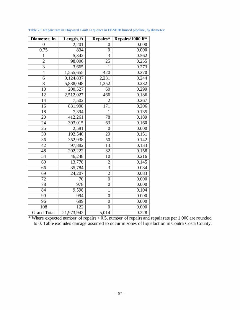
– 87 –
Table 25. Repair rate in Hayward Fault sequence in EBMUD buried pipeline, by diameter
Diameter, in. Length, ft Repairs* Repairs/1000 lf*
0 2,201 0 0.000
0.75 834 0 0.000
1 5,342 3 0.562
2 98,006 25 0.255
3 3,665 1 0.273
4 1,555,655 420 0.270
6 9,124,837 2,231 0.244
8 5,838,048 1,352 0.232
10 200,527 60 0.299
12 2,512,027 466 0.186
14 7,502 2 0.267
16 831,998 171 0.206
18 7,394 1 0.135
20 412,261 78 0.189
24 393,015 63 0.160
25 2,581 0 0.000
30 192,540 29 0.151
36 352,938 50 0.142
42 97,882 13 0.133
48 202,222 32 0.158
54 46,248 10 0.216
60 13,778 2 0.145
66 35,784 3 0.084
69 24,207 2 0.083
72 70 0 0.000
78 978 0 0.000
84 9,598 1 0.104
90 994 0 0.000
96 689 0 0.000
108 122 0 0.000
Grand Total 21,973,942 5,014 0.228
* Where expected number of repairs < 0.5, number of repairs and repair rate per 1,000 are rounded
to 0. Table excludes damage assumed to occur in zones of liquefaction in Contra Costa County.

– 88 –
Figure 35. Buried water pipeline damage heatmap for the Hayward Fault mainshock in EBMUD’s service area

– 89 –
Figure 36. Buried water pipeline damage heatmap for the most-damaging aftershock in EBMUD’s service area

– 90 –
Figure 37. Buried water pipeline damage heatmap for the entire Hayward Fault sequence in EBMUD’s service area
5.4 EBMUD restoration analysis
See Section 4.4 for the scenario’s assumptions about electricity, fuel, and communication. Let us
further assume that EBMUD can acquire consumables—pipe, clamps, replacement valves, etc.—
as quickly as needed. Regarding crews, EBMUD agrees with the scenario assumption that it would
take up to a week to assess the extent of damage and locate leaks before before repairs can be
initiated on a larger scale, and that repair efforts would likely need to initially focus on larger
diameter mains. EBMUD staff also estimated that they may be able to field 20 of their own repair
crews plus 15 crews provided through mutual aid, for a total of on the order of 35 repair crews. Of
these, ¼ are deployed east of the East Bay Hills, the other ¾, west. Let us assume that repairs begin
5 days after the mainshock (the mainshock occurs on day 1), and that c(t) ramps up from 20 to 35
crews over the following 14 days, and that crews work 8 hour days until repairs are completed.
Figure 38 illustrates repair crew availability, which is expressed mathematically here:
a(t) = 0.33
c(t) = 2 t < 6

– 91 –
= 2t – 5 6 ≤ t < 20
= 35 20 ≤ t < 41
= 20 41 ≤ t
The notation x means the integer part of the quantity x, used here because there are no such things
as fractional crews.
Figure 38. EBMUD repair-crew availability
Figure 39 illustrates the initial level of service according to Equation (27): the loss of system
pressure results in approximately 87% of services east of the hills receiving water shortly after the
mainshock, 13% of those west of the hills.
Figure 39. Initial serviceability east and west of the East Bay Hills
0
10
20
30
40
1 10 100 1000
Cre
ws
avail
ab
le
Day
East
West
Total

– 92 –
Since PG&E expects electricity to be almost completed restored by day 7 and under the present
scenario fuel is only impaired from day 3 to day 7, loss of electricity and a fuel shortage have little
effect on EBMUD’s restoration curve. (It seems realistic that restoring electricity might take longer
than PG&E expects, at least in small areas, but nonetheless I am guided by PG&E’s assertion that
they will meet their restoration objective.) Figure 40 presents the estimated service restoration
curve for EBMUD under three conditions: (1) as is, (2) assuming the EBMUD develops a fuel plan
to ensure that repair crews are never slowed or idled from lack of fuel, and (3) under ideal
conditions. If the Hazus-MH serviceability index realistically measures the fraction of services
receiving any water, as its reports suggest, then “services available” means the fraction of service
connections receiving even small flows. If it means the post-earthquake flow as a fraction of pre-
earthquake flow, then the charts underestimate the number of service connections receiving at least
some water. Note that “ideal conditions” refers to the case in which the mainshock occurs after all
of EBMUD’s brittle pipe is replaced, and where the pumping stations are all supplied with
emergency generators and fuel. The curves show that under as-is conditions, full restoration takes
23 weeks (just over 5 months). Under ideal-world conditions, full service is restored in 14 weeks
(just over 3 months), roughly 2 months earlier than under as-is conditions.
A B Figure 40. EBMUD restoration curves in the Hayward Fault sequence: (A) under as-is conditions, showing service east and
west of East Bay Hills, and (B) under several conditions, total for the system
Figure 41 shows the progress of repairs, again illustrating the possible effects of a fuel shortage,
an estimate of the benefit of a fuel plan, and the potential benefit of replacing brittle pipe quickly.

– 93 –
A B Figure 41. EBMUD repair progress in the Hayward Fault sequence (A) under as-is conditions, showing repair progress east
and west of East Bay Hills, and (B) under several conditions, total for the system
One can view the area above the curves in Figure 40 as a measure of resilience: less area means
less impact, faster recovery, or both. The areas above the three curves are measured in units of
service-days. That is, each day of lost water supply to a service connection equates with one
service-day. The areas above the three curves are shown in Table 26. The table shows lost service-
days under as-is conditions, with a fuel plan, and under ideal-world conditions, i.e., in which all
cast iron and asbestos cement pipe is replaced before the earthquake. The difference between lost
service days under as-is and what-if conditions (fuel plan or ideal world) measures the resilience
benefit of the what-if condition: with a fuel plan and if all brittle pipe were replaced before the
hypothetical earthquake occurred. Although full restoration takes much longer, the table also
shows average number of days that each service connection goes without potable water under as-
is conditions, with the fuel plan, and under ideal-world conditions. Figures have been rounded to
reduce the impression of excessive precision.
Table 26. EBMUD lost service-days
Condition Lost service-days R∙M Resilience benefit (R∙M) Average lost days R
As-is 15,600,000 40
Fuel plan 15,400,000 200,000 39
Ideal world 8,100,000 7,500,000 21
5.5 Validation of EBMUD damage and recovery estimates
5.5.1 Cross validation with EBMUD internal damage estimates
EBMUD commissioned a private study that estimated, among other things, the damage potential
for water supply pipeline damage resulting from a M 7.0 earthquake on the Hayward Fault. As
described by Terentieff et al. (2015), that 1997 study estimated 4,054 pipe breaks and leaks, most
of which occur in cast iron and asbestos cement pipe. EBMUD performed an internal study recently of large-diameter pipe (at least 16- to 24-inch diameter, depending on pipe material) and

– 94 –
estimated 334 breaks and leaks. The authors report that EBMUD has initiated an infrastructure
renewal program with a goal of replacing approximately 1% of its pipe per year, focusing first on
cast iron and asbestos cement.
The 1997 estimate of 4,054 breaks and leaks is very close to the 3,916 breaks and leaks estimated
here for the mainshock and somewhat smaller than the present estimate of 5,311 breaks and leaks
in the entire sequence. The recent estimate of 334 breaks and leaks among large diameter pipe is
somewhat higher than the present estimate of 209 breaks and leaks in pipe of at least 20-inch
diameter in the mainshock, though similar to the present estimate of 299 large-diameter breaks and
leaks in the entire sequence.
It seems realistic that EBMUD will complete much of its replacement of the 61% of its pipe that
are constructed of cast iron or asbestos cement before a large earthquake occurs on the Hayward
Fault. Although the issue is more complicated than just whether a M 7.0 or larger earthquake
occurs on the Hayward Fault, according to the UCERF 3 fault section data (Field et al. 2013), the
chance that one does occur in the next 61 years is approximately 16% on the northern segment,
12% on the southern segment, and 26% on one or the other—significant, but nowhere near certain.
5.5.2 Comparison with EBMUD judgment, Northridge, Kobe, and Napa restoration
As previously noted, Jeon and O’Rourke (2005) report that the 1994 Northridge earthquake caused
1,095 breaks or leaks to buried pipeline operated by the Los Angeles Department of Water and
Power, while Lund et al. (2005) report that repairs took about 1 week. The present calculation
suggests that EBMUD would take 23 weeks to repair 5,311 breaks and leaks. While the estimate
of just over 5 months’ restoration agrees with EBMUD judgment, it is about 23 times as long for
about 5 times the number of repairs, or about 1/5th as fast as LADWP’s repairs.
Also as previously noted, the Kobe Municipal Waterworks Bureau experienced 1,757 breaks and
leaks after the 1995 Kobe earthquake and that repairs took 10 weeks, i.e., 176 repairs per week.
The present estimate of 23 weeks to repair 5,311 breaks and leaks (230 repairs per week) is roughly
on par with Kobe.
The City of Napa repaired approximately 120 leaks and breaks in 5 days (170 repairs per week)
after the 2014 South Napa earthquake, approximately equal to the 200 repairs per week estimated
here.
5.5.3 Cross validation with Hazus-MH
Table 27 presents the Hazus-MH estimate of water supply restoration in Contra Costa and
Alameda Counties, where EBMUD operates. As before, the estimates are for the mainshock only
and do not reflect lifeline interaction. Applying the percentages to the number of EBMUD’s
customers, one can compare the two models, as shown in Figure 42. The two models substantially
disagree in terms of initial service availability and in terms of restoration time.

– 95 –
Table 27. Hazus-MH estimate of Contra Costa and Alameda County loss of water supply
Analysis Households without water
Day 1 Day 3 Day 7 Day 30 Day 90
Hazus-
MHa
#
%
855,207
98.58%
854,738
98.53%
853,731
98.41%
845,534
97.47%
762,299
87.87%
This
analysisb
% 68% 67% 66% 41% 19%
a Hazus-MH figures as reported by the software, with its estimate of 867,495 total households. b Estimates rounded to the nearest percent to reduce the appearance of excessive accuracy. Hazus-
MH figures are as reported by the
Figure 42. Cross validation of EBMUD restoration with Hazus-MH
5.6 Effect of lifeline interaction and consumable limits on EBMUD EBMUD does not expect to begin repairs until about day 7, after power and telecommunications
have been mostly restored, so lifeline interaction will have little effect on EBMUD in the scenario.
6 Performance of other water utilities based on Hazus-MH
It is time consuming to acquire the necessary data and to perform the analysis of a water supply
system. The Bay Area has on the order of 30 of them. To estimate the effects of the earthquake
sequence on the metropolitan area, let us apply the proposed modification of the Hazus-MH
methodology to the analysis of the Bay Area’s water supply system performed by Bausch (2014)
and Seligson (2014). First, let us adjust restoration to account for the differences between Hazus’
default assumptions of repair crew availability.
San Jose Water Company estimates it can field 22 repair crews to respond to damage in its service
area of 225,000 service connections, or approximately 1 crew per 10,000 service connections.
Hazus-MH seems to equate households with service connections. Using a building inventory that
FEMA enhanced for the San Francisco Bay Area prior to this study, Hazus estimates that Santa
Clara County has 565,863 households, which it seems to equate with the number of service

– 96 –
connections. For purposes of adjusting Hazus’ default number of pipeline repair crews, for
purposes of Equation (56), let us take
0
1 565,8634
100 10,000
2.26
q
q
EBMUD engineers agree with the scenario assumption that EBMUD can field 35 crews to respond
to damage in its system that provides water to 390,000 service connections. Those figures indicate
approximately 1 crew per 11,000 service connections, versus SJWC’s estimate of up to 1 crew per
9,000 service connections. Let us assume therefore that Alameda and Contra Costa counties
(EBMUD’s service area), have approximately 1 crew (4 workers) per 11,000 households, Santa
Clara County (SJWC’s service area) has 1 crew per 9,000 households, and other counties have one
crew per 10,000 households (an approximate mean of EBMUD and SJWC, in round numbers).
Table 28 presents the restoration-rate adjustment factors for repair-crew availability. The
household-weighted average value of the repair-crew factor q/q0 is 1.37, although it is higher in
the strongly shaken counties of Alameda and Santa Clara.
Table 28. Repair-crew adjustment factors q/q0 for Bay Area buried water supply pipeline restoration
County Households Crews Workers q/q0
Alameda 523,366 48 190 1.90
Contra Costa 344,129 31 125 1.25
Marin 100,650 10 40 0.40
Merced 63,815 6 26 0.26
Monterey 121,236 12 48 0.48
Napa 45,402 5 18 0.18
Sacramento 453,602 45 181 1.81
San Benito 15,885 2 6 0.06
San Francisco 329,700 33 132 1.32
San Joaquin 181,629 18 73 0.73
San Mateo 254,103 25 102 1.02
Santa Clara 565,863 63 251 2.51
Santa Cruz 91,139 9 36 0.36
Solano 130,403 13 52 0.52
Sonoma 172,403 17 69 0.69
Stanislaus 145,146 15 58 0.58
Yolo 59,375 6 24 0.24
To address lifeline interaction for the purposes of Equation (62)—the product term inside the
summation—let us take rate-limiting factors u and the flow of rate-limiting factors g as those
proposed for EBMUD. That is, let us assume that approximately half of services are in pumped
pressure districts that require electricity, that electricity is restored within one week, and that there
is a temporary fuel shortage between days 3 and 7.
Hazus’ estimates of the number of service connections with water service at time tj (normalized
by the number of households) are recapped in Table 29. The assumption of complete restoration

– 97 –
at day 540 is mine. Hazus-MH does not report level of service beyond 90 days, but I suggest that
full restoration would likely be completed within 18 months. The table reports values of V̂ t in
the sense of Equation (56). Table 30 shows the restoration curves adjusted for repair-crew
availability and lifeline interaction, but using the restoration curves for Alameda, Contra Costa,
and Santa Clara counties as those calculated in the case studies under as-is conditions. Table 31
shows the restoration curves adjusted with a fuel plan in place in all counties. Alameda, Contra
Costa, and Santa Clara counties as those calculated in the case studies with a fuel plan. Table 32
shows the restoration curves with emergency generators and fuel in all counties. Alameda, Contra
Costa, and Santa Clara counties as those calculated in the case studies under ideal -world
conditions. The tables are illustrated in Figure 43 A through D. Note that, since Hazus-MH
analyses were unavailable for lifelines subjected to aftershocks, the restoration curves for counties
other than Santa Clara, Alameda, and Contra Costa counties do not reflect aftershock damage.
Table 29. Hazus-MH unadjusted estimate of water service restoration
Day
County 1 3 7 30 90 540
Alameda 1% 1% 1% 1% 2% 100%
Contra Costa 3% 3% 3% 5% 28% 100%
Marin 91% 98% 100% 100% 100% 100%
Merced 98% 99% 100% 100% 100% 100%
Monterey 100% 100% 100% 100% 100% 100%
Napa 100% 100% 100% 100% 100% 100%
Sacramento 100% 100% 100% 100% 100% 100%
San Benito 98% 100% 100% 100% 100% 100%
San Francisco 40% 52% 87% 100% 100% 100%
San Joaquin 100% 100% 100% 100% 100% 100%
San Mateo 30% 34% 41% 100% 100% 100%
Santa Clara 11% 11% 12% 19% 76% 100%
Santa Cruz 100% 100% 100% 100% 100% 100%
Solano 98% 100% 100% 100% 100% 100%
Sonoma 100% 100% 100% 100% 100% 100%
Stanislaus 100% 100% 100% 100% 100% 100%
Yolo 100% 100% 100% 100% 100% 100%

– 98 –
Table 30. Hazus-MH-based estimate of water service restoration after adjusting for repair crew availability, lifeline
interaction, but with no fuel plan. Santa Clara, Alameda, and Contra Costa Counties are as calculated in case studies without a fuel plan.
Day
County 1 3 7 30 90 540
Alameda 32% 33% 34% 61% 81% 100%
Contra Costa 32% 33% 34% 61% 81% 100%
Marin 91% 94% 95% 100% 100% 100%
Merced 98% 98% 98% 100% 100% 100%
Monterey 100% 100% 100% 100% 100% 100%
Napa 100% 100% 100% 100% 100% 100%
Sacramento 100% 100% 100% 100% 100% 100%
San Benito 98% 98% 100% 100% 100% 100%
San Francisco 40% 55% 67% 100% 100% 100%
San Joaquin 100% 100% 100% 100% 100% 100%
San Mateo 30% 34% 35% 80% 100% 100%
Santa Clara 63% 70% 73% 100% 100% 100%
Santa Cruz 100% 100% 100% 100% 100% 100%
Solano 98% 99% 99% 100% 100% 100%
Sonoma 100% 100% 100% 100% 100% 100%
Stanislaus 100% 100% 100% 100% 100% 100%
Yolo 100% 100% 100% 100% 100% 100%

– 99 –
Table 31. Hazus-MH-based estimate of water service restoration after adjusting for repair crew availability, lifeline interaction, and with a fuel plan. Santa Clara, Alameda, and Contra Costa Counties are as calculated in case studies.
Day
County 1 3 7 30 90 540
Alameda 32% 33% 35% 59% 81% 100%
Contra Costa 32% 33% 35% 59% 81% 100%
Marin 91% 94% 100% 100% 100% 100%
Merced 98% 98% 99% 100% 100% 100%
Monterey 100% 100% 100% 100% 100% 100%
Napa 100% 100% 100% 100% 100% 100%
Sacramento 100% 100% 100% 100% 100% 100%
San Benito 98% 98% 100% 100% 100% 100%
San Francisco 40% 55% 100% 100% 100% 100%
San Joaquin 100% 100% 100% 100% 100% 100%
San Mateo 30% 34% 41% 86% 100% 100%
Santa Clara 63% 70% 79% 100% 100% 100%
Santa Cruz 100% 100% 100% 100% 100% 100%
Solano 98% 99% 100% 100% 100% 100%
Sonoma 100% 100% 100% 100% 100% 100%
Stanislaus 100% 100% 100% 100% 100% 100%
Yolo 100% 100% 100% 100% 100% 100%
Table 32. Hazus-MH-based estimate of water service restoration after adjusting for repair crew availability, lifeline
interaction, with a fuel plan and emergency generators and fuel at all pumping stations. Santa Clara, Alameda, and Contra Costa Counties are as calculated in case studies under ideal-world conditions.
Day
County 1 3 7 30 90 540
Alameda 44% 44% 47% 73% 97% 100%
Contra Costa 44% 44% 47% 73% 97% 100%
Marin 91% 94% 100% 100% 100% 100%
Merced 98% 98% 99% 100% 100% 100%
Monterey 100% 100% 100% 100% 100% 100%
Napa 100% 100% 100% 100% 100% 100%
Sacramento 100% 100% 100% 100% 100% 100%
San Benito 98% 98% 100% 100% 100% 100%
San Francisco 40% 55% 100% 100% 100% 100%
San Joaquin 100% 100% 100% 100% 100% 100%
San Mateo 30% 34% 41% 86% 100% 100%
Santa Clara 71% 78% 85% 100% 100% 100%
Santa Cruz 100% 100% 100% 100% 100% 100%
Solano 98% 99% 100% 100% 100% 100%
Sonoma 100% 100% 100% 100% 100% 100%
Stanislaus 100% 100% 100% 100% 100% 100%
Yolo 100% 100% 100% 100% 100% 100%
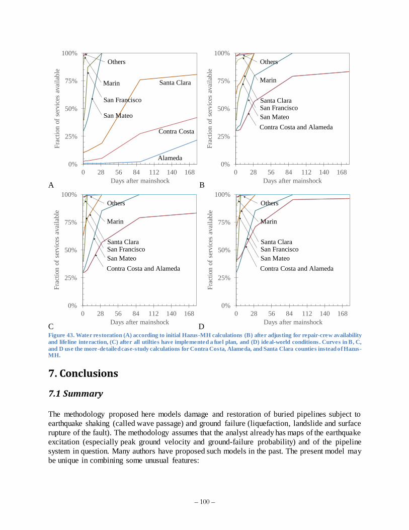
– 100 –
A B
C D Figure 43. Water restoration (A) according to initial Hazus-MH calculations (B) after adjusting for repair-crew availability
and lifeline interaction, (C) after all utilties have implemented a fuel plan, and (D) ideal-world conditions. Curves in B, C,
and D use the more-detailed case-study calculations for Contra Costa, Alameda, and Santa Clara counties instead of Hazus-MH.
7. Conclusions
7.1 Summary
The methodology proposed here models damage and restoration of buried pipelines subject to
earthquake shaking (called wave passage) and ground failure (liquefaction, landslide and surface
rupture of the fault). The methodology assumes that the analyst already has maps of the earthquake
excitation (especially peak ground velocity and ground-failure probability) and of the pipeline
system in question. Many authors have proposed such models in the past. The present model may
be unique in combining some unusual features:
0%
25%
50%
75%
100%
0 28 56 84 112 140 168
Fra
ctio
n o
f se
rvic
es a
vai
lab
le
Days after mainshock
Contra Costa
San Mateo
San Francisco
Santa ClaraMarin
Others
Alameda0%
25%
50%
75%
100%
0 28 56 84 112 140 168
Fra
ctio
n o
f se
rvic
es a
vai
lab
le
Days after mainshock
Contra Costa and Alameda
San Mateo
San FranciscoSanta Clara
Marin
Others
0%
25%
50%
75%
100%
0 28 56 84 112 140 168
Fra
ctio
n o
f se
rvic
es a
vai
lab
le
Days after mainshock
Contra Costa and Alameda
San Mateo
San FranciscoSanta Clara
Marin
Others
0%
25%
50%
75%
100%
0 28 56 84 112 140 168
Fra
ctio
n o
f se
rvic
es a
vai
lab
le
Days after mainshock
Contra Costa and Alameda
San Mateo
San FranciscoSanta Clara
Marin
Others

– 101 –
(1) It treats lifeline interaction and limited consumables by reducing the speed with which
repairs are completed in relation to how important those upstream lifelines and other
resources are to repair productivity. In the example of San Jose Water Company, it was
estimated that lifeline interaction and limited consumables increase the loss of resilience
(measured in terms of lost service-days) by 25 percent.
(2) The model treats aftershocks.
(3) It can be evaluated either deterministically (with no uncertainty) or as stochastic model
(accounting for major sources of uncertainty).
(4) It can be carried out with a GIS system and a spreadsheet and does not require other special
software such as Hazus-MH. Doing so provides the analyst more insight into the
reasonableness of model results and underlying sources of damage and restoration delay.
(5) It offers an approximate method to modify Hazus-MH lifeline damage and restoration-
time estimates to account for lifeline interaction.
(6) It does not require hydraulic analysis of the damaged system or the system as repairs
proceed. That simplification necessarily involves a common but questionable assumption
relating break rate to loss of service, and it prevents the analyst from gaining important
insight into
(7) It mostly avoids reliance on expert opinion and unpublished data. Expert opinion seems to
be required to quantify the rate-limiting factors u and the service time series g(t) for
damage to other lifelines that have not been modeled.
The methodology is applied here to examine the effect of a large hypothetical but not exceedingly
rare earthquake in the San Francisco Bay Area on the buried pipeline network of the San Jose
Water Company and East Bay Municipal Utility District. Results tend to agree with operator
judgment, various restoration measures observed in past earthquakes, and comparable aspects of
other models.
Like all other aspects of any earthquake scenario, the outcomes presented here will invariably
differ in quantity, spatial distribution, and over time from whatever actually happens when (not if)
a large earthquake happens next on the Hayward Fault or other Bay Area fault. By preparing for
the water-supply impacts of this hypothetical earthquake sequence, the reader can be better
prepared for whatever real earthquake actually occurs.
7.2 Research needs
The methodology proposed here mostly avoids reliance on opinion and judgment, but it would be
practical to eliminate reliance on much of what remains. Presumably the u-factors based on expert
opinion could be replaced by compiling sufficient earthquake experience from utilities, perhaps
by some survey analogous to that of Lund and Schiff (1991). The time series g(t) could be replaced
by explicit modeling. It would be interesting to know if there were some theoretical justification
for service restoration following a power law as in Equation (30), and whether or why the power
should be approximately 2/3. It would be also desirable:
To examine more closely or replace the Hazus-MH formulation of the serviceability index.
Can one relate break rate to the fraction of customers receiving various thresholds of flow,
such as minimal flows for cooking and basic sanitary needs?

– 102 –
To know whether and how a large mainshock degrades the seismic resistance of apparently undamaged pipe;
To add treatment of earthquake damage to other elements in the water-supply system,
including tanks, tunnels, canals, valves, and reservoirs;
Regarding the Lund and Schiff (1991) database, it would be desirable for water utilities to adopt a standard database for recording leaks and breaks, especially in earthquakes, so as
to inform future improvements in pipe fragility functions; and
To model the damage to Napa-area water supply systems subjected to the August 24, 2014
South Napa earthquake to see how well it agrees with experience.
8. References cited
Aagaard, B.T., R.W. Graves, D.P. Schwartz, D.A. Ponce, and R.W. Graymer, 2010. Ground-
motion modeling of Hayward Fault scenario earthquakes, part I: construction of the suite of
scenarios. Bulletin of the Seismological Society of America, 100 (6) 2927–2944
Aagaard, B.T., R.W. Graves, A. Rodgers, T.M. Brocher, R.W. Simpson, D. Dreger, N.A.
Petersson, S.C. Larsen, S. Ma, and R.C. Jachens, 2010. Ground-motion modeling of Hayward
Fault scenario earthquakes, part II: simulation of long-period and broadband ground motions.
Bulletin of the Seismological Society of America, 100 (6) 2945–2977
American Water Works Association, 2008. AWWA Small Systems Pipe Repair Checklist, as
published in July 2008 Opflow Question of the Month. 7 pp.
Ang, A.H.S. and W.H. Tang, 1975. Probability Concepts in Engineering Planning and Design,
Vol 1—Basic Principles, John Wiley & Sons, New York, 409 pp.
Bruneau, M., S.E. Chang, R.T. Eguchi, G.C. Lee, T.D. O’Rourke, A,M. Reinhorn, M. Shinozuka,
K. Tierney, W.A. Wallace, and D. von Winterfeldt, 2003. A Framework to Quantitatively Assess
and Enhance the Seismic Resilience of Communities, Earthquake Spectra, 19 (4): 733–752
Committee on Gas and Liquid Fuel Lifelines, 1984. Guidelines for the Seismic Design of Oil and
Gas Pipeline Systems. American Society of Civil Engineers, Technical Council on Lifeline
Earthquake Engineering, Reston, VA, 473 pp.
(ATC) Applied Technology Council, 1991. Seismic Vulnerability and Impact of Disruption of
Lifelines in the Conterminous United States (FEMA 224, ATC-25). Federal Emergency
Management Agency, Washington, DC. http://www.fema.gov/plan/prevent/earthquake/pdf/fema-
224.pdf [viewed 6 June 2006]
Ballantyne, D., E. Berg, J. Kennedy, R. Reneau, and D. Wu, 1990. Earthquake Loss Estimation
Modeling of Seattle Water System, Kennedy/Jenks Inc., Seattle WA, Report to USGS, Grant No.
14-08-000 I-G 1526.

– 103 –
Ballantyne, D., and C. Crouse, 1997. Reliability and Restoration of Water Supply Systems for Fire
Suppression and Drinking Following Earthquakes, prepared for National Institute of Standards
and Technology, NIST GCR 97-730
Benjamin J.R. and C.A. Cornell, 1970. Probability, Statistics, and Decision for Civil Engineers.
Dover Books on Engineering. 704 pp.
Boore, D.M., J.P. Stewart, E. Seyhan, and G.M. Atkinson, 2014. NGA-West2 equations for
predicting PGA, PGV, and 5% damped PSA for shallow crustal earthquakes. Earthquake Spectra
30 (3), 1057-1085.
Byers, W.G., 2008. The ShakeOut Scenario Supplemental Study: Railway Network. SPA Risk
LLC, Denver CO
(CalWARN) California Water/Wastewater Agency Response Network, 2009. Mutual
Aid/Assistance Operational Plan. https://goo.gl/kyT8qE
(CalWARN) California Water/Wastewater Agency Response Network, No date. CalWARN
Mutual Assistance Activated in Response to Napa Earthquake. http://goo.gl/ldZ4jl
Bay City News, 2015. EBMUD Reports 9 Broken Water Pipes Following Quake. August 18, 2015.
http://abc7news.com/news/ebmud-reports-9-broken-water-pipes-following-quake/943303/
[accessed 27 Dec 2015]
Chen W.F. and C.R. Scawthorn, 2003. Earthquake Engineering Handbook, CRC Press, New York,
NY
Contra Costa Local Agency Formation Commission, 2008. Section 9.0, East Bay Municipal Utility
District Water And Wastewater Service, In West Contra Costa County Water and Wastewater
MSR Adopted 8/13/08, Martinez, CA.
http://www.contracostalafco.org/municipal_service_reviews.htm [accessed 26 Oct 2015]
East Bay Municipal Utility District, 2014. Napa’s neighbors to the rescue. Customer Pipeline.
Nov-Dec 2014, p. 1, https://www.ebmud.com/files/1314/3197/7857/customer-pipeline_0.pdf
[accessed 17 Oct 2015]
Eidinger, J., 2001. Seismic Fragility Formulations for Water Systems. American Lifelines
Alliance, G&E Engineering Systems Inc.,
www.americanlifelinesalliance.com/pdf/Part_1_Guideline.pdf, 96 pp.
Field, E.H., Biasi, G.P., Bird, P., Dawson, T.E., Felzer, K.R., Jackson, D.D., Johnson, K.M.,
Jordan, T.H., Madden, C., Michael, A.J., Milner, K.R., Page, M.T., Parsons, T., Powers, P.M.,
Shaw, B.E., Thatcher, W.R., Weldon, R.J., II, and Zeng, Y., 2013. Uniform California earthquake
rupture forecast, version 3 (UCERF3)—The time-independent model: U.S. Geological Survey
Open-File Report 2013–1165, 97 p., California Geological Survey Special Report 228, and
Southern California Earthquake Center Publication 1792, http://pubs.usgs.gov/of/2013/1165/.

– 104 –
Goodson, A., ND. Quantifying and Managing Mutual Aid. East Bay Municipal Utili ty District,
Oakland CA, 38 pp,
http://www.orwarn.org/files/Qualifying%20and%20Managing%20Mutual%20Aid.pdf [accessed
20 Oct 2015]
Heubach, W.F., 1995. Seismic damage estimation for buried pipeline systems. Proc., 4th U.S.
Conference on Lifeline Earthquake Engineering, 312-319.
Honegger D.G. and Eguchi R.T., 1992. Determination of Relative Vulnerabilities to Seismic
Damage for San Diego County Water Authority (SDCWA) Water Transmission Pipelines, October
1992.
Howard, R.A., 1990. From influence to relevance to knowledge. In R.M. Oliver and J.Q. Smith,
eds., Influence Diagrams, Belief Nets and Decision Analysis, New York: John Wiley & Sons, pp.
3-23
Hudnut, K.W., Brocher, T.M., Prentice, C.S., Boatwright, J., Brooks, B.A., Aagaard, B.T., Blair,
J.L., Fletcher, J.B., Erdem, J.E., Wicks, C.W., Murray, J.R., Pollitz, F.F., Langbein, J., Svarc, J.,
Schwartz, D.P., Ponti, D.J., Hecker, S., DeLong, S., Rosa, C., Jones, B., Lamb, R., Rosinski, A.,
McCrink, T.P., Dawson, T.E., Seitz, G., Rubin, R.S., Glennie, C., Hauser, D., Ericksen, T.,
Mardock, D., Hoirup, D.F., and Bray, J.D., 2014. Key Recovery Factors for the August 24, 2014,
South Napa Earthquake: U.S. Geological Survey Open-File Report 2014–1249, 51 p.,
http://dx.doi.org/10.3133/ofr20141249.
Hwang, H., Lin, H., and Shinozuka, M. (1998). “Seismic Performance Assessment of Water
Delivery Systems.” J. Infrastruct. Syst., 4(3), 118–125.
Isoyama, R., and Katayama, T. (1982). Reliability Evaluation of Water Supply Systems During
Earthquakes. Report of the Institute of Industrial Science, the University of Tokyo, 30 (1), 1-64
Javanbarg, M., and C. Scawthorn, 2012. UILLIS: Urban Infrastructure and Lifelines Interactions of
Systems. Proc, 15th World Conference on Earthquake Engineering, September 2012, Lisbon
Portugal
Jayaram, N., and J. Baker, 2009. Correlation model for spatially distributed ground-motion
intensities. Earthquake Engineering and Structural Dynamics 38:1687-1708.
Jeon, S.S. and T.D. O’Rourke, 2005. Northridge earthquake effects on pipelines and residential
buildings. Bulletin of the Seismological Society of America, 95 (1), 294-318
Jones, M.C., 2009. Kumaraswamy’s distribution: a beta-type distribution with some tractability
advantages. Statistical Methodology, 6: 70-81
Kennedy, R.P., Chow, A.W., and Williamson, R.A., 1977. Fault movement effects on buried oil
pipeline, J. Transport. Eng. Div., 103 (TE5), 617–633.

– 105 –
Khater, M., and M. Grigoriu, 1989. Graphical demonstration of serviceability analysis. Structural
Safety and Reliability. ASCE, pp 525-532t
Kuramaswamy, P., 1980. A generalized probability density function for double-bounded random
processes. Journal of Hydrology, 46: 79-88
LADWP, 2014. Westwood / Sunset Trunk Line Repair Update. Press release Sunday August 3,
2014. http://www.ladwpnews.com/go/doc/1475/2218222/
Lilliefors, H., 1967. On the Kolmogorov-Smirnov Test for Normality with Mean and Variance
Unknown, Journal of the American Statistical Association, 62 (318). (June 1967), 399-402
Lund, L. and A. Schiff, 1991. TCLEE Pipeline Failure Database, Technical Council on Lifeline
Earthquake Engineering, American Society of Civil Engineers, Reston, VA, 36 pp.
Lund, L. and C. Davis, 2005. Multihazard mitigation Los Angeles water system: A historical
perspective. In C. Taylor and E. VanMarcke, eds., Infrastructure Risk Management Processes:
Natural, Accidental, and Deliberate Hazards, American Society of Civil Engineers, Reston VA,
224-279.
Lund, L., C.A. Davis, and M.L. Adams, 2005. Water system seismic performance 1994
Northridge-1995 Kobe earthquakes. Proc., Fourth Japan-US Workshop on Seismic Measures for
Water Supply, AWWARF/FWWA, Kobe, Japan, 19-30
Markov I., M. Grigoriu, and T. O'Rourke 1994. An Evaluation of Seismic Serviceability of Water
Supply Networks with Application to San Francisco Auxiliary Water Supply System. NCEER
Report No. 94-0001, National Center for Earthquake Engineering Research, Buffalo NY, 154 pp.
Mid-America Earthquake Center, 2006. MAEviz Software. Urbana, IL: MAE Center, University
of Illinois at Urbana-Champaign.
(NIBS and FEMA) National Institute of Building Sciences and Federal Emergency Management
Agency, 2012. Multi-hazard Loss Estimation Methodology Earthquake Model Hazus®-MH 2.1
Technical Manual. Federal Emergency Management Agency, Washington, DC, 718 pp.
Nojima, N., and H. Kameda, 1991. Cross-impact analysis for lifeline interaction. Proceedings of
the 3rd U.S. Conference on Lifeline Earthquake Engineering, August 22-23, 1991, Los Angeles,
California. American Society of Civil Engineering Technical Council on Lifeline Earthquake
Engineering, pp. 629-638
Ogata, Y., 1998. Space-time point-process models for earthquake occurrences. Annals of the
Institute of Statistical Mathematics, 50 (2): 379-402.
O’Rourke, M.J., 2003. Chapter 23, Buried pipelines. In Chen W.F. and C.R. Scawthorn,
Earthquake Engineering Handbook, CRC Press, New York, NY

– 106 –
O'Rourke M.J., and Ayala G., 1993. Pipeline damage due to wave propagation. Journal of
Geotechnical Engineering, ASCE 119 (9): 1490-1498
O'Rourke, T.D., and M.C. Palmer, 1996. Earthquake performance of gas transmission pipelines.
Earthquake Spectra, 12 (3), 493-527
O’Rourke, T.D., S.S. Jeon, S. Toprak, M. Cubrinovski, M. Hughes, S. van Ballegooy, and D,
Bouziou, 2014. Earthquake response of underground pipeline networks in Christchurch, NZ.
Earthquake Spectra 30 (1) 183–204
O’Rourke, T.D. and Trautmann, C.H., 1980. Analytical Modeling of Buried Pipeline Response to
Permanent Earthquake Displacements, Report No. 80-4, School of Civil Engineering and
Environmental Engineering, Cornell University, Ithaca, NY.
Porter, K.A. C. Scawthorn, D.G. Honegger, T.D. O'Rourke, and F. Blackburn, 1992. Performance
of water supply pipelines in liquefied soil. Proceedings of the 4th US-Japan Workshop on
Earthquake Disaster Prevention for Lifeline Systems, Los Angeles, CA, USA, 08/19-21/91; pp. 3-
17. 1992. http://www.sparisk.com/pubs/Porter-1992-water-pipe-liquefied-soil.pdf [accessed 3 Jul
2015]
Prashar, Y., R. McMullin, B. Cain, and X. Irias, 2012. Pilot Large Diameter Pipeline Seismic
Fragility Assessment. Pipelines Conference 2012, Miami Beach, Florida, August 19-22, 2012,
396-407.
Rose, A., D. Wei, and A. Wein 2011. Economic impacts of the ShakeOut earthquake scenario,
Earthquake Spectra 27, 521-538
San Francisco Bay Area Rapid Transit District, 2015. Remembering Loma Prieta.
http://www.bart.gov/marketing/25-years-after-Loma-Prieta-quake [accessed 27 Dec 2015]
San Francisco Lifelines Council, 2014. Lifelines Interdependency Study 1 Report. San Francisco
Office of the City Administrator, San Francisco, 56 pp.
Scawthorn, C., 1993. Lifeline interaction and post-earthquake functionality. Proceedings of the
5th US-Japan Workshop on Earthquake Disaster Prevention for Lifeline Systems, Tsukuba Science
City, Japan, October 26-27, 1992, 441-450.
Scawthorn, C.R., 2008. The ShakeOut Scenario Supplemental Study: Fire Following Earthquake.
SPA Risk LLC, Denver CO,
http://books.google.com/books?id=mDGrFAw5zqYC&lpg=PA1&dq=shakeout%20fire%20follo
wing&pg=PA1#v=onepage&q&f=false [viewed 26 Oct 2010]
Scawthorn, C., K. Porter, M. Khater, D. Seidel, D. Ballantyne, H.T. Taylor, R.D. Darragh, and C.
Ng, 1992. Utility performance aspects, liquefaction study, Marina and Sullivan Marsh areas, San
Francisco California. National Center for Earthquake Engineering Research, Proceedings from
the 4th Japan-U.S. Workshop on Earthquake Resistant Design of Lifeline Facilities and

– 107 –
Countermeasures for Soil Liquefaction: Tokai University Pacific Center, Honolulu, Hawaii, May
27-29, 1992. Vol. 1., 1992, 317-333. http://www.sparisk.com/pubs/Scawthorn-1992-SF-
Liquefaction-Study.pdf
Schiff, A., 1988. The Whittier Narrows, California earthquake of October 1, 1987—response of
lifelines and their effect on emergency response. Earthquake Spectra 4 (2): 339-366
Seligson, H.A., R.T. Eguchi, L. Lund, and C.E. Taylor, 1991. Survey of 15 Utility Agencies Serving
the Areas Affected by the 1971 San Fernando and 1987 Whittier Narrows Earthquakes . report
prepared for the National Science Foundation. Dames & Moore, Los Angeles CA
Terentieff, S., A. Chen, R. McMullin, Y. Prashar, and X.J. Irias, 2015. Emergency planning and
response damage prediction modeling to mitigate interdependency impacts on water service
restoration. Proc. 9th Water System Seismic Conference, Sendai, Japan October 14-16, 2015.
Tierney, K.J., 1995. Impacts of recent U.S. disasters on businesses: the 1993 Midwest floods and
the 1994 Northridge earthquake. Proc. National Center for Earthquake Engineering Research
Conference on the Economic Impacts of Catastrophic Earthquakes--Anticipating the Unexpected,
New York NY, September 12 and 13, 1995. 52 pp.
Treiman, J., and D. Ponti, 2011. Estimating surface faulting impacts from the ShakeOut scenario
earthquake. Earthquake Spectra, 27 (2) 315–330
Winnipeg City, 2014. Water Main Breaks Frequent Asked Questions (FAQs).
http://www.winnipeg.ca/waterandwaste/water/mainbreaks.stm [last accessed 6 Oct 2015]