Computer Networks 57 (2013) 2536–2548

Contents lists available at SciVerse ScienceDirect

Computer Networks

journal homepage: www.elsevier .com/locate /comnet

DACCER: Distributed Assessment of the Closeness CEntralityRanking in complex networks

1389-1286/$ - see front matter � 2013 Elsevier B.V. All rights reserved.http://dx.doi.org/10.1016/j.comnet.2013.05.001

⇑ Corresponding author. Tel.: +55 24 22336199.E-mail address: ziviani@lncc.br (A. Ziviani).

Klaus Wehmuth, Artur Ziviani ⇑National Laboratory for Scientific Computing (LNCC/MCTI), 25.651-075 Petrópolis, Brazil

a r t i c l e i n f o

Article history:Received 12 September 2012Received in revised form 2 May 2013Accepted 3 May 2013Available online 16 May 2013

Keywords:Network centralityCloseness

a b s t r a c t

We propose a method for the Distributed Assessment of the Closeness CEntrality Ranking(DACCER) in complex networks. DACCER computes centrality based only on localized infor-mation restricted to a limited neighborhood around each node, thus not requiring fullknowledge of the network topology. We indicate that the node centrality ranking com-puted by DACCER is highly correlated with the node ranking based on the traditional close-ness centrality, which requires high computational costs and full knowledge of thenetwork topology by the entity responsible for calculating the centrality. This outcome isquite useful given the vast potential applicability of closeness centrality, which is seldomapplied to large-scale networks due to its high computational costs. Results indicate thatDACCER is simple, yet efficient, in assessing node centrality while allowing a distributedimplementation that contributes to its performance. This also contributes to the practicalapplicability of DACCER to the analysis of large complex networks, as indicated in ourexperimental evaluation using both synthetically generated networks and real-world net-work traces of different kinds and scales.

� 2013 Elsevier B.V. All rights reserved.

1. Introduction

Network centrality is an important tool to analyze com-plex networks [1,2]. In broad terms, network centralitymeasures the relative importance of nodes in a complexnetwork. Different ways of measuring centrality have beenproposed for decades [3–6], each of them suited to assessnode centrality from a different point of view. Examples in-clude using network centrality to evaluate network robust-ness to fragmentation [7,8] or to identify the mostimportant nodes for efficient information spreading in dif-fusion networks [9,10].

As the definitions for centrality vary, so varies the diffi-culty in computing centrality, ranging from low cost (e.g.,degree centrality, where the centrality value of each nodeis its own degree) to others far more costly, such asbetweenness and closeness centralities. The later two, even

though very useful, are costly because they rely on thedetermination of the shortest path between all pairs ofnodes, thus also requiring full knowledge of the networktopology. A high computational cost and the requirementof full knowledge of network topology become significantobstacles for applying the general concept of network cen-trality to the large-scale complex communication net-works we face nowadays [11,12], such as the Internetrouting structure, online social networks, P2P networks,and content distribution networks. Hence, research in net-work science has been recently dedicated to finding newways for dealing with centralities in large-scale networks(Section 5 reviews related work). Typically, these recent ef-forts either (i) optimize the way traditional centralities arecalculated or approximated [13–15]; or (ii) propose meth-ods to distributively assess network centrality withoutrequiring full knowledge of the network topology [8,16].

In particular, we focus on investigating a distributedmethod for approximating the closeness centrality noderanking. The closeness centrality [17] is based on the idea

K. Wehmuth, A. Ziviani / Computer Networks 57 (2013) 2536–2548 2537

that a node is important if it is close to all other nodes inthe network, i.e. the more central a node is the lower its to-tal distance to all other nodes. It is formally defined as

CCðvÞ ¼Xn

i¼1

dðv ; iÞ" #�1

; ð1Þ

where n is the number of nodes on the network and d(v, i)is the distance between nodes v and i.

In general, closeness can be thought of as a measure ofhow fast information spreads from a node to all othernodes in the network. Therefore, closeness centrality isan important traditional measure of centrality that reflectshow efficient information spreading takes place in diffu-sion networks, for instance. Although quite useful in net-work analysis, the computation of the traditionalcloseness centrality is computationally expensive takingO(nm + n2 log n) time [11], where n is the number of nodesand m is the number of edges in the considered network.Such a high computational cost prevents the applicabilityof closeness centrality in large-scale complex networkswe face today.

In this paper, we propose DACCER (Distributed Assess-ment of the Closeness CEntrality Ranking),1 a distributedmethod to assess network centrality based only on localizedinformation restricted to a given neighborhood around eachnode. DACCER computes centrality in a fully distributedway, without requiring full knowledge of the network topol-ogy by the entity responsible for calculating the centrality.

In centrality-based network analysis, the position ofeach node in the centrality ranking is typically moreimportant than the particular centrality value associatedwith each node. As a key contribution, the node centralityranking computed by DACCER is highly correlated with thenode ranking based on the traditional closeness centrality,which requires high computational costs and full knowl-edge of the network topology. This outcome is quite usefulgiven the vast potential applicability of closeness central-ity, which is seldom applied to large-scale networks dueto its high computational costs even if the full networktopology is known [11,12]. We show DACCER is simple,yet efficient, in distributively assessing network centrality.We also indicate that DACCER is best suited to networksthat do not present a highly regular structure, have a smallradius compared to their size, and have low density. Net-works that present small-world or scale-free propertiesin general share such characteristics, making DACCER auseful tool for analyzing such networks that are commonlyfound in practice. This conclusion stems from a thoroughevaluation of DACCER using both synthetically generatednetworks and traces of real-world networks of differentkinds and scales.

This paper proceeds as follows. Section 2 introduces DAC-CER. In Section 3, we present different ways of implementingDACCER. Section 4 analyzes results obtained from applyingDACCER to a diverse set of synthetic and real-world networktraces. We discuss related work in Section 5. Finally, Section 6

1 A shorter preliminary version [18] of this paper appears in theProceedings of the Annual Workshop on Simplifying Complex Networksfor Practitioners (SIMPLEX) at WWW 2012, Lyon, France, April 2012.

concludes the paper and discusses future work. In AppendixA, we present complementary material on DACCER.

2. The DACCER proposal

This section presents the key concepts behind DACCER.

2.1. Neighborhoods

We model a network N as an undirected finite simplegraph G = (V,E), where V is the set of nodes and E the setof edges. The radius r of the network is equivalent to theminimum eccentricity of any node, i.e., r = mini2V(maxj2V

d(i, j)), where d(i, j) is the shortest path distance betweennodes i and j.

We define a neighborhood as an ordered quintuple

Hih ¼ i;h;Vi

h; Eih;/d

� �, where i identifies the central node

of the neighborhood, h is the radius of the neighborhood,

Vih is the set of nodes of V such that their distance to node

i is less or equal to h; Eih is the set of edges in E that are

adjacent to at least one node in Vih, and /d is a function

from Vih to N, such that, for all n 2 Vi

h, /d(n) is the degreeof node n in the original network G.

Note that Vih; E

ih

� �is the induced subgraph of radius h

around the node i. The neighborhood Hih, however, contains

more information than the induced subgraph of radius haround node i. First, the original degrees of all nodes in

Vih—i.e. the degrees of such nodes in the original network

G—are known. Second, contrary to a simple induced sub-graph, the neighborhood definition clearly carries informa-tion about the corresponding central node i and theadopted radius h. Therefore, even if, for instance, h is great-er than the network diameter and all neighborhoods con-tain the same nodes and edges, these neighborhoodswould not be the same; they would be isomorphic. There-fore, given a radius h, each node is actually associated to asingle neighborhood. Moreover, notice that the value re-turned by the function /d(n) in the neighborhood definition

is different of the node degree in Vbh; E

bh

� �when the distance

between the central node and node n is equal to h, i.e. thenode n is located at the border of the neighborhood. Basi-cally, this definition for a neighborhood allows less costly

manipulation of neighborhoods Hih as compared with using

simple induce subgraphs because a subgraph of radius h + 1would be needed to generate the same information.

Fig. 1 illustrates the neighborhoods Hbh for h = {0,1,2}

around the black node b. In Hb0, the set Vb

0 contains onlythe node b, the set Eb

0 is empty and /d(b) = 5, the originaldegree of node b in the original network G. Similarly, inHb

1, the set Vb1 contains node b and its direct neighbors,

while the set Eb1 contains the edges linking a pair of nodes

where both nodes are in Vb1. Note that, in Hb

1, the set Vb1 and

Eb1 thus represent the induced subgraph of radius 1 around

node b. Finally, in the neighborhood Hb2, the set Vb

2 containsnode b, its neighbors, and all the neighbors of its neighbors,while Eb

2 is the set of edges linking nodes of Vb2.

As each node in the network has a unique neighborhoodof radius h defined around itself, we also define the set Hh

Fig. 1. Illustration of neighborhoods Hb0; Hb

1, and Hb2.

2538 K. Wehmuth, A. Ziviani / Computer Networks 57 (2013) 2536–2548

of all neighborhoods of radius h. Notice that, since eachnode i has a unique neighborhood Hi

h; jHhj ¼ jV j.The neighborhoods Hi

h are used to capture localizedinformation from the network that can be used to infer glo-bal features such as the centrality node ranking in the net-work. At a first glance, one can argue that the radius hshould be large enough to make the neighborhoods repre-sentative of the network. Nevertheless, a key reason toavoid large radii is that the cost of determining the neigh-borhoods rises sharply with the increase of the chosen ra-dius. Therefore, the choice of the radius h used todetermine the neighborhoods is crucial for both the effi-ciency and efficacy of DACCER. These trade-offs are evalu-ated in Section 4.

2.2. Classifier function

A classifier is defined as a function fc : Hh ! R, whichassociates a real number to each neighborhood in the setof neighborhoods with radius h. As a consequence, a classi-fier creates a partition in the set of neighborhoods whereeach equivalence class is the set of neighborhoods withthe same value resulting from the classifier. These equiva-lence classes give the centrality ranking shown by DACCER.

At this point, we need to show that there are indeedclassifier functions which can produce a meaningful noderanking able to reflect a notion of node centrality. For in-stance, consider the function fr : Hh ! R, where fr Hi

h

� �¼

jHihj, i.e. the value assigned to each neighborhood is the

number of nodes in the neighborhood. The ranking in-duced in the set of nodes by this classifier coincides exactlywith the ranking obtained by reach centrality [19,20], inwhich the centrality value given to each node is the num-ber of nodes that can be reached in a given number of hopsfrom it. Another example is a classifier that returns for eachnode with neighborhoods of radius h = 1 the classicbetweenness centrality, defined for a node v as CBðvÞ ¼P

i–j2V gijðvÞ=gij, where gij is the number of shortest pathsbetween nodes i and j, while gij(v) is the number of shortest

paths between nodes i and j that pass through node v. Thisarrangement of classifier and radius generates the ego-betweenness centrality defined by Everett and Borgatti[21]. In the following section, we will discuss a volume-based classifier, which generates the traditional degreecentrality [17] when used on neighborhoods with h = 0,and extends its concepts for neighborhoods with radiush > 0, where it generates a centrality ranking highly corre-lated to the ranking obtained by the traditional closenesscentrality [17].

2.3. Volume-based classifier function

In DACCER, we propose the use of a classifier function

fv : Hh ! R, where fv Hih

� �¼ Vol Hi

h

� �. We define the vol-

ume Vol Hih

� �of a neighborhood Hi

h as the sum of the de-

grees of the nodes within it, i.e.

Vol Hih

� �¼Xj2Hi

h

/dðjÞ; ð2Þ

where /d(j) is the degree of node j in the original networkG. For instance, in Fig. 1, the neighborhood Hb

2 of the black

node b has jHb2j ¼ 14 nodes and Vol Hb

2

� �¼ 54, while Hb

1 has

jHb1j ¼ 6 nodes and Vol Hb

1

� �¼ 23, and Hb

0 has jHb0j ¼ 1

nodes and Vol Hb0

� �¼ 5. Clearly, Hi

hþ1 � Hih and

Vol Hihþ1

� �P Vol Hi

h

� �.

To analyze the behavior of this volume-based classifier,first consider the case where the radius used for determin-ing the neighborhoods is h = 0. If h = 0, the volume-basedclassifier generates a centrality notion that coincides withthe classic degree centrality. As h increases, the neighbor-hoods with higher volume intuitively tend to have morenodes in a radius of h + 1. From this, we can argue thatthe neighborhoods with higher volume tend to be the onesin which the central node has the least mean distance to allthe other nodes in the neighborhood. Therefore, as h in-creases, we can expect the centrality ranking generatedby the volume-based classifier to become more correlatedto the node ranking generated by the classic closeness cen-trality [17].

The intuition behind expecting the node ranking basedon the localized volume-based classifier to be correlated tothe node ranking based on the classic closeness centralityresides in the following. Given a neighborhood Hi

h with alarge volume, a relatively low mean distance from node ito all other nodes is expected in that neighborhood. As aconsequence, the resulting node ranking based on adecreasing order of the localized volume of each neighbor-hood with a given h is expected to correlate well with thecloseness centrality node ranking, which is based on anincreasing order of the mean distance between pairs ofnodes. In Section 4, we present experimental results thatsupport this intuition.

K. Wehmuth, A. Ziviani / Computer Networks 57 (2013) 2536–2548 2539

3. DACCER implementation

This section discusses how DACCER can be imple-mented in a fully distributed way as well as in sharedmemory environments for offline analysis. We also presenthow DACCER allows for the distributed location of localand global centrality maxima in the network without fullknowledge of the network topology. In order to discusshow DACCER can be implemented as well as to illustratehow it operates, we use some basic building blocks thatare indeed classic distributed algorithm primitives (orminor variants of them). We explain the operation of thesebasic building blocks to make the DACCER proposal self-contained and accessible to a broad audience.

3.1. Fully distributed DACCER

In this context, we make the following assumptions:

1. Each node in the network knows its direct neighborsand can exchange messages with them; and

2. Each node can run the processes needed for DACCER.

From these assumptions, it should be clear that the kindof networks we refer to in this section are computationalnetworks, such as router networks in the Internet, sensornetworks, wireless ad hoc networks, and other such net-works for which the proposed assumptions hold.

For the DACCER centrality values to be computed for allnodes in the network given a h radius for the neighbor-hoods, each node must take two basic steps:

� to determine its own radius h neighborhood; and� to run the volume-based classifier to get its DACCER

value.

These two steps that start up DACCER are carried out ateach node by the two parallel processes. In doing so, eachnode is actually evaluating the classifier for the neighbor-hood in which it is the central node and then assigning itas the node’s centrality value.

To determine its own neighborhood, in a similar way toa localized broadcast scheme, each node sends its identityand degree to each of its neighbors in a message with time-to-live (TTL) equal to h. This message also carries a uniquemessage id (e.g., the source node id plus a time stamp) inorder to prevent retransmissions of repeated messages.Upon receiving such a message, each node checks the mes-sage id to determine if it has already received this message.If the message is new, the node stores the provided infor-mation—since it is necessary for determining its ownneighborhood. Then, if the message is new and TTL – 0 orthe TTL is larger than the TTL received with this same mes-sage before, the node relays the message to all its neigh-bors with decremented TTL; otherwise, no further actionis taken. As only localized information is required, buffercomplexity of this algorithm at each node i is limited toO jHi

hj� �

. This runs in parallel at each node and after h steps,all nodes know their neighborhoods as required.

We analyze the message complexity Mh of this algo-rithm for a given h value in the following. Each node sendsa message to all its neighbors, then each one of these relaysthis message only once to all its own neighbors, and so onin a process limited by the TTL, which is initially set to h.Therefore, the message from each node i is relayed by allnodes within a radius of h � 1 hops from node i. Hence,the total number of messages used to spread the informa-tion from a given node i is equal to the volume of theneighborhood of radius h � 1 around this node i. In otherwords, the number of messages Mi

h generated by a givennode i using a radius of h hops is

Mih ¼ Vol Hi

h�1

� �¼X

j2Hih�1

/dðjÞ; ð3Þ

where /d(j) is the degree of the node j in the original net-work G. Notice that the mean degree of a neighborhood Hi

h

is given by

dmih ¼ Vol Hi

h

� �=jHi

hj; ð4Þ

where jHihj is the number of nodes within the neighbor-

hood around node i with radius h. Therefore, the numberof messages needed to determine a neighborhood can alsobe written as

Mih ¼ jH

ih�1j � dmi

h�1: ð5Þ

As a consequence, the total number of messages Mh neededto determine the neighborhoods of all nodes in a given net-work N (graph G) can be found by simply summing the re-sult of (3) for all the nodes in the network, leading to

Mh ¼Xi2G

Mih ¼

Xi2G

Xj2Hi

h�1

/dðjÞ; ð6Þ

which, due to (5), can also be written as

Mh ¼Xi2G

Mih ¼

Xi2G

jHih�1j � dmi

h�1

� �: ð7Þ

Even though (6) or (7) account for all messages needed todetermine all neighborhoods within the network, they donot provide a clear insight on how this number of mes-sages varies under changes in the network size, networkdensity, and radius h. A way to achieve an expression thatyields a better insight on this issue is by simplifying theexpression replacing the degree of each node /d(j) with aconstant number. One immediate candidate for this sim-plification is to replace /d(j) with the mean degree dm ofthe network. The motivation for this choice is not basedin considering the mean degree as a good representativeof the degree distribution in the network because in manycases this would typically not be true (e.g., in scale-freenetworks). The motivation actually stems from the factthat as shown by 4, 5 and 7, there is a direct relation be-tween the number of messages needed to determine eachneighborhood and the mean degree of the sub-neighbor-hood of radius h � 1. This is an indication that the messagecomplexity actually depends on the density of each neigh-borhood and by extent on the density of the whole net-work. Further, the use of the mean degree as arepresentative of each node’s degree preserves both the

2540 K. Wehmuth, A. Ziviani / Computer Networks 57 (2013) 2536–2548

density and the volume obtained using the original de-grees; hence, the choice of this value.

After performing such a substitution in (3), the numberof messages Mi

h generated by a given node i using a radiusof h hops can be approximated as

Mih �

Xj2Hi

h�1

dm ¼ jHih�1j � dm; ð8Þ

where dm is the mean degree in the network and jHih�1j is

the number of nodes in the neighborhood of radius h � 1around node i. Thus, we have

jHih�1j ¼ O dh�1

m

� �; ð9Þ

where dh�1m represents the mean degree (dm) raised to the

power h � 1. The proof of this is presented in Proposition1 (see Appendix A). From (8) and (9), we then have that

Mih ¼ O dh

m

� �; ð10Þ

and therefore from (6) we finally have

Mh ¼ O n� dhm

� �; ð11Þ

where n is the number of nodes in the network, dm is themean degree of the network and h is the radius used todetermine the neighborhoods around each node.

From (11), we can have a more insightful view on howthe number of messages is affected by the involved param-eters. The number of messages depends linearly on thenumber of nodes in the network, polynomially on themean degree (which can also be seen as a representationof the network density), and finally it depends exponen-tially on the radius h used to determine the neighborhoodsof each node.

There is still a further insight on the message com-plexity Mh to determine the neighborhoods that is noteasily perceived from (11). When considering the depen-dence of the number of messages on the radius h, sincethe messages are not forwarded arbitrarily, we shouldrealize that for finite networks the number of messagesneeded to determine the neighborhoods is bounded,regardless of h. To see that, consider a value of h suchthat h = D(G), where D(G) is the network diameter. Sincewe are supposing the network G to be finite, so is D(G).In this case, the neighborhoods of every node in the net-work are isomorphic and contain the whole network.This is because, given an arbitrary node i, any othernode in the network can be reached in no more thanD(G) hops. Therefore, the number of messages in thiscase is

MDðGÞ ¼ n� VolðGÞ ¼ 2� n�m; ð12Þ

where m is the number of edges and the other parametersare already defined. Since there cannot be any neighbor-hood larger than the whole network, we observe that mak-ing h > D(G) does not increase the number of messages andso the number of messages needed to determine the neigh-borhoods on any given (finite) network has an upperbound of 2 � n �m.

As for the time complexity of the fully distributedimplementation of DACCER, the message of each node

has to spread for h hops to reach all its destinations. Sincethe messages generated by each node do not interfere withthe messages of any other node, they can all be handledsimultaneously, meaning that all neighborhoods can bedetermined in h time steps. Therefore, the time complexityof DACCER is

Th ¼ OðhÞ: ð13Þ

Note that to compute the exact closeness centrality values,the computation of All-Pairs Shortest Paths (APSPs) is re-quired. Holzer and Wattenhofer [22] have recently pro-posed a distributed algorithm to compute APSP in O(n)time. For practical purposes, considering networks withsmall-world and scale-free properties as the ones targetedby DACCER, the network radius is typically much smallerthan the number of nodes n in the network. As a conse-quence, the time complexity of DACCER presented in (13)is much smaller than the result achieved by [22] for com-puting APSP in a distributed way, i.e., O(h)� O(n). Indeed,we indicate later in the paper that h as low as 2 is a suitablechoice to balance the trade-off between achieving a lowcost and a high correlation between rankings provided bycloseness centrality and DACCER (see Section 4.2).

After each node i has determined its Hih neighborhood,

the centrality values for all nodes can be calculated. Forthat, each node i runs DACCER’s classifier, which calculates

Vol Hih

� �. Furthermore, each localized volume Vol Hi

h

� �con-

sists of a simple sum of jHihj terms, therefore having a linear

computational cost of O jHihj

� �for each node.

3.2. DACCER in shared memory environments

In this section, we present another possible implemen-tation of DACCER, aimed for application in networks whosetopology is fully known at a specific entity. The goal of thissection is to show that DACCER is also applicable for thisclass of problems. The main concepts of the method arethe same, but for this implementation of DACCER the fol-lowing assumptions are considered:

1. The network topology is fully known by a specificentity; and

2. can be represented in a shared memory environment.

The main idea behind this implementation of DACCER isto build the neighborhood of each node in memory andthen run the classifier to determine its centrality value.One possible implementation is to use a set structure tostore the neighborhood and an auxiliary list to hold anexpanding fringe that represents the nodes that potentiallyhave neighbors not yet included in the set of neighbor-hood. The set structure is used to avoid the existence ofduplicated nodes in the neighborhood. In this implementa-tion, we consider that such a set structure is implementedby a binary balanced tree, such as a red–black tree [24].The neighborhood determination algorithm starts withthis set and also the fringe list containing the central nodei of the considered neighborhood. At this point, if h = 0, weare done; otherwise, the algorithm attempts to insert all

K. Wehmuth, A. Ziviani / Computer Networks 57 (2013) 2536–2548 2541

neighbors from all nodes in the fringe list into the neigh-borhood set. Every time this insertion succeeds, the samenode is inserted onto a new fringe list. When all nodes inthe current fringe list are processed, this list is discardedand replaced by the new constructed list. Then a new cycleis run, until the configured h radius is achieved. This proce-dure is shown in Algorithm 1.

Algorithm 1. getNeighborhoodði; hÞ

1: neighborhoodSet i2: fringeList i3: c 04: while c < h do5: auxList empty6: for all n 2 fringeList do7: for all p is neighbor of n do8: neighborhoodSet p9: if insert succesful then10: auxList p11: end if12: end for13: end for14: fringeList empty15: fringeList auxList16: end while17: return neighborhoodSet

In order to determine the time complexity of Algorithm1, we consider that each node in a neighborhood of radiush � 1 attempts to insert all its neighbors into the set struc-

ture, meaning that there are Vol Hih�1

� �insertion attempts

to the set structure. We consider the time complexity ofeach insertion to be O(1), which can be achieved using acoloring scheme similar to those commonly used in aBreadth-first search (BFS) algorithm [24] or a Bloom filter[25,26]. Repeating the reasoning from (3)–(10) in Sec-

tion 3.1, the time complexity Tih to determine the neighbor-

hood of node i is

Tih ¼ O dh

m

� �; ð14Þ

where dm is the network mean degree and h the neighbor-hood radius. From this, since the neighborhoods of allnodes in the network have to be determined, the overalltime complexity Th for the neighborhood determination is

Th ¼ O n� dhm

� �; ð15Þ

where n is the number of nodes on the network, dm is thenetwork mean degree and h the neighborhood radius.

We remark DACCER is best suited to be applied tosparse networks, thus having a low mean degree. Further,as shown empirically in Section 4, DACCER can be effi-ciently applied using low values for the neighborhood ra-dius h. As a consequence, dh

m is typically much smallerthan the number of edges m of the analyzed large-scalenetworks, thereby making DACCER considerably fasterthan the traditional algorithm for closeness centrality,

which relies on the All Pairs Shortest Path (APSP) algorithmwith time complexity O(nm).

After each neighborhood has been determined, the cen-trality value for each node can be computed using thesame volume-based classifier described in Section 2.3.

Since each neighborhood can be determined indepen-dently of all others, this process is very well suited for aparallel implementation to speed up processing. In Sec-tion 4.4, we present experimental evidence supporting thisclaim.

4. Performance evaluation

In this section, we present experimental resultsconcerning:

� the comparison of node rankings provided by DACCER,closeness centrality, and degree centrality (Section 4.1);� the trade-off between neighborhood size and applica-

bility costs (Section 4.2);� the trade-off between neighborhood size and the

achieved correlation of DACCER with the closeness cen-trality ranking (Section 4.3);� the practical applicability of DACCER in large-scale net-

works (Section 4.4).

4.1. Correlation between DACCER and closeness centrality

At the end of Section 3.1, we argue that we expect ahigh correlation between the node rankings provided bycloseness centrality and DACCER. In this section, we exper-imentally confirm this claim by analyzing the correlationbetween these rankings obtained for different syntheti-cally generated networks as well as traces of real-worldnetworks. Since it is known that degree centrality mayhave a fairly high correlation to closeness centrality[27,23], we also compare the node ranking correlation ob-tained between DACCER and closeness centrality with thenode ranking correlation obtained between degree andcloseness centralities. Notice that the node ranking ob-tained by degree centrality is the same obtained by DAC-CER when using h = 0 for determining the neighborhoodsof each node.

We first evaluate the correlation obtained in two kindsof synthetic networks: 100 scale-free networks based onthe Barabási-Albert (BA) model [28] and 100 random net-works based on the Erdös-Rényi (ER) model [29]. The BAnetworks have 1000 nodes each and are created with 5connections per new node, resulting in a 9.95 mean nodedegree. The ER networks also have 1000 nodes and a con-nection probability p = 0.01, which corresponds to1:5� ln 1000

1000 , ensuring that the resulting networks are con-nected as it is known that p > ln n

n is a sharp threshold forthe connectedness of ER networks [30]. The mean degreeof the ER networks can vary, but in this case remains closeto 10.

Fig. 2 shows the correlation between the rankings pro-vided by DACCER and by closeness centrality for each nodein one BA and one ER network, both randomly chosenamong the set of 100 BA and 100 ER networks. At the left

0

100

200

300

400

500

600

700

800

900

1000

0 100 200 300 400 500 600 700 800 900 1000

Clo

sene

ss c

entra

lity

node

rank

ing

DACCER (h=2) node ranking

R = 0.9979

0

100

200

300

400

500

600

700

800

900

1000

0 100 200 300 400 500 600 700 800 900 1000

Clo

sene

ss c

entra

lity

node

rank

ing

Degree centrality node ranking

R = 0.6443

0

100

200

300

400

500

600

700

800

900

1000

0 100 200 300 400 500 600 700 800 900 1000

Clo

sene

ss c

entra

lity

node

rank

ing

DACCER (h=2) node ranking

R = 0.9970

0

100

200

300

400

500

600

700

800

900

1000

0 100 200 300 400 500 600 700 800 900 1000

Clo

sene

ss c

entra

lity

node

rank

ing

Degree centrality node ranking

R = 0.9420

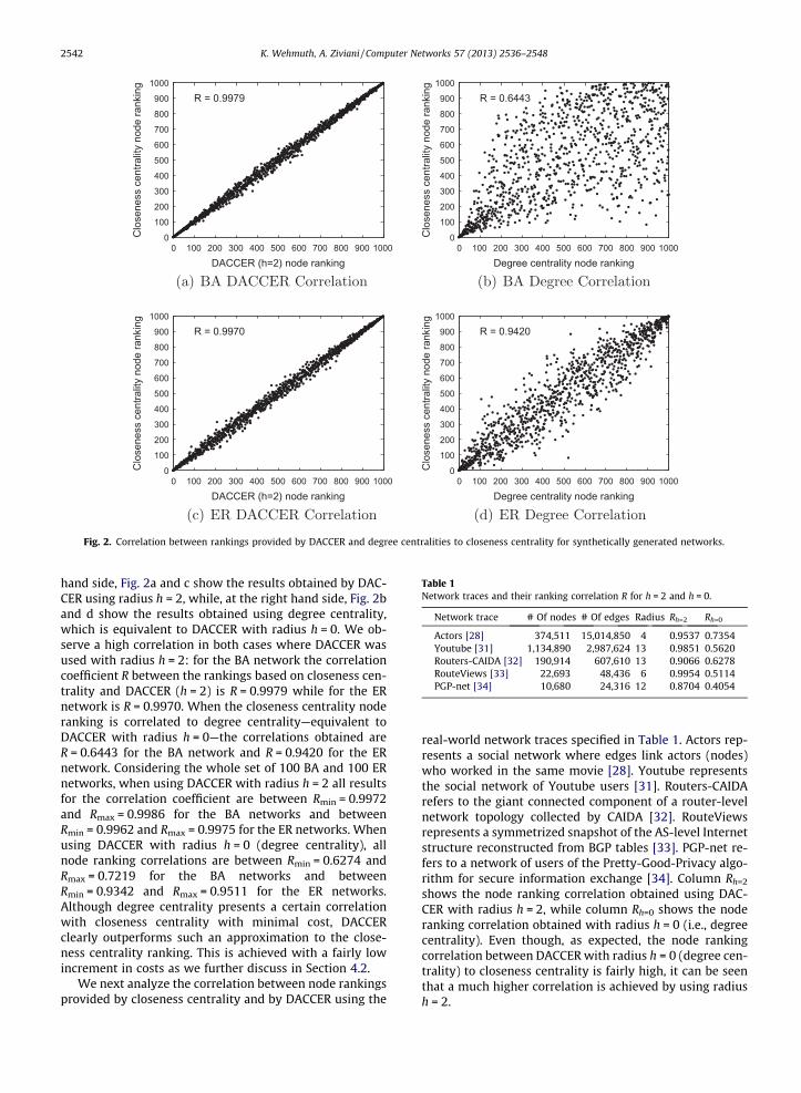
Fig. 2. Correlation between rankings provided by DACCER and degree centralities to closeness centrality for synthetically generated networks.

Table 1Network traces and their ranking correlation R for h = 2 and h = 0.

Network trace # Of nodes # Of edges Radius Rh=2 Rh=0

Actors [28] 374,511 15,014,850 4 0.9537 0.7354Youtube [31] 1,134,890 2,987,624 13 0.9851 0.5620Routers-CAIDA [32] 190,914 607,610 13 0.9066 0.6278RouteViews [33] 22,693 48,436 6 0.9954 0.5114PGP-net [34] 10,680 24,316 12 0.8704 0.4054

2542 K. Wehmuth, A. Ziviani / Computer Networks 57 (2013) 2536–2548

hand side, Fig. 2a and c show the results obtained by DAC-CER using radius h = 2, while, at the right hand side, Fig. 2band d show the results obtained using degree centrality,which is equivalent to DACCER with radius h = 0. We ob-serve a high correlation in both cases where DACCER wasused with radius h = 2: for the BA network the correlationcoefficient R between the rankings based on closeness cen-trality and DACCER (h = 2) is R = 0.9979 while for the ERnetwork is R = 0.9970. When the closeness centrality noderanking is correlated to degree centrality—equivalent toDACCER with radius h = 0—the correlations obtained areR = 0.6443 for the BA network and R = 0.9420 for the ERnetwork. Considering the whole set of 100 BA and 100 ERnetworks, when using DACCER with radius h = 2 all resultsfor the correlation coefficient are between Rmin = 0.9972and Rmax = 0.9986 for the BA networks and betweenRmin = 0.9962 and Rmax = 0.9975 for the ER networks. Whenusing DACCER with radius h = 0 (degree centrality), allnode ranking correlations are between Rmin = 0.6274 andRmax = 0.7219 for the BA networks and betweenRmin = 0.9342 and Rmax = 0.9511 for the ER networks.Although degree centrality presents a certain correlationwith closeness centrality with minimal cost, DACCERclearly outperforms such an approximation to the close-ness centrality ranking. This is achieved with a fairly lowincrement in costs as we further discuss in Section 4.2.

We next analyze the correlation between node rankingsprovided by closeness centrality and by DACCER using the

real-world network traces specified in Table 1. Actors rep-resents a social network where edges link actors (nodes)who worked in the same movie [28]. Youtube representsthe social network of Youtube users [31]. Routers-CAIDArefers to the giant connected component of a router-levelnetwork topology collected by CAIDA [32]. RouteViewsrepresents a symmetrized snapshot of the AS-level Internetstructure reconstructed from BGP tables [33]. PGP-net re-fers to a network of users of the Pretty-Good-Privacy algo-rithm for secure information exchange [34]. Column Rh=2

shows the node ranking correlation obtained using DAC-CER with radius h = 2, while column Rh=0 shows the noderanking correlation obtained with radius h = 0 (i.e., degreecentrality). Even though, as expected, the node rankingcorrelation between DACCER with radius h = 0 (degree cen-trality) to closeness centrality is fairly high, it can be seenthat a much higher correlation is achieved by using radiush = 2.

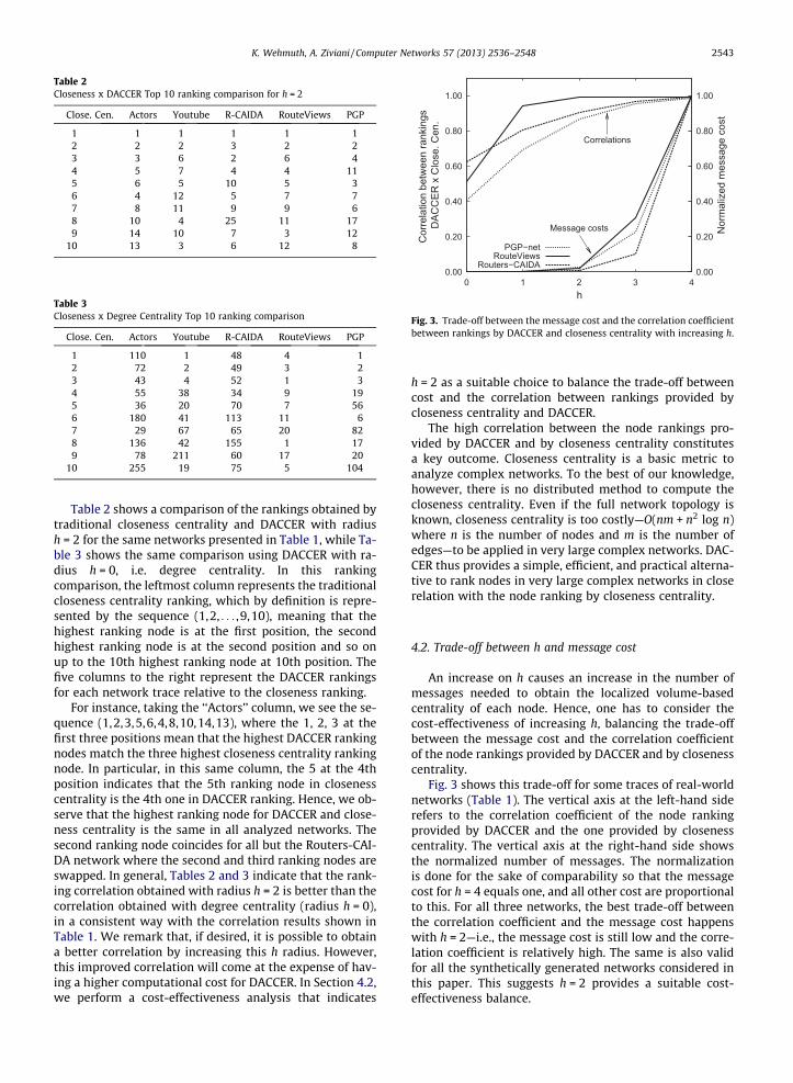
Table 2Closeness x DACCER Top 10 ranking comparison for h = 2

Close. Cen. Actors Youtube R-CAIDA RouteViews PGP

1 1 1 1 1 12 2 2 3 2 23 3 6 2 6 44 5 7 4 4 115 6 5 10 5 36 4 12 5 7 77 8 11 9 9 68 10 4 25 11 179 14 10 7 3 12

10 13 3 6 12 8

Table 3Closeness x Degree Centrality Top 10 ranking comparison

Close. Cen. Actors Youtube R-CAIDA RouteViews PGP

1 110 1 48 4 12 72 2 49 3 23 43 4 52 1 34 55 38 34 9 195 36 20 70 7 566 180 41 113 11 67 29 67 65 20 828 136 42 155 1 179 78 211 60 17 20

10 255 19 75 5 104

0.00

0.20

0.40

0.60

0.80

1.00

0 1 2 3 40.00

0.20

0.40

0.60

0.80

1.00

Cor

rela

tion

betw

een

rank

ings

D

ACC

ER x

Clo

se. C

en.

Nor

mal

ized

mes

sage

cos

t

h

Correlations

Message costs

PGP−netRouteViews

Routers−CAIDA

Fig. 3. Trade-off between the message cost and the correlation coefficientbetween rankings by DACCER and closeness centrality with increasing h.

K. Wehmuth, A. Ziviani / Computer Networks 57 (2013) 2536–2548 2543

Table 2 shows a comparison of the rankings obtained bytraditional closeness centrality and DACCER with radiush = 2 for the same networks presented in Table 1, while Ta-ble 3 shows the same comparison using DACCER with ra-dius h = 0, i.e. degree centrality. In this rankingcomparison, the leftmost column represents the traditionalcloseness centrality ranking, which by definition is repre-sented by the sequence (1,2, . . . ,9,10), meaning that thehighest ranking node is at the first position, the secondhighest ranking node is at the second position and so onup to the 10th highest ranking node at 10th position. Thefive columns to the right represent the DACCER rankingsfor each network trace relative to the closeness ranking.

For instance, taking the ‘‘Actors’’ column, we see the se-quence (1,2,3,5,6,4,8,10,14,13), where the 1, 2, 3 at thefirst three positions mean that the highest DACCER rankingnodes match the three highest closeness centrality rankingnode. In particular, in this same column, the 5 at the 4thposition indicates that the 5th ranking node in closenesscentrality is the 4th one in DACCER ranking. Hence, we ob-serve that the highest ranking node for DACCER and close-ness centrality is the same in all analyzed networks. Thesecond ranking node coincides for all but the Routers-CAI-DA network where the second and third ranking nodes areswapped. In general, Tables 2 and 3 indicate that the rank-ing correlation obtained with radius h = 2 is better than thecorrelation obtained with degree centrality (radius h = 0),in a consistent way with the correlation results shown inTable 1. We remark that, if desired, it is possible to obtaina better correlation by increasing this h radius. However,this improved correlation will come at the expense of hav-ing a higher computational cost for DACCER. In Section 4.2,we perform a cost-effectiveness analysis that indicates

h = 2 as a suitable choice to balance the trade-off betweencost and the correlation between rankings provided bycloseness centrality and DACCER.

The high correlation between the node rankings pro-vided by DACCER and by closeness centrality constitutesa key outcome. Closeness centrality is a basic metric toanalyze complex networks. To the best of our knowledge,however, there is no distributed method to compute thecloseness centrality. Even if the full network topology isknown, closeness centrality is too costly—O(nm + n2 log n)where n is the number of nodes and m is the number ofedges—to be applied in very large complex networks. DAC-CER thus provides a simple, efficient, and practical alterna-tive to rank nodes in very large complex networks in closerelation with the node ranking by closeness centrality.

4.2. Trade-off between h and message cost

An increase on h causes an increase in the number ofmessages needed to obtain the localized volume-basedcentrality of each node. Hence, one has to consider thecost-effectiveness of increasing h, balancing the trade-offbetween the message cost and the correlation coefficientof the node rankings provided by DACCER and by closenesscentrality.

Fig. 3 shows this trade-off for some traces of real-worldnetworks (Table 1). The vertical axis at the left-hand siderefers to the correlation coefficient of the node rankingprovided by DACCER and the one provided by closenesscentrality. The vertical axis at the right-hand side showsthe normalized number of messages. The normalizationis done for the sake of comparability so that the messagecost for h = 4 equals one, and all other cost are proportionalto this. For all three networks, the best trade-off betweenthe correlation coefficient and the message cost happenswith h = 2—i.e., the message cost is still low and the corre-lation coefficient is relatively high. The same is also validfor all the synthetically generated networks considered inthis paper. This suggests h = 2 provides a suitable cost-effectiveness balance.

2544 K. Wehmuth, A. Ziviani / Computer Networks 57 (2013) 2536–2548

4.3. Trade-off between h and closeness correlation

If the radius h used to determine the neighborhoodsreaches the network radius, the neighborhoods with thehighest volume will be the ones associated with the nodeswith smallest eccentricity. For instance, the nodes with thesmallest eccentricity in the network have eccentricityequal to the network radius. Therefore, the neighborhoodscentered on these nodes comprise the whole network, hav-ing the highest possible volume. From this point on, whenh increases surpassing the network radius, the number ofneighborhoods tied at the first place of the DACCER cen-trality ranking also increases, due to the fact that moreneighborhoods become isomorphic. This has the effect ofdecreasing the correlation between the node rankings byDACCER and closeness centrality since the tied neighbor-hoods will force their associated nodes to stay on the sameequivalence class, making them undistinguishable. Thesame behavior also occurs for other equivalence classesthan just the top ranking ones. However, this effect tendsto be more noticeable on high ranking equivalence classes,since they are associated to large high volume neighbor-hoods which do not have much room to grow. We performan experiment using an Erdös–Rényi (ER) network with1454 nodes, 1684 edges, radius 15, and diameter 26. Thisnetwork is conceived to have a relatively large radius ascompared with its size, so we can vary the radius h usedto determine the neighborhoods and observe its impacton the ranking correlation of DACCER and the classic close-ness centrality.

Fig. 4 shows the result obtained from this experiment.The left vertical axis, related to the continuous curve,shows the correlation between the rankings of DACCERand closeness centrality. The right vertical axis, related tothe dashed curve, shows the normalized number of tiesat the first place on the DACCER ranking, i.e. the numberof ties divided by the number of nodes in the network.The horizontal axis shows the radius h used to determinethe neighborhood of each node, varying from 0 to 26.When h = 0, the result obtained by DACCER is equal tothe traditional degree centrality, showing that the correla-tion obtained between degree centrality and closenesscentrality for this network is about 0.5, which is in the

0.00

0.20

0.40

0.60

0.80

1.00

0 5 10 15 20 25

Cor

rela

tion

betw

een

rank

ings

D

ACC

ER x

Clo

se. C

en.

Firs

t pla

ce ti

es ra

tio

h

CorrelationFirst Place Ties

Fig. 4. Behavior of the correlation between rankings by DACCER andcloseness centrality with increasing h.

expected range as shown in [23,27]. At this same point, itcan be seen that the number of first place ties is 0, indicat-ing that this network has only one node with the highestdegree found in the network. Observing the continuouscurve, we see that the correlation grows rapidly as h in-creases from 0 to 5. Based on this, we observe that the bestchoices for h for this network would be in the range of 2–5.At the same range, we observe from the dashed curve thatthere is no significant number of ties for the first rankingplace, as expected. From that point on, the correlation ob-tained stays high and number of ties low up to the pointwhere h reaches a value equal to the network radius(h = 15). From that point on, the number of ties increasesrapidly and the correlation drops sharply, as expected.When h reaches 24, all neighborhoods virtually containall nodes in the network, making them undistinguishablefor DACCER and therefore driving the correlation to virtu-ally zero.

This experiment is also useful to illustrate why DACCERis not well suited for use in networks with highly regularstructures. On such networks there will be a high quantityof isomorphic neighborhoods, causing DACCER to assign allof them to the same equivalence class and therefore caus-ing a high rate of ties, hindering the correlation achieved tocloseness centrality.

4.4. Practical applicability of DACCER

DACCER only requires each node to know the degrees ofthe nodes belonging to its neighborhood. This means DAC-CER can be used in networks where each node only knowsits direct neighbors (Section 3.1) and also in networkswhere the topology is fully known (Section 3.2). Further-more, DACCER can be implemented in different ways,ranging from a centralized approach running on a singleCPU core to a fully distributed approach with the analysisof each node running on a separate core.

To evaluate the practical applicability of DACCER, wecompare the time spent for calculating the closeness cen-trality ranking using the traditional algorithm running ona single CPU core with DACCER implementation describedin Section 3.2, running on 1 and 32 CPU cores, each coreequivalent to the one used for traditional closeness. Inthese experiments, we have used 4 Sun Blade x6250 nodes,each one with a dual quad-core Intel (R) Xeon (R) CPUE5440 (therefore, with a total of eight cores in each node)and 16 GB of RAM memory. This study evaluates the per-formance gains allowed by DACCER, even in a modestlyparallelized implementation, when compared with the tra-ditional implementation of closeness centrality, which isnot easily parallelizable. In the parallelized DACCER imple-mentation, the network nodes are distributed among the32 cores and each core calculates the centrality of its as-signed nodes. The whole network topology information isavailable to all cores in shared memory.

Fig. 5 presents the execution time in seconds to com-pute the closeness centrality ranking and the DACCERranking as a function of the network complexity. As themeasure of network complexity, we consider the numberof nodes n times the number of edges m of each analyzednetwork. Fig. 5a and b show the time spent to compute

102

103

104

105

106

107

108 109 1010 1011 1012 1013Ti

me

(sec

)

network complexity (n x m)

PGP−net

RouteViews

Routers−CAIDA

Actors

100

101

102

103

104

108 109 1010 1011 1012 1013

Tim

e (s

ec)

network complexity (n x m)

PGP−net

RouteViews

Routers−CAIDA

Actors

100

101

102

103

104

1011 1012 1013 1014

Tim

e (s

ec)

network complexity (n x m)

Routers−CAIDA

Youtube

Actors

Skitter−AS

Fig. 5. Execution times for closeness and DACCER node rankings.

K. Wehmuth, A. Ziviani / Computer Networks 57 (2013) 2536–2548 2545

the closeness centrality ranking and the DACCER rankingfor the network traces presented in Table 1 in a singleCPU core, respectively. In turn, in Fig. 5c, we present thetime spent to compute the centrality ranking based onDACCER using 32 CPU cores. Fig. 5c shows results for thethree largest networks in Table 1, namely Routers-CAIDA,Youtube and Actors, and for one additional large network:the Internet Autonomous systems network collected bySkitter [35] with 1,696,415 nodes and 11,095,298 edges.This latter network presents a scale that strongly limitsthe practical applicability of the closeness centrality torank their nodes. We emphasize that Fig. 5a uses a differ-ent scale for the execution time than Fig. 5b and c. For in-stance, the computation of the closeness centrality rankingfor the Actors network takes 3 � 106 s (roughly 34 days) inthe single CPU core, whereas the DACCER centrality rank-ing is computed after 6500 s (about 1.8 h) using the singleCPU core and in only 640 s (about 10 min) using the 32CPU cores. From this experiment, it becomes clear that,even with a modest parallelization, DACCER is orders ofmagnitude faster than the traditional closeness centralityalgorithm. Therefore, the possibility of parallelizing DAC-CER execution makes it applicable to the analysis oflarge-scale networks for which it would be unfeasible inpractice to compute closeness centrality. For instance, theSkitter-AS network is analyzed using DACCER in about1 h using the 32 CPU cores. Further, DACCER does not re-quire full knowledge of the network topology at a specificentity, being therefore applicable on networks where thetopology is not fully known.

5. Related work

There are many centrality measures for assessing therelative importance of different nodes in a network underdifferent criteria, such as its capacity for information

diffusion or its relevance for connectivity. Examples arethe traditional degree, betweenness, closeness, and eigen-vector centralities [3,4].

The computing of most of the traditional centralities isin general computationally expensive and requires fullknowledge of the network topology. Therefore, some re-cent efforts are dedicated to optimize the way by whichtraditional centralities are calculated or approximated[13–15]. These methods, however, still require full knowl-edge of the network topology to compute a centralityapproximation, hindering their applicability to large-scalenetworks where such an information is unavailable and adistributed implementation is required.

Alternatively, as our proposal, some previous worksinvestigate methods to assess network centrality in a dis-tributed way, without requiring full knowledge of the net-work topology. Nanda and Kotz [16] propose a newcentrality metric called Localized Bridging Centrality(LBC), which is targeted at locating bridges, i.e., edgeswhose removal disconnects the network using only one-hop neighborhoods around each node. The proposed useof LBC is on relatively small-scale wireless mesh networks.Lim et al. [23] find the top-k centrality nodes on a networkby sampling. Kermarrec et al. [8] use a random walk to dis-tributively assess network centrality in complex networks,however their random walk approach does not particularlycorrelate with closeness centrality and presents a highconvergence time. In contrast, Alahakoon et al. [36]approximate betweenness centrality with multiple limitedrandom walks.

Marsden [37] indicates empirical evidence that local-ized centrality measures computed for one-hop neighbor-hood are highly correlated to a global centrality measure.Everett and Borgatti [21] as well as Ercsey-Ravasz andToroczkai [38] explore this notion to approximatebetweenness centrality. In a recent paper, Pfeffer andCarley [39] evaluate bounded-distance shortest path

2546 K. Wehmuth, A. Ziviani / Computer Networks 57 (2013) 2536–2548

calculations and their potential to approximate shortestpath centralities, such as betweenness and closeness. Inthis paper, we extend this notion by proposing DACCERand indicating that the node ranking based on its localizedvolume-based centrality correlates quite well with thecloseness centrality ranking.

6. Conclusion

In this paper, we propose DACCER, a novel distributedmethod to approximate the closeness centrality rankingin large complex networks, without requiring full knowl-edge of the network topology. DACCER computes a local-ized volume-based centrality at each node consideringonly a limited neighborhood of h hops around everynode. DACCER also provides a navigation procedureallowing the location of the most central nodes. In short,DACCER achieves a node ranking that is highly correlatedwith the ranking based on the traditional closeness cen-trality, whereas with applicability costs that are signifi-cantly lower. We indicate h = 2 provides a suitabletrade-off between limited message costs and high corre-lation with the closeness centrality ranking. In particular,although degree centrality—equivalent to DACCER withh = 0—presents a certain correlation with closeness cen-trality with minimal cost [27,23], DACCER with h = 2strongly outperforms degree centrality as an approxima-tion to the ranking of closeness centrality while keepingthe associated costs under control. This way, DACCERcan be viewed as an extension of the degree centralityconcept, by applying it to a neighborhood and therebyincreasing the correlation obtained to closeness central-ity. We indicate DACCER is best suited to networks thatdo not present a highly regular structure, have a smallradii compared with their size, and have low density.Many complex networks of interest present these charac-teristics, such as small-world and scale-free networks,thus rendering DACCER applicable to the practical analy-sis of these networks.

It is important to notice that DACCER uses this vol-ume-based classifier function to determine a node rank-ing that approximates the node ranking based oncloseness centrality. Therefore, for DACCER to work prop-erly, the classifier function has to able to discriminatethe neighborhoods based on their volume. It followsfrom this that DACCER will not work properly for net-works in which this is unachievable. To illustrate thiscase, for instance, DACCER is inappropriate to evaluatea regular network, where all neighborhoods have thesame number of nodes and edges (and therefore thesame volume), because the involved neighborhoods can-not be discriminated. Likewise, a line network, which isvery close to be regular since all nodes except two haveexactly two connections, would make DACCER to behavepoorly. We emphasize, however, that although DACCER isunsuited for some kinds of very particular networks asthose mentioned, DACCER is very effective when consid-ering networks that have irregular structure, small radiuscompared with their size, and low density—i.e., have asmall mean degree. In particular these characteristics

are present in many examples of practical networks thatshare small-world or scale-free properties, making themsuitable for DACCER.

Following the encouraging results we found for DAC-CER approximating the closeness centrality ranking, weplan to investigate in our future work other (local) classi-fier functions that may infer different global metrics inlarge-scale complex networks based on localized informa-tion. Furthermore, most complex networks also presentdynamic behavior [40,41]. As future work, we plan toinvestigate how DACCER can contribute to the analysisand modeling of the dynamic behavior of complexnetworks.

Acknowledgment

Authors thank Alan Mislove (Northeastern University)for providing the datasets used in [31]. Authors alsothank Ana Paula C. da Silva (UFJF), Antônio Tadeu A.Gomes (LNCC), Daniel R. Figueiredo (UFRJ), and Éric Fle-ury (ENS-Lyon/INRIA) for their comments on our work.This work was partially supported by the Brazilian Fund-ing Agencies FAPERJ and CNPq, as well as by the Brazil-ian Ministry of Science Technology and Innovation(MCTI).

Appendix A. Complementary material on DACCER

Proposition 1. jHihj ¼ O dh

m

� �.

Proof. We will show that limh!1jHi

h jdh

mis finite. As stated and

analyzed in Section 3.1, we assume that every node hasdegree dm.

First we show that jHihj 6 dh

m þ dh�1m þ . . .þ dm þ 1.

Note that for h ¼ 0; jHi0j ¼ 1, since only i 2 Hi

0. Consideringthat the node i has degree dm; jHi

1j 6 dm þ 1, and furtherthat there are at most dm nodes at distance 1 of node i.Since each node at distance 1 of node i has degree dm, itcan have only less than dm neighbors at distance 2 fromnode i. Since there are at most dm nodes at distance 1 of i,there can be no more than d2

m nodes at distance 2 from i.Consequently, jHi

2j 6 d2m þ dm þ 1. Extending this argu-

ment, we have that jHihj 6 dh

m þ dh�1m þ � � � þ dm þ 1.

We now show that limh!1jHi

h jdh

mis finite:

limh!1

jHihj

dhm

6dh

m

dhm

þ dh�1m

dhm

þ . . .þ dm

dhm

þ 1

dhm

6 1þ 1dmþ 1

d2m

þ . . .þ 1

dh�1m

þ 1

dhm

limh!1

jHihj

dhm

6 1þ 1dmþ 1

dm

� �2

þ . . .þ 1dm

� �h�1

þ 1dm

� �h

: ðA:1Þ

Notice that when h grows arbitrarily, the right hand side of(A.1) converges to the geometric series

K. Wehmuth, A. Ziviani / Computer Networks 57 (2013) 2536–2548 2547

X1h¼0

1dm

� �h

: ðA:2Þ

Since this series is known to be convergent, it follows that

limh!1

jHihj

dhm

< C;

and jHihjis O dh

m

� �. h

References

[1] R. Albert, A. Barabási, Statistical mechanics of complex networks,Reviews of Modern Physics 74 (1) (2002) 47–97.

[2] M.E.J. Newman, The structure and function of complex networks,SIAM Review 45 (2) (2003) 167–256.

[3] G. Sabidussi, The centrality index of a graph, Psychometrika 31 (4)(1966) 581–603.

[4] L. Freeman, A set of measures of centrality based on betweenness,Sociometry 40 (1) (1977) 35–41.

[5] M. Beauchamp, An improved index of centrality, Behavioral Science10 (2) (1965) 161–163.

[6] P. Bonacich, Power and centrality: a family of measures, TheAmerican Journal of Sociology 92 (5) (1987) 1170–1182.

[7] R. Albert, H. Jeong, A. Barabási, Error and attack tolerance of complexnetworks, Nature 406 (6794) (2000) 378–382.

[8] A.-M. Kermarrec, E. Le Merrer, B. Sericola, G. Trédan, Second ordercentrality: distributed assessment of nodes criticity in complexnetworks, Computer Communications 34 (5) (2011) 619–628.

[9] J.-Y. Kim, Information diffusion and d-closeness centrality,Sociological Theory and Methods 25 (1) (2010) 95–106.

[10] H. Kim, E. Yoneki, Influential neighbours selection for informationdiffusion in online social networks, in: Proc. of the IEEE InternationalConference on Computer Communication Networks (ICCCN),Munich, Germany, 2012, pp. 1–7.

[11] M. Fredman, R. Tarjan, Fibonacci heaps and their uses in improvednetwork optimization algorithms, Journal of the ACM (JACM) 34 (3)(1987) 596–615.

[12] M.E.J. Newman, Networks, Oxford University Press, New York, NY,USA, 2010.

[13] U. Brandes, A faster algorithm for betweenness centrality, Journal ofMathematical Sociology 25 (2) (2001) 163–177.

[14] D. Eppstein, J. Wang, Fast approximation of centrality, Journal ofGraph Algorithms and Applications 8 (1) (2004) 39–45.

[15] S. Fortunato, M. Boguñá, A. Flammini, F. Menczer, Algorithms andmodels for the web-graph, in: W. Aiello, A. Broder, J. Janssen, E.Milios (Eds.), Lecture Notes in Computer Science, vol. 49, Springer-Verlag, Berlin, Heidelberg, 2008. pp. 59–71. (Chapter ApproximatingPageRank from In-Degree).

[16] S. Nanda, D. Kotz, Localized bridging centrality for distributednetwork analysis, in: Proc. of Int. Conference on ComputerCommunications and Networks (ICCCN), IEEE, St. Thomas – U.S.Virgin Islands, 2008, pp. 1–6.

[17] L. Freeman, Centrality in social networks conceptual clarification,Social Networks 1 (3) (1979) 215–239.

[18] K. Wehmuth, A. Ziviani, Distributed assessment of the closenesscentrality ranking in complex networks, in: Proc. of the Workshopon Simplifying Complex Networks for Practitioners – SIMPLEX,WWW 2012, Lyon, France, 2012, pp. 43–48.

[19] R. Gutman, Reach-based routing: a new approach to shortest pathalgorithms optimized for road networks, in: 6th SIAM Workshop onAlgorithm Engineering and Experiments (ALENEX), New Orleans, LA,USA, 2004, pp. 100–111.

[20] R.A. Hannman, M. Riddle, Introduction to Social Network Methods,University of California – Riverside, Riverside, CA, 2005.

[21] M. Everett, S. Borgatti, Ego network betweenness, Social Networks27 (1) (2005) 31–38.

[22] S. Holzer, R. Wattenhofer, Optimal distributed all pairs shortestpaths and applications, in: Proc. of the 31st Annual ACM SIGACT-

SIGOPS Symposium on Principles of Distributed Computing (PODC),Madeira, Portugal, 2012, pp. 355–364.

[23] Y.-S. Lim, D.S. Menasche, B. Ribeiro, D. Towsley, P. Basu, Onlineestimating the k central nodes of a network, in: Proc. of the IEEENetwork Science Workshop (NSW), West Point, NY, USA, 2011, pp.118–122.

[24] T. Cormen, C. Leiserson, R. Rivest, C. Stein, Introduction toAlgorithms, MIT Press, Cambridge, MA, USA, 2001.

[25] B.H. Bloom, Space/time trade-offs in hash coding with allowableerrors, Communications of the ACM 13 (7) (1970) 422–426.

[26] S. Tarkoma, C.E. Rothenberg, E. Lagerspetz, Theory and practice ofbloom filters for distributed systems, IEEE Communications Surveysand Tutorials 14 (1) (2012) 131–155.

[27] T. Valente, K. Coronges, C. Lakon, E. Costenbader, How correlated arenetwork centrality measures?, Connections 28 (1) (2008) 16–26

[28] A. Barabási, R. Albert, Emergence of scaling in random networks,Science 286 (5439) (1999) 509–512.

[29] P. Erdös, A. Rényi, On random graphs, Publicationes Mathematicae 6(1959) 290–297.

[30] P. Erdös, A. Rényi, On the evolution of random graphs, Publications ofthe Mathematical Institute of the Hungarian Academy of Sciences 5(1960) 17–61.

[31] A. Mislove, M. Marcon, K.P. Gummadi, P. Druschel, B. Bhattacharjee,Measurement and analysis of online social networks, in: Proc. of theACM/Usenix Internet Measurement Conference (IMC), San Diego, CA,USA, 2007, pp. 29–42.

[32] CAIDA, CAID A’s Router-Level Topology Measurements, 2003. <http://www.caida.org/tools/measurement/skitter/router_topology/>.

[33] M. Newman, Internet – A Symmetrized Snapshot of the Structure ofthe Internet at the Level of Autonomous Systems, 2006. <http://www-personal.umich.edu/mejn/netdata/>.

[34] M. Boguñá, R. Pastor-Satorras, A. Díaz-Guilera, A. Arenas, Models ofsocial networks based on social distance attachment, PhysicalReview E 70 (5) (2004) 056122.

[35] J. Leskovec, J. Kleinber, C. Faloutsos, Graphs over time: Densificationlaws, shrinking diameters and possible explanations, in: ACMSIGKDD International Conference on Knowledge Discovery andData Mining (KDD), Chicago, IL, USA, 2005, pp. 177–187.

[36] T. Alahakoon, R. Tripathi, N. Kourtellis, R. Simha, A. Iamnitchi, K-pathcentrality: A new centrality measure in social networks, in: Proc. ofthe Social Network Systems (SNS), Salzburg, Austria, 2011, pp. 1–6.

[37] P. Marsden, Egocentric and sociocentric measures of networkcentrality, Social Networks 24 (4) (2002) 407–422.

[38] M. Ercsey-Ravasz, Z. Toroczkai, Centrality scaling in large networks,Physical Review Letters 105 (3) (2010) 038701.

[39] J. Pfeffer, K.M. Carley, k-centralities: local approximations of globalmeasures based on shortest paths, in: Proc. of the InternationalWorkshop on Large Scale Network Analysis – LSNA, WWW 2012,Lyon, France, 2012, pp. 1043–1050.

[40] A. Barrat, M. Barthélemy, A. Vespignani, Dynamical Processes onComplex Networks, Cambridge University Press, Cambridge, UK,2008.

[41] J.I. Alvarez-Hamelin, E. Fleury, A. Vespignani, A. Ziviani, Complexdynamic networks: tools and methods (Guest Editorial), ComputerNetworks 56 (3) (2012) 967–969.

Klaus Wehmuth After a couple of decades inthe ICT industry, Klaus Wehmuth came back toacademia and is now pursuing a Ph.D. in Com-putational Modeling at the National Laboratoryfor Scientific Computing (LNCC), a research unitof the Brazilian Ministry of Science, Technol-ogy, and Innovation (MCTI) located in Petróp-olis, Brazil. He holds a B.Sc. degree inInformation Systems and a M.Sc. degree inComputational Modeling. His current researchinterests include applied mathematics, net-work science, and complex dynamic networks.

2548 K. Wehmuth, A. Ziviani / Computer Networks 57 (2013) 2536–2548

Artur Ziviani is a researcher at the NationalLaboratory for Scientific Computing (LNCC), aresearch unit of the Brazilian Ministry of Sci-ence, Technology, and Innovation (MCTI)located in Petropolis, Brazil. In 2003, hereceived a Ph.D. in Computer Science at theLIP6 laboratory of the Université Pierre etMarie Curie (Paris 6) – Sorbonne Universités,Paris, France, where he has also been a lec-turer during the 2003–2004 academic year.He received a B.Sc. degree in ElectronicsEngineering in 1998 and a M.Sc. degree in

Electrical Engineering (emphasis in Computer Networking) in 1999, bothfrom the Federal University of Rio de Janeiro (UFRJ), Brazil. From Sep-

tember 2008 to January 2009, he was a visiting researcher at the INRIA inFrance. His current research interests include self-organizing networks,Internet measurements, network science, and the application of net-working technologies in health informatics. He is a member of SBC (theBrazilian Computer Society), an Affiliated Member of the BrazilianAcademy of Sciences (ABC), and a Senior Member of both IEEE and ACM.Further information is available at http://www.lncc.br/ziviani.