Documentd

1 SEPTEMBER 2003 2807S U N A N D H A N S E N

Climate Simulations for 1951–2050 with a Coupled Atmosphere–Ocean Model

SHAN SUN AND JAMES E. HANSEN

NASA Goddard Institute for Space Studies, New York, New York

(Manuscript received 9 October 2002, in final form 31 March 2003)

ABSTRACT

The authors simulate climate change for 1951–2050 using the GISS SI2000 atmospheric model coupled toHYCOM, a quasi-isopycnal ocean model (‘‘ocean E’’), and contrast the results with those obtained using thesame atmosphere coupled to a passive Q-flux ocean model (‘‘ocean B’’) and the same atmosphere driven byobserved SST (‘‘ocean A’’). All of the models give reasonable agreement with observed global temperaturechange during 1951–2000, but the quasi-isopycnal ocean E mixes heat more deeply and hence sequesters heatmore effectively on the century timescale. Global surface warming in the next 50 yr is only 0.38–0.48C withthis ocean in simulations driven by an ‘‘alternative scenario’’ climate forcing (1.1 W m22 in the next 50 yr),only half as much as with ocean B. From the different models the authors estimate that the earth was out ofradiation balance by about 0.18 W m22 in 1951 and is now out of balance by about 0.75 W m22. This energyimbalance, or residual climate forcing, a consequence of deep ocean mixing of heat anomalies and the historyof climate forcings, is a crucial measure of the state of the climate system that should be precisely monitoredwith full-ocean temperature measurements.

1. Introduction

Global surface air temperature has increased about3/48C since the late 1800s (Jones et al. 1999; Hansenet al. 2001; Houghton et al. 2001), with most of thewarming during the last 50 yr. Although unforced cli-mate fluctuations may contribute to this warming, therecent warming spike is superposed on a cooling trendthat had occurred in this millennium (Mann et al. 1998)and indeed upon a longer-term cooling trend since thepeak of the current interglacial period (Lamb 1977).There is evidence, reviewed by Houghton et al. (2001),that at least a large part of the recent warming has beendriven by external forcings, that is, imposed perturba-tions of the earth’s energy balance. The most prominentforcings in the past century are increasing anthropogenicgreenhouse gases (GHGs) and aerosols, although chang-ing solar irradiance also may have contributed signifi-cantly (Houghton et al. 2001; Hansen 2000; Shindell etal. 2001a). The GHG climate forcing is the largest, mostaccurately known forcing. About 70% of the anthro-pogenic GHG forcing has been introduced since 1950(Hansen et al. 2002).

Numerous simulations of recent climate change havebeen carried out with global climate models, includingprojections into the twenty-first century (Hansen et al.1988, 1993; Manabe et al. 1991; Cubasch et al. 1992;

Corresponding author address: Dr. Shan Sun, NASA Goddard In-stitute for Space Studies, 2880 Broadway, New York, NY 10025.E-mail: [email protected]

Meehl et al. 1993; Mitchell et al. 1995; others reviewedby Houghton et al. 1996, 2001). The primary factorsinfluencing the global mean temperature response inthese models, and presumably in the real world, are 1)the climate forcings, 2) the equilibrium climate sensi-tivity, and 3) the effective thermal inertia of the ocean.Our present paper provides a limited investigation ofthe third factor, the role of the ocean’s thermal inertia.Specifically, we examine the role of the ocean repre-sentation in determining the transient surface air tem-perature response to a specified scenario of climate forc-ings with a climate sensitivity that is nominally fixed.

We simulate the past half-century and the next half-century. The change of climate forcings in the past 50yr was large and, except for aerosols, the primary forc-ings are defined reasonably well for that period. Themost accurate and complete measurements of climatechange are also available for that period. Although ear-lier initiation of climate simulations would be useful,we have argued that the planet was probably not far outof radiative balance in the 1950s (Hansen et al. 1988).Dixon and Lazante (1999) have shown that globalwarming and the strength of their modeled oceanic ther-mohaline circulation in the twenty-first century are in-sensitive to 1766, 1866, and 1916 choices for modelinitiation. Given the difficulty in defining earlier climateforcings and our computer limitations, we choose to‘‘cold start’’ our models in 1951 assuming energy bal-ance at that time. This assumption and start date imposelimitations that must be recognized in interpreting theresults. We view these simulations as an intermediate

2808 VOLUME 16J O U R N A L O F C L I M A T E

step between calculations for the post-1979 satellite era(Hansen et al. 1997), for which we included an initialplanetary radiation imbalance of 0.65 W m22, and cal-culations that begin in the pre-industrial era, when theissue of the initial planetary radiation balance shouldbe practically moot.

2. Atmosphere–ocean models

The principal simulations reported here were carriedout with the coupled model described by Sun and Bleck(2001). It consists of the Goddard Institute for SpaceStudies (GISS) SI2000 atmospheric model (Hansen etal. 2002) with 12 levels in the vertical and a 48 3 58spherical grid in the horizontal, and the HYCOM oceanmodel (Bleck and Benjamin, 1993; Bleck 2002), a hy-brid coordinate version of the Miami Isopycnal Coor-dinate Ocean Model (MICOM; Bleck et al. 1992) with16 vertical layers. ‘‘Hybrid’’ here means isopycnal lay-ers in the interior individually connected to constant-zlayers near the surface. The horizontal resolution in HY-COM is 28 3 28 cos(latitude) except in the Arctic, wherea bipolar projection (Arfken 1970, chapter 2.9) is usedthat has variable mesh size of no more than 18. Theocean model is capped by the GISS four-layer ther-modynamic ice model (Russell et al. 2000). Diapycnaldiffusion in HYCOM is prescribed to be inversely pro-portional to the buoyancy frequency N: 3 3 1027 (m2

s22) N21. Constant-z layers are 20 m thick. We call thismodel ‘‘ocean E.’’

We employ two additional ocean representations,oceans A and B, for simulations that can be contrastedwith those for ocean E. All three oceans are attachedto the same atmospheric model (GISS SI2000) and theyare driven by identical climate forcing scenarios.

Ocean A consists of observed SST and sea ice his-tories for 1951–98 (Rayner et al. 2003), which are im-posed as boundary conditions on the atmospheric model.Ocean heat storage in ocean A must be obtained fromfluxes at the ocean surface with the assumption that theplanet was in radiative balance in 1951, which requiresthat we subtract from the simulated heat storage a smallimbalance calculated for 1951, as discussed in section6a(1).

Ocean B is the Q-flux model of Hansen et al. (1984),which has specified horizontal heat transports chosensuch that the control run nominally reproduces observedSSTs. Temperature anomalies in the climate experimentspenetrate the ocean beneath the mixed layer as diffusivetracers with diffusion coefficients based on local cli-matological column stability. The ocean extends to adepth of 1 km.

Control runs are carried out for each ocean modelattached to the SI2000 atmospheric model with the 1951atmospheric composition specified by Hansen et al.(2002). The purpose of the 20-yr ocean A control runis to obtain a precise measure of the planetary energyimbalance in 1951, as discussed in section 6a. The 100-

yr control run for ocean B reveals the model’s unforcedvariability and provides initial conditions for the tran-sient experiments.

The ocean E control run is initiated with the oceantemperature/salinity climatology of Levitus et al. (1994)and Levitus and Boyer (1994). We apply no flux ad-justments with ocean E because such nonphysical ad-justments can have a significant effect on the simulatedclimate (Neelin and Dijkstra 1995; Tziperman 2000).The disadvantage is that the model climate has a non-negligible climate drift. The drift of global mean surfaceair temperature is 10.38 during years 100–200 and10.058 during years 200–300. By year 300 the modelis still out of energy balance by 1.3 W m22; given themodel’s sensitivity, inferred in section 5b, this impliesthat the model would warm about 0.88 if it were run toequilibrium. We deal with the surface temperature driftrate, which is moderate, by differencing experiment andcontrol runs.

Model resolution limits the realism of simulated cli-mate. However, the effective horizontal atmospheric res-olution is somewhat higher than the nominal 48 3 58because of preservation of within-gridbox gradients(Russell and Lerner 1981) using the quadratic upstreamdifferencing scheme (Prather 1986), and in at least somefields the model’s fidelity with observations is similarto that of the T42 Max Planck Institute model (Boyle1998). The coarse vertical resolution and low (10 hPa)rigid lid of the model are a serious limitation, leavingthe model unable to realistically simulate stratosphere–troposphere interactions. The 12-layer model (Hansenet al. 2002) does not simulate the observed trend of theArctic Oscillation, which is captured by versions of theGISS model with better vertical resolution and highermodel top (Shindell et al. 2001b). Ocean E horizontalresolution does not resolve the equatorial waveguide,and this probably contributes to the low amplitude ofENSO variability in the model. Other major shortcom-ings of the atmospheric model that affect the coupledmodel are 1) deficiency of low-level stratus clouds offthe west coast of continents, which causes excessivesolar heating of the ocean surface in these regions byas much as 50 W m22, and 2) deficient wind stress onthe ocean surface, which causes coastal upwelling to betoo weak. These atmospheric deficiencies are the likelycause of the too-deep tropical thermocline in the eastequatorial Pacific in ocean E, which must also contributeto deficient ENSO variability.

Another deficiency in this version of the ocean Ecoupled model is that the hydrologic cycle is not closed.River runoff is included, but it is deficient by about 0.8Sv (1 Sv [ 106 m3 s21), leading to a salinity drift inthe control run, as discussed by Sun and Bleck (2001).Huang et al. (2003) examine several coupled models,including some with significant salinity drift, and in allcases find that the surface heat flux, not the moistureflux, dominates the density flux and ocean heat uptake.Therefore we expect that our experiments were not un-


FIG. 1. Global-mean climate forcings employed in transient simulations, from data of Hansen et al. (2002).

duly influenced by this flaw. The flaw is corrected inthe 2003 version of the model, which is being used fornew simulations.

3. Climate forcings

We employ climate forcings identical to those usedby Hansen et al. (2002). During 1951–2000 the forcingsare 1) well-mixed GHGs, 2) stratospheric aerosols, 3)solar irradiance, 4) ozone, 5) stratospheric water vapor,and 6) tropospheric aerosols. The global means of thesesix forcings, and their sum, are shown in Fig. 1. Becausethe tropospheric aerosol forcing is especially uncertain,we also make simulations with tropospheric aerosolsfixed so that they provide zero forcing.

For the period 2000–50 we employ the two scenariosused by Hansen et al. (2002). The ‘‘business-as-usual’’(BAU) scenario, designed to yield a large forcing, hasCO2 increase by 1% yr21, yielding a forcing of ;2.9W m22 after 50 yr. The ‘‘alternative’’ (ALT) scenariohas 1) a CO2 growth rate in the first two decades of thetwenty-first century that is slightly higher than in thelast decade of the twentieth century and then a slowlydeclining growth rate; 2) a CH4 growth rate that con-tinues to decline slowly such that the absolute CH4

amount peaks in 2015 before declining slowly; 3) con-tinued N2O growth throughout the 50 yr, but at a slowlydeclining rate; 4) a balance between decreasing chlo-rofluorocarbon and increasing ‘‘other trace gas’’ forc-ings after 2000; and 5) the same sequence of strato-

spheric aerosol optical depth in 2000–50 as in the pre-vious 50 yr. The 50-yr increase in forcing in the ALTscenario is 1.1 W m22.

The ALT scenario differs from any of the Houghtonet al. (2001) scenarios. Air pollution climate forcings(black carbon, O3, and CH4) increase in the Intergov-ernmental Panel on Climate Change (IPCC) scenarios,while they are flat or declining in the ALT scenario.CO2 growth in the ALT scenario is about the same asin the slowest growth IPCC scenario.

4. Simulations for 1951–2000

Sun and Bleck (2001) describe the first 200 yr of thecoupled model control run. That run has since beenextended to 300 yr. We obtain a five-member ensembleof climate change experiments by using the ocean andatmosphere conditions at years 100, 125, 150, 175, and200 of the control run as the initial conditions and thenemploying the transient atmospheric forcings for 1951–2000. The modeled climate change was taken to be thedifference between the simulated climate and that of thecontrol run for the same period.

a. Simulated climate change

Figure 2 summarizes global temperature changes atthree levels in the atmosphere and the global ocean heatstorage. We contrast the results of the coupled dynamicalatmosphere–ocean model (ocean E) with the results ob-


FIG. 2. Transient response of the model for three representations of the ocean. Results on the right employ six forcings, while those onthe left exclude tropospheric aerosol changes.

tained by Hansen et al. (2002) using observed SST(ocean A) and the Q-flux ocean (ocean B).

Stratospheric temperature changes over 1951–2000[with the vertical weighting of the Microwave SoundingUnit (MSU) channel 4], Fig. 2a, do not depend strongly

on the ocean representation. Tropospheric temperaturechanges (Fig. 2b) are flatter (less warming) with oceanE, which is nominally in better agreement with MSUdata for the period covered by satellite data. However,we show below that ocean E is not necessarily in better


agreement with radiosonde data over the longer period.The surface air warming (Fig. 2c) and ocean heat storage(Fig. 2d) are smaller with ocean E than with oceans Aand B, and also smaller than in observations, especiallywhen one considers ocean E driven by all six forcings.

The smaller surface and tropospheric warming andsmaller ocean heat storage in ocean E (HYCOM), com-pared with ocean B, must be due in part to the smallerequilibrium climate sensitivity1 of ocean E (;2.48C fordoubled CO2, compared to 2.88C for ocean B, as dis-cussed in section 6). Ocean E has less sea ice in itscontrol run (2% of global area) than oceans B and A(4% of global area). Also cloud feedbacks, and thusboth the model sensitivity and the heat flux into theocean, have been shown to depend on the geographicaldistribution of SST and its changes (Yao and Del Genio2002). Distinctions between oceans B and E becomeclearer when the runs are extended to 2050 (section 5).However, we first discuss in greater detail the resultsfor the period with observational data.

The cold start of the model in 1951 probably con-tributes to the minimal surface warming in the first sev-eral decades. Hansen et al. (1988) argue that planetaryenergy imbalance was probably small in the 1950s, but;30% of the GHG forcing was introduced prior to 1951,so it is likely that a small positive ‘‘disequilibrium’’forcing (planetary radiation imbalance) existed in 1951.A cold start has less effect on ocean B than on oceanE, because, as we discuss below, the diffusive ocean Bdoes not mix heat as deeply and the near-surface layerresponds more rapidly. With improving computationalcapabilities it should be practical to minimize this issuein future simulations by beginning the runs at an earlierdate.

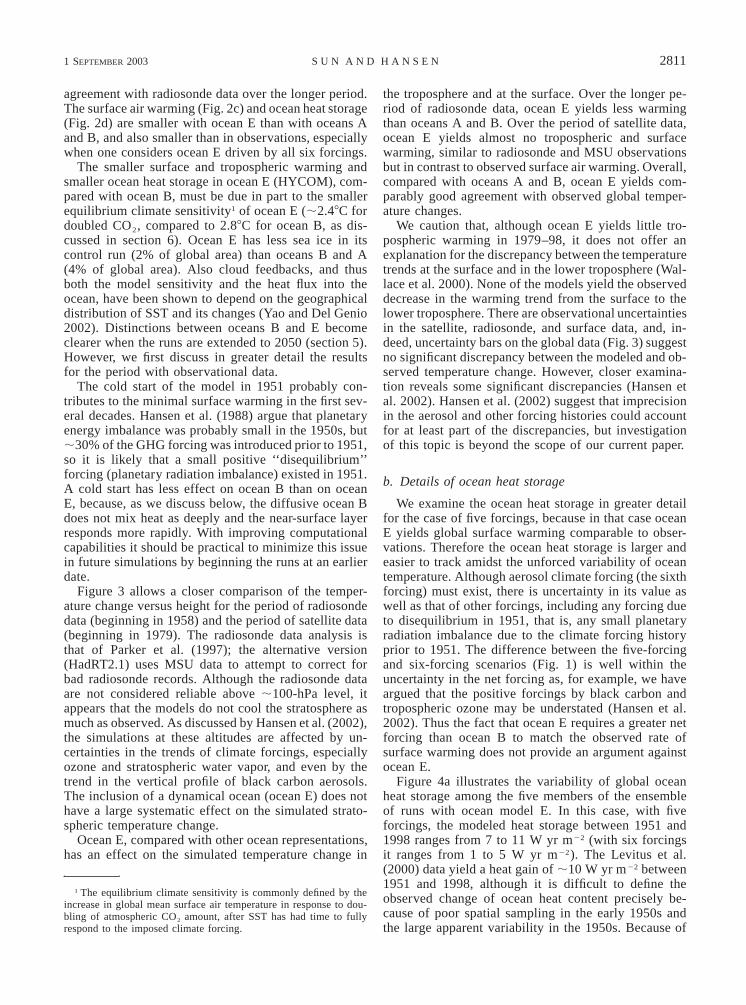
Figure 3 allows a closer comparison of the temper-ature change versus height for the period of radiosondedata (beginning in 1958) and the period of satellite data(beginning in 1979). The radiosonde data analysis isthat of Parker et al. (1997); the alternative version(HadRT2.1) uses MSU data to attempt to correct forbad radiosonde records. Although the radiosonde dataare not considered reliable above ;100-hPa level, itappears that the models do not cool the stratosphere asmuch as observed. As discussed by Hansen et al. (2002),the simulations at these altitudes are affected by un-certainties in the trends of climate forcings, especiallyozone and stratospheric water vapor, and even by thetrend in the vertical profile of black carbon aerosols.The inclusion of a dynamical ocean (ocean E) does nothave a large systematic effect on the simulated strato-spheric temperature change.

Ocean E, compared with other ocean representations,has an effect on the simulated temperature change in

1 The equilibrium climate sensitivity is commonly defined by theincrease in global mean surface air temperature in response to dou-bling of atmospheric CO2 amount, after SST has had time to fullyrespond to the imposed climate forcing.

the troposphere and at the surface. Over the longer pe-riod of radiosonde data, ocean E yields less warmingthan oceans A and B. Over the period of satellite data,ocean E yields almost no tropospheric and surfacewarming, similar to radiosonde and MSU observationsbut in contrast to observed surface air warming. Overall,compared with oceans A and B, ocean E yields com-parably good agreement with observed global temper-ature changes.

We caution that, although ocean E yields little tro-pospheric warming in 1979–98, it does not offer anexplanation for the discrepancy between the temperaturetrends at the surface and in the lower troposphere (Wal-lace et al. 2000). None of the models yield the observeddecrease in the warming trend from the surface to thelower troposphere. There are observational uncertaintiesin the satellite, radiosonde, and surface data, and, in-deed, uncertainty bars on the global data (Fig. 3) suggestno significant discrepancy between the modeled and ob-served temperature change. However, closer examina-tion reveals some significant discrepancies (Hansen etal. 2002). Hansen et al. (2002) suggest that imprecisionin the aerosol and other forcing histories could accountfor at least part of the discrepancies, but investigationof this topic is beyond the scope of our current paper.

b. Details of ocean heat storage

We examine the ocean heat storage in greater detailfor the case of five forcings, because in that case oceanE yields global surface warming comparable to obser-vations. Therefore the ocean heat storage is larger andeasier to track amidst the unforced variability of oceantemperature. Although aerosol climate forcing (the sixthforcing) must exist, there is uncertainty in its value aswell as that of other forcings, including any forcing dueto disequilibrium in 1951, that is, any small planetaryradiation imbalance due to the climate forcing historyprior to 1951. The difference between the five-forcingand six-forcing scenarios (Fig. 1) is well within theuncertainty in the net forcing as, for example, we haveargued that the positive forcings by black carbon andtropospheric ozone may be understated (Hansen et al.2002). Thus the fact that ocean E requires a greater netforcing than ocean B to match the observed rate ofsurface warming does not provide an argument againstocean E.

Figure 4a illustrates the variability of global oceanheat storage among the five members of the ensembleof runs with ocean model E. In this case, with fiveforcings, the modeled heat storage between 1951 and1998 ranges from 7 to 11 W yr m22 (with six forcingsit ranges from 1 to 5 W yr m22). The Levitus et al.(2000) data yield a heat gain of ;10 W yr m22 between1951 and 1998, although it is difficult to define theobserved change of ocean heat content precisely be-cause of poor spatial sampling in the early 1950s andthe large apparent variability in the 1950s. Because of


FIG. 3. Global mean annual mean temperature change for (top) 1958–98 and (bottom) 1979–98 based on linear trends. Model results arefor oceans A, B, and E with (a) five forcings and (b) six forcings. Radiosonde data become unreliable above ;100 hPa; alternative radiosondeanalyses HadRT2.0 and HadRT2.1 are from Parker et al. (1997). The surface observations (green triangles) are the land–ocean data of Hansenet al. (1999) with SST of Reynolds and Smith (1994) for ocean areas. The green bars for MSU satellite data (Christy et al. 2000) are twicethe standard statistical error adjusted for autocorrelation (Santer et al. 2000).


FIG. 4. (a) Global mean ocean heat content anomaly vs time relative to 1951 for Levitus et al. (2000) observations and for the ensembleof runs of ocean E with five climate forcings. (b) Global mean ocean temperature change vs depth between 1951 and 1998 from observationsand as simulated with five forcings for ocean B (ensemble mean) and ocean E (ensemble mean and individual runs).

the poor sampling in the early 1950s, Levitus et al.(2000) analyze the heat storage from 1955 onward. Con-sidering the variability in the simulated heat storagefrom run to run and the fact that the real world onlyran through this ‘‘experiment period’’ once, we concludethat the model yields reasonable agreement with ob-served heat storage, at least when the climate forcingin the model is sufficiently large to warm the surfacecomparable to observations.

We define heat storage as change of the total energycontent of the ocean. We evaluate the heat content fromthe interior ocean temperatures for oceans B and E andobservations. For ocean A we calculate the heat storagefrom the simulated energy fluxes at the ocean surface.Our unit for heat content, W yr m22, allows direct com-parison with the time integral of the climate forcings asdefined in Fig. 1.2 Thus, for example, for our estimatedaerosol forcing (Fig. 1), which grows approximatelylinearly from zero to 20.3 W m22 in 47 yr, the expectedchange in ocean heat storage is 27 W yr m22, consistentwith the change in heat storage mentioned in the par-agraph above.

None of the ensemble members yield decadal vari-ability of ocean heat storage as great as suggested bythe Levitus et al. (2000) data. Neither Barnett et al.

2 1 W yr ø 3.15 3 107 J; so 1 W yr m22 over the entire surfaceof the earth corresponds to 1.61 3 1022 J.

(2001) nor Levitus et al. (2001) obtained decadal var-iations in ocean heat storage similar to observations intheir climate model simulations, although Barnett et al.(2001) note that they found some decadal variationscomparable in magnitude to those observed. It is pos-sible that greater variability would have been obtainedin our runs if the ensemble members had not all beeninitiated within a 100-yr period of the model controlrun. Another possibility is that the decadal variabilityin the Levitus et al. (2000) data is an artifact of mea-surement error and incomplete sampling. Indeed, theresults in Fig. 2d for ocean A, in which ocean heatstorage is calculated from the modeled surface fluxesfor observed ocean temperatures, do not seem to beconsistent with the large swings in the observed oceanheat storage, as discussed in sections 6a(2) and 7b.

Figure 4b shows the depth profile of ocean heat stor-age for the same ensemble of runs as in Fig. 4a. Thereis substantial variability in the profile of heat storagewith ocean E, unlike the diffusive ocean B in which theocean warming declines monotonically with depth. In-deed, ocean E yields a minimum in ocean warming at;100 m depth, while the observed profile has a mini-mum at 150-m depth. One of the ensemble membershas cooling at 100 m. The individual model runs exhibitgreater variability with depth than the observationalanalysis. This might be in part a result of implicitsmoothing of the observations as a result of interpola-


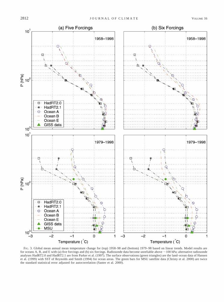
FIG. 5. Zonal ocean heat storage (W yr m22 averaged over theearth’s surface) between 1951 and 1998 for (top) the full ocean andsuccessive ocean layers. Observations are from Levitus et al. (2000).Climate models with oceans B and E are forced with five forcings.

tions and climatological values employed in data sparseregions (S. Levitus 2002, personal communication). Itis partly due to the fact that, because of the model drift,we obtained the heat storage by subtracting the controlrun, year by year, from the experiment run, thus in-creasing noise by approximately the square root of 2.

Figure 5 shows the latitude variation of ocean heatstorage for the full ocean (top two panels) and for suc-cessive layers. Ocean B yields close agreement with theobserved full-ocean global mean heat storage over thehalf-century (10 W yr m22), although the latitude var-iations are smoother than observations. Ocean E yieldsvariability of heat storage with latitude comparable tothat in observations, although the primary observed fea-ture, the maximum at 08–308N, is not captured in itsmagnitude. Ocean B has no heat storage at depths great-er than 1 km, as the ocean bottom was placed at thatlevel. We comment on the zonal mean heat storage inocean A after presenting the geographical distributionof heat storage in that model.

Figure 6 provides global maps of ocean heat storagebetween 1951 and 1998, as inferred by Levitus et al.(2000) from ocean temperature observations and as sim-ulated with different representations of the ocean. Thecalculated heat storage for oceans A and B of coursedoes not include any change in local heat storage dueto changes in horizontal ocean heat transport, althoughwith ocean A changes in ocean heat transport that arereflected in the SST may affect the vertical heat ex-change at the ocean surface and thus the calculated heatstorage. These limitations of oceans A and B are partof the reason that comparison of the sequence of oceanrepresentations is of interest.

The Levitus observational data reveal that the largeheat storage at latitudes 08–308N (Fig. 5) occurred es-pecially in the Atlantic and eastern Pacific Oceans (Fig.6). The negative change of heat content in the NorthAtlantic Ocean, with strong positive values at lowerlatitudes, suggests some slowing of the meridional cir-culation over the 47-yr period, but there are not obser-vations of the circulation adequate to verify that infer-ence. There are also regions of large heat storage in acircum-Antarctic belt, although observational data thereare limited and thus ocean temperature trends are moreuncertain.

The heat storage in ocean A (observed SST) climatesimulations has net positive storage in the Atlantic andPacific Oceans comparable to observations, but the geo-graphical pattern of heat storage in ocean A differsmarkedly from observations in the Pacific Ocean. Thisis not surprising as actual regions of heat storage dependin part upon convergence of ocean heat anomalies as-sociated with dynamical fluctuations in ocean transports.For example, waters off the west coast of the UnitedStates and Mexico warmed during the past two decades,probably because of increased net ocean heat transportinto that region. Associated warm SST anomalies causethe sensible and latent heat fluxes into the atmosphere

from that ocean region to increase in the ocean A climatesimulations, thus yielding a negative ocean heat contentchange in that model. Similarly, the Baffin Bay–Green-land Sea region draws extra heat from the atmospherein ocean A climate simulations because the SST has


FIG. 6. Global distribution of ocean heat storage during the interval 1951–98. Observations are from Levitus et al. (2000). Climatemodels with oceans A, B, and E are forced with five forcings.

cooled there in recent decades. In reality, that oceanregion may have transmitted extra heat to the atmo-sphere that helped warm Eurasia in recent decades, butproper modeling of this phenomenon requires simulat-ing anomalies of ocean heat transports and it probablyalso requires realistic simulation of dynamical interac-tions with the stratosphere. Note in Fig. 5 that, despitethese regions where the sign of the surface heat fluxanomaly differs from the change in ocean heat content,ocean A qualitatively captures much of the latitudinalvariation of ocean heat storage, which suggests thatmuch of the ocean transport of heat anomalies is zonal.The spikes in heat storage calculated with ocean A inregions of sea ice are a result of changing sea ice areain the dataset of Rayner et al. (2003). The sea ice trendsare very uncertain, but the absence of correspondingheat storage spikes in the Levitus et al. data does notrule against the reality of the sea ice changes. A largechange in ocean heat storage, as calculated with oceanA, should occur in regions where sea ice cover changes,but within the real ocean the heat content anomaly islikely to be smoothed by ocean transports.

Ocean B yields a distribution of heat storage that ismuch more featureless than observations, which is notsurprising, given the model’s lack of dynamical oceanvariability. Atmospheric dynamics by itself could pro-duce geographic features in the ocean heat storage, and,for example, one might hope that the Q-flux modelwould produce the observed negative heat storage in

the Baffin Bay region, if the observed trend in the ArcticOscillation is driven by increasing greenhouse gases(Shindell et al. 2001b). However, the rigid top of theSI2000 model at 10 hPa prevents realistic simulation ofthat phenomenon in the present simulations with any ofoceans A, B, and E.

Oceans B and E both produce a maximum in heatstorage in a circum-Antarctic belt, as in observations,with the ocean E results appearing more realistic (Fig.6). Note the large variability in the heat storage fromrun to run. Runs 4 and 5 of ocean E have a number ofgeographic features in common with the observations,including the positive heat content anomalies in the east-ern Pacific Ocean. The warm waters off the U.S. WestCoast have had biological consequences that have beensuggested to be a consequence of global warming(Roemmich and McGowan 1995). The variabilityamong the ensemble members in our simulations for1951–2000, by itself, would suggest that this warmingis a dynamical fluctuation, rather than a forced change,and thus it is as likely as not to revert to cooler tem-peratures in coming years. However, the simulationsbelow for the next 50 yr present a rather different con-clusion.

5. Extended simulations

We extend ensembles of the coupled atmosphere–ocean simulations to 2050 using both the strong (BAU)


and weak (ALT) forcing scenarios. For the sake of in-terpreting the results we also compare a doubled CO2

simulation using the HYCOM ocean to a doubled CO2

run using the Q-flux ocean.

a. Simulations to 2050

Figure 7 shows the ensemble mean transient responseof the coupled atmosphere–ocean model with ocean E.During 1951–2000 the climate forcings are the five-forcing and six-forcing scenarios (section 3), so the leftside of the figure summarizes results presented in section4. Two five-member ensembles of runs were extendedto 2050 using the BAU and ALT climate forcing sce-narios, which, respectively, add forcings of 2.9 and 1.1W m22 in the 50 yr (section 3). Ocean initial conditionsin 2000 were those from the 1951–2000 five-forcingruns. The transient responses to these forcing scenariosare shown in the right half of Fig. 7.

The stratosphere cools almost 18C in the BAU sce-nario but only a few tenths of a degree in the ALTscenario, in accord with their increases of CO2. If theeffect of anticipated partial ozone recovery (from chlo-rine-induced O3 depletion during the past 25 yr) wereincluded, the stratospheric temperature would be essen-tially flat during the next 50 yr in the ALT scenario.These results for stratospheric temperature are similarto those obtained with ocean B by Hansen et al. (2002).

The troposphere and surface warm by only 0.38–0.48Cin the next 50 yr in the ALT scenario, but by more than18C in the BAU scenario. These warmings are less thanthose obtained with ocean B using the same forcingscenarios (Hansen et al. 2002). For example, the warm-ing obtained by Hansen et al. (2002) for the ALT sce-nario with ocean B is 3/48C, about twice as large as thewarming with ocean E. Consistent with the smaller sur-face warming with ocean E, the planetary energy im-balance by 2050 increases to ;1.3 W m22 and almost2 W m22 in the ALT and BAU scenarios, respectively,which compares with 0.8 and 1.4 W m22 for the samescenarios with ocean B (Hansen et al. 2002).

1) HEAT STORAGE

Figures 8 and 9 contrast the ocean heat storage ofoceans B and E during the period 2000–50. Both modelssequester heat most effectively in high-latitude regions.The prime difference between the two oceans is thatocean E stores more heat at low latitudes, especially inthe eastern Pacific Ocean, but also in the western Pacificand Indian Oceans. The greater low-latitude heat storagein ocean E occurs in the upper 500 m (Fig. 9). Table 1summarizes the observed and modeled global ocean heatstorage.

Oceans B and E have similar latitudinal distributionsof depth-integrated heat storage (Fig. 9). However, inocean B a greater amount of heat builds up in the 500–1000-m layer. If an artificial bottom had not been placed

at 1 km in ocean B, heat would have penetrated intothe lower ocean layers, providing better correspondencewith ocean E. This would have 1) increased the mixingof heat from the top ocean layers into the deeper ocean;2) increased the total ocean heat storage, that is, the heatflux into the ocean surface; and 3) decreased the globalsurface warming.

The large observed ocean heat storage at low latitudes(Figs. 5 and 6) tends to support the larger magnitude ofstorage at low latitudes in ocean E, as opposed to oceanB. Larger mixing coefficients may be appropriate at lowlatitudes, where most of the mixing occurs via quasi-horizontal transports (Ledwell et al. 1998). However,Forest et al. (2002) show that there is a large range ofocean heat uptakes among the different ocean modelsand, given the uncertainties in observed heat uptake, itseems best to leave Q-flux coefficients as they are. In-deed, Fig. 5 suggests that the Q-flux model does a goodjob for heat uptake, so the only change needed may beto place the ocean bottom at 4 km.

There are some consistent features in the geographicalpatterns of simulated heat storage with ocean E thatimply predictions for climate change in the coming half-century. Four of the five ensemble members for the ALTscenario and all five of the BAU ensemble membershave increased heat storage along the west coast of theAmericas. Similarly, both of the forcing scenarios con-sistently yield a region of decreased heat storage in thePacific Ocean between about 308 and 608N. Theseanomaly patterns have been observed during recent de-cades and are often suggested to be cyclical. However,our climate simulations suggest that a tendency to havethese patterns may be a consequence of the forcings,and thus these ocean temperatures may be a harbingerof climate patterns that will tend to exist in comingdecades, rather than being dynamical fluctuations. Caiand Whetton (2001) noted a shift in observed warmingfrom higher latitudes to the El Nino regions, and theypresented modeling evidence that the shift was drivenby greenhouse gases and was likely to continue.

The large heat storage in both ocean models B andE in the first half of the twenty-first century, despite thevery modest increase in climate forcings in the ALTscenario, is a reflection of the current planetary radiationimbalance of 3/4 W m22, which was inferred severalyears ago (Hansen et al. 1997) and which is containedin the climate simulations for both ocean models (Fig.7d). If ocean heat storage is monitored accurately incoming decades it will provide an invaluable diagnosticof the climate system, both for the purpose of refiningour knowledge of the planetary energy imbalance,which is important for determining future global climatechange, and for the purpose of checking the ocean mod-els’ abilities to simulate the distribution of heat anom-alies, which is necessary for predicting the geographicaldistribution of climate change.


2) OCEAN TRANSPORTS

Figure 10 shows the northward heat transport in theocean basins3 and globally for ocean E simulations. Re-sults are shown for the past decade with the five-forcingsscenario and for 2045–55 with the strongest (BAU) forc-ing scenario. The simulated heat transports are mostlyin agreement with analyses of MacDonald (1998) andTrenberth and Caron (2001), within the margin of ob-servational error. We do not find a noticeable sensitivityof the ocean transport to the climate forcings over therange of forcings that we considered.

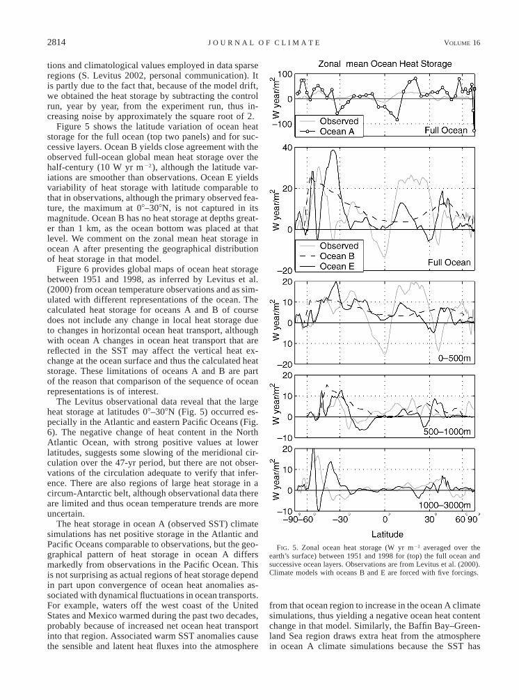
We also find no significant impact of the forcings onthe ocean E simulated overturning rate and meridionalheat flux in the Atlantic Ocean, as shown in Fig. 11.This is consistent with the results of Sun and Bleck(2001), who found that ocean E maintains a stable ther-mohaline circulation (THC) in a 2 3 CO2 experimentthat started from observed ocean conditions, but it dif-fers from a number of models that project the ther-mohaline circulation to weaken in the twenty-first cen-tury. Wood et al. (1999) and Dixon et al. (1999) foundthe thermohaline circulation to slow after 150–200 yr;it also slowed but then recovered by year 500 in theexperiment of Manabe and Stouffer (1994). On the otherhand, Latif et al. (2000) and Gent (2001) did not finda slowdown of the thermohaline circulation. The widerange of responses of the thermohaline circulationamong different climate models is illustrated in Fig. 9.21of Houghton et al. (2001).

The strength of oceanic overturning is controlled bymany factors including the intensity of thermal and ha-line forcing. Some model studies have shown that in-creasing surface freshwater fluxes into the North At-lantic are the primary reason for the slowdown of theAtlantic THC in simulations of global warming (Wiebeand Weaver 1999; Dixon et al. 1999), while in othersimulations it appears to be the surface warming trendthat causes the THC to weaken (Mikolajewicz and Voss2000). We see in the BAU scenario an increase in bothprecipitation and evaporation in the North Atlantic inocean E, which leads to a small overall change in fresh-water fluxes. In our experiments, the thermohaline sig-nals, rather than being trapped near the surface, fairlyquickly propagate down the water column in the north-ern North Atlantic. As a result, the vertical stratificationin that region remains similar to that in the control runand thus does not impede the sinking motion, which isan essential part of the Atlantic THC. The positive feed-back aspects of this process are rather obvious: a strongTHC is able to maintain the weak stratification in thesinking region and hence can maintain itself, while aTHC that is anemic to begin with may come to a halt

3 To remove the ambiguity associated with the nonzero meridionalmass flux in both the Pacific and Indian Oceans south of the Indo-nesian passage, the heat flux curves for both basins have been adjustedby the amount of heat transported through that passage.

during global warming. We note that the Atlantic ther-mohaline circulation in our simulation (;22 Sv) isstrong compared with some recent observational anal-yses (Ganachaud and Wunsch 2000), but there is a largeuncertainty in the observed value.

The range of results among different ocean modelsis not surprising, as vertical mixing is known to play amajor role in long-term, planetary-scale ocean dynamics(Stommel and Arons 1960), and circulation systemsdriven by buoyancy forces are particularly sensitive tothe rate at which buoyancy anomalies are diffused inthe ocean. In this vein, Houghton et al. (2001) suggestthat differences in subgrid-scale mixing parameteriza-tion account for much of the difference in the rate ofsurface warming. Some vertical mixing is likely to occuras a result of vertical advection whose numerical im-plementation varies widely among ocean models. Iso-pycnic coordinate ocean models, due to the quasi-La-grangian nature of their coordinate surfaces, have aninherent advantage in suppressing the numerical dia-pycnal mixing associated in the traditional fixed-gridmodels with the passage of internal waves (Bleck 1998).Gent et al. (2002) also found improvement in modeledmeridional overturning circulation with a new param-eterization of isopycnal mixing in a z-coordinate model,and the strength of the simulated thermohaline circu-lation with such a parameterization did not slow downin the global warming scenario (Gent 2001).

b. Doubled CO2 experiment

Interpretation of the transient climate experiments isaided by comparison of equilibrium simulations withoceans B and E using a strong identical forcing. In ourdoubled CO2 experiment we add 1% CO2 yr21 until 23 CO2 is reached at year 70, when the forcing is 3.9W m22, after which time the CO2 concentration is keptfixed.

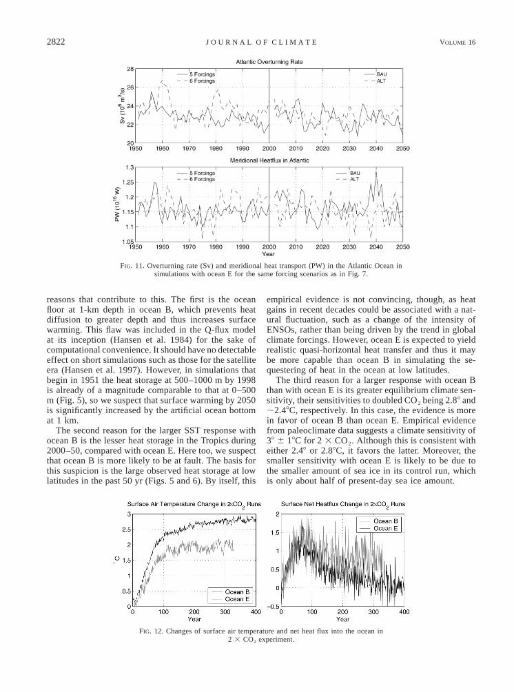
Ocean B reaches equilibrium global surface temper-ature response (2.88C) by year 400, when the heat fluxinto the ocean has approached, but not quite reached,zero (Fig. 12). Ocean E, after 300 yr, has a remainingenergy imbalance of ;0.7 W m22. Thus the warmingof 28C at year 300 is the response to ;3.2 W m22

forcing, which implies that the equilibrium sensitivityis ;2.48C for 2 3 CO2. That sensitivity is consistentwith the 2.88C sensitivity of the Q-flux model, becauseof the different amounts of sea ice in the control runs.The ocean E control run has sea ice covering 2% of theworld area, while the sea ice covers 4% of the globe inthe ocean B control run. We can judge the impact ofthe sea ice cover from an alternative version of oceanB used by Hansen et al. (2002). This alternative versionhad 6% sea ice in the control run, but otherwise identicalphysics with the Q-flux run used here. The change ofsea ice from 4% to 6% of the global area increased thesensitivity from 2.88 to 3.28C for 2 3 CO2.

Other things being equal, a model with 2.48C sen-


FIG. 7. Ensemble mean transient response of the coupled model with ocean E. During 1951–2000 the climate forcings are the five forcingsand six forcings (tropospheric aerosols added) defined in Fig. 1. The extensions to 2050 employ the BAU (2.9 W m 22) and ALT (1.1 Wm22) forcings.

sitivity should approach equilibrium much faster than amodel with 2.88C sensitivity, as the response time isproportional to the square of the equilibrium sensitivity(Hansen et al. 1985). Furthermore, at any given timethe heat flux into the ocean is larger in a higher-sen-

sitivity model, other things being equal. Figure 12bshows that other things are not equal in oceans B andE. The flux into the ocean surface in ocean E keeps upwith that for ocean B for the first several decades, andafter 50 yr it exceeds that for model B. From the results


FIG. 8. Ocean heat storage (W yr m22) during 2000–50 in oceans B and E for the ALT climate forcing scenario.

in section 5.1, we know there are two reasons for this:1) the shallowness of ocean B model (1 km), and 2) thedifferent vertical diffusions in two oceans, especiallythe more rapid heat uptake at low latitudes in ocean E.Figure 12b shows that these effects are sufficient to

make the heat storage of the model with lower sensi-tivity (i.e., ocean E) slightly exceed that of ocean B onthe 100-yr timescale. This result is consistent with thegreater heat storage in ocean E in the transient climateexperiment during the period 2000–50 (Table 1).


FIG. 9. Zonal ocean heat storage (W yr m22 averaged over theearth’s surface) during 2000–50 in oceans B and E for the ALT climateforcing scenario.

6. Discussion

We aim to learn something about the effect of theocean representation on ocean heat uptake and climateresponse time by contrasting results from experimentsthat use a variety of oceans driven by the same atmo-sphere and climate forcings. Conclusions from the pre-sent simulations, for oceans A, B, and E, are constrainedby the brevity of the simulations and limitation to a

single dynamical ocean model. Some of the computa-tions are necessarily different for these three ocean rep-resentations, so we clarify that here.

a. Ocean A

1) GLOBAL OCEAN HEAT STORAGE

The climate model with ocean A is nearly in radiationbalance at the beginning of the simulation, that is, in1951. This near balance occurs because the parameterin the model that controls cloud cover (Uoo, the min-imum grid-box mean humidity at which clouds beginto form) was chosen with the objective of radiation bal-ance. However, even a small planetary radiation im-balance needs to be evaluated, because it affects theocean heat storage. We can determine the radiation im-balance in the climate model by making a long run withfixed 1951 SST and atmospheric composition. However,it is better to use the mean SST for several years centeredon 1951 to minimize the effect of interannual SST var-iability, such as El Nino.

Specifically, Hansen et al. (2002) made a 20-yr sim-ulation with 1951 atmospheric composition and withSST and sea ice based on the 10-yr mean of Rayner etal. (2003) centered on 1 January 1951, obtaining a fluximbalance of 20.175 W m22. In other words, in thecontrol run the planet continually gives out heat to spaceat an annually averaged rate of 0.175 W m22, as thefixed ocean temperature does not respond to the energyloss. The standard deviation of the annual mean globalradiation balance was 0.18 W m22, so, for the assumedSST distribution, the uncertainty in the calculated fluximbalance is of order 0.04 W m22. Thus, if we wish toassume that the planet was in energy balance in the 1951era and use the energy imbalance in the transient 1951–98 ocean A simulations to calculate ocean heat storage,we must add 0.175 W m22 to the calculated fluxes.

The resulting ocean heat storage in ocean A is shownby the green curve in Fig. 13, for the case of the sixclimate forcings of Fig. 1. The heat storage between1951 and 1998 is ;3 W yr m22, which is much lessthan the observed heat storage of ;10 W yr m22. Wecould achieve greater heat storage by increasing thegrowth of the net climate forcing over the period 1951–98. For example, if there were an unknown climate forc-ing that increased linearly by 0.2 W m22 over the 47-yr period it would add to the heat storage 4.7 W m22.Thus a forcing that increased by 0.3–0.4 W m22 overthe 47-yr period would be sufficient to yield agreementwith the observed ocean heat storage. Such an error inour net climate forcing cannot be ruled out.

However, we believe that a more likely interpretationis that the planet was not in energy balance in 1951.The red curve in Fig. 13 shows that an energy imbalanceof ;0.18 W m22 (energy coming into the planet) isneeded for approximate agreement with observed oceanheat storage. Because of the uncertainty in the climate


TABLE 1. Ocean heat storage (W yr m22) in observations (Levitus et al. 2000) and in ocean models B and E. The models are driven byfive forcings during 1951–98 and by the ALT forcing scenario during 2000–50.

Ocean depth

1951–98

Observed Ocean B Ocean E

2000-50

Ocean B Ocean E

0–500 m500–1000 m

1000–1500 m1500–2000 m2000–2500 m2500–3000 m

Full ocean

5.02.30.70.40.20.08.6

6.04.0————

10.0

5.61.20.70.60.40.38.1

13.214.4————

27.6

17.08.23.91.81.40.6

30.8

FIG. 10. Northward heat transport in three ocean basins and globally in ocean E simulationsfor the past decade and simulations for the middle of the twenty-first century with a strong (BAU)forcing scenario.

forcing, this inferred energy imbalance is uncertain byan amount comparable to the estimated imbalance. Allwe can say is that, for our best estimate of climateforcing, we require a planetary energy imbalance of10.18 W m22 in 1951 to obtain the ocean heat storagemeasured by Levitus et al. (2001). An energy imbalanceof 0.18 W m22 in 1951 can be compared with the im-balance of 0.65 W m22 in 1979 inferred by Hansen etal. (1997) and the imbalance of 3/4 W m22 in 1998inferred by Hansen et al. (2002) and by our presentsimulations. These values are consistent, as only ;30%of the present greenhouse gas climate forcing was in-troduced prior to 1951 and the earlier forcing was addedover a longer period.

2) TEMPORAL AND GEOGRAPHICAL VARIATIONS

The calculated global heat storage with ocean A asa function of time (Fig. 2d) does not yield the strongdecadal fluctuations in the Levitus et al. (2000) data,such as the rapid decrease in the mid-1950s, increasein the early 1970s, and decrease in the early 1980s.Although fluctuations in ocean dynamics can cause fluc-tuations in ocean heat content unrelated to climate forc-ings, the ocean heat content fluctuations must be ac-companied by a flux anomaly across the ocean surface.However, when we use observed SST to calculate thefluxes, we do not find anomalies corresponding to thesesupposed rapid ocean heat content changes. Therefore,

we suggest that the ocean A calculations cast doubt onthe reality of these decadal fluctuations in ocean heatcontent. Alternatively, our climate model may not pro-duce correct flux anomalies as a function of SST. Forexample, there may have been real-world flux anomaliesassociated with wind anomalies or cloud cover anom-alies that are not captured by our model. A third pos-sibility is error in the specified sea ice history, becausesea ice changes strongly influence ocean–atmosphereheat exchange. Analysis of the regional distribution ofthe heat content fluctuations may discriminate amongalternative interpretations.

The local heat storage anomalies calculated withocean A account only for the simulated exchange ofheat at the ocean surface. Thus comparison of the oceanA result with observed ocean heat content yields infer-ences about ocean dynamical heat transports. For ex-ample, the surface heat fluxes in ocean A (Fig. 6) havethe eastern Pacific Ocean (a region with good obser-vations) disgorging heat at a substantial rate in just theregion where the Levitus et al. (2000) analyses showthat the ocean heat content also increased markedly. Thisimplies that there was a substantial horizontal transportof heat by the ocean into this region.

b. Ocean B

The SST response to climate forcings is larger forocean B than for ocean E. We have identified three


FIG. 11. Overturning rate (Sv) and meridional heat transport (PW) in the Atlantic Ocean insimulations with ocean E for the same forcing scenarios as in Fig. 7.

FIG. 12. Changes of surface air temperature and net heat flux into the ocean in2 3 CO2 experiment.

reasons that contribute to this. The first is the oceanfloor at 1-km depth in ocean B, which prevents heatdiffusion to greater depth and thus increases surfacewarming. This flaw was included in the Q-flux modelat its inception (Hansen et al. 1984) for the sake ofcomputational convenience. It should have no detectableeffect on short simulations such as those for the satelliteera (Hansen et al. 1997). However, in simulations thatbegin in 1951 the heat storage at 500–1000 m by 1998is already of a magnitude comparable to that at 0–500m (Fig. 5), so we suspect that surface warming by 2050is significantly increased by the artificial ocean bottomat 1 km.

The second reason for the larger SST response withocean B is the lesser heat storage in the Tropics during2000–50, compared with ocean E. Here too, we suspectthat ocean B is more likely to be at fault. The basis forthis suspicion is the large observed heat storage at lowlatitudes in the past 50 yr (Figs. 5 and 6). By itself, this

empirical evidence is not convincing, though, as heatgains in recent decades could be associated with a nat-ural fluctuation, such as a change of the intensity ofENSOs, rather than being driven by the trend in globalclimate forcings. However, ocean E is expected to yieldrealistic quasi-horizontal heat transfer and thus it maybe more capable than ocean B in simulating the se-questering of heat in the ocean at low latitudes.

The third reason for a larger response with ocean Bthan with ocean E is its greater equilibrium climate sen-sitivity, their sensitivities to doubled CO2 being 2.88 and;2.48C, respectively. In this case, the evidence is morein favor of ocean B than ocean E. Empirical evidencefrom paleoclimate data suggests a climate sensitivity of38 6 18C for 2 3 CO2. Although this is consistent witheither 2.48 or 2.88C, it favors the latter. Moreover, thesmaller sensitivity with ocean E is likely to be due tothe smaller amount of sea ice in its control run, whichis only about half of present-day sea ice amount.


FIG. 13. Ocean heat content anomaly (W yr m22) averaged over the surface of the earth. Zeropoint for model is 1951. Zero point for observations is 1950–59 mean.

Larger uptake of heat in ocean E than in ocean B isnot surprising. Diffusion in ocean B, based on empiricalfit to transient tracer data and meant to represent theeffect of all mixing processes, varies from about 0.1cm2 s21 at low latitudes to 15 cm2 s21 in the NorthAtlantic Ocean and in the Southern Ocean (Hansen etal. 1984). Prescribed diapycnal diffusion in ocean E(0.003 cm2 s22 3 N21) is generally smaller than thetotal diffusion in ocean B, but the net effect of all mixingprocesses in ocean E yields a greater effective diffusion,at the high end of the range of ocean models examinedby Sokolov et al. (2003), as discussed below. Analysisof the ocean heat uptake processes is beyond the scopeof the present paper, but we anticipate that new longersimulations that correct several flaws in the present runs,include other dynamical ocean models, and test alter-native turbulent mixing schemes, will provide fodderfor useful analyses.

Overall, comparison of the ocean B heat storage withobservations and with ocean E provides a positive as-sessment of ocean B capabilities. The too-shallow bot-tom is trivial to correct and the tropical mixing ratescould be modified if more well-founded values weredefined. The Q-flux model perhaps has been unjustlydenigrated in the past, for example, not being consideredas a coupled atmosphere–ocean model and excludedfrom Houghton et al. (1996) comparisons, despite otherlimitations of many dynamical oceans, such as flux cor-rections and the absence of polar coverage. However,we consider ocean B’s principal value not as a com-petitor to dynamic ocean models, but rather as a com-panion that helps to improve our understanding of themechanisms and significance of results from more re-alistic ocean models.

c. Ocean E

The heat sequestration in ocean E has a good deal incommon with observed heat storage in the past halfcentury. The profiles of heat storage versus depth (Fig.4) and versus latitude (Fig. 5) are generally consistentwith the observational analysis of Levitus et al. (2000).Geographic patterns of simulated heat storage (Fig. 6)are not quite as faithful to observations. The positiveheat storage in the circum-Antarctic belt and heat lossin the North Pacific Ocean are captured by all runs ofthe model, and some of the individual runs capture thepositive heat storage off the west coast of North Americaand in the North Atlantic Ocean. Overall, the simulatedheat storage is sufficiently realistic that it perhaps addsto the credibility of the model already documented bySun and Bleck (2001), and it suggests that it would beinteresting to carry out global and regional climate stud-ies using this ocean model combined with an atmo-spheric model capable of representing the primary cli-mate forcings including those operating via the strato-sphere.

d. Reconciliation of oceans A, B, and E

Ocean A provides evidence that the earth was out ofradiation balance in 1951 by, we estimate, ;0.2 W m22.In lieu of starting climate simulations at an earlier date,climate models initiated in 1951 could include a positiveradiative input of that magnitude. This is not a perfectsolution to the cold start problem, as it does not providea temperature anomaly profile within the ocean, but itshould be a useful approximation.

If our ocean E simulations had included this ‘‘initialimbalance’’ forcing, global warming by 2000 probably


would have increased ;0.18C (more than half of theequilibrium response should be achieved in 50 yr) bring-ing the result into closer agreement with observations(Fig. 2). Increased climate sensitivity of the model (ifit had 4% sea ice instead of 2%) should add a fewhundredths of a degree to the response over 50 yr. Givenuncertainties in the climate forcings and observed tem-perature change, as well as unforced variability of cli-mate, the correspondence with observed global tem-perature change is excellent.

If the same initial planetary energy imbalance hadbeen included in the ocean B simulations of Hansen etal. (2002), it would have increased global warming0.18C, making the simulated warming somewhat largerthan observed. However, the other factors discussedabove, the need to extend the ocean depth to 4 km andperhaps increase the mixing rate in the Tropics, wouldreduce the surface warming. The net change from allthese refinements is probably small.

7. Implications

a. Projected climate change

Based on results from the different ocean models, weestimate that the global warming in the next 50 yr withthe alternative scenario of climate forcings (1.1 W m22

added forcing between 2000 and 2050) will be only;0.58 6 0.28C. The partly subjective error estimateassumes that the forcing is precise and thus the errorincorporates uncertainties in the atmosphere and oceanrepresentations including climate sensitivity. The warm-ing is less than the 0.758 6 0.258C obtained with oceanB (Hansen et al. 2002), because the version of ocean Bused in that study is at least somewhat deficient in itsability to sequester heat. The warming is greater thanthe 0.38–0.48C in our current ocean E simulation be-cause of the deficient sea ice in ocean E (and thus lowclimate sensitivity) and the remaining effect in 2000–50 of the 1951 cold start of that model.

We stress that we are not predicting attainment of thealternative scenario of climate forcings, although wethink such a scenario is achievable. It is an ambitiousscenario for slowing the growth rate of climate forcingsthat would require non-CO2 forcings to be no greaterin 2050 than they are today (Hansen et al. 2002). Thegrowth rate of atmospheric CO2 in this scenario is onlyslightly larger in the next two decades than it was inthe 1990s and it then begins to decline slowly. The netforcing is less than in any Houghton et al. (2001) sce-nario.

Increased sequestering of heat by the ocean not onlyreduces surface warming in coming decades, it also in-creases the predicted planetary disequilibrium, that is,the earth’s energy imbalance. Even with the moderateclimate forcing of the alternative scenario and a lowclimate sensitivity of 2.48C for 2 3 CO2, the net fluxof energy into the planet increases to ;1.3 W m22 in

2050, considerably larger than the 0.75 W m22 estimatedfor the earth’s current imbalance. The fact that more ofthe greenhouse heating is sequestered and less appearsas near-term warming is a consequence of the deep mix-ing and long response time of the presumably morerealistic ocean representation of ocean E. This longerocean response time has both good and bad sides froma practical perspective. It provides an opportunity toquantitatively verify the track that the earth’s climate ison, provided appropriate observations are obtained, anda longer period to act before the largest consequencesof global warming will occur. The bad side of the slowerresponse is an increase in the amount of warming thatis ‘‘in the pipeline’’ but not yet realized. However, thisslower response also means that, if the emissions of CO2

are reduced, the ocean has a longer time to take up CO2

and thus avoid the largest climate change.The importance of oceanic sequestering of heat and

the implications for climate response time raise the ques-tion of how reliable the ocean E result is. Sokolov etal. (2003) compare 11 atmosphere–ocean GCMs andfind that their measure of oceanic heat uptake, ,1/2K n

where is an effective global diffusion coefficient,1/2K n

varies from 2 to 5 cm s21/2 among models, with oceanE at the large end of this range. Empirical data analyzedby Forest et al. (2002) tend to favor the higher Kn values,but all of the models are within the range of observa-tional uncertainty. The Levitus et al. (2000) data forheat uptake seem consistent with our ocean E simula-tion, but do not verify the rate of heat uptake. Althoughwe believe that the ocean E results are realistic, the rateof ocean uptake is uncertain and deserves high priorityin modeling and observational analyses.

b. Needed observations

This study highlights the importance of full-oceanheat storage measurements. The current rate of changeof ocean heat content provides a measure of the ‘‘re-sidual’’ global climate forcing, that is, the existing in-tegrated (net) forcing of the global climate system. Wedefine the residual forcing as that portion of long-termclimate forcings that has not yet been responded to. Theresidual forcing is equal to the current planetary energyimbalance excluding transitory effects such as El Ninosand volcanos. Multiplied by global climate sensitivity,estimated to be 3/48 6 1/48C (W m22)21, the residualforcing yields the additional global warming that is inthe pipeline, that is, the warming that will occur withoutany further change of atmospheric composition.

The increased heat content of ;7 W yr m22 in the1990s in the Levitus et al. (2000) data is nominallyconsistent with our estimated current planetary energyimbalance of 0.75 W m22, but it is somewhat largerthan the heat storage in our simulations, which is re-duced by the effect of the Pinatubo eruption. The oceanheat gain over the past half-century is in good agreementwith the mean planetary energy imbalance in our climate


model simulations. However, there are decadal varia-tions in the Levitus et al. (2000) data that are not as-sociated with known climate forcings and are not re-produced with any of the ocean models. It is desirableto have more complete ocean measurements, with bettergeographic and depth sampling, because the existingnetwork could misinterpret a dynamical redistributionof heat as a change of ocean heat content.

The full-ocean depth needs to be monitored. The in-ternational Argo project (Roemmich and Owens 2000)will deploy about 3000 profiling floats that will measuretemperature to a depth of 1500–2000 m every 10 dayson a near-global basis. Although this will be helpful, itmust be supplemented by deep-ocean measurements.Because the deeper ocean changes more slowly, the fre-quency of surveying the deep ocean does not need tobe as great as for the upper ocean.

Climate forcing agents must be monitored so that wecan understand the causes of changes in ocean heat con-tent. Knowledge of the principal individual forcingagents is also information that decision makers wouldrequire, should they wish to alter the course of climatechange. Most greenhouse gases, except troposphericozone, are well measured, but a large improvement inthe quality of measurements of aerosols and their effectson clouds is needed if we are to quantify their changingforcing. There are plans for measurements of aerosolsand cloud particles from operational satellites in about2010 with sufficient information on the microphysics toinfer composition specific information (Haas et al.2002), as well as plans for measuring troposphericozone. Thus if ocean heat content measurements areimproved, it may be possible to begin to quantify muchbetter the changing planetary radiation imbalance andits causes within about a decade.

c. Future simulations

This study provides an indication of the potential mer-it of climate simulations in which identical forcings areused to drive climate models with alternative treatmentsof key parts of the climate system. Although we con-sidered here only three alternative ocean representa-tions, our intention, as discussed by Hansen et al. (1997,2002), is to include other dynamic ocean models, morerealistic stratospheric representations, and models withlower and higher climate sensitivity (via altered cloudfeedbacks). This approach differs from comparison ofmodels of different laboratories, because the latter in-volve uncountable differences among the model phys-ical representations, which thus makes it difficult toidentify the causes of different simulated climate re-sponses. The simulations will be more useful if theybegin early enough to avoid the cold start problem andif the atmosphere realistically represents troposphere–stratosphere interactions.

Acknowledgments. We are indebted to Rainer Bleck,the architect of the HYCOM model, for his guidanceand suggestions; and Wil Burns, Peter Gleick, PeterStone, and two anonymous referees for reference ma-terial and suggestions for the manuscript. This researchwas supported by the NASA climate and oceanographyprograms managed by Tsengdar Lee and Eric Lind-strom.

REFERENCES

Arfken, G., 1970: Mathematical Methods for Physicists. 2d ed. Ac-ademic Press, 815 pp.

Barnett, T. P., D. W. Pierce, and R. Schnur, 2001: Detection of an-thropogenic climate change in the world’s oceans. Science, 292,270–274.

Bleck, R., 1998: Ocean modeling in isopycnic coordinates. OceanModeling and Parameterization, E. P. Chassignet and J. Verron,Eds., Kluwer Academic, 423–448.

——, 2002: An oceanic general circulation model framed in hybridisopycnic–Cartesian coordinates. Ocean Model., 4, 55–88.

——, and S. G. Benjamin, 1993: Regional weather prediction witha model combining terrain-following and isentropic coordinates.Part I: Model description. Mon. Wea. Rev., 121, 1770–1785.

——, C. Rooth, D. Hu, and L. Smith, 1992: Salinity-driven ther-mocline transients in a wind- and thermohaline-forced isopycniccoordinate model of the North Atlantic. J. Phys. Oceanogr., 22,1486–1505.

Boyle, J. S., 1998: Evaluation of the annual cycle of precipitationover the United States in GCMs: AMIP simulations. J. Climate,11, 1041–1055.

Cai, W., and P. H. Whetton, 2001: A time-varying greenhouse warm-ing pattern and the tropical–extratropical circulation linkage inthe Pacific Ocean. J. Climate, 14, 3337–3355.

Christy, J. R., R. W. Spencer, and W. D. Braswell, 2000: MSU tro-pospheric temperatures: Dataset construction and radiosondecomparisons. J. Atmos. Oceanic Technol., 17, 1153–1170.

Cubasch, U., K. Hasselmann, H. Hock, E. Maier-Reimer, U. Miko-lajewicz, B. D. Santer, and R. Sausen, 1992: Time-dependentgreenhouse warming computations with a coupled ocean–at-mosphere model. Climate Dyn., 8, 55–69.

Dixon, K. W., and J. R. Lanzante, 1999: Global mean surface airtemperature and North Atlantic overturning in a suite of coupledGCM climate change experiments. Geophys. Res. Lett., 26,1885–1888.

——, T. L. Delworth, M. J. Spelman, and R. J. Stouffer, 1999: Theinfluence of transient surface fluxes on North Atlantic overturn-ing in a coupled GCM climate change experiment. Geophys.Res. Lett., 26, 2749–2752.

Forest, C. E., P. H. Stone, A. P. Sokolov, M. R. Allen, and M. D.Webster, 2002: Quantifying uncertainties in climate system prop-erties with the use of recent climate observations. Science, 295,113–117.

Ganachaud, A., and C. Wunsch, 2000: Improved estimates of globalocean circulation, heat transport and mixing from hydrographicdata. Nature, 408, 453–456.

Gent, P., 2001: Will the North Atlantic Ocean thermohaline circulationweaken during the 21st century? Geophys. Res. Lett., 28, 1023–1026.

——, A. P. Craig, C. M. Bitz, and J. W. Weatherly, 2002: Parame-terization improvements in an eddy-permitting ocean model forclimate. J. Climate, 15, 1447–1459.

Haas, J. M., H. Swenson, and S. A. Cota, cited 2002: Aerosol Po-larimetry Sensor (APS): A new operational environmental sensorfor NPOESS. [Available online at http://npoesslib.ipo.noaa.gov/Releasedppapers/AerosolpPolarimetrypSensorptalk.doc]

Hansen, J., 2000: The Sun’s role in long-term climate change. SpaceSci. Rev., 94, 349–356.


——, A. Lacis, D. Rind, G. Russell, P. Stone, I. Fung, R. Ruedy, andJ. Lerner, 1984: Climate sensitivity: Analysis of feedback mech-anisms. Climate Processes and Climate Sensitivity, Geophys.Monogr., No. 29, Amer. Geophys. Union, 130–163.

——, G. Russell, A. Lacis, I. Fung, D. Rind, and P. Stone, 1985:Climate response times: Dependence on climate sensitivity andocean mixing. Science, 229, 857–859.

——, I. Fung, A. Lacis, D. Rind, S. Lebedeff, R. Ruedy, G. Russell,and P. Stone, 1988: Global climate changes as forecast by God-dard Institute for Space Studies: Three-dimensional model. J.Geophys. Res., 93, 9341–9364.

——, A. Lacis, R. Ruedy, M. Sato, and H. Wilson, 1993: How sen-sitive is the world’s climate? Nat. Geogr. Res. Explor., 9, 142–158.

——, and Coauthors, 1997: Forcings and chaos in interannual todecadal climate change. J. Geophys. Res., 102, 25 679–25 720.

——, R. Ruedy, M. Sato, M. Imhoff, W. Lawrence, D. Easterling, T.Peterson, and T. Karl, 2001: A closer look at United States andglobal surface air temperature change. J. Geophys. Res., 106,23 947–23 963.

——, and Coauthors, 2002: Climate forcings in Goddard Institute forSpace Studies SI2000 simulations. J. Geophys. Res., 107 (D18),4347, doi:10.1029/2001JD001143.

Houghton, J. T., L. G. Meira Filho, B. A. Callander, N. Harris, A.Kattenberg, and K. Maskell, Eds.,1996: Climate Change 1995:The Science of Climate Change. Cambridge University Press,572 pp.

——, Y. Ding, D. J. Griggs, M. Nouger, P. J. van der Linden, andD. Xiaosu, Eds.,2001: Climate Change 2001: The Scientific Ba-sis. Cambridge University Press, 881 pp.

Huang, B., P. H. Stone, A. P. Sokolov, and I. V. Kamenkovich, 2003:The deep-ocean heat updake in transient climate change. J. Cli-mate, 16, 1352–1363.

Jones, P. D., M. New, D. E. Parker, S. Martin, and I. G. Rigor, 1999:Surface air temperature and its changes over the past 150 years.Rev. Geophys., 37, 173–199.

Lamb, H. H., 1977: Climate: Present, Past and Future. Methuen,835 pp.

Latif, M., E. Roeckner, U. Mikolajewicz, and R. Voss, 2000: Tropicalstabilization of the thermohaline circulation in a greenhousewarming simulation. J. Climate, 13, 1809–1813.

Ledwell, J. R., A. J. Watson, and C. S. Low, 1998: Mixing of a tracerin the pycnocline. J. Geophys. Res., 103, 21 499–21 529.

Levitus, S., and T. P. Boyer, 1994: Temperature. Vol. 4, World OceanAtlas 1994, NOAA Atlas NESOIS 4, 117 pp.

——, R. Burgett, and T. P. Boyer, 1994: Salinity. Vol. 3, World OceanAtlas 1994, NOAA Atlas NESDIS 3, 99 pp.

——, J. I. Antonov, T. P. Boyer, and C. Stephens, 2000: Warming ofthe world ocean. Science, 287, 2225–2229.

——, ——, J. Wang, T. L. Delworth, K. W. Dixon, and A. J. Broccoli,2001: Anthropogenic warming of Earth’s climate system. Sci-ence, 292, 267–270.

MacDonald, A. M., 1998: The global ocean circulation: A hydro-graphic estimate and regional analysis. Progress in Oceanog-raphy, Vol. 41, Pergamon, 281–382.

Manabe, S., and R. J. Stouffer, 1994: Multiple-century response ofa coupled ocean–atmosphere model to an increase of atmosphericcarbon dioxide. J. Climate, 7, 5–23.

——, ——, M. J. Spelman, and K. Bryan, 1991: Transient responsesof a coupled ocean–atmosphere model to gradual changes ofCO2. Part I: Annual mean response. J. Climate, 4, 785–818.

Mann, M. E., R. S. Bradley, and M. K. Hughes, 1998: Global-scaletemperature patterns and climate forcing over the past six cen-turies. Nature, 392, 779–787.

Meehl, G. A., W. M. Washington, and T. R. Karl, 1993: Low frequencyvariability and CO2 transient climate change. Part I: Time-av-eraged differences. Climate Dyn., 8, 117–133.

Mikolajewicz, U., and R. Voss, 2000: The role of the individual air–sea flux components in CO2-induced changes of the ocean’s cir-culation and climate. Climate Dyn., 16, 627–642.

Mitchell, J. F. B., T. C. Johns, J. M. Gregory, and S. F. B. Tett, 1995:Climate response to increasing levels of greenhouse gases andsulphate aerosols. Nature, 376, 501–504.

Neelin, J. D., and H. A. Dijkstra, 1995: Ocean–atmosphere interactionand the tropical climatology. Part I: The dangers of flux ad-justment. J. Climate, 8, 1325–1342.

Parker, D. E., M. Gordon, D. P. N. Cullum, D. M. H. Sexton, C. K.Folland, and N. Rayner, 1997: A new global gridded radiosondetemperature data base and recent temperature trends. Geophys.Res. Lett., 24, 1499–1502.

Prather, M. J., 1986: Numerical advection by conservation of second-order moments. J. Geophys. Res., 91, 6671–6680.

Rayner, N., D. E. Parker, C. K. Folland, E. B. Horton, L. V. Alexander,and D. P. Rowell, 2003: The global sea-ice and sea surface tem-perature (HadISST) data sets. J. Geophys. Res., in press.

Roemmich, D., and J. McGowan, 1995: Climatic warming and thedecline of zooplankton in the California Current. Science, 267,1324–1326.

——, and W. B. Owens, 2000: The Argo project: Global ocean ob-servations for understanding and prediction of climate variabil-ity. Oceanography, 13, 45–50.

Russell, G. L., and J. A. Lerner, 1981: A new finite-differencingscheme for the tracer transport equation. J. Appl. Meteor., 20,1483–1498.

——, J. R. Miller, D. Rind, R. Ruedy, G. Schmidt, and S. Sheth,2000: Comparison of model and observed regional temperaturechanges during the past 40 years. J. Geophys. Res., 105, 14 891–14 898.

Santer, B. D., T. M. L. Wigley, J. S. Boyle, D. J. Gaffen, J. J. Hnilo,D. Nychka, D. E. Parker, and K. E. Taylor, 2000: Statisticalsignificance of trends and trend differences in layer-average at-mospheric temperature time series. J. Geophys. Res., 105, 7337–7356.

Shindell, D. T., G. A. Schmidt, M. E. Mann, D. Rind, and A. Waple,2001a: Solar forcing of regional climate change during theMaunder Minimum. Science, 294, 2149–2152.

——, ——, R. L. Miller, and D. Rind, 2001b: Northern Hemispherewinter climate response to greenhouse gas, ozone, solar, andvolcanic forcing. J. Geophys. Res., 106, 7193–7210.

Sokolov, A. P., C. E. Forest, and P. H. Stone, 2003: Comparing oceanicheat uptake in AOGCM transient climate change experiments.J. Climate, 16, 1573–1582.

Stommel, H., and A. B. Arons, 1960: On the abyssal circulation ofthe world ocean—II. Deep-Sea Res., 6, 217–233.

Sun, S., and R. Bleck, 2001: Atlantic thermohaline circulation andits response to increasing CO2 in a coupled atmosphere–oceanmodel. Geophys. Res. Lett., 28, 4223–4226.

Trenberth, K. E., and J. M. Caron, 2001: Estimates of meridionalatmosphere and ocean heat transport. J. Climate, 14, 3433–3443.

Tziperman, E., 2000: Uncertainties in thermohaline circulation re-sponse to greenhouse warming. Geophys. Res. Lett., 27, 3077–3080.

Wallace, J. M., and Coauthors, 2000: Reconciling Observations ofGlobal Temperature Change. National Academy Press, 85 pp.

Wiebe, E. C., and A. J. Weaver, 1999: On the sensitivity of globalwarming experiments to the parameterisation of sub-grid scaleocean mixing. Climate Dyn., 15, 875–893.

Wood, R. A., A. B. Keen, J. F. B. Mitchell, and J. M. Gregory, 1999:Changing spatial structure of the thermohaline circulation in re-sponse to atmospheric CO2 forcing in a climate model. Nature,399, 572–575.

Yao, M. S., and A. D. Del Genio, 2002: Effects of cloud parame-terization on the simulation of climate changes in the GISSGCM. Part II: Sea surface temperature and cloud feedbacks. J.Climate, 15, 2491–2503.

Documents

Documentd