,d POWER RELAY DESIGN - ntrs.nasa.gov · Reproduction of this document in any form ... It appears that some combination of increased coil power and ... There was a double hump immediately

Januaryto July1962_SUMMARYREPORT

wj

"l

,d

POWER RELAY DESIGNAnalyze, Study and Establish an OptimumPower Relay Design for Application in

Saturn Launch Vehicle Systems

GPO PRICE $

CSFTI PRICE(S) $

Hard copy (HC)

Microfiche (MF)

ff 653 July 65

a oc ._!_._sp.ce•F,J_c, ht _ enter

I1

)

N65- 30 9 25

SCHOOL OF ELECTRICAL ENGINEERING

OKI.AHQMA =TATIE UN!VlE:R_!TYStillwater

https://ntrs.nasa.gov/search.jsp?R=19650021322 2018-07-16T04:56:26+00:00Z

January to July 1962

SUMMARY REPORT

ANALYZE, STUDY AND ESTABLISH AN OPTIMUM

POWER RELAY DESIGN FOR APPLICATION IN

SATURN LAUNCH VEHICLE SYSTEMS

CONTRACT NO. NAS 8-2552

Prepared for

N. A.S.A.

GEORGE C. MARSHALL SPACE FLIGHT CENTER

HUNTSVILLE, ALABAMA

by

C. F. Cameron, Project Director


OKLAHOMA ST ATE UNIVERSITY

STILLWATER, OKLAHOMA

Report Period 1 January to 30 June 1962

July 1, 1962

Reproduction of this document in any form

by other than National Aeronautics and Space

Administration is not authorized except by

written permission from the School of Electrical

Engineering of the Oklahoma State University

or from the George C. Marshall Space Flight

Center.

OKLAHOMA STATE UNIVERSITY

Power Relay Design Personnel

Project Director

Project Associates

Project Secretaries

Office of Engineering Research

Director

Office Manager

Editor

C. F. Cameron

D. D. Lingelbach

C. C. FreenyR. M. Penn

R. L. Lowery

(Mrs.) N. B. Ringstrom

(Mrs.) C. S. Andree

Dr. Clark A. Dunn

(Mrs.) Glenna Banks

Bill Linville

NATIONAL AERONAUTICS AND SPACE ADMINISTRATION

George C. Marshall Space Flight Center

Technical Supervisors Wayne J. ShockleyRichard Boehme

PART A

PART B

PART C

PART D

TABLE OF CONTENTS

Foreword

Abstracts from Each Section

Conclusions from Each Section

Scope of Work

Summary of Man Hours

i-ii

iii-vi

vii-xi

xii

xiii

Contactor Characteristics

Transient Coil Current of the Contactor- - -

Contactor Transient Characteristics ....

Vibration

Section

Vibration Test ..................... IV

Vibration Test Continued ................ II

Contact Study

Preliminary Investigation and Proposal of

Relay Contact Design .................. III

Contact Rating ..................... II

Theoretical Investigation and Some Experimental Data

for an Electrical Contact Failure Caused by Electrical

Loading ......................... III

Further Discussion of Contact Failure Due to

Electrical Loading ................... III

Contactor Design

Verification of the Form of Contactor Design Equations- II

An Application of the Theory of Design ..... V

Preliminary Contactor Re-design .......... I

Continuation of Preliminary Contactor Re-design .... I

Rose

Blue

Yellow

Tab Color Code

Ist Interim

2nd Interim

3rd Interim

I January - 28 February, 1962

1 March - 30 April, 1962

i May - 30 June, 1962

Interim

Report

Ist

Ist

2nd

3rd

Ist

2nd

2nd

3rd

Ist

2nd

2nd

3rd

FOREWORD

This summaryreport contains the material that was developed

during the period i January to 30 June, 1962 on the research contract.

This material has been organized into four major topics. These

topics are: contactor characteristics, vibration, contact study and

contactor design.

The report itself has been divided into two divisions: the

first containing the abstracts and conclusions of each of the tech-

nical sections, the scope of work defined in the contract and a

summaryof the engineering and service time spent on the project.

The secohd division of this report contains the technical material

developed in more detail and the results obtained during the period

of time in%_olved. A table of contents at the beginning of each part

should De helpful in locating each section°

The information contained in each of the technical parts is

compiled from the three interim report sections and consequently

contains the section numbering used in that particular interim report.

In order to maintain continuity of presentatioh the interim report

sections used to make up each part of this repbrt may not be in

chronological order° In case the chronological order is desired

the tabs identifying the sections in a given interim report are

assigned a particular color. The interim report numbers for the

time interval of this six months report are the ist, 2nd and 3rd.

The tab color associated with the interim report is as follows:

ist - rose, 2nd _ blue and 3rd -iyellow.

The various sections of the interim reports are written by

different project personnel. An effort has been made to make the

different sections conform to a consistent pattern of presentation and

format but inevitably somedifferences exist_

The project technical personnel consist of graduate research

assistants who are actively pursuing a M.S. or Ph.D. degree and some

of the faculty of the College of Engineering. It is through their

efforts and those of the technical supervisors at the George C,

Marshall Space Flight Center that this report is possible.

ii

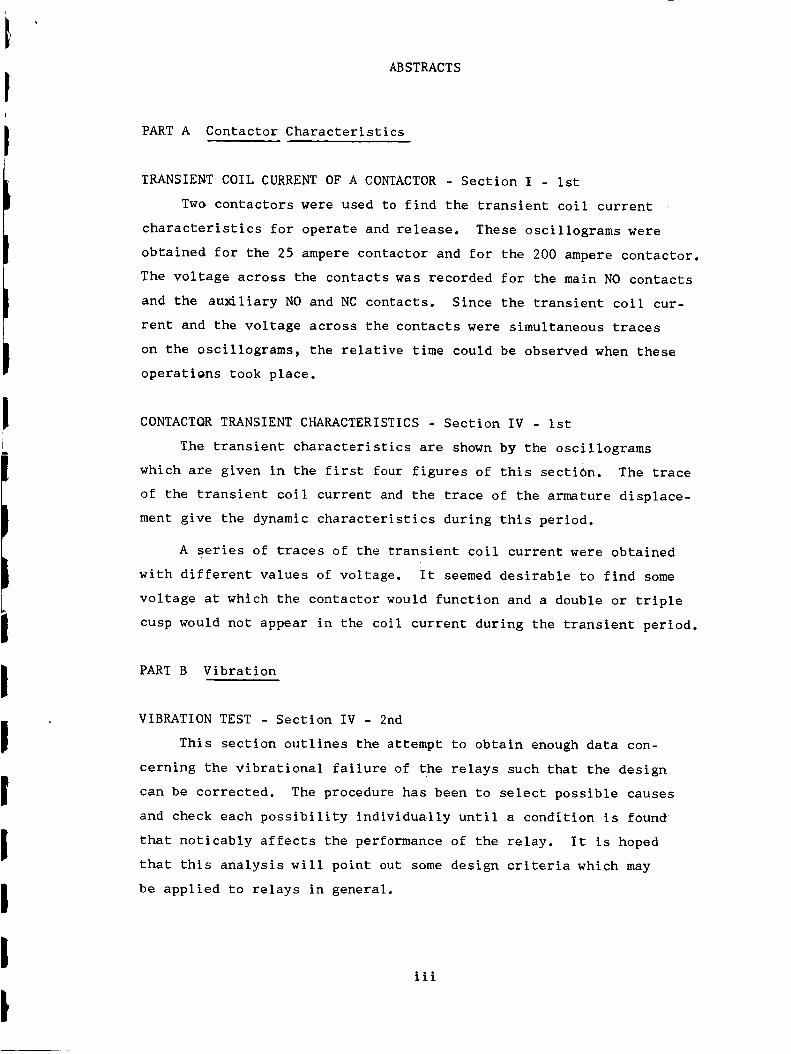
ABSTRACTS

PARTA Contactor Characteristics

TRANSIENT COIL CURRENT OF A CONTACTOR - Section I - ist

Two contactors were used to find the transient coil current

characteristics for operate and release. These oscillograms were

obtained for the 25 ampere contactor and for the 200 ampere contactor.

The voltage across the contacts was recorded for the main NO contacts

and the au_liary NO and NC contacts. Since the transient coil cur-

rent and the voltage across the contacts were simultaneous traces

on the oscillograms, the relative time could be observed when these

operations took place.

CONTACTOR TRANSIENT CHARACTERISTICS - Section IV ist

The transient characteristics are shown by the oscillograms

which are given in the first four figures of this section. The trace

of the transient coil current and the trace of the armature displace-

ment give the dynamic characteristics during this period.

A series of traces of the transient coil current were obtained

with different values of voltage. It seemed desirable to find some

voltage at which the contactor would function and a double or triple

cusp would not appear in the coil current during the transient period.

PART B Vibration

VIBRATION TEST - Section IV - 2nd

This section outlines the attempt to obtain enough data con-

cerning the Vibrational failure of the relays such that the design

can be corrected. The procedure has been to select possible causes

and check each possibility individually until a condition is found

that noticably affects the performance of the relay. It is hoped

that this analysis will point out some design criteria which may

be applied to relays in general.

iii

VIBRATION TEST CONTINUED - Section II - 3rd

The problem of failure of the relay, for the purpose of this

discussion shall be defined as a separating of the contacts when the

coil is energized= The contact system was considered and five pos-

sible causes of failure defined. Of these five one had been investi-

gated previously, one was discarded as unlikely, and one was investi-

gated in some detail. This report is concerned with the motion of

the movable contact bar with respect to the armature shaft. The

spring tension was varied and the effects noted.

PART C Contact Study

PRELIMINARY INFESTIGATION AND PROPOSAL OF RELAY CONTACT DESIGN - Section III

In this preliminary study, three areas are discussed, which

relate to design. Design terminology as applied to devices in general

with some definitions is given The second part deals with the

electrical contact system in particular. Whereas, the third part

is concerned with an attempt to work out a scheme which can be applied

to an electric contact system with given load requirements.

Ist

q

CONTACT RATING - Section II - 2nd

This discussion is an attempt to furnish a partial answer to

the question, "What are the actual load conditions to which a con-

tactor is subjected?" An outline is made of one analysis of the

problem. No doubt, this study should be extended.

THEORETICAL INVESTIGATION AND SOME EXPERIMENTAL DATA FOR ELECTRICAL

CONTACT FAILURE CAUSED BY ELECTRICAL LOADING Section III - 2nd

This section is a preliminary attempt to find analytical re-

lationships with which to predict the life of a contactor contact

system with respect to electrical load with a given degree of cer-

tainty. The degree of certainty is expressed as a probability for

the number of contactors of interest which are expected to meet the

predicted life The life is expressed in terms of number of oper-

ations based on a given electrical load condition, This was ob-

tained from more basic considerations involving the two relationships;

;_v

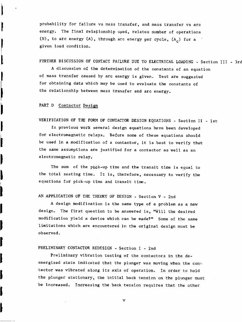
probability for failure vs mass transfer, and mass transfer vs arc

energy. The final relationship u_ed, relates number of operations

(N), to arc energy (A), through arc energy per cycle, (Ac) for a

given load condition.

FURTHER DISCUSSION OF CONTACT FAILURE DUE TO ELECTRICAL LOADING - Section III - 3rd

A discussion of the determination of the constants of an equation

of mass transfer caused by arc energy is given. Test are suggested

for obtaining data which may be used to evaluate the constants of

the relationship between mass transfer and arc energy.

PART D Contactor Design

VERIFICATION OF THE FORM OF CONTACTOR DESIGN EQUATIONS - Section II - ist

In previous work several design equations have been developed

for electromagnetic relays. Before some of these equations should

be used in a modification of a contactor, it is best to verify that

the same assumptions are justified for a contactor as well as an

electromagnetic relay.

The sum of the pgck-up time and the transit time is equal to

the total seating time. It is, therefore, necessary to verify the

equations for pick-up time and transit time.

AN APPLICATION OF THE THEORY OF DESIGN - Section V - 2nd

A design modification is the same type of a problem as a new

design. The first question to be answered is, "Will the desired

modification yield a device which can be made?" Some of the same

limitations which are encountered in the original design must be

observed.

PRELIMINARY CONTACTOR REDESIGN - Section I - 2nd

Preliminary vibration testing of the contactors in the de-

energized state indicated that the plunger was moving when the con_

tactor was vibrated along its axis of operation° In order to hold

the plunger stationary, the initial back tension on the plunger must

be increased. Increasing the back tension requires that the other

v

eontactor parameters be changed. Two possible combinations of fixed

parameters were selected and the other parameters computed, The pro-

cedure used to take the parameters specified and list them on the

design matrix is given, Since the numerical data about the values

of the parameters existing on the given contactor were not known,

the changes are given in terms of percent.

CONTINUATION OF PRELIMINARY CONTACTOR REDESIGN - Section I 3rd

It appears that some combination of increased coil power and

coil length might be the most feasible in the redesign of the conM

tactor. Additional calculations are given in this section to

show the result of increasing the hack tension by a combination of

coil power and coil length. Several parameters are plotted against

coil power

vi

CONCLUSIONS

PART A Contactor Characteristics

TRANSIENT COIL CURRENT OF A CONTACTOR - Section I - Ist

The two contactors which were studied by means of obtaining the

transient coil current and voltage across the contacts characteris-

tics showed one common trait. There was a double hump immediately

after the first cusp of the current build-up trace. The conclusion

was that an obstruction such as the picking-up of an additional spring

caused this hesitation in the motion of the armature.

CONTACTOR TRANSIENT CHARACTERISTICS - Section IV - ist

It was assumed that the transient characteristics of contactors

would be similar to the transient characteristics of relays. The

oscillograms which were obtained for this section demonstrate that

this assumption is correct. The first four oscillograms show that

the transient current trace has irregularities in it which correspond

to the trace of the instanteous position of the armature and that

there was a hesitation of the armature during its travel.

The last two oscillograms prove that the armature hesitation

may be suppressed by increasing the impressed voltage on the coil.

It is believed that the armature hesitation causes unsatisfactory

functioning of the contactor.

PART B Vibration

VIBRATION TEST - Section IV - 2nd

The investigation to date has dealt with the armature and the

contact mountings° The armature, although appearing to have some

type of motion relative to the coil, does not seem to have much

effect on the failure of the contacts when the relay is energized.

The mountings of the stationary contacts have some effect, although

the conclusions to this part of the test are not yet complete. The

mountings of the movable contacts have a much greater effect on the

vii

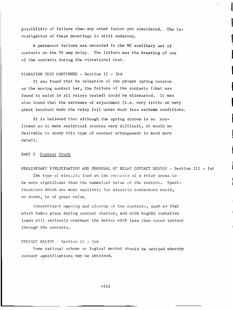
possibility of failure than any other factor yet considered. The in-

vestigation of these mountings is still underway.

A permanent failure was detected in the NC auxiliary set of

contacts on the 50 amp relay_ The failure was the breaking of one

of the contacts during the vibrational test_

VIBRATION TEST CONTINUED - Section II - 3rd

It was found that be selection of the proper spring tension

on the moving contact bar, the failure of the contacts (that was

found to exist in all relays tested) could be eliminated. It was

also found that the extremes of adjustment (i.e. very little or very

great tension) made the relay fail under much less extreme conditions.

It is believed that although the spring system is so non-

linear as to make analytical studies very difficult, it would be

desirable to study this type of contact arrangement in much more

detail.

PART C Contact Study

PRELIMINARY INVESTIGATION AND PROPOSAL OF RELAY CONTACT DESIGN - Section III - ist

The type of elee5_ic load on the contacts of a relay seems to

be more significant than the numerical value of the current. Speci-

fications which are more realistic for electric contactors would,

no doubt, be of great va]ue,_

Intermittent opening and closing of the contacts, such as that

which takes place during contact chatter, and with highly inductive

loads will seriously overheat the device with less than rated current

through the contacts.

CONTACT RATING Section II - 2nd

Some rational scheme or logical method should be devised whereby

contact specifications may be obtained.

viii

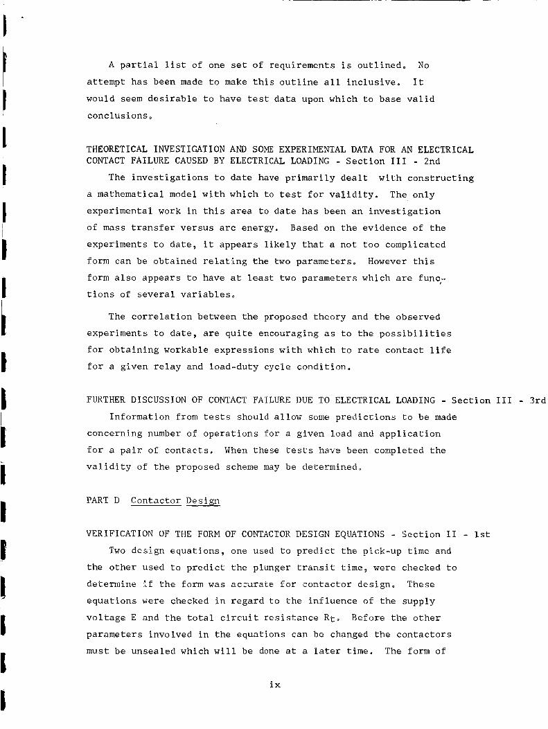
A partial list of one set of requirements is outlined. No

attempt has been made to make this outline all inclusive° It

would seem desirable to have test data upon which to base valid

conclusions°

THEORETICAL INVESTIGATION AND SOME EXPERIMENTAL DATA FOR AN ELECTRICAL

CONTACT FAILURE CAUSED BY ELECTRICAL LOADING - Section III 2nd

The investigations to date have primarily dealt with constructing

a mathematical model with which to test for validity. The only

experimental work in this area to date has been an investigation

of mass transfer versus arc energy. Based on the evidence of the

experiments to date, it appears likely that a not too complicated

form can be obtained relating the two parameters° However this

form also appears to have at least two parameters which are func_

tions of several variables°

The correlation between the proposed theory and the observed

experiments to date, are quite encouraging as to the possibilities

for obtaining workable expressions with which to rate contact life

for a given relay and load-duty cycle condition°

FURTHER DISCUSSION OF CONTACT FAILURE DUE TO ELECTRICAL LOADING - Section III - 3rd

Information from tests should allow some predictions to be made

concerning number of operations for a given load and application

for a pair of contacts° When these tests have been completed the

validity of the proposed scheme may be determined°

PART D Contactor Design

VERIFICATION OF THE FORM OF CONTACTOR DESIGN EQUATIONS - Section II - Ist

Two design equations, one used to predict the pick=up time and

the other used to predict the plunger transit time, were checked to

determine if the form was accurate for contactor design° These

equations were checked in regard to the influence of the supply

voltage E and the total circuit resistance Rto Before the other

parameters involved in the equations can be changed the contactors

must be unsealed which will be done at a later time. The form of

ix

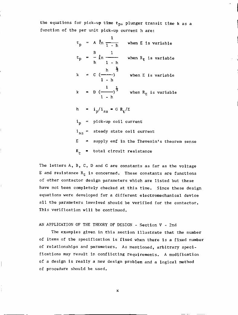
the equations for pick-up time tp, plunger transit time k as afunction of the per unit pick-up current h are:

itp = A _n i---'-_ when E is variable

tpB i

h i - h

h= c(--)

1 - h

when R t is variable

when E is variable

i l

= D (--) 3

1 - hwhen R t is variable

h

iP

iSS

Rt

ip/iss = G Rt/E

= pick-up coil current

= steady state coil current

= supply emf in the Thevenin's theorem sense

= total circuit resistance

The letters A, B, C, D and G are constants as far as the voltage

E and resistance R t is concerned. These constants are functions

of other contactor design parameters which are listed but these

have not been completely checked at this time. Since these design

equations were developed for a different electromechanical device

all the parameters involved should be verified for the contactor.

This verification will be continued.

AN APPLICATION OF THE THEORY OF DESIGN Section V - 2nd

The examples given in this section illustrate that the number

of items of the specification is fixed when there is a fixed number

of relationships and parameters. As mentioned, arbitrary specl-

fications may result in conflicting requirements. A modification

of a design is really a new design problem and a logical method

of procedure should be used.

X

PRELIMINARY CONTACTOR REDESIGN - Section I - 2nd

The results of the preliminary redesign points out the fact

that only a certain number of parameters can be fixed or changed.

If a given mechanical arrangement of the elements is to be used

then the parameters which determine this must be fixed° These

fixed parameters along with the ones being changed are limited

to 8 in number.

When the coil dimensions are fixed, among other things, the

coil power must increase in order to increase the back tension.

In this case the coil power required increased directly with the

back tension° However, this depends upon the parameters that are

selected° Since heat dissipation was not known, the redesign re-

suiting in an increase in coil power may be undesirable° A second

computation was made with the coil power fixed and the coil length

variable° The results of this computation indicated that the coil

length must increase directly with the increase in back tension.

These results show that an increase in the mechanical work per-

formed by the contactor must be accompanied by an increase in coil

power or an increase in coil volume or a combination of both°

CONTINUATION OF PRELIMINARY CONTACTOR REDESIGN - Section I - 3rd

Increasing the back tension, Po, on the plunger in order to

raise the G level requires certain changes in the other parameters.

For the set of specified parameters used, which contain P, N , E,

M 9 Rs9 xo and _A, it is shown that the product of the coll power

P and the coil length % is directly proportional to Po o The in-

fluence on the unspecified parameters of changing the coil power

is shown by a set of curves for various values of the factor _ .

The factor @ is the ratio of the core diameter to the outside

coil diameter. A value of _ which will minimize the coil length

for a given value of coil power is obtained° In addition, the

influence of the coil bobbin insulation is presented by comparison

of the curves in the figures. For the contactor considered, an

increase in coil efficiency of approximately 50% can be obtained

by changing the core diameter and the bobbin insulation thickness°

xi

SCOPEOFWORK

The work will consist of the following:

(a) Review several contactor designs presently employed

for space vehicle applications and select the most

promising designs for further analysis.

(b) Analyze in detail the design to determine the para-

meters w_hichare not consistent with the requirements.

(c) Propose a modified design which would more nearly

satisfy the required performance.

(d) The design performance of the contactor is as follows:

(I) Withstand 20g or more vibration with a

frequency range of i0 to 2000 cps.(2) That the contactor have a minimumlife of

I0,000 operations at rated load.(3) Temperature limits - 65° to + 125°F.

(4) Contactor shall be contained in a hermetically

sealed package.

(e) Evaluate modified design unit.

xii

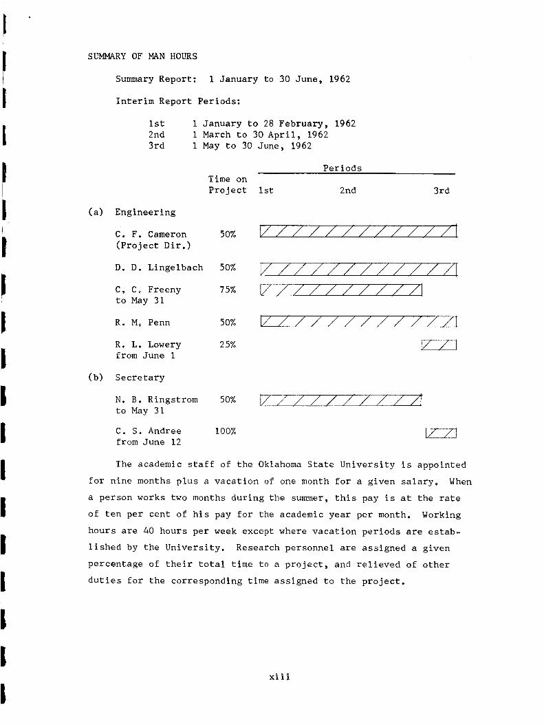
SUMMARYOFMANHOURS

SummaryReport: 1 January to 30 June, 1962

Interim Report Periods:

Ist i January to 28 February, 19622nd i March to 30 April, 19623rd I Mayto 30 June, 1962

PeriodsTime onProject Ist 2nd

(a) Engineering

C. F. Cameron(Project Dir.)

D. D. Lingelbach 50%

C, C. Freeny 75%to May31

R. M_Penn 50%

R_ L. Lowery 25%from June I

(b) Secretary

N. B. Ringstromto May31

C. S. Andree 100%from June 12

3rd

50% V / / / ////////

V///////////I

V-7////////l

V //////// ///I

50% V--V7//////,'1

The academic staff of the Oklahoma State University is appointed

for nine months plus a vacation of one month for a given salary° When

a person works two months during the summer, this pay is at the rate

of ten per cent of his pay for the academic year per month. Working

hours are 40 hours per week except where vacation periods are estab-

lished by the University. Research personnel are assigned a given

percentage of their total time to a project, and relieved of other

duties for the corresponding time assigned to the project.

xiii

I

II

I

iI

I

I

I

I

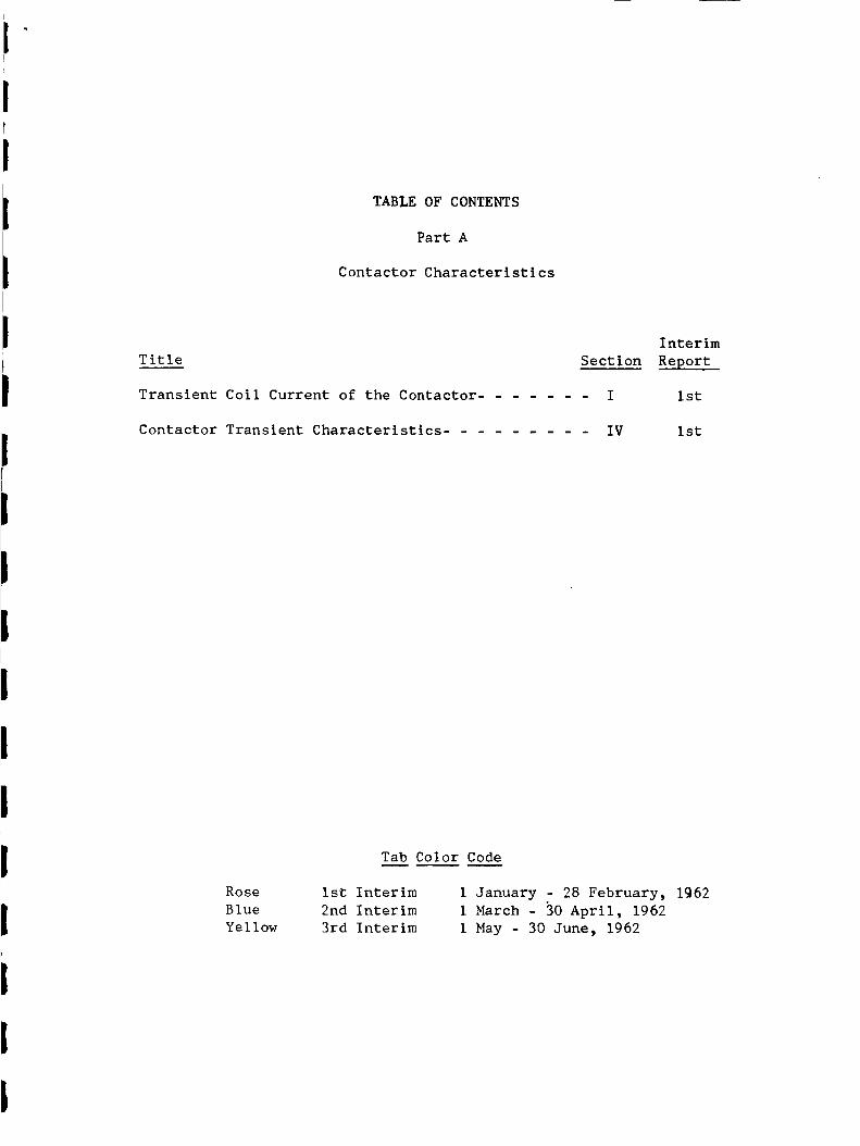
TABLE OF CONTENTS

Part A

Contactor Characteristics

Title

Transient Coil Current of the Contactor- - -

Interim

Section Report

I Ist

Contactor Transient Characteristics ......... IV Ist

Rose

Blue

Yellow

Tab Color Code

Ist Interim I January - 28 February, Ig62

2nd Interim i March - i0 April_ 1962

3rd Interim i May - 30 June, 1962

SECTION I

TRA_SIENT COIL CURRENT OF A CONTACTOR

Much may be learned about the behavior of an electrical contactor or

a heavy duty relay by observing the transient coll current and the voltage

across the contacts. These traces may be recorded by a Camera attached

to a dual beam oscilloscope. Since the two beams of the oscilloscope give

a record of events which have taken place simultaneously, this scheme may

be used to analyze the sequence of events in a device such as a contactor.

The figure which is included herewith shows a typical set of transient

characteristics for a relay. In this study, relay and contactor will be

used interchangeably. It might be said that a contactor is a heavy duty

relay. In the figure the time scale is on the horizontal axis and the

vertical axis may be used to represent current, voltage, position or some

other quantity. _vo of these quantities may be recorded simultaneously

as a function of time. Since the time is the same for each trace at some

particular point on the horizontal axis, these oscillograms are an excel-

lent means of explaining the happenings in such a device as a contactor.

The trace which is labeled "A" in the illustrative diagram shows the

instantaneous current for a time interval of zero time to steady-state

current conditions, which may be fifty or one hundred milliseconds later.

It is to be noted that there is a very pronounced cusp in this current

trace. The sharp tip of the cusp indicates the time at which the armature

has completed its travel. Curve "B" is a trace which indicates the in-

stantaneous position of the armature. In this diagram, the coil is

energized at zero time and the armature was in the open position. The

armature has closed at time (t:) which coincides with the sharp point on

the current cusp.

statement.

Numerous oscillograms have proved the validity of this

l- I

Voltage Across Contacts

NCContacts0

Arm Position

NOContacts

S

Time of Overtravel

0 t, t, t,Time

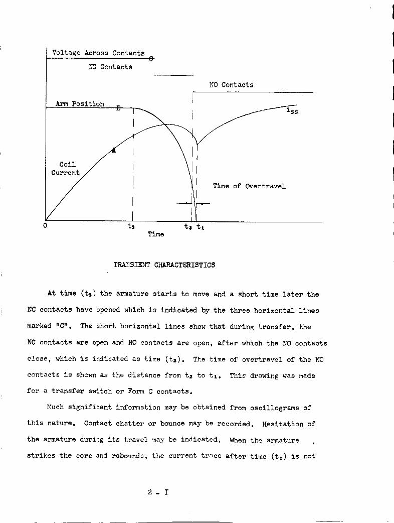
TRANSIENT CHARACTERISTICS

At time (t3) the armature starts to move and a short time later the

NC contacts have opened which is indicated by the three horizontal lines

marked "C". The short horizontal lines show that during transfer, the

NC contacts are open and NO contacts are open, after which the NO contacts

close, which is indicated as time (t,). The time of overtravel of the NO

contacts is shown as the distance from tz to t,. Thi_ drawing was made

for a transfer switch or Form C contacts.

Much significant information may be obtained from oscillograms of

this nature. Contact chatter or bounce may be recorded. Hesitation of

the armature during its travel may be indicated. When the armature

strikes the core and rebounds, the current trace after time (t,) is not

2- I

I

i

II

I

I

I

L

a smooth curve. The height of the current trace before the cusp compared

to the steady.state value of current gives an idea of the stability of

the device. The steady-state current is indicated as iss. Operate time

is the time from zero to t,.

Under release conditions, the transient current may be recorded as

well as the voltage across the contacts. These release traces also have

certain general characteristics. These curves or traces for operate and

release may be regarded as the transient characteristics.

Each relay design type will exhibit certain peculiarities which are

common to that particular design type. Any variation in these character.

istlcs indicates that some abnormal situation has arisen.

The oscillograms shown in Figures 1 through 12 were made in order to

have a record of the transient characteristic of each of the contactors

received. If during testing of the contactors any changes occur, a com-

parison can be made by recording the transient characteristics after test-

ing and comparing them with the original oscillograms. These oscillograms

are recorded at some particular voltage, usually the rated voltage. How-f

ever, additional information can be obtained by recording the transients at

different values of voltage.

Figure I shows simultaneously the coil current build.up and the con-

tact voltage across the power contacts LI-TI of the 25 ampere contactor

#l. Since the power contacts are a NO pair, the contactor voltage trace

has only two levels. Comparison of the coil current trace and the contact

voltage trace shows that the power contacts function at the first cusp.

Or in other words, the functioning of the power contacts in this case seems

to cause the first cusp.

Figure 2 shows the contact voltage across the NO contacts of the

auxiliary set and the coil current build-up. The breaks in the contact

3-I

vol_age trace (a) indicates contact bounce which continues for somelittle

time. For inductive loads this could be a very unsatisfactory situation.

The oscillogram of Figure 3 gives the transient coil current and

the voltage across the NC auxiliary contacts. In all of the traces for

the current build-up in the first three oscillograms, the current shows

three different cusps, however the last one is rather minor.

The transients during the release period are shownin Figures 4, 5

and 6. The Figure 4 shows the decay of the coil current and the opening

of the NOcontacts for the 25 ampere contactor. The humpon the current

decay trace has a saddle. This seemsto be a characteristic of this

particular contactor. At the moment, no opinion has been formed as to

why this particular shape exists. Figures 5 and 6 are somewhatsimilar

to Figure _.

Oscillograms which are given in Figures 7, 8, 9, I0, II and 12 are

those obtained on the 200 ampere contactor. The transient current trace

has a double humpbut thedecay trace is somewhatdifferent than that of

the 25 amperecontactor.

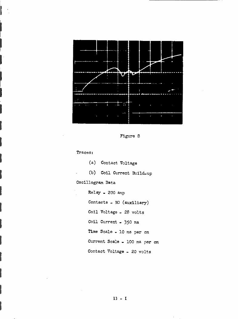
The voltage across the auxiliary contacts of Figure 8 shows some

contact bounce. The other figures do not give muchevidence of bounce.

Figures 7, 8 and 9 are the transients for operate conditions and Figures

I0, II, and 12 are for release conditions.

These oscillograms give someideas about the functioning of the

contactor. Below each oscillogram is given the various conditions which

were imposed on that device.

It is evident that muchmorewill have to be learned about these

cdntactors before specific recommendationscan be madefor improvement.

It seemsevident, however, that the armature hesitation for operation

4-I

conditions will bear further investigation. It is planned to continue

with this idea in an attempt to cause the armature to movedirectly from

the open position to the closed position when the coll is energized.

I

I

I

I

I

I

I

I

I

I

I

i 5- I

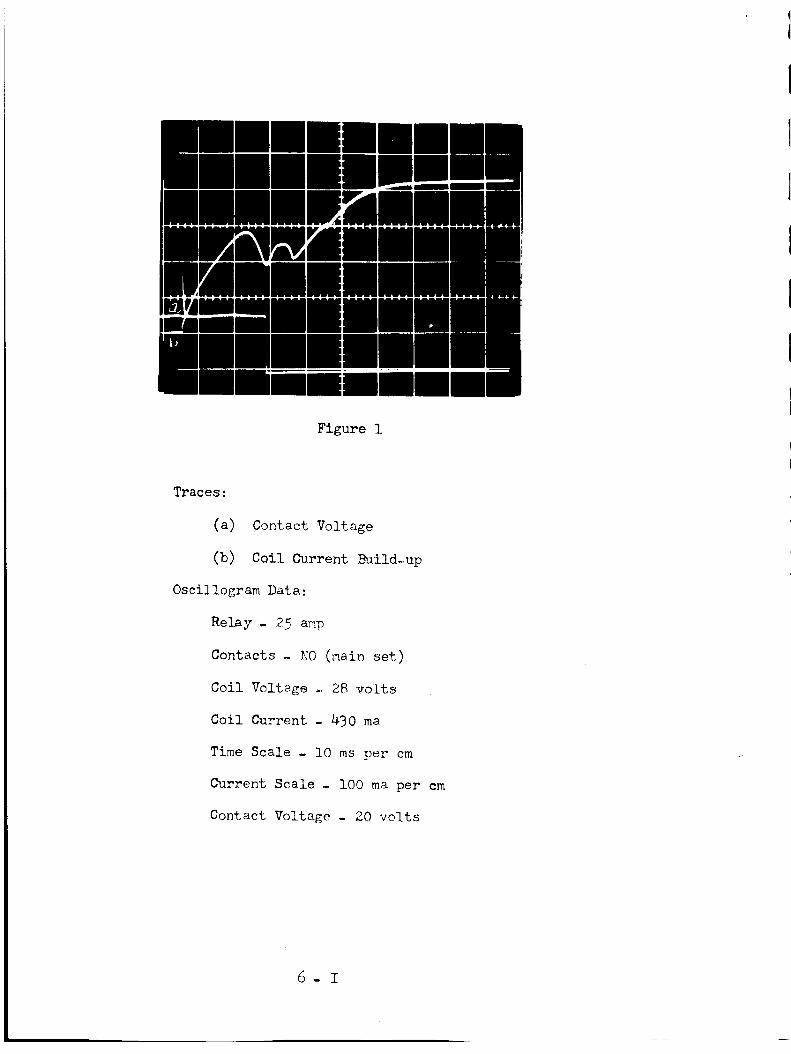
Figure 1

Traces:

(a) Contact Voltage

(b) Coil Current Build-up

Oscillogram Data:

Relay . 2_ azp

Contacts o NO (maio set)

Coil Voltage - 28 volts

Coil Current - 430 ma

Time Scale - I0 ms per cm

Current Scale -i00 ma per cm

Contact Voltage - 20 volts

6- I

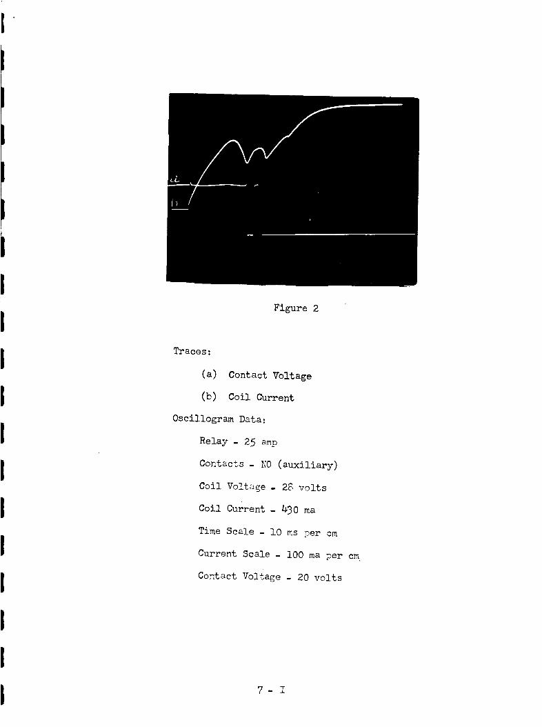
Figure 2

Traces:

(a) Contact Voltage

(b) Coil Current

Oscillogram Data:

Relay - 25 a_,p

Contacts - NO (auxiliary)


Coil current - 430 ma

Time Scale - lO ms per cm

Current Scale - lO0 ma per cm


7- I

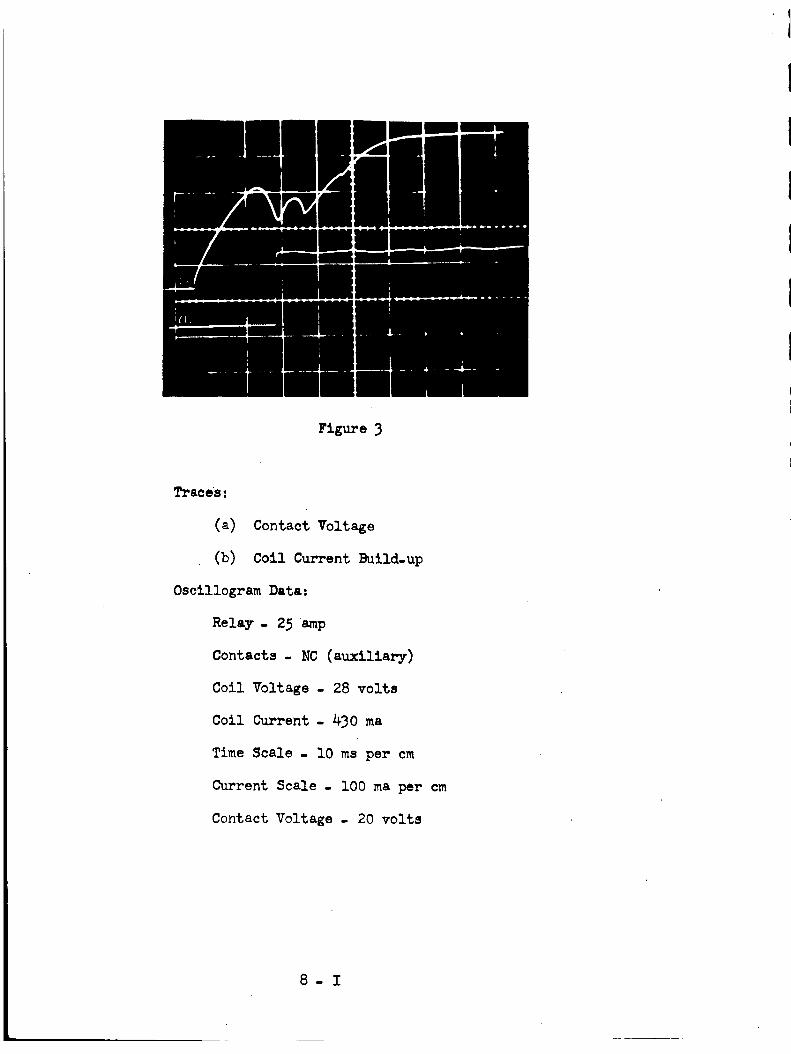
Figure 3

Traces:

(a)

(b)

Contact Voltage

Coil Current Build.up

Oscillogram Data:

Relay. 25 amp

Contacts - NC (auxiliary)

Coil Voltage . 28 volts



Current Scale . I00 ma per cm

Contact Voltage . 20 volts

8-1

Figure

Traces:

(a) Contact Voltage

(b) Coil Current Decay

Oscillogram Data:

Relay - 25 amp

Contacts - NO (main set)




Current Scale - I00 ma per cm


Coil Dischsrge Path - diode

9- I

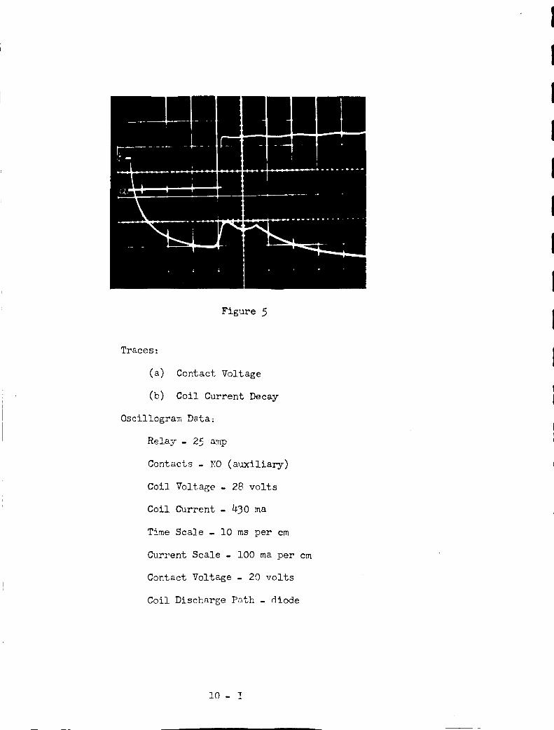
Figure 5

Traces:

(a) Contact Voltage


Oscillogram Data_

Relay . 25 amp





Current Scale - lO0 ma per cz


Coil Discharge Path . _iode

I0- I

Figure 6

Traces:

(a) Contact Voltage


0scillogram Data:

Relay - 25 amp


Coil Voltage - 2S volts





Coil Discharge Path - diode

II- I

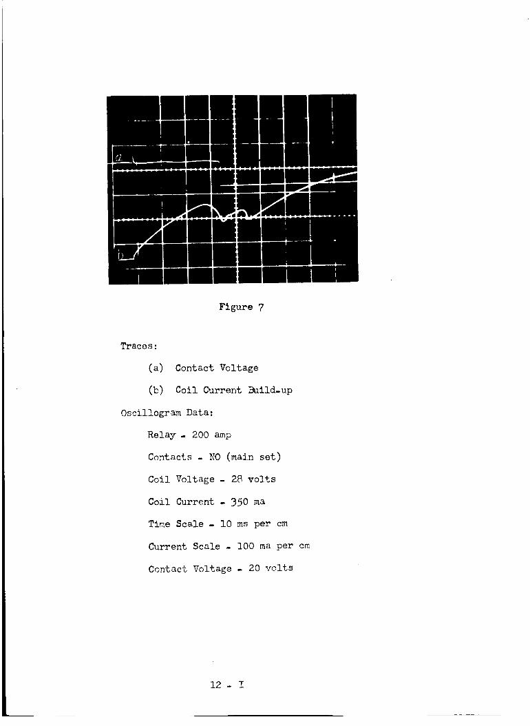
Figure 7

Traces:

(a)

(b)

Contact Voltage

Coil Current Build-up

Osci!!ogram Data:

Relay- 200 amp







12- I

I

I

l

I

I

I

l

I

I

I

I

I

i

Figure 8

Traces:

(a) Contact Voltage

(b) Coil Current Build-up

Oscillogram Data

Relay- 200 amp




Time Scale - l0 ms per cm

Current Scale - 100 ma per cm


13 - I

Figure 9

Traces:

(a)

(b)

Contact Voltage


Oscillogram Data:

Relay - 200 amp







14- I

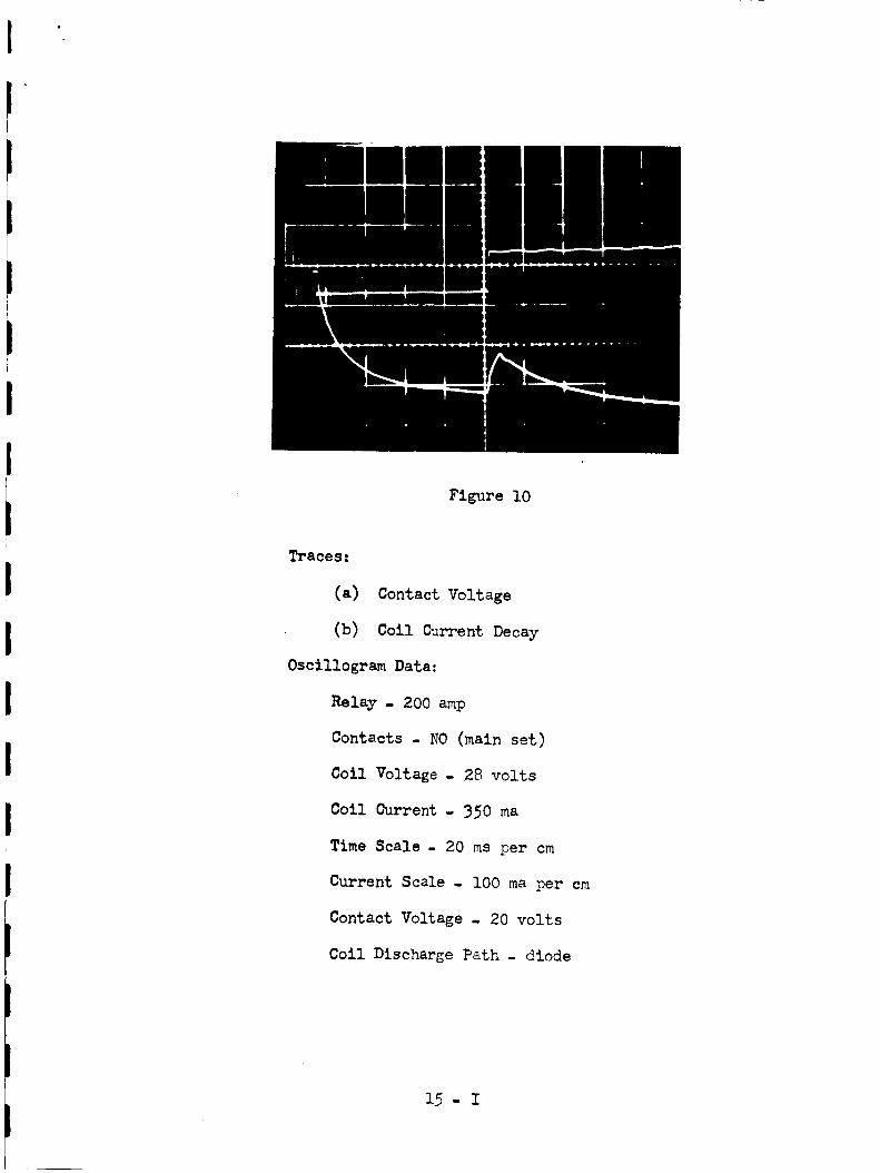
Figure l0

rraces_

(a) Contact Voltage


0scillogram Data:

Relay . 200 azp




Time Scale - 20 ms per cm



Coil Discharge P_th - diode

15 - I

Figure ll

Traces:

(a)

(b)

Contact Voltage

Coll Current Decay

Oscillogram Data:

Relay - 200 amp


Coil Voltage . 28 volts





Coil DischarGe Paths - diode

16- I

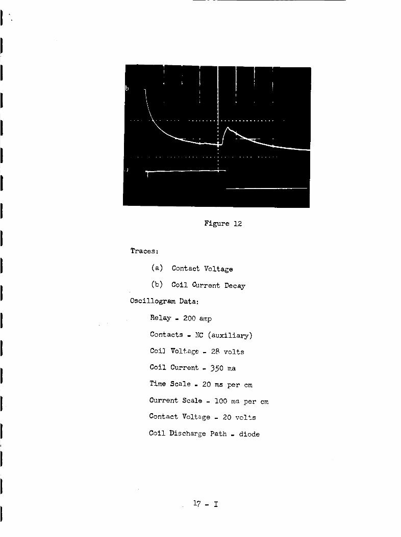
Figure 12

Traces:

(a) Contact Voltage


Oscillogram Data:

Relay - 200 amp


Coi_ Voltage . 28 volts



Current Scale - I00 maper cm


Coil Discharge Path - diode

17 - I

I

I

I

I

I

I

I

I

I

I

I

R

I

I

l

I

i

i

i

SECTION IV

CONTACTOR TRANSIENT CHARACTERISTICS

In the design of relays it is sometimes desirable to mount the

movable contact (of a normally open set of contacts) such that it will

touch the fixed contact before the armature has completed its travel.

It is possible that this design, under extreme operating conditions,

could lead to a premature failure of the relay.

Failure of the type relay being discussed in this report is defined

to be an opening of the contacts, the open time exceeding I0"_ seconds,

during the period of time when they are intended to be closed.

It is desired that the relay carry the rated current and undergo

vibrations up to 20 times the force of gravity at frequencies of I0 to

2000 cps. In the steady state operated condition, the contacts are held

together by a force which for the purpose of this discussion we will

define as the maximum force. When this force exists on the contacts,

the cor_act surfaces will be termed, "under maximum pressure."

A direct Cause of failure could be the opening of the contacts due

to the forces induced by vibrations. To minimize the probability of

this type of failure, it is obvious that maximum pressure is required at

all times when the contacts are closed.

An indirect cause of failure could be the deterioration of the

contacts themselves caused by overheating and arcing. Neglecting the arc

energy, the temperature of the contacts is, among other things, a function

of the ISR loss in the contacts. The contact resistance is a function of

the pressure on the contact surfaces, an increase in pressure results in

a decrease in resistance.

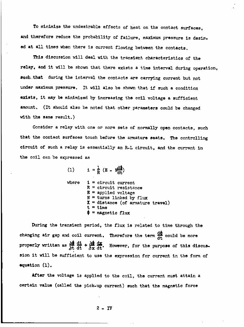
To minimize the undesirable effects of heat on the contact surfaces,

and therefore reduce the probability of failure, maximumpressure is desir-

ed at all times whenthere is current flowing between the contacts.

This discussion will deal with the transient characteristics of the

relay, and it will be shownthat there exists a time interval during operation,

such.that during the interval the contacts are carrying current but not

under maximumpressure. It will also be shown that if such a condition

exists, it may be minimized by increasing the coil voltage a sufficient

amount. (It should also be noted that other parameters could be changed

with the same result. )

Consider a relay with one or more sets of normally open contacts, such

that the contact surfaces touch before the armature seats. The controlling

circuit of such a relay is essentially an R-L circuit, and the current in

the coil can be expressed as

(I)

where i = circuit current

R = circuit resistance

E = applied voltage

N = turns linked by flux

X = distance (of armature travel)t = time

$ = magnetic flux

During the transient period, the flux is related to time through the

changing air gap and coil current. Therefore the term _ could be more

properly written as _ di + _ _x However, for the purpose of this discus-_t dt _x dr"

sion it will be sufficient to use the expression for current in the form of

equation (i).

After the voltage is applied to the coil, the current must attain a

certain value (called the pick-up current) such that the magnetic force

2-IV

I

I

i

I

I

I

I

L

i

I

I

I

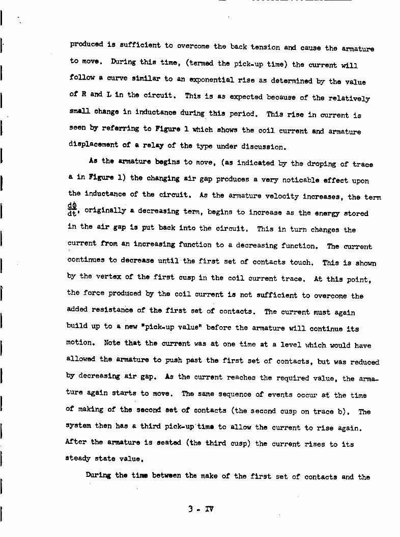
produced is sufficient to overcome the back tension and cause the armature

to move. During this time, (termed the pick-up time) the current will

follow a curve similar to an exponential rise as determined by the value

of R and L in the circuit. This is as expected because of the relatively

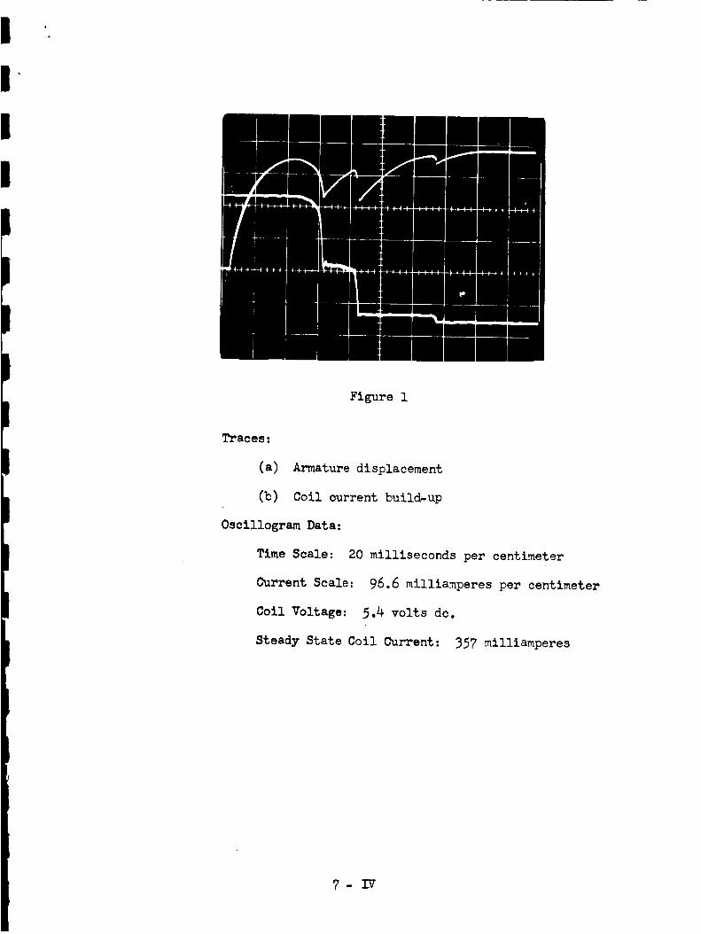
small change in inductance during this period. This rise in current is

seen by referring to Figure I which shows the coil current and armature

displacement of a relay of the type under discussion.

As the armature begins to move, (as indicated by the droping of trace

a in Figure i) the changing air gap produces a very noticable effect upon

the inductance of the circuit. As the armature velocity increases, the term

d__ originally a decreasing term, begins to increase as the energy storeddr'

in the air gap is put back into the circuit. This in turn changes the

current from an increasing function to a decreasing function. The current

continues to decrease untilthe first set of contacts touch. This is shown

by the vertex of the first cusp in the coil current trace. At this point,

the force produced by the coil current is not sufficient to overcome the

added resistance of the first set of contacts. The current must again

build up to a new "plck-up value" before the armature will continue its

motion. Note that the current was at one time at a level _ich would have

allowed the armature to push past the first set of contacts, but was reduced

by decreasing air gap. As the current reaches the required value, the arma-

ture again starts to move. The same sequence of events occur at the time

of making of the second set of contacts (the second cusp on trace b). The

system then has a third pick-up'time to allow the current to rise again.

After the armature is seated (the third cusp) the current rises to its

steady state value.

During the time between the make of the first set of contacts and the

3-1V

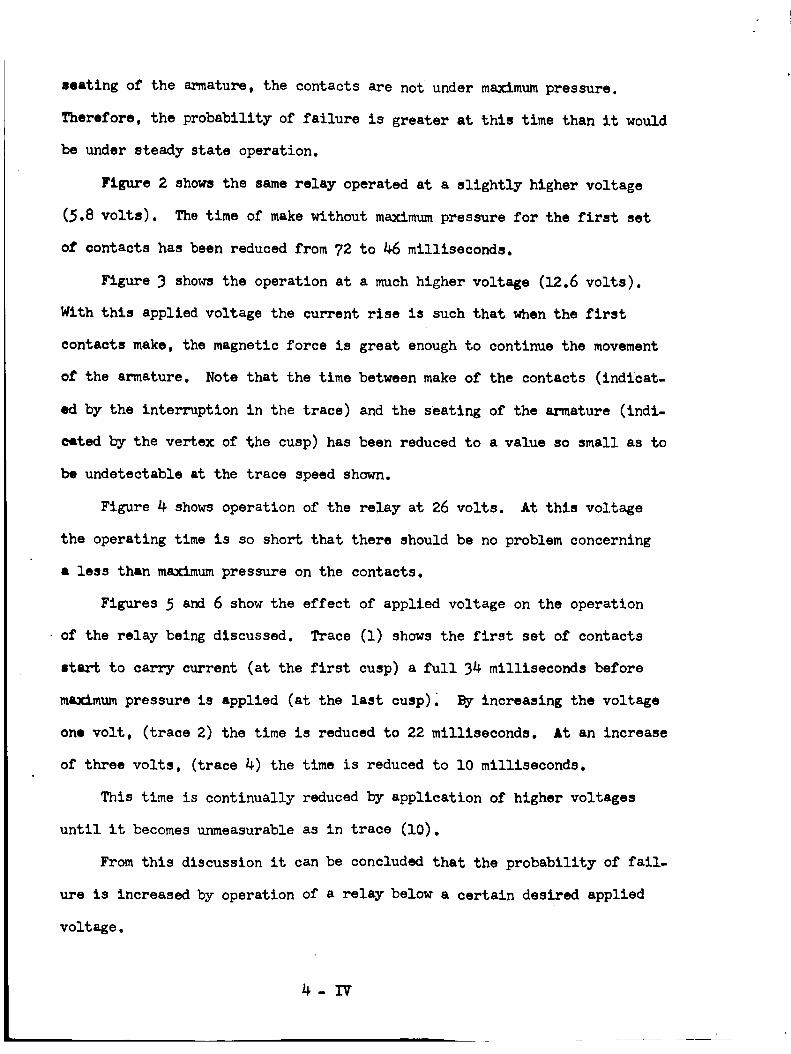
seating of the armature, the contacts are not under maximum pressure.

Therefore, the probability of failure is greater at this time than it would

be under steady state operation.

Figure 2 shews the same relay operated at a sllghtlyhigher voltage

(5.8 volts). The time of make without maximum pressure for the first set

of contacts has been reduced from 72 to 46 milliseconds.

Figure 3 shows the operation at a much higher voltage (12.6 volts).

With this applied voltage the current rise is such that when the first

contacts make, the magnetic force is great enough to continue the movement

of the armature. Note that the time between make of the contacts (indicat-

ed by the interruption in the trace) and the seating of the armature (indi-

cated by the vertex of the cusp) has been reduced to a value so small as to

be undetectable at the trace speed shown.

Figure 4 shows operation of the relay at 26 volts. At this voltage

the operating time is so short that there should be no problem concerning

a less than maximum pressure on the contacts.

Figures 5 and 6 show the effect of applied voltage on the operation

• of the relay being discussed. Trace (1) shows the first set of contacts

start to carry current (at the first cusp) a full 3_ milliseconds before

maximum pressure is applied (at the last cusp). By increasing the voltage

one volt, (trace 2) the time is reduced to 22 milliseconds. At an increase

of three volts, (trace 4) the time is reduced to I0 milliseconds.

This time is continually reduced by application of higher voltages

until it becomes unmeasurable as in trace (i0).

From this discussion it can be concluded that the probability of fail-

ure is increased by operation of a relay below a certain desired applied

voltage.

_-IV

I

I

i

I

I

II

I

I

iI

II

I

I

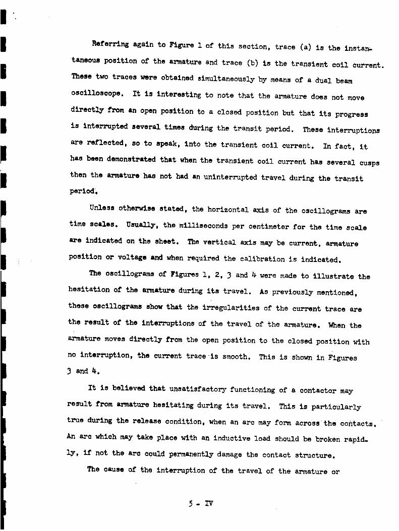
Referring again to Figure i of this section, trace (a) is the instan-

taneous position of the armature and trace (b) is the transient coil current.

These two traces were obtained simultaneously by means of a dual beam

oscilloscope. It is interesting to note that the armature doesnot move

directly from an open position to a closed position but that its progress

is interrupted several times during the transit period. These interruptions

are reflected, so to speak, into the transient coil current. In fact, it

has been demonstrated that when the transient coil current has several cusps

then the armature has not had an uninterrupted travel during the transit

period.

Unless otherwise stated, the horizontal axis of the oscillograms are

time scales. Usually, the milliseconds per centimeter for the time scale

are indicated on the sheet. The vertical axis maybe current, armature

position or voltage and when required the calibration is indicated.

The oscillograms of Figures I, 2, 3 and 4were made to illustrate the

hesitation of the armature during its travel. As previously mentioned,

these oscillograms show that the irregularities of the current trace are

the result of the interruptions of the travel of the armature. When the

armature moves directly from the open position to the closed position with

no interruption, the current trace is smooth. This is shown in Figures

3 andS.

It is believe_Ithat unsatisfactory functioning of a contactor may

result from armature hesitating during its travel. This is particularly

true during the release condition, when an arc may form across the contacts.

An arc which may take place with an inductive load should be broken rapid.

ly, if not the arc could permanently damage the contact structure.

The cause of the interruption of the travel of the armature or

5-1V

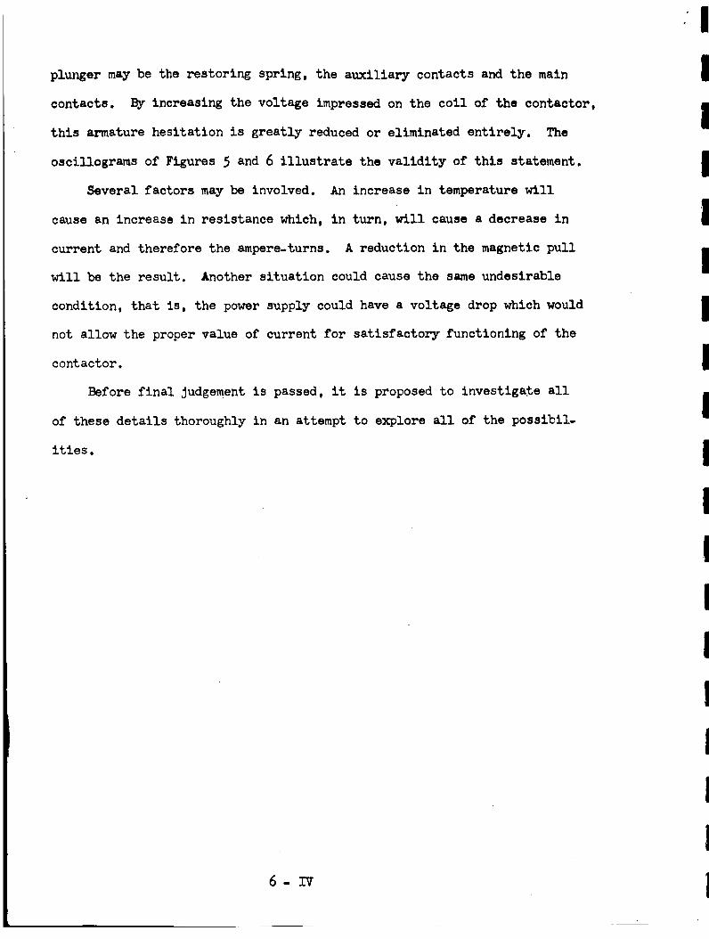
plunger maybe the restoring spring, the auxiliary contacts and the main

contacts. By increasing the voltage impressed on the coil of the contactor,

this armature hesitation is greatly reduced or eliminated entirely. The

oscillograms of Figures 5 and 6 illustrate the validity of this statement.

Several factors maybe involved. An increase in temperature will

cause an increase in resistance which, in turn, will cause a decrease in

current and therefore the ampere-turns. A reduction in the magnetic pull

will be the result. Another situation could cause the same undesirable

condition, that is, the power supply could have a voltage drop which would

not allow the proper value of current for satisfactory functioning of the

contactor.

Before final Judgement is passed, it is proposed to investigate all

of these details thoroughly in an attempt to explore all of the possibil-

ities.

6- IV

I

I

I

I

I

I

I

I

I

I

I

I

I

I

I

I

I

I

I

I

I

I

I

I

IIII

I

I

Figure I

Traces:

(a) Armature displacement

(b) Coll current build-up

Oscillogram Data:

Time Scale: 20 milliseconds per centimeter

Current Scale: 96.6 milliamperes per centimeter

Coil Voltage: 5.4 volts dc.

Steady State Coil Current: 357 milliamperes

7- IV

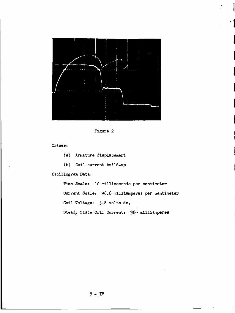
Figure 2

Tr&ces!

(a) Armature displacement

(b) Coil current build.up

Oscillogram Data:

Time Scale: lO milliseconds per centimeter

Current Scale: 96.6 milliamperes per centimeter


Steady State Coil Currentz 3_ milliamperes

8- IV

Figure 3

Traces.

(a)

(b)

Armature displacement

Coil current build-up

Oscillogr_mData:

Time Scale: I0 milliseconds per centimeter

Current Scale: 190 MiS_iamperes per centimenter



9-1V

Figure 4

Traces:

(a)

(b)

Armature displacement

Coil current build-up

Oscillogram Data:

Time Scale: l0 milliseconds per centimeter

Current Scale: _90 milliamperes per centimeter

Coil Voltage: 26 volts dc.


10- IV

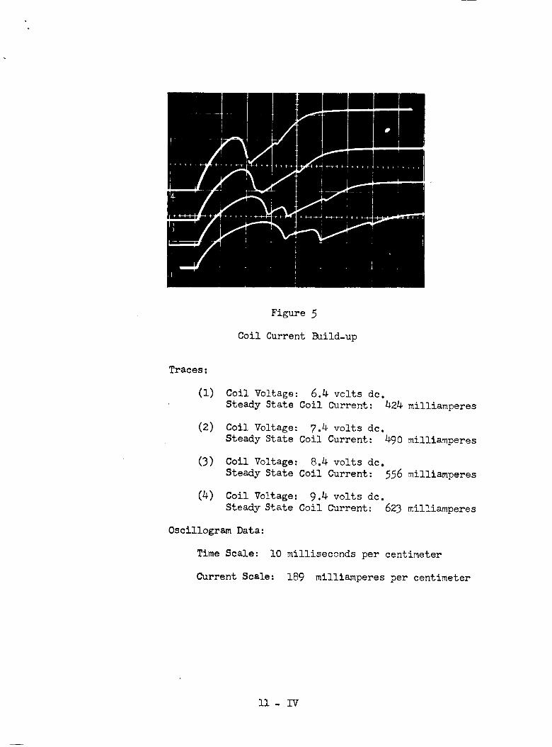
Figure 5


Traces:

(I) Coil Voltage: 6.4 volts dc.Steady State Coil Current: 424 milliamperes

(2) Coil Voltage: 7._ volts dc.Steady State Coil Current: 490 milliamperes

(3) Coil Voltage: 8.4 volts dc.Steady State Coil Current: 556 milliamperes

(4) Coil Voltage: 9.4 volts dc.Steady State Coil Current: 623 milliamperes

Oscillogram Data:

Time Scale: i0 milliseconds per centimeter

Current Scale: 189 milliamperes per centimeter

ll- IV

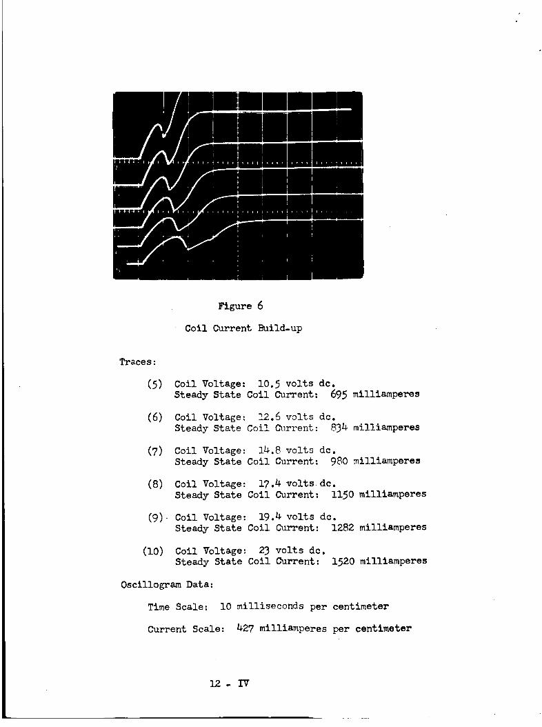
Figure 6


Traces:

(5) Coil Voltage: 10.5 volts dc.



Steady State Coil _Irrent: 834 milliamperes

(7) Coll Voltage: 14.8 volts dc.



Steady State Coil Current: llSO milliamperes



(lO) Coll Voltage: 23 volts dc.

Steady State Coll Current: 1520 milliamperes

OscillogramData:

Time Scale: lO milliseconds per centimeter

Current Scale: _27 milliamperes per centimeter

12° IV

TABLE OF CONTENTS

Part B

Vibration

Title

Interim

Section Report

Vibration Test .................. IV 2nd

Vibration Test Continued ............... II 3rd

Rose

Blue

Yellow

Ta_bb9olor Code

Ist Interim

2nd Interim

3rd Interim

1 January - 28 February, 1962

1 March - 30 April, 1962

I May - 30 June, 1962

SECTION IV

VIBPATION TEST

I

I

I

Failure of a relay under severe vibration is a common problem. This

investigation is being conducted with the following two goals in mind. First,

a particular group of relays shall be tested and an attempt made to determine

and correct the cause of failure for each individual relay. Second, it is

hoped that the study of these relays will produce some design criteria

(concerning vibration problems) for the class of relays in general.

The group of relays tested consisted of the following types:

(a) 25 amp, three sets of NO main contacts, one set NO and one set NC

auxiliary contacts

(b) 50 amp, one set of NO main contacts, one set NO and one set NC

auxiliary contacts

(c) 100 amp, one set of NO main contacts, one set NO and one set NC

auxiliary contacts

(d) 200 amp, one set of NO main contacts, one set NO and one set NC

auxiliary contacts.

Each type of relay was attached to the vibration table and checked for con-

tact failure over the frequency range of l0 to 2000 cps. (The relays were

energized at the rated coil voltage.) The following failures were noted:

(a) 25 amp relay - At a frequency of 390 cps, the center set of main

contacts failed at 14 g, the outer sets failed at 40 g. No fail-

ure of the auxiliary contacts was noted at this frequency.

(b) 50 amp relay- At 1300 cps, the main contacts failed at I0 g. No

failure of the auxiliary contacts was noted at this frequency.

(c) lO0 amp relay - At 680 cps, the main contacts failed at 17.7 g.

No failure of the auxiliary contacts was noted at this frequency.

1 - IV

(d) 200 amp relay . At 960 cps, the main contacts failed at 14 g. No

failure of the auxiliary contacts was noted at this frequency.

It should be noted that relays of the same type were found to correspond

as to the frequency at which failure occurred and varied only slightly in

the level of acceleration required.

In view of the results of the first test it was decided to check on the

possibility of armature motion while energized and its relation, if any, to

the failures.

The 100 amp relay was chosen for the studyof armature motion. Photo-

graphs were taken of the coil current and the contact voltage to obtain a

permanent record of results.

Figure 1 shows the coil current and contact voltage of the 100 amp relay

undergoing 17.7 g's at 680 cps. The upper trace is the contact voltage, the

lower trace is the coil current. The coil voltage is lO volts. The two

traces indicate that opening of the contacts corresponds to the motion of

the armature. Note that the contacts stay open longer every other time and

this corresponds to a more extreme armature displacement.

Figure 2 shows the same relay under the same conditions, except that

the coil voltage is increased to 28 volts. The coil current indicates less

armature motion, but the contacts continue to open.

In Figure 3, the coil voltage has been raised to 50 volts. This has

noticeably reduced the armature motion but seems to have little effect on

the contact failure.

Another possible cause of contact failure is the flexing of the

stationary contact mounts which pass through the case of the relay. In order

to investigate this possibility, the mounting studs for the contacts were

braced to the upper part of the relay case. The results are shown in

Figures 4, 5 and 6.

2- IV

In Figure _, with I0 volts applied to the coil, the contacts are seen

to open at a higher frequency (760 cps.) The armature motion is noticeably

less than in Figure I, which :ms without the braced mountings. The contacts

no longer fail at 680 cps. as they did _ithout the brace.

The same pattern of failure occurs in Figures 5 and 6 with the armature

motion becoming less as the coll voltage is increased.

The result of bracing the contacts then seems to be a reduction of

armature motion and a change in the frequency at which failure occurred.

A second I00 amp relay was tested with the contacts braced, with the

result shown in Figure 7. With 28 volts applied to the coil, there seems

to be very little armature motion, although the contacts are opening.

Figure 8 shows the same relay _lth the brace removed and I0 volts

applied to 'the coil. The coil current indicates a much greater motion of

the armature. The failure frequency has returned to the 680 cps. as was

the case in Figure I.

The result of increasing the coil voltage to 50 volts is shown in

Figure 9. The armature motion is reduced with no apparent affect on the

contacts.

A 25 amp relay was tested with a blocked armature. The effect of block-

ing the armature was only to change the frequency at which the contacts opened.

This seems to indicate that the problem is not the armature but with the

contacts themselves. A series of test to investigate the contacts and their

mountings is now underway. Only one permanent failure was noted in these

tests. This took place on the _0 ampere relay during the vibration test.

The NC auxiliary contacts broke loose from the mounting which was detected

after the vibration test was completed.

From information of tests conducted at NASA, 3 out of I0 relays tested

failed in the same manner. This seems to indicate that the auxiliary

3-IV

contacts need morebracing.

The results of the test performed to date are inconclusive, but it is

hoped that _ith the results of additional tests, a clear picture of the

cause of contact failure on these relays can be established.

4 - IV

Figure 1

T_aces:

Top trace:

Lo_er trace:

Oscillogram Data:

Relay . IO0 amp #I

Contacts - NO (main)

Coil Voltage . lO_volts

Time Scale . .5 ms per cm

Current Scale - i ma per cm


Frequency . 680 cps

Acceleration - 17.7 g (rms)

Contact Voltage

Coil Current

5- IV

Figure 2

Traces:

Top Trace:

Lower Trace:

Oscillogram Data:

Relay - I00 amp _I



Time Scale - .5 ms per cm



Frequency - 680 cps


Contact Voltage

Coil Current

6- IV

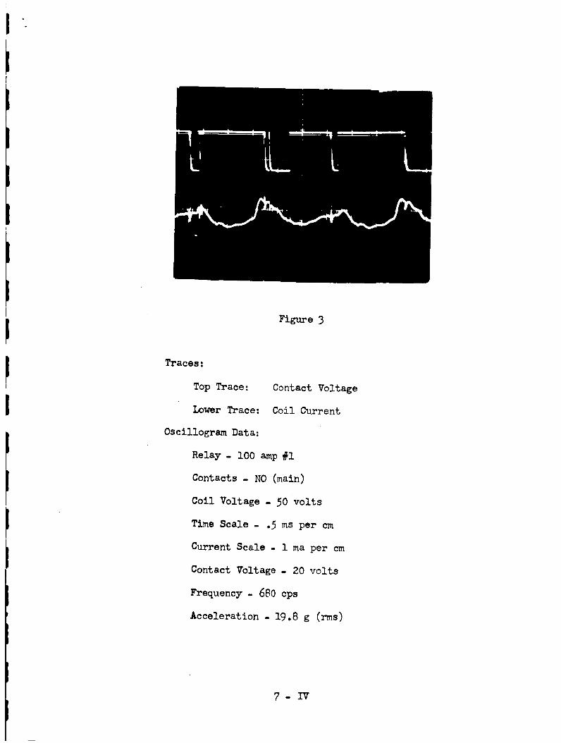
Figure 3

Traces:

Top Trace:

Lower Trace:

OscillogramData:

Contact Voltage

Coil Current

Relay - I00 amp #I






Frequency - 680 cps


7- IV

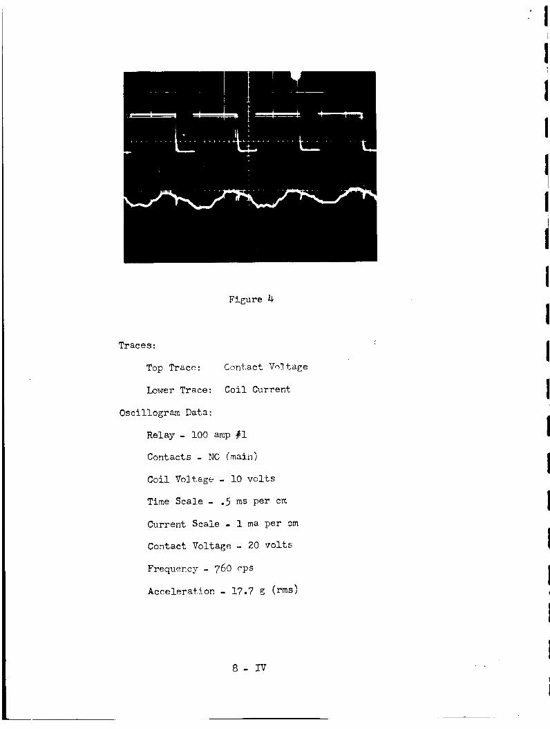
Figure 4

Traces:

Top Trace:

Lower Trace:

Osci!!ogram Data:

Contact Voltage

Coil Current

Relay - i00 amp#I

Contacts - NO(main)

Coil Voltage - !0 volts




Frequency - 760 cps


8- IV

I

I+

I

I

I

I

I

l

I

I

I

I

I

l

Figure 5

Traces:

Top Trace:

Lower Trace:

OscillogramData:

Contact Voltage

Coil Current

Relay - 100 map #I






Frequency - 760 cps

Acceleration - 17,7 g (rms)

9- IV

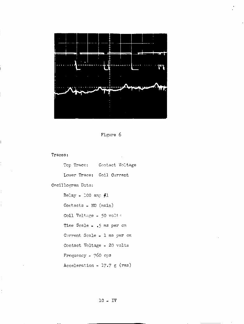
Figure 6

Traces :

Top Trace :

Lower Trace :

Oscillogram Data:

Relay - 100 amp #l


Coil Voltage - 50 vol_


C_rrent Scale - 1 ma per cm


Frequency- 760 cps

Acceleration- 17.7 g (rms)

Contact Voltage

Coil Current

lO- IV

l

T

I

Figure 7

Traces:

Top Trace:

Lower Trace:

Oscillogram Data:

Contact Voltage

Coil Current

Relay - I00 amp #2


Coil Voltage - 28volts


Current Scale - I ma per cm

ContaCt Voltage - 20 volts

Frequency - 750 cps


ll. IV

Figure 8

Traces:

Top Trace:

Lower Trace:

Oscillogram Data:

Contact Voltage

Coil Current

Relay . I00 amp 92


Coil Voltage - I0 volts




Frequency - 680 cps


12- IV

Figure 9

Traces:

Top Trace:

Lower Trace:

OscillogramData:

Contact Voltage

Coil Current

Relay. 100 amp #2






Frequency - 680 cps

Acceleration . 14.1 g (rms)

13 - IV

VIR_ATION TESTING

In order to have a more logical procedure to follow in the search

for the cause of separation of contacts when the relays under consid-

eration are subjected to extreme vibration, the contact system was

examined to determine all the possible causes of separation. The system

under consideration is shown in Figure i.

Ft_e I. Relay Contact System

The possible causes of separation of the contacts are listed below:

I- II

I) Motion of point 1 with respect to point 2

2) Motion of point 5 with respect to point 2




Consider cause number one. Any movement of point 1 with respect

to 2 would be a result of flexing the case enclosing the relay. This

is definitely a possibility on the relays tested. If experimental

evidence does show the case to be flexing to a harmful degree, a re-

location of the mounting bracket to the center of the case would be

a possible solution to the problem.

If the armature were to move with respect to the coil (cause

number two), the contacts could easily open. This possibility has pre-

viously been investigated on several relays and the evidence obtained

to date seems to Justify the elimination of this cause from consideration

for the present.

The movable contacts are mounted on a bar which is allowed to move

on the armature shaft in order to provide some armature overtravel. This

bar is restrained by two springs. It seems very likely that this arrange-

ment could produce a separation of the contacts at the resonant frequency

of the spring and mass system. This cause will be discussed at greater

length later in the report.

The stationary contacts, being mounted as long cantilevers, are

very susceptible to vibrations. Any extreme motion caused by flexing of

the mounting or in the bar itself could possibly open the contacts.

This cause is also considered worthy of some investigation.

A flexing of the movable contact bar itself is considered unlikely

because of the rigidity of this particular part.

2- II

i

i

II

I

I

I

I

I

I

I

I

The list of possible causes has now been reduced to three. Of these

three, the most likely cause is believed to be number three_ therefore,

this was the next topic to be investigated. It should be poihted out

that the failure is not necessarily due to one condition alone but could

be a result of several conditions.

Investigation of overtravel spring system

It was felt that the one characteristic that would have the greatest

effect on the contact failure was the motion of the movable contact

bar with respect to the armature shaft. In order to check on this

possibility, two relays were opened by sawing a small round hole in the

base such that the adjusting nut on the end of the armature shaft could

be reached. Both relays were then checked for failure at several spring

tension adjustments. The results are as follows:

I00 amp relay #I

With the original manufactures adjustment of the spring system the

main contacts failed at a frequency of 830 cycles per second. The re-

quired R.M.S. acceleration level was 15.5G. This was the only frequency

at which any failure was noted. Figure 2 shows the opening of the

contacts (top trace) and the exciting current of the vibration table

(lower trace). The picture was Steady on the oscilloscope as it appears

in the figure.

The spring was loosened approximately four turns of the adjusting

nut. The results are shown in figures 3 and 4. The failure is con-

tinuous over the entire frequency range of 20 to 2000 cps. Very low

values (3 to 9 G) of acceleration were required.

Increasing the spring tension by about one turn yielded the failure

shown in figure 5. Note that 21G is required to open the contacts and

the frequency has shifted about eighty cycles. The change in frequency

3- II

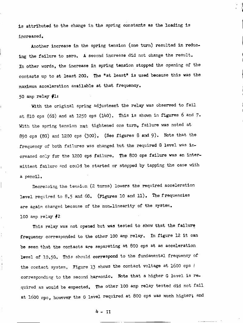
is attributed to the change in the spring constants as the loading is

increased.

Another increase in the spring tension (one turn) resulted in reduc-

ing the failure to zero. A second increase did not change the result.

In other words, the increase in spring tension stopped the opening of the

contacts up to at least 20G. The "at least" is used because this was the

maximumacceleration available at that frequency.

50 amprelay#l:

With the original spring adjustment the relay was observed to fail

at 810 cps (6G) and at 1250 cps (14G). This is shownin figures 6 and 7.

With the spring tension nut tightened one turn, failure was noted at

890 cps (SG) and 1200 cps (30G). (See figures 8 and 9). Note that the

frequency of both failures was changed but the required G level was in-

creased only for the 1200 cps failure. The 800 cps failure was an inter-

mittent failure and could be started or stopped by tapping the case with

a pencil.

Decreasing the tension (2 turns) lowers the required acceleration

level required to 8.5 and 6G. (Figures I0 and ll). Thefrequencies

are again changed because of the non-linearity of the system.

lO0 amprelay _2

This relay was not opened but was tested to show that the failure

frequency corresponded to the other lO0 amprelay. In figure 12 it can

be seen that the contacts are separating at 800 cps at an acceleration

level of 10.SG. This should correspond to the fundamental frequency of

the contact system. Figure 13 shows the contact voltage at 1600 cps !

corresponding to the second harmonic. Note that a higher G level is re.

quired as would be expected. The other 100 amprelay tested did not fail

at 1600 cp_, however the G level required at 800 cps was muchhigher; and

_- II

it is assumed that the equipment was not capable of producing the accelera-

tion required at 1600 cps to separate the contacts.

The results of these tests seem to indicate that the present problem

of failure is the result of an improper adjustment of the overtravel and

back tension springs. The next planned study will be to verify more com-

pletely the results of this test, and then to proceed with the formula-

tion of the necessary relationships in order that the design of this system

of contacts can be incorporated into the already existing relay design

procedure •

5- II

Figure 2

Traces :

Upper Trace:

Lower Trace:

Oscillogram Data:

Relay - lO0 amp #1

Contacts - NO (Main)



Contact Voltage - lO volts

Frequency - 830 cps

Acceleration - 15.5 G (rms)

Contact Voltage

Exciter Current

6- II

Figure 3

_z'aces:

Upper Trace:

Lower Trace:

OscillogramData:

Contact Voltage

Exciter Current

Relay - I00 amp #I





Frequency - 795 cps


7- II

Figure 4

Opper Trace: Contact Voltage

Lower Trace: Exciter Current

O;_d llogram Data:

Re]ay- lO0 amp #l

Contacts- NO (Main)

Cc_l Voltage - 28 volts

T_me Scale - 1 ms per cm

Co_ act Voltage - lO volts

Frequoncy - 385 cps

Ac_lo_tion- _.5 G (rms)

8- II

Traces_

Upper Trace:

Lower Trace:

OscillogramData:

Figure 5

Contact Voltage

Exciter Current

Relay- I00 amp #I


Coil Voltage - 28-volts

Time Scale . I ms per cm

Contact Voltage - I0 volts

Frequency- 750 cps

Acceleration - 21 G (rms)

9- II

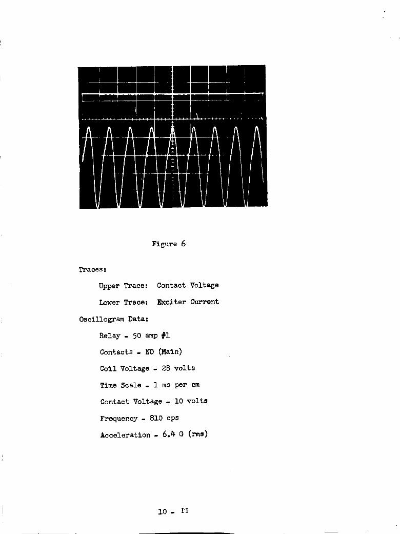
Figure 6

Traces:

Upper Trace:

Lower Trace:

Oscillogram Data:

Relay- 50 amp#l

Contacts - NO(Main)

Coll Voltage - 28 volts



Frequency - 810 cps

Acceleration - 6._ G (rms)

Contact Voltage

Exciter Current

I0- I I

Figure 7

Traces:

Upper Trace-

Lower Trace:

Oscillogram Data:

Relay- 50 amp _I



Time Scale - I ms per cm


Frequency. 1250 cps

Acceleration- 14 G (rms)

Contact Voltage

Exciter Current

II - II

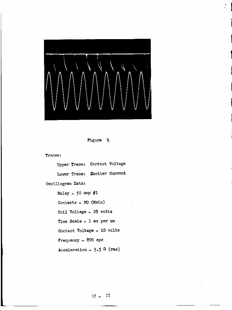
Figure

Traces:

Upper Trace:

Lower Trace:

Oscillogram Data:

Contact Voltage

Exciter Current

Relay- 50 amp #I





Frequency - 890 cps


[2 . II

Figure 9

Traces z

Upper Tracez

Lower Trace:

Oscillogram Data:

Relay - 50 amp #I


Coil Voltage- 28 volts



Frequency- 1200 cps


Contact Voltage

Exciter Current

13" II

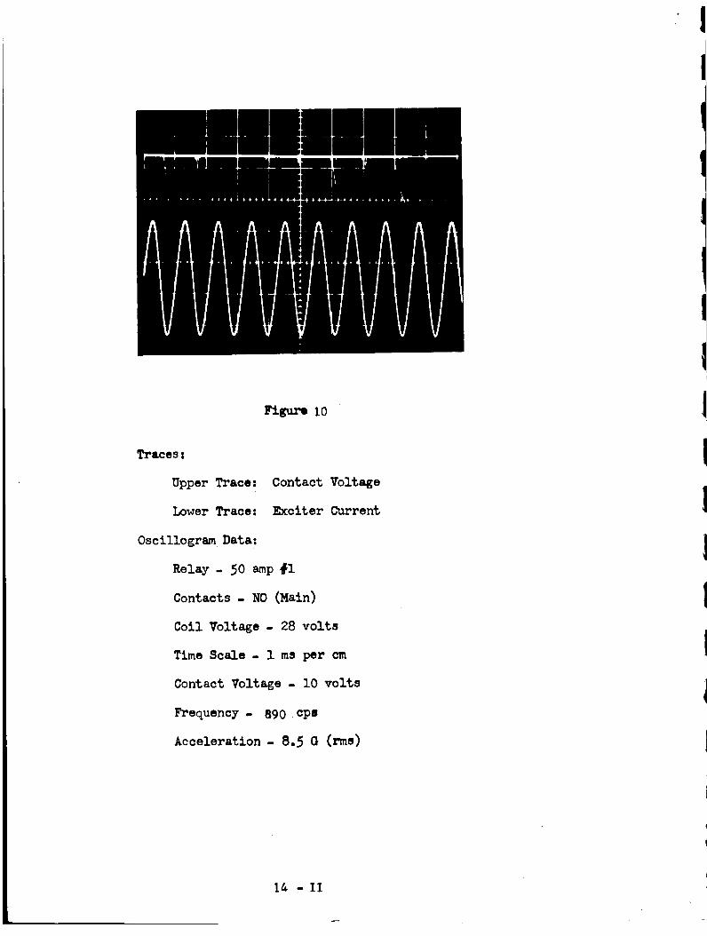
Figure I0

Traces

Upper Trace:

Lower Trace:

Oscillogram Data:

Relay- 50 amp #I




Contact Voltage - i0 volts

Frequency - 890 cps

Acceleration- 8.5 G (rms)

Contact Voltage

Exciter Current

l& - II

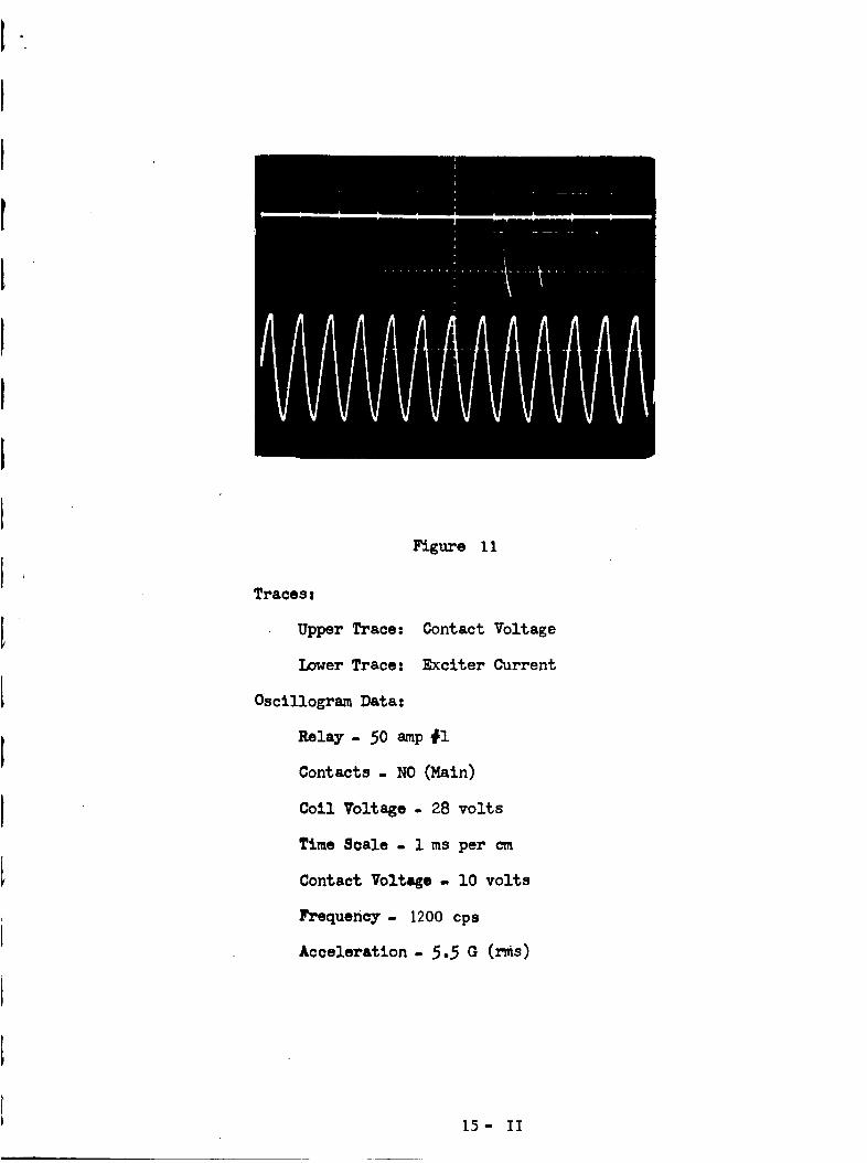
Tracesl

Upper Trace:

Lower Trace:

OscillogramData:

Figure 11

Contact Voltage

Exciter Current

Relay - 50 amp #I





Frequency- 1200 cps

Acceleration- 5.5 G (rms)

15- II

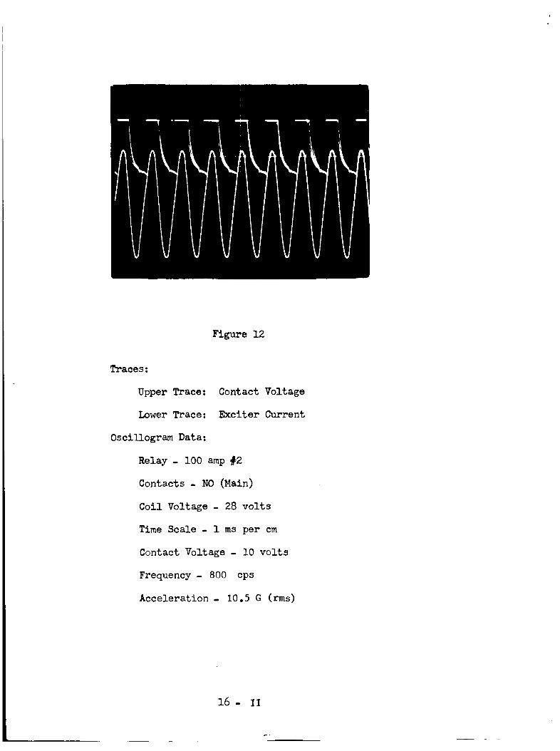
Figure 12

Traces:

Upper Trace: Contact Voltage

Lower Trace: Exciter Current

Oscillogram Data:

Relay - 100 amp#2




Contact Voltage - l0 volts

Frequency - 800 cps


16- II

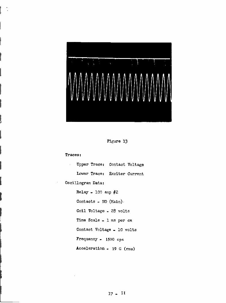
Figure 13

Traces:

Upper Trace:

Lower Trace:

Oscillogram Data:

Relay- I00 amp #2

Contacts - NO (Main),


Time Scale- 1 ms per cm

Contact Voltage - l0 volts

Frequency- 1600 cps


Contact Voltage

Exciter Current

17 - I-I

TABLE OF CONTENTS

Part C

Contact Study

Title

Interim

Section Report

Preliminary Investigation and Proposal

of Relay Contact Design ............... III ist

Contact Rating ................. II 2nd

Theoretical Investigation and Some Experimental

Data for an Electrical Contact Failure CaUsed by

Electrical Loading .............. III 2nd

Further Discussion of Contact Failure Due

to Electrical Loading ............ - - III 3rd

Rose

Blue

Yellow

Tab Color Code

ist Interim

2nd Interim

3rd Interim


i March - 30 April, 1962

i May - 30 June, 1962

SECTIONIII

PRELDIINARYI_VESTIGATIONA_DPROFOSALOFRELAYCONTACTDESIGN

This section is concerned with someproblems dealing with the design

of a relay contact system, given the specifications. In particular, the

t3_e of contact systems of immediate interest are of the heavy duty

(current) t_e. However, in order to arrive at a design procedure for

these types, a more general discussion is needed at this time due to the

lack of information concerning contact design.

The first portion of this section, Part I, is a discussion of some

design terminology which is frequently used but seldom defined. Some

definitions are given _ith the intent of adding clarity to discussions in

subsequent reports. Also, someproblems related to these definitions are

discussed.

The second phase of this section, Part II, deals _,ith the particular

t}_e of relay, to be evaluated and re-designed under the present research

contract. The discussion is limited to the contact system and the speci-

fications which will govern their design. The requirements for the mechan-

ical design and electrical design are separated, and the preliminary

investigation of these factors is given. Someoscillograms of particular

electrical loads are given at the end of this section in connection with

this initial evaluation report.

The final topic to be presented, Part III, is a proposal directed at

the problem of designing contacts to satisfy the electrical load require-

ments. _vo basic assumptions are presented with the intent of obtaining

a single parameter with which to relate duty cycle, type current load,

relay discharge time and obtain the probable number of operations to fail-

ure due to electrical properties.

1 -III

PARTI

The contact design problem is difficult for manyreasons. One of these

reasons is because of the lack of methods and communication for the design

process itself. The following discussion is intended to give more concrete

definition to someof the basic concepts used in design. The following

ideas are defined in terms of the quantities, system, criteria, parameter,

relationship and restricted. DesiF_n: The construction of a system based

on criteria _ll be called design. (This will be denoted by the design of

(S) when referring to a particular system.)

Set of Specifications: A collection of criteria (denoted by [ci].

and a collection of parameters (denoted by [Pj]) is said to form a set of

specifications (denoted by [Sr] ) if:

(i) For each criteria [ci] there is a relationship (denoted by fi)

such that, fi([Pj]) restricts a subset [Pj]. (If this restric-

ted set is denoted by [Sp] i then fi([Pj])----_[SP]i can be used

to denote (i), v_ere-----_stands for implies.) The set [St] is

the totality of the restricted parameters.

The above definition emphasizes the complexity involved, of taking

a requirement for design and obtaining a set of specifications. The

undefined quantities: parameter and restricted, are usually well under-

stood for any particular case. For example, physical quantities, (volt-

age (E), time (t), temperature (T), etc.), are very commonly used as

parameters. Restricted, for many cases is defined as; assigning a value

or range of values to a parameter. The more difficult problem is that of

selecting the set of parameters, and the relationships, from the given

criteria, which in turn restrict the parameters. Many examples could be

given in which this can be easily done, but for the most part this is a

2- III

difficult problem due to the nature of the set o_ criteria. Part II is an

illustration of the problems involved in this type criteria.

Design Process: A process which uses a fixed set of criteria and

yields a design for (S) will be called, a design process.

A best design is any system (S) which has the followingBest Desk:

properties.

(i)

(ii)

The design of (s) was a design process

The criteria for the design process formsa set of specifications

(iii) The system has a set of parameters, a

subset of these being the same as the set

of specifications in (ii).

This definition is nothing more than a formal statement of the common

conception usually associated with this idea. That is, a best design

produces a system which has all the properties whic_ initiated the design.

Note, however, that this definition disallows variable criteria when discus-

sing the best design, and parameters belonging to the system _ich do not

belong to the set formed by the fixed criteria. Also, note that a best

design is not necessarily unique. Although a best design in each design

problem would be the ultimate, this does not appear to be the actual

situation. For this reason the following definition appears to be more

useful when evaluating designs which have no evaluating criteria given.

Bette_____rDesign:Let two designs, say d: and dz, be such that the same

criteria is used in the design of dl and dz, and for any set of specifica-

tions [Sr] formed by the criteria for dl and dz are not both best designs.

Then dl is said to be a better design and d2 if the parameters of d2

(denoted by [P=]) and dl (denoted by [P:]) have the following property.

[Pz]_[Sr]_[P_]_[Sr] where A_B denotes, parameters common between A

and B, and ACB denotes that B has all the parameters of A plus some more.

3- III

This definition allows two designs to be compared assuming that not

both are best designs. The comparison is a matter of seeing which design

comes closest to a best design relative to a common basis. The common basis

is most important since without this property the comparison of two designs

becomes arbitrary when no comparison criteria is included in the criteria

for design.

Before leaving Part I it is mentioned again that the preceeding discus-

sion is only intended to point out some of the main problems concerned with

initiating and terminating a design. The discussion of best and better

designs indicates reasons for the many different opinions relating to a

good design. Although these opinions many times have a good motivation

seldom can they be used by the designer until a system has been designed.

Even though the definitions were given in a general form it is felt that

to have a basis for ideas involved in a problem is very useful. Also,

since converting from a general case to a particular case is much easier

than the converse problem it is hoped that the satisfactory solution to

the problem at hand will be enhanced by the above structure.

PART II

As mentioned in Part I it is usually a difficult task to take a set

of criteria and form a set of specifications. Also, except for a few

cases a design process which has well defined steps for producing a system

is available. Although the objective of this study is to obtain a better

design for a particular system the above problems enter into the realiza-

tion of this objective. This is the case since no design process is

available with which to handle the given criteria, and the set of specifi-

cations formed by the given criteria has not been determined.

4- III

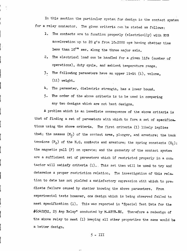
In this section the particular system for design is the contact system

for a relay contactor. The given criteria can be stated as follows:

1. The contacts are to function properly (electrically) with RNS

acceleration up to 20 g's from 10-2000 cps having chatter time

less than lO"_ sec. along the three major axis.

2. The electrical load can be handled for a given life (number of

operations), duty cycle, and ambient temperature range.

3. The following parameters have an upper limit (i), volume,

(il) weight.

4. The parameter, dielectric strength, has a lower bound.

5. The order of the above criteria is to be used in comparing

any two designs which are not best designs.

A problem which is an immediate consequence of the above criteria is

that of finding a set of parameters with which to form a set of specifica-

tions using the above criteria. The first criteria (1) likely implies

that; the masses (Mj) of the contact arms, plunger, and armature; the back

tensions (Po) of the N.C. contacts and armature; the spring constants (Ki) ;

the magnetic pull (F) on operate; and the geometry of the contact system

are a sufficient set of parameters which if restricted properly in a con-

tactor will satisfy criteria (1). This set then will be used to try and

determine a proper restriction relation. The investigation of this rela-

tion to date has not yielded a satisfactory expression with which to pre-

dicate failure caused by chatter knowing the above parameters. From

experimental tests however, one design which is being observed failed to

meet specification (1). This was reported in "Special Test Data for the

#6042H32, 25 Amp Relay" conducted by M-AST_-EC. Therefore a redesign of

the above relay to meet (1) keeping all other properties the same would be

a better design.

5 -III

Specification (2) is not as easily broken into a set of identifiable

parameters as was (1). Also a procedure for relating the parameters in-

volved in this set of specifications into someusable relationships has

not been developed at the present time. In this particular design investi-

gation the problem is compoundedby the variable nature of the electrical

load and duty cycle. The electrical load has been tentatively divided

into the following specifications.

(a) Maximuminrush current%twlce rated current with a specified

time interval.

(b) For inductive load the time constant must be specified along

with rated current.

(c) The type of circuit voltage (AC, DC) and desired value should

be specified for all loads.

(d) For resistive load the rated current should be specified.

Although no definite relationships have been found with which to

handle the specifications of (2) in an analytical manner the following

investigations have been initiated.

A. In order to handle the stady state (or rated) value of contact

current, assumean ambient and maximumtemperature distribution

for the contact structure, and develop a set of relationships

which can predict this distribution. The following parameters

are desirable to belong to these relationships.

(1)

(2)

(3)

(4)

Ic = current through contacts

VcRc = I_ = loaded contact resistance

Contact dimensions

Ambient temperature and maximum allowable temperature

distribution

(5) Contact material (mass desity, specific heat)

6- III

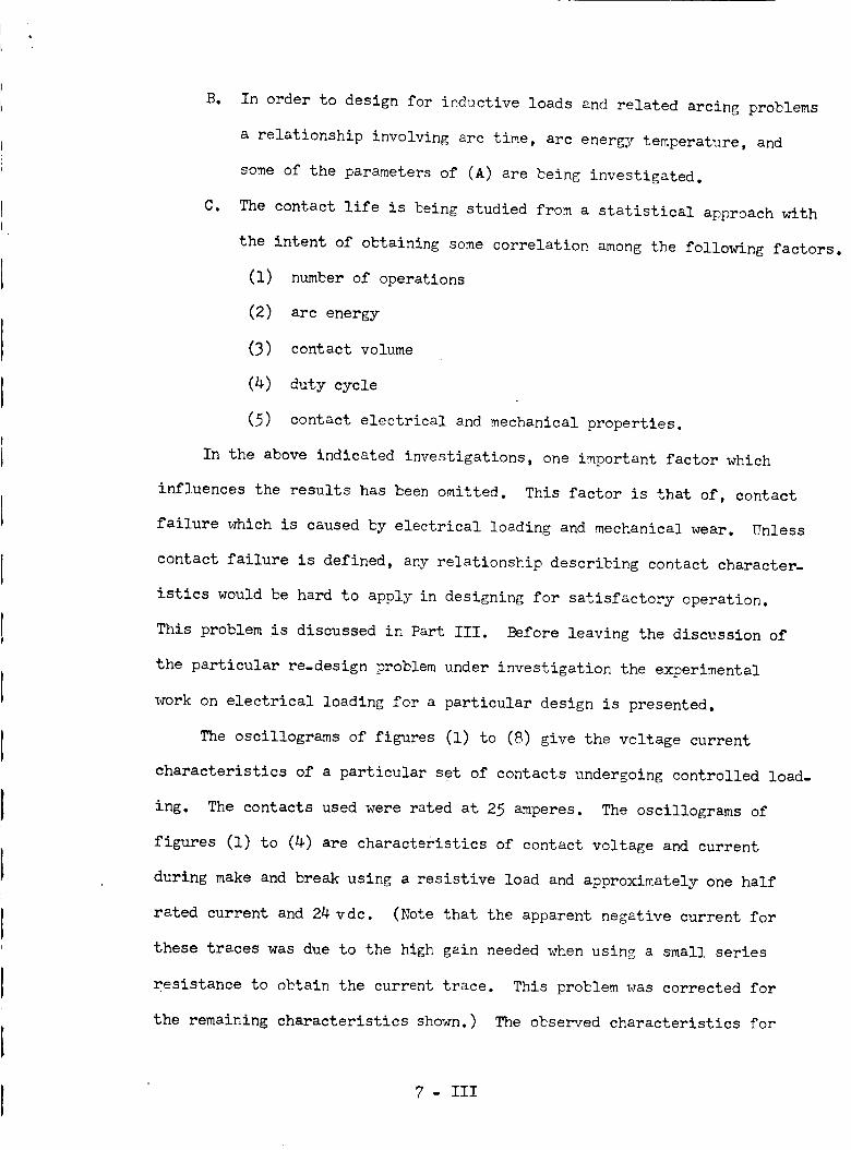
B. In order to design for inductive loads and related arcing problems

a relationship involving arc time, arc energy temperature, and

some of the parameters of (A) are being investigated.

C. The contact life is being studied from a statistical approach with

the intent of obtaining some correlation among the following factors.

(1) number of operations

(2) arc energy

(3) contact volume

(4) duty cycle

(5) contact electrical and mechanical properties.

In the above indicated investigations, one important factor which

influences the results has been omitted. This factor is that of, contact

failure which is caused by electrical loading and mechanical wear. Unless

contact failure is defined, any relationship describing contact character-

istics would be hard to apply in designing for satisfactory operation.

This problem is discussed in Part III. Before leaving the discussion of

the particular re-design problem under investigation the experimental

work on electrical loading for a particular design is presented.

The oscillograms of figures (1) to (8) give the voltage current

characteristics of a particular set of contacts undergoing controlled load-

ing. The contacts used were rated at 25 amperes. The oscillograms of

figures (1) to (4) are characteristics of contact voltage and current

during make and break using a resistive load and approximately one half

rated current and 24 vdc. (Note that the apparent negative current for

these traces was due to the high gain needed when using a small series

resistance to obtain the current trace. This problem was corrected for

the remaining characteristics shown.) The observed characteristics for

7- III

these contacts under resistive load using the duty cycle ll sec. on -

sec. off, after 4000 operations as compared to the original character-

istics, was essentially unchanged, if not improved from the standpoint of

arcing on release. The temperature increase of the contact terminals over

that produced by the coil was not measurable at room temperature. The

contact resistance under load also had no apparent change. After this

period of testing the load was changed to an inductive load keeping the

duty cycle as before. Oscillogram (5) gives the contact voltage and

current on release when the relay was cold (ten operations) at approximate-

ly one half rated current and 24 v dc. The blow-out of the arc is clearly

marked by the impulse of voltage which accompanies this process in induc-

tive circuits. Note, however, that the current does not extinguish until

the current decays to near zero. This causes the arc time to be of the

order 200-300 times greater than for the resistive case. The arc energy

calculated as

AE = --QT°VcIc dtoj

can be compared for these two cycles and different type loads using the

information given in oscillogr_ms (3) and (5). This was done using

Vc = 12 volts, Ic = _ amps, TO = (.06)(.25)ms for the resistive case. For

the inductive case increments of 2 ms were used and the integral computed

numerically using mean current and voltage during each interval.

AE for resistive load = (7.2)10 "3 watt-sec.

AE for inductive load = (1451)10 "s watt-sec.

Due to the large differences in the above arc energies the relay was cycled

250 and 750 operations using the duty cycle mentioned earlier. Oscillo-

gram (7) and (8) give the characteristics at the end of the above periods

respectively. The operate characteristics are also given in these last

8- III

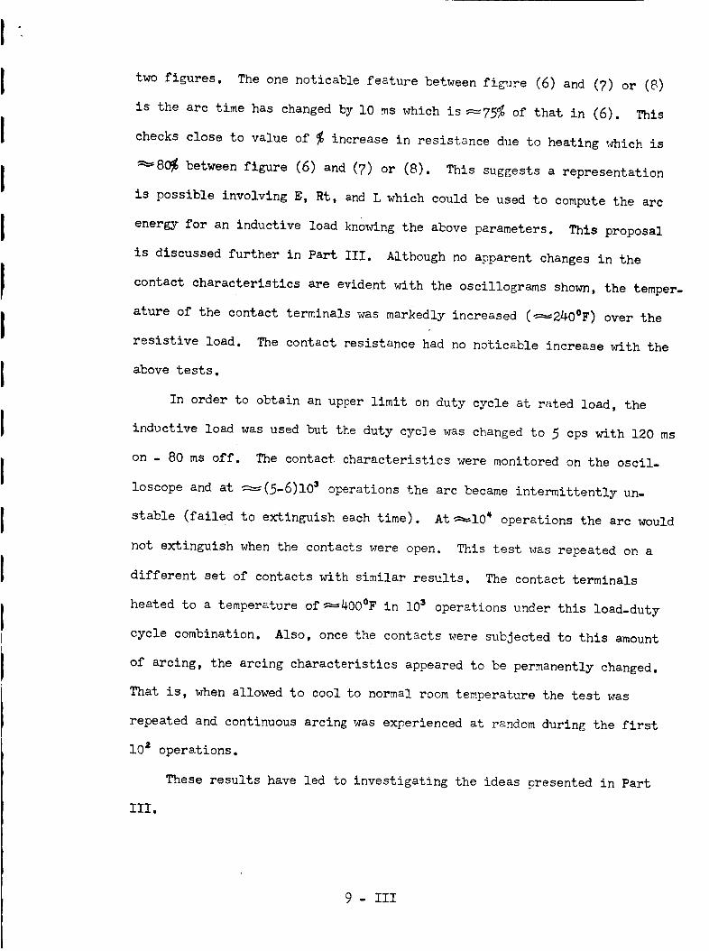
I

two figures. The one noticable feature between figure (6) and (7) or (8)

is the arc time has changed by I0 ms which is_75% of that in (6). This

checks close to value of % increase in resistance due to heating which is

_80% between figure (6) and (7) or (8). This suggests a representation

is possible involving E, Rt, and L which could be used to compute the arc

energy for an inductive load knowing the above parameters. This proposal

is discussed further in Part III. Although no apparent changes in the

contact characteristics are evident with the oscillograms shown, the temper-

ature of the contact terminals was markedly increased (_2_OeF) over the

resistive load. The contact resistance had no noticable increase with the

above tests.

In order to obtain an upper limit on duty cycle at rated load, the

inductive load was used but the duty cycle was changed to 5 cps with 120 ms

on - 80 ms off. The contact characteristics were monitored on the oscil-

loscope and at _(5-6)103 operations the arc became intermittently un-

stable (failed to extinguish each time). At_10 _ operations the arc would

not extinguish when the contacts were open. This test was repeated on a

different set of contacts with similar results. The contact terminals

heated to a temperature of_00eF in 103 operations under this load-duty

cycle combination. Also, once the contacts were subjected to this amount

of arcing, the arcing characteristics appeared to be permanently changed.

That is, when allowed to cool to normal room temperature the test was

repeated and continuous arcing was experienced at random during the first

l02 operations.

These results have led to investigating the ideas presented in Part

III.

9- III

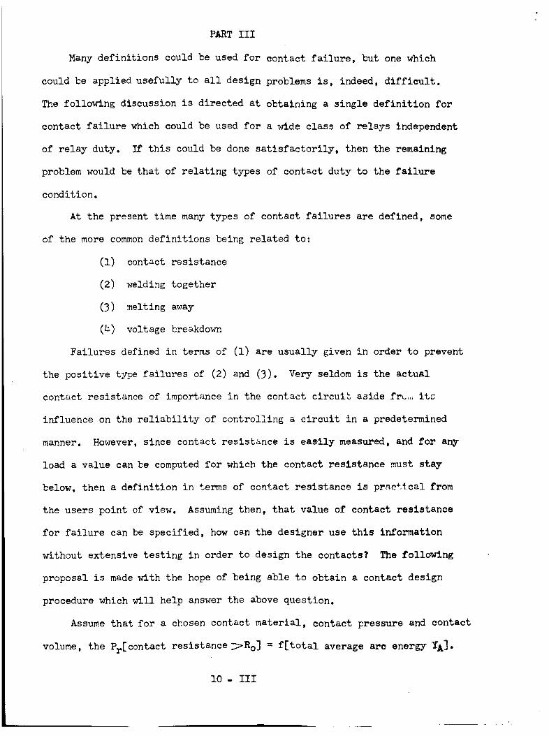
PARTIII

Manydefinitions could be used for contact failure, but one which

could be applied usefully to all design problems is, indeed, difficult.

The following discussion is directed at obtaining a single definition for

contact failure which could be used for a wide class of relays independent

of relay duty. If this could be done satisfactorily, then the remaining

problem would be that of relating types of contact duty to the failure

condition.

At the present time manytypes of contact failures are defined, some

of the more commondefinitions being related to:

(1) contact resistance

(2) welding together

(3) melting away

(4) voltage breakdown

Failures defined in terms of (1) are usually given in order to prevent

the positive type failures of (2) and (3). Very seldom is the actual

contact resistance of importance in the contact circuit aside fr_, its

influence on the reliability of controlling a circuit in a predetermined

manner. However, since contact resistance is easily measured, and for any

load a value can be computedfor which the contact resistance must stay

below, then a definition in terms of contact resistance is prac£1cal from

the users point of view. Assuming then, that value of contact resistance

for failure can be specified, how can the designer use this information

without extensive testing in order to design the contacts? The following

proposal is madewith the hope of being able to obtain a contact design

procedure which will help answer the above question.

Assumethat for a chosen contact material, contact pressure and contact

volume, the Pr[contact resistance_Ro] = f[total average arc energY YA].

l0 -III

m

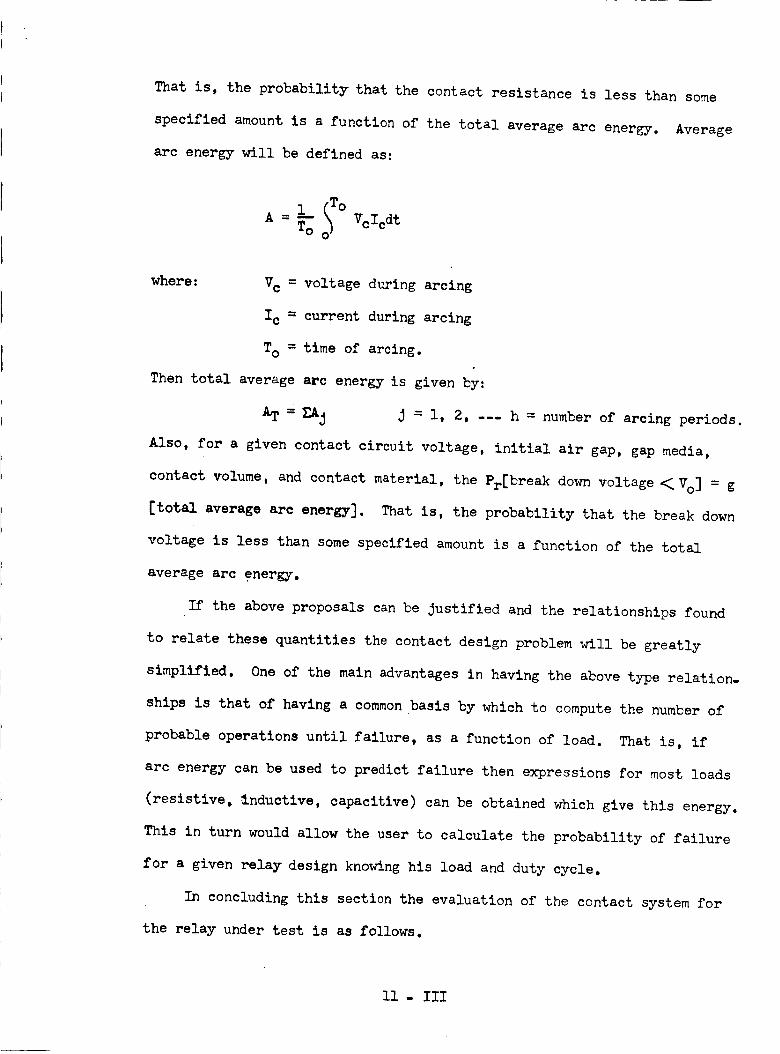
That is, the probability that the contact resistance is less than some

specified amount is a function of the total average arc energy. Average

arc energy will be defined as:

i_ T° VclcdtA = To

where: Vc = voltage during arcing

Ic = current during arcing

To = time of arcing.

Then total average arc energy is given by:

AT _Aj J = l, 2, --- h = number of arcing periods.

Also, for a given contact circuit voltage, initial air gap, gap media,

contact volume, and contact material, the Pr[break down voltage_Vo] = g

[total average arc energy]. That is, the probability that the break down

voltage is less than some specified amount is a function of the total

average arc energy.

If the above proposals can be Justified and the relationships found

to relate these quantities the contact design problem will be greatly

simplified. One of the main advantages in having the above type relation-

ships is that of having a common basis by which to compute the number of

probable operations until failure, as a function of load. That is, if

arc energy can be used to predict failure then expressions for most loads

(resistive, inductive, capacitive) can be obtained which give this energy.

This in turn would allow the user to calculate the probability of failure

for a given relay design knowing his load and duty cycle.

In concluding this section the evaluation of the contact system for

the relay under test is as follows.

II -III

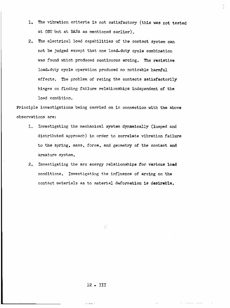
1. The vibration criteria is not satisfactory (this was not tested

at OSUbut at NASAas mentioned earlier).

2. The electrical load capabilities of the contact system can

not be judged except that one load-duty cycle combination

was found which produced continuous arcing. The resistive

load-duty cycle operation produced no noticable harmful

effects. The problem of rating the contacts satisfactorily

hinges on finding failure relationships independent of the

load condition.

Principle investigations being carried on in connection with the above

observations are:

1. Investigating the mechanical system dynamically (lumped and

distributed approach) in order to correlate vibration failure

to the spring, mass, force, and geometry of the contact and

armature system.

2. Investigating the arc energy relationships for Various load

conditions. Investigating the influence of arcing on the

contact materials as to material deformation is desirable.

12 -III

Oscillogram #l

Contact Voltage on Operate After 2000 OperationsUsing Resistive Load for 25 ampContactor

Traces:

(a) V_ltage

(b) Current

Duty Cycle - ll seconds on, 4 seconds off

0scillogram Data:

Time scale: .25 ms/cm

Voltage Scale: 20 v/cm

Current Scale: 50 mv/cm

Steady State Contact Current = 13 amps

Relay Operated ate28 volts

13 - iii

0scillogram#2

Contact Voltage and Current on Release After 2000

Operations Using Resistive Load for 25 amp Contactor

Traces:

(a) Voltage

(b) Current

Duty Cycle - ii seconds on, _ seconds off

0scillogram Data:

Time Scale: .25 m_/cm

Voltage Scale: 20 v/c_




14 - III

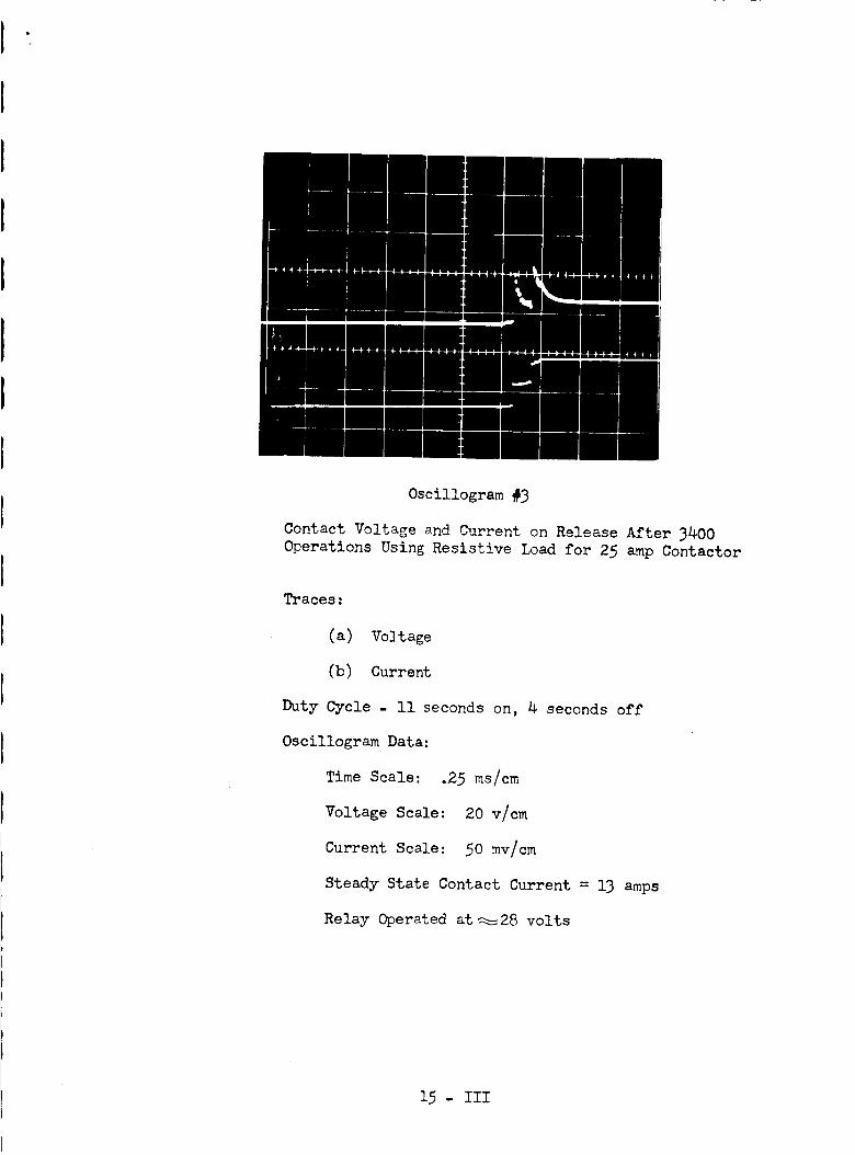
Oscillogram#3

Contact Voltage and Current on Release After 3400Operations Using Resistive Load for 25 ampContactor

Traces:

(a) Voltage

(b) Current

Duty Cycle - ll seconds on, 4 seconds off

Oscillogram Data:

Time Scale: .25 ms/cm


Current Scale: 50 zv/cm



15- III

!

Oscillogram #4

Contact Voltage and Current on Operate after 3400

Operations Using Resistive Load for 25 amp Contactor

Traces:

(a) Two sets of vo/tage on release

(b) Two sets of current on release

Duty Cycle - II seconds on _ seconds off

Oscillogram Data:

Time S,_ale: .25 ms/c_

Voltage Scale: 20 v/em




16 -III

Oscillogram _5

Contact Voltage and Current on Release After TenOperations Using Inductive Load for 23 ampContactor

Traces:

(a) Voltage

(b) Current

0scillogram Data:

Time Scale: l0 zs/cm


Current Scale: 2 v/cm

Current Shunt_.8_cold

Relay Operated ate8 volts.

17 -IIl

Oscillogram#6

Contact Voltage and Current on Release After Ten

Operations Using Inductive Load for 25 amp Con_actor

T_acs_ :

(a) Voltage

(b) Current

Oscillogram Data:

Time Scale: 10 ms/cm

Voltage Scale: 20 v/_m

Current Scale: 1 vfcm

Current Shunt_.25J_cold


18 -III

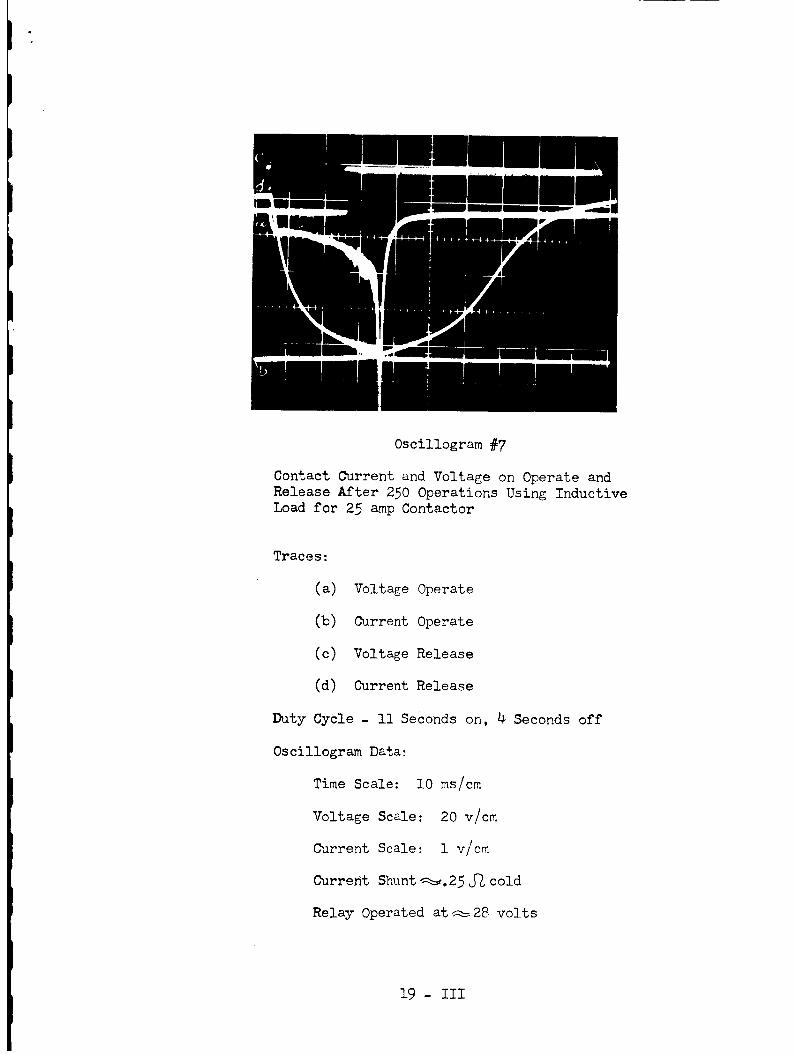
0scillogram #7

Contact Current and Voltage on Operate and

Release After 250 Operations Using Inductive

Load for 25 amp Contactor

Traces:

(a)

(b)

(c)

(d)

Voltage Operate

Current Operate

Voltage Release

Current Release

Duty Cycle - ll Seconds on, 4 Seconds off

Oscillogram Data:

Time Scale: l0 ms/cm


Current Scale: 1 v/cm

Current Shunt_.25j_cold


19 -III

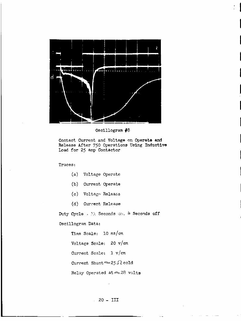
Oscillogram #8

Contact Current and Voltage on Operate and

Release After 750 Operations Using Inductive

Load for 25 amp Contactor

Traces:

(a)

(b)

(c)

(d)

Voltage Operate

Current Operate

Voltag_ Releas_

Current Release

Duty Cycle ,o?.i Seconds on_ h Seconds off

0scillogram Data:



Current Scale: i v/cm

Current ShuntS25 J_ cold

Relay Operated ate.28 volts

20 -III

L

SECTION II

CONTACT RATING

As mentioned previously, a test was conducted on a contactor whose con-

tacts were rated at 25 amperes. With a resistive load, no damage was evident

to the contactor. Since it was known that a cantilever spring which held

one contact of a pair had been welded under service conditions, an evident

question was, "What are the actual load conditions to which a contactor is

subjected?"

An answer to this question was that a contactor with a set of contacts

rated at 25 amperes, 50 amperes, 100 amperes or 200 amperes, could be sub-

Jected to practically every type of a load which was possible. In other

words, the current of the contact circuit could be caused by a resistance,

an inductance or a capacitance. On the contact load circuit, any or all of

these conditions could exist simultaneously and for varying times.

The contactor was expected to open and close circuits for all of the

varying conditions and in addition, open and close circuits for motors, lamps,

etc., when the foregoing situation existed. It was found, however, that the

mating contacts would only function for a relatively few cycles for a rated

current which was obtained from a highly inductive load. The terminals to

the contactor became excessively hot and under some conditions, the arc

across the contacts w_uld continue to exist for some time after the contacts

were separated. As would be ex_ected the contacts were damaged excessively.

The question then is, what is an adequate set of specifications for

electrical contacts? It is not expected to answer this question immediately,

however, some satisfactory solution must be found if contacts in electrical

contactors and in electromechanical relays are to preform under the conditions

enumerated. It is quite probable that the description of the duty of the

contacts is inclusive to the extent that this could serve as a final specifi-

cation but it does point to a glaring lack of information in this area.

l- II

In an attempt to outline the problem, the following outline was pre-

pared. While this is a preliminary outline, it does indicate that an

intelligent application of contacts must be made as well as an improvement

in the scheme used to rate contacts.

REQUIRED CONTACT SPECIFICATIONS

I. Stability

2. No chatter, I0 to 2000 cps, 20 g

3. Load on contacts

(a) Capacitive, inrush of current shall be no more than twice

rated current; time constant no greater than

(b) Inductive load with a time constant of less than

(c) State rated voltage, and whether it is DC or AC.

(d) Steady state current is equal to rated current.

_. Life -- duty cycle -- number of operations, contact resistance --

rated load -- temperature.

5. Temperature

6. Coil voltage - range - nominal - power supply internal impedance.

7. Sealed - leakage l0"e cc/sec.

Upper Bound

Operate timeRelease time

Coil power

WeightVolume

ower und

Insulation resistance

Dielectric strenEth

Some rational scheme to arrive at specifications for contact8 must be

used if contactors and relays are to be utilized satisfactorily. Of course,

the specifications alone cannot replace the proper application of these

devices. In other words, after proper contact specification has bee deter-

mined, the proper contactor must be used for a given Job. Not much has been

2- II

I

I

i

I

L

L

accomplished in this direction but the proper usage of equipment and devices

is a prime prerequisite if satisfactory functioning is to be expected.

It is quite probable that a special contact rating will berequired for

those places where a highly inductive current is to be interrupted. At the

moment, not much information is available for the closing of contacts for

incadescent lamp loads and motor loads. The meager data on hand seems to

indicate that the breaking of circuit carrying a highly inductive load is

the most severe case. If this is correct then, the problem resolves into

the specification and design of contacts for this case.

3- II

SECTIONIII

THEORETICALINVESTIGATION AND SOME EXPERIMENTAL

DATA FOR EI_CTRICAL CONTACT FAILURE CAUSED BY

ELECTRICAL LOADING

The interim report covering the period 1-1962 to 3-1962 indicated

the possibility of relating electrical load contact failures to arc

energy. This section presents the theoretical development of several

relationships based on ideas discussed in the preceding report. A

brief review of these earlier ideas and the modifications used in

this develo_aent are given before proceeding with the detailed de-

velopment.

The primary assumption discussed previously was that the proba-

bility for "failure" due to electrical load is related to arc energy.

This assumption is qualified in the ensuing work by restricting the

study to medium and large current carrying contacts, designed for

cycle duty, (i.e., not one shot relays.) For these type contact

systems, the following electrical contact system conditions are said

to constitute a failure under current load _ rated load.

(I) Prolonged arcing in the open position on break.

(2) Contact lead connections becoming faulty due to electrical

load heat generated by contacts.

(3) Contacts welded closed.

(4) Failure to establish electrical continuity on make.

I - llI

(5) Electrical discontinuity occurs during steady state load <

rated load, due to heating by ImR of the contact system.

(6) Contact system discontinuity failures induced by electricalcontact heat, not covered by (I) through (5), (i.e., springs

failing due to excessive heat, etc.).

Most of the above conditions are common electrical failures associ-

ated with cyclic contactors. An additional condition is now defined

which is somewhat unusual but is believed to have merit, along with

usefulness in the following analytical development. This condition is

called Condition A.

Condition A:

If all of the mass from either set of a contact pair is reduced by

the original amount then either (i) a condition of the type (1)

through (5) has occurred or (ii) the expected value of the proba-

bility for continued satisfactory operation is zero. Also, if no

mass from either contact is removed the probability of failure is

zero,

"Condition A" although open to criticism, allows a starting point

from which analytical relationships can be derived. If these relation-

ships prove useful _l failure estimatio_ and contact design, then

criticism of the hypothssis can be of a constructive n_*,ure.

Using the essence of "Condition A", the following concise assumption

is given.

For the probability of failure less than k, (Pr [f_ilure]<k),

there is a distribution of mass transfer, f(MT) such that:

(a) f(MT) is a continuous probabil _ty density function with the

properties given in (i)

2 - III

%) w_= mass transfer due to arc energy for the contact pair

ich monotonically loses mass under a given load condition,

such that the steady state current is < rated load current.

(c) MV = original mass of the above contact.

I

I

I

I

(1) _v'r°f(_)_ = _o>Pr[failure]0

if MT is in the range IO,MTo ]

f(_)_. 1. F(_)

o = F(MT) if MT < 0

1 = F(_) "if _ _ Mv

The above hypothesis leads to the investigation of the failure,

as defined earlier, as a function of the mass transfer. The exact

nature of this distribution can only be found by an infinite number

of tests which is an obvious impossibility. However, on the basis

that the distribution is not symmetrical, but is skewed in the in-

creasing MT direction and is a function of only one parameter other

than MV, the following density appears to have possibilities.

(2) g(MT;MV, Ps) - C(I-E Mv/_s"v) _O_MT _<MV

= O otherwise

iwhere C = _..

0s,'/°']0

I- _ MT/"VPs

which gives g(MT;M_,O s) = MV[I ÷ ps_PsE]/t_ ] _OL::MT_<MV

Also the above distribution has the monotonic property that if lx > _z,

then MT: >MTz , which certainly appears reasonable.

3 - III

The investigation to date on the correlation between _ss transfer

and arc energy indicates that MT might be approximated by the following

function. The data of Figures (I) and (2) indicates some results of

the investigation to date, and is discussed in more detail in connection

with using the results of the present development.

N T N

MT = CIA(I+ CsA) where A = arc energy = EiIid T = Aci

i=l o i=l

Aci = the arc energy of the ith arc period.

Toi = ith arc period.

E i = arc voltage during the ith arc period.

Ii = arc current during the ith arc period.

C1and Cs are constants which are presumed to be functions of the following

factors.

(a)

(b)

(c)

(d)

(e)

(f)

Average contact temperature during operation

Type of contact material

Contact pressure during closure

Impact pressures

Contact surface area

Sealed or unsealed and dielectric media alo_ W_t_ m_dia

pre ssure

(g) Gravity and electrical polarity.

To obtain the probability for failure in terms of arc energy A, the

following density transformation can be made.*

* "Introduction to the Theory of Statistics"

4 - III

Mood, McGraw-Hill

where

since

H(A;MV, Ps, Cx, Ca) = g(HT(A)) Id_l;A(O)< A < A(l_r )

A(O) = the value of A when MT = 0

A(NV) = the value of A when MT - MV

I_I = C_ (I + 2C=A) the above becomes

(3) H(A;_,PB,Cx,C=)-C, I(I+2CIA)[I - ECIA(I+C2A)/psMvl

.v[l *ps-.s

= 0 otherwise

where A has the limits

0 < A < 2-_I Cx

Also if the load cycle of a contactor is repetitive in nature, the

arc energy can be written as:

A =NA c

where N = number of operations

Ac = arc energy per operation.

Transforming the H(A) density to an h(N) density (N, the number of

operations) gives, using the same procedure as before:

Cx (i+ 2C=AcN)[I - E't_CIN(I÷AC2N)/Mv_]"C(4) h(N;Ps,C1,Cm,Ac) =

MYI l *Ps-"s

rL vC__j2AcC = L-- Cx .J

This implies the probability of failure is directly related to the

number of operations permitted.

In order to demonstrate the use of equation (4) consider the follow-

Ing illustration.

5 -III

Knowing the type of load for which a contactor is to be used and

assuming that it is repetitive, then Ac can be found. Also, for a

choice of relay the constants MV, C_ and C, can presumably be found.

The problem then is to determine the number of operations, No, such

that the probability of failure is less than _o" (Note that Ps is as

yet not known but is presumably a constant once it has been determined.

A method for finding Ps will be discussed later.) The above problem

can be stated as: Find NO such that

No

S h(N;Ps,C:, Cg,Ac)dN " _o > Pr [failure]o

carrying out the integration yields the following equality which must

be satisfied by NO.

O.Ao.o?._'o"...... I.,.ps p,Ei''''_''

letting u0 . C,N 0 [I+ CIAcNo]Ac/MvPs

_o[_.,_ ,,,v,,]

(5) gives J = Uo+ ! -6 uO o _ uo E 1/D s

_ _l/_o_,_ _,[l+ps P. ]%

Expression (5) does not have an explicit form for uo. However, the

following development yields an explicit form which is of practical

interest: noting that

- I+ Uo- _2" + ...._Uo

_Iv.s ,_- - _ [_..(Uo)]2

6 - III

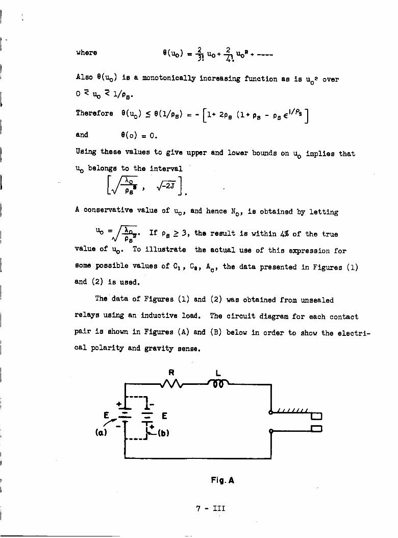
_. 2 =where eCuo) = Uo+ --_4.uo + ....

Also e(u o) is a monotonically increasing function as is uoS over

o _ uo _ 1/p s .

- Ps EIIPsThereforeO(uo}_<O(llPs)= -[i.2Ps(1.Ps ]

and e(o) = o.

Using these values to give upper and lower bounds on uo implies that

u0 belongs to the interval

A conservative value of Uo, and hence No, is obtained by letting

Uo =_. If Ps -> 3, the result is within 4% of the true

value of uo. To illustrate the actual use of this expression for

some possible values of CI , Ca, Ac, the data presented in Figures (I)

and (2) is used.

The data of Figures (i) and (2) was obtained from unsealed

relays using an inductive load. The circuit diagram for each contact

pair is shown in Figures (A) and (B) below in order to show the electri-

cal polarity and gravity sense.

R L

__V -r+ r-_

(A) t.__jl_(b) ]

Fig. A

7 -llI

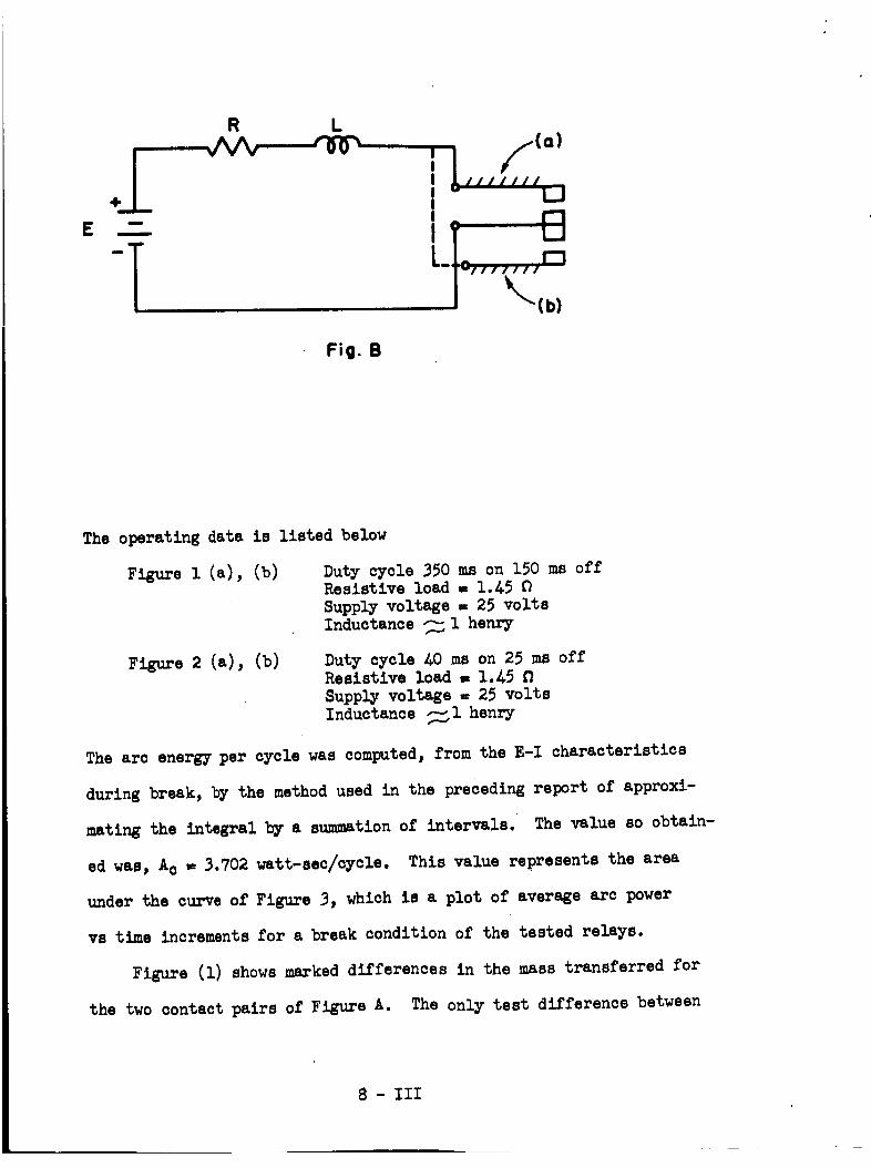
R

E mm

Fig. B

/,,-(a)

i ///

The operating data is listed below

Figure I (a), (b)

Figure 2 Ca), (b)

Duty cycle 350 ms on 150 ms off

Resistive load = 1.45 O

Supply voltage = 25 volts

Inductance _I henry

Duty cycle 40 ms on 25 ms off

Resistive load = 1.45

Supply voltage = 25 volts

Inductance _I henry

The arc energy per cycle was computed, from the E-I characteristics

during break, by the method used in the preceding report of approxi-

mating the integral by a summation of intervals. The value so obtain-

ed was, Ac = 3.702 watt-sec/cycle. This value represents the area

under the curve of Figure 3, which is a plot of average arc power

vs time increments for a break condition of the tested relays.

Figure (I) shows marked differences in the mass transferred for

the two contact pairs of Figure A. The only test difference between

8 - III

(a) and (b) of Figure A was the electrical polarity. Mass transfer was

considerably greater when the contact _s an anode than when it was

a cathode.

The two contact pairs of Figure (2) show similar mass transfer

characteristics although one is mass gained and the other is mass lost.

The main difference between the test conditions for Figures (I) and

(2) was the duty cycle and hence the average contact temperature. This

suggests that the main contributor to the mass transfer vs arc energy

relationship is temperature, for a g_ven contact material. (The fact

that temperature would influence the relationship is of course a

physical fact already known.) From Figure (i) the data suggests

that below a temperature region variables such as polarity and gravity

can be a noticable factor.

Assuming that the dotted lines through the data of Figures (I) and

(2) is representative of the Mr vs A relationship, and can be fitted by

the second order polynomial suggested earlier over the range of interest,

the constants C_ and Co will be evaluated using the formulas below.

01 mMTA _ - MTIA_m

AIAs _- A_

= mass at arc energy value As which has been transferred

= mass at arc energy value Am which has been transferred

C m =

Some care has to be exercised in selecting A1and As in order to

obtain a reasonable fit to the data, when the curve is other than a

9 -III

straight line. The constants were evaluated for curves (a) and (b)

of Figure (i) and (b) of Figure (2) using the circled points for AI

and A,. The constants are listed below.

Figure l(a) CI = (1.31)10 -4 gms/watt-sec.

Cs = -(.9)10 -6 per watt-sec.

Figure l(b) CI = (1.555)10-5 gms/watt-sec.

C, = -(.895)! 0-6 per w_tt-sec.

Figure 2(b) CI = (1.13)10 -3 gms/watt-sec.

C, = -(1.57)10 -6 per watt-sec.

Using the constants from Figure l(b) and Figure 2(b) along with the

value for MV of .5 gms the following e_mples are given using the

value of arc energy per cycle mentioned previously.

For Ao = 10-3 > Pr [failure] and using the conservative estimate

of uo gives /i0-3

U0 = _ ps8

using the definition of uo in terms of No gives

No = I I - I+2C_A c CI

which is difficult to evaluate when 4MvOsu°Cz << I

CI

However, by using the binomial expression and neglecting higher terms

than the first gives a good approximation. This technique will be used

for the data of Figure 2(b) and No becomes:

NoMVPsUo

AcC_

(Note: there is another value of

i.-----when Cs < 0ofN o at

+Cs

but this occurs after MT supposedly

has passed through MV)

I0 - III

or No_ (.5) _ = 38 operations(3.7)(I.13)I0-"

which says that for the load-duty cycle conditions imposed on the

relay tested in order for not more than 1 in lOs relays to fail the

relay should not be operated under these conditions for more than 38

operations. (This might seem like a severe restriction but it should

be kept in mind that the load on the relay contact pair of Figure 2(b)

was roughly I00 watts. Also both relays failed, due to burn out of

the original contact-to-terminal connections.) This occurred at about

4500 operations. Also in order for the temperature to stabilize with

a duty cycle of 900 cycle/rain., it is apparent that the transient

time for stabilisation is a contributing factor to the number of

operations until failure. In this light the above calculation implies

that this relay would not reliably operate with this load condition.

For the data of Figure l(a) and (b), the values of NO for _o = lO-s

are:

Figure 1 (a) = 326

Figure 1 (b) = 2730

These values indicate that for the duty cycle-load condition used,

(the load was the same as in Figure (2)) continuous operation should be

limited to 326 operations for the polarity of (a) and 2730 for the

polarity of (b). In a practical sense this number of operations still

suggests that the relays under test are not capable of reliable operation

using the load-duty cycle of the test conditions. This too was varified

by failure of connector straps after_ 300 min. of operation or

36,000 operations for 2 of 4 relays. Using Ao = 1/2 in the above

formula to predict the number of operations for Pr _ailur_ < 1/2 gives

ii -III

No _ 7400 for relay used in (a)

NO _ 60,000 for relay used in (b)

Although the above illustrations were based on limited data and

the proposed incomplete theory given earlier, the results suggest that

some useful practical expressions are possible by further development

of the proposed approach. Before discussing some of the possible

modifications to the proposed theory, a method for finding the "best"

estimator for the skew factor Ps is given. The method is based on the

statistical principle of "Maximum Likelihood Estimator".* The pro-

cedure is as follows:

Let (_I 'Mv,)_(MTs'Mv_ ).... (MTm,MVn) represent the original mass

and the mass transferred at failure for a random set of contactors

under random load conditions. (Steady state current must be __ rated

current. )

From the likelihood function

L = g_ (N%;P8,MV_)_(_;Ps,HV_ ) .... g_(_Tm;Ps,_. )

maximize L with respect to the skew factor Ps in terms of the measured

values of MTI and MVi. This gives the following expression which must

be satisfied by Ps.

n [ xi exd¢ ]I - Exil_s = n_i=l

PS + Ei/ps - PS £ilP_ ]

, f _JI * PS - ,PSEI/ps

where X i - MTJ Mvi

n = number of relays tested

* For reference see "Introduction to Theory of Statistics",

Mood, McGraw Hill.

12 - III

Although this expression is not simple: it is felt that due to the

possible results which could be obtained by having a good estimator for

Ps, effort should be given to solving the above. Also in order to check

the validity of the failure-mass transfer relation being independent of

the type of load, the above relationship could be evaluated twice using

two sets of data from two different types of load. To see the infI_ence

of the skew factor, Ps, on the probability distributions and the proba-

bility _, these are plotted in Figures 4 and 5 for several values of Ps.

As mentioned earlier this report is a first attempt at finding a

useful theoretical set of relationships which can be verified by experi-

mental data. In this area it goes without saying that this has not

been done to date. Although much work has been done in the physics

area of contacts, this work has not been integrated into analytical

relationships of the type being sought after by contact designers and

relay customers. 1'2 This is the goal of this particular investigation.

The first report gave only the basic point of view with which to attack

this problem. It is felt that the more concrete investigations (experi-

mental and theoretical) presented in this interim report indicate a

direction, and will be helpful in finding well founded expressions

with which to work.

Some of the possible modifications to the proposed theory are

discussed below and will be investigated further if future experimental

data so dictates.

I. "Electric Contacts" Ragnar Holms

2. "The Physics of Electrical Contacts" Llewellyn Jones

13 -III

I. The types of failure listed in (i) through (6) be re-

classified into one or more groups. This can be checMed by

the method indicated earlier for finding Pc.

If. Using a different expression to represent mass transfer

in terms of arc energy.

14- III

\\

\o

o;,U)

\\

\

0 _ 0

\

o_

,_, o _-

W

n_

_oO) \

01

_01 x

0

$1tIVI=IE) NI /SO'l 1=13.-ISNVldJ. SSVIN

15 - III

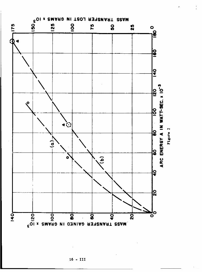
£0l x SNVI:IO0 m

NI kS01 1:II3--ISNVU.L SSVN

0 m 0N

0qrm

\

\

\\\

0

0

m

z___

0,It

0CU

o 0 o 0 o o0 m _ O q"m

;_ x S_IV_I9 NI (]3NIV9 _i:ldSNV_l£ SSVM

00

16 - Ill

L

I •

0tO

sL

0

o 0 0 o o

tn _ _ _ o

_.LIV_ NI .LN_IN3EIONI 31NI.L 9NIEII'IO EI3MOd OEIV

cO

iZm

-_ z

I--

M')

00 0

r._

17 - III

U'} 0r,i

Nm

0o _ o- d

II

X

r._

18 - III

IO

m

X

I I I Ill

x,Pl_,X) B AN/ =X

19 - III

0

LO

d

FURTHER DISCUSSION OF CONTACT FAILURE DUE TO ELECTRICAL LOADING

Report No. 3 Section No. III

In the report covering We peri_ I M_ch _62 to 30 April _62, a

method for fi_ing contactor failures caused _ electrical loading was

proposed. Be basic assumptions related contact failures to mass transfer

caused _ _ectrical load conditions. Mass transfer was then related

to arc ener_ich was in turn related to the number of operations for a

g_en duty cycle. _is report discusses several aspects _ich were

omitted or slig_ed in the preceding _port, along _th a more detailed

testing scheme _th which to test the proposed theol.

One of the important steps in being _le to predict the nu_er of

o_r_ions for a g_en prob_ility of faihre was that of relating mass

transfer to arc energy. Based on the results of sever_ tests it was

ass_ed that t_se _re related as:

_ = c_A(l + csA)

= mass transfer _e to arc energy for t_ contact pair which

monotonic_ loses mass _der a given load condition such

_at the ste_y state current is less than or equal to ther_ed current.

A = Total arc ener_ = _ lidT = Ac i

i=lo

Ac i = arc energy of ith arc period

Toi = ith arc period

Ei = arc voltage during ith arc period

Ii = arc current during ith arc period.

The constants ci and ca were presumed to be functions of:

(a) Average contact temperature during operation

(b) Type of contact material

I - III

(c) Contact pressure during closure

(d) Impact pressures

(e) Contact surface area

(f) Sealed or unsealed, dielectric media and media pressure

(g) Gravity and electrical polarit_

By lumping all of the above factors into the constants CAand Ca, the

analysis of failure was considerably simplified. However, by attacking

the problem in this manner, a considerable amount of testing would be

needed for a given relay, duty-cycle, environmental conditions, and

electrical load, before the constants c, and cz could be obtained with

which to predict failure. This is an undesirable situation when many

different applications are to be considered.

_h_opossible solutions to this problem based on experimental data

are presented in this report. Although both of these methods would

require a considerable number of tests it could be small comparedto the

amount of testing required for finding cA and cz for each different

application.

The first method for evaluating c, and cz is as follows:

(1) choose sets of co_patible primary values for the variables;

temperature, contact material (denoted in terms of constituents), media

(denoted in terms of constituents), media pressure, contact surface area,

sealed or unsealed and contact pressures. (Compatible is meant to be

the values of the above parameters commonlyused together in the range

of application.)

(2) Vary the parameters gravitational force and electrical polarity

between their extreme values.

This process would resuJt in a set of discrete ranges for the parameters

cA and c2 which could be u_ed to evaluate all applications which fell in

2 - III

one of these sets of ranges. Although this procedure would limit the

versatility and accuracy of the failure estimate relationship, it does

have the advantage of simplicity.

The second method for evaluating c: and cz is that of curve fitting.

This would require considerably more tests than the above method. However,

it offers a method for having ci and cz as analytic functions of the

important parameters mentioned earlier.

Since the evaluation of c: and cz as a function of their parameters

would only be considered subject to the validity of the failure theory,

further discussion of methods to accomplish this task will be postponed

until the validity is decided. These methods are discussed however, since

the first method mentioned, could be obtained when testing for the validity

of the mass transfer relationship.

The previous discussions assumedthat the mass transfer could be

related to arc energy by two constants ci and cz. The experimental

evidence to date has only indicated that this might be the case. A_so,

the test data to date indicates that in actuality, the data is far from

smooth. This presents the problem of calculating ci and cz from any

set of test data and interpreting the results. The following procedure

is suggested based on obtaining conservative values of ci and cs. That

is, obtaining values for cA and cs which gives a conservative value for

the number of operations for a given probability of failure. Also this

method offers a way to verify if the masstransfer arc energy relation-

ship can be approximated by the type relationship mentioned earlier,

using limited information.

In order for the probability distribution in terms of arc energy to

hold, the value of arc energy Ao when the masstransfer MT = MV is given

3 - III

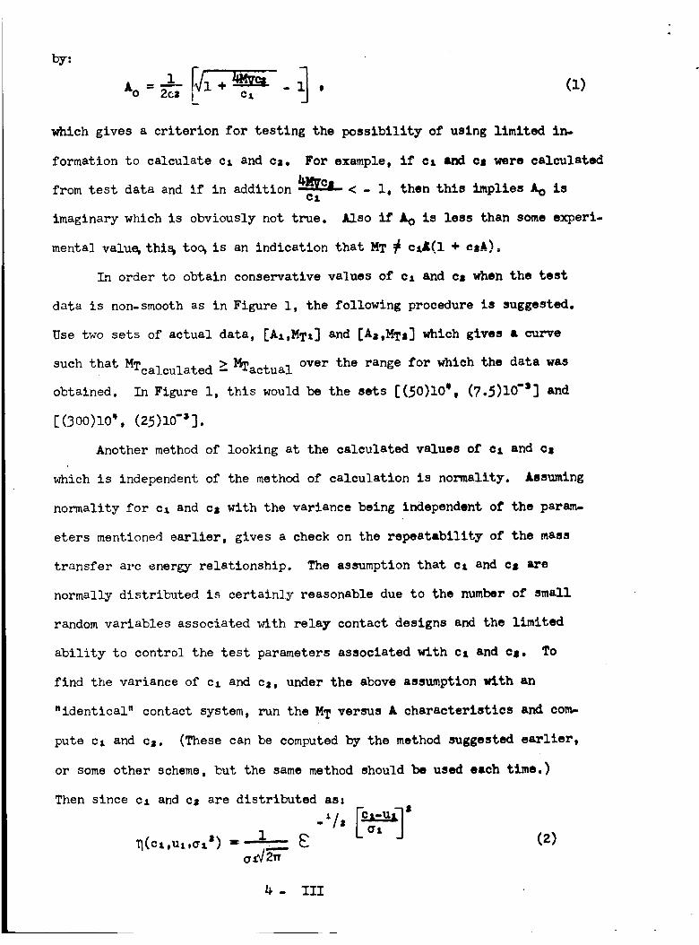
by:

which gives a criterion for testing the possibility of using limited in-

formation to calculate c, and ca. For example, if c, and cs were calculated

from test data and if in addition _ < - I, then this implies A O isci

imaginary which is obviously not true. Also if A O is less than some experi-

mental value& thi% to_ is an indication that MT _ ciA(l + e_,A)

In order to obtain conservative values of c, and cs when the test

data is non-smooth as in Figure I, the following procedure is suggested.

Use two sets of actual data, [AA,MT, ] and [Az,MT,] which gives a curve

such that MTcalculate d > MTactua I over the range for which the data was

obtained. In Figure I, this would be the sets [(50)10 e, (7.5)10"] and

[(30o)I0',(25)I0"3].

Another method of looking at the calculated values of cx and c|

which is independent of the method of calculation is normality. Assuming

normality for c, and c, with the variance being independent of the param-

eters mentioned earlier, gives a check on the repeatability of the mass

transfer arc energy relationship. The assumption that c, and cs are

normally distributed is certainly reasonable due to the number of small

random variables associated with relay contact designs and the limited

ability to control the test parameters associated with cx and cs. To

find the variance of c, and ca, under the above assumption with an

"identical" contact system, run the M T versus A characteristics and com-

pute c, and ca. (These can be computed by the method suggested earlier,

or some other scheme, but the same method should be used each time.)

Then since CA and ca are distributed asz

L°* j1.___ (2)

- III

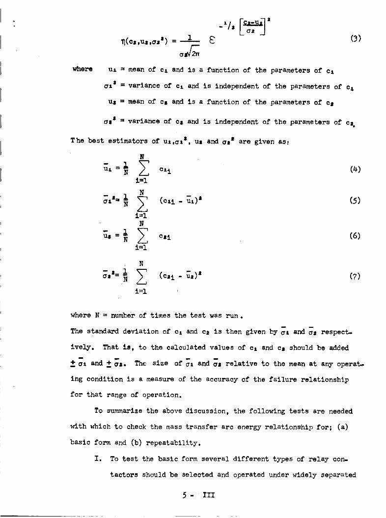
aW 2-

a

C3)

whe_ ul = mean of ci and is a function of the parameters of ci

al a = variance of ci and is independent of the parameters of cA

uz = mean of cs and is a function of the parameters of cs

_s s = variance of ca and is independent of the parameters of ca.

The best estimators of uA,al z, ul and aa s are given as:

N

111 =_N

i=l

N

i=l

N

i=l

(47

Cc:i- s (57

cai C6)

N

i=l

where N= number of times the test was run.

m

The standard deviation of ci and cz is then given by ax and _e respect-

ively. That is, to the calculated values of ci and cj should be added

_I and _ _z. The size of _I and _s relative to the mean at any operat-

ing condition is a measure of the accuracy of the failure relationship

for that range of operation.

To summarize the above discussion, the following tests are needed

with which to check the mass transfer arc energy relationship for; (a)

basic form and (b) repeatability.

I. To test the basic form several different types of relay con-

tactors should be selected and operated under widely separated

5 -III

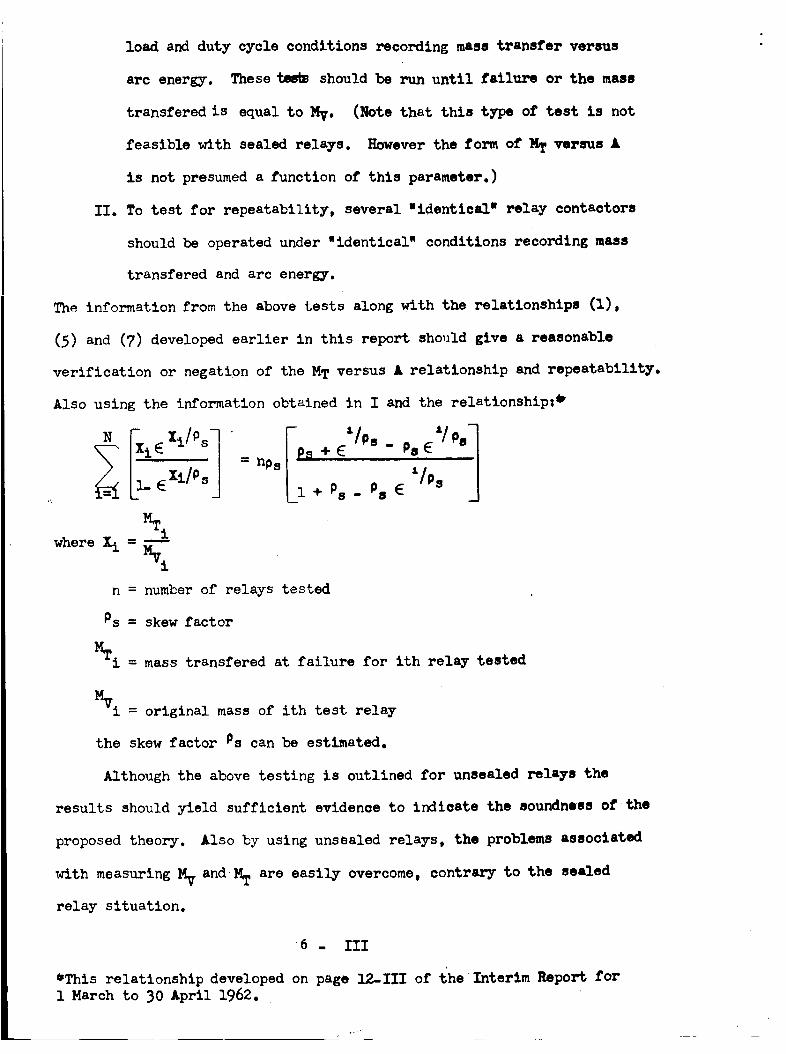
load and duty cycle conditions recording mass transfer versus

arc energy. These te_s should be run until failure or the mass

transfered is equal to MV. (Note that this type of test is not

feasible with sealed relays. However the form of MT versus A

is not presumeda function of this parameter.)

If. To test for repeatability, several "identical' relay contactors

should be operated under "identical" conditions recording mass

transfered and arc energy.

The information from the above bests along with the relationships (I),

(5) and (7) developed earlier in this report should give a reasonable

verification or negation of the MT versus A relationship and repeatability.

Also using the information obtained in I and the relationship: _

F.. z_./ps ' F V,,s. ,..."Ipsl

iE 1 n0s

_ __ _ Ip..,+ _ "a_- _ I

"/,, J

MT i

where Xi =_i

n = number of relays tested

Ps = skew factor

MTi = mass transfered at failure for ith relay tested

MVi = original mass of ith test relay

the skew factor Ps can be estimated.

Although the above testing is outlined for unsealed relays the

results should yield sufficient evidence to indicate the soundness of the

proposed theory. Also by using unsealed relays, the problems associated

with measuring Mvand _ are easily overcome, contrary to the sealed

relay situation.

•6 . III

eThis relationship developed on page 12-111 of the Interim Report for

1 March to 30 April 1962.

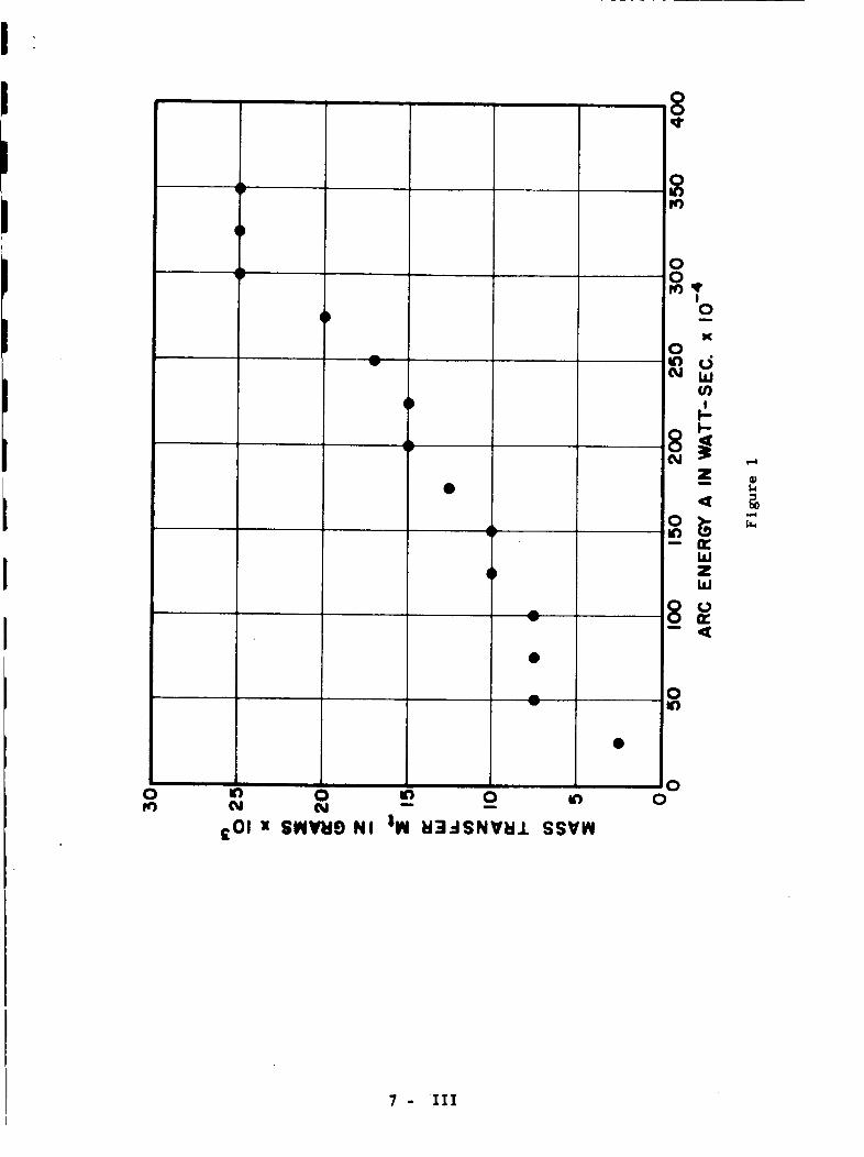
8

O

()

If)C_l

_01 x

()

AW

()

AW

Aw

O

SW_lr_O N I

1

IW W3_SNV_ SSVW

<I"

gI

oK

o

I

LI.IZLI.I

O

OO

7 - III

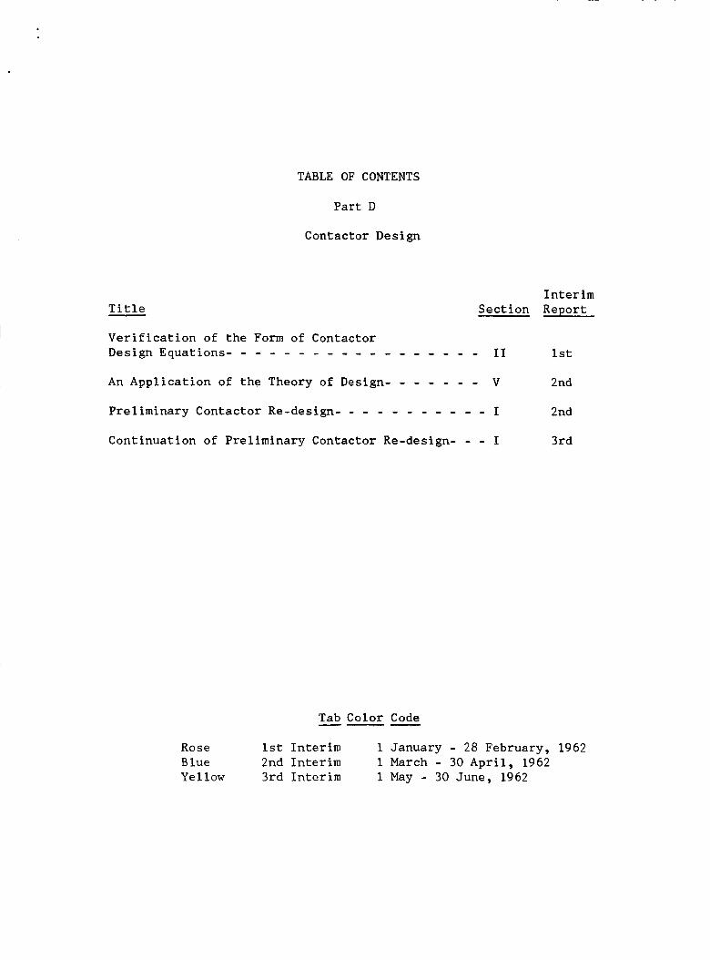
TABLE OF CONTENTS

Part D

Contactor Design

Title

Verification of the Form of Contactor

Design Equations ................ II

An Application of the Theory of Design ...... V

Preliminary Contactor Re-design ........... I

Continuation of Preliminary Contactor Re-design- - - I

Interim

Section Report

Ist

2nd

2nd

3rd

Rose

Blue

Yellow

Tab Color Code

ist Interim

2nd Interim

3rd Interim


I March - 30 April, 1962

i May - 30 June_ 1962

I ,

r

I

t

SECTION II

VERIFICATION OF THE FO_I OF Co_rACTOR DESIGN EQUATIONS

Several of the design equations developed in previous work were based

upon certain assumptions that were justified because of the nature of the

electromechanical device. Before these can be used in the design modifi-

cation of an electrical contactor, the accuracy of these must be deter-

mined.

Of the group of design relationships involved, only two or three have

to be verified, however, each one involves several variables. Some of the

variables involved are easily varied such as the supply voltage E and the

series resistance R. Other variables are difficult to v;_ry and require

that the contactor be open or unsealed to do this.

Two of the equations must be modified in order to predict accurately

the total seating time of the plunger. This exists because of the nature

of these contactors is such that compound spring action occurs during the

plunger closure. Because of the great change in the spring constant at

the point the power contacts make, the p_unger essentially stops and _aits

until additional magnetic pull is obtained before continuing its travel.

At room temperature and coll voltage slightly belo_v rated this additional

time caused by plunger hesitation is significant enough to have to be

considered on existing designs.

Since the manner in which different variables influence the function-

ing time of a contactor varies, it is necessary to define a variable that

_ill place the changes on a common reference. In addition this variable

should have some other desirable properties. One of these properties is

that, as this new variable approaches some limit, the functioning time of

the contactor should approach infinity (non-operate condition). In addition

l- II

it must contain the variables which influence the functioning time. The

most convenient variable found to date is defined as the ratio of the coil

pick-up current and the coil steady state current. The coil pick-up

current i_ is determined by the s_:me variables that determine the magnetic

flmx and the initial back tension on the plun_er. These variables are

the magnetic circuit reluctance, the coil turns and the initial plunger

back tension. These may be represented in various ways but let this ratio

of _,ick-up current to steady state current be a symbol h and called per

unit pick-up current. Then the following relation may be _iven.

i= = = (Xo+iss E E N _A '

Where: R t = total resist nce fre_ented to the _iplolv emf E (ohms)

E = supply emf in the Thevenins theore_l sense (volts)

N = total turns on the coil

Po = effective back tension on the plnn_er (ne_.,rtons)

x o = effective travel of the p]un_er of the magneticcircuit (meters)

= effechive non-_._orI<inC len:,_th of the m_i_gnetic circuit

in equivalent length of air (meters)

A = effective cross sectional area of the _4orking air ge.p

(square meters)

= permeability of free space (4n x lO _v t,rebers/amp - turn

meter)

An examination of equation (I) shows theft as the steady state current

(iss) approaches the magnitude of the pick-up current (ip) then the value

of h approaches one. From this definition when h approaches the value one 0

then the functioning time approaches infinity.

The plunger picI,_.up time (tp) is defined _s the time interval from

the instant the coil is energized until the magnetic pull on the plun_er

(1)

2- I!

equals the plunger back tension. At this time phonier motion commences.

In terms of the previous variables the pick-up time tp is given as

NS_A 1

tp : In

Since the supply voltage E only occurs in the variable h then when E is

varied tp should have the form

1

tp = C In I--'_

From the definition of the per unit pick-up current (h) can only have

useful values between 0 and 1. Figure 7, curve a, sho_s the form of equa-

tion 3. As h approaches 0 by varying E (E must approach infinity) the tp

approaches zero.

E Variable

To check the form of equation 3 requires that data be obtained of the

transient coil current build-up as a function of time _ith E as a vari-

able. These data are sho_n by the traces in Figures l, 2 and 3. Trace a,

in Figure 1 is for the highest voltage or smallest h value. The influence

of increasing h or decreasing E is shown by the next two traces b and c.

Traces a, b and c of Figure 2 show a continuation of decreasing E or in-

creasing h as well as those of traces a, b and c of Figure 3. Commencing

__th trace a, of Figure l, and progressing through from a to c on the

others and ending with trace c of Figure 3, covers the following values of

h; 0o418, 0.460, 0.500, 0.535, 0.657, 0.767, 0.822, 0.920 and 0.99.

Examination of the traces shows several thin_s ta]:in_ place as h is

increased by decreasing the supply voltage E. For the highest value of

E, _hich is the smallest value of h, the coil current essentially has one

smooth cusp. A small second cusp is evident. It is this second cusp that

suggests that the plunger is hesitating or stopping in its travel. As h

(2)

(3)

is increased by decreasing E this second cusp and its corresponding build-

up becomes longer in time. For some values of h this second build-up and

cusp sho_ some additional humps. This suggested some additional plunger

or contact rebound. This assumption is further verified by e}_amining the

contact voltage trace which is sh_,_n simultaneously along with the coil

current. In those cases where additional changes occur in the second

hump, definite contact chatter is recorded. This chatter is shown in the

_,u_u vu_b_ge trace as the short breaks in the horizontal traces. The

contact voltage trace also shows that the first cusp is definitely deter-

mined by the closure of the power contacts.

Since the time involved in the second build-up and cusp is a signifi-

cant portion of the total plunger seating time, it is desirable to account

for this in the design equations. The shape of the second _ild-up and

cusp suggests that this time interval consists of a second pick-up and

transit time. Since it is not experimentally possible to determine the

second pick-up current in these sealed contactors this must be determined

by solving two equations simultaneously. One of these equations is that

given by equation 3 and the other must be the equation of the plunger

transit time. From previous work the form of the armature transit time

equation is given as

_ere: M : effective mass of the plunger (kilograms)

x o = effective travel of the plunger of the magneticcircuit (meters)

R t : total resistance presented to the supply emf E (ohms)

E = supply emf in the Thevenin's theorem sense (volts)

h : per unit pick-up current (see equation I)

_- II

= effective non-working length of the magnetic circuit

in equivalent length of air (meters)

K = effective spring constant of the restoring spring

acting through the distance xo (newtons/meter)

Po = effective restoring force on the plunger existing atthe air gap xo (coil unenerglzed) (neutrons).

Since h is a function of E then when h is changed by varying E, the form

of equation 4 is

Curve a, in Figure 8, shows the form of k as h is changed by varying E.

Comparison of curve a, in Figure 7, and curve a, in Figure 8, shows that

the pick-up time tp and the transit time k have some similiar points at

h = 0 and h = 1 but in between the variations are somewhat different.

To verify the form of equations 3 and 5 requires that experimental data

of tp and k as a function of h be obtained. This is obtained from the

Figures l, 2 and 3 in the following manner. The actual value of pick-up

current is recorded, then knowing the current scale used _th the oscillo-

gram trace the time at which the current reaches the value is the pick-up

time. This is shown graphically in the follo_cing sketch.

i

iS;

Ip

I

/ I !/ u i a

I J

! J If I I

tp, k, tp2 k2

> t

5- II

(5)

If only one build-up and cusp exist then the subscript one will not be

needed or used. The pick-up current ip associated _th the first pick-up

time tp: is the only pick-up current that can be measured with these

contactors when they are sealed. If the contactor is open then it might

be possible to determine the second value of the pick-up current by set-

ting the plunger to a position corresponding to that of the second pick-

up point.

Table I shows the values of the pick-up and transit times as functions

of the variable h as E is varied. These values are obtained from measure-

ments made from the traces in Figures l, 2 and 3.

Table I Variable E

Figure-Trace h tp_ kl tpz + k_

ms ms ms

1 - a o.418 9.5 lO 3.51 - b 0.460 10.5 11.5 5.5

I - c 0.500 13,0 II.0 8.7

2 - a o.535 14.0 ll.5 lO.O2 - b 0.657 21.0 13.0 16.0

2 - c 0.767 29.0 17.5 25.0

3 - a 0.822 34.0 19.0 30.0

3 - b 0.920 49.5 29.5 42.0

3 - c 0.99 tp1+k1=215 65.0

The experimental values of tpl and kl are plotted in Figure 9 as

solid lines. The dashed lines are the results of using equations 3 and

5 _ith the value at h = 0.657 the same as the experimental. This is

equivalent of determining a value of C and D for each of the equations

by using the times measured at h = 0.657.

Only the sum of tpz and kz can be measured directly from the traces

since the second pick-up current can not be directly determined. If the

sum of tp2 and kz is plotted against hl in Figure 9, a smooth curve is

6- I!

obtained that has an apparent h axis intercept of hl = 0.333. This implies

that the h variable associated _th the second pick-up and transit must

be different from h:. Since as h: approches 1 both the first and second

cusps approach infinity then this suggests that hz approaches 1 as hl

approaches I. The h2 variable then can be related to the h: variable as

h, = 1.5h: - 0.5.

The sumof tp_ and kz is plotted against hz in Figure lO. A spot

check of the shape of curve a in Figure 7 with this curve shows that the

sumof tpz + ka is not a pick-up time function alone. Also a check of

curve a in Figure 8 shows that the sum of tp2 and k, is not a transit time

function alone. This implies that the function being sought consists of

two time intervals as the sum suggests. Let this sumof tpa and kz be

called the second seating time tsa as

ts2 = tpa + kz.

From equations 3 and 5 the form of equation 7 is

= Czln ll.hz + Dz ( )ts,

Since this equation involves _<o unknowsat least two sets of values of

ts2 and hz must be used. Using the pair tsa = 6.3, ha = 0.2 and the pair

ts, = 34, h, = 0.8 gives Ca = 17.32 and D2 = 3.87. Using these values of

Cz and Dz the second plck-up time tpz and the second transit time kz can

be calculated as functions of h,. The computedvalues of tp, and kz are

plotted in Figure I0. The computedvalue of tsa is plotted as the dashed

line in Figure I0 and follow the experimental curve (solid line) fairly

close. Since the transit time seemsto be, in general, a small percentage

of the total seating time, the form of this seating time could be approx-

imated by equation 3 with h, = ha.

(6)

(7)

7- II

From the previous explanation the total seating time t s of the plunger

as a function of h, when h is changed by varying E, can be represented as:

where: ha = the ratio of the first Fick-up current to the sleady state

coil current. The first pick-up current is measuredby

determining the smallest value of coil current which _._II

result in complete closure of the plunger.

hz = the ratio of the second pick-up current to the steady state

coil current. The second pick-up current in most cases can not

be measureddirectly for a sealed device. If the device is open

then the second pick-up current is the coil current that v_ll seat

the plunger v_en the plunger back stop is set so that the NOpower

contacts are just touching. For a sealed device the value of hl

at which the second cusp just vanishes is used in the follo_Ting

equations as hi'.

hz = ahl + b _mere: a = I/(_-h1') and b = -h1'/(l-h1')

to obtain h2 as a function of h_. Since hl is directly measur-

able the h2 can be determined in terms of h_ as h2 = ahl + b.

Equation I0 then gives the form for the total seating time t s as a function

of the variable hl Wen hl is changed by varying the supply voltage E.

If. only one cusp exists then the equation for the total seating time, when

hl is varied by changing E, is simplified to

ts_ = C_ In 1-_-_I+ DI -n

R Variable

Equation 1 shows that h may be changed by varying the total series

resistance Rt. Equation 2 shows that the pick-up time tp is a function

8 - II

of both h and Rt. If equation 2 is rearranged so that Rt is written as a

function of h, then the form of the pick-up time equation becomes

when h is varied by changing Rt.

form of equation 12. This shows that the pick-up time can not approach

zero by changing R to zero. To verify the form of equation 12, traces of

coll current build-up _,&th variable Rt were recorded. These traces are

sho_n by Figures 4, 5 and 6. The top trace in each oscillogram is for the

smallest value of h and increases for the next trace down. Starting _&th

the top traces of Figure 4 and progressing down in each oscillogram through

Figure 5 and 6 the values of h are approximately 0._, 0.5, 0.6, 0.7, 0.8,

0.83, 0.9, 0.95 and 0.99. At the lowest value of h, which is also the

smallest Rt, the coil current build-up consists of essentially one smooth

cusp. As h is increased a second hump and cusp appear and the time in-

volved with this second hump increases with increasing Rt. A direct com-

parison of the variation of this second hump and cusp _,ith those of the

traces in Figures l, 2 and 3 is not possible since a different 25 ampere

contactor had to be used to obtain the influence of Rt on the functioning

times of the contactor. This change was necessary because the character.

istics of the first 25 ampere contactor _r_changed during a contact load

run when the contacts were over-heated. It appears that the spring used

to hold the moving contact on the plunger was annealed during the particu-

lar contact load run. The contactor involved has not been unsealed yet

because other tests are to be run on it before breaking the seal. Final

evaluation of this overheating will be made after the contactor is unsea]ed.

The data obtained from Figures 4, 5 and 6 are plotted as curves in

Figure II and are shown in Table II. The two solid lines are plots of the

(12)

Curve b of Figure 7 sh_¢s a plot of the

9- II

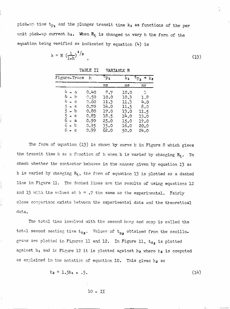
pick-u? time tpl and the plunger transit time k: as functions of the per

unit pick-up current hl. WhenRt is changed to vary h the form of the

equation being verified as indicated by equation (4) is

k = H (_I--_)_/3 (13)

TABLE II VARIABLE R

Figure-Trace h tp_ kl tpz + k2

mS ms mS

- a 0.40 8.7 I0.0 i

4 - b 0.50 lO.O 10.3 1.8

4 - c 0.60 11.3 11.3 4.0

5 - a 0.70 14.0 ll.5 8.0

5 - b 0.80 17.0 13.0 ll.5

5 - c 0.83 18.5 14.0 13.0

6 - a 0.90 25.0 15.0 17.0

6 - b 0.95 35.0 16.0 20.0

6 - c 0.99 62.0 50.0 24.0

The form of equation (]-3) is shown by curve b in Figure 8 which gives

the transit time k as a function of h when h is varied by changing Rt. To

check whether the contactor behaves in the manner given by equation 13 as

h is varied by changing Rt, the form of equation 13 is plotted as a dashed

line in Fizure ll. The dashed lines are the results of using equations 12

and 13 with the values at h = .7 the same as the experimental. Fairly

close comparison exists between the experimental data and the theoretical

data.

The total time involved with the second hump and cusp is called the

total second seating time tsz. Values of tsz obtained from the oscillo-

grams are plotted in Figures II and 12. In Figure II, ts2 is plotted

against hl and in Figure 12 it is plotted against h2 where h2 is computed

as explained in the notation of equation I0. This gives h2 as

h2 = 1.5hi - .5. (14)

I0- II

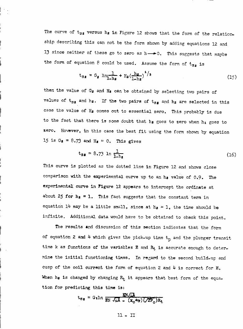
The curve of ts_ versus h= in Figure 12 shows that the form of the relation-

ship describing this can not be the form shownby adding equations 12 and

13 since neither of these go to zero as h---_O. This suggests that maybe

the form of equation 8 could be used. Assumethe form of ts, is

_hi_ (15)ts_ = Gz lnl--_lhz + HZ(l.hz)

then the value of Gz and H, can be obtained by selecting two pairs of

values of ts, and hz. If the two pairs of tss and hz are selected in this

case the value of H= comes out to essential zero. This probably is due

to the fact that there is some doubt that h, goes to zero when h, goes to

zero. However, in this case the best fit using the form shown by equation

15 is Gj = 8.73 and Hz = 0. This gives

1 (16)tss = 8.73 In l-h---_

This curve is plotted as the dotted line in Figure 12 and shows close

comparison with the experimental curve up to an hz value of 0.9. The

experimental curve in Figure 12 appears to intercept the ordinate at

about 25 for h, = 1. This fact suggests that the constant term in

equation l_ may be a little small, since at hz = l, the time should be

infinite. Additional data would have to be obtained to check this point.

The results and discussion of this section indicates that the form

of equation 2 and 4 which gives the pick-up time tp and the plunger transit

time k as functions of the variables E and Rt is accurate enough to deter-

mine the initial functioning times. In regard to the second build-up and

cusp of the coil current the form of equation 2 and 4 is correct for E.

When hj is changed by changing Rt it appears that best form of the equa-

tion for predicting this time is:

ts, = G,in _ j-_. (xo_M=)(_o)R t

II- II

where: E = supply emf in the Thevenin's theorem sense (volts)

N = total turns on the coil

u, = permeability of free space (4_ x 10 -7 weber/ampere-turn

meter)

A = effective cross sectional area of the working air gap

(square meters)

x o = effective plunger travel existing when power contactsare just touching (meters)

= eff_cLive non-working length of the magnetic circuit in

equivalent length of air (meters)

Po = effective back tension on the plunger when power contact

are just touching (new,tons)

Rt = total resistance presented to the supply E (ohms)

Ga = a constant determined at present by Gz = ts2/In(I/l-hz)

_ere tsz and hz are a measured pair of values.

If the second build-up and cusp seem to be a desirable characteristic

of the contactor operation then addibional development would need to be

undertaken along the line of predicting the pick-up time v_en the coil is

carrying a bias current. At present the second build-up and cusp is not

considered necessary or desirable.

12- II

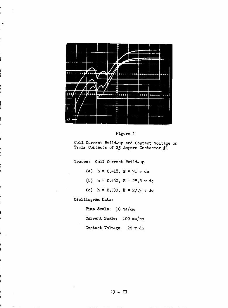
Figure I

Coll Current Build-up and Contact Voltage on

T:-L: Contacts of 25 Ampere Contactor #l

Traces:

(a)

(b)

(o)


h = 0._18, E = 31 v dc

h = 0.460, E = 28.8 v dc

h = 0.500, E = 27.3 v dc

OscillogramData:


Current Scale: lO0 ma/cm

Contact Voltage 20 v dc

13 - II

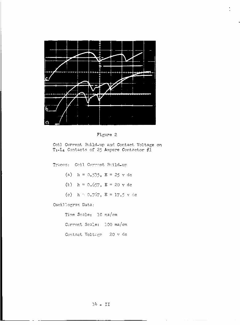
Figure 2

Coil Current Build-up and Contact Voltage on

TI-LI Contacts of 25 Ampere Contactor #I

Traces:

(4)

(b)

(c)

Coil C_rrent _ild-up

h = o.5_5, E = 25 v dc

h = 0.657, E = 20 v do

h = 0.767, E = 17.5 v dc

Oscillogram Data:

Time Scale: lO ms/cm

Current Scale: I00 ma/cm

Contact Voltcge 20 v dc

14 - II

Figure 3

Coil Current Build-up and Contact Voltage on

Ti-L: Contacts of 25 Ampere Contactor #l

Traces :

(a)

(b)

(c)


h = 0.822, E = 16 v dc

h = 0.920, E = I_.I v dc

h = 0.99, E = 13.2 v dc

OscillogramData:

Time Scale:

Current Scale:

Contact Voltage

Traces a & b, 20 ms/cm

Trace c, 50 ms/cm

lO0 ma/cm

20 vdc

15- II

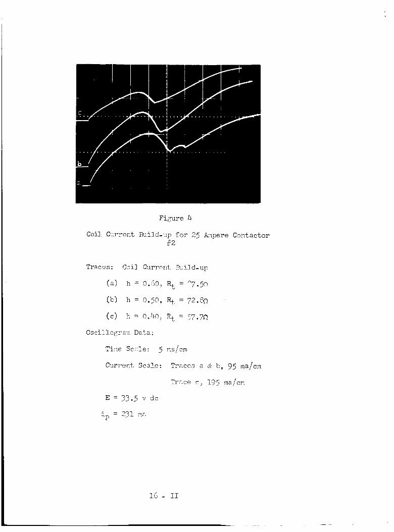
Figure 4

Coil Current Build_up for 25 Ampere Contactor

#2

Traces :

(a)

(c)

Coil _rrent Duild-up

h = 0.601R t = _7.50

h = 0.50, R t = 72.80

h = 0._0_ R t = 57.7_

Oscillocram Data:

Time Scale: 5 ms/cm

C_irrent Scale: Traces a _ b, 95 ma/cm

Trace c_ 195 ma/cm

E = _.5 v dc

ip = 251 ma

_G- iI

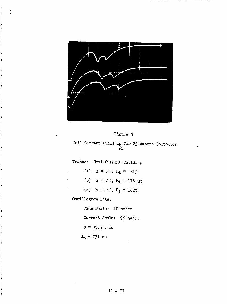
Figure 5

Coil Current Build-up for 25 Ampere Contactor

#2

Traces:

(a)

(b)

(c)


h = ._3,at = 1210

h - .80, at = 116.5n

h-- .?0,_t = lO2n

Oscillogram Data:

Time Scale: lO ms/cm

Current Scale: 95 ma/cm

E = 33.5 v dc

= 231 ma

17 - II

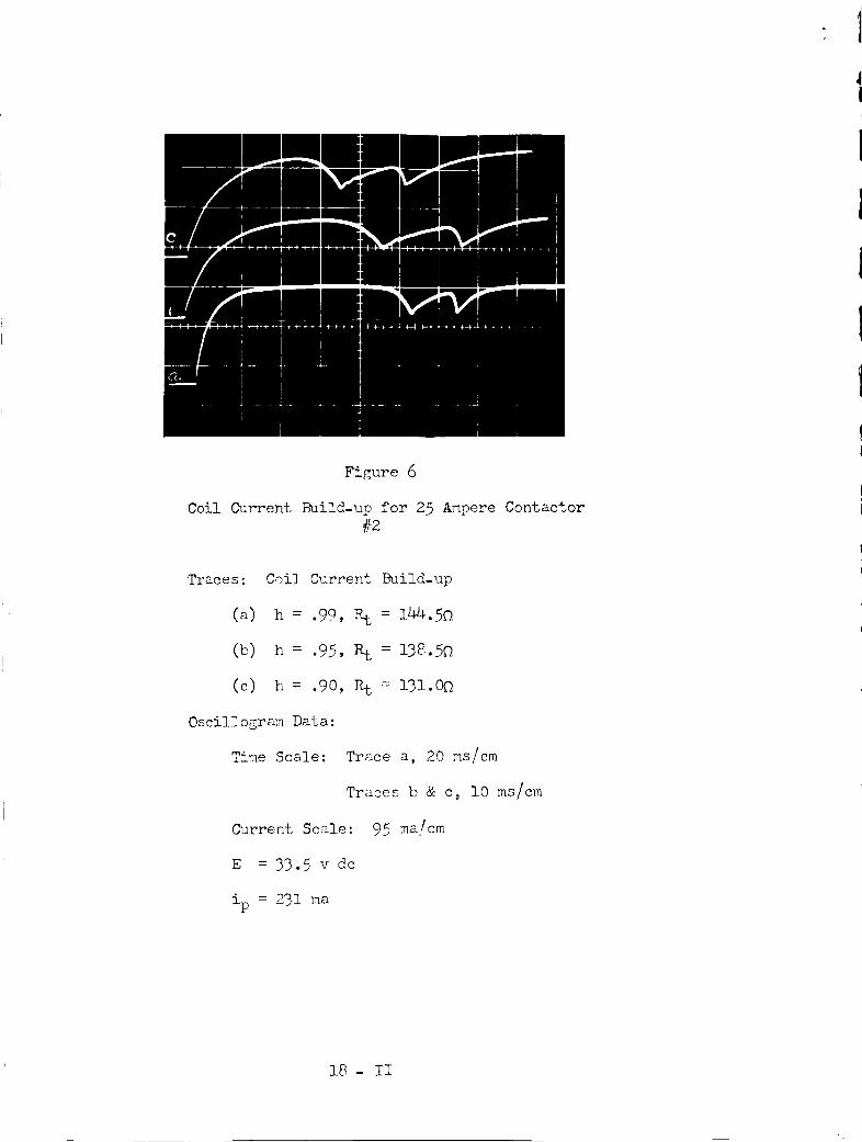
Figure 6

Coil Current Build-up for 25 Ampere Contactor

#2

Traces:

(a)

(b)

(o)


h = .99, Rt = 144.5_

h = .95, Rt = 1_8.5_

h : .90, _ = 131.00

Oscillogram Data:

Time Scale:

Current Scale:

E = 33.5 v dc

Trace a, 20 ms/cm

Traces b & c0 I0 ms/cm

95 ma/cm

ip = 231 ma

18- II

0

h'}, i

W} {U

v

W {.}

!

_w

0

I°o

dD,

4.J

v

r 0

I"

_w(U

oZ

d

bO

o0

19 - II

io 0 _ 0

\ \

.I,0

:D¢J

I:Ib,l

0

v

,.IJ

(D

0

I

GOd

I-i

i_. m.,

d.IJ

i,i-io

_0 od ,IJ

¢J

_ t _

d _

d °

oZ

o. _o o_ 0

0

0o

20 - II

0

-. %\

y

0 o o o oit) _ I_ tM

0

mc_

0

d

d

cJ

it)d

d

m

d

00 0n

S uul,- _s/, , ')I ' 'd_,

t

J-40

0

.IJ

0

0U_

v-4

o

o

o

¢xl

o

N _

21 - II

0 0 0 0 0 0 0IW. _) Ic) _1" I¢) _1 --

0

0

0J

00

4-J

0

0e-I

22 - II

I i i

0 0 0 0

d

m

d

' 000

23 - II

O

-%

O Opr)

O O

O

('4

4-*

O

d =

4.JAJ

Q)

dO4

q-4O

od

O

d r"

('4cn

q-4

O

r0

d

N

d

d

OO

,-4

a)

O

0

m

("4

1.4

24 - II

ANAPPLICATION OF THE THEORY OF DESIGN

BY

C. F. Cameron, Professor of Electrical Engineering

D. D. Lingelhech, Assoc. Prof. of Electrical Engr.

C. C. Freeny, Instructor of Electrical Engineering

R. M. Penn, Instructor of Electrical Engineering

Oklahoma State University

8tillwater, Oklahoma

FOR PRESENTATION AT

THE TENTH NATIONAL CONFERENCE ON ELECTROMAGNETIC RELAYS


OKLAHOMA STATE UNIVERSITY

STILLWATER, OKIAHOMA

April 24, 25, 26, 1962

ANAPPLICATIONOFTHETHEORYOFDESIGN

by

C. F. Cameron, Professor of Electrical Engineering

D. D. Lingelbach, Assoc. Prof. of Electrical Engr.

C. C. Freeny, Instructor of Electrical Engineering

R, M. Penn, Instructor of Electrical Engineering

Oklahoma State University

Stillwater, Oklahoma

INTRODUCTION

A concept is necessary before a desSgn can be started. It is usual toconceive of a model which has the desired characteristics. Most often the

physical device which is constructed is somewhat different than the concep-

tion of the mental model. There maybe many concepts whichareimpossible

to translate into physical reality. To assist in the process of translation

from a mental model to a physical object, the process known as design isutilized.

Synthesis is the combining of separate elements of thought into a whole

or a combination of elements into a completed unit. Analysis of a device orunit maybe accomplished after the device is finished. It is seen that

analysis is the opposite of synthesis. Design implies that synthesis follows

some logical procedure according to a plan and in some instances the designinvolves the formulation of a logical plan which maybe followed in the

building up of the elements which compose the whole or device.

I

Many schemes have been developed whereby physical devices maybe studied

by analytical means. A knowledge of the physical laws which govern a given

device makes it possible toanalyze the interrelation of electrical, mech-anical, thermal and other characteristics which a device exhibits under

certain conditions.

The realm of synthesis and desig_ have not been explored sufficiently

to have logical procedures which maybe used in the building up process.

Intuition seems to have been the process most often used to transformthe

concept into physical reality. Very frequently, the translation process has

been accompanied by much trial and error or cut and try.

It is the purpose of this paper to investigate a scheme which maybe

used in the design of a device after some indication has been given of param.

eters which must be fixed. The indication of the fixed parameters is inter.

twined with synthesis and design. The fixing of a set of parameters is

called fixing a set of specifications. Calling for a given set of specifi-

cations implies that the specifier knows what he needs which may not alwaysbe the case.

-I-

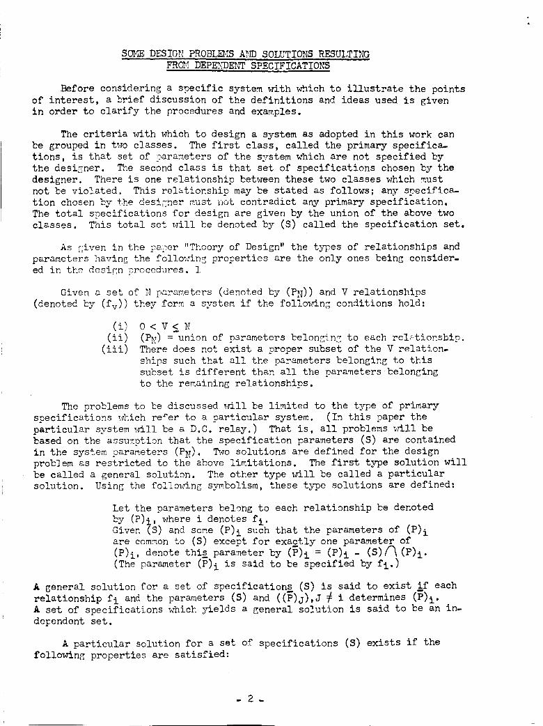
S(_._ DESIGN PROBL_}_ A}D SOLUTIONS RESULTING

FR@_ DEP_,DEh_ SPECIFICATIONS

Before considering a specific system with which to illustrate the points

of interest, a brief discussion of the definitions and ideas used is given

in order to clarify the procedures and examples.

The criteria with which to design a system as adopted in this work can

be grouped in two classes. The first class, called the primary specifica-

tions, is that set of oarameters of the system which are not specified by

the designer. The second class is that set of specifications chosen by the

designer. There is one relationship between these two classes which must

not be violated. This relationship may be stated as follows; any soecifSca-

tion chosen by the designer must not contradict any primary specification.

The total specifications for design are given by the union of the above two

classes. This total set _,rill be denoted by (S) called the specification set.

As given in the pa_er "Theory of Design" the t_qoes of relationships and

parameters having the followiny_ properties are the only ones being consider-

ed in the design procedures. 1

Given a set of N parameters (denoted by (PN)) and V relationships

(denoted by (fv)) they form a system if the follo_ing conditions hold:

(i)

(iii)

0 < V < N

(PN) = union of parameters belonzing to each rel_tionship.

There does not exist a proper subset of the V relation-

ships such that all the parameters belonging to this

subset is different than all the parameters belonging

to the remaining relationships.

The problems to be discussed will be limited to the type of primary

specifications which refer to a particular system. (In this paper the

particular system _II be a D.C. relay.) That is, all problems _,_II be

based on the assumption that the specification parameters (S) are contained

in the system parameters (PN)" _vo solutions are defined for the design

problem as restricted to the above limitations. The first type solution will

be called a general solution. The other type trill be called a particular

solution. Using the following symbolism, these t}_e solutions are defined:

Let the parameters belong to each relationship be denoted

by (P)i, where i denotes fi.

Given (S) and some (P)i such that the parameters of (P)i

are common to (S) except for exactly one parameter of

(P)i, denote this parameter by (_)i = (P)i - (S)/_(P)i"

(The parameter (_)i is said to be specified by fi')

A general solution for a set of specification£ (S) is said to exist i_f each

relationship fi and the parameters (S) and ((P)j),J # i determines (P)i"

A set of specifications which yields a general solution is said to be an in-

dependent set.

A particular solution for a set of specifications (S) exists if the

following properties are satisfied:

- 2.

(i)

(ii)

Each specifica$ion of (S) is a range of values for a

parameter of the system.

The system parameters common to (S) are in the range of

values specified by (S).

To illustrate the difference between a particular solution and a general

solution the following example is given for a relay system. The system is

represented by the matrix in Figure (I) where the N parameters are listed

vertically and the V relationships horizontally. The identification of the

parameters and relationships is given below:

6 = diameter of bare wire

= designstability point

Rp = reluctance of magnetic circuit presented to the coil with• the armature in the pick-up position

E = open circuit supply voltage (D.C.)k = armature transit or travel time

K = effective spring constant of spring system

= coil length

M = effective armature mass

N = coil turns

P = total power (steady state) supplied to relay coil circuit

by voltage source

Po = back tension at pick-up

Rc = coil resistance

Rt = total resistance of relay coil circui% presented to volt-

age source

Rs =R t . Rcs = outside coil diameter

tt_s= armature pick-up time= armature seating time

xo = armature air gap_A = (permeability of free space)(effective cross sectional

area of working air gap)

,f, = stability equation

fa = pick-up time equation

fs = transit time equation

f4 = power equation

fs = circuit resistance equation

f6 = coil resistance equation

fv = coll turns equation

fe = stability inequality

f, = magnetic circuit equation

f,e = pole face equation

f** = total time equation

In addition to the above N parameters and V relationships the following quan-

tities are involved when using the above relationships, however, they are not

considered parameters because of their restricted range of values.

B = ratio of core diameter to outside coil diameter

p = resistivity of conductor material= air equivalent of non-working part of the magnetic circuit

when using a series representation

-3-

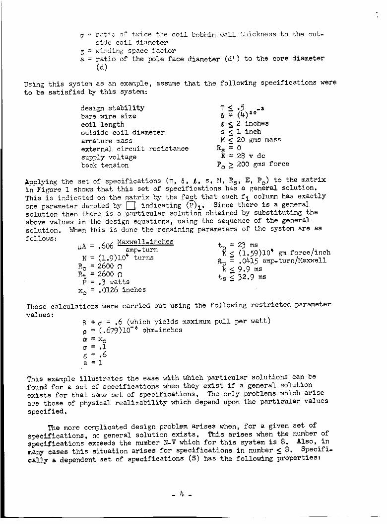
q = ratio of t_ice the coil bobbin wall thickness to the out-

side coil diameter

g = winding space factora = ratio of the pole face diameter (d') to the core diameter

(d)

Using this system as an example, assume that the following specifications were

to be satisfied by this system:

design stabilitybare wire size

coil lengthoutside coil diameter

armature mass

external circuit resistance

supply voltageback tension

8 = to

L < 2 inches

s _ 1 inch

M _ 20 gms mass

Rs=0E = 28 v dc

Po _ 200 gms force

Applying the set of specifications (_, 8, _, s, M, Rs, E, Po ) to the matrix

in Figure 1 shows that this set of specifications has a general solution.

This is indicated on the matrix by the fact that each fi column has exactly

one parameter denoted by [] indicating (_)i" Since there is a generalsolution then there is a particular solution obtained by substituting the

above values in the design equations, using the sequence of the generalsolution. When this is done the remaining parameters of the system are as

follows:_A = .606 Ma_,zell-inches

amp-turnN = (1.9)10 _ turns

Rc = 2600 O

Rt = 26O00P = .3 watts

xo = .0126 inches

= 23 mst_ <- (1.59)10' gm force/inch

= .0415 amp-turn/Maxwelleo < 9.9 ms

ts < 32.9 ms

These calculations were carried out using the following restricted parameter

values:

B + _ = .6 (which yields maximum pull per watt)

p = (.679)10 -6 ohm-inches

=X O

= .1

g = .6a = 1

This example illustrates the ease with which particular solutions can be

found for a set of specifications when they exist if a general solution

exists for that same set of specifications. The only problems which arise

are those of physical realizability which depend upon the particular values

specified.

The more complicated design problem arises when, for a given set of

specifications, no general solution exists. This arises when the number of

specifications exceeds the number N-V which for this system is 8. Also, in

many cases this situation arises for specifications in number _ 8. Specifi-

cally a dependent set of specifications (S) has the following properties:

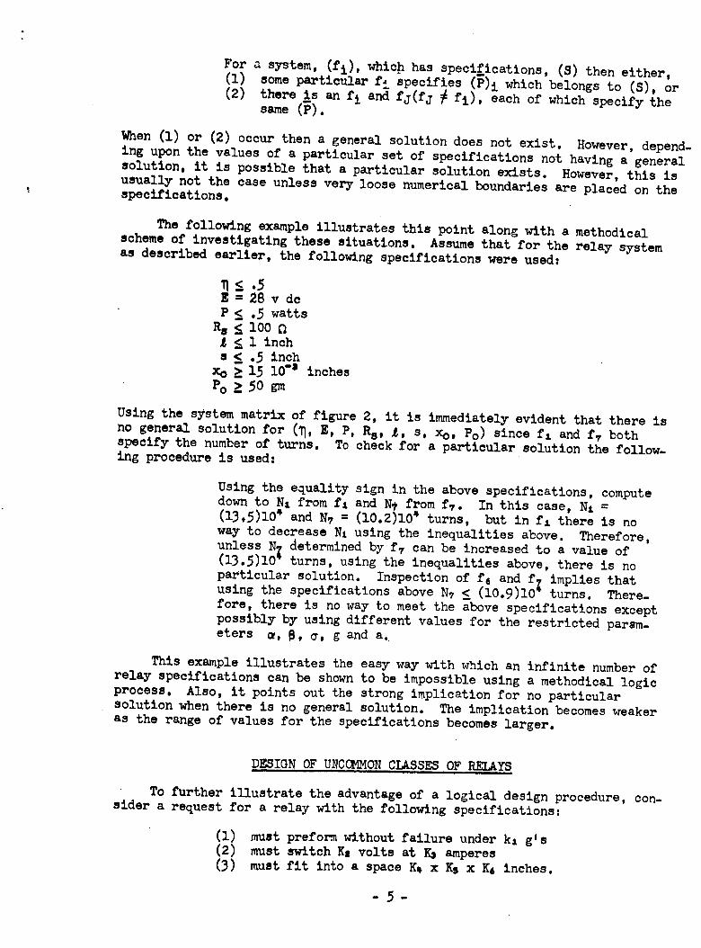
For a system, (fi), which has specifications, (S) then either,(I) someparticular f_ specifies (P)i which belongs to (S), or(2) there is an fi and fj(fj _ fi), each of which specify the

same(_).

When(I) or (2) occur then a general solution does not exist. However, depend-

ing upon the values of a particular set of specifications not having a general

solution, it is possible that a particular solution exists. However, this is

usually not the case unless very loose numerical boundaries are placed on thespecifications.

The following example illustrates this point along with a methodical

scheme of investigating these situations. Assume that for the relay system

as described earlier, the following specifications were used:

<_ .5E = 28 v dc

P <_ .5 watts

Rs < I00 n

<_ I inch

s <_ .5 inchxo _ 15 I0"s inches

Po _50 gm

Using the system matrix of figure 2, it is immediately evident that there is

no general solution for (_, E, P, Rs, _, s, Xo, Po) since f: and fv bothspecify the number of turns. To check for a particular solution the follow-

ing procedure is used:

Using the equality sign in the above specifications, compute

down to N, from f, and N$ from fT. In this case, N, =(13,5)10 4 and N_ = (10.2)10 4 turns, but in f, there is no

way to decrease N, using the inequalities above. Therefore,

unless N7 determined by f7 can be increased to a value of(13.5)10" turns, using the inequalities above, there is no

particular solution. Inspection of f6 and f7 implies that

using the specifications above N_ _ (I0.9)I0" turns. There-

fore, there is no way to meet the above specifications except

possibly by using different values for the restricted parsm-

eters 4, 8, s, g and a.

This example illustrates the easy way with which an infinite number of

relay specifications can be shown to be impossible using a methodical logic

process. Also, it points out the strong implication for no particular

solution when there is no general solution. The implication becomes weakeras the range of values for the specifications becomes larger.

DESIGN OF UNCOMMON CLASSES OF RELAYS

To further illustrate the advantage of a logical design procedure, con-

sider a request for a relay with the following specifications:

(I) must preform without failure under kl g's

(2) must switch Ks volts at Ks amperes

(3) must fit into a space K4 x Ks x Ki inches.

-5-

00[30E]FI00E][3O[3[300[3[3[3[Z]

8

Illp

E

k

i<

M

N

P

Po

Ro

Rt

Rs

s

tp

ts

Xo

@

@

®

®

®

I--q@

®

®

®

D

®@

®

@l-q

®

®

®

®

r-e

®®l--q@

®

®

®

®

®

i-a-!

®

i-6

®

®

®

®

F" G d E D C B H ! A K

o f, fz f3 f+ f5 f6 f7 fa fl f,o fll

Figure 1

- 6 -

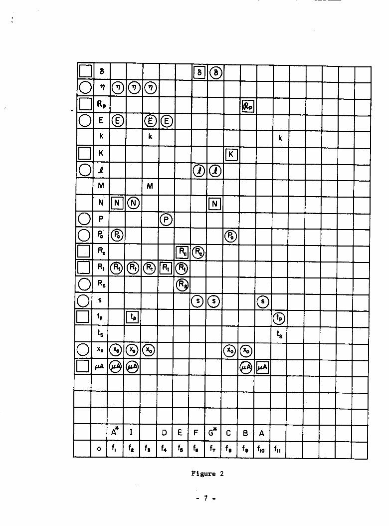
LJ 8

0 ",@@ @I I _.,

0_@ @@k

UiK

OJ

k

M

®®

0

®®M

N

OP0_®

0 _, @O_ ®®

ts

_o®®®

INI

®

®

®

®

0

A_ ! D E F G_ C B A

fa f2 f_ f4 f5 fs f7 fe f_ fao fl I

Figure 2

-7 -

Any relay uhich satisfies these three require_en! s is an acceptable

design_ T]is set is referred to as the primary set of specifications. There

also exists a seconda_ _ set of sfecifications chosen by the designer as

uentioned e:_rlier. In other *._ords, if the primary specifications do not com-

fletely (_etermine N-V parameters of the relay design matrix, the designer then

selects some additional desi_n m_trix parameters at his discretion, ?.,!anytimeseconomic factors influence this selection.

The design process, as explained earlier, requires that the specifica-

tions for the device be stated in terms of kn_<n parameters. Comparing the

specifications listed above with the parameters listed on the design matrix

it is easily seen that there is a gap between the specifications and the

beginning of the logical design process. This gap may be filled by another

design, say a contact design matrix, relating the parameters determined by the

primary specifications to the parameters in the actuator design matrix.

From the contact design matrix the primary specifications applicable to the

actuator design matrix are determined. Investigation of a suitable contact

design matrix is under development at the present time.

Ideally, all significant parameters of a relay system could be listed on

a design matrix, allo_cing the engineer to proceed in a logical manner,

directly from the specifications to the final design. In other words, the

present design matrix is sub-matrix of a larger, more complete relay designmatrix.

As an example of this overall procedure, consider the set of specifica-

tions listed above. The first condition is related to shock. The second

condition refers to the design of the contacts (switching capacity.) Assume

that a contact design matrix is used to obtain a set of contacts satisfying

this requirement. The parameters specified by this contact design matrix

would be Xo, Po and M.

Considering the third condition, the parameters specified are _ and s.

These plus the parameters specified by conditions I and 2 specify Po, xo, M,

£, and s. Since it is possible to fix eight parameters and obtain a design

with this design matrix, the designer now has an opportunity to select three

other Farameters of his choice.

The choices are 6, (in order to use standard size wire), _ (for good

stability), and Rs (the external series resistance.) Combining the primary

specifications and the chosen parameter, the parameters _, 6, R s, £, s, Xo,

M, and Po are fixed. Inherent restrictions are on _, _, g', a and _.

In order to illustrate the result of selecting a set of parameters which

are not usually selected, the following example using numerical values is

siven.

: .5 ,, Po = 70 gm B = .4

6 = 5 x I0 "3 xo = 20 x I0 "3'' _ = .I

P, = l" M = 8 gm 6' = .47

s = .75" Rs = 0 a = 1

O' : X 0

Applying the set of parameters _, 6, R s, £, s, Xo, M and Po to the actuatordesign matrix, shown in Figure 3 shows that a general solution exists. The

-8-

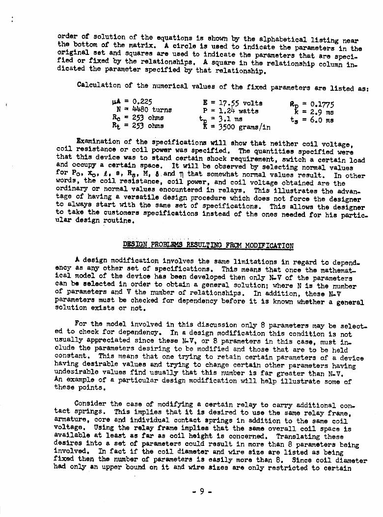
order of solution of the equations is shown by the alphabetical listing nearthe bottom of the matrix. A circle is used to indicate the parameters in the

original set and squares are used to indicate the parameters that are speci-fied or fixed by the relationships. A square in the relationship column in-

dicated the parameter specified by that relationship.

Calculation of the numerical values of the fixed parameters are listed as:

_,A = 0.225N = /4480 turns

= 253 ohms= 253 ohms

E = 17.55 volts

P = 1.24 watts

= 3.1 ms= 3500 grams/in

o.17752.9 ms

ts = 6.0 ms

Examination of the specifications willshow that neither coil voltage,coil resistance or coil power was specified. The quantities specified were

that this device was to stand certain shock requirement, switch a certain load

and occupy a certain space. It will be observed by selecting normal values

for Po, xo, _, s, Rs, M, 8 and _ that somewhat normal values result. In other

words, the coil resistance, coil power, and coil voltage obtained are the

ordinary or normal values encountered in relays. This illustrates the advan.

rage of having a versatile design procedure which does not force the designer

to always start with the same set of specifications. This allows the designer

to take the customers specifications instead of the ones needed for his partic.ular design routine.

DZSlSN PROSLmS P SUL n UFROM MOD ICATION

A design modification involves the same limitations in regard to depend.ency as any other set of specifications. This means that once the mathemat.

ical model of the device has been developed then only N-V of the parameterscan be selected in order to obtain a general solution| where N is the number

of parameters and V the number of relationships. In addition, these N-V

parameters must be checked for dependency before it is known whether a generalsolution exists or not.

For the model involved in this discussion only 8 parameters may be select-ed to check for dependency. In a design modification this condition is not

usually appreciated since these N-V, or 8 parameters in this case, must in-

clude the parameters desiring to be modified and those that are to be held

constant. This means that one trying to retain certain parameters of a device

having desirable values and trying to change certain other parameters having

undesirable values find usually that this number is far greater than N-V.An example of a particular design modification will help illustrate some ofthese points.

Consider the case of modifying a certain relay to carry additional con-

tact springs. This implies that it is desired to use the same relay frame,armature, core and individual contact springs in addition to the same coil

voltage. Using the relay frame implies that the same overall coil space is

available atleast as far as coil height is concerned. Translating these

desires into a set of parameters could result in more than 8 parameters being

involved. In fact if the coil diameter and wire size are listed as beingfixed then the number of parameters is easily more than 8. Since coil diameter

had only an upper bound on it and wire sizes are only restricted to certain

-9-

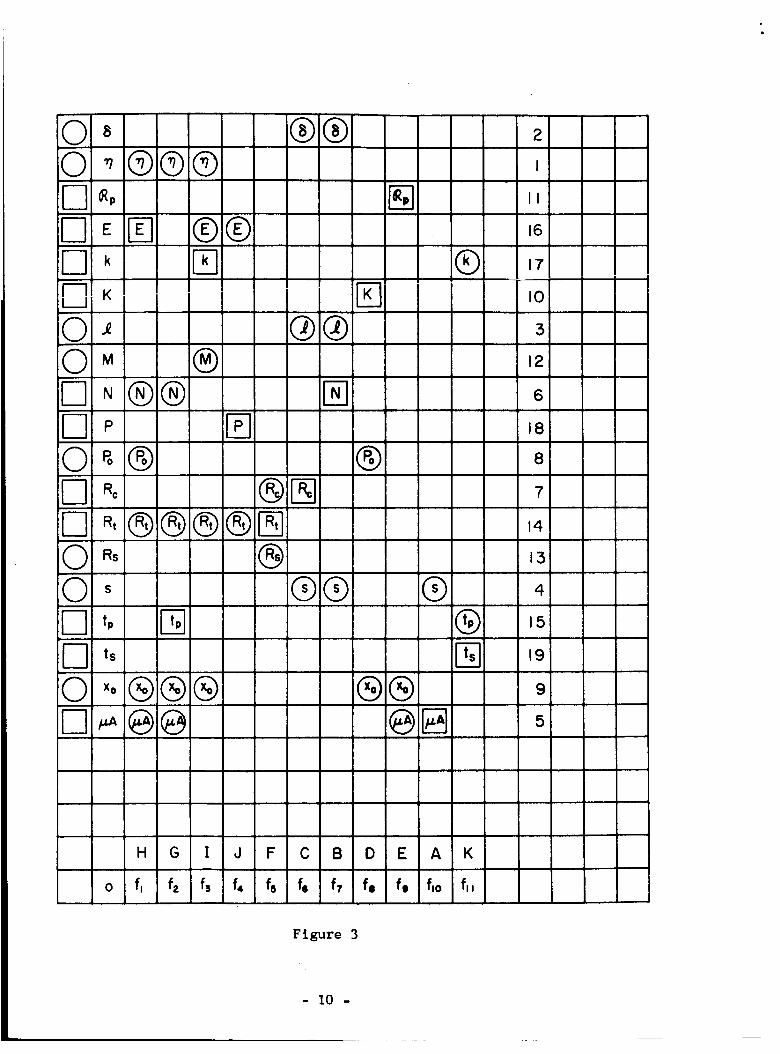
00E][3[3F-I00[3[30[3[300E][30[3

8

_p

E

k

K

M

N

P

g

IRc

Rt

Rs

$

t.

ts

Xo

@

M

@

@

®

®®

®

®

®

D

(9@

®

@I-q

®

®

®

®

IZl

®®

®

®

@

®

®

®

®

(9

i-q

®

®

®

6)

2

I

II

16

17

I0

3

12

6

18

8

7

14

13

4

15

19

9

5

0

H G I J F C

f, f2 f3 f4 f5 f,

I

B

f7

Figure 3

- 10 -

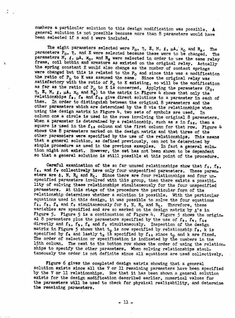
numbers a particular solution to this design modification was possible. A

general solution is not possible because more than 8 parameters would havebeen selected if s and 8 were included.

The eight parameters selected were Po, _, E, M, _, aA, xo and Rs. The

parameters Po, _, and E were selected because these were to be changed. The

parameters M, _, _A, xo, and Rs were selected in order to use the same relay

frame, coil bobbin and armature as existed on the original relay. Actually

the spring constant K would also change as the number of contact springs

were changed but this is related to the Po and since this was a modification

the ratio of Po to K was assumed the same. Since the original relay wassatisfactory with the ratio of Po to K existing, so will be the modification

as far as the ratio of Po to K is concerned. Applying the parameters (Po,_, E, M, _, _A, xo and Rs) to the matrix in Figure 4 shows that only the

relationships fs, f¢ and f:0 give direct solutions to a parameter in each of

them. In order to distinguish between the original 8 parameters and the

other parameters which are determined by the 8 via the relationships when

using the design matrix in Figure 4, two sets of symbols are used. In

column one a circle is used in the rows involving the original 8 parameters.When a parameter is determined by a relationship, such as s in fle, then a

square is used in the f10 column and the first column for that row. Figure 4shows the 8 parameters marked on the design matrix and that three of the

other parameters were specified by the use of the relationships. This means

that a general solution, as defined previously, can not be determined by

simple procedure as used in the previous examples. In fact a general solu-

tion might not exist. However, the set has not been shown to be dependent

so that a general solution is still possible at this point of the procedure.

Careful examination of the so far unused relationships show that fl, fs,f6, and f_ collectively have only four unspecified parameters. These param-

eters are _, N, Rc and Rt. Since there are four relationships and four un-

specified parameters involved with this group, then there exists a possibi-

lity of solving these relationships simultaneously for the four unspecified

parameters. At this stage of the procedure the particular form of the

relationship determines whether a solution is possible. With the particular

equations used in this design, it was possible to solve the four equations

fl, fs, f6 and f7 simultaneously for 8, N, Rc and Rt. Therefore, these

variables are specified and are so marked on the design matrix by A's in

Figure 5. Figure 5 is a continuation of Figure 4. Figure 5 shows the origin-

al 8 parameters plus the parameters specified by the use of fe, fe, flo

directly and f:, fs, f6 and fT simultaneously. Inspection of the design

matrix in Figure 5 shows that tw is now specified by relationship fz, k is

specified by f4 and lastly ts i_ specified by f11 since tp and k are fixed.The order of selection or specification is indicated by the numbers in the

15th column. The next to the bottom row shows the order of using the relation.

ships to specify the other parameters. When solving relationships simul-

taneously the order is not definite since all equations are used collectively.

Figure 6 gives the completed design matrix showing that a general

solution exists since all the V or II remaining parameters have been specified

by the V or II relationships. Now that it has been shown a general solution

exists for the design modification described earlier, numerical values for

the parameters will be used to check for physical realizability, and determinethe remaining parameters.

- II-

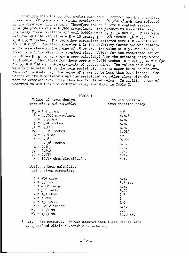
Starting _ith the contact system each form C contact set has a contactpressure of 68 grams and a spring constant of 2287 grams/inch when referredto the armature pull center. Therefore for an 8 form C contact systemPo = 544 grams and K = 180300 grams/inch. The parameters associated withthe relay frame, armature and coil bobbin were M, _, _A and xo. Theseweremeasured and the values were M = I0 grams, _ = 0.94 inches, _A = .582 andxo = 0.017 inches. The two other parameters selected were E = 24 volts dcand h = 0.56. The last parameter h is the stability factor and was select-ed as some,wherein the range of .5 or so. The value of 0.56 was used inorder to utilize wire of a standard size. Values for the restricted set ofvariables B, P, _, c, a and g were calculated from the existing relay whereapplicable. The values for these were _ = 0.036 inches, a = 2,105, gr = 0.692and gn = 0.639 and _ = resistivity of copper wire. The values of 8 andwere not selected since the main restr_ction was an upper bound on the out-side coil diameter s. The value of s was to be less than 0.75 inches. Thevalues of the 8 parameters and the restricted variables along with theresults obtained from using them are tabulated below. In addition a set ofmeasuredvalues from the modified relay are sho_ in Table I.

Values of given designparameters and variables

TABLEIValues obtained

from modified relay

Po = 544 grams 503K = 18,300 grams/inch n.m._M = l0 grams n.m.

= 0.94 inches n.m._A = 0.582 n.m.xo = 0.017 inches 0.015E = 24 v dc 24h : 0.56 0.602

= 0.036 inches n.m.a = 2.105 n.m.

gr = 0.692 n.m.gn = 0.639 n.m.

p = 10.37 ohms/cir.mil.-ft, n.m.

Design values calculatedusing given parameters

6 = #34 wire n.m.k = 5.2 ms. 3.5 ms.N = 4080 turns n.m.P = 3.8 watts 3.97

Rc = 151 ohms 1_5Rs = 1 ohm 1Rt = 152 ohms 146

s = 0.712 inches n.m.tp = 10.1 ms. 8.3t s = 15.3 ms. ll.8 ms.

n.m. = not measured. It was assumedthat these values wereas specified within reasonable tolerances.

- 12-

A comparison of the design values with the measuredvalues show somedifferences. These are to be expected since certain tolerances must existon the physical device. In the case of Po it was assumedall the contactsinvolved in a form C set were the same. The results show about a 6%difference. Since K was not measuredon the modified relay it was assumedthat it was as assumed. The air gap x_ was not set exactly at the designvalue giving about a 10%difference. The stability factors were about 10%different. The transit times differed about 30%which could be caused bythe deviations noted above. However, the assumptions used in developingthe design equation for k were such that the design value should normallybe larger than actual values, which is the case here.

The measuredpower P is a little high caused by the coil resitance Rcbeing lower than the design value. The plck-up times differed by about20% which could be caused by the differences in Po and xo and other toler-

ances. Again the design value is larger so that the actual seating time tsis less than the design value. These noteddeviations explain why a stabil-

ity factor of about 0.5 is necessary. These deviations included with the

regulation of the power supply and the increase in ambient temperature all

go toward the determination of the stability factor h.

This section of the paper indicates some of the problems that exist

in a relay design modification. The important point is that a limited

number, namely N-V, of the design parameters can be selected. These N-V

parameters must include those that are to be changed and those that are to

be maintained the same. The other or V parameters must be allowed to vary

in order to satisfy the requirements on the N-V parameters.

CONCLUSIONS

It is seen that the number of items which maybe specified is fixed

with a given number of parameters and relationships. Many abitrary specifi-

cations have been shown to be impossible. This has been accomplished by a

logical procedure. Conflicting specifications may not be evident until the

items have been checked by the logical procedure.

Before a design may be started it is necessary to formulate the relation-

ships with the parameters which are involved in the device to be designed.

The design theory presented is that of organization. The ideas used

are those of "system coherence" and "set independance." A simple system

matrix is constructed by using sets of elements from physical laws and

arbitrary restrictions. From the system representation and some given

specifications an orderly technique is used to determine if these specifi-cations can be satisfied. The distinct difference between the numerical

problems of a solution, inevitable in an actual design, from the generalsolution which indicates how to solve the numerical problems are illustrated

by specific examples. It is the relation between the general solution of a

system and a particular solution which can be used to increase the efficiency

of solving design problems.

REFERENCE

* "Theory of Design", C. F. Cameron, D. D. Lingelbach & C. C. Freeny; NinthNational Conference on Electromagnetic Relays, 1961.

-13-

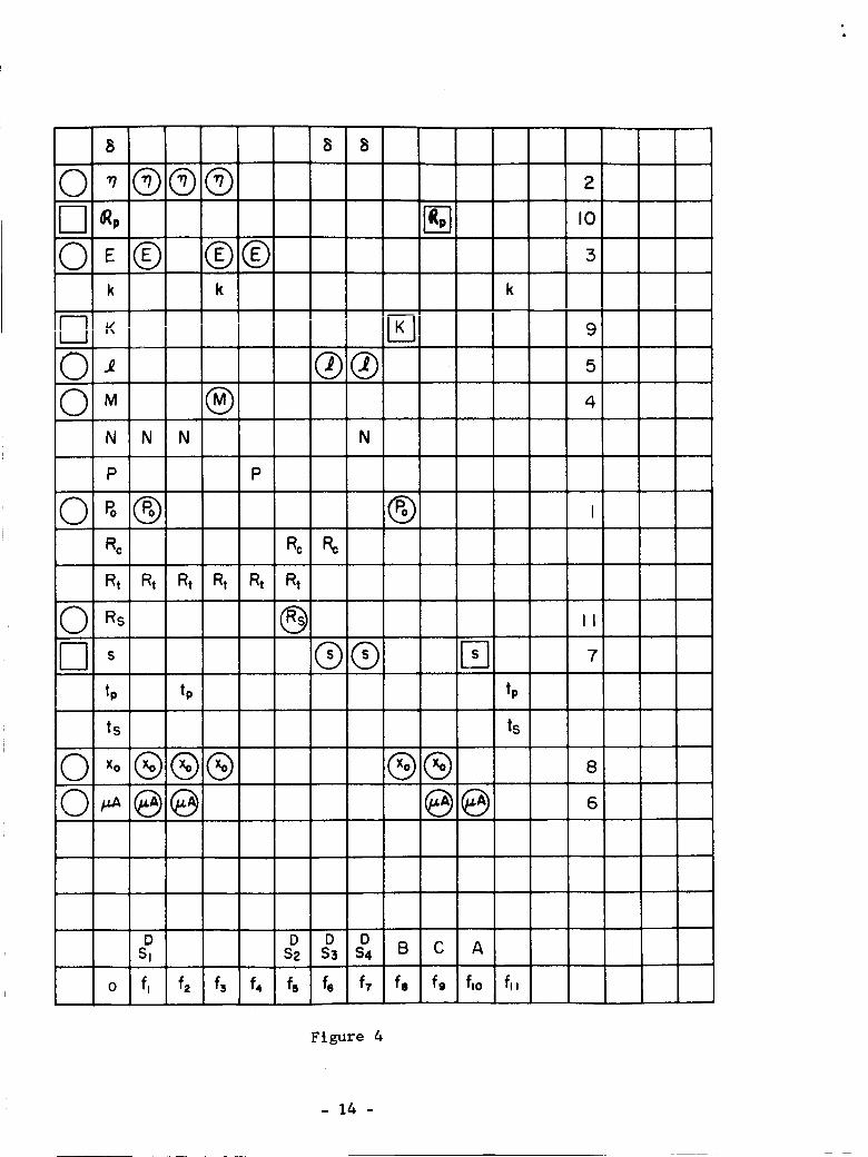
8

0_@@@I-1 _,

Q_®k

®®k

K

O_0 M

N

®N N

P

0_@Rc

Rt Rt

D_tp

P

Rt Rt Rt

tp

ts

0 xo@®®0_®@

%

Rt

®

8 8

®®

N

%

®®

F6

®

½

®®®®

tp

ts

2

I0

3

9

5

4

II

7

8

6

DSi

D D D$2 $3 $4 m

o f, f, f3 f4 f5 f6 f7 fa

C A

f9 f,o fll

Figure &

- l& -

_®®®l--i s,OE® ®®

k k

IZIKii

0-' ®®®M

A_®®P

0_®£_ , ®®A _'®®®i®®

r-I_tp

P

®

®®tp

0 'o®®®

F_

®

E]

®®@@

tp

ts

12

2

I0

3

9

5

4

13

I

14

15

II

7

8

6

D D DSz S3 S4 B C A

o fl fa fl f4 f8 fl f7 fe fl flo f,I

Figure 5

- 15 -

A'_ @®0 ' @®@

0_@ @®-1 _ IEi

0-_ ®®0 _ ®A_@@ ®liP i0_@A _o ®:@A ', ®®®®®

---- tp

--1 tso 'o®®®0_@@

'®

$

®®®@

®

®t_2.s

12

2

I0

3

17

9

5

4

13

18

I

14

15

II

7

16

19

8

6

D D DS_ E F G Sz S3

o f, f2 f_ f4 fs f6

Ds4 B

f7 fe

Figure 6

- 16 -

SECTION I

PRELIMINARY CONTACTOR REDESIGN

Preliminary vibration testing of four contactors with ratings from 254

amperes to 200 amperes show that the plunger is moving when the coll is de-

energized. The motion of the plunger occurs at different G levels for the

different contacto_a However, thlsG level is below the specified 20 g.

For the de-energlzed case the plunger showed motion before contact chatter

was indicated. This suggests that the plunger motion influences the contact

chatter in the de-energlzed case. Any change in the design to stop the

plunger motion will influence the other characteristics of the contactor,

therefore a preliminary redesign should be made to determine some idea of

the changes involved.

To stop the plunger motion when the contactor is being vibrated at 20 g

with the coil de-energlzed requires that the initial back tension on the

plunger be at least 20 times the mass of the moving parts. Since an opened

200 A contactor was supplied, it will be used to demonstrate the redesign

procedure. The redesign for the other contactors would be essentially the

same but _th different numerical values.

For the opened 200 A contactor provided, the total mass of the moving

part is 85 grams. Since this is to withstand 20 (_) g peak, this member

must be preloaded mechanically against the back stop with a force of at least

29 x 85 or 2460 grams. The initial back tension existing on the contactor

presently is about 1200 grams. A mathematical model of a contactor will be

used to determine the overall change in the characteristics when the back

tension is increased. The mathematical model being used allows only 8

parameters to be changed or held fixed. Some parameters are easier to change

than others because this is a redesign and changing the mechanical quantities

may be more difficult than changing electrical quantities. '_ith this in mind

I- I

the following paramteres are selected to be held fixed: E, _, s, M, Xo, _A,

_. The parameter being changed is Po, the back tension. This set then in-

cludes 8 parameters which are all that can be specified, in general. Before

checking for dependenceyof the parameters, the reasoning behind selecting

these, is in order at this point. The supply voltage E was selected as one

parameter since the contactor apgllcation was to be the same. The parameters

and s were selected since these represent the coll dimensions and if

possible it is desirable to use the sameenclosure. The mass of the moving

parts is to be unchangedif possible at this point so the parameter M was

selected. No changewas to be madein the magnetic circuit so xo and _A

were selected. The overall operating stability was to be the sameor improved

so _ was selected as one parameter. Table I gives a list of the symbols and

their definitions.

To check to see if the parameters are independent as far as the mathe-

matical model is concerned, the design matrix given in Figure 1 is used.

This design matrix gives the parameters as row positions and the relation-

ships relating these parameters as column positions numberedfl to f,1 in-

clusive. Table II gives the mathematical form of each relationship f,

through f1_. To use the design matrix shownin Figure l, each parameter of

the 8 selected is indicated with a circle in column one at the row corres-

ponding to the parameter. This procedure is shown in Figure 2. After or

during the marking of the 8 parameters, each relationship (column) is check-

ed to see if all of the parameters in that relationship are circled (selected).

If all the parameters in any relationship are circled (selected), then all

of the parameters in that relationship are not independent. This meansthat

if the relationship contains m parameters, only m-1 can be independent. In

other words this meansthat any m-1 parameters of an m parameter relationship

determines the remaining parameter by the use of that relationship.

2- I

TAHLEI

Parameter Symbols and Definitions

Map parameters


¶ = design stability point

_p = reluctance of magnetic circuit presented to the coil with theplunger.in the pick-up position

E = open circuit supply voltage

k = armature transit or travel time

E = effective spring constant of spring system

= coil length

M = effective plunger mass

N = coil turns

P = steady state total po_r supplied to relay coll circuit by source E

Po = back tension at plck-up


Rt = total resistance of relay coil circuit presented to voltage source E

Rs = Rt - Rc

s = outside coil diameter

tp = armature pick-up time

ts = armature seating time and equals tp + k

_A = permeability of free space times the effective cross sectional area

of the working air gap

xo = plunger working air gap

Restricted parameters

B = ratio of core diameter to outside coil diameter

_i = magnetic reluctance of the non-working magnetic circuit

p = resistivity of conductor material

= air equivalent of the non-working part of magnetic circuit when

using a series representation

J 3-1

= ratio of twice the coil bobbin wall thickness to the outside coildiameter

gr = resistance winding space factor

gn = turns winding space factor

a = ratio of pole face diameter (d') to the core diameter (d)

u = twice the thickness of the coil bobbin

d - core diameter

TABLE II

Mathematical Form of Relationships in Mixed Units

Units involved are:

mass (M) in grams

force (Po) in grams (gram gage measures force in grams)

length in inches

voltage in volts

current in amperes

resistance in ohms

permeability of free space (_) is 3.19 lines/amp-turn inch

magnetic f_u( in lines

magnetomotive force in ampere-turns

power in watts

time in seconds

magnetic reluctance (Rp) in amp-turns/line

Relationships:

(f,) _ - (157.5)Rt(Xo + _ PoENq-_ -0

(f,)

(fs)

Nz ,LA I

tp- (10-s) (Xo+_)Rt _n _ = 0

1k - (8.66 x 10 -3 ) 18 M Xo z Rt =0

(1-_)[I- V'(l_o° )

4- I

(f*) P- ]_'I_o = o

(s,) _ - (Rs+ Re) = o

(f6) Rc . (0.865 x l0-6) _rs z (l_- 8 - a)(1 + 8 + _) t8"

(f_) __ o.6_7 _n (_ - _ - _) _s8

2 Po(fa) K -

xo*-"_ < o

(f,) Rp - x°+_-_--0

(f:o) _A. tta'sZ_z_" 4 = 0 (_ =3.19)

(it:) ts - (tp + k) = 0

Auxiliary relations

_7= -a--oeVxo

I_ = d/s

= U/S

a = d'/d

=0

Examination of Figure 2 shows that in relationship fle, all the param-

eters are selected (circled). This means that in general both s and _A can

not be selected, i.e., one determines the other. Since only one of these

(s or _A) can be selected, then another parameter must be selected. The

parameter Rs, which is the resistance in the supply, will be selected instead

of s, since the application of the contactor is fixed. The 8 parameters now

are: E, L, M, Xo, _A, _, Rs & Po. Using these 8 parameters, the design

matrix in Figure 3 is obtained with circles u_ed to indicate the original 8

selected parameters. Examination of the design matrix shows that relation.

ships fe, f_ and it0 have all but one parameter selected. A square is used

5- I

to indicate that a parameter has been determined by the use of one of the

relationships. After marking these newly determined parameters the design

matrix shown in Figure 4 is obtained. Examination of this Figure _ shows

no relationship having all but one parameters marked. This might suggest

that another parameter needs to be selected but if this is tried, a conflict

will exist where two relationships will determine the same parameter.

Closer examination of the design matrix in Figure $ will reveal that their

are four relationships involving four unselected (un-marked) parameters.

These four relationships are f:, fs, f6 and f7 and the parameters are N,

Rt, R c and 6. Four equations and four unknowns suggest simultaneous

solution of the equations to obtain a solution. At this point in the design

the mathematical form of the equations must be used. Up to this point, only

the variables or paramters involved were used. Relationship fl could be

solved for N or Rt, fs for Rt or Rc, f6 for R c or 8 and f7 for N or 6.

Solving f5 for Rc and substituting into f6 eliminates R c. Then substituting

for R t in f: by using f6 gives two equations involving N and 6. These

equations are:

N- .637 gn (1-B-a) s_

6 (I)

= ,865xi0"6Tgr (xo+ 2krf 8" E _ _A (2)

Solving these two equations for 62 gives:

_, = .865 x 10 -6 gr (3+8+_) s (Xo+_)%_ Po

.637E (3)

This shows that the parameters N, Rt, R c and 8 are determined by those

already marked in Figure _. These parameters are marked as shown by the

design matrix in Figure 5 and the other relationships fz, f$, f4 and f11

have all but one parameter selected (marked). The result shown in Figure 5

means that in general the 8 parameters E, _, M, Xo, _A, _, R s and Po can be

6- I

used to determine the other II parameters. Figure 5 also shows the order

in _hich the relationships are to be solved and the particular parameter

solved for. This is indicated by the alphabetical letterin_ on the bottom

row. The order in which the parameters are used is shovm by the numerical

sequence in the column at the right.

Only one parameter of the original _ is being changed, the others are

held fixed. At the present time no dra_in% or information is available

about the coil size and magnetic circuit so the redesign _,ill be done in

terms of the percent change in the parameters. In other words, the ne_

values _ill be ziven in terms of the old values as a percent change. The

design matrix indicates that f10 is the first relationship used. This

relationship is used to solve for s. Since _A was to he unchanged so v_il]

s be unchanged since a and B are fixed.

Relationship f, indicates that the parameter ep is unchanged since Xo,

_A and _ are unchanged. From f8 the value E must be less than 2 Po/(Xc_ + _)

and since Po is the only one changed and it is increased then using the same

springs as on the original _i_l still satisfy f8 so E can remain unchanged!.

Equation 3 developed in this discussion is used to determine the ne_

value of 6z. The term gr is the resistance ,_inding factor and may be assumed

essentially constant for small changes in wire size. All the other parameters

except Po are constant therefore the ne_ value of 62, say 6:z, _dll be:

6J= 1.43_- q ]2OO =

Therefore the ne_ circular rail size of the _ire should be 43_ larg_" than th_

old or 81a = 1.43 8z. Equation 3 was the result of solvin_ four equations

simultaneously, therefore, the other 3 parameters involved must be solved for

next, The parameter N (coil turns) can be solved for by using fv, _,_hichwas

one of the 4 relationships used for simultaneous solution. Examination of f7

7- I

shows that all the parameters are constant except 6z (wire size). Since the

new value of wire size is 1.43 times the original then the new N (or N,) will

be given as

N,= 1N 1.4---3or N, = .70 N (5)

This means the new number of turns will be 70_ of the original number of turns.

The next parameter involved in the simultaneous solution is Rc. Relation-

....... _4 hasship f6 is used to determine Rc. Relationship f_ shows %ha+ _ly

changed in this case. Therefore the coll resistance is given as:

1Rc _ = .487 or Rc, = .487 Rc (6)

This gives the new total resistance as 48.7% of the original total resistance.

The value of R s is the same but the total resistance Rt will decrease because

Rt = Rs + Rc and Rc is 48.7% of its original value. The total resistance Rt

is the last parameter of those solved simultaneously. Figure 5 indicated that

tp is the next parameter solved for and it is obtained by relationship fz.

This relationship involves two parameters which have been changed._ •These are

N and Rt. Using the relationship fz gives the new value of pick-up time (tpl) in

terms of the original as: tp: - IO'8_('70N)*S _A £n 1(Xo + _)[.487RtS _ (7)

(.70)ztp, = ._87 tp = tp. (8)

The result shown by equation 8 means that the new pick-up time (tp,) is the

same as the original pick-up time.

The transit time k is the next parameter calculated and this is accomp-

lished by using relationship f3. Inspection of relationship f3 shows only

two of the parameters are changed. These two are Rt and Po- The manner in

which Po changes k is not a direct variation because the operations involved

are sum and differences. Past experiments have indicated that the influence

of Po on k is normally not great. Also since the numerical value of _ has

8- I

not been determined, it is desirable to not consider the effect of Po in

this particular relationship.

will be given as

Therefore the new value of transit time (k,)

k, = '$.487 k,= .785 k. (9)

This gives the new value of transit time (kl) as 78.5% of the original value.

The coil power is computed next using relationship f,. Since Rt is the

only parameter changed, then the new value of coil power (PI) is:

l P= 2.05 P if Rs 0 (lO)P* = .48---_ =

The new coll power is 105% larger than the original. With this increase in

coil power, a re-evaluation of the thermo-dissipation may be necessary.

Design equations for the heat dissipation have not as yet been developed.

The last parameter calculated is the total seating time ts. The relation-

ship used is f** and since its form is the sum of tp and k, only the relative

change can be given. Since the new value of the plck-up time is the same as

the original and since the new transit time is less than the original, then

the total seating time (ts,) will be less than the original. Table III gives

a summary of the results of a new design calculation in terms of the original

values. Percentage changes have been given when possible and relative changes

for the other cases.

TABLE III

Comparison of the new values of the contactor parameters in terms of the

original values when E, _, M, xo, _A, _, Rs are fixed and Po increased.

Design parameters

8z = area of bare wire

= design stability point

ep = reluctance of the magnetic circuitpresented to the coil with the

plunger in the pick-up position

E = open circuit supply voltage (dc)

43% larger

specified same

no change

specified same

9-I

k = plunger transit time

K = effective spring constant of

spring system

= coil length


N = coil turns

P = total steady state power to

contactor from voltage supply

Po = effective back tension at pick-up


R t = total resistance of contactor

circuit presented to voltage supply

R s = Rt - R c


tp = plunger pick-up time

t s = plunger seating ti_e

Xo = plunger _rking air gap

_A = permeability of free space timeseffective cross sectional area of

working air gap

21.5% smaller

no change needed but maybe

increased 100% if necessary

to obtain desired Po

specified same

specified same

30% smaller

105% larger

specified 105% larger

51.3% smaller

51.3% smaller if Rs = 0

specified same

no change

no change

less

specified same

specified same


B = ratio of core diameter to out-side coil diameter


= air equivalent of non-working part

of magnetic circuit when using a

series representation

= ratio of twice the coil bobbin wall

thickness to the outside coil diameter



a = ratio of pole face diameter (d')

to the core diameter (d).

I0- I

assumed constant

assumed constant

assumed constant

assumed constant

assumed constant

assumed constant

assumed constant

A study of Table III may suggest that the parameters that were selected

be held fixed, are not the most desirable. Particularly since the coil power

required has more than doubled, it might be desirable to consider holding the

coil power constant and letting the coil height vary instead. With this

change the second set of selected parameters would be _, E, M, P, Po, Rs, Xo

and _A. Figure 6 shows the parameters marked on the design matrix. The

results show that f6 and f7 must be solved simultaneously for _ and 6. Solu-

tio_ of these two equations gives

6z 0.865 x 10-6 _rS(l ÷ B + _)N (Ii)= .637 gn Rc

The solution order is given in Figure 6 showing that f:0 is used first

to solve for s. Since _A is constant then the new value of s(given as s,)

is the same as the original. Therefore, sz = s. Relationship fe iodicates

that K can be unchanged but maybe increased 10S if necessary to get the new

value of Po. The magnetic reluctance ep as given by f, is unchanged since

xO and _A are constant. The value of Rt is unchanged because E and P are

constant. The value of Rc is the same since Rt and Rs are constant. Relation-

ship f, indicates that N will change since Po is changed. The new value Nz

of the number turns is given as

N, = i_0 N = I.#3N. (12)

This means the number of turns required is 43% greater than the original

number.

The new value of tp is given by f, and varies as the square of N.

Therefore, the new value tpz of the plck-up time is

tp, = (1.43) ztp = 2.05 tp. (13)

This means that the pick-up time is essentially doubled. Relationship f3

indicates tha$ k is unchanged since Rt and the other specified parameters are

unchanged.

ll- I

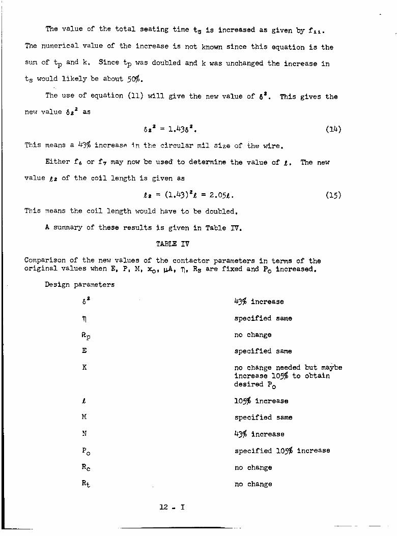
The value of the total seating time t s is increased as given by f**.

The numerical value of the increase is not known since this equation is the

sumof tp and k. Since tp was doubled and k was unchanged the increase in

ts would likely be about 50%.

The use of equation (ll) will give the new value of 8z. This gives the

new value 6z2 as

6,* = 1.4382. (14)

This meansa 43%increas_ in the circular mil size of the wire.

Either f6 or f7 may now be used to determine the value of 2. The new

value _z of the coil length is given as

= = 2.o5 . (15)

This means the coil length would have to be doubled.

A summary of these results is given in Table IV.

TABLE IV

Comparison of the new values of the contactor parameters in terms of the

original values when E, P, M, Xo, _A, _, Rs are fixed and Po increased.

Design parameters

6_

_p

E

K

M

N

Po

Rc

Rt

43% increase

specified same

no change

specified same

no change needed but maybe

increase 105% to obtain

desired Po

105% increase

specified same

43% increase

specified 105% increase

no change

no change

12- I

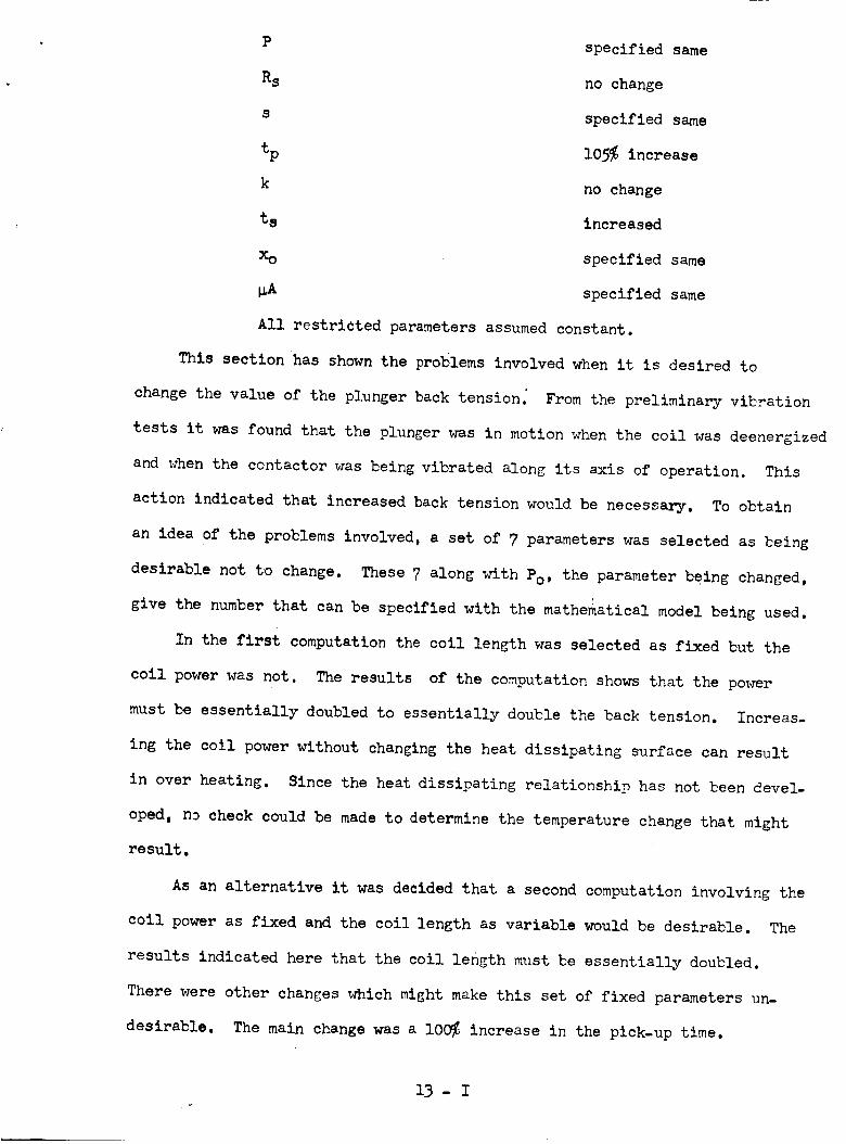
P specified same

Rs no change

s specified same

tp 105%increase

k no change

t s increased

xo specified same

_A specified same

All restricted parameters assumedconstant.

This sectionhas shownthe problems involved when it is desired to

change the value of the plunger back tensionj From the preliminary vibration

tests it was found that the plunger was in motion when the coil was deenergized

and whenthe contactor was being vibrated along its axis of operation. This

action indicated that increased back tension would be necessary. To obtain

an idea of the problems involved, a set of 7 parameters was selected as being

desirable not to change. These 7 along with Po, the parameter being changed,

give the number that can be specified with the mathematical model being used.

In the first computation the coil length was selected as fixed but the

coil power was not. The results of the computation shows that the power

must be essentially doubled to essentially double the back tension. Increas-

ing the coil power without changing the heat dissipating surface can result

in overheating. Since the heat dissipating relationship has not been devel-

oped, no check could be madeto determine the temperature change that might

result.

As an alternative it was decided that a second computation involving the

coil power as fixed and the coil length as variable would be desirable. The

results indicated here that the coil length must be essentially doubled.

There were other changes which might make this set of fixed parameters un-

desirable. The main changewas a 100%increase in the pick-up time.

13-I

Whether this is critical or not depends on the application.

These two sample computations should point out the basic restrictions

involved in a redesign and that is:only a limited number of parameters can

be fixed or changed. A realization of this restriction usually means that

a critical evaluation must be made of the parameters that must be fixed.

increase in the required back tension usually means an increase in coll

power or an increase in coil volume or a combination of both.

An

14- I

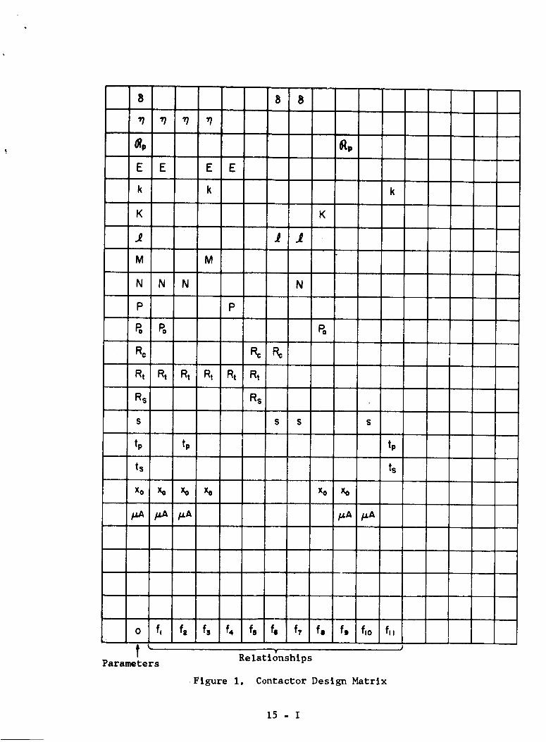
8

E E E E

k k

K

M M

N N N

P P

Ro P,=

Rt RI Rt Rt Rt Rt

Rs Rs

S

tp tp

ts

xo x= xo xo

8 8

J J

N

_p

K

Po

S S S

Xo xo

p.A /u.A

tp

ts

o f,

t'Parameters

f= fs f4 f8 f6 f7 f, f, f,o f,,

Relat !onsh!ps

•Figure I. Contactor Design HatrIx

15 - I

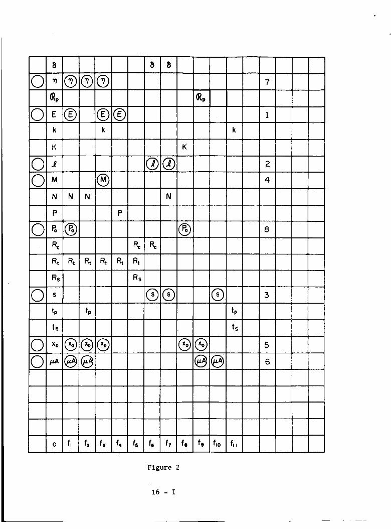
8

0_@@@_p

0_@ @@k k

,v

©_0 _ ®

N N N

p P.

©_®%

Rt Rt Rt Rt Rt

Rs

©_tp tp

ts

xo®®®0_@@

%

Rt

Rs

8 8

®®

N

R=

K

®

®® ®

®®@@

k

tp

ts

7

2

4

8

3

5

6

o fl f= f3 f4 f8 f6 f? fa f9 flo f;j

Figure 2

16 - I

8 _ 8

0_® @®k k

K

OJ ®®O_ ®

N NN N

P

0!_®

Rt Rt

P

Rt Rt

R= R=

Rt Rt

0 R, (_)

_p

K

®

IS S I S S

!

tp tp 1

t s

0 '0®®® ®®0_@@

k

tp

ts

6

2

3

8

7

4

5

o f, f= f= f4 f5 f= fz f= f, f,o fll

Ftsure 3

17 - I

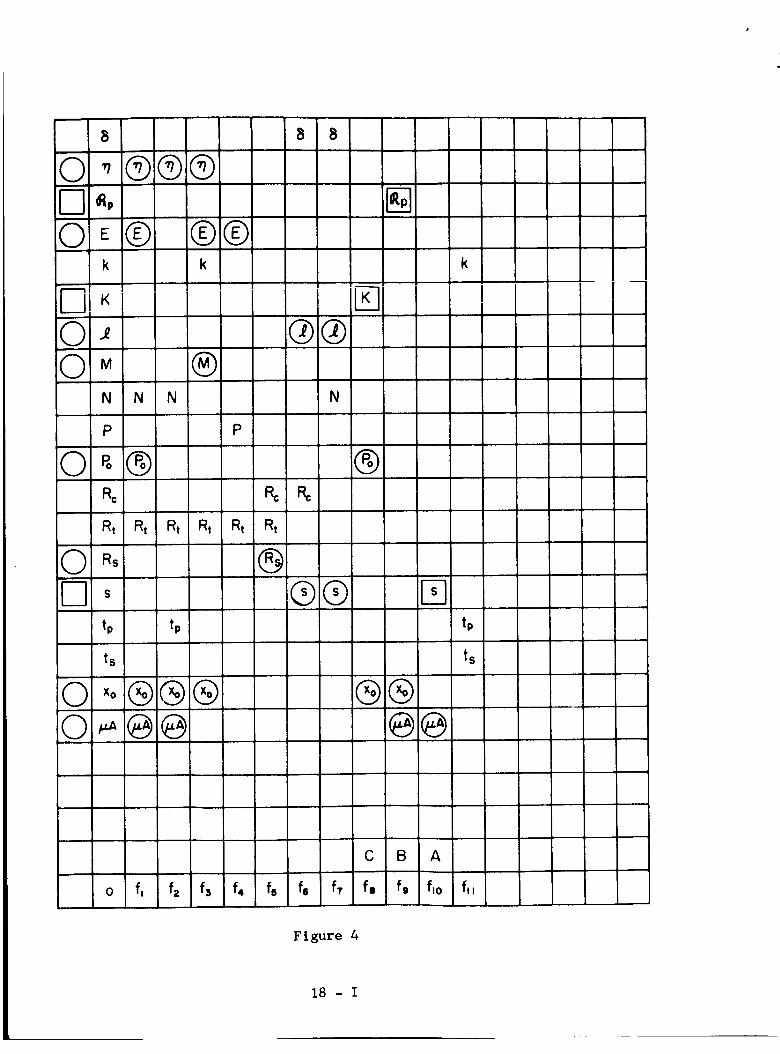
8

0_@®@I-1_,,0_®

-'iI K

O_0 M ®

N N N

P

a®Rc

Rt Rt Rt Rt

Rs

S

tp tp

ts

0

0[i]

O _o®®®O_@@

k

P

Rt

R¢

Rt

@

8 8

®®

N

®®

®

E]

®®@@

k

tp

ts

o f; f2 f3 f4 f5 f6 f7

Figure A

fll

18 - I

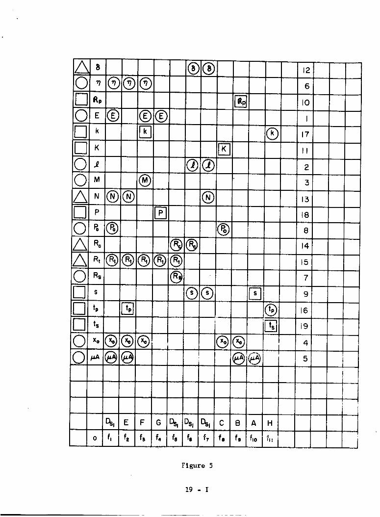
A_ ®®0 _ ,®®®

0_-@ @@11" ± (DLIK I_10'._ ®®,0 _ ®A _ ®® ®__ P L._

.o ®®A _,®®®®®

11 _ ®@ F

L]', " D' [ ®®0 xo®®® , ,

0 _ @:@i I @i @ '

0

Dsj E F G Ds, DsI I_I C B A H

f'If` f' f' f' f' f' f' f' f'°_"i

12

6

I0

I

17

II

2

3

13

18

8

14

15

7

9

16

19

4

5

-q

[

Figure 5

19 - I

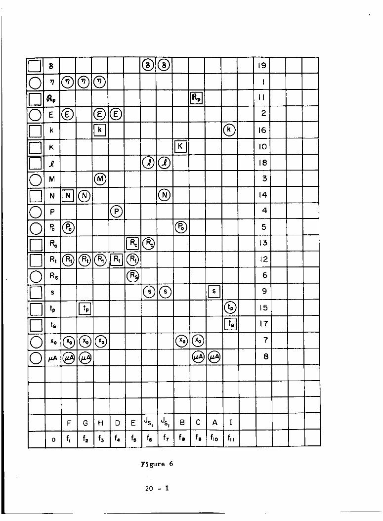
8

0 " @®@r-l _,,OE@I--1,.__1K

0 ,,'r-iN®®OiP

®@EB

®

®O'¢(DMR0 _®I-I R,®i®®_®

71', r-qI-'! t,

0 '0®®®0,_@@

®®

®®

®

@J@ !

@@

®

®U,

19

I

II

2

16

I0

18

3

14

4

5

13

12

6

9

15

17

"7

8

F G H D

fl f= f3 f4

E Js, Js I B C A I

f5 f6 f7 fa f9 flo fll

Figure 6

20 - I

CONTINUATION OF PRELIMINARY CONTACTOR REDESIGN

Report No. 3 Section No. I

Section I of the Interim Report for 1 March to 30 April 1962 was a

discussion of the changes involved in increasing the back tension on the

contactor plunger. The results presented in that discussion were for

two sets of fixed parameters. In one set of parameters, the coil dimen-

sions were held fixed along with six other parameters specified and the

results indicated that the coil power would have to vary directly _th

the back tension. In the other set of parameters, the coil power was

fixed along with the same seven other parameters but the coil length

was allowed to vary. The results in this case indicated that the coil

length varied directly with the back tension. These results are a func-

tion of the particular set of parameters specified.

It now appears that some combination of increased coil power and

coil length might be the most feasible, therefore additional calcula-

tions are given in this section to show the result of increasing the

back tension by a combination of coilpower and coil length. To present

the results in a more enlightening manner the values of the various

parameters are plotted against the coil power. The results are given in

per unit value which is the ratio of the new value to the original value

of the parameter. The original value of the parameter being the value

existing on the contactor furnished by the contractor. To date no

numerical information has been received from the manufacturer of the

contactors furnished but measurements have been made when numerical

values were needed. Fortunately, the form of most of the relationships do

not require absolute values of the parameters. The relative or per unit

value can he used in most of the equations.

The set of parameters specified is; _, E, M, P, P0, Rs, x0 and _A.

I - I

Tab_s I and II given in the previous report are repeated here for conven-

ience of discussion. The value of back tension P0 is to be doubled and

the coil power is increased in increments of 25_ to a total of twice the

original value. The other specified parameters are held fixed at their

original values. Using these parameters on the design matrix gives the

result shown in Figure 1. The order for solvin_ the relationships is

given by the alphabetica] list at the bottom of Fi_,_ I _= _.._--

becomes:

f_0 for s where sz =_a_

fe for K where K <"---='_X 0 +

fe for Rp where Rp = x___A

f, for Rt where Rt = E2/P

f_ for Rc where Rc = Rt-R s

fl for N where N = Rt (xo +q_ (157.5)F--

i_i/__A

lO'_N_ _i_ 1f2 for tp where tp = (xe + _)2_t I---_

f3 for k where k = 8.66 x i0-_ LE,_(I._)[I_( l + Kx@/Po)

fzl for ts where ts = tp + k

f6 and fT for 6 _ere 82 = 0__865 x 10-6_rs(l + 8 +a)N0.637 gn Re

N8 a

f6 and f7 for _ _#r_reZ= 0.637 gn(l-B-_)s

These relationships give the variation in each parameter in terms

of the specified parameters. In this case the two parameters P_ and P

are being increased and _, E, M, Rs, x0 and _A are constant. With these

2- I

conditions the changes that exist for the other parameters are:

s is unchanged,

K varies directly with Pe,

_p is unchanged,

Rt varies inversely with P,

Rc varies inversely with P when Rs = O,

N varies directly with the product Rti2P_o,

tp varies directly with N2 and inversely with Rt,

k varies as the cube root of Rt,

ts varies as the sum of tp and k,

6z varies directly with N and inversely with Rc,

varies directly with the product N6z

The value of P0 was increased to 2 per unit and the value of P was

incremented 0.25 per unit from 1 to 2 per unit. The results of these

changes on the other parameters are given in Table III. The data in

Table III are plotted in Figure 2 with the coil power P as the variable.

These curves show the value of each parameter as the coil power is

changed in order to double the back tension P0. One interesting result

is that the product of coil power P and coil length _ is a constant

having a value of two. Once this result is noted from the curve it can

also be showr_by using the relationships for _, 62 , N, Rc and Rt with

Rs = O,that the product JP is

r0.865 x I0"6_(I + B + _ z_P = 2Po(xo + _)z L (0.637gn)_(1,B._) _ (157.5)

This product _P varies directly with P@ since xo is a fixed para-

meter and all the other variables are restricted parameters. A result

of this kind suggests that a balanced rotary type armature would reduce

this factor of JP since a smaller value of Po could be employed to hold

3- I

_e _rmature open when the coil is deenergized. With the present design

the value of P0 must be such to Gold the total plunger and movabZe con-

tact mass against the acceleration specified. With a balanced rotary

arrangement the value of P0 would be determined primariZy by the opening

contact force required.

Figure 2 also shows that the other parameters either remain con-

stant or decrease as the coil pm_er is increased. The parameters that

w_re __A as being fixed were not sho_n in Figure 2.

Another alternative in modifying a design is to consider making the

coil more efficient. This can be accomplished by changing the ratio of

the iron core diameter to the coil outside diameter. This ratio is one

of the restricted parameters and is designated by the symbol 8. When

the coil bobbin insulation is negligible compared to the coil outside

diameter the value of 8 to make the pull per watt a maximum is 0.6.

Measurements made on the coil of the 200 amp contactor shows that 8 has

a value of 0._35. Therefore, a change in @ should give some impcove-

ment in the coil efficiency° Since 8 _ll now be one of the selected

p_rameters, the design matrix given in Figure 1 _'_

fled to include the parameter 8. Th_s i_ accomolished by exa_l_n< the

relationships to see if they contain _o Those relationships involuting

will now have 8 entered in the column for that relationship. Only three

relationships contain 8 and they are f6, f7 and fla. Figure 3 sho_s the

modified design matrix containing the additional parameter 8. Now the

design matrix contains twenty parameters minus eleven relationships or

nine parameters may be specified. Adding B to the original eight para-

meters will give the nine parameters needed. Figure 3 _hows _ll_ni_e

parameters mapped on the design matrix and gives the order of solution.

The order of solution is as follows:

f_ for Rt where Rt = E2/P

fs for Rc where Re = Rt-Rs

_a zszB _fle for uAwhere _A = 4

fa for K where K < 2P0-x@ @_

f_ for Rp where Rp = xe +__A

fl for N = I_57.5 Rt (xQ + _ 2_Pa

lO'eNZ_A _n 1f2 for tp where tp = (Xo + _) Rt 1-_

F 18 ] */3f3 for k where k = 8.66 x I0"3 LE,_(I_)[I_7,(I + Kxo/P0) ]J

f_ for ts where ts = tp + k

f6 and f7 for 6z where 62 = 0.865 x lO'6_s(l + B + _)_0.637gnac

N_ '

f6 and f7 for _ where _ = 0.637 gn_i-8-_)s .

In these equations the parameter B is involved as a sum -_th the

variable _. Therefore, numerical values of B and a must be used. The

dimensions of the coil result in B = 0.435 and _ = 0.13. The values

used for these calculations are: s = I - 7/16 inch, d = 5/8 inch and

u = 3/16 inch. The value of s is to remain constant so to change

requires that d be changed. The new value of q is to be 0.6 or a change

of 1.38 per unit. This means the factor (1-B-_) changes from O.435 to

0.27 or a 0.62 per unit value. Also the factor (I + 8 + _) changes

from 1.56 to 1.73 or a l.ll per unit value. Using these values and a

value of 2 per unit for P0 gives the results shown in Table IV. The

data shown in Table IV are plotted in Figure 4.

5 - I

Cor,lparison of FicJres_ _J°L:nd '_ ::ho_:s th:t :: v'_-....._ of ;_ of....0,6 _ -

stead of the existing v_lue 0.2535 rom,]ts Jn a decre:_se in the c_i]

length at a given po_:er. Conversely, for a given length, less increase

in coil Do-:or is required to double the back tension. These results

show ths effect of increased col] cfficierc_. In :c_dJt_cn t_ decre::s-

ing the coil len_:th, cth_r decre:::es _Tere Doted _uch as the ',ic]-up

time tp, coil turns I,$and wire size 6_. The coil volume was decreased

because in this case the core diameter was increased while the outside

coil diameter _:as const_nt.

The improvement resulting from increasing 9 from 0.;45_ to 0.6 ma:-

not appear to be significant with respect to some of the variables.

However, changing 8 in the o?posite direction does resu]t in a drastic

change in some of the parameters, especially the coil length £. Ohang-

ing 8 from 0._95 to 0.2 gives the results shown in Table V when the

back tension P0 is doubled. Inspection of the values in Table V shows

that for no increase in coil power P, to double the back tension Pc

when @ = 0.2 requires the Coil length _ to be 9.$5 times the original

value. In addition the coil volume increnses because the wire size and

turns are both much larger.

The results presented in Tables IV and V sho,_rthat the coil length

is materially influenced by the value of q. Because of the manner in

which 8 determines £, one is lesd to suspect th t there is a v::]ue of

8 which will make _ a minimum for the parameters fixed in this discus-

sion. The relationship between _ and 8 can be obtained from relation-

ships f,, f4, fs, f6, and fT. For given values of the psrameters E, P,

Pc, _ and Xo the five relationships show that _ is related to 8 by

5 +B +o-I--c (z)

6- I

Where: C is a constant involving the parameters E, P, P0, _, Xo

and the restricted parameters. Equation 2 is a function of _ and with

= 0.13 equation 2 becomes

_.lJ + _ J (3)

- c

To obtain the value of B to make _ a minimum, set d_/d8 = O. This

gives

8z + 1.26B-.985 = 0

or (4)= 0.545.

This value of 8 is smaller than the 0.6 used since in this case a was

not negligible with respect to unity. To obtain an idea of the manner

in which _ varies with 8, equation 3 is plotted and sho_m in Figure 5.

It will be noticed that the curve is fairly flat in the region of 8 =

0.55 and that a value of 8 = 0.6 gives a value of B only slightly larger

than when 8 = 0.55. However, 8 of 0.6 results in less copper volume

for a given value of outside coil diameter s.

Since equation 2 was also a function of _, some improvement may

be obtained by decreasing _. There is a lower limit on _ since it is

the ratio of twice the bobbin thickness u to the outside coil diameter

s. For the original coil the value of u was 3/16 inch which could be

reduced to 3/32 inch by careful design. Assume that it can be reduced

to 3/32 inch giving a change of 0.5 per unit. Let 8 = 0.6 again for

comparison and compute the value of the unspecified parameters. In-

spection of the relations shows that a appears in only two of them.

These are f6 and fT and these determine 6z and _. Figure 6 shows a

plot of the unspecified parameters when 8 = 0.6 and _ = 0.065. This

shows that doubling the back tension Po, with B - 0.6 and _ = 0.Q65,

requires only a 47% increase in the coil length _ or coil power P

7 - I

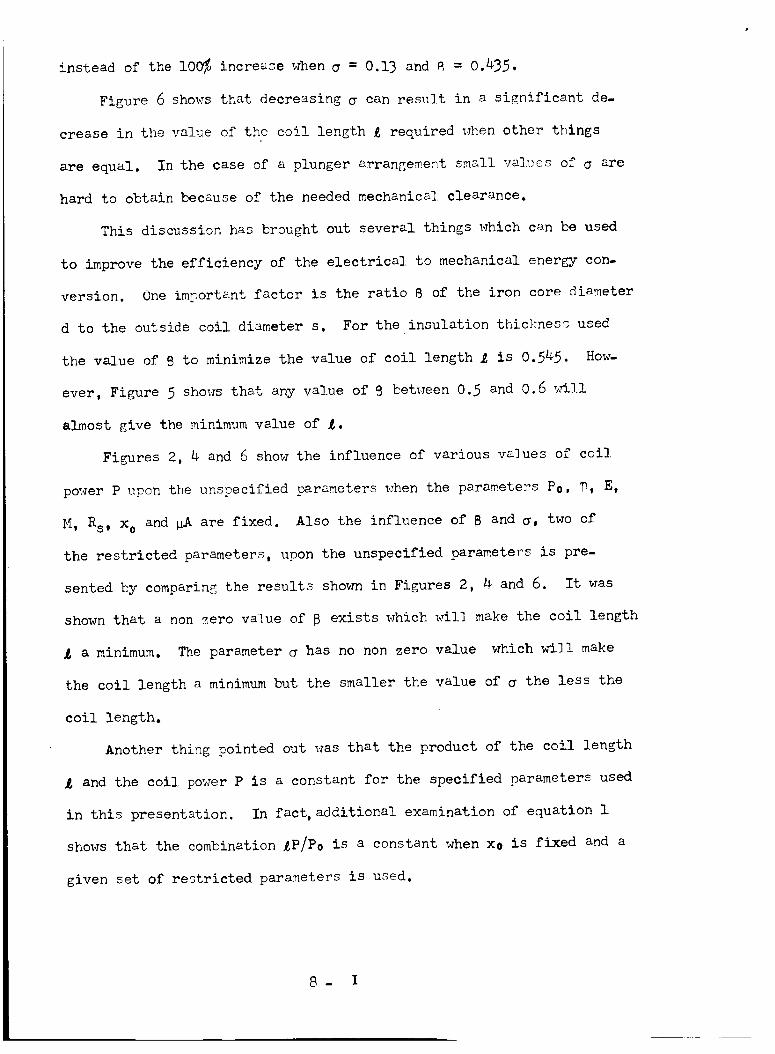
instead of the lO0%p increase when _ = 0.13 and g = 0.435.

Figure 6 shows that decreasing q can result in a significant de.

crease in the value of the coil length _ required _ff_en other things

are equal. In the case of a plunger arrangement small valises of _ are

hard to obtain because of the needed mechanical clearance.

This discussion has brought out several things which can be used

to improve the efficiency of the electrical to mechanical energy con-

version. One important factor is the ratio B of the iron core diameter

d to the outside coil diameter s. For the insulation thic_ness used

the value of B to minimize the value of coil length _ is 0.545. How-

ever, Figure 5 shows that any value of _ between 0.5 and 0.6 will

almost give the minimum value of _.

Figures 2, 4 and 6 show the influence of various values of coil

power P upon the unspecified parameters _<hen the parameters P0, P, E,

M, Rs, x 0 and _A are fixed. Also the influence of B and _, two of

the restricted parameters, upon the unspecified parameters is pre-

sented by comparing the results shown in Figures 2, 4 and 6. It was

shown that a non zero value of B exists which will make the coil length

a minimum. The parameter _ has no non zero value which will make

the coil length a minimum but the smaller the value of _ the less the

coil length.

Another thing pointed out was that the product of the coil length

and the coil power P is a constant for the specified parameters used

in this presentation. In fact, additional examination of equation 1

shows that the combination _P/P0 is a constant when xo is fixed and a

given set of restricted parameters is used.

8- I

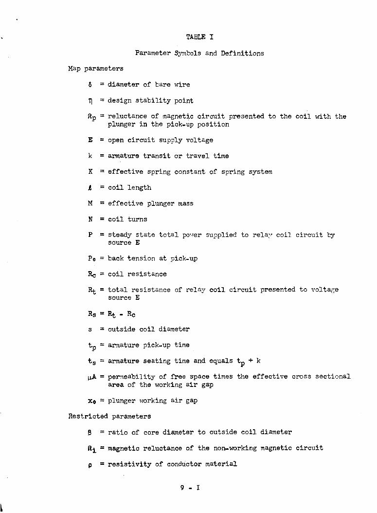
TABLE I

Parameter Symbols and Definitions

Map parameters


= design stability point

_p = reluctance of magnetic circuit presented to the coil with theplunger in the pick-up position

E = open circuit supply voltage

k = armature transit or travel time

K = effective spring constant of spring system

= coil length


N = coil turns

P = steady state total po_er supplied to rela_ coil circuit bysource E

Po = back tension at pick-up


Rt = total resistance of relay coil circuit presented to voltagesource E

Rs = Rt - Rc


tp = armature pick-up time

ts = armature seating time andequals tp + k

_A = permeability of free space times the effective cross sectional

area of the working air gap

Xe = plunger working air gap


8 = ratio of core diameter to outside coil diameter

_i = magnetic reluctance of the non-working magnetic circuit


9 - I

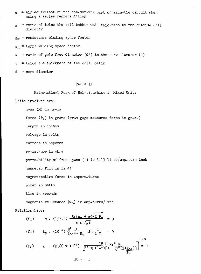
= air equivalent of the non-working part of magnetic circuit :_enusing a series representation

= ratio of twice the coil bobbin wall thickness to the outside coildiameter



a = ratio of pole face diameter (dt) to the core diameter (d)

u = twice the thickness of the coil bobbin

d = core diameter

TABLEII

Mathematical Form of Relationships in Mixed Units

Units involved are:

mass (M) in grams

force (P0) in grams (gram gage measures force in grams)

length in inches

voltage in volts

current in amperes

resistance in ohms

permeability of free space (_) is 3.19 lines/amp-turn inch

magnetic flmx in lines

magnetomotive force in ampere-turns

power in watts

time in seconds

magnetic reluctance (Rp) in amp-turns/line

Rt(x. + _-_Po=0

E

(f2) tp (I0-e) Nz j_A In _" (xo+_)P_ 1-_ --o

Relationships:

(f,) _ - (157.5)

(f3) k

1/3

I 18N ° P . (8.66 x I0-3) _ (I-9)[I _VZ('l+Kxo) = 0

Po

I0- I

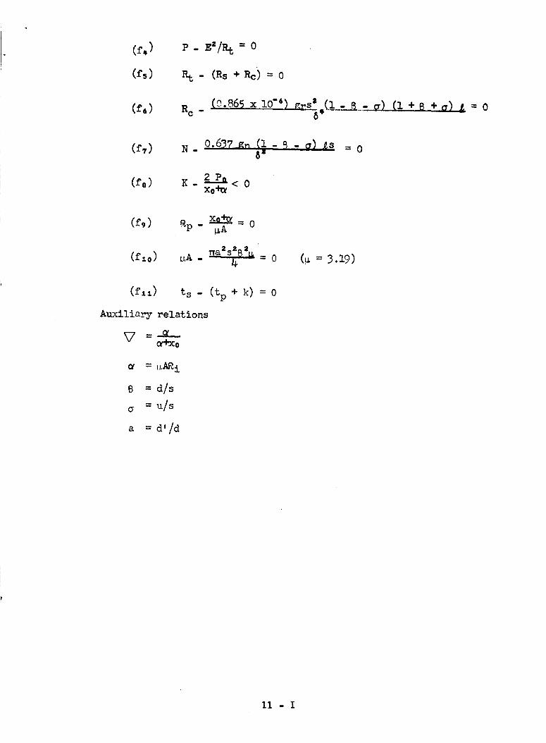
(f6)

P - E'/_ --o

- (Rs+ Re)- o

(0.865 x 10-6 ) _.rS' (I - _ - _) (I +Rc. . 8___=___ S +a) L = 0

(fT)

(f8)

0.637_n _I- B - a) _sN-

K. 2--_P< oxe+_

=0

(f,)

(f_o)

_p . X-_ = 0_A

,jA- _4 = 0 (_ - 3.19)

(f_1) ts - (tp

A_uxiliary relations

V =-q--a_xo

= I_A2i

8 = d/s

(y = U/S

a = d'/d

+k)=0

11 - I

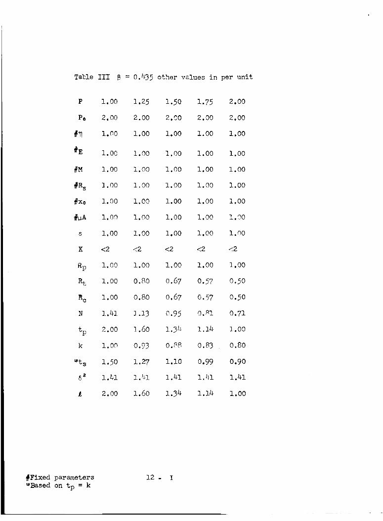
Table III = 0.I_35 other values in per unit

P 1.00 1.25 1.50 1.75 2.00

Po 2.00 2.00 2.00 2.00 2.00

_ 1.00 1.00 1.00 1.00 1.00

#E 1.00 1.00 1.00 1.00 1.00

_M 1.00 1.00 1.00 1.00 1.00

_Rs 1.00 1.00 1.00 1.00 1.00

#Xo 1.00 1.00 1.00 1.00 1.00

_A 1.0O 1.00 1.00 1.00 l.O0

s 1.00 1.00 1.00 1.00 l.O0

K <2 <2 <2 <2 <2

Rp i.O0 1.00 1.00 1.00 1.00

Rt 1.00 0.80 0.67 0.57 0.50

Rc 1.00 0.80 0.67 0.57 0.50

N 1.41 1.13 0.95 0.81 0.71

tp 2.00 ] .60 1.3_ 1.14 1.00

k 1.00 0.93 0._8 0.83 0.80

_t s 1.50 1.27 1.10 0.99 0.90

8z 1.41 1.41 1.41 1.41 1.41

2.00 1.60 1.34 1.14 1.00

#Fixed parameters_Based on tp = k

12- I

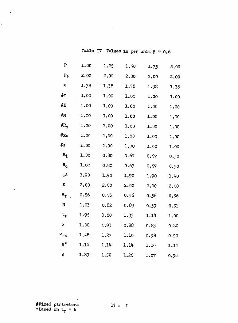
Table IV Values in per unit B = 0.6

P 1.O0 1.25 1.50 1.75 2.00

Po 2.00 2.00 2.00 2.00 2.00

8 1.38 1.38 1.38 1.38 1.38

#11 1.00 1.00 1.00 1.00 1.00

#E I. 00 i.00 I. 00 I. O0 i.00

#M I.O0 I. 00 I.00 I.00 I.O0

#R s I.00 I.00 i.00 I.00 I.00

#xe 1.00 1.00 1.00 1.00 1.00

#s I.oo 1.oo 1.oo i.oo i.oo

Rt 1.00 0.80 0.67 0.57 0.50

Rc 1.00 0.80 0.67 0.57 0.50

_A 1.90 1.90 1.90 1.90 1.90

K 2.O0 2.O0 2.O0 2.O0 2.oo

Rp 0.56 0.56 0.56 0.56 0.56

N 1.03 0.82 0.69 0.59 0.51

tp 1.95 1.60 1.33 1.14 1.00

k 1.00 0.93 0.88 0.83 0.80

_ts 1.48 1.27 1.10 0.98 0.90

6' 1.14 1.1_ 1.14 1.14 1.14

L 1.89 1.50 1.26 1.07 0.94

#Fixed parameters

_Based on tp = k

13- I

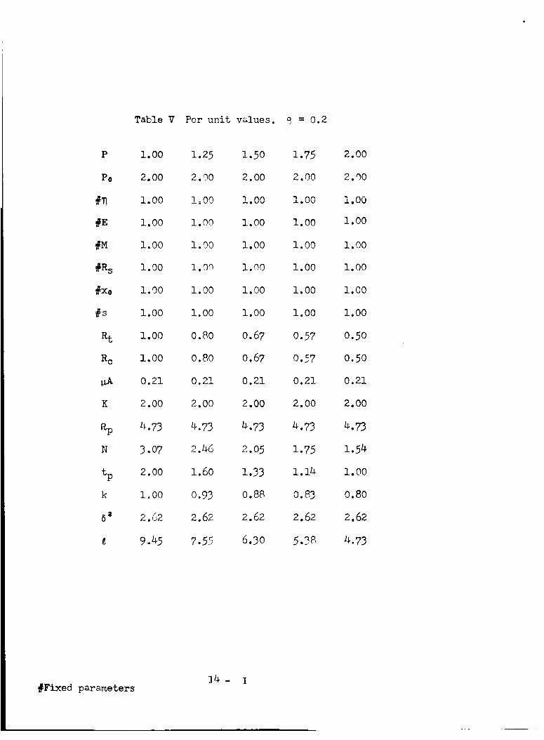
Table V Per unit values. _ = 0.2

P 1.00 1.25 1.50 1.75 2.00

Po 2.00 2.00 2.00 2.00 2.00

#_ 1.00 Inn _.nn , _^....... _._u i.00

#E 1.00 1.00 1.00 1.00 1.00

#M 1.00 1.00 1.00 1.00 1.00

#R s 1.00 1.00 1.00 1.00 1.00

#xo 1.00 1.00 1.00 1.00 1.00

#s 1.00 1.00 1.00 1.00 1.00

Rt 1.00 0.80 0.67 0.57 0.50

Rc 1.00 0.80 0.67 0.57 0.50

_A 0.21 0.21 0.21 0.21 0.21

K 2.00 2.00 2.00 2.00 2.00

_p 4.73 4.73 4.73 4.73 4.73

N 3.07 2.46 2.05 1.75 1.54

tp 2.00 1.60 1.33 1.14 1.00

k 1.00 0.93 0.88 0.83 0.80

6z 2.62 2.62 2.62 2.62 2.62

9.45 7.55 6.30 5.38 4.73

#Fixed parameters14- I

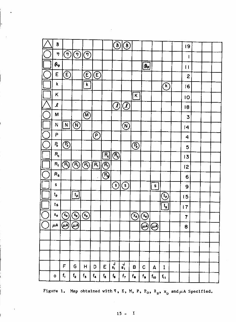
A _ ®® ,9O " ®@@1-1_ _ I "O_@ @@

l-1 '< _ ,o

O _ ®I---I",'® @ i® ,_O ,_ ® 40_@ @I-,-IRo _® ,_i--1_,® ® ®i_'® ,_ORs '@

I

l-q,, l_ @ ,_[3 ', ffa ,,O_'o®® ® ®® ',

,,I ,,1F 6 H D E $1 sl B C A I

o fl f2 f+ f4 f5 f6 f, fa f. f_o fll

Figure I. Map obtained wlthW, E, M, P, Po, Rs, xo and_A Specified.

15 - I

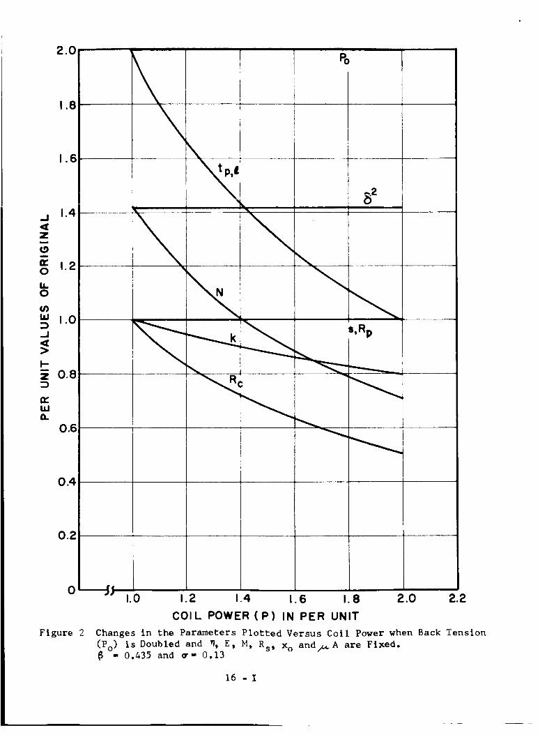
2.0

1.8

1.6

.j 1.4¢¢Zm

(,9m

¢ 1.20

14.0

U')w l.O

.-I

>

I-0.8

w

0.6

0.4

0.2

0

Figure 2

Po

..2

"3

,........_ _ s, Rp

1.0 1.2 .4 .6 1.8 2.0 2.2

COIL POWER (P) IN PER UNIT

Changes in the Parameters Plotted Versus Coil Power when Back Tension

(Po) is Doubled and _, E, M, Rs, Xo and_A are Fixed,- 0.435 and _- 0.13

16 -I

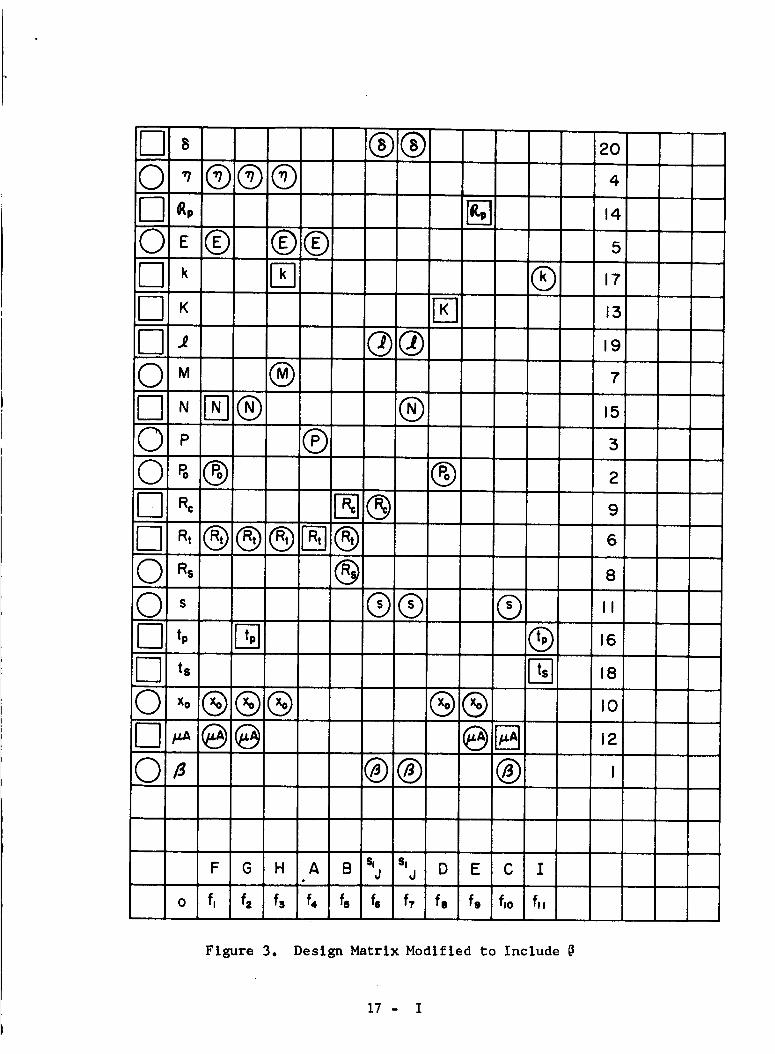
LI_ ®®0 ',@®®

U__J_/ -' @i®QM ®LN_® @Q,' ®Q_@iL _o 15J@ll ,,,@@6) _ 6)0 _, ®iO'

' I t,

0 ,o®®®LI _!@@0,_

®

®® ®

@(9

@1@ @

®

®t._%

2O

4

14

5

17

13

19

7

15

3

2

9

6

8

II

16

18

I0

12

I

0

F G H A B % s,• j j O E C I

f, f2 fs f4 f5 fe f7 fa f, f,o fl,

Figure 3. Design Matrix Modified to Include

17 - I

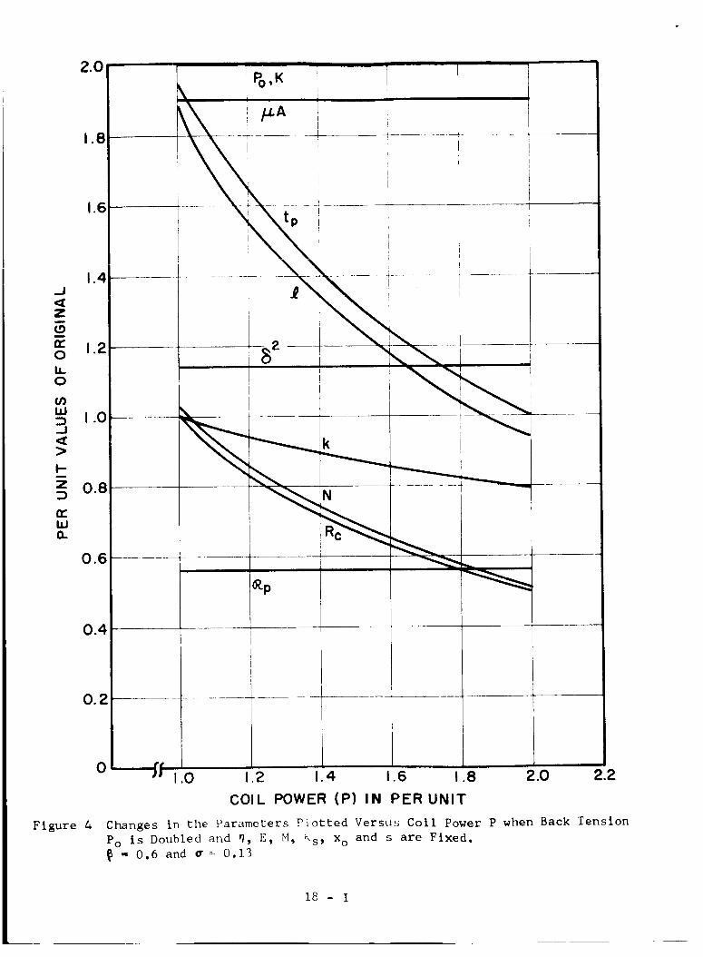
18

16

14J

Z

_9I

0

u.0

WI0

J

>

I

z 0.8D

IEhin

0.6

0.4

0.2

Figure 4

k

N

0

I;f I[.0 1.2 1.4 1.6 1.8 2.0 2.2


Changes in the Parameters Plotted Versus Coll Power P when Back Tension

Po is Doubled and 7, E, M, _s_ Xo and s are Fixed.

- 0.6 and _ = 0.13

I_ - I

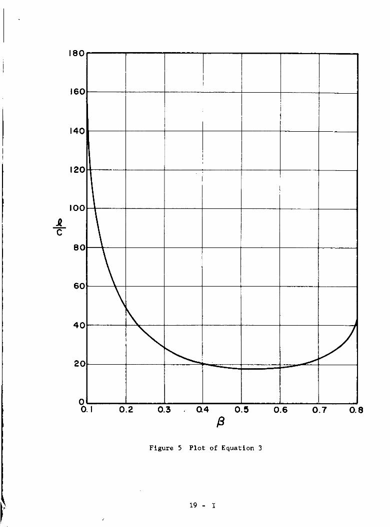
180

n

C

160

140

120

I00

80

60

40

20 J

00.1 0.2 0.3 Q4 0.5 0.6 0.7 0.8

Figure 5 Plot of Equation 3

19 - I

2.0

1.8

1.6

1.4_J

ZJ

0

U_0

,., 1.0

=,

.E o.8:)

1.1,,IQ.

0.6

0.4

0.2

0

Figure 6

I

\

k

R C

-----4f

7iI

1.0 1.2 1.4 1.6 1.8


2.0 22

Changes in tbc Parameters Plotted Versus Coll Power P when Back Tension

Po is Doubled and _, E, U, Rs, x o and s nre Fixed.

= 0.6 and _ _ 0.065

20 - I

Documents

,d POWER RELAY DESIGN - ntrs.nasa.gov · Reproduction of this document in any form ... It appears that some combination of increased coil power and ... There was a double hump immediately