D ORDER OPTIMIZATION USING K FACTORED … as a conference paper at ICLR 2017 DISTRIBUTED SECOND-ORDER OPTIMIZATION USING KRONECKER-FACTORED APPROXIMATIONS Jimmy Ba University of Toronto

Published as a conference paper at ICLR 2017

DISTRIBUTED SECOND-ORDER OPTIMIZATION USINGKRONECKER-FACTORED APPROXIMATIONS

Jimmy BaUniversity of [email protected]

Roger GrosseUniversity of [email protected]

James MartensUniversity of Torontoand Google [email protected]

ABSTRACT

As more computational resources become available, machine learning researcherstrain ever larger neural networks on millions of data points using stochastic gradi-ent descent (SGD). Although SGD scales well in terms of both the size of datasetand the number of parameters of the model, it has rapidly diminishing returns asparallel computing resources increase. Second-order optimization methods havean affinity for well-estimated gradients and large mini-batches, and can thereforebenefit much more from parallel computation in principle. Unfortunately, theyoften employ severe approximations to the curvature matrix in order to scale tolarge models with millions of parameters, limiting their effectiveness in practiceversus well-tuned SGD with momentum. The recently proposed K-FAC method(Martens and Grosse, 2015) uses a stronger and more sophisticated curvature ap-proximation, and has been shown to make much more per-iteration progress thanSGD, while only introducing a modest overhead. In this paper, we develop a ver-sion of K-FAC that distributes the computation of gradients and additional quan-tities required by K-FAC across multiple machines, thereby taking advantage ofthe method’s superior scaling to large mini-batches and mitigating its additionaloverheads. We provide a Tensorflow implementation of our approach which iseasy to use and can be applied to many existing codebases without modification.Additionally, we develop several algorithmic enhancements to K-FAC which canimprove its computational performance for very large models. Finally, we showthat our distributed K-FAC method speeds up training of various state-of-the-artImageNet classification models by a factor of two compared to an improved formof Batch Normalization (Ioffe and Szegedy, 2015).

1 INTRODUCTION

Current state-of-the-art deep neural networks (Szegedy et al., 2014; Krizhevsky et al., 2012; Heet al., 2015) often require days of training time with millions of training cases. The typical strategyto speed-up neural network training is to allocate more parallel resources over many machines andcluster nodes (Dean et al., 2012). Parallel training also enables researchers to build larger modelswhere different machines compute different splits of the mini-batches. Although we have improvedour distributed training setups over the years, neural networks are still trained with various simplefirst-order stochastic gradient descent (SGD) algorithms. Despite how well SGD scales with thesize of the model and the size of the datasets, it does not scale well with the parallel computationresources. Larger mini-batches and more parallel computations exhibit diminishing returns for SGDand related algorithms.

Second-order optimization methods, which use second-order information to construct updates thataccount for the curvature of objective function, represent a promising alternative. The canonicalsecond-order methods work by inverting a large curvature matrix (traditionally the Hessian), butthis doesn’t scale well to deep neural networks with millions of parameters. Various approximationsto the curvature matrix have been proposed to help alleviate this problem, such as diagonal (LeCunet al., 1998; Duchi et al., 2011; Kingma and Ba, 2014), block diagonal Le Roux et al. (2008),and low-rank ones (Schraudolph et al., 2007; Bordes et al., 2009; Wang et al., 2014; Keskar andBerahas, 2015; Moritz et al., 2016; Byrd et al., 2016; Curtis, 2016; Ramamurthy and Duffy). Another

1


strategy is to use Krylov-subspace methods and efficient matrix-vector product algorthms to avoidthe inversion problem entirely (Martens, 2010; Vinyals and Povey, 2012; Kiros, 2013; Cho et al.,2015; He et al., 2016).

The usual problem with curvature approximations, especially low-rank and diagonal ones, is thatthey are very crude and only model superficial aspects of the true curvature in the objective function.Krylov-subspace methods on the other hand suffer because they still rely on 1st-order methods tocompute their updates.

More recently, several approximations have been proposed based on statistical approximations of theFisher information matrix (Heskes, 2000; Ollivier, 2013; Grosse and Salakhutdinov, 2015; Poveyet al., 2015; Desjardins et al., 2015). In the K-FAC approach (Martens and Grosse, 2015; Grosseand Martens, 2016), these approximations result in a block-diagonal approximation to the Fisherinformation matrix (with blocks corresponding to entire layers) where each block is approximatedas a Kronecker product of two much smaller matrices, both of which can be estimated and invertedfairly efficiently. Because the inverse of a Kronecker product of two matrices is the Kroneckerproduct of their inverses, this allows the entire matrix to be inverted efficiently.

Martens and Grosse (2015) found that K-FAC scales very favorably to larger mini-batches comparedto SGD, enjoying a nearly linear relationship between mini-batch size and per-iteration progress formedium-to-large sized mini-batches. One possible explanation for this phenomenon is that second-order methods make more rapid progress exploring the error surface and reaching a neighborhood ofa local minimum where gradient noise (which is inversely proportional to mini-batch size) becomesthe chief limiting factor in convergence1. This observation implies that K-FAC would benefit inparticular from a highly parallel distributed implementation.

In this paper, we propose an asynchronous distributed version of K-FAC that can effectively ex-ploit large amounts of parallel computing resources, and which scales to industrial-scale neural netmodels with hundreds of millions of parameters. Our method augments the traditional distributedsynchronous SGD setup with additional computation nodes that update the approximate Fisher andcompute its inverse. The proposed method achieves a comparable per-iteration runtime as a normalSGD using the same mini-batch size on a typical 4 GPU cluster. We also propose a “doubly fac-tored” Kronecker approximation for layers whose inputs are feature maps that are normally too largeto handled by the standard Kronecker-factored approximation. Finally, we empirically demonstratethat the proposed method speeds up learning of various state-of-the-art ImageNet models by a factorof two over Batch Normalization (Ioffe and Szegedy, 2015).

2 BACKGROUND

2.1 KRONECKER FACTORED APPROXIMATE FISHER

Let DW be the gradient of the log likelihood L of a neural network w.r.t. some weight matrixW ∈ RCout×Cin in a layer, where Cin, Cout are the number of input/output units of the layer. Theblock of the Fisher information matrix of that layer is given by:

F = Ex,y∼P

[vec{DW} vec{DW}>

], (1)

where P is the distribution over the input x and the network’s distribution over targets y (impliedby the log-likelihood objective). Throughout this paper we assume, unless otherwise stated, thatexpectations are taken with respect to P (and not the training distribution over y).

K-FAC (Martens and Grosse, 2015; Grosse and Martens, 2016) uses a Kronecker-factored approx-imation to each block which we now describe. Denote the input activation vector to the layer asA ∈ RCin , the pre-activation inputs as s = WA and the back-propagated loss derivatives asDs = dL

ds ∈ RCout . Note that the gradient of the weights is the outer product of the input acti-vation and back-propagated derivatives DW = DsA>. K-FAC approximates the Fisher block as a

1Mathematical evidence for this idea can be found in Martens (2014), where it is shown that (convexquadratic) objective functions decompose into noise-dependent and independent terms, and that second-ordermethods make much more rapid progress optimizing the noise-independent term compared to SGD, while haveno effect on the noise-dependent term (which shrinks with the size of the mini-batch)

2


Kronecker product of the second-order statistics of the input and the backpropagated derivatives:

F =E[vec{DW} vec{DW}>

]= E

[AA> ⊗DsDs>

]≈ E

[AA>

]⊗ E

[DsDs>

], F . (2)

This approximation can be interpreted as making the assumption that the second-order statistics ofthe activations and the backpropagated derivatives are uncorrelated.

2.2 APPROXIMATE NATURAL GRADIENT USING K-FAC

The natural gradient (Amari, 1998) is defined as the inverse of the Fisher times the gradient. It istraditionally interpreted as the direction in parameter space that achieves the largest (instantaneous)improvement in the objective per unit of change in the output distribution of the network (as mea-sured using the KL-divergence). Under certain conditions, which almost always hold in practice,it can also be interpreted as a second-order update computed by minimizing a local quadratic ap-proximation of the log-likelihood objective, where the Hessian is approximated using the Fisher(Martens, 2014).

To compute the approximate natural gradient in K-FAC, one multiplies the gradient for the weightsof each layer by the inverse of the corresponding approximate Fisher block F for that layer. Denotethe gradient of the loss function with respect to the weights W by GW ∈ RCin×Cout . We willassume the use of the factorized Tikhonov damping approach described by Martens and Grosse(2015), where the addition of the damping term λI to F is approximated by adding πAλ

12 I to

E[AA>

]and πDsλ

12 I to E

[DsDs>

], where πA and πDs are adjustment factors that are described

in detail and generalized in Sec. 4.1. (Note that one can also include the contribution to the curvaturefrom any L2 regularization terms with λ.)

By exploiting the basic identities (A⊗B)−1 = (A−1⊗B−1) and (A⊗B) vec(C) = vec(BCA>),the approximate natural gradient update v can then be computed as:

v =(F + λI

)−1vec{GW } ≈ vec

{(E[AA>

]+ πAλ

12 I)−1GW

(E[DsDs>

]+ πDsλ

12 I)−1}

,

(3)

which amounts to several matrix inversion of multiplication operations involving matrices roughlythe same size as the weight matrix W .

3 DISTRIBUTED OPTIMIZATION USING K-FAC

Stochastic optimization algorithms benefit from low-variance gradient estimates (as might be ob-tained from larger mini-batches). Prior work suggests that approximate natural gradient algorithmsmight benefit more than standard SGD from reducing the variance (Martens and Grosse, 2015;Grosse and Martens, 2016). One way to efficiently obtain low-variance gradient estimates is to par-allelize the gradient computation across many machines in a distributed system (thus allowing largemini-batches to be processed efficiently). Because the gradient computation in K-FAC is identical tothat of SGD, we parallelize the gradient computation using the standard synchronous SGD model.

However, K-FAC also introduces other forms of overhead not found in SGD — in particular, estima-tion of second-order statistics and computation of inverses or eigenvalues of the Kronecker factors.In this section, we describe how these additional computations can be performed asynchronously.While this asynchronous computation introduces an additional source of error into the algorithm,we find that it does not significantly affect the per-iteration progress in practice. All in all, the per-iteration wall clock time of our distributed K-FAC implementation is only 5-10% higher comparedto synchronous SGD with the same mini-batch size.

3.1 ASYNCHRONOUS FISHER BLOCK INVERSION

Computing the parameter updates as per Eq.3 requires the estimated gradients to be multiplied bythe inverse of the smaller Kronecker factors. This requires periodically computing (typically) eitherinverses or eigendecompositions of each of these factors. While these factors typically have sizes

3


...

parameters

gradient worker

statsworker

parameter server

computeinverses

gradient worker

gradient worker

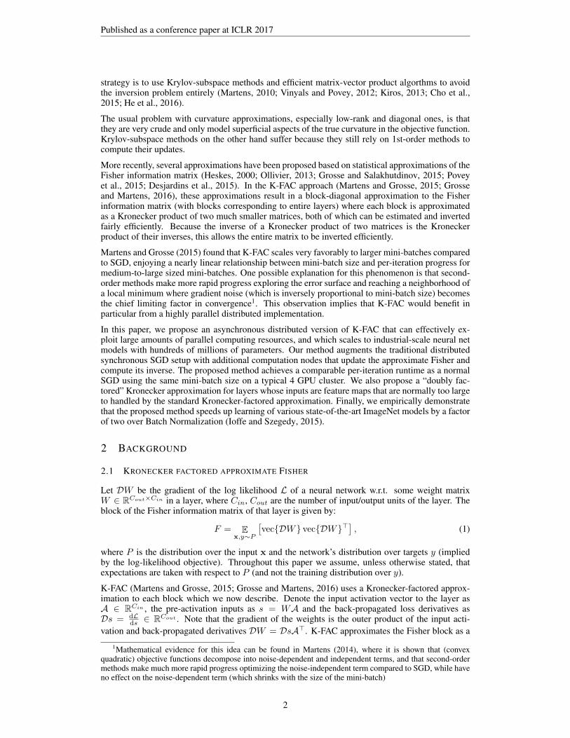
Figure 1: The diagram illustrates the distributed computation of K-FAC. Gradient workers (blue)compute the gradient w.r.t. the loss function. Stats workers (grey) compute the sampled second-order statistics. Additional workers (red) compute inverse Fisher blocks. The parameter server(orange) uses gradients and their inverse Fisher blocks to compute parameter updates.

only in the hundreds or low thousands, very deep networks may have hundreds of such matrices(2 or more for each layer). Furthermore, matrix inversion and eigendecomposition see little benefitfrom GPU computation, so they can be more expensive than standard neural network operations.For these reasons, inverting the approximate Fisher blocks represents a significant computationalcost.

It has been observed that refreshing the inverse of the Fisher blocks only occasionally and usingstale values otherwise has only a small detrimental effect on average per-iteration progress, perhapsbecause the curvature changes relatively slowly (Martens and Grosse, 2015). We push this a stepfurther by computing the inverses asynchronously while the network is still training. Because the re-quired linear algebra operations are CPU-bound while the rest of our computations are GPU-bound,we perform them on the CPU with little effective overhead. Our curvature statistics are somewhatmore stale as a result, but this does not appear to significantly affect per-iteration optimization per-formance. In our experiments, we found that computing the inverses asynchronously usually offereda 40-50% speed-up to the overall wall-clock time of the K-FAC algorithm.

3.2 ASYNCHRONOUS STATISTICS COMPUTATION

The other major source of computational overhead in K-FAC is the estimation of the second-orderstatistics of the activations and derivatives, which are needed for the Kronecker factors. In the stan-dard K-FAC algorithm, these statistics are computed on the same mini-batches as the gradients,allowing the forward pass computations to be shared between the gradient and statistics computa-tions. By computing the gradients and statistics on separate mini-batches, we can enable a higherdegree of parallelism, at the expense of slightly more total computational operations. Under thisscheme, the statistics estimation is independent of the gradient computation, so it can be done onone or more separate worker nodes with their own independent data shards. These worker nodesreceive parameters from the parameter server (just as in synchronous SGD) and communicate statis-tics back to the parameter server. In our experiments, we assigned at most one worker to computingstatistics.

In cases where it is undesirable to devote separate worker nodes to computing statistics, we alsointroduce a fast approximation to the statistics for convolution layers (see Appendix A).

4


4 DOUBLY-FACTORED KRONECKER APPROXIMATION FOR LARGECONVOLUTION LAYERS

Computing the standard Kronecker factored Fisher approximation for a given layer involves opera-tions on matrices whose dimension is the number of input units or output units. The cost of theseoperations is reasonable for most fully-connected networks because the number of units in each layerrarely exceeds a couple thousand. Large convolutional neural networks, however, often include afully-connected layer that “pools” over a large feature map before the final softmax classification.For instance, the output of the last pooling layer of AlexNet is of size 6 × 6 × 256 = 9216, whichthen provides inputs to the subsequent fully connected layer of 4096 ReLUs. VGG models alsoshare a similar architecture. For the standard Kronecker-factored approximation one of the factorswill be a matrix of size 9216 × 9216, which is too expensive to be explicitly inverted as often as isneeded during training.

In this section we propose a “doubly-factored” Kronecker approximation for layers whose input isa large feature map. Specifically, we approximate the second-order statistics matrix of the inputs asitself factoring as a Kronecker product. This gives an approximation which is a Kronecker productof three matrices.

Using the AlexNet example, the 9216 × 4096 weight matrix in the first fully connected layer isequivalent to a filterbank of 4096 filters with kernel size 6 × 6 on 256 input channels. Let A be amatrix of dimension T -by-Cin representing the input activations (for a single training case), whereT = Kw ×Kh is the feature map height and width, and Cin is the number of input channels. TheFisher block for such a layer can be written as:

E[vec{DW} vec{DW}>] = E[vec{A} vec{A}> ⊗DsDs>], A ∈ RT ×Cin . (4)

We begin be making the following rank-1 approximation:

A ≈ KΨ>, (5)

whereK ∈ RT , Ψ ∈ RCin are the factors along the spatial location dimension and the input channeldimension. The optimal solution of a low-rank approximation under the Frobenius norm is givenby the singular value decomposition. The activation matrix A is small enough that its SVD can becomputed efficiently. Let σ1, u1, v1 be the first singular value and its left and right singular vectorsof the activation matrix A, respectively. The factors of the rank-1 approximation are then chosen tobe K =

√σ1u1 and Ψ =

√σ1v1. K captures the activation patterns across spatial locations in a

feature map and Ψ captures the pattern across the filter responses. Under the rank-1 approximationof A we have:

E[vec{A} vec{A}> ⊗DsDs>] ≈ E[vec{KΨ>} vec{KΨ>}> ⊗DsDs>] (6)

= E[KK> ⊗ΨΨ> ⊗DsDs>]. (7)

We further assume the second order statistics are three-way independent between the loss derivativesDs, the activations along the input channels Ψ, and the activations along spatial locations K:

E[vec{DW} vec{DW}>] ≈ E[KK>]⊗ E[ΨΨ>]⊗ E[DsDs>]. (8)

The final approximated Fisher block is a Kronecker product of three small matrices. And note thatalthough we assumed the feature map activations have low-rank structure, the resulting approxi-mated Fisher is not low-rank.

The approximate natural gradient for this layer can then be computed by multiplying the inversesof each of the smaller matrices against the respective dimensions of the gradient tensor. We definea function Ri : Rd1×d2×d3 → Rdjdk×di that constructs a matrix from a 3D tensor by “reshap-ing” it so that the desired target dimension i ∈ {1, 2, 3} maps to columns, while the remainingdimensions (j and k) are “folded together” and map to the rows. Given the gradient of the weights,GW ∈ RT ×Cin×Cout we can compute the matrix-vector product with the inverse double-factoredKronecker approximated Fisher block as:

R−13

(E[DsDs>]−1R3

(R−12

(E[ΨΨ>]−1R2(R−11 (E[KK>]−1R1(GW )))

))). (9)

5


which is a nested application of the reshape function R(·) at each of the dimension of the gradienttensor.

The doubly factored Kronecker approximation provides a computationally feasible alternative to thestandard Kronecker-factored approximation for layers that have a number of parameters in the orderof hundreds of millions. For example, inverting it for the first fully connected layer of AlexNet takesabout 15 seconds on an 8 core Intel Xeon CPU, and such time is amortized in our asynchronousalgorithm.

Unfortunately, the homogeneous coordinate formulation is no longer applicable under this new ap-proximation. Instead, we lump the bias parameters together and associate a full Fisher block withthem, which can be explicitly computed and inverted since the number of bias parameters per layeris small.

4.1 FACTORED TIKHONOV DAMPING FOR THE DOUBLE-FACTORED KRONECKERAPPROXIMATION

In second-order optimization methods, “damping” performs the crucial task of correcting for theinaccuracies of the local quadratic approximation of the objective that is (perhaps implicitly) op-timized when computing the update (Martens and Sutskever, 2012; Martens, 2014, e.g.). In thewell-known Tikhonov damping/regularization approach, one adds a multiple of the identity λI tothe Fisher before inverting it (as one also does for L2-regularization / weight-decay), which roughlycorresponds to imposing a spherical trust-region on the update.

The inverse of a Kronecker product can be computed efficiently as the Kronecker product of theinverse of its factors. Adding a multiple of the identity complicates this computation (although itcan still be performed tractably using eigendecompositions). The “factored Tikhonov damping”technique proposed in (Martens and Grosse, 2015) is appealing because it preserves the Kroneckerstructure of the factorization and thus the inverse can still be computed by inverting each of thesmaller matrices (and avoiding the more expensive eigendecomposition operation). And in ourexperiments with large ImageNet models, we also observe the factored damping seems to performbetter in practice. In this subsection we derive a generalized version of factored Tikhonov dampingfor the double-factored Kronecker approximation.

Suppose we wish to add λI to our approximate Fisher block A⊗B ⊗ C. In the factored Tikhonovscheme this is approximated by adding πaλ

13 I , πbλ

13 I , and πcλ

13 I to A, B and C respectively, for

non-negative scalars πa, πb and πc satisfying πaπbπc = 1. The error associated with this approxi-mation is:

(A+ πaλ13 I)⊗ (B + πbλ

13 I)⊗ (C + πcλ

13 I)− (A⊗B ⊗ C + λI) (10)

=πcλ13 I ⊗A⊗B + πbλ

13 I ⊗A⊗ C + πaλ

13 I ⊗B ⊗ C

+ πcλi3 I ⊗ πbλ

13 I ⊗A+ πcλ

13 I ⊗ πaλ

13 I ⊗B + πaλ

13 I ⊗ πbλ

13 I ⊗ C (11)

Following Martens and Grosse (2015), we choose πa, πb and πc by taking the nuclear norm inEq. 11 and minimizing its triangle inequality-derived upper-bound. Note that the nuclear norm ofKronecker products is the product of the nuclear norms of each individual matrices: ‖A ⊗ B‖∗ =‖A‖∗‖B‖∗. This gives the following formula for the value of πa

πa =3

√(‖A‖∗dA

)2(‖B‖∗dB

‖C‖∗dC

)−1. (12)

where the d’s are the number of rows (equiv. columns) of the corresponding Kronecker factor ma-trices. The corresponding formulae for πb and πc are analogous. Intuitively, the Eq. 12 rescalesthe contribution to each factor matrix according to the geometric mean of the ratio of its norm vsthe norms of the other factor matrices. This results in the contribution being upscaled if the factor’snorm is larger than averaged norm, for example. Note that this formula generalizes to Kroneckerproducts of arbitrary numbers of matrices as the geometric mean of the norm ratios.

6


5 STEP SIZE SELECTION

Although Grosse and Martens (2016) found that Polyak averaging (Polyak and Juditsky, 1992) ob-viated the need for tuning learning rate schedules on some problems, we observed the choice oflearning rate schedules to be an important factor in our ImageNet experiments (perhaps due to higherstochasticity in the updates). On ImageNet, it is common to use a fixed exponential decay schedule(Szegedy et al., 2014; 2015). As an alternative to learning rate schedules, we instead use curvatureinformation to control the amount by which the predictive distribution is allowed to change aftereach update. In particular, given a parameter update vector v, the second-order Taylor approxima-tion to the KL divergence between the predictive distributions before and after the update is givenby the (squared) Fisher norm:

DKL[q||p] ≈ 1

2v>Fv (13)

This quantity can be computed with a curvature-vector product (Schraudolph, 2002). Observe thatchoosing a step size of η will produce an update with squared Fisher norm η2 v>Fv. Instead ofusing a learning rate schedule, we choose η in each iteration such that the squared Fisher norm is atmost some value c:

η = min

(ηmax,

√c

v>Fv

)(14)

Grosse and Martens (2016) used this method to clip updates at the start of training, but we foundit useful to use it throughout training. We use an exponential decay schedule ck = c0ζ

k, wherec0 and ζ are tunable parameters, and k is incremented periodically (every half an epoch in ourImageNet experiments). Shrinking the maximum changes in the model prediction after each updateis analogous to shrinking the trust region of the second-order optimization. In practice, computingcurvature-vector products after every update introduces significant computational overhead, so weinstead used the approximate Fisher F in place of F , which allows the approximate Fisher norm tobe computed efficiently as v>Fv = v>F (F−1GW ) = v>GW . The maximum step size ηmax wasset to a large value, and in practice this maximum was reached only at the beginning of training,when F was small in magnitude. We found this outperformed simple exponential learning ratedecay on ImageNet experiments (see Appendix B).

6 EXPERIMENTS

We experimentally evaluated distributed K-FAC on several large convolutional neural network train-ing tasks involving the CIFAR-10 and ImageNet classification datasets.

Due to computational resource constraints, we used a single GPU server with 8 Nvidia K80 GPUsto simulate a large distributed system. The GPUs were used as gradient workers that computed thegradient over a large mini-batch, with the CPUs acting as a parameter server. The Fisher blockinversions were performed on the CPUs in parallel, using as many threads as possible. The second-order statistics required for the various Fisher block approximations were computed either syn-cronously by the gradient workers after each gradient computation (CIFAR-10 experiments), orasynchronously using a separate dedicated “stats worker” (ImageNet experiments).

Meta-parameters such as learning rates, damping parameters, and the decay-rate for the second-order statistics, were optimized carefully by hand for each method. The momentum was fixed to0.9.

Similarly to Martens and Grosse (2015), we applied an exponentially decayed Polyak averagingscheme to the sequence of output iterates produced by each method. We found this improved theirconvergence rate in the later stages of optimization, and reduced or eliminated the need to decay thelearning rates.

We chose to base our implementation of distributed K-FAC on the TensorFlow framework (Abadiet al., 2016) because it provides well-engineered and scalable primitives for distributed computation.We implement distributed K-FAC in TensorFlow by scanning the gradient-computing graph forgroups of parameters whose gradient computations have particular structures. Having identified suchgroups we compute/approximate their Fisher blocks using a method tailored to the type of structure

7


0 500 1000 1500 2000 2500 3000Updates

0.40.60.81.01.21.41.6

NLL

dist.K-FAC async gpu1dist.K-FAC async gpu4dist.K-FAC sync gpu1dist.K-FAC sync gpu4

0 100 200 300 400 500 600sec.

0.40.60.81.01.21.41.6

NLL

0 500 1000 1500 2000 2500 3000Updates

0.00

0.05

0.10

0.15

0.20

0.25

0.30

Err.

0 100 200 300 400 500 600sec.

0.00

0.05

0.10

0.15

0.20

0.25

0.30

Err.

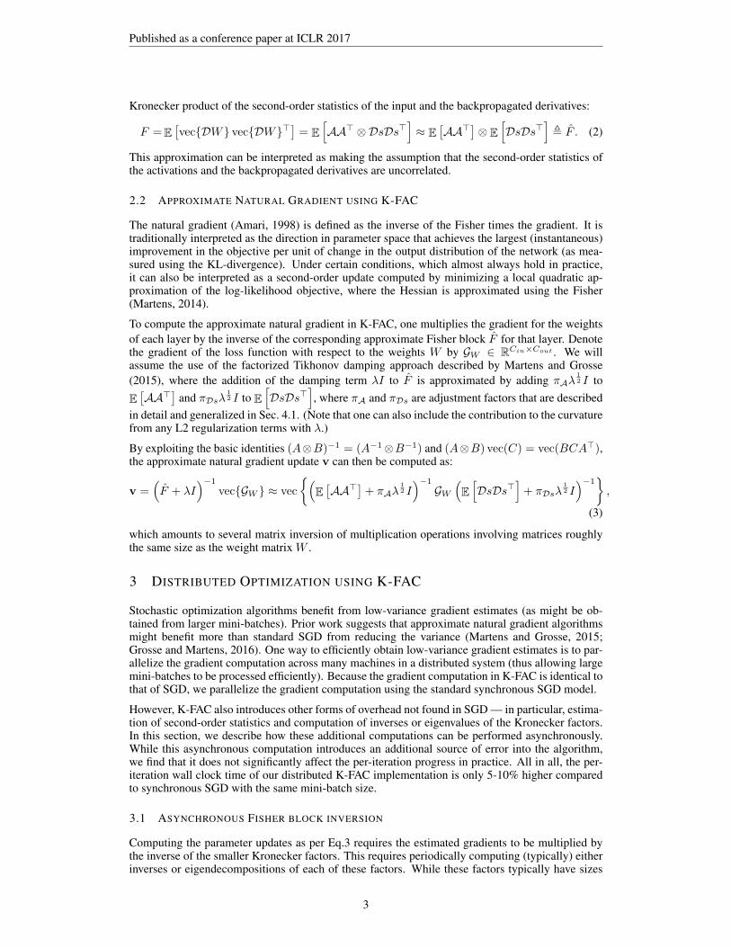
Figure 2: The results from our CIFAR-10 experiment looking at the effectiveness of asynchronouslycomputing the approximate Fisher inverses. gpu indicates the number of gradient workers. Dashedlines denote training curves and solid lines denote test curves. Top row: cross entropy loss andclassification error vs the number of updates. Bottom row: cross entropy loss and classificationerror vs wallclock time.

observed. See Appendix C for details. This type of implementation can be applied to existing model-specification code without significant modification of said code. And because TensorFlow’s parallelprimitives were designed with scalability in mind, it should be possible to scale our implementationto a larger distributed system with hundreds of workers.

6.1 CIFAR-10 CLASSIFICATION AND ASYNCHRONOUS FISHER BLOCK INVERSION

In our first experiment we evaluated the effectiveness of asynchronously computing the approximateFisher inverses (as described in Section 3.1). We considered the effect that this has both on thequality of the updates, as measured by per-iteration progress on the objective, and on the averageper-iteration wall-clock time.

The task is to train a basic convolutional network model on the CIFAR-10 image classificationdataset (Krizhevsky and Hinton, 2009). The model has 3 convolutional layers of 32-32-64 filters,each with a receptive field size of 5x5, followed by a softmax layer that predicts 10 classes. This isa similar but not identical CIFAR-10 model that was used by Grosse and Martens (2016). All theCIFAR-10 experiments use a mini-batch size of 512.

The baseline method is a simple synchronous version of distributed K-FAC with a fixed learningrate, and up to 4 GPUs acting as gradient and stats workers, which recomputes the inverses of theapproximate Fisher blocks once every 20 iterations. This baseline method behaves similarly to theimplementation of K-FAC in Grosse and Martens (2016), while being potentially faster due to itsgreater use of parallelism. We compare this baseline to a version of distributed K-FAC where theapproximate Fisher blocks are inverted asynchronously and in parallel with the rest of the optimiza-tion process. Note that under this scheme, inverses are updated about once every 16 iterations forthe single GPU condition, and every 30 iterations for the four GPU condition. For networks largerthan this relatively small CIFAR-10 net they may get updated (far) less often (e.g. the AlexNetexperiments in Section 6.2.2).

The results of this first experiment are plotted in Fig. 2. We found that the asynchronous versioniterated about 1.5 times faster than the synchronous version, while its per-iteration progress remainedcomparable. The plots show that the asynchronous version is better at taking advantage of parallelcomputation and displayed an almost linear speed-up as the number of gradient workers increasesto 4. In terms of the wall-clock time, using only 4 GPUs the asynchronous version of distributedK-FAC is able to complete 700 iterations in under a minute, where it achieves the minimum testerror (19%).

6.2 IMAGENET CLASSIFICATION

In our second set of experiments we benchmarked distributed K-FAC against several other popularapproaches, and considered the effect of mini-batch size on per-iteration progress. To do this wetrained various off-the-shelf convnet architectures for image classification on the ImageNet dataset

8


0 2 4 6 8 10 12 14 16Updates x 1e+04

1.01.52.02.53.03.54.04.5

Cros

sEnt

ropy

SGD+BN bz256 rbz128SGD+BN bz256 rbz32dist.K-FAC bz256dist.K-FAC+BN bz256

0 13.9 27.8 41.7 55.6 69.4 83.3 97.2hours

1.01.52.02.53.03.54.04.5

Cros

sEnt

ropy

0 2 4 6 8 10 12 14 16Updates x 1e+04

0.25

0.30

0.35

0.40

0.45

0.50

Err.

0 13.9 27.8 41.7 55.6 69.4 83.3 97.2hours

0.25

0.30

0.35

0.40

0.45

0.50

Err.

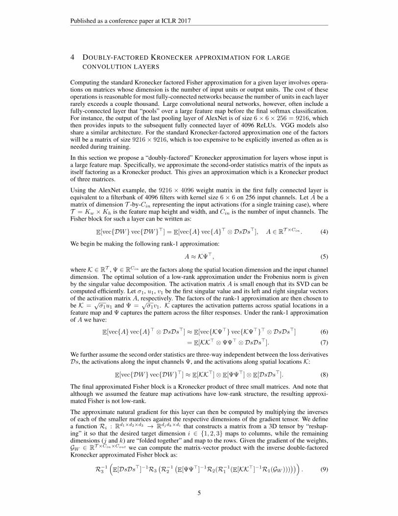
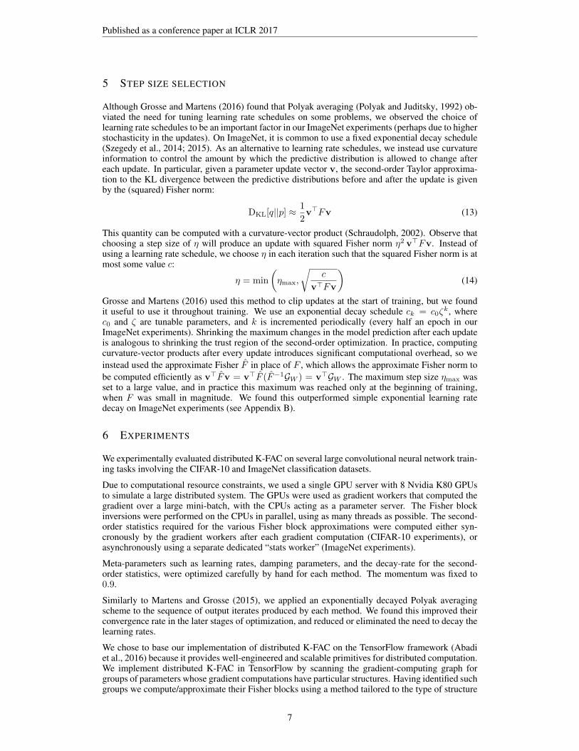
Figure 3: Optimization performance of distributed K-FAC and SGD training GoogLeNet on Ima-geNet. Dashed lines denote training curves and solid lines denote validation curves. bz indicates thesize of mini-batches. rbz indicates the size of chunks used to assemble the BN updates. Top row:cross entropy loss and classification error v.s. the number of updates. Bottom row: cross entropyloss and classification error vs wallclock time (in hours). All methods used 4 GPUs, with distributedK-FAC using the 4-th GPU as a dedicated asynchronous stats worker.

(Russakovsky et al., 2015): AlexNet (Krizhevsky et al., 2012), GoogLeNet InceptionV1 (Szegedyet al., 2014) and the 50-layer Residual network (He et al., 2015).

Despite having 1.2 million images in the ImageNet training set, a data pre-processing pipeline isalmost always used for training ImageNet that includes image jittering and aspect distortion. Weused a less extensive dataset augmentation/pre-processing pipeline than is typically used for Ima-geNet, as the purpose of this paper is not to achieve state-of-the-art ImageNet results, but ratherto evaluate the optimization performance of distributed K-FAC. In particular, the dataset consistsof 224x224 images and during training the original images are first resized to 256x256 and thenrandomly cropped back down to 224x224 before being fed to the network. Note that while it istypically the case that validation error is higher than training error, this data pre-processing pipelinefor ImageNet creates an augmented training set that is more difficult than the undistorted validationset and therefore the validation error is often lower than the training error during the first 90% oftraining. This observation is consistent with previously published results (He et al., 2015).

In all our ImageNet experiments, we used the cheaper Kronecker factorization from Appendix A,and the KL-based step sized selection method described in Section 5 with parameters c0 = 0.01and ζ = 0.96. The SGD baselines use an exponential learning rate decay schedule with a decayrate of 0.96. Decaying is applied after each half-epoch for distributed K-FAC and SGD+BatchNormalization, and after every two epochs for plain SGD, which is consistent with the experimentalsetup of Ioffe and Szegedy (2015).

6.2.1 GOOGLELENET AND BATCH NORMALIZATION

Batch Normalization (Ioffe and Szegedy, 2015) is a reparameterization of neural networks that canmake them easier to train with first-order methods, and has been successfully applied to large Ima-geNet models. It can be thought of as a modification of the units of a neural network so that eachone centers and normalizes its own raw input over the current mini-batch (or subset thereof), afterwhich it applies a separate shift and scaling operation via its own local “bias” and “gain” parameters(which are optimized). These shift and scaling operations can learn to effectively undo the center-ing and normalization, thus preserving the class of functions that the network can compute. BatchNormalization (BN) is closely related to centering techniques (Schraudolph, 1998), and likely helpsfor the same reason that they do, which is that the alternative parameterization gives rise to losssurfaces with more favorable curvature properties. The main difference between BN and traditionalcentering is that BN makes the centering and normalization operations part of the model insteadof the optimization algorithm (and thus “backprops” through them when computing the gradient),which helps stabilize the optimization.

Without any changes to the algorithm, distributed K-FAC can be used to train neural networks thathave BN layers. The weight-matrix gradient for such layers has the same structure as it does forstandard layers, and so Fisher blocks can be approximated using the same set of techniques. The

9


0 0.5 1 1.5 2 2.5 3 3.5 4 4.5Updates x 1e+04

1.01.52.02.53.03.54.04.55.0

Cros

sEnt

ropy

SGD bz2048 SGD+BN bz2048 rbz256dist.K-FAC bz2048

0 5.6 11.1 16.7 22.2 27.8 33.3hours

1.01.52.02.53.03.54.04.55.0

Cros

sEnt

ropy

0 0.5 1 1.5 2 2.5 3 3.5 4 4.5Updates x 1e+04

0.40

0.45

0.50

0.55

0.60

0.65

0.70

Err.

0 5.6 11.1 16.7 22.2 27.8 33.3hours

0.40

0.45

0.50

0.55

0.60

0.65

0.70

Err.

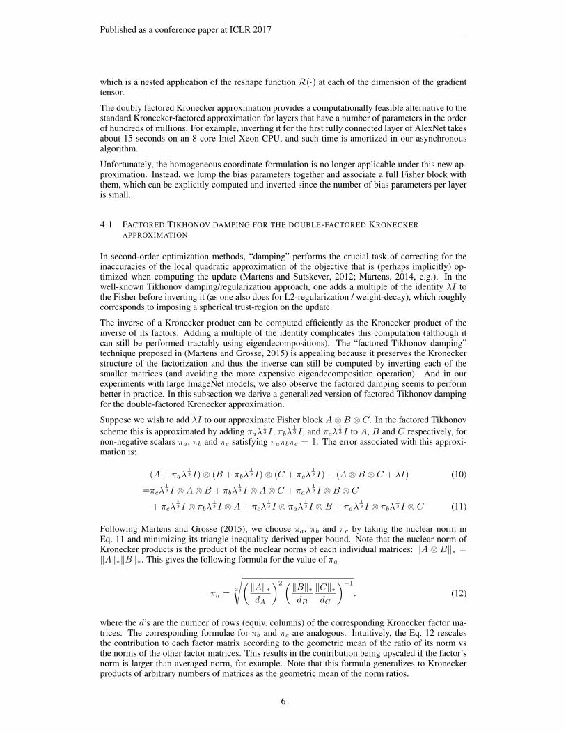
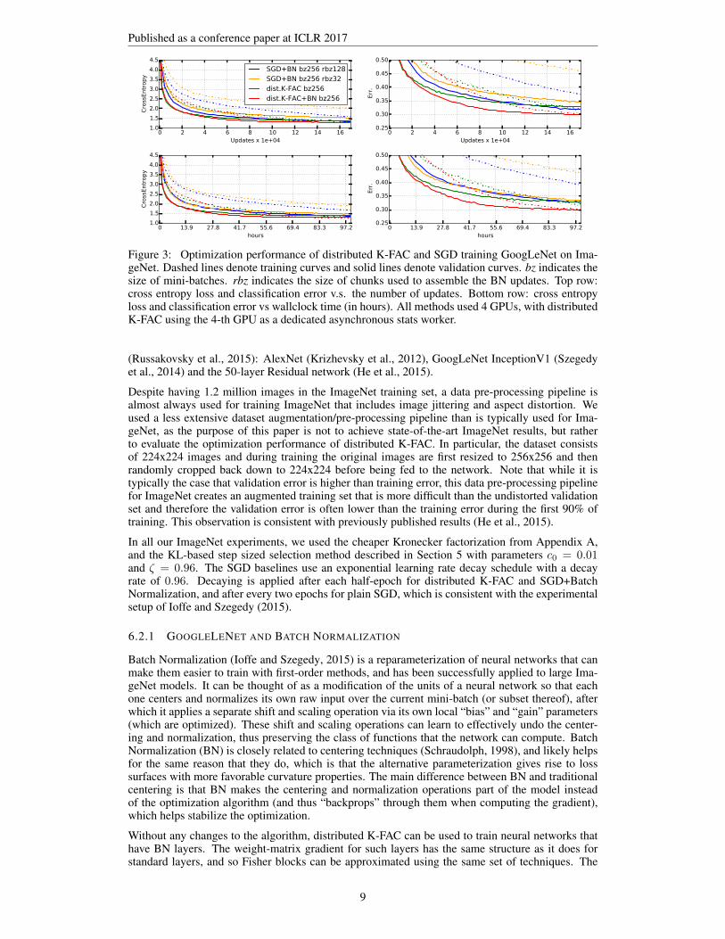
Figure 4: Optimization performance of distributed K-FAC and SGD training AlexNet on ImageNet.Dashed lines denote training curves and solid lines denote validation curves. bz indicates the sizeof the mini-batches. rbz indicates the size of chunks used to assemble the BN updates. Top row:cross entropy loss and validation error vs the number of updates. Bottom row: cross entropy lossand validation error vs wallclock time (in hours). All methods used 8 GPUs, with distributed K-FACusing the 8-th GPU as a dedicated asynchronous stats worker.

per-unit gain and bias parameters cause a minor complication, but because they are relatively few innumber, one can compute an exact Fisher block for each of them.

Computing updates for BN networks over large mini-batches is usually done by splitting the mini-batch into chunks of size 32, computing the gradients separately for these chunks (using only thedata in the chunk to compute the mean and variance statistics), and then summing them together.Using small sample sets to compute the statistics like this introduces additional stochasticity into theBN update that acts as a regularizer, but can also hurt optimization performance. To help decouplethe effect of regularization and optimization, we also compared to a BN baseline that uses largerchunks. We found using larger chunks can give a factor of 2 speed-up in optimization performanceover the standard BN baseline. In our figures rbz will indicate the chunk size, which defaults 32 ifleft unspecified.

In Fig. 3, we compare distributed K-FAC to SGD on GoogLeNet with and without BN. All methodsused 4 GPUs, with distributed K-FAC using the 4-th GPU as a dedicated asynchronous stats worker.

We observe that the per-iteration progress made by distributed K-FAC on the training objective is notsignificantly affected by the use of BN. Moreover, distributed K-FAC is 3.5 times faster than SGDwith standard BN baseline (orange line) and 1.5-2 times faster than the enhanced BN baseline (blueline). BN, however, does help distributed K-FAC generalize better, likely due to its aforementionedregularizing effect.

For the simplicity of our discussion, distributed K-FAC is not combined with BN in the the rest of theexperiments, as we are chiefly interested in evaluating optimization performance, not regularization,and BN doesn’t seem to provide any additional benefit to distributed K-FAC in regards to the former.Note that this is not too surprising, given that K-FAC is provably invariant to the kind of centeringand normalization transformations that BN does (Martens and Grosse, 2015).

6.2.2 ALEXNET AND THE DOUBLY-FACTORED KRONECKER APPROXIMATION

To demonstrate that distributed K-FAC can efficiently optimize models with very wide layers wetrain AlexNet using distributed K-FAC and compare to SGD+BN. The doubly-factored Kroneckerapproximation proposed in Section 4 is applied to the first fully-connected layer of AlexNet, whichhas 9216 input units and is thus too wide for the standard Kronecker approximation to be feasible.Note that even with this addtional approximation, computing all of the Fisher block inverses forAlexNet is very expensive, and in our experiments they only get updated once every few hundrediterations by our 16 core Xeon 2.2Ghz CPU.

The results from this experiment are plotted in Fig. 4. They show that Distributed K-FAC still workswell despite potentially extreme staleness of the Fisher block inverses, speeding up training by afactor of 1.5 over the improved SGD-BN baseline.

10


0 2 4 6 8 10 12Updates x 1e+04

1.01.52.02.53.03.54.04.55.0

Cros

sEnt

ropy

SGD+BN bz512 rbz64dist.K-FAC bz512

0 13.9 27.8 41.7 55.6 69.4 83.3 97.2hours

1.01.52.02.53.03.54.04.55.0

Cros

sEnt

ropy

0 2 4 6 8 10 12Updates x 1e+04

0.2

0.3

0.4

0.5

0.6

0.7

0.8

Err.

0 13.9 27.8 41.7 55.6 69.4 83.3 97.2hours

0.2

0.3

0.4

0.5

0.6

0.7

0.8

Err.

Figure 5: Optimization performance of distributed K-FAC and SGD training ResNet50 on Ima-geNet. The dashed lines are the training curves and solid lines are the validation curves. bz indicatesthe size of mini-batches. rbz indicates the size of chunks used to assemble the BN updates. Toprow: cross entropy loss and classification error v.s. the number of updates. Bottom row: cross en-tropy loss and classification error v.s. wallclock time (in hours). All methods used 8 GPUs, withdistributed K-FAC using the 8-th GPU as a dedicated asynchronous stats worker.

0 10 20 30 40 50#example consumed x 1e+06

1.0

1.2

1.4

1.6

1.8

2.0

2.2

2.4

Cros

sEnt

ropy

SGD+BN bz1024SGD+BN bz2048SGD+BN bz256dist.K-FAC bz1024dist.K-FAC bz2048dist.K-FAC bz256

0 10 20 30 40 50#example consumed x 1e+06

0.25

0.30

0.35

0.40

0.45

0.50

Trai

ning

Err

.

Figure 6: The comparison of distributed K-FAC and SGD on per training case progress on trainingloss and errors. The experiments were conducted using GoogLeNet with various mini-batch sizes.

6.2.3 VERY DEEP ARCHITECTURES (RESNETS)

In recent years very deep convolutional architectures have been successfully applied to ImageNetclassification. These networks are particularly challenging to train because the usual difficulties as-sociated with deep learning are especially severe. Fortunately second-order optimization is perhapsideally suited to addressing these difficulties in a robust and principled way (Martens, 2010).

To investigate whether distributed K-FAC can scale to such architectures and provide useful ac-celeration, we compared it to SGD+BN using the 50 layer ResNet architecture (He et al., 2015).The results from this experiment are plotted in Fig. 5. They show that distributed K-FAC providessignificant speed-up during the early stages of training compared to SGD+BN.

6.2.4 MINI-BATCH SIZE SCALING PROPERTIES

In our final experiment we explored how well distributed K-FAC scales as additional parallel com-puting resources become available. To do this we trained GoogLeNet with varying mini-batch sizesof {256, 1024, 2048}, and measured per-training-case progress. Ideally, if extra gradient data is be-ing used efficiently, one should expect the per-training-case progress to remain relatively constantwith respect to mini-batch size. The results from this experiment are plotted in Fig. 6, and showthat distributed K-FAC exhibits something close to this ideal behavior, while SGD+BN rapidly losesdata efficiency when moving beyond a mini-batch size of 256. These results suggest that distributedK-FAC, more so than the SGD+BN baseline, is capable of speeding up training in proportion to theamount of parallel computational resources used.

11


7 DISCUSSION

We have introduced distributed K-FAC, an asynchronous distributed second-order optimization al-gorithm which computes Kronecker-factored Fisher approximations and stochastic gradients overlarger mini-batches asynchronously and in parallel.

Our experiments show that the extra overhead introduced by distributed K-FAC is mostly mitigatedby the use of parallel asynchronous computation, resulting in updates that can be computed in asimilar amount of time to those of distributed SGD, while making much more progress on the ob-jective function per iteration. We showed that in practice this can lead to speedups of roughly 3.5xcompared to standard SGD + Batch Normalization (BN), and 2x compared to SGD + an improvedversion of BN on large-scale convolutional network training tasks.

We also proposed a doubly-factored Kronecker approximation that allows distributed K-FAC to scaleup to large models with hundreds of millions of parameters, and demonstrated the effectiveness ofthis approach in experiments.

Finally, we showed that distributed K-FAC enjoys a favorable scaling property with mini-batchsize that is seemingly not shared by SGD+BN. In particular, we showed that per-iteration progresstends to be proportional to the mini-batch size up to a much larger threshold than for SGD+BN. Thissuggests that it will yield even further reductions in total wall-clock training time when implementedin a larger distributed system than the one we considered.

REFERENCES

Martın Abadi, Ashish Agarwal, Paul Barham, Eugene Brevdo, Zhifeng Chen, Craig Citro, Greg S Corrado,Andy Davis, Jeffrey Dean, Matthieu Devin, et al. Tensorflow: Large-scale machine learning on heteroge-neous distributed systems. arXiv preprint arXiv:1603.04467, 2016.

Shun-Ichi Amari. Natural gradient works efficiently in learning. Neural computation, 10(2):251–276, 1998.

James Bergstra, Olivier Breuleux, Frederic Bastien, Pascal Lamblin, Razvan Pascanu, Guillaume Desjardins,Joseph Turian, David Warde-Farley, and Yoshua Bengio. Theano: A cpu and gpu math compiler in python.In Proc. 9th Python in Science Conf, pages 1–7, 2010.

Antoine Bordes, Leon Bottou, and Patrick Gallinari. Sgd-qn: Careful quasi-newton stochastic gradient descent.Journal of Machine Learning Research, 10(Jul):1737–1754, 2009.

Richard H Byrd, SL Hansen, Jorge Nocedal, and Yoram Singer. A stochastic quasi-newton method for large-scale optimization. SIAM Journal on Optimization, 26(2):1008–1031, 2016.

Minhyung Cho, Chandra Dhir, and Jaehyung Lee. Hessian-free optimization for learning deep multidimen-sional recurrent neural networks. In Advances in Neural Information Processing Systems, pages 883–891,2015.

Frank Curtis. A self-correcting variable-metric algorithm for stochastic optimization. In Proceedings of The33rd International Conference on Machine Learning, pages 632–641, 2016.

Jeffrey Dean, Greg Corrado, Rajat Monga, Kai Chen, Matthieu Devin, Mark Mao, Andrew Senior, Paul Tucker,Ke Yang, Quoc V Le, et al. Large scale distributed deep networks. In Advances in neural informationprocessing systems, pages 1223–1231, 2012.

Guillaume Desjardins, Karen Simonyan, Razvan Pascanu, and Koray Kavukcuoglu. Natural neural networks.In Advances in Neural Information Processing Systems, pages 2071–2079, 2015.

John Duchi, Elad Hazan, and Yoram Singer. Adaptive subgradient methods for online learning and stochasticoptimization. Journal of Machine Learning Research, 12(Jul):2121–2159, 2011.

Roger Grosse and James Martens. A kronecker-factored approximate fisher matrix for convolution layers. InProceedings of the 33rd International Conference on Machine Learning (ICML-16), 2016.

Roger Grosse and Ruslan Salakhutdinov. Scaling up natural gradient by factorizing fisher information. InProceedings of the 32nd International Conference on Machine Learning (ICML), 2015.

Kaiming He, Xiangyu Zhang, Shaoqing Ren, and Jian Sun. Deep residual learning for image recognition. arXivpreprint arXiv:1512.03385, 2015.

12


Xi He, Dheevatsa Mudigere, Mikhail Smelyanskiy, and Martin Takac. Large scale distributed hessian-freeoptimization for deep neural network. arXiv preprint arXiv:1606.00511, 2016.

Tom Heskes. On “natural” learning and pruning in multilayered perceptrons. Neural Computation, 12(4):881–901, 2000.

Sergey Ioffe and Christian Szegedy. Batch normalization: Accelerating deep network training by reducinginternal covariate shift. In Proceedings of The 32nd International Conference on Machine Learning, pages448–456, 2015.

Nitish Shirish Keskar and Albert S Berahas. adaqn: An adaptive quasi-newton algorithm for training rnns.arXiv preprint arXiv:1511.01169, 2015.

Diederik Kingma and Jimmy Ba. Adam: A method for stochastic optimization. arXiv preprintarXiv:1412.6980, 2014.

Ryan Kiros. Training neural networks with stochastic hessian-free optimization. arXiv preprintarXiv:1301.3641, 2013.

Alex Krizhevsky and Geoffrey Hinton. Learning multiple layers of features from tiny images. , University ofToronto, 2009.

Alex Krizhevsky, Ilya Sutskever, and Geoffrey E Hinton. Imagenet classification with deep convolutional neuralnetworks. In Advances in neural information processing systems, pages 1097–1105, 2012.

Nicolas Le Roux, Pierre-Antoine Manzagol, and Yoshua Bengio. Topmoumoute online natural gradient algo-rithm. In Advances in neural information processing systems, pages 849–856, 2008.

Yann LeCun, Leon Bottou, Yoshua Bengio, and Patrick Haffner. Gradient-based learning applied to documentrecognition. Proceedings of the IEEE, 86(11):2278–2324, 1998.

James Martens. Deep learning via Hessian-free optimization. In Proceedings of the 27th International Confer-ence on Machine Learning (ICML), pages 735–742, 2010.

James Martens. New insights and perspectives on the natural gradient method. arXiv preprint arXiv:1412.1193,2014.

James Martens and Roger Grosse. Optimizing neural networks with kronecker-factored approximate curvature.In Proceedings of the 32nd International Conference on Machine Learning (ICML-15), pages 2408–2417,2015.

James Martens and Ilya Sutskever. Training deep and recurrent networks with Hessian-free optimization. InNeural Networks: Tricks of the Trade, pages 479–535. Springer, 2012.

Philipp Moritz, Robert Nishihara, and Michael Jordan. A linearly-convergent stochastic L-BFGS algorithm. InProceedings of the 19th International Conference on Artificial Intelligence and Statistics, pages 249–258,2016.

Yann Ollivier. Riemannian metrics for neural networks i: feedforward networks. arXiv preprintarXiv:1303.0818, 2013.

Boris T Polyak and Anatoli B Juditsky. Acceleration of stochastic approximation by averaging. SIAM Journalon Control and Optimization, 30(4):838–855, 1992.

Daniel Povey, Xiaohui Zhang, and Sanjeev Khudanpur. Parallel training of DNNs with natural gradient andparameter averaging. In International Conference on Learning Representations: Workshop track, 2015.

Vivek Ramamurthy and Nigel Duffy. L-SR1: A novel second order optimization method for deep learning.

Olga Russakovsky, Jia Deng, Hao Su, Jonathan Krause, Sanjeev Satheesh, Sean Ma, Zhiheng Huang, An-drej Karpathy, Aditya Khosla, Michael Bernstein, et al. Imagenet large scale visual recognition challenge.International Journal of Computer Vision, 115(3):211–252, 2015.

Nicol N. Schraudolph. Centering neural network gradient factors. In Genevieve B. Orr and Klaus-RobertMuller, editors, Neural Networks: Tricks of the Trade, volume 1524 of Lecture Notes in Computer Science,pages 207–226. Springer Verlag, Berlin, 1998.

Nicol N. Schraudolph. Fast curvature matrix-vector products for second-order gradient descent. Neural Com-putation, 14(7), 2002.

13


Nicol N Schraudolph, Jin Yu, Simon Gunter, et al. A stochastic quasi-newton method for online convex opti-mization. In AISTATS, volume 7, pages 436–443, 2007.

Christian Szegedy, Wei Liu, Yangqing Jia, Pierre Sermanet, Scott Reed, Dragomir Anguelov, Dumitru Er-han, Vincent Vanhoucke, and Andrew Rabinovich. Going deeper with convolutions. arXiv preprintarXiv:1409.4842, 2014.

Christian Szegedy, Vincent Vanhoucke, Sergey Ioffe, Jonathon Shlens, and Zbigniew Wojna. Rethinking theinception architecture for computer vision. arXiv preprint arXiv:1512.00567, 2015.

Oriol Vinyals and Daniel Povey. Krylov subspace descent for deep learning. In AISTATS, pages 1261–1268,2012.

Xiao Wang, Shiqian Ma, and Wei Liu. Stochastic quasi-newton methods for nonconvex stochastic optimization.arXiv preprint arXiv:1412.1196, 2014.

14


0 1 2 3 4 5 6Updates x 1e+04

1.01.21.41.61.82.02.22.4

Cros

sEnt

ropy

dist.K-FAC KFC bz512dist.K-FAC fast bz512

0 13.9 27.8 41.7 55.6 69.4 83.3 97.2hours

1.01.21.41.61.82.02.22.4

Cros

sEnt

ropy

0 1 2 3 4 5 6Updates x 1e+04

0.25

0.30

0.35

0.40

0.45

0.50

Err.

0 13.9 27.8 41.7 55.6 69.4 83.3 97.2hours

0.25

0.30

0.35

0.40

0.45

0.50

Err.

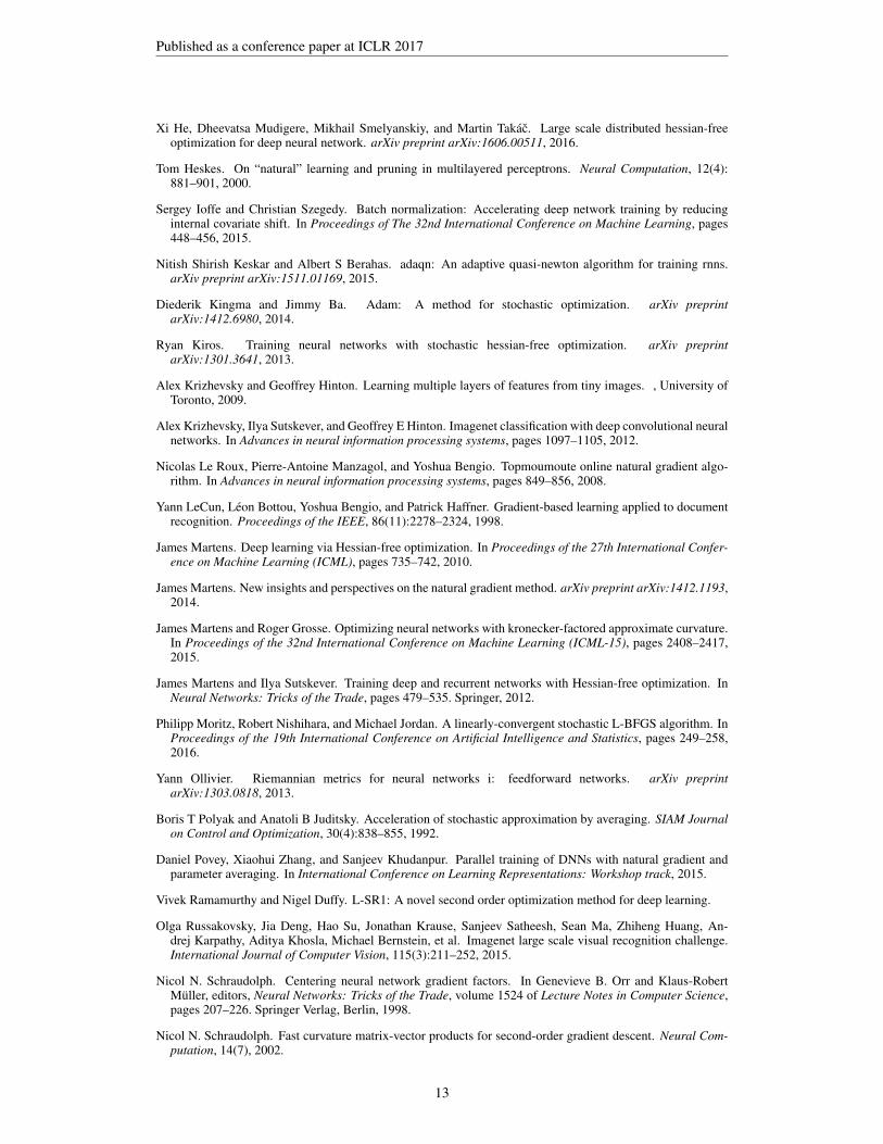
Figure 7: Empirical evaluation of the proposed cheaper Kronecker approximation on GoogLeNet.bz indicates the size of the mini-batches. Dashed lines denote training curves and solid lines denotevalidation curves. Top row: cross entropy loss and classification error vs the number of updates.Bottom row: cross entropy loss and classification error vs wallclock time.

A A CHEAPER KRONECKER FACTOR APPROXIMATION FOR CONVOLUTIONLAYERS

In a convolution layer, the gradient is the sum of the outer product between the receptive field inputactivation At and the back-propagated derivatives Dst at each spatial location t ∈ T . One cannotsimply apply the standard Kronecker factored approximation from Martens and Grosse (2015) toeach location, sum the results, and then take the inverse, as there is no known efficient algorithm forcomputing the inverse of such a sum.

In Grosse and Martens (2016), a Kronecker-factored approximation for convolutional layers calledKronecker Factors for Convolution (KFC) was developed. It works by introducing additional sta-tistical assumptions about how the weight gradients are related across locations. In particular, KFCassumes spatial homogeneity, i.e. that all locations have the same statistics, and spatially uncor-related derivatives, which (essentially) means that gradients from any two different locations arestatistically independent. This yields the following approximation:

E[vec{DW} vec{DW}>] ≈ |T |E[AtA>t

]⊗ E

[DstDs>t

]. (15)

In this section we introduce an arguably simpler Kronecker factored approximation for convolutionallayers that is cheaper to compute. In practice, it appears to be competitive with the original KFC ap-proximation in terms of per-iteration progress on the objective, working worse in some experimentsand better in others, while (often) improving wall-clock time due to its cheaper cost.

It works by approximating the sum of the gradients over spatial locations as the outer product ofthe averaged receptive field activations over locations Et[At], and the averaged back-propagatedderivatives Et[Dst], multipled by the number of spatial locations |T |. In other words:

E[vec{DW} vec{DW}>] = E

[vec{

∑t∈TDstA>t } vec{

∑t∈TDstA>t }>

](16)

=E

(∑t∈TAt ⊗Dst

)(∑t∈TAt ⊗Dst

)> (17)

≈E

[(|T |E

t[At]⊗ E

t[Dst]

)(|T |E

t[At]⊗ E

t[Dst]

)>](18)

Under the approximation assumption that the second-order statistics of the average activations,Et[At], and the second-order statistics of the average derivatives, Et[Dst], are uncorrelated, thisbecomes:

|T |2 E[Et[At]E

t[At]

>]⊗ E

[Et[Dst]E

t[Dst]>

](19)

15


0 0.5 1 1.5 2 2.5 3Updates x 1e+04

1.0

1.5

2.0

2.5

3.0

3.5

4.0

4.5

5.0

Cros

sEnt

ropy

dist.K-FAC bz256 decayKLdist.K-FAC bz256 decayLR

0 0.5 1 1.5 2 2.5 3Updates x 1e+04

0.40

0.45

0.50

0.55

0.60

0.65

0.70

Err.

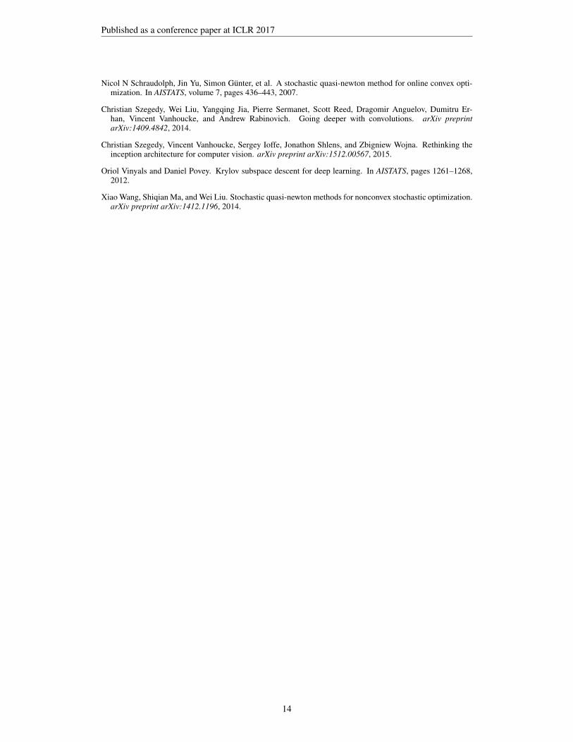
Figure 8: Results from the experiment described in Appendix B. decayKL indicates the proposedstep-size selection method and decayLR indicates standard exponential learning rate decay.

This approximation is cheaper than the original KFC approximation because it is easier to computea single outer product (after averaging over locations) than it is to compute an outer product ateach location and then average. In the synchronous setting, for the large convolutional networks weexperimented with, this trick resulted in a 20-30% decrease in overall wall clock time per iteration,with little effect on per-iteration progress.

B EXPERIMENTAL EVALUATION OF THE STEP-SIZE SELECTION METHOD OFSECTION 5

To compare our proposed step size selection from Sec. 5 with the commonly-used exponential learn-ing rate decay, we performed a simple experiment training GoogLeNet. Both the learning rate andthreshold c on the square Fisher norm, is decayed by a factor of 0.96 after every 3200 iterations.The results of this experiment are plotted in Fig. 8, and indicate that our method outperforms thestandard baseline.

C AUTOMATIC CONSTRUCTION OF THE K-FAC COMPUTATION GRAPH

In recent years, deep learning libraries have moved towards the computational graph abstraction(Bergstra et al., 2010; Abadi et al., 2016) to represent neural network computations. In this sectionwe give a high level description of an algorithm that scans a computational graph for parameters forwhich one of the various Kronecker-factored approximations can be applied, locates nodes contain-ing the required information to compute the second-order statistics required by the approximations,and then constructs a new graph that computes the approximations and uses them to update theparameters.

For the sake of discussion, we will assume the computation graph is a directed bipartite graph thathas a set of operator nodes doing some computation, and some variable nodes that holds inter-mediate computational results. The trainable parameters are stored in the memory that is loadedor mutated through read/write operator nodes. We also assume that the trainable parameters aregrouped layer-wise as a set of weights and biases. Finally, we assume the gradient computationfor the trainable parameters is performed by a computation graph (which is usually is generated viaautomatic differentiation).

In analogy to generating the gradient computation graph through automatic differentiation, given anarbitrary computation graph with a set of the trainable parameters, we would like to use the existingnodes in the given graph to automatically generate a new computation graph, a “K-FAC computationgraph”, that computes the Kronecker-factored approximate Fisher blocks associated with each groupof parameters (typically layers in a neural net), and then uses them to update the parameters.

16


To compute the Fisher block for a given layer, we want to find all the nodes holding the gradients ofthe trainable parameters in a computation graph. One simple strategy is to traverse the computationgraph from the gradient nodes to their immediate parent nodes.

A set of parameters has a Kronecker-factored approximation to its Fisher block if its correspondinggradient node has a matrix product or convolution operator node as its immediate parent node. Forthese parameters, the Kronecker factor matrices are the second-order statistics of the inputs to theparent operator node of their gradient nodes (typically the activities A and back-propagated deriva-tives Ds). For other sets of parameters an exact Fisher block can be computed instead (assumingthey have low enough dimension).

In a typical neural network, most of the parameters are concentrated in weight matrices, that areused for matrix product or convolution operations, for which one of the existing Kronecker-factoredapproximations applies. Homogeneous coordinates can be used if the weights and biases of thesame layer are annotated in the computation graph. The rest of the parameters are often gain andbias vectors for each hidden unit, and it is feasible to compute and invert exact Fisher blocks forthese.

Kronecker factors can sometimes be shared by approximate Fisher blocks for two or more parame-ters. This is the case, for example, when a vector of units serves as inputs to two different weight-matrix multiplication operations. In such cases, the computation of the second-order statistics canbe reused, which is what we do in our implementation.

A neural network can be also instantiated multiple times in a computational graph (with shared pa-rameters) to process different inputs. The gradient of the parameters shared across the instantiationsare the sum of the individual gradients from each instantiation. Given such computation graph, theimmediate parent operator node from the gradient is a summation whose inputs are computed by thesame type of operators. Without additional knowledge about the computation graph, one approxi-mation is to treat the individual gradient contributions in the summation as statistically independentof each other (similarly to how gradient contributions from multiple spatial locations are treated asindependent in the KFC approximation (Grosse and Martens, 2016)). Under this approximation, theKronecker factors associated with the gradient can be computed by lumping the statistics associatedwith each of the gradient contributions together.

Our implementation of Distributed K-FAC in TensorFlow applies the above the strategy to auto-matically generate K-FAC computation graphs without requiring the user to modify their existingmodel-definition code.

17

Documents

D ORDER OPTIMIZATION USING K FACTORED … as a conference paper at ICLR 2017 DISTRIBUTED SECOND-ORDER OPTIMIZATION USING KRONECKER-FACTORED APPROXIMATIONS Jimmy Ba University of Toronto