Stability analysis of

XblocPlus crest element

D. Janssen

ii

iii

Stability analysis of XblocPlus crest element

By

D. Janssen

in partial fulfilment of the requirements for the degree of

Master of Science in Civil Engineering

at the Delft University of Technology,

to be defended publicly on Tuesday September 20, 2018 at 14:00 PM.

Thesis committee: Prof. dr. ir. S.G.J. Aarninkhof TU Delft, Chair

Dr. Ir. B. Hofland TU Delft Ir. J.P. van den Bos TU Delft Ir. B. Reedijk BAM Infraconsult

Dipl. Ing. T. Eggeling BAM Infraconsult

An electronic version of this thesis is available at http://repository.tudelft.nl/. The OpenFoam CFD models are available at the DOI 10.4121/uuid:c65df664-f905-49c0-a47b-eae5682c0d6b

iv

List of trademarks used in this study:

Delta Marine Consultants is a registered trade name of BAM Infraconsult bv, theNetherlands

OpenFOAM is registered trademark of OpenCFD Ltd, licensed to the OpenFOAM Foundation

Accropode is a registered trademark of Artelia (Sogreah Consultants), France

A-jack is a registered trademark of Armourtec, United States of America

Core-loc is a registered trademark of US Army Corps of Engineers, United States of America

Xbloc is a registered trademark of Delta Marine Consultants, the Netherlands The use of trademarks in any publications of Delft University of Technology does not imply any endorsement or disapproval of this product by the University

v

Preface This thesis is the final step to obtain the title Master of Science in civil engineering with the track hydraulic engineering at the Delft university of technology. The main topic of this thesis is a stability analysis of an innovative concrete armour unit. The report mainly focuses on the transition from the slope to the crest of the breakwater, this specific element is called the crest element. Firstly I would like to thank all the enthusiastic and helpful people which contributed either by giving practical and technical advice. In particular, I would like to thank all of the members of my thesis committee, who gave the right feedback which allowed the process to continue in an efficient way. During the process, it was possible to perform some physical model tests in the wave flume of BAM Infraconsult. These tests gave me a good insight in the processes leading to failure of the crest element and helped me a lot to understand the failure mechanisms of that specific element. Next to the insight in the processes, these test also gave a good insight in the more practical part of civil engineering. I am very thankful for the time I could spend in the laboratory. At last I would like to thank all of my friends and family for their support during both the graduation and the rest of my study. Ending my time as a student makes me proud and ready to contribute my personal part to the build environment, applying the knowledge generated during my time as a student and all of the knowledge which will be obtained during my professional career.

Danny Janssen Hoek van Holland, September 2018

vi

Abstract

In the past humans used to protect their shores mainly with rocks. In the past decades the shore protections did gently shift to concrete element protections. An example of an often applied concrete armour unit is the Xbloc. This element is quite strong and well investigated. BAM Infraconsult has developed a uniformly placed armor unit, the XblocPlus. The new XblocPlus is placed in a regular pattern, which is easier for contractors to construct. A design detail of a XblocPlus armor layer which still needs some attention is the transition from the slope to the crest. The elements are placed in horizontal rows, locked in place by two elements in the row above and two elements in the row below. However, the upper element is not supported by any element above it, leading to less interlocking. This study focusses on the physical processes which lead to (in)stability of the upper element and tries to increase this stability. First, physical laboratory tests were performed with the main aim to visually observe the failure methods of the upper XblocPlus element. The main failure method found during the tests is a combination of rocking and sliding. Due to the incoming wave height, the element starts to rotate around its rotation point, caused by the incoming momentum. If the front of the element is rotated in upward direction, the flow area of the element increases and the friction in-between the element and the rock decreases, which makes the element slide backward. Another parameter responsible for instabilities of the upper element is the total height of the filter layer. A XblocPlus element is resting on both the element below it and the rocky filter layer. If this rock is not properly supporting the tail of the element, it is more likely for the element to turn over. After the initial tests, a computational fluid dynamic model was built with the aim to get a better insight in the load distribution on a single XblocPlus element under wave impact. The CFD model should simulate a two dimensional cross section of the breakwater as tested in the laboratory. Where the breakwater is modelled as porous layers defined by soil parameters as applied in the laboratory. The model was validated using the measured wave data in the flume and the run-up wave velocity on the slope of the breakwater, which corresponds well with the values as measured during the physical model tests. The pressure within the breakwater itself was not measured during the laboratory tests, which makes it hard to validate the model properly. Both the post-processed data from the numerical model and the physical model show that the upper element is not stable for the design wave height when located on top of the breakwater without any reinforcement behind it. Next to the two dimensional numerical model, a three dimensional single phase model is built to investigate the flow around a single XblocPlus unit. This model is able to determine the drag and lift coefficient of the unit under different flow angles. This model is validated using the fall velocity of an element as an input parameter, which corresponds well. The main conclusion from the three dimensional model test is that the total drag around the unit decreases the more the front of the element is facing towards the flow direction. To increase the stability of the element as much as possible, several increments to the stability of the upper element are proposed. The first method which increases the stability of the element is to cover the back of the element with rock, this changes the rotation point of the element backwards which increases the wave load required to initiate rocking. A second possibility is to face the top of the upper element downward, this does decrease the drag on the element. A third possibility is to face the top of the upper element upward, this leads to a higher drag on the upper element. However, this orientation makes it possible to bury the element in a rock backfill, increasing the weight of the element. This thesis did slightly research the applicability of CFD models to concrete armor design. The main conclusion for this trial is that it is possible to apply numerical models for the design of breakwaters, however physical model tests are still required to validate the obtained data from the numerical model, since the flow around a coastal structure is that complex, it only estimates the loads in the right order of magnitude when not validated. The validity of the model can be increased by calibrating the soil parameters using measured pressures in the different layers of the breakwater. To increase the accuracy of a numerical model, one could construct a three dimensional structure, which requires much computational grid cells, making the computational demand of the system quite high.

vii

Contents 1 Introduction ................................................................................................................................................ 1

1.1 Objective .................................................................................................................................. 1

1.2 Approach ................................................................................................................................. 1

1.3 Thesis outline .......................................................................................................................... 2

2 Literature ................................................................................................................................................... 3

2.1 Introduction .............................................................................................................................. 3

2.2 History...................................................................................................................................... 3

2.3 Waves ...................................................................................................................................... 5

2.4 Design phenomena ................................................................................................................. 8

2.5 Laboratory work ..................................................................................................................... 13

2.6 Crest design .......................................................................................................................... 13

2.7 Applied crests ........................................................................................................................ 14

2.8 Numerical modelling .............................................................................................................. 15

3 Physical model tests ................................................................................................................................ 17

3.1 Introductory lab tests ............................................................................................................. 17

3.2 Visual failure element ............................................................................................................ 21

3.3 Fall tests ................................................................................................................................ 23

4 Numerical modelling ................................................................................................................................ 25

4.1 2D – Porosity model .............................................................................................................. 25

4.2 3D – Single Phase model ...................................................................................................... 29

4.3 Stability analysis .................................................................................................................... 34

4.4 Comparison lab results .......................................................................................................... 37

5 Discussion ............................................................................................................................................... 38

5.1 Physical model tests .............................................................................................................. 38

5.2 Numerical model .................................................................................................................... 39

5.3 Improvements stability ........................................................................................................... 40

6 Conclusions and Recommendations ....................................................................................................... 42

6.1 Conclusions ........................................................................................................................... 42

6.2 Recommendations ................................................................................................................. 43

Bibliography ...................................................................................................................................................................... 44 Appendix A – Initial lab tests ........................................................................................................................................... 47 Appendix B – OpenFoam ................................................................................................................................................ 54 Appendix C – 3D Multiphase model ................................................................................................................................ 57

C.1 Geometry ............................................................................................................................... 57

C.2 Boundary conditions ............................................................................................................. 57

C.3 Discussion ............................................................................................................................ 58

viii

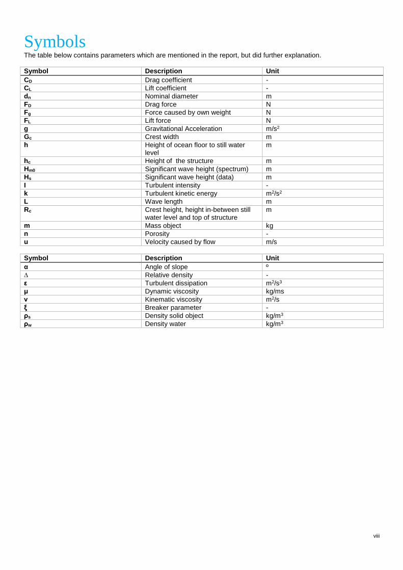
Symbols The table below contains parameters which are mentioned in the report, but did further explanation.

Symbol Description Unit

CD Drag coefficient -

CL Lift coefficient -

dn Nominal diameter m

FD Drag force N

Fg Force caused by own weight N

FL Lift force N

g Gravitational Acceleration m/s2

Gc Crest width m

h Height of ocean floor to still water level

m

hc Height of the structure m

Hm0 Significant wave height (spectrum) m

Hs Significant wave height (data) m

I Turbulent intensity -

k Turbulent kinetic energy m2/s2

L Wave length m

Rc Crest height, height in-between still water level and top of structure

m

m Mass object kg

n Porosity -

u Velocity caused by flow m/s

Symbol Description Unit

α Angle of slope º

∆ Relative density -

ε Turbulent dissipation m2/s3

μ Dynamic viscosity kg/ms

ν Kinematic viscosity m2/s

ξ Breaker parameter -

ρs Density solid object kg/m3

ρw Density water kg/m3

1

1 Introduction Delta Marine Consultants, the inventor of the Xbloc, is currently investigating the applicability of the XblocPlus. The current Xblocs are placed with a random orientation to ensure high stability and low concrete demand. However, crane operators sometimes prefer regular placement. The new XblocPlus is placed in a regular pattern, which is easier for contractors to construct and has an aesthetically smooth appearance.

Many model tests regarding the stability of the XblocPlus on a slope have already been performed, resulting in the most favourable shape of the new armour block. A detail that still needs further attention is the transition from the slope to the crest of the structure. The uniform placement of the XblocPlus elements leads to interlocking of the elements located in the middle of the slope. Since the upper element in the slope is not supported by an element located above it, the element mainly obtains its stability from its own weight, leading to a lower resistance against wave impact. Until now, several ideas for the optimal transition have been developed, but the optimal design is yet to be confirmed. This report focusses on parameters which provide the stability of the upper element.

1.1 Objective The main objective of the thesis is to find the optimal transition from the slope to the crest of a breakwater when applying a XblocPlus armour layer. The main research question is for that reason defined as:

Which crest transition of an XblocPlus armour layer is the most promising? Most promising is defined as the specific solution which is the most stable under design wave conditions, which can be constructed with the least required changes to the current element. To understand the failure of the upper element, information on the physical processes leading to failure of the element is required. The first sub-question is defined as:

Which physical parameters influence the stability of the upper element of an XblocPlus armour layer?

1.2 Approach To answer all of the above mentioned questions, the thesis is separated in three different phases. The first phase mainly focusses on understanding the failure of the upper element. The second phase focusses on modeling the failure using numerical model tests. The last phase tries to describe in which way the crest detail can be modified to increase its resistance as much as possible.

1.2.1 Understanding the process

The main goal of the first phase is to understand the physical parameters leading to failure of the upper element. By applying physical model tests, the failure of the element can be visually observed. During the physical model tests several breakwater configurations are tested where the upper element is not supported by any material behind or on top of it. These test are performed using several relative crest heights. The data obtained during the physical model tests are used as input for the further phases in the process.

1.2.2 Model the process

If the physical phenomena which leads to failure of the upper element are known, the situation will be reconstructed using a computational fluid dynamic (CFD) model in OpenFoam. OpenFoam is able to solve the Reynolds averaged Navier Stokes equations and apply a volume of fluid approach (VOF) for multi-phase flows. The biggest advantage of OpenFoam is the possibility to model turbulent flows around 3D objects. Thereby, the program is open-source, which means that it can be used without any fees. OpenFoam is applied for two different models, a 2D porous wave model simulating the physical model tests and a 3D single phase model simulating the flow around a single XblocPlus unit. The main purpose of the 2D model of the wave flume is to qualitatively determine the pressure distribution on the upper element under wave load. The obtained data from the physical laboratory tests are applied to validate the outcome of the model. The main purpose of the 3D single phase model is to determine the drag and the lift forces around a single element. The outcome of this model will be validated using fall tests. The result of this phase is a numerical model, which is able to determine all of the loads on the upper element during the most unfavorable load combination, in the form of a factor of safety. This scenario can be compared with the results of the physical model tests to get an insight in the accuracy of the numerical model.

2

1.2.3 Avoid the process

The last phase uses the input from both the first and second phase. Based on the physical processes leading to failure as found in phase one and the results of the numerical model as generated in phase two, modifications to the crest transition are proposed. Based on new stability analysis, the increment in stability can be estimated, from which the most promising crest transition can be determined.

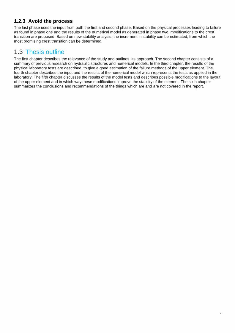
1.3 Thesis outline The first chapter describes the relevance of the study and outlines its approach. The second chapter consists of a summary of previous research on hydraulic structures and numerical models. In the third chapter, the results of the physical laboratory tests are described, to give a good estimation of the failure methods of the upper element. The fourth chapter describes the input and the results of the numerical model which represents the tests as applied in the laboratory. The fifth chapter discusses the results of the model tests and describes possible modifications to the layout of the upper element and in which way these modifications improve the stability of the element. The sixth chapter summarizes the conclusions and recommendations of the things which are and are not covered in the report.

3

2 Literature 2.1 Introduction This chapter describes a summary of the literature research done to get an indication of the physical phenomena which play a role in the design of a breakwater crest. For that reason overtopping, stability and overtopping are outlined in most detail.

2.1.1 Dimensions breakwater

The design formulae, show several different parameters. This paragraph describes the dimensions indicating the dimensions of a breakwater and several dimensionless numbers. In Figure 1, several dimensions of a breakwater are indicated, with: Rc Crest height, height in-between still water level and top of structure. hc Structure height, height from the ocean floor to the top of the breakwater. h Height from the ocean floor to still water level. Gc Width of the crest.

Figure 1: Breakwater dimensions

The relative density, the density of the rock in relation with water.

∆=𝜌𝑠 − 𝜌𝑤𝜌𝑤

The nominal diameter, dn, is the diameter when considering that a rock or concrete element is casted in a cube. The

definition for dn is √𝑀

𝜌

3. When applying rock, the dn50 is often applied, indicating the nominal median diameter of the

gradation based for the median weight of the gradation.

2.2 History Humans are protecting their property against the water for ages. People used to construct such revetments or breakwaters using common knowledge based on previous experiences with the forces of nature. To increase the reliability of the coastal structures, design guidelines are developed. Many available formulae in the world of coastal structures are developed using empirical fitting of laboratory data, rather than mathematical deviation. Empirical fitting is needed since the wave structure interaction is quite complex due to e.g. small scale phenomena as turbulence, non-linear behaviour of both the load and the resistance and statistical uncertainties (irregular wave attack and randomly placed units). Therefore, it is still quite common to first design a coastal structure based on the available guidelines where after the design is verified with the use of a physical model. Numerical models, representing the wave structure interaction, are becoming more accurate all the time, but these models still need some time to develop. Especially in cases with innovative construction materials, model tests still need to be applied to verify the different design parameters.

4

2.2.1 Rock

Natural rock or riprap is a commonly used material for breakwaters and revetments. Advantages of a riprap breakwater are the flexibility and the relative density of the rock. Disadvantages are the availability at some project locations and the limitation in size. Rock is a natural product, that has to be mined in quarries, often with the use of explosions, leading to fractionized rock. If the required rock size becomes too high, quarrying the rock becomes very difficult, leading to enormous costs or unavailability of the required material. In these cases it may be a right decision to apply concrete armour units. Many cases still require rock as a filter layer or the core of the structure.

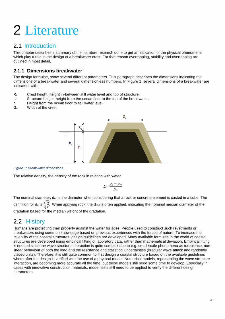
2.2.2 Concrete armour units Concrete armour units can be grouped in several clusters, based on the method of placement and the way of achieving stability. Concrete armour units can be placed randomly or uniformly, both in a single or a double layer configuration. A disadvantage of a double layered concrete armour is the concrete demand. While constructing a single layer of armour units requires a high safety factor, since the failure of a single block can lead to total breakwater failure. The stability can either be achieved by friction, interlocking or weight (see section 2.4). In Figure 2 an overview of commonly used block can be found. Recently, the cube is also used as an uniformly placed single layered armour layer (see section 2.7.2).

Figure 2: Overview concrete elements (Reedijk, 2017)

2.2.3 XblocPlus The XblocPlus is a concrete armour element, which is placed in a regular pattern. Many tests regarding the stability of the XblocPlus on a slope have already been performed, resulting in the most favourable shape of the new armour block. In Table 1, typical dimensions for the XblocPlus are indicated and in Figure 3 an artistic impression of the block is shown. The armour unit is designed in such a way that the block is completely horizontal under a slope of 35.3º. This indicates that the blocks are slightly orientated backward on a 2:3 slope and slightly forward under a 3:4 slope. Table 1: Typical dimensions XblocPlus

Value

Width block D [m] D

Length block L [m] 1.27 D

Height block H [m] 0.50 D

5

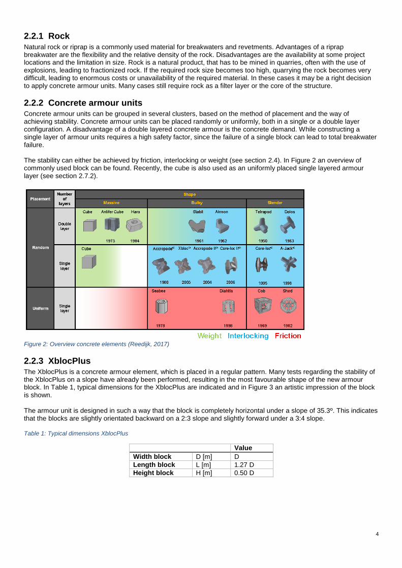
Figure 3: Artistic impression XblocPlus

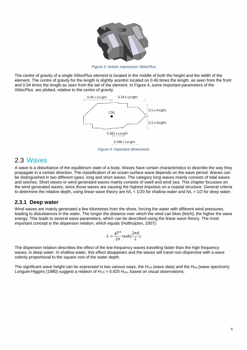
The centre of gravity of a single XblocPlus element is located in the middle of both the height and the width of the element. The centre of gravity for the length is slightly acentric located on 0.46 times the length as seen from the front and 0.54 times the length as seen from the tail of the element. In Figure 4, some important parameters of the XblocPlus are plotted, relative to the centre of gravity.

Figure 4: Important dimensions

2.3 Waves A wave is a disturbance of the equilibrium state of a body. Waves have certain characteristics to describe the way they propagate in a certain direction. The classification of an ocean surface wave depends on the wave period. Waves can be distinguished in two different types, long and short waves. The category long-waves mainly consists of tidal waves and seiches. Short waves or wind generated waves mainly consists of swell and wind sea. This chapter focusses on the wind generated waves, since those waves are causing the highest impulses on a coastal structure. General criteria to determine the relative depth, using linear wave theory are h/L < 1/20 for shallow water and h/L > 1/2 for deep water.

2.3.1 Deep water

Wind waves are mainly generated a few kilometres from the shore, forcing the water with different wind pressures, leading to disturbances in the water. The longer the distance over which the wind can blow (fetch), the higher the wave energy. This leads to several wave parameters, which can be described using the linear wave theory. The most important concept is the dispersion relation, which equals (Holthuijzen, 2007):

𝐿 =𝑔𝑇2

2𝜋tanh(

2𝜋𝑑

𝐿)

The dispersion relation describes the effect of the low-frequency waves travelling faster than the high frequency waves, in deep water. In shallow water, this effect disappears and the waves will travel non-dispersive with a wave celerity proportional to the square root of the water depth. The significant wave height can be expressed in two various ways, the H1/3 (wave data) and the Hmo (wave spectrum). Longuet-Higgins (1980) suggest a relation of H1/3 = 0.925 Hmo, based on visual observations.

6

2.3.2 Shallow water

In shallow water, waves will start to shoal (increase in wave height) and eventually break. According to the dispersion relation, the wave speed in shallow waters will go down. Waves will break if the wave steepness becomes too high or if the water becomes too shallow. The wave steepness is defined as the height of the wave divided by the length of the wave (H/L). The breaking criterion by Miche states that the breaking wave height, on a horizontal bottom, equals (Schiereck, 2016):

𝐻𝑏 = 0.142𝐿 tanh(2𝜋

𝐿ℎ)

For deep water waves, this criterion shows a maximum wave steepness of breaking of 0.14, while in practice a steepness higher than 0.05 is seldom seen (Schiereck, 2016). In shallow water, the water depth often becomes of more importance than the wave length. As stated in Holthuijzen (2007) many different values of the breaker parameter γ (Hmax/(d+η)) have been observed. On average one can find an average value of 0.88 when applying the Miche criterion while Kaminsky and Kraus (1993) found a range of values in-between 0.6 to 1.59 with an average of 0.78. Due to this high spread in values, statistics should be involved to estimate the effect of wave breaking. The breaker parameter describes the maximum wave height which can exist without breaking. Battjes and Janssen (1978) found that the fraction of the total broken waves (Qb) is Rayleigh distributed and described as:

1 − 𝑄𝑏ln(𝑄𝑏)

= −(𝐻𝑟𝑚𝑠

𝐻𝑚

)2

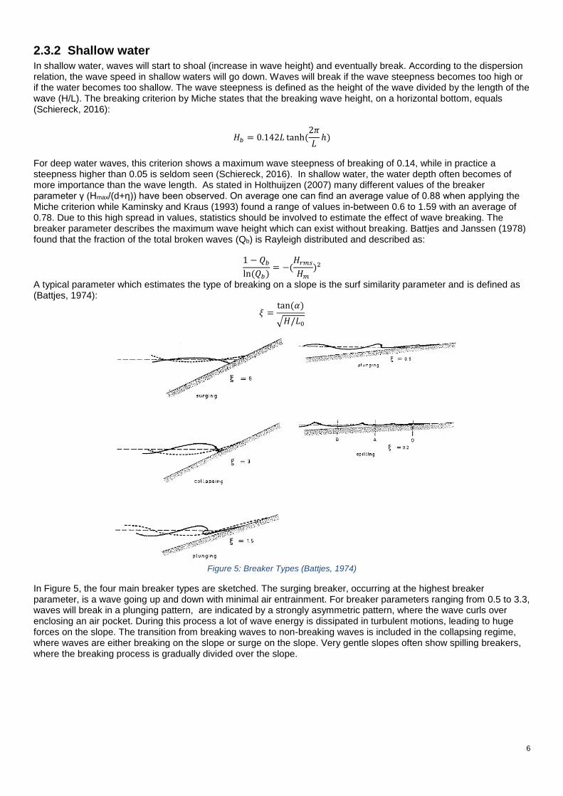
A typical parameter which estimates the type of breaking on a slope is the surf similarity parameter and is defined as (Battjes, 1974):

𝜉 =tan(𝛼)

√𝐻/𝐿0

Figure 5: Breaker Types (Battjes, 1974)

In Figure 5, the four main breaker types are sketched. The surging breaker, occurring at the highest breaker parameter, is a wave going up and down with minimal air entrainment. For breaker parameters ranging from 0.5 to 3.3, waves will break in a plunging pattern, are indicated by a strongly asymmetric pattern, where the wave curls over enclosing an air pocket. During this process a lot of wave energy is dissipated in turbulent motions, leading to huge forces on the slope. The transition from breaking waves to non-breaking waves is included in the collapsing regime, where waves are either breaking on the slope or surge on the slope. Very gentle slopes often show spilling breakers, where the breaking process is gradually divided over the slope.

7

2.3.3 Reflection

The steeper the slope, the more wave energy will be reflected, indicating that less energy is absorbed by the slope. Reflection is especially important in harbour basins, leading to higher surface elevations than normal. One should also account for reflection when performing physical model tests, since the reflected wave energy will superimpose with the incoming wave height, which leads to irregularities in the measurements. It is possible to measure the reflected wave using a three probe measuring system as initiated by Mansard and Funke (1980). The method applies the fact that a wave signal, consisting of an infinite amount of elements where each can be described with their own frequency, amplitude and phase, travelling with their own celerity. Both the incoming and the reflected wave have their own properties. Since the distance in-between probes and the distance from probe to structure are known, one is able to follow the different wave elements in time and space. The reflected wave can be excluded from the measured values subtracting the reflected wave train from the measured values, resulting in the incoming wave parameters. In theory, this analysis can be performed using two wave probes, however when applying two probes the accuracy of the measurements may reduce, due to e.g. critical wave lengths and non-linear behaviour.

2.3.4 Swash If a wave breaks on a slope, some water will still run-up on the slope with a certain velocity. The small layer of water oscillating on the slope is called swash. The EurOtop manual (2016) summarizes several researches which empirically determined the maximum wave run-up and the run-up velocity distribution on a slope of coastal dikes, which are often characterized by smooth slopes. The mean value of the maximum wave run-up of armoured slopes can be estimated by:

𝑅𝑢2%𝐻𝑚0

= 1.65𝛶𝑏𝛶𝑓𝛶𝛽𝜉𝑚−1,0

With a maximum of: 𝑅𝑢2%𝐻𝑚0

= 1.00𝛶𝑓𝑠𝑢𝑟𝑔𝑖𝑛𝑔𝛶𝛽(4.0 −1.5

√𝛶𝑏𝜉𝑚−1,0

)

The standard deviation of the first formula is 0.10 while the standard deviation for the maximum equals 0.07. The γ values are reduction factors, depending on the properties of the slope (see 2.5.2). The maximum run-up velocity can be determined using:

𝑣𝐴,2% = 𝑐𝑣2%(𝑔(𝑅𝑢2% − 𝑧𝐴))0.5

Where 𝑐𝑣2% is a coefficient, which is approximately 1.4-1.5 for slopes between 1:3 and 1:6 and zA the vertical distance

in-between the mean water level and the location on the slope where the run-up velocity is determined. It should be noted that the above equation is determined using physical model tests on an impermeable smooth grass slope, while the equation for run-up is specified for rubble or concrete element breakwaters. Next to that, the maximum flow velocity formula is based on relative shallow slopes with a range of 1:3 to 1:6. For steeper slopes, one has to extrapolate the obtained values, leading to extra uncertainties. The above relations can for that reason be applied on the slope, only to express the flow velocity in a certain order of magnitude.

2.3.5 Spectra A wave spectrum describes how the variance of the sea-surface is distributed over the frequencies. For a fully developed spectrum in deep water, the Pierson-Moskowitz (PM) spectrum is often applied, however, in most cases, the fetch is limited, which does not allow the wave spectrum to fully develop. Therefore, the Joint North Sea Wave Project (JONSWAP) did derive the shape of the energy density function in deep water, based on visual observations, which serves as an idealised case (Hasselman, 1973):

𝐸𝐽𝑂𝑁𝑆𝑊𝐴𝑃(𝑓) = 𝛼𝑔2(2𝜋)−4𝑓−5exp[−5

4(

𝑓

𝑓𝑝𝑒𝑎𝑘)

−4

]𝛾exp[

−(𝑓−𝑓𝑝𝑒𝑎𝑘)2

2𝜎2𝑓𝑝𝑒𝑎𝑘2 ]

During the JONSWAP experiment, a clear trend was found for several parameters, an average value of γ (ratio of the maximal spectral energy to the maximum of the corresponding PM spectrum) = 3.3, σa = 0.07 (f ≤ fpeak) and σb = 0.09 (f ≥ fpeak)(left or right sided with of the spectral peak). For the value of α, the Pierson-Moskowitz spectrum suggests a value of 0.0081.

8

2.4 Design phenomena

2.4.1 Stability The stability of an armour layer of a breakwater, is mainly governed by three different physical parameters, the weight of the block itself, the friction in-between the blocks and the interlocking of the blocks. The load on a single grain is divided into external forces caused by the waves and internal forces caused by the seepage through the grains of the structure.

2.4.2 Stability single units

The resistance of a single grain on a slope is mainly governed by the gravitational force on the grain, which equals (ρs-ρw)gd3 for submerged grains and ρsgd3 for emerged grains (Schiereck, 2016), the resistance may decrease due to gravity of the grains on a slope with the factor: tan(Φ)cos(α)± sin(α). Where Φ is the angle of repose and α the angle of the slope. The external load consists of the drag force, the shear force and the lift force on the grain. The various forces on a grain in uniform flow can be expressed as stated by (Schiereck 2016):

𝐷𝑟𝑎𝑔𝐹𝑜𝑟𝑐𝑒:𝐹𝐷 =1

2𝐶𝐷𝜌𝑤𝑢

2𝐴𝐷

𝐿𝑖𝑓𝑡𝐹𝑟𝑜𝑐𝑒:𝐹𝐿 =1

2𝐶𝐿𝜌𝑤𝑢

2𝐴𝐿

The areas AD and AL are officially defined as the area on which the total drag or total lift force is exerted. Where AD is the area in the plane perpendicular to the flow direction and AL the area of the object in the vertical direction as seen from the incoming flow. Since the area which is under the direct load of the flow is quite hard to determine, one often implements the nominal diameter (dn

2) as an good estimator for the area.bIn Figure 6, the forces on an armour layer are schematized, where the left image indicates down rushing and the right one up rushing of the waves.

Figure 6: Forces on an armour stone (Hald, 1998)

Most of the literature refers to the stability number, which describes the relation between the load on and the strength of the structure. For breakwaters under wave load, this stability number is defined as shown below (Schierieck, 2016), which is a division of the load and the resistance mentioned above:

𝑁 =𝐻𝑠

∆𝐷𝑛

The internal flow within the breakwater does result in internal forces due to pressure differences caused by the oscillating wave motions. An important parameter for checking the importance of the pressure gradients in a structure is the leakage length. The leakage length relates the permeability and thickness of the armour layer with the parameters for the filter layer. The higher the leakage length, the harder it is for the internal structure to adjust to the external load, the more the internal load becomes normative. The leakage length is defined as (Schiereck 2016):

𝛬 = √𝑘𝐹𝑑𝐹𝑑𝑇𝑘𝑇

Mora (2017) did propose a leakage length of 4.66 m for a XblocPlus armour layer with a narrow graded filter layer. From this value it can be concluded that the head differences in the structure leads to severe internal forces. In Figure 7, a schematic figure of the internal forces in a breakwater is shown.

9

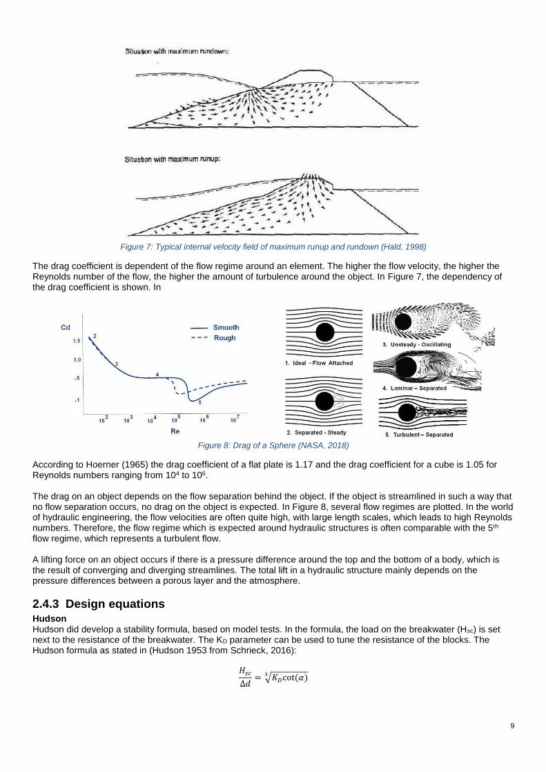
Figure 7: Typical internal velocity field of maximum runup and rundown (Hald, 1998)

The drag coefficient is dependent of the flow regime around an element. The higher the flow velocity, the higher the Reynolds number of the flow, the higher the amount of turbulence around the object. In Figure 7, the dependency of the drag coefficient is shown. In

Figure 8: Drag of a Sphere (NASA, 2018)

According to Hoerner (1965) the drag coefficient of a flat plate is 1.17 and the drag coefficient for a cube is 1.05 for Reynolds numbers ranging from 104 to 106. The drag on an object depends on the flow separation behind the object. If the object is streamlined in such a way that no flow separation occurs, no drag on the object is expected. In Figure 8, several flow regimes are plotted. In the world of hydraulic engineering, the flow velocities are often quite high, with large length scales, which leads to high Reynolds numbers. Therefore, the flow regime which is expected around hydraulic structures is often comparable with the 5th flow regime, which represents a turbulent flow. A lifting force on an object occurs if there is a pressure difference around the top and the bottom of a body, which is the result of converging and diverging streamlines. The total lift in a hydraulic structure mainly depends on the pressure differences between a porous layer and the atmosphere.

2.4.3 Design equations Hudson Hudson did develop a stability formula, based on model tests. In the formula, the load on the breakwater (Hsc) is set next to the resistance of the breakwater. The KD parameter can be used to tune the resistance of the blocks. The Hudson formula as stated in (Hudson 1953 from Schrieck, 2016):

𝐻𝑠𝑐

∆𝑑= √𝐾𝐷cot(𝛼)

3

10

Van der Meer

For slope stability, van der Meer (1988) proposed another equation for the calculation of the required stone diameters, including more different parameters which were not mentioned in the Hudson formula. Based on empirical fitting of laboratory research, the van der Meer formulae holds, including plunging and surging wave conditions:

𝑓𝑜𝑟𝜉 < 𝜉𝑡𝑟𝑎𝑛𝑠𝑖𝑡𝑖𝑜𝑛 𝐻𝑠𝑐

∆𝑑𝑛50= 6.2𝑃0.18(

𝑆

√𝑁)0.2𝜉−0.5

𝑓𝑜𝑟𝜉 > 𝜉𝑡𝑟𝑎𝑛𝑠𝑖𝑡𝑖𝑜𝑛

𝐻𝑠𝑐

∆𝑑𝑛50= 1.0𝑃−0.13(

𝑆

√𝑁)0.2𝜉𝑃√cot(𝛼)

𝜉𝑡𝑟𝑎𝑛𝑠𝑖𝑠𝑖𝑜𝑛 = [6.2𝑃0.31√tan(𝛼)](1

𝑃+0.5)

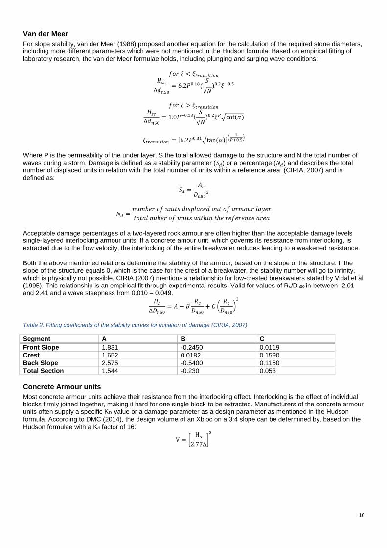
Where P is the permeability of the under layer, S the total allowed damage to the structure and N the total number of waves during a storm. Damage is defined as a stability parameter (𝑆𝑑) or a percentage (𝑁𝑑) and describes the total number of displaced units in relation with the total number of units within a reference area (CIRIA, 2007) and is defined as:

𝑆𝑑 =𝐴𝑐

𝐷𝑛502

𝑁𝑑 =𝑛𝑢𝑚𝑏𝑒𝑟𝑜𝑓𝑢𝑛𝑖𝑡𝑠𝑑𝑖𝑠𝑝𝑙𝑎𝑐𝑒𝑑𝑜𝑢𝑡𝑜𝑓𝑎𝑟𝑚𝑜𝑢𝑟𝑙𝑎𝑦𝑒𝑟

𝑡𝑜𝑡𝑎𝑙𝑛𝑢𝑏𝑒𝑟𝑜𝑓𝑢𝑛𝑖𝑡𝑠𝑤𝑖𝑡ℎ𝑖𝑛𝑡ℎ𝑒𝑟𝑒𝑓𝑒𝑟𝑒𝑛𝑐𝑒𝑎𝑟𝑒𝑎

Acceptable damage percentages of a two-layered rock armour are often higher than the acceptable damage levels single-layered interlocking armour units. If a concrete amour unit, which governs its resistance from interlocking, is extracted due to the flow velocity, the interlocking of the entire breakwater reduces leading to a weakened resistance. Both the above mentioned relations determine the stability of the armour, based on the slope of the structure. If the slope of the structure equals 0, which is the case for the crest of a breakwater, the stability number will go to infinity, which is physically not possible. CIRIA (2007) mentions a relationship for low-crested breakwaters stated by Vidal et al (1995). This relationship is an empirical fit through experimental results. Valid for values of Rc/Dn50 in-between -2.01 and 2.41 and a wave steepness from 0.010 – 0.049.

𝐻𝑠

∆𝐷𝑛50= 𝐴 + 𝐵

𝑅𝑐𝐷𝑛50

+ 𝐶 (𝑅𝑐𝐷𝑛50

)2

Table 2: Fitting coefficients of the stability curves for initiation of damage (CIRIA, 2007)

Segment A B C

Front Slope 1.831 -0.2450 0.0119

Crest 1.652 0.0182 0.1590

Back Slope 2.575 -0.5400 0.1150

Total Section 1.544 -0.230 0.053

Concrete Armour units

Most concrete armour units achieve their resistance from the interlocking effect. Interlocking is the effect of individual blocks firmly joined together, making it hard for one single block to be extracted. Manufacturers of the concrete armour units often supply a specific KD-value or a damage parameter as a design parameter as mentioned in the Hudson formula. According to DMC (2014), the design volume of an Xbloc on a 3:4 slope can be determined by, based on the Hudson formulae with a Kd factor of 16:

V = [Hs

2.77∆]3

11

In Table 3, several stability and damage parameters for different armour units are listed. Table 3: Typical damage parameters

Rock XblocPlus,v2 XblocPlus,v3 Cube (single layer)

Source CIRIA (2007) Mora (2017) Berg (2018) van Gent (2013)

Hs/∆D Nod Hs/∆D Nod Hs/∆D Hs/∆D Nod

Start of damage 1 2 2.5 >0 >4 2 >0

Failure 4 8 3.15 >0.5 3 0.2

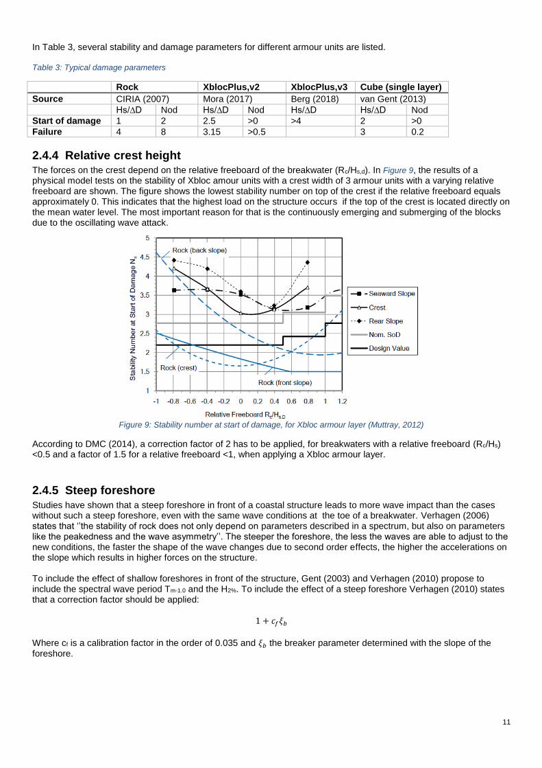
2.4.4 Relative crest height The forces on the crest depend on the relative freeboard of the breakwater (Rc/Hs,d). In Figure 9, the results of a physical model tests on the stability of Xbloc amour units with a crest width of 3 armour units with a varying relative freeboard are shown. The figure shows the lowest stability number on top of the crest if the relative freeboard equals approximately 0. This indicates that the highest load on the structure occurs if the top of the crest is located directly on the mean water level. The most important reason for that is the continuously emerging and submerging of the blocks due to the oscillating wave attack.

Figure 9: Stability number at start of damage, for Xbloc armour layer (Muttray, 2012)

According to DMC (2014), a correction factor of 2 has to be applied, for breakwaters with a relative freeboard (Rc/Hs) <0.5 and a factor of 1.5 for a relative freeboard <1, when applying a Xbloc armour layer.

2.4.5 Steep foreshore

Studies have shown that a steep foreshore in front of a coastal structure leads to more wave impact than the cases without such a steep foreshore, even with the same wave conditions at the toe of a breakwater. Verhagen (2006) states that ‘’the stability of rock does not only depend on parameters described in a spectrum, but also on parameters like the peakedness and the wave asymmetry’’. The steeper the foreshore, the less the waves are able to adjust to the new conditions, the faster the shape of the wave changes due to second order effects, the higher the accelerations on the slope which results in higher forces on the structure. To include the effect of shallow foreshores in front of the structure, Gent (2003) and Verhagen (2010) propose to include the spectral wave period Tm-1.0 and the H2%. To include the effect of a steep foreshore Verhagen (2010) states that a correction factor should be applied:

1 + 𝑐𝑓𝜉𝑏

Where cf is a calibration factor in the order of 0.035 and 𝜉𝑏 the breaker parameter determined with the slope of the foreshore.

12

2.4.6 Overtopping

Overtopping is an amount of water flowing over a sea defence (e.g. a breakwater). The overtopping over a breakwater is most of the times expressed in the total overtopping discharge (q in l/s per m). The total overtopping discharge q can be determined using (EurOtop 2016):

𝑞

√𝑔𝐻𝑚03

=0.023

√tan(∝)𝛾𝑏𝜉𝑚−1.0exp[− (2.7

𝑅𝑐𝜉𝑚−1.0𝐻𝑚0𝛾𝑏𝛾𝑓𝛾𝛽𝛾𝑣

)

1.3

]

With a maximum of:

𝑞

√𝑔𝐻𝑚03

= 0.09exp[−(1.5𝑅𝑐

𝐻𝑚0𝛾𝑓𝛾𝛽𝛾𝑣)

1.3

]

One can see that the total overtopping discharge q is dependant on the incoming spectral wave height (Hmo), the slope of the crest (α), the crest height (Rc), the breaker parameter (𝜉𝑚−1.0 see 0) and several reduction factors depending on the berm (γb), the incident wave height (γβ), a vertical structure on top of the breakwater (γv) and the permeability of the structure (γf). Since the above mentioned formulas are fitted empirically, based on many physical laboratory tests, these equations come with a certain inaccuracy. EurOtop recommends to increase the average discharge by one standard deviation to increase the reliability of the overtopping formulas. The reduction factor for permeability, mentioned in the overtopping formula, is based on the ability of the armour layer to reduce wave energy within the pores of the material. The higher the permeability, the more energy will be dissipated in the slope reducing the total overtopping discharge. Moreno (2017), proposed a roughness coefficient of 0.45 when using a XblocPlus amour layer on a 3:4 slope. The tests have been performed with a crest width of 3 Dn. The crest was made of rubble mound during the tests. Table 4 shows several permeability factors, as stated by Bruce (2007). Table 4: Typical roughness values (Bruce, 2007)

Type of Armour γf

Smooth 1.00

Rock (two layer; permeable core) 0.40

Xbloc 0.45

Accropode 0.46

Single layer Cube 0.50

The width of the crest height decreases the overtopping discharge as well, the reduction factor equals (Besley, 1999), based on tests with a rock armour layer and a permeable core:

𝐶𝑟 = 3.06exp(−1.5𝐺𝑐𝐻𝑚0

)

The equation does not include the effect of the permeability of the crest. When Gc/Hmo < 0.75, one may assume that Cr equals one. The wider the crest height of the breakwater, the more the overtopping wave height will be reduced, since the water will be absorbed by the crest. According to Verhagen (2004) it is economically not attractive to try to lower the crest by making the crest wider.

2.4.7 Transmission

If the relative crest height becomes too low, not all of the wave energy in the cross section of the breakwater gets absorbed by the structure anymore, leading to wave formations behind the breakwater (not considering wave diffraction and wave reflection at the lee side of the breakwater). In these cases, the total reduction in wave energy becomes important.

13

2.5 Laboratory work Testing a design in the wave flume requires scaling to make sure that the conditions in the flume are comparable to the conditions in the real world. If the parameters are not scaled correctly, one may misinterpret the obtained result, leading to a misinterpretation of the real conditions. According to Hughes (1993), ‘’mayor flow problems can be simplified into two major forces dominate and the other forces are minor’’. Most of the times, the inertia force needs to be balanced by another force. The inertia force can for example be balanced by gravity force (Froude criterion) or the viscous force (Reynolds criterion). Scaling the Reynolds number is not required if the Reynolds number is higher than 3*104 (Dai, 1969). If the number exceeds this certain threshold, no trends between the scaled and the unscaled structures could be spotted. The Froude number is defined as:

𝐹𝑟 =𝑢

√𝑔ℎ

If the Froude number in the laboratory is equal to the Froude number in real life, one can state that the Froude criterion is fulfilled. If the non-dimensional parameters are equal, one can state that the relation of the inertial forces and the weight of the particles are the same (Hughes, 1993). Other parameters which should exceed a certain value to represent the real situation properly (EurOtop, 2016); Water depth should be much larger than 2.0 cm Wave periods should be larger than 0.35 s Wave heights should be larger than 5.0 cm (Weber Criterion) To avoid the effects of surface tension.

2.5.1 Stability

The stability measured in the laboratory can be compared with the real stability by applying the stability number. The stability numbers (Hs/(∆Dn50)) should be equal to each other (CIRIA, 2007). When equalizing the stability numbers one also automatically takes care of density differences. The water on the project location is often salty, while the water in the flume is fresh most of the time.

2.5.2 Overtopping

The overtopping can be scaled by applying the dimensionless overtopping discharge (q/(gHm03)0.5. EurOtop (2016)

states that a dimensionless overtopping limit of 10-6 is hardly exceeded and can therefore be used as a zero overtopping limit. A second scaling requirement for the overtopping calculation is the dimensionless freeboard (Rc/Hs) , which can also be scaled to real life projects.

2.6 Crest design

2.6.1 Current guidelines

In most researches and guidelines, the current minimum required crest width is based on the relative freeboard of the breakwater (freeboard/wave height). In Table 5, several recommended values for different armour units are shown. The minimum required crest width is mainly determined by the construction method. If one choses for a land based method, cranes and trucks should be able to travel over the crest, leading to a higher required crest width. CIRIA(2007) states that a minimum of three rows is required for safe placement and to ensure sufficient interlocking for concrete armour units. For the above mentioned practical reasons, most of the overtopping relations are based on the application of three armour stones on top of the crest.

Table 5: Minimum required crest width

Rock Xbloc

Source CIRIA (2007) DMC (2014)

Emerged 3 – 4 Dn50 2.28 D

Crown wall 3 – 4 Dn50 1.64 D

14

Figure 10: Burj Al Arab breakwater (Ingber, 2018)

2.6.2 Crest height

As a rule of thumb, the relative crest height for coastal structures is often 0.8 to 1 for breakwaters and 1.2 to 1.4 for revetments, based on practical knowledge. These values are often resulting from the overtopping requirements, which are often more strict for revetments, which are protecting valuable property. For the design of breakwaters, surrounded by sea at both sides of the cross section, these requirements are often lower.

2.6.3 Constructability

The constructability of a structure can be defined as: ‘’ Degree to which the integration of experience and knowledge in a construction process facilitates achievement of an optimum balance between project goals and resource constraints’’ (BuisnessDictionary, 2018). One can state that constructing in dry circumstances is easier than constructing in wet circumstances, since the visibility of the work is better above the still water level than below the still water level. For logistical reasons it is better to have as few as possible different materials and material sizes, since all of these different materials have to be stored and casted on side, which requires a lot of space, which is not always available. At last proposed solutions need to be as easy makeable and locatable as possible.

2.7 Applied crests Several breakwaters consisting of a uniformly placed single layer armour units have been constructed around the globe. Challenges for the application of these uniformly placed blocks is to try to keep the horizontal rows as horizontal as possible, to ensure there are no vertical jumps on the crest of the structure.

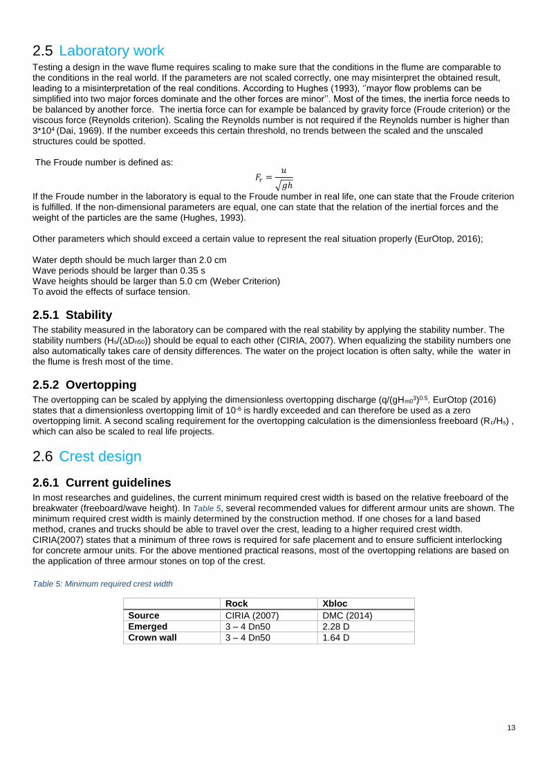
2.7.1 Burj Al Arab

The revetment Burj Al Arab consists of a single layer uniformly placed SHED block Armor layer. This revetment is part of an offshore island, on which the Burj Al Arab tower is build. Figure 10 shows an image of the revetment. One can see that the rows of SHED blocks are placed in perfect horizontal lines. In-between the revetment and the promenade (the crest of the breakwater itself) a single row of stones is placed to fill the gap. Allsop (1996) did include a typical cross section of a SHED breakwater in the design guidelines for the application of single layer hollow cube armour. To construct the SHED rows completely horizontally, a precast concrete toe berm should be applied, which increases the complexity of the construction during extreme weather conditions.

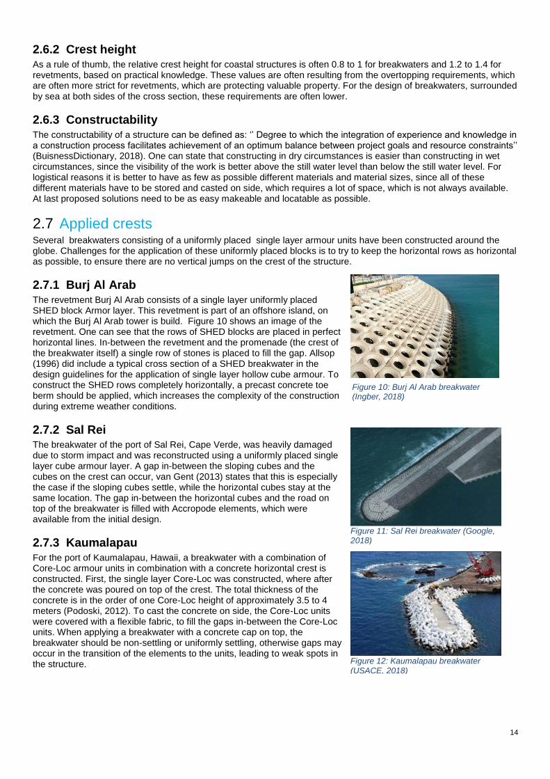
2.7.2 Sal Rei The breakwater of the port of Sal Rei, Cape Verde, was heavily damaged due to storm impact and was reconstructed using a uniformly placed single layer cube armour layer. A gap in-between the sloping cubes and the cubes on the crest can occur, van Gent (2013) states that this is especially the case if the sloping cubes settle, while the horizontal cubes stay at the same location. The gap in-between the horizontal cubes and the road on top of the breakwater is filled with Accropode elements, which were available from the initial design.

2.7.3 Kaumalapau

For the port of Kaumalapau, Hawaii, a breakwater with a combination of Core-Loc armour units in combination with a concrete horizontal crest is constructed. First, the single layer Core-Loc was constructed, where after the concrete was poured on top of the crest. The total thickness of the concrete is in the order of one Core-Loc height of approximately 3.5 to 4 meters (Podoski, 2012). To cast the concrete on side, the Core-Loc units were covered with a flexible fabric, to fill the gaps in-between the Core-Loc units. When applying a breakwater with a concrete cap on top, the breakwater should be non-settling or uniformly settling, otherwise gaps may occur in the transition of the elements to the units, leading to weak spots in the structure.

Figure 11: Sal Rei breakwater (Google, 2018)

Figure 12: Kaumalapau breakwater (USACE, 2018)

15

2.7.4 Placed block revetment

Another uniform placed revetment is the placed block revetment. To obtain the horizontal rows, a fixed toe construction is often constructed, serving as a base, on which the blocks are placed. The crest of a placed block revetment is comparable to the crest in Figure 10 or constructed in gradual arcs.

2.8 Numerical modelling

2.8.1 OpenFoam During the process, the numerical models are built in the open source computational fluid dynamics (CFD) model OpenFoam. OpenFoam is able to solve the Navier Stokes equations numerically with or without the application of a turbulence model. The version used for the models is OpenFOAM 5.0. Information regarding the boundary conditions of OpenFoam can be found in Appendix B. In addition to OpenFoam, the waves2Foam toolbox which is able to generate numerical waves according to a specified wave spectrum and generate porous layers which are able to determine the difference in pressure within a porous layer. The waves2Foam is published under Jacobsen et al. (2012) and the porosity implementation in Jensen et al. (2014).

2.8.2 Equations

Navier Stokes

The Navier Stokes equations describe the conservation laws of mass, momentum and energy. The continuity equation (conservation of mass) describes that molecules cannot disappear. The momentum equation describes the second law of Newton and notices that the force is equal to the mass times the acceleration. Conservation of energy indicates that all energy will remain in the system, either by work or by temperature increment.

Reynolds averaging

The Navier Stokes equations do include the effect of turbulence. Since the timescale for the turbulent eddies is often smaller than the timescale of the mean flow, solving the complete turbulent motion in the model will lead to a small timescale and grid scale and herewith a high computational demand. The Reynolds averaging decouples the flow velocity to a mean and a fluctuating part. The time average of the turbulent time series equals zero, which reduces the total number of elements in the equations. Applying Reynolds averaging introduces new unknown parameters in the equations, tangential stress terms and normal stress terms. To properly solve these terms, a turbulent closure model is required to make sure there is an equation available to solve each unknown term. A possible model to assume the eddy viscosity, resulting from Reynolds averaging the Navier Stokes equation, is the k-ε model. This model is quite often applied in the world of hydraulic engineering. The eddy viscosity in the model is formulated as, where C1 is an empirical coefficient often equal to 0.09 (Uijttewaal, 2018):

𝑣𝑡 = 𝐶1𝑘2

𝜀

Applying the k-ε model closure model will give results which are in the right order of magnitude. The model starts to differentiate from reality if the empirical parameters are applied for unique situations.

Volume averaging

Volume averaging is often uses to model the flow in porous media. Flow in porous media is complex since water is able to flow through the voids and will flow in all directions. Modeling all the porous flow in all the directions requires a very fine mesh, which is often not required for accuracy. To reduce the number of grid cells, the flow in the pours can be averaged to a net inflow and a net outflow in a computational cell. All cells are assigned with a value in-between 0 and 1, where a value of 0 corresponds to an empty cell and a value of 1 to a saturated cell. All values in-between 0 and 1 corresponds to a cell partly filled with water.

16

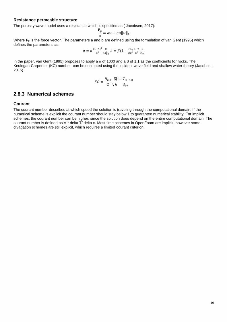
Resistance permeable structure

The porosity wave model uses a resistance which is specified as ( Jacobsen, 2017): 𝑭𝑝

𝜌= 𝑎𝒖 + 𝑏𝒖‖𝒖‖𝟐

Where Fp is the force vector. The parameters a and b are defined using the formulation of van Gent (1995) which defines the parameters as:

𝑎 = 𝛼(1−𝑛)2

𝑛3

𝜇

𝜌𝑑502 𝑏 = 𝛽(1 +

7.5

𝐾𝐶)1−𝑛

𝑛3

1

𝑑50

In the paper, van Gent (1995) proposes to apply a α of 1000 and a β of 1.1 as the coefficients for rocks. The Keulegan-Carpenter (KC) number can be estimated using the incident wave field and shallow water theory (Jacobsen, 2015).

𝐾𝐶 =𝐻𝑚0

2√𝑔

ℎ

1.1𝑇𝑚−1,0

𝑑50

2.8.3 Numerical schemes

Courant

The courant number describes at which speed the solution is traveling through the computational domain. If the numerical scheme is explicit the courant number should stay below 1 to guarantee numerical stability. For implicit schemes, the courant number can be higher, since the solution does depend on the entire computational domain. The courant number is defined as V * delta T/ delta x. Most time schemes in OpenFoam are implicit, however some divagation schemes are still explicit, which requires a limited courant criterion.

17

3 Physical model tests 3.1 Introductory lab tests The main purpose of the introductory physical model test is to gain insight in the failure methods of the upper XblocPlus element with and without any fortifications. Due to the limited available time in the wave flume, the breakwater and the foreshore were already located in the flume, which limited the available variables. Modifications to the breakwater crest were possible. The test results can be found in appendix A.

3.1.1 Lab configuration

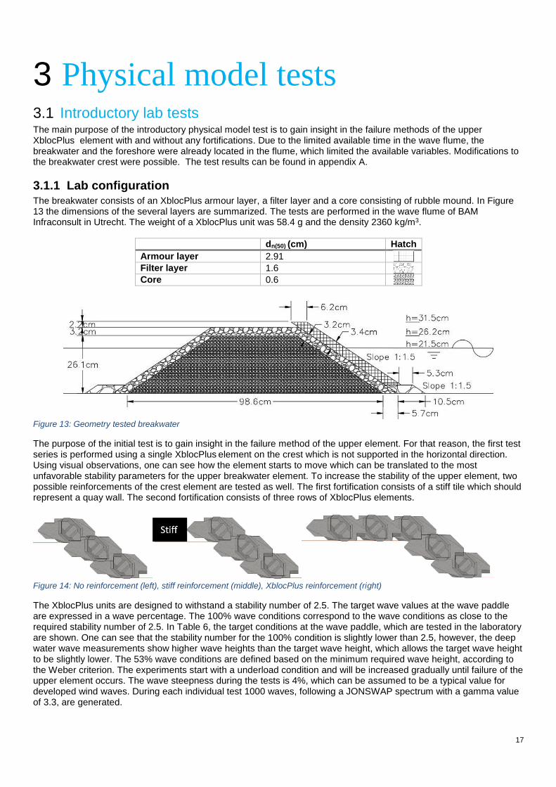
The breakwater consists of an XblocPlus armour layer, a filter layer and a core consisting of rubble mound. In Figure 13 the dimensions of the several layers are summarized. The tests are performed in the wave flume of BAM Infraconsult in Utrecht. The weight of a XblocPlus unit was 58.4 g and the density 2360 kg/m3.

dn(50) (cm) Hatch

Armour layer 2.91 Filter layer 1.6 Core 0.6

Figure 13: Geometry tested breakwater

The purpose of the initial test is to gain insight in the failure method of the upper element. For that reason, the first test series is performed using a single XblocPlus element on the crest which is not supported in the horizontal direction. Using visual observations, one can see how the element starts to move which can be translated to the most unfavorable stability parameters for the upper breakwater element. To increase the stability of the upper element, two possible reinforcements of the crest element are tested as well. The first fortification consists of a stiff tile which should represent a quay wall. The second fortification consists of three rows of XblocPlus elements.

Figure 14: No reinforcement (left), stiff reinforcement (middle), XblocPlus reinforcement (right)

The XblocPlus units are designed to withstand a stability number of 2.5. The target wave values at the wave paddle are expressed in a wave percentage. The 100% wave conditions correspond to the wave conditions as close to the required stability number of 2.5. In Table 6, the target conditions at the wave paddle, which are tested in the laboratory are shown. One can see that the stability number for the 100% condition is slightly lower than 2.5, however, the deep water wave measurements show higher wave heights than the target wave height, which allows the target wave height to be slightly lower. The 53% wave conditions are defined based on the minimum required wave height, according to the Weber criterion. The experiments start with a underload condition and will be increased gradually until failure of the upper element occurs. The wave steepness during the tests is 4%, which can be assumed to be a typical value for developed wind waves. During each individual test 1000 waves, following a JONSWAP spectrum with a gamma value of 3.3, are generated.

18

Table 6: Target wave conditions at wave paddle (deep water)

Percentage 53 60 80 100 110 120 130 140 150

Hmo/(∆dn) 1.26 1.44 1.92 2.40 2.64 2.88 3.12 3.36 3.60

Hm0 (m) 0.05 0.057 0.076 0.095 0.105 0.114 0.124 0.133 0.143

Tp (s) 0.90 0.96 1.10 1.23 1.29 1.35 1.41 1.46 1.51

A higher wave impact on the crest elements is expected if the relative crest height decreases. Therefore, the relative crest height is a variable during the tests. The relative crest height is determined using the parameters for the design wave height. To reduce the time needed until failure, the relative crest height for the fortified configurations is set to 0.5. In Table 7, the several variables during the tests is shown. Table 7: Test setups

Test series Rc/Hm0 (-) Reinforcement

1 1.0 None

2 0.5 None

3 0.0 None

4 0.5 Stiff

5 0.5 XblocPlus

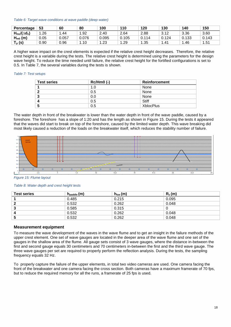
The water depth in front of the breakwater is lower than the water depth in front of the wave paddle, caused by a foreshore. The foreshore has a slope of 1:20 and has the length as shown in Figure 15. During the tests it appeared that the waves did start to break on top of the foreshore, caused by the limited water depth. This wave breaking did most likely caused a reduction of the loads on the breakwater itself, which reduces the stability number of failure.

l Figure 15: Flume layout

Table 8: Water depth and crest height tests

Test series hpaddle (m) htoe (m) Rc (m)

1 0.485 0.215 0.095

2 0.532 0.262 0.048

3 0.585 0.315 0

4 0.532 0.262 0.048

5 0.532 0.262 0.048

Measurement equipment

To measure the wave development of the waves in the wave flume and to get an insight in the failure methods of the upper crest element. One set of wave gauges are located in the deeper area of the wave flume and one set of the gauges in the shallow area of the flume. All gauge sets consist of 3 wave gauges, where the distance in-between the first and second gauge equals 30 centimeters and 70 centimeters in-between the first and the third wave gauge. The three wave gauges per set are required to properly perform the reflection analysis. During the tests, the sampling frequency equals 32 Hz. To properly capture the failure of the upper elements, in total two video cameras are used. One camera facing the front of the breakwater and one camera facing the cross section. Both cameras have a maximum framerate of 70 fps, but to reduce the required memory for all the runs, a framerate of 25 fps is used.

19

Stability elements

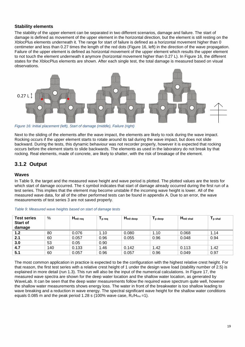
The stability of the upper element can be separated in two different scenarios, damage and failure. The start of damage is defined as movement of the upper element in the horizontal direction, but the element is still resting on the XblocPlus elements underneath it. The range for start of failure is defined as a horizontal movement higher than 0 centimeter and less than 0.27 times the length of the red dots (Figure 16, left) in the direction of the wave propagation. Failure of the upper element is defined as horizontal movement of the upper element which results the upper element to not touch the element underneath it anymore (horizontal movement higher than 0.27 L). In Figure 16, the different states for the XblocPlus elements are shown. After each single test, the total damage is measured based on visual observations.

Figure 16: Initial placement (left), Start of damage (middle), Failure (right)

Next to the sliding of the elements after the wave impact, the elements are likely to rock during the wave impact. Rocking occurs if the upper element starts to rotate around its tail during the wave impact, but does not slide backward. During the tests, this dynamic behaviour was not recorder properly, however it is expected that rocking occurs before the element starts to slide backwards. The elements as used in the laboratory do not break by that rocking. Real elements, made of concrete, are likely to shatter, with the risk of breakage of the element.

3.1.2 Output

Waves

In Table 9, the target and the measured wave height and wave period is plotted. The plotted values are the tests for which start of damage occurred. The ≤ symbol indicates that start of damage already occurred during the first run of a test series. This implies that the element may become unstable if the incoming wave height is lower. All of the measured wave data, for all of the other performed tests can be found in appendix A. Due to an error, the wave measurements of test series 3 are not saved properly. Table 9: Measured wave heights based on start of damage tests

Test series Start of damage

% Hm0 req Tp req Hm0 deep Tp deep Hm0 shal Tp shal

1.2 80 0.076 1.10 0.080 1.10 0.068 1.14

2.1 60 0.057 0.96 0.055 0.96 0.048 0.94

3.0 53 0.05 0.90

4.7 140 0.133 1.46 0.142 1.42 0.113 1.42

5.1 60 0.057 0.96 0.057 0.96 0.049 0.97

The most common application in practice is expected to be the configuration with the highest relative crest height. For that reason, the first test series with a relative crest height of 1 under the design wave load (stability number of 2.5) is explained in more detail (run 1.3). This run will also be the input of the numerical calculations. In Figure 17, the measured wave spectra are shown for the deep water location and the shallow water location, as generated by WaveLab. It can be seen that the deep water measurements follow the required wave spectrum quite well, however the shallow water measurements shows energy loss. The water in front of the breakwater is too shallow leading to wave breaking and a reduction in wave energy. The spectral significant wave height for the shallow water conditions equals 0.085 m and the peak period 1.28 s (100% wave case, Rc/Hmo =1).

20

Figure 17: Measured wave spectrum Deep water (left) and Shallow water (right), black line is required spectrum, 100% conditions

Figure 18: Theoretical wave spectrum deep water (black line) and shallow water (red line) for test series 1.3, spectral density in m2s

In Table 10, the damage parameters for the different test series are summarized. The damage percentages do correspond to the incoming deep water wave height, based on the theoretical wave spectrum. While the damage numbers corresponds to the deep and shallow water wave height respectively. The ≤ symbol indicates that start of damage already occurred during the first run of a test series. This implies that the element may become unstable if the incoming wave height is lower. The ≥ indicates that the upper element did not show any damage after the entire test series. For that reason, the stability number is as least higher than the case with the highest wave impact. m2

Table 10: Test results

Test Damage Failure

% 𝐻𝑚0

∆𝑑𝑛50 Deep

𝐻𝑚0

∆𝑑𝑛50 Shal % 𝐻𝑚0

∆𝑑𝑛50 Deep

𝐻𝑚0

∆𝑑𝑛50 Shal

1 80 2.0 1.76 None ≥ 3.75 ≥ 2.67

2 ≤60 ≤1.5 ≤ 1.24 ≤60 ≤1.5 ≤ 1.24

3 ≤53 ≤1.3 ≤53 ≤1.3

4 140 3.5 2.93 None ≥ 3.75 ≥ 3.01

5 ≤60 ≤1.5 ≤ 1.27 80 2.0 1.82

To properly estimate the up-rushing velocity on the breakwater caused by the waves on the structure. During the test under the design conditions (stability number 2.5) for a relative crest height of 1, the up-rushing velocity appeared to be in the order of 2 cm per frame, with an accuracy of +/- 0.5 cm/frame. Which is equal to a velocity of 0.5 m/s with an accuracy of +/- 0.13 m/s.

Variance Spectrum

Incident Reflected Noise/Error

Frequency [Hz]21.81.61.41.210.80.6

Sp

ectr

al D

en

sity [m

²·s]

0.0035

0.003

0.0025

0.002

0.0015

0.001

0.0005

0

Variance Spectrum

Incident Reflected Noise/Error

Frequency [Hz]

21.81.61.41.210.80.6

Spectr

al D

ensity

[m

²·s]

0.002

0.0015

0.001

0.0005

0

21

3.1.3 Notes on results

During the all of the tests, especially for the tests in the overload cases heavy wave breaking did occur on the foreshore in front of the breakwater. This heavy wave breaking did cause energy losses on the foreshore, leading to lower loads on the crest. This dissipation also leads to a difference in wave height in-between the middle of the foreshore and the toe of breakwater. Since the input wave height for the CFD model is located approximately one wave length in front of the structure (depending on the wave), the obtained data is recorded at the right location for the purposes of the CFD calculation. Secondly, the rocks of the filter layer, which are supporting the upper element have been placed in different ways. The support of the elements by the filter layer does heavily increase the stability of the element (see conceptual model). During the tests, this support was not checked properly, which leads to uncertainties of the results. The first test was quite loose, while the fourth test may be too tightly compacted.

3.1.4 Conclusions stability elements From the physical model tests it can be concluded that a single XblocPlus unit on top of the crest, not supported by anything behind it, is not able to withstand the required wave load with a stability number of 2.5, which holds for all the tested relative crest heights. After the failure of the upper row, the second highest row becomes the upper row. Which can be compared with a crest element supported by the material of the filter layer. During the 2nd test series, an overload case is tested after the failure of the upper row. During this overload situation it appeared that start of damage occurred during tests 2.4 (Hmo,deep = 0.11 m, Tp,deep = 1.33 s and Rc = 0.048 m). This may indicate that applying a rock backfill does increase the stability of the element significantly. Since there is no test performed simulating these conditions, definitive conclusions cannot be formulated. The layout with the stiff backfill appears to be very stable, able to resist the 140% wave height. This indicates that applying enough weight behind the upper element, will prevent the element for sliding backwards. It should be noted that rocking was not measured during these tests. This should be included to make sure the tail of the element will not break caused by the wave impact. This configuration appears to be interesting for further research. The reinforcement as tested in run 5 (3 rows of horizontal XblocPlus units) is not the optimal crest layout. The transition element appears to hold longer, however the elements which are forming the reinforcement start to slide backwards resulting in the same stability numbers as the situation when only applying a single row of XblocPlus units on top.

3.2 Visual failure element The initial lab tests did show several failure modes, depending on the number of dimensions considered. The failure modes are often not occurring independently of each other, however for insight in the processes itself, these failure modes will be treated separately in this chapter.

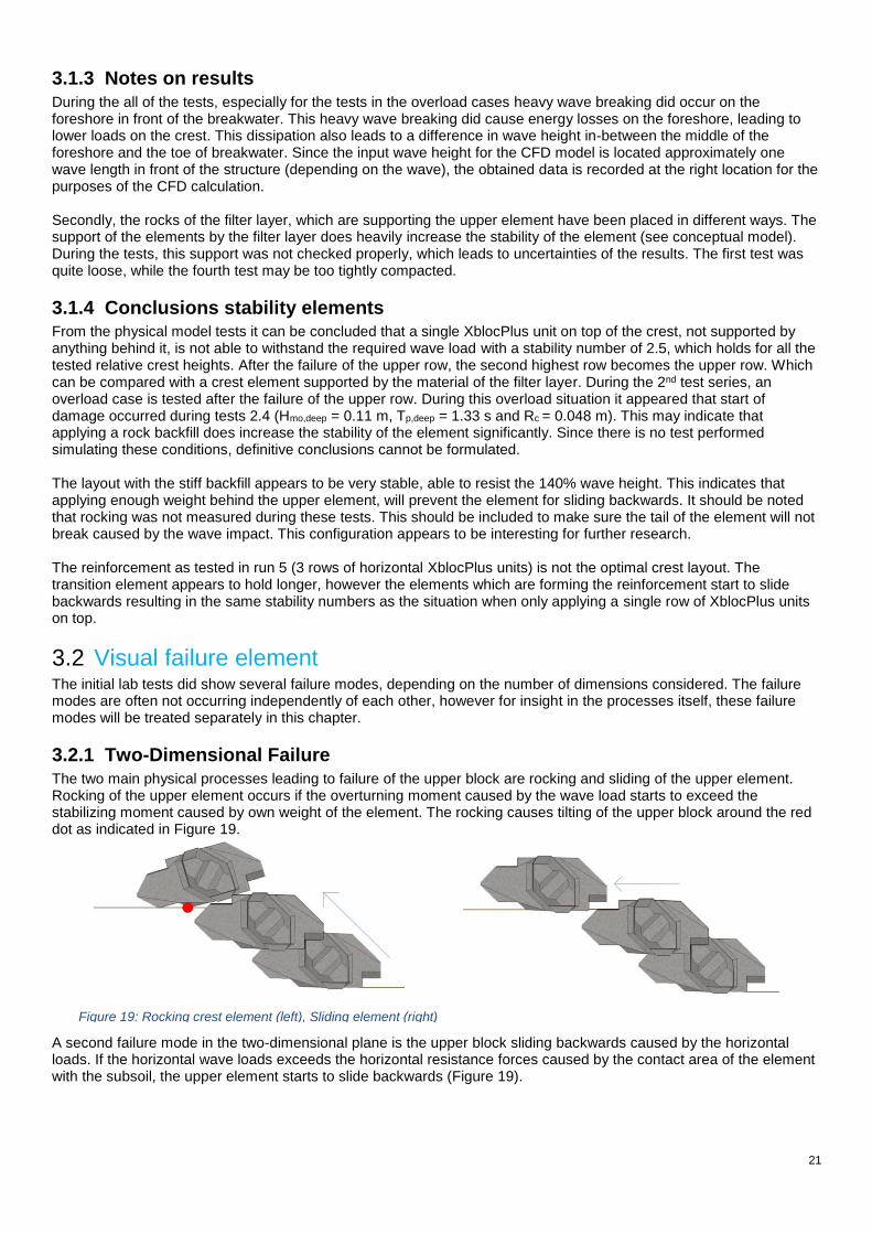
3.2.1 Two-Dimensional Failure

The two main physical processes leading to failure of the upper block are rocking and sliding of the upper element. Rocking of the upper element occurs if the overturning moment caused by the wave load starts to exceed the stabilizing moment caused by own weight of the element. The rocking causes tilting of the upper block around the red dot as indicated in Figure 19.

A second failure mode in the two-dimensional plane is the upper block sliding backwards caused by the horizontal loads. If the horizontal wave loads exceeds the horizontal resistance forces caused by the contact area of the element with the subsoil, the upper element starts to slide backwards (Figure 19).

Figure 19: Rocking crest element (left), Sliding element (right)

22

During the physical model tests, the above mentioned events did often not occur individually, but as a combination of events. In most cases the upper block first starts to rotate as indicated in Figure 19. This rocking does change the area of water impact of the upper block, since areas first covered by the concrete will be directly under the load of the water. After the wave impact, the block will fall down again on a location comparable with Figure 19. The following sub-sections hypothetically describe why the loads on a non-horizontal XblocPlus element increase. Failure for the element is defined as the element sliding backwards, where the element is not resting in its initial position anymore. Rocking of the element does not necessarily leads to failure of the element, but should be avoided to reduce the risk of breaking, caused by tension in the concrete. For that reason rocking of the element should be avoided, but data on the maximum allowed internal loads of a XblocPlus element is not available. In the study, only the external momentum equations will be considered, which allows some rocking but no sliding.

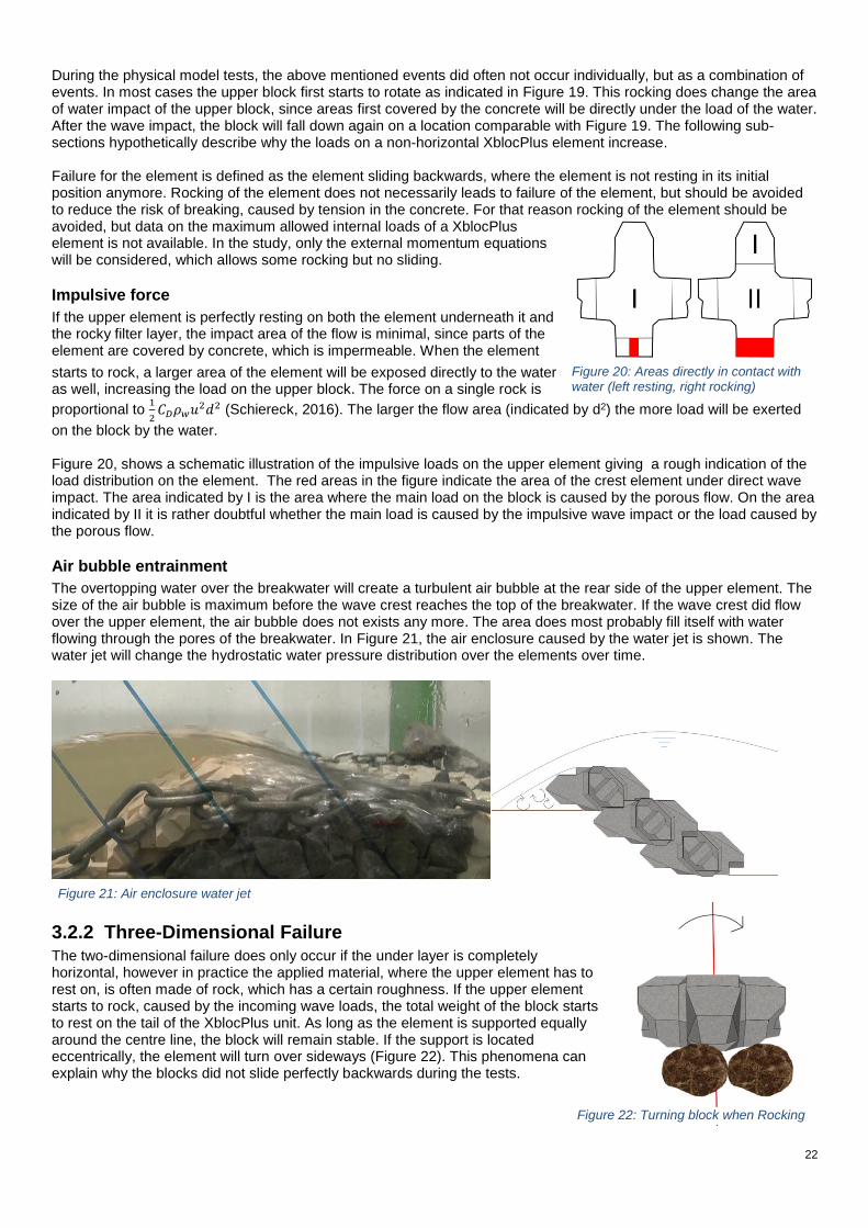
Impulsive force

If the upper element is perfectly resting on both the element underneath it and the rocky filter layer, the impact area of the flow is minimal, since parts of the element are covered by concrete, which is impermeable. When the element

starts to rock, a larger area of the element will be exposed directly to the water as well, increasing the load on the upper block. The force on a single rock is

proportional to 1

2𝐶𝐷𝜌𝑤𝑢

2𝑑2 (Schiereck, 2016). The larger the flow area (indicated by d2) the more load will be exerted

on the block by the water. Figure 20, shows a schematic illustration of the impulsive loads on the upper element giving a rough indication of the load distribution on the element. The red areas in the figure indicate the area of the crest element under direct wave impact. The area indicated by I is the area where the main load on the block is caused by the porous flow. On the area indicated by II it is rather doubtful whether the main load is caused by the impulsive wave impact or the load caused by the porous flow.

Air bubble entrainment

The overtopping water over the breakwater will create a turbulent air bubble at the rear side of the upper element. The size of the air bubble is maximum before the wave crest reaches the top of the breakwater. If the wave crest did flow over the upper element, the air bubble does not exists any more. The area does most probably fill itself with water flowing through the pores of the breakwater. In Figure 21, the air enclosure caused by the water jet is shown. The water jet will change the hydrostatic water pressure distribution over the elements over time.

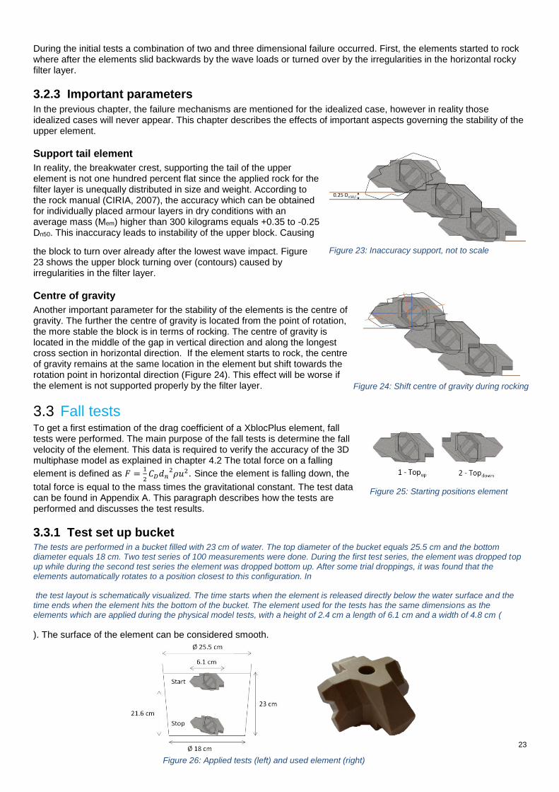
3.2.2 Three-Dimensional Failure The two-dimensional failure does only occur if the under layer is completely horizontal, however in practice the applied material, where the upper element has to rest on, is often made of rock, which has a certain roughness. If the upper element starts to rock, caused by the incoming wave loads, the total weight of the block starts to rest on the tail of the XblocPlus unit. As long as the element is supported equally around the centre line, the block will remain stable. If the support is located eccentrically, the element will turn over sideways (Figure 22). This phenomena can explain why the blocks did not slide perfectly backwards during the tests.

Figure 22: Turning block when Rocking

Figure 20: Areas directly in contact with water (left resting, right rocking)

Figure 21: Air enclosure water jet

23

During the initial tests a combination of two and three dimensional failure occurred. First, the elements started to rock where after the elements slid backwards by the wave loads or turned over by the irregularities in the horizontal rocky filter layer.

3.2.3 Important parameters In the previous chapter, the failure mechanisms are mentioned for the idealized case, however in reality those idealized cases will never appear. This chapter describes the effects of important aspects governing the stability of the upper element.

Support tail element In reality, the breakwater crest, supporting the tail of the upper element is not one hundred percent flat since the applied rock for the filter layer is unequally distributed in size and weight. According to the rock manual (CIRIA, 2007), the accuracy which can be obtained for individually placed armour layers in dry conditions with an average mass (Mem) higher than 300 kilograms equals +0.35 to -0.25 Dn50. This inaccuracy leads to instability of the upper block. Causing

the block to turn over already after the lowest wave impact. Figure 23 shows the upper block turning over (contours) caused by irregularities in the filter layer.

Centre of gravity

Another important parameter for the stability of the elements is the centre of gravity. The further the centre of gravity is located from the point of rotation, the more stable the block is in terms of rocking. The centre of gravity is located in the middle of the gap in vertical direction and along the longest cross section in horizontal direction. If the element starts to rock, the centre of gravity remains at the same location in the element but shift towards the rotation point in horizontal direction (Figure 24). This effect will be worse if the element is not supported properly by the filter layer.

3.3 Fall tests To get a first estimation of the drag coefficient of a XblocPlus element, fall tests were performed. The main purpose of the fall tests is determine the fall velocity of the element. This data is required to verify the accuracy of the 3D multiphase model as explained in chapter 4.2 The total force on a falling

element is defined as 𝐹 =1

2𝐶𝐷𝑑𝑛

2𝜌𝑢2. Since the element is falling down, the

total force is equal to the mass times the gravitational constant. The test data can be found in Appendix A. This paragraph describes how the tests are performed and discusses the test results.

3.3.1 Test set up bucket The tests are performed in a bucket filled with 23 cm of water. The top diameter of the bucket equals 25.5 cm and the bottom diameter equals 18 cm. Two test series of 100 measurements were done. During the first test series, the element was dropped top up while during the second test series the element was dropped bottom up. After some trial droppings, it was found that the elements automatically rotates to a position closest to this configuration. In

the test layout is schematically visualized. The time starts when the element is released directly below the water surface and the time ends when the element hits the bottom of the bucket. The element used for the tests has the same dimensions as the elements which are applied during the physical model tests, with a height of 2.4 cm a length of 6.1 cm and a width of 4.8 cm (

). The surface of the element can be considered smooth.

Figure 23: Inaccuracy support, not to scale

Figure 24: Shift centre of gravity during rocking

Figure 26: Applied tests (left) and used element (right)

Figure 25: Starting positions element

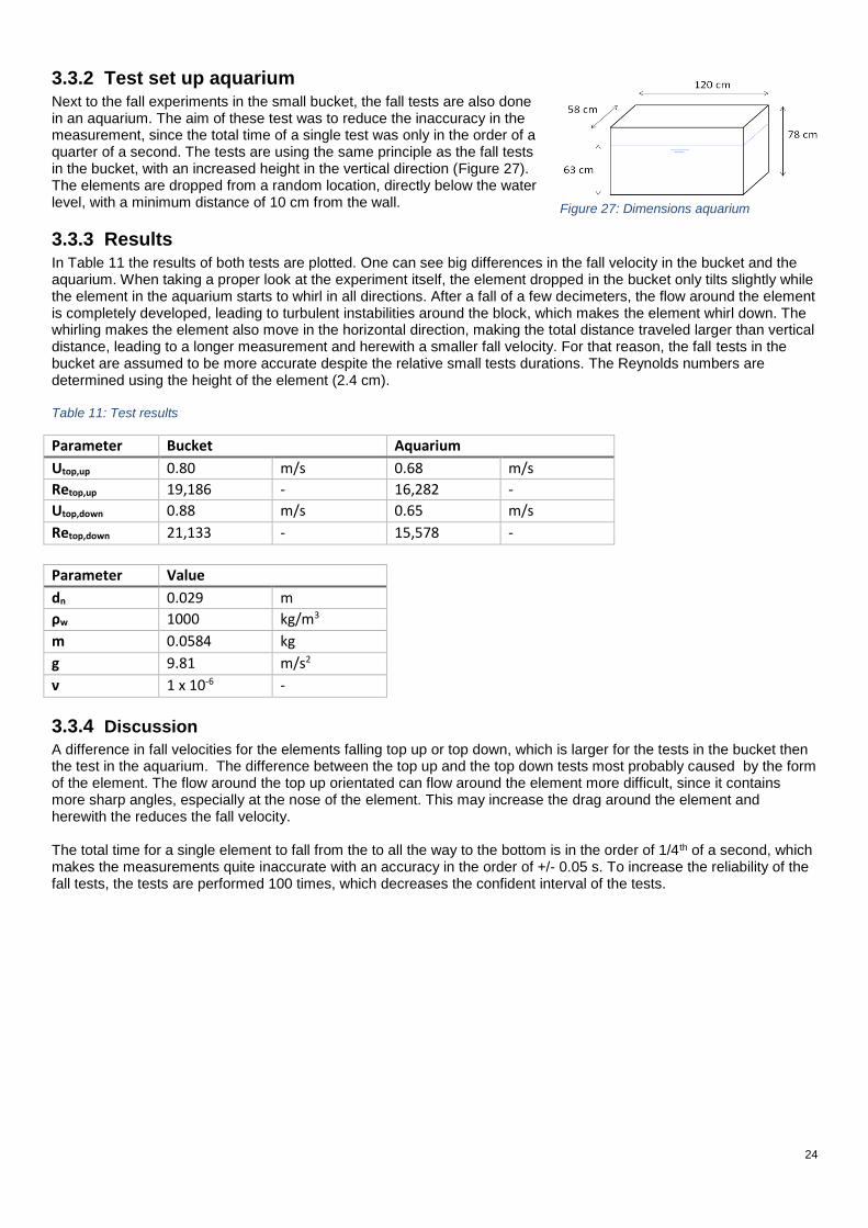
24

3.3.2 Test set up aquarium Next to the fall experiments in the small bucket, the fall tests are also done in an aquarium. The aim of these test was to reduce the inaccuracy in the measurement, since the total time of a single test was only in the order of a quarter of a second. The tests are using the same principle as the fall tests in the bucket, with an increased height in the vertical direction (Figure 27). The elements are dropped from a random location, directly below the water level, with a minimum distance of 10 cm from the wall.

3.3.3 Results In Table 11 the results of both tests are plotted. One can see big differences in the fall velocity in the bucket and the aquarium. When taking a proper look at the experiment itself, the element dropped in the bucket only tilts slightly while the element in the aquarium starts to whirl in all directions. After a fall of a few decimeters, the flow around the element is completely developed, leading to turbulent instabilities around the block, which makes the element whirl down. The whirling makes the element also move in the horizontal direction, making the total distance traveled larger than vertical distance, leading to a longer measurement and herewith a smaller fall velocity. For that reason, the fall tests in the bucket are assumed to be more accurate despite the relative small tests durations. The Reynolds numbers are determined using the height of the element (2.4 cm). Table 11: Test results

Parameter Bucket Aquarium

Utop,up 0.80 m/s 0.68 m/s

Retop,up 19,186 - 16,282 -

Utop,down 0.88 m/s 0.65 m/s

Retop,down 21,133 - 15,578 -

Parameter Value

dn 0.029 m

ρw 1000 kg/m3

m 0.0584 kg

g 9.81 m/s2

ν 1 x 10-6 -

3.3.4 Discussion

A difference in fall velocities for the elements falling top up or top down, which is larger for the tests in the bucket then the test in the aquarium. The difference between the top up and the top down tests most probably caused by the form of the element. The flow around the top up orientated can flow around the element more difficult, since it contains more sharp angles, especially at the nose of the element. This may increase the drag around the element and herewith the reduces the fall velocity. The total time for a single element to fall from the to all the way to the bottom is in the order of 1/4th of a second, which makes the measurements quite inaccurate with an accuracy in the order of +/- 0.05 s. To increase the reliability of the fall tests, the tests are performed 100 times, which decreases the confident interval of the tests.

Figure 27: Dimensions aquarium

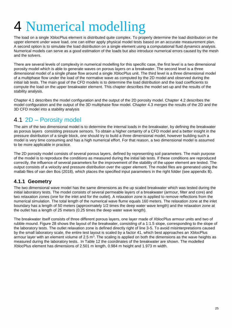
25

4 Numerical modelling The load on a single XblocPlus element is distributed quite complex. To properly determine the load distribution on the upper element under wave load, one can either apply physical model tests based on an accurate measurement plan. A second option is to simulate the load distribution on a single element using a computational fluid dynamics analysis. Numerical models can serve as a good estimation of the loads but also introduce numerical errors caused by the mesh and the solvers. There are several levels of complexity in numerical modelling for this specific case, the first level is a two dimensional porosity model which is able to generate waves on porous layers on a breakwater. The second level is a three dimensional model of a single phase flow around a single XblocPlus unit. The third level is a three dimensional model of a multiphase flow under the load of the normative wave as computed by the 2D model and observed during the initial lab tests. The main goal of the CFD models is to determine the load distribution and the load coefficients to compute the load on the upper breakwater element. This chapter describes the model set-up and the results of the stability analysis. Chapter 4.1 describes the model configuration and the output of the 2D porosity model. Chapter 4.2 describes the model configuration and the output of the 3D multiphase flow model. Chapter 4.3 merges the results of the 2D and the 3D CFD model into a stability analysis

4.1 2D – Porosity model The aim of the two dimensional model is to determine the internal loads in the breakwater, by defining the breakwater as porous layers consisting pressure sensors. To obtain a higher certainty of a CFD model and a better insight in the pressure distribution of a single block, one should try to build a three dimensional model, however building such a model is very time consuming and has a high numerical effort. For that reason, a two dimensional model is assumed to be more applicable in practice. The 2D porosity model consists of several porous layers, defined by representing soil parameters. The main purpose of the model is to reproduce the conditions as measured during the initial lab tests. If these conditions are reproduced correctly, the influence of several parameters for the improvement of the stability of the upper element are tested. The output consists of a velocity and pressure distribution over the upper element. The model files are generated using the matlab files of van den Bos (2018), which places the specified input parameters in the right folder (see appendix B).

4.1.1 Geometry

The two dimensional wave model has the same dimensions as the up scaled breakwater which was tested during the initial laboratory tests. The model consists of several permeable layers of a breakwater (armour, filter and core) and two relaxation zones (one for the inlet and for the outlet). A relaxation zone is applied to remove reflections from the numerical simulation. The total length of the numerical wave flume equals 160 meters. The relaxation zone at the inlet boundary has a length of 50 meters (approximately 1/2 times the deep water wave length) and the relaxation zone at the outlet has a length of 25 meters (0.25 times the deep water wave length). The breakwater itself consists of three different porous layers, one layer made of XblocPlus armour units and two of rubble mound. Figure 28 shows the layout of the breakwater, consisting of a 1:1.5 slope, corresponding to the slope of the laboratory tests. The outlet relaxation zone is defined directly right of line 3-5. To avoid misinterpretations caused by the small laboratory scale, the entire test layout is scaled by a factor 41, which best approaches an XblocPlus armour layer with an element volume of 2.5 m3. The scaling is applied on both the dimensions as the wave heights as measured during the laboratory tests. In Table 12 the coordinates of the breakwater are shown. The modelled XblocPlus element has dimensions of 2.501 m length, 0.984 m height and 1.973 m width.

26

Figure 28: Lay-out breakwater

Table 12: Coordinates breakwater

Location 0 1 2 3 4 5 6 7 8 9

X [m] 0 2.501 4.72 31.816 31.816 31.816 20.090 21.566 19.065 20.339

Y [m] 0 0 0 0 10.414 11.726 11.726 12.71 12.71 10.414

In Table 13, the input parameters for the individual layers is shown. The applied values for dn and N are based on the applied materials during the laboratory tests. The KC-number is determined using the formulation as mentioned in the literature review. The values for α and β are applied according to the initial research of van Gent (1995). It is known that these parameters are discussable, but serve as a good initial guess. Table 13: Soil parameters model

dn(50) [m] N KC α β

Armour 1.2 0.603 12.6 1000 1.1

Filter 0.656 0.4 23.1 1000 1.1

Core 0.282 0.4 53.7 1000 1.1

Wave generation

The incoming waves are generated according to a JONSWAP spectrum, with the scaled parameters from the initial laboratory tests. With a significant wave height of 3.5 meters, a peak period of 8.2 s and a gamma factor of 3.3. The mean wave period equals 7.04 seconds and the total run time equals 3400 s, which corresponds to a storm of 485 waves. More generated waves will increase the reliability of the model. As long as the generated wave spectrum consists of the same parameters as the target wave spectrum, one can assume that duration of the run is long enough.

Mesh

As a rule of thumb, one can say that at least 5-10 cells per wave height are required and 100-150 cells per wave length Paulsen (2017). To reduce the computational time as much as possible, the grid size should be defined as big as possible. As a compromise, the grid size is set to cells in both dx and dy direction of 0.4 m, which sets the number of cells per wave height to 8.75 and the number of cells per wave length to 262.2, for the deep water wave length. Since an aspect ratio of 1 is highly recommended around the still water level, the entire domain is separated in perfect squares.

Courant

The courant number determines how fast the flow travels through the computational domain. To increase the accuracy of a multiphase CFD model, the courant number should be as low as possible, to reduce an eventual numerical impulse from the water to the air of the domain as much as possible. A courant number of 0.3 is applied in the model Paulsen (2017).

4.1.2 Boundary conditions The boundary conditions for the model are separated in a part as described in the 0 folder and a part which describes the applied wave models in the system folder (2.8.1). Since the model consists of only two dimensions, the sides of the model are generated as empty patches. When applying an empty patch, the simulation is told not to solve the equations in that specific direction.

X

Y

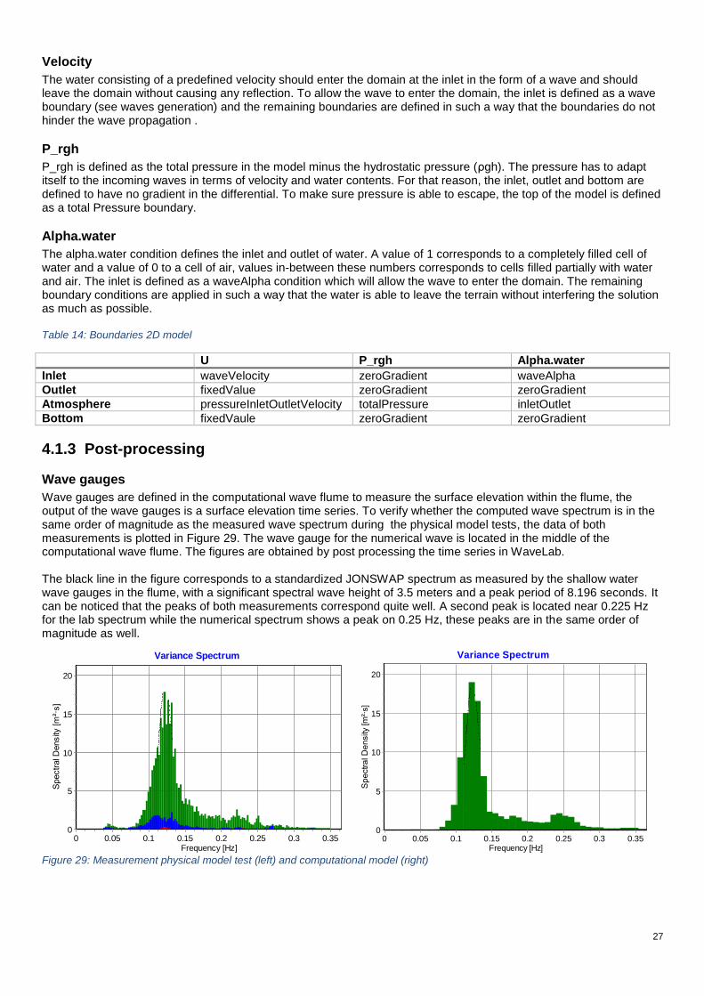
27

Velocity

The water consisting of a predefined velocity should enter the domain at the inlet in the form of a wave and should leave the domain without causing any reflection. To allow the wave to enter the domain, the inlet is defined as a wave boundary (see waves generation) and the remaining boundaries are defined in such a way that the boundaries do not hinder the wave propagation .

P_rgh

P_rgh is defined as the total pressure in the model minus the hydrostatic pressure (ρgh). The pressure has to adapt itself to the incoming waves in terms of velocity and water contents. For that reason, the inlet, outlet and bottom are defined to have no gradient in the differential. To make sure pressure is able to escape, the top of the model is defined as a total Pressure boundary.

Alpha.water

The alpha.water condition defines the inlet and outlet of water. A value of 1 corresponds to a completely filled cell of water and a value of 0 to a cell of air, values in-between these numbers corresponds to cells filled partially with water and air. The inlet is defined as a waveAlpha condition which will allow the wave to enter the domain. The remaining boundary conditions are applied in such a way that the water is able to leave the terrain without interfering the solution as much as possible. Table 14: Boundaries 2D model

U P_rgh Alpha.water

Inlet waveVelocity zeroGradient waveAlpha

Outlet fixedValue zeroGradient zeroGradient

Atmosphere pressureInletOutletVelocity totalPressure inletOutlet

Bottom fixedVaule zeroGradient zeroGradient

4.1.3 Post-processing

Wave gauges

Wave gauges are defined in the computational wave flume to measure the surface elevation within the flume, the output of the wave gauges is a surface elevation time series. To verify whether the computed wave spectrum is in the same order of magnitude as the measured wave spectrum during the physical model tests, the data of both measurements is plotted in Figure 29. The wave gauge for the numerical wave is located in the middle of the computational wave flume. The figures are obtained by post processing the time series in WaveLab. The black line in the figure corresponds to a standardized JONSWAP spectrum as measured by the shallow water wave gauges in the flume, with a significant spectral wave height of 3.5 meters and a peak period of 8.196 seconds. It can be noticed that the peaks of both measurements correspond quite well. A second peak is located near 0.225 Hz for the lab spectrum while the numerical spectrum shows a peak on 0.25 Hz, these peaks are in the same order of magnitude as well.

Figure 29: Measurement physical model test (left) and computational model (right)

Variance Spectrum

Incident Reflected Noise/Error

Frequency [Hz]0.350.30.250.20.150.10.050

Spectr

al D

ensity

[m

²·s]

20

15

10

5

0

Variance Spectrum

Frequency [Hz]0.350.30.250.20.150.10.050

Sp

ectr

al D

en

sity [m

²·s]

20

15

10

5

0

28

Pressure gauges

To measure the local parameters at the simplified upper element, pressure gauges are located around the entire element. During the computation, these gauges store the water content of the numerical cell (alpha.water), the velocity in all three dimensions (Uz equals zero), the static pressure p on the element and the p_rgh (pressure minus ρgh, where h is the distance from a certain reference level). The distribution of the pressure gauges is shown in Figure 30. The distance in-between two horizontal points equals 0.5002 meters and 0.4935 meters in vertical direction (under a 1:1.5 slope).

Figure 30: Pressure gauge around upper element without (left) and with (right) XblocPlus

The current pressure gauge distribution is representative for a layer without the contours of a XblocPlus element. However, when placing the contours of a real XblocPlus element on top of the simplified element, one can see that several pressure gauges do not represent a single unit quite well. Therefore wave gauge 0 and 1, which will increase the momentum around the rotation points significantly, should be ignored. One may propose to remove the triangle 0-1-13, however when adding the second highest element, one can see that this area is still required for the porous resistance of the armour layer (Figure 31).

Figure 31: Pressure gauges with second element

Data reduction

After each computational time step, a data point is added to the list. To reduce the length of the list, a criteria for the water content in the computation cells is added (alpha.water, which ranges from 1 to 0). If the cell contains less than 1% water, all of the computed data is removed and all the empty rows are removed (corresponding to no wave impact on the element). This reduces the total dataset by approximately 2/3th of the original length and reduces the computation time for the momentum analysis. Setting the water content limit also reduces the high velocity peaks caused by the numerical impulse in-between the water and the air.

Run-up velocity

The maximum measured velocity at pressure gauge 0 (location where the velocity is maximum according to the model configuration) is equal to 3.43 m/s, which corresponds quite well with the run-up velocity of approximately 3.2 m/s as measured in the wave flume. During the same wave a couple seconds later, the maximum run-up velocity at pressure gauge 13 and 12 are determined to be 2.43 and 2.04 m/s respectively. In Figure 32, the wave with the highest run-up velocity on the breakwater is shown.

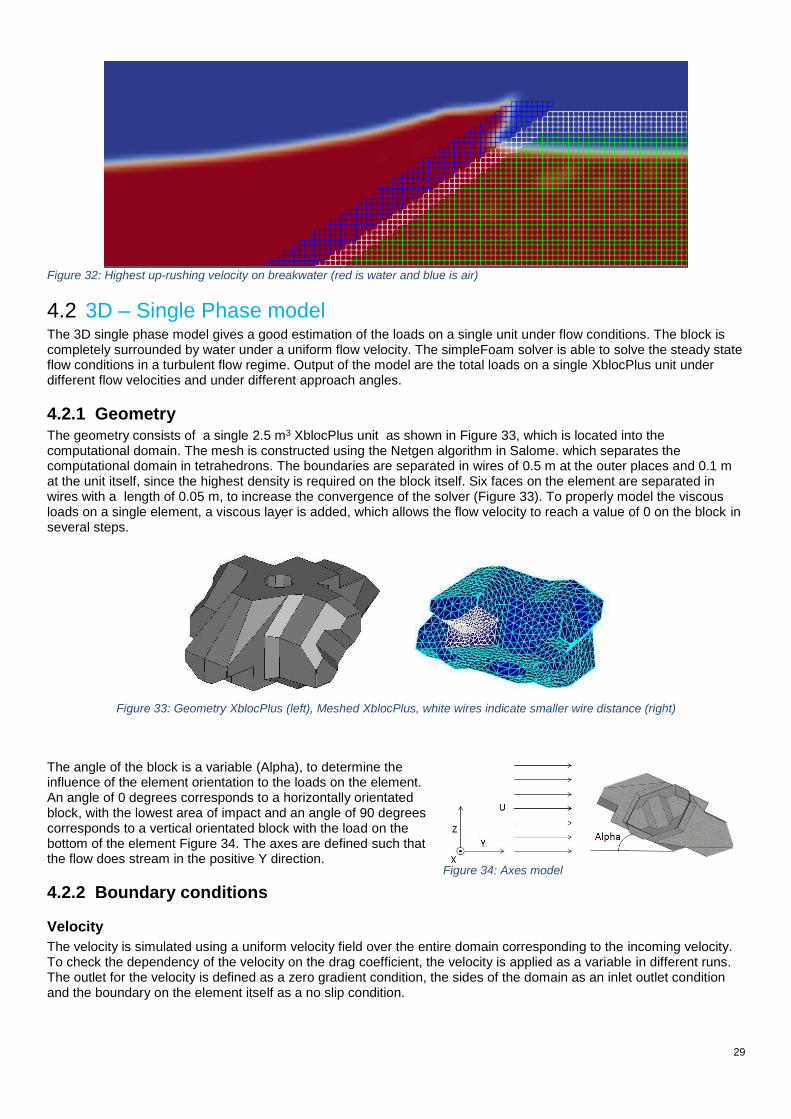
29

Figure 34: Axes model

Figure 32: Highest up-rushing velocity on breakwater (red is water and blue is air)

4.2 3D – Single Phase model The 3D single phase model gives a good estimation of the loads on a single unit under flow conditions. The block is completely surrounded by water under a uniform flow velocity. The simpleFoam solver is able to solve the steady state flow conditions in a turbulent flow regime. Output of the model are the total loads on a single XblocPlus unit under different flow velocities and under different approach angles.

4.2.1 Geometry

The geometry consists of a single 2.5 m3 XblocPlus unit as shown in Figure 33, which is located into the computational domain. The mesh is constructed using the Netgen algorithm in Salome. which separates the computational domain in tetrahedrons. The boundaries are separated in wires of 0.5 m at the outer places and 0.1 m at the unit itself, since the highest density is required on the block itself. Six faces on the element are separated in wires with a length of 0.05 m, to increase the convergence of the solver (Figure 33). To properly model the viscous loads on a single element, a viscous layer is added, which allows the flow velocity to reach a value of 0 on the block in several steps.

Figure 33: Geometry XblocPlus (left), Meshed XblocPlus, white wires indicate smaller wire distance (right)

The angle of the block is a variable (Alpha), to determine the influence of the element orientation to the loads on the element. An angle of 0 degrees corresponds to a horizontally orientated block, with the lowest area of impact and an angle of 90 degrees corresponds to a vertical orientated block with the load on the bottom of the element Figure 34. The axes are defined such that the flow does stream in the positive Y direction.

4.2.2 Boundary conditions

Velocity

The velocity is simulated using a uniform velocity field over the entire domain corresponding to the incoming velocity. To check the dependency of the velocity on the drag coefficient, the velocity is applied as a variable in different runs. The outlet for the velocity is defined as a zero gradient condition, the sides of the domain as an inlet outlet condition and the boundary on the element itself as a no slip condition.

30

Pressure

The initial pressure during the initial conditions is set to zero, to reduce the pressure gradients over the domain as much as possible, the only pressure gradients are expected around the element itself. The inlet and the element boundary is defined as a zero gradient, the outlet as a fixed value set to 0 and the sides are defined as an outlet inlet boundary .

K - Epsilon

The initial conditions for the turbulent kinetic energy are determined using estimated values. According to OpenFoam guide (2018), the turbulence kinetic energy can be estimated using:

𝑘 =3

2(𝐼|𝑢𝑟𝑒𝑓|)

2

Where I is the turbulent intensity which is in-between 5 and 20% for high turbulent flows and uref the incoming flow velocity. Epsilon can be estimated using:

𝜀 =𝐶𝜇

0.75𝑘1.5

𝐿

Cμ is an empirical parameter and equals 0.09 most of the times and L is the turbulent length scale, which is set to the width of the element. If the simulation appears to be unstable, the initial values can be increased to properly simulate the turbulent behaviour. The inlets are defined as a uniform fixed value, equal to the estimated turbulent values. The outlet and the sides of the domain are defined as a zero gradient condition and the boundary condition on the element itself as a wall function.

Nut

The turbulent viscosity is a parameter which forces the diffusivity of the turbulent eddies to either increase or decrease. All of the nut boundaries of the computational domain are defined as a calculated boundary, which automatically determines the right turbulent diffusivity. Table 15: Boundaries 3D- model

U P K-Epsilon Nut

Front fixedValue zeroGradient fixedValue calculated

Back zeroGradient fixedValue zeroGradient calculated

Side inletOutlet outletInlet zeroGradient Calculated

Block noSlip zeroGradient Kqr/epsilon WallFunction nutkWallFunction

4.2.3 Post-Processing OpenFoam is able to calculate the total load on an element using the force function. The function calculates the total force on an element by integrating both the normal pressure and the viscous stress over the surface area of a boundary cell. The total forces are defined as (OpenFoam, 2018):

𝑭𝒑 = ∑ 𝜌𝑖𝒔𝑓,𝑖 (𝑝𝑖 − 𝑝

𝑟𝑒𝑓)𝑖 𝑭𝝂 = ∑ 𝜌

𝑖𝒔𝑓,𝑖(𝜇𝑹𝑑𝑒𝑣)𝑖

Where S is the surface area of the element, p is the pressure, μ the viscosity and R the deviatoric Reynolds stress tensor (the Reynolds stress minus the hydrostatic stress). The output of the model is an integrated vector containing the forces in all the three dimensions. If the loads on the elements are known, the drag and the lift coefficient on the element can be determined. The flow area is defined as Dn

2, since this parameter is directly computable using the volume of a single element.

𝐶𝐷 =2𝐹𝐷

𝐷𝑛2𝜌𝑈2 𝐶𝐿 =

2𝐹𝐿

𝐷𝑛2𝜌𝑈2

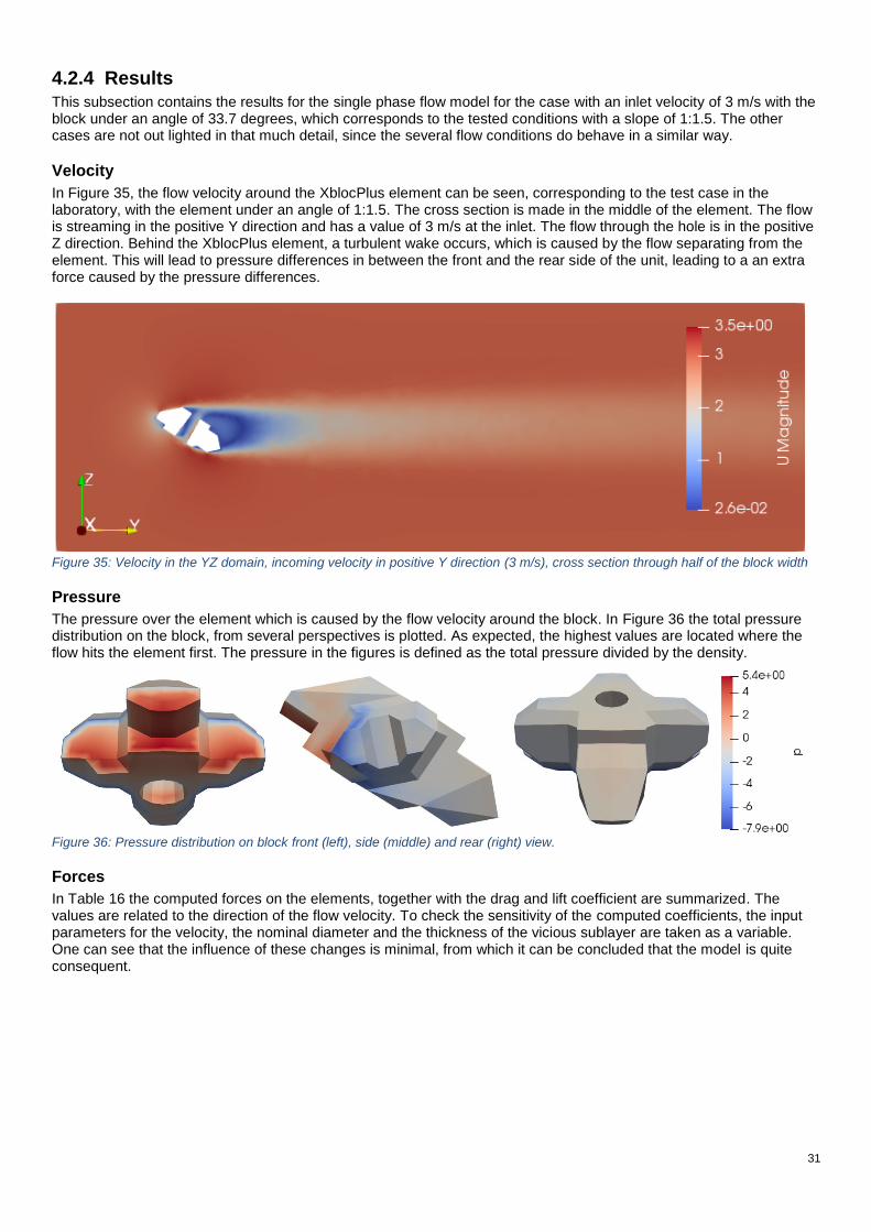
31

4.2.4 Results

This subsection contains the results for the single phase flow model for the case with an inlet velocity of 3 m/s with the block under an angle of 33.7 degrees, which corresponds to the tested conditions with a slope of 1:1.5. The other cases are not out lighted in that much detail, since the several flow conditions do behave in a similar way.

Velocity

In Figure 35, the flow velocity around the XblocPlus element can be seen, corresponding to the test case in the laboratory, with the element under an angle of 1:1.5. The cross section is made in the middle of the element. The flow is streaming in the positive Y direction and has a value of 3 m/s at the inlet. The flow through the hole is in the positive Z direction. Behind the XblocPlus element, a turbulent wake occurs, which is caused by the flow separating from the element. This will lead to pressure differences in between the front and the rear side of the unit, leading to a an extra force caused by the pressure differences.

Figure 35: Velocity in the YZ domain, incoming velocity in positive Y direction (3 m/s), cross section through half of the block width

Pressure

The pressure over the element which is caused by the flow velocity around the block. In Figure 36 the total pressure distribution on the block, from several perspectives is plotted. As expected, the highest values are located where the flow hits the element first. The pressure in the figures is defined as the total pressure divided by the density.

Figure 36: Pressure distribution on block front (left), side (middle) and rear (right) view.

Forces

In Table 16 the computed forces on the elements, together with the drag and lift coefficient are summarized. The values are related to the direction of the flow velocity. To check the sensitivity of the computed coefficients, the input parameters for the velocity, the nominal diameter and the thickness of the vicious sublayer are taken as a variable. One can see that the influence of these changes is minimal, from which it can be concluded that the model is quite consequent.

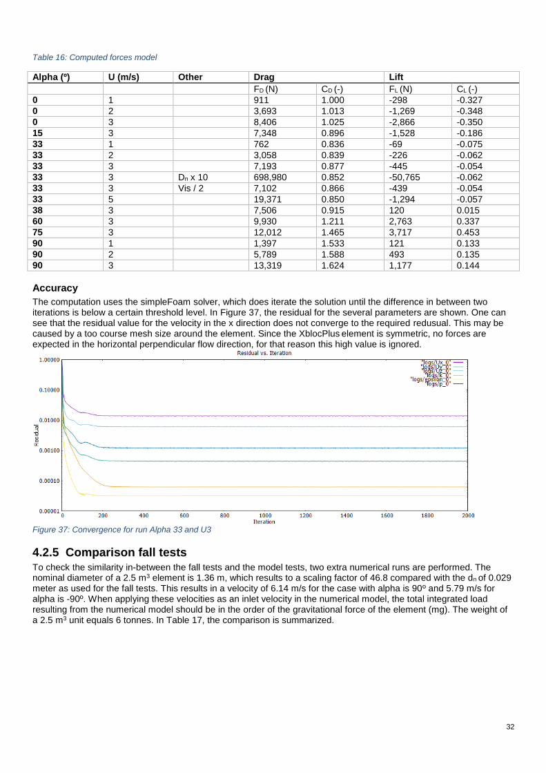
32

Table 16: Computed forces model

Alpha (º) U (m/s) Other Drag Lift

FD (N) CD (-) FL (N) CL (-)

0 1 911 1.000 -298 -0.327

0 2 3,693 1.013 -1,269 -0.348

0 3 8,406 1.025 -2,866 -0.350

15 3 7,348 0.896 -1,528 -0.186

33 1 762 0.836 -69 -0.075

33 2 3,058 0.839 -226 -0.062

33 3 7,193 0.877 -445 -0.054

33 3 Dn x 10 698,980 0.852 -50,765 -0.062

33 3 Vis / 2 7,102 0.866 -439 -0.054

33 5 19,371 0.850 -1,294 -0.057

38 3 7,506 0.915 120 0.015

60 3 9,930 1.211 2,763 0.337

75 3 12,012 1.465 3,717 0.453

90 1 1,397 1.533 121 0.133

90 2 5,789 1.588 493 0.135

90 3 13,319 1.624 1,177 0.144

Accuracy

The computation uses the simpleFoam solver, which does iterate the solution until the difference in between two iterations is below a certain threshold level. In Figure 37, the residual for the several parameters are shown. One can see that the residual value for the velocity in the x direction does not converge to the required redusual. This may be caused by a too course mesh size around the element. Since the XblocPlus element is symmetric, no forces are expected in the horizontal perpendicular flow direction, for that reason this high value is ignored.

Figure 37: Convergence for run Alpha 33 and U3

4.2.5 Comparison fall tests

To check the similarity in-between the fall tests and the model tests, two extra numerical runs are performed. The nominal diameter of a 2.5 m3 element is 1.36 m, which results to a scaling factor of 46.8 compared with the dn of 0.029 meter as used for the fall tests. This results in a velocity of 6.14 m/s for the case with alpha is 90º and 5.79 m/s for alpha is -90º. When applying these velocities as an inlet velocity in the numerical model, the total integrated load resulting from the numerical model should be in the order of the gravitational force of the element (mg). The weight of a 2.5 m3 unit equals 6 tonnes. In Table 17, the comparison is summarized.

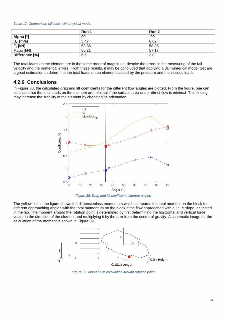
33

Table 17: Comparison fall tests with physical model

Run 1 Run 2

Alpha [º] 90 -90

Uin [m/s] 5.47 6.02

Fg [kN] 58.86 58.86

Fmodel [kN] 55.21 57.17

Difference [%] 6.6 3.0

The total loads on the element are in the same order of magnitude, despite the errors in the measuring of the fall velocity and the numerical errors. From these results, it may be concluded that applying a 3D numerical model test are a good estimation to determine the total loads on an element caused by the pressure and the viscous loads.

4.2.6 Conclusions

In Figure 38, the calculated drag and lift coefficients for the different flow angles are plotted. From the figure, one can conclude that the total loads on the element are minimal if the surface area under direct flow is minimal. This finding may increase the stability of the element by changing its orientation.

Figure 38: Drag and lift coefficient different angles

The yellow line in the figure shows the dimensionless momentum which compares the total moment on the block for different approaching angles with the total momentum on the block if the flow approached with a 1:1.5 slope, as tested in the lab. The moment around the rotation point is determined by first determining the horizontal and vertical force vector in the direction of the element and multiplying it by the arm from the centre of gravity. A schematic image for the calculation of the moment is shown in Figure 39.

Figure 39: Momentum calculation around rotation point

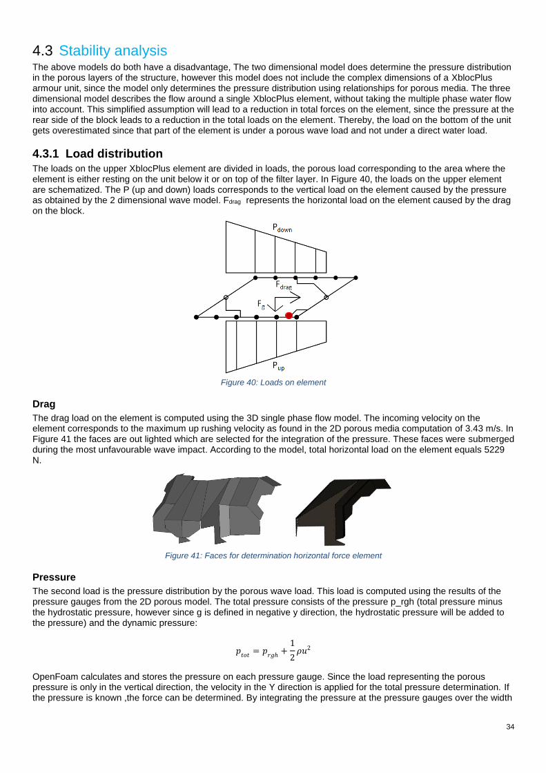
34

4.3 Stability analysis The above models do both have a disadvantage, The two dimensional model does determine the pressure distribution in the porous layers of the structure, however this model does not include the complex dimensions of a XblocPlus armour unit, since the model only determines the pressure distribution using relationships for porous media. The three dimensional model describes the flow around a single XblocPlus element, without taking the multiple phase water flow into account. This simplified assumption will lead to a reduction in total forces on the element, since the pressure at the rear side of the block leads to a reduction in the total loads on the element. Thereby, the load on the bottom of the unit gets overestimated since that part of the element is under a porous wave load and not under a direct water load.

4.3.1 Load distribution

The loads on the upper XblocPlus element are divided in loads, the porous load corresponding to the area where the element is either resting on the unit below it or on top of the filter layer. In Figure 40, the loads on the upper element are schematized. The P (up and down) loads corresponds to the vertical load on the element caused by the pressure as obtained by the 2 dimensional wave model. Fdrag represents the horizontal load on the element caused by the drag on the block.

Figure 40: Loads on element

Drag

The drag load on the element is computed using the 3D single phase flow model. The incoming velocity on the element corresponds to the maximum up rushing velocity as found in the 2D porous media computation of 3.43 m/s. In Figure 41 the faces are out lighted which are selected for the integration of the pressure. These faces were submerged during the most unfavourable wave impact. According to the model, total horizontal load on the element equals 5229 N.

Figure 41: Faces for determination horizontal force element

Pressure

The second load is the pressure distribution by the porous wave load. This load is computed using the results of the pressure gauges from the 2D porous model. The total pressure consists of the pressure p_rgh (total pressure minus the hydrostatic pressure, however since g is defined in negative y direction, the hydrostatic pressure will be added to the pressure) and the dynamic pressure:

𝑝𝑡𝑜𝑡

= 𝑝𝑟𝑔ℎ

+1

2𝜌𝑢2

OpenFoam calculates and stores the pressure on each pressure gauge. Since the load representing the porous pressure is only in the vertical direction, the velocity in the Y direction is applied for the total pressure determination. If the pressure is known ,the force can be determined. By integrating the pressure at the pressure gauges over the width

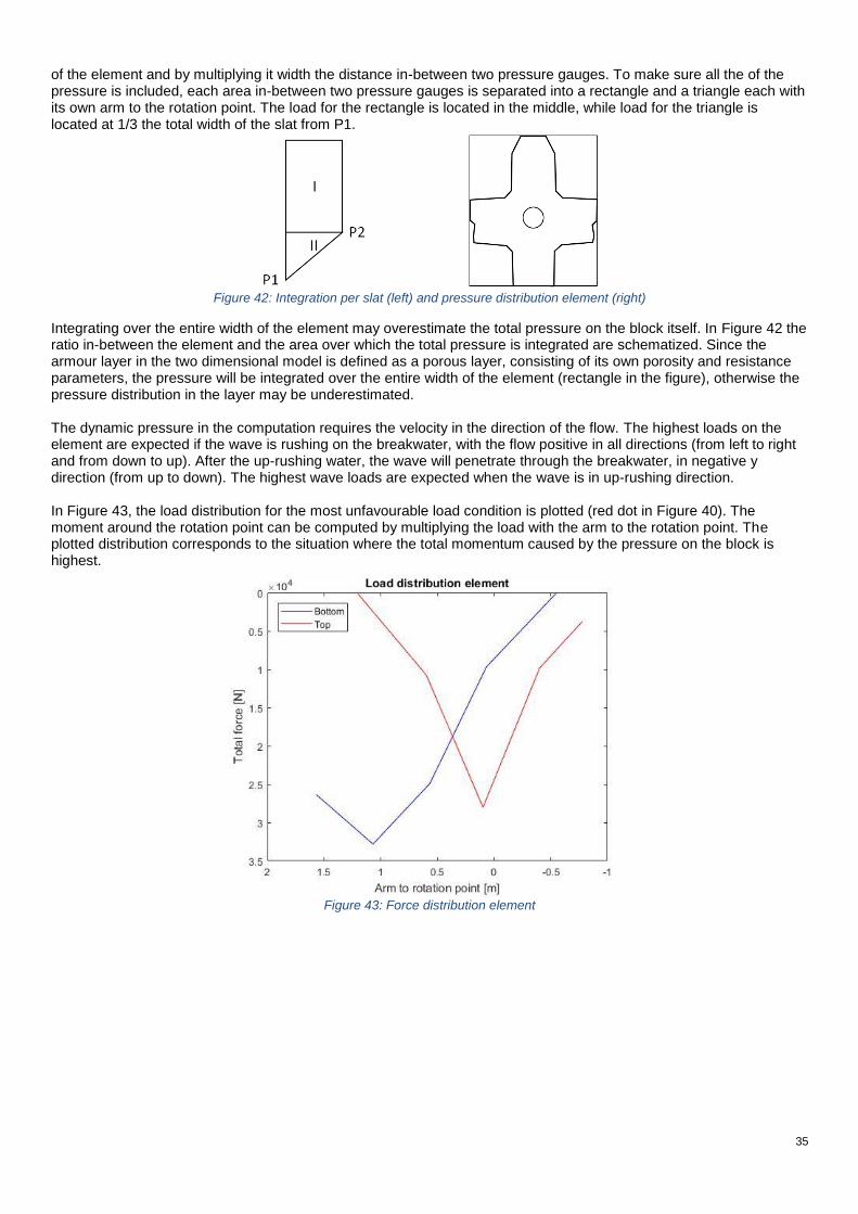
35

of the element and by multiplying it width the distance in-between two pressure gauges. To make sure all the of the pressure is included, each area in-between two pressure gauges is separated into a rectangle and a triangle each with its own arm to the rotation point. The load for the rectangle is located in the middle, while load for the triangle is located at 1/3 the total width of the slat from P1.

Figure 42: Integration per slat (left) and pressure distribution element (right)

Integrating over the entire width of the element may overestimate the total pressure on the block itself. In Figure 42 the ratio in-between the element and the area over which the total pressure is integrated are schematized. Since the armour layer in the two dimensional model is defined as a porous layer, consisting of its own porosity and resistance parameters, the pressure will be integrated over the entire width of the element (rectangle in the figure), otherwise the pressure distribution in the layer may be underestimated. The dynamic pressure in the computation requires the velocity in the direction of the flow. The highest loads on the element are expected if the wave is rushing on the breakwater, with the flow positive in all directions (from left to right and from down to up). After the up-rushing water, the wave will penetrate through the breakwater, in negative y direction (from up to down). The highest wave loads are expected when the wave is in up-rushing direction. In Figure 43, the load distribution for the most unfavourable load condition is plotted (red dot in Figure 40). The moment around the rotation point can be computed by multiplying the load with the arm to the rotation point. The plotted distribution corresponds to the situation where the total momentum caused by the pressure on the block is highest.

Figure 43: Force distribution element

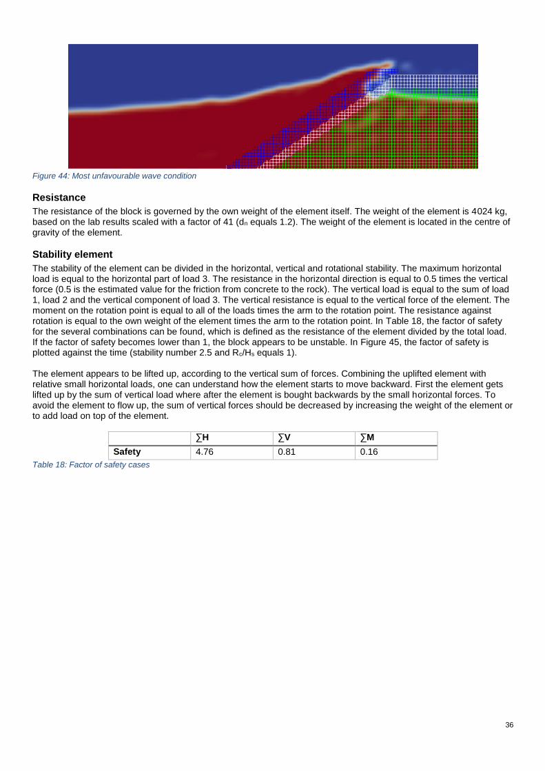
36

Figure 44: Most unfavourable wave condition

Resistance

The resistance of the block is governed by the own weight of the element itself. The weight of the element is 4024 kg, based on the lab results scaled with a factor of 41 (dn equals 1.2). The weight of the element is located in the centre of gravity of the element.

Stability element

The stability of the element can be divided in the horizontal, vertical and rotational stability. The maximum horizontal load is equal to the horizontal part of load 3. The resistance in the horizontal direction is equal to 0.5 times the vertical force (0.5 is the estimated value for the friction from concrete to the rock). The vertical load is equal to the sum of load 1, load 2 and the vertical component of load 3. The vertical resistance is equal to the vertical force of the element. The moment on the rotation point is equal to all of the loads times the arm to the rotation point. The resistance against rotation is equal to the own weight of the element times the arm to the rotation point. In Table 18, the factor of safety for the several combinations can be found, which is defined as the resistance of the element divided by the total load. If the factor of safety becomes lower than 1, the block appears to be unstable. In Figure 45, the factor of safety is plotted against the time (stability number 2.5 and Rc/Hs equals 1). The element appears to be lifted up, according to the vertical sum of forces. Combining the uplifted element with relative small horizontal loads, one can understand how the element starts to move backward. First the element gets lifted up by the sum of vertical load where after the element is bought backwards by the small horizontal forces. To avoid the element to flow up, the sum of vertical forces should be decreased by increasing the weight of the element or to add load on top of the element.

∑H ∑V ∑M

Safety 4.76 0.81 0.16

Table 18: Factor of safety cases

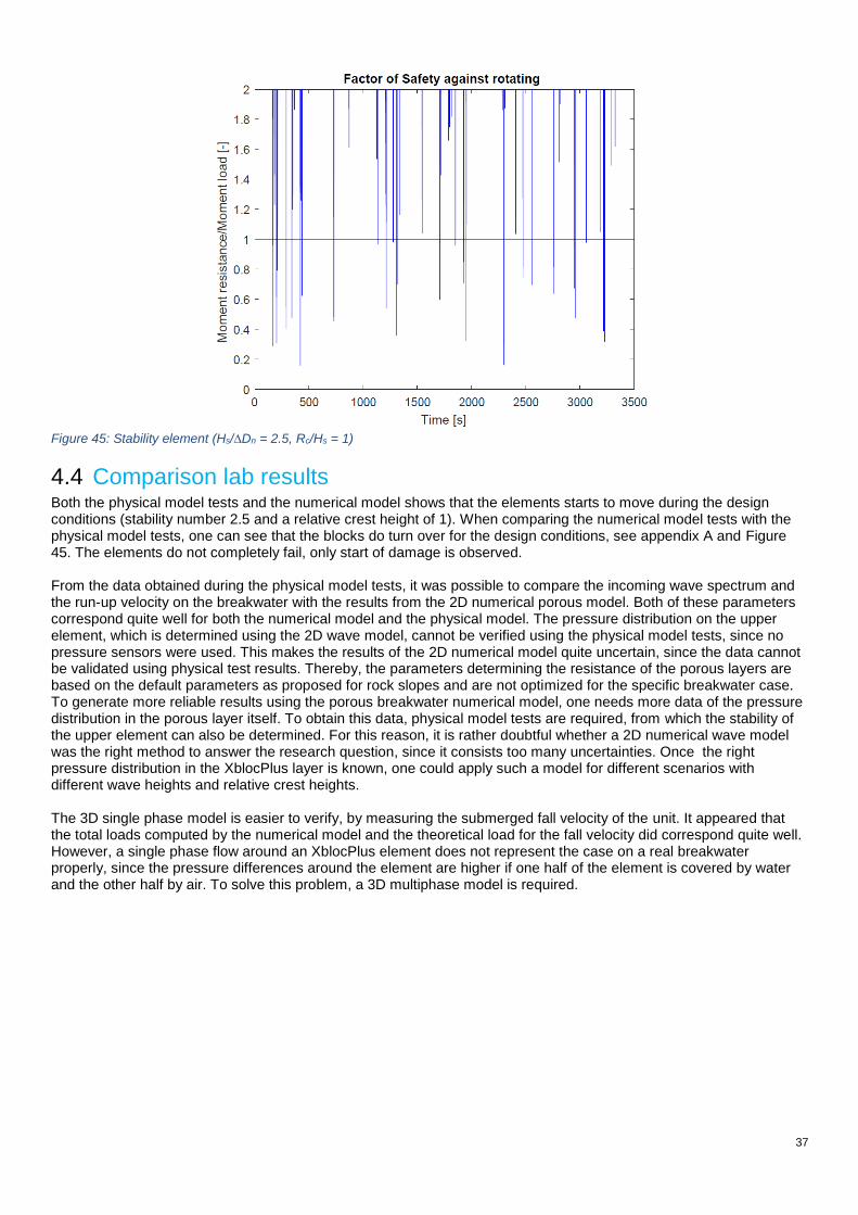
37

Figure 45: Stability element (Hs/∆Dn = 2.5, Rc/Hs = 1)

4.4 Comparison lab results Both the physical model tests and the numerical model shows that the elements starts to move during the design conditions (stability number 2.5 and a relative crest height of 1). When comparing the numerical model tests with the physical model tests, one can see that the blocks do turn over for the design conditions, see appendix A and Figure 45. The elements do not completely fail, only start of damage is observed. From the data obtained during the physical model tests, it was possible to compare the incoming wave spectrum and the run-up velocity on the breakwater with the results from the 2D numerical porous model. Both of these parameters correspond quite well for both the numerical model and the physical model. The pressure distribution on the upper element, which is determined using the 2D wave model, cannot be verified using the physical model tests, since no pressure sensors were used. This makes the results of the 2D numerical model quite uncertain, since the data cannot be validated using physical test results. Thereby, the parameters determining the resistance of the porous layers are based on the default parameters as proposed for rock slopes and are not optimized for the specific breakwater case. To generate more reliable results using the porous breakwater numerical model, one needs more data of the pressure distribution in the porous layer itself. To obtain this data, physical model tests are required, from which the stability of the upper element can also be determined. For this reason, it is rather doubtful whether a 2D numerical wave model was the right method to answer the research question, since it consists too many uncertainties. Once the right pressure distribution in the XblocPlus layer is known, one could apply such a model for different scenarios with different wave heights and relative crest heights. The 3D single phase model is easier to verify, by measuring the submerged fall velocity of the unit. It appeared that the total loads computed by the numerical model and the theoretical load for the fall velocity did correspond quite well. However, a single phase flow around an XblocPlus element does not represent the case on a real breakwater properly, since the pressure differences around the element are higher if one half of the element is covered by water and the other half by air. To solve this problem, a 3D multiphase model is required.

38

5 Discussion This chapter describes the possibilities to increase the accuracy of the applied models and proposes how the stability of the upper element can be stabilized. Based on the conclusions of the physical model tests and the uncertainties caused within the numerical models, optimizations are proposed to optimize the stability of XblocPlus crest element.

5.1 Physical model tests The time to apply physical model tests during the process was limited. Thereby, it was not possible to create a structure where all of the dimensions could be determined individually, since the model had to be reused for other purposes. The aim of the tests was to find the parameters important of the stability of the upper element, which are found. However, with the new insights from those conclusions and the rest of the process, some optimisations are proposed.

5.1.1 Foreshore

During the physical model tests, a foreshore was located in front of the breakwater. For that reason, heavy wave breaking was observed during the physical model tests, leading to energy reduction when the wave hits the breakwater. This wave breaking leads to a difference in wave height in the deep water (at the wave paddle) and the shallow water (toe of the structure). The target wave height and stability numbers are based on the target deep water wave height. During further tests, it may be more suitable to test the structure in deep water wave conditions, to make sure the reduction in wave energy in-between the wave paddle and the structure is limited (see chapter Steep foreshore2.4.5). Secondly, the shallow water wave gauges were not located in an optimal position. Since heavy wave breaking occurred on the foreshore, the wave gauges should be located closer to the toe of the breakwater. This should be done to reduce the difference in measured wave energy at the wave gauge and the real wave energy at the toe of the structure as much as possible.

5.1.2 Placement units

The placement of the top unit is important for the stability of the upper element of a XblocPlus armour layer. The smaller the distance from the tail of the element to the filter layer, the higher the resistance against rotation of the unit. During the physical model tests, this distance is not measured. For that reason, accurate conclusions relating the change of failure with the distance in-between the tail and the filter layer, cannot be drawn. It was found that increasing the support under the upper element leads to an increment in stability. For further researches, one should measure this distance for each individual element and compare it with the time of failure of the element. From this, it is possible to define requirements on the quality of the transition from slope to crest of the filter layer.

5.1.3 Slope

The XblocPlus units are designed for 3:4 slopes, however this thesis focusses on a 2:3 slope, since the available breakwater during the physical model tests was constructed with that slope. The slope applied in the thesis is less steep than the slope of a real XblocPlus breakwater. The stepper a slope, the more overtopping is expected, the higher the total loads on the crest will be (equation as stated in 2.5.2). The effects for the stability of the upper element are expected to behave the same in both of the cases, probably with higher loads on the individual elements.

5.1.4 Run-up velocities

During the physical model tests, the run-up velocities were visually observed, which gives a good indication of the order of magnitude of the expected up-rushing velocities. The run-up velocities are measured with an accuracy of 0.5 cm/frame, which corresponds to 0.125 m/s in model scale, which is quite large for a 0.5 m/s maximum up-rushing velocity.

5.1.5 Fall tests The applied fall tests showed heavy whirling of the element when falling down. To avoid this whirling, one should find some way to hold the element completely horizontal, for example by attaching the element to stiff and vertical wire. This will influence the turbulent behaviour around the element but it is required to drop the element from higher distances. The applied fall tests in the bucket are assumed to be of an acceptable accuracy, despite the small vertical distance.

39

5.2 Numerical model The numerical models as described in this report are validated using the visually observed run-up velocity on the slope, the comparison of the incoming wave spectrum and the applied fall tests. These parameters can estimate the total loads on the crest element quite well, however for more certainty regarding the stability analysis performed with these models, more validation of the models is required. This chapter describes how to improve the accuracy of the numerical models which are used during this study.

5.2.1 Soil parameters To improve the performance of the 2 dimensional porous wave model, more information about the water pressure distribution is required in the porous layer of a breakwater, achieved by physical model tests. In the current research, the soil parameters of the model are chosen as commonly used values as described in several researches. These values are often verified for breakwaters consisting of rock. When applying other materials, these parameters should be redefined. To optimize the soil parameters, which serve as an input of the model, one should measure the total pressure during physical model tests and try to obtain the same values in the numerical model, by changing the soil parameters as the porosity and the resistance parameters as stated in chapter 2.8.2. The best method to calibrate the parameters is to perform physical model tests using a regular wave, measure the pressures at the points of interest and thereafter run the numerical model with the same regular wave parameters. Using a regular wave spectrum reduces the run time of the numerical model, since only a few waves needs to be modelled. If the soil parameters are determined properly, one could insert the values for irregular waves with different breakwater dimensions. As a trail, the α value is set to 500 and the β value to 2 which is proposed by Jensen (2014), who calibrated the porous parameters using the flow through a porous dam. The results of the run is a factor of safety of 0.23 for the sum of moments and a factor of safety of 0.95 for the sum of vertical forces, comparable to the results of a run with the default parameters of 1000 and 1. The run up velocities calculated are equal to 3.2, 2.3 and 1.7 m/s from the lower left probe to the upper left probe of the element. The gradient in the run-up velocity is higher than the run-up velocity observed during the model tests. For that reason it is assumed that the default parameters are more suitable for this problem than the values proposed by Jensen, for this specific case.

5.2.2 3D multi-phase modelling The best method to compute the load distribution on the crest element is by modelling the upper elements in a 3 dimensional multi-phase model. An attempt to run such a 3 dimensional multi-phase model is done, but it was not possible to make the model stable. In appendix C, the input of this model is described. Building such a model will result in a reliable output if the incoming wave is modelled properly, however building such a model is very time consuming and has a high numerical effort. For that reason it is doubtable whether such a model is a good solution for design purposes.

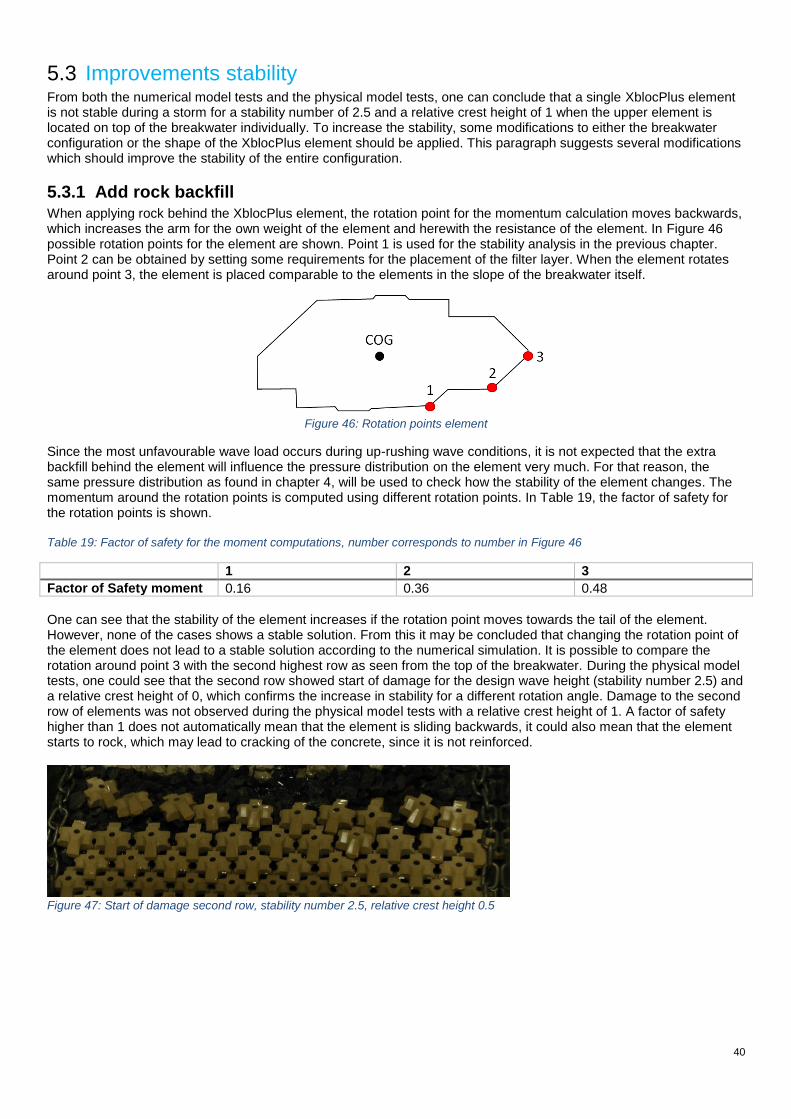
40

5.3 Improvements stability From both the numerical model tests and the physical model tests, one can conclude that a single XblocPlus element is not stable during a storm for a stability number of 2.5 and a relative crest height of 1 when the upper element is located on top of the breakwater individually. To increase the stability, some modifications to either the breakwater configuration or the shape of the XblocPlus element should be applied. This paragraph suggests several modifications which should improve the stability of the entire configuration.

5.3.1 Add rock backfill When applying rock behind the XblocPlus element, the rotation point for the momentum calculation moves backwards, which increases the arm for the own weight of the element and herewith the resistance of the element. In Figure 46 possible rotation points for the element are shown. Point 1 is used for the stability analysis in the previous chapter. Point 2 can be obtained by setting some requirements for the placement of the filter layer. When the element rotates around point 3, the element is placed comparable to the elements in the slope of the breakwater itself.

Figure 46: Rotation points element

Since the most unfavourable wave load occurs during up-rushing wave conditions, it is not expected that the extra backfill behind the element will influence the pressure distribution on the element very much. For that reason, the same pressure distribution as found in chapter 4, will be used to check how the stability of the element changes. The momentum around the rotation points is computed using different rotation points. In Table 19, the factor of safety for the rotation points is shown. Table 19: Factor of safety for the moment computations, number corresponds to number in Figure 46

1 2 3

Factor of Safety moment 0.16 0.36 0.48

One can see that the stability of the element increases if the rotation point moves towards the tail of the element. However, none of the cases shows a stable solution. From this it may be concluded that changing the rotation point of the element does not lead to a stable solution according to the numerical simulation. It is possible to compare the rotation around point 3 with the second highest row as seen from the top of the breakwater. During the physical model tests, one could see that the second row showed start of damage for the design wave height (stability number 2.5) and a relative crest height of 0, which confirms the increase in stability for a different rotation angle. Damage to the second row of elements was not observed during the physical model tests with a relative crest height of 1. A factor of safety higher than 1 does not automatically mean that the element is sliding backwards, it could also mean that the element starts to rock, which may lead to cracking of the concrete, since it is not reinforced.

Figure 47: Start of damage second row, stability number 2.5, relative crest height 0.5

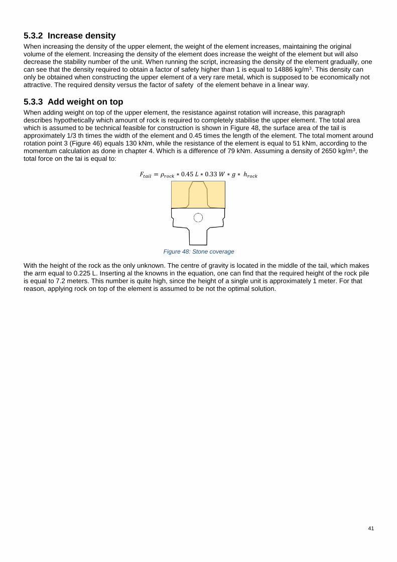
41

5.3.2 Increase density

When increasing the density of the upper element, the weight of the element increases, maintaining the original volume of the element. Increasing the density of the element does increase the weight of the element but will also decrease the stability number of the unit. When running the script, increasing the density of the element gradually, one can see that the density required to obtain a factor of safety higher than 1 is equal to 14886 kg/m3. This density can only be obtained when constructing the upper element of a very rare metal, which is supposed to be economically not attractive. The required density versus the factor of safety of the element behave in a linear way.

5.3.3 Add weight on top When adding weight on top of the upper element, the resistance against rotation will increase, this paragraph describes hypothetically which amount of rock is required to completely stabilise the upper element. The total area which is assumed to be technical feasible for construction is shown in Figure 48, the surface area of the tail is approximately 1/3 th times the width of the element and 0.45 times the length of the element. The total moment around rotation point 3 (Figure 46) equals 130 kNm, while the resistance of the element is equal to 51 kNm, according to the momentum calculation as done in chapter 4. Which is a difference of 79 kNm. Assuming a density of 2650 kg/m3, the total force on the tai is equal to:

𝐹𝑡𝑎𝑖𝑙 = 𝜌𝑟𝑜𝑐𝑘 ∗ 0.45𝐿 ∗ 0.33𝑊 ∗ 𝑔 ∗ℎ𝑟𝑜𝑐𝑘

Figure 48: Stone coverage

With the height of the rock as the only unknown. The centre of gravity is located in the middle of the tail, which makes the arm equal to 0.225 L. Inserting al the knowns in the equation, one can find that the required height of the rock pile is equal to 7.2 meters. This number is quite high, since the height of a single unit is approximately 1 meter. For that reason, applying rock on top of the element is assumed to be not the optimal solution.

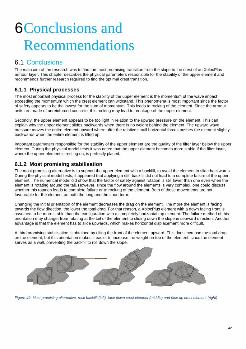
42

6 Conclusions and

Recommendations 6.1 Conclusions The main aim of the research was to find the most promising transition from the slope to the crest of an XblocPlus armour layer. This chapter describes the physical parameters responsible for the stability of the upper element and recommends further research required to find the optimal crest transition.

6.1.1 Physical processes

The most important physical process for the stability of the upper element is the momentum of the wave impact exceeding the momentum which the crest element can withstand. This phenomena is most important since the factor of safety appears to be the lowest for the sum of momentum. This leads to rocking of the element. Since the armour units are made of unreinforced concrete, this rocking may lead to breakage of the upper element. Secondly, the upper element appears to be too light in relation to the upward pressure on the element. This can explain why the upper element slides backwards when there is no weight behind the element. The upward wave pressure moves the entire element upward where after the relative small horizontal forces pushes the element slightly backwards when the entire element is lifted up. Important parameters responsible for the stability of the upper element are the quality of the filter layer below the upper element. During the physical model tests it was noted that the upper element becomes more stable if the filter layer, where the upper element is resting on, is perfectly placed.

6.1.2 Most promising stabilisation The most promising alternative is to support the upper element with a backfill, to avoid the element to slide backwards. During the physical model tests, it appeared that applying a stiff backfill did not lead to a complete failure of the upper element. The numerical model did show that the factor of safety against rotation is still lower than one even when the element is rotating around the tail. However, since the flow around the elements is very complex, one could discuss whether this rotation leads to complete failure or to rocking of the element. Both of these movements are not favourable for the element on both the long and the short term. Changing the initial orientation of the element decreases the drag on the element. The more the element is facing towards the flow direction, the lower the total drag. For that reason, a XblocPlus element with a down facing front is assumed to be more stable than the configuration with a completely horizontal top element. The failure method of this orientation may change, from rotating at the tail of the element to sliding down the slope in seaward direction. Another advantage is that the element has to slide upwards, which makes horizontal displacement more difficult. A third promising stabilisation is obtained by tilting the front of the element upward. This does increase the total drag on the element, but this orientation makes it easier to increase the weight on top of the element, since the element serves as a wall, preventing the backfill to roll down the slope.

Figure 49: Most promising alternative, rock backfill (left), face down crest element (middle) and face up crest element (right)

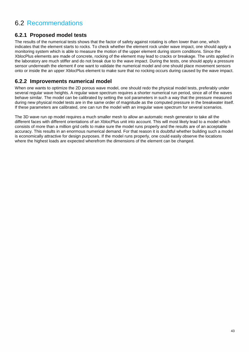
43

6.2 Recommendations

6.2.1 Proposed model tests The results of the numerical tests shows that the factor of safety against rotating is often lower than one, which indicates that the element starts to rocks. To check whether the element rock under wave impact, one should apply a monitoring system which is able to measure the motion of the upper element during storm conditions. Since the XblocPlus elements are made of concrete, rocking of the element may lead to cracks or breakage. The units applied in the laboratory are much stiffer and do not break due to the wave impact. During the tests, one should apply a pressure sensor underneath the element if one want to validate the numerical model and one should place movement sensors onto or inside the an upper XblocPlus element to make sure that no rocking occurs during caused by the wave impact.

6.2.2 Improvements numerical model When one wants to optimize the 2D porous wave model, one should redo the physical model tests, preferably under several regular wave heights. A regular wave spectrum requires a shorter numerical run period, since all of the waves behave similar. The model can be calibrated by setting the soil parameters in such a way that the pressure measured during new physical model tests are in the same order of magnitude as the computed pressure in the breakwater itself. If these parameters are calibrated, one can run the model with an irregular wave spectrum for several scenarios. The 3D wave run op model requires a much smaller mesh to allow an automatic mesh generator to take all the different faces with different orientations of an XblocPlus unit into account. This will most likely lead to a model which consists of more than a million grid cells to make sure the model runs properly and the results are of an acceptable accuracy. This results in an enormous numerical demand. For that reason it is doubtful whether building such a model is economically attractive for design purposes. If the model runs properly, one could easily observe the locations where the highest loads are expected wherefrom the dimensions of the element can be changed.

44

Bibliography Allsop, N. J. (1996). Guidelines for single layer hollow cube armour systems for breakwaters and related marine structures. Wellingfort: HR Wellingford Battjes, J.A. (1974) Computation of Set-up, longshore currents, run-up and overtopping due to wind-generated waves, University of Technology, Delft, The Netherlands Besley, P. (1999). Overtopping of seawalls – design and assessment manual. R & D Technical Report W 178, Environment Agency, Bristol, ISBN 1 85705 069 X. Van den Bos (2018), matlab2foam files, draft version. BusinessDictionary.com. Retrieved January 21, 2018, from BusinessDictionary.com website: http://www.businessdictionary.com/definition/constructability.html Bruce, T. van der Meer, J. W., Franco, L., Pearson, J.M. (2007), A comparison of overtopping performance of different rubble mount breakwater units, ICCE-2006, abstract number 1705. CIRIA, CUR, CETMEF (2007), The rock manual. The use of rock in hydraulic engineering (2nd edition). C683, CIRIA, London Dai, Y.B., Kamel, A.M. (1969), Scale tests for rubble-mound breakwaters, U.S. Army Engineer Waterways Experiment Station, Corps of Engineers, Vicksburg, Mississippi. De Rover, R. (2007) Breakwater stability with damaged single layer armour units, M.Sc.-thesis, Delft University of Technology, Delft, The Netherlands Delta Marine Consutlants (2014), Guidelines for Xbloc Concept Designs, Delta Marine Consultants, Gouda Moreno A.J. (2017), Experimental study on the wave overtopping performance of Xbloc+ armour unit Paulsen, B.T., Jacobsen, N.G. (2017), Slides waves2Foam, Delft software days 2017, Delft, the Netherlands, Deltares EurOtop, (2016). Manual on wave overtopping of sea defences and related structures. An overtopping manual largely based on European research, but for worldwide application. Van der Meer, J.W., Allsop, N.W.H., Bruce, T., De Rouck, J., Kortenhaus, A., Pullen, T., Schüttrumpf, H., Troch, P. and Zanuttigh, B., www.overtopping-manual.com. Hasselmann, K., Barnett, T. P., Bouws, E., Carlson, H., Cartwright, Enke, D. E. K., Ewing, J. A. Gienapp, H., Hasselmann, D. E., Kruseman, P., Meerburg, A., Muller, P., Olbers, D.J., Richter, D. J., K., Sell, W, Walden, H. (1973) Meaurements of Wind-Wave Growth and Swell Decay during the Joint North Sea Wave Project (JONSWAP), Herausgegeben vom Deutschen Hydrographischen Institut Hald, T. (1998). Wave Induced Loading and Stability of Rubble Mound Breakwaters. Aalborg: Hydraulics & Coastal Engineering Laboratory, Department of Civil Engineering, Aalborg University. Series Paper, No. 18 Hoerner, S.F. (1965) Fluid-Dynamic drag. Practical information on aerodynamic drag and hydrodynamic resistance. Holthuijsen, L.H. (2007) Waves in Oceanic annd Coastal Waters. Cambridge university press, Cambridge. ISBN 978-0-521-12995-4 Hughes (1993) Physical models and laboratory techniques in coastal engineering. World scientific publisching co. pte. Ltd., Advanced series on ocean engineering – Volume 7, ISBN 981-02-1540-1 Jacobsen, N. G., Fuhrman, D. R., Fredsøe, J. (2012). A Wave Generation Toolbox for the Open-Source CFD Library: OpenFoam. International Journal for Numerical Methods in Fluids 70 (9), 1073-1088. Jacobsen, N.G. (2017) waves2Foam manual version 0.9 (SVN-revision 2113), Deltares Jacobsen, N.G., van Gent, R.A., Wolters, G. (2015) Numerical analysis of the interaction of irregular waves with two dimensional permeable coastal structures, Coastal engineering volume 102, August 2015.

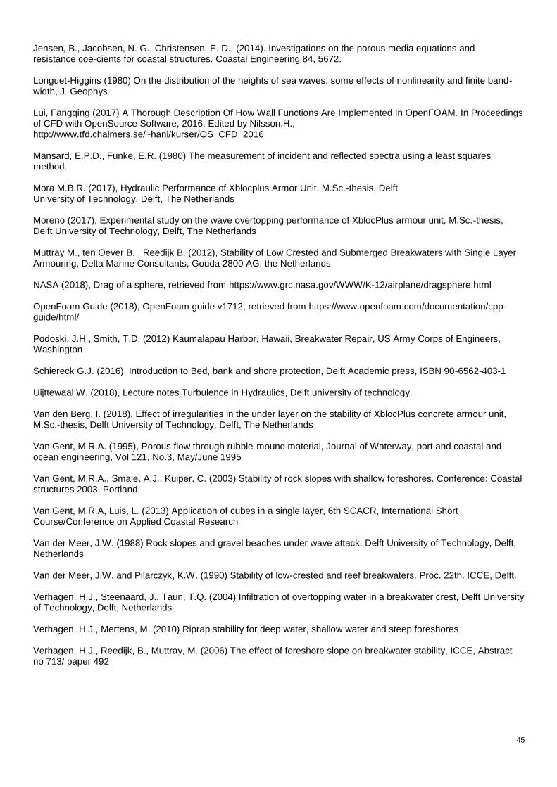
45

Jensen, B., Jacobsen, N. G., Christensen, E. D., (2014). Investigations on the porous media equations and resistance coe-cients for coastal structures. Coastal Engineering 84, 5672. Longuet-Higgins (1980) On the distribution of the heights of sea waves: some effects of nonlinearity and finite band-width, J. Geophys Lui, Fangqing (2017) A Thorough Description Of How Wall Functions Are Implemented In OpenFOAM. In Proceedings of CFD with OpenSource Software, 2016, Edited by Nilsson.H., http://www.tfd.chalmers.se/~hani/kurser/OS_CFD_2016 Mansard, E.P.D., Funke, E.R. (1980) The measurement of incident and reflected spectra using a least squares method. Mora M.B.R. (2017), Hydraulic Performance of Xblocplus Armor Unit. M.Sc.-thesis, Delft University of Technology, Delft, The Netherlands Moreno (2017), Experimental study on the wave overtopping performance of XblocPlus armour unit, M.Sc.-thesis, Delft University of Technology, Delft, The Netherlands Muttray M., ten Oever B. , Reedijk B. (2012), Stability of Low Crested and Submerged Breakwaters with Single Layer Armouring, Delta Marine Consultants, Gouda 2800 AG, the Netherlands NASA (2018), Drag of a sphere, retrieved from https://www.grc.nasa.gov/WWW/K-12/airplane/dragsphere.html OpenFoam Guide (2018), OpenFoam guide v1712, retrieved from https://www.openfoam.com/documentation/cpp-guide/html/ Podoski, J.H., Smith, T.D. (2012) Kaumalapau Harbor, Hawaii, Breakwater Repair, US Army Corps of Engineers, Washington Schiereck G.J. (2016), Introduction to Bed, bank and shore protection, Delft Academic press, ISBN 90-6562-403-1 Uijttewaal W. (2018), Lecture notes Turbulence in Hydraulics, Delft university of technology. Van den Berg, I. (2018), Effect of irregularities in the under layer on the stability of XblocPlus concrete armour unit, M.Sc.-thesis, Delft University of Technology, Delft, The Netherlands Van Gent, M.R.A. (1995), Porous flow through rubble-mound material, Journal of Waterway, port and coastal and ocean engineering, Vol 121, No.3, May/June 1995 Van Gent, M.R.A., Smale, A.J., Kuiper, C. (2003) Stability of rock slopes with shallow foreshores. Conference: Coastal structures 2003, Portland. Van Gent, M.R.A, Luis, L. (2013) Application of cubes in a single layer, 6th SCACR, International Short Course/Conference on Applied Coastal Research Van der Meer, J.W. (1988) Rock slopes and gravel beaches under wave attack. Delft University of Technology, Delft, Netherlands Van der Meer, J.W. and Pilarczyk, K.W. (1990) Stability of low-crested and reef breakwaters. Proc. 22th. ICCE, Delft. Verhagen, H.J., Steenaard, J., Taun, T.Q. (2004) Infiltration of overtopping water in a breakwater crest, Delft University of Technology, Delft, Netherlands Verhagen, H.J., Mertens, M. (2010) Riprap stability for deep water, shallow water and steep foreshores Verhagen, H.J., Reedijk, B., Muttray, M. (2006) The effect of foreshore slope on breakwater stability, ICCE, Abstract no 713/ paper 492

46

Figures

Figure 2: Overview concrete elements (Reedijk, 2017) Concrete Breakwater Armour Units … and Xbloc, Guest lecture breakwaters and closure dams TU-Delft, 23-02-2017 Figure 5: Breaker Types (Battjes, 1974) Computation of Set-up, longshore currents, run-up and overtopping due to wind-generated waves, University of Technology, Delft, The Netherlands Figure 6: Forces on an armour stone (Hald, 1998) Wave Induced Loading and Stability of Rubble Mound Breakwaters. Aalborg: Hydraulics & Coastal Engineering Laboratory, Department of Civil Engineering, Aalborg University. Series Paper, No. 18 Figure 7: Typical internal velocity field of maximum runup and rundown (Hald, 1998) Wave Induced Loading and Stability of Rubble Mound Breakwaters. Aalborg: Hydraulics & Coastal Engineering Laboratory, Department of Civil Engineering, Aalborg University. Series Paper, No. 18 Figure 8: Drag of a sphere (NASA, 2018) Figure obtained from NASA at 08-08-2019 at https://www.grc.nasa.gov/WWW/K-12/airplane/dragsphere.html Figure 9: Stability number at start of damage, for Xbloc armour layer (Muttray, 2012) Stability of Low Crested and Submerged Breakwaters with Single Layer Armouring, Delta Marine Consultants, Gouda 2800 AG, the Netherlands Figure 10: Burj Al Arab breakwater (Ingber, 2018) Figure obtained from Pinterest at 19-02-2018 at https://nl.pinterest.com/pin/430023464390118256/ Figure 11: Sal Rei breakwater (Google, 2018) Figure obtained from Google Maps at at 19-02-2018 Figure 12: Kaumalapau breakwater (USACE, 2018) Figure obtained from US Army Corps of Engineers from 19-02-2018 at http://www.poh.usace.army.mil/Missions/Civil-Works/Civil-Works-Projects/Kaumalapau-Deep-Draft-Harbor/

47

Figure A.1 : Start test 1.1

Figure A.2 : Start of damage, end test 1.2

Figure A.3 : End fist test series, end test 1.8

Figure A.4 : Start test 2.1

Figure A.5 : Start of damage and failure, end test 2.1

Appendix A – Initial lab tests This appendix describes the input parameters for all of the runs as done in the wave flume and shows the several stages of failure during the initial model tests. Test 1 Note, one can see that the fourth block on the upper row did already turn over, for that reason, the initial movement of that upper element is not considered as movement of the elements.

Test 2

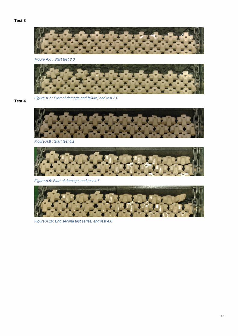
48

Figure A.6 : Start test 3.0

Figure A.7 : Start of damage and failure, end test 3.0

Figure A.8 : Start test 4.2

Figure A.9: Start of damage, end test 4.7

Figure A.10: End second test series, end test 4.8

Test 3

Test 4

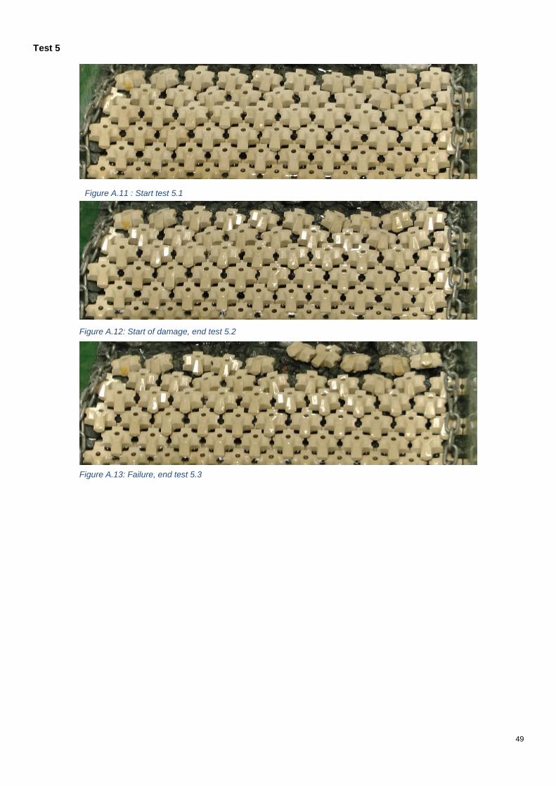
49

Figure A.11 : Start test 5.1

Figure A.12: Start of damage, end test 5.2

Figure A.13: Failure, end test 5.3

Test 5

Test Backfill Wave % Hmo [m] Rc [m] Sop L0 [m] Tp [s] Rc/Hmo h_toe [m] t_test [min]

t_test [sec]

h_paddle [m]

1,1 None 60 0,057 0,095 0,04 1,425 0,96 1,67 0,16 15,93 955,75 0,485

1,2 None 80 0,076 0,095 0,04 1,9 1,10 1,25 0,16 18,39 1103,61 0,485

1,3 None 100 0,095 0,095 0,04 2,375 1,23 1,00 0,16 20,56 1233,87 0,485

1,4 None 110 0,1045 0,095 0,04 2,6125 1,29 0,91 0,16 21,57 1294,09 0,485

1,5 None 120 0,114 0,095 0,04 2,85 1,35 0,83 0,16 22,53 1351,64 0,485

1,6 None 130 0,1235 0,095 0,04 3,0875 1,41 0,77 0,16 23,45 1406,83 0,485

1,7 None 140 0,133 0,095 0,04 3,325 1,46 0,71 0,16 24,33 1459,94 0,485

1,8 None 150 0,1425 0,095 0,04 3,5625 1,51 0,67 0,16 25,19 1511,18 0,485

2,1 None 60 0,057 0,048 0,04 1,425 0,96 0,84 0,207 15,93 955,75 0,532

2,2 None 80 0,076 0,048 0,04 1,9 1,10 0,63 0,207 18,39 1103,61 0,532

2,3 None 100 0,095 0,048 0,04 2,375 1,23 0,51 0,207 20,56 1233,87 0,532

2,4 None 110 0,1045 0,048 0,04 2,6125 1,29 0,46 0,207 21,57 1294,09 0,532

2,5 None 120 0,114 0,048 0,04 2,85 1,35 0,42 0,207 22,53 1351,64 0,532

2,6 None 130 0,1235 0,048 0,04 3,0875 1,41 0,39 0,207 23,45 1406,83 0,532

3 None 53 0,05 0 0,04 1,25 0,90 0,00 0,255 14,92 895,14 0,585

3,1 None 60 0,057 0 0,04 1,425 0,96 0,00 0,255 15,93 955,75 0,585

3,2 None 80 0,076 0 0,04 1,9 1,10 0,00 0,255 18,39 1103,61 0,585

3,3 None 100 0,095 0 0,04 2,375 1,23 0,00 0,255 20,56 1233,87 0,585

3,4 None 110 0,1045 0 0,04 2,6125 1,29 0,00 0,255 21,57 1294,09 0,585

3,5 None 120 0,114 0 0,04 2,85 1,35 0,00 0,255 22,53 1351,64 0,585

3,7 None 140 0,133 0 0,04 3,325 1,46 0,00 0,255 24,33 1459,94 0,585

4,2 Stiff 80 0,076 0,048 0,04 1,9 1,10 0,63 0,207 18,39 1103,61 0,532

4,3 Stiff 100 0,095 0,048 0,04 2,375 1,23 0,51 0,207 20,56 1233,87 0,532

4,5 Stiff 120 0,114 0,048 0,04 2,85 1,35 0,42 0,207 22,53 1351,64 0,532

4,7 Stiff 140 0,133 0,048 0,04 3,325 1,46 0,36 0,207 24,33 1459,94 0,532

4,8 Stiff 150 0,1425 0,048 0,04 3,5625 1,51 0,34 0,207 25,19 1511,18 0,532

5,1 xbloc+ 60 0,057 0,048 0,04 1,425 0,96 0,84 0,207 15,93 955,75 0,532

5,2 xbloc+ 80 0,076 0,048 0,04 1,9 1,10 0,63 0,207 18,39 1103,61 0,532

5,3 xbloc+ 100 0,095 0,048 0,04 2,375 1,23 0,51 0,207 20,56 1233,87 0,532

5,5 xbloc+ 120 0,114 0,048 0,04 2,85 1,35 0,42 0,207 22,53 1351,64 0,532

Table A.1.: Theoretical generated wave parameters

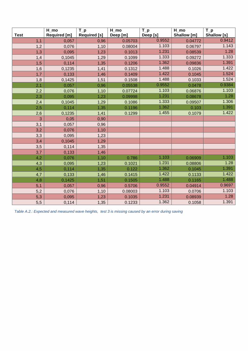
Test H_mo Required [m]

T_p Required [s]

H_mo Deep [m]

T_p Deep [s]

H_mo Shallow [m]

T_p Shallow [s]

1,1 0,057 0,96 0.05703 0.9552 0.04772 0.9412

1,2 0,076 1,10 0.08004 1.103 0.06797 1.143

1,3 0,095 1,23 0.1013 1.231 0.08539 1.28

1,4 0,1045 1,29 0.1099 1.333 0.09272 1.333

1,5 0,114 1,35 0.1206 1.362 0.09836 1.391

1,6 0,1235 1,41 0.1312 1.488 0.1026 1.422

1,7 0,133 1,46 0.1409 1.422 0.1045 1.524

1,8 0,1425 1,51 0.1508 1.488 0.1033 1.524

2,1 0,057 0,96 0.05538 0.9552 0.0478 0.9384

2,2 0,076 1,10 0.07724 1.103 0.06876 1.103

2,3 0,095 1,23 0.09998 1.231 0.08678 1.28

2,4 0,1045 1,29 0.1086 1.333 0.09507 1.306

2,5 0,114 1,35 0.1196 1.362 0.103 1.391

2,6 0,1235 1,41 0.1299 1.455 0.1079 1.422

3 0,05 0,90

3,1 0,057 0,96

3,2 0,076 1,10

3,3 0,095 1,23

3,4 0,1045 1,29

3,5 0,114 1,35

3,7 0,133 1,46

4,2 0,076 1,10 0.786 1.103 0.06909 1.103

4,3 0,095 1,23 0.1021 1.231 0.08806 1.28

4,5 0,114 1,35 0.122 1.362 0.1045 1.391

4,7 0,133 1,46 0.1415 1.422 0.1133 1.422

4,8 0,1425 1,51 0.1505 1.488 0.1165 1.488

5,1 0,057 0,96 0.5706 0.9552 0.04914 0.9697

5,2 0,076 1,10 0.08003 1.103 0.0706 1.103

5,3 0,095 1,23 0.1035 1.231 0.08939 1.28

5,5 0,114 1,35 0.1233 1.362 0.1058 1.391

Table A.2.: Expected and measured wave heights, test 3 is missing caused by an error during saving

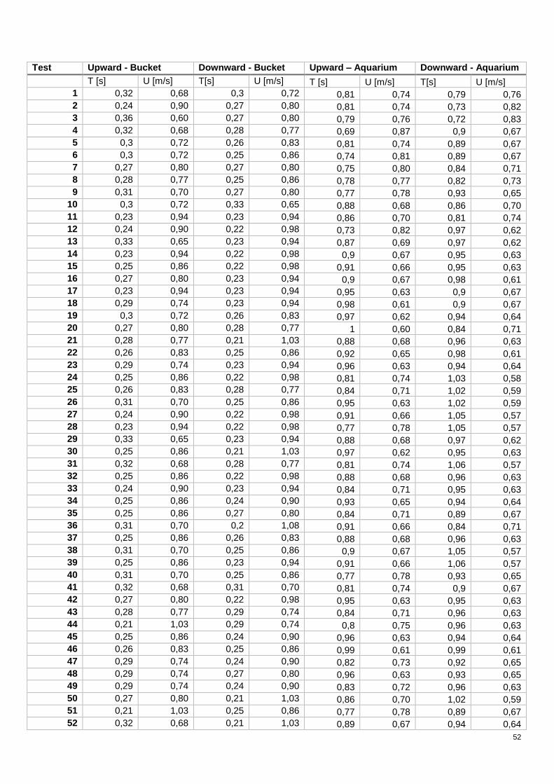
52

Test Upward - Bucket Downward - Bucket Upward – Aquarium Downward - Aquarium

T [s] U [m/s] T[s] U [m/s] T [s] U [m/s] T[s] U [m/s]

1 0,32 0,68 0,3 0,72 0,81 0,74 0,79 0,76

2 0,24 0,90 0,27 0,80 0,81 0,74 0,73 0,82

3 0,36 0,60 0,27 0,80 0,79 0,76 0,72 0,83

4 0,32 0,68 0,28 0,77 0,69 0,87 0,9 0,67

5 0,3 0,72 0,26 0,83 0,81 0,74 0,89 0,67

6 0,3 0,72 0,25 0,86 0,74 0,81 0,89 0,67

7 0,27 0,80 0,27 0,80 0,75 0,80 0,84 0,71

8 0,28 0,77 0,25 0,86 0,78 0,77 0,82 0,73

9 0,31 0,70 0,27 0,80 0,77 0,78 0,93 0,65

10 0,3 0,72 0,33 0,65 0,88 0,68 0,86 0,70

11 0,23 0,94 0,23 0,94 0,86 0,70 0,81 0,74

12 0,24 0,90 0,22 0,98 0,73 0,82 0,97 0,62

13 0,33 0,65 0,23 0,94 0,87 0,69 0,97 0,62

14 0,23 0,94 0,22 0,98 0,9 0,67 0,95 0,63

15 0,25 0,86 0,22 0,98 0,91 0,66 0,95 0,63

16 0,27 0,80 0,23 0,94 0,9 0,67 0,98 0,61

17 0,23 0,94 0,23 0,94 0,95 0,63 0,9 0,67

18 0,29 0,74 0,23 0,94 0,98 0,61 0,9 0,67

19 0,3 0,72 0,26 0,83 0,97 0,62 0,94 0,64

20 0,27 0,80 0,28 0,77 1 0,60 0,84 0,71

21 0,28 0,77 0,21 1,03 0,88 0,68 0,96 0,63

22 0,26 0,83 0,25 0,86 0,92 0,65 0,98 0,61

23 0,29 0,74 0,23 0,94 0,96 0,63 0,94 0,64

24 0,25 0,86 0,22 0,98 0,81 0,74 1,03 0,58

25 0,26 0,83 0,28 0,77 0,84 0,71 1,02 0,59

26 0,31 0,70 0,25 0,86 0,95 0,63 1,02 0,59

27 0,24 0,90 0,22 0,98 0,91 0,66 1,05 0,57

28 0,23 0,94 0,22 0,98 0,77 0,78 1,05 0,57

29 0,33 0,65 0,23 0,94 0,88 0,68 0,97 0,62

30 0,25 0,86 0,21 1,03 0,97 0,62 0,95 0,63

31 0,32 0,68 0,28 0,77 0,81 0,74 1,06 0,57

32 0,25 0,86 0,22 0,98 0,88 0,68 0,96 0,63

33 0,24 0,90 0,23 0,94 0,84 0,71 0,95 0,63

34 0,25 0,86 0,24 0,90 0,93 0,65 0,94 0,64

35 0,25 0,86 0,27 0,80 0,84 0,71 0,89 0,67

36 0,31 0,70 0,2 1,08 0,91 0,66 0,84 0,71

37 0,25 0,86 0,26 0,83 0,88 0,68 0,96 0,63

38 0,31 0,70 0,25 0,86 0,9 0,67 1,05 0,57

39 0,25 0,86 0,23 0,94 0,91 0,66 1,06 0,57

40 0,31 0,70 0,25 0,86 0,77 0,78 0,93 0,65

41 0,32 0,68 0,31 0,70 0,81 0,74 0,9 0,67

42 0,27 0,80 0,22 0,98 0,95 0,63 0,95 0,63

43 0,28 0,77 0,29 0,74 0,84 0,71 0,96 0,63

44 0,21 1,03 0,29 0,74 0,8 0,75 0,96 0,63

45 0,25 0,86 0,24 0,90 0,96 0,63 0,94 0,64

46 0,26 0,83 0,25 0,86 0,99 0,61 0,99 0,61

47 0,29 0,74 0,24 0,90 0,82 0,73 0,92 0,65

48 0,29 0,74 0,27 0,80 0,96 0,63 0,93 0,65

49 0,29 0,74 0,24 0,90 0,83 0,72 0,96 0,63

50 0,27 0,80 0,21 1,03 0,86 0,70 1,02 0,59

51 0,21 1,03 0,25 0,86 0,77 0,78 0,89 0,67

52 0,32 0,68 0,21 1,03 0,89 0,67 0,94 0,64

53

53 0,25 0,86 0,28 0,77 0,95 0,63 0,92 0,65

54 0,26 0,83 0,22 0,98 0,96 0,63 0,95 0,63

55 0,28 0,77 0,21 1,03 0,96 0,63 0,84 0,71

56 0,25 0,86 0,27 0,80 0,9 0,67 0,9 0,67

57 0,34 0,64 0,21 1,03 0,95 0,63 0,89 0,67

58 0,25 0,86 0,22 0,98 0,86 0,70 0,9 0,67

59 0,31 0,70 0,25 0,86 0,94 0,64 0,84 0,71

60 0,26 0,83 0,23 0,94 0,88 0,68 0,85 0,71

61 0,22 0,98 0,24 0,90 0,91 0,66 0,86 0,70

62 0,33 0,65 0,24 0,90 0,92 0,65 0,86 0,70

63 0,24 0,90 0,25 0,86 0,91 0,66 0,88 0,68

64 0,28 0,77 0,23 0,94 0,91 0,66 0,95 0,63

65 0,21 1,03 0,23 0,94 0,92 0,65 0,84 0,71

66 0,25 0,86 0,24 0,90 0,92 0,65 0,82 0,73

67 0,23 0,94 0,24 0,90 0,89 0,67 0,91 0,66

68 0,25 0,86 0,25 0,86 0,91 0,66 0,91 0,66

69 0,31 0,70 0,26 0,83 0,93 0,65 0,9 0,67

70 0,21 1,03 0,28 0,77 0,93 0,65 0,97 0,62

71 0,28 0,77 0,23 0,94 0,95 0,63 1,01 0,59

72 0,31 0,70 0,25 0,86 0,99 0,61 0,93 0,65

73 0,3 0,72 0,23 0,94 0,93 0,65 0,97 0,62

74 0,23 0,94 0,22 0,98 0,85 0,71 0,96 0,63

75 0,33 0,65 0,28 0,77 0,93 0,65 0,89 0,67

76 0,33 0,65 0,24 0,90 1,03 0,58 0,98 0,61

77 0,21 1,03 0,27 0,80 0,88 0,68 0,92 0,65

78 0,26 0,83 0,24 0,90 0,99 0,61 0,87 0,69

79 0,28 0,77 0,21 1,03 0,88 0,68 0,94 0,64

80 0,25 0,86 0,22 0,98 0,95 0,63 0,95 0,63

81 0,28 0,77 0,22 0,98 0,89 0,67 0,93 0,65

82 0,22 0,98 0,26 0,83 0,86 0,70 0,94 0,64

83 0,24 0,90 0,25 0,86 0,78 0,77 0,98 0,61

84 0,23 0,94 0,26 0,83 0,99 0,61 0,91 0,66

85 0,22 0,98 0,26 0,83 0,84 0,71 0,86 0,70

86 0,3 0,72 0,23 0,94 0,95 0,63 0,83 0,72

87 0,28 0,77 0,29 0,74 0,84 0,71 0,89 0,67

88 0,24 0,90 0,24 0,90 0,9 0,67 0,86 0,70

89 0,27 0,80 0,21 1,03 0,88 0,68 0,85 0,71

90 0,3 0,72 0,27 0,80 0,9 0,67 1 0,60

91 0,25 0,86 0,26 0,83 0,84 0,71 0,97 0,62

92 0,32 0,68 0,23 0,94 0,93 0,65 0,91 0,66

93 0,23 0,94 0,25 0,86 0,96 0,63 0,94 0,64

94 0,23 0,94 0,25 0,86 0,79 0,76 0,96 0,63

95 0,25 0,86 0,2 1,08 0,93 0,65 0,9 0,67

96 0,28 0,77 0,24 0,90 0,84 0,71 1,02 0,59

97 0,27 0,80 0,26 0,83 0,8 0,75 0,93 0,65

98 0,25 0,86 0,26 0,83 0,86 0,70 0,89 0,67

99 0,26 0,83 0,23 0,94 0,89 0,67 1,02 0,59

100 0,25 0,86 0,25 0,86 0,9 0,67 0,89 0,67

Average 0,2702 0,80 0,2453 0,88 0,88 0,68 0,92 0,65

Stdev 0,03519 0,025324 0,068819 0,066505

95% interval

T –Bucket up [s] T –Bucket down [s] T –Aquarium up [s] T –Aquarium down [s]

0,263303 0,277097 0,240336 0,250264 0,870912 0,897888 0,911365 0,937435 Table A.3.: Results fall tests bucket and aquarium

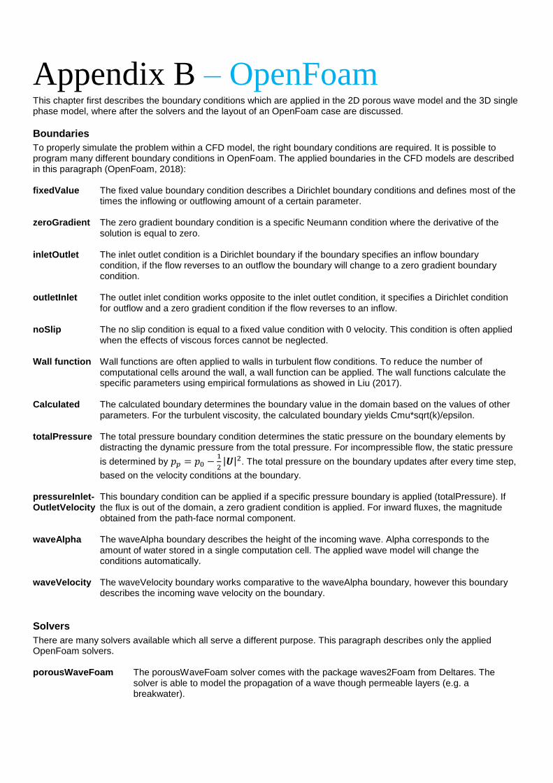
Appendix B – OpenFoam This chapter first describes the boundary conditions which are applied in the 2D porous wave model and the 3D single phase model, where after the solvers and the layout of an OpenFoam case are discussed.

Boundaries

To properly simulate the problem within a CFD model, the right boundary conditions are required. It is possible to program many different boundary conditions in OpenFoam. The applied boundaries in the CFD models are described in this paragraph (OpenFoam, 2018): fixedValue The fixed value boundary condition describes a Dirichlet boundary conditions and defines most of the

times the inflowing or outflowing amount of a certain parameter. zeroGradient The zero gradient boundary condition is a specific Neumann condition where the derivative of the

solution is equal to zero. inletOutlet The inlet outlet condition is a Dirichlet boundary if the boundary specifies an inflow boundary

condition, if the flow reverses to an outflow the boundary will change to a zero gradient boundary condition.

outletInlet The outlet inlet condition works opposite to the inlet outlet condition, it specifies a Dirichlet condition

for outflow and a zero gradient condition if the flow reverses to an inflow.

noSlip The no slip condition is equal to a fixed value condition with 0 velocity. This condition is often applied when the effects of viscous forces cannot be neglected.

Wall function Wall functions are often applied to walls in turbulent flow conditions. To reduce the number of

computational cells around the wall, a wall function can be applied. The wall functions calculate the specific parameters using empirical formulations as showed in Liu (2017).

Calculated The calculated boundary determines the boundary value in the domain based on the values of other

parameters. For the turbulent viscosity, the calculated boundary yields Cmu*sqrt(k)/epsilon. totalPressure The total pressure boundary condition determines the static pressure on the boundary elements by

distracting the dynamic pressure from the total pressure. For incompressible flow, the static pressure

is determined by 𝑝𝑝 = 𝑝0 −1

2|𝑼|2. The total pressure on the boundary updates after every time step,

based on the velocity conditions at the boundary. pressureInlet- This boundary condition can be applied if a specific pressure boundary is applied (totalPressure). If OutletVelocity the flux is out of the domain, a zero gradient condition is applied. For inward fluxes, the magnitude obtained from the path-face normal component. waveAlpha The waveAlpha boundary describes the height of the incoming wave. Alpha corresponds to the

amount of water stored in a single computation cell. The applied wave model will change the conditions automatically.

waveVelocity The waveVelocity boundary works comparative to the waveAlpha boundary, however this boundary

describes the incoming wave velocity on the boundary.

Solvers

There are many solvers available which all serve a different purpose. This paragraph describes only the applied OpenFoam solvers. porousWaveFoam The porousWaveFoam solver comes with the package waves2Foam from Deltares. The

solver is able to model the propagation of a wave though permeable layers (e.g. a breakwater).

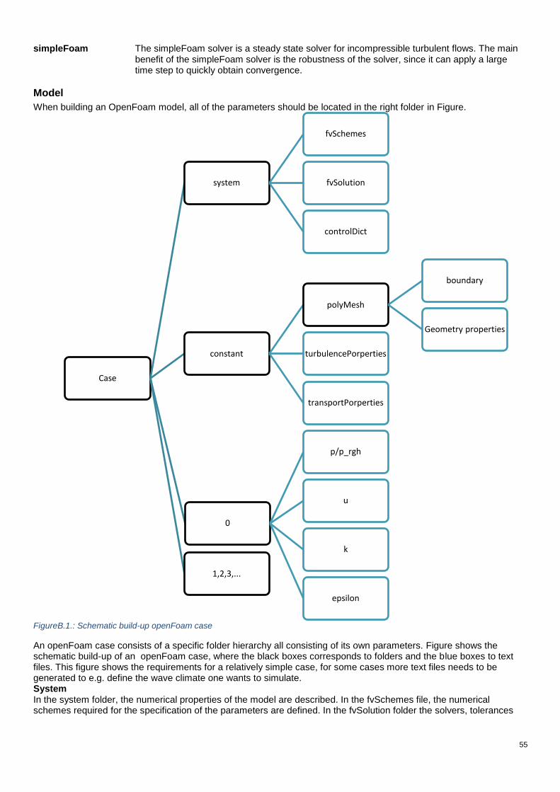
55

simpleFoam The simpleFoam solver is a steady state solver for incompressible turbulent flows. The main benefit of the simpleFoam solver is the robustness of the solver, since it can apply a large time step to quickly obtain convergence.

Model

When building an OpenFoam model, all of the parameters should be located in the right folder in Figure.

FigureB.1.: Schematic build-up openFoam case

An openFoam case consists of a specific folder hierarchy all consisting of its own parameters. Figure shows the schematic build-up of an openFoam case, where the black boxes corresponds to folders and the blue boxes to text files. This figure shows the requirements for a relatively simple case, for some cases more text files needs to be generated to e.g. define the wave climate one wants to simulate. System In the system folder, the numerical properties of the model are described. In the fvSchemes file, the numerical schemes required for the specification of the parameters are defined. In the fvSolution folder the solvers, tolerances

Case

system

fvSchemes

fvSolution

controlDict

constant

polyMesh

boundary

Geometry properties

turbulencePorperties

transportPorperties

0

p/p_rgh

u

k

epsilon

1,2,3,...

56

and algorithms are controlled. The controlDict defines the timestep, the total run time and the data processing of the model. Constant The constant folder defines the physical properties of the model. In the polyMesh folder, the geometrical parameters are defined, such as the location of the faces, the mesh spacing and the definition of the boundary faces (whether the boundary behaves as an patch, wall or an empty field). In the turbulencePorperties file one defines whether the flow is laminar or turbulent. If a turbulent system is chosen, the closure model has to be selected as well. The transportProperties file defines whether the fluid is compressible and defines the viscosity of the fluid or air. 0 In the 0 folder, the initial conditions and the boundary conditions are defined. This is done for each calculated parameter individually. The folders with a higher number than 0 serve as an output of the model and will automatically be created during a simulation, based on the writeControl definition in the controlDict file.

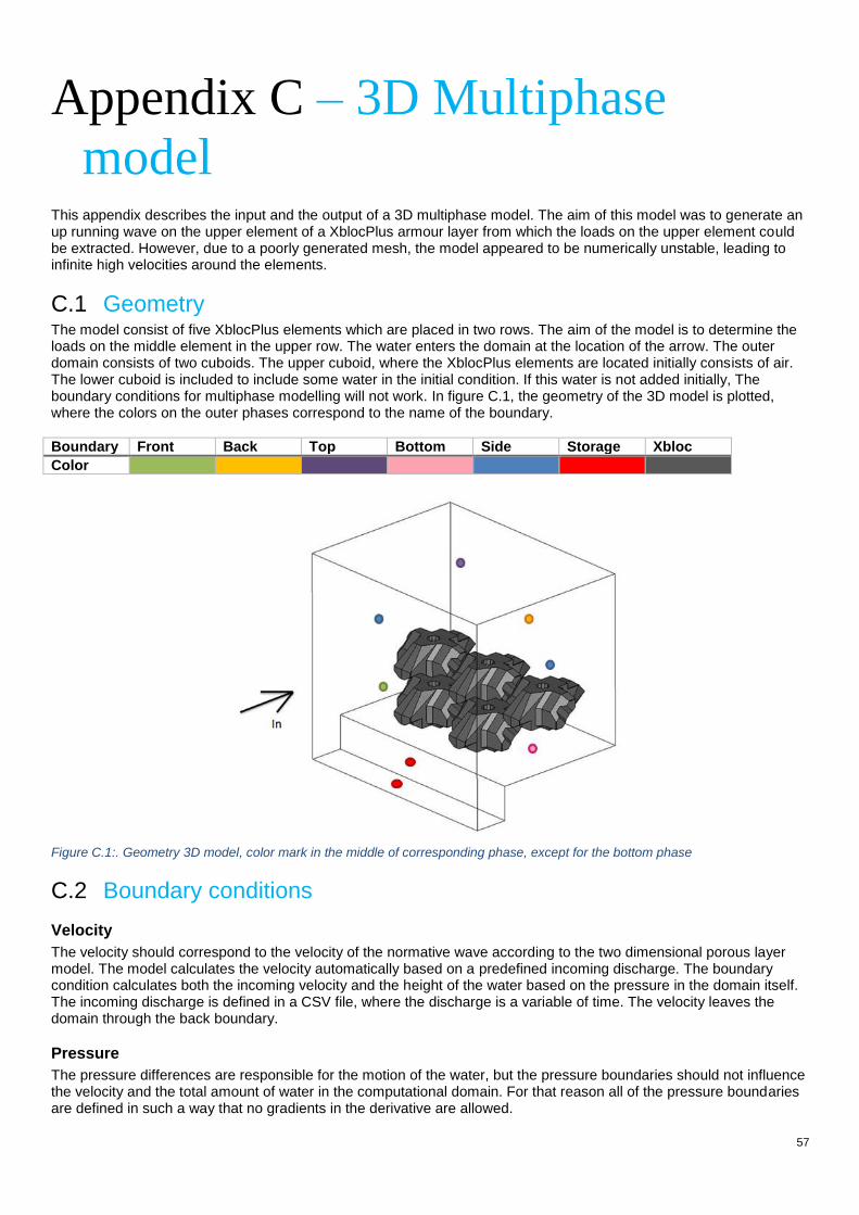
57

Appendix C – 3D Multiphase

model This appendix describes the input and the output of a 3D multiphase model. The aim of this model was to generate an up running wave on the upper element of a XblocPlus armour layer from which the loads on the upper element could be extracted. However, due to a poorly generated mesh, the model appeared to be numerically unstable, leading to infinite high velocities around the elements.

C.1 Geometry The model consist of five XblocPlus elements which are placed in two rows. The aim of the model is to determine the loads on the middle element in the upper row. The water enters the domain at the location of the arrow. The outer domain consists of two cuboids. The upper cuboid, where the XblocPlus elements are located initially consists of air. The lower cuboid is included to include some water in the initial condition. If this water is not added initially, The boundary conditions for multiphase modelling will not work. In figure C.1, the geometry of the 3D model is plotted, where the colors on the outer phases correspond to the name of the boundary.

Boundary Front Back Top Bottom Side Storage Xbloc

Color

Figure C.1:. Geometry 3D model, color mark in the middle of corresponding phase, except for the bottom phase

C.2 Boundary conditions

Velocity

The velocity should correspond to the velocity of the normative wave according to the two dimensional porous layer model. The model calculates the velocity automatically based on a predefined incoming discharge. The boundary condition calculates both the incoming velocity and the height of the water based on the pressure in the domain itself. The incoming discharge is defined in a CSV file, where the discharge is a variable of time. The velocity leaves the domain through the back boundary.

Pressure

The pressure differences are responsible for the motion of the water, but the pressure boundaries should not influence the velocity and the total amount of water in the computational domain. For that reason all of the pressure boundaries are defined in such a way that no gradients in the derivative are allowed.

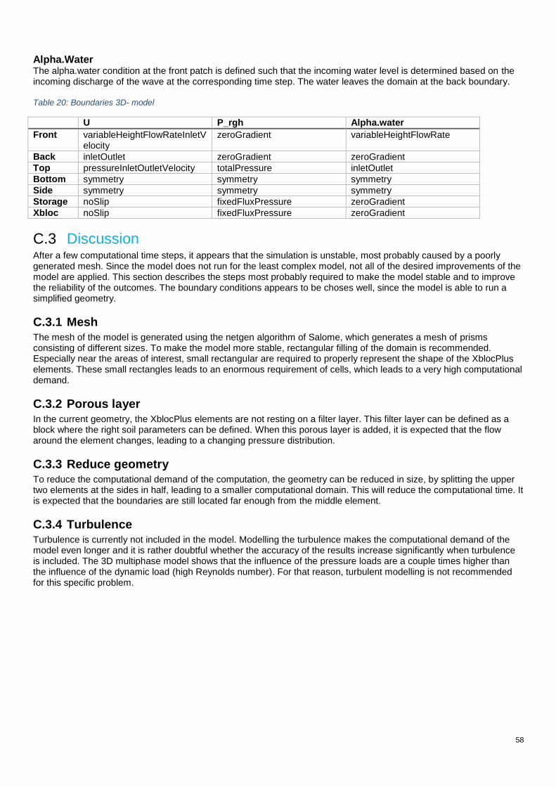
58

Alpha.Water The alpha.water condition at the front patch is defined such that the incoming water level is determined based on the incoming discharge of the wave at the corresponding time step. The water leaves the domain at the back boundary. Table 20: Boundaries 3D- model

U P_rgh Alpha.water

Front variableHeightFlowRateInletVelocity

zeroGradient variableHeightFlowRate

Back inletOutlet zeroGradient zeroGradient

Top pressureInletOutletVelocity totalPressure inletOutlet

Bottom symmetry symmetry symmetry

Side symmetry symmetry symmetry

Storage noSlip fixedFluxPressure zeroGradient

Xbloc noSlip fixedFluxPressure zeroGradient

C.3 Discussion After a few computational time steps, it appears that the simulation is unstable, most probably caused by a poorly generated mesh. Since the model does not run for the least complex model, not all of the desired improvements of the model are applied. This section describes the steps most probably required to make the model stable and to improve the reliability of the outcomes. The boundary conditions appears to be choses well, since the model is able to run a simplified geometry.

C.3.1 Mesh

The mesh of the model is generated using the netgen algorithm of Salome, which generates a mesh of prisms consisting of different sizes. To make the model more stable, rectangular filling of the domain is recommended. Especially near the areas of interest, small rectangular are required to properly represent the shape of the XblocPlus elements. These small rectangles leads to an enormous requirement of cells, which leads to a very high computational demand.

C.3.2 Porous layer

In the current geometry, the XblocPlus elements are not resting on a filter layer. This filter layer can be defined as a block where the right soil parameters can be defined. When this porous layer is added, it is expected that the flow around the element changes, leading to a changing pressure distribution.

C.3.3 Reduce geometry

To reduce the computational demand of the computation, the geometry can be reduced in size, by splitting the upper two elements at the sides in half, leading to a smaller computational domain. This will reduce the computational time. It is expected that the boundaries are still located far enough from the middle element.

C.3.4 Turbulence

Turbulence is currently not included in the model. Modelling the turbulence makes the computational demand of the model even longer and it is rather doubtful whether the accuracy of the results increase significantly when turbulence is included. The 3D multiphase model shows that the influence of the pressure loads are a couple times higher than the influence of the dynamic load (high Reynolds number). For that reason, turbulent modelling is not recommended for this specific problem.