D. Geskus

Design and construction ofregenerative amplifier andcompressor for chirpedpulse amplification

D. Geskus

Design and construction ofregenerative amplifier andcompressor for chirpedpulse amplification

University of Twente

Department of Science and Technology

Laser Physics and Non-linear Optics

Enschede, July 11, 2006

Graduation Committee:

Prof. Dr. K.J. Boller

Dr. Ir. F.A. van Goor

Prof. Dr. M. Pollnau

Dr. H.J.W.M. Hoekstra

Summary

Research on acceleration of electrons by plasma waves will be performed at thelaser physics and non-linear optics group of the University of Twente to developa new compact method for acceleration of electrons. This method of electronacceleration requires an intense ultrashort laser pulse to induce a plasma wavein the plasma on which the electrons can ”surf” to higher kinetic energies.Therefore, a laser is being developed that should deliver an 1 Joule laser pulsewith a duration of 30 fs to generate the demanded 30 TW of optical power forcreation of the plasma wave as required for this electron wake field accelerationexperiment.The principle of the laser is based on chirped pulse amplification; a stretchedpulse is amplified to the demanded energy, and re-compressed afterwards.This report describes the performed work concerning the design and construc-tion of a pre-amplifier and a compressor. For pre-amplification of the pulse aregenerative amplifier is used, which has been constructed and characterised.The measured output power of the regenerative amplifier is approximately 3.5mJ, in the future this pulse will be further amplified by two additional multi-pass amplifiers. But as this further amplification is beyond the scope of thismaster thesis, it will not be treated in this report. A grating compressor withan efficiency of approximately 70%, recompresses the pre-amplified pulse to aduration of 29 fs with a pulse energy of the compressed pulse of 2.5 mJ.For creation of short pulses the dispersion of the optical system becomes veryimportant. Because chirped pulse amplification is based on introducing disper-sion in a controlled manner, it is of vital importance to fully comprehend thesedispersive properties of the experimental set-up. Therefore, mathematical mod-els have been successfully evaluated and the final output of the experimentalset-up agrees very well to the results of the used mathematical models.

3

CONTENTS

Preface 6

1 Introduction 7

1.1 The laser physics group . . . . . . . . . . . . . . . . . . . . . . . 71.2 Acceleration of electrons . . . . . . . . . . . . . . . . . . . . . . . 71.3 Plasma . . . . . . . . . . . . . . . . . . . . . . . . . . . . . . . . . 81.4 University of Twente and the laser wake field acceleration demon-

stration experiment . . . . . . . . . . . . . . . . . . . . . . . . . . 9

2 Laser system 10

2.1 Kerr lens modelocked laser . . . . . . . . . . . . . . . . . . . . . 112.2 Stretcher . . . . . . . . . . . . . . . . . . . . . . . . . . . . . . . 132.3 Regenerative amplifier . . . . . . . . . . . . . . . . . . . . . . . . 152.4 Multi pass amplifier . . . . . . . . . . . . . . . . . . . . . . . . . 172.5 Grating compressor . . . . . . . . . . . . . . . . . . . . . . . . . . 182.6 Grenouille . . . . . . . . . . . . . . . . . . . . . . . . . . . . . . . 18

3 Pulse amplification in detail 22

3.1 Bandwidth of the regenerative amplifier . . . . . . . . . . . . . . 223.2 Analysis of beam propagation . . . . . . . . . . . . . . . . . . . . 26

3.2.1 Calculation of the beam properties by the resonator prop-erties . . . . . . . . . . . . . . . . . . . . . . . . . . . . . 26

3.2.2 Calculation of the beam properties with use of the (ABCD)-Matrix . . . . . . . . . . . . . . . . . . . . . . . . . . . . . 27

3.2.3 Measurements on the waist . . . . . . . . . . . . . . . . . 283.2.4 Results of measurements on waist compared to theoretical

values . . . . . . . . . . . . . . . . . . . . . . . . . . . . . 29

4 Compensation of dispersion 32

4.1 Introduction . . . . . . . . . . . . . . . . . . . . . . . . . . . . . . 324.2 Dispersion compensation . . . . . . . . . . . . . . . . . . . . . . . 36

4.2.1 Inventory of the dispersive elements in the set up . . . . . 374.2.2 Creation of the Maple model with the gathered data . . . 39

4

4.2.3 Find the optimal settings . . . . . . . . . . . . . . . . . . 39

5 Comparison of mathematical models and experiments concern-

ing dispersion 43

5.1 Comparison of the models in the most ideal situation . . . . . . . 435.2 Comparison of the mathematical models to the experiment . . . 475.3 Determination for regen roundtrips . . . . . . . . . . . . . . . . . 485.4 Modelling of the set-up according to the experimental settings . . 495.5 Conclusions concerning the comparison between the mathemati-

cal models and the experimental results . . . . . . . . . . . . . . 50

6 Measurement of the output pulse 53

6.1 Calibration of the Grenouille . . . . . . . . . . . . . . . . . . . . 536.2 Measured output pulse . . . . . . . . . . . . . . . . . . . . . . . . 56

7 Conclusions 57

7.1 Regenerative amplifier . . . . . . . . . . . . . . . . . . . . . . . . 577.2 Mathematical model for dispersion . . . . . . . . . . . . . . . . . 577.3 Re-compression of the pulse . . . . . . . . . . . . . . . . . . . . . 57

8 Recommendations 59

8.1 Regenerative amplifier . . . . . . . . . . . . . . . . . . . . . . . . 598.2 Mathematical model for dispersion . . . . . . . . . . . . . . . . . 608.3 Re-compression of the pulse . . . . . . . . . . . . . . . . . . . . . 60

Bibliography 61

A Schematic of experimental set up 63

B Additional CD 64

5

Preface

The assignment of this masters thesis, was to design and construct a laser thatgenerates an ultrashort laser pulse, and in case of sufficient available time, itwould be an option to shoot the laser pulse at some material and measure theinfluences of this material on the properties of the pulse. But with experimentalphysics one has to rely on the used machines, in this case only three devicesneeded some unforeseen attention. It started with performing maintenance onthe pump laser for the regenerative amplifier. After this laser had been serviced,the power supply of another pump laser started to generate errors. Fortunatelythis occurred not all the time, and did not cause large delay in the develop-ment of the experiment. After construction of the regenerative amplifier, thecompressor had to be designed. During the construction of the compressor, itappeared that the grating surfaces were severely contaminated. After at leastone month I succeeded to find a method to clean them again. During that monthI started to characterise the output of the regenerative amplifier. These actionswhere aborted abruptly once the gratings were clean again and construction ofthe compressor could be started.This introduction shows that the time balance of working with ultrashort lasertechniques is not the most efficient one; after months of construction, the systemoperates for only a few femtoseconds. Fortunately this balance has been fullycompensated by the nice atmosphere at the laser physics group. All the groupmembers add their brick to this sphere, and I want to thank them all for beingmy colleagues. Some of these colleagues among them have to be mentionedmore explicit, like Rolf Loch and Arie Irman, as I had many clarifying discus-sions about every day life and laser physics. And last but not least, I would liketo thank Fred van Goor who patiently learned me how to treat delicate optics,and did not loose the confidence in my work, after peeling off the coating fromone of the gratings.

Enschede, July 11, 2006

Dimitri Geskus

6

CHAPTER 1

Introduction

1.1 The laser physics group

The research of the laser physics group at the University of Twente is focussedon experiments using the special properties of laser light. Light produced bylasers can have many special properties like coherence, colour, intensity, andshape of pulse. Lasers, as we know them now, started their developments only50 years ago. Though novel developments in the laser regime occur daily. Thishas enlarged the field of research enormously, so that now many research groupsuse lasers to perform their experiments. The laser physics group develops spe-cial lasers, in order to exploit their use in new regions of research. In thismanner new theories can be proved, and fascinating non-linear effects can thusbe demonstrated.

1.2 Acceleration of electrons

Particle accelerators are developed for use in many research fields. Still a largefield has to be explored in this field of high energy physics, but progress is slowdue to the costs of these machines. CERN for example has one giant accelerator,which is 27 km in circumference, making it a very expensive machine. Thesemachines are that large, due to the fact that the particles have to be acceleratedby an electric field. This field is generated with super conductive RF resonatorsand the maximum field that these machines nowadays can produce is 46 MV/m[1]. Acceleration of electrons with this type of accelerator to a modest energy of20 GeV, requires an accelerator length of 20G/46M=435 meters. As this showsthe reason for the large dimensions of these machines it is clear that we needstronger electric fields, in order to shrink the dimensions of these accelerators. Aplace where high electric fields can be found is in the core of atoms. A hydrogenatom for example has an electric field of E = e/(4πε0a

20) ≈ 5 GV cm−1, where

e = 1.6 · 10−19C (electron charge), ε0 = 8.85 · 10−12Fm−1 (electric permittivityof vacuum) and a0 = 5.29 · 10−11m (Bohr radius). An accelerator with theseelectric fields would need only 4 centimetre to accelerate particles to energies

7

of 20 GeV. To access these fields a laser pulse is used to separate the electronsfrom the core. This can be performed in a plasma.

1.3 Plasma

Plasma is also called the fourth state of matter, besides solid, liquid and gas. Ina plasma state the electrons are not bound to the residual core; the atoms of thematerial are ionised. There are many degrees of ionisation, and the easiest caseis that of the hydrogen atom. When a hydrogen atom gets ionised, only oneproton remains, and a free electron is created. When the matter is in completeplasma state all the atoms are completely ionised, creating a cloud of chargedparticles. The plasma has no nett charge, because the electrons and the atomcores are equally distributed due to electric interaction of the particles cancel outthe electric fields. This balance of electron and ion density can be disturbed by alaser pulse. A strong laser pulse scatters the electrons in all directions due to socalled ponderomotive forces, while as the position of the ions remains unchangedfor a small time scale due to their larger masses. As a result a positive chargedregion remains. After the pulse has passed this region, the electrons will returnto their original position driven by the generated electric field. Due to thisimplosion of the electrons an excess of electrons is generated after some time,so that the electrons will be scattered again, creating an oscillating potentialfield. As the laser pulse passes through the plasma, a potential wave will becreated in the plasma, much like when one is walking through the wardrobe,and touching all the coat hangers when passing by. The result, shown in figure

25 20 15 10 5 00.4

0.2

0

0.2

0.4

0.6

laser field

longitudinal field

z

Decelerating if Ez > 0

Accelerating if Ez < 0electron

lp

25 20 15 10 5 00.4

0.2

0

0.2

0.4

0.6

laser field

longitudinal field

z

Decelerating if Ez > 0

Accelerating if Ez < 0electron

lp

Figure 1.1: Plasma wakefield

1.1, is a travelling wave with a phase speed equal to the group velocity of thelaser pulse. Injection of electrons at the right moment in this plasma wave withthe same velocity of the laser pulse will let the electrons experience an electric

8

field in the propagation direction. This principle is better known as electronwake field acceleration. More details about plasma based particle acceleratorscan be found in [2].

1.4 University of Twente and the laser wake field

acceleration demonstration experiment

In the laser wake field acceleration experiment, relativistic electrons will befurther accelerated by a plasma wave which is induced by an ultra short laserpulse. Therefore it requires a harmonic symbioses of the following three physicalaspects:

• Beam of relativistic electrons

• Ultra short, high energetic laser pulse, which is partly described in thisreport

• Plasma channel

It is an impossible task to develop these three fields simultaneous at a singleinstitute. Therefore a collaboration between three institutes in the Netherlandsshare their expertises in this project. The cooperative institutes are:

• Laser Physics and Non-linear Optics group of the University of Twente,providing the 30 TW laser.

• FOM-Institute for Plasma Physics Rijnhuizen, Laser-Plasma XUV Sourceand XUV optics group, investing the plasma channel.

• Physics and Applications of Ion Beams and Accelerators group of theUniversity of Eindhoven, providing the electron beam.

Together all the required physical aspects are covered, and each of the instituteshas to develop their part to combine it into the project. But during the first yearsof this project things developed into different directions, and new ideas have beencreated at the University of Twente. These new ideas concern novel injectionscheme of the electrons in the wake field [4] [5]. Now another project has startedat the University of Twente. This parallel project concerns the construction ofthe complete experiment at the University of Twente. Fortunately the facilitiesof University of Twente cover all the demanded equipment for the experiment.An RF electron accelerator is leftover from a former free electron laser (FEL)project. The laser for the ultra short pulse is in any case under construction forthe main project, only the plasma channel has to be developed from scratch. Inthe meanwhile the cooperation with the other institutes remains, not only forthe initial project but also for the re-adjustments concerning the electron beam,and the development of the plasma channel. The demonstration experiment isstill planned to be performed at the University of Eindhoven, but this is basedon a different electron injection scheme [6].

9

CHAPTER 2

Laser system

Light intensities of several terawatts are required to perform electron wake fieldacceleration for the demonstration experiment at the University of Twente. Thesame intensities can be achieved by focussing all the sunlight that falls onto theearth onto the surface of a pinhead. These intensities are enormous and thereforeit is not possible to generate this amount of light in a continuous manner, ratherit has to be generated in a pulsed manner. The laser system used for this purpose

Polarisation

Polarisation

Output

Oscillator

Regen

Compressor

Stretcher

Figure 2.1: Chirped pulse amplification set up

is a combination of a Kerr-lens mode locked (KLM) laser in combination with achirped pulse amplifier (CPA) system [3]. In this amplifier short pulses of a fewfemtoseconds from the KLM laser are stretched in time to a few hundreds ofpicoseconds, before they are amplified in three stages to two Joules of energy, atthe end they are re-compressed to a few femtoseconds. After re-compression oneJoule of pulse energy and 30 terawatt of optical power should be available, seefigure 2.2. Two types of amplifiers are used in this system, a regenerative pre

10

amplifier and two multipass amplifiers. Further details concerning the choiceof these types of amplifiers in this experiment is discussed in section 2.3. The

Figure 2.2: The pulse from the oscillator will be stretched, amplified and re-compressed to its original duration

following sections will describe the elements of the complete set up in sequenceof the route that the initial pulse will travel through the set up.

2.1 Kerr lens modelocked laser

The initial pulse is generated in a KLM laser. This laser is based on a TiSacrystal, a material that is very suitable for generation and amplification of ultrashort pulses, due to its very broad gain bandwidth of 235 nm around 800 nm [7].The laser resonator, on the contrary, will not support this continuous spectrum,but only a limited number of discrete resonator modi. Resonator modi areintroduced due to the resonator length (l), as most wavelengths will cancelthemselves out by destructive interference after one or more cycles through theresonator cavity, as can been seen in figure 2.3. The frequency separation (4ν)

Allowed mode

Instable mode

Allowed mode

Cavity length (L)

Figure 2.3: Cavity modi

11

between the successive modi is:

4ν =c

2l, (2.1)

with c the velocity of light. Each individual longitudinal mode itself supports asmall bandwidth, but typically this bandwidth is much smaller than the inter-mode frequency separation. Higher order transverse modi are suppressed by thegeometry of the cavity. The combination of cavity length, concave mirrors andthe apertures in the cavity will force the output to single transverse mode. A

Laser gain bandwidth

cavity longitudinal mode structure

Laser output spectrum

Frequency

Dn=c/2L

Ga

inG

ain

Inte

nsi

ty

Figure 2.4: Laser spectrum

normal non-mode-locked laser will start to produce light in all of the supportedlaser modi, but after some roundtrips all energy will be concentrated into a fewlaser modi, namely those with the strongest gain. This reduces the bandwidthof the output light, which is of vital importance for generation of ultra shortpulses. Therefore this effect has to be avoided. Mapping these modi onto thegain bandwidth of the TiSa crystal it is obvious that a large number of modican be generated with this type of laser, shown in figure 2.4. To keep the laserfrom generating light in only a few of its modi, it should be operated in a pulsedmode. In a pulsed laser the modi with the strongest gain will less likely startto dominate the output of the laser, and the power is not concentrated in onefrequency. To let the laser operate in an ultra short pulsed manner the modihave to be locked in a manner that all the modi involved have constructiveinterference at the same moment in time with each other. So in a modelockedlaser all the modi are in phase with each other. The set up described here isbased on Kerr lens mode locking, which is a passive modelocking technique. AKerr-lens is made in material of which the refractive index n is strongly intensitydependent, according n = n0 +n2 · I, with n0 the low intensity refractive index,and n2 the changes of the refractive index as function of the intensity of thelight I. In the experimental set-up the TiSa crystal fulfils this role. When theintensity of the light is not sufficient no lens effect will occur in the material,but at higher intensities lensing effects will occur because the refractive indexwill be higher in centre of the laser pulse, creating a gradient index lens in the

12

material due to the spacial shape of the pulse. When a laser starts to operatein a pulsed mode, the energy will be compressed in time into pulses of highintensity. The average output power does not show large changes, as the pumpenergy remains unchanged. Then it is clear that the Kerr-effect will only occurwhen the laser is operating in pulsed mode, and that the mode-locking effectwill sustain this pulsed mode. As the resonator of the Kerr-lens mode-lockedlaser has been optimised, containing a Kerr-lens, it will be less stable for non-mode-locked CW output. Figure 2.5 shows the Kerr-lens principle with a hardaperture, where a large part of the output in CW mode will be absorbed. In theexperiment a so called soft aperture is created by the focus of the pump-laserin the TiSa crystal. In the KLM laser the material dispersion of one round trip

CW

Pulsed

Aperture

Kerr medium

Intensity

Figure 2.5: hard aperture Kerr-lens mode locking principle

in the laser is compensated by a prism pair placed within the resonator cavity,see figure 2.6. The length of the resonator dominates the repetition rate, in this

Oscillator

TiSa crystal

Prism pairOutput

Figure 2.6: Schematic of Kerr lens modelocked laser

case it is set to a repetition frequency of 81.25 MHz. This value is the 16thharmonic of the RF source that drives the linear accelerator at 1.3 GHz, whichwill be used for synchronisation between the two systems. The pulse duration,after compensation for the last round trip is 25 fs. And typical energy per pulseis 1-3 nJ.

2.2 Stretcher

Amplification of the pulse without stretching it in time will cause damage tothe optics, and the amplification of such a short pulse will be less efficient dueto self phase modulation and self focussing effects in the amplifier. Stretchingof the pulse is performed by an Oeffner stretcher [10][9]. This stretcher designis completely symmetric, so that only symmetrical aberration can appear. Thepresence of two spherical mirrors whose radius of curvature ratio is two and ofopposite sign cancels these aberrations, since all the optics are mirrors. In thisoptical combination, perfect stigmatism is ensured only when the grating is at

13

Figure 2.7: Photograph of stretcher

the common centre of curvature. Unfortunately the stretcher will not stretch thepulse when the grating is exactly positioned in this common centre of curvature,but Cheriaux et al. [9] have shown that the spherical aberrations introduced bythe positioning the grating is away from this centre of curvature is weak enoughnot to affect the pulse shape. As the design is based on curved mirrors it doesnot contribute to any material dispersion. The design of the compressor is moreintuitive, than that of the stretcher. The only difference between these designsis the additional telescope in the design of the stretcher to create an image ofthe first grating behind the second grating. According to the definition of animage, all the path lengths to the image are of equal size. This new image ofthe first grating behind the second grating, creates a ”negative” optical distancebetween the two gratings, and the function of separating the colours in time isinverted compared to the compressor. The figure 2.8 shows how this ”negative”optical grating distance (Lg) is created by a simple telescope of two lenses. The

Grating 1

Gra

ting 2

LensIm

age of g

ratin

g 1

Retro reflector

Lens

InputOutput

Red components

Blue components

Lg

Figure 2.8: Schematic of stretcher

design of the Oeffner stretcher is based on two mirrors, to create the telescope.These mirrors fold the path of the beam, and only one grating is used in thisset up. The design has been made by [20] for suitable stretching of the pulse toa suitable length required for the amplification of it. The distance between thefirst grating and its image, in this design, is 70 cm. The figure 2.9 shows theray traces through the object, in two dimensions, and originating from earliersimulations in ZEMAX [20]. The ray traces in three dimensions are shown in

14

Input

Output

Grating

Retro

reflector

Mirror

r=100

Mirror

r=50

Image of grating

0 6550 21779 100 135

Figure 2.9: Scematic of Oefner stretcher

figure 2.10. A photograph of the stretcher is presented in the beginning of thissection in figure 2.7.

Oefner design in ZEMAX

Figure 2.10: Zemax design of stretcher [20]

2.3 Regenerative amplifier

The advantage of a regenerative amplifier is its stable output beam profile whichis typically the case for a resonator cavity. Another advantage is the option tolet the pulse pass through the crystal many times with a relative low gain perpass, this makes a regenerative amplifier appropriate for pre-amplification ofthe pulse. The low gain per round trip prevents amplified spontaneous emission(ASE) build-up [3]. Suppression of ASE is required for amplification of a verylow energetic pulses to a higher stable energy levels. A Pockels cell is usedin the cavity of the regenerative amplifier for in and out coupling of the pulse.Therefore a regenerative amplifier is less suitable for amplification of pulses witha very short pulse duration of 10 fs, due to the dispersion of these materials.Nevertheless, regenerative amplifiers have also been used to generate pulses of30 fs and shorter duration [8]. Multi pass amplifiers with many passes (8-10)can be used for amplification of pulses with a pulse duration less than 10 fs,as the dispersion introduces by material is much less than of a regenerativeamplifier. The disadvantage of the multi pass amplifier is the fact that is doesnot correct the spatial pulse shape, and the output beam profile is of lowerquality. The laser wake field acceleration experiment requires a high qualitybeam profile for a neat focus of the beam and a pulse duration of 25 fs, this

15

End mirror

Pockels cell

TiSa crystal

Polarising

beamsplitter

Photo

diode

End mirror

Figure 2.11: Photograph of regenerative amplifier

makes the regenerative amplifier the best choice for pre amplification.

The regenerative amplifier is basically a resonator cavity with an amplificationcrystal, also TiSa, placed in the cavity. By adjustments to the polarisationdirection of the light a pulse from the pulse train can be selected, and coupledinto this resonator cavity. After extraction of all the energy from the crystal, thesame pulse can be coupled out of the resonator cavity. The in and out couplingof the pulse is done with the combination of a Pockels cell, a 1/4λ-plate anda polarising beam splitter. The latter reflects s-polarised light and transmitsp-polarised light. In the meanwhile all the other pulses from the pulse trainwill not be used. The three schematics in figure 2.12 show the pulse selectionprocess. The only active element used for selection is the Pockels cell, this deviceis based on birefringence in an optical medium induced by a constant or varyingelectric field. The Pockels cell used in this set-up can be set to three values, andcan act as a non-birefringent material, quarter-wave plate or half-wave plate.In the first stage the Pockels cell is set to 0 in figure 2.12a. The light is s-polarisedand reflected at the polarising beam spliter into the direction of the Pockels cell.The Pockels cell does not change the polarisation, and the 1/4λ-plate is passedtwo times, changing the polarisation to p-polarisation. The Pockels cell is stillswitched off, and the p-polarisation of the light will be sustained. The pulse isnow transmitted through the polarising beam splitter and propagates towardsthe crystal.

During the time that the light pulse travels through the left side of the cavity,the Pockels cell is switched to 1 as in figure 2.12b, and acts as a 1/4λ-plate,this in combination with the 1/4λ-plate installed at the right end of the cavity,makes the total half end of the cavity (due to the mirror) act as a full λ plate,

16

PBS

FR

TiSaM

l/2

l/4 M

M

PBS

PC0

(a)

PBS

FR

TiSaM

l/2

l/4 M

M

PBS

PC1 l/4=

(b)

PBS

FR

TiSaM

l/2

l/4 M

M

PBS

PC2 l/2=

Polariasion: =s =p =45 =-45

(c)

Figure 2.12: Three stages of coupling the pulse in and out of the regen cavity

resulting in no nett polarisation changes. In this manner the pulse is capturedin the cavity.

After enough energy has been extracted from the crystal, the pulse can becoupled out of the regen by switching the Pockels cell to 2-mode as in figure2.12c. Now the Pockels cell acts as a 1/2λ-plate, this in combination of the1/4λ-plate and the mirror results in a net polarisation rotation of 90◦ changingthe polarisation of the light pulse to s-polarisation. Now the polarising beamsplitter reflects the s-polarised light, coupling the amplified pulse out of theregen cavity.The first half-wave plate used in the set up (not in the regen cavity) is mountedat an angle of 22.5◦ rotating the polarisation of the incident right from 0◦ to45◦. In combination with a Faraday rotator this will be further rotated over anangle of 45◦ to a final angle of 90◦. To change the polarisation of the pulse fromp (output of the oscillator and stretcher) to s (for incoupling) a Faraday rotatorelement used in the experimental set up rotates the polarisation of the lightover an angle of 45◦ according to the corkscrew law, therefore the polarisationdoes not rotate back to its original polarisation when light travels in reversedirection. In this manner the output of the regen cavity can be separated fromthe input, and will not propagate back into the stretcher. Further informationconcerning the principle of a Faraday rotator and a wave plate can be found in[12]. More aspects concerning of the regenerative amplifier will be discussed inchapter 3.

2.4 Multi pass amplifier

The design of the laser system includes two multi pass amplifiers. As these multipass amplifiers are beyond the scope of this master thesis, they are not treatedhere in any detail. For the complete picture they are briefly discussed here,as the adjustments of the settings are estimated in section 5.5 for the case the

17

multi pass amplifiers are put into the experimental set-up. These predictions onthe adjustment of the compressor show the first advantage of these amplifiers,which is that the dispersion introduced by them is minimal, since the onlymaterial dispersion introduced is the TiSa crystal itself. With the help of a setof mirrors the light is redirected several times through the crystal under differentangles, see figure 2.13. In this manner the light can pass through the crystal

Figure 2.13: Schematic of 4-pass amplifier

several times, and can be coupled out at a different place from where it hasbeen inserted, meaning that no complex polarisation modification is required,and thus the material used for this amplifier is limited to the mirrors and thecrystal.

2.5 Grating compressor

A grating compressor is used to re-compress the amplified pulse. To compensatefor additional material dispersion, the design of the compressor is based ongratings with a different grating periodicity than the periodicity of the gratingused for the stretcher [13]. This is because the analytical equations for thestretcher and compressor are identical except for the sign of the grating distance.The set up of the compressor, shown in figure 2.14, is more intuitive than thedesign of the stretcher although they are based on the same effects. On the firstgrating the spectrum of the pulse is diffracted over a cone. The second grating,positioned at the same angle as the first, let all the spectral components travelparallel to each other. The retro reflector redirects the light back to the secondgrating, inverting the process. Due to the effect that the different spectralcomponents have travelled over different distances, the stretched pulse can bere-compressed. More details and measurements of the compressor are presentedin section 4.2.1.

2.6 Grenouille

For measurements on the shape of the ultra short output pulse, no direct de-tectors are available. Therefore instruments like a Grenouille can be used togenerate a representation of the pulse, whereof the shape in time of the pulsecan be derived. This instrument is used to optimise the compressor settings inthe experiment to minimise the dispersion of the set up. This section will firstbriefly discuss the principle of an auto correlator and a Frog, in order to create

18

Grating 2Retro

reflector

Beam expander

Outcoupling

mirrorGrating 1

Outcoupling

mirror

Figure 2.14: Photograph of compressor

a better explanation of the Grenouille instrument. More detailed informationon measurement techniques for ultra short light pulses can be found in [14].

The most simple measurement technique for measurements on ultra short pulsesis an auto correlator. This device splits the power of the laser pulse into twoequal parts, whereof one part travels a different path length. The detector usedis based on non-linear response. In most simple cases a LED is used, as 2-photon absorption processes in the diode generate an electric signal. Tuning ofthe path length difference of the two pulses the overlap of the two pulses can betuned. The detector output signal will be a function of this overlap. Figure 2.15shows a basic design of an auto correlator, this type of auto correlator requiresa train of pulses to acquire the whole pulse structure. To reveal the spectral

Mirror

mounted on

loudspeaker

Mirror on

translation

table

Detector

Beamsplitter

Input

Figure 2.15: Scematic of autocorrelator

information from an ultra short pulse, it is possible to replace the detector by a

19

thin SHG crystal, also a non-linear response, in this crystal frequency-doubledlight is generated. Analysis of the spectrum of the generated light by a prismor grating will reveal the moment of arrival of the spectral components. Adevice of this type is called Frequency Resolved Optical Gating, FROG, shownin figure 2.16. For easy measurements on single shots, another apparatus can

Mirror

mounted on

loudspeaker

Mirror on

translation

table

Beamsplitter

Input

Nonlinear

medium

CCD

Gra

ting

Figure 2.16: Schematic of Frog set up

be used, the Grenouille1. The advantage a Grenouille is its simple construction,and it is easy to align. Three parts of the frog have to be replaced; the autocorrelator, the thin SHG crystal and the spectrometer. This means that none ofthe components of the FROG remain. The auto correlator has to be replaced bya Fresnel bi-prism. When a beam of a large diameter travels through a Fresnelbi-prism, it will be split into two bundles crossing each other, shown in figure2.17. In this manner the time delay between the two pulses is projected in thehorizontal direction.

Figure 2.17: Pulse through the bi-prism, generating the time scale in the hori-zontal direction

The thin crystal and the spectrometer are replaced by a thick crystal and acylindrical lens in the vertical direction. Now for generation of higher harmoniclight one has to obey the phase matching condition within the crystal. This canbe performed by tuning of the crystal angle. This tuning of the angle of theincident light on the crystal is performed by the cylindrical lens, and thereforethe crystal will act as a spectrometer spreading the spectrum in the verticaldirection. Only two extra cylindrical lenses are used to project both the spectralas the time resolved information of a single pulse on a CCD-camera, see figure2.18. Measurements on the pulses are presented in the two dimensional image,

1GRENOULLE is the acronym for: Grating-Eliminated No-nonsense Observation of Ul-trafast Incident Laser Light E-fields. GRENOUILLE, which is the French word for ”frog”.

20

Cylindrical

lens

(side view)

Biprism

(side view)

BBO

Crystal

CCD

Input

Cylindrical

lenses

(side view)

Cylindrical

lens

(Top view)

Biprism

(top view)

BBO

Chrystal

CCD

Input

Cylindrical

lenses

(top view)

t

l

Figure 2.18: Pulse through Grenouille observed from the side and from the top

and analysed by a computer program2. This program analyses the image, andafter calibration of the program, it returns a value for the pulse duration andspectral width of the pulse. Beside these generated numbers, the image itselfprovides a good sense for the pulse shape. Measurements on the output of thepulse have been performed, and the calibration and the measured results arepresented in section 6.

2The program used, called ”Video Frog”, has been obtained from Mesa Photonics, LLC,Santa Fe, USA. www.mesaphotonics.com.

21

CHAPTER 3

Pulse amplification in detail

An advantage of chirped pulse amplification is the possibility of amplificationof ultra short pulses to very high energies. The amplifier will saturate at higherenergy levels and damage to the optics can be avoided due to the stretchingof the pulse. Some disadvantages are also introduced by this method, besidesnarrowing of the spectrum due to the gain, also walk off of the central frequencyoccurs. Driving the amplifier to a saturated level can compensate for some ofthese disadvantages, as this broadens the bandwidth of the amplifier. It alsobecomes less sensitive for the input energy, suppressing the fluctuation of theoutput energy. This chapter will treat these effects by simulations, and analysesto what degree this occurs in the experiment.

3.1 Bandwidth of the regenerative amplifier

It is of vital importance to maintain the bandwidth of the pulse, since the spec-tral bandwidth is a measure for the Fourier transform limited pulse duration.The bandwidth of the regenerative amplifier is limited by the bandwidth of thecrystal. In this case a titanium-doped sapphire (TiSa) crystal is used to amplifythe seed pulse from the oscillator. Since the oscillator is also based on a TiSacrystal the bandwidth matches well. But even then, due to the effect that thewings of the spectrum are less amplified than the centre, the bandwidth of theoutput pulse narrows during amplification. For example see figure 3.1 [3].This gain narrowing effect is well visible in simulations performed with Lab21.This simulation is an optical tool kit that runs within the Labview environment.The sub-vi‘s (routines) of the Lab2 tool kit are all designed to perform simula-tions on ultra short laser pulse systems. The routines of the Lab2 package offerelements which are designed for simulation of short pulse laser systems. There-fore the Lab2 package is used to model the gain narrowing of the experimentalset-up. In this model a short laser pulse is amplified by a regenerative amplifier,which is also the case in the experiment. For simplicity reasons the stretcher isnot included in this simulation, as this device had no influence on the results of

1It is possible to download this free-ware simulation package from www.lab2.de

22

Band narrowing by gainprofile

0

0.2

0.4

0.6

0.8

1

1.2

750 770 790 810 830 850Wavelength (nm)

Inte

ns

ity

/ga

in(a

.u.)

Gain profile

Input

Output

Figure 3.1: Gain narrowing

the simulation. The schematic of the simulation made in Lab2 is as shown inthe picture 3.2. The program is also put in the appended CD, appendix B.

Figure 3.2: Schematic of regenerative amplifier in Lab2, with used input pa-rameters

This program simulates the evolution of the pulse properties during the am-plification in the regenerative amplifier. As input pulse a representive pulsefor our set-up of 25 fs has been put into the regenerative amplifier, the inputparameters are shown in the screen shot in figure 3.2. In this simulation weare mainly interested in the spectral development of the laser pulse during am-plification Dispersion and pulse duration are not of interest in this simulation.Three measurable values can be used for comparison of this simulation withthe experiment; the built up of energy in the regen, the output energy and theshape of the spectrum. The energy of the pulse, built up in the regenerativeamplifier can be monitored in the experiment by measuring the reflected lightat the Brewster windows of the crystal with a photo diode. Also the outputenergy and spectrum of the regenerative amplifier can be measured and com-pared to the simulation output. Analysis of the simulated pulse energy buildup in the regenerative amplifier and the simulated output energy agree wellwith these monitors in the experiment. Figure 3.3 show the development ofthe pulse energy as function of the number of round trips through the regen

23

cavity, as well in the experiment as in the simulations. Note that after one pe-riod in the measurements the pulse has travelled two times through the crystal(Nroundtrips = 2 · Npass).The output power of the regenerative amplifier can be increased by shifting the

Observation of pulse inside regen cavity (not coupled out)

-0,5

0

0,5

1

1,5

2

120 170 220 270 320

Time (ns)

Inte

nsity

(a.u

.)

Simulation of pulse energy in regen by Lab2

13 14 15 16 17 18 19 20 21 22 23 24#roundtrips:

Figure 3.3: Pulse energy during amplification, simulated and measured

focus of the pump beam in the direction of the crystal, but the output powershould not exceed the value of 5 mJ, as damage to the Faraday rotators occurredat energy levels of 7 mJ. The simulation shows a lower value of the output en-ergy, than measured values of the experiment. The reason for this differenceis not known. Perhaps this could be due to the fact that the simulations arenot performed on a chirped pulse, which lowers the fluency, and that saturationof the crystal occurs at a higher pulse energy level in the experimental set-up.This may explain the difference in round trips, as the pulse passes the crystalapproximately two times more in the experiment.

Comparison of the simulations of the spectral development show disagreementswith the measured output, as these showed walk off of the central frequency.But the simulation also shows some other remarkable effects like narrowing andbroadening of the spectrum during amplification, as observed in figure 3.4. Themain reason why there are some disagreements, is that the simulations are notbased on a chirped pulse amplification. Amplification of chirped pulses show astrong walk-off of the central wavelength, due to the fact that in our case thered components precede the green components and deplete the gain. Thereforethe green components are less amplified resulting in a strong spectral shift tothe red. As Lab2 is mainly designed to simulate the dispersion of the set-up, itis based on effects in the spectral domain. The spectral shift that occurs duringchirped pulse amplification, is an effect in the time domain. Unfortunately thiseffect of frequency shift is not included in the Lab2 package.Lab2 has an option to calculate another effect in the time domain; self phasemodulation (SPM). Self phase modulation occurs due to change of refractiveindex caused by high peak intensities, introducing spectral phase disturbancesto the output pulse. In our set-up this is not the case as its peak intensity islowered by stretching the pulse. Reducing the SPM by stretching the pulse isnot simulated in Lab2, therefore this function has been switched off. To discussthe spectral development of the pulse during amplification one has to keep theseboundaries of Lab2 in mind.

The development of the spectral width shows a remarkable effect. In the firstround trips gain-narrowing occurs, but in the latter passes a spectral broadening

24

Figure 3.4: Spectral development simulated by Lab2

effect takes place, see figure 3.4. The high intensity of the centre wavelengthssaturate the crystal, and will not be amplified to the full extent. The wingsof the spectrum have not reached this saturation value yet, and therefore thespectrum broadens during these last passes through the crystal until all theenergy has been extracted from the crystal. Excessive pumping of the crystaldrives this effect to a further extent, and simulation with a pump fluency of2 J/cm2 show a faster saturation process, and due to the extra energy in thecrystal the amplification of the side bands proceeds to a further extent resultingin an output pulse with a broader spectrum than the input pulse. This effectsis called homogeneous broadening, is caused by the saturation of the amplifieras discussed in [15].These results show that it is important to saturate the amplifier as far as possi-ble, and extract the pulse just before the output power starts to reduce. In thismanner the spectral output width has a maximum value which is important forgeneration of a Fourier transform limited pulse length. In the experiment thepulse is extracted just after the highest pulse energy, so that the fluctuation ofpulse energy is much smaller.

Lab2 does not accurately simulate the amplification of a chirped pulse. In theexperiment the central frequency walks off into the red direction, running itinto the boundary of the gain profile. Adding the effects of gain narrowing andshifting due to chirped pulse amplification results in a shifted and narrowedspectrum of the output pulse, as shown in measurements 3.5a. Figure 3.5bshows the output of the pulse after recompression; here the bandwidth seemsto be shifted more to the centre again, which might be due to the fact that thecompressor does not support the complete spectrum.

It is possible to reduce the spectral gain shifting and narrowing, by placingan etalon in the regenerative cavity. In this manner a band filter is created,forcing the spectrum to the demanded value. Although this experiment is notpart of this thesis, the first results are presented in figure 3.5c. This figureshows that the main lobe did shift into the blue direction, satisfying the theoryof manipulating the spectrum. The figure shows that the spectrum can bedivided into different lobes. It is recommended to add a second etalon tunedat a different angle to suppress this second lobe. Perhaps it is also possible tocreate a dip in the centre of the spectrum, to broaden the spectrum.

25

Spectrum of regen output and seed

0

0,2

0,4

0,6

0,8

1

760 780 800 820 840

Wavelength (nm)

Ine

ns

ity

(no

rma

lis

ed

) Output regen

(a)

Seed spectrum compared with compressor output

0

0,2

0,4

0,6

0,8

1

760 770 780 790 800 810 820 830 840

Wavelength (nm)

Inte

nsit

y(n

orm

ali

sed

)

Input

Output compressor

(b)

Output spectrum with etalon in regen cavity

0

0,2

0,4

0,6

0,8

1

760 780 800 820 840 860 880

Wavelength (nm)

Inte

ns

ity

(no

rma

lis

ed

)

Input

Output regen withetalon

(c)

Figure 3.5: Spectrum of the amplified pulse compared to the spectrum of theinput pulse in three situations; after the regen, after re-compression and withan etalon in the cavity.

3.2 Analysis of beam propagation

For the design of the optics after the regenerative amplifier the properties ofthe beam in the regenerative amplifier have to be well defined. One way ofdetermining the beam parameters is to calculate the properties of the resonator.From the resonator parameters the beam parameters can be deduced. Theeasiest way is to solve the geometrical properties of the resonator. A slightlymore advanced method is to calculate the q-parameter of the resonator by the(ABCD)-matrix of the resonator, the advantage being that this method canbe adjusted by adding simple elements to the system. To be really sure whatthe beam properties in the experiment are, the beam has been observed with acamera in order to determine the beam properties.

3.2.1 Calculation of the beam properties by the resonatorproperties

The parameters for a Gaussian beam are the length of the beam waist z0, thesize of the waist w and the curvature of the wave front R. The radial intensityprofile of a Gaussian beam is described with:

I(x, y) ∼= e−2·x2+y2

w2 = e−2· r2

w2 , (3.1)

where r =√

x2 + y2. Most programs measure the full width half maximum(FWHM) of the Gaussian beam profile, the conversion between FWHM and

26

waist is:

w =FWHM√

2 · ln(2)≈ FWHM

1.1774(3.2)

In the first approach to calculate the beam properties of a stable resonator equa-tions are used from [17], where the authors utilise the fact that in a resonatorthe curvature of the wave front is equal to the curvature of the mirrors. Withthese statements the beam properties of a stable resonator as function of theresonator geometry can be generated. The minimum waist w0 of the beam isgiven by

w0 =(λ

π )1/2[L(R1 − L)(R2 − L)(R1 + R2 − L)]1/4

(R1 + R2 − 2L)1/2, (3.3)

with, L the resonator length, λ the wavelength of the used light, R1 and R2

the curvature of the resonator mirrors. Once the w0 and the wavelength of thelight is known, the waist w(z) at position z along the optical axis can be derivedwith:

w(z) = w0

√

1 + z2/z20 , z0 =

πw20

λ(3.4)

Here the Rayleigh length, is z0. The divergence angle θ can be derived with:

θ =λ

πw0(3.5)

All these parameters describe the path of a Gaussian beam. Figure 3.6 presentsa small overview of all these parameters.

z0

w0

w(z)

z=0

w0 2q

Figure 3.6: Properties of a beam.

3.2.2 Calculation of the beam properties with use of the(ABCD)-Matrix

Another way of calculating the beam properties is by determining the q-parameterdirectly out of the optical system matrix. The q-parameter describes the prop-agation of the beam. The q-parameter is defined by:

1

q(z)=

1

R(z)+

iλ

πw2(z)(3.6)

The following equation is applied to determine the output qf of an optical system((ABCD)-matrix) and its input parameters qi:

qf =Aqi + B

Cqi + D(3.7)

27

One special case of this is a resonator mode. For example, if one takes theq-parameter of a stable resonator mode in the resonator cavity, one can imaginethat the q-parameter after one full cycle through the cavity is exactly identicalto the initial q-parameter. Otherwise it would not have been a stable mode.This case is sketched in figure 3.7. Here one can see that the curvature of the

Imaginary plane

Figure 3.7: Laser resonator, with stable mode.

wave front is equal to the curvature of the resonator mirrors. The q-parameterat an imaginary plane chosen at an arbitrary position on the optical axes isexactly the same after one complete cycle through the resonator. This reducesequation 3.7 to a more simplistic one:

q(z) =Aq(z) + B

Cq(z) + D(3.8)

In this form the q-parameter can be extracted as function of the elements ofthe ABCD-matrix (ie. resonator configuration). Separating the imaginary partfrom the real part of this solution and coupling these solutions to the definitionof the q-parameter 3.6, the beam parameters can be determined. One advantageof this method is the fact that one can easily change the resonator configuration,by addition of extra elements in the resonator. The only part that has to beadjusted is the (ABCD)-matrix of the system.

3.2.3 Measurements on the waist

In order to compare the theoretical value of the beam waist with the exper-imental value one has to measure the beam waist. To perform an accuratemeasurement, the development of the beam waist in the propagation directionhas to be determined. This has been done by measuring the beam waist atseveral points along the optical axis. This data can then be fitted to the the-oretical model for the development of a Gaussian beam eq. 3.4. From this fitthe waist w0 and its position z can then be obtained with a high accuracy. Inorder to perform a well defined measurement of the regenerative amplifier, itis preferable not to let it operate in free oscillating mode, but instead with aninserted seed. This can be done by placing two beam samplers at an angle ofninety degrees in the beam path, from which the output of the regen can beseen in the reflection, while the seed can still be inserted in the regen, as shownin figure 3.8. The camera is read out by a routine that determines the fullwidth half maximum (FWHM) of the beam in the horizontal and the verticaldirection, and logs these values in a file.

28

Seed

Regen

output

CCD

Regen

output

Seed

Figure 3.8: Measurement on output beam, with typical beamprofile

3.2.4 Results of measurements on waist compared to the-oretical values

Every point along the beam path has been measured over approximately oneminute with a repetition rate of 10 Hz, and the final results per point along thebeam path is based on the average of these measurements. The accuracy of themeasurements has been defined by the standard deviation of these measurementsand are presented in the error-bars of figure 3.9. The error in the positions of the

0.5 1.0 1.5 2.0 2.5 3.0

0.70

0.75

0.80

0.85

0.90

0.95

1.00

1.05

Wai

st (m

m)

Distance from right regen mirror (m)

Waist in horizontal direction (x) Waist in vertical direction (y) Fit of horizontal measurents Fit of vertical measurents Theoretical value

Figure 3.9: Measured results

measurements is less then one centimetre. The reference point of the positions(z) of the measurements is the first regen cavity mirror. The position of thefirst measured point made at 0.5 meters, as this is the closest point after thepolarising beam splitter where the pulses exit the regen. The measured points

29

are performed over a distance of 2 meters up to the position of 2.5 meters fromthe first regen cavity mirror, see figure 3.10. The measurements showed an

z=0Z=1.8

z=0.5 z=2.5

Region of measurementsR2=10mR1=5m

R2 R1

L=1.8

Figure 3.10: Region where the beamwaist has been measured

oval beam profile, so that the measured results are presented in both horizontaland vertical direction direction. Figure 3.9 shows the measured values of thebeam waist (dots) and their fit to the theoretical model presented in equation3.4. The derived values for the corresponding beam parameters are presentedin table 3.1. The green line originates from the model for a similar resonatorcavity as described in section 3.2.1. This comparison of the fitted measurement

Measured of waist size and its positionDirection waist w0 (mm) Position z (m)horizontal 0.73 ± 5 · 10−3 1.2 ± 0.04vertical 0.76 ± 6 · 10−3 0.98 ± 0.04

Table 3.1: Fitted beam parameters to the measurements

with the theoretical beam parameters reveals a slight difference in position ofthe beam width. This difference of the position of the beam waist could becaused by several errors in the simple model for the resonator of the regenerativeamplifier. One reason could be the thermal lensing effect of the crystal. Sincethis crystal is pumped with a high energy pulse and water-cooled on the outside,the temperature distribution is not homogeneous over the crystal surface. Thiscan induce an extra thermal lens effect of the crystal. To analyse this, themodel based on matrix calculation is used, the calculations can be found atthe appended CD, appendix B. Here a new matrix is made of the resonator,but now including a weak lens at the position of the crystal. After adjustingthe focal length of the lens, the simulated position of the beam waist becamemore in accordance with the measured one. Again this simulation has beenperformed for horizontal direction and vertical direction. The table 3.2 presentsthe comparison between the measured values and the model discussed in section3.2.2. But these results do not cover the differences in beam waist and othereffects taking place. The TiSa crystal is placed at the Brewster angle, and it isknown that Brewster windows cause astigmatism [11]. This effect could explainthese disagreements of the measured beam properties with the theoretical ones.But this has not been explored in more detail. Fortunately the asymmetry ofthe beam profile is very small, and almost not measurable, therefore it wouldnot affect the outcome of the experiment.

30

Comparison of measurements with the model including thermal lensing

Direction Focallength

Property Theoreticalvalue

Measuredvalue

Difference

Horiz. f=40 (m)w0 (mm) 0.74 0.73 0.01z0 (m) 1.21 1.21 0.0

Vert. f=9.75 (m)w0 (mm) 0.71 0.76 0.05z0 (m) 0.98 0.98 0.0

Table 3.2: Comparison of measured beamwaist and its position with the valuesgenerated by the (ABCD)-matrix model that includes thermal lensing.

31

CHAPTER 4

Compensation of dispersion

Dispersion is the dissociation of light, and has a destructive effect on short lightpulses, therefore it plays an important role in amplification of ultra short lightpulses.

4.1 Introduction

Opera singers are very good at singing one single tone for a long time. Itis rather easy for the listener to determine the frequency of this tone. Butdetermination of the acoustical frequency of one clap in the hands, is moredifficult. This is due to the fact that the clap is a short event in time, andtherefore consists of a wide range of frequencies. Fourier observed this aspecta long time ago and developed a transformation routine to transform eventsin time into its frequency components. He based this transformation on theobservation that all the signals could be decomposed into a weighted sum ofmuch simpler single frequency components (sinusoidal signals). This relationshows that short events, in this case in time, contain many different frequencycomponents. The Fourier transformation of signals in time, t, to their spectralcomponents, ω, can be performed with:

F (ω) =1

2π

∫ ∞

−∞

f(t)e−jωtdt, (4.1)

The inverse Fourier transformation performs the exact reverse action and recre-ates the signal in time out of the spectral information:

f(t) =

∫ ∞

−∞

F (ω)ejωtdω (4.2)

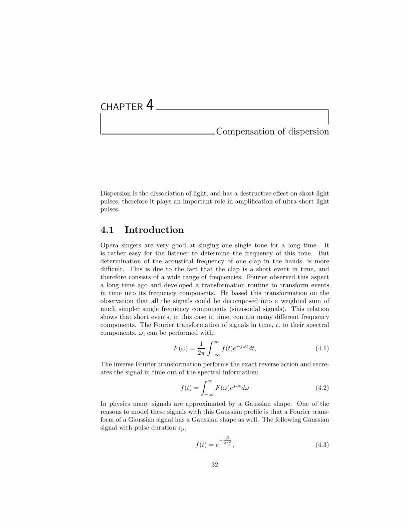
In physics many signals are approximated by a Gaussian shape. One of thereasons to model these signals with this Gaussian profile is that a Fourier trans-form of a Gaussian signal has a Gaussian shape as well. The following Gaussiansignal with pulse duration τp;

f(t) = e−

t2

2τ2p , (4.3)

32

can be Fourier transformed according equation (4.1) to:

F (ω) =τp√2π

e−ω2τ2

p

2 (4.4)

Which is also a Gaussian profile, but its spectral width scales with the inverse ofthe time duration τp, as expected. The relation between the spectral FWHM1

(4ω) and the FWHM of the time duration (4t) can easily be calculated asfollows:

e−

( 124t)2

τ2p =

1

2⇒ 4t = 2τp

√ln2 (4.5)

e−( 124ω)2τ2

p =1

2⇒ 4ω = 2

√ln2

τp(4.6)

Multiplication of these half widths gives the relation between the spectral widthand the time duration of Gaussian shaped signals.

4ω · 4t = 4ln2 (4.7)

This relation alone is not enough to describe a short pulse, although a tungstenlight bulb has a very broad bandwidth, it does not produce short pulses. Inorder to produce short pulses the different colours from the light must arriveat the same time and place. Since we are speaking about waves in this case itis more easy to state that all the different waves, having different wavelengths,should all have one of their maxima coincide with each other to have full positiveinterference at that particular time and place. This is also visualised in figure4.1. As this positive interference occurs at the scale of wavelengths this isalso called the spectral phase relation of the light waves. As lamb bulbs emitno coherent light, creation of this phase relation is impossible. Lasers on thecontrary can produce coherent light. The disadvantage of a simple laser isits narrow the spectral bandwidth. Mode locked lasers have been developedto overcome these problems. They combine a broad spectral width with thecoherency of laser light. In this manner these lasers can produce ultra shortlaser pulses with a well defined spectral phase relation. Figure 4.1 shows thedifference between random added colours, and a sum of colours with a phaserelation. Once an ultra short pulse has been created, it is of vital importanceto conserve the spectral phase relation. The pulse length will be affected bydisturbances in the spectral phase. When light travels through a dispersivemedium like glass the red spectral component will travel faster than the bluespectral components, in this manner the pulse will be stretched, as the spectralcomponents arrive at different times at the detector, as shown in figure 4.2.This separation of spectral components in time is called chirp2. Linear spectralphase disturbance does not affect the pulse shape, it only introduces a delayin travel time through the medium. The following images show sinusoids withdifferent frequencies and the sum of these sinusoids compose a pulse in time asin figure 4.3. In the second image a linear spectral phase has been introducedand the sum of signals show that the pulse energy has been shifted to the side,which means that an extra time delay has been generated. Unfortunately most

1Full Width Half Maximum2The name ”chirp” origins from the sound of a bird, as most birds sing a scale of tones in

one call. Starting with low tones and scaling up to higher ones.

33

Random spectral phase

-1

0

1

2

3

4

5

6

7

8

9

10

-7 0 7Time (au.)

Mode

am

plit

ude

-8

-3

2

7

12

17

22

Inte

nsity:

(su

mo

fa

llm

od

i)^2

Locked frequency modi

-1

0

1

2

3

4

5

6

7

8

9

10

-7 0 7Time (au.)

Mo

de

am

plit

ud

e

-10

-5

0

5

10

15

20

25

30

35

40

Inte

nsity:(s

um

ofa

llm

od

i)^2

Figure 4.1: Sum of locked and random spectral phases

Time

Lig

ht e

lec

tric

fie

ld

Figure 4.2: Impression of chirped pulse

materials introduce a rather complex spectral phase disturbance (φmat(λ)), dueto their wavelength (λ) dependent refracted index (n(λ)). This spectral phasedisturbance scales linear with the length of the material (lmat).

φmat(λ) =2πn(λ)lmat

λ(4.8)

Since the linear spectral phase disturbance has no influence on the pulse durationit is interesting to determine the types of spectral phase disturbances that dodestructively affect the pulse shape. Therefore it is convenient to start with aninput pulse in the time domain, and analyse the deformation of the pulse after ithas passed through a dispersive system, as described in [3]. An arbitrary inputpulse in the time domain can be written as:

E(t) = ξ(t)ei[ω0t+σ(t)]. (4.9)

Here the slowly varying envelope is ξ(t) and the central carrier frequency isω0, while the σ(t) is the temporal phase. In case of a Gaussian pulse where

ξ(t) = ξ0e−(t2/τ2) and σ(t) = 0, the expression for the input pulse changes to:

E(t) = ξ0e−(t2/τ2)eiω0t (4.10)

The Fourier transform of this Gaussian pulse gives us the corresponding ampli-tude and phase in frequency space,

G(ω) =

∫ ∞

−∞

E(t)e−iωtdt = g(ω)eiη(ω) (4.11)

Where g(ω) and η(ω) are the spectral amplitude and phase, respectively. Thisis a more convenient form for the discussion of the spectral phase disturbances

34

w

w

w

w

w

w

1

2

3

4

5

6

w

w

w

w

w

w

1

2

3

4

5

6

j( )=0 p

j( )=0.2 p

j( )=0.4 p

j( )=0.6 p

j( )=0.8 p

j( )=1 p

Time Time

Figure 4.3: Visuatisation of pulse delay due to linear spectral shift

introduced by materials. The output in the spectral domain of the system isthen simply:

G′(ω) = G(ω)S(ω) = g(ω)s(ω)ei[η(ω)+φ(ω)]. (4.12)

Here the complex transfer function S(ω) includes the spectral transfer function(s(ω)) and the spectral phase contribution (φ(ω)) of the system. At this pointthe spectral phase contribution (φ(ω)) is of main interest, since this term has alarge influence on the pulse shape at the output of the system in the time domain.The spectral transfer function (s(ω)), describes the spectral amplification orattenuation of the system. The s(ω) term does not affect the spectral phaserelation. For this reason this term has not taken into account during the designof a dispersion free system. It does affect the bandwidth of the system, asdiscussed in section 3.1. The pulse shape in the time domain E′(t) after passingthrough the system can then be derived by applying inverse Fourier transform:

E′(t) =1

2π

∫ ∞

−∞

G′(ω)eiωtdω (4.13)

Note that when a dispersive free system has been created, the output pulse hasthe same shape as the input pulse.Now the main target is to determine the φ(ω) of the optical system. This spec-tral phase disturbance depends on the refracted indices of the materials used.Those material properties are all functions of the wavelength, and are rathercomplex. Taylor expansion can be applied to the spectral phase. This affectsthe accuracy of the calculations, but minimises the complexity to an acceptablelevel. Attempts to avoid this simplification step resulted in expressions, thatwere too complex to solve manually or with the help of programs like Maple.Fortunately the accuracy of the Taylor approximation is sufficient to optimisethe set-up for a minimum of dispersion. The following expression shows theTaylor series of the spectral phase:

φ(ω) = φ(ω0)+φ′(ω0)(ω−ω0)+1

2φ′′(ω0)(ω−ω0)

2+1

6φ′′′(ω0)(ω−ω0)

3+... (4.14)

The main interest here is to analyse the deformation of the light pulse in thetime domain. The main disturbance here is that some spectral componentstravel faster through a medium and stretch the pulse length. Therefore weare mainly interested in the transit time of the spectral components through amedium. The change of the phase introduced by material is given by

φ(ω) =Lmatn(ω)

c· ω, (4.15)

35

where the travel time through the medium is T (ω) = Lmatn(ω)c . Then the transit

time through a dispersive medium becomes:

T (ω) =δφ(ω)

δω(4.16)

The transit time of a quasi monochromatic wave is then:

T (ω) =δφ(ω)

δω= φ′(ω0) + φ′′(ω0)(ω − ω0) +

1

2φ′′′(ω0)(ω − ω0)

2 + ... (4.17)

Here the derivatives of the spectral phase with respect to frequency: φ′, φ′′ andφ′′′ are respectively known as the group delay dispersion (GDD), group velocitydispersion (GVD), third order dispersion (TOD), etc. Just like the figure 4.3predicts, the linear element of the spectral phase (GDD) only introduces adelay in transit time, but the higher order components introduce independenttransit times for the different spectral components around the central frequency,and smear out the power of the pulse in the time domain. An impressionof a chirped pulse due to GVD shown in figure 4.2 [3]. When a Gaussianshaped pulse contains no GVD and higher order dispersion, the pulse is calledFourier transform limited, as the inverse Fourier transform of this Gaussianpulse produces the same pulse shape as the input pulse.

4.2 Dispersion compensation

In order to create high power ultra short pulses it is of vital importance thatthe system does not introduce second- and higher order dispersion as shownin the previous paragraph. The used pulse amplification system, called chirpedpulse amplification (CPA), is based however on introducing chirp in a controlledmanner. Therefore modelling of the dispersion is an important issue. Modellingof the set-up was mainly performed in programmes like the Disperse-O-Magic(DOM) [18] and by a numerical model in Mathcad [20]. During the construc-tion period of the regenerative amplifier, the design was altered and a reviewof the model had to be performed. The laser system consists of a stretcher,amplifier and compressor. Because different gratings are used in the designs ofthe stretcher and the compressor they don‘t fully compensate for each other.In this manner higher order dispersion, introduced by the materials used in theset up, can be compensated [13]. The easiest way for fine tuning the dispersionof the system to a minimum, can be performed by changing the parametersof the compressor. The mathematical models used showed some ambiguous re-sults. DOM for example shows an optimisation number, but this number is onlybased on the GVD. This means that it is possible to compensate a false prop-erty by another, creating more than one unique solution. With Mathcad thecirculation of many versions caused some misunderstandings, apparently minordifferences in the program creates large differences in the result. Two of thesesolutions have been built without satisfactory results. Another program basedon an analytical model of the dispersion behaviour of the system has been writ-ten in Maple. This to fully comprehend the physics and to find an unambiguoussolution to this problem.The philosophy behind the choice of using Maple to create a new model, isthe fact that all the current models are based on numerical calculations. Maple

36

performs the calculations in an analytical manner, this is only possible when themodels of the dispersive element are also represented in an analytical manner.For this reason a analytical model is used to describe the spectral phase of thestretcher and compressor. The Sellmeier equations can also be differentiated inan analytical manner. This analytical approach makes it possible to plot severalparameters with arbitrary chosen input parameter, without recalculation of thewhole model. This option makes it easy to plot a dispersion landscape for thedispersion terms as function of the settings of the compressor like its gratingangle and grating separation distance. The visualisation of the dispersion wouldcreate much more feeling for the behaviour of the experimental set-up.In order to design the compressor to compensate the system dispersion threesteps have to be taken into account to produce a model and to calculate theoptimal settings of the system.

• Inventory of the dispersive elements in the set up

• Putting the gathered data in one mathematical model

• Find the optimal settings

4.2.1 Inventory of the dispersive elements in the set up

To make an inventory of the dispersive materials, all of the material lengthsas well as its type had to be determined. Many materials were well defined,some had to be measured and in a single case it had to be estimated. Table4.1 presents the material lengths in centimetres of our set-up. The names used

Length in cm of dispersive materials used in the experimental set-upElement o-DKDP BK7 TGG e-Calcite o-TiSaIn the oscillator

TiSa crystal (TS1) 0.5Cavity mirror (M6) 0.95Outside the regen

Beam splitter (PBS1) 0.7728Faraday rotator 2x (FR2) 4Faraday isolator (FR1) 2 3.332Beam sampler (BS3) 0.566Beam expander 0.63In the regen per round trip

Pockels cell (PC) 4 2Beam splitter (PBS2) 1.6345TiSa crystal (TS2) 5.08

Table 4.1: Length of dispersive materials used in the experimental set-up

correspond to the labels used in the design of the complete set-up as shownin appendix A, this table does not take the multi pass amplifier into account.The beam expander has not been included in this drawing of the design, butis has been used in the experiment. The oscillator creates a non dispersedpulse, due to its inner dispersion compensation performed by a prism pair. The

37

only dispersion induced in the oscillator originates from the last pass throughthe resonator cavity, and the elements responsible for the non-compensateddispersion are the TiSa crystal and the out couple mirror. A significant part ofthe material dispersion is generated by the regenerative amplifier as the lighttravels approximately 15 times up and down the regenerative amplifier andthus passing through these materials 30 times. To calculate the dispersionintroduced by these materials, the corresponding Sellmeier equation has to befound, for which several sources are used. The main part of this information isfound in [19] and others on the internet at the site of the manufacturer. TheSellmeier equations used, can be found in the Maple routine on the appendedCD B. The Sellmeier equations represent the refractive index as a function ofwavelength n(λ), and therefore have to be rewritten to calculate the spectralphase disturbances by:

2πlmatn(λ)

λ= φ(λ) (4.18)

And

λ =2πc

ω(4.19)

Using these equations the Sellmeier equations can be rewritten to spectral phasedisturbance as function of material length lmat, and frequency ω.For calculation of the phase disturbance introduced by the compressor, φ(ω)should be determined. Starting with determination of the path length throughthe compressor: The path length ~P is the sum of the two distances ~ab and ~bc,

Output

InputGrating

GratingRetro

reflector

Lgq

b

a

c

Figure 4.4: Schematic of compressor

~ab =Lg

cos(θ), (4.20)

and~bc = ~ab · cos(γ − θ), (4.21)

merging these two together according

~P = ~ab + ~bc =Lg

cos(θ)· (1 + cos(γ − θ)) (4.22)

38

Now the angles do depend on each other and on the wavelength, according tothe grating equation for the first order diffraction:

sin(γ) + sin(θ) =λ

d(4.23)

where d is the groove spacing. The group delay is given by τ = P/c. Since thediffracted angle is larger for longer wavelengths, a transform-limited pulse willemerge negatively chirped (short wavelengths precede longer wavelengths). Thephase of the grating compressor can be derived in a number of ways owing tothe arbitrary choice of an absolute phase and group delay (transit time). Themost compact expression is given by Martinez et al.[16] originating from theequivalent optical path length:

P =φc

ω= Lgcos(θ) (4.24)

Solving this expression for φ using the grating equation 4.23 gives the phase ofa single pass through the compressor:

φ(ω) =ωLg

c

√

1 − (2πc

ωd− sin(γ))2 (4.25)

The design of the stretcher contains an extra telescope between the gratings.This telescope makes a projection of the first grating behind the second grating.As all the path lengths to this imaginary projection of the first grating areaccording the definition of an image of equal length. The distance between thisimaginary grating and the second grating is then the same grating distance asis used for the compressor. Therefore the same equations hold for the stretcheras for the compressor, only the separation distance of the gratings is of oppositesign, and has to be taken from the projection of the first grating to the secondgrating as shown in figure 2.8.

4.2.2 Creation of the Maple model with the gathered data

Once all the Sellmeier equations of the materials and the corresponding materiallengths are gathered, the spectral phase disturbance introduced by the materialcan be derived according to equation 4.15. For calculation of the spectral phasedisturbance of the stretcher and compressor, equation 4.25 is used. The sum ofthese equations form an expression for the spectral phase of the entire set up.According to equation 4.17 the GVD, TOD, FOD and higher order dispersioncan be determined by differentiation to the appropriate level. Note that theunits of the GVD, TOD, FOD, etc. are normally expressed in respectivelyfs2, fs3, fs4, etc. As the whole model derives these spectral phases in seconds,a conversion factor of respectively 1030, 1045, 1060, etc. have to be applied.The model in Maple describes the dispersions as functions of the adjustableparameters. In that manner graphs of the dispersion can be plotted as functionof grating distance (Lg), grating angle (γ) or any other important parameter ofinterest. See the appended CD B for the routine.

4.2.3 Find the optimal settings

The trigger to make another mathematical model of the system, were the poorresults of the first two designs based on the available models. The whole set-up

39

had been built already, and only the compressor had to be set to an optimalconfiguration to cancel the dispersion. The only tunable parameters are thegrating distance (Lg) and the grating angle (γ) of the compressor, thereforethe first plots concern the dispersion of the whole set up as function of theseparameters. Off course it is possible to produce other plots of the dispersion asfunction of other parameters like grating periodicity of the stretcher grating, butas these options are not available the number of free adjustable parameters arelimited to the grating distance (Lg) and the grating angle (γ) of the compressor.The ”dispersion landscape” provides much feeling about the response of thesystem on these settings, and makes it more easy to find the optimum in the lab.The ”dispersion landscape” also showes the optimal settings for the compressor,and these settings appeared to be very accurate. The image of the ”dispersionlandscape” is shown in figure 4.5. It shows the three most important dispersioncomponents GVD, TOD and FOD. A zero pane has been plotted as reference.

FOD

ZeroGVD

TOD

FOD

ZeroGVD

TOD

Figure 4.5: Dispersion landscape, the three orders of dispersion as function ofLg and γ

The ”dispersion landscape” directly shows that it is not possible to cancel out allof the three dispersion components at the same settings. The optimal situationthat can be realised is to cancel out only the GVD together with the TOD.To calculate this point, the two intersection lines of the GVD with the zeropane and the TOD with the zero pane, the crosspoint of these lines is thanthe optimal setting of the compressor. At this point the GVD as well as theTOD is then zero. The Maple routine also determines this point automatically.Another knob on the set-up is the knob to adjust the amount of round trips ofthe pulse through the regenerative amplifier. Although adjustment of the roundtrips through the regenerative amplifier affect the amplification efficiency, it isinteresting to see what happens with the dispersion of the set-up when morematerial is introduced by more round trips through the regenerative amplifier.In first approximation, the regen round trips were set to 16 cycles, re-plotting thedispersion landscape for different values of regen round trips shows the followingdevelopments on the dispersion landscape. Note that the orientation of the plothas changed to a view from above. In this manner it is clearly visible at whichpoints the dispersive components are equal to zero, as the intersection of thedispersion components with the hatched zero plane form a line. The hatched

40

triangle is the visible zero plane where all the dispersion components are smallerthan zero. On the corners of this triangle two of the dispersion components areboth equal to zero. Now the goal is to have all these corners merged intoone point, making all the three dispersion components equal to zero, for onesingle compressor setting. By looking at the figure 4.6 it becomes clear that

0.9 0.92 0.94 0.96 0.98 1 0.9 0.92 0.94 0.96 0.98 1

L_comp (m)

0.9 0.92 0.94 0.96 0.98 1

70

72

74

76

78

80

Alp

ha

(d

eg

)

16 roundtrips 20 roundtrips 23 roundtrips

Figure 4.6: Changes observed in the ’dispersion’ landscape due to additionalround trips in the regen

introducing more material dispersion [21] by increasing the regen round trips,the amount of residual FOD develops to a minimum. The optimal number ofcycles through the regenerative amplifier can be found by plotting the residualFOD as a function of regen round trips. As shown in figure 4.7, the GVD andthe TOD are optimised to zero by adjustment of the set-up parameter to eachof the derived points.

FOD as function of regen roundtrips

-100

-50

0

50

100

22 23 24 25 26

Number of roundtrips

FO

D(1

0^3

fs^4

)

Figure 4.7: FOD as function of regen roundtrips

The optimal situation in the model predicts an optimal dispersion compen-sation for the present situation when the compressor parameters are set toγ = 74.10 deg and Lg = 96.5cm, with 24 cycles through the regenerative ampli-fier. An alternative method of compensation of higher order dispersion can beperformed by adding extra material like BK7-glass or other materials. The fol-lowing table shows the required amount of a single piece of additional materialto compensate the FOD of the set-up. These numbers are based on 16 roundtrips in the regenerative amplifier while the optimal settings of the compressorwere recalculated.Although minor adjustments to the compressor settings have to be made to

41

Options for compensation of FOD by additional materialMaterial additional length (cm)BK7 108.7Sapphire 83.3TGG 29.7Calcite 140DKDP 114

Table 4.2: Dispersive elements

compensate for FOD by additional materials, the amount of additional materialis too large to implement it easily. The best option is an additional piece of 29.7centimetres TGG to compensate FOD. It might be possible to insert a piece ofadditional material in the cavity of the regenerative amplifier, in which case only132nd of the material length would be sufficient. For implementation of such apiece of material in the regen cavity, it has to have an anti-reflection coating, orbe placed at the Brewster angle but this last option will introduce large changesin the beam path. An advantage of placement of a second Brewster windowin the could be the compensation of astigmatism in the cavity as measured insection 3.2.4. Some literature, like [11], describes correction of astigmatism bya Brewster window. But this has not been enquired to the full extend in thisthesis.

42

CHAPTER 5

Comparison of mathematical models and experiments

concerning dispersion

In this section the used mathematical models are compared with each otherand with the experimental results. To compensate for the dispersion only twoparameters, the grating angle (γ) and the grating distance (Lg), are adjustablefor optimisation of the GVD and TOD. Compensation of FOD is only possibleby insertion of additional materials. Adjustment of other parameters to tune thedispersion of the experiment is not easily performed as these parameters concernthe properties of the materials used. Adjustments on the grating periodicity, forexample, implicitly means replacement of these expensive devices. The resultsof the following items are discussed:

• Mathcad

• DOM (Disperse O Matic)

• Lab2

• Maple (Developed during this thesis)

• Experimental results

5.1 Comparison of the models in the most idealsituation

The optimal parameters for the set-up were found by the model in Maple, asthe output of this model was the first one that worked well in the experimentalset up. The parameters obtained from the Maple model are used in all theother mathematical models, in order to make a good comparison between theoutputs of the different models. The parameters used are the material lengthsand they are based on the optimal round trips through the regenerative am-plifier for compensation of FOD as visualised in figure 4.7. This figure showsan optimal compensation of FOD for 24 round trips through the regenerative

43

amplifier. The input parameters of the mathematical models are presented intables 5.1 and 5.2, presenting respectively the material lengths and the com-pressor settings.The optimal compressor setting for this configuration derived with the model

Length of materials at 24 round tripsMaterial length (cm)e-calcite 3.33O-DKDP 96BK7 90.135o-sapphire 122.42TGG 6

Table 5.1: Material lengths at 24 round trips

Stretcher settingsIncident angle α 38◦

perpendicular grating distance (Lg) 65.719 cmGrating constant 1200 lines/mm

Table 5.2: Settings of stretcher

in Maple is displayed in table 5.3. Here the grating constant is an input param-eter, as it is not easily adjustable. Comparison of the models used is performedby comparison of the residual GVD, TOD and FOD. In some of the used modelsthe compressor settings are generated automatically, and therefore also takeninto comparison. The next table shows these results of the used models. Thistable shows that the model in Maple and in Mathcad agree well, the compressorsettings agree nicely and the GVD and TOD are in both cases zero. Only theFOD has the opposite sign. The output of the two remaining models presentthe same compressor settings, DOM is forced to these settings, and returns ac-ceptable values for the dispersion (indicating that it is very close to an optimalsetting). Lab 2 also indicates that these settings for the compressor are veryclose to the optimal ones, the indicator used for this result is the generatedSHG-Frog trace in the program.

Note to Maple:As the first good results in practice appeared after applying the configurationderived with the model written in Maple, the output of this model is used tocompare the other models. This does not mean that the output of this model isthe best of all, but since the results in practice were for the first time comparableto the outcome of this model it was more easy to apply these parameters on theother mathematical models to explore the failures made during the use of theother models. The pulse length is not well defined in this model, as only theGVD is used for estimation of the pulse length. Since the GVD is minimised,this value of GVD is only due to rounding errors.

Note to Lab2:In this model the parameter g is not the perpendicular distance of the gratings,

44

Optimal compressor settingsIncident angle (α) 74.12◦

perpendicular grating distance (Lg) 96.53 cmGrating constant 1500 lines/mm

Table 5.3: Optimal compressor settings derived by Maple

Modelled optimal compressor settings at 24 round tripsModel angle Lg GVD TOD FOD τp

(◦) (cm) fs2 fs3 fs4 fsMaple 74.12 96.53 −3.5 · 10−3 1.4 · 10−3 1.04 · 104 25.00Mathcad 73.50 96.06 5.14 · 10−5 1.52 · 10−4 −5.72 · 104 27.46DOM 74.12 96.53 -230.52 -215.62 1.26 · 104 26.65Lab2 74.08 96.52 -70.00 4.00 · 103 5.23 · 103 28.97

Table 5.4: Results of the used models for optimal compressor settings at 24round trips

but the distance between the gratings. When aligned, the angle of the gratingaccording to the optical axis of the stretcher is following the grating equationβ = asin((λ/d) − sin(α)) = 20.14◦ resulting in a grating distance along theoptical axis of 700 mm. As the model for the stretcher defines the distancebetween the grating surface and the focal point as g which is the half of thedistances between the grating and the projection of the second grating. There-fore one has to use g = 350 mm and use two identical stretchers as the set-upconsist of a four pass stretcher, while a stretcher has minimally 2 passes. Also

Figure 5.1: stretcher parameters in Lab2

the outcome of the compressor settings from the model in Lab2 are conformthis approach, and have to be transformed to compare the results with theother mathematical models. Hereby the transmittance angle of the compressorgrating is than βcomp = 13.77◦, and the axial distance between the gratings of

45

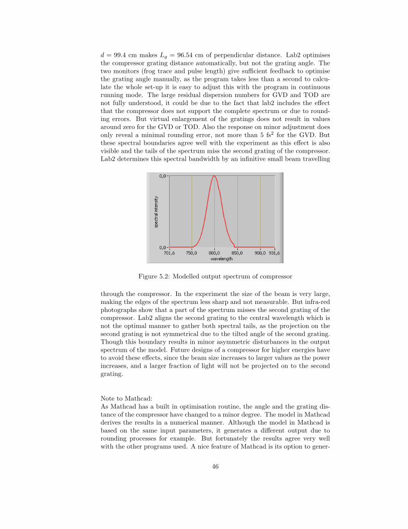
d = 99.4 cm makes Lg = 96.54 cm of perpendicular distance. Lab2 optimisesthe compressor grating distance automatically, but not the grating angle. Thetwo monitors (frog trace and pulse length) give sufficient feedback to optimisethe grating angle manually, as the program takes less than a second to calcu-late the whole set-up it is easy to adjust this with the program in continuousrunning mode. The large residual dispersion numbers for GVD and TOD arenot fully understood, it could be due to the fact that lab2 includes the effectthat the compressor does not support the complete spectrum or due to round-ing errors. But virtual enlargement of the gratings does not result in valuesaround zero for the GVD or TOD. Also the response on minor adjustment doesonly reveal a minimal rounding error, not more than 5 fs2 for the GVD. Butthese spectral boundaries agree well with the experiment as this effect is alsovisible and the tails of the spectrum miss the second grating of the compressor.Lab2 determines this spectral bandwidth by an infinitive small beam travelling

Figure 5.2: Modelled output spectrum of compressor

through the compressor. In the experiment the size of the beam is very large,making the edges of the spectrum less sharp and not measurable. But infra-redphotographs show that a part of the spectrum misses the second grating of thecompressor. Lab2 aligns the second grating to the central wavelength which isnot the optimal manner to gather both spectral tails, as the projection on thesecond grating is not symmetrical due to the tilted angle of the second grating.Though this boundary results in minor asymmetric disturbances in the outputspectrum of the model. Future designs of a compressor for higher energies haveto avoid these effects, since the beam size increases to larger values as the powerincreases, and a larger fraction of light will not be projected on to the secondgrating.

Note to Mathcad:As Mathcad has a built in optimisation routine, the angle and the grating dis-tance of the compressor have changed to a minor degree. The model in Mathcadderives the results in a numerical manner. Although the model in Mathcad isbased on the same input parameters, it generates a different output due torounding processes for example. But fortunately the results agree very wellwith the other programs used. A nice feature of Mathcad is its option to gener-

46

ate a representation of the output pulse, as shown in the figure 5.3. One special

Figure 5.3: Theoretical intensity profile of the pulse

note has to be made concerning the use of the model in Mathcad. The names forthe delay time ”T” and second order dispersion ”GDD” should be named GDD(group delay dispersion) and GVD (group velocity dispersion) respectively. Butas these names are integrated into the whole model, the change of these namesconsumes too much effort for the same result.

Note to DOM:The Disperse-O-Magic is a fast tool to check your system, the disadvantageis that no optimisation routine has been built in. But by moving the slidersgently, some optimal configurations can be derived, taking into account thatthe estimated output pulse length is only derived in the GVD, as the influencesof higher order dispersion is not taken into account. This makes it possible toend up with several optimal configurations, as only one optimal configurationexist. The output here has not been optimised, therefore the GVD, TOD andFOD are again quite large, but still not destructively high. Manual optimisationeasily drives these values to a minimum around zero with only tenths of a degreeadjustments to the compressor grating angle and a few millimetres adjustmentsto the compressor grating distance. The conclusion can be drawn that DOMagrees well with the other models. A comment concerning this program is thatGVD is called GDD, which is an incorrect name for GVD.

5.2 Comparison of the mathematical models tothe experiment

In the experiment it is hard to approximate the theoretical optimum. In thiscase the models are mainly based on the practical experiment, but the roundtrips in the regenerative amplifier were not fixed yet, since at that momentof design of the models no fixed number of round trips had been chosen yet.

47

Now the regenerative amplifier has been optimised, restricting the variation ofnumber of round trips. As this number of round trips does not agree with theoptimal number of 24 round trips, the outcome of the mathematical modelsdiffer from the optimal result. Now the best solution has to be found for theexperimental set-up with only 16 round trips through the regenerative amplifier.In this experimental case it is only possible to compensate the GVD and TOD,which is possible by adjustments of the compressor angle and compressor gratingdistance.

5.3 Determination for regen roundtrips

After fine tuning of the Regenerative amplifier to an optimal output power andstability the number of round trips can not be measured directly with the detec-tor placed at its default position ’B’, as in this manner the moment of injectionis not detectable. For determination of the injection moment moment, the de-tector has to be installed in position ’A’. When the injection and extractionmoments are obtained, it is possible to calculate the time the pulse is capturedin the cavity. With the deterctor in position ’B’, it is possible to measure du-ration time of one cycle. With these numbers it is possible to determine thenumber of roundtrips that the pulse makes through the regenerative amplifier.The images obtained at the scope at the corresponding positions of the detec-tor are shown in figure 5.4. With the detector arranged at position ’A’, the

Figure 5.4: Positions of photo detector and their signals presented at the scope

moment of injection can be fine-tuned easily; as long as the amplitude of thelast ”spike” before the moment of injection is attenuated it is not correctlyinserted into the regenerative amplifier. Measurements showed that it is onlypossible to fine-tune the moment of injection with help of a Grenouille trace ofthe re-compressed output pulse. This Grenouille trace shows the influence of thematerial dispersion when it is injected at a wrong moment. If this Grenouilletrace is not available, then the optimal injection moment has to be determinedwith a detector placed at position ’A’.Optimal settings for the regen showed a pulse capture time of 200 ns. The roundtrip time for this cavity of approximately 1.8 meters length should be around 12ns, measurements showed that 7 round trips take 87 ns, which corresponds to around trip time of 12.43 ns. Dividing the capture time through this measuredround trip time gives 16 round trips through the regenerative amplifier. As theregenerative amplifier has been optimised for a stable output this number ofround trips is used to determine the optimal settings for the compressor.

48

5.4 Modelling of the set-up according to the ex-

perimental settings

In order to make a nice comparison with the ideal case all of the available modelsare again used and compared with each other and the experiment.

Length of materials at 16 round tripsMaterial length (cm)e-calcite 3.33O-DKDP 64.00BK7 61.063o-sapphire 81.78TGG 6.00

Table 5.5: Material lengths of the experimental set up

Compressor settings based on 16 round tripsModel angle Lg τp

(◦) (cm) fsMaple 71.24 94.39 25.00Mathcad 71.12 94.33 37.98DOM 71.24 94.38 25.01Lab2 71.26 94.39 29.32Experiment 74.6 ±0.5 94.6 ±0.5 29 ±1

Table 5.6: Comparison the outcome of the mathematical models with the ex-perimental results.

Note to Lab2:The outcome of the Lab2 model has to be transformed to compare the resultswith the other mathematical models. Hereby the transmittance angle of thecompressor grating is then βcomp = 14.66◦, and the axial distance between thegratings of d = 97.56 cm makes Lg = 94.39 cm of perpendicular distance. Op-timisation is again performed by manual adjustments of the grating angle, asthe grating distance is automatically optimised, providing fast reliable results.An interesting feature of this package is the option to plot a SHG FROG trace.As the trace of a SHG FROG is identical to a Grenouille trace, which is themeasurement method used in the experimental set-up. Therefore it is a nice toolto analyse the output in case it is not fully compensated. Images of these tracesare used to compare the output of the set-up with the mathematical models 5.5.

Note to DOM:The grating distance has been chosen to be the same as the Maple output, andsmall adjustments to the grating angle results in a low value for the GVD, andas the pulse duration is based on that figure, it is almost equal to the the inputpulse duration of 25 fs.

49

5.5 Conclusions concerning the comparison be-

tween the mathematical models and the ex-perimental results

The pulse duration shows large differences among the different models, the es-timated pulse duration by Maple and DOM are only based on the GVD-termof the dispersion. As this value is controlled to an optimal value of zero, thepulse would have the same duration as the input pulse. Mathcad derives thepulse duration by taking the FWHM of a reconstructed envelope of the pulsethat is based on the GVD, TOD, FOD and FifthOD. This sophisticated methodgenerates, in contrast with the expectations, a pessimistic result of almost 38fs. pulse duration. The reason for this difference can not be discovered, as allthe equations used in the Mathcad routine agree the theory. Though this largervalue of the pulse length is mainly induced by the FOD and the FifthOD. Theresults of Lab2 show the best agreement with the experimental values, concern-ing the pulse duration, the disadvantage is that it is not fully transparent howthese numbers are generated. A nice option in Lab2 is to generate a Frog trace,this image can be compared with the trace from the experiment by a Grenouille,as the traces generated by a Grenouille or a Frog apparatus provide an identicalinterpretation of the pulse. The images are presented in figure 5.5. The shape of

Measured frog trace Simulated frog trace

Figure 5.5: Measured Grenouille trace and derived Frog trace by Lab2

the images show large agreements, but the scale of the wavelength in the Lab2model is not correct due to unknown reasons. But also the software used tomeasure the Grenouille trace of the experiments shows some errors during cali-bration of the wavelength axis. Therefore the measurements on the bandwidthcould only be made by an external spectrometer. The scale of the measuredwavelength in this graph agrees well with the spectrometer, even though thecalibration was not successful. It can be concluded that the comparison of theexperiment and the Lab2 model show large agreements, therefore Lab2 is a nicetool to predict the behaviour of the set up, including comparison of almost allthe diagnostics that can be performed in the experiment.

The derived settings of the compressor show some differences with the settings

50

obtained in the experiment, especially the grating angle. These differences canlargely be explained by misalignment of the stretcher. Adjustments to the inputparameters of the Maple model, show that a stretcher angle of 39◦ instead of38◦ result in compressor settings of: Lcomp = 0.94 metres and an angle of 73.7◦,whose are much closer to the values of the experiment. This, combined witha small red shift of the spectrum to 810nm, let the model in Maple come to aresult of Lcomp = 0.94 metres and an angle of 74.03◦.

As the mathematical models derive the settings for the compressor very well,it is also interesting to explore the case when some parameters are changedto the set-up, and have the compressor settings be adjusted to re-compensatefor the dispersion. This can be easily tested by adjustment of the numberof round trips that the pulse is travelling through the regenerative amplifier.During this test the number of round trips through the regenerative amplifier areadjusted, and only the grating distance of the compressor is modified to optimisethe output pulse length. A Grenouille is used to check the output pulse. Tomeasure the small differences of grating distance a micrometer is used to measurethe displacement of the second grating. To determine the absolute gratingdistance, the average distance differences between the measured points and thepoints derived by the Maple model have been added to the measured points,for easier to comparison of the mathematical model to the experiment. Othermeasurements show that this absolute grating distance is in the experimentslightly different from the distance derived by the model in Maple, which hasbeen explained by minor alignment errors in the compressor. As the micrometermeasures the translated distance along the optical axis, all measured points areconverted to the perpendicular grating distance. In the model in Maple thegrating angle is fixed to the optimal setting corresponding to 16 round trips, andonly the grating distance is used to find the minimal GVD, which is basically thesame action as performed in the experiment. The results are presented in figure5.6. As this graph shows good agreements between the model in Maple and the

Grating distance as function of regen roundtrips

970

972

974

976

978

980

982

984

986

12 14 16 18 20 22

Regen roundtrips

Gra

tin

gd

ista

nc

e(m

m)

Simulated

Measured

Figure 5.6: Grating distance as function of round trips in the regen, experimen-tal results compared with the outcome of the mathematical model

experiment, it is a nice basis to predict the settings of the compressor for the two

51

last stages including the 4-pass and 2 pass amplifiers. Since the expectation isthat the additional TiSa crystal introduced to the system will have only minorinfluence on the dispersion, only minor adjustments will presumably have tobe made concerning the compressor settings. Therefore the idea is to calculatethe differences in the compressor settings instead of the absolute settings aspresented in the table 5.7.

Compressor settings for additional multi-pass amplifiersParameter optimal setting 4-pass 4- and 2-pass

for 16 passes abs. 4 abs. 4Angle (◦) 71.24 71.47 0.23 71.57 0.33Lcomp (cm) 94.39 94.58 0.19 94.65 0.26

Table 5.7: Estimated compressor adjustments after installation of multi-passamplifiers

These numbers are based on the parameters for the set-up with 16 passesthrough the regenerative amplifier, the two additional multi-pass amplifiers in-troduce only dispersion due to the TiSa crystal. The first 4-pass amplifierconsist of an 18 mm TiSa crystal, and the last 2-pass amplifier is based on a15 mm long TiSa crystal. This table reveals the expectation that additionaldispersion introduced by the multi-pass amplifiers will have a minor influenceon the compressor settings. But as the power of the pulse increases duringthese amplification stages, the beam size must increase as well to avoid damageto the optics. The increased beam size requires a larger second grating of thecompressor, as it is already a bit too small for this purpose, displayed in figure5.2 which is generated by the model of Lab2.

52

CHAPTER 6

Measurement of the output pulse

A Grenouille has been used to measure the final output of the experiment. Inorder to perform a good measurement on the pulse, the Grenouille has to becalibrated first. This section will discuss how the grenouille has been calibratedas described in [14], and finally the measured pulse shape of the output of theexperiment is presented.

6.1 Calibration of the Grenouille

To calibrate the Grenouille a well defined pulse is used from the oscillator. Theoutput of the oscillator is not completely dispersion free due to the last non-compensated pass through the crystal and the out-couple mirror of the oscillatoritself. This compensation of dispersion is performed by prism compensation [22].A thin film beam splitter and two mirrors are used to create a double pulse ofthis dispersion free pulse. Now this double pulse is put into the Grenouillefor the actual calibration. Note that all the wavelengths must be halved, as a

OscillatorPrism compressor

Creation of

double pulse

Grenouille

Setup for calibration of the grenouille

Figure 6.1: Setup for calibration of the Grenouille

frequency doubling crystal is used.Two calibration measurements have been performed, and their Grenouille tracesare shown in figure 6.2. The corresponding spectra, measured with an Ocean

53

Measurement 1 Measurement 2

Figure 6.2: Grenouille traces of double pulse for calibration

optics USB2000 spectrometer, are presented in figure 6.3.

Spectrum corresponding to calibration measurement 1

0,0

0,2

0,4

0,6

0,8

1,0

760 770 780 790 800 810 820 830

Wavelength (nm)

Inte

ns

ity

(a.u

.)

Spectrum corresponding to calibration measurement 2

0,0

0,2

0,4

0,6

0,8

1,0

760 770 780 790 800 810 820 830

Wavelength (nm)

Inte

ns

ity

(a.u

.)

Figure 6.3: Measures spectra of double pulse, for calibration

Plotting the positions of the spectral peaks onto their pixel positions in theGrenouille trace in one graph, shown in figure 6.4, will produce a straightline. The slope of this line represents the value of the calibration parameterSλ (nm/pixel) for the spectral axis of the program.Along the time axis of the Grenouille trace, as shown in figure 6.2, three lobesare detected. The autocorrelation signal of two pulses generate a signal withthree maxima. The first maxima, due to overlap of the first pulse with thesecond pulse, and in the central maxima is caused as both pulses overlap witheach other (stronger signal), and the last maxima in the autocorrelator signalrepresents the overlap of the last with the first pulse, shown in figure 6.5.For calibration of the time axis the separation time τsep must be determined,this can be derived from the average separation distance between the spectrallobes 4λ, according:

τsep =λ2

0

4λ · c , (6.1)

where λ0 is the centre wavelength and c the velocity of light. The used 4λin this experiment is the average separation distance between the maxima inthe spectrum. For very broadband pulses, this is not the exact solution; theseparation is constant for frequency, not wavelength. When the bandwidth issmall, this effect is not significant. In the experiment this non-linearity has not

54

Spectral maxima versus pixel position, measurement 1

y = 0,0418x + 387,45

388

392

396

400

404

408

0 100 200 300 400 500

Position in Grenouille trace (pixel)

Co

rre

sp

on

din

gw

av

ele

ng

th,

lam

bd

a/2

(nm

)

Spectral maxima versus pixel position, measurement 2

y = 0,0422x + 387,93

388

392

396

400

404

408

0 100 200 300 400 500

Position in Grenouille trace (pixel)

Co

rre

sp

on

din

gw

av

ele

ng

th

lam

bd

a/2

(nm

)

Figure 6.4: Wavelength of the spectral lobes mapped onto their position in theGrenouille trace

tt

0

0 0

AutocorrelateSignal

Figure 6.5: Representation of autocorrelaat of doublepulse

been observed, therefore this simplified method is used for calibration of thefrequency axis. Once τsep is derived only the average separation distance of thethree lobes in the time direction of the Grenouille trace 4Sτ (pixels) has to bemeasured, to determine the calibration value of the time axis St according:

St =τsep

4Sτ, (6.2)

The measured values for determination of the calibration and the derived cali-bration settings by this measurement are presented in table 6.1. The calibration

Measured values for determination of the calibrationCalibration measurement 1 2 unitAverage 4λ 4.67 3.24 nmτsep 457 658 fsAverage 4Sτ 117 165 pixels

Derived calibration valuesSt 3.905 3.989 fs/pixelSλ (Slope from fig. 6.4) 0.0418 0.0422 nm/pixel

Table 6.1: Measured and derived values for determination of the calibrationvalues

values presented in table 6.1 for the time and wavelength axis, St and Sλ respec-tively, show only a few percent difference between outcome of the two calibration

55

measurements. This indicates that the calibration has been successful and theobtained values for the calibration are St=3.95±0.04 and Sλ=0.042±0.002.

6.2 Measured output pulse

Now the software of the Grenouille has been calibrated, it automatically de-termines the pulse duration. This measurement is performed on the outputof the experiment. The pulse energy, obtained in earlier measurements beforere-compression was approximately 3.5 mJ, and during that same measurementa energy of the pulse after re-compression of 2.5 mJ has been measured, thismeans that a compression efficiency of 71% has been reached. More detailedmeasurements of the grating efficiency can be found in the damage reports atthe appended CD, appendix B. The repetition rate of the laser is 10 Hz, andaccording to the Grenouille trace, the pulse has a duration of 29.6 fs, as shownin the figure 6.6.

Figure 6.6: Output of experimental set up measured with Grenouille

56

CHAPTER 7

Conclusions

This report describes the design and construction of a regenerative amplifierand a grating compressor of a chirped pulse amplification laser as well as thecharacterisation of the output pulse. Also a mathematical model for the analysisof the dispersion of the set-up has been developed. The laser set-up generatesa pulse of 29 fs with an energy of 2.5 mJ, which agrees with the expectations ofthe system.

7.1 Regenerative amplifier

The measured output pulse energy of 3.5 mJ of the regenerative amplifier agreeswell with the expectations, based on theory. The experimental development ofthe beam waist has been compared with a theoretical model and agrees withinthe error margins, taking into account additional effects like thermal lensing.

7.2 Mathematical model for dispersion

Several models have been used and compared to calculate the dispersion in thesystem in order to re-compress the amplified stretched pulse coming out of theregenerative amplifier. The mathematical model in Mathcad has been improvedby addition and correction of the Sellmeier equations used in this model. An-other mathematical model has been written in Maple, and shows accurate valuescompared with the experimental settings. The option for producing a disper-sion landscape provides the experimentalist a good picture of the dispersivebehaviour of the experiment. Now the set-up can be modelled easily, providinginformation concerning adjustments to the settings of the compressor in orderto adapt to changes in the experiment.

7.3 Re-compression of the pulse

The pulse has been re-compressed successfully, with help of the derived design bythe mathematical models. The pulse has been re-compressed with an efficiency

57

of 71%. The spectrum of the pulse has been limited due to the finit dimensionsof the second grating. The final output of the experiment is a 2.5 mJ pulse of29 fs duration, starting from a 25 fs, 3nJ pulse from the oscillator. Thus theregenerative amplifier and the compressor have been successfully constructedand form a good basis for the further development of the 30 TW laser.

58

CHAPTER 8

Recommendations

Working with such a large laser system, reveals many points of attention. Aslong as the system runs every week, only the minor adjustments to the set uphave to performed, this increases the reliability. The overall pointing stabilitycan be improved by covering the whole set-up by boxes to avoid airflow. Thisalso minimises the chance of damage to the optics due to dust particles. Andby putting the laser into a box, the safety increases.

8.1 Regenerative amplifier

The output power of the regenerative amplifier is relatively stable due to thestabilisation effects of the regenerative amplifier, though fluctuations in theefficiency of the amplification can be observed by the manner how the energy ofthe pulse builds up in the cavity. These fluctuation can be caused by fluctuationsof the pump laser. Mode-hopping of the pump laser could cause these effects,asa multi-mode pump laser is used instead of a single-mode pump laser. It is alsopossible that instabilities in the shot to shot power of this pump laser, generatedby its power supply or degeneration of its flash-tubes, causes this effect. For abetter understanding of these minor problems, this effect has to be examinedto a further extend.

Long term measurements on the output power of the regenerative amplifierrevealed a small increase in shot to shot power fluctuations. This could bereadjusted easily, but the exact reason for this effect has not been found yet.For solving these problems it is recommended to monitor the output power ofthe pump laser over a long term. It could also be solved by adjustment of thecooling temperature of the TiSa crystal of the regenerative amplifier.

It has been demonstrated that the spectral behaviour of the regenerative am-plifier can be manipulated by an etalon, manipulation of the spectrum has tobe made in order to retrieve an as broad as possible spectrum around 800 nm,for creation of shorter pulses. A detailed investigation of the etalons influenceshould be performed in future.

59

8.2 Mathematical model for dispersion

The mathematical model of the dispersion of the set-up, does not include errorson the used input parameters. An additional feature would be to calculate mar-gins on the generated compressor settings due to misalignment of the stretcher,as calculations have shown that this could be the cause of minor differencesbetween the model and the experimental settings, shown in section 5.5.

8.3 Re-compression of the pulse

The bandwidth of the compressor is limited due to the size of the second grating,therefore a larger grating has to be installed. As a new grating has to be ordered,it is recommended to re-calculate the compressor settings for different gratingperiodicity of the compressor gratings. At this moment the compressor is set toan angle of 74◦, which is near the limit of the acceptance angle of the grating.The advantage of this large angle, on the contrary, is that the optical power issmeared out over a larger surface of the grating. In this manner a smaller beamsize can be applied without causing damage to the gratings. But, calculationwith 16 round trips and a compressor based on 1400 lines/mm, instead of 1500lines/mm, gratings showed optimal settings at Lg=1.07 meters and grating angleof 58◦, which could have a better grating efficiency, although no significant losseshave been measured on the gratings at the current set-up.

60

BIBLIOGRAPHY

[1] Geng, R.L.; Padamsee, H.; Seaman, A.; Shemelin, V.D., ”World RecordAccelerating Gradient Achieved in a Superconducting Niobium RF Cav-ity”, PAC 2005. Proceedings of the , no.pp. 653 - 655, 16-20 May 2005

[2] R.Bingham, J.T. Medonca and P.K.Shukla. ”Plasma based charged-particleaccelerators.” plasmaphysics and controlled fusion, 46 (2004) R1-R23.

[3] S. Backus et al., ”High power ultrafast lasers”, Rev. Sci. Instrum., Vol 69,No 3, March 1998, .

[4] Arsen G. Khachatryan, ”Trapping, compression, and acceleration of anelectron bunch in the nonlinear laser wakefield”, Physical Review E, vol.65, 046504, 11 April 2002, Yerevan Physics Institute

[5] A.G. Khachatryan, F. A. van Goor, and K.-J. Boller, ”Extremely shortrelativistic-electron-bunch generation in the laser wakefield via novel bunchinjection scheme”, Physical review special topics - Accelerators and Beams,Vol. 7, 121301, 6 December 2004, Department of Applied Science, Univer-sity of Twente.

[6] M.J. van der Wiel et al, ”Laser wakefield acceleration: the injection is-sue. Overview and latest results”, Phil. Trans. R. Soc. A, rsta.2005.1731,Department of applied physics, Center For Plasma Physics and RadiationTechnology, Eindhoven University of Technology.

[7] P. F. Moulton, ”Spectroscopic and laser characteristics of Ti:Al2O3”, J.Opt. Soc. Am. B., Vol. 3, No. 1, January 1986.

[8] C. Barty, T. Guo, C. Le Blanc, F. Raksi, C. Rose-Petruck, J. Squier,A.Tian, K. Wilson, V.Yakovlev, and K. Yamakawa, ”Generation of 18-fs, multiterawatt pulses by regenerative pulse shaping and chirped-pulseamplification”, Opt. Lett. vol. 21, 668 (1996).

[9] G. Cheriaux, et al, ”Aberration-free stretcher design for ultrashort-pulseamplification”, Opt. Lett. 21, 414 (1996)

[10] A. Oeffner, U.S. patent 3,748,015 ( 1971).

61

[11] W. T. Silfast, ”Laser Fundamentals”, 2nd ed. ,Cambridge UK, Cambridgeuniversity press. (2004)

[12] Eugene Hecht, ”Optics”, 4 ed., San Francisco US. Addison Wesley.

[13] J.Squier, C.P.J.Barty, F. Salin, C. Le Blanc, S, Kane, ”Use of MismatchedGrating Pairs in Chirped-pulse Amplification Systems”, Appl. Opt. 37 (9),1638 (1998)

[14] Rick trebino, ”Frequency resolved optical gating: the measurement of ul-trashort laser pulses”, ISBN 1-4020-7066-7.

[15] A.Yariv, ”Quantum electronics”, 3rd. ed. (Wiley, New York, 1989).

[16] Martinez et al, ”Negative group-velocity dispersion using refraction”, J.Opt. Soc. Am. A., Vol. 1, No 10, pag. 1003, October 1984.

[17] P. W. Milonni, J. H. Eberly, ”Lasers”, (Wiley 1988), ISBN 0-471-62731-3.

[18] Prof. C. W. Siders, ”Disperse-O-Matic”, School of Optics / CREOL.

[19] M.Bass, ”Handbook of optics”, Optical society of America (McGraw-HillNew York, 1995).

[20] Dr. Ir. Ing F.A. van Goor. University of Twente.

[21] Florentina Rosca-Pruna, ”Alignment of Diatomic Molecules Induced byIntense Laser Fields”, ISBN 90-9015452-3, 2001, Amsterdam

[22] R. L. Fork, O. E. Martinez, and J. P. Gordon, ”Negative dispersion usingpairs of prisms” Opt. Lett. 9, 150 (1984).

62

APPENDIX A

Schematic of experimental set up

Figure A.1: Scematic of experimental set up

63

APPENDIX B

Additional CD

This CD contains:

• The used mathematical models, Maple, Lab2, Mathcad and DOM

• Calculations concerning the beam waist by matrix calculation

• Damage reports of the gratings

• A copy of this Report

64