Embed Size (px)
Citation preview

c© 2009 International PressAdv. Theor. Math. Phys. 13 (2009) 553–598
D-branes and normal functions
David R. Morrison1,2 and Johannes Walcher3
1Center for Geometry and Theoretical Physics, Duke University, Durham,NC 27708, USA
2Departments of Mathematics and Physics, University of California, SantaBarbara, CA 93106, USA
3School of Natural Sciences, Institute for Advanced Study, Princeton, NJ08540, USA
Abstract
We explain the B-model origin of extended Picard–Fuchs equationssatisfied by the D-brane superpotential on compact Calabi–Yau three-folds. The domainwall tension is identified with a Poincare normal func-tion — a transversal holomorphic section of the Griffiths intermediateJacobian — via the Abel–Jacobi map. Within this formalism, we derivethe extended Picard–Fuchs equation associated with the mirror of thereal quintic.
Contents
1 Introduction 554
2 Normal functions and D-branes 557
2.1 Normal functions attached to algebraic cycles 558
e-print archive: http://lanl.arXiv.org/abs/arXiv/0709.4028

554 DAVID R. MORRISON AND JOHANNES WALCHER
2.2 Abel–Jacobi map on the derived category 561
2.3 Comments on open problems 563
3 The real quintic and its mirror 565
3.1 Six hundred and twenty-five real quintics 565
3.2 The prediction 566
3.3 Matrix factorization 568
3.4 Intersection index 570
3.5 Bundles 572
3.6 From matrix factorization to curve 575
4 Main computation 576
4.1 Sketch of computation 577
4.2 Resolution of singularities 578
4.3 Inhomogeneous Picard–Fuchs viaGriffiths–Dwork 580
4.4 Boundary conditions and monodromy 585
5 Summary and conclusions 586
Acknowledgments 587
Appendix 587
References 594
1 Introduction
Mirror symmetry is a powerful tool to manipulate physical and mathematicaldata associated with Calabi–Yau manifolds. Soon after the earliest exam-ples of mirror symmetry [1–3], a computation of the special geometry andthe enumeration of rational curves on the quintic were made by Candelaset al. [4]. The computation was explained Hodge theoretically in [5] and the

D-BRANES AND NORMAL FUNCTIONS 555
verification of the enumerative predictions was completed in [6,7]. Approachesto derive mirror symmetry from the worldsheet point of view have also beendiscussed [8, 9].
Meanwhile, D-branes have entered mirror symmetry in a variety of ways.To name the most important, Witten [10] showed that for open topologicalstrings, cubic string field theory reduces to ordinary or holomorphic Chern–Simons theory. Kontsevich [11] proposed to understand mirror symmetryas an equivalence of A∞-categories, whose objects were later identified asD-branes. Strominger et al. [12] used D-branes to develop the geometric pic-ture of mirror symmetry as a duality of torus fibrations. Vafa and variouscollaborators (beginning with Gopakumar) have shown that Bogomol’nyi —Prasad–Sommerfield (BPS) states of D-branes are extremely useful invari-ants that carry a lot of physical and enumerative information [13]. Dou-glas [14] has complemented the picture by a general formulation of stabilityconditions on D-brane categories (see also [15]).
In the course of these developments, the established theory underlyingclosed string mirror symmetry for Calabi–Yau manifolds — special geometryand Gromov–Witten invariants — has played a very useful supporting role.It has, however, not always been clear whether D-branes would ultimatelybe part of the traditional picture or how one would derive the closed stringstory, e.g., from D-brane categories. (This problem was posed already in[11]; for some recent work, see [16–18].) As a physicist, one feels that insome sense, the underlying reason is that A∞-categories are too big. SinceD-brane categories are defined off-shell, they carry a lot of redundant, gauge-dependent information. With some hindsight, one is led to ask the naturalquestion: What is the invariant physical information stored in the derivedcategory?
In this paper, we give answers to these questions by picking up the Hodgetheoretic considerations. Our main motivation is the recent realization thatat least in some cases, there is indeed invariant information in the openstring sector beyond its cohomology. Walcher [19] showed that for a certainD-brane configuration on the quintic,1 the on-shell value of the superpo-tential, as a function over closed string moduli space, satisfies a differentialequation which is an extension of the Picard–Fuchs equation which gov-erns closed string mirror symmetry. According to general principles, thissuperpotential makes enumerative predictions in the A-model, which weresubsequently verified rigorously in [22]. In this work, we will explain theB-model origin of this extended Picard–Fuchs equation. Previous studiesof analogous problems in local Calabi–Yau manifolds include [23,24], whose
1Very similar results appear to hold for many other one-parameter models [20,21].

556 DAVID R. MORRISON AND JOHANNES WALCHER
enumerative predictions were verified in [25,26] and whose differential equa-tions were discussed in [27,28] (see also [29,30]).
The main idea to derive Picard–Fuchs equations in the context of openstrings has been implicit in many previous works. Consider, for simplic-ity, the case when we are wrapping a D5-brane on a curve in some secondhomology class of our Calabi–Yau manifold. Assume that this class has twoisolated holomorphic representatives C+ and C−. Choose a three-chain Γ,∂Γ = C+ − C− connecting these two representatives. C+ and C− correspondphysically to two supersymmetric vacua of an N = 1 supersymmetric theoryon the brane worldvolume. The tension of a BPS domainwall between thetwo vacua is, T = W+ − W−, equal to the superpotential difference, and isgiven by the geometric formula [31]
W+(z) − W−(z) = T (z) =∫
ΓΩ(z), (1.1)
where Ω(z) is the holomorphic three-form as a function of complex structuremoduli.
The Picard–Fuchs equation, LΠ(z) = 0, is the (in general, system of par-tial) differential equation satisfied by any period Π(z) =
∫Γc Ω(z) of the
holomorphic three-form over a closed three-cycle, ∂Γc = 0. When apply-ing the Picard–Fuchs operator to a chain integral as in (1.1), we will not,in general, obtain zero. One type of non-vanishing contribution arises as aboundary term, but there are, in general, also other terms from differentiat-ing the chain Γ. The inhomogeneous Picard–Fuchs equation associated withC+ − C− is then
LT (z) = f(z). (1.2)
As we will review below, this inhomogeneous equation is well-defined by thealgebraic cycle C+ − C− and does not depend on the choice of chain Γ. Itis also known (although we will not review this) that f(z) is necessarily arational function of the suitable algebraic coordinate on moduli space.
The general existence of inhomogeneous Picard–Fuchs equations similarto (1.2) has been known in the mathematical literature at least as earlyas [32]. (In dimension 1, of course, such notions are completely classical.)A fairly recent reference with examples worked out in dimension 2 (i.e., forK3 surfaces) is [33]. The main result of the present work is a completeand mathematically rigorous derivation of the inhomogeneous Picard–Fuchsequation satisfied by T (z) for the B-brane mirror to the real quintic. Thisis, to our knowledge, the first explicit example of an inhomogeneous Picard–Fuchs equation in dimension bigger than 2.

D-BRANES AND NORMAL FUNCTIONS 557
The particular form of the inhomogeneous Picard–Fuchs equation for thereal quintic was originally guessed in [19] based on very restrictive mon-odromy properties that its solution should possess. Combined with theresults of [22], our derivation puts open string mirror symmetry for the realquintic at an equal level with the classical mirror theorems on rational curvesin Calabi–Yau three-folds.
Before doing the computation in Section 4 (some details having beendeferred to the appendix), we will describe in Section 2 how normal func-tions and the variation of mixed Hodge structure capture certain invariantinformation of the open string sector. We will not attempt a detailed com-parison with the local toric case [27, 28]. It would be very interesting tounderstand better the relation between those works and ours, especiallywith regard to open string moduli. We also note that the insights into therelation between D-branes and normal functions have proven central in therecent computation of loop amplitudes in the open topological string usingthe extended holomorphic anomaly equation [34].
In Section 3, we review in a self-contained manner the geometry of the realquintic and its mirror. This will help explain some of the original backgroundthat led to the extended Picard–Fuchs equation. Alternatively, one canview our results in this paper as further evidence for the conjectural relationbetween the real quintic(s) and certain objects in the derived category of themirror quintic. This could be a starting point for establishing homologicalmirror symmetry for the quintic. We present our conclusions in Section 5.
2 Normal functions and D-branes
The urge to understand the differential equation of [19] in Hodge theoreticterms is very natural. In hindsight, it is not even surprising that the correctframework is the theory of Poincare normal functions, applied to Calabi–Yauthree-folds. That theory was developed by Griffiths [32, 35] as an integralpart of Hodge theory in higher dimension. Picard–Fuchs equations play animportant role in the variation of Hodge structure and have been central tomirror symmetry for closed strings. So one should naturally have wonderedabout the use of normal functions in this context.
On the other hand, there are very good reasons to believe that normalfunctions will not be the full story for open string mirror symmetry com-putations. As is now well accepted, D-branes on Calabi–Yau manifolds canonly be fully understood in some sophisticated categorical framework. TheD-brane superpotential, which is the physical observable governed by the

558 DAVID R. MORRISON AND JOHANNES WALCHER
differential equation, is realized mathematically in a fairly complicated wayin the framework of A∞ categories [36, 37]. From this point of view, therelevance of classical Hodge theory is not immediate at all.
The purpose of this section is to compile the main definitions and theoremspertaining to normal functions, as well as to explain, to the best of ourpresent understanding, the relation to the D-brane superpotential. We pointout that our main computation in Section 4 takes this general theory asuseful background, but does not, strictly speaking, depend on it.
2.1 Normal functions attached to algebraic cycles
For more details on normal functions, we recommend Griffiths’ originalpapers [32, 35], as well as the books [38, 39]. For an introduction to Hodgetheory, see [40].
Let (H2k−1Z
, F ∗H2k−1C
) be an integral Hodge structure of odd weight 2k − 1.The Griffiths intermediate Jacobian is the complex torus
J2k−1 =H2k−1
C
F kH2k−1C
⊕ H2k−1Z
. (2.1)
As real torus, J2k−1 is isomorphic to H2k−1R
/H2k−1Z
, and the complex struc-ture on J2k−1 arises from the identification H2k−1
C/F kH2k−1
C∼= H2k−1
Ras real
vector spaces. Now if (H2k−1Z
, F ∗H2k−1) is an integral variation of Hodgestructure of weight 2k − 1 over some base M , we can consider a relativeversion of (2.1),
J 2k−1 =H2k−1
F kH2k−1 ⊕ H2k−1Z
. (2.2)
J 2k−1 → M is known as the Griffiths intermediate Jacobian fibration of theintegral variation of Hodge structure.
A normal function of the variation of Hodge structure is a holomorphicsection ν of the intermediate Jacobian fibration (2.2) satisfying Griffithstransversality for normal functions2
∇ν ∈ F k−1H2k−1 ⊗ Ω1M , (2.3)
2We are here omitting the regularity conditions on normal functions that are requiredwhen the variation of Hodge structure degenerates. Those will play only a minor role inour application.
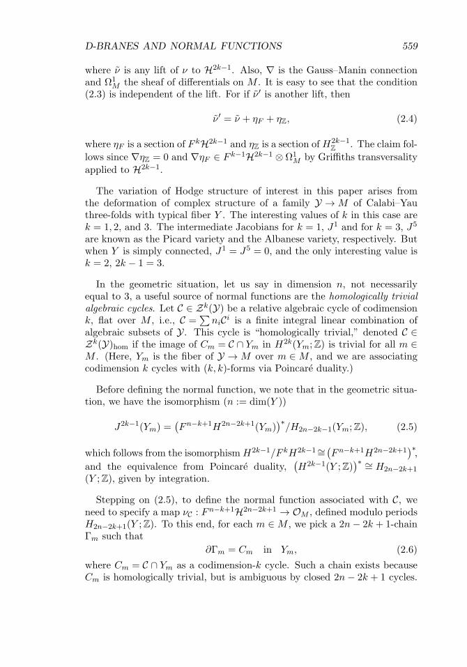
D-BRANES AND NORMAL FUNCTIONS 559
where ν is any lift of ν to H2k−1. Also, ∇ is the Gauss–Manin connectionand Ω1
M the sheaf of differentials on M . It is easy to see that the condition(2.3) is independent of the lift. For if ν ′ is another lift, then
ν ′ = ν + ηF + ηZ, (2.4)
where ηF is a section of F kH2k−1 and ηZ is a section of H2k−1Z
. The claim fol-lows since ∇ηZ = 0 and ∇ηF ∈ F k−1H2k−1 ⊗ Ω1
M by Griffiths transversalityapplied to H2k−1.
The variation of Hodge structure of interest in this paper arises fromthe deformation of complex structure of a family Y → M of Calabi–Yauthree-folds with typical fiber Y . The interesting values of k in this case arek = 1, 2, and 3. The intermediate Jacobians for k = 1, J1 and for k = 3, J5
are known as the Picard variety and the Albanese variety, respectively. Butwhen Y is simply connected, J1 = J5 = 0, and the only interesting value isk = 2, 2k − 1 = 3.
In the geometric situation, let us say in dimension n, not necessarilyequal to 3, a useful source of normal functions are the homologically trivialalgebraic cycles. Let C ∈ Zk(Y) be a relative algebraic cycle of codimensionk, flat over M , i.e., C =
∑niCi is a finite integral linear combination of
algebraic subsets of Y. This cycle is “homologically trivial,” denoted C ∈Zk(Y)hom if the image of Cm = C ∩ Ym in H2k(Ym; Z) is trivial for all m ∈M . (Here, Ym is the fiber of Y → M over m ∈ M , and we are associatingcodimension k cycles with (k, k)-forms via Poincare duality.)
Before defining the normal function, we note that in the geometric situa-tion, we have the isomorphism (n := dim(Y ))
J2k−1(Ym) =(Fn−k+1H2n−2k+1(Ym)
)∗/H2n−2k−1(Ym; Z), (2.5)
which follows from the isomorphism H2k−1/F kH2k−1 ∼=(Fn−k+1H2n−2k+1
)∗,and the equivalence from Poincare duality,
(H2k−1(Y ; Z)
)∗ ∼= H2n−2k+1(Y ; Z), given by integration.
Stepping on (2.5), to define the normal function associated with C, weneed to specify a map νC : Fn−k+1H2n−2k+1 → OM , defined modulo periodsH2n−2k+1(Y ; Z). To this end, for each m ∈ M , we pick a 2n − 2k + 1-chainΓm such that
∂Γm = Cm in Ym, (2.6)
where Cm = C ∩ Ym as a codimension-k cycle. Such a chain exists becauseCm is homologically trivial, but is ambiguous by closed 2n − 2k + 1 cycles.

560 DAVID R. MORRISON AND JOHANNES WALCHER
If we require that Γm depend in a continuous fashion on m, the ambiguityis reduced to H2n−2k+1(Y ; Z).
Now given [ω] ∈ Fn−k+1H2n−2k+1, we can locally on M representing itby a relative 2n − 2k + 1-form ω ∈ Fn−k+1A2n−2k+1 that is closed in thefiber direction and well defined up to the image of dY : Fn−k+1A2n−2k →Fn−k+1A2n−2k+1 (this last assertion follows from the Dolbeault theorem).We then define
νC([ω])m :=∫
Γm
ωm. (2.7)
Let us check that this is well defined. If we choose a different representa-tive ω′ of [ω], the difference is
∫Γm
(ω′m − ωm) =
∫∂Γm
αm, (2.8)
where α ∈ Fn−k+1A2n−2k. This vanishes by type considerations since ∂Γm =Cm is holomorphic, so Poincare dual to a (k, k)-form.
Finally, we check holomorphicity and transversality. Namely, we analyzethe variation of (2.7) as m varies to first order in M . If v is a (not necessar-ily holomorphic) complexified tangent vector to M at m, Kodaira–Spencertheory provides us with a lift, v′, of v to TY. The differential of (2.7) in thedirection of v can be written as
dv(νC([ω]))m = −∫
Cm
(ωm, v′) +∫
Γm
(∇vω)m, (2.9)
where ∇vω represents ∇v[ω] and ∇ is the Gauss–Manin connection onH2n−2k+1.
To check holomorphicity, we let v be anti-holomorphic and [ω] be aholomorphic section of Fn−k+1H2n−2k+1. We then have that ∇v[ω] = 0 inH2n−2k+1. In fact, (∇vω)m = dY (ωm, v′) by Kodaira–Spencer. Thus, (2.9)vanishes, and νC is a holomorphic section of J 2k−1.
To show transversality, we take v to be holomorphic. Note that the state-ment ∇vνC ∈ F k−1H2k−1 is under the isomorphism H2k−1/F k−1H2k−1 ∼=(Fn−k+2H2n−2k+1
)∗ (see (2.5)) equivalent to the assertion that (∇vνC)([ω])m
= 0 for [ω] ∈ Fn−k+2H2n−2k+1, where νC is any lift of νC to(H2n−2k+1
)∗.By the compatibility of the Gauss–Manin connection with Poincare dual-ity, dv(νC([ω]))m = (∇vνC)([ω])m + νC(∇v[ω])m, so this criterion becomesdv(νC([ω]))m = νC(∇v[ω])m, which is already independent of the lift. Now

D-BRANES AND NORMAL FUNCTIONS 561
if [ω] ∈ Fn−k+2H2n−2k+1, (ωm, v′) ∈ Fn−k+1H2n−2k, the first term in (2.9)vanishes by type consideration. This implies transversality.
We close this subsection with one more definition: The association
AJ: Zk(Y)hom → J 2k−1(Y), C → νC (2.10)
is known as the Abel–Jacobi map. It contains some useful information aboutalgebraic cycles and their algebraic equivalences. The theory is particu-larly rich for Calabi–Yau three-folds (as mentioned above, the interestingvalue is then k = 2) and led to a lot of early results on questions relatedto holomorphic curves [35, 41, 42]. That subject was later revolutionized bymirror symmetry and Gromov–Witten theory. As we will try to convey inthis article, normal functions are returning to the enterprise as well, withpromising applications in the context of D-branes and mirror symmetry foropen strings.
2.2 Abel–Jacobi map on the derived category
To explain the relevance of normal functions to D-branes, in general, wetake as starting point Witten’s holomorphic Chern–Simons functional. Wedenote by Y a (compact) Calabi–Yau three-fold, E a holomorphic vec-tor bundle over Y , with ∂ the Dolbeault operator coupled to E. If a ∈A(0,1)(Y,End(E)) is a (0, 1)-form with values in the endomorphisms of E,we define
ShCS(a) =∫
YTr
(12a ∧ ∂a +
13a ∧ a ∧ a
)∧ Ω, (2.11)
where Ω is the (unique up to scale) holomorphic (3, 0)-form on Y . Thefunctional (2.11) was originally proposed in [43], as an expression for thespace-time superpotential in the context of the heterotic string. This pro-posal can be explained on the basis that the critical points of (2.11) areprecisely those a ∈ A(0,1)(Y,End(E)) for which the (0, 2)-part of the curva-ture vanishes,
F (0,2) = ∂a + a ∧ a = 0, (2.12)
i.e., the deformed operator ∂a = ∂ + a is an alternative Dolbeault operatoron E, viewed as a differentiable vector bundle on Y . In general, ∂a willdefine a different complex structure on E.
Witten [10] showed that, in the context of the topological string, thefunctional (2.11) is the target space or string field theory action describing

562 DAVID R. MORRISON AND JOHANNES WALCHER
the tree-level dynamics of open strings on Y coupled to E (a topologicalB-brane). This also led to the suggestion that holomorphic Chern–Simonsshould make sense as a quantum theory, and to various puzzles related tonon-renormalizability of (2.11), appearance of closed strings as intermediatestates, etc. The classical theory has been analyzed in depth over the years(see [44] for a review). The recent results on open–closed topological string[34] can be viewed as giving partial answers to the problems related to thequantum theory.
Connections of the holomorphic Chern–Simons functional with the theoryof normal functions have appeared in the mathematical literature in [45,46] (see also [47]). In the physics literature, a relation to the Abel–Jacobimap for curves on Calabi–Yau three-fold was established, e.g., in [23, 48–50]. When our B-brane, instead of being specified by a holomorphic vectorbundle, is wrapping a holomorphic curve C, it was shown in [23, 49, 50]that the dimensional reduction of the holomorphic Chern–Simons action isnothing but the Abel–Jacobi integral
S(C) =∫
ΓΩ with ∂Γ = C − C0 (2.13)
viewed as a functional on all possible curves homotopic to some given refer-ence holomorphic curve C0.
Neglecting the dynamics of open strings, the most direct physical interpre-tation of the formulas (2.11) and (2.13) is as the tension of BPS domainwallsconnecting the background vacuum (∂ or C0), on the D-brane worldvolume,with some other vacuum, corresponding to a non-trivial critical point, a∗ orC∗, respectively.
T =
{W(a∗) − W(0) = ShCS(a∗),W(C∗) − W(C0) = S(C∗).
(2.14)
It should be clear that, even neglecting open string dynamics, those expres-sions cannot be fully satisfactory for describing the superpotential for anarbitrary B-brane, which might be neither a holomorphic vector bundle nora holomorphic curve in general. The algebraic device needed to generalizethese formulas to an arbitrary object B in Db(Y ) (or some category equiv-alent to it) is the notion of the algebraic second Chern class, calg
2 (B) [51]. Ittakes values in the Chow group CH2(Y ) of algebraic cycles of codimension 2,modulo rational equivalence. The image of calg
2 (B) in cohomology H4(Y ; Z)is equal to the ordinary (topological) second Chern class ctop
2 (B), but calg2 is
generally a more refined invariant.

D-BRANES AND NORMAL FUNCTIONS 563
The algebraic Chern class satisfies axioms very similar to its topologicalcounterpart. In particular, it splits exact triangles in the D-brane category. If
B
�����
����
�
A
����������C
[1]�� (2.15)
for three objects, A, B, and C, then the total Chern classes calg = 1 +∑
calgi
satisfycalg(A) · calg(C) = calg(B), (2.16)
which together with functoriality (and its behavior on holomorphic line bun-dles) is essentially enough to define calg.
Using the algebraic second Chern class puts us directly in the situation dis-cussed in the previous subsection. When ctop
2 (B) = 0 ∈ H4(Y ; Z), the alge-braic cycle defined by calg
2 (B) ∈ CH2(Y ) is homologically trivial and yields,for fixed Y , an Abel–Jacobi class according to the above discussion. WhenB suitably deforms with Y , we obtain a normal function νB = ν
calg2 (B). Inparticular, the formula for the domainwall tension is
T = νB(Ω), (2.17)
where Ω is the same holomorphic three-form as above. It is not hard to seethat this definition reduces to (2.11) and (2.13) when B is a holomorphicvector bundle or a holomorphic curve, respectively.
We should emphasize that the second Chern class will certainly not cap-ture all the intricacies of the superpotential for a general B-brane on aCalabi–Yau. This will require a much more sophisticated analysis, partlyalong the lines of the cited literature.
2.3 Comments on open problems
Before turning to the applications, we will collect a few more remarks fromthe general theory of normal functions, some of which might prove valuablefor further developments.
Extension of Hodge structure
Let (H2k−1Z
, F ∗H2k−1) be an integral variation of Hodge structure of weight2k − 1 over a base M . Let ν be a normal function. In Exercises 1 and 2

564 DAVID R. MORRISON AND JOHANNES WALCHER
in Chapter 7 of [39], it is shown that this data can be used to define anextension of Hodge structure to yield an integral variation of mixed Hodgestructure. At the integral level, this is a locally trivial extension
H2k−1Z
→ (HZ = H2k−1Z
⊕ Z) → Z. (2.18)
The weight filtration is given by W2k−2HZ = 0, W2k−1HZ = H2k−1Z
, W2k =HZ, whereas the Hodge filtration on H = (H2k−1
Z⊕ Z) ⊗ OM is such that it
reduces to the given Hodge filtration F ∗H2k−1 on H2k−1, and to F k+1OM =0, F kOM = OM on the quotient.
In the context of mirror symmetry, a different mixed Hodge structure isrelevant. This mixed Hodge structure is associated with the degenerationat a point of maximal unipotent monodromy in the moduli space [5, 52].The monodromy calculations of [19], partially reviewed in Section 4, areindicative of a very interesting interaction between this limiting mixed Hodgestructure and the one given by extension using the normal function (2.18).It would be interesting to elucidate this further.
More extensions?
We have so far largely suppressed the existence of an A∞-structure on thecategory of B-branes, except to ask the natural question how much of thatstructure is possibly captured by the normal function? In thinking aboutthis problem, we are led to the following speculations.
The A∞-structure on a brane B in the category of B-branes is given bya collection of “higher” products mn satisfying certain conditions of asso-ciativity. At the level of the string worldsheet, the mn with n ≥ 2 can bedetermined by computing the (topological) disk amplitudes with n + 1 openstring insertions on the boundary. m1 is identified with the open stringBRST operator. Finally, m0 is related to the bulk-to-boundary obstructionmap by taking one derivative with respect to the closed string moduli [34].
From general considerations, as well as the identification of the disk ampli-tude with two bulk insertions as the Griffiths infinitesimal invariant [34], itappears natural that the normal function ν can fit as an “m−1” into theA∞-structure. As emphasized in [34], the obstruction map can be inter-preted Hodge theoretically as the dual of the infinitesimal Abel–Jacobi map.Those two observations suggest that one should try to understand whetherthe higher A∞ products mn for n ≥ 1 can also be given a Hodge theoreticinterpretation.

D-BRANES AND NORMAL FUNCTIONS 565
A-model version
All considerations in this paper are phrased in the language of the B-model.On the other hand, we recall that much of the deeper understanding of clas-sical (closed string) mirror symmetry involved the reconstruction of Hodgetheoretic structures in the A-model. In particular, the importance of quan-tum cohomology and the structure of the mirror map become especially clearin the “A-model variation of Hodge structure” [53,54].
It would be very interesting to extend these insights to the open string.A general definition of a functional conjecturally mirror to the holomorphicChern–Simons functional/domainwall tension (see equation (2.14)) is givenin [22], extending [10]. This functional includes corrections from world-sheet instantons (holomorphic disks ending on Lagrangian submanifolds)and should in principle be related to Floer theory and the Fukaya category,as the open string analogues of quantum cohomology. This relation shouldbe similar to that between the holomorphic Chern–Simons functional andthe derived category. In the A-model, the precise relation is not currentlyunderstood, but as an intermediate step, it would be interesting to check atleast the Hodge theoretic statements pertaining to normal functions, basedon, say, axioms for open Gromov–Witten invariants.
3 The real quintic and its mirror
Our interest now turns to the quintic Calabi–Yau X = {G = 0} ⊂ P4, defined
as the vanishing locus of a degree 5 polynomial G in five complex variablesx1, . . . , x5. We assume that X is defined over the reals, which means thatall coefficients of G are real (possibly up to some common phase). The reallocus {xi = xi} ⊂ X is then a Lagrangian submanifold, and after choosing aflat U(1) connection, will define an object in the (derived) Fukaya categoryFuk(X). In this section, we will first review a proposal which identifies a mir-ror object in the category of B-branes of the mirror quintic, in its Landau–Ginzburg description. Via some detours, we will be able to derive from thematrix factorization the corresponding normal function. In the next section,we will then show by an explicit computation that this normal function sat-isfies precisely the inhomogeneous Picard–Fuchs equation proposed in [19].
3.1 Six hundred and twenty-five real quintics
Both the topological type and the homology class in H3(X; Z) of the reallocus depend on the complex structure of X (the choice of (real) polynomial

566 DAVID R. MORRISON AND JOHANNES WALCHER
G). On the other hand, the Fukaya category is independent of the choiceof G (real or not). The object in Fuk(X) that we shall refer to as thereal quintic is defined from the real locus L of X when G is the Fermatquintic G = x5
1 + x52 + x5
3 + x54 + x5
5. It is not hard to see that topologicallyL ∼= RP
3. There are therefore two choices of flat bundles on L, and we willdenote the corresponding objects of Fuk(X) by L+ and L−, respectively.More precisely, since Fuk(X) depends on the choice of a complexified Kahlerstructure on X, we define L± for some choice of Kahler parameter t close tolarge volume Im(t) → ∞, and then continue it under Kahler deformations.In fact, the rigorous definition of the Fukaya category is at present onlyknown infinitesimally close to this large volume point [55]. However, Fuk(X)does exist over the entire stringy Kahler moduli space of X, and at leastsome of the structures vary holomorphically. Our interest here is in thevariation of the categorical structure associated with L± over the entirestringy Kahler moduli space of X, identified via mirror symmetry with thecomplex structure moduli space of the mirror quintic Y .
The Fermat quintic is invariant under more than one anti-holomorphicinvolution. If Z5 denotes the multiplicative group of fifth roots of unity, wedefine for χ = (χ1, . . . , χ5) ∈ (Z5)5 an anti-holomorphic involution σχ of P
4
by its action on homogeneous coordinates
σχ : xi → χixi. (3.1)
The Fermat quintic is invariant under any σχ. The involution and the fixed-point locus only depend on the class of χ in (Z5)5/Z5 ∼= (Z5)4, and we obtainin this way 54 = 625 (pairs of) objects L
[χ]± in Fuk(X). We will return to
those 625 real quintics below, and for the moment focus on L± = L[χ=1]± .
We emphasize again that although we have defined the Lagrangians L[χ]±
as fixed-point sets of anti-holomorphic involutions of the Fermat quintic, wecan think of the corresponding objects of Fuk(X) without reference to thecomplex structure.
3.2 The prediction
The image in K0(Fuk(X)) is the same for L+ and L−. This is the counter-part in the A-model of the triviality of topological Chern classes ctop(B+ −B−) for two objects B± in the category of B-branes. As mentioned above,there should exist a definition of an Abel–Jacobi map to a normal functionof the A-model variation of Hodge structure constructed from the quantumcohomology of X [53,54]. As explained in [19], this normal function can be

D-BRANES AND NORMAL FUNCTIONS 567
realized geometrically by wrapping a D-brane on a disk D whose bound-ary on L represents the non-trivial element of H1(L; Z) ∼= Z2. Neglect-ing instanton corrections, the corresponding truncated normal function ist2 ± 1
4 mod tZ + Z.3 Instanton corrections deform this to
TA(t) =t
2±
(14
+1
2π2
∑d odd
ndqd/2
), (3.2)
where q = e2πit, and nd are the open Gromov–Witten invariants of the realquintic defined in [56], predicted in [19], and fully computed in [22]. Theprecise result for the nd is as follows.
Mirror symmetry for the quintic is governed by the differential operator
L = θ4 − 5z(5θ + 1)(5θ + 2)(5θ + 3)(5θ + 4), (3.3)
where θ = zd/dz. As we will review further below, L is the Picard–Fuchsoperator of the mirror quintic. The equation L�(z) = 0 has four linearlyindependent solutions. Two of those solutions are given by the followingpower-series expansion around z = 0:
�0(z) =∞∑
m=0
(5m)!(m!)5
zm,
�1(z) = �0(z) log z + 5∞∑
m=1
(5m)!(m!)5
zm[Ψ(1 + 5m) − Ψ(1 + m)
],
(3.4)
and determine the mirror map as
t = t(z) =1
2πi�1(z)�0(z)
, q(z) = exp(2πit(z)). (3.5)
The result of [19,22] is
L(�0(z)TA(z)
)=
1516π2
√z. (3.6)
Combined with the boundary conditions (3.2), this is equivalent to
�0(z)TA(z) =�1(z)4πi
+�0(z)
4+
15π2 τ(z), (3.7)
3The sign depends on whether we consider L+ − L− or L− − L+. For this to makesense, note that t
2 − 14 = −( t
2 + 14 ) mod tZ + Z. For details, see [19].

568 DAVID R. MORRISON AND JOHANNES WALCHER
where
τ(z) =Γ(3/2)5
Γ(7/2)
∞∑m=0
Γ(5m + 7/2)Γ(m + 3/2)5
zm+1/2 =√
z +5005
9z3/2 + · · · (3.8)
gives a particular solution of the inhomogeneous Picard–Fuchs equation(3.6).
3.3 Matrix factorization
For the rest of this work, W will denote the one-parameter family of quinticpolynomials
W =15(x5
1 + x52 + x5
3 + x54 + x5
5)
− ψx1x2x3x4x5. (3.9)
Geometrically, the mirror quintic, Y , is the quotient of this one-parameterfamily of quintics by (Z5)3 = (Z5)4/Z5, where (Z5)4 is the group of phasesymmetries of W (for ψ �= 0). Alternatively, we can think of a Landau–Ginzburg orbifold model with worldsheet superpotential W and orbifoldgroup (Z5)4.
We will also have occasion to work in the B-model on the one-parameterfamily of quintic hypersurfaces given by W = 0 in P
4 (without quotient).In this context, we will denote this family by Xψ. When we work in thecontext of the A-model, with an arbitrary complex structure representedby a general quintic polynomial G, we will continue to denote the quinticsimply by X.
Recall that for a quintic X defined by G = 0, the homological Calabi–Yau/Landau–Ginzburg correspondence [57–60] states that the derived cat-egory of coherent sheaves of X is equivalent to the graded, equivariantcategory of matrix factorizations of the corresponding Landau–Ginzburgsuperpotential,
Db(X) = MF(G/Z5), (3.10)where Z5 is the diagonal group of phase symmetries. The analogous state-ment for the mirror quintic is
Db(Y ) ∼= MF(W/Z45) (3.11)
with (Z5)4 as above.
To describe an object mirror to the real quintic, we begin with findinga matrix factorization of the one-parameter family of superpotentials (3.9).
D-BRANES AND NORMAL FUNCTIONS 569
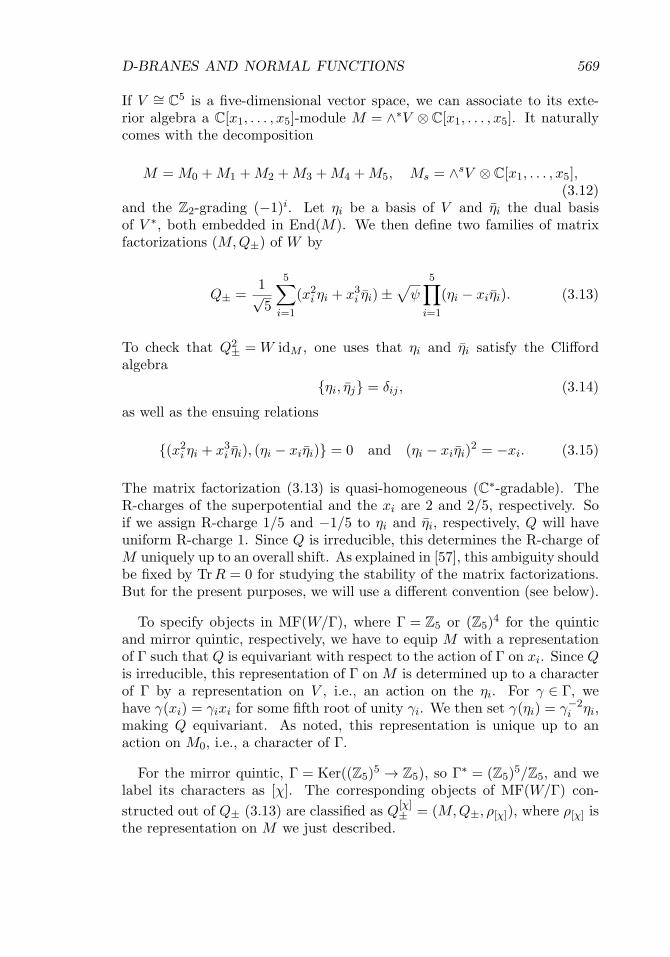
If V ∼= C5 is a five-dimensional vector space, we can associate to its exte-
rior algebra a C[x1, . . . , x5]-module M = ∧∗V ⊗ C[x1, . . . , x5]. It naturallycomes with the decomposition
M = M0 + M1 + M2 + M3 + M4 + M5, Ms = ∧sV ⊗ C[x1, . . . , x5],(3.12)
and the Z2-grading (−1)i. Let ηi be a basis of V and ηi the dual basisof V ∗, both embedded in End(M). We then define two families of matrixfactorizations (M, Q±) of W by
Q± =1√5
5∑i=1
(x2i ηi + x3
i ηi) ±√
ψ
5∏i=1
(ηi − xiηi). (3.13)
To check that Q2± = W idM , one uses that ηi and ηi satisfy the Clifford
algebra
{ηi, ηj} = δij , (3.14)
as well as the ensuing relations
{(x2i ηi + x3
i ηi), (ηi − xiηi)} = 0 and (ηi − xiηi)2 = −xi. (3.15)
The matrix factorization (3.13) is quasi-homogeneous (C∗-gradable). TheR-charges of the superpotential and the xi are 2 and 2/5, respectively. Soif we assign R-charge 1/5 and −1/5 to ηi and ηi, respectively, Q will haveuniform R-charge 1. Since Q is irreducible, this determines the R-charge ofM uniquely up to an overall shift. As explained in [57], this ambiguity shouldbe fixed by TrR = 0 for studying the stability of the matrix factorizations.But for the present purposes, we will use a different convention (see below).
To specify objects in MF(W/Γ), where Γ = Z5 or (Z5)4 for the quinticand mirror quintic, respectively, we have to equip M with a representationof Γ such that Q is equivariant with respect to the action of Γ on xi. Since Qis irreducible, this representation of Γ on M is determined up to a characterof Γ by a representation on V , i.e., an action on the ηi. For γ ∈ Γ, wehave γ(xi) = γixi for some fifth root of unity γi. We then set γ(ηi) = γ−2
i ηi,making Q equivariant. As noted, this representation is unique up to anaction on M0, i.e., a character of Γ.
For the mirror quintic, Γ = Ker((Z5)5 → Z5), so Γ∗ = (Z5)5/Z5, and welabel its characters as [χ]. The corresponding objects of MF(W/Γ) con-structed out of Q± (3.13) are classified as Q
[χ]± = (M, Q±, ρ[χ]), where ρ[χ] is
the representation on M we just described.

570 DAVID R. MORRISON AND JOHANNES WALCHER
Conjecture: There is an equivalence of categories Fuk(X) ∼= MF(W/
(Z5)4) which identifies the 625 pairs of objects L[χ]± with the 625 pairs of
equivariant matrix factorizations Q[χ]± .
Note: One can formulate a similar conjecture for any hypersurface inweighted projective space which has a Fermat point in its complex structuremoduli space.
3.4 Intersection index
The first piece of evidence for the above conjecture comes from Ref. [61].In that paper, the 625 Lagrangian submanifolds of X described above wereassociated with the so-called L = (1, 1, 1, 1, 1) A-type Recknagel–Schomerusstates in the Gepner model. These A-type boundary states had been con-structed in [62] as tensor products of Cardy states in the N = 2 minimalmodel building blocks of the Gepner model. In turn, these Cardy statesof the minimal model were identified in [63] with the Lagrangian wedgebranes of opening angle 4π/5 in the Landau–Ginzburg description of theN = 2 minimal models. Via mirror symmetry for the minimal models, thosewedges are equivalent to the matrix factorizations based on x5
i = x2i x
3i (see,
e.g., [64]). These are precisely the building blocks of the factorization (3.13),specialized to ψ = 0. The above deformation away from ψ = 0, as well asthe identification of the pairs Q
[χ]± with the pairs of objects L
[χ]± , was first
noted in [65], following the suggestion of [61].
The initial step in the above identification of L[χ]± with Q
[χ]± was justified
in [61] by a comparison of the intersection indices of the L[χ]± with the cor-
responding intersection indices of the Gepner model boundary states. Wewill reproduce this here using the matrix factorizations. The match of thedomainwall tensions4 L+ − L− and Q+ − Q− computed in the A-model andB-model, respectively, constitutes further evidence for the above conjecture.
Let us start with the geometric intersection index between5 L[χ] and L[χ′].Because of the projective equivalence, we have to look at the intersectionof the fixed-point loci of σχ and σωχ′ from (3.1) where ω runs over the five
4Note that because of the symmetries, these domainwall tensions do not depend on thediscrete group representation.
5The intersection index, being topological, does not depend on the Wilson lines on theA-branes. For the B-branes, it is correspondingly independent of the sign of the squareroot in (3.13).

D-BRANES AND NORMAL FUNCTIONS 571
fifth roots of unity. It is not hard to see that topologically
Fix(σχ) ∩ Fix(σωχ′) ∩ X ∼= RPd−2, d = #{χ′
i = ωχi}. (3.16)
After making the intersection transverse by a small deformation in the nor-mal direction, we obtain a vanishing contribution for d = 0, 1, 3, 5, and ±1for d = 2, 4, where the sign depends on the non-trivial phase differencesχ∗
i ωχ′i. Explicitly, one finds
L[χ] ∩ L[χ′] =∑ω∈Z5
f1(χ′∗ωχ), (3.17)
where
f1(χ) =
⎧⎪⎨⎪⎩
5∏i=1
sgn(Im(χi)
), if #{i, χi = 1} = 2, 4,
0 else.
(3.18)
To compute the intersection index between the matrix factorizations, we usethe index theorem of [57]. It says in general
χ Hom((M, Q, ρ), (M ′, Q′, ρ′)
):=
∑i
(−1)i dim Homi((M, Q, ρ), (M ′, Q′, ρ′)
)
=1
|Γ|∑γ∈Γ
StrM ′ ρ′(γ)∗ 1∏5i=1(1 − γi)
StrM ρ(γ),
(3.19)
where γi are the eigenvalues of γ ∈ Γ acting on xi, and ρ and ρ′ are therepresentations of Γ on M . For M = M ′, Q = Q′, and ρ = ρ[χ], and ρ′ = ρ[χ′]described above, this evaluates to
− 154
∑γ∈(Z5)4
χ(γ′)∗χ(γ)5∏
i=1
(γi + γ2i − γ3
i − γ4i ) = −
∑ω∈Z5
f2(χ′∗ωχ), (3.20)
where
f2(χ) =
⎧⎪⎨⎪⎩
5∏i=1
sgn(Im(χi)
), if #{i, χi = 1} = 0
0 else.
(3.21)
We do not know any generally valid result from the representation theoryof finite cyclic group which shows that (3.17) and (3.20) coincide. It is,

572 DAVID R. MORRISON AND JOHANNES WALCHER
however, not hard to check by hand or computer that for all χ,
∑ω∈Z5
(f1 + f2)(ωχ) = 0. (3.22)
HenceL[χ] ∩ L[χ′] = χ Hom(Q[χ], Q[χ′]) (3.23)
as claimed.
3.5 Bundles
We now proceed with the construction of the normal function from thematrix factorization (3.13). To this end, we use the homological Calabi–Yau/Landau–Ginzburg correspondence (3.10) for the quintic as describedin [60]. This will produce for us a set of five complexes of coherent sheaves(bundles) on the one-parameter family of quintics Xψ. By making thoseequivariant with respect to the geometric (Z5)3 action (thus implementing(3.11)) will yield the 625 objects in Db(Y ) mirror to the real quintics.
The technique underlying the algorithm of [60] is the gauged linear sigmamodel of [66]. Thus, we first construct a D-brane in the gauged linear sigmamodel from the equivariant matrix factorization, and in the second step acomplex of (line) bundles on the quintic. We have to and can live with twoambiguities in the construction. The first ambiguity is the Landau–Ginzburgmonodromy (cyclic permutation of the characters of Γ = Z5), whereas thesecond depends on a certain “band restriction rule” for assignment of thegauge charges in the linear sigma model. The upshot of the construction isthe following. We can view the matrix factorization, namely the Z2-gradedmodule M equipped with Q of Q2 = W as a 2-periodic infinite complex overthe affine singularity W = 0. We then truncate this infinite complex to asemi-infinite complex in a way that depends on the charge and representa-tion assignments in the gauged linear sigma model. The departure of thisconstruction from the traditional (Serre) correspondence between sheaveson the hypersurface and graded modules on the affine singularity is that thecohomological grading of the complexes also depends on the linear sigmamodel charges. We now implement this algorithm in our example, referringto [60] for the complete details.
Given (M, Q, ρχ), we first assign R-charges (i.e., a C∗-representation, gen-
erated by a rational Hermitian matrix, R on M) in such a way that
eiπR = ρχ(γ)(−1)s, (3.24)

D-BRANES AND NORMAL FUNCTIONS 573
where (−1)s is the Z2-grading on M and γ ≡ e2πi/5 is the generator of Z5.In the decomposition (3.12), ρχ(γ) = e2πi(n−2s)/5, where χ = e2πin/5. Wechoose the R-charge assignment of Ms in (3.12) as Rs = s
5 + 2n5 .
Following the algorithm of [60], we now select a “band” of five consecutiveintegers Λ = {0, 1, 2, 3, 4} and find for each s an integer Rs = s mod 2 andan integer qs ∈ Λ such that
Rs = Rs − 2qs
5. (3.25)
Rs and qs are uniquely determined by this equation. Depending on n, wefind for the pairs (Rs, qs) the following table:
������sn 0 1 2 3 4
0 (0, 0) (2, 4) (2, 3) (2, 2) (2, 1)1 (1, 2) (1, 1) (1, 0) (3, 4) (3, 3)2 (2, 4) (2, 3) (2, 2) (2, 1) (2, 0)3 (1, 1) (1, 0) (3, 4) (3, 3) (3, 2)4 (2, 3) (2, 2) (2, 1) (2, 0) (4, 4)5 (1, 0) (3, 4) (3, 3) (3, 2) (3, 1)
(3.26)
This data yields a graded, gauge-invariant matrix factorization, QGLSM ofthe linear sigma model superpotential WGLSM = PW , where P is Witten’sP-field [66]. In reducing to the non-linear sigma model on the hypersurface,the bulk modes of P are integrated out, while the quantization of the singleboundary degree of freedom yields the Fock space of a harmonic oscillator,HP ∼= ⊕N≥0HP
N , where each HPN
∼= C. The resulting complex on the quintichypersurface is built from the tensor product M ⊗ HP , where Ms ⊗ HP
N isplaced in homological degree d = Rs + 2N and twisted by the line bundleO(qs + 5N). The original matrix factorization Q acts on this complex in away compatible with all gradings.
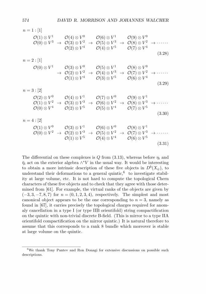
For the data above, we obtain explicitly the following five complexes(here, V s ≡ ∧sV , and the integer in square brackets indicates the homo-logical degree of the first term in the complex):
n = 0 : [0]
O(0) ⊗ V 0
→O(2) ⊗ V 1
O(1) ⊗ V 3
O(0) ⊗ V 5→
O(5) ⊗ V 0
O(4) ⊗ V 2
O(3) ⊗ V 4→
O(7) ⊗ V 1
O(6) ⊗ V 3
O(5) ⊗ V 5→ · · · · · ·
(3.27)
574 DAVID R. MORRISON AND JOHANNES WALCHER
n = 1 : [1]
O(1) ⊗ V 1
O(0) ⊗ V 3 →O(4) ⊗ V 0
O(3) ⊗ V 2
O(2) ⊗ V 4→
O(6) ⊗ V 1
O(5) ⊗ V 3
O(4) ⊗ V 5→
O(9) ⊗ V 0
O(8) ⊗ V 2
O(7) ⊗ V 4→ · · · · · ·
(3.28)
n = 2 : [1]
O(0) ⊗ V 1
→O(3) ⊗ V 0
O(2) ⊗ V 2
O(1) ⊗ V 4→
O(5) ⊗ V 1
O(4) ⊗ V 3
O(3) ⊗ V 5→
O(8) ⊗ V 0
O(7) ⊗ V 2
O(6) ⊗ V 4→ · · · · · ·
(3.29)
n = 3 : [2]
O(2) ⊗ V 0
O(1) ⊗ V 2
O(0) ⊗ V 4→
O(4) ⊗ V 1
O(3) ⊗ V 3
O(2) ⊗ V 5→
O(7) ⊗ V 0
O(6) ⊗ V 2
O(5) ⊗ V 4→
O(9) ⊗ V 1
O(8) ⊗ V 3
O(7) ⊗ V 5→ · · · · · ·
(3.30)
n = 4 : [2]
O(1) ⊗ V 0
O(0) ⊗ V 2 →O(3) ⊗ V 1
O(2) ⊗ V 3
O(1) ⊗ V 5→
O(6) ⊗ V 0
O(5) ⊗ V 2
O(4) ⊗ V 4→
O(8) ⊗ V 1
O(7) ⊗ V 3
O(6) ⊗ V 5→ · · · · · ·
(3.31)
The differential on these complexes is Q from (3.13), whereas before ηi andηi act on the exterior algebra ∧∗V in the usual way. It would be interestingto obtain a more intrinsic description of these five objects in Db(Xψ), tounderstand their deformations to a general quintic,6 to investigate stabil-ity at large volume, etc. It is not hard to compute the topological Cherncharacters of these five objects and to check that they agree with those deter-mined from [61]. For example, the virtual ranks of the objects are given by(−3, 3,−7, 8, 7) for n = (0, 1, 2, 3, 4), respectively. The simplest and mostcanonical object appears to be the one corresponding to n = 3, namely asfound in [67], it carries precisely the topological charges required for anom-aly cancellation in a type I (or type IIB orientifold) string compactificationon the quintic with non-trivial discrete B-field. (This is mirror to a type IIAorientifold compactification on the mirror quintic.) It is natural therefore toassume that this corresponds to a rank 8 bundle which moreover is stableat large volume on the quintic.
6We thank Tony Pantev and Ron Donagi for extensive discussions on possible suchdescriptions.

D-BRANES AND NORMAL FUNCTIONS 575
3.6 From matrix factorization to curve
The five complexes in the previous subsection define five objects in Db(Xψ).(Although semi-infinite, they are quasi-isomorphic to finite complexesbecause of the eventual periodicity.) As discussed before, to obtain the 625objects in Db(Y ) mirror to the real quintics, we have to make these objects(Z5)3 equivariant. It would be interesting to understand this construction indetail and, in particular, what happens under the resolution of the orbifoldsingularities. For our purposes, however, we do not need this. In fact, tocompute the normal function by the Abel–Jacobi map, we do not even needto distinguish between the five objects on the quintic. Note that the definingsemi-infinite complexes differ only in low homological degree by extensionsby line bundles, which contribute only trivially to algebraic K-theory and theAbel–Jacobi map. In other words, all the information about the normal func-tion is contained in the 2-periodic part of the complexes, which is nothing butthe original matrix factorization! This fact would have allowed us to bypassall the complications associated with the homological Calabi–Yau/Landau–Ginzburg correspondence. We nevertheless presented the detailed results inthe previous subsection, because we feel that they might be of independentinterest, for instance, for questions of stability.
In this subsection, we proceed with the computation of the algebraicsecond Chern classes of Q
[χ]ε , where ε = ±1. Specifically, the domainwall
tension of our interest is given by the image under the Abel–Jacobi mapof Q
[χ]+ − Q
[χ]− . Note that this is well defined since, as follows, e.g., from
the index theorem (3.19), the topological Chern classes only depend on χ,and not on ε, which is the sign of the square root in (3.13). On the otherhand, the Abel–Jacobi map is independent of χ, as explained in the previousparagraph.
It does, however, make a difference whether we work on the quintic or itsmirror. On the quintic, we can work with the explicit bundle representativesfrom (3.30). Let
E± = Ker(O(2) ⊕ O(1)10 ⊕ O(0)5
Q±−→ O(4)5 ⊕ O(3)10 ⊕ O(2)). (3.32)
In general, for a bundle of rank r with sufficiently many sections, one candetermine the second Chern class by choosing r − 1 generic sections andfinding the codimension-2 locus where those sections fail to be linearly inde-pendent. Since twisting by O(1) will alter the image in the Chow grouponly trivially, we can always arrange for sufficiently many sections by twist-ing with O(n) for n large enough. For bundles such as E±(n), we can

576 DAVID R. MORRISON AND JOHANNES WALCHER
conveniently find sections7 by using the 2-periodicity of the complex (3.30)as the image of Q in the previous step. In the case at hand, we select sevencolumns of the matrix representation of (3.30) and study the ideal generatedby the minors of the resulting 7 × 16-dimensional matrix.
After some algebra, we find that the second Chern classes can be repre-sented as
c2(E+) − c2(E−) = [C+ − C−] ∈ CH2(Xψ), (3.33)
where C± stands for the algebraic curve
C± = {x1 + x2 = 0, x3 + x4 = 0, x25 ±
√5ψx1x3 = 0} ⊂ Xψ. (3.34)
Of course, we are really interested in the matrix factorizations and cor-responding bundles as objects in Db(Y ), where Y = Xψ/(Z5)3 is the mirrorquintic. Their second Chern classes take values in CH2(Y ) and can bedescribed by considering the image of C± under the (Z5)3 orbifold group.We will study this quotient procedure carefully in the following section.
4 Main computation
As before, we let Xψ be the one-parameter family of quintics given by (3.9).The intersection of Xψ with the plane P = {x1 + x2 = x3 + x4 = 0} is aplane curve of degree 5 which is reducible, with three components (see leftpart of figure 1). One component is the line x5 = 0, the other two are conicsC± described by (3.34). Obviously, [C+ − C−] = 0 ∈ H2(Xψ) for all ψ, andthus the cycle C+ − C− defines a normal function ν for the one-parameterfamily of quintics Xψ. Consequently, we also obtain a pair of curves and anormal function for the mirror quintic Y , which we will denote by the samesymbols. Now pick a family of three-chains Γ ⊂ Y with ∂Γ = C+ − C−. Thedomainwall tension or truncated normal function is given by
TB = TB(z) =∫
ΓΩ, (4.1)
where Ω is a particular choice of holomorphic three-form on Y , furtherspecified below.
7This was initially suggested to us by Nick Warner and anticipated also by Duco vanStraten.
D-BRANES AND NORMAL FUNCTIONS 577
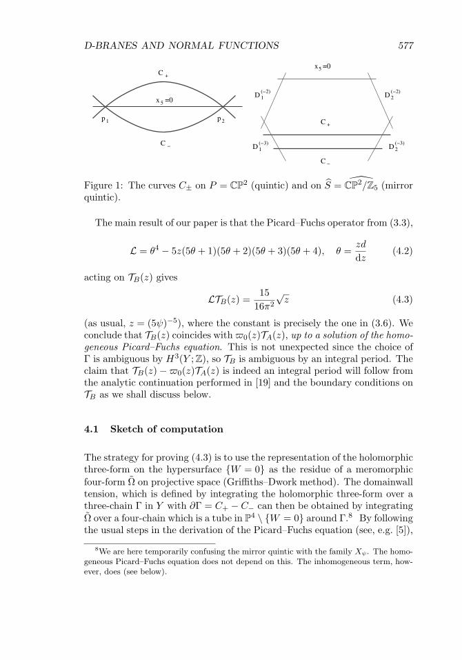
Figure 1: The curves C± on P = CP2 (quintic) and on S =
CP2/Z5 (mirror
quintic).
The main result of our paper is that the Picard–Fuchs operator from (3.3),
L = θ4 − 5z(5θ + 1)(5θ + 2)(5θ + 3)(5θ + 4), θ =zd
dz(4.2)
acting on TB(z) gives
LTB(z) =15
16π2
√z (4.3)
(as usual, z = (5ψ)−5), where the constant is precisely the one in (3.6). Weconclude that TB(z) coincides with �0(z)TA(z), up to a solution of the homo-geneous Picard–Fuchs equation. This is not unexpected since the choice ofΓ is ambiguous by H3(Y ; Z), so TB is ambiguous by an integral period. Theclaim that TB(z) − �0(z)TA(z) is indeed an integral period will follow fromthe analytic continuation performed in [19] and the boundary conditions onTB as we shall discuss below.
4.1 Sketch of computation
The strategy for proving (4.3) is to use the representation of the holomorphicthree-form on the hypersurface {W = 0} as the residue of a meromorphicfour-form Ω on projective space (Griffiths–Dwork method). The domainwalltension, which is defined by integrating the holomorphic three-form over athree-chain Γ in Y with ∂Γ = C+ − C− can then be obtained by integratingΩ over a four-chain which is a tube in P
4 \ {W = 0} around Γ.8 By followingthe usual steps in the derivation of the Picard–Fuchs equation (see, e.g. [5]),
8We are here temporarily confusing the mirror quintic with the family Xψ. The homo-geneous Picard–Fuchs equation does not depend on this. The inhomogeneous term, how-ever, does (see below).

578 DAVID R. MORRISON AND JOHANNES WALCHER
the action of L on the domainwall tension can be reduced to a boundaryterm consisting of the integral of certain meromorphic three-forms over atube around the boundary curves C±. To be specific, let us consider thecontribution from C+. The main observation that will make the computationpossible is the following.
The curve C+ lies in the plane P = {x1 + x2 = x3 + x4 = 0}. There-fore, if we could fit the tube around C+ completely inside P , the integralover it of any meromorphic three-form with poles on W = 0 would van-ish. The reason we cannot restrict the computation to P is of course thatP ∩ {W = 0} contains not just C+, but also C−, as well as the line x5 = 0,so that a tube around C+ inside P will intersect one of the other compo-nents, hence Xψ. But then, we can fit the tube around C+ into P except fora small neighborhood of the points where the components of P ∩ {W = 0}meet. There are two such points, p1 = {x1 = −x2, x3 = x4 = x5 = 0} andp2 = {x1 = x2 = x5 = 0, x3 = −x4}, and the computation can be localizedto a small neighborhood of p1 and p2, which fit entirely inside an affinepatch.
There is, however, an important subtlety in performing this computationas we have just sketched.9 Namely, the intersection points p1 and p2 areactually singular points of the mirror quintic, and these singularities must beresolved first in order to perform the computation. Recall that resolving thesingularities amounts to varying the Kahler class on the quintic mirror toa generic value; since the inhomogeneous Picard–Fuchs equation should beindependent of the Kahler class, it will not matter how we do the resolutionof singularities.
4.2 Resolution of singularities
Since the plane P = {x1 + x2 = x3 + x4 = 0} itself plays an important rolein the computation, we also need to resolve singularities that appear on itafter passing to the quotient. The symmetry group (Z5)3 permutes 25 · 5!
2!2! =750 similar planes, but a Z5 subgroup preserves our plane, with a generatoracting via
(x1,−x1, x3,−x3, x5) −→ (x1,−x1, e2πi/5x3,−e2πi/5x3, e−4πi/5x5).
This group action has three fixed points, at p1, p2, and (0, 0, 0, 0, 1), and thefirst two of these must be resolved.10
9We can attest to the fact that if this subtlety is ignored, a wrong answer is obtained!10The third point does not lie on the quintic mirror for generic ψ and hence need not
be resolved.
D-BRANES AND NORMAL FUNCTIONS 579
These singularities on S = P/Z5 are Hirzebruch–Jung singularities [68,69]
and can be resolved by classical methods11 to obtain a surface S = CP
2/Z5.The result is that each singular point pi is replaced by two rational curvesD
(−2)i and D
(−3)i , in the configuration shown in figure 1. We denote the
intersections of (the transforms of) C± with the curve D(−3)i by pi,±.
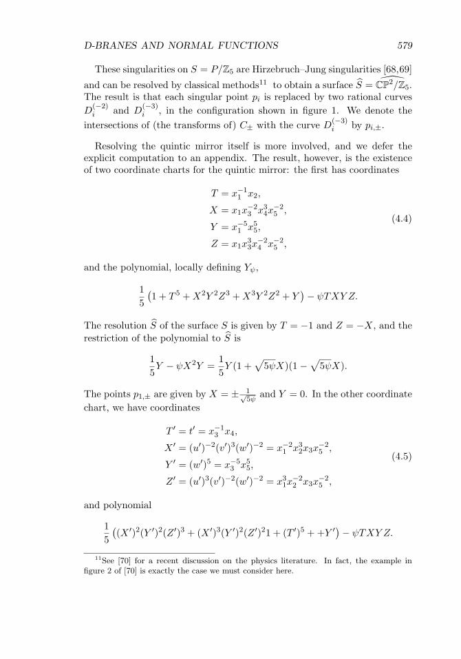
Resolving the quintic mirror itself is more involved, and we defer theexplicit computation to an appendix. The result, however, is the existenceof two coordinate charts for the quintic mirror: the first has coordinates
T = x−11 x2,
X = x1x−23 x3
4x−25 ,
Y = x−51 x5
5,
Z = x1x33x
−24 x−2
5 ,
(4.4)
and the polynomial, locally defining Yψ,
15
(1 + T 5 + X2Y 2Z3 + X3Y 2Z2 + Y
)− ψTXY Z.
The resolution S of the surface S is given by T = −1 and Z = −X, and therestriction of the polynomial to S is
15Y − ψX2Y =
15Y (1 +
√5ψX)(1 −
√5ψX).
The points p1,± are given by X = ± 1√5ψ
and Y = 0. In the other coordinatechart, we have coordinates
T ′ = t′ = x−13 x4,
X ′ = (u′)−2(v′)3(w′)−2 = x−21 x3
2x3x−25 ,
Y ′ = (w′)5 = x−53 x5
5,
Z ′ = (u′)3(v′)−2(w′)−2 = x31x
−22 x3x
−25 ,
(4.5)
and polynomial
15
((X ′)2(Y ′)2(Z ′)3 + (X ′)3(Y ′)2(Z ′)21 + (T ′)5 + +Y ′) − ψTXY Z.
11See [70] for a recent discussion on the physics literature. In fact, the example infigure 2 of [70] is exactly the case we must consider here.

580 DAVID R. MORRISON AND JOHANNES WALCHER
The resolution S of the surface S is given by T ′ = −1 and Z ′ = −X ′, andthe restriction of the polynomial to S is
15Y ′ − ψ(X ′)2Y ′ =
15Y ′(1 +
√5ψX ′)(1 −
√5ψX ′).
The points p2,± are given by X ′ = ± 1√5ψ
and Y ′ = 0.
4.3 Inhomogeneous Picard–Fuchs via Griffiths–Dwork
Let us recall our conventions. We have
W =15(x5
1 + x52 + x5
3 + x54 + x5
5)
− ψx1x2x3x4x5, (4.6)
and z = (5ψ)−5. To derive the Picard–Fuchs equations by the Griffiths–Dwork method, we introduce the four-form on P
4,
ω =∑
i
(−1)i−1xi dx1 ∧ . . . ∧ dxi ∧ . . . ∧ dx5, (4.7)
as well as the contraction of ω with the tangent vectors ∂i (i = 1, . . . , 5)
ωi = ω(∂i). (4.8)
A convenient choice of gauge for the holomorphic three-form is
Ω(z) = ResW=0 Ω(z), Ω(z) :=ω
W (z). (4.9)
Traditionally, one derives the Picard–Fuchs equation by working with theexpression (4.9), thought of as living on the quintic Xψ. The holomorphicthree-form on the mirror quintic Y can be obtained by pulling back (4.9)in local patches via blowup maps such as described in the appendix. Forordinary periods, the net effect of the quotient by (Z5)3 is then simply anadditional normalization factor of 5−3 [4]. Such a simple relation is notexpected to hold for generic normal functions, so we need to evaluate thingsmore carefully.

D-BRANES AND NORMAL FUNCTIONS 581
Following the reduction of pole algorithm of Griffiths and keeping trackof exact pieces, we find with the above definitions,
LΩ :=((1 − ψ5)∂4
ψ − 10ψ4∂3ψ − 25ψ3∂2
ψ − 15ψ2∂ψ − 1)Ω = −dβ, (4.10)
where the exact piece is
β =3!
W 4
(x4
2x43x
44x
45ω1 + ψx2x
53x
54x
55ω2 + ψ2x1x2x
23x
64x
65ω3
+ ψ3x21x
22x
23x
34x
75ω4 + ψ4x3
1x32x
33x
34x
45ω5
)
+2
W 3
(ψx3x
54x
55ω3 + 3ψ2x1x2x3x
24x
65ω4 + 6ψ3x2
1x22x
23x
24x
35ω5
)
+1
W 2
(ψx4x
55ω4 + 7ψ2x1x2x3x4x
25ω5
)
+1W
(ψx5ω5
).
(4.11)
Now the standard Picard–Fuchs operator L from (3.3) is related to L from(4.10) by
L = − 154 L 1
ψ. (4.12)
On the other hand, the normalization of the holomorphic three-form inwhich the solutions (3.4) correspond to primitive integral periods of themirror quintic is [4]
Ω =( 5
2πi
)3ψ Ω =
( 52πi
)3ψ ResW=0
ω
W. (4.13)
The domainwall tension for which we claim (4.3) is defined by
TB(z) =∫
ΓΩ(z), (4.14)
where Γ is any three-chain in Y with ∂Γ = C+ − C−. Let Tε(Γ) be a smalltube around Γ of size ε > 0. Then by (4.9),
∫Γ
Ω =1
2πi
∫Tε(Γ)
Ω. (4.15)
By combining this with (4.12) and (4.13), the claim (4.3) takes the form
L∫
Tε(Γ)Ω = − 3π2
51/2ψ5/2 , (4.16)
which we now proceed to show.

582 DAVID R. MORRISON AND JOHANNES WALCHER
There are two types of contributions to the RHS of (4.16), depending onwhether the derivatives in L act on the chain or on Ω. When L acts entirelyon Ω, we use (4.10) and obtain the boundary term
−∫
Tε(C+−C−)β. (4.17)
We will see below that this in fact gives the entire contribution claimedin (4.16). To show that the contributions from derivatives acting on Tε(Γ)vanish, we use the fact that as ψ varies, the three-chain Γ changes to firstorder only at its boundary, in a way dictated by the dependence of C± onψ. Namely, the first-order variation of C± is a section n ∈ NC±/Y of thenormal bundle of C± in Y . This normal vector lifts to the tube Tε(C±) andwe shall show below that for l = 0, 1, 2, 3,
∫Tε(C+−C−)
(x1x2x3x4x5)lω(n)W l+1 = 0, (4.18)
where ω(n) is the contraction of ω with the normal vector n. Establishingthis claim together with the fact that (4.17) evaluates to the RHS of (4.16)will complete the proof.
As described in Section 4.1, we can evaluate integrals of meromorphicthree-forms over Tε(C±) as in (4.17) and (4.18), by laying the tube intothe plane P (or rather its resolution S) outside a small neighborhood ofthe points pi,±. In those neighborhoods, we can use the coordinates ofSection 4.2. Consider p1,+, with coordinates (4.4). The curve C+ is givenby T = −1, X = −Z = 1/
√5ψ, and locally parametrized by
Y = r eiϕ (4.19)
varying in a neighborhood of r = 0. Our tube Tε(C+) is defined by pickinga C∞ normal vector v which satisfies dvW �= 0 on C+ and points inside ofP outside of a small neighborhood of Y = 0. To this end, let f(r) be anon-negative C∞ function with f(0) = 1 and f(r) = 0 for r ≥ r∗ > 0. Wethen choose
v =f(r)
1 + (Y/5)∂T − e−iϕ∂X + e−iϕ∂Z . (4.20)
Clearly, v points inside of P for r > r∗ and one easily checks
dvW |C+ = f(r) + 2√
ψ5 r > 0 for 0 ≤ r ≤ 2r∗. (4.21)
(We are here assuming that ψ > 0. This is no restriction as long as ψ �= 0.)So the part of the tube Tε(C+; p1,+) around C+ which is close to p1,+ is

D-BRANES AND NORMAL FUNCTIONS 583
parametrized as
T = −1 + εeiχ f(r)1 + Y
5
, X = −Z =1√5ψ
− εeiχe−iϕ, (4.22)
0 ≤ χ < 2π, 0 ≤ ϕ < 2π, 0 ≤ r < 2r∗. (4.23)
(In all of this, we should really be taking the limit ε → 0, but the result willturn out to be independent of ε.) There is then a corresponding piece of thetube around p2,+. The part of the tube in between does not matter as it liesentirely within P , so any meromorphic three-form vanishes there. Finally,the contribution from C− will come from substituting
√ψ → −
√ψ in the
final answer.
We now apply the coordinate transformation (4.4) to evaluate the three-forms ωi on the tube (4.22). Choosing x1 = 1, we have
ω1 = −x2 dx3 dx4 dx5 + x3 dx2 dx4 dx5 − x4 dx2 dx3 dx5 + x3 dx2 dx3 dx4,
ω2 = dx3 dx4 dx5,
ω3 = − dx2 dx4 dx5,
ω4 = dx2 dx3 dx5,
ω5 = − dx2 dx3 dx4,(4.24)
and
dx2
x2=
dT
T,
dx3
x3=
35
dZ
Z+
25
dX
X+
25
dY
Y,
dx4
x4=
35
dX
X+
25
dZ
Z+
25
dY
Y,
dx5
x5=
15
dY
Y.
(4.25)
After restricting to X = −Z, this yields ω1 = ω2 = ω5 = 0 and
ω3 = ω4 = dx2 dx3 dx5 =x2x3x5
5TXYdT dX dY. (4.26)
Substituting (4.22), we obtain
dT dX dY = ε2e2iχ f
1 + (Y/5)
(rf ′
f− 1
)dχ dϕ dr, (4.27)

584 DAVID R. MORRISON AND JOHANNES WALCHER
where f ′ =df/dr. The procedure to compute integrals of the forms p dx2 dx3dx5/W l+1, where p is some monomial in xi’s, over the tube Tε(C+; p1,+) isto first write a Laurent series in powers of εeiχ and eiϕ. Integration over χand ϕ will then retain only terms of order e0iχ and e0iϕ, respectively. Finally,we will do the integral over r.
To begin with, on the tube we have the expansion
W = ε
(f + 2
√ψ5 r
)− ε2
(2f2 + 2
√ψ5 f r + ψre−iϕ
)
+ ε3(2f3 + ψfre−iϕ
)+ O(ε4), (4.28)
where ε = εeiχ and f = f/(1 + (Y/5)). In (4.28), we have truncated to orderε3 since ω3 ∝ ε2, and the highest power of W of interest corresponds to l = 3.
Let us consider the computation of a sample term in β from (4.11).Expanding in ε, we have
ψx4x55ω4
W 2 =
(−
√ψ5 eiϕr
rf ′ − f
1 + (Y/5)
(f + 2
√ψ5 r
)−2
+ O(ε)
)dχ dϕ dr.
(4.29)The integration over ϕ clearly kills this term. In fact, it turns out that allthe terms in β which do not already vanish after restricting to Tε(C+; p1)give zero after integration over χ and ϕ.
Going to p2,+, where the local coordinates of (4.5) can be accomplishedin the above formulas by exchanging x3 with x1 and x4 with x2. There arethen only two terms to consider.
• The term 6x42x
43x
44x
45ω1/W 4 gives, after integration over χ and ϕ,
(2π)212(rf ′ − f)r2
[ψr2 + 4
√5ψrf + 15f2
125ψ(f + 2
√(ψ/5)r
)6
]. (4.30)
Integration over r then gives
3π2
2√
5ψ5/2. (4.31)
• The term 6ψx2x53x
54x
55ω2/W 4 gives some complicated expression after
integration over the angles, but the integral over r vanishes.
D-BRANES AND NORMAL FUNCTIONS 585
Taking into account the contribution from C−, the final result for(4.17) is
−∫
Tε(C+−C−)β = − 3π2
√5ψ5/2
, (4.32)
precisely as claimed.
To show (4.18), we note that the normal vector implementing first-orderdeformation of C+ is given by
n = − x25√5ψ
12ψ
∂3 +x2
5√5ψ
12ψ
∂4. (4.33)
Thus, we find
∂lψΩ(n) = l!
(x1x2x3x4x5)l
W l+1x2
5
2√
5ψ3/2
(ω3 − ω4
). (4.34)
The expression (4.34) vanishes after restriction to the tube, on which ω3 = ω4holds.
4.4 Boundary conditions and monodromy
We have just derived that the domainwall tension of the normal functionassociated with C+ − C− satisfies the same inhomogeneous Picard–Fuchsequation (4.3) as the generating function for open Gromov–Witten invariantsof the real quintic (3.6). This shows that
TB(z) = �0(z)TA(t(z)) (4.35)
up to a solution of the homogeneous Picard–Fuchs equation, i.e., up toa C-linear combination of periods. Identification of the normal functionrequires equality modulo integral periods, which is a stronger statement. Toestablish it, we need to determine a sufficient number of boundary conditionson TB(z). (The boundary conditions on TA are given by (3.7).)
To fix this result, we make an explicit choice of three-chain connecting C+and C−. This is most easily done at ψ = 0, since C+ and C− degenerate there(see (3.34)). The Landau–Ginzburg monodromy ψ → e2πi/5ψ interchangesC+ with C−. The natural choice of three-chain is therefore one that vanishesat ψ = 0 and changes orientation under the monodromy.

586 DAVID R. MORRISON AND JOHANNES WALCHER
Now note that in our choice of gauge (4.13), the solutions of the Picard–Fuchs equation L� = 0 actually all vanish as ψk ∼ z−k/5 for some k =1, 2, 3, 4 as ψ → 0. More precisely, the integral periods, known from [4],vanish as ψ1 ∼ z−1/5 and are cyclically permuted by the Landau–Ginzburgmonodromy ψ → e2πi/5ψ. We also know, however, that the manifold itselfis not singular at ψ = 0; so none of these vanishing periods corresponds toa vanishing cycle. The integral over the three-chain should therefore vanishfaster than any period and just change sign under the monodromy. Theunique solution of (4.3) with these properties is given by
TB(z) = τorb(z) = −43
∞∑m=0
Γ(−3/2 − 5m)Γ(−3/2)
Γ(1/2)5
Γ(1/2 − m)5z−(m+1/2). (4.36)
The explicit analytic continuation done in [19] now shows that τorb(z) rep-resents the same solution as ω0(z)TA(t(z)), up to an integral period thatdepends on the path chosen to connect ψ = 0 with ψ = ∞.
5 Summary and conclusions
In this paper, we have explained why the superpotential/domainwall ten-sion for D-branes wrapped on compact Calabi–Yau manifolds will in generalsatisfy a differential equation which is an extension of the ordinary Picard–Fuchs equation. This relationship follows from the insight that certaininvariant holomorphic information about the topological D-brane bound-ary state, as a function of closed string moduli, is contained in the image ofthe algebraic second Chern class under the Abel–Jacobi map to the inter-mediate Jacobian, known as Hodge theoretically as a normal function. Wehave applied this formalism to the B-brane mirror to the real quintic andthereby re-derived the extended Picard–Fuchs equation proposed in [19].
In combination with the proof of the enumerative predictions in theA-model [22], our results put open string mirror symmetry for the real quin-tic [19] at the same level as the classical mirror theorems of Kontsevich,Givental, Lian–Liu–Yau and others. What is more, we have seen at severalplaces very close connections to ideas from homological mirror symmetry.We have listed in Section 2 several open problems that would make theseconnections more concrete.
A somewhat unsatisfactory aspect of our derivation is that the nature ofthe computation in Section 4 was severely analytic. For many reasons, itwould be desirable to develop a more algebraic understanding of extended

D-BRANES AND NORMAL FUNCTIONS 587
Picard–Fuchs equations. The Griffiths infinitesimal invariant is likely to playan important role in such a development. Among other things, this mightallow an easier generalization to other situations, especially if the expectedconnections with the categorical framework can be realized.
Acknowledgments
We would like to thank Pierre Deligne, Ezra Getzler, Phillip Griffiths, JayaIyer, Stefan Muller-Stach, Rahul Pandharipande, Tony Pantev, Duco vanStraten, Richard Thomas, and Edward Witten for valuable discussions andcommunications. We are grateful to the Amsterdam Summer Workshopon String Theory, the Simons Workshop in Mathematics and Physics 2006,the KITP Santa Barbara during the program on String Phenomenology,the Workshop on Homological Mirror Symmetry at IAS, the Workshop onEnumerative Geometry at CRM in Montreal, the Aspen Center for Physics,and the Simons Workshop in Mathematics and Physics 2007, for providinga stimulating atmosphere during various stages of this project, and/or forthe opportunity to present some preliminary versions of the results. Thework of D.R.M. was supported in part by the NSF grant DMS-0606578.The work of J.W. was supported in part by the Roger Dashen Membershipat the Institute for Advanced Study and by the NSF under grant numberPHY-0503584. Any opinions, findings, and conclusions or recommendationsexpressed in this material are those of the authors and do not necessarilyreflect the views of the National Science Foundation.
Appendix
In this section, we describe the resolution of singularities of the quinticmirror, deriving the coordinate charts which are used in making our keycomputation (see Section 4.3).
The starting point is the singular model of the quintic mirror as a hyper-surface inside the singular ambient space CP
4/(Z5)3. Because the points p1and p2 at which we wish to perform our computation are singular pointsof this quotient, we need to carefully resolve the singularities. We will alsoexplicitly resolve the singularities on the surface S = CP
2/Z5 defined byx1 + x2 = 0 and x3 + x4 = 0.
A consistent strategy for resolving singularities of the quintic mirror wasdescribed in Appendix B of [5]. This strategy involves a choice of blowup,and we will use the choice described in [71] rather than that described in [5].

588 DAVID R. MORRISON AND JOHANNES WALCHER
What makes the resolution tricky is that the ambient space CP4/(Z5)3
does not have a crepant resolution: the coordinate vertices (1, 0, 0, 0, 0)(and cyclic permutations) cannot be resolved without introducing extra-neous extra zeros into the holomorphic form of top degree. However, thequintic mirror does not pass through those points, so this fact does notprevent us from resolving the quintic mirror itself.
Each of the points p1 and p2 lies in the fixed locus of a particular (Z5)2
subgroup of (Z5)3. Thus, we will describe a coordinate chart on the blowupfor each by describing the blowup of the quotient by the (Z5)2 subgroup,and indicating how the quotient by the remaining Z5 is to be performed.
The point p1 = (1,−1, 0, 0, 0) is contained in the affine chart x1 = 1, andits stabilizer is the (Z5)2 subgroup of (Z5)3 which fixes the affine coordinatex2/x1.
That is, we begin with affine coordinates t = x2/x1, u = x3/x1, v = x4/x1,and w = x5/x1 and the (Z5)2 action on (u, v, w) which preserves the productuvw. The rational function invariants under this action are generated by t,u5, v5, and uvw; the remaining Z5 in our full (Z5)3 symmetry group thenpreserves u5 and v5 while acting oppositely on t and on uvw, so that theinvariants under the full group would include t5 and tuvw. The polynomialdefining the quintic mirror in this affine coordinate chart is
15
(1 + t5 + u5 + v5 + w5) − ψtuvw,
and our surface S is defined by t = −1 and v = −u.
The group action on the surface S is generated by
(u, w) → (e2πi/5u, e−4πi/5w),
and the invariant rational monomials for this action are generated by w5
and uw−2. To describe the corresponding toric geometry, we represent anarbitrary invariant rational monomial in the form
(w5)a(uw−2)b = ubw5a−2b,
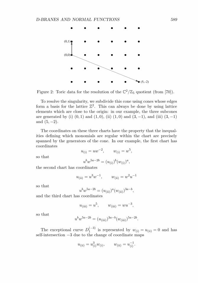
and note that the condition for this monomial to be regular, i.e., to haveno pole at the origin, b ≥ 0, 5a − 2b ≥ 0. These inequalities determine thetoric data: the dual vectors (0, 1) and (5,−2) generate a cone consisting ofall inequalities satisfied by regular monomials, as depicted in figure 2 (whichwas borrowed from [70]).
D-BRANES AND NORMAL FUNCTIONS 589
Figure 2: Toric data for the resolution of the C2/Z5 quotient (from [70]).
To resolve the singularity, we subdivide this cone using cones whose edgesform a basis for the lattice Z
2. This can always be done by using latticeelements which are close to the origin: in our example, the three subconesare generated by (i) (0, 1) and (1, 0), (ii) (1, 0) and (3,−1), and (iii) (3,−1)and (5,−2).
The coordinates on these three charts have the property that the inequal-ities defining which monomials are regular within the chart are preciselyspanned by the generators of the cone. In our example, the first chart hascoordinates
u(i) = uw−2, w(i) = w5,
so thatubw5a−2b = (u(i))
b(w(i))a,
the second chart has coordinates
u(ii) = u3w−1, w(ii) = w2u−1
so thatubw5a−2b = (u(ii))
a(w(ii))3a−b,
and the third chart has coordinates
u(iii) = u5, w(iii) = wu−3,
so thatubw5a−2b = (u(iii))
3a−b(w(iii))5a−2b.
The exceptional curve D(−3)1 is represented by w(i) = u(ii) = 0 and has
self-intersection −3 due to the change of coordinate maps
u(ii) = u3(i)w(i), w(ii) = u−1
(i) .

590 DAVID R. MORRISON AND JOHANNES WALCHER
The exceptional curve D(−2)1 is represented by w(ii) = u(iii) = 0 and has
self-intersection −2 due to the change of coordinate maps
u(iii) = u2(ii)w(ii), w(iii) = u−1
(ii).
The defining polynomial for the quintic mirror, when restricted to S, takesthe following form in these coordinate charts:
15w(i) − ψu2
(i)w(i) =15w(i)(1 −
√5ψu(i))(1 +
√5ψu(i)),
15u(ii)w
3(ii) − ψu(ii)w(ii) =
15u(ii)w(ii)(w(ii) −
√5ψ)(w(ii) +
√5ψ),
15u3
(iii)w5(iii) − ψu(iii)w(iii) =
15u(iii)w(iii)(u(iii)w
2(iii) −
√5ψ)(u(iii)w
2(iii) +
√5ψ).
Thus, the intersection points p1,± of C± with D(−3)1 can be found in either
chart (i) at (±(5ψ)−1/2, 0) or chart (ii) at (0,±(5ψ)1/2). All of these agreewith the illustration in figure 1.
We now turn to the resolution of the quintic mirror itself. In order todescribe the C
3/(Z5)2 quotient singularity in terms of toric geometry, werepresent an arbitrary invariant rational monomial in the form
(u5)a(v5)b(uvw)c = u5a+cv5b+cwc,
and note that the condition for this monomial to be regular is 5a + c ≥ 0,5b + c ≥ 0, and c ≥ 0. Those three inequalities determine the toric data:one takes the dual vectors (5, 0, 1), (0, 5, 1), (0, 0, 1) to these inequalities andnotes that all inequalities satisfied on the regular functions are non-negativelinear combinations of these vectors.
The resolutions of toric geometry are obtained by subdividing the conegenerated by those vectors into cones whose generating vectors give a basisfor the lattice Z
3. There are a number of ways of doing this, but we usethe symmetric one illustrated in figure 3 (which is borrowed from [71]). Thethree dual vectors (5, 0, 1), (0, 5, 1), (0, 0, 1) are the vertices of the largetriangle, and the resolution has coordinate charts determined by the smalltriangles in the diagram.
There are two kinds of coordinate charts. The first type of chart Uαβ ,labeled by α and β with α ≥ 0, β ≥ 0, and α + β ≤ 4, corresponds to theupward-pointing triangle in figure 3 with vertices (α, β + 1, 1), (α, β, 1), and

D-BRANES AND NORMAL FUNCTIONS 591
Figure 3: Toric data for the resolution of the C3/(Z5)2 quotient (from [71]).
(α + 1, β, 1). This chart will have coordinates Xαβ , Yαβ , Zαβ , and T = tsatisfying
(Xαβ)aα+b(β+1)+c(Yαβ)aα+bβ+c(Zαβ)a(α+1)+bβ+c = (u5)a(v5)b(uvw)c.
This can be solved for the coordinates, giving
T = t,
Xαβ = u−βv5−βw−β,
Yαβ = uα+β−4vα+β−4wα+β+1,
Zαβ = u5−αv−αw−α.
The defining polynomial of the quintic mirror in this chart is
15
(1 + T 5 + Xα
αβY ααβZα+1
αβ + Xβ+1αβ Y β
αβZβαβ + X4−α−β
αβ Y 5−α−βαβ Z4−α−β
αβ
)
− ψTXαβYαβZαβ .
The second type of chart Uαβ , labeled by α and β with α ≥ 0, β ≥ 0, andα + β ≤ 3, corresponds to the downward-pointing triangles in figure 3 withvertices (α, β + 1, 1), (α + 1, β + 1, 1), and (α + 1, β, 1). This chart will havecoordinates Xαβ , Yαβ , Zαβ , and T = t satisfying
(Xαβ)aα+b(β+1)+c(Yαβ)a(α+1)+b(β+1)+c(Zαβ)a(α+1)+bβ+c = (u5)a(v5)b(uvw)c.
This can be solved for the coordinates, giving
T = t,
Xαβ = uα−4vα+1wα+1,

592 DAVID R. MORRISON AND JOHANNES WALCHER
Yαβ = u4−α−βv4−α−βw−1−α−β ,
Zαβ = uβ+1vβ−4wβ+1.
The defining polynomial of the quintic mirror in this chart is
15
(1 + T 5 + Xα
αβY α+1αβ Zα+1
αβ + Xβ+1αβ Y β+1
αβ Zβαβ + X4−α−β
αβ Y 3−α−βαβ Z4−α−β
αβ
)
− ψT XαβYαβZαβ .
To determine which chart we should use, we restrict the coordinates onUαβ and Uαβ to the blowup of S and express them as functions of thecoordinates u(i) and w(i) in the first coordinate chart of that blowup. InUαβ we find
T = 1,
Xαβ = (−1)5−βu5−2β(i) w2−β
(i) ,
Yαβ = (−1)α+β−4u2α+2β−8(i) wα+β−3
(i) ,
Zαβ = (−1)αu5−2α(i) w2−α
(i) ,
and from this we conclude that U22 restricts to this coordinate chart on S,and contains the points p1,±. In Uαβ we find
T = 1,
Xαβ = (−1)α+1u2α−3(i) wα−1
(i) ,
Yαβ = (−1)4−α−βu8−2α−2β(i) w3−α−β
(i) ,
Zαβ = (−1)β−4u2β−3(i) wβ−1
(i) ,
and so none of the coordinate charts Uαβ is a neighborhood of p1,±.
Thus, the first coordinate chart we use will have coordinates
T = T22 = t = x−11 x2,
X = X22 = u−2v3w−2 = x1x−23 x3
4x−25 ,
Y = Y22 = w5 = x−51 x5
5,
Z = Z22 = u3v−2w−2 = x1x33x
−24 x−2
5 ,

D-BRANES AND NORMAL FUNCTIONS 593
and polynomial
15
(1 + T 5 + X2Y 2Z3 + X3Y 2Z2 + Y
)− ψTXY Z.
The resolution S of the surface S is given by T = −1 and Z = −X, and therestriction of the polynomial to S is
15Y − ψX2Y =
15Y (1 +
√5ψX)(1 −
√5ψX).
The points p1,± are given by X = ±1/√
5ψ and Y = 0.
To find a neighborhood of the points p2,±, we use the affine chart x3 = 1and label the coordinates on this chart as u′ = x1/x3, v′ = x2/x3, t′ = x4/x3,and w′ = x5/x3. The defining polynomial becomes
15
((u′)5 + (v′)5 + 1 + (t′)5 + (w′)5
)− ψt′u′v′w′,
and the surface S is defined by t′ = −1 and v′ = −u′. We have chosen thenotation so that the (Z5)2 subgroup of (Z5)3 which stabilizes p2 acts exactlyas in the previous case: acting on (u′, v′, w′) and preserving the productu′v′w′.
Since the combinatorics are identical, the computation produces the sameresult as in the first part of this appendix. We find a neighborhood of p2,±with coordinates
T ′ = t′ = x−13 x4,
X ′ = (u′)−2(v′)3(w′)−2 = x−21 x3
2x3x−25 ,
Y ′ = (w′)5 = x−53 x5
5,
Z ′ = (u′)3(v′)−2(w′)−2 = x31x
−22 x3x
−25 ,
and polynomial
15
((X ′)2(Y ′)2(Z ′)3 + (X ′)3(Y ′)2(Z ′)21 + (T ′)5 + +Y ′) − ψTXY Z.
The resolution S of the surface S is given by T ′ = −1 and Z ′ = −X ′, andthe restriction of the polynomial to S is
15Y ′ − ψ(X ′)2Y ′ =
15Y ′(1 +
√5ψX ′)(1 −
√5ψX ′).
The points p2,± are given by X ′ = ±1/√
5ψ and Y ′ = 0.

594 DAVID R. MORRISON AND JOHANNES WALCHER
Just for completeness, we include the change of coordinates between thesetwo charts.
T ′ = 5
√X
Z,
X ′ = T 3 5√
X2Z3,
Y ′ =1
(X2Y Z3),
Z ′ = T−2 5√
X2Z3.
These formulas illustrate the important point that the additional Z5 quotientmust be considered in each case.
References
[1] P. Candelas, M. Lynker and R. Schimmrigk, Calabi–Yau manifolds inweighted P4, Nucl. Phys. B 341 (1990), 383–402.
[2] B.R. Greene and M.R. Plesser, Duality in Calabi–Yau moduli space,Nucl. Phys. B 338 (1990), 15–37.
[3] P.S. Aspinwall, C.A. Lutken and G.G. Ross, Construction and couplingsof mirror manifolds, Phys. Lett. B 241 (1990), 373–380.
[4] P. Candelas, X.C. De La Ossa, P.S. Green and L. Parkes, A pairof Calabi–Yau manifolds as an exactly soluble superconformal theory,Nucl. Phys. B 359 (1991), 21–74.
[5] D.R. Morrison, Mirror symmetry and rational curves on quintic three-folds: a guide for mathematicians, J. Am. Math. Soc. 6 (1993), 223–247,arXiv:alg-geom/9202004.
[6] A.B. Givental, Equivariant Gromov–Witten invariants, Int. Math. Res.Not. 13 (1996), 613–663, arXiv:alg-geom/9603021.
[7] B.H. Lian, K. Liu and S.-T. Yau, Mirror principle I, Asian J. Math. 1(1997), 729–763, arXiv:alg-geom/9712011.
[8] D.R. Morrison and M.R. Plesser, Towards mirror symmetry as dualityfor two-dimensional abelian gauge theories, Nucl. Phys. Proc. Suppl.46 (1996), 177–186, arXiv:hep-th/9508107.
[9] K. Hori and C. Vafa, Mirror symmetry, arXiv:hep-th/0002222.[10] E. Witten, Chern–Simons gauge theory as a string theory, Prog. Math.
133 (1995), 637–678, arXiv:hep-th/9207094.[11] M. Kontsevich, Homological algebra of mirror symmetry, Proc. Int.
Congr. Math., Zurich, 1994, Vol. 1, Birkhauser, 1995, pp. 120–139,arXiv:alg-geom/9411018.
D-BRANES AND NORMAL FUNCTIONS 595
[12] A. Strominger, S.-T. Yau and E. Zaslow, Mirror symmetry is T-duality,Nucl. Phys. B 479 (1996), 243–259, arXiv:hep-th/9606040.
[13] R. Gopakumar and C. Vafa, M-theory and topological strings I and II,arXiv:hep-th/9809187, arXiv:hep-th/9812127.
[14] M.R. Douglas, D-branes, categories and N = 1 supersymmetry, J. Math.Phys. 42 (2001), 2818–2843, arXiv:hep-th/0011017.
[15] P.S. Aspinwall and A.E. Lawrence, Derived categories and zero-branestability, JHEP 08 (2001), 004, arXiv:hep-th/0104147.
[16] A. Kapustin and L. Rozansky, On the relation between open andclosed topological strings, Commun. Math. Phys. 252 (2004), 393–414,arXiv:hep-th/0405232.
[17] K. Costello, Topological conformal field theories and Calabi–Yau cate-gories, Adv. Math. 210 (2007), 165–214, arXiv:math.QA/0412149.
[18] A. Caldararu and S. Willerton, The Mukai pairing I, A categoricalapproach, arXiv:0707.2052 [math.AG].
[19] J. Walcher, Opening mirror symmetry on the quintic, Commun. Math.Phys., 276 (2007), 671–689 arXiv:hep-th/0605162.
[20] G. Almkvist, private communication.[21] V. Shende, private communication.[22] R. Pandharipande, J. Solomon and J. Walcher, Disk enumeration on
the quintic 3-fold, arXiv:math.SG/0610901.[23] M. Aganagic and C. Vafa, Mirror symmetry, D-branes and counting
holomorphic discs, arXiv:hep-th/0012041.[24] M. Aganagic, A. Klemm and C. Vafa, Disk instantons, mirror sym-
metry and the duality web, Z. Naturforsch. A 57 (2002), 1–28,arXiv:hep-th/0105045.
[25] T. Graber and E. Zaslow, Open-string Gromov–Witten invariants:calculations and a mirror “theorem”, Orbifolds in mathematics andphysics, Contemp. Math., Vol. 310, American Mathematical Society,2002, pp. 107–121, arXiv:hep-th/0109075.
[26] P. Mayr, Summing up open string instantons and N = 1 string ampli-tudes, arXiv:hep-th/0203237.
[27] W. Lerche, P. Mayr and N. Warner, Holomorphic N = 1 special geom-etry of open–closed type II strings, arXiv:hep-th/0207259.
[28] , N = 1 special geometry, mixed Hodge variations and toricgeometry, arXiv:hep-th/0208039.
[29] S. Govindarajan, T. Jayaraman and T. Sarkar, Disc instantonsin linear sigma models, Nucl. Phys. B 646 (2002), 498–523,arXiv:hep-th/0108234.

596 DAVID R. MORRISON AND JOHANNES WALCHER
[30] B. Forbes, Open string mirror maps from Picard–Fuchs equations, Mir-ror symmetry, V, AMS/IP Stud. Adv. Math., Vol. 38, American Math-ematical Society, 2006, pp. 561–570, arXiv:hep-th/0307167.
[31] E. Witten, Branes and the dynamics of QCD, Nucl. Phys. B 507 (1997),658–690, arXiv:hep-th/9706109.
[32] P.A. Griffiths, A theorem concerning the differential equations satisfiedby normal functions associated to algebraic cycles, Am. J. Math. 101(1979), 94–131.
[33] P.L. del Angel and S. Muller-Stach, Differential systems associated tofamilies of algebraic cycles, arXiv:math.AG/0305288.
[34] J. Walcher, Extended holomorphic anomaly and loop amplitudes in opentopological string, arXiv:hep-th/0705.4098.
[35] P.A. Griffiths, On the periods of certain rational integrals I and II, Ann.Math. 90 (2), (1969), 460–495; ibid. 90 (2), (1969), 496–541.
[36] C.I. Lazaroiu, String field theory and brane superpotentials, JHEP 10(2001), 018, arXiv:hep-th/0107162.
[37] A. Tomasiello, A-infinity structure and superpotentials, JHEP 09(2001), 030, arXiv:hep-th/0107195.
[38] M.L. Green, Infinitesimal methods in Hodge theory, Algebraic cyclesand Hodge theory, Lecture Notes in Mathematics, Vol. 1594, Springer,1994, pp. 1–92.
[39] C. Voisin, Hodge theory and complex algebraic geometry II, Cam-bridge Studies in Advanced Mathematics, Vol. 77, Cambridge Univer-sity Press, 2003.
[40] ———, Hodge theory and complex algebraic geometry I, CambridgeStudies in Advanced Mathematics, Vol. 76, Cambridge UniversityPress, 2002.
[41] H. Clemens, Homological equivalence, modulo algebraic equivalence, isnot finitely generated, Publ. Math. IHES 58 (1983), 19–38.
[42] C. Voisin, The Griffiths group of a general Calabi–Yau threefold is notfinitely generated, Duke Math. J. 102 (2000), 151–186.
[43] E. Witten, New issues in manifolds of SU(3) holonomy, Nucl. Phys. B268 (1986), 79–112.
[44] C.I. Lazaroiu, D-brane categories, Int. J. Mod. Phys. A 18 (2003), 5299–5335, arXiv:hep-th/0305095.
[45] S.K. Donaldson and R.P. Thomas, Gauge theory in higher dimensions,The geometric universe, Oxford University Press, 1998, pp. 31–47.
[46] H. Clemens, Cohomology and Obstructions II: Curves on K-trivialThreefolds, arXiv:math.AG/0206219.

D-BRANES AND NORMAL FUNCTIONS 597
[47] A.N. Tyurin, Nonabelian analogues of Abel’s theorem, Izv. Ross.Akad. Nauk Ser. Mat. 65 (2001), 133–196; Izvestija Math. 65 (2001),123–180.
[48] C. Vafa, Extending mirror conjecture to Calabi–Yau with bundles,arXiv:hep-th/9804131.
[49] S. Kachru, S. Katz, A.E. Lawrence and J. McGreevy, Open stringinstantons and superpotentials, Phys. Rev. D 62 (2000), 026001,arXiv:hep-th/9912151.
[50] R. Dijkgraaf and C. Vafa, Matrix models, topological strings, andsupersymmetric gauge theories, Nucl. Phys. B 644 (2002), 3–20,arXiv:hep-th/0206255.
[51] A. Grothendieck, La theorie des classes de Chern, Bull. Soc. Math.France 86 (1958), 137–154.
[52] P. Deligne, Local behavior of Hodge structures at infinity, Mirror sym-metry, II, AMS/IP Stud. Adv. Math., Vol. 1, American MathematicalSociety, 1997, pp. 683–699.
[53] D.R. Morrison, Compactifications of moduli spaces inspired by mir-ror symmetry, Journees de Geometrie Algebrique d’Orsay, Asterisque,Vol. 218, Societe Mathematique de France, 1993, pp. 243–271,arXiv:alg-geom/9304007.
[54] ———, Mathematical aspects of mirror symmetry, Complex AlgebraicGeometry, J. Kollar, ed., IAS/Park City Math. Series, Vol. 3, 1997, pp.265–340, arXiv:alg-geom/9609021.
[55] K. Fukaya, Y.-G. Oh, H. Ohto and K. Ono, Lagrangian intersectiontheory — anomaly and obstruction, Kyoto University preprint, 2000.
[56] J.P. Solomon, Intersection theory on the moduli space of holomorphiccurves with Lagrangian boundary conditions, arXiv:math.SG/0606429.
[57] J. Walcher, Stability of Landau–Ginzburg branes, J. Math. Phys. 46(2005), 082305, arXiv:hep-th/0412274.
[58] D. Orlov, Derived categories of coherent sheaves and triangulated cate-gories of singularities, arXiv:math.AG/0503632.
[59] P.S. Aspinwall, The Landau–Ginzburg to Calabi–Yau dictionary forD-branes, arXiv:hep-th/0610209.
[60] M. Herbst, K. Hori and D. Page, Phases of N = 2 theories in 1 + 1dimensions with boundary, arXiv:hep-th/0803-2045; talks at MSRIBerkeley (March 2006), LMU Munich (July 2006), IAS Princeton (Jan-uary 2007).
[61] I. Brunner, M.R. Douglas, A.E. Lawrence and C. Romelsberger,D-branes on the quintic, JHEP 08 (2000), 015, arXiv:hep-th/9906200.
598 DAVID R. MORRISON AND JOHANNES WALCHER
[62] A. Recknagel and V. Schomerus, D-branes in Gepner models, Nucl.Phys. B 531 (1998), 185–225, arXiv:hep-th/9712186.
[63] K. Hori, A. Iqbal and C. Vafa, D-branes and mirror symmetry,arXiv:hep-th/0005247.
[64] K. Hori, Boundary RG flows of N = 2 minimal models, Mirror sym-metry, V, AMS/IP Stud. Adv. Math., Vol. 38, American MathematicalSociety, 2006, pp. 381–404, arXiv:hep-th/0401139.
[65] K. Hori and J. Walcher, D-branes from matrix factorizations, ComptesRendus Physique 5 (2004), 1061–1070, arXiv:hep-th/0409204.
[66] E. Witten, Phases of N = 2 theories in two dimensions, Nucl. Phys. B403 (1993) 159–222, arXiv:hep-th/9301042.
[67] I. Brunner, K. Hori, K. Hosomichi and J. Walcher, Orientifolds of Gep-ner models, JHEP 02 (2007), 001, arXiv:hep-th/0401137.
[68] F. Hirzebruch, Uber vierdimensionale Riemannsche Flachenmehrdeutiger analytischer Funktionen von zwei komplexenVeranderlichen, Math. Ann. 126 (1953), 1–22.
[69] H.W.E. Jung, Darstellung der Funktionen eines algebraischen Korperszweier unabhangiger Veranderlicher x, y in der Umgebung einer Stellex = a, y = b, J. Reine Angew. Math. 133 (1908), 289–314.
[70] J.A. Harvey, D. Kutasov, E.J. Martinec and G.W. Moore, Localizedtachyons and RG flows, arXiv:hep-th/0111154.
[71] D.R. Morrison, Geometric aspects of mirror symmetry, Mathemat-ics unlimited — 2001 and beyond, Springer, 2001, pp. 899–918,arXiv:math.AG/0007090.