Embed Size (px)
Citation preview
1
Cyber Physical Power Systems
Week #1
© A. Kwasinski, 2015
2Cyber-physical systems
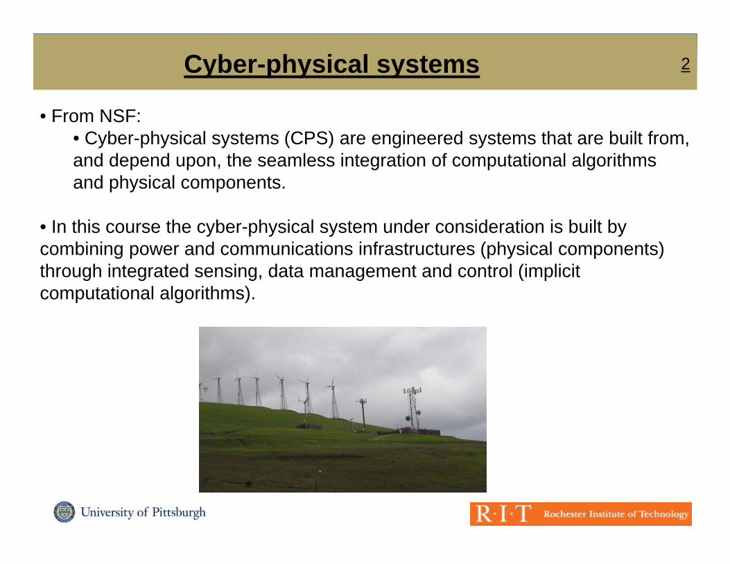
• From NSF:• Cyber-physical systems (CPS) are engineered systems that are built from, and depend upon, the seamless integration of computational algorithms
d h i land physical components.
• In this course the cyber-physical system under consideration is built by combining power and communications infrastructures (physical components)combining power and communications infrastructures (physical components) through integrated sensing, data management and control (implicit computational algorithms).
© A. Kwasinski, 2015
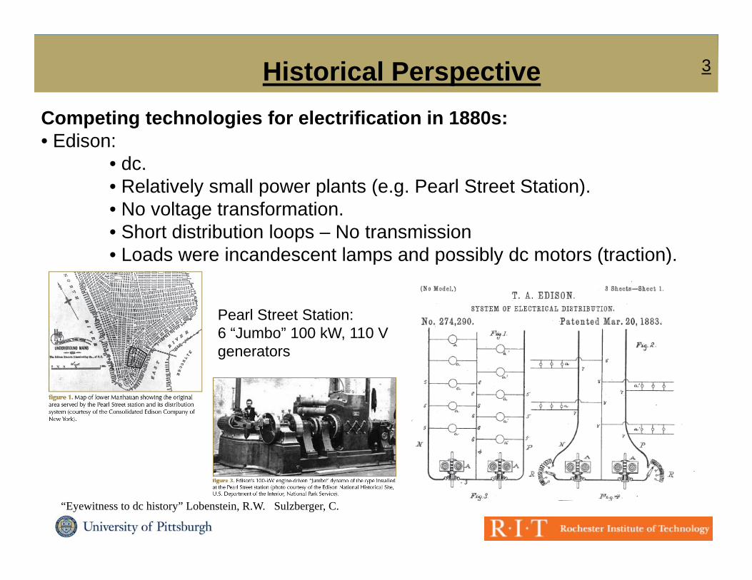
3Historical PerspectiveCompeting technologies for electrification in 1880s: • Edison:
• dc.R l ti l ll l t ( P l St t St ti )• Relatively small power plants (e.g. Pearl Street Station).
• No voltage transformation.• Short distribution loops – No transmission• Loads were incandescent lamps and possibly dc motors (traction)• Loads were incandescent lamps and possibly dc motors (traction).
Pearl Street Station:6 “Jumbo” 100 kW, 110 Vgenerators
© A. Kwasinski, 2015
“Eyewitness to dc history” Lobenstein, R.W. Sulzberger, C.
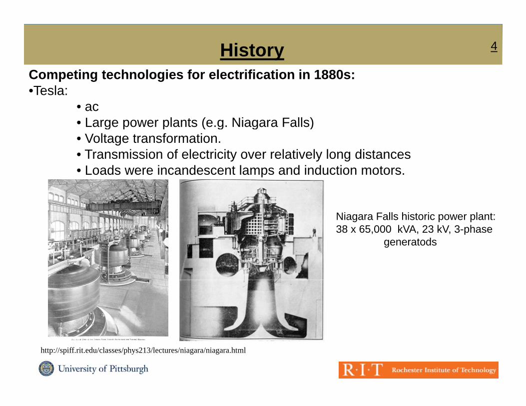
4HistoryCompeting technologies for electrification in 1880s:Competing technologies for electrification in 1880s: •Tesla:
• ac• Large power plants (e.g. Niagara Falls)Large power plants (e.g. Niagara Falls)• Voltage transformation.• Transmission of electricity over relatively long distances• Loads were incandescent lamps and induction motors.
Niagara Falls historic power plant:38 x 65 000 kVA 23 kV 3 phase38 x 65,000 kVA, 23 kV, 3-phase
generatods
© A. Kwasinski, 2015
http://spiff.rit.edu/classes/phys213/lectures/niagara/niagara.html

5Power Grids Topology
• Divided among the following partsGeneration
Transmission
Distribution / consumption
Generation
GenerationGeneration
Distribution /
© A. Kwasinski, 2015
Distribution / consumption
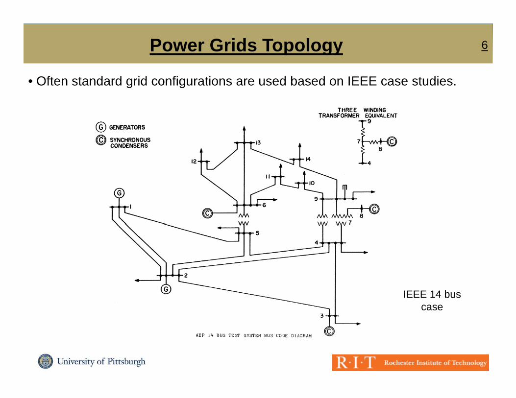
6Power Grids Topology
• Often standard grid configurations are used based on IEEE case studies.
IEEE 14 bus case
© A. Kwasinski, 2015

7Generation
• Electric power is generated at power stations.
• Generated power = load + losses
• Electric power generators are classified between base and peaking units.
Wind + PV
Peaking units
Natural gas, liquid fuelsHydroelectric
Base units Coal
Nuclear
© A. Kwasinski, 2015

8Generation
P ki it• Peaking units:• The tend to be used to follow the load. • Most of them are fueled by natural gas but some units using liquid fuels are also usedare also used.• They tend to have a relatively faster response (their power output can be adjusted relatively fast) and they tend to come online and offline relatively oftenoften.• Their power output is in the range of a few 100s MW to a very few 1000s MW.
© A. Kwasinski, 2015
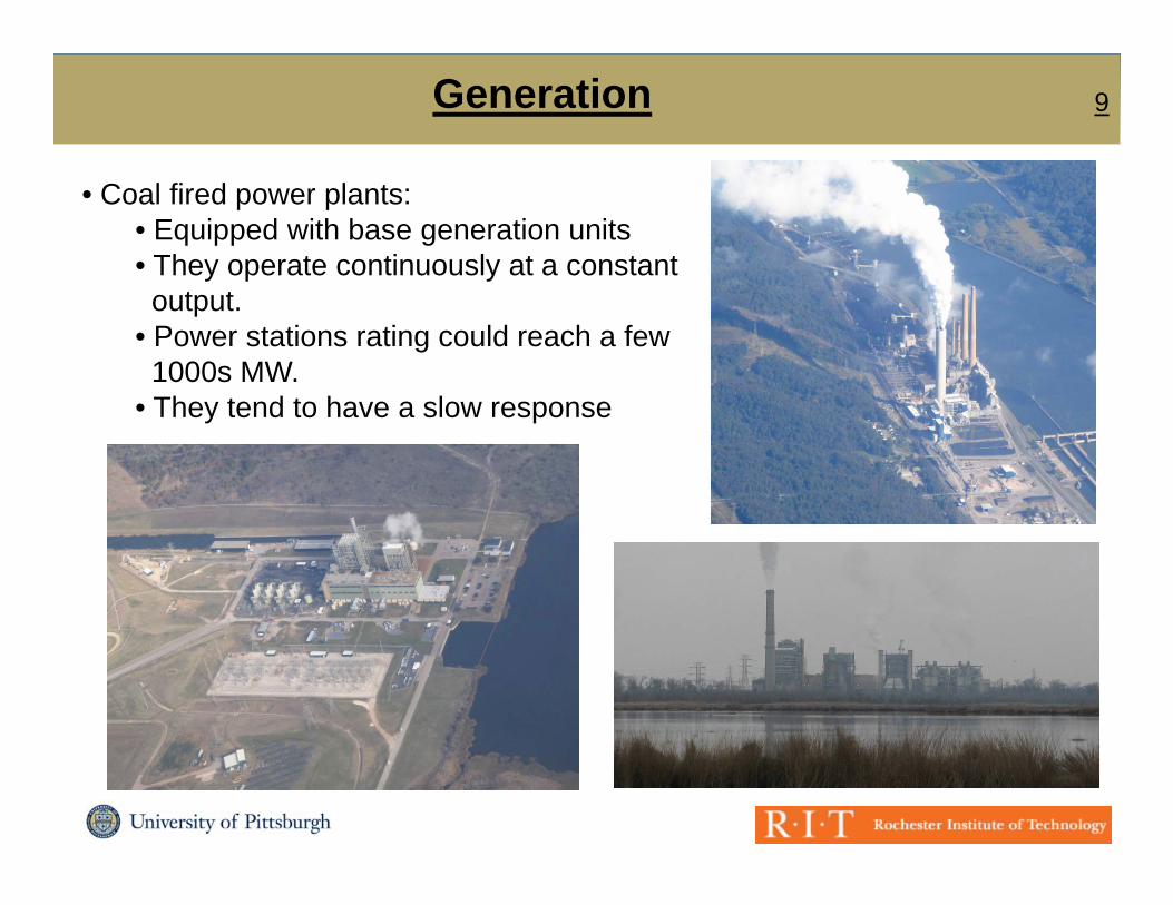
9Generation
• Coal fired power plants:• Equipped with base generation units• They operate continuously at a constantoutput.
• Power stations rating could reach a few1000s MW.
• They tend to have a slow response
© A. Kwasinski, 2015
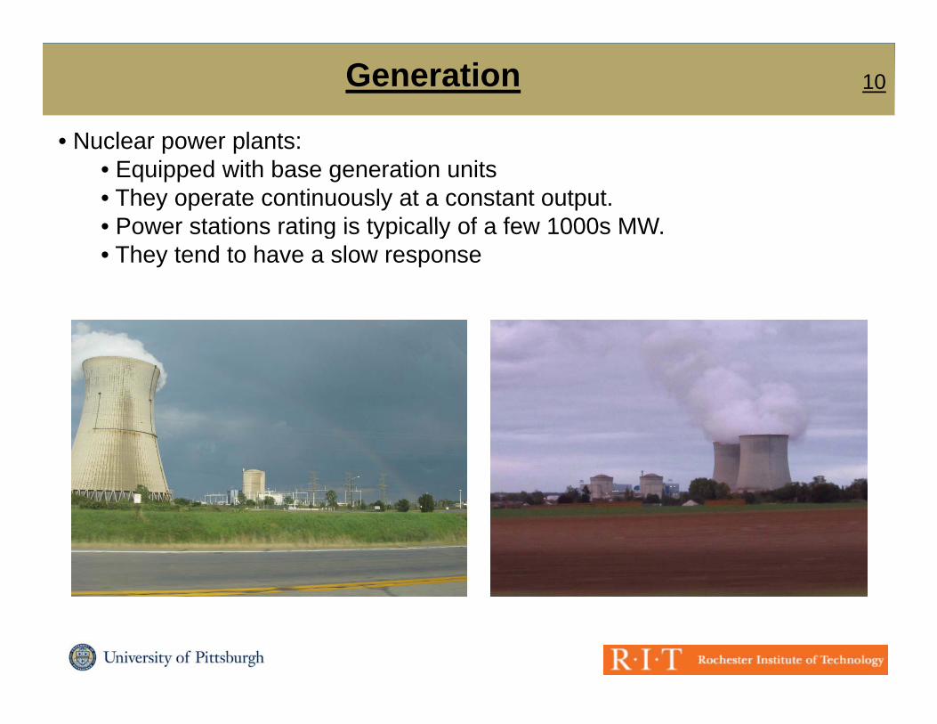
10Generation
N l l t• Nuclear power plants:• Equipped with base generation units• They operate continuously at a constant output.• Power stations rating is typically of a few 1000s MW• Power stations rating is typically of a few 1000s MW.• They tend to have a slow response
© A. Kwasinski, 2015
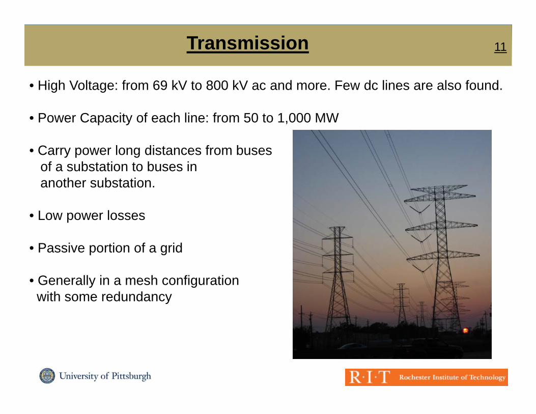
11Transmission
• High Voltage: from 69 kV to 800 kV ac and more. Few dc lines are also found.
• Power Capacity of each line: from 50 to 1,000 MW
• Carry power long distances from busesof a substation to buses in another substationanother substation.
• Low power losses
• Passive portion of a grid
• Generally in a mesh configurationy gwith some redundancy
© A. Kwasinski, 2015
12Distribution
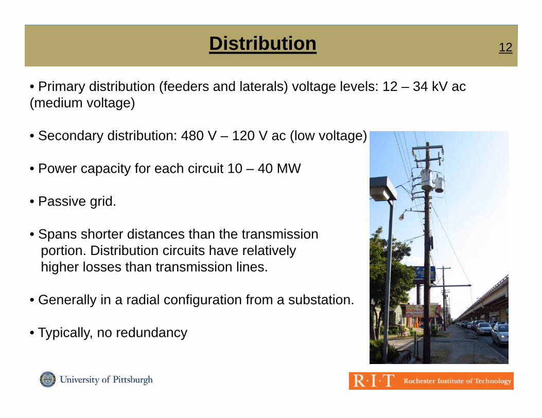
• Primary distribution (feeders and laterals) voltage levels: 12 – 34 kV ac (medium voltage)
• Secondary distribution: 480 V – 120 V ac (low voltage)
• Power capacity for each circuit 10 – 40 MW
• Passive grid.
• Spans shorter distances than the transmission• Spans shorter distances than the transmissionportion. Distribution circuits have relativelyhigher losses than transmission lines.
• Generally in a radial configuration from a substation.
• Typically, no redundancy
© A. Kwasinski, 2015
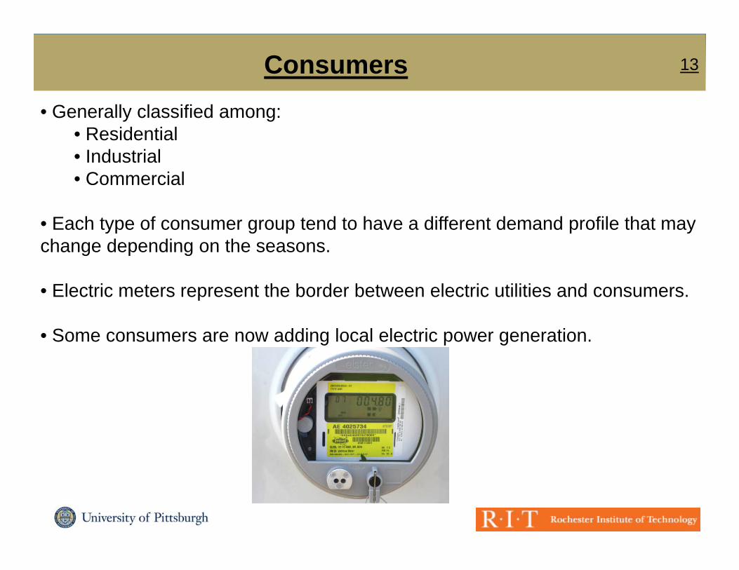
13ConsumersG ll l ifi d• Generally classified among:
• Residential• Industrial• Commercial• Commercial
• Each type of consumer group tend to have a different demand profile that may change depending on the seasonschange depending on the seasons.
• Electric meters represent the border between electric utilities and consumers.
• Some consumers are now adding local electric power generation.
© A. Kwasinski, 2015
14Substations
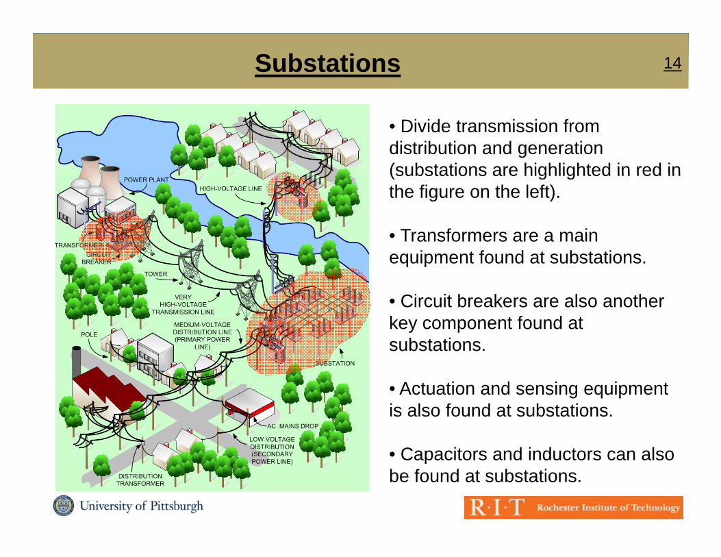
• Divide transmission from distribution and generation (substations are highlighted in red in(substations are highlighted in red in the figure on the left).
• Transformers are a main equipment found at substations.
• Circuit breakers are also another key component found at substations.
A t ti d i i t• Actuation and sensing equipment is also found at substations.
• Capacitors and inductors can also
© A. Kwasinski, 2015
• Capacitors and inductors can also be found at substations.

15
L t l
SubstationsLayout examples:
© A. Kwasinski, 2015
16
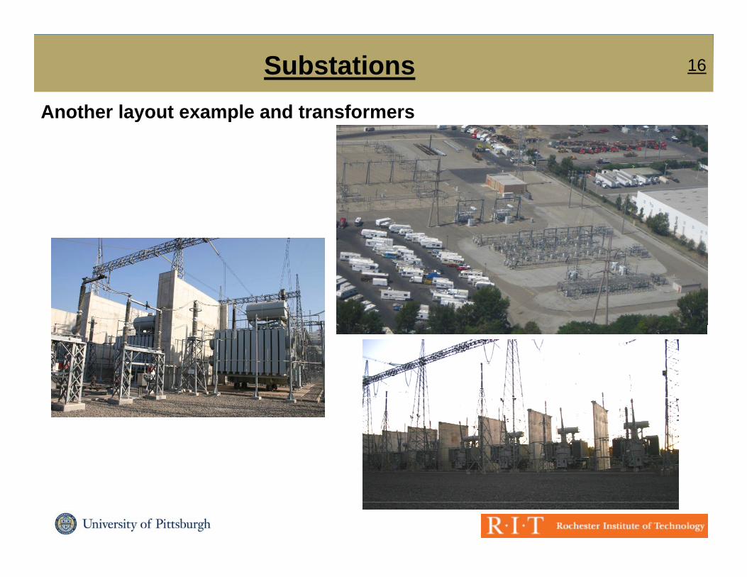
A th l t l d t f
SubstationsAnother layout example and transformers
© A. Kwasinski, 2015
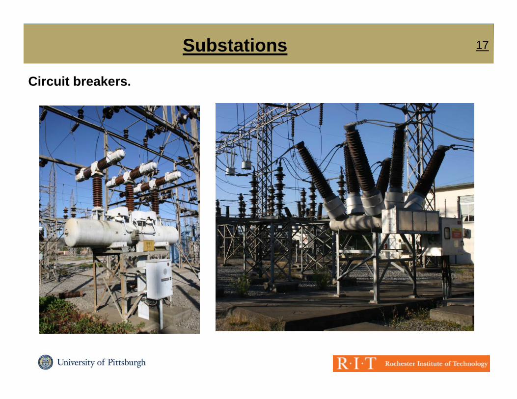
17Substations
Circuit breakers.
© A. Kwasinski, 2015

18Substations
Sensing and actuation components (a lot more about this throughout this course).
© A. Kwasinski, 2015
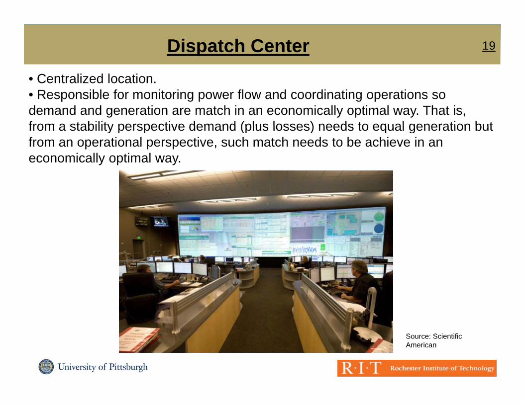
19Dispatch CenterC t li d l ti• Centralized location.
• Responsible for monitoring power flow and coordinating operations so demand and generation are match in an economically optimal way. That is, from a stability perspective demand (plus losses) needs to equal generation butfrom a stability perspective demand (plus losses) needs to equal generation but from an operational perspective, such match needs to be achieve in an economically optimal way.
© A. Kwasinski, 2015
Source: Scientific American
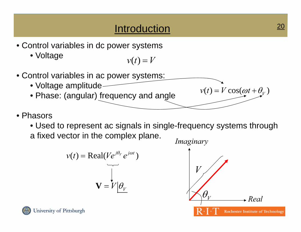
20IntroductionC t l i bl i d t• Control variables in dc power systems
• Voltage
C
Vtv )(• Control variables in ac power systems:
• Voltage amplitude• Phase: (angular) frequency and angle ( ) cos( )Vv t V t
• Phasors• Used to represent ac signals in single-frequency systems through a fixed vector in the complex plane.
( ) Real( )Vj j tv t Ve e
Imaginary
( ) ( )
VV V
V
© A. Kwasinski, 2015
V
V Real
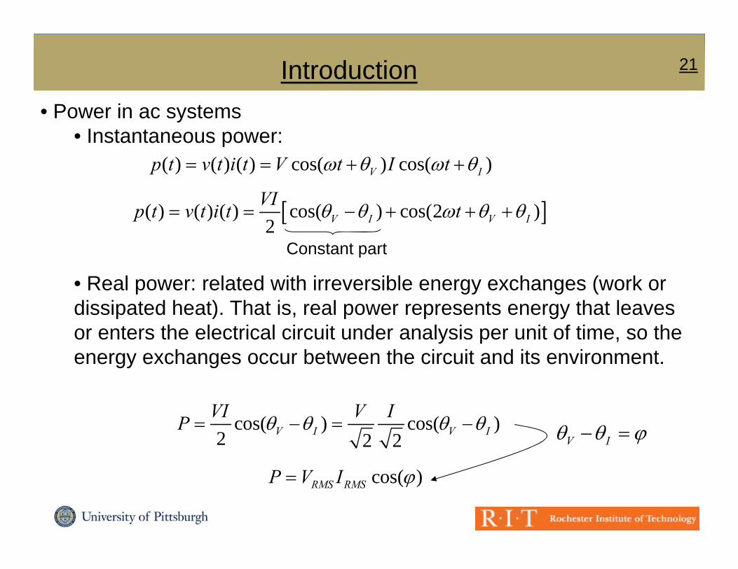
21IntroductionP i t• Power in ac systems
• Instantaneous power:( ) ( ) ( ) cos( ) cos( )V Ip t v t i t V t I t
( ) ( ) ( ) cos( ) cos(2 )2 V I V I
VIp t v t i t t
Constant part
• Real power: related with irreversible energy exchanges (work or dissipated heat). That is, real power represents energy that leaves
Constant part
or enters the electrical circuit under analysis per unit of time, so the energy exchanges occur between the circuit and its environment.
cos( ) cos( )2 2 2V I V I
VI V IP V I
© A. Kwasinski, 2015
cos( )RMS RMSP V I

22IntroductionP i t• Power in ac systems
• Complex power• Notice that
1 1 11 1 11 1 11 1 11 1 1
and that
*1 1 1Real( ) Real Real2 2 2V IP VI VI VI *1 1 1Real( ) Real Real2 2 2V IP VI VI VI *1 1 1Real( ) Real Real2 2 2V IP VI VI VI *1 1 1Real( ) Real Real2 2 2V IP VI VI VI *1 1 1Real( ) Real Real2 2 2V IP VI VI VI
• So a magnitude called complex power S is defined as
*1 1 1Imaginary( ) Imaginary Imaginary2 2 2V IQ VI VI VI *1 1 1Imaginary( ) Imaginary Imaginary2 2 2V IQ VI VI VI *1 1 1Imaginary( ) Imaginary Imaginary2 2 2V IQ VI VI VI *1 1 1Imaginary( ) Imaginary Imaginary2 2 2V IQ VI VI VI *1 1 1Imaginary( ) Imaginary Imaginary2 2 2V IQ VI VI VI
So a magnitude called complex power S is defined as
2 ( )I R jX SQ = 0 (resistive load)
Q > 0 (inductive load)* (cos sin )RMS RMSV I j S VI* (cos sin )RMS RMSV I j S VI2 ( )I R jX S
* (cos sin )RMS RMSV I j S VI2 ( )I R jX S
* (cos sin )RMS RMSV I j S VI
• Power factor (in power systems with one frequency) is defined as
( )RMSI R jX S
P P • It provides an idea of how efficient is the
Q < 0 (capacitive load)( )RMSI R jX S ( )RMSI R jX S
© A. Kwasinski, 2015
2 2. . cos P Pp f
S P Q
• It provides an idea of how efficient is the process of using (and generating) electrical power in ac circuits:
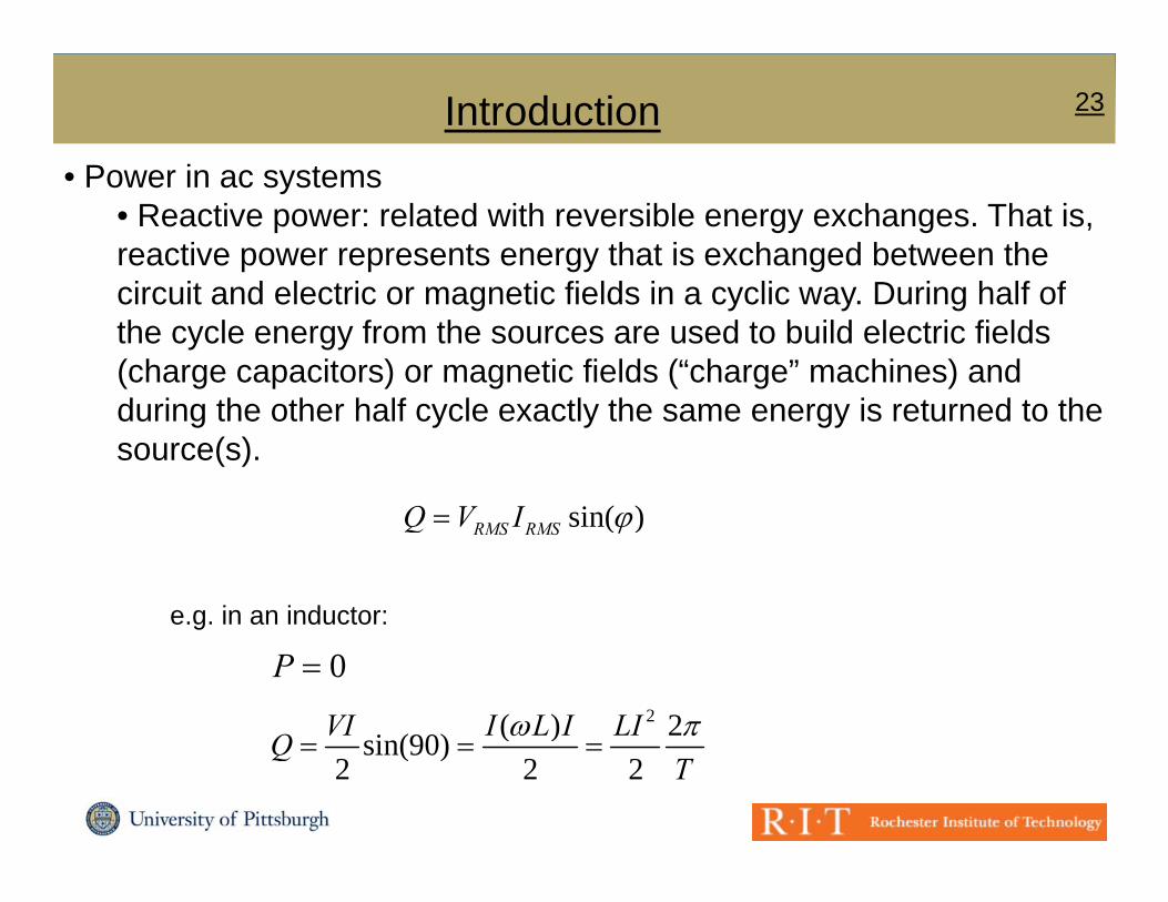
23IntroductionP i t• Power in ac systems
• Reactive power: related with reversible energy exchanges. That is, reactive power represents energy that is exchanged between the
f f fcircuit and electric or magnetic fields in a cyclic way. During half of the cycle energy from the sources are used to build electric fields (charge capacitors) or magnetic fields (“charge” machines) and during the other half cycle exactly the same energy is returned to the source(s).
i ( )Q V I
e.g. in an inductor:
sin( )RMS RMSQ V I
0P
e.g. in an inductor:
2( ) 2i (90)VI I L I LIQ
© A. Kwasinski, 2015
( )sin(90)2 2 2
VQT
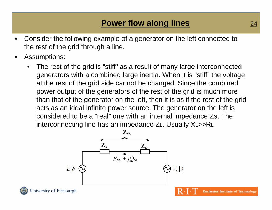
24Power flow along lines
• Consider the following example of a generator on the left connected to• Consider the following example of a generator on the left connected to the rest of the grid through a line.
• Assumptions: The rest of the grid is “stiff” as a res lt of man large interconnected• The rest of the grid is “stiff” as a result of many large interconnected generators with a combined large inertia. When it is “stiff” the voltage at the rest of the grid side cannot be changed. Since the combined power output of the generators of the rest of the grid is much morepower output of the generators of the rest of the grid is much more than that of the generator on the left, then it is as if the rest of the grid acts as an ideal infinite power source. The generator on the left is considered to be a “real” one with an internal impedance Zs. Theconsidered to be a real one with an internal impedance Zs. The interconnecting line has an impedance ZL. Usually XL>>RL
© A. Kwasinski, 2015
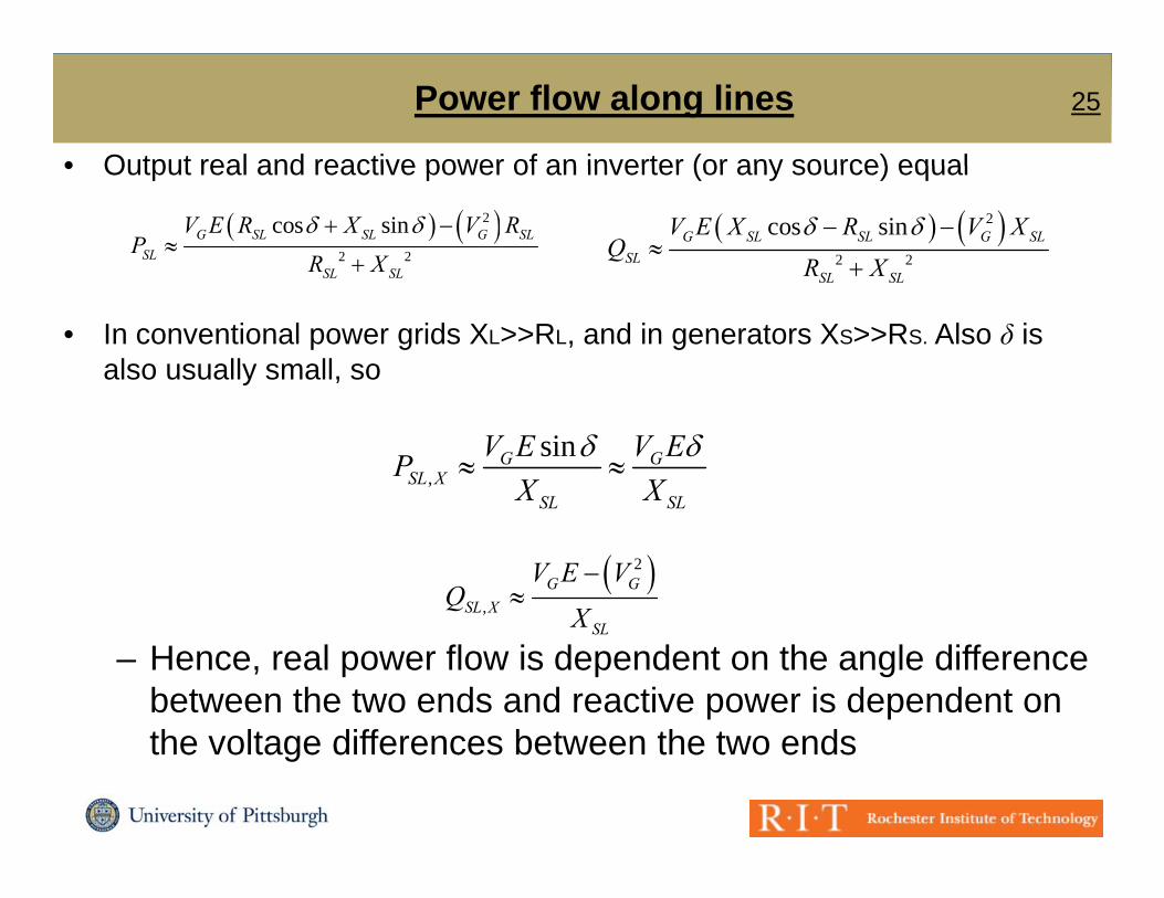
25Power flow along lines
• Output real and reactive power of an inverter (or any source) equal• Output real and reactive power of an inverter (or any source) equal
2
2 2
cos sinG SL SL G SLSL
SL SL
V E R X V RP
R X
2
2 2
cos sinG SL SL G SLSL
SL SL
V E X R V XQ
R X
• In conventional power grids XL>>RL, and in generators XS>>RS. Also δ is also usually small, so
SL SL
,sinG G
SL XSL SL
V E V EPX X
SL SL
2
,G G
SL X
V E VQ
X
– Hence, real power flow is dependent on the angle difference between the two ends and reactive power is dependent on th lt diff b t th t d
SLX
© A. Kwasinski, 2015
the voltage differences between the two ends
26
C id th f ll i l f ll 4 b id
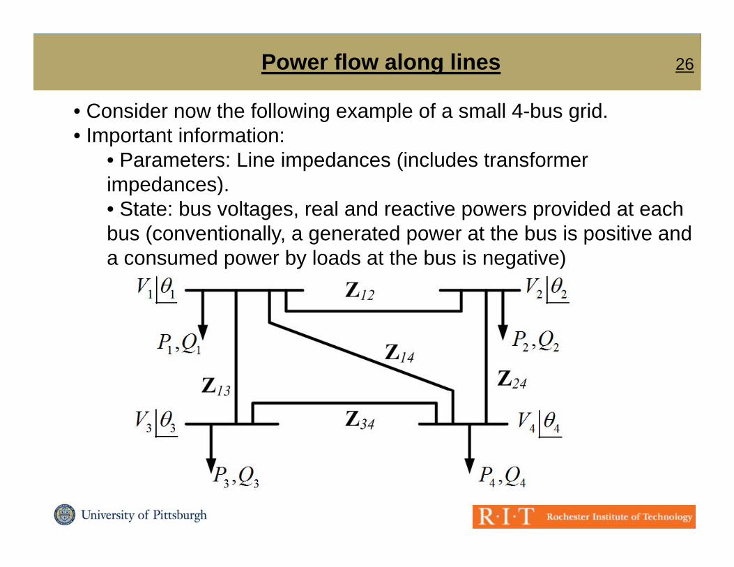
Power flow along lines
• Consider now the following example of a small 4-bus grid.• Important information:
• Parameters: Line impedances (includes transformer )impedances).
• State: bus voltages, real and reactive powers provided at each bus (conventionally, a generated power at the bus is positive and a consumed power by loads at the bus is negative)
© A. Kwasinski, 2015
27
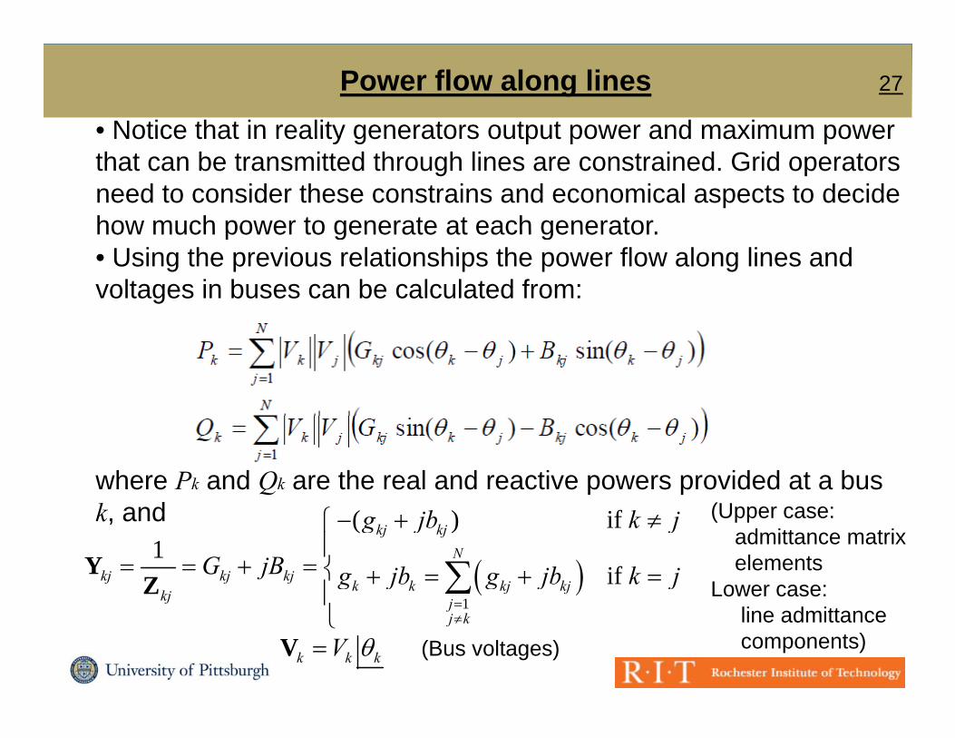
• Notice that in reality generators output power and maximum power
Power flow along linesNotice that in reality generators output power and maximum power
that can be transmitted through lines are constrained. Grid operators need to consider these constrains and economical aspects to decide how much power to generate at each generatorhow much power to generate at each generator.• Using the previous relationships the power flow along lines and voltages in buses can be calculated from:
where Pk and Qk are the real and reactive powers provided at a bus k and (Upper case:k, and
1
( ) if 1
if
kj kjN
kj kj kjk k kj kj
kj j
g jb k j
G jB g jb g jb k j
Y
Z
(Upper case:admittance matrix elements
Lower case:
© A. Kwasinski, 2015
1j jj k
line admittance
components)(Bus voltages)k k kV V

28
C id i i X/R ti h hi h th 1 ll l
Power flow along lines
• Considering once again X/R ratios much higher than 1, small angle differences, and per unit relative voltage magnitudes at each bus close to 1, the previous equations can be simplified to the dc power fflow equations
1 1
( ) ( )N N
k k j kj k j kj k jj j
P V V B B 1 1j j
j k j k
2 2
1 1
N N
k k k k kj k j k kj k jj j
Q V b V b V V V b V V
• Then, the power flow along lines is given by
j jj k j k
( )P B ( )kj kj k jP B
k kj k k jQ b V V V
© A. Kwasinski, 2015

29
• To find the power flow along lines we need to calculate:
Power flow along lines
• To find the power flow along lines we need to calculate:
• To calculate the above equation we need to solve
( )kj kj k jP B
• To calculate the above equation we need to solve
1
( )N
k kj k jj
P B
• This is an undetermined system of equations (the matrix is singular) then, the voltage (magnitude and angle) at a bus (called l k i b ) i t ( ll l ti it lt f 1 ith
jj k
slack or swing bus) is set (usually a relative per unit voltage of 1 with an angle of 0). As a result, the equation for the slack bus replaced by this set voltage value and the real and reactive power at this bus
kare now unknown. • Other knows and unknows are:
• In a PQ (load) bus: P and Q are known, voltage is unknown
© A. Kwasinski, 2015
• In a PV (generator) bus: P and V are known, reactive power and voltage angle are unknown.

30
• Important conclusions:
Power flow along lines
• Important conclusions:• P relates to angle differences and Q relates to voltage differences.• System operators need to balance demand and generation in an economically optimal wayeconomically optimal way.• To achieve their objective system operators need to know the state of the system (i.e. know voltages and power flow).•To know voltages at buses and power flow along lines system g p g yoperators need to compute an algorithm that solves a system of equation (notice that a real power systems may have thousands of buses).• To solve such system of equations operators need to know system parameters (e.g. line impedances) and demand levels (i.e. need to measure voltages and currents).
N ti th t ll b i t f b h i l t• Notice that all basic components of a cyber-physical system are mentioned: algorithms, physical components, computation and sensing… However, power grids are cyber-physical system with
© A. Kwasinski, 2015
basic capabilities and limited cyber-physical integration.
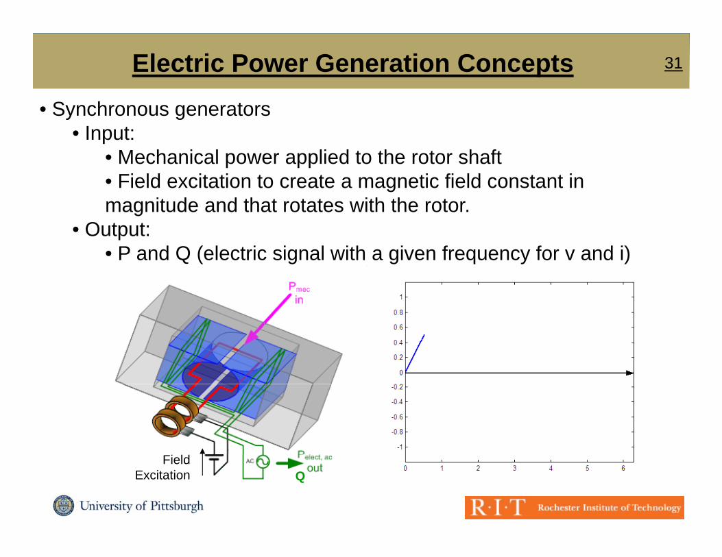
31Electric Power Generation ConceptsS h t• Synchronous generators
• Input: • Mechanical power applied to the rotor shaft
f• Field excitation to create a magnetic field constant in magnitude and that rotates with the rotor.
• Output:• P and Q (electric signal with a given frequency for v and i)
© A. Kwasinski, 2015
Field Excitation Q
32
Eff t f i fi ld it ti i h t
Electric Power Generation Concepts• Effect of varying field excitation in synchronous generators:
• When loaded there are two sources of excitation:• ac current in armature (stator)
f ( )• dc current in field winding (rotor)
• If the field current is enough to generate the necessary mmf, then no magnetizing current is necessary in the armature and the generator operates at unity power factor (Q = 0).• If the field current is not enough to generate the necessary mmf, then the armature needs to provide the additional mmf through a magnetizing current. Hence, it operates at an inductive power factor and it is said to be underexcited.p• If the field current is more than enough to generate the necessary mmf, then the armature needs to provide an opposing mmf through a magnetizing current of opposing phase. Hence, it
© A. Kwasinski, 2015
g g g pp g p ,operates at a capacitive power factor and it is said to be overexcited.
33
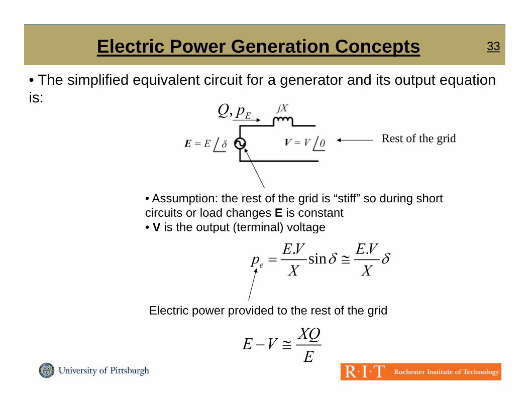
Th i lifi d i l t i it f t d it t t ti
Electric Power Generation Concepts• The simplified equivalent circuit for a generator and its output equation is:
, EQ p
Rest of the grid
• Assumption: the rest of the grid is “stiff” so during short circuits or load changes E is constant• V is the output (terminal) voltage
. .sineE V E VpX X
V is the output (terminal) voltage
Electric power provided to the rest of the grid
XQ
© A. Kwasinski, 2015
XQE VE

34
It b f d th t
Electric Power Generation Concepts• It can be found that
( ) synd tdt
• Generator’s angular frequency(rotor’s speed)
dt• Grid’s angular frequency
• Output frequency of a generator is proportional to its rotor angular velocity.• Ideally, the electrical power equals the mechanical input power. The generator’s frequency depends dynamically on δ which, in turn, depends on the electrical power (ideally it equals the input mechanical power). So by changing the mechanical power, we can p ) y g g pdynamically change the frequency.• Likewise, the reactive power controls the output voltage of the generator. When the reactive power increases the output voltage
© A. Kwasinski, 2015
g p p gdecreases.
35Voltage and frequency controlM t hi ti d d d ( l l ) i ti l f• Matching generation and demand (plus losses) is essential for power
grid stability. If generation is less than demand, frequency drops. If demand is less than generation, frequency increases.• Additionally, voltage needs to be controlled within a given range• To achieve these goals in an economically optimal way, power grids control system is structured in mainly 3-levels.
• Primary control: Local control using locally measured variables. Main goal: adjust electrical power output (i.e. adjust mechanical power input) to compensate for mismatches between generation and demand.• Secondary control: Local control using locally measured variables. Main goal: frequency (or voltage in some cases) regulation to a given g q y ( g ) g gnominal set point.• Tertiary control: Performed at a central location. Main goal: determine operation nominal set points in order for optimal operation.
© A. Kwasinski, 2015
p p p p• Primary control is often implemented through droop controllers.
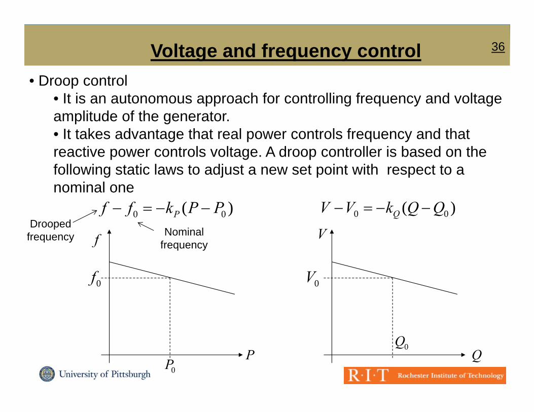
36Voltage and frequency controlD t l• Droop control
• It is an autonomous approach for controlling frequency and voltage amplitude of the generator.
f• It takes advantage that real power controls frequency and that reactive power controls voltage. A droop controller is based on the following static laws to adjust a new set point with respect to a nominal one
0 0( )Pf f k P P 0 0( )QV V k Q Q
VNominalDrooped
0f
f
0V
VNominal frequency
frequency
0f 0
© A. Kwasinski, 2015
P0P
Q0Q

37Voltage and frequency controlD t l• Droop control
•Then a simple (e.g. PI) controller can be implemented. It considers a reference voltage and a reference frequency:
f ff f•If the output voltage is different, the field excitation is changed (and, thus, changes Q and then V).
•If the frequency is different, the prime mover torque is changed (and thus, changes P and then f).
0 0( )Pf f k P P 0 0( )QV V k Q Q
f V
0f
f
0V
© A. Kwasinski, 2015
P0P
Q0Q
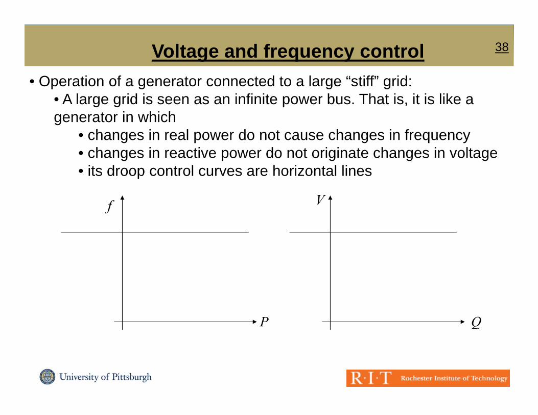
38Voltage and frequency controlO ti f t t d t l “ tiff” id• Operation of a generator connected to a large “stiff” grid:
• A large grid is seen as an infinite power bus. That is, it is like a generator in which
f• changes in real power do not cause changes in frequency• changes in reactive power do not originate changes in voltage• its droop control curves are horizontal lines
f V
P Q
© A. Kwasinski, 2015

39Voltage and frequency control• Real grids are not ideally “stiff” so frequency can changeReal grids are not ideally stiff so frequency can change.• In large grids with many generators with a high inertia and normal load changes frequency changes relatively slowly. However, frequency changes faster than changes in generators rotational speed (because ofchanges faster than changes in generators rotational speed (because of the relatively high inertia). So,
• when the load changes, the grid frequency changes toogrid frequency changes, too.
• when the frequency changes,the primary droop controlleradjusts the generator outputadjusts the generator outputto match generation anddemand based on the newffrequency.
• If there is a sufficiently large mismatch between generation and d d th t t b t d ith d t ll
© A. Kwasinski, 2015
demand that cannot be compensated with a droop controller, stability can be lost and the system may collapse.
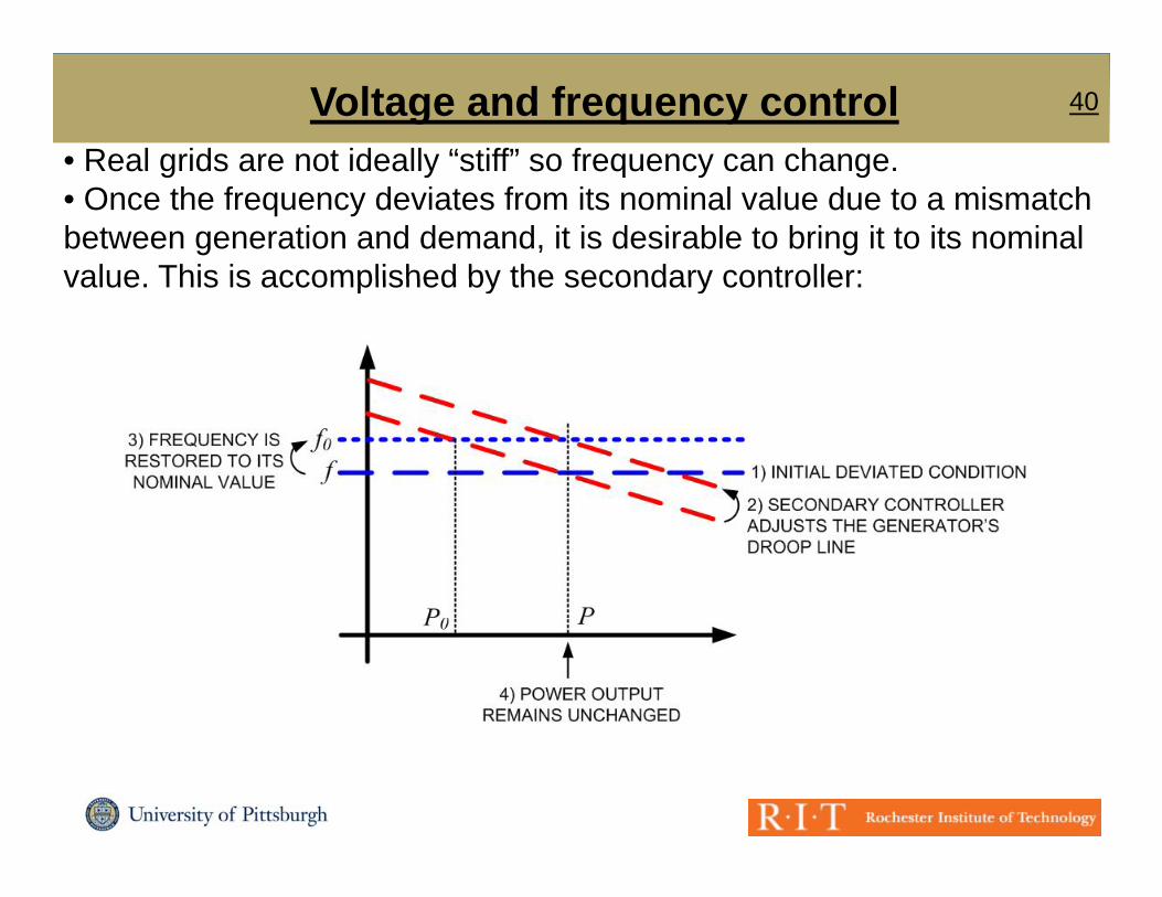
40Voltage and frequency control• Real grids are not ideally “stiff” so frequency can changeReal grids are not ideally stiff so frequency can change.• Once the frequency deviates from its nominal value due to a mismatch between generation and demand, it is desirable to bring it to its nominal value This is accomplished by the secondary controller:value. This is accomplished by the secondary controller:
© A. Kwasinski, 2015
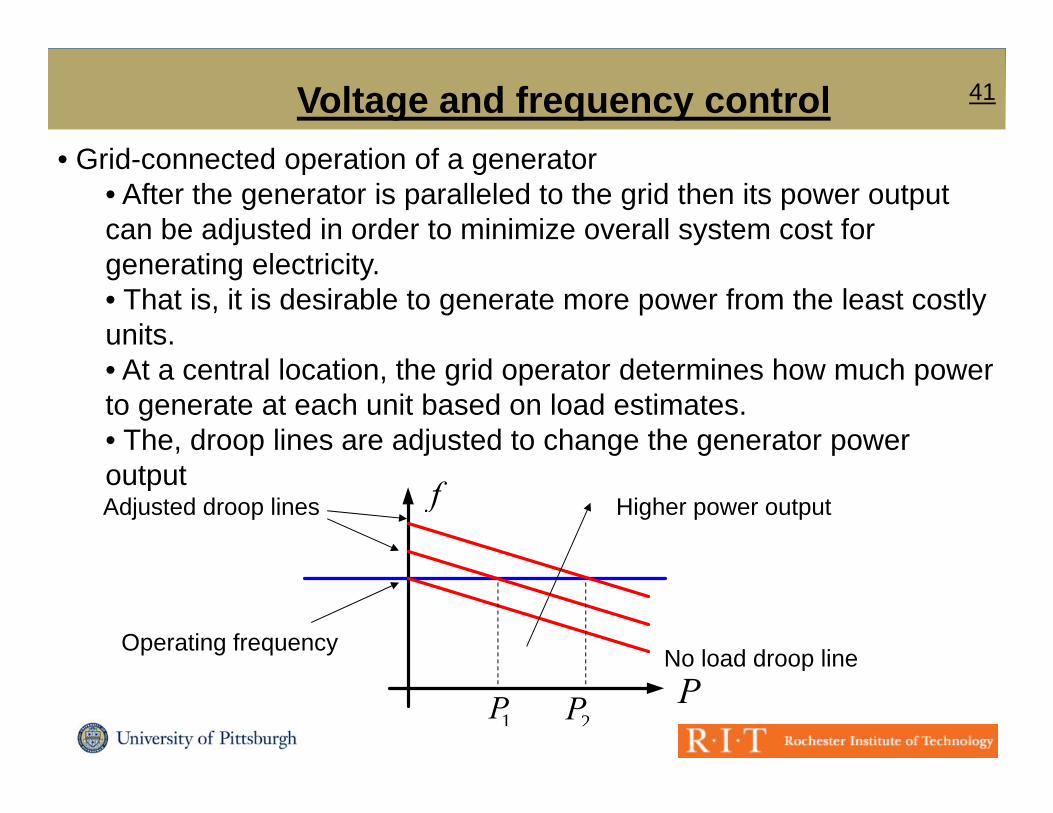
41Voltage and frequency controlG id t d ti f t• Grid-connected operation of a generator
• After the generator is paralleled to the grid then its power output can be adjusted in order to minimize overall system cost for generating electricity. • That is, it is desirable to generate more power from the least costly units.• At a central location, the grid operator determines how much power to generate at each unit based on load estimates. • The, droop lines are adjusted to change the generator power output fAdjusted droop lines Higher power output
Operating frequencyNo load droop line
© A. Kwasinski, 20152P1P P
No load droop line
42Additional commentsI ti l id l hi i ti h l t• In conventional ac grids, large machine inertia helps to maintain stability.
Si f d t b l t d t i l• Since frequency needs to be regulated at a precise value, imbalances between electric and mechanical power may make the frequency to change. In order to avoid this issue, mechanical power applied to the generator rotor must follow load changes.
• The same approach described with real power output can be used to adjust reactive power based on voltage regulation.
• Droop control is an effective decentralized controller.
• Optimal operation set points need to be transmitted from the t l ti t t th t
© A. Kwasinski, 2015
central operations center to the generators.
43Additional comments• Operation and monitoring of electric power grids is usually• Operation and monitoring of electric power grids is usually
performed with a SCADA (supervisory control and data acquisition) system. At a basic level a SCADA system includes:• Remote terminals• Central processing unit• Central processing unit• Data acquisition (sensing) units• TelemetryTelemetry• Human interfaces (usually computers).
• SCADA systems require communication links but, usually, these are dedicated links separate from the public communication networks used by people for their every day
© A. Kwasinski, 2015
communication networks used by people for their every day lives.

44Additional comments• Operating a power grids involves dealing with a broad time• Operating a power grids involves dealing with a broad time
scale range:
© A. Kwasinski, 2015
Source: NERC