Embed Size (px)
DESCRIPTION
ABOUT CVT
Citation preview

Thesis
Efficiency optimization of thepush-belt CVT by variator slip
control
B. Bonsen

A catalogue record is available from the Library Eindhoven University of Technology.
ISBN-10: 90-386-3048-4 ISBN-13: 978-90-386-3048-9
This thesis was prepared using the LATEX documentation system
Cover design by B. Bonsen Printed by Universiteitsdrukkerij, Technische Universiteit Eindhoven Copyright © 2006 by B. Bonsen All rights reserved. No parts of this publication may be reproduced or utilized in any form or by any means, electronic or mechanical, including photocopying, recording or by any information storage and retrieval system, without written permission of the copyright holder.

Efficiency optimization of the push-belt CVT by variator slip control
PROEFSCHRIFT
ter verkrijging van de graad van doctor aan de Technische Universiteit Eindhoven, op gezag van de Rector Magnificus, prof.dr.ir. C.J. van Duijn, voor een
commissie aangewezen door het College voorPromoties in het openbaar te verdedigen
op woensdag 13 december 2006 om 14.00 uur
door
Bram Bonsen
geboren te Amersfoort

Dit proefschrift is goedgekeurd door de promotor:
prof.dr.ir. M. Steinbuch
Copromotor:dr. P.A. Veenhuizen

Preface
This thesis is part of the result of a project jointly executed by three PhD students. In the followingtext the project and the project context will be briefly introduced, as well as the overall goals of theproject and the strategy to attain these goals.
The projectThe project is started in cooperation with three parties: the Technische Universiteit Eindhoven
(TU/e), Van Doorne’s Transmissie (VDT) and the University of Twente (UT). Each of these partiesundertakes a part of the project. The project is organized within the BTS (Bedrijfs TechnologischeSamenwerking) framework. In this framework companies and universities work together on projectsthat can stimulate economic development in the future.The project is divided into three sub-projects. Each sub-project focusses on one research topic andis carried out by one of the participants:
1. develop a model that describes the micro-slip behavior in a variator and translate this intoa dynamic measurement method. The aim of this topic is to improve the efficiency anddurability of the variator (TU/e),
2. develop new materials that combine high breaking strength with good fatigue resistance andare ground breaking for both properties (VDT),
3. develop a failure mode model and a wear prediction model for a boundary lubrication contact(UT).
The work in this thesis is part of the first topic, the micro-slip research performed by the TU/e. Thisresearch, performed in cooperation with VDT, focusses on the control and actuation of the variator.In this thesis only this part of the project will be discussed.
GoalsMost developments in the field of Continuously Variable Transmissions can be divided into five
areas of attention:
1. efficiency,
2. durability,
3. maximum torque,
4. costs and
5. driveability.
i
In this project the main focus is on efficiency, durability and maximum torque.The overall aim of the first research topic is to improve the efficiency and operability of the pushbelttype CVT. To achieve this, three subtargets can be formulated:
• Investigate methods to detect slip in a pushbelt type variator.
• Develop a control method to control slip in a pushbelt type variator.
• Investigate alternative actuation methods that will reduce the losses associated with the ac-tuation system in a CVT and increase the controllability of the variator.
This thesis addresses modeling and measurements characterizing slip in a pushbelt type variator,methods to detect slip in a pushbelt type variator as well as a control method to control slip in avariator. This thesis does not describe the Electro-Mechanical Pulley Actuation CVT (EMPAct CVT)[43] [86], which was also developed within the scope of this project.
ii

Contents
1 Introduction 11.1 CVT Drivelines . . . . . . . . . . . . . . . . . . . . . . . . . . . . . . . . . . . . . 2
1.1.1 CVT components . . . . . . . . . . . . . . . . . . . . . . . . . . . . . . . . 21.1.2 Belt types . . . . . . . . . . . . . . . . . . . . . . . . . . . . . . . . . . . . 41.1.3 Transmission load . . . . . . . . . . . . . . . . . . . . . . . . . . . . . . . 6
1.2 Driveline efficiency . . . . . . . . . . . . . . . . . . . . . . . . . . . . . . . . . . . 71.2.1 Driveability versus fuel economy . . . . . . . . . . . . . . . . . . . . . . . . 8
1.3 CVT efficiency . . . . . . . . . . . . . . . . . . . . . . . . . . . . . . . . . . . . . 81.3.1 Mechanical system efficiency . . . . . . . . . . . . . . . . . . . . . . . . . 91.3.2 Actuation system . . . . . . . . . . . . . . . . . . . . . . . . . . . . . . . . 9
1.4 Improvement strategy . . . . . . . . . . . . . . . . . . . . . . . . . . . . . . . . . 111.4.1 Alternative actuation system . . . . . . . . . . . . . . . . . . . . . . . . . . 111.4.2 Clamping force reduction . . . . . . . . . . . . . . . . . . . . . . . . . . . 121.4.3 Improvement potential . . . . . . . . . . . . . . . . . . . . . . . . . . . . . 12
1.5 Contribution of this thesis . . . . . . . . . . . . . . . . . . . . . . . . . . . . . . . 121.6 Outline of this thesis . . . . . . . . . . . . . . . . . . . . . . . . . . . . . . . . . . 13
2 Variator Modeling 152.1 Introduction . . . . . . . . . . . . . . . . . . . . . . . . . . . . . . . . . . . . . . . 16
2.1.1 Variator geometry . . . . . . . . . . . . . . . . . . . . . . . . . . . . . . . 172.1.2 Models . . . . . . . . . . . . . . . . . . . . . . . . . . . . . . . . . . . . . 19
2.2 Stationary Variator Modeling . . . . . . . . . . . . . . . . . . . . . . . . . . . . . . 222.2.1 Continuous belt model . . . . . . . . . . . . . . . . . . . . . . . . . . . . . 222.2.2 Pushbelt model . . . . . . . . . . . . . . . . . . . . . . . . . . . . . . . . . 332.2.3 Forces in the pushbelt . . . . . . . . . . . . . . . . . . . . . . . . . . . . . 342.2.4 Conclusion stationary model . . . . . . . . . . . . . . . . . . . . . . . . . . 40
2.3 Variator Transient Model . . . . . . . . . . . . . . . . . . . . . . . . . . . . . . . . 412.3.1 Creep-mode shifting . . . . . . . . . . . . . . . . . . . . . . . . . . . . . . 412.3.2 Slip-mode shifting . . . . . . . . . . . . . . . . . . . . . . . . . . . . . . . 412.3.3 Models . . . . . . . . . . . . . . . . . . . . . . . . . . . . . . . . . . . . . 422.3.4 Measurements . . . . . . . . . . . . . . . . . . . . . . . . . . . . . . . . . 432.3.5 Comparison . . . . . . . . . . . . . . . . . . . . . . . . . . . . . . . . . . 47
3 Slip in the variator 493.1 Slip and Traction . . . . . . . . . . . . . . . . . . . . . . . . . . . . . . . . . . . . 49
3.1.1 Traction curve . . . . . . . . . . . . . . . . . . . . . . . . . . . . . . . . . 503.1.2 Play in the belt . . . . . . . . . . . . . . . . . . . . . . . . . . . . . . . . . 513.1.3 Results . . . . . . . . . . . . . . . . . . . . . . . . . . . . . . . . . . . . . 54
3.2 Dynamic Variator Slip Model . . . . . . . . . . . . . . . . . . . . . . . . . . . . . . 553.3 Ratio and Slip Estimation . . . . . . . . . . . . . . . . . . . . . . . . . . . . . . . 58
3.3.1 Estimation vs Measurement . . . . . . . . . . . . . . . . . . . . . . . . . . 583.3.2 Position measurement . . . . . . . . . . . . . . . . . . . . . . . . . . . . . 59
iii

3.3.3 Input/Output torque . . . . . . . . . . . . . . . . . . . . . . . . . . . . . . 593.3.4 Beltspeed . . . . . . . . . . . . . . . . . . . . . . . . . . . . . . . . . . . . 613.3.5 Modulation methods . . . . . . . . . . . . . . . . . . . . . . . . . . . . . . 623.3.6 Results . . . . . . . . . . . . . . . . . . . . . . . . . . . . . . . . . . . . . 66
4 Variator system losses 694.1 Losses . . . . . . . . . . . . . . . . . . . . . . . . . . . . . . . . . . . . . . . . . 69
4.1.1 Efficiency of the variator . . . . . . . . . . . . . . . . . . . . . . . . . . . . 704.1.2 Losses in the hydraulic actuation system . . . . . . . . . . . . . . . . . . . 704.1.3 Losses in the variator . . . . . . . . . . . . . . . . . . . . . . . . . . . . . 70
4.2 Measurements . . . . . . . . . . . . . . . . . . . . . . . . . . . . . . . . . . . . . 714.3 Torque loss . . . . . . . . . . . . . . . . . . . . . . . . . . . . . . . . . . . . . . . 714.4 Results . . . . . . . . . . . . . . . . . . . . . . . . . . . . . . . . . . . . . . . . . 744.5 Efficiency improvement potential . . . . . . . . . . . . . . . . . . . . . . . . . . . 744.6 Conclusions variator efficiency . . . . . . . . . . . . . . . . . . . . . . . . . . . . 76
5 CVT Control 795.1 Control problem . . . . . . . . . . . . . . . . . . . . . . . . . . . . . . . . . . . . 805.2 Classic Clamping-force Control . . . . . . . . . . . . . . . . . . . . . . . . . . . . 805.3 Ratio control . . . . . . . . . . . . . . . . . . . . . . . . . . . . . . . . . . . . . . 825.4 Slip Control . . . . . . . . . . . . . . . . . . . . . . . . . . . . . . . . . . . . . . . 825.5 Simulation . . . . . . . . . . . . . . . . . . . . . . . . . . . . . . . . . . . . . . . 865.6 Conclusions and recommendations variator control . . . . . . . . . . . . . . . . . 88
6 First generation slip controlled variator 916.1 Experimental setup . . . . . . . . . . . . . . . . . . . . . . . . . . . . . . . . . . 916.2 Control implementation . . . . . . . . . . . . . . . . . . . . . . . . . . . . . . . . 93
6.2.1 Introduction . . . . . . . . . . . . . . . . . . . . . . . . . . . . . . . . . . . 936.2.2 System identification . . . . . . . . . . . . . . . . . . . . . . . . . . . . . . 936.2.3 Controller tuning . . . . . . . . . . . . . . . . . . . . . . . . . . . . . . . . 94
6.3 Experimental results . . . . . . . . . . . . . . . . . . . . . . . . . . . . . . . . . . 956.4 Conclusions and recommendations first implementation . . . . . . . . . . . . . . . 96
7 Gain scheduled PI control of slip in a CVT 997.1 Transmission testrig . . . . . . . . . . . . . . . . . . . . . . . . . . . . . . . . . . 997.2 Control implementation . . . . . . . . . . . . . . . . . . . . . . . . . . . . . . . . 100
7.2.1 Slip model . . . . . . . . . . . . . . . . . . . . . . . . . . . . . . . . . . . 1007.3 Experimental results . . . . . . . . . . . . . . . . . . . . . . . . . . . . . . . . . . 1077.4 Conclusions and recommendations gain scheduled PI control . . . . . . . . . . . . 109
8 Implementation of slip control in a production vehicle 1118.1 Nissan Primera . . . . . . . . . . . . . . . . . . . . . . . . . . . . . . . . . . . . . 111
8.1.1 Engine . . . . . . . . . . . . . . . . . . . . . . . . . . . . . . . . . . . . . 1118.1.2 Transmission control . . . . . . . . . . . . . . . . . . . . . . . . . . . . . . 1128.1.3 Clamping force control . . . . . . . . . . . . . . . . . . . . . . . . . . . . . 1128.1.4 Variator Properties . . . . . . . . . . . . . . . . . . . . . . . . . . . . . . . 113
8.2 Variator Robustness . . . . . . . . . . . . . . . . . . . . . . . . . . . . . . . . . . 1138.3 Comfort . . . . . . . . . . . . . . . . . . . . . . . . . . . . . . . . . . . . . . . . . 1168.4 Conclusions and recommendations Nissan Primera tests . . . . . . . . . . . . . . 117
9 Conclusions and Recommendations 1199.1 Conclusions . . . . . . . . . . . . . . . . . . . . . . . . . . . . . . . . . . . . . . 1199.2 Recommendations . . . . . . . . . . . . . . . . . . . . . . . . . . . . . . . . . . . 121
iv

A Slip control using Linearizing and decoupling feedback 123A.1 Linearizing and decoupling feedback . . . . . . . . . . . . . . . . . . . . . . . . . 123
A.1.1 Linearizing feedback . . . . . . . . . . . . . . . . . . . . . . . . . . . . . . 123A.1.2 Decoupling feedback . . . . . . . . . . . . . . . . . . . . . . . . . . . . . . 124
A.2 Controller design . . . . . . . . . . . . . . . . . . . . . . . . . . . . . . . . . . . . 124A.3 Conclusions and recommendations linearizing and decoupling feedback . . . . . . 126
B Equations 127B.1 System matrices for the linearized model . . . . . . . . . . . . . . . . . . . . . . . 127B.2 Iterative calculation of the wrapped angle and running radii . . . . . . . . . . . . . 128B.3 Quadratic approximation of the wrapped angle and running radii . . . . . . . . . . . 129
C Robust PI Control 131
D Drive cycles 133D.1 NEDC . . . . . . . . . . . . . . . . . . . . . . . . . . . . . . . . . . . . . . . . . 133D.2 FTP75 . . . . . . . . . . . . . . . . . . . . . . . . . . . . . . . . . . . . . . . . . 135
E Ratio Setpoint Strategy 137E.1 Optimal Operation Line . . . . . . . . . . . . . . . . . . . . . . . . . . . . . . . . 138E.2 Drivability . . . . . . . . . . . . . . . . . . . . . . . . . . . . . . . . . . . . . . . . 138
E.2.1 Shiftspeed . . . . . . . . . . . . . . . . . . . . . . . . . . . . . . . . . . . 140
Bibliography 143
Nomenclature 151
Summary 157
Samenvatting 159
Curriculum Vitae 161
v

vi

Chapter 1
Introduction
The Continuously Variable Transmission (CVT) is increasingly used in automotive applications. It
has an advantage over conventional automatic transmissions, with respect to the large transmis-
sion ratio coverage and absence of comfort issues related to shifting events. This enables the
engine to operate at more economic operating points. For this reason, CVT equipped cars are
more economical than cars equipped with planetary gear automatic transmissions. Despite these
advantages, V-belt type CVT’s still have rather large potential in transmission efficiency, as can be
seen in Figure 1.1. Also torque capacity (currently at about 350 Nm) needs expansion.
Recent developments in the field of automatic transmissions include Automated Manual Trans-
missions (AMT), Dual Clutch Transmissions (DCT) and the Electronic CVT (eCVT) developed for
the Toyota hybrid cars. Although the AMT is very efficient with respect to transmission efficiency,
the AMT has a disadvantage with respect to CVTs with regard to driveability. Shifting in AMTs
causes a discontinuity in the driving torque. The DCT solves this problem by using an additional
clutch and driveshaft. This however, increases the cost of the system. The eCVT uses an electric
motor and a generator combined with a planetary gear to drive the wheels. This is an interesting
Figure 1.1: The efficiency of a reference CVT set against the efficiency of a manual transmission.
1
Chapter 1 Introduction
option, because there is an additional benefit of an electric power buffer. This greatly improves fuel
economy, but at the same time also greatly increases the cost of the system.
New systems with increasing numbers of gears of up to 8 gears in the latest automatic gearbox
decrease the advantage of the CVT with respect to the transmission ratio coverage and optimal
engine operation (i.e. fuel economy). However, the increasing number of gears present additional
costs and increased size of the transmissions. The pushbelt type CVT already has a large ratio
coverage and unlimited number of gears.
As stated before, the main disadvantages of current CVTs are transmission efficiency and torque
capacity. Therefore development of these systems is mainly focussed in these areas.
This thesis proposes to use control of slip in a pushbelt type Continuously Variable Transmission.
It will be shown that control of slip in such a CVT can be used to optimize the efficiency of a CVT.
Models will be given for the forces, shifting behavior, slip and efficiency of the variator. The variator
is the ratio changing device of the CVT. Several methods to estimate slip in a CVT will be discussed.
Furthermore, a controller will be proposed that can be used to control slip in a CVT. A functional
prototype has been produced and the results from tests with this prototype will also be discussed.
A general introduction on CVT drivetrains will be given in order to describe the main focus points of
this research.
1.1. CVT Drivelines
The CVT will be discussed in the form in which it is used the most: transversely mounted in a front
wheel driven car. The driveline contains an internal combustion engine, a transmission, and drive
shafts to the wheels. (Figure 1.2)
1.1.1. CVT components
The CVT consists of several components, i.e. an actuation system, a launching device, a drive-
neutral-reverse set, a variator and a final drive reduction. These parts are discussed briefly here.
Launching device
A CVT needs a separate device for launching. Often a torque converter (TC) is used for this
purpose. After vehicle launch, the TC can be locked by engaging the lock-up clutch. It then forms
a fixed connection between the engine and the rest of the transmission. These components and
their models are described in more detail in Serrarens [70], Lechner et al. [48] and B. Bertsche et
al. [6].
2

1.1 CVT Drivelines
IC EngineCVT
DNR
Torque converterVariator
Drive shaft
Wheel
Differential
Final drive reduction
Oil pump
Figure 1.2: Driveline Components
Drive-Neutral-Reverse set
To enable the driver to put the driveline in neutral or to select forward or reverse driving, the CVT
contains a Drive-Neutral-Reverse (DNR) set. The DNR consists of a planetary gear set and two
wet plate clutches. The clutches can either couple the planet carrier to the transmission housing
(Reverse) or the ring gear to the planet carrier (Drive). If none of the clutches is engaged, the
transmission is in neutral.
Variator
The variator consists of a segmented steel V-belt and two shafts with conical pulleys, that forms
the heart of the CVT. The belt is clamped between two pairs of conical sheaves. In the variator
the transmission ratio is determined by simultaneous adjustment of the running radii of the belt on
the pulleys. On each shaft, there is one fixed and one axially moveable sheave. Axial movement
of the moveable sheave adjusts the gap between the sheaves and thereby the belt running radius.
The input shaft of the variator is called the primary shaft, the output shaft is he secondary shaft. In
Figure 1.3 the working principle of the variator is illustrated. In this figure the shifting process from
the low ratio to overdrive ratio is shown. Here the front shaft is the input shaft.
Final drive reduction
The secondary shaft of the variator is connected to the differential gear via a number of gears.
The differential gear distributes the torque between the two drive shafts. Together, the gears on
the secondary variator shaft, the intermediate shaft and the differential gear form the Final Drive
Reduction, or FDR. The wheels rotate in the same direction as the engine when the DNR is in
Drive.
3

Chapter 1 Introduction
Low Medium Overdrive
Figure 1.3: The working principle of the V-belt type variator illustrated by the shifting process from
low ratio to overdrive ratio.
Actuation system
Early CVTs used a mechanical system to control clamping force and ratio [24]. The efficiency
and driveability however were very poor. To achieve better controllability, hydraulic systems were
developed. The advantages are a high power density and control of the speed ratio independent of
the shaft speeds.
In current CVT systems the clamping force is delivered by a hydraulic actuation system. Also
mechanical systems (torque cams) and electromechanical systems, for example the EMPAct CVT
[86], are possible.
For a hybrid vehicle application, a CVT with electro-hydraulic actuation was developed [33]. In
this setup, an electric motor drives the hydraulic system’s oil pump. This is necessary in hybrid
vehicles, since the IC engine is occasionally shut down and can not be used to continuously drive
the oil pump.
Recently attention has been given to electro-mechanical systems. Aichikikai developed such a
system for dry hybrid belts [83]. The EMPAct, developed at the TU Eindhoven, also is an electro-
mechanically actuated CVT for metal pushbelts.
1.1.2. Belt types
The belt appears in several forms. The most important belt types are:
• the dry belt,
• the chain and
• the pushbelt.
4

1.1 CVT Drivelines
Figure 1.4: Dry belt CVT as produced by Aichikikai
Dry Belt
The development of the V-belt type CVT began with rubber V-belts [24]. This type of CVT is
still being developed and used. However, rubber V-belt CVTs are not well suited for automotive
applications, because of their limited torque capacity. Nevertheless, there are some interesting
concepts on the market, for example the Bando Avance system [83]. Dry belts are of interest
because a much higher friction coefficient is established between belt and pulleys than in lubricated
variants. A dry belt CVT therefore needs less clamping force and can be much smaller and lighter.
This is interesting for low power applications, such as light motorcycles and small cars.
A problem that arises from the non-lubricated belt pulley contact is that there is no cooling of this
contact by lubrication oil. This greatly limits the torque capacity of this type of variator. A picture of
a dry V-belt CVT [83] is given in Figure 1.4.
Chain
CVT chains as developed by Luk [51] or GCI [91] consist of pins and segments. The pins are
typically crowned to enhance the chain-pulley contact. Most CVT chains only have rolling contacts
between the pins and have static contacts between the pins and the segments.
The chains have very little internal friction due to their internal rolling contacts (i.e. no sliding con-
tacts). The efficiency of the chains compared to pushbelts is therefore generally higher, especially
for low input torques.
Figure 1.5 gives a picture of the Luk CVT chain. This chain uses two pins per section. The pins
of the chain are grouped two by two. This enables the chain to transmit the tension force by rolling
and static contacts only, i.e. no sliding occurs in the chain. However, the pins need to rotate in order
to change the configuration of the chain. When compressed between the pulley sheaves, this will
cause a counteracting friction between the pulley and the pins. The GCI chain solves this problem
by shortening one pin slightly, eliminating this friction. A disadvantage is that the number of pins is
effectively halved, lowering the stiffness and the strength.
5

Chapter 1 Introduction
Figure 1.5: A Luk CVT chain
Typically chains produce more noise than pushbelts. This is caused by the relatively small number
of pins that continuously run into the pulley. Luk overcomes this problem by varying the length of
the segments. This causes the system to make noise in a wider frequency band, but with a lower
amplitude [38]. GCI claims that their chain causes less noise than the Luk chain, because of the
eliminated rotation under load.
Pushbelt
The Van Doorne’s Transmissie pushbelt consists of blocks and bands as shown in Figure 1.6. The
bands, normally 2 sets of between 9 and 12 bands each, fit tightly together, holding the blocks
together. The bending stiffness of the bands is very small and may be neglected, so that only a
tension force can be present in the bands. The blocks can transmit torque when they are under
compression, hence the name pushbelt. The compression force can never exceed the tension in
the bands, otherwise the contact between the pushbelt and the pulleys could be lost and buckling
could occur.
Apart from the losses in the bearings of the shafts and losses due to slip, there are friction losses in
the pushbelt. The bands and the blocks do not run at the same radius, causing a speed difference
between the blocks and the bands. This results in friction losses in the pushbelt, which lowers the
efficiency of the pushbelt.
Because of the continuous bending and stretching of the bands, fatigue issues are important.
Fatigue resistance specifications limit the torque capacity of the variator, because the maximum
clamping forces are limited.
There are much more blocks in a pushbelt than there are pins in a chain. This results in more quiet
operation and higher axial stiffness. Also better resistance to wear is achieved due to the lower
surface pressure between pushbelt and pulley.
1.1.3. Transmission load
At the input or engine side, the transmission is loaded with the engine torque. In a typical medium-
size car, the maximum engine torque can vary between different types, but is roughly somewhere in
6

1.2 Driveline efficiency
Figure 1.6: A metal pushing V-belt
the 150-350 Nm range. Engine torque changes can be highly dynamic, from no load to maximum
torque in half a crankshaft rotation. The engine torque is filtered by a torsion damper. The engine
torque can also be amplified by a torque converter.
At the output side, the transmission is loaded by the torque in the drive shafts. Apart from the reac-
tion torque of up to 2500 Nm that results from the engines driving torque, torque peaks can occur
resulting from hitting a curbstone, abruptly stopping of spinning wheels or other events occurring in
the road-wheel contact.
1.2. Driveline efficiency
Figure 1.7(a) shows the energy flow in a CVT driveline. The output in the CVT driveline is about
the same as the output of a manual transmission driveline [62]. For this driveline the energy flow is
shown in Figure 1.7(b). The CVT losses are higher, but the engine losses are less than the losses
with a manual gearbox. The transmission is assumed to have an average efficiency of around 80%
in the CVT driveline. CVT main loss components are the variator loss and the hydraulic loss [35].
The main reason for the low efficiency of modern production CVTs is the high clamping force
necessary to transfer the engine torque. To prevent belt slip at all times, the clamping forces in
modern production CVTs are usually much higher (at least 30% or more) than needed for normal
operation, i.e. without disturbances. Higher clamping forces result in higher losses in both the
hydraulic and the mechanical system, i.e. increased pump losses and increased friction losses
because of the extra mechanical load that is applied on all variator parts.
Excess clamping forces also reduce the endurance of the belt, since the net pulling force in this
element is larger than strictly needed for the transfer of the engine power. Also the contact pressure
between V-belt and sheaves is higher than strictly needed, leading to increased wear. This excess
loading leads to heavier components, thereby compromising power density.
7

Chapter 1 Introduction
0 0.5 1 1.5 2 2.5 3 3.5 4−1
−0.5
0
0.5
1
1.5
2
Engine losses (60%)
Transmission losses (8%)
Wheels (32%)
(a) Energy flow in a CVT Driveline
0 0.5 1 1.5 2 2.5 3 3.5 4−1
−0.5
0
0.5
1
1.5
2
Engine losses (65%)
Transmission losses (1.75%)
Wheels (33.25%)
(b) Energy flow in a manual transmission Driveline
Figure 1.7: Energy flows in different drivelines
1.2.1. Driveability versus fuel economy
For every power level in an internal combustion engine, there is one speed-torque combination
which achieves optimal fuel efficiency. If for all the engines power levels these points of optimal
efficiency are connected, a line appears that is called the optimal operation line, or OOL. With a
CVT, using its continuously variable range of transmission ratios, the OOL can be followed for high
driveline efficiency. If the driveline is operating in a low power situation and the driver demands
more power by pressing the accelerator pedal, the engine can be in a higher torque level within
half a crankshaft rotation. However, the torque reserve on the OOL is low, and much higher power
levels cannot be reached without increasing engine speed. This takes far more time than the
earlier mentioned increase in engine torque, because the CVT has to be shifted and the engines
inertia has to be accelerated. This time lag compromises the cars sporty feel and is regarded as a
driveability disadvantage. To counteract this, the CVT is usually operated in a lower transmission
ratio, letting the engine run below the OOL in a region with higher engine speed, larger torque
reserve and lower engine efficiency.
1.3. CVT efficiency
Improving CVT efficiency is a key factor in improving the fuel efficiency of CVT equipped vehicles.
Factors that influence the efficiency of the CVT are:
• Mechanical system efficiency,
• Actuation system losses,
• Control strategy.
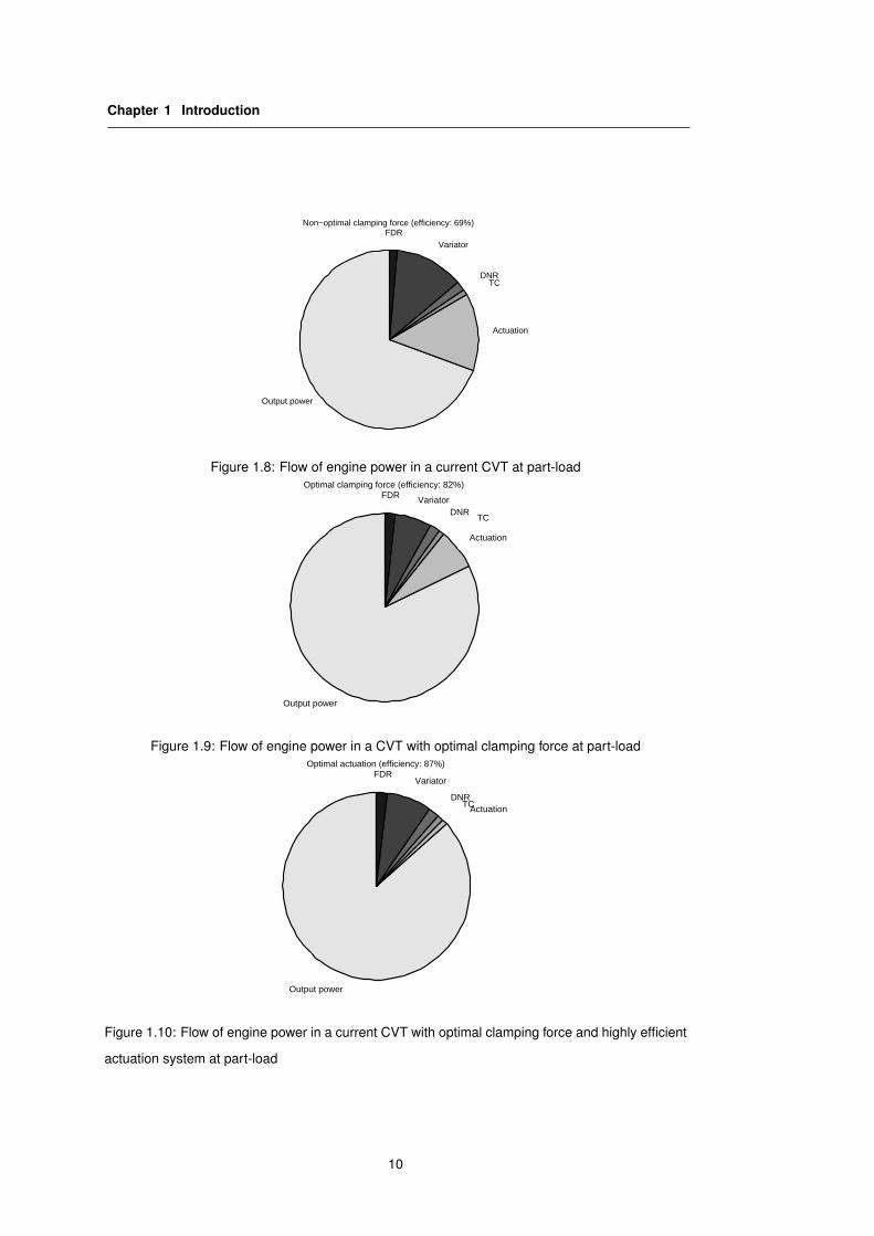
In Figure 1.8 the use of engine power in a typical CVT is shown when driving at constant moderate
speed. It can be seen that the actuation system takes a large part of the power and also that the
8

1.3 CVT efficiency
variator is not very efficient. If the clamping forces are lowered to the lowest possible value, the
efficiency of the CVT improves [10] [59]. This is shown in Figure 1.9. Not only the efficiency of the
variator improves, but also the power needed for the actuation system is decreased. However, the
actuation system still requires a significant amount of power. If the actuation system is made more
efficient this power can be reduced. The resulting power chart is shown in Figure 1.10. In total the
efficiency in the chosen operating point can be increased from circa 69% to circa 87%.
1.3.1. Mechanical system efficiency
The mechanical system of a CVT consists of shafts with bearings, gears, a variator and a launching
device, mostly a torque converter. The mechanical efficiency depends on the design and construc-
tion of these components, the clamping forces and the transferred torque.
Unlocked torque converters have a very limited power transmission efficiency. To overcome this
problem mostly a lock-up clutch is added. When this clutch is closed, the efficiency is equal to the
efficiency of the lock-up clutch. The Driveline Management System (DMS) therefore has to engage
the lock-up clutch as soon as possible after vehicle launch.
The lock-up clutch as well as the clutches in the DNR set are commonly of the wet-plate type. This
type usually has some slip when torque is transmitted. Although this slip is very small, it causes
the clutches to have a smaller than 100% efficiency.
The bearings on the primary and secondary shafts are heavily loaded in radial direction. This load
is caused by the tension in the belt, which in turn depends on the clamping forces. This load results
in friction losses in these bearings.
The torque transmission in the variator is based on friction and, similar to the clutches, this results
in some slip. The total amount of this speed-loss is the result of slip between the blocks and the
pulleys and between the blocks and the bands in the pushbelt. The power losses in the variator
depend linearly on the clamping forces.
The gears between the secondary shaft with the differential gearbox and the differential gears itself
cause some power losses in the transmission. All transmissions contain a differential gearbox, so
these losses are no issue if the performance of CVTs is compared to other types of transmissions.
1.3.2. Actuation system
The power to operate the actuation system of the CVT is taken from the drivetrain, so the power
requirement of this system decreases the efficiency of the CVT. Several actuation principles exist:
• Hydraulic actuation,
• Electro-hydraulic actuation,
• Electro-mechanical actuation.
9
Chapter 1 Introduction
Output power
Actuation
TC DNR
VariatorFDR
Non−optimal clamping force (efficiency: 69%)
Figure 1.8: Flow of engine power in a current CVT at part-load
Output power
Actuation
TC DNR
VariatorFDROptimal clamping force (efficiency: 82%)
Figure 1.9: Flow of engine power in a CVT with optimal clamping force at part-load
Output power
Actuation TC DNR
VariatorFDR
Optimal actuation (efficiency: 87%)
Figure 1.10: Flow of engine power in a current CVT with optimal clamping force and highly efficient
actuation system at part-load
10

1.4 Improvement strategy
Most present day production CVTs operate on hydraulic power, generated by an oil pump con-
nected directly to the input shaft. Normally this will be a pump with a constant flow per revolution.
The flow has to meet certain specifications in all driving situations and especially should be large
enough to operate the CVT at idle engine speed. Higher engine speeds cause the pump to gener-
ate too much flow for the CVT, increasing the actuation losses of the CVT. A better solution is found
in dual flow pumps, which can switch between a high- and a low-flow mode.
Another possibility is using an electro-hydraulic actuation system [72]. An electro-hydraulic actua-
tion system generates just enough flow to operate the CVT, but it needs an extra elektromotor.
Eliminating the hydraulic system altogether is possible using an electro-mechanical actuation sys-
tem [86]. This solution not only eliminates the excess oil-flow, but also eliminates the leakage in the
hydraulic cylinders.
1.4. Improvement strategy
To increase the efficiency of the CVT the most prominent power losses will be addressed in this
project. These are:
• Actuation system losses,
• Mechanical system losses.
As mentioned before, the actuation system losses can be lowered by lowering the clamping forces
and/or changing the design of the actuation system. Whereas the mechanical system losses can
be lowered by lowering the clamping forces and/or changing the design of the variator.
The design of the belt and the variator lies not within the scope of this project and therefore the
design of the actuation system and the level of the clamping forces are the issues to be investigated
in this project.
1.4.1. Alternative actuation system
To eliminate the excess flow from the hydraulic unit and to eliminate oil leakage from the hydraulic
cylinder in the variator, the approach is taken to use electro-mechanical instead of hydraulic ac-
tuation. The fuel saving potential of this approach is greater than that of electro-hydraulic and
alternative hydraulic actuation systems [45] [46].
An electro-mechanical actuation system can be designed to hold a prescribed ratio without power
consumption, using a self-braking (worm-wheel) transmission or to hold the ratio with a certain
motor torque. This last method has less friction and a faster response, but uses some power even
when not shifting.
Electro-mechanical systems can be much stiffer than low-pressure hydraulic systems. This is a
benefit for ratio and clamping force control. The electro-mechanical CVT developed by van de
Meerakker et al. [86], the EMPAct CVT, is an example of such a CVT.
11

Chapter 1 Introduction
1.4.2. Clamping force reduction
Current CVTs use over-clamping to avoid slip. Over-clamping means that more clamping force is
used than is necessary to transfer the input torque to the output shaft without excessive slip. This
over-clamping gives a margin of safety to overcome a priori unknown disturbances. Using more
clamping force than necessary also means more friction than necessary due to the higher forces.
Furthermore, the actuation system has to provide a higher force. In the case of hydraulic actuation
system this means flow at a higher pressure and thus higher losses.
To avoid over-clamping, an alternative method must be used to deal with the disturbances. If no
over-clamping is used, then every disturbance will cause severe slip events which could potentially
damage the variator [89]. Alternatively, measurements of the actual torque or of the slip in the
variator can be used to control the clamping force with lower or no over-clamping while reducing
the risk of excessive slip.
Lowering the safety margin and using feedback control will demand higher bandwidth for the clamp-
ing force actuation system.
1.4.3. Improvement potential
The potential improvement in terms of fuel economy depends on the driving conditions. In this
project the NEDC cycle (see also Appendix D) is used as a benchmark. The transmission efficiency,
however, is optimized over the whole working range of the CVT.
The improvement goals are:
• 10% overall improvement on the NEDC cycle,
• 25% less mechanical losses by clamping force reduction,
• 75% less actuation power needed by combining lower clamping forces with a highly efficient
actuation system.
The reference transmission used for the improvement comparison is the CK2 transmission from
Jatco [40]. This transmission is sold in high volumes throughout the world.
1.5. Contribution of this thesis
In this thesis the use of slip as the major control variable in a pushbelt type variator will be proposed
as a method to reduce the required clamping forces. If slip control is to be used, then a number
of questions need to be answered: what happens when a variator starts slipping, how can slip in
a CVT be measured or detected, how does slip influence the efficiency of the variator and can slip
in a variator be controlled in currently available automotive CVTs? These are questions that are
addressed in this thesis.
12

1.6 Outline of this thesis
Modeling and simulation combined with experimental data will be used to gain insight in the work-
ing principles of the variator, especially with respect to slip in this variator. Methods for estimating
the slip in a pushbelt type variator will be evaluated and a control law will be designed using these
models and the measurement data.
Models are shown for the torque transmission, for the variator transient behavior and the for slip.
Experimental data is obtained by numerous experiments on transmission testrigs and in test vehi-
cles. These tests give insight into the working principles of the V-belt type variator, provide input
data for the models and make it possible to evaluate these models.
The measurement data is used to determine the optimal operating point of a pushbelt type variator.
Measurements of the traction curve, i.e. plots of the transmitted torque versus slip, are combined
with measurements of the variator efficiency. Control of slip in a variator is enabled by accurate
estimation of slip and accurate models of the variator. Using the models, a method is developed to
accurately control the slip.
Simulations are used to evaluate the control method. These simulations give insight into the possi-
bilities of slip control without the limitation of one particular implementation. Apart from the simula-
tions, the proposed control method is implemented and tested in laboratory conditions and in two
test vehicles. Some results from these implementations will also be shown.
1.6. Outline of this thesis
The flowchart of the development process of the slip controlled CVT is graphically shown in Fig-
ure 1.11. First, fairly realistic, complex models are derived and evaluated, using data from exper-
iments on the reference transmission. Next, simplified models are used to design a controller for
slip in a variator. The designed controller is tested in simulations with the models and implemented
first on a beltbox testrig, then in a prototype transmission, and finally in a test vehicle, which are all
tested in the laboratory.
In Chapter 2 models for several aspects of the V-belt type variator will be discussed. Stationary
models for the forces in the belt and on the pulleys in stationary conditions (no shifting) and tran-
sient models describing the ratio changing behavior are presented.
In Chapter 3 a model for the slipping behavior of the variator will be discussed and several possible
methods are described to estimate the slip. These methods include pulley position measurement,
measurement of the running radius of the belt on the pulleys, torque measurement, belt speed
measurement and speed modulation methods.
In Chapter 4 an efficiency model describing the efficiency of the variator in all operating points will
be shown. The parameters for this model are derived from experimental data. From this data and
the model the optimal value for the slip in the variator can be obtained.
Chapter 5 describes the variator control problem. The classic clamping force control system is
reviewed. Simulations are shown illustrating the problems associated with clamping force control.
13

Chapter 1 Introduction
Reference
CVT Physical modelModeling forControl
SimulationControl systemdesignPrototype
reality virtual
Sec 2.1 Ch. 3, 4
Measurementsetup Estimation
Sec 5.5Ch. 8 Ch. 5, 6, 7, 9
Sec 3.3Chapter 6,7
Chapter 7
Figure 1.11: Information use in the design process
In Chapter 6 the first proposed slip control algorithm is evaluated. The test setup is discussed and
the design and implementation are explained. Some results are shown from the measurements.
In Chapter 7 the implementation on the transmission testrig in a production CVT is explained. The
design and implementation in this transmission is explained and the results are discussed.
Chapter 8 gives the experimental results of the implementation of slip control in the test vehicle, the
Nissan Primera, and gives an evaluation of the results.
Finally, some conclusions and recommendations are given in Chapter 9.
14
Chapter 2
Variator Modeling
Understanding of the basic mechanical properties of the V-belt variator is essential to improve its
performance. Modeling the variator can give this insight and the resulting models can be used to
study the influences of the design parameters of the variator. For controller design and verification,
especially for the control of the transmission ratio and for variator simulation, models of the station-
ary and transient behavior of the variator are needed. The clamping forces and especially the ratio
of clamping forces are of interest here, therefore the forces in the variator will be studied in this
chapter.
In Section 2.1 a general introduction is given to the principles of the V-belt type variator. An overview
of the literature on this topic is given. Next, the geometry of the variator is discussed. Because of
the importance of friction in variators, a few friction models are discussed. These friction models
will be compared in the belt model in Section 2.2.
In Section 2.2 the clamping force ratio for stationary conditions, i.e. when the variator is not shift-
ing, is studied. Two models will be presented, a continuous belt model and a pushbelt model. A
parameter sensitivity analysis and an experimental model verification will be given for both models.
In Section 2.3 the shifting behavior of the variator is discussed. Several models from literature will
be described. A qualitative comparison of these models will be given and experimental data will be
shown.
Models for other drivetrain components found in common CVT drivetrains are described for exam-
ple by Lechner and Naunheimer [6] and by Serrarens [70].
Although models that describe continuous belts and chains will be discussed, all measurements
have been performed on the metal pushing V-belt of Van Doorne’s Transmissie. Although focus
of this research is on this type of belt, the continuous belt model that will be described, is also
applicable to other types of belts or chains.
15

Chapter 2 Variator Modeling
2.1. Introduction
The variator of a CVT is a device that uses friction to transmit power from a driving pulley set to
a belt and then from the belt to the driven pulley set. The interaction between pulleys and belt
determines the forces acting on the pulleys and the belt. These forces cause bending of the pulleys
and shafts and elongation of the belt.
This deformation of pulleys and belt influence the efficiency and power transmission of the varia-
tor. For controller design and verification the clamping forces needed for torque transfer and ratio
changing and the relation between clamping force and efficiency are important.
Because of the friction and of the various finite stiffnesses involved, the power transmitting mech-
anism of a variator poses a mathematically complex modeling problem. Most models take only
a part of the mechanism into account. For example Gerbert [31] and Van Rooij [92] assume the
pulleys and belts to be rigid. Also they assume the friction force to behave like Coulomb friction.
Kobayashi [47] and Asayama [5] have proposed models for pushbelt type variators. In their models
they assume rigid pulley sheaves and rigid blocks and bands in the pushbelt. The main difference
with the continuous belt models is the compression force that is present between the blocks of the
pushbelt.
Others include a model for the flexibility of the pulleys like Srnik and Pfeiffer [79], Tenberge [84] and
Sattler [67]. Including the flexibility of the pulley increases the complexity of the model, but also
increases the accuracy of the results compared to measured data [84]. Modeling pulleys with finite
stiffness can be very complex and thus cause time consuming calculations. Tenberge [84] uses fi-
nite element analysis for calculating the bending of the pulley. Doing the finite element calculations
during the iterative calculation process would make this calculation very slow. To overcome this
problem he calculated the resulting bending for one block element separately for different tension
forces. During the calculation of the tension force distribution he sums all the precalculated pulley
deformations of the individual blocks. Using iterations he obtains a solution assuming the deforma-
tions are independent. Srnik [79] uses a rigid pulley, but simplifies the pulley bending using linear
springs in the shaft and the moveable pulley.
Models of the transient variator behavior, i.e. shifting, include the work of Ide [36], [37], Shafai [71],
Sorge [78] and Carbone [18]. Ide showed for the shifting behavior that the rate of change of speed
ratio is dependent on the rotational speed of the input shaft. Shafai on the other hand assumes
no relation with the speed of the input shaft. He assumes a viscous damping related to the pulley
movement. Sorge [78] and Carbone [18] studied the influence of pulley bending on the transient
behavior of the CVT. The latter argues that the rate of change of speed ratio depends on the bend-
ing of the pulley, the input shaft speed and a logarithmic function of the clamping forces.
In this chapter an analysis of existing models of the forces acting in a (push)belt type variator will be
made. A continuous belt model will be compared to a (continuous) pushbelt model. A parameter
sensitivity study is made on both models. The parameters of the models are estimated using mea-
16

2.1 Introduction
d
R
xp
Movable pulley sheaveFixed pulley sheave
ab
Fp
Fp
Fs
Fs
Ts
Tp
xs
β
Figure 2.1: Pulley arrangement
sured data. The outcome of the models is also compared this data to evaluate their effectiveness.
Furthermore, several variator transient models are compared in this chapter. Also the outcome of
these models is compared to measured data.
2.1.1. Variator geometry
The V-belt type variator appears in a few different forms. The difference is mostly the shape and
materials used in the belt or chain and the shape of the pulleys.
Pulleys
The pulley set on the input shaft, i.e. the engine side of the transmission, is referred to as the
primary pulley, the pulley set on the output shaft is called the secondary pulley. Each pulley consists
of a fixed and a moveable pulley sheave, as shown in Figure 2.1. The primary and secondary
moveable sheaves are on opposite sides of the belt, as also shown in Figure 2.1. Because mostly
17

Chapter 2 Variator Modeling
φ
Rs
Rpa
θp
θs
Figure 2.2: Geometric belt configuration
only one part of the pulley moves, the axial position of the belt is not constant. Moreover, the
movement xp of the primary moveable sheave is not exactly the opposite of the movement xs
of the secondary moveable sheave. Geometric relations of the belt are given in Equations (2.1)
through (2.4). In these equations it is assumed that the path of the belt on the pulleys is part of a
circle. This assumption implies that the pulleys and belt are assumed to be rigid.
The length of the belt can now be calculated with:
L = Rp(π + 2φ) + Rs(π − 2φ) + 2a cos φ (2.1)
In this equation is L represents the length of the belt, Rp represents the primary running radius,
Rs represents the secondary running radius, φ is the angle between the centerline connecting the
pulley shafts and the straight part of the belt as shown in Figure 2.2 and a represents the shaft
center distance between the primary and secondary shafts.
For φ in Equation (2.1) the relation can be found to be:
Rp − Rs = a sin φ (2.2)
Furthermore, the position of the primary and secondary pulley are given by:
xp = 2(Rp − Rmp) tan β (2.3)
xs = 2(Rs − Rms) tan β (2.4)
In this equation Rmp and Rms represent the minimum running radii of the primary and secondary
axis respectively. The difference in the movement of the primary and secondary moveable pulley
sheaves, xp − xs, causes the axial position of the belt to be slightly misaligned at both pulleys.
Two dimensionless variables can be defined that describe the state of the variator, the geometric
and speed ratio respectively.
Definition 1 rg is the geometrical transmission ratio, which is defined by:
rg =Rp
Rs(2.5)
18

2.1 Introduction
XFC
F
FW
M
FN
Figure 2.3: Moving block with friction
Definition 2 rs is the transmission speed ratio, which is defined by:
rs =ωs
ωp(2.6)
In this equation ωp = dθp
dt is the rotational speed of the primary shaft and ωs = dθs
dt the rotational
speed of the secondary shaft.
2.1.2. Models
As discussed in 2.1, for the calculation of the clamping force, the calculation of the belt tension, slip
in the variator and traction between the belt and the pulley, several models have been developed.
First, stationary models, that do not consider ratio changing effects, give insight into the tension
force and compression force distributions and the required clamping forces needed for this equilib-
rium. Second, transient variator models that consider variator ratio changing, i.e. shifting, and can
be used to predict the rate of change of the ratio.
The most detailed variator model accounts for the elastic deformation of belt and pulleys. This gives
the most detailed analysis, but also the highest level of complexity.
All models use a model for friction. Several friction models are discussed in the next paragraph.
Friction
Friction plays a very significant role in modeling the behavior of a CVT. The friction force is the force
counteracting a relative movement in a surface to surface contact, as shown in Figure 2.3. The
relative motion of the surfaces is: v = x. In this figure Fw is the friction force, Fc is a clamping
force that hold the block on the surface, F is a pulling force driving the block and FN is the contact
normal force.
Friction is a subject of study for a very long time. Important works include that of Leonardo da Vinci
[21], who found that the friction force was independent on the area of contact and Amontons [4],
who found the relationship between the contact pressure and the friction force. Coulomb [20] found
19

Chapter 2 Variator Modeling
that the friction force was independent on the relative velocity. The often used simple friction model,
Coulomb friction, is described by:
|Fw| ≤ μcFN , if v = 0 (2.7)
Fw = μcFN sign(v), if v �= 0 (2.8)
where μc is the Coulomb friction coefficient.
A graphical representation is given in Figure 2.4(a). Coulomb friction does not take into account the
decrease in friction when a stick-slip transition occurs. The Coulomb friction model causes difficulty
in numerical simulations when the speed difference v becomes zero, because there is a change in
the number of states in the system causing a discontinuity in some situations. In the case of zero
sliding velocity the friction force is not defined by the friction coefficient, but must be determined
otherwise. In numerical calculations the visco-plastic friction model, which will be discussed later,
is often used with a very high viscous damping to avoid undetermined states.
To include static friction in the Coulomb friction model, a different friction coefficient (μs > μc) is
taken at v = 0. This is shown in Figure 2.4(b). The model now becomes:
|Fw| ≤ μsFN , if v = 0 (2.9)
Fw = μcFN sign(v), if v �= 0 (2.10)
where μc is the friction coefficient for sliding motion (slip) and μs is the friction coefficient when
there is no sliding motion (stick).
Viscous damping models the movement of an object through a viscous fluid. With viscous damping
no stick exists. A graphical representation is given in Figure 2.4(c). Viscous damping is described
by:
Fw = c0v (2.11)
where c0 is the viscous damping constant.
Viscous damping is not likely to occur in a variator, because a lubricated metal to metal contact is
highly influenced by the normal force, which is not included in viscous damping.
A combination of both the Coulomb friction model and the viscous friction model called the visco-
plastic friction model gives a more realistic behavior for lubricated contacts and because it is a
continuous model, numerical problems are easier to solve. The friction can be calculated with:
Fw = sign(v)min(c0|v|, μcFN ) (2.12)
where c0 is the viscous damping constant for low sliding velocities and μc is the friction coefficient
for higher sliding velocities.
For lubricated steel-steel contacts the LuGre friction model was developed [57]. This model intro-
duces an extra state that models the dynamics of the friction contact. If this extra state is omitted this
20

2.1 Introduction
v
μc
(a) Coulomb friction model
v
μc
μs
(b) Coulomb friction model with static friction
v
Fw
c0
(c) Viscous friction model
v
μc
vs
(d) Visco-Plastic friction model
v
μc
μs
(e) Stribeck friction model
v
μc
μs
vs
(f) Continuous friction model
Figure 2.4: Friction models
21

Chapter 2 Variator Modeling
models still gives a good description of a lubricated contact, a good approximation of the Stribeck
curve [80] (Figure 2.4(e)):
g = a0 + a1 exp(−(v
v1)2)
f = c0v
Fw = (sign(v)g + f)FN , if v �= 0 (2.13)
Fw ≤ (a0 + a1)FN , if v = 0 (2.14)
In these equations the variables a0, a1, v1 and c0 are constants describing the Stribeck curve.
For numerical simulations models that are continuous at zero velocity are desirable. This model
can be extended to be continuous at zero velocity by replacing the sign function with a continuous
function. A smooth approximation of the sign function is found in the arctan function [87] [88]. The
result is shown in Figure 2.4(f). This friction model is described by:
g = a0 + a1 exp(−(v
v1)2)
f = c0v
Fw = (2π
arctan(εwv)g + f)FN (2.15)
In Figure 2.4 the different models are plotted.
2.2. Stationary Variator Modeling
Stationary variator models assume that the variator is in equilibrium and is not changing ratio.
These models give insight into the forces in the belt and the normal forces acting on the pulleys.
With the normal forces and a suitable friction model also the torque transmission can be calculated.
The required clamping forces to transmit a certain amount of (engine) torque can also be derived.
The first model that will be examined is the continuous belt model developed to describe the rubber
V-belt variators. Next, a model for the metal pushing V-belt will be shown. These models do not
consider pulley bending.
2.2.1. Continuous belt model
The continuous belt model considers the belt to have very little bending stiffness. Therefore the
bending moments can be neglected. Furthermore, the pulley stiffness is considered to be much
higher than the stiffness of the belt in longitudinal direction and is therefore also neglected. So,
only stiffness of the belt in the longitudinal direction is taken into account. Furthermore, the inertial
forces are omitted here. Several authors have discussed this topic. Among others Gerbert [31] and
van Rooij [92] published detailed models describing a continuous belt.
The forces acting on a segment of the belt are shown in Figure 2.5. In this figure qN is the distributed
22

2.2 Stationary Variator Modeling
S
S+dS
dθ
R
qt
qw
γ
(a) Side view
β
q cos( )w γq cos( )w γ
q sin( )w γq sin( )w γqN qN
(b) Front view
Figure 2.5: Forces acting on the belt according to the continuous belt model
normal force acting on the belt segment, S is the tension force in the belt, qt is the radial component
of the normal force distribution, qw is the friction force in the belt pulley contact, γ is the angle
between the radial direction and the direction of the friction force and β is the pulley groove angle.
If the belt is in an equilibrium state, then the following equations hold:
ΣFt = 0 (2.16)
ΣFr = 0 (2.17)
In this equation Ft represent the tangential force components and Fr the radial force components.
For the segment, shown in Figure 2.5, the following equilibrium equations are found:
2Rdθqt − dθS − 2Rdθqw sin γ cos β = 0 (2.18)
dS + 2dθRqw cos γ = 0 (2.19)
From these equations it follows that for the tension in the belt holds:
S = 2Rqt − 2Rqw sin γ cos β (2.20)dS
dθ= −2Rqw cos γ (2.21)
The normal force in tangential direction and the friction force are given by:
qt = qN sin β (2.22)
qw = qNμ(v) (2.23)
Using these equations together with Equations (2.20) and (2.21) the following differential equation
can be obtained:
dS
dθ= − Sμ cos γ
(sin β − μ sin γ cos β)(2.24)
23

Chapter 2 Variator Modeling
To calculate a solution to this differential equation γ and μ need to be known for all values of θ.
If it is assumed that the belt runs in a circular path on the pulleys, i.e. no spiral running occurs, then
γ is equal to zero. This greatly simplifies the differential equation, but information for the friction
coefficient is needed to find a solution.
When a Coulomb friction model is used the tension force distribution the model follows the Eytel-
wein formula [29]. For an arbitrary friction model, the tension force distribution is given by:
dS
dθ=
−μ(v)sin(β)
S (2.25)
To calculate the friction coefficient the relative motion between belt and pulley has to be known.
From the equilibrium equations follow that when μ(v) = 0, the belt tension does not change.
However, if the belt tension is greater than zero the opposite is also true: if the belt tension does
not change, then the friction coefficient must be zero. If the belt is not infinitely stiff, then a change
of the tension in the belt should also change the strain in the belt and thereby changing the length
of the belt, causing a relative motion between belt and pulley. So for any friction model must hold
that μ = 0 for v = 0. The strain of the belt can be calculated using Equation (2.26):
ε =S
AE(2.26)
and its derivative dε with respect to the belt-tension:
dε
dθ=
dS
dθ
1AE
(2.27)
With Equation (2.28) the relative motion (v) between belt and pulley can be calculated with the
known belt strain (ε) and the belt strain at the belt entry point (ε0):
v = ωpRp(ε − ε0) (2.28)
If a Coulomb friction model is assumed, then the friction coefficient is constant when the relative
motion of belt and pulley is not zero. If there is no relative motion of belt and pulley, the friction
coefficient must be zero, because if μ �= 0, the tension gradient is non-zero and therefore the strain
of the belt must change, which in turn causes a relative motion of belt and pulley. This means that
there must exist an active and an inactive part in the belt-pulley contact when Coulomb friction is
assumed.
Definition 3 The active arc is the part of the wrapped angle where the tension in the belt changes.
Definition 4 The inactive arc is the part of the wrapped angle where the tension in the belt is
constant.
On the driving pulley the belt has to run equally fast or slower than the pulley. At the driven side,
the belt has to run equally fast or faster than the pulley. In the part where the belt and pulley have
24

2.2 Stationary Variator Modeling
φ
Rs
Rp
a
S
Figure 2.6: Tension in the belt
equal speed, the tension in the belt will be constant, because the friction coefficient will be zero. In
the part where the speed is not equal, the tension in the belt will increase or decrease exponentially
according to Equation (2.25).
In Figure 2.6 the tension in the belt is shown along the whole belt.
Pulley forces
The forces acting on the pulley are shown in Figure 2.7. To find the required clamping force for
equilibrium, the forces acting on the pulley in horizontal direction have to be integrated along the
wrapped angle of the belt along the pulleys according to:
Fclamp(θ) =∫ θ
0
(qN cos β + qw sin γ sin β)dθ (2.29)
Fp and Fs are the primary and secondary clamping force respectively and can be calculated with
Equation (2.29). To find the torque transmitted by the belt, the friction forces acting in tangential
direction have to be integrated along the wrapped angle of the belt on the pulley.
Tp =∫ θp
0
(qw cos γ)Rpdθp (2.30)
Ts =∫ θs
0
(qw cos γ)Rsdθs (2.31)
In these equations Tp is the torque on the primary side and Ts the torque on the secondary side.
For ratio control the ratio between the primary and secondary clamping force for which the variator
is in equilibrium is of interest. The rate of change of this clamping force ratio has a large influence
on the stability of a ratio control system. Furthermore, it is used in feedforward control for clamping
force calculation and ratio control.
25

Chapter 2 Variator Modeling
Fclamp
Fbearing Fbearing
Tinput
qN
qw sinγ
q cos( )w γ
Fclamp
Figure 2.7: Forces acting on one pulley sheave
Definition 5 The clamping force ratio for which the variator does not shift (r = 0), is defined as:
Ψ =Fp
Fs
∣∣∣∣r=0
(2.32)
The torque that is transmitted from the primary side can be calculated using the belt-tension in the
parts of the belt between the pulleys (S1 and S2) and the primary running radius (Rp):
Tp = (S1 − S2)Rp (2.33)
and when a Coulomb friction model is used, with a Coulomb friction coefficient μ, this equation can
be written as:
Tp = S0(eμ
sin β α − 1)Rp (2.34)
When on one of the pulleys the active arc equals the wrapped angle of the belt on the pulley, the
maximum torque is reached that can be transmitted. In this model, this will always be on the pulley
with the smallest wrapped angle, because if the friction coefficient is equal on both pulleys, then the
rate of change of the tension in the belt will also be equal. The total amount of torque that can be
transmitted depends then on the clamping force and the running radius and again for the Coulomb
friction model. The maximum transmittable torque is given by:
Tmax = S0(eμ
sin β (π−|2φ|) − 1)Rp (2.35)
Definition 6 The ratio between the input torque and the maximum torque that can be transmitted
at a certain given clamping force is called ’torque ratio’ and is denoted by τ . This value can be
26

2.2 Stationary Variator Modeling
calculated with:
τ =Tp
Tmax(2.36)
Parameter sensitivity
To investigate the sensitivity of the model for variations in the parameters, the calculation of the
clamping force ratio Ψ is compared for low (rg ≈ 0.44), medium (rg ≈ 1) and overdrive (rg ≈ 2.25)
for variations in the model parameters. The model parameters under investigation are: μ, AE, γ
and the friction model. Ψ is calculated for τ between −1 and 1.
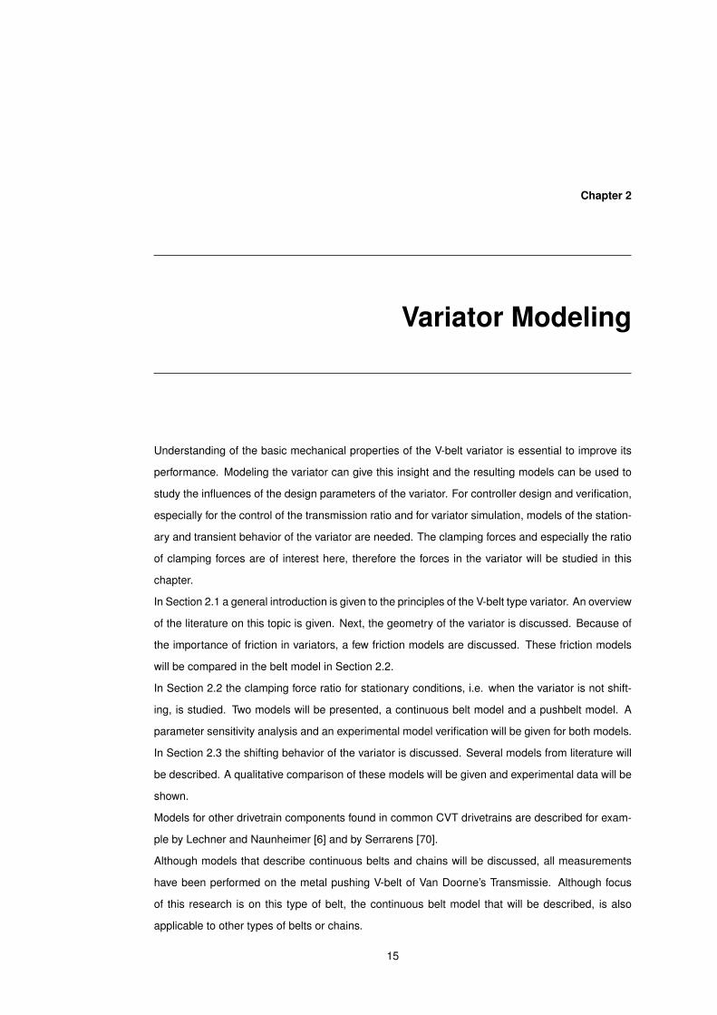
Friction models First, the effects of several friction models are compared. In Figure 2.8(a) Ψ is
shown for several friction models. From the figure can be seen that except for the viscous friction
model (the dashed line in this figure), the sensitivity of the value of Ψ for different friction models is
small. Comparing the normal force distribution calculated with the continuous belt model as shown
in Figure 2.8(b) shows the same result. The Coulomb friction model, the Visco-plastic model and
the continuous Stribeck model give comparable results for the value of Ψ. The viscous friction
model however does not compare well to the measured values as will be shown later.
The belt-tension is shown in Figure 2.8(c). The tension in the belt is a linear function of the normal
force distribution (See Equations (2.29) and (2.23)). The different behavior of the viscous friction
model can also be seen in the belt-tension and in the rate of change of the belt-tension along the
wrapped angle of the pulley. This is shown in Figure 2.8(d).
All friction models have been tuned to have comparable friction coefficients. It can be clearly seen
from the figure that viscous damping results in completely different behavior. This model gives very
different results than actually measured in variators (See Figure 2.12). The viscous damping model
is clearly not applicable for belt type variators.
Friction coefficient The influence of the friction coefficient using the Coulomb friction model can
be seen in Figure 2.9(a). From this figure can be seen that a higher value of the friction coefficient
influences Ψ in such a way that the highest value becomes higher and the lowest value becomes
lower. This is caused by the tension in the belt. If the friction coefficient becomes higher, the tension
difference in the belt also increases due to the fact that more torque can be transferred with the
clamping force remaining the same.
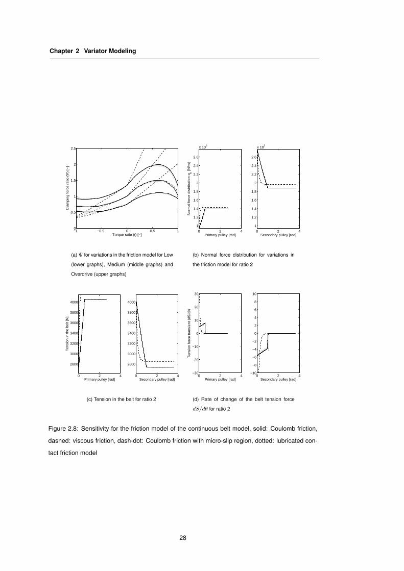
Parameter AE For parameter AE (the cross sectional area of the belt times Young’s modulus)
only the lubricated contact friction model is shown, because the Coulomb friction model has no
sensitivity for this parameter. This is due to the fact that the Coulomb friction model is not sensitive
to the speed of the sliding contact. The results are shown in Figures 2.10(a) and 2.10(b). Using
the visco-plastic friction model or the continuous Stribeck curve the Ψ will change with changes of
27
Chapter 2 Variator Modeling
−1 −0.5 0 0.5 10
0.5
1
1.5
2
2.5
Torque ratio (τ) [−]
Cla
mpi
ng fo
rce
ratio
(Ψ)
[−]
(a) Ψ for variations in the friction model for Low
(lower graphs), Medium (middle graphs) and
Overdrive (upper graphs)
0 2 4
1
1.2
1.4
1.6
1.8
2
2.2
2.4
2.6
x 105
Primary pulley [rad]
Nor
mal
forc
e di
strib
utio
n q n [N
/m]
0 2 4
1
1.2
1.4
1.6
1.8
2
2.2
2.4
2.6
x 105
Secondary pulley [rad]
(b) Normal force distribution for variations in
the friction model for ratio 2
0 2 4
2800
3000
3200
3400
3600
3800
4000
Primary pulley [rad]
Ten
sion
in th
e be
lt [N
]
0 2 4
2800
3000
3200
3400
3600
3800
4000
Secondary pulley [rad]
(c) Tension in the belt for ratio 2
0 2 4−30
−20
−10
0
10
20
30
Primary pulley [rad]
Ten
sion
forc
e tr
ansi
ent (
dS/d
θ)
0 2 4−10
−8
−6
−4
−2
0
2
4
6
8
10
Secondary pulley [rad]
(d) Rate of change of the belt tension force
dS/dθ for ratio 2
Figure 2.8: Sensitivity for the friction model of the continuous belt model, solid: Coulomb friction,
dashed: viscous friction, dash-dot: Coulomb friction with micro-slip region, dotted: lubricated con-
tact friction model
28

2.2 Stationary Variator Modeling
−1 −0.5 0 0.5 10
0.5
1
1.5
2
2.5
Torque ratio (τ) [−]
Cla
mpi
ng fo
rce
ratio
(Ψ)
[−]
(a) Ψ for variations in friction coefficient for Low
(lower graphs), Medium (middle graphs) and
Overdrive (upper graphs)
0 2 41
1.2
1.4
1.6
1.8
2
2.2
2.4
2.6
x 105
Primary pulley [rad]
Nor
mal
forc
e di
strib
utio
n q n [N
/m]
0 2 41
1.2
1.4
1.6
1.8
2
2.2
2.4
2.6
x 105
Secondary pulley [rad]
(b) Normal force distribution for variations in
friction coefficient
0 2 4
2800
3000
3200
3400
3600
3800
4000
Primary pulley [rad]
Ten
sion
in th
e be
lt [N
]
0 2 4
2800
3000
3200
3400
3600
3800
4000
Secondary pulley [rad]
(c) Tension in the belt for ratio 2
0 2 4−30
−20
−10
0
10
20
30
Primary pulley [rad]
Ten
sion
forc
e tr
ansi
ent (
dS/d
θ)
0 2 4−30
−20
−10
0
10
20
30
Secondary pulley [rad]
(d) Rate of change of the belt tension force
dS/dθ for ratio 2
Figure 2.9: Sensitivity for friction coefficient of the continuous belt model shown for the visco-plastic
friction model, solid: μ = 0.08, dashed: μ = 0.09, dash-dot: μ = 0.10, dotted: μ = 0.11.
29
Chapter 2 Variator Modeling
−1 −0.5 0 0.5 10
0.5
1
1.5
2
2.5
Torque ratio (τ) [−]
Cla
mpi
ng fo
rce
ratio
(Ψ)
[−]
(a) Ψ for variations in stiffness for Low (lower
graphs), Medium (middle graphs) and Over-
drive (upper graphs)
0 2 4
1
1.2
1.4
1.6
1.8
2
2.2
2.4
2.6
2.8
3x 10
5
Primary pulley [rad]
Nor
mal
forc
e di
strib
utio
n q n [N
/m]
0 2 4
1
1.2
1.4
1.6
1.8
2
2.2
2.4
2.6
2.8
3x 10
5
Secondary pulley [rad]
(b) Normal force distribution for variations in
stiffness
Figure 2.10: Sensitivity for stiffness of the continuous belt model
AE. If AE is high, the belt will slide along a larger portion of the pulley, because the sliding speed
will remain small and therefore the friction coefficient will also remain small. If AE is lowered, the
friction coefficient will increase until AE is low enough for full sliding friction to occur in some portion
of the wrapped angle, while another part is still idle. If this happens, then the friction coefficient will
decrease again with decreasing AE.
Slip angle Although the running radius is assumed constant in this model (zero pulley deforma-
tion) the effect of the radial friction can be approximated using γ, the belt-slip angle. If γ is taken
constant over the whole wrapped angle of the belt on the pulley, the results for different values of
γ are given in 2.11(a) and 2.11(b). The assumption of a constant value for γ is further evaluated
in the section on the effects of pulley deformation. This way of tuning γ to fit the data implicitly
assumes that the running radius on the pulley is continuously in- or decreasing. This is the case
for spiral running.
Optimized parameters If the calculated Ψ is set against measured data, the difference can be
quite large as can be seen in Figure 2.12(a). The initial value γ = 0 is apparently not very accu-
rate. Therefore both the values of γ and μ are used to fit the model more accurately to the data.
The friction model used is the Coulomb friction model, because the sensitivity of the model to the
friction model is not very high. Using the Coulomb friction model also the parameter AE is not
important for the parameter fit. The result is shown in Figure 2.12(b). The model is fitted more
closely to the positive torque values, because this is the area in which the variator will operate in
more frequently in automotive applications. The model matches the data more closely with the
optimized values. The optimized values are:
30

2.2 Stationary Variator Modeling
−1 −0.5 0 0.5 10
0.5
1
1.5
2
2.5
Torque ratio (τ) [−]
Cla
mpi
ng fo
rce
ratio
(Ψ)
[−]
(a) Ψ for variations in γ for Low (lower graphs),
Medium (middle graphs) and Overdrive (upper
graphs)
0 2 41
1.5
2
2.5
3
3.5
4
x 105
Primary pulley [rad]
Nor
mal
forc
e di
strib
utio
n q n [N
/m]
0 2 41
1.5
2
2.5
3
3.5
4
x 105
Secondary pulley [rad]
(b) Normal force distribution for variations in γ
Figure 2.11: Sensitivity for γ of the continuous belt model
Parameter Value
μ 0.1 [-]
γ 0.8 [rad]
The high value of γ that is needed to accurately track the measured values of Ψ is probably due to
omission of the bands-blocks interaction in this model. This value is therefore not representative of
a ’real’ spiral running, but rather the compensation for the omission of some physical properties in
the model.
Conclusions continuous belt model
From the results in this section follows that the continuous belt model can be very accurate for pos-
itive values of Tp, although the model does not take compression forces into account. The value
Ψ which is an important property for ratio control, as will be shown later in Section 2.3, can be
accurately simulated using the continuous belt model.
The friction model that is used in the calculation does not have a large influence on the calculated
result, except for the viscous friction model. The viscous friction model apparently does not accu-
rately describe the friction in the variator. Coulomb friction describes the variator friction in sufficient
detail, therefore this model is used in simulations.
Furthermore, the stiffness of the belt is of little consequence to the belt tension distribution. The
spiral running however, is an important factor in the calculation of the belt tension. This can be seen
in the sensitivity to the angle γ, the slip angle of the belt on the pulley. Also the friction coefficient
is an important factor.
31

Chapter 2 Variator Modeling
−1 −0.5 0 0.5 10
0.5
1
1.5
2
2.5
Torque ratio (τ) [−]
Cla
mpi
ng fo
rce
ratio
(Ψ)
[−]
(a) Calculated with γ = 0
−1 −0.5 0 0.5 10
0.5
1
1.5
2
2.5
Torque ratio (τ) [−]
Cla
mpi
ng fo
rce
ratio
(Ψ)
[−]
(b) Calculated with optimized γ and μ
Figure 2.12: The calculated Ψ (solid) versus the measured data (dashed) for Low (lower graphs),
Medium (middle graphs) and Overdrive (upper graphs)
32

2.2 Stationary Variator Modeling
2.2.2. Pushbelt model
The metal pushbelt as produced by Van Doorne’s Transmissie has some special properties not
captured by the continuous belt model. The pushbelt consists of blocks and bands as discussed
earlier. The blocks can move freely along the bands. Between the blocks a small gap exists de-
pending on the tension force in the bands.
Numerous works have been contributed to the modeling of the metal pushing V-belt variator. Ger-
bert [31] assumes the tension in the belt to be constant, because the stiffness of the bands is lower
than the stiffness of the blocks. Also Kim [42] assumes the tension in the bands to be constant, but
he assumes the friction between bands and blocks to be negligible. Others like Sun [82] assume
the friction to be small with a value of around 0.01. In this section the following assumptions are
made:
• the bands are assumed to be a continuous belt with negligible bending stiffness,
• friction exists between bands and blocks, therefore the tension in the bands will not be con-
stant,
• in the belt there is always one part where compression is zero, this means that there is some
play between the blocks in the belt,
• the compression force between the blocks can not be higher than the tension in the bands at
any point in the pushbelt, the pushbelt would otherwise buckle,
• inertia forces can be neglected, the centrifugal forces are not taken into account,
• the friction coefficients are constant (Coulomb friction model), the Stribeck effect is not taken
into account.
In a pushbelt the bands are packed tightly together, forming a belt. This belt has a very low bending
stiffness due to the fact that the individual bands are very thin. Therefore, the bending stiffness can
be neglected. Also, because of the tight packaging, the belt can be viewed to be continuous. In
reality the bands move relative to each other as well, but this effect is neglected here.
The blocks and the bands are not fixed, i.e. they can move relative to each other. The con-
tact surface is lubricated, lowering the friction, but high normal forces make this friction relevant.
Furthermore, it is assumed that there is a (small) amount of play between the blocks in the belt.
Therefore, there must be a point in the belt where the compression between the blocks is zero,
since there is a gap between the blocks.
If the compression force between the blocks would be higher than the tensile force in the belt. If
this was the case, a net compression force would result. The result of this would be buckling of the
belt, due to the lack of bending stiffness in the belt.
The inertial forces are neglected here. In reality these forces are present and can be relevant for
33

Chapter 2 Variator Modeling
S S+dS
Fd
μ1Fd
(a) Side view forces on bands
Fd
μ1Fd
Q+dQQ
sin( )Fnβ
μ2Fn γ
(b) Side view forces on blocks
FnFn
Fd
β
(c) Front view forces on blocks
Figure 2.13: Forces acting on the belt according to the pushbelt model
high speed operation of the variator. For the comparison between the models and the model pa-
rameter sensitivity study the inertial forces are not of interest.
Because of the very small influence of the friction model on the outcome of the continuous belt
model, only the Coulomb friction model is used in this section.
2.2.3. Forces in the pushbelt
Forces acting on the bands and blocks of a metal V-belt are shown in Figure 2.13. The blocks now
form a layer between the belt and the pulley. There can be no tension between the blocks, but they
can transmit torque when compressed, hence the name pushbelt. Because there is no pre-strain
in the belt, there is some play between the blocks when not compressed. This is necessary for the
belt to be able to bend.
The forces acting on the blocks and the bands have to be in equilibrium in stationary conditions:
dQ = 2μ2 cos γdFn − μ1dFd (2.37)
dS = −μ1dFd (2.38)
dFd = dθS (2.39)
dFd = dθQ + 2 sinβdFn + 2 sin γμ2dFn (2.40)
The equilibrium Equations (2.37), (2.38), (2.39) and (2.40) can be combined to a set of differential
equations given in 2.41 through 2.43.
dS
dθ= −μ1S (2.41)
34

2.2 Stationary Variator Modeling
dQ
dθ= − μ2 cos γ
2 (sinβ + μ2 sin γ)Q +
[μ2 cos γ
2 (sinβ + μ2 sin γ)− μ1
]S (2.42)
dFn
dθ=
S − Q
2 (sinβ + μ2 sin γ)(2.43)
In line with many publications a Coulomb friction model is assumed here. This gives the possibility
to find an analytical solution to the differential equations. The solution then still depends on the
boundary conditions. Integrating Equation (2.41)-(2.43) gives:
S = S0e−μ1θ (2.44)
Q = Q0e− μ2 cos γθ
2(sin β+μ2 sin γ) +∫ ([
μ2 cos γ
2 (sinβ + μ2 sin γ)− μ1
]S
)dθ (2.45)
Q = Q0e− μ2 cos γθ
2(sin β+μ2 sin γ) +[
μ2 cos γ
2μ1 (sin β + μ2 sin γ)− 1
]S0
[e−μ1θ − 1
](2.46)
In the more general form the differential equations can be used to find a numerical solution.
Results
If the model described in the previous paragraph is used to calculate the forces in the belt numeri-
cally, then the boundary conditions need to be known. In the case of the pushbelt model there exist
four different regimes, shown in Figure 2.14, each having their own set of boundary conditions. The
four different regimes are:
• rg ≤ 1, Tp ≥ Rp (S1 − S0)
• rg ≤ 1, Tp < Rp (S1 − S0)
• rg > 1, Tp ≥ Rp (S1 − S0)
• rg > 1, Tp < Rp (S1 − S0)
To determine, for a given operating point of the variator, in which regime the variator is, it has to be
determined whether the bands slip on the blocks on the primary or on the secondary side. Sec-
ondly, it has to be determined on which side the compression is higher than zero. The direction of
the friction force between the bands and the blocks is determined by the speed difference between
the blocks and the bands. The speed difference depends on the transmission ratio.
In low, ratios lower than one, when the belt has a larger running radius on the secondary pulley, the
bands will slip on the primary side. Because the bands will run faster than the blocks, the tension
will decrease on the primary side, aiding the transmission of torque. The torque at which the com-
pression force changes sides will therefore be lower than zero. In ratios greater than one the bands
will slip on the secondary side. In contrast to the first situation, the bands will counteract the torque
transmission. The torque at which the compression side will change will therefore be greater than
zero.
35

Chapter 2 Variator Modeling
−0.1 −0.05 0 0.05 0.1 0.15 0.2
−0.1
−0.05
0
0.05
0.1
S
Q
(a) rg > 1, positive compression (Q0 > 0)
−0.1 −0.05 0 0.05 0.1 0.15 0.2
−0.1
−0.05
0
0.05
0.1
S
Q
(b) rg > 1, negative compression (Q1 ≥ 0)
−0.05 0 0.05 0.1 0.15 0.2 0.25
−0.1
−0.05
0
0.05
0.1
S
Q
(c) rg ≤ 1, positive compression (Q0 > 0)
−0.05 0 0.05 0.1 0.15 0.2 0.25
−0.1
−0.05
0
0.05
0.1
S
Q
(d) rg ≤ 1, negative compression (Q1 ≥ 0)
Figure 2.14: Tension and compression force distribution
36
2.2 Stationary Variator Modeling
The boundary conditions for the differential equations is given by the torque and its direction and
the transmission ratio.
Low In low ratio (rg < 1), where the belt runs at a smaller radius on the primary pulley and on
a larger radius on the secondary pulley, the bands will slip on the blocks on the primary pulley.
Because the relative difference between the running radius of the bands and the running radius
of the blocks is larger on the primary pulley than on the secondary pulley, the bands will move
slower than the blocks on the primary pulley. This effect causes a positive torque to be transmitted
when no compression force is present. The corresponding tension and compression force dis-
tribution are shown in Figure 2.14(c) and 2.14(d) for T > −T0 and T ≤ −T0 respectively, with
T0 = Rp(S1 − S0).
Overdrive In overdrive ratio (rg > 1) this situation occurs on the secondary pulley. This causes
a negative torque for the situation of no compression force. In medium ratio this effect does not
occur, because the difference between the bands and the blocks is zero on both sides (no slip oc-
curs). The corresponding tension and compression force distribution are shown in Figure 2.14(a)
and 2.14(b) for T ≥ T0 and T < T0 respectively.
Parameter sensitivity
The influence of model parameters on the calculation of the Ψ are determined for the pushbelt
model. For the parameter γ the results are shown in Figure 2.15. From this figure can be seen that
the Ψ is lowered with an increasing value of γ. For negative values of γ the value of Ψ increases.
In Figure 2.16 shows the parameter sensitivity for μ2. For an increasing value of μ2, the friction
coefficient between blocks and pulley, the value of Ψ increases for positive torque and decreases
for negative torque. The inverse is true for decreasing values of μ2.
The parameter sensitivity of the friction coefficient between blocks and bands, μ1, is shown in
Figure 2.17. Only slight change is observed for changes in μ1. For increasing values of μ1 the
ratios above medium (ratio> 1) show a decrease in Ψ and the results for low ratios (ratio< 1) show
an increase in the value of Ψ. In medium no change is seen.
Parameter sensitivity for the clamping force is zero as is shown in Figure 2.18. The torque in-
creases proportionally with the clamping force and therefore the resulting change in Ψ vs torque
ratio equals zero.
If the model is tuned to measured data, the model parameters are:
37

Chapter 2 Variator Modeling
−1 −0.5 0 0.5 10
0.5
1
1.5
2
2.5
3
Torque ratio (τ) [−]
Cla
mpi
ng fo
rce
ratio
(Ψ)
[−]
Figure 2.15: Ψ curve sensitivity for γ, solid: γ = 0, dashed: γ = 0.04 and dash-dot: γ = 0.08
(upper graph: rg = 2.25 (OD), middle graph: rg = 1 (MED) and lower graph: rg = 0.45 (LOW))
−1 −0.5 0 0.5 10
0.5
1
1.5
2
2.5
3
Torque ratio (τ) [−]
Cla
mpi
ng fo
rce
ratio
(Ψ)
[−]
Figure 2.16: Ψ curve sensitivity for μ2, with solid: μ2 = 0.09, dashed: μ2 = 0.08 and dash-dot:
μ2 = 0.11 (upper graph: rg = 2.25 (OD), middle graph: rg = 1 (MED) and lower graph: rg = 0.45
(LOW))
38
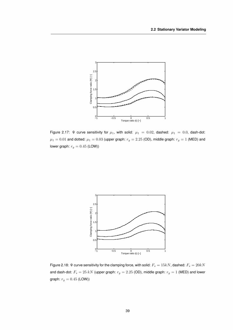
2.2 Stationary Variator Modeling
−1 −0.5 0 0.5 10
0.5
1
1.5
2
2.5
3
Torque ratio (τ) [−]
Cla
mpi
ng fo
rce
ratio
(Ψ)
[−]
Figure 2.17: Ψ curve sensitivity for μ1, with solid: μ1 = 0.02, dashed: μ1 = 0.0, dash-dot:
μ1 = 0.01 and dotted: μ1 = 0.03 (upper graph: rg = 2.25 (OD), middle graph: rg = 1 (MED) and
lower graph: rg = 0.45 (LOW))
−1 −0.5 0 0.5 10
0.5
1
1.5
2
2.5
3
Torque ratio (τ) [−]
Cla
mpi
ng fo
rce
ratio
(Ψ)
[−]
Figure 2.18: Ψ curve sensitivity for the clamping force, with solid: Fs = 15kN , dashed: Fs = 20kN
and dash-dot: Fs = 25 kN (upper graph: rg = 2.25 (OD), middle graph: rg = 1 (MED) and lower
graph: rg = 0.45 (LOW))
39

Chapter 2 Variator Modeling
−1 −0.5 0 0.5 10
0.5
1
1.5
2
2.5
Torque ratio (τ) [−]
Cla
mpi
ng fo
rce
ratio
(Ψ)
[−]
Figure 2.19: Ψ curve comparison with measured data (dashed curves) and calculated data (solid
curves). (upper graph: rg = 2.25 (OD), middle graph: rg = 1 (MED) and lower graph: rg = 0.45
(LOW))
Parameter Value
μ2 0.08
μ1 0.03
γ r = 0.5: 0.05, r = 1: 0.00, r = 2.5: 0.22
The value of μ1 and μ2 are not sensitive to the ratio. This finding is intuitive, because the tribological
circumstances are equal in all ratios. The same is not true for the value of γ. This value however is
very high in overdrive. Possibly some unmodeled effects are represented in this value. The result
is shown in Figure 2.19. For positive torque the model matches very closely to the measured data,
but for negative torque large differences can be seen.
2.2.4. Conclusion stationary model
The calculation of the clamping force ratio Ψ can be done with either the continuous belt model or
the pushbelt model. Although the pushbelt model is more complex and takes the complex kinemat-
ics of the pushbelt into account, the results are not more accurate when compared to measured
data.
For calculating the clamping force ratio for a pushbelt variator it is sufficient to use the continu-
ous belt model. However, the continuous belt model does not take into account the discontinuous
behavior of the pushbelt that occurs when the regime of the variator changes, i.e. when the com-
pression side changes or the ratio changes through rg = 1. If this behavior needs to be simulated,
then the pushbelt model must be used.
40
2.3 Variator Transient Model
2.3. Variator Transient Model
The transient behavior of a V-belt type variator, i.e. the shifting behavior, is discussed in this section.
To shift a V-belt type variator either a creeping process caused by elastic deformations of pulley and
belt or a sliding process has to occur. The shifting by elastic deformation is commonly referred to
as creep-mode shifting. The sliding process is called slip-mode shifting. Therefore we define two
types of slip:
Definition 7 When stable, creep like, slipping occurs, i.e. the friction coefficient increases with
increasing slip, it is said that micro-slip occurs.
Definition 8 When unstable slipping occurs, i.e. the friction coefficient decreases with increasing
slip, it is said that macro-slip occurs.
2.3.1. Creep-mode shifting
Creep-mode shifting is the main shift mode for pushbelt type variators. This shiftmode is charac-
terized by the way the variator changes ratio. In creep-mode shifting the ratio change is caused by
elastic deformation of the belt and pulleys. No macro-slip occurs. This type of shifting is modeled
by several authors. Ide [36] developed a model for creep mode shifting that states that shifting
is proportional to the input speed and the difference between the primary clamping force and the
primary clamping force needed for equilibrium. Shafai [71] however suggests that the shifting pro-
cess can be described as a moving mass with viscous damping. Several authors suggest that the
shifting behavior of the CVT is linked to deformation of belt and pulleys [18] [17] [79].
In creep mode shiftspeed is dependent on the actuation forces, rotating speed of the pulleys and
pulley and belt deformation. Pulley and belt deformation is the means by which shifting is possible.
More flexible pulleys give faster shifting. Pulley deformation is also dependent on the running radius
of the belt on the pulley.
If the variator is symmetrical, upshifting should be the opposite of downshifting. Because the stiff-
ness of the pulley-belt system is dependent on the ratio of the variator, a ratio dependence can be
expected in the ratio changing behavior. Furthermore a clamping force dependency follows from
the increased deformation of the pulleys and the belt with a higher clamping force. Finally, with
higher rotational speed faster ratio changing can be observed.
2.3.2. Slip-mode shifting
Slip-mode shifting is the characterization of the ratio changing behavior of a variator when macro-
slip is occurring. This type of shifting is much faster than creep-mode shifting, because the sliding
motion of the belt on the pulley reduces the friction in radial direction and the primary and sec-
ondary speeds are completely decoupled, i.e. the primary and secondary inertias do not have to
be accelerated.
41

Chapter 2 Variator Modeling
While shifting when slipping is very fast, ratio changing which causes slip to increase instead of
decrease can cause serious damage to the variator since the absorbed energy in the pulley-belt
contact will increase.
In slip-mode, shifting is not limited by the elastic deformations in the belt and/or pulley. Slip-mode
shifting is therefore not dependent on the rotational speed of the variator and the speed of shifting
is limited only by the actuation system. Ide has studied this type of shifting behavior of a pushbelt
type variator [37].
2.3.3. Models
Over time several models have been proposed to describe the transient behavior of a V-belt type
variator. A short overview of often used models is given. Also an analysis using dimensional
analysis of the shifting behavior is given based on the work of Carbone in [17].
Dimensional Analysis
The rate of change of the ratio rg is expressed as a function of: the clamping forces Fp and Fs,
the input and output torques Tp and Ts, the primary and secondary running radii Rp and Rs, the
length of the belt, the axial pulley distance, the primary and secondary shaft speeds, pulley and
belt stiffnesses kp and ks, beltspeed and the pulley groove angle. This can be written as:
rg = f (Fp, Fs, Tp, Ts, Rp, Rs, L, a, ωp, ωs, kp, ks, vb, β) (2.47)
This function can be rewritten to a dimensionless form using as fundamental units the quantities
Rp, Fs and ωp using Buckingham’s pi-theorem [14] [16] [15]. Equation (2.47) now can be written
as:rg
ωp= F
(Fp
Fs,
Tp
FsRp,
Ts
FsRp,Rs
Rp,
L
Rp,
a
Rp,ωs
ωp,kpRp
Fs,ksRp
Fs,
vbelt
Rpωp, β
)(2.48)
This equation can be further simplified by using the fact that β, L and a are constants and that
ωs/ωp = rs, Tp/(FsRp) = cτ , Tp/Ts = rg and Rp/Rs = rg. Furthermore, if kp and ks are
approximately equal ks can be omitted. This is the case if the pulley stiffness is (nearly) equal
of both pulleys. This will be the case if the variator is symmetrical. Equation (2.48) can then be
rewritten as:rg
ωp= F
(Fp
Fs, τ, rg, rs,
kpRp
Fs,
vbelt
Rpωp
)(2.49)
For creepmode shifting, where no macro-slip occurs, the following assumptions can be made:
vb/(Rpωp) ≈ 1 and rs ≈ rg. The shifting process therefore has to be a function of the input shaft
speed, the clamping force ratio, the torque ratio, the transmission ratio and a factor determined by
the pulley stiffness.
Ide
Ide found that the shiftspeed of the variator is a function of the speed ratio rs and is linearly de-
pendent on the input speed [36]. He also found a linear relationship with the difference between
42

2.3 Variator Transient Model
the primary clamping force and the primary clamping force for which the variator does not shift.
Furthermore he found that this shiftspeed further depended on the ratio of the variator.
The resulting model is:
rg = ωpκide(rg)Fs
(Fp
Fs− Ψ
)(2.50)
In this equation κide(rg) is a function of rg, which must be obtained using experimental data.
Shafai
Shafai models the variator as being a damped single mass system [71]:
mrxp + crxp = Fs
(Fp
Fs− Ψ
)(2.51)
The acceleration term is very small compared to the damping term, therefore the acceleration
terms may be neglected (|mrxp| << |crxp|). If the acceleration term is neglected the following
differential equation remains:
xp =1cr
Fs
(Fp
Fs− Ψ
)(2.52)
In this equation cr is a damping coefficient, which must be determined using experimental data.
If this equation is rewritten in terms of the geometric ratio rg substitution of the time derivative of
Equation (2.3) for xp, the following results:
rg =1 − rg
crRs tanβFs
(Fp
Fs− Ψ
)(2.53)
CMM
The Carbone Mangialardi Mantriota (CMM) model was introduced recently. Carbone [17] reasons
that the shiftspeed of the variator must be almost linear with the logarithm of the clamping force
quotient Fp/Fs. Not only did this give a better approximation of the results they had from other,
more complex models, but the reasoning that the shifting process must be symmetric around rs = 1
gives rise to this suggestion.
According to the CMM model, the transient behavior of a V-belt type variator can be described by:
rg = κcmm(rg, [Fs])ωp
(ln
Fp
Fs− ln Ψ
)(2.54)
In this equation κcmm(rg, [Fs]) is a function of rg and for higher accuracy also Fs, which can be
obtained from experiments or from theory.
2.3.4. Measurements
Measurements have been done to validate or invalidate the models mentioned in the previous
paragraph. These measurements have been done on a beltbox testrig. These measurements will
be compared with the given models and the results will be compared.
43

Chapter 2 Variator Modeling
Analysis
In Figure 2.20(a) measurements are shown of rg against the clamping force ratio Fp/Fs. In this
figure can be seen that indeed for low shiftspeeds rg is more or less linear with Fp/Fs. However,
for higher shifting speeds, especially for lower ratio’s a clear deviation from Ide’s transient behavior
theory is present. If these results are compared to the results shown in Figure 2.20(b), then it can
be seen that increasing the clamping force increases the shiftspeed. The relation however is not
linear. With a doubling of the clamping force the shiftspeed increases much less than a factor two.
In Figure 2.20(c) the results are shown from measurements with a doubled input shaft speed. If
these results are compared to the results from Figure 2.20(a), then it can be seen that doubling the
input shaft speed also doubles the shiftspeed. If these measurements are compared to the models
shown earlier, then it can be seen that the model from Shafai does not take into account the
dependency on the input shaft speed and assumes a linear relation with the secondary clamping
force. Both can be seen to be untrue.
For the model presented by Ide follows that the input shaft speed is taken into account in a linear
way as follows from the measurements. The clamping force however is also present in a linear
fashion in the Ide model. This does not compare well to the measurements.
For the CMM model, the results should be compared to the logarithm of the clamping force ratio.
These results are shown in Figure 2.21. These are the same measurements as shown earlier in
a logarithmic scale. As can be seen in this figure, the logarithm of the clamping force ratio gives
an almost linear relation to the shiftspeed. Furthermore, the clamping force is not a factor in the
CMM model. In the CMM model however, there is a constant factor for the pulley deformation. If
this factor is related to the clamping force, the CMM model can very accurately describe the rate
of change of speed ratio. In Figure 2.21(a), 2.21(b) and 2.21(c) the model results from the CMM
model are compared to the measured values of rg. In these graphs the clamping force effect on
shiftspeed is taken into account in the CMM model.
44
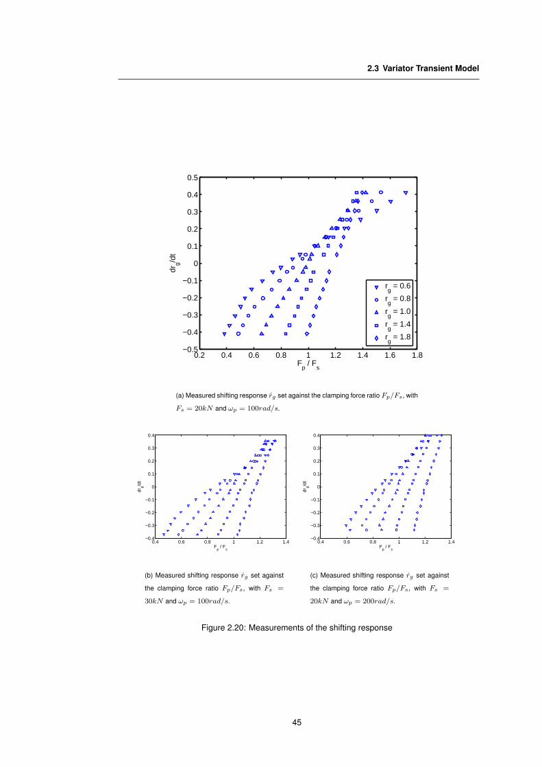
2.3 Variator Transient Model
0.2 0.4 0.6 0.8 1 1.2 1.4 1.6 1.8−0.5
−0.4
−0.3
−0.2
−0.1
0
0.1
0.2
0.3
0.4
0.5
Fp / F
s
drg/d
t
rg = 0.6
rg = 0.8
rg = 1.0
rg = 1.4
rg = 1.8
(a) Measured shifting response rg set against the clamping force ratio Fp/Fs, with
Fs = 20kN and ωp = 100rad/s.
0.4 0.6 0.8 1 1.2 1.4−0.4
−0.3
−0.2
−0.1
0
0.1
0.2
0.3
0.4
Fp / F
s
drg/d
t
(b) Measured shifting response rg set against
the clamping force ratio Fp/Fs, with Fs =
30kN and ωp = 100rad/s.
0.4 0.6 0.8 1 1.2 1.4−0.4
−0.3
−0.2
−0.1
0
0.1
0.2
0.3
0.4
Fp / F
s
drg/d
t
(c) Measured shifting response rg set against
the clamping force ratio Fp/Fs, with Fs =
20kN and ωp = 200rad/s.
Figure 2.20: Measurements of the shifting response
45

Chapter 2 Variator Modeling
−0.8 −0.6 −0.4 −0.2 0 0.2 0.4 0.6 0.8−0.5
−0.4
−0.3
−0.2
−0.1
0
0.1
0.2
0.3
0.4
0.5
ln (Fp / F
s)
drg/d
t
rg = 0.6
rg = 0.8
rg = 1.0
rg = 1.4
rg = 1.8
(a) Measured shifting response rg set against the clamping force ratio ln(Fp/Fs),
with Fs = 20kN and ωp = 100rad/s.
−0.8 −0.2 0.4−0.5
−0.4
−0.3
−0.2
−0.1
0
0.1
0.2
0.3
0.4
0.5
ln (Fp / F
s)
drg/d
t
(b) Measured shifting response rg set against
the clamping force ratio ln(Fp/Fs), with Fs =
30kN and ωp = 100rad/s.
−0.8 −0.2 0.4−0.5
−0.4
−0.3
−0.2
−0.1
0
0.1
0.2
0.3
0.4
0.5
ln (Fp / F
s)
drg/d
t
(c) Measured shifting response rg set against
the clamping force ratio ln(Fp/Fs), with Fs =
20kN and ωp = 200rad/s.
Figure 2.21: Measurements of the shifting response
46

2.3 Variator Transient Model
2.3.5. Comparison
If the CMM model is compared to both the Ide model and the model from Shafai, the difference can
be illustrated with the Taylor expansion of ln(Fp/Fs) − ln(Ψ):
lnFp
Fs− ln Ψ =
1Ψ
[Fp
Fs− Ψ
]− 1
21
Ψ2
[Fp
Fs− Ψ
]2
+ . . . (2.55)
Looking at this Taylor expansion can be seen that the Ide model and the Shafai model are a first
order approximation of the logarithm of the clamping force ratio used in the CMM model. Also it
can be seen that for values of Ψ smaller than one the difference can become large. From the mea-
surements indeed the large differences can be found for low ratios were the value of Ψ is smaller.
With the overstated influence of the clamping force in both Ide’s and Shafai’s model, it must be
concluded that overall the CMM model gives the most accurate results compared to our measure-
ments.
47

Chapter 2 Variator Modeling
48

Chapter 3
Slip in the variator
Slip in the variator is important for several reasons. First, slip can cause serious damage to the
belt and the pulleys. For this reason it is important to know the conditions that lead to the situations
where damage occurs. Second, to optimize the performance of the variator, both to maximize the
torque capacity and to minimize the clamping force, detailed information on the dynamics of slip
and the relation between slip and traction is necessary. Why slip is especially valuable for efficiency
optimization of the variator will become apparent in the next chapter, on variator efficiency.
Models for the slipping behavior of the variator are studied by Klaassen [44] and Bonsen [11],
proposing a dynamical model for slip in a CVT. Kim [42], [10] and Asayama [5] propose a model
for the traction behavior of a pushbelt type variator. Van Drogen and van der Laan [89] study the
relation between slip and damage in the variator experimentally.
In this chapter slip in the variator is studied. First, the relation between slip and traction is discussed,
using a kinematical pushbelt model. Measurements of the traction in a pushbelt variator will be
shown.
Second, a dynamic model to describe slip in the variator is derived. The dynamics of slip are
important when designing a slip control system. Furthermore, the model is used to determine the
stability criteria for the pushbelt variator.
Third, several slip estimation methods will be discussed. Correct estimation of the slip in a variator
is essential to be able to use the variator at its full capability, since its characteristics are closely
related to this variable.
3.1. Slip and Traction
The V-belt type variator utilizes friction to transmit power from the driving pulley to the belt and from
the belt to the driven pulley. In this chapter it is assumed that the primary pulley is the driving pulley.
The effective friction coefficient, i.e. the average friction coefficient, along the wrapped arc of the
belt on the pulley is called traction.
49

Chapter 3 Slip in the variator
Definition 9 The dimensionless traction coefficient μeff is defined here by:
μeff =Ts cos β
2 min(Fs, Fp)Rs=
Tp cos β
2 min(Fs, Fp)Rp(3.1)
where Tp and Ts are the torque on the primary and secondary shaft of the variator, β is the pulley
angle, Fp and Fs are the primary and secondary clamping forces and Rp and Rs are the running
radii of the belt on the pulley on the primary and secondary side respectively. Ts/Rs = Tp/Rp,
because the forces acting on the belt on either pulley must be equal.
The traction coefficient μeff is also referred to as simply μ.
In this definition μeff is the transmitted output torque divided by the contact normal force between
the belt and the pulley with the lowest clamping force. According to the models presented in Chap-
ter 2, the pulley with the smallest wrapped angle will also have the smallest clamping force when
traction is maximal.
Measurements show [25] that the traction coefficient depends on the (micro-)slip between the belt
and the pulleys. Since the traction coefficient defined according to 3.1 is a global variable, a global
measure for the slip is required to characterize the relation between slip and traction. A possible
global measure for the slip is the so-called speed loss vs in the variator, defined by:
vs = ωpRp − ωsRs (3.2)
Later in this section it will be shown that the traction does depend only weakly on the input speed
ωpRp. Therefore a relative slip is defined as the speed loss divided by the input speed ωpRp.
Definition 10 Relative slip is a dimensionless variable describing the relative motion between the
pulleys and the belt.
ν =vs
ωpRp= 1 − ωsRs
ωpRp= 1 − rs
rg(3.3)
Several authors have used this definition of slip [47] [10] [94] [89]. In the sequel, the term slip means
relative slip, unless stated otherwise. Besides, the term traction is often used as an abbreviation for
traction coefficient.
3.1.1. Traction curve
The traction curve is a diagram of the relation between slip (3.3) and traction (3.1). In Figure 3.1
measured traction curves of a typical variator are shown for three different ratios. The notable
differences between the traction curves will be discussed in Paragraph 3.1.2.
As can be seen in Figures 3.1, 3.2 and 3.3, traction is zero at zero slip. For increasing values of the
slip, the traction increases until a certain maximum value is reached and then is constant or slightly
decreasing. For small values of slip the traction is nearly linear with slip. This part of the curve with
viscous behavior, is called the micro-slip area. For larger values of slip, when traction decreases
50
3.1 Slip and Traction
with increased slip, it is said that the variator operates in the macro-slip area.
Figure 3.2 shows three traction curves for different input speeds. The traction curves are almost
identical in the micro-slip area. In the macro-slip area, there are distinct differences. Speed has
no influence in the micro-slip area, because the slip velocity is very small and the amount of slip is
determined predominantly by the wrapped angle. In macro-slip, the friction coefficient decreases
with increasing slipspeeds, causing a lower traction coefficient. This is caused by the Stribeck effect
[80].
In Figure 3.3 the traction curve is shown for different clamping forces. The micro-slip region slightly
moves to the right. As will be shown in paragraph 3.1.2 this is caused by the lengthening of the belt
and other elastic deformations under the higher load.
3.1.2. Play in the belt
It is assumed that all deformations of blocks and pulleys can be neglected. Furthermore, it is
assumed that rg < 1, so that Rp < Rs. Then, if slip occurs, this must occur at the primary pulley
(See Chapter 2). Let δt be the total play between the blocks in the belt, let the primary pulley be
the driving pulley and let the compression between the blocks have a positive contribution to the
transfer of power from the primary to the secondary pulley.
The speed of the blocks at the exit of the primary pulley is denoted by ve. This speed is constant
between the primary and secondary pulley, on the secondary pulley and between the secondary
and primary pulley. Because there is no slip between the secondary pulley and the belt, it follows
that ve = Rsωs. From the secondary pulley to the primary pulley and in the inactive arc on the
primary pulley there is no compression between the blocks. Obviously, play between the blocks
can only occur in this part of the belt. Here it is assumed that the total play in the belt is distributed
evenly between the blocks in the inactive part of the belt on the primary pulley (see Figure 3.5).
Experiments by Kobayashi [47] confirm this assumption.
The total gap between the block elements in the belt, δt, can be estimated by adding an initial gap
δo to the increase in belt length (ΔL) due to the internal stresses in the bands:
δt = δo + ΔL (3.4)
Hence, the mean gap δm is given by:
δm =δtde
αpRp(3.5)
where de is the thickness of a block and αp is the extend of the primary inactive arc.
The speed at which the blocks enter the pulley is ωpRp. Because the primary pulley is the driving
pulley ωpRp > ve. Therefore, the mean gap δm will be:
δm = (ωpRp − ve)T (3.6)
51

Chapter 3 Slip in the variator
0 1 2 3 4 5 60
0.02
0.04
0.06
0.08
0.1
0.12
ν [%]
μ [−
]
LowMedium
Overdrive
Figure 3.1: Traction as a function of slip measured at low, medium and overdrive (rg = 0.45 (solid),
rg = 1 (dash-dot) and rg = 2.25 (dashed))
0 1 2 3 4 5 60
0.02
0.04
0.06
0.08
0.1
0.12
ν [%]
μ [−
]
150 [rad/s]
225 [rad/s]
300 [rad/s]
Figure 3.2: Traction as a function of slip measured at overdrive for different input speeds ωp
(150 rad/s (solid), 225 rad/s (dashed) and 300 rad/s(dash-dot))
0 1 2 3 4 5 60
0.02
0.04
0.06
0.08
0.1
0.12
ν [%]
μ [−
]
5 [bar]8 [bar]
Figure 3.3: Traction as a function of slip measured at overdrive ratio for different clamping forces
(5 bar ∼ 5 kN (dashed) and 8 bar ∼ 8 kN (solid))
52

3.1 Slip and Traction
ve
ve
ωsωp
RsRp
Ts
Tp
αp
Figure 3.4: Pushbelt variator kinematics
δm
de
vp
v2
v1
Figure 3.5: Gaps in the belt
53

Chapter 3 Slip in the variator
0 1 2 3 4 5 60
0.01
0.02
0.03
0.04
0.05
0.06
0.07
0.08
0.09
Slip [%]
μ [−
]
Figure 3.6: Traction curves with increased gap (1.8 mm), (solid: model and dots: measured data )
Here T is the time that passes between the entry of two sequential blocks. Using ve = ωsRs and
Equation (3.3) it follows that:
ν =δt
αpRp(3.7)
The inactive arc should always contain at least one block element, otherwise (macro-)slip will occur.
It must be concluded that the presence of a gap δt must result in slip relative to the active arc on
the driving pulley. Furthermore, the decrease of the friction coefficient with increasing slip speed
has to be taken into account as shown by Kobayashi [47]. For this purpose the Stribeck friction
model may be used [58].
With Equation (3.7) slip and traction can be determined from measured data as will be shown in
Section 3.3. The tension and compression force distribution needed to calculate the lengthening of
the belt are found using the continuous belt model or the pushbelt model described in Chapter 2.
Also, we can calculate the idle arc from this model. From the idle arc, the length of the belt and the
initial gap we can calculate an estimate for slip in the belt for a given load.
In Figure 3.6 a comparison is shown for the calculated traction curve and measured data. The
measured data is acquired with an adapted belt. This belt had an increased gap, with one block
element of thickness de = 1.8mm removed. The influence of play is quite obvious. The point where
the slope of the traction curve changes, nearly discontinuously, coincides with the point where the
compression part changes to the other side. In the other traction curves this discontinuity is very
small, but can be seen in Figure 3.1 for low. For overdrive this discontinuity occurs for reversed
torque.
3.1.3. Results
The traction curve can be accurately described for micro-slip using this model. Measurements
shown in Figure 3.6 show that for a situation where the gap is enlarged by removing a block, the
model still accurately describes the traction curve.
54

3.2 Dynamic Variator Slip Model
3.2. Dynamic Variator Slip Model
The dynamics of slip as defined in Definition 10 is of interest for the design of a control system with
slip as the design variable. First a nonlinear model will be derived for the dynamics of the variator.
Then this model will be converted to a nonlinear model for slip in the variator. Finally a linearization
of this model is given, which will be the input for the control design process.
Slip is a function of four variables: ωp, ωs, Rp and Rs. With Rp and Rs mutually dependent by
the geometric configuration given by Equation (2.1), the geometric ratio is used as the dynamic
variable as defined in Definition 1.
The variator consists of two shafts each with one rotational degree of freedom and a variable
transmission ratio, which also introduces one degree of freedom. All other parts of the transmission,
engine or driveline are modeled as a varying input torque and a varying output torque.
Figure 3.7 gives a schematic representation of the test setup, which consists of a driving motor,
a variator and a load motor. The dynamical behavior of this system can be described by three
Je
Js
Te
ωp
ωs
Td
Fp
Fs
rg
Figure 3.7: Scheme of the test setup
differential equations, i.e. one for the primary side (with moment of inertia Je and driving torque
Te), one for the secondary side (with moment of inertia Js and load torque Td) and one for the
variator. In Figure 3.8 the free body diagrams of the primary and secondary side are shown. The
equations of motion for these part are given by:
Jeωp = Te − Tp − Tp,loss (3.8)
Jsωs = Ts − Ts,loss − Td (3.9)
where Tp and Ts are the torques, exerted by the belt on the primary and secondary pulley whereas
Tp,loss and Ts,loss are the loss torques at the primary and secondary side. These loss torques are
due to, amongst others, friction in the bearings of the shafts. It is assumed here that they are small
enough to neglect them. Rewriting of Equation (3.1) results in:
Tp =2
cos(β)μeff min(Fp, Fs)Rp(rg) (3.10)
for the primary torque Tp. If all inertia effects of the belt are neglected then, as shown in Chapter
2, the primary and the secondary torque are related by Ts = rgTp.
55
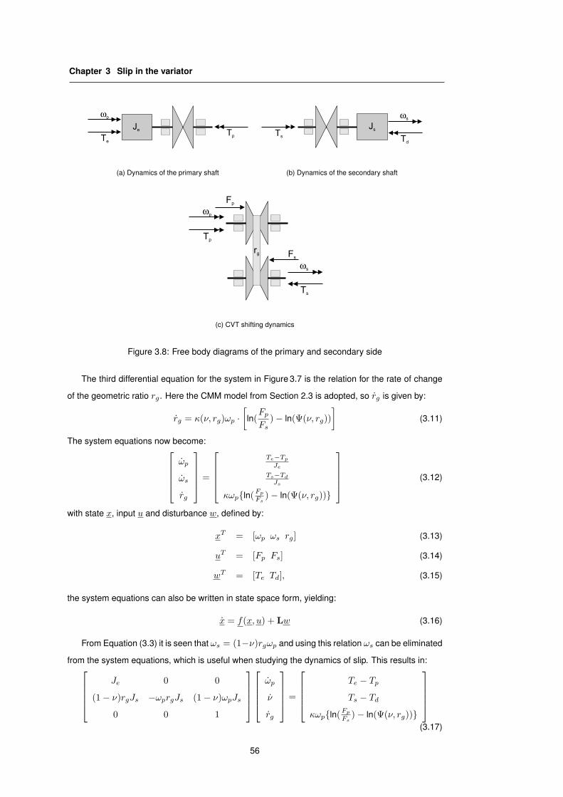
Chapter 3 Slip in the variator
Je
Te
ωp
Tp
(a) Dynamics of the primary shaft
JsTs
ωs
Td
(b) Dynamics of the secondary shaft
Tp
ωp
ωs
Ts
Fp
Fs
rg
(c) CVT shifting dynamics
Figure 3.8: Free body diagrams of the primary and secondary side
The third differential equation for the system in Figure 3.7 is the relation for the rate of change
of the geometric ratio rg. Here the CMM model from Section 2.3 is adopted, so rg is given by:
rg = κ(ν, rg)ωp ·[
ln(Fp
Fs) − ln(Ψ(ν, rg))
](3.11)
The system equations now become:⎡⎢⎢⎢⎣
ωp
ωs
rg
⎤⎥⎥⎥⎦ =
⎡⎢⎢⎢⎣
Te−Tp
Je
Ts−Td
Js
κωp{ln(Fp
Fs) − ln(Ψ(ν, rg))}
⎤⎥⎥⎥⎦ (3.12)
with state x, input u and disturbance w, defined by:
xT = [ωp ωs rg] (3.13)
uT = [Fp Fs] (3.14)
wT = [Te Td], (3.15)
the system equations can also be written in state space form, yielding:
x = f(x, u) + Lw (3.16)
From Equation (3.3) it is seen that ωs = (1−ν)rgωp and using this relation ωs can be eliminated
from the system equations, which is useful when studying the dynamics of slip. This results in:⎡⎢⎢⎢⎣
Je 0 0
(1 − ν)rgJs −ωprgJs (1 − ν)ωpJs
0 0 1
⎤⎥⎥⎥⎦
⎡⎢⎢⎢⎣
ωp
ν
rg
⎤⎥⎥⎥⎦ =
⎡⎢⎢⎢⎣
Te − Tp
Ts − Td
κωp{ln(Fp
Fs) − ln(Ψ(ν, rg))}
⎤⎥⎥⎥⎦
(3.17)
56
3.2 Dynamic Variator Slip Model
with state x, input u and disturbance w, defined by:
xT = [ωp ν rg] (3.18)
uT = [Fp Fs] (3.19)
wT = [Te Td], (3.20)
the system equations can also be written in state space form, yielding:
x = f(x, u) + L(x)w (3.21)
For subsequent analyses a linearization of the model around stationary working points is needed.
In each stationary working point x = 0, so ωp = 0, ν = 0 and rg = 0. From Equations (3.10), (2.5)
and (3.11) it then follows that1:
Te,0 = Tp,0 = 2μ(ν0, rg,0) min(Fp,0, Fs,0)Rp,0/ cos(β) (3.22)
Td,0 = Ts,0 = rg,0Tp,0 = rg,0Te,0 (3.23)
Fp,0 = Ψ(ν0, rg,0)Fs,0 (3.24)
For a unique specification of the stationary point it is necessary to prescribe the primary rotational
speed ωp,0, the geometric ratio rg,0, the driving torque Te,0 and the clamping force Fp,0 or Fs,0. The
slip ν0 then can be determined from Equation (3.22). In state space terms the stationary working
point is characterized by the state x0 = [ωp,0 ν0 rg,0]T , the input u0 = [Ψ(ν0, rg,0)Fs,0 Fs,0]T
and the disturbances w0 = [Te,0 rg,0Te,0]T .
Linearization requires that the partial derivatives of Rp = Rp(rg), μ = μ(ν, rg), Ψ = Ψ(ν, rg) and
κ = κ(ν, rg) are known. The derivative of Rp with respect to rg can readily be determined from
the geometric relations in Chapter 2. With respect to the experimentally determined functions μ, Ψ
and κ it is assumed that they are continuous and at least once differentiable with continuous partial
derivatives. Linearization of the system equations around a specified stationary working point then
results in:
δx = A0δx + B0δu + L0δw (3.25)
where δx = x − δx0, δu = u − δu0 and δw = w − δw0. Explicit relations for the entries of the
state matrix A0, the input matrix B0 and the disturbance matrix L0 are given in Appendix B.
1Quantities that refer to a stationary point are labelled with a subindex 0
57

Chapter 3 Slip in the variator
3.3. Ratio and Slip Estimation
This section describes some methods to estimate the geometric ratio rg and relative slip ν. The
geometric ratio and slip have to be estimated, because due to, for instance, pulley deformation,
temperature influences and belt deformation, they cannot be measured directly. The investigated
methods are:
• Pulley position measurement,
• Running radius measurement,
• Torque measurement,
• Normal load modulation,
• Engine load modulation.
Methods relying on the measurement of a geometric variable like pulley position or radial belt
position, of belt speed measurement or of torque measurement are used to estimate the geometric
ratio. Several authors have used pulley position measurement, (e.g. Kobayashi [47]) and running
radius measurement (e.g. Nishizawa [54]).
Differential speed measurement as used in some ABS systems try to distinguish between ratio
changes and slip by the speed at which the change occurs. Modulation methods are used to
estimate the slope of the traction curve. A normal load modulation method was proposed by Faust
[30].
After the overview of possible slip estimation methods a selection will be made based on this
overview and some measurements.
3.3.1. Estimation vs Measurement
Slip as defined in Definition 10 cannot be used, because the geometric transmission ratio cannot
be measured directly. The running radius of the belt on the pulley is in reality not constant along
the wrapped angle of the belt around the pulley and therefore not uniquely defined. Therefore the
ratio rg = Rp/Rs does not exist, since Rp and Rs are not uniquely defined.
In order to be able to estimate slip we need to define a measure for the geometric ratio and the
relative slip between belt and pulley.
Definition 11 The zero load ratio is defined by:
rs0 = rs, when Ts = 0 (3.26)
The zero load ratio rs0 can be seen as an estimate for the geometric ratio rg:
rg = rs0 (3.27)
58

3.3 Ratio and Slip Estimation
Proposition 1 The estimation of slip can be calculated with:
ν = 1 − ωs
ωprg(3.28)
Where ν is the estimation of relative slip between belt and pulley and rg the estimated geometric
ratio [47].
For the control of slip in a variator it is not necessary that the estimated value of slip is actually very
close to the ’real’ value of slip. What is needed is a relation between the estimated slip and the
variator efficiency that is known a priori.
3.3.2. Position measurement
If it is assumed that the change in pulley deformation due to changes in torque is negligible, a pulley
position or running radius measurement can be used to determine an estimate rg for rg.
To accurately estimate rg with a pulley position or running radius measurement, the position mea-
surement has to be compensated for temperature changes and for changing clamping force levels.
When the temperature rises, the transmission housing and all its parts will expand and the mea-
sured pulley position will change causing the estimated ratio rg to change due to the fact that the
sensor is mounted on the housing.
Clamping forces will have a large influence on the deformation of the pulleys, the belt and the hous-
ing. Therefore also this variable has to be taken into account when estimating rg from the pulley
position measurement.
The geometric ratio can be estimated using:
rg = f(xp,s, T, Fs) (3.29)
where f is a lookup table obtained by measurements of the zero-load ratio rs0 for different settings
of the pulley position xp or xs or the running radius Rp or Rs, the temperature T and the clamping
force Fs.
In Figure 3.9 a possible sensor position is shown for a running radius sensor. This sensor measures
the running radius at one location on the wrapped angle of the belt. Figure 3.10 shows a possible
configuration for the pulley position sensor [95].
3.3.3. Input/Output torque
The geometric ratio of the variator can also be approximated by the ratio of the input and output
torque of the variator. If the belt is cut in between the two pulleys, the forces on both sides must be
equal. The torque on the shafts is now given by the resultant of both belt ends:
Tp = (F2 − F1)Rp (3.30)
Ts = (F2 − F1)Rs (3.31)
59

Chapter 3 Slip in the variator
d
R
x
Movable
pulle
ysheave
Fix
ed
pu
lley
sh
ea
ve
Linear displacement sensor
Figure 3.9: Running radius sensor
d
R
x
Mo
va
ble
pu
lley
sh
ea
ve
Fix
ed
pulle
ysheave
Linear displacement sensor
Figure 3.10: Sensor setup for pulley position measurement
60

3.3 Ratio and Slip Estimation
x
d
R
Mo
va
ble
pu
lley
sh
ea
ve
Fix
ed
pu
lley
sh
ea
ve
T
To
rqu
ese
nso
r
Figure 3.11: Torque sensing method
Therefore, the ratio Tp over Ts is the same as Rp over Rs, the geometric ratio. The geometric ratio
rg can therefore be estimated by:
rg =Tp
Ts(3.32)
However, the torques are never measured directly after the variator, but rather on the shaft. There-
fore, the measured torque will include losses due to slip, bearings etc. Since no real variator is
completely lossless, the torque loss in the variator should be known to correctly use the torque
ratio as an estimate for the geometric ratio:
rg =Tp + Tloss
Ts(3.33)
here Tloss is the torque loss in the variator. This loss is caused by the losses in the belt and
the losses in the bearings. This method can only yield good accuracy for higher torques and is
therefore not suited for slip estimation in the lower torque regions.
Another disadvantage of this method is that torque measurement is expensive and error-prone and
therefore not very interesting in automotive transmissions.
3.3.4. Beltspeed
By measuring the beltspeed in addition to the pulley speeds, an estimate can be determined of slip
between belt and pulley [90]. If there is no slip and no other deformations occur, then rs = rg =ωs
ωp= Rp
Rs.
It is assumed that if slip occurs, the belt slips only on one pulley. The models presented in Chapter 2
suggest that slip will always occur on the pulley with the smallest running radius. However, these
models are simplifications of reality. Therefore it is not known a priori on which pulley this slip will
61

Chapter 3 Slip in the variator
occur, especially around rg = 1 this is unsure. Two situations must therefore be considered:
vsbelt = ωsRs (3.34)
vpbelt = ωpRp (3.35)
The running radius can be estimated by stating that if the slip occurs on one side, the running radius
on the other side is equal to the beltspeed divided by the rotational speed of that pulley:
Rs = vbelt/ωs (3.36)
Rp = vbelt/ωp (3.37)
With the geometric relation for the belt, given in Equation (2.1) the running radius on the other
pulley can be calculated.
νp = 1 − vbelt
vsbelt
(3.38)
νs = 1 − vpbelt
vbelt(3.39)
If it is assumed that slip between belt and pulley takes place at the secondary side, then we can
calculate the slip. This is a safe assumption, because if slip exists at the primary side, the estimated
slip value will be much higher than the real value. The comparison is shown in Figure 3.12. Of
course if slip exists only on the primary side this over estimates the slip by as much as 400%.
Therefore it should be known on which side the slip occurs.
There are several methods for measuring the speed of the belt. One way is to measure the
rotational speed of a wheel that runs on the belt. Another way is to measure the time between the
passing of two blocks. There are a few options to do this. One is to measure the passing by of the
airgap between the blocks using an inductive sensor on the outside of the belt when it runs on one
of the pulleys. The difficulty here is that the running radius is not constant, therefore the sensor
must follow the belt. Another option is to measure the passing by of the airgap between the blocks
on the inside in the straight part of the belt in between of the pulleys. If a chain is used, also the
passing of the pins on the side of the chain can be measured. In both of these cases the sensor
must follow the belt closely.
If a belt is specially constructed, with a few magnetic blocks, or with alternating differently shaped
blocks, then a hall-effect sensor can be used to measure the speed of the belt without the need to
follow the belt closely.
A sensor that measures the block pass frequency as described above must follow the belt closely.
Therefore, a mechanism must be used that is stiff in the running direction of the belt, but flexible in
all other directions. In Figure 3.16(a) such a device is shown for the inductive sensor.
3.3.5. Modulation methods
The frequency response functions of the variator will vary with the slope of the traction curve [66]
[56]. In a single operating point of the variator the slope of the traction curve can be viewed upon
62

3.3 Ratio and Slip Estimation
−0.1 −0.05 0 0.05 0.1−0.5
−0.4
−0.3
−0.2
−0.1
0
0.1
0.2
0.3
Slip [−]
Est
imat
ed s
lip [−
]
(a) Estimated slip with slip on secondary shaft (dashed:
assumed secondary side slipping, solid: assumed pri-
mary side slipping)
−0.1 −0.05 0 0.05 0.1−0.1
−0.05
0
0.05
0.1
0.15
Slip [−]
Est
imat
ed s
lip [−
]
(b) Estimated slip with slip on primary shaft (dashed:
assumed secondary side slipping, solid: assumed pri-
mary side slipping)
Figure 3.12: Estimated slip
63

Chapter 3 Slip in the variator
as being a viscous damping constant. This value influences the response of the output speed to
changes in the input speed. This form of slip estimation was introduced for CVT applications by
Faust et al. [30].
This method can be used to design an estimator for the slope of the traction curve. This slope is
different for micro- and macro-slip, therefore it is possible with this method to determine whether
the variator is in the micro- or in the macro-slip area.
For the modeling we look back at the slip model from Chapter 3. Assuming that the ratio remains
unchanged the variable states are given by: x = [ωp, ωs]T .
Normal load modulation
By linearizing in a certain working point a linear state space description is obtained. First, the
effective friction coefficient is taken piecewise linear. The sections of the curve where the traction
is increasing with increasing slip is the so called micro-slip area. The part of the traction curve
where the traction is constant or slightly decreasing with slip, is called the macro-slip area. Like in
Section 3.3, the traction coefficient can be approximated by:
μlin(ν, rg) = Mνν + Mrrg + M0 (3.40)
The state-space input is: u = [Fs]. The dynamic slip model, Equation (3.12), is linearized in point
x0 = [ωp0, ωs0]T .
x =
⎡⎣ − 2Mνωs0FsRp
ω2p0rg cos(β)Je
2MνFsRp
ωp0rg cos(β)Je
2Mνωs0FsRs
w2prg cos(β)Js
− 2MνFsRs
ωp0rg cos(β)Js
⎤⎦x + ...
... +
⎡⎣ − (2Mνν+2M0)Rp
cos(β)Je
(2Mνν+2M0)Rs
cos(β)Js
⎤⎦u (3.41)
y = Ix + 0u (3.42)
As can be seen from the bode plot of this system shown in Figure 3.13, the frequency responses of
the system with macro-slip are significantly different from the bode plot of the system in micro-slip.
Engine load modulation
Basically engine load modulation is the same method as the Normal Load Modulation, except that
the normal load is not modulated, but the driving torque. Because in Automotive applications this
happens naturally with IC engines when the explosion in the cilinder occurs, no additional actuation
is needed. Also the high frequency of the torque peaks from the engine give higher resolution than
the normal load modulation technique. This type of observer is also under investigation by Toyota
[98].
The input is now chosen as: u = [Te]. The dynamic slip model, Equation (3.12), is linearized in
64

3.3 Ratio and Slip Estimation
10−2
100
102
104
−400
−300
−200
−100
0
Mag
nitu
de [d
B]
10−2
100
102
104
−200
−100
0
100
200
Frequency [rad/s]
Pha
se [d
eg]
Figure 3.13: Transfer function ωp/Fs for different slip conditions (dashed macro-slip, solid micro-
slip)
point x0 = [ωp0, ωs0]T . The resulting system is:
x =
⎡⎣ − 2Mνωs0FsRp
ω2p0rg cos(β)Je
2MνFsRp
ωp0rg cos(β)Je
2Mνωs0FsRs
w2prg cos(β)Js
− 2MνFsRs
ωp0rg cos(β)Js
⎤⎦x + ...
... +
⎡⎣ 1
Je
0
⎤⎦u (3.43)
y = Ix + 0u (3.44)
The bode plots for the transfer function y1/u (ωp/Te) is shown in Figure 3.14. As for the normal
load modulation, also the modulation of the input torque can be used to determine the traction
conditions of the variator.
There is a distinct relation between the slope of the tractioncurve and this transfer function.
10−2
100
102
104
−200
−100
0
100
200
Mag
nitu
de [d
B]
10−2
100
102
104
−200
−100
0
100
200
Frequency [rad/s]
Pha
se [d
eg]
Figure 3.14: Transfer function ωp/Te for different slip conditions (dashed: macro-slip, solid: micro-
slip) [66] [56]
65

Chapter 3 Slip in the variator
3.3.6. Results
The pulley position measurement is used in this research for the estimation of the geometric ratio
and slip. In Figure 3.15 experimental results are shown using a LVDT sensor to measure the
pulley position on the primary side. In this figure is also shown a polynomial fit of the measured
sensor output vs. the measured zero-load ratio. Also shown is the drift of the sensor output with
respect to the temperature. This temperature dependence is quite large and should therefore be
compensated for. As can be seen from the graph, a linear fit gives a good estimation of this drift.
For the pressure, not shown in the graphs, also holds that its influence is not negligible and should
be compensated for. If these compensations are made good accuracy can be achieved for the slip
estimation.
In Figure 3.16 the measurement setup and measurements of the beltspeed are shown using an
inductive sensor placed close to the belt in between the pulleys. This type of measurement is
less sensitive to temperature and pressure, because if the beltspeed changes, so does the input
or output shaft speed. However, the pulley on which slip occurs is uncertain. This has to be
investigated further to make the beltspeed measurement method a reliable estimator for the slip
between belt and pulley.
The other techniques like the modulation technique are less accurate, due to the sensitivity for
noise in the case of the modulation technique and due to the unknown side on which slip occurs
for the beltspeed measurement. Also very high resolution measurements are required to make a
reliable estimation.
The torque measurement is only accurate for high torques and therefore not very interesting for
estimating the geometric ratio for slip control applications. Slip control is especially interesting for
low input torques, as will be explained in Chapter 4.
66

3.3 Ratio and Slip Estimation
0 2 4 6 8 10
0.6
0.8
1
1.2
1.4
1.6
1.8
2
2.2
LVDT Amplifier Voltage (V)
No−
load
rat
io r
s0 (
−)
(a) Measurements vs Polynomial fit (dashed line) of
the pulley position measurement output (LVDT) vs
the measured speed ratio at zero load (Ts = 0).
30 40 50 60 70 80 909.92
9.93
9.94
9.95
9.96
9.97
9.98
9.99
10
Oil Temperature (degrees Celcius)
LVD
T A
mpl
ifier
out
put (
V)
(b) Measurements vs Linear fit (dashed line) of the
temperature drift at a constant speed ratio at zero
load (Ts = 0).
Figure 3.15: Pulley position measurement and calibration
(a) Image of the beltspeed sensor.
200 400 600 800 1000 12000
1
2
3
4
5
6
7
8
9
t [s]
v [m
/s]
vb measured r
g
vb calculated
(b) Measurement of the beltspeed using an induc-
tive sensor. Shown are the transmission ratio, the
calculated beltspeed (no slip) and the measured
belt speed. The output torque is zero (Ts = 0).
Figure 3.16: Beltspeed measurement
67

Chapter 3 Slip in the variator
68

Chapter 4
Variator system losses
The efficiency of a variator is dependent on many factors. In this chapter all losses of the com-
ponents in a hydraulically actuated variator, including the actuation system, are assessed on their
contribution to the total energy loss. A mathematical model for the efficiency of a pushbelt type
variator is derived and the parameters are estimated. This model can be used to determine the
optimal operating points of a variator.
Earlier work on the efficiency of pushbelt variators include that of Micklem [53], who investigated
power losses in the variator as a function of pressure and speed, Akehurst [1] [2] [3], who showed
some detailed models of the loss mechanisms in the variator and Sue [81] who used Finite Element
Analysis to determine the influence of radial slip in the efficiency of the variator. In this chapter the
efficiency as a function of slip is investigated. As will be shown by measurements, the efficiency
can be seen as a function of a torque loss and slip. This model was earlier presented by Veen-
huizen [94], but here more detailed measurements are presented. Furthermore, the effects of a
hydraulic actuation system will be discussed. The actuation system has a large influence on the
overall efficiency and cannot be neglected.
The effect of efficiency optimization of the variator is discussed at the end of this chapter. The
optimum operating point can be used as a setpoint in a variator control system.
4.1. Losses
Losses in a variator and its actuation system can be attributed to different components. A hydraulic
actuation system needs a pump to generate hydraulic power. Other types of actuation systems
also require auxiliary power to operate. This power is not used to drive the car and is therefore
considered as a loss. Other losses occur in the bearings in the variator. These bearings are under
considerable load because of the clamping forces. These losses are considered ’torque losses’.
The variator itself also contributes to the power loss. Since it is a friction based drive there is always
some speed loss in the frictional contact. Also, internal friction in the belt or chain accounts for a
69

Chapter 4 Variator system losses
decrease in efficiency. These losses can be considered as a torque loss in the variator.
4.1.1. Efficiency of the variator
For power flow from primary to secondary pulley, the efficiency η of a variator is defined by:
η =Pout
Pin=
Tsωs
Tpωp(4.1)
If Tloss is denoted as all torque losses discussed earlier, and ωloss as the speed loss in the variator,
then using the torque loss and the speed loss the output torque and output speed can be calculated
by:
Ts =Tp
rg− Tloss (4.2)
ωs = ωprg − ωloss (4.3)
The efficiency of the transmission now becomes:
η =(
1 − rgTloss
Tp
)(1 − ν) (4.4)
4.1.2. Losses in the hydraulic actuation system
The power Ph consumed by a hydraulic pump without leakage as given in Equation (4.5) is there-
fore linear with both pressure pl and speed ωh of the pump shaft. The pressure is approximately
linearly dependent on the clamping forces. Furthermore, the hydraulic pumps used always have a
certain amount of leakage.
The pumping losses, Ph, are:
Ph = ωhcflpl + Tfr (4.5)
where cfl is the flow per rotation of the pump and Tfr is the friction torque of the hydraulic pump.
Lowering the pressure decreases the hydraulic loss in the transmission. In most production CVTs
the pump runs at a speed proportional to the engine speed. Because the CVT has to function
properly at idle speed, the pumped volume is higher than necessary in most driving situations.
4.1.3. Losses in the variator
To calculate the bearing losses SKF [73] supplies models and specifications. The frictional moment
of the bearings depends on the type of the bearing, the load, the speed of the axle and the type
and quantity of the lubricant used.
The bearings have a power loss that depends on the input speed and the load. Because the load
increases with input torque and therefore with input power and the speed also is proportional to the
input power, these have a constant influence on the efficiency with varying loads or speeds, but
there is also a constant friction part that accounts for very low transmission efficiencies at low input
70
4.3 Torque loss
power.
In a pushbelt speed and torque losses occur. These are caused by the bands running at a different
radius than the blocks. This difference in running radius causes a slip between the blocks and the
bands in ratios other than medium (rg �= 1). Also friction between the blocks account for some
losses. This has been discussed earlier in Section 2.2.2. Also chains and other types of belts have
internal friction when bending and stretching. These losses are also modeled in the parameter
torque loss.
The torque loss Tloss is not negligible, even not if the transmitted power is very small. Hence, the
variator efficiency is very low if the input torque Tp is small.
Speed loss is mostly caused by slip in the variator. The speed loss consists of the slip between the
belt and the pulley and the slip between blocks and bands. This slip is discussed in Chapter 3
4.2. Measurements
Efficiency measurements are shown in Figure 4.1. The testrig on which these measurements have
been performed is described in detail in Chapter 6. From the figure can be seen that the optimal
efficiency for different transmission ratios is found at different values of the slip.
The sensitivity of the efficiency for clamping force and speed are shown in Figures 4.2 and 4.3
respectively. Increasing speed has an adverse effect on efficiency as can be expected as does
increasing clamping force. If the clamping force is increased both the forces in the bearings and
the losses in the belt increase. However, as can be seen from Figure 4.3, the maximum efficiency
for the higher pressure setting increases. This effect is caused by the higher torque that can be
transmitted. The higher torque more than offsets the higher losses. When torque is constant
however, the efficiency will still decrease with higher clamping force.
Efficiency is optimal for slip speeds of around 1%, but the optimal value varies with clamping force
and ratio. Efficiency in medium (rg = 1), is much higher due to the absence of slip in the belt. Also
lower clamping forces give higher efficiency as can be expected, as does lower speed.
4.3. Torque loss
To obtain the torque loss from the measurements Equation (4.4) can be rewritten to:
Tloss =[1 − η
1 − ν
]Tp (4.6)
Tloss is calculated for the efficiency measurements shown in Figure 4.1, the results are shown in
Figure 4.4. With the torque loss estimation from the figure the efficiency can be estimated when the
primary torque is known. This torque however is itself a function of slip, clamping force and ratio.
To compare the efficiency measurements to the torque loss model first a model for the traction has
71

Chapter 4 Variator system losses
0 1 2 3 4 5 60.6
0.65
0.7
0.75
0.8
0.85
0.9
0.95
1
ν [%]
η [−
]
LOW OD
MED
Figure 4.1: Efficiency as a function of slip measured at rg = 0.43: solid line, rg = 1: dash-dotted
line and rg = 2.25: dashed line, with Fs = 8 kN and ωp = 225 rad/s
0 1 2 3 4 5 60.6
0.65
0.7
0.75
0.8
0.85
0.9
0.95
1
ν [%]
η [−
]
300 [rad/s]225 [rad/s]
150 [rad/s]
Figure 4.2: Efficiency as a function of slip measured at rg = 2.25 and Fs = 8 kN for ωp =
150 rad/s: solid line, ωp = 225 rad/s: dash-dotted line and ωp = 300 rad/s: dashed line
0 1 2 3 4 5 60.6
0.65
0.7
0.75
0.8
0.85
0.9
0.95
1
ν [%]
η [−
]
5 [bar]
8 [bar]
Figure 4.3: Efficiency as a function of slip measured at rg = 2.25 and ωp = 225 rad/s for Fs =
8 kN : solid line and Fs = 5 kN : dashed line
72

4.3 Torque loss
0 1 2 3 4 5 60
1
2
3
4
5
6
7
8
ν [%]
Tlo
ss [N
m]
Figure 4.4: Torque losses in the variator as a function of slip, solid: low ratio, dash-dot: medium
ratio and dashed: overdrive ratio (Fs = 8 kN , ωp = 225 rad/s).
0 1 2 3 4 5 60
0.02
0.04
0.06
0.08
0.1
0.12
ν [%]
μ [−
]
Figure 4.5: Traction curves as a function of slip for different ratios, solid: low ratio, dash-dot: medium
ratio and dashed: overdrive ratio (Fs = 8 kN , ωp = 225 rad/s).
0 1 2 3 4 5 60.7
0.75
0.8
0.85
0.9
0.95
1
ν [%]
η [−
]
Figure 4.6: Measurements of the efficiency as a function of slip for different ratios and the model fit,
solid: low ratio, dash-dot: medium ratio and dashed: overdrive ratio (Fs = 8 kN , ωp = 225 rad/s).
73

Chapter 4 Variator system losses
0 50 100 150 2000
0.5
1
1.5
2
2.5
3
3.5
Torque [Nm]
Pow
er lo
ss [k
W]
Final reduction loss
Variator torque loss
Pump driving power
Variator slip loss
Figure 4.7: Breakdown of the losses in a CK2 transmission.
to be known. The traction coefficient is modeled piecewise linear with slip. This approximation is
then used to calculate the torque through the variator depending on slip and ratio. The traction-
curve measurements and the linearized model are shown in Figure 4.5. In this graph three different
slopes are used to approximate the traction curve. More pieces give better accuracy.
4.4. Results
With this information the torque loss can be estimated by comparing the model to the efficiency
measurements. With the appropriate torque loss the efficiency model is evaluated using the given
functions in Equation (4.4). The result is plotted in Figure 4.6. With the dotted line the speed loss
due to slip is shown. Efficiency can not be higher than that line due to the slip loss.
From Figure 4.6 can be seen that the model gives a very good prediction of the variator efficiency
using a constant torque loss for a given transmission ratio, input speed and clamping force. Of
interest is further that the efficiency is much higher for medium ratio, than it is for low and overdrive
ratios. Maximum efficiency decreases with increasing clamping force or increasing input shaft
speed as can be expected.
4.5. Efficiency improvement potential
To estimate the efficiency improvement potential in a CVT that is currently in production, the model
is applied to a Jatco CK2 transmission [40]. In Figure 4.7 the different loss components are shown
for this transmission. From the figure it can be seen that the pump loss and the variator torque loss
are the major components in the CVT losses. By using energy optimized clamping force control
both the variator torque loss and the pump loss could be reduced. The variator torque loss is
optimized by the controller and the pump loss is reduced as a side effect due to the reduction in
clamping force and therefore in hydraulic pressure. In the lower torque region the variator torque
74
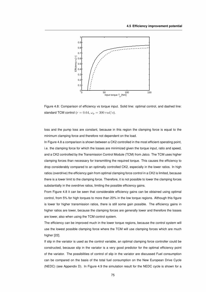
4.5 Efficiency improvement potential
0 50 100 1500
0.1
0.2
0.3
0.4
0.5
0.6
0.7
0.8
0.9
1
Input torque Tp [Nm]
Effi
cien
cyη
[−]
Figure 4.8: Comparison of efficiency vs torque input. Solid line: optimal control, and dashed line:
standard TCM control (r = 0.64, ωp = 300 rad/s).
loss and the pump loss are constant, because in this region the clamping force is equal to the
minimum clamping force and therefore not dependent on the load.
In Figure 4.8 a comparison is shown between a CK2 controlled in the most efficient operating point,
i.e. the clamping force for which the losses are minimized given the torque input, ratio and speed,
and a CK2 controlled by the Transmission Control Module (TCM) from Jatco. The TCM uses higher
clamping forces than necessary for transmitting the required torque. This causes the efficiency to
drop considerably compared to an optimally controlled CK2, especially in the lower ratios. In high
ratios (overdrive) the efficiency gain from optimal clamping force control in a CK2 is limited, because
there is a lower limit to the clamping force. Therefore, it is not possible to lower the clamping forces
substantially in the overdrive ratios, limiting the possible efficiency gains.
From Figure 4.8 it can be seen that considerable efficiency gains can be obtained using optimal
control, from 5% for high torques to more than 20% in the low torque regions. Although this figure
is lower for higher transmission ratios, there is still some gain possible. The efficiency gains in
higher ratios are lower, because the clamping forces are generally lower and therefore the losses
are lower, also when using the TCM control system.
The efficiency can be improved much in the lower torque regions, because the control system will
use the lowest possible clamping force where the TCM will use clamping forces which are much
higher [22].
If slip in the variator is used as the control variable, an optimal clamping force controller could be
constructed, because slip in the variator is a very good predictor for the optimal efficiency point
of the variator. The possibilities of control of slip in the variator are discussed Fuel consumption
can be compared on the basis of the total fuel consumption on the New European Drive Cycle
(NEDC) (see Appendix D). In Figure 4.9 the simulation result for the NEDC cycle is shown for a
75

Chapter 4 Variator system losses
0 200 400 600 800 1000 12000
1
2
3
Fue
l con
sum
ptio
n [g
/s]
0 200 400 600 800 1000 12000
200
400
600
Time [sec]
Tot
al fu
el c
onsu
mpt
ion
[g]
Figure 4.9: The results for the NEDC with slip control. The solid line is the result for an optimized
slip control with a low minimum pressure and the dashed line is the result for a CK2 with slip control.
CK2 transmission in a Nissan Primera. Using the engine characteristic, transmission losses and
control system used in Chapter 7, an estimation is made for the fuel economy of the Nissan Primera
with slip controlled CVT. The total is 516.5 g which means that on the NEDC the fuel consumption
was 6.6 l/100km. Compared to the data from Nissan (7.0 l/100km on the highway cycle and
8.8 l/100km in the combined cycle [55]). This is a large improvement. However, due to the limited
accuracy of the simulation probably the total gain will be less, but still significant.
4.6. Conclusions variator efficiency
To fully understand the efficiency potential of a CVT all losses in the variator were included in the
analysis. In Chapter 2 only the variator torque loss was examined. Also the losses of an actuation
system have to be taken into account when optimizing the efficiency of the CVT. If a hydraulic sys-
tem is used to actuate the CVT, also the losses caused by this system will be dependent on the
clamping force and therefore on the type of control that is used. A torque loss map is shown in
Figure 4.10.
From Figure 4.4 it was clear that the torque loss in the variator is independent from the value of
slip. The torque losses depend on the ratio rg, the input shaft speed ωp and the clamping force Fs.
Efficiency measurements of an hydraulically actuated CVT were already shown in Figure 4.6.
These measurements only show the variator efficiency, the pump losses have not been taken
into account. Finally, the efficiency including the pump losses is shown in Figure 4.11. Not only
are the maximum efficiencies lower, but also the level of slip at the maximum is higher. Using the
information in this figure the optimal operation points of this CVT can be found.
If these figures are compared to the traction curve measurements shown in Figure 4.5, it can be
76
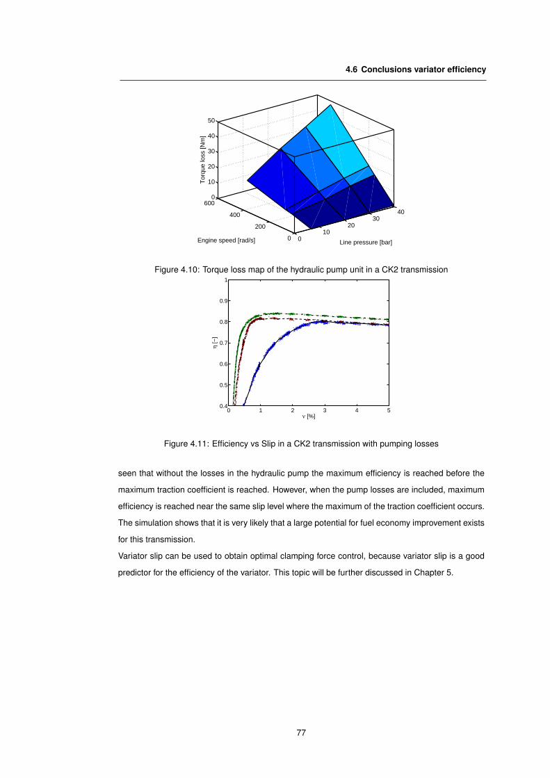
4.6 Conclusions variator efficiency
010
2030
40
0
200
400
6000
10
20
30
40
50
Line pressure [bar]Engine speed [rad/s]
Tor
que
loss
[Nm
]
Figure 4.10: Torque loss map of the hydraulic pump unit in a CK2 transmission
0 1 2 3 4 50.4
0.5
0.6
0.7
0.8
0.9
1
ν [%]
η [−
]
Figure 4.11: Efficiency vs Slip in a CK2 transmission with pumping losses
seen that without the losses in the hydraulic pump the maximum efficiency is reached before the
maximum traction coefficient is reached. However, when the pump losses are included, maximum
efficiency is reached near the same slip level where the maximum of the traction coefficient occurs.
The simulation shows that it is very likely that a large potential for fuel economy improvement exists
for this transmission.
Variator slip can be used to obtain optimal clamping force control, because variator slip is a good
predictor for the efficiency of the variator. This topic will be further discussed in Chapter 5.
77

Chapter 4 Variator system losses
78

Chapter 5
CVT Control
Control of slip is very common in automotive applications like traction control and anti lock braking
systems. However, slip control has not attracted much attention in the field of CVT systems until
now. Van Doorne’s Transmissie started investigating slip in a variator, in order to improve the
efficiency of the CVT. The problem of very high torques in geared-neutral transmissions around
the geared neutral point can be solved with slip control as well[93]. Until now the main problem
for implementation was that insufficient knowledge was available on measurement of slip in the
variator, which was discussed in Section 3.3, and the behavior of the variator under slip conditions,
which was discussed in Sections 3.1 and 3.2. Furthermore, until recently it was not known how
much slip the variator could withstand. Findings by van Drogen et al. [89] suggest that a metal
pushing V-belt can sustain a significant amount of slip for a substantial period of time.
The relation between slip and efficiency of the CVT was shown in Chapter 4. Here it was argued
that control of slip in the variator indeed offers appealing opportunities for efficiency optimization.
The relation between slip and traction shown in Chapter 3 is important for the understanding of the
slipping behavior of the variator.
In this chapter the control problem of a variator is discussed. First, a short overview of the current
control methods is given. Then, the most important properties of a clamping force control system
are discussed. Finally, some simulations are made to assess the possibilities of slip control in a
CVT.
In the next chapters several realizations of slip control will be discussed based on the slip dynamics
model and the transient variator model from Chapter 3. The first implementation of a slip controlled
variator is discussed in Chapter 6. Then in Chapter 7 an implementation will be shown in a CVT. In
Chapter 8, an implementation will be shown in a Nissan Primera.
79

Chapter 5 CVT Control
5.1. Control problem
As was shown in Chapter 4, the variator should be controlled at or very close to the maximum
traction point to achieve optimal efficiency in the case of a hydraulically actuated CVT as was
shown in Figure 4.11. However, controlling the variator at or near the maximum traction coefficient
is not trivial due to instability in that point.
The control problem of slip in a variator is similar to that of ABS systems, because the traction curve
of a variator is similar to the traction of a tire on the road. In the case of ABS several methods have
been used. Hybrid control methods like found in Automotive Control Systems [41] were the first
to be implemented. More recently, continuous control methods have been examined to improve
the performance and the comfort. For example the gain-scheduled LQR method [63] or the gain-
scheduled PI method [77] and optimal braking using the slip ratio [23]. Nonlinear control techniques
like sliding mode control [74] [49] [85] have also been examined for ABS systems. A special case
of sliding mode controllers, extremum seeking controllers, have been used for finding the maximum
traction point in ABS systems [26].
When operating the variator near the maximum traction point the stability of the open-loop system
is marginalized. The variator is stable when the traction curve has a positive slope as was shown
in Section 3.2. This is no longer the case at maximum traction. The non-controlled system will
become vulnerable to torque disturbances, because a small torque increase can put the variator in
the unstable area of the traction curve, which could result in very high slip values in the open loop
system.
There are uncertainties in the estimate of the maximum traction point. The traction coefficient will
not be constant over the lifetime of the variator. The changes due to the dependence of ratio,
pressure and speed can be compensated. The change over time however, is not exactly known.
5.2. Classic Clamping-force Control
Classic clamping force control in CVTs uses only feedback of the line-pressure, i.e. the secondary
cilinder pressure in most cases. The required clamping forces are determined offline, resulting
effectively in open-loop slip control. A lookup table is used to store the required clamping force
depending on the ratio and the engine torque. Because open-loop control is used, a margin is
needed in the clamping force to prevent disturbances to cause slip that could potentially cause
damage to the variator. This margin is called the safety-margin. This method is described well by
Vroemen [96].
In a CVT the belt is clamped by different forces on the primary and secondary axes. Ratio is held
by controlling the balance of these forces and slip is prevented by prescribing the absolute level
of the lowest of the two clamping forces. However, in most production CVT systems the clamping
force is controlled only with the secondary clamping force and the ratio is controlled by changing
80

5.2 Ratio control
the primary clamping force. The reason for this is that the clamping force ratio is greater than one
(Ψ > 1) for most operating points where slip might occur, as seen in Chapter 2. The clamping force
on the primary side is therefore mostly higher than on the secondary side.
A commonly used clamping force strategy is a so-called safety strategy. This method is designed to
keep the maximum torque capacity of the variator above the actual input torque at all times. Safety
with respect to V-belt type variators is defined as the torque margin between the current input
torque and the maximum transmittable input torque. This margin can be absolute, a safety torque,
or relative to the expected input torque, a safety factor. If an absolute margin is taken then the
minimally needed torque capacity of the variator needed to achieve this margin can be calculated
with:
Tmin = Tsf + |Tinput| (5.1)
Here Tsf is the safety torque. If the safety margin is taken relative to the input torque, then the
minimally needed torque capacity of the variator is:
Tmin = Sf |Tinput| (5.2)
where Sf is the safety factor. The safety needed depends on the uncertainty in the estimated input
and output torque and the expected input level of the disturbances.
Using Definition (9) the minimally needed clamping force can now be calculated with:
Fmin = TminRp cos β
2μmax(5.3)
If torque is very low, a minimum safety torque (Tsf ) of around 30 Nm to 50 Nm is used to prevent
slip in near zero-load conditions in the event of sudden shocks caused by for example road bumps.
Increasing the safety margin decreases variator efficiency as discussed in Chapter 4, therefore the
margin that should be kept depends on the desired robustness for torque load disturbances of the
variator. A typical safety vs. efficiency relation is shown in Figure 5.1.
Engine torque is estimated using the throttle input signal from the driver, the actual engine speed,
the state of the torque converter and an engine torque map. With this data a reasonable estimate
can be made for the engine torque. However, since it is an estimate a certain margin has to be kept
to be sure that modeling errors have no adverse effect. Also, sudden loads from the road can give
higher torques. Therefore a good margin is needed to be able to cope with these uncertainties. The
actual clamping forces applied to the pulleys (with r = 0) can be calculated from Ψ. The primary
and secondary clamping forces are given by:
Fp = max(Fmin, ΨFmin) (5.4)
Fs = max(Fmin,Fmin
Ψ) (5.5)
Over the lifespan of a variator the tribological properties will change. The maximum traction coeffi-
cient could decrease due to changes of the surface of the belt and the pulley and the traction fluid.
81

Chapter 5 CVT Control
1 1.5 2 2.50.6
0.65
0.7
0.75
0.8
0.85
Sf [−]
η [−
]
Figure 5.1: Safety factor vs. Efficiency given for three different transmission ratios.
An additional margin is needed to cope with these effects. Even if the driveline torque is measured,
a safety-factor substantially higher than 1 is still necessary.
5.3. Ratio control
The speed ratio of a variator is controlled by changing the balance of the clamping forces. For each
ratio there is a clamping force ratio for which the speed ratio of the transmission is constant as
explained in Chapter 2. If the clamping force ratio is changed with respect to this equilibrium point,
then the ratio of the transmission will change. A model for this was given in Section 2.3.
In modern CVTs the ratio is electronically regulated. The setpoint for the speed ratio of the transmis-
sion is determined by a predetermined algorithm. More on this issue can be found in Appendix E.
Mostly, a speed ratio map is used that is a compromise between fuel economy and driveability.
In this chapter and the following chapters the ratio control system will often remain unmentioned.
Although ratio control is used to keep the transmission in the correct position. No special attention
has been paid to this issue. The ratio control algorithm is assumed to be adequate.
The influence of ratio control on slip in the variator is not assumed to be negligible, but to keep
the initial control implementation simple, its effects are not taken into account. In Appendix A a
proposal for a control method is given that does take ratio changing into account.
5.4. Slip Control
One way of coping with the uncertainties of the driveline torque, the traction coefficient and reduc-
ing the safety-factor at the same time is slip control. With slip control the danger of unstable slip is
reduced using feedback control, while at the same time the clamping force is reduced, increasing
the efficiency.
The first step to slip control is estimation of slip in the variator. This topic was discussed in Chap-
ter 3. In this and the following chapters the pulley position measurement from Chapter 3 will be
82

5.4 Slip Control
used for estimation of slip. This method is chosen, because of the good accuracy and simplicity of
implementation.
The second step is the design of the controller. Two designs will be proposed. First, a slip control al-
gorithm is implemented on the beltbox testrig and second, a controller implemented in a production
CVT. In Appendix A, a nonlinear design is proposed that decouples and linearizes ratio changing
and slip. Stability, performance and robustness will be discussed.
Stability
First, the uncontrolled case is considered. To obtain a measure for the stability of the system the
eigenvalues are calculated. The system is stable in an operation point if the eigenvalues for that
point all lie in the left half of the complex plane.
For quasi-static situations (ωp = 0 and rg = 0), no losses and no disturbances, the eigenvalues
can be calculated from the linearized system matrix A0 from Section 3.2. Like in Section 3.3,
Equation (3.40), the effective friction coefficient is taken piecewise linear. Defining the state space
as x = [ν] and u = [Fs] and w = [Te, Td]T the system can be linearized around a certain
operating point x0 = ν0, resulting in a linear system given by:
δx = A0δx + B0δu + L0δw (5.6)
where δx = x − x0, δu = u − u0 and δw = w − w0. The eigenvalue of the system is given by
matrix A0. The linearized matrix A0 can now be derived (assuming ν0 � 1 and neglecting higher
order terms):
λ = A0 =1
ωp0
[−2Rs0F0Mν
Jt0 cos β
]with Jt0 =
(rg0
Je+
1Jsrg0
)−1
(5.7)
The eigenvalue is negative if Mν > 0, because Fs, Je and Js are always greater than zero.
Therefore, the system is stable for positive values of Mν and unstable for negative values of Mν .
For micro-slip (Definition 7) the system will be open-loop stable. If macro-slip occurs (Definition 8),
the slope of the traction curve will be zero or negative, resulting in an unstable open-loop system.
The control system should stabilize the slip in the variator in macro-slip.
Now the controlled case is considered. With a simple proportional controller with gain K, the
eigenvalue can be found to be:
λ =[
2(KpM0+F0Mν)((ν0−1)r2g0Js−Je)
Rp(rg0)rg0 cos(β)Jeωp0Js
](5.8)
To achieve stability the gain of the controller has to satisfy the following on the entire traction curve:
KM0 > −F0Mν (5.9)
Furthermore, stability is influenced by the bandwidth of the actuation system (i.e. the ’plant ca-
pacity’). In Figure 5.2 the frequency response function of the hydraulic actuation system in a CK2
transmission is shown. From this figure can be seen that the gain of the actuation system already
83

Chapter 5 CVT Control
Figure 5.2: Frequency Response Function of the hydraulic actuation system of the CK2 transmis-
sion and the fitted third order low pass filter
Figure 5.3: Damaged belt resulting from one of the experiments.
decreases starting at 5 Hz and the 180◦ phase lag is reached at 8 Hz. This will clearly limit the
achievable bandwidth. This could cause problems if the disturbances acting on the system, mainly
torque peaks, have a higher bandwidth than the actuation system. The effects of such disturbances
cannot be suppressed and could potentially cause high levels of slip.
Performance
High slip values can seriously damage the belt and the pulleys. An example of a damaged belt is
shown in Figure 5.3. Performance of the slip control system has to be good enough to keep the
peak levels of slip within allowable levels. The slip in the variator must not exceed these levels in
any situation, e.g. when the gas pedal is pressed suddenly, when moving from slippery surface to
rough, or when a pothole is hit.
The F-v failure diagram, as shown in Figure 5.4 [68] [89], gives the relation between the element
normal force and the absolute slip speed that indicates the boundary between adhesive wear and
mild wear. The product of these two variables gives a measure of the power absorbed in the
element-pulley contact for a certain friction coefficient (P = Fv). The limit of operation depends on
the temperature, lubrication, input speed and other factors and must be determined experimentally
as shown by van Drogen and van der Laan [89].
84

5.4 Slip Control
0 2 4 6 8 10 120
100
200
300
400
500
600
700
800
v [m/s]
FN [N
]
Figure 5.4: Example of a F-v failure diagram. The element normal force is given as a function of
the absolute slip (real speed difference between the belt and the pulley).
0 2 4 6 8 10−250
−200
−150
−100
−50
0
50
Figure 5.5: Torque peak from a road surface transition from an icy surface to a rough surface.
The variator can withstand some amount of slip given that the energy absorbed by the pulley-belt
contact can be dissipated in the belt and pulley. And the normal force - slip speed combination
should be below the adhesive wear boundary line. Here, ATF is used to cool the belt and pulley.
If slip in the variator is stabilized by a feedback controller, then the performance of this controller
must be sufficient to keep the slip below the critical line from the F-v diagram (Figure 5.4). The
difficulty is to do this for unknown disturbances caused by the road-wheel contact. These distur-
bances include torque peaks from crossing speed-bumps, suddenly changing tire friction due to
road surface changes (ie going from slippery to rough surface) and μ-split situations. Disturbance
rejection should be strong enough to keep the slip in the variator below the critical slip limit for all
disturbances from the drivetrain. In Figure 5.5 an example is given of a surface transition torque
peak.
85

Chapter 5 CVT Control
Robustness
The control system will be designed using the slip dynamics model derived in Chapter 2. Modeling
inherently introduces errors with respect to reality. These errors can be divided into two categories,
the first one is unmodeled dynamics, the second one is parametric errors.
Unmodeled dynamics are caused by simplifications of the physical properties of the system or
unknown properties of the system. If a linearized model is used, the nonlinear parts of the system
are left out and are thus cause for unmodeled dynamics. Parametric errors occur when parameters
of the model are not identified properly. This can be caused by limited accuracy of the estimation,
or by varying parameters.
The control design should be robust for these modeling uncertainties and parameter errors. By
demanding a maximum sensitivity of the closed loop system, robustness can be achieved for model
imperfections, unknown parameters and aging effects.
5.5. Simulation
The feasibility of slip control is tested using simulation. The simulation model, with a structure as
shown in Figure 5.6(b), is a combination of the variator model, the traction model and the slip-
dynamics model as discussed in Chapter 2 and Chapter 3. The Matlab R© /Simulink R© model is
shown in Figure 5.6(a). Also the Delft Tyre model is used for road-load simulation [43] [69].
In Figure 5.7 the results are shown for the classic clamping force control system. A vehicle driving
over a bump of 15 cm height is simulated. Plots for a safety-factor of 1.3, 1.5 and 2.0 are shown
in this figure. In Figure 5.8 the same simulation is performed with a slip control strategy. The
simulation is based on an input shaft torque of Tp = 200 Nm, a CVT model based on the CK2
transmission and a vehicle that hits a 10cm bump at v = 17m/s. The torque peak that is generated
is more than 150 Nm at the variator output shaft.
From these figures can be seen that with a normal safety strategy the slip is only limited using high
safety factor, i.e. around 2.0. If a slip control strategy is applied, actuation bandwidth is essential.
In Figure 5.8 several graphs are shown with varying bandwidth. From this figure can be seen that
higher actuation bandwidth gives better results, reducing the slip peak to around 10%, comparable
to a safety factor of 1.5. In the case of slip control an effective safety factor of 1.0 is used. This
means that the clamping force is lower, resulting in less danger of damage for the same amount of
slip for the variator.
In Figure 5.9 the result of torque peaks caused by sudden throttle actuation. In this graph the results
for the different control strategies are shown in response to a 150 Nm engine torque increase. A
comparison is shown for the situation of a slip controlled variator with and without feedforward.
A feedforward is added based on a safety-factor strategy with a safety-factor of 1. This almost
completely eliminating dangerous slip peaks, where in the case of only feedback slip control slip
86

5.5 Simulation
11
x_s
10
x_p
9
GO
8
T_sec
7
T_pri
6
Tq_sec
5
Tq_pri
4
p_s
3
p_p
2
dq_M2
1
dq_M1
p_in
w
p
F
sec_hydraulics1
p_in
w
p
F
sec_hydraulics
B_p(s)
A_p(s)Transfer Fcn4
B_p(s)
A_p(s)Transfer Fcn3
B_dq(s)
A_dq(s)Transfer Fcn2
B_dq(s)
A_dq(s)Transfer Fcn1
Tb
slip
r
Tp
Ts
eta
Torque
Scope1
Scope
r
x_p
x_s
Pulley sensor
T_acc
T_brake
w
M2
T_acc
T_brake
w
M1
wp
Tp
Fp
Fs
r
Rp
Ide
90
Constant
w1
w2
r
Fs
Rp
T
slip
Belttorque
Band-LimitedWhite Noise5
Band-LimitedWhite Noise4
Band-LimitedWhite Noise2
Band-LimitedWhite Noise1
6
Reset
5
GO2
4
T2_in
3
T1_in
2
servoventiel sec
1
servoventiel prim
Fp
wp
T2
T1
Fs
(a) Matlab R© /Simulink R© model of the variator
CVT VehicleEngine
Control
Throttle Road surface
Slip, Ratio
Clamping force
Te
ωp Td
ωd
(b) Simulation Structure
Figure 5.6: Simulation details
87
Chapter 5 CVT Control
increases to around 10% due to the sudden change in engine torque.
5.6. Conclusions and recommendations variator control
In the first simulations the driven tires come completely off the ground and start spinning, when they
touch the ground again the wheels are suddenly slowed at the friction limit of the tires, effectively
the wheels are slipping. This is one of the most severe incidences that cause large torque peaks
in the driveline. Also torque peaks that are caused by suddenly stepping on the throttle can cause
large torque peaks. Although the torque peaks are not quite as high as the wheel slip situation, the
duration can be much longer.
The simulations showed that a control system using a constant safety-factor is also vulnerable for
high slip peaks caused by severe torque peaks. Also from the simulations can be seen that the
bandwidth of the actuation system is a very important factor for slip control in a V-belt type variator.
If the bandwidth is too low, torque peaks from the road cannot be compensated. The simulation of
driver induced torque peaks shows that when a slow slip controller is used, this can cause serious
problems with large amounts of slip. However, a feedforward control action can reduce this risk in
this kind of predictable torque peaks.
88

5.6 Conclusions and recommendations variator control
2.3 2.35 2.4 2.45 2.5 2.55
0
5
10
15
Time [s]
ν [−
]
Figure 5.7: Simulation of vehicle driving over a 15 cm high obstacle using a safety-factor clamping
force strategy (solid: Sf = 1.3, dash-dot: Sf = 1.5, dashed: Sf = 2.0).
2.3 2.35 2.4 2.45 2.5 2.55
0
5
10
15
Time [s]
ν [−
]
Figure 5.8: Simulation of vehicle driving over a 15 cm high obstacle using slip control (solid: 7 Hz
bandwidth actuation, dashed: 20 Hz bandwidth actuation.
2.4 2.5 2.6 2.7 2.8 2.9 3 3.1 3.2
0
5
10
15
Time [s]
ν [−
]
Figure 5.9: Simulation of a driver induced torque peak, engine torque going from 50Nm to 200Nm
in 0.1 s for different control strategies (solid: safety-factor, dash-dot: slip control (7 Hz), dashed:
slip control with feedforward (7 Hz)).
89

Chapter 5 CVT Control
90

Chapter 6
First generation slip controlledvariator
Slip control is first implemented on the variator test rig [8], [11]. This test rig allows fast control of
the clamping force and accurate measurement of the pulley position. Also the possibility exists to
use fixed transmission ratio using so-called ratio rings. Because the ratio is fixed, the ratio changing
of the variator can be neglected for the controller design. This setup is also used for the measure-
ments of the traction curves and the efficiency shown in previous chapters.
This chapter will focus on the first implementation of slip control in a variator. First, the setup is
described, then the control implementation is explained. Finally, the experimental results from the
measurements on the test rig will be shown and some conclusions will be drawn.
6.1. Experimental setup
The experiments in this chapter are done on the test rig shown in Figure 6.1 and schematically
represented in Figure 6.2. This test facility comprises two identical asynchronous electric mo-
tors with a maximum power: 78 kW , maximum torque of 298 Nm and a maximum speed of
525 rad/s 5000 rpm. The pressure in the primary and secondary hydraulic cylinders of the
variator can be controlled independently between 1 bar and 50 bar. The primary and secondary
pressure are independently controlled using two Bosch-Rexroth solenoid valves. The hydraulic
pressure directly controls the clamping force on the pulley.
The variator used in this setup is a Van Doorne’s Transmissie beltbox type Alaska P811. The pulley
shafts in this transmission have an axial distance of 155 mm and the length of the belt is 650 mm.
The primary cilinder area, Ap, is 259.8 cm2 and the secondary cilinder area, As, is 124.0 cm2.
The pulley angle is 11o. This beltbox is lubricated and cooled using Automatic Transmission Fluid
(ATF).
91
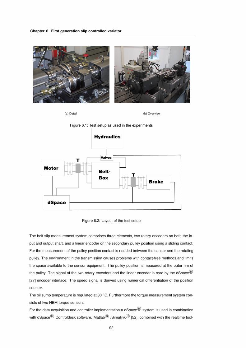
Chapter 6 First generation slip controlled variator
(a) Detail (b) Overview
Figure 6.1: Test setup as used in the experiments
Belt-
Box
Motor
Brake
Hydraulics
Valves
dSpace
T
T
Figure 6.2: Layout of the test setup
The belt slip measurement system comprises three elements, two rotary encoders on both the in-
put and output shaft, and a linear encoder on the secondary pulley position using a sliding contact.
For the measurement of the pulley position contact is needed between the sensor and the rotating
pulley. The environment in the transmission causes problems with contact-free methods and limits
the space available to the sensor equipment. The pulley position is measured at the outer rim of
the pulley. The signal of the two rotary encoders and the linear encoder is read by the dSpace R©[27] encoder interface. The speed signal is derived using numerical differentiation of the position
counter.
The oil sump temperature is regulated at 80 oC. Furthermore the torque measurement system con-
sists of two HBM torque sensors.
For the data acquisition and controller implementation a dSpace R© system is used in combination
with dSpace R© Controldesk software. Matlab R© /Simulink R© [52], combined with the realtime tool-
92

6.2 Control implementation
Table 6.1: Measurement equipment for angular speeds and sheave position.
Measurement Sensor Resolution
Sec. pulley position Heidenhain ST3078 1 μm
Incremental encoders Heidenhain ERN 1381 1/2048 rad
Torques HBM T20WN 200Nm 0.2 Nm
box, is used for the programming of the dSpace R© system.
The clamping forces fp and Fs are controlled by the hydraulic pressure. The pressure is measured
at the hydraulic input side of the cilinders. The pressure inside the cilinders however, is also depen-
dent on the shaft rotational speed. This is due to the centrifugal force acting on the oil inside of the
cilinder. To maintain the required clamping forces, the pressure caused by the rotational speed of
the shaft is deducted from the required pressure calculated by p = F/A (the pressure is therefore
calculated by: p = F/A − fcω2). The primary and secondary cilinder pressures are controlled
using two independent servo-loops.
6.2. Control implementation
6.2.1. Introduction
The variator has two control inputs: Fp and Fs, the primary and secondary clamping force respec-
tively, and two outputs: ν and xp, the slip and the transmission ratio respectively. In Figure 6.3 the
block diagram is shown of the control system.
The geometric ratio is controlled using the clamping force ratio as the control output and the posi-
tion of the primary pulley as the control input. For the controller is chosen for an integral controller
with low gain. During the tests the reference of the ratio is kept constant. This is done to prevent
instability the ratio control loop and minimize the ratio control loop influence on the slip control loop.
The slip is controlled using the secondary clamping force as the control output and the absolute
slip as the control input. For this implementation is chosen for a PI controller for the slip control
loop. A differentiating control action is omitted, because of the noise in the control input signal. In
this setup slip is estimated using the primary and secondary shaft speeds and the primary pulley
position measured by the linear encoder. The absolute value of the slip is taken, because the slip
should be maintained for both positive and negative torques, causing positive and negative slip
respectively.
6.2.2. System identification
Using measurements of the frequency response of the system, the characteristics of the system
are identified. These measurements are done by adding noise to the output signal of the controller.
With the measured input of the system and the measurement of the system output, the process
93

Chapter 6 First generation slip controlled variator
X
xp
Fs
Fp
+
+
ref
xref Exp
-
-
Figure 6.3: The block diagram of the control loop.
sensitivity function is obtained. The process sensitivity function is defined as:
S(s) =G(s)
1 + C(s)G(s)(6.1)
with C(s) equals Cs in Figure 6.3 and G(s) equals combination of the actuator dynamics and the
variator slip dynamics. Sensitivity of the controlled system was measured by adding band-limited
noise to the controller output signal. By estimating the transfer function of the noise to the plant
output signal an estimate for the process sensitivity is obtained. The plant characteristics can be
deducted from the process sensitivity function with G = S1−SC . The measured sensitivity of the
system for the clamping force control is given for 0.5% slip in Figure 6.4. The ratio of the CVT
was near overdrive (rs ≈ 2). The primary speed was 50 rad/s. The sensitivity for 0.5% slip is
low for very low frequencies and has a dip at 1.5 Hz. The process FRF is shown in Figure 6.5.
The process at 0.5% has an eigenfrequency of 1.5 Hz. This frequency strongly depends on the
inertia on the driveshaft (normally including the vehicle mass). From the first order model a first
order response was expected. The measurement results support this. The slope of the process
FRF goes to roughly -1 for high frequencies, with a phase shift of -90 degrees.
6.2.3. Controller tuning
Stability is achieved using a proportional feedback. Integral gain is added to increase the gain at
low frequencies. Other than the proportional gain no other filters are used. The gains are given by:
Control action Gain
Proportional 5000 N
Integral 8000 N/s
94

6.3 Experimental results
100
101
−30
−20
−10
0
10
Mag
nitu
de [d
B]
100
101
−200
−100
0
100
200
Frequency [Hz]
Ang
le [d
eg]
Figure 6.4: Sensitivity of slip controlled system at 0.5% slip
100
101
−200
−180
−160
−140
−120
−100
Mag
nitu
de [d
B]
100
101
−200
−100
0
100
200
Frequency [Hz]
Ang
le [d
eg]
Figure 6.5: Frequency response of slip controlled plant at 0.5% slip
6.3. Experimental results
On the Beltbox testrig a slip controlled variator is tested for robustness in torque peaks from the
driveline. In Figure 6.6 the results from this test are shown. It shows the response of the variator
slip to several peaks in the torque at the CVT output side. The primary drive shaft of the variator
is controlled at a constant speed. The primary and secondary pressures are controlled by the slip
control algorithm.
From this figure it can be seen that peaks in the torque also cause peaks in the slip signal. This
is unavoidable, because no prior knowledge of the disturbances is available and the controller can
only react to the measured slip value. The slip control algorithm reacts to the increase in slip by
raising the clamping pressure, thereby reducing slip. The amount of slip that is reached is therefore
highly dependent on the bandwidth of the closed loop system. From the figure can be seen that
slip increases only slightly and is reduced in a short period of time.
95

Chapter 6 First generation slip controlled variator
210 220 230 240 250 260 270 280 290 3000
5
10
ν [%
]
210 220 230 240 250 260 270 280 290 3000
50
100
150
Tp [N
m]
210 220 230 240 250 260 270 280 290 3000
20
40
Time [s]
FN [k
N]
Figure 6.6: The slip and clamping force response of the variator to torque steps and peaks. The
upper graph shows the slip as a function of time, the middle graph shows the input torque as a
function of time and the lower graph shows the clamping force as a function of time.
In this measurement torque peaks of up to 50 Nm are shown and steps of up to 30 Nm. The
resulting slip peaks are between 2% and 6%, which is in the safe area of the F-v diagram.
The efficiency of the variator is tested on the beltbox testrig. The results have already been shown
in Figure 4.6 in Chapter 4. The variator efficiency can be over 90% for higher torque levels. The
pressure in the beltbox testrig is not constrained to a minimum, so maximum efficiency can be
reached until very low torques. However, the bandwidth of the hydraulic system depends also on
the nominal pressure level. For pressures lower than 3 bar the bandwidth was too low for stable
control. Therefore lower torque levels will cause lower transmission efficiency.
6.4. Conclusions and recommendations first implementation
The first implementation of slip control is fairly rudimentary. However, it shows that slip control in a
pushbelt type variator is feasible. The experimental results show that the variator can be controlled
in a stable way in an operating point in the part of the traction curve that is decreasing. Further-
more it was shown that a slip controlled variator can be robust for disturbances in the form of torque
peaks and steps.
In this first implementation it was found that the response of the hydraulic system at low pressure
was slower than its response at high pressure. This was a limitation, because the system can no
longer react to torque peaks in time to prevent high values of slip. Therefore it is recommended
that a minimum pressure is maintained to avoid this problem.
The response of the slip in the variator to torque peaks and to changes in clamping force varies
96

6.4 Conclusions and recommendations first implementation
with the ratio and the rotational speed. Performance of the slip control system could be improved
by using gain scheduling to make use of these variations. Load disturbances did not cause very
large slip peaks and slip was regulated both in the macro-slip area and the micro-slip area. The
system was tested with torque peaks of up to 50 Nm and steps of up to 30 Nm primary torque.
97

Chapter 6 First generation slip controlled variator
98

Chapter 7
Gain scheduled PI control of slip ina CVT
After the successful implementation of slip control on the beltbox testrig, slip control on a full CVT
transmission is attempted [9], [64], [65]. The transmission that is used in the CVT transmission
testrig is a CK2 transmission from Jatco. This transmission is different with respect to the beltbox.
The transmission contains several components that the beltbox does not: a torque converter, a
DNR set, intermediate shaft and the differential gear. The main differences between the variators
of these two are the hydraulic system, the size of the pulleys and the speed and position measure-
ment system.
Implementation of slip control in a production model CVT is more difficult than its implementation on
the beltbox testrig, mainly because of the slower hydraulic system response. The slower response
severely limits the achievable bandwidth of slip control system. Also there is a minimum hydraulic
line pressure. The ratio control system of the factory supplied transmission control unit is used and
the ratio control itself will not be taken into account.
In this chapter first the details of the transmission testrig will be explained. Then the implementa-
tion of the control system will be reviewed. The approach from Panagopoulos [60] and Solyom [75],
which they used for ABS control design, is used for controller synthesis. This method ensures sta-
bility of the closed loop system for a system with a cone bounded uncertainty, while maximizing
disturbance rejection. The experimental results will be shown and finally, some conclusions and
recommendations will be given for this chapter.
7.1. Transmission testrig
The reference transmission is tested on a testbed with the complete driveline of a Nissan Primera.
The layout of this testbed is shown in Figure 7.1. This testbed is fitted with a 2.0 litre IC engine
99

Chapter 7 Gain scheduled PI control of slip in a CVT
from a Nissan Primera, the CK2 transmission, the driveshafts, a flywheel and both a hydraulic disc
brake and an eddy current brake.
With the flywheel, the vehicle mass is simulated and with the eddy current brake the road-load or
other loads can be simulated. The disc brake is used to simulate emergency braking.
Limitations of this testrig are the limited bandwidth of the braking system. Also because of the
flywheel fixed to the axis no wheelslip situations can be simulated.
The testrig is equipped with a torque sensor between the engine and the transmission. This sensor
uses strain gages for measurement of torsion. The signals are transferred using a wireless con-
nection. The same system is used for the torque measurement on the driveshaft.
Engine speed, primary speed, secondary speed and driveshaft speed are measured using the build
in sensors of the engine and the transmission respectively. These sensors use hall-effect sensors
to measure the rotational speeds.
Furthermore, the pulley position on the primary side is measured using a Linear Variable Differen-
tial Transformer (LVDT), a capacitive linear displacement sensor.
A dSpace R© system is used to control the CK2 transmission, the engine throttle and the brakes.
Also the original Transmission Control Module (TCM) can be used for comparison.
The 4 cilinder 2.0litre IC engine has a maximum torque of 181Nm at 5000 rpm and can deliver op
to 104 kW of power at 6000 rpm. The maximum torque curve is shown in Figure 7.2.
The efficiency-map of the engine is shown in Figure 7.2. With this efficiency-map an optimal oper-
ation line (OOL) can be calculated. The OOL is also shown in this figure. The OOL can be used
as a reference for the engine speed for a given output power level. With the optimal engine speed
and output speed an optimal transmission ratio can be calculated.
7.2. Control implementation
On the above described transmission testrig, slip control is implemented. First, a linearized dynamic
model for slip is used to analyse the system. Then, a controller is designed using a robust PI-
controller synthesis method.
7.2.1. Slip model
The torque generated on both shafts of the variator can be conveniently described on the basis
of Equation (3.10). Note that by using this description, torque losses are neglected. Although this
limits model accuracy, the effect of torque loss is assumed small enough and not significant for the
description of the variator dynamics. It is also assumed that speed ratio changes due to the axial
motion of the variator sheaves are much smaller than those associated with slip. This assump-
tion may impose limitations on the control strategy derived below, for those cases where fast ratio
changes occur. This assumption allows the contribution of rg to ν to be neglected. The slip dynam-
ics from Section 3.2 can now be simplified. The simplified model is derived using Equations (3.3)
100

7.2 Control implementation
(a) Schematic of the TR3 testbed (b) Picture of the TR3 testbed
Figure 7.1: Layout of the TR3 testbed
101

Chapter 7 Gain scheduled PI control of slip in a CVT
245
250
250
250
255
255
255
255
260
260
260
260
260
270
270
270
270
270
270
280
280
280
280
280
280280
300
300
300
300
300
350
350
350
350
400400
400
500500
500
Engine Speed [rpm]
Eng
ine
Tor
que
[Nm
]
1000 2000 3000 4000 5000 6000
20
40
60
80
100
120
140
160
180
200
220
Figure 7.2: Efficiency map of the 2.0litre IC engine mounted on the TR3 testbed, also the OOL
(dashed line) and the maximum torque curve (solid line) are shown.
and (2.6), resulting in:
ν = − rs
rg(7.1)
In this equation the rate of change of the speed ratio in terms of the system states is given by:
rs =ωsωp − ωsωp
ω2p
. (7.2)
The dynamics of the variator as shown in Figure 3.7 were derived Chapter 3. If the ratio changing
of the variator is considered to be much smaller than the dynamics of slip, then the model derived
in Chapter 3 can be simplified. Substituting Equations (3.10), (7.2), (3.8) and (3.9) in Equation (7.1)
leads to the following description of the slip dynamics:
ν =1ωp
(−2FsRsμ(ν)
cos(β)Jsrg+
Td
Jsrg
)+
(1 − ν)ωp
(−2FsRsrgμ(ν)
cos(β)Je+
Te
Je
)(7.3)
This equation is non-linear in ν. By linearizing this equation at a certain operating point a linear
state space representation is derived [44].
Linearized model
Like in Section 3.3, Equation (3.40), the effective friction coefficient is taken piecewise linear. Defin-
ing the state space as x = [ν] and u = [Fs] and w = [Te, Td]T the system can be linearized
around a certain operating point x0 = ν0, resulting in the linear system:
δx = A0δx + B0δu + L0δw (7.4)
where δx = x − x0, δu = u − u0 and δw = w − w0. The linearized matrices A, B and L can now
be derived (assuming ν0 � 1 and neglecting higher order terms):
A0 =1
ωp0
[−2Rs0F0Mν0
Jt0 cos β
]with Jt0 =
(rg0
Je+
1Jsrg0
)−1
(7.5)
B0 =1
ωp0
[−2Rs0μ(ν0)
Jt0 cos β
](7.6)
102

7.2 Control implementation
L0 =1
ωp0
⎡⎣ 1
Je
1Jsrg0
⎤⎦
T
(7.7)
The derived linearized system will be used for controller design. The system matrix A indicates that
stability requires Mν to be positive. This is only the case in the micro-slip region, which is the main
reason for its common use in production CVT’s. A control action is needed in order to stabilize the
system in the macro-slip region.
The model has 3 inputs, but only the clamping force Fs can be controlled on implementation. In a
vehicle application, the input torque Te is controlled by the driver via the throttle pedal and the output
torque Td is determined by road conditions. Therefore they must be regarded as disturbances
acting on the system. If an electronic throttle controller is used, then this would possibly eliminate
the disturbance from the engine torque. This is not investigated further in this thesis.
System analysis
From the linearized system can be seen that the dynamics of slip depend on:
• the slope of the traction curve Mν ,
• the input shaft speed ωp,
• the transmission ratio rg,
• the running radius Rs and
• the clamping force Fs.
From the system matrix A0 can be seen that the system has a stable pole when the slope of the
traction coefficient Mν is positive, which will move to the RHP for negative values of Mν . The other
values in the system matrix are always positive. This means that the controller should stabilize all
possible negative values of Mν .
The dynamics of slip are scaled by the input shaft speed as can be seen from Equation (7.3). A
controller gain proportional with the input shaft speed would simplify the control design problem,
because it eliminates ωp from the equation. A gain scheduling approach with respect to ωp can
therefore be useful.
The dynamics further depend on the transmission ratio rg and on Rs. Rs is in turn a function of
rg. Matrix B0 is negative for positive values of slip. This means that an increase in clamping force
leads to a decrease in slip, which is intuitive. This can be seen as a phase shift of 180◦ in the bode
plots.
The proposed variator control scheme is shown in Figure 7.3. The slip control system consists
of a controller C, the actuator dynamics G2 and the slip dynamics G1. In Figure 7.4 several
(open-loop) bode plots are shown for different operating points of the linearized Plant. The first
plots show the difference between the response of the system in micro- and macro-slip. In the left
103
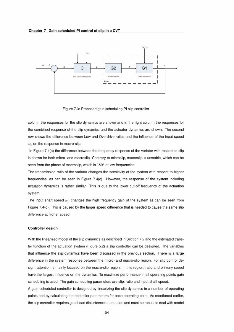
Chapter 7 Gain scheduled PI control of slip in a CVT
C G2 G1
Gain Scheduled PI-Controller Actuator dynamics Variator slip dynamics
p
ref
rs0
Te, Td
Plant
-
+e u F
Figure 7.3: Proposed gain scheduling PI slip controller
column the responses for the slip dynamics are shown and in the right column the responses for
the combined response of the slip dynamics and the actuator dynamics are shown. The second
row shows the difference between Low and Overdrive ratios and the influence of the input speed
ωp on the response in macro-slip.
In Figure 7.4(a) the difference between the frequency response of the variator with respect to slip
is shown for both micro- and macroslip. Contrary to microslip, macroslip is unstable, which can be
seen from the phase of macroslip, which is 180o at low frequencies.
The transmission ratio of the variator changes the sensitivity of the system with respect to higher
frequencies, as can be seen in Figure 7.4(c). However, the response of the system including
actuation dynamics is rather similar. This is due to the lower cut-off frequency of the actuation
system.
The input shaft speed ωp changes the high frequency gain of the system as can be seen from
Figure 7.4(d). This is caused by the larger speed difference that is needed to cause the same slip
difference at higher speed.
Controller design
With the linearized model of the slip dynamics as described in Section 7.2 and the estimated trans-
fer function of the actuation system (Figure 5.2) a slip controller can be designed. The variables
that influence the slip dynamics have been discussed in the previous section. There is a large
difference in the system response between the micro- and macro-slip region. For slip control de-
sign, attention is mainly focused on the macro-slip region. In this region, ratio and primary speed
have the largest influence on the dynamics. To maximize performance in all operating points gain
scheduling is used. The gain scheduling parameters are slip, ratio and input shaft speed.
A gain scheduled controller is designed by linearizing the slip dynamics in a number of operating
points and by calculating the controller parameters for each operating point. As mentioned earlier,
the slip controller requires good load disturbance attenuation and must be robust to deal with model
104

7.2 Control implementation
10−2
10−1
100
101
102
−220
−200
−180
−160
−140
Mag
nitu
de [d
B]
10−2
10−1
100
101
102
0
90
180
Frequency [Hz]
Pha
se [d
eg]
(a) microslip (solid) vs macro-slip (dashed) G1
10−2
10−1
100
101
102
−300
−200
−100
Mag
nitu
de [d
B]
10−2
10−1
100
101
102
−180
−90
0
90
180
Frequency [Hz]
Pha
se [d
eg]
(b) microslip (solid) vs macro-slip (dashed) G2G1
10−2
10−1
100
101
102
−220
−210
−200
−190
−180
Mag
nitu
de [d
B]
10−2
10−1
100
101
102
−90
0
Frequency [Hz]
Pha
se [d
eg]
(c) low (solid) vs overdrive (dashed) ratio (microslip)
G1
10−2
10−1
100
101
102
−200
−150
−100
Mag
nitu
de [d
B]
10−2
10−1
100
101
102
−180
−90
Frequency [Hz]
Pha
se [d
eg]
(d) 100 rad/s (solid) vs 200 rad/s (dashed)
(macroslip) G1
Figure 7.4: Bode plots of the linearized system
105

Chapter 7 Gain scheduled PI control of slip in a CVT
uncertainties.
Robust PI-controller synthesis method
To easily design controller parameters for multiple operating points, while meeting both design re-
quirements, a synthesis method for robust PI(D)-controllers with optimal load disturbance response
is used [75] [61]. The method is based on a constrained optimization problem that maximizes the
integral gain of the PI(D)-controller while making sure that the maximum sensitivity, i.e. the modulus
margin, is less than a specified value.
Using the maximum sensitivity as the main design parameter, a trade-off can be made between
load disturbance response at low frequencies and robustness with respect to model uncertainties
(modulus margin). The resulting controller parameters of this optimization process can be obtained
graphically for a PI-controller. In Appendix C this method is explained in more detail.
Using this synthesis method for different ratios in the micro- and macro-slip region, the gain-
scheduling scheme presented in Table 7.1 is obtained.
Table 7.1: CONTROLLER PARAMETERS FOR THREE OPERATING POINTS
Micro-slip region Macro-slip region
Ratio P-gain I-gain P-gain
(@ 100
rad/s)
I-gain
(@ 100
rad/s)
0.43 1.7 30 0.435 1.61
1 1.9 53 0.294 1.087
2.25 3.6 110 0.21 0.772
The differences between the micro- and macro-slip region mentioned earlier, result in very different
values for the controller parameters. This is because the system dynamics drastically change at the
transition from the micro- to the macro-slip region. The system matrix A in Equation (7.4) almost
becomes zero in the macro-slip region. This means that a part of the system dynamics disappears,
resulting in important changes in the systems gain.
Another reason is that in the macro-slip region the gain becomes scalable by the primary speed.
This can be seen in Equation (7.6), considering the fact that system matrix A is practically zero.
Therefore the gains in Table 7.1 for the macro-slip region are scaled by the primary speed (in
rad/s) in the controller. Based on ratio, slip, and primary speed, the proper controller parameters
are used. Between the operating points shown in table I interpolation will be used. To ensure
the stability of the controller between these operating points, several measures were taken. In
the micro-slip region load disturbance response is not very important since slip will not cause any
damage in this region. However, many model uncertainties are present, because the slip dynamics
106

7.3 Experimental results
10−2
10−1
100
101
102
−200
−150
−100
−50
0
Mag
nitu
de [d
B]
10−2
10−1
100
101
102
0
90
180
Frequency [Hz]
Pha
se [d
eg]
(a) Sensitivity, 1/(1+CG), dashed line: Low and
solid line: Overdrive
10−2
10−1
100
101
102
−200
−150
−100
−50
0
Mag
nitu
de [d
B]
10−2
10−1
100
101
102
−180
−90
0
Frequency [Hz]
Pha
se [d
eg]
(b) Closed loop transfer function, CG/(1+CG),
dashed line: Low and solid line: Overdrive
Figure 7.5: Bode plots of the sensitivity and the closed loop response
depend on many variables in this region. Therefore a maximum sensitivity of 4 dB is chosen in the
controller synthesis method, which is relatively low. In the macro-slip region a maximum sensitivity
of 12 dB is chosen, this is much higher since there are less model uncertainties in this region and
this allows a lower sensitivity at low frequencies and hence a good load disturbance response.
Additionally the worst-case values of the controller parameters were taken to ensure stability for
every operating point.
For macro-slip the bode plots of the closed loop sensitivity 1/(1 + CG) (with G = G1G2) is shown
in Figure 7.5(a). It can be seen that for Low slightly less bandwidth is achieved than for Overdrive.
The closed loop transfer function CG/(1 + CG) is shown in Figure 7.5(b).
7.3. Experimental results
The results from the beltbox testrig are satisfactory, but they are not conclusive, because the hy-
draulic actuation system of the beltbox is not representative for a real automotive CVT. The actua-
tion system in a production CVT will have a lower bandwidth than the actuators used on the beltbox
testrig. Therefore the control method is tested in a production CVT.
The CVT used is the CK2 transmission from Jatco. The performance of the testrig however is
limited in comparison to the beltbox testrig. The main limitation is the maximum bandwidth of the
load disturbance. As can be seen from Figure 7.6, the ramp of the torque peaks is very limited.
Although the results are promising, they are not conclusive with respect to the robustness of the
CK2 variator.
Experiments were performed at fixed ratios and with a fixed engine speed of 200 rad/s. The eddy-
current brake provided a constant torque high enough to reach a slip value at the transition between
the micro and macro-slip region. Torque peaks were then introduced by suddenly engaging the disc
107

Chapter 7 Gain scheduled PI control of slip in a CVT
0 10 20 30 40 50 600
1000
Out
put
Tor
que
(Nm
)
0 10 20 30 40 50 600
5
10S
lip (
%)
0 10 20 30 40 50 601
1.5
2
2.5x 10
4
Time (s)
Cla
mpi
ngF
orce
(N
)
Figure 7.6: Slip controller performance with torque peaks acting on the driveline, measured for ratio
0.43 (low), at an engine speed of 200 rad/s.
brake. Limitations in the disk brake actuation system restricted the rise time of these torque peaks,
however.
Figure 7.6 shows the result of one of these measurements. The figure shows that the torque
peaks cause belt slip, which was expected at the transition of the micro- and macro region. The
slip controller is able to deal with torque peaks of up to 1000 Nm in the drive shaft, although this
causes the slip level to peak above 5% for short periods of time. Visual inspection however, showed
that the belt was not damaged after such tests. This means that short peaks in slip do not cause
belt damage. This was also shown by Van Drogen [89]. Additional tests should be performed to
investigate if this is the case for all operating points of the CVT. These tests should also include
faster disturbances in torque, as they may occur from road irregularities.
Another important aspect that should be considered is the long-term effect of slip control with re-
spect to belt damage. If necessary, the bandwidth of the controller could be increased to get better
load disturbance response, resulting in lower peak values of the belt slip. This can be achieved
by improving the gain scheduling scheme with more operating points and using higher maximum
sensitivities. If this is not sufficient, an alternative actuation system with a higher bandwidth should
be used.
The efficiency when using the TCM is compared to the efficiency when using the slip controller. The
efficiency comparison is carried out at fixed ratios and with a constant engine speed of 300 rad/s.
The slip value is controlled between 1.5% for ratio 2.25 (overdrive) and 3% for ratio 0.43 (low). At
these slip values the maximum efficiency of the CK2 is reached. The engine torque is gradually in-
creased and plotted against the efficiency. Figure 7.7 shows that the efficiency improvement when
using the slip controller is quite significant, especially for low engine torques. Since the average en-
gine torque in normal drive cycles is usually relatively low, this is a very promising result. For ratios
until rg ≈ 1.4, the efficiency improvement is a little lower than for low ratios, but still in the order of
108

7.4 Conclusions and recommendations gain scheduled PI control
10% to 5%. For approximately rg > 1.4, the efficiency improvement will be lower. When driving in
overdrive, there is hardly any improvement. This is caused by the minimum pressure level in the
CK2 of 0.66MPa, which results in a minimum clamping force of almost 10 kN . For normal engine
torques hardly any slip will occur in overdrive with this clamping force level. Therefore the benefits
of slip control cannot be fully exploited in the current CK2. Lower clamping forces are required for
slip control in ratios near overdrive.
7.4. Conclusions and recommendations gain scheduled PI control
A stable control of slip was established using the gain scheduled PI control algorithm. The dis-
turbance rejection of the closed loop system has been tested using the transmission testrig. The
tests proved successful, but the abilities of the testrig were insufficient to simulate true life situa-
tions. Therefore it is necessary to do testing on a more sophisticated testrig or in a test vehicle (see
Chapter 8).
For the transmission testrig satisfactory results were found. It was not possible however to create
disturbances with high bandwidth. This is a serious limitation to the testing results. The distur-
bances of up to 1000 Nm at the driveshaft (around 185 Nm at the secondary pulley) that were
created were sufficiently resolved by the controller.
The developed slip controller shows efficiency improvements of the Jatco CK2 of up to 30% at low
engine torques and in underdrive ratio. In the higher torque region, less improvement is possible,
but still a significant improvement can be made of around 4%. Also for higher ratios the efficiency
improvement is smaller in hydraulically actuated CVTs. The hydraulic system has a minimal pres-
sure at which the system response is still satisfactory. Furthermore, the minimal pressure is also
needed to drive the auxiliary components of the CVT. This minimal pressure is limiting the improve-
ment for the higher ratios, because in these ratios very low clamping forces are needed. It should
be considered to lower the minimal clamping force by reducing the minimal pressure, decreasing
the pulley cilinder area or taking other measures to decrease this effect.
Unfortunately it was not possible to measure the fuel consumption at this testrig, so the total in-
crease in fuel economy could not be evaluated. Even though this property could not be tested,
it can be assumed that slip control will have a significant effect compared to the standard control
scheme, because the efficiency is increased significantly.
109
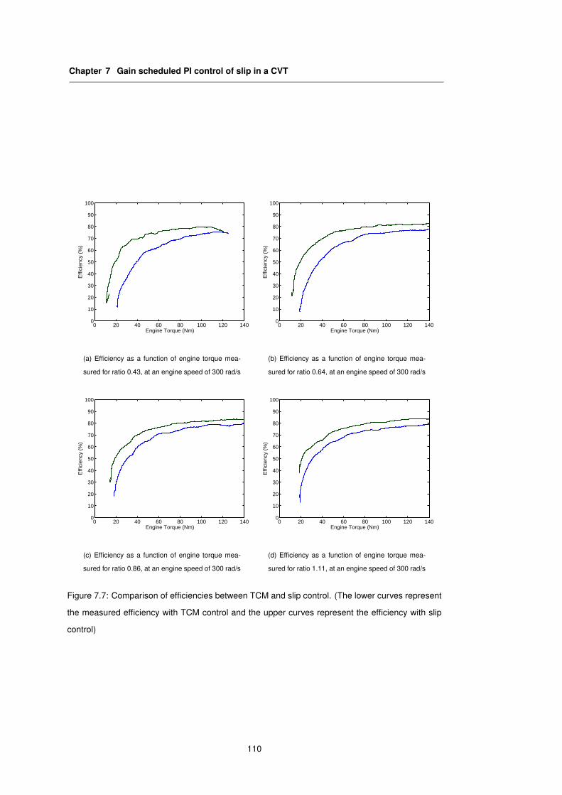
Chapter 7 Gain scheduled PI control of slip in a CVT
0 20 40 60 80 100 120 1400
10
20
30
40
50
60
70
80
90
100
Engine Torque (Nm)
Effi
cien
cy (
%)
(a) Efficiency as a function of engine torque mea-
sured for ratio 0.43, at an engine speed of 300 rad/s
0 20 40 60 80 100 120 1400
10
20
30
40
50
60
70
80
90
100
Engine Torque (Nm)
Effi
cien
cy (
%)
(b) Efficiency as a function of engine torque mea-
sured for ratio 0.64, at an engine speed of 300 rad/s
0 20 40 60 80 100 120 1400
10
20
30
40
50
60
70
80
90
100
Engine Torque (Nm)
Effi
cien
cy (
%)
(c) Efficiency as a function of engine torque mea-
sured for ratio 0.86, at an engine speed of 300 rad/s
0 20 40 60 80 100 120 1400
10
20
30
40
50
60
70
80
90
100
Engine Torque (Nm)
Effi
cien
cy (
%)
(d) Efficiency as a function of engine torque mea-
sured for ratio 1.11, at an engine speed of 300 rad/s
Figure 7.7: Comparison of efficiencies between TCM and slip control. (The lower curves represent
the measured efficiency with TCM control and the upper curves represent the efficiency with slip
control)
110

Chapter 8
Implementation of slip control in aproduction vehicle
The slip control system has been evaluated on two test benches. These test benches are designed
to simulate the driveline of a car, but have certain limitations. One of the limitations is the limited
slope of the torque peaks that can be applied to the variator. In the beltbox testrig, the electric
motors have a higher inertia than a similarly powerful internal combustion engine. This limits the
realism of the tests performed on this testrig. The transmission testrig with the CK2 transmission
uses an internal combustion engine, but has an eddy current brake that is able to simulate road-
loads in normal driving situations, but not torque peaks generated by speed-bumps, slip events,
ABS braking or other specific events requiring very fast transients of the brake torque.
To evaluate a slip controlled CVT under these circumstances a Nissan Primera is used as a test
vehicle [12]. The Nissan Primera driveline is similar to the driveline in the transmission testrig,
but with slight differences which will be explained in Section 8.1. Thereafter the results of the
implementation in the vehicle will be discussed.
8.1. Nissan Primera
The Nissan Primera (shown in Figure 8.1) differs slightly from the testrig setup. The Nissan is
equipped with a 2.3l gasoline engine instead of the 2.0litre engine. Furthermore, the transmission
is a Jatco CK-Kai transmission, which is similar to the CK2 in most aspects, but can handle higher
torques. This is necessary to handle the power from the larger engine.
8.1.1. Engine
The 4 cilinder 2.3litre IC engine has a maximum torque of 234 Nm at 4000 rpm and can deliver
op to 116 kW of power at 5600 rpm. The maximum torque curve is shown in Figure 8.2(b). The
torque output of the engine related to the throttle position has to be known. It is important to know
111

Chapter 8 Implementation of slip control in a production vehicle
Figure 8.1: Picture of the Nissan Primera test vehicle at the Michelin Challenge Bibendum 2006.
the output torque of the engine with a given throttle position and engine speed, since the torque is
not measured between the engine and the transmission.
8.1.2. Transmission control
The transmission control unit of the CK2 transmission uses a Motorola HC12 processor. This
unit controls the ratio and line pressure of the variator and also controls the closing of the torque
converter lock-up clutch. Input signals include the primary and secondary speed, engine speed,
throttle position, ATF temperature and shifter position.
The ratio control strategy is shown in Figure 8.2(a). The aim of the ratio control unit is to minimize
fuel economy while maintaining a good drivability. The ideal line for the 2.0litre engine is shown
in Figure 7.2. The actual strategy for the CK-Kai transmission with the 2.3litre engine is shown in
Figure 8.2(b). If these figures are compared it can be seen that the ratio strategy of the CK-Kai
transmission tries to follow the optimal operation line of the IC engine.
8.1.3. Clamping force control
The clamping force control system based on slip discussed in Chapter 7 is used. The transmission
used on the test bench setup is very similar to the transmission in the test vehicle. Therefore, no
major changes were made to the control system.
112
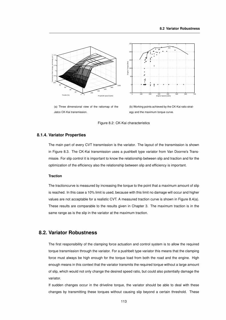
8.2 Variator Robustness
0200
400600
8001000
0
20
40
60
80
1000
0.5
1
1.5
2
2.5
Propshaft speed [rad/s]Throttle [%]
Tra
nsm
issi
on R
atio
\om
ega_
sec/
\om
ega_
pri [
−]
(a) Three dimensional view of the ratiomap of the
Jatco CK-Kai transmission.
0 100 200 300 400 500 600 700−50
0
50
100
150
200
250
Engine Speed [rad/s]
Eng
ine
Tor
que
[Nm
]
(b) Working points achieved by the CK-Kai ratio strat-
egy and the maximum torque curve.
Figure 8.2: CK-Kai characteristics
8.1.4. Variator Properties
The main part of every CVT transmission is the variator. The layout of the transmission is shown
in Figure 8.3. The CK-Kai transmission uses a pushbelt type variator from Van Doorne’s Trans-
missie. For slip control it is important to know the relationship between slip and traction and for the
optimization of the efficiency also the relationship between slip and efficiency is important.
Traction
The tractioncurve is measured by increasing the torque to the point that a maximum amount of slip
is reached. In this case a 10% limit is used, because with this limit no damage will occur and higher
values are not acceptable for a realistic CVT. A measured traction curve is shown in Figure 8.4(a).
These results are comparable to the results given in Chapter 3. The maximum traction is in the
same range as is the slip in the variator at the maximum traction.
8.2. Variator Robustness
The first responsibility of the clamping force actuation and control system is to allow the required
torque transmission through the variator. For a pushbelt type variator this means that the clamping
force must always be high enough for the torque load from both the road and the engine. High
enough means in this context that the variator transmits the required torque without a large amount
of slip, which would not only change the desired speed ratio, but could also potentially damage the
variator.
If sudden changes occur in the driveline torque, the variator should be able to deal with these
changes by transmitting these torques without causing slip beyond a certain threshold. These
113

Chapter 8 Implementation of slip control in a production vehicle
Figure 8.3: Layout of the CK2 transmission
114

8.2 Variator Robustness
−1 0 1 2 3 4 50
0.05
0.1
Slip [%]
Tra
ctio
n [−
]
(a) Traction curve in LOW for the CK2 transmission
−1 0 1 2 3 4 50
0.05
0.1
Slip [%]
Tra
ctio
n [−
]
(b) Traction curve in MED for the CK2 transmission
15 15.5 16 16.5 17 17.5 181000
2000
3000
Rot
atio
nal s
peed
(rp
m)
15 15.5 16 16.5 17 17.5 180
5
10
Slip
(%)
15 15.5 16 16.5 17 17.5 185
10
15
20
Time (s)Cla
mpi
ng F
orce
(kN
)
(c) System response, slip, clamping force and
speeds
0 1 2 3 4 5 60
0.2
0.4
0.6
0.8
1
Slip speed [m/s]
Nor
mal
For
ce [k
N]
(d) F-v diagram
Figure 8.4: Response to torque converter lockup
changes can be caused by the engine or by the road conditions. Focus will therefore be on peaks
in the engine or driveline torque.
Test track results
The vehicle was tested on the Bosch proving grounds in Boxberg, Germany. Over 50 persons drove
the car over a handling course to test the slip controller. These tests showed that under normal
driving conditions the slip controller performed satisfactory. When driving in a more aggressive
way, the slip controller was not always able to keep the slip level within acceptable levels. This
resulted eventually in wear of the belt and pulleys. Figure 8.4 and 8.5 show two major problems
that occurred during the test drive. In these figures both the response of the variator slip to the
event, the clamping force and the shaft speeds are shown as is the F-v diagram for both incidents.
115

Chapter 8 Implementation of slip control in a production vehicle
16 16.5 17 17.5 18 18.5 190.5
11.5
2
Rat
io (
−)
16 16.5 17 17.5 18 18.5 190
10
20
Slip
(%)
16 16.5 17 17.5 18 18.5 190.4
0.6
0.8
Dut
y cy
cle
16 16.5 17 17.5 18 18.5 19
10
20
Time (s)
Cla
mpi
ng F
orce
(kN
)
(a) System response, slip, clamping force and
speeds
0 1 2 3 4 5 60
0.2
0.4
0.6
0.8
1
Slip speed [m/s]
Nor
mal
For
ce [k
N]
(b) F-v diagram
Figure 8.5: Response to a fast downshift
• Closing of the torque converter caused relatively large slip peaks and vibrations in the drive
line. Because the slip controller increases the clamping force with increasing slip, these slip
peaks did not cause damage to the belt and pulleys. The vibrations in the drive line however
cause a very uncomfortable driving experience. Figure 8.4 shows an example of such a
measurement. Opening and closing of the torque converter cause an important change in the
dynamics of the drive train. This effect should be taken into account for further development,
because it can damage the variator as can be seen from the F-v diagram.
• Large slip peaks occurred often with fast variator shifts. This is expected to result from the
assumption that the ratio shifting behavior can be seen as quasi-static. With aggressive driv-
ing this assumption becomes invalid since large and fast downshifts occur with fast variations
of the throttle pedal position. Shifting of the variator can trigger belt slip, as can be seen in
Figure 8.5. Shifting dynamics should therefore be taken into account for future slip control
development. This is especially interesting due to the observation reported by Ide [37], who
found that the shifting dynamics is influenced by variator slip.
8.3. Comfort
Under normal circumstances it should not be possible for the driver to detect whether a CVT is
using slip control or not. The comfort of driving should therefore be the same. Comfort is evaluated
by the driveline shocks introduced or affected by the slip control system.
If the transmission is slipping there is a dampening effect on driveline vibrations due to the decou-
pling of the driveline speed and the engine speed. However, an abrupt slip to stick transition in the
variator creates high torques to synchronize the primary and secondary shaft speeds. This type of
behavior can be felt in the vehicle. These vibrations can be seen in Figure 8.5.
116

8.4 Conclusions and recommendations Nissan Primera tests
For comfort, slip peaks caused by torque peaks from the driveline are less important than slip
caused by engine torque. This is due to the fact that torque peaks from the driveline always cause
shocks in the vehicle. However, torque from the engine should be smoothly transferred to the drive-
shaft to avoid drive discomfort.
During the tests it would occasionally occur that the drive torque from the engine caused slip in the
variator. This could be felt by the driver. This can be caused by a poor engine torque estimation
and by a slow response of the clamping force actuation system.
8.4. Conclusions and recommendations Nissan Primera tests
Unfortunately it was not possible to measure the torques and the fuel consumption in this test ve-
hicle. However, the tests performed with this vehicle were very valuable to evaluate the real life
performance of a CVT with slip control. The tests on the proving ground showed some limitations
to the current implementation of slip control. One of these limitations was the torque induced by
the torque converter lock-up clutch when closing. Also shifting proved a more difficult issue. The
regulation of slip caused also some driveline vibrations that could be felt by the occupants of the car.
117

Chapter 8 Implementation of slip control in a production vehicle
118
Chapter 9
Conclusions and Recommendations
In this chapter conclusions will be drawn, based on this thesis and on the project as a whole.
First, the general conclusions will be given, then some recommendations for future research are
discussed.
9.1. Conclusions
Slip in a variator has long been looked upon as being very destructive to this variator and was to be
avoided at all cost. New findings suggest that a pushbelt type variator can sustain small amounts
of slip for prolonged periods of time without failing or being damaged [89]. With this knowledge in
mind a method is proposed in this thesis to control slip in a variator.
In Chapter 2 several models have been described for the forces acting in the variator. With these
models a fairly accurate prediction can be made for the stationary clamping force ratio in the vari-
ator. The added complexity of the pushbelt model did not give better results compared to the
continuous belt model. For controller design and simulation this model will suffice.
For transient situations the CMM model gave the most accurate result compared to experimental
results. Especially for low transmission ratios the results for the CMM model agreed more with
the experimental results than the other models. In other operating points the Ide model will give
similar results. The Shafai model does not take into account the dependency of the ratio changing
behavior with the input shaft speed as can be seen from the experiments.
In Chapter 3 the traction of the variator was studied. A model of the traction in the variator was
given and the result from this model was compared to measurements. Good agreement was found
for a belt with increased play.
Measurements of the traction coefficient showed that the traction coefficient varies with the relative
slip, ratio, speed and clamping force.
119
Chapter 9 Conclusions and Recommendations
A dynamic model of input speed, slip and transmission ratio in the variator was described in Sec-
tion 3.2. From this model can be derived that the stability of slip in a variator mainly depends on
the slope of the traction curve. If this slope is positive, then slip will be stable. If the slope of the
traction curve is negative, then slip will be unstable.
In Section 3.3 several estimation methods of the geometric ratio and slip were compared. The posi-
tion measurement of the pulley or the belt are accurate enough for estimation of slip and ratio. The
other methods do not work in all required operating points, are not conclusive, or require additional
research.
In Chapter 4 a model was described for the efficiency of the variator. Measurements were used to
identify the torque loss in the variator. Using this torque loss an accurate prediction can be made
for the efficiency of the variator.
From the measurements of the efficiency for different geometric ratios can be seen that the effi-
ciency of the variator near rg = 1 is higher than the efficiency in other ratios. This is caused by the
absence of slip between bands and blocks in the belt.
The measurements of the efficiency of the variator showed that the optimal operating point of the
variator is at a slip level higher than zero. If the efficiency curve is compared to the traction curve,
than it can be seen that the optimal efficiency point is reached before the maximum of the traction
coefficient is reached if slip is increased. However, if the actuation losses of a hydraulic system is
taken into account the slip level of the optimal efficiency is very near the slip level of the maximum
traction coefficient. This means that if the variator is operated at its maximum efficiency, the safety
margin is almost zero.
In Chapter 5 the clamping force control problem is discussed. In the case of classic clamping
force control methods only open-loop control is used. If slip control is used, the feedback loop can
be used to stabilize the variator in operating points that would be unstable with the open-loop con-
trol. The simulation results showed that open-loop clamping force control is vulnerable for torque
peaks caused by extreme events except for very high safety-factors. High safety-factors will reduce
the efficiency of the variator as described in Chapter 4.
In Chapter 6 the results were shown of the first implementation of slip control in a pushbelt type vari-
ator. The test results showed promising results. The setup used however a far more sophisticated
actuation system than the actuation systems used in production CVTs. Therefore an implementa-
tion is done on the CK2 transmission described in Chapter 7. In this chapter a slip control algorithm
is tested in a production CVT. Slip control was implemented and tested in a test facility with an
internal combustion engine simulating a complete driveline of a Nissan Primera. Although the tests
were successful, they proved not completely conclusive, because of the limitations of the testrig.
120

9.2 Recommendations
Therefore slip control was implemented in a test vehicle, a Nissan Primera. The results from these
tests were shown in Chapter 8. Several complications were found with the implementation in the
Nissan Primera.
Important factors for successful implementation of slip control are:
• the bandwidth of the actuation system,
• quality of the measured slip signal,
• quality of the estimation of the road-load and the engine torque.
The improvements that can be reached using slip control in a CVT:
• 50% less clamping force compared to the CK2 transmission,
• Over 30% improvement in efficiency at low ratios and low torques,
• Around 5% improvement in efficiency at higher ratios and higher torques.
9.2. Recommendations
For further research a few suggestions are given to extend the knowledge gained in this project.
• The ratio changing behavior of the variator, especially under macro-slip conditions is not well
known. This should be investigated further, because a slip controlled variator can have very
different ratio changing dynamics when the reference value of slip is in the macro-slip area.
The closed loop system might become unstable, because the ratio changing dynamics will
change.
• To be able to use beltspeed for the estimation of slip or ratio, it is necessary to know on which
pulley slip will occur. Measurements of the beltspeed combined with the pulley position can
give this insight. This knowledge can also be helpful for improving the model of beltslip.
• To be able to estimate the geometric ratio or slip without adding extra sensors to the variator
would make slip control more interesting for commercialization. Some methods are proposed
in this thesis, but more research on this topic is necessary for useful results.
• To improve the efficiency of the pushbelt type variator a pushbelt should be developed with-
out a difference in running radius between the bands and blocks, eliminating the friction in
121
Chapter 9 Conclusions and Recommendations
the belt.
• The durability of the variator under slip control was not investigated. It would be of interest to
know the consequences of slip control with respect to durability.
• The performance of the system could unfortunately not be tested for several drive cycles like
the NEDC. This was due to the limitations of the test setups. It will be valuable to perform
this test in future research.
• In Appendix A a decoupling and linearizing feedback is proposed to include the ratio changing
behavior of the variator in the controller. With this method the influences of the nonlinearities
and the coupling between ratio and clamping force control might be reduced significantly.
This could potentially make the design of a controller for either the ratio or clamping force
easier.
122
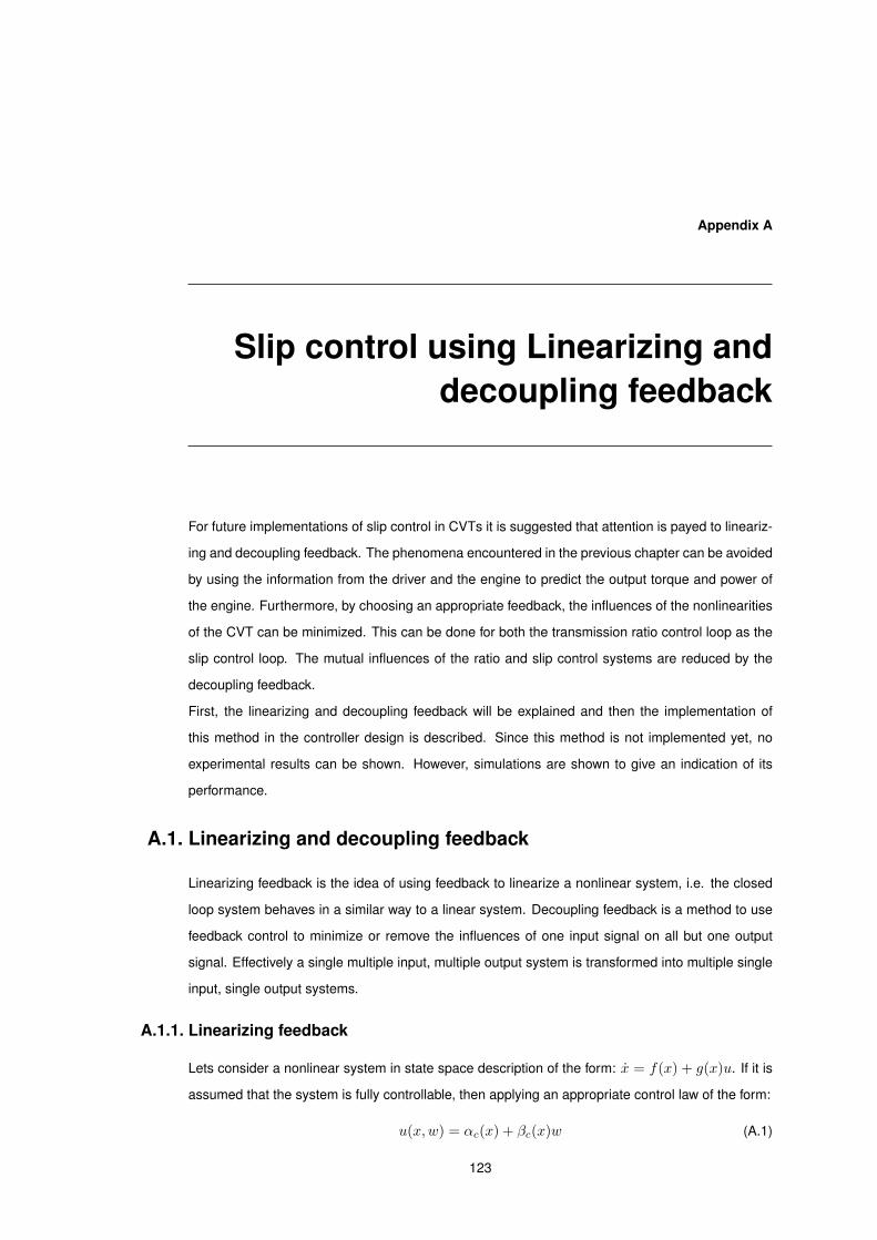
Appendix A
Slip control using Linearizing anddecoupling feedback
For future implementations of slip control in CVTs it is suggested that attention is payed to lineariz-
ing and decoupling feedback. The phenomena encountered in the previous chapter can be avoided
by using the information from the driver and the engine to predict the output torque and power of
the engine. Furthermore, by choosing an appropriate feedback, the influences of the nonlinearities
of the CVT can be minimized. This can be done for both the transmission ratio control loop as the
slip control loop. The mutual influences of the ratio and slip control systems are reduced by the
decoupling feedback.
First, the linearizing and decoupling feedback will be explained and then the implementation of
this method in the controller design is described. Since this method is not implemented yet, no
experimental results can be shown. However, simulations are shown to give an indication of its
performance.
A.1. Linearizing and decoupling feedback
Linearizing feedback is the idea of using feedback to linearize a nonlinear system, i.e. the closed
loop system behaves in a similar way to a linear system. Decoupling feedback is a method to use
feedback control to minimize or remove the influences of one input signal on all but one output
signal. Effectively a single multiple input, multiple output system is transformed into multiple single
input, single output systems.
A.1.1. Linearizing feedback
Lets consider a nonlinear system in state space description of the form: x = f(x) + g(x)u. If it is
assumed that the system is fully controllable, then applying an appropriate control law of the form:
u(x,w) = αc(x) + βc(x)w (A.1)
123

Appendix A Slip control using Linearizing and decoupling feedback
makes the system linear with respect to the new control input w, so that linear control methods can
be used to regulate this system [39].
A.1.2. Decoupling feedback
Decoupling state feedback was introduced by Gilbert [32]. A system is considered with two inputs
and two states. If this system is linear, then the following state space description can be obtained:⎡⎣ x1
x2
⎤⎦ =
⎡⎣ a11 a12
a21 a22
⎤⎦
⎡⎣ x1
x2
⎤⎦ +
⎡⎣ b11 b12
b21 b22
⎤⎦
⎡⎣ u1
u2
⎤⎦ (A.2)
If the diagonal terms of a12 and a21 and/or b12 and b21 are not zero then the input u1 has influence
on both x1 and x2. If an appropriate control law of the form:⎡⎣ u1
u2
⎤⎦ = −
⎡⎣ a12
b11x2
a21b22
x1
⎤⎦ −
⎡⎣ b12
b11u2
b21b22
u1
⎤⎦ +
⎡⎣ w1
w2
⎤⎦ (A.3)
is applied, so that the influence of w1 on x2 is zero, then effectively a decoupled system is obtained
of the form: ⎡⎣ x1
x2
⎤⎦ =
⎡⎣ a11 0
0 a22
⎤⎦
⎡⎣ x1
x2
⎤⎦ +
⎡⎣ b11 0
0 b22
⎤⎦
⎡⎣ w1
w2
⎤⎦ (A.4)
This method can in certain situations be extended to nonlinear applications. Modeling uncertainties
and measurement errors reduce the decoupling effect.
A.2. Controller design
In the previous chapters the control design was based on the assumption that the ratio chang-
ing is quasi-static. If the ratio changing is not quasi-static, the control problem becomes more
complicated, because of the interactions between the ratio dynamics and the slip dynamics. If a
decoupling and linearizing feedback can be designed, the control design can be simplified. The
ratio control has no longer an influence on the slip dynamics and vice versa. Linear control design
techniques can be used.
If we assume that Fs is smaller than Fp, ωp and ωs are measured, an estimate exists for the geo-
metric ratio, rg, and that estimates Te, Td are available for the disturbances, control inputs Fp and
Fs can be chosen such that for inputs u1 and u2 an almost linear system with respect to rg and ν,
the controlled variables, is found.
Therefore a control law should be designed such that:
1. the slip ν, with unknown initial error, converges as fast as possible to a prescribed (constant)
value νd and
2. the ratio rg converges as fast as possible to the prescribed value rd.
124

A.2 Conclusions and recommendations linearizing and decoupling feedback
C
G2s G1sActuator dynamics Variator slip dynamics
p
ref
rg
Te, Td
-+ e
us F
G2r G1rNonlinear Controller Actuator dynamics Variator ratio changing
dynamics
rref
Plant
-+ er ur
rg
Variator
Te, Td^ ^
Figure A.1: Block diagram of the variator control scheme
To meet the second demand, we choose:
ln(
Fp
ΨFs
)=
1ωpκ(rg)
(rd + u1) (A.5)
with a new input u1. With this choice follows:
rg − rd = u1 (A.6)
To meet the first demand we choose:
2μ(ν, rg)Rs(rg)cos β
Je + (1 − ν)r2gJs
JeJsFs = (1−ν)ωp(rd+u1)+(1−ν)
rg
JeTe+
1Js
Td−u2rgωp (A.7)
With this new input u2 follows:
ωprg ν = ωprgu2 + (1 − ν)rg
Je(Te − Te) +
1Js
(Td − Td) (A.8)
Reconstructing the variator inputs Fp and Fs from these control inputs gives:
Fs =cos β
2μRs
JeJs
Je + (1 − ν)r2gJs
[(1 − ν)(ωprd + rg
Te
Je) +
Td
Js+ ((1 − ν)u1 − rgu2) ωp
]
Fp = ΨFserd+u1
ωpκ(rg)
For the situation that Fp < Fs a solution can be found in a similar way.
The first order differential equation with x = [ωp, ν, rg]T is now given by:
x =
⎡⎢⎢⎢⎣
Te
Je− Js
Je+(1−ν)r2gJs
[(1 − ν)(ωprd + rg
Te
Je) + Td
Js+ ((1 − ν)u1 − rgu2)ωp
]u2 + (1 − ν) 1
Jeωp(Te − Te) + 1
ωprgJs(Td − Td)
u1 + rd
⎤⎥⎥⎥⎦
125

Appendix A Slip control using Linearizing and decoupling feedback
As output is chosen:
y =
⎡⎢⎢⎢⎣
ωp
ν
rg
⎤⎥⎥⎥⎦ (A.9)
Both inputs are independent and have a linear relation to the controlled variable. Using linear
control techniques a suitable controller can be designed for u1 and u2.
A.3. Conclusions and recommendations linearizing and decouplingfeedback
In this chapter a linearizing and decoupling feedback has been designed. This feedback method
can be used to minimize the influences of the ratio control on the slip control system and vice
versa. It should improve the effectiveness of the slip control system. However, further investigation
is necessary into the feasibility and possibilities of the method. So far, no tests have been done with
this control strategy. For the successful implementation of this method the modeling uncertainties
should not be too large and the estimations of the disturbances, Td and Te, must be reasonably
accurate.
126

Appendix B
Equations
B.1. System matrices for the linearized model
The derivatives Dp of the primary radius Rp and Ds of the secondary radius Rs with respect to the
ratio rg can be determined from the geometric relations in Chapter 2. If the elongation of the belt
is neglected it follows that:
Dp(rg) =d
drg(Rp(rg)) =
π − 2φ(rg)(π − 2φ(rg)) + (π + 2φ(rg))rg
· Rp(rg)rg
(B.1)
Ds(rg) =d
drg(Rs(rg)) =
π + 2φ(rg)(π − 2φ(rg)) + (π + 2φ(rg))rg
· Rs(rg) (B.2)
With respect to the experimentally determined functions μ = μ(ν, rg), Ψ = Ψ(ν, rg) and κ =
κ(ν, rg) it is assumed that they are continuous and at least once differentiable with continuous
partial derivatives, i.e.
Mν(ν, rg) =∂
∂ν(μ(ν, rg)); Mr(ν, rg) =
∂
∂rg(μ(ν, rg)) (B.3)
Pν(ν, rg) =∂
∂ν(Ψ(ν, rg)); Pr(ν, rg) =
∂
∂rg(Ψ(ν, rg)) (B.4)
Kν(ν, rg) =∂
∂ν(κ(ν, rg)); Kr(ν, rg) =
∂
∂rg(κ(ν, rg)) (B.5)
With these derivatives the system equations, given by (see Section 3.2:
x = f(x, u) + L(x)w, (B.6)
can be linearized around a stationary working point, characterized by the state x0, the input u0 and
the disturbance w0. In state space the result can be written as:
δx = A0δx + B0δu + L0δw (B.7)
where the state matrix A0 and the input matrix B0 follow from:
A0 = A(x0, u0); A(x, u) =∂
∂xT(f(x, u) (B.8)
127

Appendix B Equations
B0 = B(x0, u0); B(x, u) =∂
∂uT(f(x, u) (B.9)
whereas the disturbance matrix L0 is given by:
L0 = L(x0) (B.10)
With x = [ωp, ωs, rg]T , u = [Fp, Fs]T and w = [Te, Td]T the matrices are found to be:
A0 =2F0
cos β
⎡⎢⎢⎢⎣
−Rs0k1irs0Jeωp0
Rs0k1iJeωp0
−Rs0(k1i+k2i)Je
Rs0k1irs0Jsωp0rg0
− Rs0k1iJsωp0rg0
−Rs0k1iωs0Jsωp0r2
g0
cos βκ0 log(Fp
ΨFs)
2F00 0
⎤⎥⎥⎥⎦ (B.11)
B0 =
⎡⎢⎢⎣
− 2Rp0μ
Je cos β0
0 2Rs0μJs cos β
κ0ωp0Fs
κ0ωp0Fp
⎤⎥⎥⎦ (B.12)
L0 =
⎡⎢⎢⎣
1Je
0
0 − 1Js
0 0
⎤⎥⎥⎦ (B.13)
B.2. Iterative calculation of the wrapped angle and running radii
For calculating the wrapped angle of the belt on the pulley φ must be known. The relation be-
tween the running radii and the wrapped angle are implicit. The following algorithm can be used to
calculate the value of φ using an iterative procedure for a given transmission ratio rg.
L = Rp(π + 2φ) + Rs(π − 2φ) + 2a cos φ (B.14)
Rp − Rs = a sin φ (B.15)
rg =Rp
Rs(B.16)
ρg =1 − rg
1 + rg(B.17)
Using Equations B.16 and B.17 we can rewrite Equation (B.14) to:
f(φ) = (π
2+ ρgφ) sinφ + ρg cos φ − ρg
L
2a(B.18)
f(φ) = 0 (B.19)
Differentiating f(φ) with respect to φ gives:
f ′(φ) = (π
2+ ρgφ) cos φ (B.20)
If φi is a reasonable estimation of the zero of f(φ), then a new approximation φi+1 can be deter-
mined by:
φi+1 = φi − f(φi)f ′(φi)
(B.21)
128

B.3 Quadratic approximation of the wrapped angle and running radii
If this iteration is stopped when∣∣∣ f(φi)f ′(φi)
∣∣∣ < ε, then a solution has been found that has a relative
error smaller than ε. Using Equations B.14 and B.16 also the values for Rp and Rs can be found.
B.3. Quadratic approximation of the wrapped angle and running radii
Equations (B.14) and (B.16) can be approximated with a quadratic function using the second order
Taylor expansion of the cosine and sine functions:
cos φ ≈ 1 − 12φ2 (B.22)
sin φ ≈ φ (B.23)
Rewriting Equation (B.14) gives:
L = Rp
(π + 2
Rp − Rs
a
)+ Rs
(π − 2
Rp − Rs
a
)+ 2a
(1 − 1
2
(Rp − Rs
a
)2)
φ =Rp − Rs
a(B.24)
This equation can be solved if the ratio rg is known or one of the running radii is known. Using
Equation (B.24) the wrapped angles can be calculated.
129

Appendix B Equations
130

Appendix C
Robust PI Control
Panagopoulos [61], [60] and Solyom [76] proposed a method for PI controller synthesis with certain
robustness properties which minimizes the effect of a load disturbance by maximizing the integral
gain. The closed-loop stability is guaranteed by two constraints posed on the system. They showed
this method for a class of systems with a cone bounded nonlinearity in the control loop.
For optimal load disturbance attenuation, the maximum value of the integral gain is determined
from the figure. The proportional gain is then determined graphically.
The PI control synthesis problem can be seen as the following optimization problem:
max ki
subjectto f(kp, ki, ω1) ≥ R2s ∀ ω1 > 0 (C.1)
g(kp, ki, ω2) ≥ 0 ∀ ω2 > 0 (C.2)
kp > 0, ki > 0 (C.3)
Constraints (C.1) and (C.2) can be plotted as ellipses in the kp-ki plane. In this way the optimization
problem can be visualized using this graphical representation. The graphical representation is
shown in Figure C.1.
Constraint (C.1) is the function:
f(kp, ki, ω1) = |Cs + C(iω)G(iω)|2 (C.4)
By choosing Rs and Cs = 1 the controller will have a maximum closed loop sensitivity of 1/Rs.
This is called the sensitivity constraint.
Constraint (C.2) is called the robustness constraint. This constraint guarantees the stability of
the closed loop system for all systems within the uncertainty bounds. With the closed loop plant
P = G1(s)/(1 + C(s)G1(s)G2(s)), where G1(s) is the linear plant and G2(s) is the nonlinear
feedback, the robustness constraint can be written as:
Re{
1 + βP (iω)1 + αP (iω)
}> 0 (C.5)
131

Appendix C Robust PI Control
−0.5 0 0.5 1 1.5 2 2.5 30
0.1
0.2
0.3
0.4
0.5
0.6
0.7
0.8
0.9
1
kp
k i
Figure C.1: Combined criteria
In this equation α and β are the uncertainties parameters of the (unknown) nonlinearity.
Constraint (C.3) further guarantees that the controller does not have unstable zeros. For proofs is
referred to Solyom [75].
132

Appendix D
Drive cycles
It is very difficult to compare vehicles in terms of fuel economy and emissions on the basis of
real world driving. Field tests are not reproducible and als measured real life driving situations
are mostly to dynamic to reproduce in a laboratory. Therefore standardized drive cycles are used.
For measurement purposes easy to follow drive cycles are used like the NEDC cycle [19] and for
simulation purposes also more complex drive cycles can be used. For comparison reasons it is
useful if results can be compared on the basis of standardized cycles. The type of drive cycle has
a large influence on the performance of a drivetrain. Therefore several drive cycles are compared
and their advantages and disadvantages are discussed.
D.1. NEDC
The New European Drive Cycle combines three city cycles with one highway cycle. This cycle is
not a very realistic drive cycle, because it contains several constant velocity parts and constant
acceleration parts, but it can be reproduced in experiments. Other cycles, for example cycles mea-
sured in real traffic, are very difficult or almost impossible to reproduce accurately. Therefore the
NEDC drive cycle is ideal for laboratory testing of a car.
The NEDC cycle is plotted in Figure D.1(a). The required accelerations are plotted in Figure D.1(c).
The accelerations are more or less constant, but are realistic for real driving. For a midsize car
a histogram of the power needed to run the NEDC cycle is plotted in Figure D.1(e). From these
figures can be seen that the power needed for this cycle is relatively low.
Drivetrain concepts that are optimized for partload conditions will perform much better than tradi-
tional drivetrain concepts. Furthermore, from Figure D.1(a) can be seen that a lot of the cycle the
vehicle is standing still. This is an advantage for concepts that use a start-stop strategy.
133
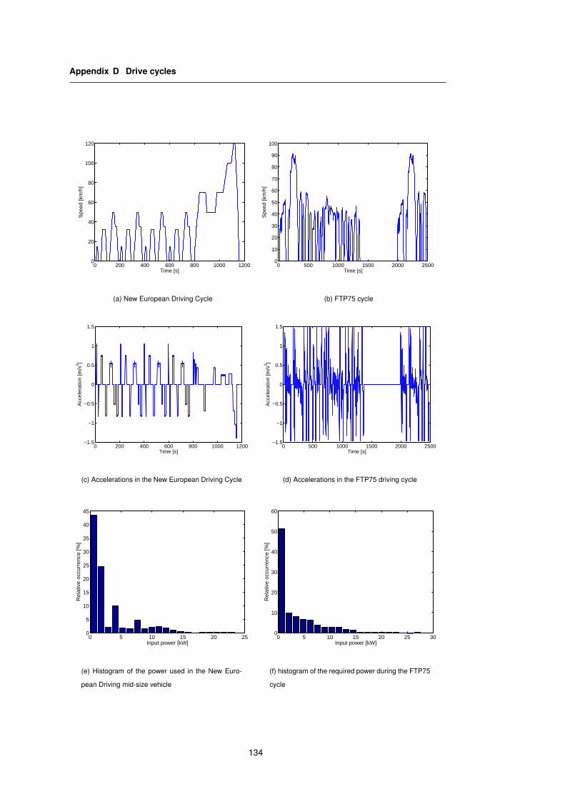
Appendix D Drive cycles
0 200 400 600 800 1000 12000
20
40
60
80
100
120
Time [s]
Spe
ed [k
m/h
]
(a) New European Driving Cycle
0 500 1000 1500 2000 25000
10
20
30
40
50
60
70
80
90
100
Time [s]S
peed
[km
/h]
(b) FTP75 cycle
0 200 400 600 800 1000 1200−1.5
−1
−0.5
0
0.5
1
1.5
Time [s]
Acc
eler
atio
n [m
/s2 ]
(c) Accelerations in the New European Driving Cycle
0 500 1000 1500 2000 2500−1.5
−1
−0.5
0
0.5
1
1.5
Time [s]
Acc
eler
atio
n [m
/s2 ]
(d) Accelerations in the FTP75 driving cycle
0 5 10 15 20 250
5
10
15
20
25
30
35
40
45
Input power [kW]
Rel
ativ
e oc
curr
ence
[%]
(e) Histogram of the power used in the New Euro-
pean Driving mid-size vehicle
0 5 10 15 20 25 300
10
20
30
40
50
60
Input power [kW]
Rel
ativ
e oc
curr
ence
[%]
(f) histogram of the required power during the FTP75
cycle
134

D.2 FTP75
D.2. FTP75
The FTP75 cycle [28] is the official driving cycle of the US federal government. FTP stands for
Federal Test Procedure and is used for fuel economy and emission testing. The FTP75 cycle is
more dynamic than the NEDC cycle. This cycle is used for simulation of drivetrain performance in
city and rural road traffic and is mostly used in the USA. High speeds are not reached. The FTP75
cycle is plotted in Figure D.1(b).
In Figure D.1(d) the accelerations are shown for the FTP75 drivecycle. From this graph can be seen
that the accelerations are about 1.5 times higher than the accelerations in the NEDC cycle. This
results in more required power needed to drive the cycle with the same automobile. However, the
FTP75 cycle has a relatively long standing still period. This means that the overall dependence of
the total fuel economy on the higher loads is small. In Figure D.1(f) gives the relative occurrences
of different loads during the cycle.
135

Appendix D Drive cycles
136
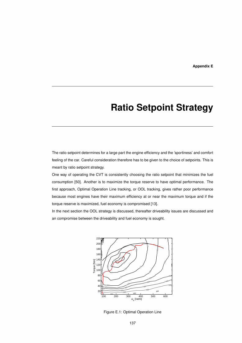
Appendix E
Ratio Setpoint Strategy
The ratio setpoint determines for a large part the engine efficiency and the ’sportiness’ and comfort
feeling of the car. Careful consideration therefore has to be given to the choice of setpoints. This is
meant by ratio setpoint strategy.
One way of operating the CVT is consistently choosing the ratio setpoint that minimizes the fuel
consumption [50]. Another is to maximize the torque reserve to have optimal performance. The
first approach, Optimal Operation Line tracking, or OOL tracking, gives rather poor performance
because most engines have their maximum efficiency at or near the maximum torque and if the
torque reserve is maximized, fuel economy is compromised [13].
In the next section the OOL strategy is discussed, thereafter driveability issues are discussed and
an compromise between the driveability and fuel economy is sought.
245
250
250
250
250
260
260
260
260
260
275
275
275
275
275
275
300
300
300
300
300
325
325
325
325
325350 350
350
350
400
400
400
500500
500
800 800800
ωe [rad/s]
Tor
que
[Nm
]
100 200 300 400 500 600
20
40
60
80
100
120
140
160
180
200
220
Figure E.1: Optimal Operation Line
137

Appendix E Ratio Setpoint Strategy
E.1. Optimal Operation Line
OOL tracking is the most fuel economical way to operate the driveline. The OOL as shown in
Figure E.1 can be calculated from the engine map by minimizing the fuel consumption in g/kWh
for a set of output power values. For a given output power setting the relation between the engine
torque en the engine speed is given by:
Tengine =Prequired
ωengine(E.1)
On this iso-power curve the point with the minimum fuel consumption per unit of energy is taken. If
this process is repeated for a set of possible power settings, each giving one point on the OOL, an
estimate of the OOL is found.
The torque output of the engine is not linear with the throttle position. Because the torque of the
engine is not known, but the throttle position is, the throttlemap is used to estimate the torque output
of the engine. This throttlemap is shown in Figure E.2.
Using this throttlemap and the OOL, a ratio control strategy can be derived by:
r(xthrottle, ωdriveshaft) (E.2)
The OOL can be approximated using a third order polynomial. The result is shown in Figure E.3.
The smoothing of the OOL improves the smoothness of the shifting and decreases the number of
datapoints in the embedded controller. On the other hand it will increase the fuel consumption of
the vehicle.
E.2. Drivability
From the OOL the optimal engine speed for a give throttle position can be obtained. If this strategy is
used, the drivability of the vehicle is lowered, because the response to sudden throttle movements
is slow. Since drivability is also an important issue for ratio control design, a new line has to be
designed that finds a good combination of fuel economy and drivability. In this paper drivability
will be evaluated using simulation [34]. The ratio control strategy is evaluated for fuel economy,
acceleration times of 0-100, 50-80 and 80-120.
A cost function is designed that is minimized:
J = lfuelγ1 + t0−100γ2 + t50−80γ3 + t80−120γ4 + aminγ5 + amaxγ6 (E.3)
In this equation γ1−6 are the weighting factors for the different measurement values.
The NEDC cycle is used to evaluate the fuel economy [97], acceleration simulations are used to
evaluate the drivability.
The fuel consumption map of the IC engine used is defined for a certain torque/engine speed com-
bination. To obtain the relation of the engine torque with the throttle position the map in Figure E.2
138

E.2 Drivability
150 200 250 300 350 400 450 500 550 6000
50
100
150
200
250
Engine speed [rad/s]
Tor
que
[Nm
]
0
6.25
12.5
25
37.5
50
62.5
75
87.5
100
Figure E.2: Throttle map
0 20 40 60 80 1000
100
200
300
400
500
600
ωe [r
ad/s
]
Throttle [%]
OOL (optimal operation line)Approximation of OOLRatio strategy based on OOL
Figure E.3: Optimal Operation Line strategy compared to approximated OOL lines
0
50
1000500
10001500
0
1
2
3
ωs [rad/s]Throttle [%]
Rat
io [−
]
Figure E.4: Optimal Operation Line
139

Appendix E Ratio Setpoint Strategy
is used.
The ratio control strategy can be calculated from:
ωengine = f (xthrottle, ωdriveshaft) (E.4)
The engine speedmap gives a function of the throttle position and the driveshaft speed. For the
OOL tracking this would look like the solid line in Figure E.1.
An alternative line is designed using the following method:
ωengine = min (ωmax, max (ωmin, f (xthrottle, ωdriveshaft))) (E.5)
Where f (xthrottle, ωdriveshaft) is a third order approximation of the Optimal Operation Line (OOL).
A factor is added to increase the torque reserve of the engine, thereby increasing the responsive-
ness of the vehicle. This value is of course a compromise between agility and fuel consumption.
Furthermore, the engine speed is increased with increasing driveshaft speed to enhance the feel-
ing of the driver. The amount with which this is done is given by: ωd2.
Three variables are subject to tuning: [ωd1, ωd2, ωd3].
Dynamic programming is used to determine the best compromise. For all possible values of the
design variables a simulation is done and the results are used to calculate the cost of each combi-
nation of the design variables [7].
Implementation is done by calculating a 2D lookup table of desired ratios for each vehicle speed
and throttle position combination. This is stored in a matrix in the TCM.
Because of several reasons mentioned earlier a stepped ratio approach is investigated. For each
of the possible combinations of the design variables also a stepped ratio control strategy is derived.
For this purpose the continuous ratio strategy as stored in the 2D lookup table is quantized in a
fixed number of evenly distributed steps.
System constraints are:
RATIO
minimum ratio: (LOW) 0.45
maximum ratio: (OD) 2.25
ENGINE SPEED
minimum engine speed: 80 rad/s
maximum engine speed: 550 rad/s
E.2.1. Shiftspeed
The reference of the transmission ratio from the ratio strategy can change as fast as the movement
of the gaspedal. If the ratio of the CVT would change this fast very nervous drivetrain behavior
140

E.2 Drivability
0.45
0.450.45
0.59
0.59
0.59
0.77
0.77
0.77
1
1
1
1
1.31
1.31
1.31
1.31
1.7
1.7
1.7
1.7
2.23
2.23
2.23
2.23
ωs [r
ad/s
]
Throttle [%]0 20 40 60 80 100
0
200
400
600
800
1000
1200
Figure E.5: CVT Ratio control strategy
0.45
0.450.45
0.59
0.59
0.59
0.77
0.77
0.77
1
1
1
1
1.31
1.31
1.31
1.7
1.7
1.7
1.7
2.23
2.23
2.23
2.23
ωs [r
ad/s
]
Throttle [%]0 20 40 60 80 100
0
200
400
600
800
1000
1200
Figure E.6: CVT Ratio control strategy based on the Optimal Operation Line
141

Appendix E Ratio Setpoint Strategy
would result. Moreover, due to inertial effects unwanted accelerations would occur. These effects
are detrimental to the driving experience.
To avoid the nervous behavior of the variator, the reference value can be filtered. Another approach
is to apply a rate-limiter. Because the variator behaves like a first order system (see Chapter 3) the
latter can be used without problems.
142

Bibliography
[1] S. Akehurst, N.D. Vaughan, D.A. Parker, and D. Simner. Modelling of loss mechanisms in a
pushing metal V-belt continuously variable transmission. part 1: torque losses due to band
friction. Proc. Instn Mech. Engrs Vol. 218 Part D: J. Automobile Engineering, pages 1269–
1281, 2004.
[2] S. Akehurst, N.D. Vaughan, D.A. Parker, and D. Simner. Modelling of loss mechanisms in
a pushing metal V-belt continuously variable transmission. part 2: pulley deflection losses
and total torque loss validation. Proc. Inst. Mech. Engineers Vol. 218 Part D: J. Automobile
Engineering, pages 1283–1293, 2004.
[3] S. Akehurst, N.D. Vaughan, D.A. Parker, and D. Simner. Modelling of loss mechanisms in a
pushing metal V-belt continuously variable transmission. part 3: belt slip losses. Proc. Inst.
Mech. Engineers Vol. 218 Part D: J. Automobile Engineering, pages 1295–1306, 2004.
[4] G. Amontons. De le resistance causee dans les machines. Memoires de lAcademie des
Sciences, pages 203–222, 1699.
[5] H. Asayama, J. Kawai, A. Tonohata, and M. Adachi. Mechanism of metal pushing belt. JSAE
Review 16, pages 137–143, 1995.
[6] B. Bertsche, H. Naunheimer, and G. Lechner. Fahrzeuggetriebe. Springer-Verlag, 1994.
[7] D.P. Bertsekas. Dynamic programming and optimal control. Athena Scientific, Massachusetts,
1995.
[8] B. Bonsen, C. de Metsenaere, T.W.G.L. Klaassen, K.G.O. van de Meerakker, P.A. Veenhuizen,
and M. Steinbuch. Simulation and control of slip in a continuously variable transmission. In
Advanced Vehicle Control (AVEC), 2004.
[9] B. Bonsen, T.W.G.L. Klaassen, R.J. Pulles, S.W.H. Simons, M. Steinbuch, and P.A. Veen-
huizen. Performance optimization of the push-belt CVT by variator slip control. Int. J. of
Vehicle Design, 39(3):232–256, 2005.
143

Bibliography
[10] B. Bonsen, T.W.G.L. Klaassen, K.G.O. van de Meerakker, M. Steinbuch, and P. Veenhuizen.
Analysis of slip in a continuously variable transmission. IMECE Congress and RD&D Expo
2003, 2003.
[11] B. Bonsen, T.W.G.L. Klaassen, K.G.O. van de Meerakker, M. Steinbuch, and P.A. Veenhuizen.
Measurement and control of slip in a continuously variable transmission. IFAC Mechatronics
2004, 2004.
[12] B. Bonsen, R. J. Pulles, S.W.H. Simons, M. Steinbuch, and P. A. Veenhuizen. CVT slip control
implementation in a production vehicle. IEEE Conference on Control Applications, 2005.
[13] B. Bonsen, P.A. Veenhuizen, and M. Steinbuch. CVT ratio control strategy optimization. Pro-
ceedings of the Conference on Vehicle Power and Propulsion (VPP’05), 2005.
[14] E. Buckingham. On physically similar systems: Illustrations of the use of dimensional equa-
tions. Phys. Rev., 4:345–376, 1914.
[15] E. Buckingham. Model experiments and the form of empirical equations. Trans. ASME,
37:263, 1915.
[16] E. Buckingham. The principle of similitude. Nature, 96:396–397, 1915.
[17] G. Carbone, L. Mangialardi, B. Bonsen, C. Tusi, and P.A. Veenhuizen. CVT dynamics: Theory
and experiments. International Journal of Mechanism and Machine Theory, 2006.
[18] G. Carbone, L. Mangialardi, and G. Mantriota. The influence of pulley deformations on the
shifting mechanism of metal belt CVT. Journal of Mechanical Design, 2004.
[19] European Committee. EEC Directive 90/C81/01 emission test cycles for the certification of
light duty vehicles in Europe, Brussels, 2001.
[20] C.A. Coulomb. Theorie des machines simples. Memoires de Mathematique et de Physique
de lAcademie ds Sciences, pages 161–331, 1785.
[21] Leonardo da Vinci. Studies of friction. ca 1513-1514.
[22] C. de Metsenaere, B. Bonsen, and P.A. Veenhuizen. Survey into CVT slip control potential
using matlab R©/simulink R© simulation. Technical Report DCT 2004-76, TU Eindhoven, 2004.
[23] C. Canudas de Wit, P. Tsiotras, X. Claeys, J. Yi, and R. Horowitz. Nonlinear and Hybrid
Systems in Automotive Control, chapter Friction Tire/Road Modeling, Estimation and Optimal
Braking Control, pages 147–210. Springer, 2003.
[24] Van Doorne. dr. Hub J. van Doorne. 2000.
[25] R.G.J. Drabbels, B. Bonsen, and N.J.J. Liebrand. Traction curve measurements with controlled
ratio. Technical Report DCT 2004.22, TU Eindhoven, 2004.
144

[26] S. Drakunov, U. Ozguner, P. Dix, and B. Ashrafi. ABS control using optimum search via sliding
modes. Proceedings of the 33rd conference on decision and control (CDC), pages 466–471,
1994.
[27] dSpace. dspace R©. Website.
[28] EPA. Motor vehicle emissions federal test procedure revisions; final regulations. Website,
1996.
[29] J.A. Eytelwein. Handbuch der Statik fester Korper. Reiner Berlin, 1808.
[30] H. Faust, M. Homm, and F. Bitzer. Wirkungsgradoptimiertes CVT-Anpresssystem. 7. LuK
Kolloquium 2002, pages 61–73, 2002.
[31] G. Gerbert. Mechanism of a metal V-belt. ASME paper no. 84-DET-227, 1984.
[32] E.G. Gilbert. The decoupling of multivariable systems by state feedback. SIAM Journal of
Control, 7:50–63, 1969.
[33] Hitachi. Hybrid electric vehicle electric oil pump motor for CVT transmission. Website.
[34] T. Hofman and R.M. van Druten. Research overview: Design specifications for hybrid vehicles.
in European ELE-DRIVE Transportation; Editors: AVERE, Lissabon, 2004.
[35] T. Ide. Effect of power losses of metal V-belt CVT components on the fuel economy. Int.
Congress on Continuously Variable Power Transmimssion, pages 93–98, 1999.
[36] T. Ide, H. Uchiyama, and R. Kataoka. A dynamic response analysis of a vehicle with a metal
V-belt CVT. Proceedings of AVEC’94, 1994.
[37] T. Ide, H. Uchiyama, and R. Kataoka. Experimental investigation on shift-speed characteristics
of a metal V-belt CVT. In Proc. of the 1st IFAC Workshop on Advances in Automotive Control,
pages 99–107, 1996.
[38] N. Indlekofer, U. Wagner, A. Fidlin, and A. Teubert. Latest results in the CVT development.
7th LuK Symposium, pages 51–60, 2002.
[39] A. Isidori. Nonlinear control systems. 1989.
[40] Jatco. www.jatco.co.jp. Website, 2005.
[41] U. Kiencke and L. Nielsen. Automotive Control Systems, chapter ABS Control Systems, pages
409–414. Springer, 2005.
[42] H. Kim and J. Lee. Analysis of belt behavior and slip characteristics for a metal V-belt CVT.
Mechanics and Machine Theory, Vol 29, No 6, 1994.
145

Bibliography
[43] T.W.G.L. Klaassen. Simulation and Control of the EMPAct CVT. PhD thesis, TU Eindhoven,
2007 (to be published).
[44] T.W.G.L. Klaassen, B. Bonsen, K.G.O. van de Meerakker, M. Steinbuch, P.A. Veenhuizen, and
F.E. Veldpaus. Nonlinear stabilization of slip in a continuously variable transmission. IEEE
Conference on Control Applications (CCA), 2004.
[45] T.W.G.L. Klaassen, B. Bonsen, K.G.O. van de Meerakker, B.G. Vroemen, P.A. Veenhuizen,
and M. Steinbuch. Dynamic analysis of the EMPAct CVT. in Dynamik und Regelung von
Automatischen Getrieben; Editors: VDI, Leonberg bei Stuttgart, Germany, 2005.
[46] T.W.G.L. Klaassen, B.G. Vroemen, B. Bonsen, K.G.O. van de Meerakker, M. Steinbuch, and
P.A. Veenhuizen. Modeling and simulation of an electro-mechanically actuated pushbelt type
continuously variable transmission. in 3rd IFAC Symposium on Mechatronic Systems; Editors:
IFAC, Sydney, Australia, pages 241–246, 2004.
[47] D. Kobayashi, Y. Mabuchi, and Yoshiaki Katoh. A study on the torque capacity of a metal
pushing V-belt for CVT’s. SAE Technical papers, nr: 980822, 1998.
[48] G. Lechner and H. Naunheimer. Automotive Transmissions. Springer-Verlag, 1999.
[49] Byung-Ryong Lee and Kyu-Hyun Sin. Slip-ratio control of ABS using sliding mode control.
Proceedings of the 4th Korea-Russia International Symposium on Science and Technology,
pages 72–77, 2000.
[50] S. Liu and B. Paden. A survey of today’s CVT controls. Conference on Decision and Control,
pages 4738–4743, 1997.
[51] LuK. www.luk.com. Website, 2005.
[52] The Mathworks. Matlab R©/simulink R©. Website.
[53] J.D. Micklem, D.K. Longmore, and C.R. Burrows. The magnitude of the losses in the steel
pushing V-belt continuously variable transmission. Part D, Journal of Automobile Engineers,
IMechE, 210(D04094), 1996.
[54] H. Nishizawa, H. Yamaguchi, H. Suzuki, M. Osawa, K. Iwatuki, and Y. Oshiumi. Friction
characteristics analysis for clamping force setup in metal V-belt type CVT. SAE Technical
Paper 2005-01-1462, 2005.
[55] Nissan. www.nissan.nl. Website, 2006.
[56] P.W.J.M. Nuij, M. Steinbuch, and O.H. Bosgra. Higher order sinusoidal input describing func-
tions for the analysis of nonlinear systems with harmonic responses. Mechanical Systems
and Signal Processing, page accepted, 2006.
146

[57] H. Olsson, K.J. Astrom, C. Canudas de Wit, M. Gafvert, and P. Lischinsky. Friction models
and friction compensation. Technical report, Lund University, 1997.
[58] H. Olsson, K.J. Astrom, C. Canudas de Wit, M. Gafvert, and P. Lischinsky. Friction models
and friction compensation. Technical report, Lund Institute of Technology, 1997.
[59] M. Osawa. Basic analysis towards further development of continuously variable transmissions
(overview). R&D Review of Toyota CRDL, 2005.
[60] H. Panagopoulos, K. J. Astrom, and T. Hagglund. Design of pid controllers based on con-
strained optimization. Proceedings of the American Control Conference, 1999.
[61] H. Panagopoulos, K.J. Astrom, and T. Hagglund. Design of PID controllers based on con-
strained optimization. Technical report, IEE Proc.-Control Theory Appl., Vol. 149, No. 1, 2002.
[62] B. Pennings, M.D. Tran, M. Derks, J. Feijtel, J.v. Lith, A. Brandsma, and M.v. Schaik. New CVT
pushbelt design to cover all front wheel drive powertrains. Internationales CTI Symposium,
2005.
[63] I. Petersen, T.A. Johansen, J. Kalkkuhl, and J. Ludemann. Nonlinear and Hybrid Systems in
Automotive Control, chapter Wheel Slip Control in ABS Brakes using Gain-scheduled Con-
strained LQR, pages 125–146. Springer, 2003.
[64] R.J. Pulles, B. Bonsen, P.A. Veenhuizen, and M. Steinbuch. Slip controller design and im-
plementation in a continuously variable transmission. Technical Report DCT 2004/102, TU
Eindhoven, 2004.
[65] R.J. Pulles, B. Bonsen, P.A. Veenhuizen, and M. Steinbuch. Slip controller design and im-
plementation in a continuously variable transmission. 2005 American Control Conference,
Editors: IEEE, Portland, Oregon, United States, 2005.
[66] R.H.A.Hensen, M.J.G. van de Molengraft, and M. Steinbuch. Frequency domain identification
of dynamic friction model parameters. IEEE Transactions on control systems technology,
10(2):191–196, 2002.
[67] H. Sattler. Stationares betriebsverhalten stufenlos verstellbarer Metallumschlingungsgetriebe.
Dissertation University of Hannover, 1999.
[68] D.J. Schipper and A.W.J. de Gee. Lubrication modes and the IRG transition diagram. Lubri-
cation Science, 8(1):27–35, 1995.
[69] A.J.C. Schmeitz. A Semi-Empirical Three-Deminesional Model of the Pneumatic Tyre Rolling
over Arbitrarily Uneven Road Surfaces. PhD thesis, TU Delft, 2004.
147

Bibliography
[70] A. Serrarens. Coordinated control of the ZI Powertrain. PhD thesis, Technische Universiteit
Eindhoven, 2001.
[71] E. Shafai, M. Simons, U. Neff, and H.P. Geering. Model of a continuously variable transmis-
sion. JSAE no 9636330, 1995.
[72] Siddharth Shastri and Andrew A Frank. Comparison of energy consumption and power losses
of a conventionally controlled CVT with a servo-hydraulic controlled CVT and with a belt and
chain as the torque transmitting element. Proc. of the International CVT and Hybrid Transmis-
sion Congress, 2004.
[73] SKF. www.skf.com. Website, 2005.
[74] J. E. Slotine and W. Li. Applied Nonlinear Control. Prentice Hall, 1991.
[75] S. Solyom. Synthesis of a Model-based Tire Slip Controller. PhD thesis, Lund Institute of
Technology, 2002.
[76] S. Solyom and A. Ingimundarson. A synthesis method for robust PID controllers for a class of
uncertain systems. Lund Institute of Technology, 2002.
[77] S. Solyom and A. Rantzer. Nonlinear and Hybrid Systems in Automotive Control, chapter ABS
Control - A Design Model and Control Structure, pages 85–96. Springer, 2003.
[78] F. Sorge. Influence of pulley bending on metal V-belt mechanics. Proceedings of the Interna-
tional Conference on Continuously Variable Power Transmissions, 1996.
[79] J. Srnik and F. Pfeiffer. Dynamics of CVT chain drives: mechanical model and verification.
ASME Design Engineering Technical Conferences, 1997.
[80] R. Stribeck. Die wesentlichen Eigenschaften der Gleit- und Rollenlager. Zeitschrift des Vere-
ines Deutscher Ingenieure, 46(38):1342–1348, 1902.
[81] A. Sue, O. Dittrich, and G. Poll. CVT-wirkungsgradberechnung aus der verformung beim
umschlingungstrieb. VDI Berichte, (1709):69–88, 2002.
[82] D.C. Sun. Performance analysis of a variable speed-ratio metal V-belt drive. Transactions of
the ASME, Journal of Mechanisms and Automation in Design, 110:472–481, 1988.
[83] M. Takahashi, R. Kido, K. Nonaka, M. Takayama, and T. Fujii. Design and development of a
dry hybrid belt (BANDO AVANCE) for CVT vehicles. International Congress on Continuously
Variable Power Transmission Proceedings, 1999.
[84] P. Tenberge. Efficiency of chain-CVTs at constant and variable ratio a new mathematical model
for a very fast calculation of chain forces, clamping forces, clamping ratio, slip, and efficiency.
International Continuously Variable and Hybrid Transmission Congress, 2004.
148

[85] C. Unsal and P. Kachroo. Sliding mode measurement feedback control for antilock braking
systems. IEEE Transactions on Control Systems Technology, 1999.
[86] K.G.O. van de Meerakker, P.C.J.N. Rosielle, B. Bonsen, T.W.G.L. Klaassen, and N.J.J.
Liebrand. Mechanism proposed for ratio and clamping force control in a CVT. Proc. of Fisita
2004, Barcelona, Spain, 2004.
[87] B.L. van de Vrande, D.H. van Campen, and A. de Kraker. Some aspects of analysis of stick-
slip vibrations with an application to drillstrings. Proceedings of the ASME Sesign Engineering
Technical Conference, 1997.
[88] B.L. van de Vrande, D.H. van Campen, and A. de Kraker. An approximate analysis of dry-
friction induced stick-slip vibrations by a smoothing procedure. Nonlinear Dynamics, pages
157–169, 1999.
[89] M. van Drogen and M. van der Laan. Determination of variator robustness under macro slip
conditions for a push belt CVT. SAE world congress 2004, 2004.
[90] K.J.A. van Eersel, B. Bonsen, and M. Steinbuch. Slip behavior in the variator by measuring
the belt speed. Technical Report DCT 2006.33, TU Eindhoven, 2006.
[91] J. van Rooij and A.A. Frank. Development of a 700 nm chain-CVT for a parallel hybrid driveline.
Proceedings of the CVT 2002 Congress, 2002.
[92] J. van Rooij and W. Schaerlaeckens. Krafte und Wirkungsgrad beim Schubgliederband - teil
II: Im Band auftretende Krafte. Antriebstechnik, 32(9):57–60, 1993.
[93] P.A. Veenhuizen, B. Bonsen, T.W.G.L. Klaassen, K.G.O. van de Meerakker, H. Nijmeijer, and
F.E. Veldpaus. Simulated behavior of a vehicle with V-belt type geared neutral transmission
with variator slip control. Journal of Automobile Engineering, part D, 5(219), 2005.
[94] P.A. Veenhuizen, B. Bonsen, T.W.G.L. Klaassen, K.G.O. van de Meerakker, and F.E. Veldpaus.
Variator loading and control in a V-belt type geared neutral transmission in and around the
geared neutral point. CVT congres Munchen 2002, 2002.
[95] W.D. Versteden, B. Bonsen, and M. Steinbuch. The design of a pulley position measurement
system. Technical Report DCT 2003.71, TU Eindhoven, 2003.
[96] B.G. Vroemen. Component Control for the Zero Inertia powertrain. PhD thesis, Eindhoven
University of Technology, 2001.
[97] Y. Wang and et al. Integrated, feed-forward hybrid electric vehicle simulation in simulink R© and
its use for power management studies. SAE 2001 World Congress, no.2001-01-1334, 2001.
[98] H. Yamaguchi, H. Tani, and K. Hayakawa. Measurement and estimation technologies for the
experimental analysis of metal V-belt type CVTs. R&D Review of Toyota CRDL, 2005.
149

Bibliography
150

Nomenclature
DefinitionsSYMBOL DESCRIPTION
Beltbox Test transmission containing only the variator
EMPAct Electro-Mechanical Pulley Actuation
Macro-slip mode Unstable slipping occurs, the friction coefficient decreases with in-
creasing slip
Micro-slip mode Stable, creep like, slipping occurs, the friction coefficient increases with
increasing slip
Overdrive Transmission ratios greater than one
Pushbelt Metal belt that uses compression forces to transmit the driving forces
instead of tension forces
Variator The ratio changing device of a Continuously Variable Transmission
Underdrive Transmission ratios lower than one
V-belt Metal or Rubber belt that has slanted edges to fit in a V-shaped groove.
151

Nomenclature
AcronymsSYMBOL DESCRIPTION
AE Belt surface times Young’s modulus
ATF Automatic Transmission Fluid
BTS Bedrijfs Technologische Samenwerking
CK2 Jatco CVT Transmission type
CK-Kai Jatco CVT Transmission type
CMM Carbone Mangialardi Mantriota
CVT Continuously Variable Transmission
DNR Drive-Neutral-Reverse gears
ECM Engine Control Module
FDR Final Drive Reduction
FTP Federal Testing Procedure
LOW Lowest transmission ratio
LVDT Linear Variable Differential Transformer
MED Transmission ratio one
MIMO Multi Input Multi Output
NEDC New European Drive Cycle
OD Highest transmission ratio (overdrive)
OOL Optimal Operation Line
PID Proportional-Integral-Differential controller
RPM Rotations Per Minute
SISO Single Input Single Output
TC Torque Converter
TCM Transmission Control Module
TU/e Technische Universiteit Eindhoven
UT Universiteit Twente
VDT Van Doorne’s Transmissie
152

Symbols
SYMBOL UNIT DESCRIPTION
A [m2] Area
E [N/m2] Young’s modulus
FD [N] Normal force in band-block contact point
FN [N] Normal force in pulley belt contact point
Fc [N] Clamping force
Fclamp [N] Clamping force
Fp [N] primary clamping force
Fr [N] radial force
Fs [N] secondary clamping force
Ft [N] tangential force
Fw [N] friction force
Je [kgm2] Inertia of the engine
Jp [kgm2] Inertia primary shaft
Js [kgm2] Inertia secondary shaft
Kν [-] partial derivative with respect to ν of κ
Kr [-] partial derivative with respect to rg of κ
L [m] Length of belt
Mv [kg] Mass of the vehicle
Mν [-] partial derivative with respect to ν of μ
Mr [-] partial derivative with respect to rg of μ
Pin [W] Power input into the system
Pout [W] Output power of the system
Ph [W] Mechanical power consumed by the hydraulic pump
Pr [-] Partial derivative with respect to rg of Ψ
Pν [-] Partial derivative with respect to ν of Ψ
Q [N] Compression force
Q0 [N] Compression force at the pulley entry
Q1 [N] Compression force at the entry of the primary pulley
Q2 [N] Compression force at the exit of the primary pulley
R [m] Running radius
Rmp [m] Minimum running radius of belt on pulley on the primary side
Rms [m] Minimum running radius of belt on pulley on the secondary side
Rp [m] Running radius of belt on pulley on the primary side
Rs [m] Running radius of belt on pulley on the secondary side
S [N] Tension force
153

Nomenclature
SYMBOL UNIT DESCRIPTION
S0 [N] Tension force at the pulley entry
S1 [N] Tension force at the entry of the primary pulley
S2 [N] Tension force at the exit of the primary pulley
Sf [-] Safety factor
Td [Nm] Torque on the secondary side caused by the road-load
Te [Nm] Engine torque
Th [Nm] Input torque of the hydraulic pump
Tfr [Nm] Friction torque of the hydraulic pump
Tinput [Nm] Input torque of the variator
Tloss [Nm] Torque loss in the variator
Tmax [Nm] Maximum input torque that can be transmitted by the variator
Tp [Nm] Torque transmitted by the variator on the primary side
Ts [Nm] Torque transmitted by the variator on the secondary side
Tsf [Nm] Safety margin
a [m] Axial distance between pulleysets
a0 [-] Coefficient of the Stribeck curve approximation
a1 [-] Coefficient of the Stribeck curve approximation
b [m] Perpendicular distance between fixed pulley sheaves.
cfl [cc] Flow per rotation constant of the pump
c0 [-] viscous damping coefficient
cr [-] viscous damping coefficient of Shafai’s model
d [m] Width of belt
de [m] Width of belt element
mr [kg] moving pulley mass
pl [bar] Line pressure
p0 [bar] Minimal line pressure
pcf [bar] Line pressure needed for clamping force
qN [N/m] distributed normal force
qr [N/m] distributed radial force
qt [N/m] distributed tangential force
qw [N/m] distributed friction force
r [-] transmission ratio
rg [-] geometric transmission ratio Rp/Rs
rt [-] torque transfer transmission ratio Tp/Ts
rs [-] transmission speed ratio ωs/ωp
rs0 [-] transmission speed ratio at zero load
154

SYMBOL UNIT DESCRIPTION
v [m/s] Velocity
vbelt [m/s] Longitudinal velocity of the belt
ve [m/s] Belt element velocity
vp [m/s] Velocity of the pulley at the running radius
vs [m/s] Slip velocity
v1 [m/s] Static to sliding friction transfer velocity
v2 [m/s] Belt velocity
x [m] Moveable pulley position.
xp [m] Moveable primary pulley position.
xs [m] Moveable secondary pulley position.
Ψ [-] clamping force ratio in stationary conditions
α [rad] active part of the wrapped angle
αp [rad] active part of the wrapped angle on the primary pulley
αs [rad] active part of the wrapped angle on the secondary pulley
β [rad] Pulley wedge angle
γ [rad] Slip angle of belt element on pulley
δm [m] Average gap between the belt elements
δo [m] Initial gap in the belt
δt [m] Sum of the gaps between the belt elements
ε [-] Strain in the belt
εw [-] Parameter determining the slope of the static part of the contin-
uous friction model
ε0 [-] Strain in the belt on the pulley entry side
η [-] transmission efficiency (Pout/Pin)
κcmme [-] Experimentally determined factor for the CMM transient variator
model
κide [-] Experimentally determined factor for Ide’s transient variator
model
μ [-] friction coefficient
μc [-] Coulomb friction coefficient
μeff [-] traction coefficient
μmax [-] global maximum of the traction coefficient
μs [-] static friction coefficient
ν [-] relative slip
φ [rad] Angle of contact point of belt and pulley
φp [rad] Angle of contact point of belt and pulley on the primary side
155

Nomenclature
SYMBOL UNIT DESCRIPTION
φs [rad] Angle of contact point of belt and pulley on the secondary side
τ [-] Torque ratio
θ [rad] Position on wrapping arc
ωe [rad/s] Engine speed
ωp [rad/s] Speed primary axis
ωs [rad/s] Speed secondary axis
ωd [rad/s] Driveshaft speed
156

Summary
Continuously Variable Transmissions (CVT) are becoming increasingly popular in automotive ap-
plications. What makes them attractive is the ability to vary the transmission ratio in a stepless
manner without interrupting the torque transfer. This increases comfort by eliminating the discrete
shifting events and increases performance by choosing the most suitable transmission ratio for
every driving situation. Using a CVT could potentially save more than 15% of fuel consumption
compared to manually shifted vehicles. This figure however is never met, because of the internal
losses in the CVTs in production today.
If the losses in a CVT can be lowered, then the overall fuel economy of a CVT equipped vehicle
will be improved with the same amount. With current CVTs ranging around 80% efficiency, an
improvement of around 10% is possible compared to currently available CVTs if an optimal actua-
tion and control system is used. This thesis is about the optimization of the control system of the
CVT by using slip as the control variable. This is part of a larger project focussing on the entire
actuation and control system. Also a CVT with Electro-Mechanically Pulley Actuation (EMPAct) is
developed aiming to reduce the power consumption of the CVT actuation system. Combined, these
two projects aim to improve the fuel economy of the CK2 transmission from Jatco with 10%.
Models for the clamping forces and traction in the variator are compared. The continuous belt
model is compared with a pushbelt model. A parameter study shows the influence of the model pa-
rameters on the outcome of the models. The output of the models are also compared to measured
values.
A nonlinear dynamic model for slip in the variator is derived. This model can be linearized in certain
operating points. This model can be used for the design of a control system, simulation of slip in
the variator or for analysis.
Measurement of slip directly is not possible, therefore a good estimation method is needed. Several
estimations of slip in the variator are compared. The position measurement of the pulley is used in
the measurements shown in this thesis.
Measurements on a beltbox testrig are given that clearly show a relation between slip and effi-
ciency and slip and traction. This relation changes as a function of other parameters like speed,
ratio, clamping force etc. Estimation of the efficiency potential of the pushbelt variator shows that a
157

Summary
potential of between 5% for high torques and 20% for low torques exists.
A slip control system is developed to show the possible efficiency improvement. First, a beltbox
setup is used to test a simplified slip controlled variator. Ratio changing is not taken into account
in this setup. After successful tests with this setup another setup is used that incorporates a Jatco
CK2 transmission and an internal combustion engine. This test setup is more realistic, but therefore
also more complicated to control. A gain scheduled approach is used to compensate for the slower
actuation system. This system is then also applied to a testing vehicle.
158

Samenvatting
Continu Variabele Transmissies (CVT) worden steeds populairder in automotive toepassingen. Wat
ze aantrekkelijk maakt is mogelijkheid om de overbrengverhouding traploos te veranderen, zonder
dat er een onderbreking van de koppeloverdracht is. Dit verhoogt het comfort door het ontbreken
van discrete schakelingen en verhoogt de prestaties doordat de beste overbrengverhouding voor
elke omstandigheid kan worden gekozen. Het gebruik van een CVT kan potentieel meer dan 15%
besparing opleveren in het brandstofverbruik in vergelijking met handgeschakelde autos. Dit getal
wordt echter niet gehaald, omdat de interne verliezen in hedendaagse CVTs te hoog is.
Als de verliezen in een CVT verlaagd kunnen worden, dan zal het brandstofverbruik van een auto
met een CVT evenredig dalen. CVTs die momenteel op de markt zijn halen een efficintie van
ongeveer 80%. Als een optimaal actuatie en regelsysteem wordt gebruikt kan deze efficintie met
10% verbeterd worden. Dit proefschrift gaat over de optimalisatie van het regelsysteem van de
CVT door het gebruik van slip als de regelgrootheid. Dit is een onderdeel van een groter project
dat als doel heeft het gehele actuatie en regelsysteem van de CVT te verbeteren. In dit kader is
ook de Electro-Mechanical Pulley Actuation CVT (EMPAct CVT) ontwikkeld, welke het rendement
van het actuatie systeem van de CVT verbeterd. De combinatie van slip regeling en EMPAct CVT
levert een besparing van 10% op.
Modellen voor de knijpkracht en tractie in de variator worden vergeleken. Het continue band model
wordt vergeleken met het duwband model. De invloed van de parameters van de beide modellen
worden bekeken. Beide modellen worden gefit op gemeten waarden.
Een niet-lineair dynamisch model voor slip in de variator wordt afgeleid. Dit model kan gelin-
eariseerd worden in bepaalde werkpunten. Dit model kan gebruikt worden voor het ontwerp van
een regelsysteem, simulatie van slip in de variator of voor analyse van het systeem.
Het meten van slip kan niet direct gebeuren. Daarom is er een schattingsmethode nodig. Meerdere
methoden voor het schatten van slip in de variator worden vergeleken. Het meten van de positie
van de poelie is gebruikt bij de metingen die in dit proefschrift worden getoond.
Metingen op de L-bak proefstand worden getoond. Deze metingen laten zien dat er een duidelijke
relatie bestaat tussen slip en efficintie en tussen slip en tractie. Deze relatie veranderd als functie
van parameters als snelheid, overbrengverhouding, knijpkracht enz. Schattingen van het rende-
159
Samenvatting
mentspotentieel van de duwband variator laten zien dat er een potentile verbetering mogelijk is van
tussen de 5% voor hoge koppels tot meer dan 20% voor lage koppels.
Een regelsysteem is ontwikkeld om aan te tonen dat het mogelijk is het rendement te verbeteren
door slip in de variator te regelen. Eerst wordt er een regeling gemplementeerd op de L-bak.
Hierbij wordt een versimpelde slip regelaar gemplementeerd. Het schakelen wordt hier buiten
beschouwing gelaten. Na succesvolle testen wordt de regeling geimplementeerd op de CK2 trans-
missie van Jatco. Deze transmissie is gekoppeld aan een verbrandingsmotor. Deze proefstand
is realistischer, maar daarmee ook moeilijker te regelen. Een gain-scheduling aanpak wordt ge-
bruikt om de tragere respons van het actuatiesysteem te compenseren. Dit systeem is daarna ook
toegepast een een testvoertuig.
160

Curriculum Vitae
Bram Bonsen was born on June 3rd 1974 in Amersfoort, the Netherlands. After graduating high
school he studied a year abroad in the USA. In this period he participated in the Experiential
Learning Program and in regular classes at Ramapo College of New Jersey. After that year he
started studying Mechanical Engineering at the University of Twente in the Netherlands. In 2000
he obtained his Masters degree from prof. dr.ir. J.B. Jonker. His specialization was Mechanical
Automation and he graduated on a modal reduction method for the dynamic analysis and simulation
of flexible mechanisms and manipulators.
In this period he also worked for Limis B.V. in Enschede. At this company he developed a job-
shop scheduling module for the Shopfloor Planning and Registration system under development by
Limis B.V.
After he graduated from the University of Twente he started working as a consultant for Cap Gemini
Ernst & Young. Here he worked on implementing SAP software at several companies.
In 2002 he started his Ph.D. studies at the Technische Universiteit Eindhoven under the supervision
of prof. dr. ir. Maarten Steinbuch, dr. Bram Veenhuizen and prof. ir. Nort Liebrand. The project was
conducted in cooperation with ir. T.W.G.L. Klaassen and ir. K.G.O. van de Meerakker. The project
details and results are discussed in this thesis.
161