Embed Size (px)
Citation preview

Susanne Scholl
Customer-Oriented Line Planning
Vom Fachbereich Mathematikder Technischen Universitat Kaiserslautern
genehmigte
Dissertation
zur Erlangung des akademischen Grades
Doktor der Naturwissenschaften(Doctor rerum naturalium, Dr. rer. nat.)
Erstgutachterin: Prof. Dr. Anita SchobelZweitgutachter: Prof. Dr. Leo G. Kroon
Datum der Disputation: 15. Juli 2005
D 386

Scholl, Susanne: Customer-Oriented Line Planning / Susanne Scholl. – Als Ms. gedr.. – Berlin : dissertation.de – Verlag im Internet GmbH, 2006 Zugl.: Kaiserslautern, Techn. Univ., Diss., 2005 ISBN 3-86624-084-8
Bibliografische Information der Deutschen Bibliothek Die Deutsche Bibliothek verzeichnet diese Publikation in der Deutschen Nationalbibliografie; detaillierte bibliografische Daten sind im Internet über <http://dnb.ddb.de> abrufbar. dissertation.de – Verlag im Internet GmbH 2006 Alle Rechte, auch das des auszugsweisen Nachdruckes, der auszugsweisen oder vollständigen Wiedergabe, der Speicherung in Datenverarbeitungsanlagen, auf Datenträgern oder im Internet und der Übersetzung, vorbehalten. Es wird ausschließlich chlorfrei gebleichtes Papier (TCF) nach DIN-ISO 9706 verwendet. Printed in Germany. dissertation.de - Verlag im Internet GmbH Pestalozzistraße 9 10625 Berlin URL: http://www.dissertation.de

3
Wir stolzen Menschenkindersind eitel, arme Sunder
und wissen gar nicht viel.Wir spinnen Hirngespinnste
und wissen viele Kunsteund kommen weiter von dem Ziel.
(Matthias Claudius, 1778)
Meiner lieben GroßtanteSchwester Therese,
geborene Else Molitorgewidmet.

4

Acknowledgements
I would like to take the opportunity to thank all the people who supportedmy work in various ways.
First of all, I thank Prof. Dr. Anita Schobel and Prof. Dr. Horst Hamacher ofthe Technical University of Kaiserslautern, who gave me the opportunity toget deeper into the field of integer programming and traffic planning. For meit was a great experience to have all the freedom I wanted to decide aboutmy scientific work and at the same time knowing that I get the support I need.
The thesis was prepared and written during my three years scholarship of theGraduate College Mathematics and Practice of the German Research Foun-dation (DFG) at the Technical University of Kaiserslautern. I thank myproject partners Dr. Frank Wagner from Die Bahn (German Railway) andDr. Norbert Ascheuer from Intranetz for the support and real-world data.
I thank all my colleagues in the department Optimization for the pleasanttimes there. In particular, I would like to mention Olena Gavriliouk andMangalika Jayasundara. Furthermore Martin Pieper was a patient proof-reader and a first friend at the Georg-August University of Gottingen, whereI finished this work.
I am thankful to my grandaunts Hanna and Else Molitor for paving the wayfor women at German universities.
Besides all these, I am very grateful to Ludger, my brother Peter, and morethan all, to my parents Dagmar and Hanspeter, and my husband Alexanderfor their love and imperturbable belief in me and the completion of this work.
i

ii

Contents
Acknowledgements i
1 Introduction 1
I Modeling Line Planning Problems 3
2 Survey on line planning literature 5
2.1 Passenger demand . . . . . . . . . . . . . . . . . . . . . . . . 5
2.2 Line planning: Problem description and notations . . . . . . . 6
2.3 Finding a feasible line concept . . . . . . . . . . . . . . . . . . 7
2.4 Objectives . . . . . . . . . . . . . . . . . . . . . . . . . . . . . 8
2.4.1 Cost-oriented approaches . . . . . . . . . . . . . . . . . 10
2.4.2 Customer-oriented approaches . . . . . . . . . . . . . . 13
2.5 Real-world applications . . . . . . . . . . . . . . . . . . . . . . 18
3 A new Model 21
3.1 Motivation and basic definitions . . . . . . . . . . . . . . . . . 21
3.2 Complexity . . . . . . . . . . . . . . . . . . . . . . . . . . . . 25
3.2.1 An introduction to computational complexity . . . . . 25
3.2.2 Complexity of (LPMT) . . . . . . . . . . . . . . . . . . 27
3.3 Model formulations . . . . . . . . . . . . . . . . . . . . . . . . 29
3.3.1 Change&go-network . . . . . . . . . . . . . . . . . . . 29
3.3.2 Integer programming formulations . . . . . . . . . . . . 33
3.3.3 Bicriteria formulation . . . . . . . . . . . . . . . . . . . 36
3.3.4 Formulation including frequencies . . . . . . . . . . . . 41
3.4 Discussion of the formulations . . . . . . . . . . . . . . . . . . 42
3.4.1 Equivalence and strength . . . . . . . . . . . . . . . . . 42
3.4.2 Model structure . . . . . . . . . . . . . . . . . . . . . . 54
3.4.3 Special cases . . . . . . . . . . . . . . . . . . . . . . . . 56
iii

iv CONTENTS
II Solution Methods 61
4 Heuristics 634.1 Variable Fixing . . . . . . . . . . . . . . . . . . . . . . . . . . 634.2 Greedy heuristics . . . . . . . . . . . . . . . . . . . . . . . . . 65
4.2.1 Starting with empty set . . . . . . . . . . . . . . . . . 654.2.2 Starting with line pool . . . . . . . . . . . . . . . . . . 70
4.3 Relaxation and Separation . . . . . . . . . . . . . . . . . . . . 714.4 Line segment heuristic . . . . . . . . . . . . . . . . . . . . . . 734.5 Summary . . . . . . . . . . . . . . . . . . . . . . . . . . . . . 74
5 Dantzig-Wolfe-Decomposition 795.1 Theory . . . . . . . . . . . . . . . . . . . . . . . . . . . . . . . 795.2 Dantzig-Wolfe applied on (LPMT) . . . . . . . . . . . . . . . 87
5.2.1 Master formulations . . . . . . . . . . . . . . . . . . . 895.2.2 Strength of the Master Program . . . . . . . . . . . . . 955.2.3 Initialization . . . . . . . . . . . . . . . . . . . . . . . . 97
5.3 Computational results . . . . . . . . . . . . . . . . . . . . . . 995.3.1 Variations of the Decomposition . . . . . . . . . . . . . 995.3.2 Variations of the line pool . . . . . . . . . . . . . . . . 100
6 Exact solution method 1036.1 Branch & Bound . . . . . . . . . . . . . . . . . . . . . . . . . 1036.2 Branch & Bound applied on (LPMT) . . . . . . . . . . . . . . 1056.3 Preprocessing . . . . . . . . . . . . . . . . . . . . . . . . . . . 111
7 Conclusions 113
List of Symbols 116
List of Figures 118
List of Tables 119
Bibliography 125

Chapter 1
Introduction
The rail transportation industry is very rich in terms of problems that canbe modeled and solved using mathematical optimization techniques. Publictransportation planning is based on the anticipatory determination of vehi-cle runs from a start to an end point and the assignment of an operatingresource and employees to these runs. In 2003, German Rail had 243700employees that carried 1.7 billion travelers on a total of 70 billion kilometers.The German rail network consists of 35000 kilometers of rail track and 5665stations ([Rai]). Facing these dimensions it is clear that is is not possibleto plan such a complex system in just one step. Thus, the typical plan-ning process is divided in three planning levels: the strategical level treatinglong-term decisions such as the estimation of passengers demand, the stoplocation problem or the line planning problem. These decision have a timehorizon of 10 to 20 years. The second level is the tactical level where the timeschedule and the duty roster is made. These problems have a time horizonof about one year. The last level is the dispositive level, where short-termdecisions like delay management are covered. Delay management is the prob-lem: which vehicle should wait if another vehicle has a delay. [Goo04] gives anice introduction into the different planning problems for passenger railways.
This thesis deals with the line planning problem which is part of the strate-gic, the long-term level. It is concerned with the question of the routes thetrains will run in a given public transportation network. Even though thereal world data our approaches are developed for comes from rail transport,the ideas mentioned in this thesis can easily be adapted to the line planningproblem for other transportation systems, e.g. buses.
A comprehensive discussion of the line planning problem including its model-ing and solution applying mathematical programming methods, constitutes
1

2 CHAPTER 1. INTRODUCTION
the core of this thesis. Therefore we concentrate on structural properties ofthe problem. We show that it belongs to the class of hardest optimizationproblems and present numerous solution approaches. In opposite to otherline planning models presented in literature so far, which aim to minimizethe operational costs or to maximize the number of direct travelers, we min-imize the travel times over all customers including penalties for the transfersneeded while keeping the operational costs in mind. Penalties on transfersare important since customers associate inconvenience and the risk of a de-lay due to a missed connection with transfers. If a customer has to be at adestination in time and has a short transfer time on his way, he will eithertake one train earlier and so its total travel time will increase a lot or, in theworst case, he will not use public transportation at all. Psychologically, theannoyance about a missed connection is much higher than about a delay of atrain the customer is sitting in. This is called the ”‘red light phenomenon”’because the (running) traveler just sees the red back-lights of the leavingtrain.If we are able to find a solution of the line planning problem such that thetravelers can travel with a low number of transfers, we also simplify the delaymanagement problem. This means we somehow combine a problem of thestrategical level with one of the dispositive level.
The thesis is organized as follows. In the next chapter we introduce the lineplanning problem and give a short literature survey. In Chapter 3 we intro-duce a new customer-oriented line planning model. Various integer program-ming models are proposed and discussed. In Chapter 4 we present differentheuristic approaches. In Chapter 5 we dwell on the structure of the inte-ger programs to solve its LP-relaxation by using a Dantzig-Wolfe approach.All these techniques are combined finally to an exact solution approach pre-sented in Chapter 6. In the last chapter, we draw some conclusion and givea prospect of future research on the line planning problem.

Part I
Modeling Line PlanningProblems
3


Chapter 2
Survey on line planningliterature
In this chapter we will give a short survey on the work that has been donein the field of line planning in the last century. It does not claim to becomplete but tries to classify the - with respect to this thesis - most importantpublications.
First we will show how passengers data is estimated. Then, after a for-mal problem description, we will explain the two major ways how to finda feasible line concept. In Section 2.4 we will explain in more detail themain types of line planning approaches, namely the cost- and the customer-oriented approaches. We will close the chapter with some information aboutthe real-world data that is used in this thesis.
2.1 Passenger demand
The volume of traffic or passenger demand must be given to establish acustomer-oriented transportation service. Given a set of stations S, theconventional form is an S × S origin-destination matrix, where the entryin the ith row and the jth column denotes the number of passengers thatwant to travel from station i to station j within a given time period. Theorigin-destination matrix is difficult, and often costly to obtain by directmeasurements or interviews, but by using traffic counts and other availableinformation one may obtain a ”reasonable” estimate. Various approaches toestimate the origin-destination matrix using traffic counts have been devel-oped and tested. [Abr98] gives a detailed survey on these approaches.
The origin-destination matrix, in general, refers to the number of trips be-tween two geographic locations which are not classified regarding their travel
5

6 CHAPTER 2. SURVEY ON LINE PLANNING LITERATURE
mode, such as car, bus, train or airplane. The splitting of all trips over theavailable travel modes is called modal split.Train travelers often have a number of train lines and connections availableto travel from their origin to their destination. These connections may eveninvolve geographically different routes. The passengers choice depends oncriteria like travel time, comfort, or ticket price. The problem of estimatinghow customers travel through the network specific for railway systems isdescribed by [Olt94].The symmetry depends on the length of the time period as we can assumethat most of the customers travel from their origin to their destination andback again since they mainly travel to work or to holidays and back homeagain. So, an origin-destination matrix for a whole year will be very symmet-ric whereas the matrix for the time between 6 and 9 o’clock in the morningwill not be symmetric at all because it will reflect for example the traffic fromthe suburbs to the city centers.In this thesis the origin-destination matrix is assumed to be given and sym-metric. Estimating the origin-destination matrix is outside the scope of thisthesis.
2.2 Line planning: Problem description and
notations
Definition 2.1. A public transportation network is a finite, undirected graphPTN = (S,E) with a node set S representing stops or stations, and an edgeset E, where each edge {u, v} indicates that there exists a direct ride fromstation u to station v (i.e., a ride that does not pass any other station inbetween).
Definition 2.2. A line is a path in a public transportation network. It isspecified by a sequence of stations, or, equivalently a set of edges.
If we consider periodic transportation planning, each line is connected witha number of trips it runs within a given time interval, called the frequency fl
Definition 2.3. A line concept L is a set of lines in a public transportationnetwork. In periodic transportation planning, it is a set of lines togetherwith their frequencies (L, f).
Definition 2.4. The frequency of an edge e in a line concept (L, f) is givenas
f(e) =∑
l∈L:e∈l
fl.

2.3. FINDING A FEASIBLE LINE CONCEPT 7
fmine and fmax
e denote the minimal and maximal allowed frequency on edgee ∈ E.
For example, fmine can be chosen as the minimal number of vehicles on edge
e that is needed to transport all customers. The upper frequency fmaxe is
often defined due to safety reasons.
We can generalize all line planning problems treated so long by a basic lineplanning problem:
Definition 2.5. Given a public transportation network and an origin-destinationmatrix, the basic line planning problem is to find a line concept, such thatall customers are served.
2.3 Finding a feasible line concept
There are two ways to find a set of lines.
1. We can choose lines out of a given set of possible lines, the so called linepool L. In this case, the basic line planning problem can be formulatedas
Definition 2.6. Given a public transportation network, a line pool L,and lower and upper frequencies fmin
e ≤ fmaxe for all e ∈ E, the basic
line planning problem (LP0-pool) is to find a line concept (L, f) withL ⊆ L and fl ∈ N for all l ∈ L such that the line frequency requirement
fmine ≤
∑l∈L:e∈l
fl ≤ fmaxe (2.1)
holds for all e ∈ E.
This problem is known to be NP-complete, even if fmine = fmax
e = 1for all e ∈ E (see [Bus98]).
If we neglect the upper frequencies, the problem is polynomial solvableby the following algorithm.
Algorithm 2.7. ([Sch01a])Given: PTN, line pool L, lower frequencies fmin
e for all e ∈ E
(a) Set L = ∅, fl = 0 for all l ∈ L

8 CHAPTER 2. SURVEY ON LINE PLANNING LITERATURE
(b) If for all e ∈ E :∑
l∈L:e∈l fl ≥ fmine Stop: (L, f) is a feasible line
concept.Otherwise take some e ∈ E with
∑l∈L:e∈l fl < fmin
e
(c) If there is a line l ∈ L with e ∈ l define L := L ∪ {l}, fl := fmine
and goto Step 2.Otherwise stop: no feasible line concept exists.
2. We can construct lines from scratch. The resulting basic line planningproblem can be formulated as follows.
Definition 2.8. Given a public transportation network, and lower andupper frequencies fmin
e ≤ fmaxe for all e ∈ E, the basic line planning
problem (LP0-construct) is to construct a line concept (L, f) with fl ∈N for all l ∈ L such that the line frequency requirement
fmine ≤
∑l∈L:e∈l
fl ≤ fmaxe (2.1)
holds for all e ∈ E.
This problem is easy to solve, if no additional constraints have to besatisfied since we just have to define a line for each edge e ∈ E withfrequency fmin
e .
2.4 Objectives
If we solve the basic line planning problem (LP0-pool) or (LP0-construct),we get a feasible line concept. But we do not know how ”good” it is. Thereare three (conflicting) criteria that need to be considered:
1. Serve all customers.
2. Maximize passengers convenience.
3. Minimize the costs of the public transportation company.
The first criterion is achieved by the line frequency requirement (2.1). As wehave already mentioned, the lower edge frequencies are chosen such that allcustomers are transported. Therefore, we have to estimate or assume howpassengers will traverse the network. One possibility is to assume an a priori

2.4. OBJECTIVES 9
assignment of passengers to geographical routes through the network. Fromthe passengers perspective, this is comparable to the restrictions enforced bythe ticket regulations. The freedom of the line planning model is now re-stricted to assigning the passengers to train lines along the prescribed route.This assumption has two important implications. Firstly, it can be used toexclude unrealistic traffic assignments in which some travelers have to travela large detour. Secondly, this assumption can be used to simplify the lineplanning models considerably, for example in the multi-type line planningproblem in [Goo04], where different types of trains, such as high speed andregional trains are considered. The prescribed routes could be the shortestpaths in the PTN or the observed routes taken by the customers travelingto the current line concept and timetable.Another possibility is to let the line planning model determine the traffic as-signment, that is ideal for minimizing the operating cost of the line concept.In this case the model dictates the routes of the passengers. This solution canbe far from the true traffic assignment made by the passengers themselves. Itcould force a passenger on a large detour if this would have a positive effecton the chosen objective.It is also possible to estimate the time needed to change from one train tothe next to predict the shortest path of passengers with respect to traveltime. Different to the first traffic assignment, this assignment depends onthe chosen line concept. It prevents unnecessarily large detours and will beused in the model developed in this thesis.
The second criterion, we have to consider, is the maximization of the pas-sengers convenience. This can be short travel times or a small number oftransfers. Customer-oriented approaches are described in more detail in Sec-tion 2.4.2.
Contrarily the third criterion, the minimization of the operational costs, asksfor an efficient use of its resources such as rolling stock. Note that rollingstock planning is a self-contained field in traffic planning (see e.g. [Sch93]or [PK03]). Simplifying, we can assign each line some cost, depending onthe length of the route, the number of coaches, the type of the engine, thenumber of crew members, etc.. Cost-oriented line planning approaches havebeen investigated extensively in the last ten years. A literature survey oncost-oriented approaches is given in Section 2.4.1.

10 CHAPTER 2. SURVEY ON LINE PLANNING LITERATURE
2.4.1 Cost-oriented approaches
In the cost-oriented approaches next to the lines and their frequencies alsothe number of coaches per train are determined. The number of coaches isassumed to be identical for each train serving line l. These identical trainsare called compositions.All cost-orientated models in the literature have the common style:
(LPP)
min∑l∈L
fl · costl
s.t.
fmine ≤
∑l∈Le∈l
fl ≤ fmaxe ∀ e ∈ E
fl ≥ 0 ∀ l ∈ L
fl ∈ N0 ∀ l ∈ L
where fl is the frequency of line l, fmine , fmax
e the edge restrictions explainedin Section 2.2. Since we minimize fl in the objective function, the lower fre-quencies fmin
e are important to make sure that all passengers are transported(see Section 2.4, 1st criterion). costl is a cost factor for each line which mightbe divided into various parts.
In the master thesis of Claessens ([Cla94]), (see also [CvDZ98], [ZCvD96])the costs are divided into:
• fixed cost per coach (costcfix) and motor unit (costtfix) given by de-preciation cost, capital cost, fixed maintenance cost, cost of overnightparking
• variable cost per coach (costcvar) and motor unit (costtvar) given byenergy consumption and maintenance cost
The number of coaches in an operating line is bounded from below and aboveby NCmin and NCmax, while SC denotes the capacity of a single coach. Alsoa turn-around time for cleaning, maintenance and changing the crew is con-sidered. The running time plus the needed cleaning time is divided by thelength of the time interval to obtain the number of compositions Tl neededfor operating a line once per basic time interval. The multiplication of Tl

2.4. OBJECTIVES 11
with the calculated frequency of line l rounded up to the next smallest inte-ger gives us the total number of compositions needed to serve line l. Withvariables fl giving the frequency for each line l and yl counting the coachesneeded we get the following nonlinear model:
(COSTNLP)
min∑l∈L
�Tl · fl(costtfix + (yl + NCmin)costcfix)
+dl · xl · (costtvar + (yl + NCmin) · costcvar)
s.t.
fmine ≤
∑e∈l∈L
fl ≤ fmaxe ∀ e ∈ E
∑e∈l∈L
SC · fl(yl + NCmin) ≥ ld(e) ∀ e ∈ E
NCmin ≤ yl ≤ NCmax ∀ l ∈ L
fl ∈ {0, 1, . . . , fmax}, yl ∈ N0 ∀ l ∈ L
The model has integer variables, discontinuous and quadratic terms. As solv-ing it by Lagrangian relaxation gives only poor results, a heuristic has beenproposed which is solvable in reasonable time. The heuristic is based on arelaxation combined with iterative rounding of the fl variables. If we fixfl-variables we get an integer multi-commodity flow problem.
Two linearizations to this nonlinear model are proposed in [CvDZ98] and[Bus98].
1. In the (COSTNLP) model the quadratic terms always have the formfl · yl and are substituted in [CvDZ98] by introducing a new class ofvariables
zl,φ,γ =
⎧⎪⎨⎪⎩
1 if the line concept contains a line l
with frequency φ and γ coaches
0 otherwise
Now, the quadratic term can be substituted by
flyl :=∑
φ∈{1,...,fmax}
NCmax∑γ=NCmin
φγzl,φ,γ

12 CHAPTER 2. SURVEY ON LINE PLANNING LITERATURE
and fl by
fl :=NCmax∑
γ=NCmin
φzl,φ,γ .
The discontinuous �Tlfl term is substituted by
�Tlfl :=∑
φ∈{1,...,fmax}
NCmax∑γ=NCmin
�Tlφγzl,φ,γ .
The resulting formulation (COSTBLP) is a binary linear program withan unchanged number of constraints but much higher number of vari-ables. In real-world instances the number of variables grows by a factorof 10. Therefore some preprocessing must be done before the model canbe solved using a general linear programming-based branch-and-boundalgorithm.
2. The second linearization of (COSTNLP) is proposed in [Bus98]. Inthis approach the quadratic terms are avoided by introducing binaryvariables for the combination of a particular line and frequency:
xl,φ =
{1 if the line concept contains a line l with frequency φ
0 otherwise
and integer variables yl,φ ∈ N0 representing the number of coaches ofthe line l with frequency φ.
The quadratic term in the (COSTNLP) can now be substituted by
flyl :=∑
φ∈{1,...,fmax}
φyl,φ
if we guarantee that
yl,φ ≥ NCmin ⇔ xr,φ = 1.
fl can be replaced by
fl =∑
φ∈{1,...,fmax}
φxl,φ
and the discontinuous term �Tlfl by
�Tlfl =∑
φ∈{1,...,fmax}
�φTlyl,φ.

2.4. OBJECTIVES 13
In the resulting integer linear program (COSTILP) the number of vari-ables grows by a factor of fmax and the number of constraints increasesby |L| ·fmax compared to (COSTNLP). In comparison to (COSTBLP),the size of the model significantly reduces whereas the quality of theinitial linear programming relaxation keeps unchanged. Again, pre-processing is done to reduce the size.
Comparing (COSTILP) and (COSTBLP) using a cutting plane algorithm,we get that the much more compact (COSTILP) formulation is preferableto generate good feasible solutions. On the other hand the lower boundsprovided by the (COSTBLP) are superior to the lower bounds of the (COS-TILP). Therefore the (COSTBLP) is preferable for proofing optimality of afeasible solution.
In [GvHK04] it is shown that the (COSTBLP) formulation can be used tosolve large instances of the problem using branch-and-cut.In [Goo04] and [GvHK02] the authors get rid of the assumption that thepassengers are assigned a priori for example by modal split to different typesof trains. This is done by assigning every node in the PTN a certain type,representing for example the size of the station.Then the type of a line de-termines the stations they pass. For example a line of type 1 stops at everystation it passes, a line of type 2 will not halt at a station of type 1 but atevery station of type 2 or higher. Several models, correctness and equivalenceproofs are presented.Recently, a fast heuristic variable fixing procedure which combines nonlineartechniques with integer programming is proposed in [BLL04].In [Goo04] a model that reconsiders the stations at which the trains stop for agiven line plan. This model is used to determine the halting stations in such away that the total travel time of passengers is minimized. Lagrangian relax-ation is used to find lower bounds for this problem. Preprocessing and treesearch techniques augment the efficiency of the branch&bound framework,the bounds are used for.
2.4.2 Customer-oriented approaches
From the customers point of view a good public transportation system ischeap, fast, reliable, and serves directly with a high frequency from originto destination. Of course not all of these objectives can be pleased at once.Customer-oriented line planning tries to find a line plan that offers a goodcomfort to the passenger, such as fast connections with a small number oftransfers. This can be done by maximizing the number of direct travelers

14 CHAPTER 2. SURVEY ON LINE PLANNING LITERATURE
which is quite well studied in literature.In the direct travelers approach the objective is to maximize the numberof direct customers (i.e. customers that need not change the line to reachtheir destination). In this case, an upper bound to the number of vehicles isimportant. To this end, we either have to make sure that not more vehiclesare established than it is possible due to safety reasons:∑
l∈L:e∈L
fl ≤ fmaxe ∀ e ∈ E (2.2)
or more than it is affordable for the transportation company∑l∈L
costlfl ≤ B
where costl is the fixed cost the company has to spend to run a vehicle online l and B is the budget the company is willing to spend.This budget constraint is used in [Sim80], [Sim81b] and [Sim81a], where Si-monis presents a solution approach that starts with an empty line conceptand adds successively lines on shortest paths with a maximum number ofdirect travelers. The algorithm stops if all passengers find an appropriatetravel path or the budget constraint is violated.
The problem of maximizing the number of direct travelers with respect toupper line frequency requirements (2.2) has been well studied. Starting in1925, where Patz presents a first model for the line optimization problemthat determines a line plan with small penalty. The penalty is calculatedwith respect to the number of empty seats and the number of passengerschanging to another line to reach their destination. The algorithm starts witha line plan containing a line for each non-zero entry of the origin-destinationmatrix, the so called origin-destiantion pairs. Lines will be eliminated in agreedy method with respect to the penalty.Such greedy heuristics that either add lines to an empty set or delete linesfrom a line pool are also presented in [Son77], [Son79], [RR92], [PRE95],and [Vol01]. Other heuristics construct lines out of small pieces, see [LS67],[Weg74], [Son77] and [Son79].In [Sch01b] the passengers demand is not assumed to be fixed but dependson the level of service.A recent work by Quak [Qua03] treats line planning for buses instead oftrains. He develops a two phase algorithm with the construction of the linesin the first and setting of frequencies and departure times in the second phase.In contrary to the other models he is not taking lines out of a given line pool

2.4. OBJECTIVES 15
but constructs them from the scratch, which is the main part of his work.The two main objectives of this model are ”minimizing the total drive timeof the vehicles” to keep the costs for the company low and ”minimizing themean detour time of the passengers requests” to keep the passengers comforthigh since short travel times are requested by the passengers. As he sets upalso a timetable in the second phase, he tries to keep the changing times lowto couple the second objective. But if the changing times are low, the riskof loosing a connection in case of a small delay in the network is very high.We also have to mention that a transfer is a bigger discomfort than a slightlylonger travel time.
In the last ten years, exact solution methods have been proposed. The twomain approaches will be explained in the following in more detail.
Bussieck, [Bus98]
In his PhD-thesis as well as in [ZBKW97], [BKZ96], and [BZ97], Bussieck etal. decompose the network into a short-distance, a medium-distance and along-distance network and compute them independently because a customerwho wants to travel a long distance from a small town A to a small town Bwill in general not find a direct connection that does not stop at each smallvillage in between. So this customer will travel first from the small town Ato the next big town C, change there to the long-distance network to travelto a big town D, which is near the small town B and change back to theshort-distance network.Bussieck assumes the customers to travel on shortest path Pij respectivetravel time which is reasonable on long-distance networks but not in localbus-networks of bigger towns. With this assumption the travel load ld(e) oneach edge e ∈ E can easily be calculated by
ld(e) :=∑
(s,t)∈R:e∈Pst
wst
with R be the set of origin-destination pairs and wst their weights (i.e. thenumber of customers traveling from node s to node t). With fixed vehiclecapacity V C, we now get
fmine ≥
⌈ld(e)
V C
⌉The upper frequency bound fmax
e is motivated by safety reasons and set to20%:
fmaxe ≥
⌈1.2 · ld(e)
V C
⌉

16 CHAPTER 2. SURVEY ON LINE PLANNING LITERATURE
With a given line pool, i.e. a set of possible new lines, L, which is reducedto combinations of shortest paths and a class of variables dijl, counting thedirect travelers from node i to node j using line l, we get a mixed integerprogramming model:
(LOP)
max∑l∈L
∑(i,j)∈RPij⊆l
dijl
s.t. ∑l∈L
Pij⊆l
dijl ≤ wij ∀ (i, j) ∈ R (2.3)
∑i,j∈R
e∈Pij⊆l
dijl ≤ V C · fl ∀ e ∈ E, l ∈ L (2.4)
fmine ≤
∑l∈Le∈l
fl ≤ fmaxe ∀ e ∈ E (2.5)
dijl, fl ∈ N0 ∀ (i, j) ∈ R, l ∈ L (2.6)
Constraint (2.3) restricts the number of direct travelers on an origin desti-nation pair to the total number of passengers on this relation. Constraints(2.4) prevents that there are more passengers using a line than can be served.Constraint (2.5) are the frequency requirement constraints explained aboveand constraint (2.6) is the integrality constraint.The problem is shown to be NP-hard and since the line pool is very big, it isnot possible to solve this problem for a real-world instance within reasonabletime. Relaxations of the problem are related to relaxations methods of multi-commodity flow problems, including Lagrangian relaxation. Furthermore,constraint (2.4) can be relaxed to
dijl ≤ V C · fl ∀ (i, j) ∈ R, l ∈ L : Pij ⊆ l (2.7)
and furthermore all these constraints can be aggregated to one for each origin-destination pair:∑
l∈L:Pij⊆l
dijl ≤ V C∑
l∈L:Pij⊆l
fl ∀ (i, j) ∈ R (2.8)
In the resulting model the dijl variable always occur in the form∑
l∈L:Pij⊆l dijl
and can be substituted to a new variable Di,j:

2.4. OBJECTIVES 17
(lop)
max∑
(i,j)∈R
Dij
s.t.
Dij ≤ wij ∀ (i, j) ∈ R(1)
Dij ≤ V C∑
l∈L:Pij⊆l
fl ∀ (i, j) ∈ R(2∗∗)
fmine ≤
∑l∈Le∈l
fl ≤ fmaxe ∀ e ∈ E(3)
Dij, fl ∈ N0 ∀ (i, j) ∈ R, l ∈ L(4)
The integrality of fl, wij and V C implies the integrality of Dij, such that theintegrality constraint of the Dij variables can be relaxed to Dij ≥ 0 withoutany changes on the solution but with significant reduction of the problemsize. A similar relaxation can be done in the (LOP) but here the integralityof the dijl variables is not implied by the fl variables.The solution of the relaxed model (lop) provides a feasible line plan, but theobjective value of an optimal solution of (lop) gives an upper bound for thenumber of direct travelers, only.The size of the (lop) is substantially reduced and the linear relaxation is quitefast even for larger instances. Nevertheless more computation time can besaved by preprocessing and constraint generation.
Dienst, [Die78]
In 1978, Dienst proposes a branch-and-bound algorithm for the line planningproblem with respect to the number of direct travelers based on the followingsimplification of the problem, described in section 2.4.2. Dienst assumes aninfinite train capacity and sets fmax
e = 1 for all e ∈ E. fmine is used to
overcome infeasibility. He tries to get a line cover by adding successivelylines. After adding a line, the data is updated:
1. All origin-destination pairs (i, j) ∈ R with Pij ⊆ l are deleted from R,because these customers are served by line l.
2. If for any edge e ∈ E the lower frequency bound fmine = 1, no other
line will use this edge (since fmaxe = 1 by assumption). Therefore all
origin-destination pairs (i, j) ∈ R with e ∈ Pij and Pij �⊆ l are deletedfrom R. These customers will not travel directly to their destination.

18 CHAPTER 2. SURVEY ON LINE PLANNING LITERATURE
3. Reduce fmine along the new line l.
Dienst searches within a node of the branch-and-bound tree by a Greedymethod for the line l∗ with the maximal number of direct travelers andbranches on it.
• Add line l∗ to the partial line cover: The upper bound of the optimalvalue reduces by the number of not direct travelers (see step (2) in thedata correction). The value of the line cover increases by the amountof direct travelers served by line l∗. Correct data.
• Do not add line l∗ to the partial line cover: The upper bound of theoptimal value reduces by the number of travelers who only can use linel∗. Delete these origin-destination relations from R.
The rest of the algorithm are standard branch-and-bound methods. Thealgorithm works quite good, but is very slow, such that it will be stoppedafter a given time or number of steps. The resulting problems are that theactually best line cover might be infeasible if it cannot be completed by theremaining lines and if the algorithm is stopped by time or iteration restriction,the relation of the calculated solution to the optimal solution is unknown.
2.5 Real-world applications
The solution approaches presented in this thesis are tested on real-worlddata of German Railway (DB) and Intranetz. The instances are based onthe german long-distance train network, shown in Figure 2.1. It consists of233 stations and 319 edges. The origin-destination matrix has 35322 non-zeroentries. The given line pools sometimes do not cover all customers, i.e. evenif all lines would be used some customers would not reach their destination.In this case the models presented in this thesis would be infeasible. Thereforewe deleted these origin-destination pairs in a preprocessing step. Table 2.1shows the instances used in this thesis. Instance No.0 is the instance ofExample 3.11, Figure 3.5. |L| denotes the number of lines in the line pooland |R| the number of non-zero origin-destination pairs.The line pools are generated by the line pool generator of DB. It uses differentmethods to produce a huge set of lines, such as
• enumeration of (straight) paths or sequences of stations which producesgood but ”‘main-stream”’-lines
• constructive graph algorithms such as

2.5. REAL-WORLD APPLICATIONS 19
No. |L| |R|0 3 21 10 26022 50 47663 100 112194 132 182385 200 101266 250 132467 275 140718 300 175079 330 18433
10 350 1709511 375 1835012 400 2219113 423 22756
Table 2.1: Instances for different line pool sizes
– global spanning tree: solve a Max-Spanning-Tree problem of a setof important stations. A path in this tree is a line. Choose the”best” line and reduce arc weights. Recalculate Max-Spanning-Tree.
– local spanning tree: for each start or end station distribute thedemand on the network. Solve a Max-Spanning-Tree problem anddetermine the x ”best” lines.
This huge set of possible lines is then reduced by using ad-hoc-filters, quality-functions or tools avoiding detours to get a line pool of potential lines.

20 CHAPTER 2. SURVEY ON LINE PLANNING LITERATURE
Figure 2.1: The network with the main stations of long-distance trains in Ger-
many. [Rai]

Chapter 3
A new Model
In this chapter we present a new model to find a line concept minimizingthe travel time over all customers while taking into account the number oftransfers needed on their ways. This approach maximizes the comfort of thepassengers. Since it is possible to put a penalty on transfers, the resultingtimetable will be more reliable. In Section 3.1 we introduce some basicdefinitions and motivate why there is need for a new model. We show thedifference between the direct travelers approach of Bussieck and our approachin an example. In Section 3.2 we present some complexity results. In Section3.3 we introduce an extended network and various integer formulations whichare discussed in Section 3.4.
3.1 Motivation and basic definitions
In this section we introduce some basic definitions we need for our model andshow that the direct traveler approach of Bussieck (see Section 2.4.2) is notequivalent to our approach.We first define the network which we assume to be given and fixed.
Definition 3.1. A public transportation network is a finite, undirected graphPTN = (S,E) with a node set S representing stops or stations, and an edgeset E, where each edge {u, v} indicates that there exists a direct ride fromstation u to station v (i.e. a ride that does not pass any other station inbetween). For each edge {u, v} we assume that the driving time tuv is known.
Definition 3.2. The line pool L is a set of paths in the PTN. Each line l ∈ Lis specified by a sequence of stations, or, equivalently, by a sequence of edges.Let E(l) be the set of edges belonging to line l. Given a station u ∈ S wefurthermore define
L(u) = {l ∈ L : u ∈ l}
21

22 CHAPTER 3. A NEW MODEL
as the set of all lines passing through u.
The next definition corresponds to the passengers demand.
Definition 3.3. R ⊆ S × S denotes the set of all origin-destination pairs(s, t) where wst is the number of customers wishing to travel from station sto station t.
As we want to keep the number of transfers small in our approach, we firsthave to define formally, what a transfer is.
Definition 3.4. Given a set of lines L ⊆ L, a customer can travel fromhis origin s to his destination t, if there exists an s-t-path P in the PTNonly using edges {E(l) : l ∈ L}. The minimum number of lines of L neededto cover these edges minus one is the number of transfers needed by thiscustomer.
The line planning problem then is to choose a subset of lines L ⊆ L, the socalled line concept, which
• allows each customer to travel from its origin to its destination,
• is not too costly, and
• minimizes the “inconvenience” for the customers.
In the literature, the common customer-oriented approach dealing with theinconvenience of the customers is the approach of [Bus98] (see also [BKZ96])in which the number of direct travelers is maximized. In this work, however,we deal with the sum of all transfers over all customers. On a first glance,the problem to minimize the number of transfers seems to be similar tomaximizing the number of direct travelers. That is in general not the case,as the following example demonstrates.
Example 3.5. Given a PTN with 9 nodes and 8 edges as shown in Figure3.1 and a line pool L containing 11 lines L = {l1, . . . , l11} shown in Table3.1. In Figure 3.1 for simplicity only lines l1, l2 and l3 are named. Theremaining lines correspond to the single edges of the PTN. Let the set oforigin-destination pairs be R := {(1, 3), (2, 8), (7, 9)} with customer demandw1,3 = w2,8 = w7,9 = 1. Assume that due to safety rules not more than onevehicle per edge is allowed within our planning period of e.g. 30 minutes.Then the optimal solutions for the two objectives are the following line con-cepts:

3.1. MOTIVATION AND BASIC DEFINITIONS 23
line stationsl1 1,2,3l2 7,8,9l3 2,3,4,5,6,7,8l4 1,2l5 2,3l6 3,4l7 4,5l8 5,6l9 6,7l10 7,8l11 8,9
Table 3.1: The line pool of example 3.5.
1 3
4 6
7
8
9
2
5
l2
l1
l3
Figure 3.1: Difference between the objectives ”maximize direct travelers” and
”minimize transfers”.
• ”maximize number of direct travelers”: L = {l2, l3, l6, l7, l8, l9}, see Fig-ure 3.2In this case the two passengers (1, 3) and (7, 9) can travel directly, butpassenger (2, 8) has 5 transfers.
• ”minimize number of transfers”: L = {l1, l4, l11}, see Table 3.3In this case only one passenger, namely passenger (2, 8) travels directly,but the total number of transfers is only two because passengers (1, 3)and (7, 9) have to change the vehicle once each.
Note that considering the number of transfers only would lead to solutionswith very long lines, serving all origin-destination pairs directly but havinglarge detours for the customers. To avoid this we determine not only a lineconcept, but also a path for each origin-destination pair and count the num-ber of transfers and the length of the paths in the objective function. This

24 CHAPTER 3. A NEW MODEL
1 3
4 6
7
8
9
2
5
l2 l3
l8
l9
l7
l6
Figure 3.2: Solution ”maximize direct traveler”.
1 3
4 6
7
8
9
2
5
l1l4 l11
Figure 3.3: Solution ”minimize transfers”.
is specified next.
Given a set of lines L ⊆ L, a customer can travel from his origin s to hisdestination t, if there exists an s-t-path P in the PTN only using edges in{E(l) : l ∈ L}. The “inconvenience” of such a path is then approximatedby the weighted sum of the traveling time TimeP along the path and thenumber of transfers TransfersP , i.e.
inconvenience(P ) = k1TimeP + k2TransfersP . (3.1)
On the other hand, the cost of a line concept L ⊆ L is calculated by addingthe costs Cl for each line l ∈ L, assuming that such costs Cl are knownbeforehand.
Definition 3.6. If each origin-destination pair can be served, the line conceptis called feasible.
We can now give a formal definition of the line planning problem.
Definition 3.7. The line planning problem hence is to find a feasible set oflines L ⊆ L together with a path P for each origin-destination pair, such that

3.2. COMPLEXITY 25
the costs of the line concept do not exceed a given budget B and such thatthe sum of all inconveniences as defined in (3.1) over all paths is minimized.
Since the capacity of a vehicle is not arbitrarily large, we have to extendthe basic problem to include frequencies of the lines. This makes sure thatthere are enough vehicles along each edge to transport all passengers. Weremark that often, the number of vehicles running along the same edge isalso bounded from above, e.g., for safety reasons.
3.2 Complexity
3.2.1 An introduction to computational complexity
The theory of computational complexity tries to categorize the computationalrequirement of algorithms and important classes of problems. Although,this theory and the corresponding notation can be found in literature (e.g.[Wol98], [NW88]) we repeat the basic concepts here to make the thesis moreself-contained.The time complexity of a problem is the number of steps that it takes to solvean instance of the problem, as a function of the size of the input, (usuallymeasured in bits) using the most efficient algorithm. This function is calledthe time complexity function. To understand this intuitively, consider theexample of an instance that is n bits long that can be solved in n2 steps. Inthis example we say the problem has a time complexity of n2. Of course, theexact number of steps will depend on exactly which machine or language isbeing used. To avoid that problem, we generally use Big O notation. Analgorithm is said to run in O(f(n)) time if for some numbers c and n0, thetime complexity function is at most c · f(n) for all n ≥ n0. If a problemhas time complexity O(n2) on one typical computer, then it will also havecomplexity O(n2) on most other computers, so this notation allows us togeneralize away from the details of a particular computer.An algorithm is said to be a polynomial-time algorithm or efficient algorithmif it runs in O(f(n)) time, where f is bounded by a polynomial of fixed degree,e.g. O(n2) and O(n log n). An algorithm is said to be an exponential-timealgorithm if its complexity function cannot be polynomially bounded by theinput size n, e.g. O(2n) and O(n!).Obviously, polynomial-time algorithms are ”good” algorithms. Nevertheless,we might not succeed in developing a polynomial-time algorithm for a par-ticular problem. The theory of NP-completeness provides us a way to provethat the problem is inherently hard in the sense that if we develop an efficientalgorithm for this problem, we would be able to develop an efficient algorithm

26 CHAPTER 3. A NEW MODEL
for a huge class of intractable problems, including famous problems like thetraveling salesman problem (TSP) or graph coloring.The theory of NP-completeness helps us to classify a given problem intobroad classes:
1. easy problems that can be solved by polynomial-time algorithms, and
2. hard problems that are not likely to be solved in polynomial-time andfor which all known algorithms require exponential time.
Much of complexity theory deals with decision problems. A decision problemis a problem where the answer is always YES or NO. The problems discussedin this thesis are optimization problems. It is easy to see that the optimiza-tion and the decision version of a problem are equivalent in terms of whetheror not they can be solved in polynomial time. We refer to an instance ofthe decision problem as a YES instance if the answer to this problem in-stance is yes, and a NO instance otherwise. We say that a problem P1 ispolynomially reducible to another problem P2 if for every instance I1 of P1
we can construct in polynomial-time in terms of the size of I1 an instanceI2 of P2 such that I1 is a yes instance of P1 if and only if I2 is a yes in-stance of P2. If problem P2 is polynomially reducible to problem P1, P2 is atleast as hard as P1: Given an algorithm for problem P2 we can always useit to solve problem P1 with comparable (i.e. polynomial or not) running time.
We can now specify the most common classes of computational complexitytheory:
• P: The class of decision problems that can be solved in polynomialtime.
• NP: The class of problems that can be solved in non-deterministicpolynomial time. For a decision problem P to be in NP we requirethat if I is a YES instance of P , then there exists a polynomial-timealgorithm that verifies the solution.
• NP-complete: A decision problem P is said to be (in the class) NP-complete if
1. it is in NP, and
2. All problems in NP are polynomially reducible to P .
• NP-hard: When a decision version of a combinatorial optimizationproblem is proved to belong to the class of NP-complete problems,then the optimization version is NP-hard.

3.2. COMPLEXITY 27
If we do succeed in showing that a problem is NP-complete, we have sufficientreasons to believe that the problem is hard and no efficient algorithm can everbe developed to solve it. We should concentrate our efforts on developingefficient heuristics and at developing various types of enumeration algorithms.
3.2.2 Complexity of (LPMT)
In this section we first show that the line planning problem as defined inDefinition 3.7 is NP-hard, even in a very simple case, corresponding to k1 = 0.
Theorem 3.8. ([SS04a]) The line planning problem is NP-complete, even if
• we only count the number of transfers in the objective function,
• the PTN is a linear graph, and
• the line costs are equal for all lines
Proof. In the decision version, the line planning problem in the above casecan be written as follows:Given a graph PTN=(S,E), the set of all origin-destination pairs R, and abudget B, does there exist a feasible set of B lines with less than K transfers?
We show that the set covering problem is polynomially reducible to our givenproblem: Given the set covering problem in its integer programming problemformulation
min{1x : Ax ≥ 1, x ∈ {0, 1}m}
with an 0-1 n×m-matrix A, we construct a line planning problem as follows:We define the PTN as a linear graph with 2n nodes S = {s1, t1, s2, t2 . . . , sn, tn}and edges E = {(s1, t1), (t1, s2), (s2, t2), (t2, s3), . . . , (sn, tn)}. We define anorigin-destination pair for each row of A,
R = {(si, ti) : i = 1, . . . , n}.
For column j of A we construct a line lj passing through nodes si and ti ifaij = 1. As an example, Figure 3.4 shows the line planning problem obtainedfrom a set covering problem with
A =
⎛⎜⎜⎜⎜⎜⎜⎝
1 1 0 01 0 1 00 0 1 10 1 0 10 1 1 01 0 1 0
⎞⎟⎟⎟⎟⎟⎟⎠

28 CHAPTER 3. A NEW MODEL
s1 t1 s2 t2 s3 t3 s4 t4 s5 t5 s6 t6
l1 l2
l3
l4
Figure 3.4: Construction of the line planning problem in the proof of Theorem
3.8.
Setting K = 0 we hence have to show that a cover with less than B elementsexists if and only if the line planning problem has a solution in which allpassengers can travel without changing lines.
”⇒”: Given a cover with less than B elements. In the integer programmingformulation this means, that we have a solution vector x ∈ {0, 1}m thatsatisfies the following
• for all i ∈ {1, . . . , n}, there is a j ∈ {1, . . . ,m} with aij = 1 and xj = 1.
•∑m
j=1 xj ≤ B
Thus, by construction of the line planning problem, the corresponding solu-tion, the so called line concept consists of less than B lines, no transfers areneeded (since K = 0) and for all (si, ti) ∈ R there exists a line lj in the lineconcept that serves this customer directly.
”⇐”: Given a solution of the line planning problem in which all passengerscan travel without changing lines. This means that each origin-destinationpair is served directly by at most B lines. Thus, xj = 1 if and only if line jis in the line concept, solves the set covering problem.
�
A question that might arise in this context is what happens if the lines neednot be chosen of a given line pool, but can be constructed as any path. Someof the basic cost models become very easy in this case, but unfortunately,the complexity status of the line planning problem treated in this paper doesnot change.
Theorem 3.9. ([SS04a]) The line planning problem in which all possiblesimple paths are allowed is NP-complete, even if we only count the numberof transfers in the objective function.

3.3. MODEL FORMULATIONS 29
Proof. We show that the Hamiltonian path problem is polynomially reducibleto our problem.Let G = (V , E) be the graph in which we want to check the existence of aHamiltonian path from a given node s to a given node t.
We construct the line planning problem as follows:We define the PTN as the given graph G and construct
R = {(s, v), (v, t) : v ∈ V}
as the set of origin-destination pairs. Furthermore, we set the budget B = 1.The line planning problem with K = 0 hence is to find one line serving allorigin-destination pairs. Such a line must start in s, pass through all nodesand end in t (otherwise at least one element of R would have to changefor its trip), and hence constitutes a Hamiltonian path. Vice versa, anyHamiltonian path is a solution of the line planning problem with a total ofzero transfers. �
3.3 Model formulations
3.3.1 Change&go-network
For line planning we extend the PTN to the undirected change&go-networkGCG = (V , E) as follows:Given a line pool L and a PTN, we extend the set S of stations to a set V ofnodes consisting of nodes representing station-line-pairs (change&go nodesVCG) and nodes representing the start and end points of the customer paths(origin-destination nodes VOD).The new set of edges E consists of edges between nodes of the same station(representing getting in or out of a vehicle, EOD or changing a line, Echange)and edges between nodes of the same line (representing driving on a line,Ego).
We now give a formal definition of the new extended graph.
Definition 3.10. Given a public transportation network PTN = (S,E) anda line pool L, the corresponding undirected change&go-graph GCG = (V , E)consists of a set of nodes
V := VCG ∪ VOD
with
• VCG := {(s, l) ∈ S × L : l ∈ L(s)} (set of all station-line-pairs)

30 CHAPTER 3. A NEW MODEL
No. |L| |R| |V| |E|0 3 2 10 161 10 2602 419 6062 50 4766 1015 55763 100 11219 1716 160404 132 18238 2487 243945 200 10126 3590 693086 250 13246 4716 1115177 275 14071 5303 1343488 300 17507 5931 1583729 330 18433 6706 191453
10 350 17095 6503 23375011 375 18350 7101 27241412 400 22191 7682 30017413 423 22756 8268 339691
Table 3.2: Instances for different line pool sizes
• VOD := {(s, 0) : (s, t) ∈ R or (t, s) ∈ R} (in/out-nodes)
and edgesE := Echange ∪ Ego ∪ EOD
with
• Echange := {{(s, l1), (s, l2)} ∈ VCG × VCG : l1 �= l2} (changing edges)
• E l := {{(s, l), (s′, l)} ∈ VCG × VCG : {s, s′} ∈ E} (driving edges of linel ∈ L)
• Ego :=⋃
l∈L El (driving edges)
• EOD := {{(s, 0), (s, l)} ∈ VOD × VCG and {(t, l), (t, 0)} ∈ VCG × VOD :(s, t) ∈ R} (in/out-edges)
The following example shows the extension of a simple public transportationnetwork with a small line pool. Table 3.2 shows some instance sizes of real-world instances.
Example 3.11. We consider the public transportation network with threenodes and two edges of Figure 3.5 together with the line pool
L = {l1, l2, l3} = {(1, 2), (2, 3), (1, 2, 3)}

3.3. MODEL FORMULATIONS 31
1 2 3
Figure 3.5: The public transportation network of Example 3.11.
We get the change&go-graph with the node sets
VOD = {(1, 0), (2, 0), (3, 0)}
VCG = {(1, l1), (2, l1), (2, l2), (3, l2), (1, l3), (2, l3), (3, l3)}
and the edge sets shown in Figure 3.6.
driving edge
changing edge
in/out edge
1,0
1,l1 2,l1 2,l2 3,l2
1,l3 2,l3 3,l3
3,0
2,0
Figure 3.6: The change&go graph of Example 3.11.
We now define weights on all edges e ∈ E of the change&go-graph represent-ing the inconvenience customers have by using the edge. Then, for a singleorigin-destination pair we can determine the lines the customer is likely touse by calculating a shortest path in the change&go-graph. Therefore thechoice of the edge costs ce is very important.
Some examples (Remark 3.12 gives an explanation of the choice of the in/out-edges EOD):

32 CHAPTER 3. A NEW MODEL
1. Customers only count transfers:
ce =
⎧⎪⎨⎪⎩
1 e ∈ Echange
1 e ∈ EOD
0 else
Note that in this case, it is possible to shrink the change&go-networkto a line-change-network with only |L|+ |S| nodes and |Echange|+ |EOD|edges (see Figure 3.7 as an example.).
1,0
2,0
3,0
l1 l2
l3
in/out edge
changing edg
Figure 3.7: The shrunken line-change-network of Figure 3.6 in the special case:
”Customers only count transfers”.
2. Real travel time:
ce =
⎧⎪⎨⎪⎩
ceODe ∈ EOD
te e ∈ Ego
time needed for changing platform e ∈ Echange
Remark 3.12. The weights ce for e ∈ EOD must be set to a fixed numberat least bigger than 1
2· max{ce : e ∈ Echange} to avoid that it is cheaper to
use two in/out-edges instead of a changing-edge. Remember that in/out-edges represent the start- and end-point of a customers path. So, for eachcustomers path exactly two in/out-edges are used. If we choose these weightsceOD
arbitrarily (large enough) and equal for all e ∈ EOD, we just have tosubtract 2 · ceOD
of the length of any origin-destination path to get the reallength.
Remark 3.13. It is often reasonable to make transfers more inconvenientby increasing ce for all e ∈ Echange in the real travel time model. It is also

3.3. MODEL FORMULATIONS 33
possible to prefer special stations for transfers because of their infrastructureby decreasing the costs of the changing edges corresponding to this station.
Other combinations and variations are possible.
Since we assume that customers prefer shortest paths according to the weightsce we need an implicit calculation of shortest paths within our model. Thisis obtained by doubling the edges to get a directed graph and solving thefollowing network flow problem for each origin-destination pair (s, t) ∈ R.
θxst = bst,
where θ ∈ Z|V|×|E| is the node-arc-incidence matrix of the (directed) GCG,
θie =
⎧⎪⎨⎪⎩
1 if e = (i, j) ∈ E
−1 if e = (j, i) ∈ E
0 else
and bst ∈ Z|V| is defined by
bist =
⎧⎪⎨⎪⎩
1 if i = (s, 0)
−1 if i = (t, 0)
0 else
,
The variables are x ∈ {0, 1}|R|×|E| with xest = 1 if and only if edge e is used
on a shortest dipath from node (s, 0) to (t, 0) in GCG.
To specify the lines in the line concept we introduce a variable yl ∈ B foreach line l ∈ L which is set to 1 if and only if line l is chosen to be in theline concept.
3.3.2 Integer programming formulations
Our model, Line Planning with Minimal Transfers can now be presented infour different binary programming formulations.
The objective function we use is customer-oriented. We allow to specifysome edge cost ce for each edge in the change&go-network depending on theobjective the decision maker has. There are various possibilities to choose ce,some of them have been mentioned in Section 3.3.1. Note that the varietyof possibilities of edge cost choices is a big advantage of this model. In the

34 CHAPTER 3. A NEW MODEL
objective function we sum up these costs to the length of a shortest path froms to t for each origin-destination pair (s, t) ∈ R . Adding over all (s, t) ∈ Rmeans that we minimize the average costs of the customers.∑
(s,t)∈R
∑e∈E
wst ce xest (3.2)
As we want the customer to travel on shortest paths according to the edgecosts ce we introduce shortest path constraints for each origin-destination pairas explained in the previous section.
θxst = bst ∀ (s, t) ∈ R (3.3)
Note that so far the best line concept from a customer-oriented point of viewwould be to introduce all lines of the line pool. This is certainly no optionfor a public transportation company, since running a line is costly. Let Cl
be an estimation of the costs which occur if line l is chosen and let B bethe budget the public transportation company is willing to spend. Then thebudget constraint takes into account the economic aspects.∑
l∈L
Clyl ≤ B (3.4)
Now we need a link between the x- and the y-variables. The coupling con-straints make sure that a line must be included in the line concept if the lineis used by some origin-destination pair. This can be done in a couple of ways.We will represent four of them and discuss their strength and equivalence inSection 3.4.1.
∑(s,t)∈R
∑e∈El
xest ≤ |R||E l|yl ∀ l ∈ L (3.5)
∑(s,t)∈R
xest ≤ |R|yl ∀ l ∈ L, e ∈ E l (3.6)
∑e∈El
xest ≤ |E l|yl ∀ l ∈ L, (s, t) ∈ R (3.7)
xest ≤ yl ∀ (s, t) ∈ R, e ∈ E l : l ∈ L (3.8)
Restricting the variables to B := {0, 1}, we can now present our four formu-lations of the Line Planning with Minimal Transfers (LPMT).
The first formulation consists of |L| + |V||R| + 1 constraints.
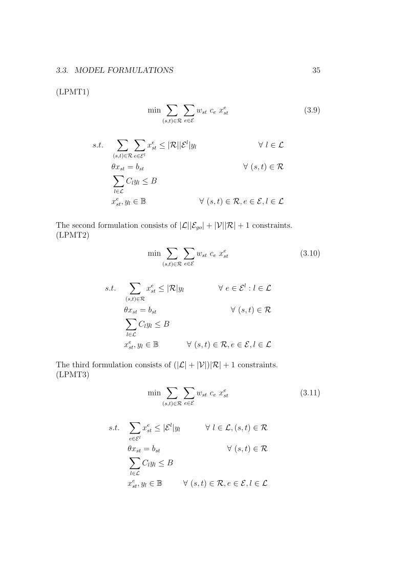
3.3. MODEL FORMULATIONS 35
(LPMT1)
min∑
(s,t)∈R
∑e∈E
wst ce xest (3.9)
s.t.∑
(s,t)∈R
∑e∈El
xest ≤ |R||E l|yl ∀ l ∈ L
θxst = bst ∀ (s, t) ∈ R∑l∈L
Clyl ≤ B
xest, yl ∈ B ∀ (s, t) ∈ R, e ∈ E , l ∈ L
The second formulation consists of |L||Ego| + |V||R| + 1 constraints.(LPMT2)
min∑
(s,t)∈R
∑e∈E
wst ce xest (3.10)
s.t.∑
(s,t)∈R
xest ≤ |R|yl ∀ e ∈ E l : l ∈ L
θxst = bst ∀ (s, t) ∈ R∑l∈L
Clyl ≤ B
xest, yl ∈ B ∀ (s, t) ∈ R, e ∈ E , l ∈ L
The third formulation consists of (|L| + |V|)|R| + 1 constraints.(LPMT3)
min∑
(s,t)∈R
∑e∈E
wst ce xest (3.11)
s.t.∑e∈El
xest ≤ |E l|yl ∀ l ∈ L, (s, t) ∈ R
θxst = bst ∀ (s, t) ∈ R∑l∈L
Clyl ≤ B
xest, yl ∈ B ∀ (s, t) ∈ R, e ∈ E , l ∈ L

36 CHAPTER 3. A NEW MODEL
The fourth formulation consists of (|L||Ego| + |V|)|R| + 1 constraints.(LPMT4)
min∑
(s,t)∈R
∑e∈E
wst ce xest (3.12)
s.t. xest ≤ yl ∀ (s, t) ∈ R, e ∈ E l : l ∈ L
θxst = bst ∀ (s, t) ∈ R∑l∈L
Clyl ≤ B
xest, yl ∈ B ∀ (s, t) ∈ R, e ∈ E , l ∈ L
3.3.3 Bicriteria formulation
As we have mentioned above we have to restrict the number of lines allowedto be chosen out of the line pool. Otherwise all lines of the line pool wouldbe chosen which is not affordable by any company. In Section 3.3.2 we havetreated this problem by introducing the budget constraint (3.4). Of courseit would also be possible to minimize the number of lines while minimizingthe inconvenience of the passengers at the same time. This can be doneby formulating bicriteria programs which can be solved using methods ofmultiobjective optimization.
Basics of bicriteria optimization (e.g. [Ehr00])
The bicriteria optimization problem we consider in this section is given bya discrete set of feasible points X ⊆ Z
n and two objective functions f1, f2 :X → R.
(BP)
minx∈X
(f1(x)f2(x)
)
Definition 3.14. (e.g. [Ehr00]) Let x1, x2 ∈ X
• x1 dominates x2 iff1(x1) ≤ f1(x2)

3.3. MODEL FORMULATIONS 37
and
f2(x1) ≤ f2(x2)
where at least one of the inequalities is strict.
• x ∈ X is a Pareto solution, if there does not exist any y ∈ X thatdominates x.
The goal in bicriteria optimization is to determine the Pareto solutions, i.e.,the set of all x ∈ X which are non-dominated. However, it often is enoughto know the objective values of the Pareto solutions. To this end, let
f(X) =
{(f1(x)f2(x)
): x ∈ X
}
denote the objective space of (BP). Then a point
(f1(x)f2(x)
)∈ f(X) is called
efficient, if x ∈ X is a Pareto solution.
For an illustration, see Figure 3.8. In this example let us assume that the setof objective values for all points x ∈ X is given by the points depicted in thefigure. Then the five filled points p1, . . . , p5 are not dominated by any otherpoint, i.e. exactly these points are efficient.
For finding Pareto solutions we can solve a one-criteria optimization problem.This method is called weighted sum scalarization.
Theorem 3.15. (e.g. [Ehr00]) If x is an optimal solution of
(BP(λ))
minx∈X
λf1(x) + (1 − λ)f2(x)
for some 0 < λ < 1 then x is a Pareto solution of (BP).
Unfortunately, not all Pareto solutions can be found by weighted sum scalar-ization, if the set X ⊆ Z
n consists of a discrete set of points. In Figure3.8, the efficient points p1, p2 and p5 can be found by solving a weightedsum problem, while no λ exists such that p3 and p4 are optimal solutions of(BP(λ)).
Definition 3.16. (e.g. [Ehr00]) A Pareto solution x is called supported ifthere exists a λ with 0 < λ < 1 such that x is the optimal solution of (BP(λ)).

38 CHAPTER 3. A NEW MODEL
��������������������������������
p1
p2p3
p4
p5
f1
f2
Figure 3.8: Efficient solutions of bicriteria optimization problem.
Note that the name supported is due to the following fact: If x is a supported
Pareto solution, then f(x) =
(f1(x)f2(x)
)lies on the boundary of the convex
hull of f(X). Hence there exists a supporting line of f(X) passing throughf(x).
By weighted sum scalarization, we find the set of supported Pareto solutions.With the following result we find also non-supported Pareto solutions. It usesthe constraint version of (BP).
Lemma 3.17. ([HC83]) Let {i, j} = {1, 2} and let x be a unique optimalsolution of
min{fi(x) : x ∈ X and fj(x) ≤ yj}
for some yj. Then x is a Pareto solution of (BP).
Using Lemma 3.17 to find Pareto solutions is known as the ε-constraintmethod, see e.g. [Ehr00].

3.3. MODEL FORMULATIONS 39
Bicriteria line planning problem
We now reformulate our line planning problem as a bicriteria problem, min-imizing both
ftime :=∑
(s,t)∈R
∑e∈E
wst ce xest
and
fcost :=∑l∈L
Cl yl
We will present it for one formulation, corresponding to the single criteriaformulation (LPMT1) in Section 3.3.2. Obviously we can formulate threealternative bicriteria formulations by changing the coupling constraints (3.5)to (3.6), (3.7) or (3.8).
The bicriteria line planning model with minimal transfers:
(BLPMT1)
min
(ftime
fcost
)(3.13)
s.t.∑
(s,t)∈R
∑e∈El
xest ≤ |R||E l|yl ∀ l ∈ L
θxst = bst ∀ (s, t) ∈ R
xest, yl ∈ B ∀ (s, t) ∈ R, e ∈ E , l ∈ L
If we apply the weighted sum scalarization method of theorem 3.15, we getas single objective function
min W1ftime + W2fcost
with 0 < W1 < 1 and W2 = 1 − W1. But this means comparing apples andoranges. The problem to find an appropriate weights W1 and W2 such thatthe obtained solution represents the wishes of the decision maker might bevery difficult.
Applying the ε-constrained method of Lemma 3.17, and setting yj to thebudget B, we get the following one-criteria ε-constraint problem resultingfrom (BLPMT1):

40 CHAPTER 3. A NEW MODEL
(BLPMT-time)
min ftime (3.14)
s.t.∑
(s,t)∈R
∑e∈El
xest ≤ |R||E l|yl ∀ l ∈ L
θxst = bst ∀ (s, t) ∈ R
fcost ≤ ycost
xest, yl ∈ B ∀ (s, t) ∈ R, e ∈ E , l ∈ L
Due to Lemma 3.17 we have the following result.
Lemma 3.18. Let (x, y) be a unique optimal solution of (BLPMT-time).Then (x, y) is a Pareto solution of (BLPMT). If more than one optimalsolution of (BLPMT-time) exists, the solutions that additionally minimizefcost are Pareto solutions.
Unfortunately, (BLPMT-time) is hard to solve.
Corollary 3.19. (BLPMT-time) is NP-hard.
Proof. Setting ycost to the budget B, this model is equal to (LPMT1) whichis already shown to be NP-hard. �
This approach reflects exactly what a decision maker would do intuitively inreal world if we would give him a set of Pareto optimal solutions and leavehim to choose one of them. It is obvious that the more lines one can estab-lish, the better the solution is for the passengers but on the other hand, themore costly it is for the company. So the decision maker would check howmuch money the company is willing to spend and would set an upper boundon the second objective. Note that this is exactly, what we do in our singleobjective formulation (LPMT1).
Since there exist much more powerful solution methods for single objectiveprogramming than for multiobjective programming we will treat only thesingle-objective formulations of (LPMT) in the following. The relaxation ofthe bicriteria programs by using the budget constraint (3.4) is acceptablesince in real world applications a financial budget that must not be exceededis always given.

3.3. MODEL FORMULATIONS 41
3.3.4 Formulation including frequencies
In (LPMT) we implicitly assume that all customers traveling from station sto station t choose the same path in the change&go network, i.e., the sameset of lines. This can be done if edge capacities are neglected in (LPMT). Inpractice, this is usually not the case, since each vehicle only can transport alimited number of customers and usually there is only a limited number ofvehicles possible along each line (e.g. due to safety rules). In the following,we therefore present an extension of (LPMT) taking into account the numberof vehicles on each line in a given time period. Consequently, this formulationallows to split customers along different paths from s to t in the change&go-network GCG.Let N denote the capacity of a vehicle and let the new variables fl ∈ N
contain the frequency of line l, i.e., the number of vehicles running along linel within a given time period. Furthermore we choose variables xe
st ∈ N andchange the vector bst to
bist =
⎧⎨⎩
wst if i = (s, 0)−wst if i = (t, 0)
0 else
Then the Line Planning Model with minimal transfers and frequencies(LPMTF) is the following:
(LPMTF)
min∑
(s,t)∈R
∑e∈E
ce xest (3.15)
s.t.
1
N
∑(s,t)∈R
xest ≤ fl ∀ l ∈ L, e ∈ El (3.16)
θxst = bst ∀ (s, t) ∈ R (3.17)∑l∈L
Clfl ≤ B (3.18)
∑l∈L:k∈El
fl ≤ fmaxk ∀ k ∈ E (3.19)
xest, fl ∈ N ∀ (s, t) ∈ R, e ∈ E , l ∈ L (3.20)

42 CHAPTER 3. A NEW MODEL
Constraints (3.16) make sure that the frequency of a line is high enough totransport the passengers. If fl = 0, line l is not chosen in the line concept.Constraints (3.17) are flow conservation constraints routing the passengersthrough the network. Note that the xe
st variables can take integer values, suchthat passengers may choose different paths for the same origin-destinationpair. Constraint (3.18) is again the budget constraint but with costs for eachvehicle of a line (which are multiplied by the frequency to get the costs ofthe line). The capacity constraint (3.19) may be included if upper boundsfor the frequencies are present.
3.4 Discussion of the formulations
3.4.1 Equivalence and strength
In this section we will show that the four formulations of the (LPMT) pre-sented in section 3.3.2 are equivalent and thus will yield the same set offeasible integer solutions. Therefore we first have to repeat some polyhedraltheory. For more details the reader is referred to [Wol98] and [NW88].
First we make precise what we mean by a formulation.
Definition 3.20. ([NW88]) Given an integer program
min{cx : x ∈ X ⊂ Zn}
where X represents the set of feasible points in Zn. We say that
min{cx : Ax ≤ b, x ∈ Zn}
is a valid IP formulation if X = {x ∈ Zn : Ax ≤ b}.
In general there are many choices of (A, b) and it is usually easy to find some(A, b) that yields one. But an obvious choice may not be a good one whenit comes to solving the problem.
Definition 3.21. ([Wol98]) A subset of Rn described by a finite set of linear
constraints P = {x ∈ Rn : Ax ≤ b} is a polyhedron.
Definition 3.22. ([Wol98]) A polyhedron P ⊆ Rn is a formulation for a set
X ⊆ Zn if and only if X = P ∩ (Zn).
Example 3.23. In Figure 3.9 we show two different formulations for the set:
X = {(2, 2), (2, 3), (3, 2), (3, 3), (3, 4), (4, 2)}

3.4. DISCUSSION OF THE FORMULATIONS 43
P1
1 2 3 4 5
0
1
2
3
4
P2
Figure 3.9: Two alternative formulations for the same integer set proposed in
Example 3.11.
We will now show that the integer formulations of the (LPMT) presented inSection 3.3.2 are valid IP formulations for the same integer set. Thereforewe recall that the integer formulations (3.9), (3.10), (3.11), and (3.12) onlydiffer in the coupling constraints (3.5), (3.6), (3.7), and (3.8).∑
(s,t)∈R
∑e∈El
xest ≤ |R||E l|yl ∀ l ∈ L (3.5)
∑(s,t)∈R
xest ≤ |R|yl ∀ l ∈ L, e ∈ E l (3.6)
∑e∈El
xest ≤ |E l|yl ∀ l ∈ L, (s, t) ∈ R (3.7)
xest ≤ yl ∀ e ∈ cEl : l ∈ L, (s, t) ∈ R (3.8)
withxe
st, yl ∈ {0, 1}
Theorem 3.24. The feasible set of (LPMT4), denoted by X4, is included inthe feasible set of the other formulations: X4 ⊆ X1, X4 ⊆ X2, and X4 ⊆ X3.

44 CHAPTER 3. A NEW MODEL
Proof. If a point (x, y) satisfies the constraints
xest ≤ yl ∀ (s, t) ∈ R, e ∈ E l
for all l ∈ L, then summing up
• over all (s, t) ∈ R and e ∈ E l shows that it also satisfies the constraints∑(s,t)∈R
∑e∈El
xest ≤ |R||E l|yl.
Thus X4 ⊆ X1.
• over all (s, t) ∈ R shows that it also satisfies the constraints∑(s,t)∈R
xest ≤ |R|yl ∀ e ∈ E l
and thus X4 ⊆ X2.
• over all e ∈ E l shows that it also satisfies the constraints∑e∈El
xest ≤ |E l|yl ∀ (s, t) ∈ R
and thus X4 ⊆ X3.
�
Theorem 3.25. (LPMT1), (LPMT2), (LPMT3), and (LPMT4) given inSection 3.3.2 are valid IP formulations of the same integer set X.
Proof. We will show that the integer sets X1, X2, and X3 described by(LPMT1), (LPMT2), and (LPMT3), respectively are equal to the integerset X4 described by (LPMT4). Given a feasible solution (x, y) of
• (LPMT1), if yl = 0 then∑
(s,t)∈R
∑e∈El xe
st = 0 and thus xest = 0 for all
(s, t) ∈ R, e ∈ E l : l ∈ L.
• (LPMT2), if yl = 0 then∑
(s,t)∈R xest = 0 for all e ∈ E l and thus xe
st = 0
for all (s, t) ∈ R, e ∈ E l : l ∈ L.

3.4. DISCUSSION OF THE FORMULATIONS 45
• (LPMT3), if yl = 0 then∑
e∈El xest = 0 for all (s, t) ∈ R and thus
xest = 0 for all (s, t) ∈ R, e ∈ E l : l ∈ L.
So, we see that the coupling constraints of (LPMT4) are satisfied in all casesand together with Theorem 3.24, we get that the formulations are equivalent,i.e. X = X1 = X2 = X3 = X4. �
It is easy to see that there is an infinite number of formulations for eachinteger problem. But there are some formulations that are ”better” thanothers and there exists also always an ”ideal” one, which is in general difficultto find. In the following we will give definitions for ”better” and ”ideal” andwill show, that some of our formulations of the (LPMT) are better thanothers.
Definition 3.26. ([NW88]) Given a set P ⊆ Rn, a point x ∈ R
n is a convexcombination of points of P if there exists a finite set of points {x1, . . . , xt} inP and a λ ∈ R
t+, with
t∑i=1
λi = 1
and
x =t∑
i=1
λixi
.The convex hull of P, denoted conv(P ), is the set of all points, that areconvex combinations of points in P .
Proposition 3.27. ([Wol98]) conv(X) is a polyhedron.
Definition 3.28. ([NW88]) x ∈ Q = {x ∈ Rn : Ax ≤ b} is an extreme point
of Q if there do not exist x1, x2 ∈ Q, x1 �= x2, such that x = 12x1 + 1
2x2.
Proposition 3.29. ([Wol98]) The extreme points of conv(X) all lie in X.
Because of these two results, we can replace the IP : {min cx : x ∈ X} bythe equivalent linear program: {min cx : x ∈ conv(X)}. This ideal reductionto a linear program also holds for unbounded integer and mixed integer setswith rational coefficients. The ideal formulation of Example 3.23 is shown inFigure 3.11. As mentioned above this is in general only a theoretical solu-tion, because in most cases there is such an enormous number of inequalitiesneeded to describe conv(X), and there is no simple characterization for them.But how can we compare different formulations? Most integer programmingalgorithms require a lower bound on the value of the objective function, and

46 CHAPTER 3. A NEW MODEL
the efficiency of the algorithm is very dependent on the strength of the bound(see Chapter 6). A lower bound is determined by solving the LP-relaxation
zLP = {min cx : Ax ≤ b, x ∈ Rn}
since P = {x ∈ Rn : Ax ≤ b} ⊇ X = {x ∈ Z
n : Ax ≤ b}. Now, giventwo formulations of X, defined by (Ai, bi) for i = 0, 1, let P i = {x ∈ R
n :Aix ≤ bi} be their formulations and zi
LP = {min cx : Aix ≤ bi, x ∈ Rn} the
lower bound provided by their LP-relaxations. Note that if P 0 ⊆ P 1, thenz0
LP ≥ z1LP . Hence, we get the better bound from the formulation based on
(A0, b0) and we can say that it is the better or stronger formulation.
Definition 3.30. ([Wol98]) Given a set X ⊆ Rn, and two formulations PA
and PB for X, PA is a stronger formulation than PB if PA ⊂ PB.
Lemma 3.31. ([NW88]) Given two formulations PA and PB for the sameinteger set X with PA stronger than PB, then
minx∈X
cx ≥ minx∈PA
cx ≥ minx∈PB
cx.
Example 3.32. In Figure 3.10, the formulation P3 is better than the for-mulations P1 and P2 which are not comparable, but it is still worse thanthe ideal formulation shown in Figure 3.11.
Notation 3.33. In this section we will denote the feasible set described bythe LP-relaxation of (LPMT1) by P1. We get it by restricting the variablesto 0 ≤ xe
st ≤ 1 for all (s, t) ∈ R, e ∈ E and 0 ≤ yl ≤ 1 for all l ∈ L instead to{0, 1}.The corresponding polyhedra described by (LPMT2), (LPMT3), and (LPMT4)are denoted by P2, P3, and P4, respectively.
Lemma 3.34. Using Notation 3.33, we get P4 ⊆ P1, P4 ⊆ P2, and P4 ⊆ P3.
Proof. If a point (x, y) satisfies the constraints
xest ≤ yl ∀ (s, t) ∈ R, e ∈ E l
for all l ∈ L, we get that
yl ≥ maxe∈El
max(s,t)∈R
xest
for all l ∈ L. Summing up

3.4. DISCUSSION OF THE FORMULATIONS 47
P1
P3
1 2 3 4 5
0
1
2
3
4
P2
Figure 3.10: P3 is a better formulation of the integer set of Example 3.11 than
P1 and P2, but not ideal.
• over all (s, t) ∈ R and e ∈ E l shows that it also satisfies the constraints∑(s,t)∈R
∑e∈El
xest ≤ |R||E l|yl.
Thus P4 ⊆ P1.
• over all (s, t) ∈ R shows that it also satisfies the constraints∑(s,t)∈R
xest ≤ |R|yl ∀ e ∈ E l
and thus P4 ⊆ P2.
• over all e ∈ E l shows that it also satisfies the constraints∑e∈El
xest ≤ |E l|yl ∀ (s, t) ∈ R
and thus P4 ⊆ P3.

48 CHAPTER 3. A NEW MODEL
����
����
����
����
����
����
P3
P1
1 2 3 4 5
0
1
2
3
4
P2
Figure 3.11: P3 is the ideal formulation of the integer set of Example 3.11.
�
We will now discuss the strength of our formulations. We will demon-strate the results on Example 3.11. Figure 3.12 recalls the correspondingchange&go-network and names the driving edges e1, . . . , e4. Let the set oforigin-destination pairs be R = {(1, 2), (1, 3)}. Figure 3.13 and 3.14 showtwo feasible path-combinations for the two customers. We will call themalternative A and alternative B. The corresponding feasible point reads likefollows: if edge ei is depicted in the figure for customer j, then xei
j = 1 andzero otherwise. The yl will be explained in the proofs.
Theorem 3.35. P4 is stronger than P1.
Proof. In Lemma 3.34 we have shown that P4 ⊆ P1.To show that P4 ⊂ P1, we need to find a point in P1 that is not in P4.In our example, the solution (x, y) with the x-values of alternative A (Figure3.13) and y = (1
2, 0, 1
2) is a feasible point in P1 but not in P4 since e.g.
constraint xe1
1 ≤ y1 is violated.More general, a solution in which not all driving edges of a line are used by allorigin-destination pairs, i.e. ∃e∗ ∈ E l∗ such that xe∗
ab = 0 for some (a, b) ∈ R,

3.4. DISCUSSION OF THE FORMULATIONS 49
driving edge
changing edge
in/out edge
1,0
1,l1 2,l1 2,l2 3,l2
1,l3 2,l3 3,l3
3,0
2,0
e1 e2
e4e3
Figure 3.12: The change&go graph of Example 3.11.
and
yl :=
∑(s,t)∈R
∑e∈El xe
st
|R||E l|
for all l ∈ L lies in P1 \ P4. �
Theorem 3.36. P4 is stronger than P2.
Proof. In Lemma 3.34 we have shown that P4 ⊆ P2.To show that P4 ⊂ P2, we need to find a point in P2 that is not in P4.In our example, the solution (x, y) with the x-values of alternative A (Figure3.13) and y = (1
2, 0, 1
2) is a feasible point in P2 but not in P4 since e.g.
constraint xe1
1 ≤ y1 is violated.More general, a solution (x, y) in which one line is not used at all by onecustomer, i.e. ∃(a, b) ∈ R, l∗ ∈ L such that xe
ab = 0 for all e ∈ E l∗ but thereis another edge of this line used by some customer, i.e. ∃(c, d) ∈ R, (c, d) �=(a, b) such that xe
cd = 1 for some e ∈ E l∗ and
yl = maxe∈El
∑(s,t)∈R xe
st
|R|
for all l ∈ L lies in P2 \ P4. �

50 CHAPTER 3. A NEW MODEL
1,0
1,l1 2,l1 2,l2 3,l2
1,l3 2,l3 3,l3
3,0
2,0
e1
e4e3
customer (1,2)
customer (1,3)
Figure 3.13: path combination: alternative A.
Theorem 3.37. P4 is stronger than P3.
Proof. In Lemma 3.34 we have shown that P4 ⊆ P3.To show that P4 ⊂ P3, we need to find a point in P3 that is not in P4.In our example, the solution (x, y) with the x-values of alternative B (Figure3.14) and y = (0, 1, 1
2) is a feasible point in P3 but not in P4 since e.g.
constraint xe3
1 ≤ y3 is violated.More general, a solution (x, y) in which there is one edge of a line that is notused by any customer, i.e. ∃ e∗ ∈ l∗ such that xe∗
st = 0 for all (s, t) ∈ R butthere is another edge of this line used by some customer, i.e. ∃ e ∈ E l∗ , e �= e∗
such that xest = 1 for some (s, t) ∈ R, and
yl = max(s,t)∈R
∑e∈El xe
st
|E l|
for all l ∈ L lies in P3 \ P4. �
Theorem 3.38. P2 is stronger than P1.
Proof. If a point (x, y) satisfies the constraints∑(s,t)∈R
xest ≤ |R|yl ∀ e ∈ E l,

3.4. DISCUSSION OF THE FORMULATIONS 51
1,0
1,l1 2,l1 2,l2 3,l2
1,l3 2,l3 3,l3
3,0
2,0
e2
e3
customer (1,3)
customer (1,2)
Figure 3.14: path combination: alternative B.
then summing up over e ∈ E l shows that it also satisfies the constraints∑(s,t)∈R
∑e∈El
xest ≤ |R||E l|yl
and thus P2 ⊆ P1.To show that P2 ⊂ P1, we need to find a point in P1 that is not in P2.In our example, the solution (x, y) with the x-values of alternative B (Figure3.14) and y = (0, 1
2, 1
2) is a feasible point in P1 but not in P2 since e.g.
constraint∑
(s,t)∈R xe3
st ≤ 2 · y3 is violated.
More general, a solution (x, y) in which there is an edge that is not used byall customers, i.e. ∃e∗ ∈ l∗ such that xe∗
st = 0 for some (s, t) ∈ R but there isan edge of this line that is used by all customers, i.e. ∃e ∈ E l∗ , e �= e∗ suchthat xe
st = 1 for all (s, t) ∈ R, and
yl :=
∑(s,t)∈R
∑e∈El xe
st
|R||E l|
for all l ∈ L lies in P1 \ P2. �
Theorem 3.39. P3 is stronger than P1.

52 CHAPTER 3. A NEW MODEL
Proof. If a point (x, y) satisfies the constraints∑e∈El
xest ≤ |E l|yl ∀ (s, t) ∈ R,
then summing over up (s, t) ∈ R shows that it also satisfies the constraints∑(s,t)∈R
∑e∈El
xest ≤ |R||E l|yl
and thus P3 ⊆ P1.To show that P3 ⊂ P1, we need to find a point in P1 that is not in P3.In our example, the solution (x, y) with the x-values of alternative A (Figure3.13) and y = (1
2, 0, 1
2) is a feasible point in P1 but not in P3 since e.g.
constraint∑
e∈E1 xe1 ≤ 1 · y1 is violated.
More general, a solution (x, y) in which there is an edge that is not used byall customers, i.e. ∃e ∈ E l∗ such that xe
st = 0 for some (s, t) ∈ R but thereis a customer that uses all edges of a line, i.e. ∃(a, b) ∈ R such that xe
ab = 1for all e ∈ E l∗ , and
yl =
∑(s,t)∈R
∑e∈El xe
st
|R||E l|
for all l ∈ L lies in P1 \ P3. �
Theorem 3.40. Comparing P2 and P3, none of them is stronger than theother.
Proof. We can find a point, that is in P2 but not in P3 and vice versa.In our example, the solution (x, y) with the x-values of alternative B (Figure3.14) and y = (0, 1
2, 1) is a feasible point in P2 but not in P3 since e.g.
constraint∑
e∈E2 xe3 ≤ 1 · y2 is violated.
More general, a solution (x, y) in which there is a customer that uses all edgesof a line, i.e. ∃(a, b) ∈ R such that xe
ab = 1 for all e ∈ l∗ but there is no edgeof this line that is used by all customers, i.e. xe
st = 0 for some (s, t) ∈ R forall e ∈ E l∗ , and ∑
(s,t)∈R
xest = k < |R|
and
yl = maxe∈El
∑(s,t)∈R xe
st
|R|
for all l ∈ L lies in P2 \ P3.

3.4. DISCUSSION OF THE FORMULATIONS 53
On the other hand, in our example, the solution (x, y) with the x-values ofalternative B (Figure 3.14) and y = (0, 1, 1
2) is a feasible point in P3 but not
in P2 since e.g. constraint∑
(s,t)∈R xe3
st ≤ 2 · y3 is violated.
More general, a solution (x, y) in which there is an edge that is used by allcustomers, i.e. ∃e∗ ∈ E l∗ such that xe∗
st = 1 for all (s, t) ∈ R but there is acustomer that does not use all edges of this line, i.e. ∃(a, b) ∈ R such thatxe
ab = 0 for some e ∈ E l∗ , e �= e∗, and
yl := max(s,t)∈R
∑e∈El xe
st
|E l|
for all l ∈ L lies in P3 \ P2. �
Remark 3.41. Note that in real world instances (LPMT3) comes out to bemuch better than (LPMT2) (see Table 3.5). Unfortunately, due to its hugeamount of constraints it is only computable for smaller instances (see Table3.4).
Figure 3.15 shows schematically the results of this section. All formulationsdescribe the same integer set but the (LPMT4) formulation is better than allothers. (LPMT1) is the worst and (LPMT2) and (LPMT3) are not compa-rable but better than (LPMT1) and worse than (LPMT4). Later we will seethat in real world instances (LPMT3) figures out to be better than (LPMT2)in most cases (see Section 3.4.3).
P4
P3
P2
P1
Figure 3.15: Schematical summary of the results of Section 3.4.

54 CHAPTER 3. A NEW MODEL
3.4.2 Model structure
Integer programs and their associated linear relaxations encountered in appli-cations almost always exhibit a large deal of structure. Constraint matricesare typically very sparse, having non zero elements in the order of magnitudeof one percent, or less. This well known phenomenon is due to the fact thatactivities associated with variables are subject to only a few of the condi-tions represented by the constraints, respectively. On top of that, there mayexist a hierarchical, geographical or logical segmentation of the underlyingproblem, which is reflected in the model formulation. Thus, it is likely thatthe non zeros are grouped in such a way that independent subsystems of vari-ables and constraints result, possibly linked by a distinct set of constraintsand/or variables. Figure 3.16 shows schematically the distribution of non ze-ros for different angular block diagonal matrices, occurring in practice mostfrequently ([Min86]).
Figure 3.16: Block diagonal matrix structure, (a) with coupling constraints, (b)
with coupling variables, and (c) with coupling constraints and variables. Only the
shaded regions may contain non-zero elements.
All our model formulations presented in Section 3.3.2 have block diagonalstructure with only a few coupling constraints and all blocks (except thesingle budget constraint) are totally unimodular.
The block structure of the model (LPMT1) is shown in the following scheme.
min∑
(s,t)∈R
∑e∈E wstcex
est
∑(s,t)∈R
∑e∈El xe
st ≤ |R||E l|yl coupling constraints (3.5)
θxs1t1 = bs1t1
. . . (3.3)
θxs|R|,t|R|= bs|R|,t|R| ∑
l∈L Clyl ≤ B (3.4)

3.4. DISCUSSION OF THE FORMULATIONS 55
Note that the other formulations (LPMT2), (LPMT3), and (LPMT4) onlydiffer in the coupling constraints (3.6), (3.7), and (3.8) and thus the structureis equivalent.The shortest path constraint set (3.3) decomposes in |R| many independentblocks: one for each origin-destination pair (s, t) ∈ R. These shortest-path-blocks are identical on the left-hand side and differ only in the right-handside bst. We get one more independent block for the budget constraint (3.4).The constraints (3.5) are coupling constraints.
Since the change&go-network and hence the corresponding problem formu-lations get huge, it is not possible to compute the optimal solution of theLP-relaxation of the different formulations using standard optimization soft-ware. Table 3.4 shows the CPU times for some real world instances explainedin Table 3.2 for the different formulations. The results are based on a 3.06GHz Intel4 processor with 2 GB RAM using Xpress IVE Version 1.15.01.The size of (LPMT) depends on two criteria: the size of the line pool andthe number of origin-destination pairs. Table 3.3 shows computation timesof the (LPMT1) relaxation for different line pool sizes and origin-destinationsets.Even though the LP-relaxation of (LPMT) is not solvable for real worldinstances, we can exploit its nice structure to decompose the problem intomany small (solvable) subproblems linked by only few coupling constraints.In Section 5.2 we will present a solution approach based on Dantzig-Wolfedecomposition to solve the LP-relaxation of our problem. Note that in thiscase the subproblems can also be computed on parallel machines since theyare independent.
The size of (LPMT) depends on two criteria:
1. the size of the line pool: the change&go-network is constructed outof the line pool and thus the size of the node-arc incidence matrix θincreases with with the line pool size
2. the number of origin-destination pairs: we solve a shortest path prob-lem for each origin-destination pair and so the number of constraintsincreases if we treat more origin-destination pairs
Table 3.3 shows the CPU times for the LP-relaxation of (LPMT1) for in-stances with different sizes of line pools |L| and sets of origin-destinationpairs |R|. If the problem was not solvable due to lack of memory, this isindicated by ”M”.

56 CHAPTER 3. A NEW MODEL
|L| |R|=2 |R|=10 |R|=50 |R|=100 |R|=150 |R|=200 |R|=147610 0.187 0.860 4.219 8.563 12.469 16.453 154.28150 4.875 23.610 118.844 239.782 361.063 M M100 25.172 124.359 626.640 M M M M132 52.047 257.906 M M M M M150 M M M M M M M
Table 3.3: CPU times for the LP-relaxation of (LPMT1) for different line pool
sizes and origin-destination sets. ”‘M”’ denotes out of memory.
Instance |L| Budget (LPMT1) (LPMT2) (LPMT3) (LPMT4)
0 3 1 0.03 0.03 0.03 0.031 10 7 154.8 146.2 153.3 M2 50 30 M M M M
Table 3.4: CPU times for the LP-relaxation of the four formulations using
XpressMP, ”M” denotes out of memory)
In the next section we will present a method to check if the trivial solution,i.e. the solution we get, if we compute the shortest path problem on thechange&go-network constructed of all lines of the line pool, is already an op-timal solution of the LP-relaxation. Depending on the formulation (LPMT1),(LPMT2), (LPMT3), and (LPMT4), this may appear quite often.
3.4.3 Special cases
In some special cases the solution of the LP-relaxation of the (LPMT1) iseasy to find.
Proposition 3.42. If Cl = 1 ∀ l ∈ L and if for each origin-destination pair(s, t) ∈ R there is a line l ∈ L that serves (s, t) directly on shortest path, thenthe solution that chooses exactly this special line for each origin-destinationpair is always feasible and optimal for the LP-relaxation of (LPMT1).
Proof. Let xest be the optimal solution of the shortest path problem on the
change&go-network constructed of all lines of the line pool and
yl :=
∑(s,t)∈R kl
st
|R||E l|
for all l ∈ L with klst :=
∑e∈El xe
st. Note that klst ≤ |E l| for all (s, t) ∈ R, l ∈
L. Since by assumption each passenger can travel directly on one line, the

3.4. DISCUSSION OF THE FORMULATIONS 57
number of non-zero klst is equal |R|.
This solution (x, y) satisfies the coupling constraints of (LPMT1) (3.5).It also satisfies the budget constraint (3.4)
∑l∈L
Clyl =1
|R|
∑l∈L
∑(s,t)∈R
≤1︷︸︸︷kl
st
|E l|︸ ︷︷ ︸≤|R|
≤ 1
independently of the choice of the budget since a budget smaller than onedoes not make sense if Cl = 1 for all l ∈ L. So, the solution (x, y) is feasiblefor (LPMT1). It is also optimal since there is no better way than travelingon shortest path without transfer. �
Definition 3.43. A trivial solution (x, y1), (x, y2), (x, y3), (x, y4) of (LPMT1),(LPMT2), (LPMT3), (LPMT4), respectively, is defined as the solution of theshortest path problem on the change&go-network constructed of all lines ofthe line pool xe
st and
y1l :=
∑(s,t)∈R
∑e∈El xe
st
|E l||R|∀ l ∈ L (for (LPMT1))
y2l :=
maxe∈El
∑(s,t)∈R xe
st
|R|∀ l ∈ L (for (LPMT2))
y3l :=
max(s,t)∈R
∑e∈El xe
st
|E l|∀ l ∈ L (for (LPMT3))
y4l := max
(s,t)∈Rmaxe∈El
xest ∀ l ∈ L (for (LPMT4))
It is in general not unique and need not to be feasible in the sense that itfulfills the budget constraint.
In real world instances it appears quite often that a trivial solution is anoptimal solution of the LP-relaxation of (LPMT1) even if not all assumptionsof Proposition 3.42 are fulfilled. This is clear since the right hand sides |R||E l|of the coupling constraints (3.5) are chosen such that all passengers could useall edges of all lines. In real world only few edges of the network are usedand so Kl :=
∑(s,t)∈R
∑e∈El xe
st is much smaller than |R||E l|, hence
∑l∈L
Cly1l =
∑l∈L
Cl
Kl
|E l||R|≤ B
is often satisfied.

58 CHAPTER 3. A NEW MODEL
No. |L| obj.val. T1 T2 T3 T4 CPU
1 10 2271.3 0.69 0.99 9.53 10 02 50 9459.9 0.20 0.35 25.31 48 103 100 24780.0 0.13 0.29 41.83 96 604 132 31654.2 0.11 0.26 53.12 129 1315 200 15128.9 0.07 0.19 54.89 197 3426 250 19096.0 0.05 0.16 61.07 235 4187 275 20118.2 0.04 0.15 63.47 252 5798 300 26598.3 0.06 0.19 72.35 282 8119 330 26817.7 0.04 0.16 74.44 302 1052
10 350 26450.0 0.07 0.23 90.04 331 96611 375 27517.8 0.06 0.20 90.75 345 121512 400 34781.3 0.06 0.20 100.05 370 157113 423 35135.5 0.06 0.20 102.19 389 1972
Table 3.5: Minimal budgets such that trivial solution is optimal solution of the
LP-relaxation of the different formulations of the (LPMT), see Lemma 3.44. CPU
times in seconds.
Lemma 3.44. Let i ∈ {1, 2, 3, 4} and let (x, yi) be a trivial solution of(LPMTi), as defined in Definition 3.43. If
Ti :=∑l∈L
Clyil ≤ B
is satisfied, the trivial solution (x, yi) is an optimal solution of the (LPMTi).Note that for i = 4 the solution (x, y4) of the LP-relaxation of (LPMT4) isinteger and thus if T4 ≤ B holds, the trivial solution is an optimal solutionto the original problem.
Proof. Clear by the formulation of (LMPT1), (LMPT2),(LPMT3), and(LMPT4). �
Table 3.5 shows some computational results of real world instances of Lemma3.44 with line costs Cl = 1 ∀ l ∈ L. T1, T2, T3 and T4 represent the minimalbudgets such that the trivial solution still is the optimal solution of the LP-relaxation of the corresponding formulation. This means, if the given budgetis smaller than the Ti-value, the trivial solution does not fulfill the budgetconstraint and we have to use other methods to find a solution of the LP-relaxation. Our approach is a Dantzig-Wolfe decomposition approach andwill be presented in Chapter 5.
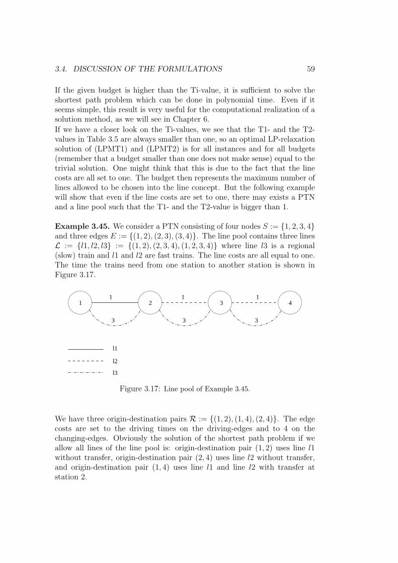
3.4. DISCUSSION OF THE FORMULATIONS 59
If the given budget is higher than the Ti-value, it is sufficient to solve theshortest path problem which can be done in polynomial time. Even if itseems simple, this result is very useful for the computational realization of asolution method, as we will see in Chapter 6.
If we have a closer look on the Ti-values, we see that the T1- and the T2-values in Table 3.5 are always smaller than one, so an optimal LP-relaxationsolution of (LPMT1) and (LPMT2) is for all instances and for all budgets(remember that a budget smaller than one does not make sense) equal to thetrivial solution. One might think that this is due to the fact that the linecosts are all set to one. The budget then represents the maximum number oflines allowed to be chosen into the line concept. But the following examplewill show that even if the line costs are set to one, there may exists a PTNand a line pool such that the T1- and the T2-value is bigger than 1.
Example 3.45. We consider a PTN consisting of four nodes S := {1, 2, 3, 4}and three edges E := {(1, 2), (2, 3), (3, 4)}. The line pool contains three linesL := {l1, l2, l3} := {(1, 2), (2, 3, 4), (1, 2, 3, 4)} where line l3 is a regional(slow) train and l1 and l2 are fast trains. The line costs are all equal to one.The time the trains need from one station to another station is shown inFigure 3.17.
l1
l2
l3
3 3 3
1111 2 3 4
Figure 3.17: Line pool of Example 3.45.
We have three origin-destination pairs R := {(1, 2), (1, 4), (2, 4)}. The edgecosts are set to the driving times on the driving-edges and to 4 on thechanging-edges. Obviously the solution of the shortest path problem if weallow all lines of the line pool is: origin-destination pair (1, 2) uses line l1without transfer, origin-destination pair (2, 4) uses line l2 without transfer,and origin-destination pair (1, 4) uses line l1 and line l2 with transfer atstation 2.

60 CHAPTER 3. A NEW MODEL
In this case, we get the following Ti-values as defined in Lemma 3.44:
T1 =2
3+
4
6+
0
9=
4
3
T2 =2
3+
2
3+
0
3=
4
3
T3 =1
1+
2
2+
0
3= 2
T4 = 1 + 1 + 0 = 2
Thus, choosing line l1 and line l2 would be the optimal solution if the budgetis set to 2 or 3. If it is set to 1, the optimal solution is the line conceptL = {l3} because it is the only line that serves all customers.
The T3-values are much ”better” than the T1- and the T2-values in thesense that the solution of the LP-relaxation of (LPMT3) is not equal to thetrivial solution if the given budget is smaller than the relatively high T3-value, and hence is stronger. So, in practice we can say, that the (LPMT3)formulation is stronger than the (LPMT2) formulation even if we have shownin Theorem 3.40 that they are not comparable. But this means only thatthere exists a case in which one formulation is stronger than the other andvice versa. This case is mentioned in the proof of the theorem. It uses thefact that y2
l is near one if there is an edge of a line l that is used by almost allcustomers which hardly ever appears in real world instances. On the otherhand y3
l is near one if almost all edges of a line l are used by some customer,which is much more likely since there may be a customer that uses a linefrom the start- to the end-node and by doing so, he reaches his destinationwithout transfer. Unfortunately the (LPMT3) formulation also has muchmore constraints than (LPMT2) and so the solution of the LP-relaxation iscomputationally hard for larger instances (see Table 3.4).As we have shown in Section 3.4 the (LPMT4) formulation yields the bestTi-values of all formulations. Calculating its LP-relaxation would rise upto a highly integer solution but unfortunately it has too many constraintsto solve even small instances with standard LP solvers. Even the resultingmaster problem in the Dantzig-Wolfe approach presented in Chapter 5 getstoo big, so it can only be used for heuristic approaches.

Part II
Solution Methods
61


Chapter 4
Heuristics
As we have seen in Section 3.2 our problem belongs to the class of NP-hardproblems. That is, there is strong evidence that no efficient algorithms for itssolution exist. Fortunately our integer formulations of (LPMT) have a nicestructure. All computational results presented in this section are computedon a Pentium 4 processor with 3Ghz and 2GB RAM. The heuristics are im-plemented using Visual C++ 6.0. Shortest path subproblems are calculatedusing the Dijkstra algorithm.
Notation 4.1. In this section we denote the edge set of a change&go-networkconstructed by the lines of a given line concept L ⊆ L by
E(L) := ∪l∈LEl ∪ Echange ∪ EOD.
Furthermore, to simplify the notation, we will call the origin-destination pairsr ∈ R instead of (s, t) ∈ R.
4.1 Variable Fixing
As we mentioned in Section 3.3.2, the (LPMT4) formulation (3.12) is thestrongest among our formulations and so we will use it as a basis of variousheuristics presented in this chapter.
Therefore we first recall (LPMT4). We remember that the formulation con-sists of the objective function (3.2), the coupling constraints (3.8), the short-est path problems (3.3) and the budget constraint (3.4).
63

64 CHAPTER 4. HEURISTICS
(LPMT4)
min∑r∈R
∑e∈E
wr ce xer (3.2)
s.t. xer ≤ yl ∀ r ∈ R, e ∈ E l : l ∈ L (3.8)∑
e∈E
θiexer = bi
r ∀ r ∈ R, i ∈ V (3.3)
∑l∈L
Clyl ≤ B (3.4)
xer, yl ∈ B ∀ r ∈ R, e ∈ E , l ∈ L
We can divide the variables of the model into two groups: the x-variables andthe y-variables. The x-variables correspond to the choice of the passengerpaths and the y-variables correspond to lines chosen to be in the line concept.
What happens if we fix one of the variable groups?
1. Fixing the y-variables:This means, that we assume the line concept L to be known. Thebudget-constraint thus reduces to
∑l∈L
Cl ≤ B
which does not contain any variables and only makes sure that the cho-sen line concept does not exceed the given budget and thus is feasible.The coupling constraints fix the xe
r to zero for all e ∈ Ego \ E(L) andthus the shortest path constraints reduce to
∑e∈E(L)
θiexer = bi
r ∀ r ∈ R, i ∈ V
The remaining problem we have to solve is

4.2. GREEDY HEURISTICS 65
(LPMT(L))
min∑r∈R
∑e∈E(L)
wr ce xer (4.1)
s.t.∑
e∈E(L)
θiexer = bi
r ∀ r ∈ R, i ∈ V
∑l∈L
Cl ≤ B
xer ∈ B ∀ r ∈ R, e ∈ E
This problem is a shortest path problem and can be solved in polyno-mial time. We denote an optimal solution of (LPMT(L)) by x(L).
2. Fixing the x-variables:This means, we have the paths of the customers already given. Sinceeach driving edge corresponds to exactly one line, we get the solutionof the y-variables straightforwardly by setting
yl := maxr∈R,e∈El
xer ∈ {0, 1}
for all l ∈ L. Again we have to check the budget constraint to find outif the corresponding solution is feasible.
4.2 Greedy heuristics
The idea of a Greedy heuristic is to construct a solution, choosing at eachstep the item bringing the ”best” immediate reward. Often, the solutionsare constructed from scratch starting with the empty set.
4.2.1 Starting with empty set
More formally, we suppose that the problem can be written as a combinatorialproblem in the form. Let c(Q) be a real-valued function defined on all subsetsof X, we consider the problem
min{c(Q) : Q ⊆ X}
.The pure Greedy heuristic can formally be formulated as followed.

66 CHAPTER 4. HEURISTICS
Algorithm 4.2. ([Wol98], [NW88]) Greedy heuristic - general form
1. Set Q0 = ∅ (start with the empty set). Set t = 1.
2. Set jt = arg minj∈X\Qt−1(c(Qt−1 ∪ {j}) − c(Qt−1)) (choose the elementwhose additional cost is minimum).
3. If the previous solution Qt−1 is feasible, and the objective value has notdecreased, i.e. c(Qt−1) ≤ c(Qt−1 ∪ {jt}), stop with QG = Qt−1.
4. Otherwise set Qt = Qt−1 ∪ {jt}.
5. If Qt = X, and solution Qt is feasible, stop with QG = Qt.If Qt is not feasible, stop: problem is infeasible.
6. Otherwise set t := t + 1, and return to 2.
In our case we get a combinatorial problem if we minimize over all possibleline concepts. The corresponding reformulation is:
(CLPMT)
minL⊆L
∑r∈R
∑e∈E(L)
wr ce xer (4.2)
s.t.∑
e∈E(L)
θiexer = bi
r ∀ r ∈ R, i ∈ V (4.3)
∑l∈L
Cl ≤ B (4.4)
xer ∈ B ∀ r ∈ R, e ∈ E(L) (4.5)
Corresponding to the notation of Algorithm 4.3, we define L := Q (lineconcept), Lt := Qt (line concept in tth iteration),
c(L) =∑r∈R
∑e∈E(L)
wr ce xer(L) := c(Q),
where x(L) is a solution of the shortest path problem in the change&go-network constructed from the corresponding line concept L, i.e. a solutionof (LPMT(L)).

4.2. GREEDY HEURISTICS 67
A line concept L is feasible if it satisfies the constraints∑l∈L
Cl ≤ B, (4.6)
and ∑e∈E(L)
θiexer(L) = bi
r ∀ r ∈ R, i ∈ V. (4.7)
We now get the following Greedy algorithm for (LPMT).
Algorithm 4.3. Greedy for (LPMT)
1. Set L0 = ∅ (start with the empty set). Set t = 1.
2. Set
lt = arg minl∈L\Lt−1
(c(Lt−1 ∪ {l}) − c(Lt−1)))
= arg minl∈L\Lt−1
(∑
e∈E(Lt−1∪{l})
∑r∈R
wrcexer(L
t−1∪{l})−∑
e∈E(Lt−1)
∑r∈R
wrcexer(L
t−1))
(choose the line that serves passengers that have not been served yetand shortens the path of passengers that have been served already byanother line).
3. If the previous line concept Lt−1 is feasible, and the objective value hasnot decreased, i.e. c(Lt−1) ≤ c(Lt−1 ∪ {lt}), stop with LG = Lt−1.
4. Otherwise set Lt = Lt−1 ∪ {lt}.
5. If t = |L|, and line concept Lt is feasible, stop with LG = Lt.If Lt is not feasible, stop: problem is infeasible.
6. Otherwise set t := t + 1, and return to 2.
Unfortunately the calculation of the ”best” line in Step 2 is too time con-suming for real world instances. So, we have to find different functions tofind a ”good” line.

68 CHAPTER 4. HEURISTICS
Different line choice criteria in Step 2
The main changes between different Greedy heuristics occur in Step 2 wherewe have to find a criterion that tells us which line to choose for the lineconcept. It should be the one bringing the ”best” immediate reward, as wementioned above. As we are not allowed to exceed a given financial budget,we should choose a line with low line cost Cl. Thus the line costs will be inthe nominator in Step 2. On the other hand, we have to find a line conceptthat serves all passengers. One possibility is to choose the line that coversthe most not yet covered stations in the PTN. The criterion in Step 2 canthus be formulated as:
lt = arg minl∈L\Lt−1
Cl
|S(l) \ ∪t−1i=1S(li)|
with S(l) be the set of all stations of line l.We call the resulting Greedy algorithm Cover Greedy since we try to coverall stations of the PTN first to find a feasible solution as fast as possible.Table 4.1 shows the results and CPU times for different real world instancesexplained on Table 3.2. The line costs are set equal to one for all lines.
No. |L| budget obj.val. CPU
1 10 7 2560.7 02 50 30 10837.6 893 100 50 27550.1 2214 132 70 32059.3 7405 200 70 16298.9 12458 300 70 30521.0 11921
Table 4.1: Solutions of the cover greedy algorithms for different line pool sizes
The next heuristic is based on the following idea: We calculate a trivialsolution (x, y3) of (LPMT3), as defined in Definition 3.43. A line l with ahigh y3
l -value is a line, that is used by some customer on a large numberof edges respectively to the total number of its edges. This means, thereis strong evidence that this client travels directly on shortest path from itsorigin to its destination and so, if on the other hand the line cost of this lineCl is low, it may be a good choice for the line concept.The criterion in Step 2 can thus be formulated as:
lt = arg minl∈L\Lt−1
Cl
y3l

4.2. GREEDY HEURISTICS 69
Note, that the ”importance” (Cl/y3l ) of a line does not depend on the current
line concept Lt−1. So, it is possible to sort the lines by their importance(li1 , . . . , li|L|
) before starting the algorithm. During the algorithm the linesare added successively according their precalculated importance to the lineconcept until a stopping criterion is fulfilled.We call the resulting Greedy algorithm List Greedy since we add the linesaccording to a precalculated list. Table 4.2 shows the results and CPU timesfor different real world instances explained in Table 3.2. The line costs areequal to one for all lines.
No. |L| budget obj.val. CPU
1 10 6 infeasible 01 10 9 2290.3 02 50 30 infeasible 122 50 47 9460.9 1173 100 50 infeasible 163 100 91 24945.1 1304 132 70 infeasible 1344 132 121 32059.3 2925 200 70 infeasible 166
Table 4.2: Solutions of the list greedy algorithms for different line pool sizes
Other line-choice criteria are possible, such as
• Choose the y1-value or the y2-value instead the y3-value in the ListGreedy algorithm.
• Let ODl denote the number of origin-destination pairs that use one ormore driving edges of line l on their shortest path in the change&go-network constructed on the whole line concept:
ODl :=∑r∈R
(maxe∈El
xer) (4.8)
Sort the lines by the minimal cost and maximum ODl value: Cl
ODland
apply this list to the List Greedy algorithm.
Note that in the first iterations of these heuristics the shortest path feasibilitycriterion (4.7) will likely not be fulfilled since there are not enough lines toserve all passengers. To save computation time it is possible to check feasi-bility in these first iterations by checking shortest path in the corresponding(smaller) line-change-graph presented in Section 3.3.1 (see Figure 3.7).

70 CHAPTER 4. HEURISTICS
4.2.2 Starting with line pool
So far we started with an empty line concept and added lines successively.In this subsection we present heuristics that work the opposite way around.We start with the complete line pool as line concept and delete successivelyexpensive, unimportant lines until the budget constraint is fulfilled and noimprovement of the objective value is possible. We call this kind of heuristicdelete heuristics.Note that this is a way to implement the Relaxation-and-Separation Heuris-tic explained in Section 4.3, since we successively set some ylt = 0 and byadjusting the corresponding change&go-network, we set the correspondingxe
st = 0 for all e ∈ E lt .
Algorithm 4.4. Delete heuristic - general form
1. Set L0 = L (start with line pool as line concept). Set t = 1.
2. Set lt = arg maxl∈L\LtCl
W (l)(choose the line with maximal cost and
minimal relevance, measured by some relevance function W ).
3. If the previous solution Lt−1 is feasible, and the objective function valuehas not decreased, stop with LD = Lt−1.
4. Otherwise set Lt = Lt−1 \ {jt}.
5. Otherwise set t := t + 1, and return to 2.
As before, feasibility has to be checked concerning
• the budget constraint (4.6)
• the shortest path constraints (4.7)
But now, in the beginning of the algorithm, the budget constraint is violatedand the shortest path constraints are satisfied. Therefore we have to check ineach iteration the length of the shortest paths in the real change&go-graphand not as in the first iterations of the Greedy heuristics that start with anempty set, in the shrunken line-change-graph and thus the computationaleffort increases.
We have various possibilities to choose the relevance function in Step 2 ofthe algorithm.

4.3. RELAXATION AND SEPARATION 71
1. Let ODl(L) denote the number of origin-destination pairs that use oneor more driving edges of line l on their shortest path in the change&go-network constructed by the current line concept L:
ODl(L) :=∑r∈R
(maxe∈El
xer(L)) (4.9)
Then, the relevance function can be set to:
W (l) := ODl
We call this algorithm OD-delete heuristic. Table 4.3 shows solutionvalues and CPU times for different instance sizes.
2. Let xest(L) denote the solution of the shortest path problem of origin-
destination pair (s, t) ∈ R in the change&go-network constructed bythe current line concept L. Then
W (l) :=∑e∈Elt
∑(s,t)∈R
xest(L)
We call this algorithm path-delete heuristic. Table 4.4 shows solutionvalues and CPU times for different instance sizes.
Of course many other relevance functions are possible such as sorting thelines in advance by their yi-value of Lemma 3.44 for i = 1, 2, or 3 and settingthe relevance function to
W (l) := yi.
4.3 Relaxation and Separation
In this section we relax the given problem (LPMT4) by ignoring the couplingconstraints
xest ≤ yl ∀ (s, t) ∈ R, e ∈ E l : l ∈ L
to get a polynomial solvable problem, namely a shortest path problem withsolution vector x. In a second step, the separation step, we calculate thevalues of the y-variables as mentioned in Section 4.1 (Fixing the x-variables)and consider the coupling constraints that are not satisfied by the shortestpath solution. In this case there is a xe
st with
xest > yl.
Now we have two possibilities. We can set xest := 0 or yl := 1.

72 CHAPTER 4. HEURISTICS
No. |L| budget obj.val. CPU
1 10 6 2615.2 32 50 30 9828.1 1613 100 50 27695.3 21314 132 70 31854.5 44055 200 70 15721.2 303935 200 180 15133.4 44416 250 200 19116.3 246757 300 250 26624.8 461858 330 50 28510.2 348654
Table 4.3: Delete OD-heuristics for different line pool sizes
No. |L| budget obj.val. CPU
1 10 6 2615.2 22 50 30 9926.9 1612 50 40 9525.4 853 100 50 26008.4 30363 100 80 14912.2 12554 132 70 32504.0 89544 132 100 31843.2 48065 200 70 15689.2 297645 200 180 15131.3 41696 250 200 19114.5 162067 300 250 26616.5 357508 330 50 28415.6 331672
Table 4.4: Delete path-heuristics for different line pool sizes

4.4. LINE SEGMENT HEURISTIC 73
1. If we set xest := 0, this means that we do not allow any passenger to
use this driving edge. We delete the edge from the change&go-graph,but we do not change the problem itself. The remaining problem stillis a shortest path problem.
2. It we set yl := 1, this means that this line has to be in the line conceptand we can delete its cost Cl from the budget.
More formally we get the following algorithm:
Algorithm 4.5. Relaxation and separation - general form
1. Solve (LPMT4) without the coupling constraints 3.8 with solution xand compute the corresponding y-values.
2. Feasibility check: If xest ≤ yl is true for all (s, t) ∈ R, e ∈ E l : l ∈ L
then stop with L := {l ∈ L : yl = 1}Otherwise: there is at least one xe
st > yl, e ∈ E l
3. Add the constraint xest = 0 to the relaxed (LPMT4) and goto Step 1.
This idea will be discussed in more detail in Section 6.
4.4 Line segment heuristic
In the heuristics introduced so far, the lines have always been chosen from agiven line pool. The heuristic we will present in this section will construct thelines from scratch. Nevertheless it uses the idea of the change& go-network.
Notation 4.6. We denote by Vs := {(s, l) ∈ V} the set of all nodes in thechange& go-graph that correspond to node s ∈ S of the underlying PTNand by Es := {{(s, l1), (s, l2)} ∈ Echange} all changing edges of the change&go-graph between lines that stop at station s ∈ S of the PTN.
Idea: The line pool is initially constructed by defining each edge in the PTN tobe a line. We construct the corresponding change&go-network and calculateshortest paths for all origin-destination pairs to get the solution xe
st. So, weget values ve for all changing edges e ∈ Echange:
ve :=∑
(s,t)∈R
xest ∀ e ∈ Echange.
Now, for each station in the PTN, we consider all corresponding changingedges Es and solve the weighted matching problem for them, which is solvablein polynomial time.

74 CHAPTER 4. HEURISTICS
Definition 4.7. ([Wol98]) Given a graph G = (V,E). A matching M ⊆ Eis a set of disjoint edges, that is, at most one edge of a matching is incidentto any node v ∈ V .
Definition 4.8. ([NW88]) Given a graph G = (V,E) with m nodes and nedges, and integral weights ce for e ∈ E. The weighted matching problem canbe given in the integer programming formulation as follows:
max∑e∈E
cexe
s.t.∑
e∈δ(i)
xe ≤ 1 ∀ i ∈ V
x ∈ Zn+
where δ(i) is the set of edges incident to node i. This means, we want to findthe matching with the maximum sum of the edge-costs of the edges containedin the matching.
If an edge e = {(s, l1), (s, l2)} is in the matching M we join the lines l1 andl2 to a new (longer) line l∗. Doing so for each station of the PTN we end upwith a line concept that serves all passengers. As we join the line segmentswhere initially many people had to change to a new line we assure that thesepeople have no transfer at this station and so the number of transfers in thenetwork stays small.
Example 4.9. In Figure 4.1 we see a part of a change& go-network. In thebig circle we see all nodes and edges corresponding to station s ∈ S of theunderlying PTN. The numbers on the changing edges correspond to the edgecosts. They represent the number of passengers that would have to changebetween the corresponding lines. The thick lines represent the solution ofthe weighted matching. We now join the lines l2 = (b, s) and l5 = (s, e) to anew line l∗ := (b, s, e) and the lines l3 = (c, s) and l4 = (s, d) to a new linel′ := (c, s, d). Line l1 = (a, s) ends at station s.
4.5 Summary
The heuristics starting with the empty set (in the following named add-heuristics are much faster than the heuristics starting with the complete linepool (called delete-heuristics). This has many reasons:

4.5. SUMMARY 75
s,l1
s,l2
s,l3
s,l4s,l5
1
2
4
6
1
7 2
5
5
2
Station s
a,l1
b,l2
c,l3
d,l4e,l5
changing edges
matching
driving edges
Figure 4.1: Joining lines in the line segment heuristic.
• In real-world instances the budget is much smaller than the numberof possible lines in the line pool. Thus, a heuristic that starts withan empty set and adds in each iteration one line needs less iterationsthan a heuristic that deletes a line from the complete line pool in eachiteration.
• The solutions of the add-heuristics are in the first iterations infeasiblewith respect to the shortest path constraints. Thus, as we mentionedabove, it is sufficient to check feasibility using the much smaller line-change-graph. This is not possible for the delete-heuristics since theirsolutions satisfy the shortest path constraints in the beginning, butviolate the budget constraint.
• Solving the shortest path problems of the current change&go-networkis the most time consuming step and has to be done in each iterationin the delete-heuristics in contrary to the add-heuristics, where once,the current line concept is feasible and the shortest paths for all origin-destination pairs are computed, we only have to update the paths thatmay change by adding the new line. This can be done much fasterthan solving the shortest path problem of the updated network for allorigin-destination pairs in each step.

76 CHAPTER 4. HEURISTICS
Figure 4.2 shows graphically the CPU times of the three main heuristics fordifferent line pool sizes.On the other hand, the delete-heuristics are more reliable in finding a feasiblesolution. As we have seen in Table 4.2, the list-heuristic, which is one of theadd-heuristics hardly ever finds a feasible solution. This happens if the sumof the costs of the lines of the current line concept exceeds the budget whilenot all customers are served yet. This happens especially at add-heuristicsthat work with a precalculated list of lines. The new line that is chosen tobe in the line concept is chosen beforehand without considering the actualsituation. As calculating in each step the currently best line to choose, as it isdone in the cover-heuristic, costs some computation time, the list-heuristic ismuch faster. The possibility that a delete-heuristic will find a feasible solutionis much higher because they start with a shortest-path-feasible solution. Ifa line is selected to be deleted that violates the shortest path constraints,it is easy to not delete it and to select a different line. That means thatsome kind of interchange-heuristic or local search is included to make theprocedure more reliable.Regarding the solution values in Figure 4.3, the delete-heuristics are slightlybetter. So, it depends on the instance size if the decision maker prefers a fastadd-heuristic or a delete-heuristic that will provide a better solution valueand a lower risk of not finding a feasible solution.A speed-up of all heuristics can be done by preprocessing (see Section 6.3)and the use of faster shortest path algorithms. The solution can be enhancedby local search methods such as replacing lines from the line concept by linesthat are not in the line concept (for details on local search see [NW88],[Wol98]).The line segment heuristic is somehow different since it is the only methodthat does not need a line pool but constructs lines itself. Therefore, itwill soon be subject of a project work at the Georg-August University ofGottingen.

4.5. SUMMARY 77
cover−heur.
path−heur.
OD−heur.
0
5000
10000
15000
20000
25000
30000
35000
0 20 40 60 80 100 120 140 160 180 200
CP
U
size of line pool
Figure 4.2: CPU times of different heuristics.
LP−relax
cover−heur.
path−heur.
OD−heur.
0
5000
10000
15000
20000
25000
30000
35000
0 50 100 150 200 250 300 350
line pool size
obje
ctiv
e val
ue
Figure 4.3: Objective values of different heuristics.

78 CHAPTER 4. HEURISTICS

Chapter 5
Dantzig-Wolfe-Decomposition
5.1 Theory
Dantzig-Wolfe decomposition (see [DW60]) is a classic approach for struc-tured linear programming problems. It is an important tool to solve struc-tured models that cannot be solved using standard linear programming algo-rithms as they exceed the capacity of the available LP solvers. The approachalso has a potential using parallel computer architectures.Although this approach can be found in the literature ([Wol98], [Las70]), forthe sake of completeness of this thesis, we give a short introduction.
Consider the LP:
(P)
min cx
s.t. Ax = b
x ≥ 0
Matrix A has block diagonal structure with coupling constraints:
Ax =
⎛⎜⎜⎜⎜⎜⎝
A0 A1 A2 · · · AK
B1
B2 0
0. . .
BK
⎞⎟⎟⎟⎟⎟⎠
⎛⎜⎜⎜⎜⎜⎝
x0
x1
x2...
xK
⎞⎟⎟⎟⎟⎟⎠ =
⎛⎜⎜⎜⎜⎜⎝
b0
b1
b2...
bK
⎞⎟⎟⎟⎟⎟⎠
where A0 is a m0 × n0 matrix. The constraintsK∑
k=0
Akxk = b0
79

80 CHAPTER 5. DANTZIG-WOLFE-DECOMPOSITION
corresponding to the top row of sub-matrices are called coupling constraints.Note that every linear program with more than one constraint can be writtenin block angular structure for K = 1.Linear programs of type (P) that are appropriate to be solved using Dantzig-Wolfe decomposition preferably contain a number of variables much largerthan the number of constraints, and so large that the matrix A can notbe stated completely (in practice this means that it can not be completelystored in the memory of the computer). We assume that the matrix is knownimplicitly, i.e. its columns are well defined, but very large in number.
The idea of the Dantzig-Wolfe approach is to decompose this problem, suchthat never a problem has to be solved with all subproblems Bkxk = bk in-cluded. Instead an equivalent master problem is devised which only concen-trates on the coupling constraints and contains only a few more rows thanthe number of coupling constraints m0 but with very many columns. Thisproblem is solved without tabulating all these columns by generating them bysolving subproblems when the simplex method needs them, a technique thatis called column generation. The subproblems are solved individually. As aresult only a series of smaller problems needs to be solved. The subproblemsreceive a set of parameters (simplex multipliers or prices) from the masterprogram. They send their solution in terms of new columns to the masterprogram, which combines these with previous solutions and computes newsimplex multipliers, which are send again to the subproblems. This processproceeds until an optimality test is passed.The procedure has an elegant economic interpretation, in which the masterprogram coordinates the actions of the subproblems by setting prices on re-sources used by these problems.
The development of the Dantzig-Wolfe decomposition depends principally ontwo ideas: column generation and the Minkowski Theorem.
First, we need some basic definitions of polyhedral theory.
Definition 5.1. ([NW88]) Let Q0 = {r ∈ Rn : Ar ≤ 0}. If Q = {x ∈ R
n :Ax ≤ b} is non-empty, then r ∈ Q0 \ {0} is called a ray of Q.
Definition 5.2. ([NW88]) A ray r of Q is an extreme ray if there do notexist rays r1, r2 ∈ Q0 = {r ∈ R
n : Ar ≤ 0}, r1 �= λr2 for any λ ∈ R+ suchthat r = 1
2r1 + 1
2r2.
Proposition 5.3. ([NW88]) A polyhedron has a finite number of extremepoints and extreme rays.

5.1. THEORY 81
Theorem 5.4. (Minkowski’s Theorem, [NW88])If the feasible region of Q = {x : Ax = b, x ≥ 0} is non-empty , then anypoint x ∈ Q can be characterized as a convex combination of a finite numberof its extreme points x(j) plus a non-negative linear combination of extremerays r(j), i.e.
x =∑
j
λjx(j) +
∑i
µir(i)
∑j
λj = 1
λj ≥ 0
µi ≥ 0
A more compact formulation is sometimes used:
x =∑
j
λjx(j) (5.1)
∑j
δjλj = 1
λj ≥ 0
where
δj =
{1 if x(j) is an extreme point
0 if x(j) is an extreme ray
If Q is bounded, this result is as follows:
Theorem 5.5. ([NW88])If the feasible region of Q = {x : Ax = b, x ≥ 0} is non-empty and bounded,then any point x ∈ Q can be characterized as a convex combination of afinite number of its extreme points x(j), i.e.
x =∑
j
λjx(j)
∑j
λj = 1
λj ≥ 0

82 CHAPTER 5. DANTZIG-WOLFE-DECOMPOSITION
This means, we can describe the problem in terms of variables λ instead ofthe original variables x. In practice this reformulation can not be applieddirectly, as the number of variables λj becomes very large.
Back to our problem (P), let Pk = {xk : Bkxk = bk, xk ≥ 0} be the feasible
region defined by the submatrices and x(j)k its extreme points and rays. By
substituting equation (5.1) into (P), we get the an equivalent problem, theso-called master problem.
(Master)
min c0x0 +K∑
k=1
pk∑j=1
(ckx(j)k )λ
(j)k (5.2)
s.t. A0x0 +K∑
k=1
pk∑j=1
(Akx(j)k )λ
(j)k = b0 (5.3)
pk∑j=1
δ(j)k λ
(j)k = 1 ∀ k = 1, . . . , K (5.4)
x0 ≥ 0 (5.5)
λ(j)k ≥ 0 (5.6)
where
δ(j)k =
{1 if x
(j)k is an extreme point of Pk
0 if x(j)k is an extreme ray of Pk
Constraints (5.3) are called coupling constraints and (5.4) are called convex-ity constraints of the master program.
This is a huge LP. Although the number of rows is reduced, the number ofextreme points and rays x
(j)k of each subproblem is very large, resulting in
the enormous number of variables λ(j)k . The idea is that only variables with
a promising reduced cost will be considered, what is also known as columngeneration algorithm.
Definition 5.6. ([HK00]) Assume that an initial feasible basic solution xB
of (P) is available with associated basis matrix B and cost coefficients cB.

5.1. THEORY 83
Then
π = cBB−1
are called the simplex multipliers or duals associated with B. Denoting thejth column of A by Aj,
c = cj − πAj
are called the reduced cost coefficients.
Note that a feasible basic solution, if one exists, can be found by using Sim-plex phase I procedure or a heuristic. The simplex multipliers are alwaysavailable by the simplex method.
The attractiveness of a variable λ(j)k can be measured by its reduced cost. The
operation to find reduced costs is often called pricing.
Let B be a feasible (m0 + K) × (m0 + K) basis matrix of the master pro-gram, and let π := (π1, π2) be the simplex multipliers for this basis, withπ1 := (π11, . . . , π1m0
) associated with the coupling constraints (5.3) andπ2 := (π21, . . . , π2K) with the convexity constraints (5.4), then the reduced
cost for variable λ(j)k is
c(j)k = (ckx
(j)k ) − π
(Akx
(j)k
δ(j)k
)= (ck − π1Ak)x
(j)k − π2kδ
(j)k (5.7)
If for fixed k
minj
c(j)k < 0
then, barring degeneracy, the current solution may be improved by introduc-ing λ
(j)k into the basis via a pivot transformation.
Assuming the subproblems to be bounded, the problem of finding, for fixedk, minj c
(j)k is equivalent to solving the kth subproblem:
(Subproblem k)
min z0k = (ck − π1Ak)x
(j)k (5.8)
s.t. Bkxk = bk
xk ≥ 0

84 CHAPTER 5. DANTZIG-WOLFE-DECOMPOSITION
If the minimal reduced cost obtained by all subproblems is non-negative, i.e.
mink
minj
c(j)k = min
k(z0
k − π2k) ≥ 0 (5.9)
stop. The current solution xopt = (xopt1 , . . . , xopt
K ) is an optimal solution to(P) with
xoptk =
∑j basic
λ(j)k x
(j)k (5.10)
If not, the column to enter the basis is that with
mink
(z0k − π2k).
If the minimum above occurs for k = s and xs(π) solves the subproblem s,the column entering the basis with cost coefficient csxs(π) is given by
⎛⎝ Asxs(π)
−−−−−es
⎞⎠ (5.11)
where es is the K-component unit vector.
Until now, the Dantzig-Wolfe decomposition solves optimization problemsonly on the subproblem-level, but not on the master-level where only a sin-gle pivot operation is performed. Furthermore similar columns to the columnthat has entered the basis could have been generated from the subproblem so-lution of other subsystems. Probably some of them had negative reduced costand might be used to reduce the objective in one of the next iterations withnew simplex multipliers since successive sets of simplex multipliers shouldnot differ greatly.Therefore we now introduce a restricted master program. This is simply themaster program (5.2)-(5.6) with all columns dropped but those in the cur-rent basis and one column to enter for each subsystem. Let x∗
1, . . . , x∗K be
the latest subproblem solutions.

5.1. THEORY 85
(Restricted Master)
min c0x0 +K∑
k=1
∑j basic
(ckx(j)k )λ
(j)k (5.12)
s.t. A0x0 +K∑
k=1
∑j basic
(Ajkx
(j)k )λ
(j)k +
K∑k=1
(Akx∗k)λ
∗k = b0 (5.13)
∑j basic
λ(j)k + λ∗
k = 1 ∀ k = 1, . . . , K (5.14)
x0 ≥ 0 (5.15)
λ(j)k , λ∗
k ≥ 0 (5.16)
where λ(j)k , for ”j basic” are the current basic variables and λ∗
k are the vari-
ables entering.This program has m0 +K constraints and n0 +m0 +2K variables. In generala greater decrease in the objective value in each step results by adding morethan one column in each iteration.
Sub 1
Sub 2
Sub 3
Master
New Columns
Duals...
Figure 5.1: Communication between restricted master and subproblems.
Figure 5.1 shows the communication between the restricted master and thesubproblems. A basic Dantzig-Wolfe decomposition algorithm can now beformulated.
Algorithm 5.7. Dantzig-Wolfe decomposition algorithm

86 CHAPTER 5. DANTZIG-WOLFE-DECOMPOSITION
1. {Initialization}Choose initial subset of variables.
2. {Master problem}Solve the restricted master problem to getπ1 := simplex multipliers of coupling constraintsπ2 := simplex multipliers of convexity constraints
3. {Subproblems}forall k = 1, . . . , K doAdjust subproblem k by the new simplex multipliers π1 and π2k ob-tained in Step 2, see (5.8).Solve subproblem kIf minj c
(j)k < 0, and x∗
k the solution of subproblem k: generate new
column
⎛⎝ Akx
∗k
−−−ek
⎞⎠, see (5.11)
Add this new column with cost coefficient ckx∗k to the restricted master
program and goto Step 2.
4. If no new columns are generated, i.e. if (5.9) is satisfied, then Stop:optimal.
If the master program is non degenerate, then each iteration decreases theobjective value by a non-zero amount. Since there are only a finite numberof possible bases, and none is repeated, the decomposition principle will findthe optimal solution in a finite number of iterations.Note that the optimal solution xopt need not to be one of the subproblem so-lutions. By (5.10) xopt = (xopt
1 , . . . , xoptK ) is a convex combination of a number
of such solutions. Thus, the function of the Master program is not only tosend appropriate prices to the subproblems. It has to combine the subprob-lem solutions to an overall optimum.
We did not yet pay attention to the initialization of the decomposition. Thefirst thing we can do is solve each subproblem
min ckxk
Bkxk= bk
xk ≥ 0
If any of the subproblems is infeasible, the original problem is infeasible.Otherwise, we can use the optimal values x∗
k to generate an initial set of

5.2. DANTZIG-WOLFE APPLIED ON (LPMT) 87
columns.We also can start with any feasible basic solution for the master program,that we have e.g. by some heuristic.
The initial columns may violate the coupling constraints. We can formulate aPhase I problem by introducing artificial variables and minimizing those. Theuse of artificial variables is explained in any textbook on Linear Programming(e.g. [HK00]). It is noted that the reduced costs for a Phase I problem areslightly different from the Phase II problem.As an example, if the coupling constraints are∑
j
xj ≤ b,
we can add an artificial variable xa ≥ 0 as follows:∑j
xj − xa ≤ b
The Phase I objective will be
min xa
The reduced cost of a variable xj is now as in equation (5.7) but with ck = 0.It is noted that it is important to remove artificials once a Phase II starts.
5.2 Dantzig-Wolfe applied on (LPMT)
The line planning problem introduced in Chapter 3 is NP-hard, and, more-over in real-world instances, gets huge (see Table 3.2). But fortunately theformulations of (LPMT) and (LPMTF) presented in Section 3.3.2 and 3.3.4have block diagonal structure with only few coupling constraints. Moreover,in both models, all blocks (except the one containing the single budget con-straint) are totally unimodular since they are network flow problems. Wetake advantage of this structure by using a Dantzig-Wolfe decomposition.In this section we present our approach for the (LPMT) formulations. Themethod can also be applied for solving (LPMTF) since the model structureis very similar. However, the numerical results deal with (LPMT).
The block diagonal structure of the formulations presented in Section 3.3.2is exemplified on the following reformulation of the LP-relaxation of the(LPMT1) formulation (3.9). The other formulations (LPMT2), (LPMT3),(LPMT4) as well as (LPMTF) can be reformulated analogously.
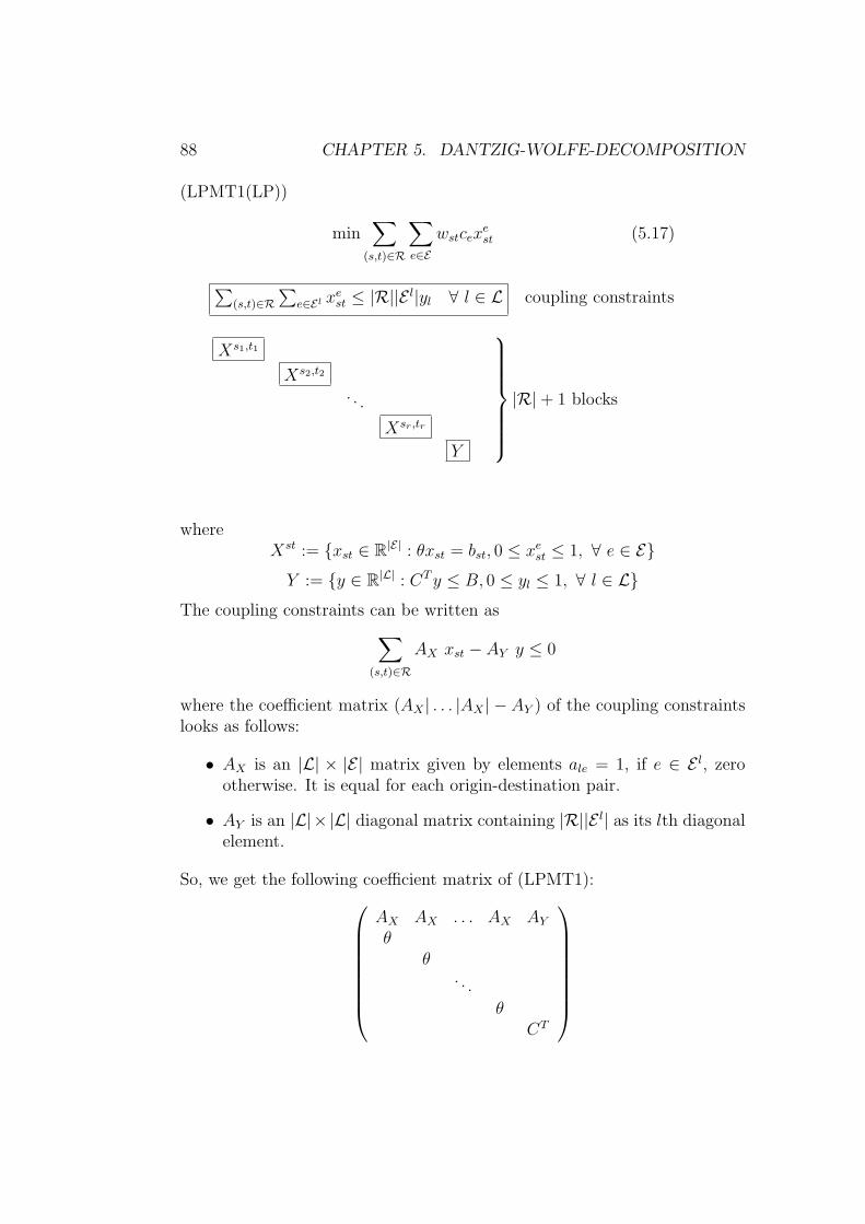
88 CHAPTER 5. DANTZIG-WOLFE-DECOMPOSITION
(LPMT1(LP))
min∑
(s,t)∈R
∑e∈E
wstcexest (5.17)
∑(s,t)∈R
∑e∈El xe
st ≤ |R||E l|yl ∀ l ∈ L coupling constraints
Xs1,t1
Xs2,t2
. . .
Xsr,tr
Y
⎫⎪⎪⎪⎪⎪⎪⎬⎪⎪⎪⎪⎪⎪⎭
|R| + 1 blocks
whereXst := {xst ∈ R
|E| : θxst = bst, 0 ≤ xest ≤ 1, ∀ e ∈ E}
Y := {y ∈ R|L| : CT y ≤ B, 0 ≤ yl ≤ 1, ∀ l ∈ L}
The coupling constraints can be written as∑(s,t)∈R
AX xst − AY y ≤ 0
where the coefficient matrix (AX | . . . |AX | − AY ) of the coupling constraintslooks as follows:
• AX is an |L| × |E| matrix given by elements ale = 1, if e ∈ E l, zerootherwise. It is equal for each origin-destination pair.
• AY is an |L|×|L| diagonal matrix containing |R||E l| as its lth diagonalelement.
So, we get the following coefficient matrix of (LPMT1):⎛⎜⎜⎜⎜⎜⎜⎜⎝
AX AX . . . AX AY
θθ
. . .
θCT
⎞⎟⎟⎟⎟⎟⎟⎟⎠
5.2. DANTZIG-WOLFE APPLIED ON (LPMT) 89
5.2.1 Master formulations
As we have seen in Section 5.1, the formulation of the Master Problem de-pends on the definition of the blocks. The blocks we have defined in formula-tion (5.17) is the finest decomposition we can think of. But it is also possibleto keep the budget constraint in the set of coupling constraints or to treatall shortest path blocks as one block. Thus, we can formulate four differentMaster Problems. Many others are also possible if we join not all but someshortest path blocks together to bigger blocks, e.g. for all (s, t) ∈ R startingat a given station s.In the following we define the weight-cost-parameters ce
st := wstce.
1. The Master Problem corresponding to the decomposition (5.17):
(Master 1)
z = min∑
(s,t)∈R
∑i
(cst x(i)st )αi
st (5.18)
s.t.∑
(s,t)∈R
∑i
(AX x(i)st )αi
st −∑
i
(AY y(i))βi + Iv = 0
∑i
αist = 1 ∀ (s, t) ∈ R
∑i
βi = 1
vl, αist, β
i ≥ 0
where the |L|-vector v are slack variables, and x(i)st and y(i) are the ex-
treme points of Xst, and Y , respectively. This problem has |L| couplingconstraints and |R| + 1 convexity constraints.
For each (s, t) ∈ R we obtain the following subproblem
zst = min(cst − πAX)xst − µst
s.t. xst ∈ Xst
The subproblem of the Y -block is
z = min(−πAY )y − µ00

90 CHAPTER 5. DANTZIG-WOLFE-DECOMPOSITION
s.t. yl ∈ Y,
where {πi}i∈L are the dual variables of the coupling constraints, {µst}(s,t)∈R
are the dual variables of the alpha convexity constraints and µ00 is thedual variable of the single beta convexity constraint.
Since the Xst blocks correspond to shortest path problems which areknown to be totally unimodular, the x
(i)st -values in {0, 1}|E|.
2. If we add the budget constraint to the set of coupling constraints, weget the following reformulation:
(LPMT1)
min∑
(s,t)∈R
∑e∈E
cestx
est (5.19)
∑(s,t)∈R
∑e∈l x
est ≤ |R||E l|yl ∀ l ∈ L∑
l∈L Clyl ≤ Bcoupling constraints
Xs1,t1
Xs2,t2
. . .
Xsr,tr
⎫⎪⎪⎪⎪⎬⎪⎪⎪⎪⎭
|R| blocks
The corresponding Master Program is:

5.2. DANTZIG-WOLFE APPLIED ON (LPMT) 91
(Master 2)
z = min∑
(s,t)∈R
∑i
(cst x(i)st )αi
st (5.20)
s.t.∑
(s,t)∈R
∑i
(AX x(i)st )αi
st − AY y + Iv = 0
∑l∈L
Clyl ≤ B
∑i
αist = 1 ∀ (s, t) ∈ R
vl, αist, yl ≥ 0
where the |L|-vector v are slack variables, and x(i)st are the extreme
points of Xst. This problem has |L| + 1 coupling constraints and |R|convexity constraints.
For each (s, t) ∈ R we obtain the same subproblems as for our firstformulation, namely
zst = min(cst − πAX)xst − µst
s.t. xst ∈ Xst
where {πi}i∈L are again the dual variables of the coupling constraints,and {µst}(s,t)∈R are the dual variables of the alpha convexity con-straints.
Again the Xst blocks correspond to shortest path problems which areknown to be totally unimodular, hence the x
(i)st -values are in {0, 1}|E|.
3. If we join the shortest path problems to one common block and thebudget constraint as a second block we get the following reformulation:

92 CHAPTER 5. DANTZIG-WOLFE-DECOMPOSITION
(LPMT1)
min∑e∈E
cexe (5.21)
∑e∈l x
e ≤ |R||E l|yl ∀ l ∈ L coupling constraints
X
Y
}2 blocks
with X := {x ∈ R|E| : xe =
∑(s,t)∈R xe
st ∀e ∈ E , xst ∈ Xst},
Y := {y ∈ R|L| : CT y ≤ B, 0 ≤ yl ≤ 1, ∀ l ∈ L}, and
ce :=∑
(s,t)∈R cest.
The corresponding Master Program is
(Master 3)
z = min∑
i
(c x(i))αi (5.22)
s.t.∑
i
(AX x(i))αi −∑
i
(AY y(i))βi + Iv = 0
∑i
αi = 1
∑i
βi = 1
vl, αi, βi ≥ 0
where the |L|-vector v are slack variables, and x(i) and y(i) are the ex-treme points of X, and Y , respectively. This problem has |L| couplingconstraints and only two convexity constraints.
The subproblem of the X-block is
z = min∑
(s,t)∈R
(cst − πAX)xst − µ

5.2. DANTZIG-WOLFE APPLIED ON (LPMT) 93
s.t. xst ∈ Xst
and xe :=∑
(s,t)∈R xest.
The subproblem of the Y -block is the same as for our first formulation:
z = min(−πAY )y − µ00
s.t. yl ∈ Y,
where {πi}i∈L are the dual variables of the coupling constraints, µ isthe dual variable of the alpha convexity constraint and µ00 is the dualvariable of the beta convexity constraint.
In this formulation the x(i)-values are integer because they are thecomponent wise sum over shortest path problem solution which arein {0, 1}.
4. If we add the budget constraint to the coupling constraints and treatthe Xst-blocks as one block we get the following reformulation:
(LPMT1)
min∑e∈E
cexe (5.23)
∑e∈l x
e ≤ |R||E l|yl ∀ l ∈ L∑l∈L Clyl ≤ B
coupling constraints
X 1 block
with X := {x ∈ R|E| : xe =
∑(s,t)∈R xe
st ∀e ∈ E , xst ∈ Xst} and
ce :=∑
(s,t)∈R cest.
The corresponding Master Program is:

94 CHAPTER 5. DANTZIG-WOLFE-DECOMPOSITION
(Master 4)
z = min∑
i
(c x(i))αi (5.24)
s.t.∑
i
(AX x(i))αi − AY y + Iv = 0
∑l∈L
Clyl ≤ B
∑i
αi = 1
vl, αi, yl ≥ 0
where the |L|-vector v are slack variables, and x(i) are the extremepoints of X. This problem has |L| + 1 coupling constraints and oneconvexity constraints.
The subproblem of the X-block is
z = min∑
(s,t)∈R
(cst − πAX)xst − µ
s.t. xst ∈ Xst
and xe :=∑
(s,t)∈R xest.
where {πi}i∈L are the dual variables of the coupling constraints, µ isthe dual variable of the alpha convexity constraint.
As in the previous formulation, the x(i)-values are again integer becausethey are the component wise sum over shortest path problem solutionwhich are in {0, 1}.
Table 5.1 summarizes the characteristics of the presented Master Programs:number of coupling constraints, number of convexity constraints and if theextreme points of the network flow problems are integer or {0, 1}.
So far, we only considered the possible decompositions and correspondingMaster programs of the (LPMT1) formulation. But what about the other

5.2. DANTZIG-WOLFE APPLIED ON (LPMT) 95
Master No. coupling convexity x(i)
1 |L| |R| + 1 {0, 1}2 |L| + 1 |R| {0, 1}3 |L| 2 integer4 |L| + 1 1 integer
Table 5.1: Characteristics of the Master programs of (LPMT1).
formulations?As we already mentioned, the extreme points of the X-subproblem of the(Master 3) and the (Master 4) are not {0, 1}, but integer. This is due tothe fact that we sum up the xe
st over all origin-destination pairs. By doingthis, we loose the information of the exact paths of the customers whichare needed in the (LPMT3), (LPMT4) and (LPMTF) formulation. So, itis easy to see that only (Master 1) and (Master 2) can be adapted to thesethree formulations, but (Master 3) and (Master 4) cannot. (LPMT2) canbe decomposed in all mentioned ways like the (LPMT1) without restrictionas the xe
st are summed up over all origin-destination pairs in its couplingconstraints, too.Table 5.2 summarizes our results.
Master 1 Master 2 Master 3 Master 4
(LPMT1) yes yes yes yes(LPMT2) yes yes yes yes(LPMT3) yes yes no no(LPMT4) yes yes no no(LPMTF) yes yes no no
Table 5.2: Possible masters for the different formulations
5.2.2 Strength of the Master Program
Since the original and the master formulation may differ in their linear pro-gramming relaxations, we will now discuss the strength of the linear pro-gramming masters introduced in this chapter.
Given the following integer program:

96 CHAPTER 5. DANTZIG-WOLFE-DECOMPOSITION
(P)
min cT x
s.t. Ax = b
x ≥ 0
x ∈ Zn
where A has block-angular structure:
Ax =
⎛⎜⎜⎜⎜⎜⎝
A0 A1 A2 · · · AK
B1
B2
. . .
BK
⎞⎟⎟⎟⎟⎟⎠
⎛⎜⎜⎜⎜⎜⎝
x0
x1
x2...
xK
⎞⎟⎟⎟⎟⎟⎠ =
⎛⎜⎜⎜⎜⎜⎝
b0
b1
b2...
bK
⎞⎟⎟⎟⎟⎟⎠
Then, the bound provided by the LP-relaxation of (P) is
zLP (P ) = min{cx :K∑
k=0
Akxk = b0,K∑
k=1
Bkxk = bk, xk ≥ 0}
Theorem 5.8. ([Wol98]) The bound provided by the corresponding Masterprogram (M) is
zLP (M) = min{K∑
k=0
ckxk :K∑
k=0
Akxk = b0, xk ∈ conv(Xk) ∀ k = 1 . . . K}
with Xk := {xk ∈ Nnk : Bkxk = bk}.
Proof. (M) can be obtained from the original problem (P) by substituting
xk =∑
i x(i)k λk,i with
∑i λk,i = 1, λk,i ≥ 0. This is equivalent to substituting
xk ∈ conv(Xk). �
This theorem tells us precisely how strong a bound is we obtain from theMaster.From integer programming theory (see e.g. [Wol98]), we know that
zLP (P ) ≤ zLP (M) ≤ zIP
where zIP is the integer solution value (zIP = zIP (P ) = zIP (M)).
In certain cases the bound provided by the Master has the same strength asthe linear programming relaxation.

5.2. DANTZIG-WOLFE APPLIED ON (LPMT) 97
If conv({xk ∈ Nnk : Bkxk = bk}) = {xk ∈ R
nk+ : Bkxk = bk} for all k = 1 . . . K
(i.e. if the current formulation of the subsystem already has the integralityproperty, that is, all extreme points of the current formulation are integral),then
zLP (P ) = zLP (M).
As we have mentioned, the shortest path blocks Xst in (LPMT) as well asthe corresponding network flow blocks in (LPMTF) are totally unimodularand thus have the integrality property. We hence get
zLP (LPMT ) = zLP (Master 2) = zLP (Master 4)
The same result holds for (LPMTF) with the corresponding Masters.
In our case the LP-relaxation of any formulation of (LPMT) is only solvablefor small instances, see Table 3.4. Since the LP-relaxation thus is not solvablefor real world instances due to the size of the resulting change&go network,a decomposition makes sense even if the provided bound is not better.
5.2.3 Initialization
In Section 5.1 we mentioned that we can use the solution of the subproblemsto generate an initial set of proposals and what to do if they violate thecoupling constraints.If in the case of the (LPMT) the solution of the subproblems satisfies thecoupling constraints, we know by Lemma 3.44 that these columns are alreadyoptimal. Thus, we only need to use the Dantzig-Wolfe approach, if the so-lution of the subproblems violates the coupling constraints which, using the(LPMT1) or (LPMT2) formulation scarcely appears. In this case, findinga feasible basic solution of the restricted Master program can be done in amuch more efficient way than a Simplex phase I procedure. It is also moreefficient since some commercial Simplex solvers do not offer a tool that re-turns the whole Simplex tableau after a solution is found. But in our casethe tableau is needed because we want to continue with a column generationprocedure. Theoretically this problem can be solved as we know the basis Bafter the Simplex I phase and thus only have to multiply our new columnswith B−1 but in real world instances our matrix gets huge and so computingthe inverse of it is too costly.
The way we tackle the problem is the following:We first convert our Master problem to the form

98 CHAPTER 5. DANTZIG-WOLFE-DECOMPOSITION
min cx
s.t. Ax = b
x ≥ 0
To this end we have to introduce non-negative slack variables with zero costfor all coupling constraints (v1, . . . , v|L|) and the budget constraint (vB). Theresult is that we nearly have an initial feasible basic solution. As only problemremain the convexity constraints which are equality constraints. For each ofthese rows we introduce also a non-negative slack variable vCr
with a veryhigh cost M (higher than the highest objective value of the shortest pathproblems, i.e. M >
∑(s,t)∈R
∑e∈E ce
st).
The resulting Simplex starting tableau of (Master 4) is
y1 . . . y|L| vB v1 . . . v|L| vC b
0 . . . 0 0 0 . . . 0 M 0C1 . . . C|L| 1 0 . . . 0 0 B
0 0 0
−AY
... I...
...0 0 0
0 . . . 0 0 0 . . . 0 1 1
respectively
y1 . . . y|L| vB v1 . . . v|L| vC b
0 . . . 0 0 0 . . . 0 0 -MC1 . . . C|L| 1 0 . . . 0 0 B
0 0 0
−AY
... I...
...0 0 0
0 . . . 0 0 0 . . . 0 1 1
with vB, v1 . . . v|L|, vC as feasible basic solution.
If we now add columns and solve the new Master to get the dual variables, wehave to keep in mind to subtract M from the dual of the convexity constraintbefore adjusting the subproblem with it.

5.3. COMPUTATIONAL RESULTS 99
Decomposition No. 0 No. 1 No. 13LP relax 0.01 M MMaster 1 0.19 M MMaster 2 0.15 M MMaster 3 0.12 4 17318Master 4 0.1 1 8715
Table 5.3: CPU times of the LP-relaxation of (LPMT1) using Dantzig-Wolfe
approach with different Masters. Instances are explained in Table 3.2. M denotes
”out of memory”.
5.3 Computational results
We implemented the Dantzig-Wolfe decomposition approach of (LPMT) us-ing Xpress MP 2003 and Microsoft Visual C++ 6.0. The CPU times of thissection are based on a 3.06 GHz Intel4 processor with 512 MB RAM.Our computational experience shows that the (Master 4) variation of the(LPMT1) while solving the subproblem with Dijkstra’s shortest path algo-rithm finds an optimal solution of the LP-relaxation within minutes. Even forthe biggest instance a solution was found in less than three hours. Note thatline planning is part of the strategic planning level and so even longer com-putation times of some hours are acceptable. In general only few iterationsare needed.
5.3.1 Variations of the Decomposition
First, we implemented the Dantzig-Wolfe decomposition algorithm for allfour Masters for (LPMT1). Table 5.3 shows the CPU times for some selectedinstances. Row ”‘LP relax”’ repeats the computation times solving the LP-relaxation using standard optimization software. Note, that the computationtimes in this section are based on a machine with less memory than thesolutions presented in the rest of this thesis, namely 512 MB instead of 2 GBRAM.Our computational experience shows that it is better for solving the completeproblem if the budget constraint belongs to the coupling constraints (i.e.(Master2) and (Master4)). This is, because it is only one constraint andits variables do not appear in the objective function. Thus, we only needa feasible solution and solving the corresponding subproblem to optimalitytakes unnecessary computation time.Normally it is known to be better to split the remaining constraints into as

100 CHAPTER 5. DANTZIG-WOLFE-DECOMPOSITION
many blocks as possible in order to reduce the number of iterations and thusthe computation time. Of course, the number of convexity constraints in theMaster problem increases but since the structure of the convexity constraintsis very simple, modern optimization software can manage them easily. In ourcase, the number of convexity constraints increases enormously if we treat theXst-blocks individually, namely in (Master1) and (Master2), and so memoryproblems arise even for small instances. On the other hand, we figured outthat even if we treat the shortest path problems as one subproblem and thusonly have one convexity constraint, we only need very few iterations suchthat there is no need for further decomposition.With regard to the Ti-values of Table 3.5, we are mainly interested in thesolution of the LP-relaxation of (LPMT3) and (LPMT4). With our know-ledge about the inefficiency of treating the budget constraint as a separateblock, we implemented the Dantzig-Wolfe approach for these two formula-tions using (Master2) (remember, that there is no (Master4) for them, seeTable 5.2). Unfortunately, even using the Dantzig-Wolfe approach, it is notpossible to solve even small instances of (LPMT4). Whereas (LPMT3) couldbe solved for instances up to 116 lines and 16274 origin-destination pairs (seeTable 5.4).
5.3.2 Variations of the line pool
As already specified, the problem size and thus the CPU time depends mainlyon the size of the line pool and on the number of origin-destination pairs (seee.g. Table 3.3). We calculated the 14 instances of Table 3.2 to show thedependency between the running time and the line pool size. As we alreadymentioned, we always used the same origin-destination matrix, but to avoidinfeasibility we deleted such origin-destination pairs that could not be servedeven if all lines of the line pool were used. The remaining number of elementsof R is shown in Table 5.4 in column ”|R|”.In column ”CPU1”, we show the CPU time of an implementation of (LPMT1)with (Master4). Since we only need very few iterations, we can save a lotof running time by checking whether the π change in comparison to thelast iteration or not after solving the subproblems. If not, there is no needto recalculate the shortest paths in the next iteration since no distanceswill change. In this case, we just have to adjust the last objective valueby −µ. The CPU times of this variation are shown in Table 5.4 in column”CPU1 check” for (LPMT1) with (Master 4) and in column ”CPU3 check” for(LPMT3) with (Master 2). In all implementations we solved the subproblemsby Dijkstra’s algorithm.Figure 5.2 shows graphically the results of Table 5.4.
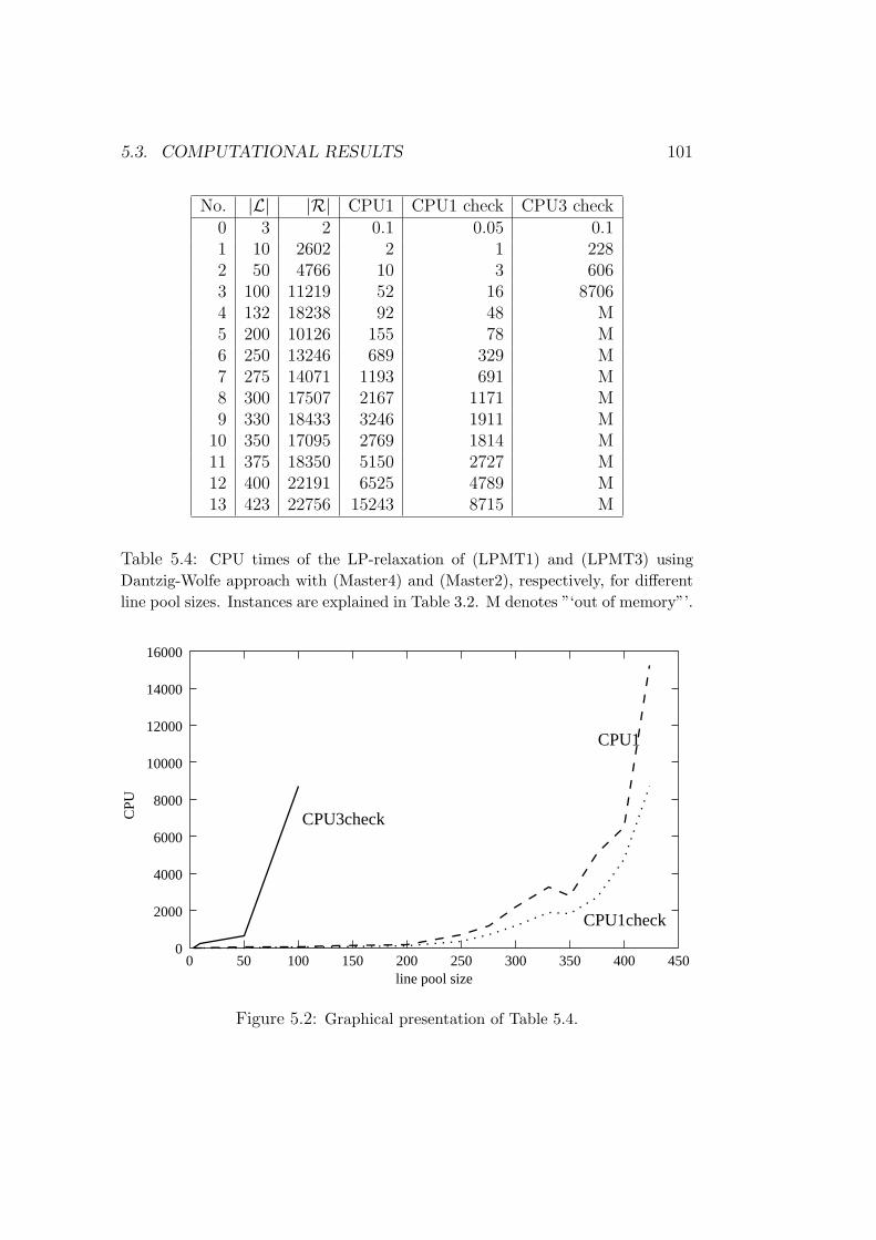
5.3. COMPUTATIONAL RESULTS 101
No. |L| |R| CPU1 CPU1 check CPU3 check0 3 2 0.1 0.05 0.11 10 2602 2 1 2282 50 4766 10 3 6063 100 11219 52 16 87064 132 18238 92 48 M5 200 10126 155 78 M6 250 13246 689 329 M7 275 14071 1193 691 M8 300 17507 2167 1171 M9 330 18433 3246 1911 M
10 350 17095 2769 1814 M11 375 18350 5150 2727 M12 400 22191 6525 4789 M13 423 22756 15243 8715 M
Table 5.4: CPU times of the LP-relaxation of (LPMT1) and (LPMT3) using
Dantzig-Wolfe approach with (Master4) and (Master2), respectively, for different
line pool sizes. Instances are explained in Table 3.2. M denotes ”‘out of memory”’.
CPU3check
CPU1
CPU1check
0
2000
4000
6000
8000
10000
12000
14000
16000
0 50 100 150 200 250 300 350 400 450
CPU
line pool size
Figure 5.2: Graphical presentation of Table 5.4.

102 CHAPTER 5. DANTZIG-WOLFE-DECOMPOSITION

Chapter 6
Exact solution method
We are now in a position to present an exact solution method of the line plan-ning problem with minimal transfers. This method is based on a branch andbound procedure with the LP-relaxation of one of the (LPMT) formulationsas upper bounds. The choice of the formulation depends on the size of thenetwork. The bounds can be often calculated in polynomial time by usingLemma 3.44. If this lemma fails we calculate them by using the Dantzig-Wolfe procedure presented in Section 5.2. Note that the xe
st variables arealways in {0, 1} since they represent the solution of a shortest path problem.So, we only have to branch along the yl variables. Since they are {0, 1} vari-ables and the number of 1s is bounded by the budget, the enumeration treeitself is relatively small.
6.1 Branch & Bound
The most common way to solve integer programs is to use implicit enumer-ation, or branch & bound, in which linear programming relaxations providethe bounds.
Main steps in the branch & bound method:
1. Selecting a subproblem.
2. Relax the subproblem: For each of the subproblems, we need to obtaina bound on how good its best feasible solution can be. This is usuallydone by solving a relaxation of the problem. For integer programmingproblems, the most widely used relaxation is the linear programmingrelaxation. We can also use other kinds of relaxations, for exampleLagrangian relaxation or Dantzig-Wolfe decomposition. In our case
103

104 CHAPTER 6. EXACT SOLUTION METHOD
these three possibilities lead to the same bounds (see Section 5.2.2 and[Wol98], Theorem 10.3)
3. Pruning: Pruning or terminating is done partially by using the boundto discard a subproblem from further investigation. A subproblem Pis pruned if one of the following cases happens:
(a) Pruning by infeasibility: The relaxation of P has no feasible solu-tion.
(b) Pruning by bound: The optimal objective value of the relaxationof P is not better than the objective value of the best feasiblesolution found so far.
(c) Pruning by optimality: The optimal solution for the relaxation ofP is integer.Note that if this solution gives better objective value than thecurrent best solution, it becomes the new best solution.
4. Branching: The branching is done by dividing the original problem intosmaller subproblems. The optimal solution of the relaxed problem willbe cut away through the branching.
The general form of the branch & bound algorithm for binary programs (BIP)is:
Algorithm 6.1. Branch & Bound Algorithm for binary programs
1. Initialization. Set z = ∞, list = {(BIP )}, n=0.
2. Select subproblem Pk from list. Solve the relaxation of this subproblemPk. We denote the solution by xPk and the objective value by zPk
. zPK
gives a lower bound on subproblem Pk.
3. Pruning by infeasibility: If there is no feasible solution to Pk, goto Step7.
4. Pruning by bound: If zPk≥ z, goto Step 7.
5. Pruning by optimality: If xPk is an integer feasible solution, set z := zPk
and x := xPk , goto Step 7.
6. Branch on a variable xj whose value is not integer by fixing the variableat value either 0 or 1. We obtain two new subproblems Pn+1 and Pn+2.Set list = list ∪ {Pn+1, Pn+2} and n := n + 2. Goto Step 2.

6.2. BRANCH & BOUND APPLIED ON (LPMT) 105
7. Set list = list \ {Pk}.Optimality test: If list = ∅, stop: the current best solution x withobjective value z is optimal to the original (BIP). Otherwise goto Step2.
6.2 Branch & Bound applied on (LPMT)
As the size of the change&go network and thus the size of the model for-mulation is huge in real world instances, it is in general not possible tocalculate the LP-relaxation using standard optimization software (see Table3.4). Therefore, we developed in this thesis two other ways to calculate theLP-relaxation:
1. Using the trivial solution if Lemma 3.44 holds.
2. Using Dantzig-Wolfe decomposition if Lemma 3.44 does not hold.
We will now show the Branch & Bound algorithm using the (LPMT1) andthe (LPMT3) formulation:
Example 6.2. We consider the PTN shown in Figure 6.1 together with the
3
1 2
4
Figure 6.1: PTN of Example 6.2.
line pool
L := {(l1, l2, l3, l4} = {(1, 2, 3), (2, 4, 3), (1, 3, 4), (1, 3)}
and the origin-destination pairs
R := {(1, 3), (1, 4), (2, 3)}

106 CHAPTER 6. EXACT SOLUTION METHOD
The edge costs for the driving edges are 1 and the costs of the changing edgesare 4. The line costs are set to 1 for all lines and the budget is 2.A trivial solution is: customer (1, 3) uses l4 (or l3), customer (1, 4) uses l3and customer (2, 3) uses l1. Using Lemma 3.44, we get the following T-values representing the minimal budget such that the trivial solution still isthe optimal solution of the LP-relaxation of the corresponding formulation:
T1 =1
6+
0
6+
2
6+
1
3=
5
6< 2
T2 =1
3+
0
3+
1
3+
1
3= 1 < 2
T3 =1
2+
0
2+
2
2+
1
1=
5
2> 2
T4 = 1 + 0 + 1 + 1 = 3 > 2
We see, that the trivial solution can be used as LP-relaxation for the (LPMT1)and the (LPMT2) formulation, but not for the (LPMT3) and the (LPMT4)formulation. For these, the relaxation must be calculated using Dantzig-Wolfe decomposition or, as it is still possible in this small example, usingstandard optimization software.
We will now show the branch & bound algorithm for the (LPMT1) and the(LPMT3) formulation.
1. (LPMT1):Since the xe
st-values are always integer, it is sufficient to consider onlythe yl variables. The LP-relaxation solution of the original problem is
y(0) = (0.17, 0, 0.33, 0.33), z(0) = 4
Since this solution is fractional (yl1 = 0.17), our next step is to parti-tion (branch) the original set of feasible solutions into subsets by fixingthe value of the variable yl1 at yl1 = 0 for one subset and at yl1 = 1for the other subset. Thus, the original problem is divided into twosmaller subproblems as follows:Subproblem 1: (yl1 = 0)
min∑
(s,t)∈R
∑e∈E
wst ce xest

6.2. BRANCH & BOUND APPLIED ON (LPMT) 107
s.t.∑
(s,t)∈R
∑e∈El
xest ≤ |R||E l|yl ∀ l ∈ L
θxst = bst ∀ (s, t) ∈ R∑l∈L
Clyl ≤ B
yl1 = 0
xest, yl ∈ B ∀ (s, t) ∈ R, e ∈ E , l ∈ L
which is equivalent to:
min∑
(s,t)∈R
∑e∈E
wst ce xest
s.t.∑
(s,t)∈R
∑e∈El
xest ≤ |R||E l|yl ∀ l ∈ L \ {l1}
∑(s,t)∈R
∑e∈El1
xest = 0
θxst = bst ∀ (s, t) ∈ R∑l∈L\{l1}
Clyl ≤ B
xest, yl ∈ B ∀ (s, t) ∈ R, e ∈ E , l ∈ L
which is equivalent to solve (LPMT) with a new line pool L∗ := L\{l1}.
Subproblem 2: (yl1 = 1)
min∑
(s,t)∈R
∑e∈E
wst ce xest

108 CHAPTER 6. EXACT SOLUTION METHOD
s.t.∑
(s,t)∈R
∑e∈El
xest ≤ |R||E l|yl ∀ l ∈ L
θxst = bst ∀ (s, t) ∈ R∑l∈L
Clyl ≤ B
yl1 = 1
xest, yl ∈ B ∀ (s, t) ∈ R, e ∈ E , l ∈ L
which is equivalent to:
min∑
(s,t)∈R
∑e∈E
wst ce xest
s.t.∑
(s,t)∈R
∑e∈El
xest ≤ |R||E l|yl ∀ l ∈ L \ {l1}
∑(s,t)∈R
∑e∈El1
xest ≤ |R||E l1| redundant!
θxst = bst ∀ (s, t) ∈ R∑l∈L\{l2}
Clyl ≤ B − Cl1
xest, yl ∈ B ∀ (s, t) ∈ R, e ∈ E , l ∈ L
which is equivalent to the original problem with slightly changed budget
constraint.

6.2. BRANCH & BOUND APPLIED ON (LPMT) 109
It is easy to see that the developed solution methods of the LP-relaxationalso work for the subproblems. Solving the LP-relaxation of subprob-lem 1 and 2 using Lemma 3.44, which has to be adapted for subproblem2 to
T1 :=∑
l∈L\{l1}
Cl
T1l
|R||E l|=
1
3≤ 1 = B − Cl1
yields their optimal solutions:
y(1) = (0, 0.33, 0.5, 0), z(1) = 5
y(2) = (1, 0, 0.5, 0), z(2) = 4
Both solutions are feasible and the objective values are smaller thanthe current best upper bound z = ∞.Now we have to choose a selection-rule to decide which subproblemshould be branched next. We could do the best first search and choosethe subproblem with the currently best lower bound z or we could dothe breadth first search and discharge a whole level of a tree before go-ing deeper or we could do the depth first search and continue in onedirection until all variables are fixed. We will use the depth first searchin this example.
So, we branch subproblem 1 and get subproblem 3 by fixing yl2 = 0.Solving subproblem 3, we find no feasible solution. This is obvioussince there is no more line serving station 2 if we forbid lines l1 and l2.We now go back to subproblem 1 and get subproblem 4 by fixing yl2 = 1whose objective value is 5 and thus still better than the best feasiblesolution found so far. Note that if we fix a variable to 1 it is sufficient tocheck if the last solution still works with the new budget constraint. Ifit is so, this is an optimal solution to the new subproblem. Otherwise,we have to do the Dantzig-Wolfe approach.
The solution procedure of the Branch & Bound method for these twoiterations can be described by a tree search which is shown in Figure6.2. The nodes of this tree represent the subproblem (node 0 representsthe original problem) and the edges specify how variables are fixed inthe solution process. At edge {0, 1} and {0, 2}, the value of yl1 is spec-ified. This variable is referred to as fixed variable. All variables whosevalues are unspecified at a node are called free variables. The numbersin the nodes indicate the sequence in which the subproblems have beeninvestigated. The numbers at the nodes are the optimal solutions with

110 CHAPTER 6. EXACT SOLUTION METHOD
z0=4y0=(0.17,0,0.33,0.33)
y_1=1
1 2
y4=(0,1,0.5,0)
z4=5
0
3
infeasible
y_2=0
y_1=0
y_2=1
y2=(1,0,0.5,0)z2=4z1=5
y1=(0,0.33,0.5,0)
4
Figure 6.2: The Branch & Bound tree after two iterations.
their objective values of the LP-relaxation of the subproblem. This treecontinues ”growing branches” iteration by iteration. It is referred to asthe branch and bound tree.
Figure 6.1 shows the complete branch and bound tree of the example.
Subproblem 5 yields the first integer solution. In this step the upperbound is set to z = 9, because it is the currently best feasible solution.In subproblem 6, we get again an integer solution with a better objec-tive value than 9, so we set z = 5 and store this solution as currentlybest solution. With this problem, searching for solutions with yl1 = 0ends and we continue branching subproblem 2. In subproblem 7 wefind a feasible solution of the LP-relaxation of the subproblem with anobjective value bigger than z and so we can stop branching this prob-lem because we won´t find a better solution in this branch (pruning bybound). Finally in subproblem 8 we find the optimal solution.
Note that in this example the depth first rule was not applied conse-quently, since subproblem 2 was treated before subproblem 6. This wasdone to show in the beginning of the example how both kinds of sub-problems are build. The correct sequence of subproblems using depthfirst search would be 0,1,3,4,5,6,2,7,8.
2. (LPMT3):

6.3. PREPROCESSING 111
z0=4y0=(0.17,0,0.33,0.33)
y_1=1
1 2
y4=(0,1,0.5,0) y7=(1,0.17,0,0.33)
z4=5 z7=8 z8=4
z5=9
0
3 4
5 6
7 8
infeasible
y_2=0
y_1=0
y_3=0
y_2=1 y_3=1
y_3=1
y_3=0
y8=(1,0,1,0)
y2=(1,0,0.5,0)z2=4
y6=(0,1,1,0)
z6=5
y5=(0,1,0,1)
z1=5y1=(0,0.33,0.5,0)
Figure 6.3: The complete Branch & Bound tree (LPMT1).
If we use the (LPMT3) formulation, solving the LP-relaxation is harderbecause the trivial solution is not feasible. But on the other hand, thebounds provided by this formulation are much better and so the branchand bound tree is much smaller as we can see in Figure 6.4 that showsthe complete branch and bound tree of this example.
Concluding, we can say, that the number of iterations, i.e. the size of thetree, depends on the strength of the formulation used, but as we have seenin Section 5.3, the better the strength of a formulation, the harder it is tosolve the LP-relaxation.
6.3 Preprocessing
As we have seen, the main problem of our approach is the size of the change&gonetwork whose size depends mainly on the size of the line pool. A wise choiceof a possibly small line pool is therefore advisable. On the other hand it makessense to analyze the underlying PTN. For example if two lines go parallel for

112 CHAPTER 6. EXACT SOLUTION METHOD
z0=4
y_1=1
1 2
0
y2=(1,0,1,0)y1=(0,1,1,0)z1=5 z2=4
y0=(0.5,0,1,0)
y_1=0
Figure 6.4: The complete Branch & Bound tree (LPMT3).
a long time, it is sufficient to add changing arcs only at the first and thelast station. Also arcs between stations without changing possibility can beshrunken together to decrease the size of the network.

Chapter 7
Conclusions
In this thesis we investigated both, the mathematical and the practical as-pects of the line planning problem. First, we reviewed some existing ap-proaches of customer and cost oriented line planning problems.
In Chapter 3 we developed a new customer oriented line planning problem(LPMT) that minimizes the total travel time of the customers includingpenalties for transfers needed. For this, we extended the given public trans-portation network to a new network, the so-called change&go-network. Thechoice of its edge costs provides a wide variety of objectives, beginning from”count transfers” with the reduced line-change-network up to the possibilityto forbid or to favor special stations for transfers, e.g. because of their in-frastructure.We presented four binary programming formulations (LPMTi), i = (1, . . . , 4)for (LPMT) and have shown their equivalence. Furthermore, we discussedbicriteria formulations of (LPMT) and have shown that applying the ε-constrained method for finding the efficient solutions of the problem is equalto our single-objective binary programming formulations if we set the ε to agiven budget. Finally, we extended our model to include frequencies of thelines and presented an integer programming formulation for this extension.
We continued with a discussion of the strength of the bounds provided bythe LP-relaxation of our four binary, single-objective formulations and fig-ured out that in some special cases the trivial solution which can be found inpolynomial time is equal to the solution of the LP-relaxation. Computationalresults have shown that for some of the formulation this special case oftenappears. If the trivial solution is infeasible, we have to find other ways tofind a solution of the LP-relaxation. In real world instances it is not possibleto use standard optimization software due to the problem size. Therefore, in
113

114 CHAPTER 7. CONCLUSIONS
Chapter 5, we took advantage of the block diagonal structure of the (LPMTi)formulations and proposed an Dantzig-Wolfe decomposition approach. Thesubproblems turned out to be shortest path problems which can be solvedby efficient algorithms and thus the problem was solvable even for large real-world instances of long distance trains of German Railway within less thantwo hours.
Finally, in Chapter 6 we proposed a branch & bound procedure to find an ex-act solution. As lower bound, we used the solution value of the LP-relaxationwhich can be found by the trivial solution or if it is infeasible by the Dantzig-Wolfe approach.
Another way to tackle our problem was based on heuristics. In Chapter 4 wepresented and discussed various different heuristics and heuristic ideas. Oneof them, namely the line segment heuristic, plays a special role since it isthe only method in this thesis that constructs lines instead of choosing themfrom a set of possible lines. This approach will soon be subject of a projectwork at the Georg-August University of Gottingen.

List of Symbols
Public transportation network:PTN = (S,E) . . . . . . . . . . . . . . . . . . . . . . . . . . . . . . public transportation networkS . . . . . . . . . . . . . . . . . . . . . . . . . . . . . . . . . . . . . . . . . . . . . . . . . . . . . . . . . . . set of stationsE . . . . . . . . . . . . . . . . . . . . . . . . . . . . . . . . . . . . . . . . . . . . . . . . . . . . . . . set of direct rideste . . . . . . . . . . . . . . . . . . . . . . . . . . . . . . . . . . . . . . . . . . . . . . . . . . . driving time of edge e
Passengers demand:R . . . . . . . . . . . . . . . . . . . . . . . . . . . . . . . . . . . . . . . . . . . set of origin-destination pairswst . . . . . . . . . . . . . . . . . . . . . . . . . . . . . number of customers traveling from s to t
Line Planning:l . . . . . . . . . . . . . . . . . . . . . . . . . . . . . . . . . . . . . . . . . . . . . . . . . . . . . . . . . . . . . . . . . . . . . . lineE(l) . . . . . . . . . . . . . . . . . . . . . . . . . . . . . . . . . . . . . . . .set of edges belonging to line lS(l) . . . . . . . . . . . . . . . . . . . . . . . . . . . . . . . . . . . . . set of stations belonging to line lL . . . . . . . . . . . . . . . . . . . . . . . . . . . . . . . . . . . . . . . . . line concept without frequencies(L, f) . . . . . . . . . . . . . . . . . . . . . . . . . . . . . . . . . . . . . . . . line concept with frequenciesL . . . . . . . . . . . . . . . . . . . . . . . . . . . . . . . . . . . . . . . . . . . . . . . . . . . . . . . . . . . . . . . . line poolfl . . . . . . . . . . . . . . . . . . . . . . . . . . . . . . . . . . . . . . . . . . . . . . . . . . . . . . . frequency of line lf(e) . . . . . . . . . . . . . . . . . . . . . . . . . . . . . . . . . . . . . . . . . . . . . . . . . . . frequency of edge efmin
e , fmaxe . . . . . . . . . . . . . . . . . . . . . . . minimum, maximum frequency of edge e
Cl . . . . . . . . . . . . . . . . . . . . . . . . . . . . . . . . . . . . . . . . . . . . . . . . . . . . . . . . . . . . cost of line lL(s) . . . . . . . . . . . . . . . . . . . . . . . . . . . . . . . . . set of lines passing through station s
Change&go-network:GCG = (V , E) . . . . . . . . . . . . . . . . . . . . . . . . . . . . . . . . . . . . . . . . .Change&go-networkV . . . . . . . . . . . . . . . . . . . . . . . . . . . . . . . . . . . . . . . . . . . . . . . . . . . . . . . . . . . . . set of nodesVCG . . . . . . . . . . . . . . . . . . . . . . . . . . . . . . . . . . . . . . . . . . set of station-line-pair-nodesVOD . . . . . . . . . . . . . . . . . . . . . . . . . . . . . . . . . . . . . . . . . . . . . . . . . . . set of in/out-nodesE . . . . . . . . . . . . . . . . . . . . . . . . . . . . . . . . . . . . . . . . . . . . . . . . . . . . . . . . . . . . . set of edgesEchange . . . . . . . . . . . . . . . . . . . . . . . . . . . . . . . . . . . . . . . . . . . . . . . set of changing edgesE l . . . . . . . . . . . . . . . . . . . . . . . . . . . . . . . . . . . . . . . . . . . . .set of driving edges of line l
115

116 CHAPTER 7. CONCLUSIONS
Ego . . . . . . . . . . . . . . . . . . . . . . . . . . . . . . . . . . . . . . . . . . . . . . . . . . . . set of driving edgesEOD . . . . . . . . . . . . . . . . . . . . . . . . . . . . . . . . . . . . . . . . . . . . . . . . . . . . set of in/out-edgesE(L) . . . . . . . . . . . . . . . . . . . . . . . . . edge set of GCG constructed of the lines of Lce . . . . . . . . . . . . . . . . . . . . . . . . . . . . . . . . . . . . . . . . . . . . . . . . . . . . . . . . . . . cost of edge eceOD
. . . . . . . . . . . . . . . . . . . . . . . . . . . . . . . . . . . . . . . . . . . . . . . . cost of an in/out-edgeθ . . . . . . . . . . . . . . . . . . . . . . . . . . . . . . . . . . . . . . . .node-arc-incidence matrix of GCG
B . . . . . . . . . . . . . . . . . . . . . . . . . . . . . . . . . . . . . . . . . . . . . . . . . . . . . . . . . . . . . . . . . .budget(x, yi) . . . . . . . . . . . . . . . . . . . . . . . . . . .trivial solution of (LPMTi), i ∈ {1, . . . , 4}Ti . . . . . . . . . . . . . . . . . . . . . . . . . . . . . minimal budget such that (x, yi) is feasiblex(L) . . . . . . . . . . . . . . . . . . . . . . . . . . . . . . . . . . . . . . . . . . . . . . . solution of (LPMT(L))
Set of numbers:Z . . . . . . . . . . . . . . . . . . . . . . . . . . . . . . . . . . . . . . . . . . . . . . . . . . .set of integer numbersR . . . . . . . . . . . . . . . . . . . . . . . . . . . . . . . . . . . . . . . . . . . . . . . . . . . . . .set of real numbersB . . . . . . . . . . . . . . . . . . . . . . . . . . . . . . . . . . . . . . . . . . . . . . . . . . . . . . . . . . . . . . . . . . . {0, 1}N . . . . . . . . . . . . . . . . . . . . . . . . . . . . . . . . . . . . . set of non-negative integer numbers

List of Figures
2.1 The network with the main stations of long-distance trains in Ger-
many. [Rai] . . . . . . . . . . . . . . . . . . . . . . . . . . . . . 20
3.1 Difference between the objectives ”maximize direct travelers” and
”minimize transfers”. . . . . . . . . . . . . . . . . . . . . . . . . 233.2 Solution ”maximize direct traveler”. . . . . . . . . . . . . . . . . 243.3 Solution ”minimize transfers”. . . . . . . . . . . . . . . . . . . . 243.4 Construction of the line planning problem in the proof of Theorem
3.8. . . . . . . . . . . . . . . . . . . . . . . . . . . . . . . . . . 283.5 The public transportation network of Example 3.11. . . . . . . . . 313.6 The change&go graph of Example 3.11. . . . . . . . . . . . . . . 313.7 The shrunken line-change-network of Figure 3.6 in the special case:
”Customers only count transfers”. . . . . . . . . . . . . . . . . . 323.8 Efficient solutions of bicriteria optimization problem. . . . . . . . 383.9 Two alternative formulations for the same integer set proposed in
Example 3.11. . . . . . . . . . . . . . . . . . . . . . . . . . . . 433.10 P3 is a better formulation of the integer set of Example 3.11 than
P1 and P2, but not ideal. . . . . . . . . . . . . . . . . . . . . . 473.11 P3 is the ideal formulation of the integer set of Example 3.11. . . . 483.12 The change&go graph of Example 3.11. . . . . . . . . . . . . . . 493.13 path combination: alternative A. . . . . . . . . . . . . . . . . . . 503.14 path combination: alternative B. . . . . . . . . . . . . . . . . . . 513.15 Schematical summary of the results of Section 3.4. . . . . . . . . . 533.16 Block diagonal matrix structure, (a) with coupling constraints, (b)
with coupling variables, and (c) with coupling constraints and vari-
ables. Only the shaded regions may contain non-zero elements. . . 543.17 Line pool of Example 3.45. . . . . . . . . . . . . . . . . . . . . . 59
4.1 Joining lines in the line segment heuristic. . . . . . . . . . . . . . 754.2 CPU times of different heuristics. . . . . . . . . . . . . . . . . . 774.3 Objective values of different heuristics. . . . . . . . . . . . . . . . 77
117

118 LIST OF FIGURES
5.1 Communication between restricted master and subproblems. . . . 855.2 Graphical presentation of Table 5.4. . . . . . . . . . . . . . . . . 101
6.1 PTN of Example 6.2. . . . . . . . . . . . . . . . . . . . . . . . . 1056.2 The Branch & Bound tree after two iterations. . . . . . . . . . . 1106.3 The complete Branch & Bound tree (LPMT1). . . . . . . . . . . 1116.4 The complete Branch & Bound tree (LPMT3). . . . . . . . . . . 112

List of Tables
2.1 Instances for different line pool sizes . . . . . . . . . . . . . . . . 19
3.1 The line pool of example 3.5. . . . . . . . . . . . . . . . . . . . . 233.2 Instances for different line pool sizes . . . . . . . . . . . . . . . . 303.3 CPU times for the LP-relaxation of (LPMT1) for different line pool
sizes and origin-destination sets. ”‘M”’ denotes out of memory. . . 563.4 CPU times for the LP-relaxation of the four formulations using
XpressMP, ”M” denotes out of memory) . . . . . . . . . . . . . . 563.5 Minimal budgets such that trivial solution is optimal solution of
the LP-relaxation of the different formulations of the (LPMT), see
Lemma 3.44. CPU times in seconds. . . . . . . . . . . . . . . . . 58
4.1 Solutions of the cover greedy algorithms for different line pool sizes 684.2 Solutions of the list greedy algorithms for different line pool sizes . 694.3 Delete OD-heuristics for different line pool sizes . . . . . . . . . . 724.4 Delete path-heuristics for different line pool sizes . . . . . . . . . 72
5.1 Characteristics of the Master programs of (LPMT1). . . . . . . . 955.2 Possible masters for the different formulations . . . . . . . . . . . 955.3 CPU times of the LP-relaxation of (LPMT1) using Dantzig-Wolfe
approach with different Masters. Instances are explained in Table
3.2. M denotes ”out of memory”. . . . . . . . . . . . . . . . . . 995.4 CPU times of the LP-relaxation of (LPMT1) and (LPMT3) us-
ing Dantzig-Wolfe approach with (Master4) and (Master2), respec-
tively, for different line pool sizes. Instances are explained in Table
3.2. M denotes ”‘out of memory”’. . . . . . . . . . . . . . . . . . 101
119

120 LIST OF TABLES

Bibliography
[Abr98] T. Abrahamsson, Estimation of origin-destination matrices usingtraffic count - a literature survey., Technical report Interim Re-port IR98-021, International Institute for Applied System Analy-sis, Laxenburg, Austria, 1998.
[BGP04] R. Borndorfer, M. Grotschel, and M.E. Pfetsch, Models for lineplanning in public transport, ZIP-Report 04-10, Konrad-Zuse-Zentrum fur Informationstechnik Berlin, 2004.
[BKZ96] M.R. Bussieck, P. Kreuzer, and U.T. Zimmermann, Optimal linesfor railway systems, European Journal of Operational Research96 (1996), no. 1, 54–63.
[BLL03] M.R. Bussieck, T. Lindner, and M.E. Luebbecke, A fast algo-rithm for near cost optimal line plans, Tech. Report 2003/43,Technische Universitat Berlin, 2003.
[BLL04] M.R. Bussieck, T. Lindner, and M.E. Lubbecke, A fast algorithmfor near cost optimal line plans, mathematical methods of oper-ational research 59 (2004), no. 2, 205–220.
[Bus98] M.R. Bussieck, Optimal lines in public transport, Ph.D. thesis,Technische Universitat Braunschweig, 1998.
[BZ97] M.R. Bussieck and U.T. Zimmermann, Schlußbericht - Opti-male Linienfuhrung und Routenplanung in Verkehrssystemen(Schienenverkehr), 1997.
[Car94] M. Carey, A model and strategy for train pathing with choiceof lines, platforms, and routes, Tranportation Res. Part B 28(1994), no. 5, 333–353.
[Cla94] M.T. Claessens, De kost-lijnvoering, Master’s thesis, Universityof Amsterdam, 1994.
121

122 BIBLIOGRAPHY
[CvDZ98] M.T. Claessens, N.M. van Dijk, and P.J. Zwaneveld, Cost opti-mal allocation of rail passenger lines, European Journal on Op-erational Research 110 (1998), no. 3, 474–489.
[Die78] H. Dienst, Linienplanung im spurgefuhrten Personenverkehr mitHilfe eines heuristischen Verfahrens, Ph.D. thesis, TechnischeUniversitat Braunschweig, 1978.
[DW60] G.P. Dantzig and P. Wolfe, Decomposition principle for linearprograms, Operations Research 8 (1960), 101–111.
[Ehr00] M. Ehrgott, Multiple criteria optimization, Lecture Notes in Eco-nomics and Mathematical Systems, vol. 491, Springer, Berlin,2000.
[FW81] P.G. Furth and N.H.M. Wilson, Setting frequencies on busroutes: Theory and practice, Transportation Research Record818 (1981), 1–7.
[Goo04] J.-W. Goossens, Models and algorithms for railsway line planningproblems, Ph.D. thesis, University of Maastricht, 2004.
[GvHK02] J.-W. Goossens, C.P.M. van Hoesel, and L.G. Kroon, On solv-ing multi-type line planning problems, Tech. Report RM/02/009,University of Maastricht, 2002, METEOR Research Memoran-dum.
[GvHK04] J.-W. Goossens, S. van Hoesel, and L.G. Kroon, A branch-and-cut approach for solving railway line-planning problems., Trans-portation Science 38 (2004), no. 3, 379–393.
[HC83] Y.Y. Haimes and V. Chankong, Multiobjective decision making— theory and methodology, North Holland, New York, 1983.
[Hen89] H. Hensen, Entwicklung eines interaktiven Programmsystems zurLinienplanung im OPNV, Master’s thesis, Technische UniversitatBerlin, 1989.
[HK00] H.W. Hamacher and K. Klamroth, Linear and network opti-mization problems - lineare und netzwerk optimierungsprobleme,Vieweg Verlag, 2000, Bilingual Lecture Notes.
[Kli00] H. Klingele, Verfahren zur Optimierung eines Linienkonzeptesder Deutschen Bahn AG, Master’s thesis, Universitat Karlsruhe,2000.

BIBLIOGRAPHY 123
[Kre94] P. Kreuzer, Linienoptimierung im schienengebundenen Person-enverkehr, Master’s thesis, Technische Universitat Braunschweig,1994.
[Las70] L.S. Lasdon, Optimization theory for large systems, The Macmil-lan Company, New York, 1970.
[LS67] W. Lampkin and PD Saalmans, The design of routes, servicefrequencies and schedules for a municipal bus undertaking, Op-erations Research Quarterly 18 (1967), no. 4, 375–397.
[Min86] M. Minoux, Mathematical programming, theory and algorithms,John Wiley & Sons, 1986.
[MUP84] B.R. Marwah, F.S. Umrigar, and S.B. Patnaik, Optimal designof bus routes and frequencies for ahmedabad, Transportation Re-search Record 994 (1984), 41–47.
[New79] G.F. Newell, Some issues relating to the optimal design of busroutes, Transportation Science 13 (1979), no. 1, 20–35.
[NW88] G.L. Nemhauser and L.A. Wolsey, Integer and combinatorial pro-gramming, John Wiley & Sons, 1988.
[Olt94] C. Oltrogge, Linienplanung fur mehrstufige Bedienungssystemeim offentlichen Personenverkehr, Ph.D. thesis, Technische Uni-versitat Braunschweig, 1994.
[Pat25] A. Patz, Die richtige Auswahl von Verkehrslinien bei großenStraßenbahnnetzen, Verkehrstechnik 50/51 (1925).
[PK03] M. Peeters and L.G. Kroon, Circulation of railway rolling stock:A branch-and-price approach., Technical report, Erasmus Re-search Institute of Management (ERIM), Erasmus UniversityRotterdam, The Netherlands, 2003.
[PRE95] U. Pape, Y. Reinecke, and Reinecke E., Line network plan-ning, computer-aided transit scheduling ed., vol. 430, pp. 1–7,Springer, 1995.
[Qua03] C.B. Quack, Bus line planning, Master’s thesis, University ofDelft, 2003.
[Rai] DB German Railway, http://www.bahn.de.
124 BIBLIOGRAPHY
[RR92] Y. Reinecke and E. Reinecke, Entwurf und Impelmentierung einesLinienplaungssystems fur den Busverkehr im OPNV, Master’sthesis, Technische Universitat Berlin, 1992.
[Sch93] A. Schrijver, Minimum circulation of railway stock, CWIQuaterly 3 (1993), 205–217.
[Sch01a] A. Schobel, Optimization models for traffic plan-ning, lecture notes, 2001, http://www.num.math.uni-goettingen.de/schoebel/vorlesung/node1.html.
[Sch01b] M. Schmidt, Modelle zur Linienoptimierung im Zugverkehr unterBerucksichtigung der Nachfrage, Master’s thesis, UniversitatKaiserslautern, 2001.
[Sch03] A. Schobel, Customer-oriented optimization in public transporta-tion, 2003, habilitation thesis, Technische Universtat Kaiser-slautern.
[Sim80] C. Simonis, Omnibusnetze zur Erschließung von Verdich-tungsraumen und deren Randzonen, Bundesminister fur Verkehr(1980).
[Sim81a] , Die nachfrageorientierte Optimierung von Omnibuslin-ien im Stadtbereich durch Verknupfung von Teilstrecken nach un-terschiedlichen Modellansatzen, Ph.D. thesis, Institut fur Stadt-bauwesen, RWTH Aachen, 1981.
[Sim81b] , Optimierung von omnibuslinien, Berichte Stadt - Region- Land, Institut fur Stadtbauwesen, RWTH Aachen, 1981.
[Son77] H. Sonntag, Linienplanung im offentlichen Personennahverkehr,Ph.D. thesis, Technische Universitat Berlin, 1977.
[Son79] H. Sonntag, Ein heuristisches Verfahren zum Entwurf nach-frageorientierter Linienfuhrung im offentlichen Personen-nahverkehr, Z. Oper. Res. Ser. A-B 23 (1979), B15–B31.
[SS03] A. Schobel and S. Scholl, Planung von Linien mit minimalenUmsteigevorgangen, Proceedings of the GOR-workshop on ”Op-timierung im offentlichen Nahverkehr” (D. Mattfeld, ed.), 2003,http://server3.winforms.phil.tu-bs.de/gor/tagung34/, pp. 69–89.
[SS04a] , Line planning with minimal transfers, NAM Bericht 72,Georg-August Universitat Gottingen, 2004.

BIBLIOGRAPHY 125
[SS04b] , Planning lines with minimal transfers - a dantzig-wolfeapproach, Proceedings of TRISTAN V - The Fifth Triennial Sym-posium on Transportation Analysis, Le Gosier, Guadeloupe, 13-18 June, 2004.
[Vol01] M. Volker, Busliniennetze optimal gestalten - Ein multi-kriterieller Algorithmus zur rechnergestutzten Planung, DerNahverkehr 10 (2001).
[Weg74] H. Wegel, Fahrplangestaltung fur taktbetriebeneNahverkehrsnetze, Ph.D. thesis, Technische Universitat Braun-schweig, 1974.
[Wol98] L.A. Wolsey, Integer programming, John Wiley & Sons, 1998.
[ZBKW97] U.T. Zimmermann, M.R. Bussieck, M. Krista, and K.-D. Wie-gand, Linienoptimierung - Modellierung und praktischer Einsatz,pp. 595–607, Hoffmann, K.-H. and Jaeger, W. and Lohmann, Th.and Schunck, H., 1997.
[ZCvD96] M.T. Zwaneveld, M.T. Claessens, and N.M. van Dijk, A newmethod to determine the cost optimal allocation of passengerlines, Defence or Attack: Proceedings 2nd TRAIL Phd Congress1996, part 2, TRAIL Research School, 1996.

126 BIBLIOGRAPHY

Wissenschaftlicher Werdegang
06/1994 Abitur am Elisabeth-Gymnasium Mannheim
10/1994-06/2001 Studium der Mathematik mit Anwendungsfach Physik an derUniversitat Kaiserslautern
06/1997 Vordiplom im Studiengang Mathematik
09/1997-07/1998 Erasmus-Stipendium an der Universidad de Sevilla, Spanien
06/2001 Diplom in Mathematik an der Universitat Kaiserslautern
10/2001-09/2004 Stipendium des Graduiertenkollegs ”Mathematik und Praxis”an der Technischen Universitat Kaiserslautern
seit 10/2004 Wissenschaftliche Mitarbeiterin am ”Institut fur numerische undangewandte Mathematik” (NAM) der Georg-August UniversitatGottingen
03/2005 Einreichung der Dissertation
07/2005 Disputation
127


![Customer Oriented business and Para Customer Oriented, By ... · [Customer Oriented business and Para Customer Oriented] Toomaj Fraidoony ﯽﻣ زﺎﺠﻣ ﻊﺒﻨﻣ ﺮﮐذ](https://img.dokumen.tips/doc/110x75/604aa79b5fdbd03b5368dbc9/customer-oriented-business-and-para-customer-oriented-by-customer-oriented.jpg)