Curve Fitting Toolbox

Curve Fitting Toolbox™

User’s Guide

R2014a

How to Contact MathWorks

www.mathworks.com Webcomp.soft-sys.matlab Newsgroupwww.mathworks.com/contact_TS.html Technical Support

[email protected] Product enhancement [email protected] Bug [email protected] Documentation error [email protected] Order status, license renewals, [email protected] Sales, pricing, and general information

508-647-7000 (Phone)

508-647-7001 (Fax)

The MathWorks, Inc.3 Apple Hill DriveNatick, MA 01760-2098For contact information about worldwide offices, see the MathWorks Web site.

Curve Fitting Toolbox™ User’s Guide

© COPYRIGHT 2001–2014 by The MathWorks, Inc.The software described in this document is furnished under a license agreement. The software may be usedor copied only under the terms of the license agreement. No part of this manual may be photocopied orreproduced in any form without prior written consent from The MathWorks, Inc.

FEDERAL ACQUISITION: This provision applies to all acquisitions of the Program and Documentationby, for, or through the federal government of the United States. By accepting delivery of the Programor Documentation, the government hereby agrees that this software or documentation qualifies ascommercial computer software or commercial computer software documentation as such terms are usedor defined in FAR 12.212, DFARS Part 227.72, and DFARS 252.227-7014. Accordingly, the terms andconditions of this Agreement and only those rights specified in this Agreement, shall pertain to and governthe use, modification, reproduction, release, performance, display, and disclosure of the Program andDocumentation by the federal government (or other entity acquiring for or through the federal government)and shall supersede any conflicting contractual terms or conditions. If this License fails to meet thegovernment’s needs or is inconsistent in any respect with federal procurement law, the government agreesto return the Program and Documentation, unused, to The MathWorks, Inc.

Trademarks

MATLAB and Simulink are registered trademarks of The MathWorks, Inc. Seewww.mathworks.com/trademarks for a list of additional trademarks. Other product or brandnames may be trademarks or registered trademarks of their respective holders.

Patents

MathWorks products are protected by one or more U.S. patents. Please seewww.mathworks.com/patents for more information.

http://www.mathworks.com/trademarks

http://www.mathworks.com/patents

Revision HistoryJuly 2001 First printing New for Version 1 (Release 12.1)July 2002 Second printing Revised for Version 1.1 (Release 13)June 2004 Online only Revised for Version 1.1.1 (Release 14)October 2004 Online only Revised for Version 1.1.2 (Release 14SP1)March 2005 Online only Revised for Version 1.1.3 (Release 14SP2)June 2005 Third printing Minor revisionSeptember 2005 Online only Revised for Version 1.1.4 (Release 14SP3)March 2006 Online only Revised for Version 1.1.5 (Release 2006a)September 2006 Online only Revised for Version 1.1.6 (Release 2006b)November 2006 Fourth printing Minor revisionMarch 2007 Online only Revised for Version 1.1.7 (Release 2007a)September 2007 Online only Revised for Version 1.2 (Release 2007b)March 2008 Online only Revised for Version 1.2.1 (Release 2008a)October 2008 Online only Revised for Version 1.2.2 (Release 2008b)March 2009 Online only Revised for Version 2.0 (Release 2009a)September 2009 Online only Revised for Version 2.1 (Release 2009b)March 2010 Online only Revised for Version 2.2 (Release 2010a)September 2010 Online only Revised for Version 3.0 (Release 2010b)April 2011 Online only Revised for Version 3.1 (Release 2011a)September 2011 Online only Revised for Version 3.2 (Release 2011b)March 2012 Online only Revised for Version 3.2.1 (Release 2012a)September 2012 Online only Revised for Version 3.3 (Release 2012b)March 2013 Online only Revised for Version 3.3.1 (Release 2013a)September 2013 Online only Revised for Version 3.4 (Release 2013b)March 2014 Online only Revised for Version 3.4.1 (Release 2014a)

Contents

Getting Started

1Curve Fitting Toolbox Product Description . . . . . . . . . . 1-2Key Features . . . . . . . . . . . . . . . . . . . . . . . . . . . . . . . . . . . . . 1-2

Curve Fitting Tools . . . . . . . . . . . . . . . . . . . . . . . . . . . . . . . . 1-3

Curve Fitting . . . . . . . . . . . . . . . . . . . . . . . . . . . . . . . . . . . . . . 1-4Interactive Curve Fitting . . . . . . . . . . . . . . . . . . . . . . . . . . . 1-4Programmatic Curve Fitting . . . . . . . . . . . . . . . . . . . . . . . . 1-5

Surface Fitting . . . . . . . . . . . . . . . . . . . . . . . . . . . . . . . . . . . . 1-6Interactive Surface Fitting . . . . . . . . . . . . . . . . . . . . . . . . . . 1-6Programmatic Surface Fitting . . . . . . . . . . . . . . . . . . . . . . . 1-7

Spline Fitting . . . . . . . . . . . . . . . . . . . . . . . . . . . . . . . . . . . . . 1-8About Splines in Curve Fitting Toolbox . . . . . . . . . . . . . . . . 1-8Interactive Spline Fitting . . . . . . . . . . . . . . . . . . . . . . . . . . . 1-9Programmatic Spline Fitting . . . . . . . . . . . . . . . . . . . . . . . . 1-9

Interactive Fitting

2Interactive Curve and Surface Fitting . . . . . . . . . . . . . . . 2-2Introducing the Curve Fitting App . . . . . . . . . . . . . . . . . . . 2-2Fit a Curve . . . . . . . . . . . . . . . . . . . . . . . . . . . . . . . . . . . . . . . 2-2Fit a Surface . . . . . . . . . . . . . . . . . . . . . . . . . . . . . . . . . . . . . 2-4Model Types for Curves and Surfaces . . . . . . . . . . . . . . . . . 2-6Selecting Data to Fit in Curve Fitting App . . . . . . . . . . . . . 2-7Save and Reload Sessions . . . . . . . . . . . . . . . . . . . . . . . . . . . 2-8

Data Selection . . . . . . . . . . . . . . . . . . . . . . . . . . . . . . . . . . . . . 2-10

v

Selecting Data to Fit in Curve Fitting App . . . . . . . . . . . . . 2-10Selecting Compatible Size Surface Data . . . . . . . . . . . . . . . 2-11Troubleshooting Data Problems . . . . . . . . . . . . . . . . . . . . . . 2-13

Create Multiple Fits in Curve Fitting App . . . . . . . . . . . . 2-14Refining Your Fit . . . . . . . . . . . . . . . . . . . . . . . . . . . . . . . . . 2-14Creating Multiple Fits . . . . . . . . . . . . . . . . . . . . . . . . . . . . . 2-14Duplicating a Fit . . . . . . . . . . . . . . . . . . . . . . . . . . . . . . . . . . 2-15Deleting a Fit . . . . . . . . . . . . . . . . . . . . . . . . . . . . . . . . . . . . . 2-15Displaying Multiple Fits Simultaneously . . . . . . . . . . . . . . 2-15Using the Statistics in the Table of Fits . . . . . . . . . . . . . . . 2-19

Generating MATLAB Code and Exporting Fits . . . . . . . 2-21Interactive Code Generation and Programmatic Fitting . . 2-21

Compare Fits in Curve Fitting App . . . . . . . . . . . . . . . . . . 2-22Interactive Curve Fitting Workflow . . . . . . . . . . . . . . . . . . . 2-22Loading Data and Creating Fits . . . . . . . . . . . . . . . . . . . . . 2-22Determining the Best Fit . . . . . . . . . . . . . . . . . . . . . . . . . . . 2-26Analyzing Your Best Fit in the Workspace . . . . . . . . . . . . . 2-32Saving Your Work . . . . . . . . . . . . . . . . . . . . . . . . . . . . . . . . . 2-34

Surface Fitting to Franke Data . . . . . . . . . . . . . . . . . . . . . 2-36

Programmatic Curve and Surface Fitting

3Curve and Surface Fitting . . . . . . . . . . . . . . . . . . . . . . . . . . 3-2Fitting a Curve . . . . . . . . . . . . . . . . . . . . . . . . . . . . . . . . . . . 3-2Fitting a Surface . . . . . . . . . . . . . . . . . . . . . . . . . . . . . . . . . . 3-2Model Types and Fit Analysis . . . . . . . . . . . . . . . . . . . . . . . 3-3Workflow for Command Line Fitting . . . . . . . . . . . . . . . . . . 3-3

Polynomial Curve Fitting . . . . . . . . . . . . . . . . . . . . . . . . . . 3-5

Curve and Surface Fitting Objects and Methods . . . . . . 3-13Curve Fitting Objects . . . . . . . . . . . . . . . . . . . . . . . . . . . . . . 3-13Curve Fitting Methods . . . . . . . . . . . . . . . . . . . . . . . . . . . . . 3-15

vi Contents

Surface Fitting Objects and Methods . . . . . . . . . . . . . . . . . . 3-18

Linear and Nonlinear Regression

4Parametric Fitting . . . . . . . . . . . . . . . . . . . . . . . . . . . . . . . . . 4-2Parametric Fitting with Library Models . . . . . . . . . . . . . . . 4-2Selecting a Model Type Interactively . . . . . . . . . . . . . . . . . . 4-3Selecting Model Type Programmatically . . . . . . . . . . . . . . . 4-5Using Normalize or Center and Scale . . . . . . . . . . . . . . . . . 4-6Specifying Fit Options and Optimized Starting Points . . . 4-7

List of Library Models for Curve and Surface Fitting . . 4-13Use Library Models to Fit Data . . . . . . . . . . . . . . . . . . . . . . 4-13Library Model Types . . . . . . . . . . . . . . . . . . . . . . . . . . . . . . . 4-13Model Names and Equations . . . . . . . . . . . . . . . . . . . . . . . . 4-14

Polynomial Models . . . . . . . . . . . . . . . . . . . . . . . . . . . . . . . . 4-19About Polynomial Models . . . . . . . . . . . . . . . . . . . . . . . . . . . 4-19Fit Polynomial Models Interactively . . . . . . . . . . . . . . . . . . 4-20Fit Polynomials Using the Fit Function . . . . . . . . . . . . . . . 4-22Polynomial Model Fit Options . . . . . . . . . . . . . . . . . . . . . . . 4-35Defining Polynomial Terms for Polynomial Surface Fits . . 4-36

Exponential Models . . . . . . . . . . . . . . . . . . . . . . . . . . . . . . . . 4-38About Exponential Models . . . . . . . . . . . . . . . . . . . . . . . . . . 4-38Fit Exponential Models Interactively . . . . . . . . . . . . . . . . . 4-38Fit Exponential Models Using the Fit Function . . . . . . . . . 4-40

Fourier Series . . . . . . . . . . . . . . . . . . . . . . . . . . . . . . . . . . . . . 4-47About Fourier Series Models . . . . . . . . . . . . . . . . . . . . . . . . 4-47Fit Fourier Models Interactively . . . . . . . . . . . . . . . . . . . . . 4-47Fit Fourier Models Using the fit Function . . . . . . . . . . . . . . 4-48

Gaussian Models . . . . . . . . . . . . . . . . . . . . . . . . . . . . . . . . . . . 4-59About Gaussian Models . . . . . . . . . . . . . . . . . . . . . . . . . . . . 4-59Fit Gaussian Models Interactively . . . . . . . . . . . . . . . . . . . . 4-59Fit Gaussian Models Using the fit Function . . . . . . . . . . . . 4-60

vii

Power Series . . . . . . . . . . . . . . . . . . . . . . . . . . . . . . . . . . . . . . 4-63About Power Series Models . . . . . . . . . . . . . . . . . . . . . . . . . 4-63Fit Power Series Models Interactively . . . . . . . . . . . . . . . . . 4-63Fit Power Series Models Using the fit Function . . . . . . . . . 4-64

Rational Polynomials . . . . . . . . . . . . . . . . . . . . . . . . . . . . . . 4-68About Rational Models . . . . . . . . . . . . . . . . . . . . . . . . . . . . . 4-68Fit Rational Models Interactively . . . . . . . . . . . . . . . . . . . . 4-69Selecting a Rational Fit at the Command Line . . . . . . . . . . 4-70Example: Rational Fit . . . . . . . . . . . . . . . . . . . . . . . . . . . . . 4-70

Sum of Sines Models . . . . . . . . . . . . . . . . . . . . . . . . . . . . . . . 4-75About Sum of Sines Models . . . . . . . . . . . . . . . . . . . . . . . . . 4-75Fit Sum of Sine Models Interactively . . . . . . . . . . . . . . . . . . 4-75Selecting a Sum of Sine Fit at the Command Line . . . . . . . 4-76

Weibull Distributions . . . . . . . . . . . . . . . . . . . . . . . . . . . . . . 4-78About Weibull Distribution Models . . . . . . . . . . . . . . . . . . . 4-78Fit Weibull Models Interactively . . . . . . . . . . . . . . . . . . . . . 4-78Selecting a Weibull Fit at the Command Line . . . . . . . . . . 4-79

Least-Squares Fitting . . . . . . . . . . . . . . . . . . . . . . . . . . . . . . 4-82Introduction . . . . . . . . . . . . . . . . . . . . . . . . . . . . . . . . . . . . . . 4-82Error Distributions . . . . . . . . . . . . . . . . . . . . . . . . . . . . . . . . 4-83Linear Least Squares . . . . . . . . . . . . . . . . . . . . . . . . . . . . . . 4-84Weighted Least Squares . . . . . . . . . . . . . . . . . . . . . . . . . . . . 4-87Robust Least Squares . . . . . . . . . . . . . . . . . . . . . . . . . . . . . . 4-89Nonlinear Least Squares . . . . . . . . . . . . . . . . . . . . . . . . . . . 4-91Robust Fitting . . . . . . . . . . . . . . . . . . . . . . . . . . . . . . . . . . . . 4-93

Custom Linear and Nonlinear Regression

5Custom Models . . . . . . . . . . . . . . . . . . . . . . . . . . . . . . . . . . . . 5-2Custom Models vs. Library Models . . . . . . . . . . . . . . . . . . . 5-2Selecting a Custom Equation Fit Interactively . . . . . . . . . . 5-3Selecting a Custom Equation Fit at the Command Line . . 5-6

viii Contents

Custom Linear Fitting . . . . . . . . . . . . . . . . . . . . . . . . . . . . . 5-8About Custom Linear Models . . . . . . . . . . . . . . . . . . . . . . . . 5-8Selecting a Linear Fitting Custom Fit Interactively . . . . . . 5-8Selecting Linear Fitting at the Command Line . . . . . . . . . 5-9Fit Custom Linear Legendre Polynomials . . . . . . . . . . . . . . 5-11

Custom Nonlinear Census Fitting . . . . . . . . . . . . . . . . . . . 5-22

Custom Nonlinear ENSO Data Analysis . . . . . . . . . . . . . . 5-26Load Data and Fit Library and Custom Fourier Models . . 5-27Use Fit Options to Constrain a Coefficient . . . . . . . . . . . . . 5-30Create Second Custom Fit with Additional Terms andConstraints . . . . . . . . . . . . . . . . . . . . . . . . . . . . . . . . . . . . 5-32

Create a Third Custom Fit with Additional Terms andConstraints . . . . . . . . . . . . . . . . . . . . . . . . . . . . . . . . . . . . 5-34

Gaussian Fitting with an Exponential Background . . . 5-38

Surface Fitting to Biopharmaceutical Data . . . . . . . . . . 5-42

Surface Fitting With Custom Equations toBiopharmaceutical Data . . . . . . . . . . . . . . . . . . . . . . . . . 5-50

Creating Custom Models Using the Legacy CurveFitting Tool . . . . . . . . . . . . . . . . . . . . . . . . . . . . . . . . . . . . . 5-55Linear Equations . . . . . . . . . . . . . . . . . . . . . . . . . . . . . . . . . . 5-55General Equations . . . . . . . . . . . . . . . . . . . . . . . . . . . . . . . . 5-57Editing and Saving Custom Models . . . . . . . . . . . . . . . . . . . 5-58

Interpolation and Smoothing

6Nonparametric Fitting . . . . . . . . . . . . . . . . . . . . . . . . . . . . . 6-2

Interpolants . . . . . . . . . . . . . . . . . . . . . . . . . . . . . . . . . . . . . . . 6-3Interpolation Methods . . . . . . . . . . . . . . . . . . . . . . . . . . . . . 6-3Selecting an Interpolant Fit Interactively . . . . . . . . . . . . . . 6-6

ix

Selecting an Interpolant Fit at the Command Line . . . . . . 6-7

Smoothing Splines . . . . . . . . . . . . . . . . . . . . . . . . . . . . . . . . . 6-9About Smoothing Splines . . . . . . . . . . . . . . . . . . . . . . . . . . . 6-9Selecting a Smoothing Spline Fit Interactively . . . . . . . . . . 6-10Selecting a Smoothing Spline Fit at the Command Line . . 6-12Example: Nonparametric Fitting with Cubic and SmoothingSplines . . . . . . . . . . . . . . . . . . . . . . . . . . . . . . . . . . . . . . . . 6-12

Lowess Smoothing . . . . . . . . . . . . . . . . . . . . . . . . . . . . . . . . . 6-17About Lowess Smoothing . . . . . . . . . . . . . . . . . . . . . . . . . . . 6-17Selecting a Lowess Fit Interactively . . . . . . . . . . . . . . . . . . 6-17Selecting a Lowess Fit at the Command Line . . . . . . . . . . . 6-18

Fit Smooth Surfaces To Investigate Fuel Efficiency . . . 6-19

Filtering and Smoothing Data . . . . . . . . . . . . . . . . . . . . . . 6-26About Data Smoothing and Filtering . . . . . . . . . . . . . . . . . . 6-26Moving Average Filtering . . . . . . . . . . . . . . . . . . . . . . . . . . . 6-26Savitzky-Golay Filtering . . . . . . . . . . . . . . . . . . . . . . . . . . . . 6-28Local Regression Smoothing . . . . . . . . . . . . . . . . . . . . . . . . . 6-30Example: Smoothing Data . . . . . . . . . . . . . . . . . . . . . . . . . . 6-36Example: Smoothing Data Using Loess and RobustLoess . . . . . . . . . . . . . . . . . . . . . . . . . . . . . . . . . . . . . . . . . 6-38

Fit Postprocessing

7Explore and Customize Plots . . . . . . . . . . . . . . . . . . . . . . . 7-2Displaying Fit and Residual Plots . . . . . . . . . . . . . . . . . . . . 7-2Viewing Surface Plots and Contour Plots . . . . . . . . . . . . . . 7-4Using Zoom, Pan, Data Cursor, and Outlier Exclusion . . . 7-6Customizing the Fit Display . . . . . . . . . . . . . . . . . . . . . . . . . 7-6Print to MATLAB Figures . . . . . . . . . . . . . . . . . . . . . . . . . . 7-9

Remove Outliers . . . . . . . . . . . . . . . . . . . . . . . . . . . . . . . . . . . 7-10Remove Outliers Interactively . . . . . . . . . . . . . . . . . . . . . . . 7-10Remove Outliers Programmatically . . . . . . . . . . . . . . . . . . . 7-11

x Contents

Select Validation Data . . . . . . . . . . . . . . . . . . . . . . . . . . . . . 7-15

Generate Code and Export Fits to the Workspace . . . . . 7-16Generating Code from the Curve Fitting App . . . . . . . . . . . 7-16Exporting a Fit to the Workspace . . . . . . . . . . . . . . . . . . . . 7-17

Evaluate a Curve Fit . . . . . . . . . . . . . . . . . . . . . . . . . . . . . . . 7-20

Evaluate a Surface Fit . . . . . . . . . . . . . . . . . . . . . . . . . . . . . 7-33

Compare Fits Programmatically . . . . . . . . . . . . . . . . . . . . 7-42

Evaluating Goodness of Fit . . . . . . . . . . . . . . . . . . . . . . . . . 7-57How to Evaluate Goodness of Fit . . . . . . . . . . . . . . . . . . . . . 7-57Goodness-of-Fit Statistics . . . . . . . . . . . . . . . . . . . . . . . . . . . 7-58

Residual Analysis . . . . . . . . . . . . . . . . . . . . . . . . . . . . . . . . . . 7-62Plotting and Analysing Residuals . . . . . . . . . . . . . . . . . . . . 7-62Example: Residual Analysis . . . . . . . . . . . . . . . . . . . . . . . . . 7-64

Confidence and Prediction Bounds . . . . . . . . . . . . . . . . . . 7-69About Confidence and Prediction Bounds . . . . . . . . . . . . . . 7-69Confidence Bounds on Coefficients . . . . . . . . . . . . . . . . . . . 7-70Prediction Bounds on Fits . . . . . . . . . . . . . . . . . . . . . . . . . . 7-71Prediction Intervals . . . . . . . . . . . . . . . . . . . . . . . . . . . . . . . 7-74

Differentiating and Integrating a Fit . . . . . . . . . . . . . . . . 7-77

Spline Fitting

About Splines

8Introducing Spline Fitting . . . . . . . . . . . . . . . . . . . . . . . . . . 8-2About Splines in Curve Fitting Toolbox . . . . . . . . . . . . . . . . 8-2Spline Overview . . . . . . . . . . . . . . . . . . . . . . . . . . . . . . . . . . 8-3

xi

Interactive Spline Fitting . . . . . . . . . . . . . . . . . . . . . . . . . . . 8-3Programmatic Spline Fitting . . . . . . . . . . . . . . . . . . . . . . . . 8-4

Curve Fitting Toolbox Splines and MATLAB Splines . . 8-5Curve Fitting Toolbox Splines . . . . . . . . . . . . . . . . . . . . . . . 8-5MATLAB Splines . . . . . . . . . . . . . . . . . . . . . . . . . . . . . . . . . 8-7Expected Background . . . . . . . . . . . . . . . . . . . . . . . . . . . . . . 8-7Vector Data Type Support . . . . . . . . . . . . . . . . . . . . . . . . . . 8-8Spline Function Naming Conventions . . . . . . . . . . . . . . . . . 8-8Arguments for Curve Fitting Toolbox Spline Functions . . . 8-9Acknowledgments . . . . . . . . . . . . . . . . . . . . . . . . . . . . . . . . . 8-9

Simple Spline Examples

9Cubic Spline Interpolation . . . . . . . . . . . . . . . . . . . . . . . . . 9-2Cubic Spline Interpolant of Smooth Data . . . . . . . . . . . . . . 9-2Periodic Data . . . . . . . . . . . . . . . . . . . . . . . . . . . . . . . . . . . . . 9-3Other End Conditions . . . . . . . . . . . . . . . . . . . . . . . . . . . . . . 9-4General Spline Interpolation . . . . . . . . . . . . . . . . . . . . . . . . 9-4Knot Choices . . . . . . . . . . . . . . . . . . . . . . . . . . . . . . . . . . . . . 9-6Smoothing . . . . . . . . . . . . . . . . . . . . . . . . . . . . . . . . . . . . . . . 9-7Least Squares . . . . . . . . . . . . . . . . . . . . . . . . . . . . . . . . . . . . 9-10

Vector-Valued Functions . . . . . . . . . . . . . . . . . . . . . . . . . . . 9-11

Fitting Values at N-D Grid with Tensor-ProductSplines . . . . . . . . . . . . . . . . . . . . . . . . . . . . . . . . . . . . . . . . . 9-14

Fitting Values at Scattered 2-D Sites with Thin-PlateSmoothing Splines . . . . . . . . . . . . . . . . . . . . . . . . . . . . . . . 9-17

Postprocessing Splines . . . . . . . . . . . . . . . . . . . . . . . . . . . . . 9-19

xii Contents

Types of Splines

10Types of Splines: ppform and B-form . . . . . . . . . . . . . . . . 10-2Polynomials vs. Splines . . . . . . . . . . . . . . . . . . . . . . . . . . . . 10-2ppform . . . . . . . . . . . . . . . . . . . . . . . . . . . . . . . . . . . . . . . . . . 10-3B-form . . . . . . . . . . . . . . . . . . . . . . . . . . . . . . . . . . . . . . . . . . 10-3Knot Multiplicity . . . . . . . . . . . . . . . . . . . . . . . . . . . . . . . . . . 10-3

B-Splines and Smoothing Splines . . . . . . . . . . . . . . . . . . . 10-5B-Spline Properties . . . . . . . . . . . . . . . . . . . . . . . . . . . . . . . . 10-5Variational Approach and Smoothing Splines . . . . . . . . . . 10-6

Multivariate and Rational Splines . . . . . . . . . . . . . . . . . . . 10-8Multivariate Splines . . . . . . . . . . . . . . . . . . . . . . . . . . . . . . . 10-8Rational Splines . . . . . . . . . . . . . . . . . . . . . . . . . . . . . . . . . . 10-9

The ppform . . . . . . . . . . . . . . . . . . . . . . . . . . . . . . . . . . . . . . . 10-10Introduction to ppform . . . . . . . . . . . . . . . . . . . . . . . . . . . . . 10-10Definition of ppform . . . . . . . . . . . . . . . . . . . . . . . . . . . . . . . 10-10

Constructing and Working with ppform Splines . . . . . . 10-12Constructing a ppform . . . . . . . . . . . . . . . . . . . . . . . . . . . . . 10-12Working With ppform Splines . . . . . . . . . . . . . . . . . . . . . . . 10-13Example ppform . . . . . . . . . . . . . . . . . . . . . . . . . . . . . . . . . . 10-14

The B-form . . . . . . . . . . . . . . . . . . . . . . . . . . . . . . . . . . . . . . . . 10-16Introduction to B-form . . . . . . . . . . . . . . . . . . . . . . . . . . . . . 10-16Definition of B-form . . . . . . . . . . . . . . . . . . . . . . . . . . . . . . . 10-16B-form and B-Splines . . . . . . . . . . . . . . . . . . . . . . . . . . . . . . 10-17B-Spline Knot Multiplicity . . . . . . . . . . . . . . . . . . . . . . . . . . 10-19Choice of Knots for B-form . . . . . . . . . . . . . . . . . . . . . . . . . . 10-20

Constructing and Working with B-form Splines . . . . . . 10-22Construction of B-form . . . . . . . . . . . . . . . . . . . . . . . . . . . . . 10-22Working With B-form Splines . . . . . . . . . . . . . . . . . . . . . . . 10-23Example: B-form Spline Approximation to a Circle . . . . . . 10-24

Multivariate Tensor Product Splines . . . . . . . . . . . . . . . . 10-27Introduction to Multivariate Tensor Product Splines . . . . . 10-27

xiii

B-form of Tensor Product Splines . . . . . . . . . . . . . . . . . . . . 10-27Construction With Gridded Data . . . . . . . . . . . . . . . . . . . . . 10-28ppform of Tensor Product Splines . . . . . . . . . . . . . . . . . . . . 10-28Example: The Mobius Band . . . . . . . . . . . . . . . . . . . . . . . . . 10-28

NURBS and Other Rational Splines . . . . . . . . . . . . . . . . . 10-30Introduction to Rational Splines . . . . . . . . . . . . . . . . . . . . . 10-30rsform: rpform, rBform . . . . . . . . . . . . . . . . . . . . . . . . . . . . . 10-30

Constructing and Working with Rational Splines . . . . . 10-32Rational Spline Example: Circle . . . . . . . . . . . . . . . . . . . . . 10-32Rational Spline Example: Sphere . . . . . . . . . . . . . . . . . . . . 10-33Functions for Working With Rational Splines . . . . . . . . . . 10-34

Constructing and Working with stform Splines . . . . . . . 10-36Introduction to the stform . . . . . . . . . . . . . . . . . . . . . . . . . . 10-36Construction and Properties of the stform . . . . . . . . . . . . . 10-37Working with the stform . . . . . . . . . . . . . . . . . . . . . . . . . . . . 10-38

Advanced Spline Examples

11Least-Squares Approximation by Natural CubicSplines . . . . . . . . . . . . . . . . . . . . . . . . . . . . . . . . . . . . . . . . . 11-2Problem . . . . . . . . . . . . . . . . . . . . . . . . . . . . . . . . . . . . . . . . . 11-2General Resolution . . . . . . . . . . . . . . . . . . . . . . . . . . . . . . . . 11-2Need for a Basis Map . . . . . . . . . . . . . . . . . . . . . . . . . . . . . . 11-3A Basis Map for “Natural” Cubic Splines . . . . . . . . . . . . . . 11-3The One-line Solution . . . . . . . . . . . . . . . . . . . . . . . . . . . . . . 11-4The Need for Proper Extrapolation . . . . . . . . . . . . . . . . . . . 11-4The Correct One-Line Solution . . . . . . . . . . . . . . . . . . . . . . . 11-6Least-Squares Approximation by Cubic Splines . . . . . . . . . 11-7

Solving A Nonlinear ODE . . . . . . . . . . . . . . . . . . . . . . . . . . . 11-8Problem . . . . . . . . . . . . . . . . . . . . . . . . . . . . . . . . . . . . . . . . . 11-8Approximation Space . . . . . . . . . . . . . . . . . . . . . . . . . . . . . . 11-8Discretization . . . . . . . . . . . . . . . . . . . . . . . . . . . . . . . . . . . . 11-9Numerical Problem . . . . . . . . . . . . . . . . . . . . . . . . . . . . . . . . 11-9Linearization . . . . . . . . . . . . . . . . . . . . . . . . . . . . . . . . . . . . . 11-10

xiv Contents

Linear System to Be Solved . . . . . . . . . . . . . . . . . . . . . . . . . 11-10Iteration . . . . . . . . . . . . . . . . . . . . . . . . . . . . . . . . . . . . . . . . . 11-11

Construction of the Chebyshev Spline . . . . . . . . . . . . . . . 11-14What Is a Chebyshev Spline? . . . . . . . . . . . . . . . . . . . . . . . . 11-14Choice of Spline Space . . . . . . . . . . . . . . . . . . . . . . . . . . . . . 11-14Initial Guess . . . . . . . . . . . . . . . . . . . . . . . . . . . . . . . . . . . . . 11-15Remez Iteration . . . . . . . . . . . . . . . . . . . . . . . . . . . . . . . . . . . 11-16

Approximation by Tensor Product Splines . . . . . . . . . . . 11-20Choice of Sites and Knots . . . . . . . . . . . . . . . . . . . . . . . . . . . 11-20Least Squares Approximation as Function of y . . . . . . . . . . 11-21Approximation to Coefficients as Functions of x . . . . . . . . . 11-22The Bivariate Approximation . . . . . . . . . . . . . . . . . . . . . . . . 11-23Switch in Order . . . . . . . . . . . . . . . . . . . . . . . . . . . . . . . . . . . 11-25Approximation to Coefficients as Functions of y . . . . . . . . . 11-26The Bivariate Approximation . . . . . . . . . . . . . . . . . . . . . . . . 11-27Comparison and Extension . . . . . . . . . . . . . . . . . . . . . . . . . . 11-28

Splines Glossary

AList of Terms for Spline Fitting . . . . . . . . . . . . . . . . . . . . . A-2

Functions — Alphabetical List

12

Bibliography

B

xv

xvi Contents

1

Getting Started

• “Curve Fitting Toolbox Product Description” on page 1-2

• “Curve Fitting Tools” on page 1-3

• “Curve Fitting” on page 1-4

• “Surface Fitting” on page 1-6

• “Spline Fitting” on page 1-8

1 Getting Started

Curve Fitting Toolbox Product DescriptionFit curves and surfaces to data using regression, interpolation, andsmoothing

Curve Fitting Toolbox™ provides an app and functions for fitting curves andsurfaces to data. The toolbox lets you perform exploratory data analysis,preprocess and post-process data, compare candidate models, and removeoutliers. You can conduct regression analysis using the library of linear andnonlinear models provided or specify your own custom equations. The libraryprovides optimized solver parameters and starting conditions to improvethe quality of your fits. The toolbox also supports nonparametric modelingtechniques, such as splines, interpolation, and smoothing.

After creating a fit, you can apply a variety of post-processing methods forplotting, interpolation, and extrapolation; estimating confidence intervals;and calculating integrals and derivatives.

Key Features

• Curve Fitting app for curve and surface fitting

• Linear and nonlinear regression with custom equations

• Library of regression models with optimized starting points and solverparameters

• Interpolation methods, including B-splines, thin plate splines, andtensor-product splines

• Smoothing techniques, including smoothing splines, localized regression,Savitzky-Golay filters, and moving averages

• Preprocessing routines, including outlier removal and sectioning, scaling,and weighting data

• Post-processing routines, including interpolation, extrapolation, confidenceintervals, integrals and derivatives

1-2

Curve Fitting Tools

Curve Fitting ToolsCurve Fitting Toolbox software allows you to work in two differentenvironments:

• An interactive environment, with the Curve Fitting app and the Spline Tool

• A programmatic environment that allows you to write object-orientedMATLAB® code using curve and surface fitting methods

To open the Curve Fitting app or Spline Tool, enter one of the following:

• cftool

• splinetool

To list the Curve Fitting Toolbox functions for use in MATLAB programming,type

help curvefit

The code for any function can be opened in the MATLAB Editor by typing

edit function_name

Brief, command line help for any function is available by typing

help function_name

Complete documentation for any function is available by typing

doc function_name

You can change the way any toolbox function works by copying and renamingits file, examining your copy in the editor, and then modifying it.

You can also extend the toolbox by adding your own files, or by using yourcode in combination with functions from other toolboxes, such as StatisticsToolbox™ or Optimization Toolbox™ software.

1-3

http://www.mathworks.com/products/statistics/

http://www.mathworks.com/products/statistics/

http://www.mathworks.com/products/optimization/

1 Getting Started

Curve Fitting

Interactive Curve FittingTo interactively fit a curve, follow the steps in this simple example:

1 Load some data at the MATLAB command line.

load hahn1

2 Open the Curve Fitting app. Enter:

cftool

3 In the Curve Fitting app, select X Data and Y Data.

Curve Fitting app creates a default interpolation fit to the data.

4 Choose a different model type using the fit category drop-down list, e.g.,select Polynomial.

5 Try different fit options for your chosen model type.

6 Select File > Generate Code.

Curve Fitting app creates a file in the Editor containing MATLAB code torecreate all fits and plots in your interactive session.

For more information about fitting curves in the Curve Fitting app, see“Interactive Curve and Surface Fitting” on page 2-2.

For details and examples of specific model types and fit analysis, see thefollowing sections:

1 “Linear and Nonlinear Regression”

2 “Interpolation”

3 “Smoothing”

4 “Fit Postprocessing”

1-4

Curve Fitting

Programmatic Curve FittingTo programmatically fit a curve, follow the steps in this simple example:

1 Load some data.

load hahn1

Create a fit using the fit function, specifying the variables and a modeltype (in this case rat23 is the model type).

f = fit( temp, thermex, 'rat23' )

Plot your fit and the data.

plot( f, temp, thermex )f( 600 )

See these sections:

1 “Curve and Surface Fitting” on page 3-2

2 “Curve and Surface Fitting Objects and Methods” on page 3-13




3 “Smoothing”


1-5

1 Getting Started

Surface Fitting

Interactive Surface FittingTo interactively fit a surface, follow the steps in this simple example:

1 Load some data at the MATLAB command line.

load franke

2 Open the Curve Fitting app. Enter:

cftool

3 In the Curve Fitting app, select X Data, Y Data and Z Data.

Curve Fitting app creates a default interpolation fit to the data.

4 Choose a different model type using the fit category drop-down list, e.g.,select Polynomial.



Curve Fitting app creates a file in the Editor containing MATLAB code torecreate all fits and plots in your interactive session.

For more information about fitting surfaces in the Curve Fitting app, see“Interactive Curve and Surface Fitting” on page 2-2.




3 “Smoothing”


1-6

Surface Fitting

Programmatic Surface FittingTo programmatically fit a surface, follow the steps in this simple example:

1 Load some data.

load franke

2 Create a fit using the fit function, specifying the variables and a modeltype (in this case poly23 is the model type).

f = fit( [x, y], z, 'poly23' )

3 Plot your fit and the data.

plot(f, [x,y], z)

To programmatically fit surfaces, see the following topics:

1 “Curve and Surface Fitting” on page 3-2

2 “Curve and Surface Fitting Objects and Methods” on page 3-13




3 “Smoothing”


1-7

1 Getting Started

Spline Fitting

In this section...

“About Splines in Curve Fitting Toolbox” on page 1-8

“Interactive Spline Fitting” on page 1-9

“Programmatic Spline Fitting” on page 1-9

About Splines in Curve Fitting ToolboxYou can work with splines in Curve Fitting Toolbox in several ways.

Using the Curve Fitting app or the fit function you can:

• Fit cubic spline interpolants to curves or surfaces

• Fit smoothing splines and shape-preserving cubic spline interpolants tocurves (but not surfaces)

• Fit thin-plate splines to surfaces (but not curves)

The toolbox also contains specific splines functions to allow greater controlover what you can create. For example, you can use the csapi function forcubic spline interpolation. Why would you use csapi instead of the fitfunction 'cubicinterp' option? You might require greater flexibility to workwith splines for the following reasons:

• You want to combine the results with other splines, e.g., by addition.

• You want vector-valued splines. You can use csapi with scalars, vectors,matrices, and ND-arrays. The fit function only allows scalar-valuedsplines.

• You want other types of splines such as ppform, B-form, tensor-product,rational, and stform thin-plate splines.

• You want to create splines without data.

• You want to specify breaks, optimize knot placement, and use specializedfunctions for spline manipulation such as differentiation and integration.

1-8

Spline Fitting

If you require specialized spline functions, see the following sections forinteractive and programmatic spline fitting.

Interactive Spline FittingYou can access all spline functions from the splinetool GUI.

See “Introducing Spline Fitting” on page 8-2.

Programmatic Spline FittingTo programmatically fit splines, see “Construction” for descriptions of typesof splines and numerous examples.

1-9

1 Getting Started

1-10

2

Interactive Fitting

• “Interactive Curve and Surface Fitting” on page 2-2

• “Data Selection” on page 2-10

• “Create Multiple Fits in Curve Fitting App” on page 2-14

• “Generating MATLAB Code and Exporting Fits” on page 2-21

• “Compare Fits in Curve Fitting App” on page 2-22

• “Surface Fitting to Franke Data” on page 2-36

2 Interactive Fitting

Interactive Curve and Surface Fitting

In this section...

“Introducing the Curve Fitting App” on page 2-2

“Fit a Curve” on page 2-2

“Fit a Surface” on page 2-4

“Model Types for Curves and Surfaces” on page 2-6

“Selecting Data to Fit in Curve Fitting App” on page 2-7

“Save and Reload Sessions” on page 2-8

Introducing the Curve Fitting AppYou can fit curves and surfaces to data and view plots with the Curve Fittingapp.

• Create, plot, and compare multiple fits.

• Use linear or nonlinear regression, interpolation, smoothing, and customequations.

• View goodness-of-fit statistics, display confidence intervals and residuals,remove outliers and assess fits with validation data.

• Automatically generate code to fit and plot curves and surfaces, or exportfits to the workspace for further analysis.

Fit a Curve1 Load some example data at the MATLAB command line:

load census

2 Open the Curve Fitting app by entering:

cftool

Alternatively, click Curve Fitting on the Apps tab.

2-2


3 Select X data and Y data. For details, see “Selecting Data to Fit in CurveFitting App” on page 2-7.

The Curve Fitting app creates a default polynomial fit to the data.

4 Try different fit options. For example, change the polynomial Degree to3 to fit a cubic polynomial.

5 Select a different model type from the fit category list, e.g., SmoothingSpline. For information about models you can fit, see “Model Types forCurves and Surfaces” on page 2-6.

2-3



The Curve Fitting app creates a file in the Editor containing MATLAB codeto recreate all fits and plots in your interactive session.

Tip For a detailed workflow example, see “Compare Fits in Curve FittingApp” on page 2-22.

To create multiple fits and compare them, see “Create Multiple Fits in CurveFitting App” on page 2-14.

Fit a Surface1 Load some example data at the MATLAB command line:

load franke

2 Open the Curve Fitting app:

cftool

3 Select X data, Y data and Z data. For more information, see “SelectingData to Fit in Curve Fitting App” on page 2-7.

2-4


The Curve Fitting app creates a default interpolation fit to the data.

4 Select a different model type from the fit category list, e.g., Polynomial.

For information about models you can fit, see “Model Types for Curvesand Surfaces” on page 2-6.



The Curve Fitting app creates a file in the Editor containing MATLAB codeto recreate all fits and plots in your interactive session.

Tip For a detailed example, see “Surface Fitting to Franke Data” on page 2-36.

To create multiple fits and compare them, see “Create Multiple Fits in CurveFitting App” on page 2-14.

2-5


Model Types for Curves and SurfacesBased on your selected data, the fit category list shows either curve orsurface fit categories. The following table describes the options for curvesand surfaces.

Fit Category Curves Surfaces

Regression Models

Polynomial Yes (up to degree 9) Yes (up to degree 5)

Exponential Yes

Fourier Yes

Gaussian Yes

Power Yes

Rational Yes

Sum of Sine Yes

Weibull Yes

Interpolation

Interpolant YesMethods:Nearest neighborLinearCubicShape-preserving(PCHIP)

YesMethods:Nearest neighborLinearCubicBiharmonic (v4)Thin-plate spline

Smoothing

Smoothing Spline Yes

Lowess Yes

Custom

Custom Equation Yes Yes

Linear Fitting Yes

For information about these fit types, see:

2-6


• “Linear and Nonlinear Regression”

• “Custom Models” on page 5-2

• “Interpolation”

• “Smoothing”

Selecting Data to Fit in Curve Fitting AppTo select data to fit, use the drop-down lists in the Curve Fitting app to selectvariables in your MATLAB workspace.

• To fit curves:

- Select X data and Y data.

- Select only Y data to plot Y against index (x=1:length( y )).

• To fit surfaces, select X data, Y data and Z data.

You can use the Curve Fitting app drop-down lists to select any numericvariables (with more than one element) in your MATLAB workspace.

Similarly, you can select any numeric data in your workspace to use asWeights.

For curves, X, Y, and Weights must be matrices with the same number ofelements.

2-7


For surfaces, X, Y, and Z must be either:

• Matrices with the same number of elements

• Data in the form of a table

For surfaces, weights must have the same number of elements as Z.

For more information see “Selecting Compatible Size Surface Data” on page2-11.

When you select variables, the Curve Fitting app immediately creates a curveor surface fit with the default settings. If you want to avoid time-consumingrefitting for large data sets, you can turn off Auto fit by clearing the checkbox.

Note The Curve Fitting app uses a snapshot of the data you select.Subsequent workspace changes to the data have no effect on your fits. Toupdate your fit data from the workspace, first change the variable selection,and then reselect the variable with the drop-down controls.

If there are problems with the data you select, you see messages in theResults pane. For example, the Curve Fitting app ignores Infs, NaNs, andimaginary components of complex numbers in the data, and you see messagesin the Results pane in these cases.

If you see warnings about reshaping your data or incompatible sizes, read“Selecting Compatible Size Surface Data” on page 2-11 and “TroubleshootingData Problems” on page 2-13 for information.

Save and Reload Sessions

• “Overview” on page 2-9

• “Saving Sessions” on page 2-9

• “Reloading Sessions” on page 2-9

• “Removing Sessions” on page 2-9

2-8


OverviewYou can save and reload sessions for easy access to multiple fits. The sessionfile contains all the fits and variables in your session and remembers yourlayout.

Saving SessionsTo save your session, first select File > Save Session to open your filebrowser. Next, select a name and location for your session file (with fileextension .sfit).

After you save your session once, you can use File > Save MySessionName tooverwrite that session for subsequent saves.

To save the current session under a different name, select File > SaveSession As .

Reloading SessionsUse File > Load Session to open a file browser where you can select a savedcurve fitting session file to load.

Removing SessionsUse File > Clear Session to remove all fits from the current Curve Fittingapp session.

2-9


Data Selection

In this section...

“Selecting Data to Fit in Curve Fitting App” on page 2-10

“Selecting Compatible Size Surface Data” on page 2-11

“Troubleshooting Data Problems” on page 2-13

Selecting Data to Fit in Curve Fitting AppTo select data to fit, use the drop-down lists in the Curve Fitting app to selectvariables in your MATLAB workspace.

• To fit curves:

- Select X data and Y data.

- Select only Y data to plot Y against index (x=1:length( y )).

• To fit surfaces, select X data, Y data and Z data.

You can use the Curve Fitting app drop-down lists to select any numericvariables (with more than one element) in your MATLAB workspace.

Similarly, you can select any numeric data in your workspace to use asWeights.

For curves, X, Y, and Weights must be matrices with the same number ofelements.

2-10

Data Selection

For surfaces, X, Y, and Z must be either:

• Matrices with the same number of elements

• Data in the form of a table

For surfaces, weights must have the same number of elements as Z.

For more information see “Selecting Compatible Size Surface Data” on page2-11.

When you select variables, the Curve Fitting app immediately creates a curveor surface fit with the default settings. If you want to avoid time-consumingrefitting for large data sets, you can turn off Auto fit by clearing the checkbox.

Note The Curve Fitting app uses a snapshot of the data you select.Subsequent workspace changes to the data have no effect on your fits. Toupdate your fit data from the workspace, first change the variable selection,and then reselect the variable with the drop-down controls.

Selecting Compatible Size Surface DataFor surface data, in Curve Fitting app you can select either “Matrices of theSame Size” on page 2-11 or “Table Data” on page 2-11.

Matrices of the Same SizeCurve Fitting app expects inputs to be the same size. If the sizes are differentbut the number of elements are the same, then the tool reshapes the inputsto create a fit and displays a warning in the Results pane. The warningindicates a possible problem with your selected data.

Table DataTable data means that X and Y represent the row and column headers ofa table (sometimes called breakpoints) and the values in the table are thevalues of the Z output.

2-11


Sizes are compatible if:

• X is a vector of length n.

• Y is a vector of length m.

• Z is a 2D matrix of size [m,n].

The following table shows an example of data in the form of a table with n= 4 and m = 3.

x(1) x(2) x(3) x(4)

y(1) z(1,1) z(1,2) z(1,3) z(1,4)

y(2) z(2,1) z(2,2) z(2,3) z(2,4)

y(3) z(3,1) z(3,2) z(3,3) z(3,4)

Like the surf function, the Curve Fitting app expects inputs where length(X)= n, length(Y) = m and size(Z) = [m,n]. If the size of Z is [n,m], the toolcreates a fit but first transposes Z and warns about transforming your data.You see a warning in the Results pane like the following example:

Using X Input for rows and Y Input for columnsto match Z Output matrix.

For suitable example table data, run the following code:

x = linspace( 0, 1, 7 );y = linspace( 0, 1, 9 ).';z = bsxfun( @franke, x, y );

For surface fitting at the command line with the fit function, use theprepareSurfaceData function if your data is in table form.

WeightsIf you specify surface Weights, assign an input the same size as Z. If thesizes are different but the number of elements is the same, Curve Fitting appreshapes the weights and displays a warning.

2-12

Data Selection

Troubleshooting Data ProblemsIf there are problems with the data you select, you see messages in theResults pane. For example, the Curve Fitting app ignores Infs, NaNs, andimaginary components of complex numbers in the data, and you see messagesin the Results pane in these cases.

If you see warnings about reshaping your data or incompatible sizes, read“Selecting Compatible Size Surface Data” on page 2-11 for information.

If you see the following warning: Duplicate x-y data points detected:using average of the z values., this means that there are two or moredata points where the input values (x, y) are the same or very close together.The default interpolant fit type needs to calculate a unique value at thatpoint. You do not need do anything to fix the problem, this warning is just foryour information. The Curve Fitting app automatically takes the average zvalue of any group of points with the same x-y values.

Other problems with your selected data can produce the following error:

Error computing Delaunay triangulation. Please try again withdifferent data.

Some arrangements of data make it impossible for Curve Fitting app tocompute a Delaunay triangulation. Three out of the four surface interpolationmethods (linear, cubic, and nearest) require a Delaunay triangulation of thedata. An example of data that can cause this error is a case where all thedata lies on a straight line in x-y. In this case, Curve Fitting app cannot fit asurface to the data. You need to provide more data in order to fit a surface.

Note Data selection is disabled if you are in debug mode. Exit debug mode tochange data selections.

2-13


Create Multiple Fits in Curve Fitting App

In this section...

“Refining Your Fit” on page 2-14

“Creating Multiple Fits” on page 2-14

“Duplicating a Fit” on page 2-15

“Deleting a Fit” on page 2-15

“Displaying Multiple Fits Simultaneously” on page 2-15

“Using the Statistics in the Table of Fits” on page 2-19

Refining Your FitAfter you create a single fit, you can refine your fit, using any of the followingoptional steps:

• Change fit type and settings. Select GUI settings to use the Curve Fittingapp built-in fit types or create custom equations. For fit settings for eachmodel type, see “Linear and Nonlinear Regression”, “Interpolation”, and“Smoothing”.

• Exclude data by removing outliers in the Curve Fitting app. See “RemoveOutliers” on page 7-10.

• Select weights. See “Data Selection” on page 2-10.

• Select validation data. See “Select Validation Data” on page 7-15

• Create multiple fits and you can compare different fit types and settingsside by side in the Curve Fitting app. See “Creating Multiple Fits” on page2-14.

Creating Multiple FitsAfter you create a single fit, it can be useful to create multiple fits to compare.When you create multiple fits you can compare different fit types and settingsside-by-side in the Curve Fitting app.

After creating a fit, you can add an additional fit using any of these methods:

2-14


• Click the New Fit button next to your fit figure tabs in the Document Bar.

• Right-click the Document Bar and select New Fit.

• Select Fit > New Fit.

Each additional fit appears as a new tab in the Curve Fitting app and a newrow in the Table of Fits. See “Create Multiple Fits in Curve Fitting App” onpage 2-14 for information about displaying and analyzing multiple fits.

Optionally, after you create an additional fit, you can copy your data selectionsfrom a previous fit by selecting Fit > Use Data From > Other Fit Name.This copies your selections for x, y, and z from the previous fit, and anyselected validation data. No fit options are changed.

Use sessions to save and reload your fits. See “Save and Reload Sessions”on page 2-8.

Duplicating a FitTo create a copy of the current fit tab, select Fit > Duplicate "Current FitName". You also can right-click a fit in the Table of Fits and select Duplicate

Each additional fit appears as a new tab in the Curve Fitting app.

Deleting a FitDelete a fit from your session using one of these methods:

• Select the fit tab display and select Fit > Delete Current Fit Name.

• Select the fit in the Table of Fits and press Delete.

• Right-click the fit in the table and select Delete Current Fit Name.

Displaying Multiple Fits SimultaneouslyWhen you have created multiple fits you can compare different fit typesand settings side by side in the Curve Fitting app. You can view plots

2-15


simultaneously and you can examine the goodness-of-fit statistics to compareyour fits. This section describes how to compare multiple fits.

To compare plots and see multiple fits simultaneously, use the layout controlsat the top right of the Curve Fitting app. Alternatively, you can clickWindowon the menu bar to select the number and position of tiles you want to display.A fit figure displays the fit settings, results pane and plots for a single fit. Thefollowing example shows two fit figures displayed side by side. You can seemultiple fits in the session listed in the Table of Fits.

2-16


You can close fit figures displays (with the Close button, Fit menu, or contextmenu), but they remain in your session. The Table of Fits displays all yourfits (open and closed). Double-click a fit in the Table of Fits to open (or focusif already open) the fit figure. To remove a fit, see “Deleting a Fit” on page 2-15

Tip If you want more space to view and compare plots, as shown next, usethe View menu to hide or show the Fit Settings, Fit Results, or Table ofFits panes.

2-17


You can dock and undock individual fits and navigate between them usingthe standard MATLAB Desktop and Window menus in the Curve Fittingapp. For more information, see “Optimize Desktop Layout for Limited ScreenSpace” in the MATLAB Desktop Tools and Development Environmentdocumentation.

2-18


Using the Statistics in the Table of FitsThe Table of Fits list pane shows all fits in the current session.

After using graphical methods to evaluate the goodness of fit, you can examinethe goodness-of-fit statistics shown in the table to compare your fits. Thegoodness-of-fit statistics help you determine how well the model fits the data.Click the table column headers to sort by statistics, name, fit type, and so on.

The following guidelines help you use the statistics to determine the best fit:

• SSE is the sum of squares due to error of the fit. A value closer to zeroindicates a fit that is more useful for prediction.

• R-square is the square of the correlation between the response values andthe predicted response values. A value closer to 1 indicates that a greaterproportion of variance is accounted for by the model.

• DFE is the degree of freedom in the error.

• Adj R-sq is the degrees of freedom adjusted R-square. A value closer to 1indicates a better fit.

• RMSE is the root mean squared error or standard error. A value closer to 0indicates a fit that is more useful for prediction.

• # Coeff is the number of coefficients in the model. When you have severalfits with similar goodness-of-fit statistics, look for the smallest number ofcoefficients to help decide which fit is best. You must trade off the numberof coefficients against the goodness of fit indicated by the statistics to avoidoverfitting.

2-19


For a more detailed explanation of the Curve Fitting Toolbox statistics, see“Goodness-of-Fit Statistics” on page 7-58.

To compare the statistics for different fits and decide which fit is the besttradeoff between over- and under-fitting, use a similar process to thatdescribed in “Compare Fits in Curve Fitting App” on page 2-22.

RelatedExamples

• “Compare Fits in Curve Fitting App” on page 2-22• “Compare Fits Programmatically” on page 7-42

2-20

Generating MATLAB® Code and Exporting Fits

Generating MATLAB Code and Exporting Fits

Interactive Code Generation and ProgrammaticFittingCurve Fitting app makes it easy to plot and analyze fits at the command line.You can export individual fits to the workspace for further analysis, or youcan generate MATLAB code to recreate all fits and plots in your session. Bygenerating code you can use your interactive curve fitting session to quicklyassemble code for curve and surface fits and plots into useful programs.


The Curve Fitting app generates code from your session and displays thefile in the MATLAB Editor. The file includes all fits and plots in yourcurrent session. The file captures the following information:

• Names of fits and their variables

• Fit settings and options

• Plots

• Curve or surface fitting objects and methods used to create the fits:

– A cell-array of cfit or sfit objects representing the fits

– A structure array with goodness-of fit information.

2 Save the file.

For more information on working with your generated code, exporting fits tothe workspace, and recreating your fits and plots at the command line, see:

• “Generating Code from the Curve Fitting App” on page 7-16

• “Exporting a Fit to the Workspace” on page 7-17

2-21


Compare Fits in Curve Fitting App

In this section...

“Interactive Curve Fitting Workflow” on page 2-22

“Loading Data and Creating Fits” on page 2-22

“Determining the Best Fit” on page 2-26

“Analyzing Your Best Fit in the Workspace” on page 2-32

“Saving Your Work” on page 2-34

Interactive Curve Fitting WorkflowThe next topics fit some census data using polynomial equations up to thesixth degree, and a single-term exponential equation. The steps demonstratehow to:

• Load data and explore various fits using different library models.

• Search for the best fit by:

- Comparing graphical fit results

- Comparing numerical fit results including the fitted coefficients andgoodness-of-fit statistics

• Export your best fit results to the MATLAB workspace to analyze themodel at the command line.

• Save the session and generate MATLAB code for all fits and plots.

Loading Data and Creating FitsYou must load the data variables into the MATLAB workspace before you canfit data using the Curve Fitting app. For this example, the data is stored inthe MATLAB file census.mat.

1 Load the data:

load census

The workspace contains two new variables:

2-22


• cdate is a column vector containing the years 1790 to 1990 in 10-yearincrements.

• pop is a column vector with the U.S. population figures that correspondto the years in cdate.

2 Open the Curve Fitting app:

cftool

3 Select the variable names cdate and pop from the X data and Y data lists.

The Curve Fitting app creates and plots a default fit to X input (or predictordata) and Y output (or response data). The default fit is a linear polynomialfit type. Observe the fit settings display Polynomial, of Degree 1.

4 Change the fit to a second degree polynomial by selecting 2 from theDegree list.

The Curve Fitting app plots the new fit. The Curve Fitting app calculates anew fit when you change fit settings because Auto fit is selected by default.If refitting is time consuming, e.g., for large data sets, you can turn offAuto fit by clearing the check box.

The Curve Fitting app displays results of fitting the census data with aquadratic polynomial in the Results pane, where you can view the librarymodel, fitted coefficients, and goodness-of-fit statistics.

5 Change the Fit name to poly2.

6 Display the residuals by selecting View > Residuals Plot.

The residuals indicate that a better fit might be possible. Therefore,continue exploring various fits to the census data set.

2-23


7 Add new fits to try the other library equations.

a Right-click the fit in the Table of Fits and select Duplicate “poly2” (oruse the Fit menu).

2-24


Tip For fits of a given type (for example, polynomials), use Duplicate“fitname” instead of a new fit because copying a fit requires fewer steps.The duplicated fit contains the same data selections and fit settings.

b Change the polynomial Degree to 3 and rename the fit poly3.

c When you fit higher degree polynomials, the Results pane displaysthis warning:

Equation is badly conditioned. Remove repeated data pointsor try centering and scaling.

Normalize the data by selecting the Center and scale check box.

d Repeat steps a and b to add polynomial fits up to the sixth degree, andthen add an exponential fit.

e For each new fit, look at the Results pane information, and the residualsplot in the Curve Fitting app.

The residuals from a good fit should look random with no apparentpattern. A pattern, such as a tendency for consecutive residuals to havethe same sign, can be an indication that a better model exists.

About ScalingThe warning about scaling arises because the fitting procedure uses the cdatevalues as the basis for a matrix with very large values. The spread of thecdate values results in a scaling problem. To address this problem, you cannormalize the cdate data. Normalization scales the predictor data to improvethe accuracy of the subsequent numeric computations. A way to normalizecdate is to center it at zero mean and scale it to unit standard deviation.The equivalent code is:

(cdate - mean(cdate))./std(cdate)

2-25


Note Because the predictor data changes after normalizing, the values of thefitted coefficients also change when compared to the original data. However,the functional form of the data and the resulting goodness-of-fit statisticsdo not change. Additionally, the data is displayed in the Curve Fitting appplots using the original scale.

Determining the Best FitTo determine the best fit, you should examine both the graphical andnumerical fit results.

Examine the Graphical Fit Results

1 Determine the best fit by examining the graphs of the fits and residuals. Toview plots for each fit in turn, double-click the fit in the Table of Fits. Thegraphical fit results indicate that:

• The fits and residuals for the polynomial equations are all similar,making it difficult to choose the best one.

• The fit and residuals for the single-term exponential equation indicate itis a poor fit overall. Therefore, it is a poor choice and you can remove theexponential fit from the candidates for best fit.

2 Examine the behavior of the fits up to the year 2050. The goal of fitting thecensus data is to extrapolate the best fit to predict future population values.

a Double-click the sixth-degree polynomial fit in the Table of Fits to viewthe plots for this fit.

b Change the axes limits of the plots by selecting Tools > Axes Limits.

c Alter the X (cdate) Maximum to 2050, and increase theMain Y (pop)Maximum to 400, and press Enter.

d Examine the fit plot. The behavior of the sixth-degree polynomial fitbeyond the data range makes it a poor choice for extrapolation and youcan reject this fit.

2-26


Evaluate the Numerical Fit ResultsWhen you can no longer eliminate fits by examining them graphically, youshould examine the numerical fit results. The Curve Fitting app displays twotypes of numerical fit results:

• Goodness-of-fit statistics

• Confidence bounds on the fitted coefficients

The goodness-of-fit statistics help you determine how well the curve fits thedata. The confidence bounds on the coefficients determine their accuracy.

Examine the numerical fit results:

1 For each fit, view the goodness-of-fit statistics in the Results pane.

2-27


2 Compare all fits simultaneously in the Table of Fits. Click the columnheadings to sort by statistics results.

3 Examine the sum of squares due to error (SSE) and the adjustedR-square statistics to help determine the best fit. The SSE statistic is theleast-squares error of the fit, with a value closer to zero indicating a betterfit. The adjusted R-square statistic is generally the best indicator of the fitquality when you add additional coefficients to your model.

The largest SSE for exp1 indicates it is a poor fit, which you alreadydetermined by examining the fit and residuals. The lowest SSE value isassociated with poly6. However, the behavior of this fit beyond the data

2-28


range makes it a poor choice for extrapolation, so you already rejected thisfit by examining the plots with new axis limits.

The next best SSE value is associated with the fifth-degree polynomial fit,poly5, suggesting it might be the best fit. However, the SSE and adjustedR-square values for the remaining polynomial fits are all very close to eachother. Which one should you choose?

4 Resolve the best fit issue by examining the confidence bounds for theremaining fits in the Results pane. Double-click a fit in the Table of Fitsto open (or focus if already open) the fit figure and view the Results pane. Afit figure displays the fit settings, results pane and plots for a single fit.

Display the fifth-degree polynomial and the poly2 fit figures side by side.Examining results side by side can help you assess fits.

a To show two fit figures simultaneously, use the layout controls at the topright of the Curve Fitting app or select Window > Left/Right Tile orTop/Bottom Tile.

b To change the displayed fits, click to select a fit figure and thendouble-click the fit to display in the Table of Fits.

c Compare the coefficients and bounds (p1, p2, and so on) in the Resultspane for both fits, poly5 and poly2. The toolbox calculates 95%confidence bounds on coefficients. The confidence bounds on thecoefficients determine their accuracy. Check the equations in theResults pane (f(x)=p1*x+p2*x...) to see the model terms for eachcoefficient. Note that p2 refers to the p2*x term in Poly2 and the p2*x^4term in Poly5. Do not compare normalized coefficients directly withnon-normalized coefficients.

Tip Use the View menu to hide the Fit Settings or Table of Fits ifyou want more space to view and compare plots and results, as shownnext. You can also hide the Results pane to show only plots.

2-29


The bounds cross zero on the p1, p2, and p3 coefficients for thefifth-degree polynomial. This means you cannot be sure that thesecoefficients differ from zero. If the higher order model terms may havecoefficients of zero, they are not helping with the fit, which suggests thatthis model overfits the census data.

2-30


However, the small confidence bounds do not cross zero on p1, p2, andp3 for the quadratic fit, poly2 indicate that the fitted coefficients areknown fairly accurately.

Therefore, after examining both the graphical and numerical fit results,you should select poly2 as the best fit to extrapolate the census data.

2-31


Note The fitted coefficients associated with the constant, linear, andquadratic terms are nearly identical for each normalized polynomial equation.However, as the polynomial degree increases, the coefficient boundsassociated with the higher degree terms cross zero, which suggests overfitting.

Analyzing Your Best Fit in the WorkspaceYou can use Save to Workspace to export the selected fit and the associatedfit results to the MATLAB workspace. The fit is saved as a MATLAB objectand the associated fit results are saved as structures.

1 Right-click the poly2 fit in the Table of Fits and select Save “poly2” toWorkspace (or use the Fit menu).

2 Click OK to save with the default names.

The fittedmodel is saved as a Curve Fitting Toolbox cfit object.

>> whos fittedmodelName Size Bytes Class

fittedmodel 1x1 822 cfit

Examine the fittedmodel cfit object to display the model, the fittedcoefficients, and the confidence bounds for the fitted coefficients:

fittedmodel

2-32


fittedmodel =Linear model Poly2:

fittedmodel(x) = p1*x^2 + p2*x + p3Coefficients (with 95% confidence bounds):

p1 = 0.006541 (0.006124, 0.006958)p2 = -23.51 (-25.09, -21.93)p3 = 2.113e+004 (1.964e+004, 2.262e+004)

Examine the goodness structure to display goodness-of-fit results:

goodness

goodness =sse: 159.0293

rsquare: 0.9987dfe: 18

adjrsquare: 0.9986rmse: 2.9724

Examine the output structure to display additional information associatedwith the fit, such as the residuals:

output

output =numobs: 21

numparam: 3residuals: [21x1 double]Jacobian: [21x3 double]exitflag: 1

algorithm: 'QR factorization and solve'iterations: 1

You can evaluate (interpolate or extrapolate), differentiate, or integrate a fitover a specified data range with various postprocessing functions.

For example, to evaluate the fittedmodel at a vector of values to extrapolateto the year 2050, enter:

y = fittedmodel(2000:10:2050)

2-33


y =

274.6221301.8240330.3341360.1524391.2790423.7137

Plot the fit to the census data and the extrapolated fit values:

plot(fittedmodel, cdate, pop)hold onplot(fittedmodel, 2000:10:2050, y)hold off

For more examples and instructions for interactive and command-line fitanalysis, and a list of all postprocessing functions, see “Fit Postprocessing”.

For an example reproducing this interactive census data analysis using thecommand line, see “Polynomial Curve Fitting” on page 3-5.

Saving Your WorkThe toolbox provides several options for saving your work. You can saveone or more fits and the associated fit results as variables to the MATLABworkspace. You can then use this saved information for documentationpurposes, or to extend your data exploration and analysis. In addition tosaving your work to MATLAB workspace variables, you can:

• Save the current curve fitting session by selecting File > Save Session.The session file contains all the fits and variables in your session andremembers your layout. See “Save and Reload Sessions” on page 2-8.

• Generate MATLAB code to recreate all fits and plots in your session byselecting File > Generate Code. The Curve Fitting app generates codefrom your session and displays the file in the MATLAB Editor.

You can recreate your fits and plots by calling the file at the commandline with your original data as input arguments. You can also call thefile with new data, and automate the process of fitting multiple data sets.

2-34


For more information, see “Generating Code from the Curve Fitting App”on page 7-16.

RelatedExamples

• “Create Multiple Fits in Curve Fitting App” on page 2-14• “Evaluate a Curve Fit” on page 7-20

2-35


Surface Fitting to Franke DataThe Curve Fitting app provides some example data generated from Franke’sbivariate test function. This data is suitable for trying various fit settingsin Curve Fitting app.

To load the example data and create, compare, and export surface fits, followthese steps:

1 To load example data to use in the Curve Fitting app, enter load frankeat the MATLAB command line. The variables x, y, and z appear in yourworkspace.

The example data is generated from Franke’s bivariate test function,with added noise and scaling, to create suitable data for trying variousfit settings in Curve Fitting app. For details on the Franke function, seethe following paper:

Franke, R., Scattered Data Interpolation: Tests of Some Methods,Mathematics of Computation 38 (1982), pp. 181–200.

2 To divide the data into fitting and validation data, enter the followingsyntax:

xv = x(200:293);yv = y(200:293);zv = z(200:293);x = x(1:199);y = y(1:199);z = z(1:199);

3 To fit a surface using this example data:

a Open Curve Fitting app. Enter cftool, or select Curve Fitting on theApps tab.

b Select the variables x, y, and z interactively in the Curve Fitting app.

2-36

Surface Fitting to Franke Data

Alternatively, you can specify the variables when you entercftool(x,y,z) to open Curve Fitting app (if necessary) and create adefault fit.

The Curve Fitting app plots the data points as you select variables. Whenyou select x, y, and z, the tool automatically creates a default surface fit.The default fit is an interpolating surface that passes through the datapoints.

2-37


4 Try a Lowess fit type. Select the Lowess fit type from the drop-down list inthe Curve Fitting app.

The Curve Fitting app creates a local smoothing regression fit.

5 Try altering the fit settings. Enter 10 in the Span edit box.

2-38


By reducing the span from the default to 10% of the total number of datapoints you produce a surface that follows the data more closely. The spandefines the neighboring data points the toolbox uses to determine eachsmoothed value.

6 Edit the Fit name to Smoothing regression.

7 If you divided your data into fitting and validation data in step 2, selectthis validation data. Use the validation data to help you check that yoursurface is a good model, by comparing it against some other data not usedfor fitting.

a Select Fit > Specify Validation Data. The Specify Validation Datadialog box opens.

b Select the validation variables in the drop-down lists for X input, Yinput, and Z output: xv, yv, and zv.

Review your selected validation data in the plots and the validationstatistics (SSE and RMSE) in the Results pane and the Table of Fits.

2-39


8 Create another fit to compare by making a copy of the current surface fit.Either select Fit > Duplicate "Smoothing regression", or right-click thefit in the Table of Fits, and select Duplicate

The tool creates a new fit figure with the same fit settings, data, andvalidation data. It also adds a new row to the table of fits at the bottom.

9 Change the fit type to Polynomial and edit the fit name to Polynomial.

10 Change the Degrees of x and y to 3, to fit a cubic polynomial in bothdimensions.

11 Look at the scales on the x and y axes, and read the warning messagein the Results pane:

Equation is badly conditioned. Remove repeated data points

2-40


or try centering and scaling.

Select the Center and scale check box to normalize and correct for thelarge difference in scales in x and y.

Normalizing the surface fit removes the warning message from the Resultspane.

12 Look at the Results pane. You can view (and copy if desired):

• The model equation

• The values of the estimated coefficients

• The goodness-of-fit statistics

• The goodness of validation statistics

Linear model Poly33:f(x,y) = p00 + p10*x + p01*y + p20*x^2 + p11*x*y...

+ p02*y^2 + p30*x^3 + p21*x^2*y+ p12*x*y^2 + p03*y^3

where x is normalized by mean 1977 and std 866.5and where y is normalized by mean 0.4932 and std 0.29

Coefficients (with 95% confidence bounds):p00 = 0.4359 (0.3974, 0.4743)p10 = -0.1375 (-0.194, -0.08104)p01 = -0.4274 (-0.4843, -0.3706)p20 = 0.0161 (-0.007035, 0.03923)p11 = 0.07158 (0.05091, 0.09225)p02 = -0.03668 (-0.06005, -0.01332)p30 = 0.02081 (-0.005475, 0.04709)

2-41


p21 = 0.02432 (0.0012, 0.04745)p12 = -0.03949 (-0.06287, -0.01611)p03 = 0.1185 (0.09164, 0.1453)

Goodness of fit:SSE: 4.125R-square: 0.776Adjusted R-square: 0.7653RMSE: 0.1477

Goodness of validation:SSE : 2.26745RMSE : 0.155312

13 To export this fit information to the workspace, select Fit > Save toWorkspace. Executing this command also exports other informationsuch as the numbers of observations and parameters, residuals, and thefitted model.

You can treat the fitted model as a function to make predictions or evaluatethe surface at values of X and Y. For details see “Exporting a Fit to theWorkspace” on page 7-17.

14 Display the residuals plot to check the distribution of points relative to the

surface. Click the toolbar button or select View > Residuals Plot.

2-42


15 Right-click the residuals plot to select the Go to X-Z view. The X-Z view isnot required, but the view makes it easier to see to remove outliers.

16 To remove outliers, click the toolbar button or select Tools > ExcludeOutliers.

When you move the mouse cursor to the plot, it changes to a cross-hair toshow you are in outlier selection mode.

a Click a point that you want to exclude in the surface plot or residualsplot. Alternatively, click and drag to define a rectangle and remove allenclosed points.

A removed plot point displays as a red star in the plots.

b If you have Auto-fit selected, the Curve Fitting app refits the surfacewithout the point. Otherwise, you can click Fit to refit the surface.

c To return to rotation mode, click the toolbar button again to switchoff Exclude Outliers mode.

17 To compare your fits side-by-side, use the tile tools. SelectWindow > Left/Right Tile, or use the toolbar buttons.

2-43


18 Review the information in the Table of Fits. Compare goodness-of-fitstatistics for all fits in your session to determine which is best.

2-44


19 To save your interactive surface fitting session, select File > Save Session.You can save and reload sessions to access multiple fits. The session filecontains all the fits and variables in your session and remembers yourlayout.

20 After interactively creating and comparing fits, you can generate code forall fits and plots in your Curve Fitting app session. Select File > GenerateCode.

The Curve Fitting app generates code from your session and displays thefile in the MATLAB Editor. The file includes all fits and plots in yourcurrent session.

21 Save the file with the default name, createFits.m.

22 You can recreate your fits and plots by calling the file from the commandline (with your original data or new data as input arguments). In this case,your original variables still appear in the workspace.

• Highlight and evaluate the first line of the file (excluding the wordfunction). Either right-click and select Evaluate, press F9, or copy andpaste the following to the command line:

[fitresult, gof] = createFits(x, y, z, xv, yv, zv)

• The function creates a figure window for each fit you had in your session.Observe that the polynomial fit figure shows both the surface andresiduals plots that you created interactively in the Curve Fitting app.

• If you want you can use the generated code as a starting point to changethe surface fits and plots to fit your needs. For a list of methods youcan use, see sfit.

For more information on all fit settings and tools for comparing fits, see:

• “Create Multiple Fits in Curve Fitting App” on page 2-14

• “Linear and Nonlinear Regression”

• “Interpolation”

• “Smoothing”

• “Fit Postprocessing”

2-45


2-46

3

Programmatic Curve andSurface Fitting

• “Curve and Surface Fitting” on page 3-2

• “Polynomial Curve Fitting” on page 3-5

• “Curve and Surface Fitting Objects and Methods” on page 3-13

3 Programmatic Curve and Surface Fitting

Curve and Surface Fitting

In this section...

“Fitting a Curve” on page 3-2

“Fitting a Surface” on page 3-2

“Model Types and Fit Analysis” on page 3-3

“Workflow for Command Line Fitting” on page 3-3

Fitting a CurveTo programmatically fit a curve, follow the steps in this simple example:

1 Load some data.

load hahn1

Create a fit using the fit function, specifying the variables and a modeltype (in this case rat23 is the model type).

f = fit( temp, thermex, 'rat23' )

Plot your fit and the data.

plot( f, temp, thermex )f( 600 )

For an example comparing various polynomial fits, see “Polynomial CurveFitting” on page 3-5.

Fitting a SurfaceTo programmatically fit a surface, follow the steps in this simple example:

1 Load some data.

load franke

3-2

Curve and Surface Fitting

2 Create a fit using the fit function, specifying the variables and a modeltype (in this case poly23 is the model type).

f = fit( [x, y], z, 'poly23' )

3 Plot your fit and the data.

plot(f, [x,y], z)

For an example fitting custom equations, see “Surface Fitting With CustomEquations to Biopharmaceutical Data” on page 5-50.

Model Types and Fit AnalysisFor details and examples of specific model types and fit analysis, see thefollowing sections:



3 “Smoothing”


Workflow for Command Line FittingCurve Fitting Toolbox software provides a variety of methods for data analysisand modeling.

A typical analysis using curve fitting methods proceeds as follows:

1 Import your data into the MATLAB workspace using the load command(if your data has previously been stored in MATLAB variables) or any ofthe more specialized MATLAB functions for reading data from particularfile types.

2 (Optional) If your data is noisy, you might want to smooth it using thesmooth function. Smoothing is used to identify major trends in the datathat can assist you in choosing an appropriate family of parametric models.If a parametric model is not evident or appropriate, smoothing can be anend in itself, providing a nonparametric fit of the data.

3-3


Note Smoothing estimates the center of the distribution of the responseat each predictor. It invalidates the assumption that errors in the dataare independent, and so also invalidates the methods used to computeconfidence and prediction intervals. Accordingly, once a parametric modelis identified through smoothing, the original data should be passed to thefit function.

3 Specify a parametric model for the data—either a Curve Fitting Toolboxlibrary model or a custom model that you define. You can specify the modelby passing a string or expression to the fit function or (optional) with afittype object you create with the fittype function.

To view available library models, see “List of Library Models for Curveand Surface Fitting” on page 4-13.

4 (Optional) You can create a fit options structure for the fit using thefitoptions function. Fit options specify things like weights for the data,fitting methods, and low-level options for the fitting algorithm.

5 (Optional) You can create an exclusion rule for the fit using theexcludedata function. Exclusion rules indicate which data values will betreated as outliers and excluded from the fit.

6 You pass the data, a model (string, expression or fittype object), and(optionally) a fit options structure and an exclusion rule, to the fit functionto perform the fit.

The fit function returns a cfit (for curves) or sfit (for surfaces) objectthat encapsulates the computed coefficients and the fit statistics.

7 You can then postprocess the cfit and sfit objects returned by thefit function, by passing them to a variety of functions, such as feval,differentiate, integrate, plot, coeffvalues, probvalues, confint,and predint.

For more details on functions, see “Curve and Surface Fitting Objects andMethods” on page 3-13.

3-4

Polynomial Curve Fitting

Polynomial Curve FittingThis example shows how to fit polynomials up to sixth degree to some censusdata using Curve Fitting Toolbox™. It also shows how to fit a single-termexponential equation and compare this to the polynomial models.

The steps show how to:

• Load data and create fits using different library models.

• Search for the best fit by comparing graphical fit results, and by comparingnumerical fit results including the fitted coefficients and goodness of fitstatistics.

Load and Plot the Data

The data for this example is the file census.mat

load census



• pop is a column vector with the U.S. population figures that correspond tothe years in cdate .

whos cdate popplot( cdate, pop, 'o' )

Name Size Bytes Class Attributes

cdate 21x1 168 doublepop 21x1 168 double

Create and Plot a Quadratic

3-5


Use the fit function to fit a a polynomial to data. You specify a quadratic,or second-degree polynomial, with the string 'poly2'. The first output fromfit is the polynomial, and the second output, gof, contains the goodness of fitstatistics you will examine in a later step.

[population2, gof] = fit( cdate, pop, 'poly2' );

To plot the fit, use the plot method.

plot( population2, cdate, pop );% Move the legend to the top left corner.legend( 'Location', 'NorthWest' );

Create and Plot a Selection of Polynomials

To fit polynomials of different degrees, change the fittype string, e.g., for acubic or third-degree polynomial use 'poly3'. The scale of the input, cdate,is quite large, so you can obtain better results by centering and scaling thedata. To do this, use the 'Normalize' option.

population3 = fit( cdate, pop, 'poly3', 'Normalize', 'on' );population4 = fit( cdate, pop, 'poly4', 'Normalize', 'on' );population5 = fit( cdate, pop, 'poly5', 'Normalize', 'on' );population6 = fit( cdate, pop, 'poly6', 'Normalize', 'on' );

A simple model for population growth tells us that an exponential equationshould fit this census data well. To fit a single term exponential model, use'exp1' as the fittype.

populationExp = fit( cdate, pop, 'exp1' );

Plot all the fits at once, and add a meaningful legend in the top left corner ofthe plot.

hold onplot( population3, 'b' );plot( population4, 'g' );plot( population5, 'm' );plot( population6, 'b--' );

3-6


plot( populationExp, 'r--' );hold offlegend( 'cdate v pop', 'poly2', 'poly3', 'poly4', 'poly5', 'poly6', 'exp1',

'Location', 'NorthWest' );

Plot the Residuals to Evaluate the Fit

To plot residuals, specify 'residuals' as the plot type in the plot method.

plot( population2, cdate, pop, 'residuals' );

The fits and residuals for the polynomial equations are all similar, making itdifficult to choose the best one.

If the residuals display a systematic pattern, it is a clear sign that the modelfits the data poorly.

plot( populationExp, cdate, pop, 'residuals' );

The fit and residuals for the single-term exponential equation indicate itis a poor fit overall. Therefore, it is a poor choice and you can remove theexponential fit from the candidates for best fit.

Examine Fits Beyond the Data Range

Examine the behavior of the fits up to the year 2050. The goal of fitting thecensus data is to extrapolate the best fit to predict future population values.

By default, the fit is plotted over the range of the data. To plot a fit overa different range, set the x-limits of the axes before plotting the fit. Forexample, to see values extrapolated from the fit, set the upper x-limit to 2050.

plot( cdate, pop, 'o' );xlim( [1900, 2050] );hold on

3-7


plot( population6 );hold off

Examine the plot. The behavior of the sixth-degree polynomial fit beyond thedata range makes it a poor choice for extrapolation and you can reject this fit.

Plot Prediction Intervals

To plot prediction intervals, use 'predobs' or 'predfun' as the plot type.For example, to see the prediction bounds for the fifth-degree polynomial fora new observation up to year 2050:

plot( cdate, pop, 'o' );xlim( [1900, 2050] )hold onplot( population5, 'predobs' );hold off

Plot prediction intervals for the cubic polynomial up to year 2050:

plot( cdate, pop, 'o' );xlim( [1900, 2050] )hold onplot( population3, 'predobs' )hold off

Examine Goodness-of-Fit Statistics

The struct gof shows the goodness-of-fit statistics for the 'poly2' fit. Whenyou created the 'poly2' fit with the fit function in an earlier step, youspecified the gof output argument.

gof

3-8


gof =

sse: 159.0293rsquare: 0.9987

dfe: 18adjrsquare: 0.9986

rmse: 2.9724

Examine the sum of squares due to error (SSE) and the adjusted R-squarestatistics to help determine the best fit. The SSE statistic is the least-squareserror of the fit, with a value closer to zero indicating a better fit. The adjustedR-square statistic is generally the best indicator of the fit quality when youadd additional coefficients to your model.

The large SSE for 'exp1' indicates it is a poor fit, which you alreadydetermined by examining the fit and residuals. The lowest SSE value isassociated with 'poly6'. However, the behavior of this fit beyond the datarange makes it a poor choice for extrapolation, so you already rejected this fitby examining the plots with new axis limits.

The next best SSE value is associated with the fifth-degree polynomial fit,'poly5', suggesting it might be the best fit. However, the SSE and adjustedR-square values for the remaining polynomial fits are all very close to eachother. Which one should you choose?

Compare the Coefficients and Confidence Bounds to Determine the Best Fit

Resolve the best fit issue by examining the coefficients and confidence boundsfor the remaining fits: the fifth-degree polynomial and the quadratic.

Examine population2 and population5 by displaying the models, the fittedcoefficients, and the confidence bounds for the fitted coefficients:

population2

population2 =

Linear model Poly2:

3-9


population2(x) = p1*x^2 + p2*x + p3Coefficients (with 95% confidence bounds):

p1 = 0.006541 (0.006124, 0.006958)p2 = -23.51 (-25.09, -21.93)p3 = 2.113e+04 (1.964e+04, 2.262e+04)

population5

population5 =

Linear model Poly5:population5(x) = p1*x^5 + p2*x^4 + p3*x^3 + p4*x^2 + p5*x + p6

where x is normalized by mean 1890 and std 62.05Coefficients (with 95% confidence bounds):

p1 = 0.5877 (-2.305, 3.48)p2 = 0.7047 (-1.684, 3.094)p3 = -0.9193 (-10.19, 8.356)p4 = 23.47 (17.42, 29.52)p5 = 74.97 (68.37, 81.57)p6 = 62.23 (59.51, 64.95)

You can also get the confidence intervals by using confint :

ci = confint( population5 )

ci =

-2.3046 -1.6841 -10.1943 17.4213 68.3655 59.51023.4801 3.0936 8.3558 29.5199 81.5696 64.9469

The confidence bounds on the coefficients determine their accuracy. Checkthe fit equations (e.g. f(x)=p1*x+p2*x... ) to see the model terms foreach coefficient. Note that p2 refers to the p2*x term in 'poly2' and thep2*x^4 term in 'poly5'. Do not compare normalized coefficients directly withnon-normalized coefficients.

3-10


The bounds cross zero on the p1, p2, and p3 coefficients for the fifth-degreepolynomial. This means you cannot be sure that these coefficients differ fromzero. If the higher order model terms may have coefficients of zero, they arenot helping with the fit, which suggests that this model over fits the censusdata.

The fitted coefficients associated with the constant, linear, and quadraticterms are nearly identical for each normalized polynomial equation. However,as the polynomial degree increases, the coefficient bounds associated with thehigher degree terms cross zero, which suggests over fitting.

However, the small confidence bounds do not cross zero on p1, p2, and p3for the quadratic fit, indicating that the fitted coefficients are known fairlyaccurately.

Therefore, after examining both the graphical and numerical fit results, youshould select the quadratic population2 as the best fit to extrapolate thecensus data.

Evaluate the Best Fit at New Query Points

Now you have selected the best fit, population2, for extrapolating this censusdata, evaluate the fit for some new query points:

cdateFuture = (2000:10:2020).';popFuture = population2( cdateFuture )

popFuture =

274.6221301.8240330.3341

To compute 95% confidence bounds on the prediction for the population inthe future, use the predint method:

ci = predint( population2, cdateFuture, 0.95, 'observation' )

3-11


ci =

266.9185 282.3257293.5673 310.0807321.3979 339.2702

Plot the predicted future population, with confidence intervals, against thefit and data.

plot( cdate, pop, 'o' );xlim( [1900, 2040] )hold onplot( population2 )h = errorbar( cdateFuture, popFuture, popFuture-ci(:,1), ci(:,2)-popFuture,hold offlegend( 'cdate v pop', 'poly2', 'prediction', ...

'Location', 'NorthWest' )

3-12

Curve and Surface Fitting Objects and Methods


In this section...

“Curve Fitting Objects” on page 3-13

“Curve Fitting Methods” on page 3-15

“Surface Fitting Objects and Methods” on page 3-18

This section describes how to use Curve Fitting Toolbox functions from thecommand-line or to write programs for curve and surface fitting applications.

The Curve Fitting app allows convenient, interactive use of Curve FittingToolbox functions, without programming. You can, however, access CurveFitting Toolbox functions directly, and write programs that combine curvefitting functions with MATLAB functions and functions from other toolboxes.This allows you to create a curve fitting environment that is precisely suitedto your needs.

Models and fits in the Curve Fitting app are managed internally as curvefitting objects. Objects are manipulated through a variety of functionscalled methods. You can create curve fitting objects, and apply curve fittingmethods, outside of the Curve Fitting app.

Curve Fitting ObjectsIn MATLAB programming, all workspace variables are objects of a particularclass. Familiar examples of MATLAB classes are double, char, andfunction_handle. You can also create custom MATLAB classes, usingobject-oriented programming.

Methods are functions that operate exclusively on objects of a particularclass. Data types package together objects and methods so that the methodsoperate exclusively on objects of their own type, and not on objects of othertypes. A clearly defined encapsulation of objects and methods is the goal ofobject-oriented programming.

Curve Fitting Toolbox software provides you with new MATLAB data typesfor performing curve fitting:

3-13


• fittype — Objects allow you to encapsulate information describing aparametric model for your data. Methods allow you to access and modifythat information.

• cfit and sfit— Two subtypes of fittype, for curves and surfaces. Objectscapture information from a particular fit by assigning values to coefficients,confidence intervals, fit statistics, etc. Methods allow you to post-processthe fit through plotting, extrapolation, integration, etc.

Because cfit is a subtype of fittype, cfit inherits all fittype methods.In other words, you can apply fittype methods to both fittype and cfitobjects, but cfit methods are used exclusively with cfit objects. Similarlyfor sfit objects.

As an example, the fittype method islinear, which determines if a modelis linear or nonlinear, would apply equally well before or after a fit; that is,to both fittype and cfit objects. On the other hand, the cfit methodscoeffvalues and confint, which, respectively, return fit coefficients andtheir confidence intervals, would make no sense if applied to a generalfittype object which describes a parametric model with undeterminedcoefficients.

Curve fitting objects have properties that depend on their type, and also onthe particulars of the model or the fit that they encapsulate. For example, thefollowing code uses the constructor methods for the two curve fitting typesto create a fittype object f and a cfit object c:

3-14


f = fittype('a*x^2+b*exp(n*x)')f =

General model:f(a,b,n,x) = a*x^2+b*exp(n*x)

c = cfit(f,1,10.3,-1e2)c =

General model:c(x) = a*x^2+b*exp(n*x)

Coefficients:a = 1b = 10.3n = -100

Note that the display method for fittype objects returns only basicinformation, piecing together outputs from formula and indepnames.

cfit and fittype objects are evaluated at predictor values x using feval.You can call feval indirectly using the following functional syntax:

y = cfun(x) % cfit objects;y = ffun(coef1,coef2,...,x) % fittype objects;

Curve Fitting MethodsCurve fitting methods allow you to create, access, and modify curve fittingobjects. They also allow you, through methods like plot and integrate,to perform operations that uniformly process the entirety of informationencapsulated in a curve fitting object.

The methods listed in the following table are available for all fittype objects,including cfit objects.

Fit Type Method Description

argnames Get input argument names

category Get fit category

coeffnames Get coefficient names

dependnames Get dependent variable name

feval Evaluate model at specified predictors

3-15


Fit Type Method Description

fittype Construct fittype object

formula Get formula string

indepnames Get independent variable name

islinear Determine if model is linear

numargs Get number of input arguments

numcoeffs Get number of coefficients

probnames Get problem-dependent parameter names

setoptions Set model fit options

type Get name of model

The methods listed in the following table are available exclusively for cfitobjects.

Curve Fit Method Description

cfit Construct cfit object

coeffvalues Get coefficient values

confint Get confidence intervals for fit coefficients

differentiate Differentiate fit

integrate Integrate fit

plot Plot fit

predint Get prediction intervals

probvalues Get problem-dependent parameter values

A complete list of methods for a curve fitting object can be obtained with theMATLAB methods command. For example,

f = fittype('a*x^2+b*exp(n*x)');methods(f)

Methods for class fittype:

3-16


argnames dependnames fittype islinear probnamescategory feval formula numargs setoptionscoeffnames fitoptions indepnames numcoeffs type

Note that some of the methods listed by methods do not appear in thetables above, and do not have reference pages in the Curve Fitting Toolboxdocumentation. These additional methods are generally low-level operationsused by the Curve Fitting app, and not of general interest when writing curvefitting applications.

There are no global accessor methods, comparable to getfield and setfield,available for fittype objects. Access is limited to the methods listed above.This is because many of the properties of fittype objects are derived fromother properties, for which you do have access. For example,

f = fittype('a*cos( b*x-c )')f =

General model:f(a,b,c,x) = a*cos( b*x-c )

formula(f)ans =a*cos( b*x-c )

argnames(f)ans =

'a''b''c''x'

You construct the fittype object f by giving the formula, so you do havewrite access to that basic property of the object. You have read access tothat property through the formula method. You also have read access to theargument names of the object, through the argnames method. You don’t,however, have direct write access to the argument names, which are derivedfrom the formula. If you want to set the argument names, set the formula.

3-17


Surface Fitting Objects and Methods

Surface Fitting Objects and MethodsThe surface fit object (sfit) stores the results from a surface fitting operation,making it easy to plot and analyze fits at the command line.

Like cfit objects, sfit objects are a subclass of fittype objects, so theyinherit all the same methods of fittype listed in “Curve Fitting Methods”on page 3-15.

sfit objects also provide methods exclusively for sfit objects. See sfit.

One way to quickly assemble code for surface fits and plots into usefulprograms is to generate a file from a session in the Curve Fitting app. Inthis way, you can transform your interactive analysis of a single data setinto a reusable function for command-line analysis or for batch processing ofmultiple data sets. You can use the generated file without modification, oredit and customize the code as needed. See “Generate Code and Export Fits tothe Workspace” on page 7-16.

3-18

4

Linear and NonlinearRegression

• “Parametric Fitting” on page 4-2

• “List of Library Models for Curve and Surface Fitting” on page 4-13

• “Polynomial Models” on page 4-19

• “Exponential Models” on page 4-38

• “Fourier Series” on page 4-47

• “Gaussian Models” on page 4-59

• “Power Series” on page 4-63

• “Rational Polynomials” on page 4-68

• “Sum of Sines Models” on page 4-75

• “Weibull Distributions” on page 4-78

• “Least-Squares Fitting” on page 4-82

4 Linear and Nonlinear Regression

Parametric Fitting

In this section...

“Parametric Fitting with Library Models” on page 4-2

“Selecting a Model Type Interactively” on page 4-3

“Selecting Model Type Programmatically” on page 4-5

“Using Normalize or Center and Scale” on page 4-6

“Specifying Fit Options and Optimized Starting Points” on page 4-7

Parametric Fitting with Library ModelsParametric fitting involves finding coefficients (parameters) for one or moremodels that you fit to data. The data is assumed to be statistical in natureand is divided into two components:

data = deterministic component + random component

The deterministic component is given by a parametric model and the randomcomponent is often described as error associated with the data:

data = parametric model + error

The model is a function of the independent (predictor) variable and one ormore coefficients. The error represents random variations in the data thatfollow a specific probability distribution (usually Gaussian). The variationscan come from many different sources, but are always present at some levelwhen you are dealing with measured data. Systematic variations can alsoexist, but they can lead to a fitted model that does not represent the data well.

The model coefficients often have physical significance. For example, supposeyou collected data that corresponds to a single decay mode of a radioactivenuclide, and you want to estimate the half-life (T1/2) of the decay. The law ofradioactive decay states that the activity of a radioactive substance decaysexponentially in time. Therefore, the model to use in the fit is given by

y y e t= −0λ

4-2

Parametric Fitting

where y0 is the number of nuclei at time t = 0, and λ is the decay constant.The data can be described by

data error= +−y e t0λ

Both y0 and λ are coefficients that are estimated by the fit. Because T1/2= ln(2)/λ, the fitted value of the decay constant yields the fitted half-life.However, because the data contains some error, the deterministic componentof the equation cannot be determined exactly from the data. Therefore, thecoefficients and half-life calculation will have some uncertainty associatedwith them. If the uncertainty is acceptable, then you are done fitting the data.If the uncertainty is not acceptable, then you might have to take steps toreduce it either by collecting more data or by reducing measurement errorand collecting new data and repeating the model fit.

With other problems where there is no theory to dictate a model, you mightalso modify the model by adding or removing terms, or substitute an entirelydifferent model.

The Curve Fitting Toolbox parametric library models are described in thefollowing sections.

Selecting a Model Type InteractivelySelect a model type to fit from the drop-down list in the Curve Fitting app.

4-3


What fit types can you use for curves or surfaces? Based on your selected data,the fit category list shows either curve or surface categories. The followingtable describes the options for curves and surfaces.

Fit Category Curves Surfaces

Regression Models

Polynomial Yes (up to degree 9) Yes (up to degree 5)

Exponential Yes

Fourier Yes

Gaussian Yes

Power Yes

Rational Yes

Sum of Sine Yes

Weibull Yes

Interpolation

Interpolant YesMethods:Nearest neighborLinearCubicShape-preserving(PCHIP)

YesMethods:Nearest neighborLinearCubicBiharmonicThin-plate spline

Smoothing

Smoothing Spline Yes

Lowess Yes

Custom

Custom Equation Yes Yes

“Custom LinearFitting” on page 5-8

Yes

4-4

Parametric Fitting

For all fit categories, look in the Results pane to see the model terms, thevalues of the coefficients, and the goodness-of-fit statistics.

Tip If your fit has problems, messages in the Results pane help you identifybetter settings.

Selecting Fit SettingsThe Curve Fitting app provides a selection of fit types and settings that youcan change to try to improve your fit. Try the defaults first, then experimentwith other settings.

For an overview of how to use the available fit options, see “Specifying FitOptions and Optimized Starting Points” on page 4-7.

You can try a variety of settings within a single fit figure, and you canalso create multiple fits to compare. When you create multiple fits you cancompare different fit types and settings side by side in the Curve Fitting app.See “Create Multiple Fits in Curve Fitting App” on page 2-14.

Selecting Model Type ProgrammaticallyYou can specify a library model name as a string when you call the fitfunction. For example, to specify a quadratic poly2:

f = fit( x, y, 'poly2' )

See “List of Library Models for Curve and Surface Fitting” on page 4-13 toview all available library model names.

You can also use the fittype function to construct a fittype object for alibrary model, and use the fittype as an input to the fit function.

Use the fitoptions function to find out what parameters you can set, forexample:

fitoptions(poly2)

4-5


For examples, see the sections for each model type, listed in the table in“Selecting a Model Type Interactively” on page 4-3. For details on all thefunctions for creating and analysing models, see “Curve and Surface Fitting”on page 3-2.

Using Normalize or Center and ScaleMost model types in the Curve Fitting app share the Center and scaleoption. When you select this option, the tool refits with the data centered andscaled, by applying the Normalize setting to the variables. At the commandline, you can use Normalize as an input argument to the fitoptions function.See the fitoptions reference page.

Generally, it is a good idea to normalize inputs (also known as predictor data),which can alleviate numerical problems with variables of different scales.For example, suppose your surface fit inputs are engine speed with a rangeof 500–4500 r/min and engine load percentage with a range of 0–1. Then,Center and scale generally improves the fit because of the great differencein scale between the two inputs. However, if your inputs are in the sameunits or similar scale (e.g., eastings and northings for geographic data), thenCenter and scale is less useful. When you normalize inputs with this option,the values of the fitted coefficients change when compared to the original data.

If you are fitting a curve or surface to estimate coefficients, or the coefficientshave physical significance, clear the Center and scale check box. The CurveFitting app plots use the original scale with or without the Center andscale option.

At the command line, to set the option to center and scale the data beforefitting, create the default fit options structure, set Normalize to on, then fitwith the options:

options = fitoptions;options.Normal = 'on';optionsoptions =

Normalize: 'on'Exclude: [1x0 double]Weights: [1x0 double]Method: 'None'

4-6

Parametric Fitting

load censusf1 = fit(cdate,pop,'poly3',options)

Specifying Fit Options and Optimized Starting Points

• “About Fit Options” on page 4-7

• “Fitting Method and Algorithm” on page 4-8

• “Finite Differencing Parameters” on page 4-9

• “Fit Convergence Criteria” on page 4-9

• “Coefficient Parameters” on page 4-10

• “Optimized Starting Points and Default Constraints” on page 4-10

• “Specifying Fit Options at the Command Line” on page 4-11

About Fit OptionsInteractive fit options are described in the following sections. To specifythe same fit options programmatically, see “Specifying Fit Options at theCommand Line” on page 4-11.

To specify fit options interactively in the Curve Fitting app, click the FitOptions button to open the Fit Options dialog box. All fit categories exceptinterpolants and smoothing splines have configurable fit options.

The available options depend on whether you are fitting your data using alinear model, a nonlinear model, or a nonparametric fit type:

• All the options described next are available for nonlinear models.

• Lower and Upper coefficient constraints are the only fit options availablein the dialog box for polynomial linear models. For polynomials you canset Robust in the Curve Fitting app, without opening the Fit Optionsdialog box.

• Nonparametric fit types have no additional fit options dialog box(interpolant, smoothing spline, and lowess).

4-7


The fit options for the single-term exponential are shown next. The coefficientstarting values and constraints are for the census data.

Fitting Method and Algorithm

• Method — The fitting method.

The method is automatically selected based on the library or custom modelyou use. For linear models, the method is LinearLeastSquares. Fornonlinear models, the method is NonlinearLeastSquares.

• Robust— Specify whether to use the robust least-squares fitting method.

- Off — Do not use robust fitting (default).

4-8

Parametric Fitting

- On— Fit with the default robust method (bisquare weights).

- LAR — Fit by minimizing the least absolute residuals (LAR).

- Bisquare— Fit by minimizing the summed square of the residuals, andreduce the weight of outliers using bisquare weights. In most cases, thisis the best choice for robust fitting.

• Algorithm — Algorithm used for the fitting procedure:

- Trust-Region— This is the default algorithm and must be used if youspecify Lower or Upper coefficient constraints.

- Levenberg-Marquardt — If the trust-region algorithm does notproduce a reasonable fit, and you do not have coefficient constraints, trythe Levenberg-Marquardt algorithm.

Finite Differencing Parameters

• DiffMinChange — Minimum change in coefficients for finite differenceJacobians. The default value is 10-8.

• DiffMaxChange — Maximum change in coefficients for finite differenceJacobians. The default value is 0.1.

Note that DiffMinChange and DiffMaxChange apply to:

• Any nonlinear custom equation, that is, a nonlinear equation that you write

• Some of the nonlinear equations provided with Curve Fitting Toolboxsoftware

However, DiffMinChange and DiffMaxChange do not apply to any linearequations.

Fit Convergence Criteria

• MaxFunEvals — Maximum number of function (model) evaluationsallowed. The default value is 600.

• MaxIter — Maximum number of fit iterations allowed. The default valueis 400.

4-9


• TolFun — Termination tolerance used on stopping conditions involvingthe function (model) value. The default value is 10-6.

• TolX — Termination tolerance used on stopping conditions involving thecoefficients. The default value is 10-6.

Coefficient Parameters

• Unknowns— Symbols for the unknown coefficients to be fitted.

• StartPoint — The coefficient starting values. The default values dependon the model. For rational, Weibull, and custom models, default values arerandomly selected within the range [0,1]. For all other nonlinear librarymodels, the starting values depend on the data set and are calculatedheuristically. See optimized starting points below.

• Lower — Lower bounds on the fitted coefficients. The tool only uses thebounds with the trust region fitting algorithm. The default lower boundsfor most library models are -Inf, which indicates that the coefficients areunconstrained. However, a few models have finite default lower bounds.For example, Gaussians have the width parameter constrained so that itcannot be less than 0. See default contraints below.

• Upper — Upper bounds on the fitted coefficients. The tool only uses thebounds with the trust region fitting algorithm. The default upper boundsfor all library models are Inf, which indicates that the coefficients areunconstrained.

For more information about these fit options, see the lsqcurvefit function inthe Optimization Toolbox documentation.

Optimized Starting Points and Default ConstraintsThe default coefficient starting points and constraints for library and custommodels are shown in the next table. If the starting points are optimized,then they are calculated heuristically based on the current data set. Randomstarting points are defined on the interval [0,1] and linear models do notrequire starting points.

If a model does not have constraints, the coefficients have neither a lowerbound nor an upper bound. You can override the default starting points andconstraints by providing your own values using the Fit Options dialog box.

4-10

Parametric Fitting

Default Starting Points and Constraints

Model Starting Points Constraints

Custom linear N/A None

Custom nonlinear Random None

Exponential Optimized None

Fourier Optimized None

Gaussian Optimized ci > 0

Polynomial N/A None

Power Optimized None

Rational Random None

Sum of Sine Optimized bi > 0

Weibull Random a, b > 0

Note that the sum of sines and Fourier series models are particularly sensitiveto starting points, and the optimized values might be accurate for only a fewterms in the associated equations.

Specifying Fit Options at the Command LineCreate the default fit options structure and set the option to center and scalethe data before fitting:

options = fitoptions;options.Normal = 'on';optionsoptions =

Normalize: 'on'Exclude: [1x0 double]Weights: [1x0 double]Method: 'None'

Modifying the default fit options structure is useful when you want to set theNormalize, Exclude, or Weights fields, and then fit your data using the sameoptions with different fitting methods. For example:

4-11


load censusf1 = fit(cdate,pop,'poly3',options);f2 = fit(cdate,pop,'exp1',options);f3 = fit(cdate,pop,'cubicsp',options);

Data-dependent fit options are returned in the third output argument of thefit function. For example, the smoothing parameter for smoothing spline isdata-dependent:

[f,gof,out] = fit(cdate,pop,'smooth');smoothparam = out.psmoothparam =

0.0089

Use fit options to modify the default smoothing parameter for a new fit:

options = fitoptions('Method','Smooth','SmoothingParam',0.0098);[f,gof,out] = fit(cdate,pop,'smooth',options);

For more details on using fit options, see the fitoptions reference page.

4-12

List of Library Models for Curve and Surface Fitting


In this section...

“Use Library Models to Fit Data” on page 4-13

“Library Model Types” on page 4-13

“Model Names and Equations” on page 4-14

Use Library Models to Fit DataYou can use the Curve Fitting Toolbox library of models for data fitting withthe fit function. You use library model names as input arguments in the fit,fitoptions, and fittype functions.

Library Model TypesThe following tables describe the library model types for curves and surfaces.

• Use the links in the table for examples and detailed information on eachlibrary type.

• If you want a quick reference of model names for input arguments to thefit function, see “Model Names and Equations” on page 4-14.

Library ModelTypes for Curves

Description

distribution Distribution models such as Weibull. See “WeibullDistributions” on page 4-78.

exponential Exponential function and sum of two exponentialfunctions. See “Exponential Models” on page 4-38.

fourier Up to eight terms of Fourier series. See “FourierSeries” on page 4-47.

gaussian Sum of up to eight Gaussian models. See “GaussianModels” on page 4-59.

interpolant Interpolating models, including linear, nearestneighbor, cubic spline, and shape-preserving cubicspline. See “Nonparametric Fitting” on page 6-2.

4-13


Library ModelTypes for Curves

Description

polynomial Polynomial models, up to degree nine. See“Polynomial Models” on page 4-19.

power Power function and sum of two power functions.See “Power Series” on page 4-63.

rational Rational equation models, up to 5th degree/5thdegree (i.e., up to degree 5 in both the numeratorand the denominator). See “Rational Polynomials”on page 4-68.

sin Sum of up to eight sin functions. See “Sum of SinesModels” on page 4-75.

spline Cubic spline and smoothing spline models. See“Nonparametric Fitting” on page 6-2.

Library ModelTypes for Surfaces

Description

interpolant Interpolating models, including linear, nearestneighbor, cubic spline, biharmonic, and thin-platespline interpolation. See “Interpolants” on page 6-3.

lowess Lowess smoothing models. See “Lowess Smoothing”on page 6-17.

polynomial Polynomial models, up to degree five. See“Polynomial Models” on page 4-19.

Model Names and EquationsTo specify the model you want to fit, consult the following tables for a modelname to use as an input argument to the fit function. For example, to specifya quadratic curve with model name “poly2” :

f = fit(x, y, 'poly2')

4-14


Polynomial Model Names and Equations

Examples of Polynomial ModelNames for Curves

Equations

poly1 Y = p1*x+p2

poly2 Y = p1*x^2+p2*x+p3

poly3 Y = p1*x^3+p2*x^2+...+p4

...etc., up to poly9 Y = p1*x^9+p2*x^8+...+p10

For polynomial surfaces, model names are 'polyij', where i is the degree inx and j is the degree in y. The maximum for both i and j is five. The degreeof the polynomial is the maximum of i and j. The degree of x in each termwill be less than or equal to i, and the degree of y in each term will be lessthan or equal to j. See the following table for some example model names andequations, of many potential examples.

Examples of Polynomial ModelNames for Surfaces

Equations

poly21 Z = p00 + p10*x + p01*y +p20*x^2 + p11*x*y

poly13 Z = p00 + p10*x + p01*y +p11*x*y + p02*y^2 + p12*x*y^2+ p03*y^3

poly55 Z = p00 + p10*x + p01*y +...+p14*x*y^4 + p05*y^5

Distribution Model Name and Equation

Distribution Model Names Equations

weibull Y = a*b*x^(b-1)*exp(-a*x^b)

4-15


Exponential Model Names and Equations

Exponential Model Names Equations

exp1 Y = a*exp(b*x)

exp2 Y = a*exp(b*x)+c*exp(d*x)

Fourier Series Model Names and Equations

Fourier Series Model Names Equations

fourier1 Y = a0+a1*cos(x*p)+b1*sin(x*p)

fourier2 Y =a0+a1*cos(x*p)+b1*sin(x*p)...+a2*cos(2*x*p)+b2*sin(2*x*p)

fourier3 Y =a0+a1*cos(x*p)+b1*sin(x*p)...+a3*cos(3*x*p)+b3*sin(3*x*p)

...etc., up to fourier8 Y =a0+a1*cos(x*p)+b1*sin(x*p)...+a8*cos(8*x*p)+b8*sin(8*x*p)

Where p = 2*pi/(max(xdata)-min(xdata)).

Gaussian Model Names and Equations

Gaussian Model Names Equations

gauss1 Y = a1*exp(-((x-b1)/c1)^2)

gauss2 Y =a1*exp(-((x-b1)/c1)^2)+a2*...exp(-((x-b2)/c2)^2)

gauss3 Y = a1*exp(-((x-b1)/c1)^2)+...+a3*exp(-((x-b3)/c3)^2)

...etc., up to gauss8 Y = a1*exp(-((x-b1)/c1)^2)+... +a8*exp(-((x-b8)/c8)^2)

4-16


Power Model Names and Equations

Power Model Names Equations

power1 Y = a*x^b

power2 Y = a*x^b+c

Rational Model Names and EquationsRational models are polynomials over polynomials with the leading coefficientof the denominator set to 1. Model names are ratij, where i is the degree ofthe numerator and j is the degree of the denominator. The degrees go up tofive for both the numerator and the denominator.

Examples of Rational ModelNames

Equations

rat02 Y = (p1)/(x^2+q1*x+q2)

rat21 Y = (p1*x^2+p2*x+p3)/(x+q1)

rat55 Y =(p1*x^5+...+p6)/(x^5+...+q5)

Sum of Sine Model Names and Equations

Sum of Sine Model Names Equations

sin1 Y = a1*sin(b1*x+c1)

sin2 Y = a1*sin(b1*x+c1)+a2*sin...(b2*x+c2)

sin3 Y = a1*sin(b1*x+c1)+...+a3*sin(b3*x+c3)

...etc., up to sin8 Y = a1*sin(b1*x+c1)+...+a8*sin(b8*x+c8)

Spline Model NamesSpline models are supported for curve fitting, not for surface fitting.

4-17


Spline Model Names Description

cubicspline Cubic interpolating spline

smoothingspline Smoothing spline

Interpolant Model Names

Type Interpolant ModelNames

Description

linearinterp Linear interpolation

nearestinterp Nearest neighborinterpolation

Curves andSurfaces

cubicinterp Cubic spline interpolation

Curves only pchipinterp Shape-preservingpiecewise cubic Hermite(pchip) interpolation

biharmonicinterp Biharmonic (MATLABgriddata) interpolation

Surfaces only

thinplateinterp Thin-plate splineinterpolation

Lowess Model NamesLowess models are supported for surface fitting, not for curve fitting.

Lowess Model Names Description

lowess Local linear regression

loess Local quadratic regression

4-18

Polynomial Models

Polynomial Models

In this section...

“About Polynomial Models” on page 4-19

“Fit Polynomial Models Interactively” on page 4-20

“Fit Polynomials Using the Fit Function” on page 4-22

“Polynomial Model Fit Options” on page 4-35

“Defining Polynomial Terms for Polynomial Surface Fits” on page 4-36

About Polynomial ModelsPolynomial models for curves are given by

y p xin i

i

n= + −

=

+

∑ 1

1

1

where n + 1 is the order of the polynomial, n is the degree of the polynomial,and 1 ≤ n ≤ 9. The order gives the number of coefficients to be fit, and thedegree gives the highest power of the predictor variable.

In this guide, polynomials are described in terms of their degree. For example,a third-degree (cubic) polynomial is given by

γ = + + +p x p x p x p13

22

3 4

Polynomials are often used when a simple empirical model is required.You can use the polynomial model for interpolation or extrapolation, or tocharacterize data using a global fit. For example, the temperature-to-voltageconversion for a Type J thermocouple in the 0 to 760o temperature range isdescribed by a seventh-degree polynomial.

4-19


Note If you do not require a global parametric fit and want to maximize theflexibility of the fit, piecewise polynomials might provide the best approach.Refer to “Nonparametric Fitting” on page 6-2 for more information.

The main advantages of polynomial fits include reasonable flexibility fordata that is not too complicated, and they are linear, which means the fittingprocess is simple. The main disadvantage is that high-degree fits can becomeunstable. Additionally, polynomials of any degree can provide a good fitwithin the data range, but can diverge wildly outside that range. Therefore,exercise caution when extrapolating with polynomials.

When you fit with high-degree polynomials, the fitting procedure uses thepredictor values as the basis for a matrix with very large values, which canresult in scaling problems. To handle this, you should normalize the data bycentering it at zero mean and scaling it to unit standard deviation. Normalizedata by selecting the Center and scale check box in the Curve Fitting app.

Fit Polynomial Models Interactively

1 Open the Curve Fitting app by entering cftool. Alternatively, click CurveFitting on the Apps tab.

2 In the Curve Fitting app, select curve or surface data.

• If you select curve data (X data and Y data, or just Y data againstindex), Curve Fitting app creates the default curve fit, Polynomial.

• If you select surface data (X data, Y data, and Z data), Curve Fittingapp creates the default surface fit, Interpolant. Change the model typefrom Interpolant to Polynomial.

For curves, the Polynomial model fits a polynomial in x.

4-20

Polynomial Models

For surfaces, the Polynomial model fits a polynomial in x and y.

You can specify the following options:

• The degree for the x and y inputs:

- For curves, degree of x can be up to 9.

- For surfaces, degree of x and y can be up to 5.

The degree of the polynomial is the maximum of x and y degrees. See“Defining Polynomial Terms for Polynomial Surface Fits” on page 4-36.

• The robust linear least-squares fitting method to use (Off, LAR, orBisquare). For details, see Robust on the fitoptions reference page.

• Set bounds or exclude terms by clicking Fit Options. You can excludeany term by setting its bounds to 0.

Look in the Results pane to see the model terms, the values of thecoefficients, and the goodness-of-fit statistics.

4-21


Tip If your input variables have very different scales, select and clear theCenter and scale check box to see the difference in the fit. Messages in theResults pane prompt you when scaling might improve your fit.

For an example comparing various polynomial fits, see “Compare Fits inCurve Fitting App” on page 2-22.

Fit Polynomials Using the Fit FunctionThis example shows how to use the fit function to fit polynomials to data. Thesteps fit and plot polynomial curves and a surface, specify fit options, returngoodness of fit statistics, calculate predictions, and show confidence intervals.

The polynomial library model is an input argument to the fit and fittypefunctions. Specify the model type poly followed by the degree in x (up to 9), orx and y (up to 5). For example, you specify a quadratic curve with 'poly2' ,or a cubic surface with 'poly33' .

Create and Plot a Quadratic Polynomial Curve

Load some data and fit a quadratic polynomial. Specify a quadratic, orsecond-degree polynomial, with the string 'poly2' .

load census;fitpoly2=fit(cdate,pop,'poly2')% Plot the fit with the plot method.plot(fitpoly2,cdate,pop)% Move the legend to the top left corner.legend('Location','NorthWest' );

fitpoly2 =

Linear model Poly2:fitpoly2(x) = p1*x^2 + p2*x + p3Coefficients (with 95% confidence bounds):

p1 = 0.006541 (0.006124, 0.006958)p2 = -23.51 (-25.09, -21.93)

4-22

Polynomial Models

p3 = 2.113e+04 (1.964e+04, 2.262e+04)

Create a Cubic Curve

Fit a cubic polynomial 'poly3' .

fitpoly3=fit(cdate,pop,'poly3')plot(fitpoly3,cdate,pop)

Warning: Equation is badly conditioned. Remove repeated data points or trycentering and scaling.

4-23


fitpoly3 =

Linear model Poly3:fitpoly3(x) = p1*x^3 + p2*x^2 + p3*x + p4Coefficients (with 95% confidence bounds):

p1 = 3.855e-06 (-4.078e-06, 1.179e-05)p2 = -0.01532 (-0.06031, 0.02967)p3 = 17.78 (-67.2, 102.8)p4 = -4852 (-5.834e+04, 4.863e+04)

4-24

Polynomial Models

Specify Fit Options

The cubic fit warns that the the equation is badly conditioned, so you shouldtry centering and scaling by specifying the 'Normalize' option. Fit the cubicpolynomial with center and scale and robust fitting options.

Robust 'on' is a shortcut equivalent to 'Bisquare' , the default method forrobust linear least-squares fitting method.

fit3=fit(cdate, pop,'poly3','Normalize','on','Robust','on')plot(fit3,cdate,pop)

fit3 =

Linear model Poly3:fit3(x) = p1*x^3 + p2*x^2 + p3*x + p4


p1 = -0.4619 (-1.895, 0.9707)p2 = 25.01 (23.79, 26.22)p3 = 77.03 (74.37, 79.7)p4 = 62.81 (61.26, 64.37)

4-25


To find out what parameters you can set for the library model 'poly3' , usethe fitoptions function.

fitoptions poly3

ans =

Normalize: 'off'Exclude: []

4-26

Polynomial Models

Weights: []Method: 'LinearLeastSquares'Robust: 'Off'Lower: [1x0 double]Upper: [1x0 double]

Get Goodness of Fit Statistics

Specify the 'gof' output argument to get the goodness-of-fit statistics for thecubic polynomial fit.

[fit4, gof]=fit(cdate, pop,'poly3','Normalize','on');gof

gof =

sse: 149.7687rsquare: 0.9988


rmse: 2.9682


To plot residuals, specify 'residuals' as the plot type in the plot method.

plot(fit4,cdate, pop,'residuals');

4-27


Examine a Fit Beyond the Data Range

By default, the fit is plotted over the range of the data. To plot a fit overa different range, set the x-limits of the axes before plotting the fit. Forexample, to see values extrapolated from the fit, set the upper x-limit to 2050.

plot( cdate, pop, 'o' );xlim( [1900, 2050] );hold onplot( fit4 );hold off

4-28

Polynomial Models

Plot Prediction Bounds

To plot prediction bounds, use 'predobs' or 'predfun' as the plot type.

plot(fit4,cdate,pop,'predobs')

4-29


Plot prediction bounds for the cubic polynomial up to year 2050.

plot( cdate, pop, 'o' );xlim( [1900, 2050] )hold onplot( fit4, 'predobs' );hold off

4-30

Polynomial Models

Get Confidence Bounds at New Query Points

Evaluate the fit for some new query points.

cdateFuture = (2000:10:2020).';popFuture = fit4( cdateFuture )

popFuture =

276.9632

4-31


305.4420335.5066

Compute 95% confidence bounds on the prediction for the population in thefuture, using the predint method.

ci = predint( fit4, cdateFuture, 0.95, 'observation' )

ci =

267.8589 286.0674294.3070 316.5770321.5924 349.4208


plot(cdate, pop, 'o');xlim([1900, 2040])hold onplot(fit4)h = errorbar(cdateFuture,popFuture,popFuture-ci(:,1),ci(:,2)-popFuture,'.')hold offlegend('cdate v pop','poly3','prediction','Location','NorthWest')

4-32

Polynomial Models

Fit and Plot a Polynomial Surface

Load some surface data and fit a fourth-degree polynomial in x and y.

load franke;fitsurface=fit([x,y],z, 'poly44','Normalize','on')plot(fitsurface, [x,y],z)

Linear model Poly44:fitsurface(x,y) = p00 + p10*x + p01*y + p20*x^2 + p11*x*y + p02*y^2 +

4-33


+ p21*x^2*y + p12*x*y^2 + p03*y^3 + p40*x^4 + p31*x^3*y+ p22*x^2*y^2 + p13*x*y^3 + p04*y^4

where x is normalized by mean 1982 and std 868.6and where y is normalized by mean 0.4972 and std 0.2897

Coefficients (with 95% confidence bounds):p00 = 0.3471 (0.3033, 0.3909)p10 = -0.1502 (-0.1935, -0.107)p01 = -0.4203 (-0.4637, -0.377)p20 = 0.2165 (0.1514, 0.2815)p11 = 0.1717 (0.1175, 0.2259)p02 = 0.03189 (-0.03351, 0.09729)p30 = 0.02778 (0.00749, 0.04806)p21 = 0.01501 (-0.002807, 0.03283)p12 = -0.03659 (-0.05439, -0.01879)p03 = 0.1184 (0.09812, 0.1387)p40 = -0.07661 (-0.09984, -0.05338)p31 = -0.02487 (-0.04512, -0.004624)p22 = 0.0007464 (-0.01948, 0.02098)p13 = -0.02962 (-0.04987, -0.009366)p04 = -0.02399 (-0.0474, -0.0005797)

4-34

Polynomial Models

Polynomial Model Fit OptionsAll fitting methods have the default properties Normalize, Exclude, Weights,and Method. For an example, see “Specifying Fit Options at the CommandLine” on page 4-11.

Polynomial models have the Method property value LinearLeastSquares, andthe additional fit options properties shown in the next table. For details onall fit options, see the fitoptions reference page.

4-35


Property Description

Robust Specifies the robust linear least-squares fitting methodto use. Values are 'on', 'off', 'LAR', or 'Bisquare'.The default is 'off'.'LAR' specifies the least absolute residual method and'Bisquare' specifies the bisquare weights method. 'on'is equivalent to 'Bisquare', the default method.

Lower A vector of lower bounds on the coefficients to be fitted.The default value is an empty vector, indicating thatthe fit is unconstrained by lower bounds. If bounds arespecified, the vector length must equal the number ofcoefficients. Individual unconstrained lower bounds canbe specified by -Inf.

Upper A vector of upper bounds on the coefficients to be fitted.The default value is an empty vector, indicating thatthe fit is unconstrained by upper bounds. If bounds arespecified, the vector length must equal the number ofcoefficients. Individual unconstrained upper bounds canbe specified by Inf.

Defining Polynomial Terms for Polynomial SurfaceFitsYou can control the terms to include in the polynomial surface model byspecifying the degrees for the x and y inputs. If i is the degree in x and j is thedegree in y, the total degree of the polynomial is the maximum of i and j. Thedegree of x in each term is less than or equal to i, and the degree of y in eachterm is less than or equal to j. The maximum for both i and j is five.

For example:

poly21 Z = p00 + p10*x + p01*y + p20*x^2 + p11*x*y

poly13 Z = p00 + p10*x + p01*y + p11*x*y + p02*y^2+ p12*x*y^2 + p03*y^3

4-36

Polynomial Models

poly55 Z = p00 + p10*x + p01*y +...+ p14*x*y^4+ p05*y^5

For example, if you specify an x degree of 3 and a y degree of 2, the modelname is poly32. The model terms follow the form in this table.

Degree of Term 0 1 2

0 1 y y2

1 x xy xy2

2 x2 x2y N/A

3 x3 N/A N/A

The total degree of the polynomial cannot exceed the maximum of i and j. Inthis example, terms such as x3y and x2y2 are excluded because their degreessum to more than 3. In both cases, the total degree is 4.

See Also fit | fittype | fitoptions | “Polynomial Model Names and Equations”on page 4-15

RelatedExamples

• Compare Polynomial Fits Interactively• Compare Polynomial Fits at the Command Line• Polynomial Curve Fitting in MATLAB

4-37


Exponential Models

In this section...

“About Exponential Models” on page 4-38

“Fit Exponential Models Interactively” on page 4-38

“Fit Exponential Models Using the Fit Function” on page 4-40

About Exponential ModelsThe toolbox provides a one-term and a two-term exponential model as given by

y ae

y ae ce

bx

bx dx

=

= +

Exponentials are often used when the rate of change of a quantity isproportional to the initial amount of the quantity. If the coefficient associatedwith b and/or d is negative, y represents exponential decay. If the coefficientis positive, y represents exponential growth.

For example, a single radioactive decay mode of a nuclide is described by aone-term exponential. a is interpreted as the initial number of nuclei, b is thedecay constant, x is time, and y is the number of remaining nuclei after aspecific amount of time passes. If two decay modes exist, then you must usethe two-term exponential model. For the second decay mode, you add anotherexponential term to the model.

Examples of exponential growth include contagious diseases for which a cureis unavailable, and biological populations whose growth is uninhibited bypredation, environmental factors, and so on.

Fit Exponential Models Interactively


4-38

Exponential Models

2 In the Curve Fitting app, select curve data (X data and Y data, or just Ydata against index).

Curve Fitting app creates the default curve fit, Polynomial.

3 Change the model type from Polynomial to Exponential.


• Choose one or two terms to fit exp1 or exp2.


• (Optional) Click Fit Options to specify coefficient starting values andconstraint bounds appropriate for your data, or change algorithm settings.

The toolbox calculates optimized start points for exponential fits, based onthe current data set. You can override the start points and specify your ownvalues in the Fit Options dialog box.

The fit options for the single-term exponential are shown next. Thecoefficient starting values and constraints are for the census data.

4-39


For an example specifying starting values appropriate to the data, see“Gaussian Fitting with an Exponential Background” on page 5-38.

For more information on the settings, see “Specifying Fit Options andOptimized Starting Points” on page 4-7.

Fit Exponential Models Using the Fit FunctionThis example shows how to use the fit function to fit an exponential modelto data.

The exponential library model is an input argument to the fit and fittypefunctions. Specify the model type ’exp1’ or ’exp2’.

Fit a Single-Term Exponential Model

4-40

Exponential Models

Generate data with an exponential trend and then fit the data using asingle-term exponential. Plot the fit and data.

x = (0:0.2:5)';y = 2*exp(-0.2*x) + 0.1*randn(size(x));f = fit(x,y,'exp1')plot(f,x,y)

f =

General model Exp1:f(x) = a*exp(b*x)Coefficients (with 95% confidence bounds):

a = 2.021 (1.89, 2.151)b = -0.1812 (-0.2104, -0.152)

4-41


Fit a Two-Term Exponential Model

f2 = fit(x,y,'exp2')plot(f2,x,y)

f2 =

General model Exp2:f2(x) = a*exp(b*x) + c*exp(d*x)Coefficients (with 95% confidence bounds):

4-42

Exponential Models

a = 9.646e+04 (-1.2e+15, 1.2e+15)b = -0.2575 (-1.172e+04, 1.172e+04)c = -9.646e+04 (-1.2e+15, 1.2e+15)d = -0.2575 (-1.172e+04, 1.172e+04)

Set Start Points

The toolbox calculates optimized start points for exponential fits, based onthe current data set. You can override the start points and specify yourown values.

4-43


Find the order of the entries for coefficients in the first model (’f’) by using thecoeffnames function.

coeffnames(f)

ans =

'a''b'

If you specify start points, choose values appropriate to your data. Setarbitrary start points for coefficients a and b for example purposes:

f = fit(x,y,'exp1', 'StartPoint', [1,2])plot(f,x,y)

f =

General model Exp1:f(x) = a*exp(b*x)Coefficients (with 95% confidence bounds):

a = 2.021 (1.89, 2.151)b = -0.1812 (-0.2104, -0.152)

4-44

Exponential Models

Find Exponential Fit Options

Examine the fit options if you want to modify fit options such as coefficientstarting values and constraint bounds appropriate for your data, or changealgorithm settings. For more information on these options, see the table ofproperties for NonlinearLeastSquares on the fitoptions reference page.

fitoptions('exp1')

ans =

4-45


Normalize: 'off'Exclude: []Weights: []Method: 'NonlinearLeastSquares'Robust: 'Off'

StartPoint: [1x0 double]Lower: [1x0 double]Upper: [1x0 double]

Algorithm: 'Trust-Region'DiffMinChange: 1.0000e-08DiffMaxChange: 0.1000

Display: 'Notify'MaxFunEvals: 600

MaxIter: 400TolFun: 1.0000e-06

TolX: 1.0000e-06

See Also fit | fittype | fitoptions

RelatedExamples

• “Gaussian Fitting with an Exponential Background” on page 5-38• “Specifying Fit Options and Optimized Starting Points” on page 4-7

4-46

Fourier Series

Fourier Series

In this section...

“About Fourier Series Models” on page 4-47

“Fit Fourier Models Interactively” on page 4-47

“Fit Fourier Models Using the fit Function” on page 4-48

About Fourier Series ModelsThe Fourier series is a sum of sine and cosine functions that describes aperiodic signal. It is represented in either the trigonometric form or theexponential form. The toolbox provides this trigonometric Fourier series form

y a a nwx b nwxi ii

n= + +

=∑0

1cos( ) sin( )

where a0 models a constant (intercept) term in the data and is associated withthe i = 0 cosine term, w is the fundamental frequency of the signal, n is thenumber of terms (harmonics) in the series, and 1 ≤ n ≤ 8.

For more information about the Fourier series, refer to “Fourier Analysisand Filtering”.

Fit Fourier Models Interactively




3 Change the model type from Polynomial to Fourier.

4-47



• Choose the number of terms: 1 to 8.


• (Optional) Click Fit Options to specify coefficient starting values andconstraint bounds, or change algorithm settings.

The toolbox calculates optimized start points for Fourier series models,based on the current data set. You can override the start points and specifyyour own values in the Fit Options dialog box.


For an example comparing the library Fourier fit with custom equations, see“Custom Nonlinear ENSO Data Analysis” on page 5-26.

Fit Fourier Models Using the fit FunctionThis example shows how to use the fit function to fit a Fourier model to data.

The Fourier library model is an input argument to the fit and fittypefunctions. Specify the model type fourier followed by the number of terms,e.g., 'fourier1' to 'fourier8' .

This example fits the El Nino–Southern Oscillation (ENSO) data. The ENSOdata consists of monthly averaged atmospheric pressure differences betweenEaster Island and Darwin, Australia. This difference drives the trade windsin the southern hemisphere.

4-48

Fourier Series

The ENSO data is clearly periodic, which suggests it can be described by aFourier series. Use Fourier series models to look for periodicity.

Fit a Two-Term Fourier Model

Load some data and fit an two-term Fourier model.

load enso;f = fit(month,pressure,'fourier2')plot(f,month,pressure)

f =

General model Fourier2:f(x) = a0 + a1*cos(x*w) + b1*sin(x*w) +

a2*cos(2*x*w) + b2*sin(2*x*w)Coefficients (with 95% confidence bounds):

a0 = 10.63 (10.23, 11.03)a1 = 2.923 (2.27, 3.576)b1 = 1.059 (0.01593, 2.101)a2 = -0.5052 (-1.086, 0.07532)b2 = 0.2187 (-0.4202, 0.8576)w = 0.5258 (0.5222, 0.5294)

4-49


The confidence bounds on a2 and b2 cross zero. For linear terms, you cannotbe sure that these coefficients differ from zero, so they are not helping withthe fit. This means that this two term model is probably no better than aone term model.

Measure Period

The w term is a measure of period. 2*pi/w converts to the period in months,because the period of sin() and cos() is 2*pi .

w = f.w

4-50

Fourier Series

2*pi/w

w =

0.5258

ans =

11.9497

w is very close to 12 months, indicating a yearly period. Observe this lookscorrect on the plot, with peaks approximately 12 months apart.

Fit an Eight-Term Fourier Model

f2 = fit(month,pressure,'fourier8')plot(f2,month,pressure)

f2 =

General model Fourier8:f2(x) =

a0 + a1*cos(x*w) + b1*sin(x*w) +a2*cos(2*x*w) + b2*sin(2*x*w) + a3*cos(3*x*w) + b3*sin(3*x*wa4*cos(4*x*w) + b4*sin(4*x*w) + a5*cos(5*x*w) + b5*sin(5*x*wa6*cos(6*x*w) + b6*sin(6*x*w) + a7*cos(7*x*w) + b7*sin(7*x*wa8*cos(8*x*w) + b8*sin(8*x*w)

Coefficients (with 95% confidence bounds):a0 = 10.63 (10.28, 10.97)a1 = 0.5668 (0.07981, 1.054)b1 = 0.1969 (-0.2929, 0.6867)a2 = -1.203 (-1.69, -0.7161)b2 = -0.8087 (-1.311, -0.3065)a3 = 0.9321 (0.4277, 1.436)b3 = 0.7602 (0.2587, 1.262)a4 = -0.6653 (-1.152, -0.1788)

4-51


b4 = -0.2038 (-0.703, 0.2954)a5 = -0.02919 (-0.5158, 0.4575)b5 = -0.3701 (-0.8594, 0.1192)a6 = -0.04856 (-0.5482, 0.4511)b6 = -0.1368 (-0.6317, 0.3581)a7 = 2.811 (2.174, 3.449)b7 = 1.334 (0.3686, 2.3)a8 = 0.07979 (-0.4329, 0.5925)b8 = -0.1076 (-0.6037, 0.3885)w = 0.07527 (0.07476, 0.07578)

4-52

Fourier Series

Measure Period

w = f2.w(2*pi)/w

w =

0.0753

ans =

83.4736

With the f2 model, the period w is approximately 7 years.

Examine Terms

Look for the coefficients with the largest magnitude to find the mostimportant terms.

• a7 and b7 are the largest. Look at the a7 term in the model equation:a7*cos(7*x*w). 7*w == 7/7 = 1 year cycle. a7 and b7 indicate the annualcycle is the strongest.

• Similarly, a1 and b1 terms give 7/1, indicating a seven year cycle.

• a2 and b2 terms are a 3.5 year cycle (7/2). This is stronger than the 7 yearcycle because the a2 and b2 coefficients have larger magnitude than a1and b1.

• a3 and b3 are quite strong terms indicating a 7/3 or 2.3 year cycle.

• Smaller terms are less important for the fit, such as a6, b6, a5, and b5.

Typically, the El Nino warming happens at irregular intervals of two to sevenyears, and lasts nine months to two years. The average period length is fiveyears. The model results reflect some of these periods.

Set Start Points

4-53


The toolbox calculates optimized start points for Fourier fits, based on thecurrent data set. Fourier series models are particularly sensitive to startingpoints, and the optimized values might be accurate for only a few terms inthe associated equations. You can override the start points and specify yourown values.

After examining the terms and plots, it looks like a 4 year cycle might bepresent. Try to confirm this by setting w. Get a value for w, where 8 years =96 months.

w = (2*pi)/96

w =

0.0654

Find the order of the entries for coefficients in the model (’f2’) by using thecoeffnames function.

coeffnames(f2)

ans =

'a0''a1''b1''a2''b2''a3''b3''a4''b4''a5''b5''a6''b6''a7'

4-54

Fourier Series

'b7''a8''b8''w'

Get the current coefficient values.

coeffs = coeffvalues(f2)

coeffs =

Columns 1 through 7

10.6261 0.5668 0.1969 -1.2031 -0.8087 0.9321 0.7602

Columns 8 through 14

-0.6653 -0.2038 -0.0292 -0.3701 -0.0486 -0.1368 2.8112


1.3344 0.0798 -0.1076 0.0753

Set the last ceofficient, w, to 0.065.

coeffs(:,18) = w

coeffs =

Columns 1 through 7

10.6261 0.5668 0.1969 -1.2031 -0.8087 0.9321 0.7602


-0.6653 -0.2038 -0.0292 -0.3701 -0.0486 -0.1368 2.8112

4-55



1.3344 0.0798 -0.1076 0.0654

Set the start points for coefficients using the new value for w.

f3 = fit(month,pressure,'fourier8', 'StartPoint', coeffs);

Plot both fits to see that the new value for w in f3 does not produce a betterfit than f2 .

plot(f3,month,pressure)hold onplot(f2, 'b')hold offlegend( 'Data', 'f3', 'f2')

4-56

Fourier Series

Find Fourier Fit Options

Find available fit options using fitoptions( modelname ).

fitoptions('Fourier8')

ans =

Normalize: 'off'Exclude: []

4-57


Weights: []Method: 'NonlinearLeastSquares'Robust: 'Off'

StartPoint: [1x0 double]Lower: [1x0 double]Upper: [1x0 double]




TolX: 1.0000e-06

If you want to modify fit options such as coefficient starting values andconstraint bounds appropriate for your data, or change algorithm settings, seethe options for NonlinearLeastSquares on the fitoptions reference page.


RelatedExamples

• “Custom Nonlinear ENSO Data Analysis” on page 5-26• “Specifying Fit Options and Optimized Starting Points” on page 4-7

4-58

Gaussian Models

Gaussian Models

In this section...

“About Gaussian Models” on page 4-59

“Fit Gaussian Models Interactively” on page 4-59

“Fit Gaussian Models Using the fit Function” on page 4-60

About Gaussian ModelsThe Gaussian model fits peaks, and is given by

y a ei

x bc

i

n i

i=− −⎛

⎝⎜

⎞

⎠⎟

⎡

⎣⎢⎢

⎤

⎦⎥⎥

=∑

2

1

where a is the amplitude, b is the centroid (location), c is related to the peakwidth, n is the number of peaks to fit, and 1 ≤ n ≤ 8.

Gaussian peaks are encountered in many areas of science and engineering.For example, Gaussian peaks can describe line emission spectra and chemicalconcentration assays.

Fit Gaussian Models Interactively




3 Change the model type from Polynomial to Gaussian.

4-59






The toolbox calculates optimized start points for Gaussian models, basedon the current data set. You can override the start points and specify yourown values in the Fit Options dialog box.

Gaussians have the width parameter c1 constrained with a lower boundof 0. The default lower bounds for most library models are -Inf, whichindicates that the coefficients are unconstrained.


Fit Gaussian Models Using the fit FunctionThis example shows how to use the fit function to fit a Gaussian model todata.

The Gaussian library model is an input argument to the fit and fittypefunctions. Specify the model type gauss followed by the number of terms,e.g., 'gauss1' to 'gauss8' .

Fit a Two-Term Gaussian Model

Load some data and fit a two-term Gaussian model.

4-60

Gaussian Models

[x,y] = titanium;f = fit(x.',y.','gauss2')plot(f,x,y)

f =

General model Gauss2:f(x) = a1*exp(-((x-b1)/c1)^2) + a2*exp(-((x-b2)/c2)^2)Coefficients (with 95% confidence bounds):

a1 = 1.47 (1.426, 1.515)b1 = 897.7 (897, 898.3)c1 = 27.08 (26.08, 28.08)a2 = 0.6994 (0.6821, 0.7167)b2 = 810.8 (790, 831.7)c2 = 592.9 (500.1, 685.7)

4-61



RelatedExamples

• “Gaussian Fitting with an Exponential Background” on page 5-38• “Specifying Fit Options and Optimized Starting Points” on page 4-7

4-62

Power Series

Power Series

In this section...

“About Power Series Models” on page 4-63

“Fit Power Series Models Interactively” on page 4-63

“Fit Power Series Models Using the fit Function” on page 4-64

About Power Series ModelsThe toolbox provides a one-term and a two-term power series model as givenby

y ax

y a bx

b

c

=

= +

Power series models describe a variety of data. For example, the rate at whichreactants are consumed in a chemical reaction is generally proportional to theconcentration of the reactant raised to some power.

Fit Power Series Models Interactively




3 Change the model type from Polynomial to Power.

4-63






The toolbox calculates optimized start points for power series models, basedon the current data set. You can override the start points and specify yourown values in the Fit Options dialog box.


Fit Power Series Models Using the fit FunctionThis example shows how to use the fit function to fit power series modelsto data.

The power series library model is an input argument to the fit and fittypefunctions. Specify the model type 'power1' or 'power2' .

Fit a Single-Term Power Series Model

load hahn1;f = fit(temp,thermex,'power1')plot(f,temp,thermex)

f =

4-64

Power Series

General model Power1:f(x) = a*x^bCoefficients (with 95% confidence bounds):

a = 1.46 (1.224, 1.695)b = 0.4094 (0.3825, 0.4363)

Fit a Two-Term Power Series Model

f = fit(temp,thermex,'power2')plot(f,temp,thermex)

4-65


f =

General model Power2:f(x) = a*x^b+cCoefficients (with 95% confidence bounds):

a = -78.61 (-80.74, -76.48)b = -0.2349 (-0.271, -0.1989)c = 36.9 (33.09, 40.71)

4-66

Power Series


RelatedExamples

• “Specifying Fit Options and Optimized Starting Points” on page 4-7

4-67


Rational Polynomials

In this section...

“About Rational Models” on page 4-68

“Fit Rational Models Interactively” on page 4-69

“Selecting a Rational Fit at the Command Line” on page 4-70

“Example: Rational Fit” on page 4-70

About Rational ModelsRational models are defined as ratios of polynomials and are given by

y

p x

x q x

in i

i

n

mi

m

i

m=

+

+ −

=

+

−

=

∑

∑

1

1

1

1

1

where n is the degree of the numerator polynomial and 0 ≤ n ≤ 5, while mis the degree of the denominator polynomial and 1 ≤ m ≤ 5. Note that thecoefficient associated with xm is always 1. This makes the numerator anddenominator unique when the polynomial degrees are the same.

In this guide, rationals are described in terms of the degree of thenumerator/the degree of the denominator. For example, a quadratic/cubicrational equation is given by

yp x p x p

x q x q x q=

+ +

+ + +1

22 3

31

22 3

Like polynomials, rationals are often used when a simple empirical model isrequired. The main advantage of rationals is their flexibility with data thathas a complicated structure. The main disadvantage is that they becomeunstable when the denominator is around 0. For an example that uses rationalpolynomials of various degrees, see “Example: Rational Fit” on page 4-70.

4-68


Fit Rational Models Interactively




3 Change the model type from Polynomial to Rational.


• Choose the degree of the numerator and denominator polynomials. Thenumerator can have degree 0 to 5, and the denominator from 1 to 5.



The toolbox calculates random start points for rational models, defined onthe interval [0,1]. You can override the start points and specify your ownvalues in the Fit Options dialog box.


4-69


Selecting a Rational Fit at the Command LineSpecify the model type ratij, where i is the degree of the numeratorpolynomial and j is the degree of the denominator polynomial. For example,'rat02', 'rat21' or 'rat55'.

For example, to load some data and fit a rational model:

load hahn1;f = fit( temp, thermex, 'rat32')plot(f,temp,thermex)

See “Example: Rational Fit” on page 4-70 to fit this example interactivelywith various rational models.

If you want to modify fit options such as coefficient starting values andconstraint bounds appropriate for your data, or change algorithm settings,see the table of additional properties with NonlinearLeastSquares on thefitoptions reference page.

Example: Rational FitThis example fits measured data using a rational model. The data describesthe coefficient of thermal expansion for copper as a function of temperaturein degrees kelvin.

For this data set, you will find the rational equation that produces the best fit.Rational models are defined as a ratio of polynomials as given by:

yp x p x p

x q x q

n nn

m mm

=+ + +

+ + +

−+

−1 2

11

11

...

...

where n is the degree of the numerator polynomial and m is the degree of thedenominator polynomial. Note that the rational equations are not associatedwith physical parameters of the data. Instead, they provide a simple andflexible empirical model that you can use for interpolation and extrapolation.

1 Load the thermal expansion data from the file hahn1.mat, which isprovided with the toolbox.

4-70


load hahn1


• temp is a vector of temperatures in degrees kelvin.

• thermex is a vector of thermal expansion coefficients for copper.


cftool

3 Select temp and thermex from the X data and Y data lists.

The Curve Fitting app fits and plots the data.

4 Select Rational in the fit category list.

5 Try an initial choice for the rational model of quadratic/quadratic. Select 2for both Numerator degree and Denominator degree.

The Curve Fitting app fits a quadratic/quadratic rational.

6 Examine the residuals. Select View > Residuals Plot or click the toolbarbutton.

Examine the data, fit, and residuals. Observe that the fit misses the datafor the smallest and largest predictor values. Additionally, the residualsshow a strong pattern throughout the entire data set, indicating that abetter fit is possible.

4-71


7 For the next fit, try a cubic/cubic equation. Select 3 for both Numeratordegree and Denominator degree.

Examine the data, fit, and residuals. The fit exhibits several discontinuitiesaround the zeros of the denominator.

Note Your results depend on random start points and may vary fromthose shown.

4-72


8 Look in the Results pane. The message and numerical results indicatethat the fit did not converge.

Fit computation did not converge:Fitting stopped because the number of iterationsor function evaluations exceeded the specified maximum.

Although the message in the Results pane indicates that you mightimprove the fit if you increase the maximum number of iterations, a betterchoice at this stage of the fitting process is to use a different rationalequation because the current fit contains several discontinuities. Thesediscontinuities are due to the function blowing up at predictor values thatcorrespond to the zeros of the denominator.

9 Try fitting the data using a cubic/quadratic equation. Select 2 for theDenominator degree and leave the Numerator degree set to 3.

4-73


10 The input variables have very different scales, so select the Center andscale option.

The data, fit, and residuals are shown below.

The fit is well behaved over the entire data range, and the residuals arerandomly scattered about zero. Therefore, you can confidently use this fitfor further analysis.


RelatedExamples


4-74

Sum of Sines Models

Sum of Sines Models

In this section...

“About Sum of Sines Models” on page 4-75

“Fit Sum of Sine Models Interactively” on page 4-75

“Selecting a Sum of Sine Fit at the Command Line” on page 4-76

About Sum of Sines ModelsThe sum of sines model fits periodic functions, and is given by

y a b x ci i ii

n= +=∑ sin( )

1

where a is the amplitude, b is the frequency, and c is the phase constant foreach sine wave term. n is the number of terms in the series and 1 ≤ n ≤ 8. Thisequation is closely related to the Fourier series described in “Fourier Series”on page 4-47. The main difference is that the sum of sines equation includesthe phase constant, and does not include a constant (intercept) term.

Fit Sum of Sine Models Interactively




3 Change the model type from Polynomial to Sum of Sine.

4-75






The toolbox calculates optimized start points for sum of sine models, basedon the current data set. You can override the start points and specify yourown values in the Fit Options dialog box.

The sum of sine model has a lower bound constraint on ci of 0. The defaultlower bounds for most library models are -Inf.


Selecting a Sum of Sine Fit at the Command LineSpecify the model type sin followed by the number of terms, e.g., 'sin1' to'sin8'.

For example, to load some periodic data and fit a six-term sum of sine model:

load enso;f = fit( month, pressure, 'sin6')plot(f,month,pressure)

If you want to modify fit options such as coefficient starting values andconstraint bounds appropriate for your data, or change algorithm settings,

4-76

Sum of Sines Models

see the table of additional properties with NonlinearLeastSquares on thefitoptions reference page.


RelatedExamples


4-77


Weibull Distributions

In this section...

“About Weibull Distribution Models” on page 4-78

“Fit Weibull Models Interactively” on page 4-78

“Selecting a Weibull Fit at the Command Line” on page 4-79

About Weibull Distribution ModelsThe Weibull distribution is widely used in reliability and life (failure rate)data analysis. The toolbox provides the two-parameter Weibull distribution

y abx eb axb

= − −1

where a is the scale parameter and b is the shape parameter.

Note that there are other Weibull distributions but you must create a customequation to use these distributions:

• A three-parameter Weibull distribution with x replaced by x – c wherec is the location parameter

• A one-parameter Weibull distribution where the shape parameter is fixedand only the scale parameter is fitted.

Curve Fitting Toolbox does not fit Weibull probability distributions to asample of data. Instead, it fits curves to response and predictor data such thatthe curve has the same shape as a Weibull distribution.

Fit Weibull Models Interactively



4-78



3 Change the model type from Polynomial to Weibull.

There are no fit settings to configure.

(Optional) Click Fit Options to specify coefficient starting values andconstraint bounds, or change algorithm settings.

The toolbox calculates random start points for Weibull models, defined on theinterval [0,1]. You can override the start points and specify your own valuesin the Fit Options dialog box.


Selecting a Weibull Fit at the Command LineSpecify the model type weibull.

For example, to load some example data measuring blood concentration of acompound against time, and fit and plot a Weibull model specifying a startpoint:

time = [ 0.1; 0.1; 0.3; 0.3; 1.3; 1.7; 2.1;...2.6; 3.9; 3.9; ...

5.1; 5.6; 6.2; 6.4; 7.7; 8.1; 8.2;...8.9; 9.0; 9.5; ...

9.6; 10.2; 10.3; 10.8; 11.2; 11.2; 11.2;...11.7; 12.1; 12.3; ...

12.3; 13.1; 13.2; 13.4; 13.7; 14.0; 14.3;...15.4; 16.1; 16.1; ...

4-79


16.4; 16.4; 16.7; 16.7; 17.5; 17.6; 18.1;...18.5; 19.3; 19.7;];

conc = [0.01; 0.08; 0.13; 0.16; 0.55; 0.90; 1.11;...1.62; 1.79; 1.59; ...

1.83; 1.68; 2.09; 2.17; 2.66; 2.08; 2.26;...1.65; 1.70; 2.39; ...

2.08; 2.02; 1.65; 1.96; 1.91; 1.30; 1.62;...1.57; 1.32; 1.56; ...

1.36; 1.05; 1.29; 1.32; 1.20; 1.10; 0.88;...0.63; 0.69; 0.69; ...

0.49; 0.53; 0.42; 0.48; 0.41; 0.27; 0.36;...0.33; 0.17; 0.20;];

f=fit(time, conc/25, 'Weibull', ...'StartPoint', [0.01, 2] )plot(f,time,conc/25, 'o');

If you want to modify fit options such as coefficient starting values andconstraint bounds appropriate for your data, or change algorithm settings,see the table of additional properties with NonlinearLeastSquares on thefitoptions reference page.

Appropriate start point values and scaling conc/25 for the two-parameterWeibull model were calculated by fitting a 3 parameter Weibull model usingthis custom equation:

f=fit(time, conc, ' c*a*b*x^(b-1)*exp(-a*x^b)', 'StartPoint', [0.01, 2, 5]

f =General model:f(x) = c*a*b*x^(b-1)*exp(-a*x^b)Coefficients (with 95% confidence bounds):

a = 0.009854 (0.007465, 0.01224)b = 2.003 (1.895, 2.11)c = 25.65 (24.42, 26.89)

This Weibull model is defined with three parameters: the first scales thecurve along the horizontal axis, the second defines the shape of the curve, andthe third scales the curve along the vertical axis. Notice that while this curvehas almost the same form as the Weibull probability density function, it is not

4-80


a density because it includes the parameter c, which is necessary to allow thecurve’s height to adjust to data. This Weibull model is based on a StatisticsToolbox example, “Curve Fitting and Distribution Fitting”.


RelatedExamples


4-81


Least-Squares Fitting

In this section...

“Introduction” on page 4-82

“Error Distributions” on page 4-83

“Linear Least Squares” on page 4-84

“Weighted Least Squares” on page 4-87

“Robust Least Squares” on page 4-89

“Nonlinear Least Squares” on page 4-91

“Robust Fitting” on page 4-93

IntroductionCurve Fitting Toolbox software uses the method of least squares when fittingdata. Fitting requires a parametric model that relates the response data tothe predictor data with one or more coefficients. The result of the fittingprocess is an estimate of the model coefficients.

To obtain the coefficient estimates, the least-squares method minimizes thesummed square of residuals. The residual for the ith data point ri is defined asthe difference between the observed response value yi and the fitted responsevalue ŷi, and is identified as the error associated with the data.

r y yi i i= −−

ˆ

residual=data fit

The summed square of residuals is given by

S r y yii

n

i ii

n= = −( )= =∑ ∑2

1

2

1

ˆ

where n is the number of data points included in the fit and S is the sum ofsquares error estimate. The supported types of least-squares fitting include:

4-82


• Linear least squares

• Weighted linear least squares

• Robust least squares

• Nonlinear least squares

Error DistributionsWhen fitting data that contains random variations, there are two importantassumptions that are usually made about the error:

• The error exists only in the response data, and not in the predictor data.

• The errors are random and follow a normal (Gaussian) distribution withzero mean and constant variance, σ2.

The second assumption is often expressed as

error N 0 2,σ( )

The errors are assumed to be normally distributed because the normaldistribution often provides an adequate approximation to the distributionof many measured quantities. Although the least-squares fitting methoddoes not assume normally distributed errors when calculating parameterestimates, the method works best for data that does not contain a largenumber of random errors with extreme values. The normal distribution isone of the probability distributions in which extreme random errors areuncommon. However, statistical results such as confidence and predictionbounds do require normally distributed errors for their validity.

If the mean of the errors is zero, then the errors are purely random. If themean is not zero, then it might be that the model is not the right choice foryour data, or the errors are not purely random and contain systematic errors.

A constant variance in the data implies that the “spread” of errors is constant.Data that has the same variance is sometimes said to be of equal quality.

The assumption that the random errors have constant variance is not implicitto weighted least-squares regression. Instead, it is assumed that the weightsprovided in the fitting procedure correctly indicate the differing levels of

4-83


quality present in the data. The weights are then used to adjust the amountof influence each data point has on the estimates of the fitted coefficients toan appropriate level.

Linear Least SquaresCurve Fitting Toolbox software uses the linear least-squares method to fit alinear model to data. A linear model is defined as an equation that is linear inthe coefficients. For example, polynomials are linear but Gaussians are not.To illustrate the linear least-squares fitting process, suppose you have n datapoints that can be modeled by a first-degree polynomial.

y p x p= +1 2

To solve this equation for the unknown coefficients p1 and p2, you writeS as a system of n simultaneous linear equations in two unknowns. If nis greater than the number of unknowns, then the system of equations isoverdetermined.

S y p x pi ii

n= − +( )=∑ ( )1 2

2

1

Because the least-squares fitting process minimizes the summed square ofthe residuals, the coefficients are determined by differentiating S with respectto each parameter, and setting the result equal to zero.

∂∂= − − +( ) =

∂∂= − − +( ) =

=

=

∑Sp

x y p x p

Sp

y p x p

i i ii

n

i ii

11 2

1

21 2

1

2 0

2 0

( )

( )nn

∑

The estimates of the true parameters are usually represented by b.Substituting b1 and b2 for p1 and p2, the previous equations become

4-84


x y b x b

y b x b

i i i

i i

− +( ) =− +( ) =

∑∑

( )

( )1 2

1 2

0

0

where the summations run from i = 1 to n. The normal equations are definedas

b x b x x y

b x nb y

i i i i

i i

12

2

1 2

∑ ∑ ∑∑ ∑+ =

+ =

Solving for b1

bn x y x y

n x x

i i i i

i i

12 2

=−

− ( )∑∑∑

∑∑

Solving for b2 using the b1 value

bn

y b xi i2 11= −( )∑∑

As you can see, estimating the coefficients p1 and p2 requires only a fewsimple calculations. Extending this example to a higher degree polynomial isstraightforward although a bit tedious. All that is required is an additionalnormal equation for each linear term added to the model.

In matrix form, linear models are given by the formula

y = Xβ + ε

where

• y is an n-by-1 vector of responses.

• β is a m-by-1 vector of coefficients.

• X is the n-by-m design matrix for the model.

• ε is an n-by-1 vector of errors.

4-85


For the first-degree polynomial, the n equations in two unknowns areexpressed in terms of y, X, and β as

y

y

y

y

x

x

x

xn n

1

2

3

1

2

3

1

1

1

1

.

.

.

.

.

.

⎡

⎣

⎢⎢⎢⎢⎢⎢⎢⎢⎢

⎤

⎦

⎥⎥⎥⎥⎥⎥⎥⎥⎥

=

⎡

⎣

⎢⎢⎢⎢⎢⎢⎢⎢⎢⎢

⎤

⎦

⎥⎥⎥⎥⎥⎥⎥⎥⎥

×⎡

⎣⎢⎤

⎦⎥

p

p1

2

The least-squares solution to the problem is a vector b, which estimates theunknown vector of coefficients β. The normal equations are given by

(XTX)b = XTy

where XT is the transpose of the design matrix X. Solving for b,

b = (XTX)–1 XTy

Use the MATLAB backslash operator (mldivide) to solve a system ofsimultaneous linear equations for unknown coefficients. Because invertingXTX can lead to unacceptable rounding errors, the backslash operator uses QRdecomposition with pivoting, which is a very stable algorithm numerically.Refer to “Arithmetic” in the MATLAB documentation for more informationabout the backslash operator and QR decomposition.

You can plug b back into the model formula to get the predicted responsevalues, ŷ.

ŷ = Xb = Hy

H = X(XTX)–1 XT

A hat (circumflex) over a letter denotes an estimate of a parameter or aprediction from a model. The projection matrix H is called the hat matrix,because it puts the hat on y.

4-86


The residuals are given by

r = y – ŷ = (1–H)y

Weighted Least SquaresIt is usually assumed that the response data is of equal quality and, therefore,has constant variance. If this assumption is violated, your fit might be undulyinfluenced by data of poor quality. To improve the fit, you can use weightedleast-squares regression where an additional scale factor (the weight) isincluded in the fitting process. Weighted least-squares regression minimizesthe error estimate

s w y yi i ii

n= −( )=∑ ˆ 2

1

where wi are the weights. The weights determine how much each responsevalue influences the final parameter estimates. A high-quality data pointinfluences the fit more than a low-quality data point. Weighting your datais recommended if the weights are known, or if there is justification thatthey follow a particular form.

The weights modify the expression for the parameter estimates b in thefollowing way,

b X WX X WyT T= = −ˆ ( )β 1

where W is given by the diagonal elements of the weight matrix w.

You can often determine whether the variances are not constant by fitting thedata and plotting the residuals. In the plot shown below, the data containsreplicate data of various quality and the fit is assumed to be correct. The poorquality data is revealed in the plot of residuals, which has a “funnel” shapewhere small predictor values yield a bigger scatter in the response valuesthan large predictor values.

4-87


The weights you supply should transform the response variances to a constantvalue. If you know the variances of the measurement errors in your data,then the weights are given by

wi i= 1 2/ σ

Or, if you only have estimates of the error variable for each data point, itusually suffices to use those estimates in place of the true variance. If youdo not know the variances, it suffices to specify weights on a relative scale.Note that an overall variance term is estimated even when weights have beenspecified. In this instance, the weights define the relative weight to each pointin the fit, but are not taken to specify the exact variance of each point.

For example, if each data point is the mean of several independentmeasurements, it might make sense to use those numbers of measurementsas weights.

4-88


Robust Least SquaresIt is usually assumed that the response errors follow a normal distribution,and that extreme values are rare. Still, extreme values called outliers do occur.

The main disadvantage of least-squares fitting is its sensitivity to outliers.Outliers have a large influence on the fit because squaring the residualsmagnifies the effects of these extreme data points. To minimize the influenceof outliers, you can fit your data using robust least-squares regression. Thetoolbox provides these two robust regression methods:

• Least absolute residuals (LAR) — The LAR method finds a curve thatminimizes the absolute difference of the residuals, rather than the squareddifferences. Therefore, extreme values have a lesser influence on the fit.

• Bisquare weights — This method minimizes a weighted sum of squares,where the weight given to each data point depends on how far the pointis from the fitted line. Points near the line get full weight. Points fartherfrom the line get reduced weight. Points that are farther from the line thanwould be expected by random chance get zero weight.

For most cases, the bisquare weight method is preferred over LAR becauseit simultaneously seeks to find a curve that fits the bulk of the data usingthe usual least-squares approach, and it minimizes the effect of outliers.

Robust fitting with bisquare weights uses an iteratively reweightedleast-squares algorithm, and follows this procedure:

1 Fit the model by weighted least squares.

2 Compute the adjusted residuals and standardize them. The adjustedresiduals are given by

rr

hadj

i

i=

−1

ri are the usual least-squares residuals and hi are leverages that adjustthe residuals by reducing the weight of high-leverage data points, whichhave a large effect on the least-squares fit. The standardized adjustedresiduals are given by

4-89


ur

Ksadj=

K is a tuning constant equal to 4.685, and s is the robust variance given byMAD/0.6745 where MAD is the median absolute deviation of the residuals.

3 Compute the robust weights as a function of u. The bisquare weights aregiven by

w u uu

i i i

i

= −( ) <≥

⎧⎨⎪

⎩⎪1 1

0 1

2 2( )

Note that if you supply your own regression weight vector, the final weightis the product of the robust weight and the regression weight.

4 If the fit converges, then you are done. Otherwise, perform the nextiteration of the fitting procedure by returning to the first step.

The plot shown below compares a regular linear fit with a robust fit usingbisquare weights. Notice that the robust fit follows the bulk of the data and isnot strongly influenced by the outliers.

4-90


Instead of minimizing the effects of outliers by using robust regression, youcan mark data points to be excluded from the fit. Refer to “Remove Outliers”on page 7-10 for more information.

Nonlinear Least SquaresCurve Fitting Toolbox software uses the nonlinear least-squares formulationto fit a nonlinear model to data. A nonlinear model is defined as an equationthat is nonlinear in the coefficients, or a combination of linear and nonlinearin the coefficients. For example, Gaussians, ratios of polynomials, and powerfunctions are all nonlinear.

In matrix form, nonlinear models are given by the formula

y = f (X,β) + ε

where

4-91


• y is an n-by-1 vector of responses.

• f is a function of β and X.

• β is a m-by-1 vector of coefficients.

• X is the n-by-m design matrix for the model.

• ε is an n-by-1 vector of errors.

Nonlinear models are more difficult to fit than linear models because thecoefficients cannot be estimated using simple matrix techniques. Instead, aniterative approach is required that follows these steps:

1 Start with an initial estimate for each coefficient. For some nonlinearmodels, a heuristic approach is provided that produces reasonable startingvalues. For other models, random values on the interval [0,1] are provided.

2 Produce the fitted curve for the current set of coefficients. The fittedresponse value ŷ is given by

ŷ = f (X,b)

and involves the calculation of the Jacobian of f(X,b), which is defined as amatrix of partial derivatives taken with respect to the coefficients.

3 Adjust the coefficients and determine whether the fit improves. Thedirection and magnitude of the adjustment depend on the fitting algorithm.The toolbox provides these algorithms:

• Trust-region — This is the default algorithm and must be used ifyou specify coefficient constraints. It can solve difficult nonlinearproblems more efficiently than the other algorithms and it represents animprovement over the popular Levenberg-Marquardt algorithm.

• Levenberg-Marquardt — This algorithm has been used for many yearsand has proved to work most of the time for a wide range of nonlinearmodels and starting values. If the trust-region algorithm does notproduce a reasonable fit, and you do not have coefficient constraints, youshould try the Levenberg-Marquardt algorithm.

4 Iterate the process by returning to step 2 until the fit reaches the specifiedconvergence criteria.

4-92


You can use weights and robust fitting for nonlinear models, and the fittingprocess is modified accordingly.

Because of the nature of the approximation process, no algorithm is foolprooffor all nonlinear models, data sets, and starting points. Therefore, if you donot achieve a reasonable fit using the default starting points, algorithm, andconvergence criteria, you should experiment with different options. Refer to“Specifying Fit Options and Optimized Starting Points” on page 4-7 for adescription of how to modify the default options. Because nonlinear modelscan be particularly sensitive to the starting points, this should be the firstfit option you modify.

Robust FittingThis example shows how to compare the effects of excluding outliers androbust fitting. The example shows how to exclude outliers at an arbitrarydistance greater than 1.5 standard deviations from the model. The steps thencompare removing outliers with specifying a robust fit which gives lowerweight to outliers.

Create a baseline sinusoidal signal:

xdata = (0:0.1:2*pi)';y0 = sin(xdata);

Add noise to the signal with nonconstant variance.

% Response-dependent Gaussian noisegnoise = y0.*randn(size(y0));

% Salt-and-pepper noisespnoise = zeros(size(y0));p = randperm(length(y0));sppoints = p(1:round(length(p)/5));spnoise(sppoints) = 5*sign(y0(sppoints));

ydata = y0 + gnoise + spnoise;

Fit the noisy data with a baseline sinusoidal model, and specify 3 outputarguments to get fitting information including residuals.

4-93


f = fittype('a*sin(b*x)');[fit1,gof,fitinfo] = fit(xdata,ydata,f,'StartPoint',[1 1]);

Examine the information in the fitinfo structure.

fitinfo

fitinfo =

numobs: 63numparam: 2

residuals: [63x1 double]Jacobian: [63x2 double]exitflag: 3

firstorderopt: 0.0883iterations: 5funcCount: 18

cgiterations: 0algorithm: 'trust-region-reflective'

message: 'Success, but fitting stopped because change in residua.

Get the residuals from the fitinfo structure.

residuals = fitinfo.residuals;

Identify "outliers" as points at an arbitrary distance greater than 1.5 standarddeviations from the baseline model, and refit the data with the outliersexcluded.

I = abs( residuals) > 1.5 * std( residuals );outliers = excludedata(xdata,ydata,'indices',I);

fit2 = fit(xdata,ydata,f,'StartPoint',[1 1],...'Exclude',outliers);

Compare the effect of excluding the outliers with the effect of giving themlower bisquare weight in a robust fit.

fit3 = fit(xdata,ydata,f,'StartPoint',[1 1],'Robust','on');

4-94


Plot the data, the outliers, and the results of the fits. Specify an informativelegend.

plot(fit1,'r-',xdata,ydata,'k.',outliers,'m*')hold onplot(fit2,'c--')plot(fit3,'b:')xlim([0 2*pi])legend( 'Data', 'Data excluded from second fit', 'Original fit',...

'Fit with points excluded', 'Robust fit' )hold off

4-95


Plot the residuals for the two fits considering outliers:

figureplot(fit2,xdata,ydata,'co','residuals')hold onplot(fit3,xdata,ydata,'bx','residuals')hold off

4-96


4-97


4-98

5

Custom Linear andNonlinear Regression

• “Custom Models” on page 5-2

• “Custom Linear Fitting” on page 5-8

• “Custom Nonlinear Census Fitting” on page 5-22

• “Custom Nonlinear ENSO Data Analysis” on page 5-26

• “Gaussian Fitting with an Exponential Background” on page 5-38

• “Surface Fitting to Biopharmaceutical Data” on page 5-42

• “Surface Fitting With Custom Equations to Biopharmaceutical Data” onpage 5-50

• “Creating Custom Models Using the Legacy Curve Fitting Tool” on page5-55

5 Custom Linear and Nonlinear Regression

Custom Models

In this section...

“Custom Models vs. Library Models” on page 5-2

“Selecting a Custom Equation Fit Interactively” on page 5-3

“Selecting a Custom Equation Fit at the Command Line” on page 5-6

Custom Models vs. Library ModelsIf the toolbox library does not contain a desired parametric equation, you cancreate your own custom equation. Library models, however, offer the bestchance for rapid convergence. This is because:

• For most library models, the toolbox calculates optimal default coefficientstarting points. For custom models, the toolbox chooses random defaultstarting points on the interval [0,1]. You need to find suitable start pointsfor custom models.

• Library models use an analytic Jacobian. Custom models use finitedifferencing.

Linear and Nonlinear FittingYou can create custom general equations with the Custom Equation fit type.General models are nonlinear combinations of (perhaps nonlinear) terms.They are defined by equations that might be nonlinear in the parameters. Thecustom equation fit uses the nonlinear least-squares fitting procedure.

You can define a custom linear equation using the Custom Equation fit type,though the nonlinear fitting is less efficient and usually slower than linearleast-squares fitting.

• If you don’t know if your equation can be expressed as a set of linearfunctions, then select Custom Equation. You might need to search forsuitable start points.

• If you need linear least-squares fitting for custom equations, select theLinear Fitting model type instead. See “Custom Linear Fitting” on page5-8.

5-2

Custom Models

Selecting a Custom Equation Fit InteractivelyIn the Curve Fitting app, select Custom Equation from the model type list.

Use the custom equation fit to define your own equations. An example customequation appears when you select Custom Equation from the list, as shownhere for curve data.

If you have surface data, the example custom equation uses both x and y.

1 You can edit x, y, and z to any valid variable names.

2 In the lower box, edit the example to define your own custom equation. Youcan enter any valid MATLAB expression in terms of your variable names.You can specify a function or script name (see “Fitting a Curve Defined by aFile in the Curve Fitting App” on page 5-4).

5-3


3 Click Fit Options if you want to specify start points or bounds. By default,the starting values are randomly selected on the interval [0,1] and areunconstrained. You might need to search for suitable start points andbounds. For an example, see “Custom Nonlinear ENSO Data Analysis”on page 5-26.

If you set fit options and then alter other fit settings, the app remembersyour choices for lower and upper bounds and start points, if possible. Forcustom equations Curve Fitting app always remembers user values, but formany library models if you change fit settings then the app automaticallycalculates new best values for start points or lower bounds.

You can save your custom equations as part of your saved Curve Fitting appsessions.

Your function can execute a number of times, both during fitting and duringpreprocessing before fitting. Be aware this may be time-consuming if you areusing functions with side effects such as writing data to a file, or displayingdiagnostic information to the Command Window.

For examples, see:

• “Custom Nonlinear ENSO Data Analysis” on page 5-26

• “Gaussian Fitting with an Exponential Background” on page 5-38

• “Surface Fitting to Biopharmaceutical Data” on page 5-42


Fitting a Curve Defined by a File in the Curve Fitting AppThis example shows how to provide a function or script name as the fittingmodel in the Curve Fitting app. Define a function in a file and use it to fita curve.

1 Define a function in a MATLAB file.

function y = piecewiseLine(x,a,b,c,d,k)% PIECEWISELINE A line made of two pieces% that is not continuous.

5-4

Custom Models

y = zeros(size(x));

% This example includes a for-loop and if statement% purely for example purposes.for i = 1:length(x)

if x(i) < k,y(i) = a + b.* x(i);

elsey(i) = c + d.* x(i);

endendend

Save the file on the MATLAB path.

2 Define some data and open the Curve Fitting app.

x = [0.81;0.91;0.13;0.91;0.63;0.098;0.28;0.55;...0.96;0.96;0.16;0.97;0.96];

y = [0.17;0.12;0.16;0.0035;0.37;0.082;0.34;0.56;...0.15;-0.046;0.17;-0.091;-0.071];

cftool

3 In the Curve Fitting app, select x and y in the X data and Y data lists.

4 Use your piecewiseLine function in the Curve Fitting app by selectingthe Custom Equation fit type, and then entering your function expressionin the custom equation text box. The function takes x data and someparameters for fitting.

piecewiseLine( x, a, b, c, d, k )

The Curve Fitting app creates a fit using your function.

5-5


Tip If you want to use the same function for fitting at the command line, usethe same expression as an input to fittype, and then use the fittype asan input to fit:

ft = fittype('piecewiseLine( x, a, b, c, d, k )');f = fit( x, y, ft)

For more examples, see the fit function.

Selecting a Custom Equation Fit at the Command LineTo fit custom models, either:

• Supply a custom model to the fit function in the fitType input argument.You can use a MATLAB expression (including any .m file), a cell array oflinear model terms, or an anonymous function.

• Create a fittype object with the fittype function to use as an inputargument for the fit function.

This example loads some data and uses a custom equation defining a Weibullmodel as an input to the fit function:

time = [ 0.1; 0.1; 0.3; 0.3; 1.3; 1.7; 2.1; 2.6; 3.9; 3.95.1; 5.6; 6.2; 6.4; 7.7; 8.1; 8.2; 8.9; 9.0; 9.59.6; 10.2; 10.3; 10.8; 11.2; 11.2; 11.2; 11.7; 12.1; 12.3

12.3; 13.1; 13.2; 13.4; 13.7; 14.0; 14.3; 15.4; 16.1; 16.116.4; 16.4; 16.7; 16.7; 17.5; 17.6; 18.1; 18.5; 19.3; 19.7

5-6

Custom Models

conc = [0.01; 0.08; 0.13; 0.16; 0.55; 0.90; 1.11; 1.62; 1.79; 1.591.83; 1.68; 2.09; 2.17; 2.66; 2.08; 2.26; 1.65; 1.70; 2.392.08; 2.02; 1.65; 1.96; 1.91; 1.30; 1.62; 1.57; 1.32; 1.561.36; 1.05; 1.29; 1.32; 1.20; 1.10; 0.88; 0.63; 0.69; 0.690.49; 0.53; 0.42; 0.48; 0.41; 0.27; 0.36; 0.33; 0.17; 0.20

f = fit( time, conc, 'c*a*b*x^(b-1)*exp(-a*x^b)', 'StartPoint', [0.01, 2, 5plot( f, time, conc )

To define a custom model using fittype, use the form:

f = fittype(expr)

which constructs a custom model fittype object for the MATLAB expressioncontained in the string, cell array, or anonymous function expr.

See the fittype reference page for details on:

• Specifying dependent and independent variables, problem parameters, andcoefficients using fittype.

• Specifying a cell array of terms to use a linear fitting algorithm for yourcustom equation. If expr is a string or anonymous function, then thetoolbox uses a nonlinear fitting algorithm.

For more details on linear fitting, see “Selecting Linear Fitting at theCommand Line” on page 5-9.

• Examples of linear and nonlinear custom models.

For a step-by-step example, see “Custom Nonlinear Census Fitting” on page5-22.

5-7


Custom Linear Fitting

In this section...

“About Custom Linear Models” on page 5-8

“Selecting a Linear Fitting Custom Fit Interactively” on page 5-8

“Selecting Linear Fitting at the Command Line” on page 5-9

“Fit Custom Linear Legendre Polynomials” on page 5-11

About Custom Linear ModelsIn the Curve Fitting app, you can use the Custom Equation fit to define yourown linear or nonlinear equations. The custom equation fit uses the nonlinearleast-squares fitting procedure.

You can define a custom linear equation in Custom Equation, but thenonlinear fitting is less efficient and usually slower than linear least-squaresfitting. If you need linear least-squares fitting for custom equations, selectLinear Fitting instead. Linear models are linear combinations of (perhapsnonlinear) terms. They are defined by equations that are linear in theparameters.

Tip If you need linear least-squares fitting for custom equations, selectLinear Fitting. If you don’t know if your equation can be expressed as a setof linear functions, then select Custom Equation instead. See “Selecting aCustom Equation Fit Interactively” on page 5-3.

Selecting a Linear Fitting Custom Fit Interactively

1 In the Curve Fitting app, select some curve data in the X data and Y datalists. You can only see Linear Fitting in the model type list after youselect some curve data, because Linear Fitting is for curves, not surfaces.

Curve Fitting app creates a default polynomial fit.

5-8


2 Change the model type from Polynomial to Linear Fitting in the modeltype list.

An example equation appears when you select Linear Fitting from thelist.

3 You can change x and y to any valid variable names.

4 The lower box displays the example equation. Click Edit to change theexample terms in the Edit Custom Linear Terms dialog box and defineyour own equation.

For an example, see “Fit Custom Linear Legendre Polynomials in CurveFitting App” on page 5-11.

Selecting Linear Fitting at the Command LineTo use a linear fitting algorithm, specify a cell array of model terms asan input to the fit or fittype functions. Do not include coefficients inthe expressions for the terms. If there is a constant term, use ’1’ as thecorresponding expression in the cell array.

To specify a linear model of the following form:

coeff1 * term1 + coeff2 * term2 + coeff3 * term3 + ...

where no coefficient appears within any of term1, term2, etc., use a cell arraywhere each term, without coefficients, is specified in a cell array of strings, asfollows:

5-9


LinearModelTerms = {'term1', 'term2', 'term3', ... }

1 Identify the linear model terms you need to input to fittype. For example,the model

a*log(x) + b*x + c

is linear in a, b, and c. It has three terms log(x), x, and 1 (because c=c*1).To specify this model you use this cell array of terms: LinearModelTerms ={'log(x)','x','1'}.

2 Use the cell array of linear model terms as the input to the fittypefunction:

linearfittype = fittype({'log(x)','x','1'})

linearfittype =

Linear model:linearfittype(a,b,c,x) = a*log(x) + b*x + c

3 Load some data and use the fittype as an input to the fit function.

load censusf = fit(cdate,pop,linearfittype)

f =

Linear model:f(x) = a*log(x) + b*x + cCoefficients (with 95% confidence bounds):

a = -4.663e+04 (-4.973e+04, -4.352e+04)b = 25.9 (24.26, 27.55)c = 3.029e+05 (2.826e+05, 3.232e+05)

Alternatively, you can specify the cell array of linear model terms as aninput to the fit function:

f = fit(x,z,{'log(x)','x','1'})

4 Plot the fit and data.

5-10


plot(f,cdate,pop)

For an example, see “Fit Custom Linear Legendre Polynomials at theCommand Line” on page 5-20.

Fit Custom Linear Legendre Polynomials

Fit Custom Linear Legendre Polynomials in Curve Fitting AppThis example shows how to fit data using several custom linear equations.The data is generated, and is based on the nuclear reaction 12C(e,e’α)8Be. Theequations use sums of Legendre polynomial terms.

Consider an experiment in which 124 MeV electrons are scattered from 12Cnuclei. In the subsequent reaction, alpha particles are emitted and producethe residual nuclei 8Be. By analyzing the number of alpha particles emitted asa function of angle, you can deduce certain information regarding the nucleardynamics of 12C. The reaction kinematics are shown next.

The data is collected by placing solid state detectors at values of Θα rangingfrom 10o to 240o in 10o increments.

It is sometimes useful to describe a variable expressed as a function of anglein terms of Legendre polynomials

5-11


y x a P xn nn

( ) ( )==

∞

∑0

where Pn(x) is a Legendre polynomial of degree n, x is cos(Θα), and an are thecoefficients of the fit. For information about generating Legendre polynomials,see the legendre function.

For the alpha-emission data, you can directly associate the coefficients withthe nuclear dynamics by invoking a theoretical model. Additionally, thetheoretical model introduces constraints for the infinite sum shown above.In particular, by considering the angular momentum of the reaction, afourth-degree Legendre polynomial using only even terms should describe thedata effectively.

You can generate Legendre polynomials with Rodrigues’ formula:

P xn

ddx

xn n

nn( )

!( )= ⎛

⎝⎜⎞⎠⎟

−1

212

Legendre Polynomials Up to Fourth Degree

n Pn(x)

0 1

1 x

2 (1/2)(3x2– 1)

3 (1/2)(5x3 – 3x)

4 (1/8)(35x4 – 30x2 + 3)

This example shows how to fit the data using a fourth-degree Legendrepolynomial with only even terms:

y x a a x a x x1 0 22

44 21

23 1

18

35 30 3( ) ( ) ( )= + ⎛⎝⎜⎞⎠⎟

− + ⎛⎝⎜⎞⎠⎟

− +

1 Load the 12C alpha-emission data by entering

5-12


load carbon12alpha

The workspace now contains two new variables:

• angle is a vector of angles (in radians) ranging from 10o to 240o in 10o

increments.

• counts is a vector of raw alpha particle counts that correspond to theemission angles in angle.


cftool

3 In the Curve Fitting app, select angle and counts for X data and Y datato create a default polynomial fit to the two variables.

4 Change the fit type from Polynomial to Linear Fitting to create a defaultcustom linear fit.

You use Linear Fitting instead of Custom Equation fit type, becausethe Legendre polynomials depend only on the predictor variable andconstants. The equation you will specify for the model is y1(x) (that is, theequation given at the beginning of this procedure). Because angle is givenin radians, the argument of the Legendre terms is given by cos(Θα).

5 Click Edit to change the equation terms in the Edit Custom Linear Termsdialog box.

a Change the Coefficients names to a2, a4, and a0.

5-13


b Change the Terms for a2 to

(1/2)*(3*cos(x)^2-1)

The Curve Fitting app updates the fit as you edit the terms.

c Change the Terms for a4 to

(1/8)*(35*cos(x)^4-30*cos(x)^2+3)

The fit appears in the Curve Fitting app.

• Rename the Fit name to Leg4Even.

5-14


• Display the residuals by selecting View > Residuals Plot.

5-15


The fit appears to follow the trend of the data well, while the residualsappear to be randomly distributed and do not exhibit any systematicbehavior.

• Examine the numerical fit results in the Results pane. Look at eachcoefficient value and its confidence bounds in brackets. The 95% confidence

5-16


bounds indicate that the coefficients associated with a0(x) and a4(x) areknown fairly accurately, but that the a2(x) coefficient has a relatively largeuncertainty.

• Select Fit > Duplicate Leg4Even to make a copy of your previousLegendre polynomial fit to modify.

The duplicated fit appears in a new tab.

To confirm the theoretical argument that the alpha-emission data is bestdescribed by a fourth-degree Legendre polynomial with only even terms,next fit the data using both even and odd terms:

y x y x a x a x x2 1 1 331

25 3( ) ( ) ( )= + + ⎛

⎝⎜⎞⎠⎟

−

• Rename the new fit to Leg4EvenOdd.

• Click Edit to change the equation terms. The Edit Custom Linear Termsdialog box opens.

Edit the terms as follows to fit the model given by y2(x):

1 Click the + button to add a term twice, to add the odd Legendre terms.

2 Change the new coefficient names to a1 and a3.

3 Change the Terms for a1 to

5-17


cos(x)

4 Change the Terms for a3 to

pro(1/2)*(5*cos(x)^3-3*cos(x))

• Observe the new fit plotted in the Curve Fitting app, and examine thenumerical results in the Results pane.

5-18


Note that the odd Legendre coefficients (a1 and a3) are likely candidatesfor removal to simplify the fit, because their values are small and theirconfidence bounds contain zero. These results indicate that the oddLegendre terms do not contribute significantly to the fit, and the evenLegendre terms are essentially unchanged from the previous fit. Thisconfirms that the initial model choice in the Leg4Even fit is the best one.

• To compare the fits side by side, select Left/Right tile. You can displayonly the plots by hiding the fit settings and results panes using the CurveFitting app View menu.

5-19


Fit Custom Linear Legendre Polynomials at the Command LineFit the same model at the command line that you created in Curve Fitting app.

1 To use a linear fitting algorithm, specify a cell array of model terms as aninput to the fittype function. Use the same Terms you entered in CurveFitting app for the Leg4Even fit, and do not specify any coefficients.

linearft = fittype({'(1/2)*(3*cos(x)^2-1)', ...

5-20


'(1/8)*(35*cos(x)^4-30*cos(x)^2+3)','1'})

linearft =

Linear model:linearft(a,b,c,x) = a*((1/2)*(3*cos(x)^2-1))...

+ b*((1/8)*(35*cos(x)^4-30*cos(x)^2+3)) + c

2 Load the angle and counts variables in the workspace.

load carbon12alpha

3 Use the fittype as an input to the fit function, and specify the angle andcounts variables in the workspace.

f = fit(angle, counts, linearft)

f =

Linear model:f(x) = a*((1/2)*(3*cos(x)^2-1))...+ b*((1/8)*(35*cos(x)^4-30*cos(x)^2+3)) + cCoefficients (with 95% confidence bounds):

a = 23.86 (4.436, 43.29)b = 201.9 (180.2, 223.6)c = 102.9 (93.21, 112.5)

4 Plot the fit and data.

plot(f, angle, counts)

For more details on linear model terms, see the fittype function.

5-21


Custom Nonlinear Census FittingThis example shows how to fit a custom equation to census data, specifyingbounds, coefficients, and a problem-dependent parameter.

Load and plot the data in census.mat:

load censusplot(cdate,pop,'o')hold on

5-22

Custom Nonlinear Census Fitting

Create a fit options structure and a fittype object for the customnonlinear model y = a(x-b)n, where a and b are coefficients and n is aproblem-dependent parameter. See the fittype function page for more detailson problem-dependent parameters.

s = fitoptions('Method','NonlinearLeastSquares',...'Lower',[0,0],...'Upper',[Inf,max(cdate)],...'Startpoint',[1 1]);

f = fittype('a*(x-b)^n','problem','n','options',s);

Fit the data using the fit options and a value of n = 2:

[c2,gof2] = fit(cdate,pop,f,'problem',2)

c2 =

General model:c2(x) = a*(x-b)^nCoefficients (with 95% confidence bounds):

a = 0.006092 (0.005743, 0.006441)b = 1789 (1784, 1793)

Problem parameters:n = 2

gof2 =

sse: 246.1543rsquare: 0.9980


rmse: 3.5994

Fit the data using the fit options and a value of n = 3:

[c3,gof3] = fit(cdate,pop,f,'problem',3)

5-23


c3 =

General model:c3(x) = a*(x-b)^nCoefficients (with 95% confidence bounds):

a = 1.359e-05 (1.245e-05, 1.474e-05)b = 1725 (1718, 1731)


gof3 =

sse: 232.0058rsquare: 0.9981


rmse: 3.4944

Plot the fit results and the data:

plot(c2,'m')plot(c3,'c')legend( 'fit with n=2', 'fit with n=3' )

5-24

Custom Nonlinear Census Fitting

5-25


Custom Nonlinear ENSO Data AnalysisThis example fits the ENSO data using several custom nonlinear equations.The ENSO data consists of monthly averaged atmospheric pressuredifferences between Easter Island and Darwin, Australia. This differencedrives the trade winds in the southern hemisphere.

The ENSO data is clearly periodic, which suggests it can be described bya Fourier series:

y x a ax

cb

x

ciii

ii

( ) cos sin

01

2 2

where ai and bi are the amplitudes, and ci are the periods (cycles) of the data.The question to answer here is how many cycles exist?

As a first attempt, assume a single cycle and fit the data using one cosineterm and one sine term.

y x a axc

bxc1 0 1

11

12 2( ) cos sin= + ⎛

⎝⎜

⎞

⎠⎟ +

⎛

⎝⎜

⎞

⎠⎟π π

If the fit does not describe the data well, add additional cosine and sine termswith unique period coefficients until a good fit is obtained.

The equation is nonlinear because an unknown coefficient c1 is included aspart of the trigonometric function arguments.

In this section...

“Load Data and Fit Library and Custom Fourier Models” on page 5-27

“Use Fit Options to Constrain a Coefficient” on page 5-30

“Create Second Custom Fit with Additional Terms and Constraints” onpage 5-32

“Create a Third Custom Fit with Additional Terms and Constraints” onpage 5-34

5-26

Custom Nonlinear ENSO Data Analysis

Load Data and Fit Library and Custom Fourier Models1 Load the data and open the Curve Fitting app:

load ensocftool

2 The toolbox includes the Fourier series as a nonlinear library equation.However, the library equation does not meet the needs of this examplebecause its terms are defined as fixed multiples of the fundamentalfrequency w. Refer to “Fourier Series” on page 4-47 for more information.Create the built-in library Fourier fit to compare with your customequations:

a Select month for X data and pressure for Y data.

b Select Fourier for the model type.

c Enter Fourier for the Fit name.

d Change the number of terms to 8.

Observe the library model fit. In the next steps you will create customequations to compare.

5-27


3 Duplicate your fit. Right-click your fit in the Table of Fits and selectDuplicate ‘Fourier’.

4 Name the new fit Enso1Period.

5 Change the fit type from Fourier to Custom Equation.

6 Replace the example text in the equation edit box with

a0+a1*cos(2*pi*x/c1)+b1*sin(2*pi*x/c1)

5-28


The toolbox applies the fit to the enso data.

The graphical and numerical results shown here indicate that the fit does notdescribe the data well. In particular, the fitted value for c1 is unreasonablysmall. Your initial fit results might differ from these results because thestarting points are randomly selected.

5-29


By default, the coefficients are unbounded and have random starting valuesfrom 0 to 1. The data include a periodic component with a period of about 12months. However, with c1 unconstrained and with a random starting point,this fit failed to find that cycle.

Use Fit Options to Constrain a Coefficient

1 To assist the fitting procedure, constrain c1 to a value from 10 to 14.Click the Fit Options button to view and edit constraints for unknowncoefficients.

2 In the Fit Options dialog box, observe that by default the coefficients areunbounded (bounds of -Inf and Inf).

3 Change the Lower and Upper bounds for c1 to constrain the cycle from 10to 14 months, as shown next.

5-30


4 Click Close. The Curve Fitting app refits.

5 Observe the new fit and the residuals plot. If necessary, selectView > Residuals Plot or use the toolbar button.

5-31


The fit appears to be reasonable for some data points but clearly doesnot describe the entire data set very well. As predicted, the numericalresults in the Results pane (c1=11.94) indicate a cycle of approximately12 months. However, the residuals show a systematic periodic distribution,indicating that at least one more cycle exists. There are additional cyclesthat you should include in the fit equation.

Create Second Custom Fit with Additional Terms andConstraintsTo refine your fit, you need to add an additional sine and cosine term toy1(x) as follows:

5-32


y x y x axc

bxc2 1 2

22

22 2( ) ( ) cos sin= + ⎛

⎝⎜

⎞

⎠⎟ +

⎛

⎝⎜

⎞

⎠⎟π π

and constrain the upper and lower bounds of c2 to be roughly twice the boundsused for c1.

1 Duplicate your fit by right-clicking it in the Table of Fits and selectingDuplicate ‘Enso1Period’.


3 Add these terms to the end of the previous equation:

+a2*cos(2*pi*x/c2)+b2*sin(2*pi*x/c2)

4 Click Fit Options. When you edit the custom equation, the tool remembersyour fit options. Observe the Lower and Upper bounds for c1 stillconstrain the cycle from 10 to 14 months. Add more fit options:

a Change the Lower and Upper for c2 to be roughly twice the boundsused for c1 (20<c2<30).

b Change the StartPoint for a0 to 5.

As you change each setting, the Curve Fitting app refits. The fit andresiduals are shown next.

5-33


The fit appears reasonable for most data points. However, the residualsindicate that you should include another cycle to the fit equation.

Create a Third Custom Fit with Additional Terms andConstraintsAs a third attempt, add an additional sine and cosine term to y2(x)

y x y x axc

bxc3 2 3

33

32 2( ) ( ) cos sin= + ⎛

⎝⎜

⎞

⎠⎟ +

⎛

⎝⎜

⎞

⎠⎟π π

and constrain the lower bound of c3 to be roughly triple the value of c1.

1 Duplicate your fit by right-clicking it in the Table of Fits and selectingDuplicate ‘Enso2Period’.

5-34



3 Add these terms to the end of the previous equation:

+a3*cos(2*pi*x/c3)+b3*sin(2*pi*x/c3)

4 Click Fit Options Observe your previous fit options are still present.

5

a Change the Lower bound for c3 to be 36, which is roughly triple thevalue of c1.

5-35


b Close the dialog box. The Curve Fitting app refits. The fit and residualsappear next.

5-36


The fit is an improvement over the previous two fits, and appears to accountfor most of the cycles in the ENSO data set. The residuals appear random formost of the data, although a pattern is still visible indicating that additionalcycles might be present, or you can improve the fitted amplitudes.

In conclusion, Fourier analysis of the data reveals three significant cycles.The annual cycle is the strongest, but cycles with periods of approximately 44and 22 months are also present. These cycles correspond to El Nino and theSouthern Oscillation (ENSO).

5-37


Gaussian Fitting with an Exponential BackgroundThis example fits two poorly resolved Gaussian peaks on a decayingexponential background using a general (nonlinear) custom model.

Fit the data using this equation

y x ae a e a ebxx b

cx b

c( ) = + +−− −⎛⎝⎜

⎞⎠⎟ − −⎛

⎝⎜

⎞⎠⎟

1 2

1

1

22

2

2

where ai are the peak amplitudes, bi are the peak centroids, and ci are relatedto the peak widths. Because unknown coefficients are part of the exponentialfunction arguments, the equation is nonlinear.

1 Load the data and open the Curve Fitting app:

load gauss3cftool


• xpeak is a vector of predictor values.

• ypeak is a vector of response values.

2 In the Curve Fitting app, select xpeak for X data and ypeak for Y data.

3 Enter Gauss2exp1 for the Fit name.

4 Select Custom Equation for the model type.

5 Replace the example text in the equation edit box with these terms:

a*exp(-b*x)+a1*exp(-((x-b1)/c1)^2)+a2*exp(-((x-b2)/c2)^2)

The fit is poor (or incomplete) at this point because the starting points arerandomly selected and no coefficients have bounds.

6 Specify reasonable coefficient starting points and constraints. Deducingthe starting points is particularly easy for the current model becausethe Gaussian coefficients have a straightforward interpretation and

5-38

Gaussian Fitting with an Exponential Background

the exponential background is well defined. Additionally, as the peakamplitudes and widths cannot be negative, constrain a1, a2, c1, and c2 to begreater than 0.

a Click Fit Options.

b Change the Lower bound for a1, a2, c1, and c2 to 0, as the peakamplitudes and widths cannot be negative.

c Enter start points as shown for the unknown coefficients.

Unknowns Start Point

a 100

a1 100

a2 80

b 0.1

b1 110

b2 140

c1 20

c2 20

5-39


As you change fit options, the Curve Fitting app refits. Press Enter orclose the Fit Options dialog box to ensure your last change is applied tothe fit.

Following are the fit and residuals.

5-40

Gaussian Fitting with an Exponential Background

5-41


Surface Fitting to Biopharmaceutical DataCurve Fitting Toolbox software provides some example data for an anesthesiadrug interaction study. You can use Curve Fitting app to fit response surfacesto this data to analyze drug interaction effects. Response surface modelsprovide a good method for understanding the pharmacodynamic interactionbehavior of drug combinations.

This data is based on the results in this paper:

• Kern SE, Xie G, White JL, Egan TD. Opioid-hypnotic synergy: A responsesurface analysis of propofol-remifentanil pharmacodynamic interaction involunteers. Anesthesiology 2004; 100: 1373–81.

Anesthesia is typically at least a two-drug process, consisting of an opioidand a sedative hypnotic. This example uses Propofol and Reminfentanilas drug class prototypes. Their interaction is measured by four differentmeasures of the analgesic and sedative response to the drug combination.Algometry, Tetany, Sedation, and Laryingoscopy comprise the four measuresof surrogate drug effects at various concentration combinations of Propofoland Reminfentanil.

To interactively create response surfaces for this drug combination:

1 Use the Current Folder browser to locate and view the foldermatlab\toolbox\curvefit\curvefit.

2 Right-click the file OpioidHypnoticSynergy.txt, and select Import Data.The Import Wizard appears.

a Leave the default Column delimiters set to Tab and Column vectorsin the Import tab.

Review the six variables selected for import: Propofol, Reminfentanil,Algometry, Tetany, Sedation, and Laryingoscopy.

b On the Import tab, in the Import section, click Import Selection toimport the dose-response data into the MATLAB workspace.

5-42

Surface Fitting to Biopharmaceutical Data

Alternatively, you can import the data programmatically. Enter thefollowing code to read the dose-response data from the file into theMATLAB workspace.

data = importdata( 'OpioidHypnoticSynergy.txt' );Propofol = data.data(:,1);Remifentanil = data.data(:,2);Algometry = data.data(:,3);Tetany = data.data(:,4);Sedation = data.data(:,5);Laryingoscopy = data.data(:,6);

3 To create response surfaces you must select the two drugs for the X andY inputs, and one of the four effects for the Z output. After you load thevariables into your workspace, you can either open the tool and selectvariables interactively, or specify the initial fit variables with the cftoolcommand.

Enter the following to open Curve Fitting app (if necessary) and create anew response surface for Algometry:

cftool(Propofol, Remifentanil, Algometry)

Review the Curve Fitting app X, Y, and Z input and output controls.The tool displays the selected variables Propofol, Remifentanil andAlgometry, with a surface fit. The default fit is an interpolating surfacethat passes through the data points.

5-43


4 Create a copy of the current surface fit by either:

a Selecting Fit > Duplicate "Current Fit Name".

b Right-clicking a fit in the Table of Fits, and selecting Duplicate.

5 Select the Custom Equation fit type from the drop-down list to defineyour own equation to fit the data.

6 Select and delete the example custom equation text in the edit box.

You can use the custom equation edit box to enter MATLAB code to defineyour model. The equation that defines the model must depend on the input

5-44


variables x and y and a list of fixed parameters, estimable parameters,or both.

The model from the paper is:

EE

CIC

CIC

CIC

CIC

CIC

C

A

A

B

B

A

A

B

B

n

A

A

=+ +

⎛

⎝⎜

⎞

⎠⎟

+ +

max. . .50 50 50 50

150

BB

B

A

A

B

B

n

ICC

ICC

IC50 50 50+

⎛

⎝⎜

⎞

⎠⎟. .

where CA and CB are the drug concentrations, and IC50A, IC50B, alpha,and n are the coefficients to be estimated.

You can define this in MATLAB code as

Effect = Emax*( CA/IC50A + CB/IC50B + alpha*( CA/IC50A )....* ( CB/IC50B ) ).^n ./(( CA/IC50A + CB/IC50B + ...alpha*( CA/IC50A ) .* ( CB/IC50B ) ).^n + 1);

Telling the tool which variables to fit and which parameters to estimate,requires rewriting the variable names CA and CB to x, and y. You mustinclude x and y when you enter a custom equation in the edit box. AssumeEmax = 1 because the effect output is normalized.

7 Enter the following text in the custom equation edit box.

( x/IC50A + y/IC50B + alpha*( x/IC50A ) .* ( y/IC50B ) ).^n./(( x/IC50A + y/IC50B + alpha*( x/IC50A ) .*( y/IC50B ) ).^n + 1);

Curve Fitting app fits a surface to the data using the custom equationmodel.

5-45


8 Set some of the fit options by clicking Fit Options under your customequation.

In the Fit Options dialog box:

a Set Robust to Lar

b Set the alpha StartPoint to 1 and lower bound to –5.

5-46


c Leave the other defaults, and click Close.

The tool refits with your new options.

9 Review the Results pane. View (and, optionally, copy) any of these results:

• The model equation

• The values of the estimated coefficients

• The goodness-of-fit statistics

10 Display the residuals plot to check the distribution of points relative to the

surface by clicking the toolbar button or selecting View > ResidualsPlot.

5-47


11 To generate code for all fits and plots in your Curve Fitting app session,select File > Generate Code.

The Curve Fitting app generates code from your session and displays thefile in the MATLAB Editor. The file includes all fits and plots in yourcurrent session.

12 Save the file with the default name, createFits.m.

13 You can recreate your fits and plots by calling the file from the commandline (with your original data or new data as input arguments). In this case,your original data still appears in the workspace.

5-48


Highlight the first line of the file (excluding the word function), andevaluate it by either right-clicking and selecting Evaluate, pressing F9, orcopying and pasting the following to the command line:

[fitresult, gof] = createFits(Propofol,...Remifentanil, Algometry)

The function creates a figure window for each fit you had in your session.The custom fit figure shows both the surface and residuals plots that youcreated interactively in the Curve Fitting app.

14 Create a new fit to the Tetany response instead of Algometry by entering:

[fitresult, gof] = createFits(Propofol,...Remifentanil, Tetany)

You need to edit the file if you want the new response label on the plots.You can use the generated code as a starting point to change the surfacefits and plots to fit your needs. For a list of methods you can use, see sfit.

To see how to programmatically fit surfaces to the same example problem,see “Surface Fitting With Custom Equations to Biopharmaceutical Data”on page 5-50.

5-49


Surface Fitting With Custom Equations toBiopharmaceutical Data

This example shows how to use Curve Fitting Toolbox™ to fit responsesurfaces to some anesthesia data to analyze drug interaction effects.Response surface models provide a good method for understanding thepharmacodynamic interaction behavior of drug combinations.

This data is based on the results in this paper: Kern SE, Xie G, WhiteJL, Egan TD. Opioid-hypnotic synergy: A response surface analysisof propofol-remifentanil pharmacodynamic interaction in volunteers.Anesthesiology 2004; 100: 1373-81.

Anesthesia is typically at least a two-drug process, consisting of an opioidand a sedative hypnotic. This example uses Propofol and Reminfentanilas drug class prototypes. Their interaction is measured by four differentmeasures of the analgesic and sedative response to the drug combination.Algometry, Tetany, Sedation, and Laryingoscopy comprise the four measuresof surrogate drug effects at various concentration combinations of Propofoland Reminfentanil.

The following code, using Curve Fitting Toolbox methods, reproducesthe interactive surface building with the Curve Fitting Tool described in"Biopharmaceutical Drug Interaction Surface Fitting".

Load Data

Load the data from file.

data = importdata( 'OpioidHypnoticSynergy.txt' );Propofol = data.data(:,1);Remifentanil = data.data(:,2);Algometry = data.data(:,3);Tetany = data.data(:,4);Sedation = data.data(:,5);Laryingoscopy = data.data(:,6);

Create the Model Fit Type

5-50

Surface Fitting With Custom Equations to Biopharmaceutical Data

You can use the fittype function to define the model from the paper, whereCA and CB are the drug concentrations, and IC50A, IC50B, alpha, and n arethe coefficients to be estimated. Create the model fit type.

ft = fittype( 'Emax*( CA/IC50A + CB/IC50B + alpha*( CA/IC50A ) * ( CB/IC50B'independent', {'CA', 'CB'}, 'dependent', 'z', 'problem', 'Emax' )

ft =

General model:ft(IC50A,IC50B,alpha,n,Emax,CA,CB) = Emax*( CA/IC50A + CB/IC50B + alph

CA/IC50A ) * ( CB/IC50B ) )^n /(( CA/IC50A + CB/IC50B+ alpha*( CA/IC50A ) * ( CB/IC50B ) )^n + 1 )

Assume Emax = 1 because the effect output is normalized.

Emax = 1;

Set Fit Options

Set fit options for robust fitting, bounds, and start points.

opts = fitoptions( ft );opts.Lower = [0, 0, -5, -0];opts.Robust = 'LAR';opts.StartPoint = [0.0089, 0.706, 1.0, 0.746];

Fit and Plot a Surface for Algometry

[f, gof] = fit( [Propofol, Remifentanil], Algometry, ft,...opts, 'problem', Emax )

plot( f, [Propofol, Remifentanil], Algometry );

Success, but fitting stopped because change in residuals less than toleranc

General model:f(CA,CB) = Emax*( CA/IC50A + CB/IC50B + alpha*( CA/IC50A ) * ( CB/IC50

) )^n /(( CA/IC50A + CB/IC50B + alpha*( CA/IC50A )* ( CB/IC50B ) )^n + 1 )

Coefficients (with 95% confidence bounds):

5-51


IC50A = 4.149 (4.123, 4.174)IC50B = 9.045 (8.971, 9.118)alpha = 8.502 (8.316, 8.688)n = 8.288 (8.131, 8.446)

Problem parameters:Emax = 1

gof =

sse: 0.0842rsquare: 0.9991


rmse: 0.0146

Fit a Surface to Tetany

Reuse the same fittype to create a response surface for tetany.

[f, gof] = fit( [Propofol, Remifentanil], Tetany, ft, opts, 'problem', Emaxplot( f, [Propofol, Remifentanil], Tetany );



Coefficients (with 95% confidence bounds):IC50A = 4.544 (4.522, 4.567)IC50B = 21.22 (21.04, 21.4)alpha = 14.94 (14.67, 15.21)n = 6.132 (6.055, 6.209)


5-52

Surface Fitting With Custom Equations to Biopharmaceutical Data

gof =

sse: 0.0537rsquare: 0.9993


rmse: 0.0117

Fit a Surface to Sedation

[f, gof] = fit( [Propofol, Remifentanil], Sedation, ft, opts, 'problem', Emplot( f, [Propofol, Remifentanil], Sedation );



Coefficients (with 95% confidence bounds):IC50A = 1.843 (1.838, 1.847)IC50B = 13.7 (13.67, 13.74)alpha = 1.986 (1.957, 2.015)n = 44.27 (42.56, 45.98)


gof =

sse: 0.0574rsquare: 0.9994


rmse: 0.0121

5-53


Fit a Surface to Laryingoscopy

[f, gof] = fit( [Propofol, Remifentanil], Laryingoscopy, ft, opts, 'problemplot( f, [Propofol, Remifentanil], Laryingoscopy );



Coefficients (with 95% confidence bounds):IC50A = 5.192 (5.177, 5.207)IC50B = 37.77 (37.58, 37.97)alpha = 19.67 (19.48, 19.86)n = 37 (35.12, 38.87)


gof =

sse: 0.1555rsquare: 0.9982


rmse: 0.0199

5-54

Creating Custom Models Using the Legacy Curve Fitting Tool

Creating Custom Models Using the Legacy Curve FittingTool

If you need linear least-squares fitting for custom equations, open the legacyCurve Fitting Tool by entering:

cftool -v1

Use the Linear Equations pane to define custom linear equations.

Create custom equations in the New Custom Equation dialog box. Open thedialog box in one of two ways:

• From the Curve Fitting Tool, select Tools > Custom Equation.

• From the Fitting dialog box, select Custom Equations from the Type offit list, and then click the New button.

The dialog box contains two tabs: one for creating linear custom equationsand one for creating general (nonlinear) custom equations.

Linear EquationsLinear models are linear combinations of (perhaps nonlinear) terms. Theyare defined by equations that are linear in the parameters. Use the LinearEquations pane on the New Custom Equation dialog box to create customlinear equations.

5-55


• Independent variable — Symbol representing the independent(predictor) variable. The default symbol is x.

• Equation — Symbol representing the dependent (response) variable,followed by the linear equation. The default symbol is y.

- Unknown Coefficients— The unknown coefficients to be determinedby the fit. The default symbols are a, b, c, and so on.

- Terms — Functions of the independent variable. These can benonlinear. Terms might not contain a coefficient to be fitted.

- Unknown constant coefficient — If selected, a constant term(y-intercept) is included in the equation. Otherwise, a constant termis not included.

5-56


- Add a term — Add a term to the equation. An unknown coefficient isautomatically added for each new term.

- Remove last term — Remove the last term added to the equation.

• Equation name — The name of the equation. By default, the name isautomatically updated to match the custom equation given by Equation.If you override the default, the name is no longer automatically updated.

General EquationsGeneral models are, in general, nonlinear combinations of (perhaps nonlinear)terms. They are defined by equations that might be nonlinear in theparameters. Use the General Equations tab in the New Custom Equationdialog box to create custom general equations.

5-57


• Independent variable — Symbol representing the independent(predictor) variable. The default symbol is x.

• Equation — Symbol representing the dependent (response) variable,followed by the general equation. The default symbol is y. As you type inthe terms of the equation, the unknown coefficients, associated startingvalues, and constraints automatically populate the table. By default,the starting values are randomly selected on the interval [0,1] and areunconstrained.

You can immediately change the default starting values and constraints inthis table, or you can change them later using the Fit Options dialog box.

• Equation name — The name of the equation. By default, the name isautomatically updated to match the custom equation given by Equation.If you override the default, the name is no longer automatically updated.

Tip If you use the General Equations pane to define a linear equation, anonlinear fitting procedure is used. While this is allowed, it is inefficient, andcan result in less than optimal fitted coefficients. Use the Linear Equationstab to define custom linear equations.

Editing and Saving Custom ModelsWhen you click OK in the New Custom Equation dialog box, the displayedEquation name is saved for the current session in the Custom Equationslist in the Fitting dialog box. The list is highlighted as shown next.

5-58


5-59


To edit a custom equation, select the equation in the Custom Equations listand click the Edit button. The Edit Custom Equation dialog box appears. Itis identical to the New Custom Equation dialog box, but is prepopulated withthe selected equation. After editing an equation in the Edit Custom Equationdialog box, click OK to save it back to the Custom Equations list for furtheruse in the current session. A Copy and Edit button is also available, if youwant to save both the original and edited equations for the current session.

To save custom equations for future sessions, select File > Save Session inthe Curve Fitting Tool.

5-60

6

Interpolation andSmoothing

• “Nonparametric Fitting” on page 6-2

• “Interpolants” on page 6-3

• “Smoothing Splines” on page 6-9

• “Lowess Smoothing” on page 6-17

• “Fit Smooth Surfaces To Investigate Fuel Efficiency” on page 6-19

• “Filtering and Smoothing Data” on page 6-26

6 Interpolation and Smoothing

Nonparametric FittingIn some cases, you are not concerned about extracting or interpreting fittedparameters. Instead, you might simply want to draw a smooth curve throughyour data. Fitting of this type is called nonparametric fitting. The CurveFitting Toolbox software supports these nonparametric fitting methods:

• “Interpolants” on page 6-3 — Estimate values that lie between knowndata points.

• “Smoothing Splines” on page 6-9 — Create a smooth curve through thedata. You adjust the level of smoothness by varying a parameter thatchanges the curve from a least-squares straight-line approximation to acubic spline interpolant.

• “Lowess Smoothing” on page 6-17 — Create a smooth surface through thedata using locally weighted linear regression to smooth data.

For details about interpolation, see “1-D Interpolation” and “Scattered DataInterpolation” in the MATLAB documentation.

You can also use smoothing techniques on response data. See “Filtering andSmoothing Data” on page 6-26.

To view all available model types, see “List of Library Models for Curve andSurface Fitting” on page 4-13.

6-2

Interpolants

Interpolants

In this section...

“Interpolation Methods” on page 6-3

“Selecting an Interpolant Fit Interactively” on page 6-6

“Selecting an Interpolant Fit at the Command Line” on page 6-7

Interpolation MethodsInterpolation is a process for estimating values that lie between known datapoints.

Interpolant Methods

Method Description

Linear Linear interpolation. This method fits a differentlinear polynomial between each pair of data points forcurves, or between sets of three points for surfaces.

Nearest neighbor Nearest neighbor interpolation. This method setsthe value of an interpolated point to the value of thenearest data point. Therefore, this method does notgenerate any new data points.

Cubic spline Cubic spline interpolation. This method fits adifferent cubic polynomial between each pair of datapoints for curves, or between sets of three points forsurfaces.

Shape-preserving Piecewise cubic Hermite interpolation (PCHIP). Thismethod preserves monotonicity and the shape of thedata.

For curves only.

6-3


Interpolant Methods (Continued)

Method Description

Biharmonic (v4) MATLAB 4 griddata method.

For surfaces only.

Thin-plate spline Thin-plate spline interpolation. This method fitssmooth surfaces that also extrapolate well.

For surfaces only.

For surfaces, the Interpolant fit type uses the MATLABscatteredInterpolant function for linear and nearest methods,and the MATLAB griddata function for cubic and biharmonic methods. Thethin-plate spline method uses the tpaps function.

The type of interpolant to use depends on the characteristics of the databeing fit, the required smoothness of the curve, speed considerations, post-fitanalysis requirements, and so on. The linear and nearest neighbor methodsare fast, but the resulting curves are not very smooth. The cubic spline andshape-preserving and v4 methods are slower, but the resulting curves arevery smooth.

For example, the nuclear reaction data from the carbon12alpha.mat file isshown here with a nearest neighbor interpolant fit and a shape-preserving(PCHIP) interpolant fit. Clearly, the nearest neighbor interpolant does notfollow the data as well as the shape-preserving interpolant. The differencebetween these two fits can be important if you are interpolating. However,if you want to integrate the data to get a sense of the total strength of thereaction, then both fits provide nearly identical answers for reasonableintegration bin widths.

6-4

Interpolants

Note Goodness-of-fit statistics, prediction bounds, and weights are notdefined for interpolants. Additionally, the fit residuals are always 0 (withincomputer precision) because interpolants pass through the data points.

Interpolants are defined as piecewise polynomials because the fitted curve isconstructed from many “pieces” (except for Biharmonic for surfaces which is aradial basis function interpolant). For cubic spline and PCHIP interpolation,each piece is described by four coefficients, which the toolbox calculates usinga cubic (third-degree) polynomial.

• Refer to the spline function for more information about cubic splineinterpolation.

• Refer to the pchip function for more information about shape-preservinginterpolation, and for a comparison of the two methods.

• Refer to the scatteredInterpolant, griddata, and tpaps functions formore information about surface interpolation.

6-5


It is possible to fit a single “global” polynomial interpolant to data, with adegree one less than the number of data points. However, such a fit canhave wildly erratic behavior between data points. In contrast, the piecewisepolynomials described here always produce a well-behaved fit, so they aremore flexible than parametric polynomials and can be effectively used fora wider range of data sets.

Selecting an Interpolant Fit InteractivelyIn the Curve Fitting app, select Interpolant from the model type list.

The Interpolant fit category fits an interpolating curve or surface thatpasses through every data point. For surfaces, the Interpolant fit typeuses the MATLAB scatteredInterpolant function for linear and nearestmethods, the MATLAB griddata function for cubic and biharmonic methods,and the tpaps function for thin-plate spline interpolation.

The settings are shown here.

You can specify the Method setting: Nearest neighbor, Linear, Cubic,Shape-preserving (PCHIP) (for curves), Biharmonic (v4) (for surfaces) orThin-plate spline (for surfaces). For details, see “Interpolation Methods”on page 6-3.

6-6

Interpolants

Tip If you are fitting a surface and your input variables have different scales,turn the Center and scale option on and off to see the difference in thesurface fit. Normalizing the inputs can strongly influence the results of thetriangle-based (i.e., piecewise Linear and Cubic interpolation) and Nearestneighbor surface interpolation methods.

For surfaces, try thin-plate splines when you require both smooth surfaceinterpolation and good extrapolation properties.

Selecting an Interpolant Fit at the Command LineSpecify the interpolant model method when you call the fit function usingone of these options.

Type Interpolant FittingMethod

Description

linearinterp Linear interpolation

nearestinterp Nearest neighborinterpolation

Curves andSurfaces

cubicinterp Cubic spline interpolation

Curves only pchipinterp Shape-preservingpiecewise cubic Hermite(pchip) interpolation

biharmonicinterp Biharmonic (MATLABgriddata) interpolation

Surfaces only

thinplateinterp Thin-plate splineinterpolation

There are no additional fit option parameters for any of the interpolantmethods.

For example, to load some data and fit a linear interpolant model:

load census;f = fit(cdate, pop, 'linearinterp')

6-7


plot(f,cdate,pop)

To create and compare nearest neighbor and pchip interpolant fits on a plot:

load carbon12alphaf1 = fit(angle, counts, 'nearestinterp')f2 = fit(angle, counts, 'pchip')p1 = plot(f1, angle, counts)xlim( [min(angle), max(angle)])hold onp2 = plot(f2, 'b')hold offlegend([p1; p2], 'Counts per Angle','Nearest', 'pchip')

For an alternative to 'cubicinterp' or 'pchipinterp', you can use otherspline functions that allow greater control over what you can create. See“About Splines in Curve Fitting Toolbox” on page 8-2.

6-8

Smoothing Splines

Smoothing Splines

In this section...

“About Smoothing Splines” on page 6-9

“Selecting a Smoothing Spline Fit Interactively” on page 6-10

“Selecting a Smoothing Spline Fit at the Command Line” on page 6-12

“Example: Nonparametric Fitting with Cubic and Smoothing Splines” onpage 6-12

About Smoothing SplinesIf your data is noisy, you might want to fit it using a smoothing spline.Alternatively, you can use one of the smoothing methods described in“Filtering and Smoothing Data” on page 6-26.

The smoothing spline s is constructed for the specified smoothing parameter pand the specified weights wi. The smoothing spline minimizes

p w y s x pd s

dxdxi i i

i

−( ) + −⎛

⎝⎜⎜

⎞

⎠⎟⎟∫∑ ( ) ( )2

2

2

2

1

If the weights are not specified, they are assumed to be 1 for all data points.

p is defined between 0 and 1. p = 0 produces a least-squares straight-linefit to the data, while p = 1 produces a cubic spline interpolant. If you donot specify the smoothing parameter, it is automatically selected in the“interesting range.” The interesting range of p is often near 1/(1+h3/6) whereh is the average spacing of the data points, and it is typically much smallerthan the allowed range of the parameter. Because smoothing splines havean associated smoothing parameter, you might consider these fits to beparametric in that sense. However, smoothing splines are also piecewisepolynomials like cubic spline or shape-preserving interpolants and areconsidered a nonparametric fit type in this guide.

6-9


Note The smoothing spline algorithm is based on the csaps function.

The nuclear reaction data from the file carbon12alpha.mat is shown herewith three smoothing spline fits. The default smoothing parameter (p = 0.99)produces the smoothest curve. The cubic spline curve (p = 1) goes throughall the data points, but is not quite as smooth. The third curve (p = 0.95)misses the data by a wide margin and illustrates how small the “interestingrange” of p can be.

Selecting a Smoothing Spline Fit InteractivelyIn the Curve Fitting app, select Smoothing Spline from the model type list.

6-10

Smoothing Splines


• To make a smoother fit further from the data, click the < Smoother buttonrepeatedly until the plot shows the smoothness you want.

• To make a rougher fit closer to the data, click the Rougher > button untilyou are satisfied with the plot.

• Alternatively, specify any value from 0 to 1 for the smoothing parameter.0 produces a linear polynomial fit (a least-squares straight-line fit to thedata), while 1 produces a piecewise cubic polynomial fit that passes throughall the data points (a cubic spline interpolant).

• Click Default to return to the initial value. The toolbox attempts to selecta default value appropriate for your data. See “About Smoothing Splines”on page 6-9.

For example:

1 Load the data in “About Smoothing Splines” on page 6-9 by entering:

load carbon12alpha

2 In the Curve Fitting app, select angle for X data and counts for Y data.

3 Select the Smoothing Spline fit type.

4 Try smoothing parameter values 1, 0.95, and the default value (0.99).

6-11


Selecting a Smoothing Spline Fit at the Command LineSpecify the model type 'smoothingspline' when you call the fit function.

For example, to load some data and fit a smoothing spline model:

load ensof = fit(month, pressure, 'smoothingspline')plot(f, month, pressure)

To view the smoothing parameter the toolbox calculates, create the fit usingthe third output argument that contains data-dependent fit options:

[f,gof,out] = fit( month, pressure, 'smoothingspline')

The smoothing parameter is the p value in the out structure: out.p = 0.9.The default value depends on the data set.

You can specify the smoothing parameter for a new fit with theSmoothingParam property. Its value must be between 0 and 1.

For example, to specify a smoothing parameter:

f = fit(month, pressure, 'smoothingspline', 'SmoothingParam', 0.6)plot(f, month, pressure)

Alternatively, use fitoptions to specify a smoothing parameter before fitting:

options = fitoptions('Method','Smooth','SmoothingParam',0.07)[f,gof,out] = fit(month,pressure,'smooth',options)

For an alternative to 'smoothingspline', you can use the csaps cubicsmoothing spline function or other spline functions that allow greater controlover what you can create. See “About Splines in Curve Fitting Toolbox” onpage 8-2.

Example: Nonparametric Fitting with Cubic andSmoothing SplinesThis example fits some data using a cubic spline interpolant and severalsmoothing splines.

6-12

Smoothing Splines

1 Create the variables in your workspace:

x = (4*pi)*[0 1 rand(1,25)];y = sin(x) + .2*(rand(size(x))-.5);


cftool

3 Select x and y from the X data and Y data lists.

The Curve Fitting app fits and plots the data.

4 Fit the data with a cubic spline interpolant by selecting Interpolant fittype and the Method Cubic.

The Curve Fitting app fits and plots the cubic spline interpolant.

5 Enter the Fit name cubicsp.

6 View the Results pane. Goodness-of-fit statistics such as RMSE are notdefined (shown as NaN) for interpolants.

6-13


A cubic spline interpolation is defined as a piecewise polynomial thatresults in a structure of coefficients (p). The number of “pieces” in thestructure is one less than the number of fitted data points, and the numberof coefficients for each piece is four because the polynomial degree isthree. You can examine the coefficient structure p if you export your fit tothe workspace (e.g., enter fitname.p). For information on the structureof coefficients, see “Constructing and Working with ppform Splines” onpage 10-12.

7 Create another fit to compare. Right-click your fit in the Table of Fits andselect Duplicate ‘cubicsp’.

8 Fit the data with a smoothing spline by selecting Smoothing Spline.

6-14

Smoothing Splines

The level of smoothness is given by the Smoothing Parameter. Thedefault smoothing parameter value depends on the data set, and isautomatically calculated by the toolbox.

For this data set, the default smoothing parameter is close to 1, indicatingthat the smoothing spline is nearly cubic and comes very close to passingthrough each data point.

9 Name the default smoothing parameter fit Smooth1. If you do not like thelevel of smoothing produced by the default smoothing parameter, you canspecify any value from 0 to 1. 0 produces a linear polynomial fit, while1 produces a piecewise cubic polynomial fit that passes through all thedata points.

The numerical results for the smoothing spline fit are shown here.

10 For comparison purposes, create another smoothing spline fit. Right-clickyour fit in the Table of Fits and select Duplicate ‘smooth1’. Change thesmoothing parameter to 0.5 and name the fit Smooth2.

11 Compare the plots for your three fits. Explore the fit behavior beyond thedata limits by increasing the default abscissa scale. You change the axeslimits with Tools > Axes Limit Control menu item.

Note Your results depend on random start points and may vary from thosedescribed.

6-15


Note that the default smoothing parameter produces a curve that is smootherthan the interpolant, but is a good fit to the data. In this case, decreasingthe smoothing parameter from the default value produces a curve that issmoother still, but is not a good fit to the data. As the smoothing parameterincreases beyond the default value, the associated curve approaches the cubicspline interpolant. The cubic spline and default smoothing spline are similarfor interior points, but diverge at the end points.

6-16

Lowess Smoothing

Lowess Smoothing

In this section...

“About Lowess Smoothing” on page 6-17

“Selecting a Lowess Fit Interactively” on page 6-17

“Selecting a Lowess Fit at the Command Line” on page 6-18

About Lowess SmoothingUse Lowess models to fit smooth surfaces to your data. The names “lowess”and “loess” are derived from the term “locally weighted scatter plot smooth,”as both methods use locally weighted linear regression to smooth data. Theprocess is weighted because the toolbox defines a regression weight functionfor the data points contained within the span. In addition to the regressionweight function, the Robust option is a weight function that can make theprocess resistant to outliers.

For more information on these two types of smoothing fit, see “LocalRegression Smoothing” on page 6-30.

Selecting a Lowess Fit InteractivelyIn the Curve Fitting app, select Lowess from the model type list.

You can use the Lowess model type to fit smooth surfaces to your data witheither lowess or loess methods. The Lowess fits use locally weighted linearregression to smooth data.

6-17



• Select Linear or Quadratic from the list to specify the type of Polynomialmodel to use in the regression. In Curve Fitting Toolbox, lowess fittinguses a linear polynomial, while loess fitting uses a quadratic polynomial.

• Use Span to specify the span as a percentage of the total number of datapoints in the data set. The toolbox uses neighboring data points definedwithin the span to determine each smoothed value. This role of neighboringpoints is the reason why the smoothing process is called “local.”

Tip Increase the span to make the surface smoother. Reduce the span tomake the surface follow the data more closely.

• The Robust linear least-squares fitting method you want to use (Off, LAR,or Bisquare). The local regression uses the Robust option. Using theRobust weight function can make the process resistant to outliers. Fordetails, see Robust on the fitoptions reference page.

Tip If your input variables have very different scales, turn the Center andscale option on and off to see the difference in the surface fit. Normalizingthe inputs can strongly influence the results of a Lowess fitting.

For an interactive example using Lowess, see “Surface Fitting to FrankeData” on page 2-36.

Selecting a Lowess Fit at the Command LineSpecify the model type 'lowess' when you call the fit function. For example,to load and fit some data with a lowess model and plot the results:

load frankef=fit([x,y],z, 'lowess')plot(f,[x,y], z)

For a command-line example using Lowess, see “Fit Smooth Surfaces ToInvestigate Fuel Efficiency” on page 6-19.

6-18

Fit Smooth Surfaces To Investigate Fuel Efficiency

Fit Smooth Surfaces To Investigate Fuel EfficiencyThis example shows how to use Curve Fitting Toolbox™ to fit a responsesurface to some automotive data to investigate fuel efficiency.

The toolbox provides sample data generated from a GTPOWER predictivecombustion engine model. The model emulates a naturally aspiratedspark-ignition, 2-liter, inline 4-cylinder engine. You can fit smooth lowesssurfaces to this data to find minimum fuel consumption.

The data set includes the required variables to model response surfaces:

• Speed is in revolutions per minute (rpm) units.

• Load is the normalized cylinder air mass (the ratio of cylinder aircharge tomaximum naturally aspirated cylinder aircharge at standard temperatureand pressure).

• BSFC is the brake-specific fuel consumption in g/KWh. That is, the energyflow in, divided by mechanical power out (fuel efficiency).

The aim is to model a response surface to find the minimum BSFC as afunction of speed and load. You can use this surface as a table, included aspart of a hybrid vehicle optimization algorithm combining the use of a motorand your engine. To operate the engine as fuel efficiently as possible, the tablemust operate the engine near the bottom of the BSFC bowl.

Load and Preprocess Data

Load the data from the XLS spreadsheet. Use the 'basic' command optionfor non-Windows® platforms.

Create a variable n that has all the numeric data in one array.

n = xlsread( 'Engine_Data_SI_NA_2L_I4.xls', 'SI NA 2L I4', '', 'basic' );

Extract from the variable n the columns of interest.

SPEED = n(:,2);LOAD_CMD = n(:,3);LOAD = n(:,8);

6-19


BSFC = n(:,22);

Process the data before fitting, to pick out the minimum BSFC values fromeach sweep. The data points are organized in sweeps on speed/load.

Get a list of the speed/load sites:

SL = unique( [SPEED, LOAD_CMD], 'rows' );nRuns = size( SL, 1 );

For each speed/load site, find the data at the site and extract the actualmeasured load and the minimum BSFC.

minBSFC = zeros( nRuns, 1 );Load = zeros( nRuns, 1 );Speed = zeros( nRuns, 1 );for i = 1:nRuns

idx = SPEED == SL(i,1) & LOAD_CMD == SL(i,2);

minBSFC(i) = min( BSFC(idx) );Load(i) = mean( LOAD(idx) );Speed(i) = mean( SPEED(idx) );

end

Fit a Surface

Fit a surface of fuel efficiency to the preprocessed data.

f1 = fit( [Speed, Load], minBSFC, 'Lowess', 'Normalize', 'on' )

Locally weighted smoothing linear regression:f1(x,y) = lowess (linear) smoothing regression computed from pwhere x is normalized by mean 3407 and std 1214and where y is normalized by mean 0.5173 and std 0.1766

Coefficients:p = coefficient structure

Plot Fit

6-20


plot( f1, [Speed, Load], minBSFC );xlabel( 'Speed [RPM]' );ylabel( 'Load [%]' );zlabel( 'Minimum BSFC [g/Kwh]' );

Remove Problem Points

Review the resulting plot.

There are points where BSFC is negative because this data is generated byan engine simulation.

Remove those problem data points by keeping points in the range [0, Inf].

out = excludedata( Speed, minBSFC, 'Range', [0, Inf] );f2 = fit( [Speed, Load], minBSFC, 'Lowess', ...

'Normalize', 'on', 'Exclude', out )

Locally weighted smoothing linear regression:f2(x,y) = lowess (linear) smoothing regression computed from pwhere x is normalized by mean 3443 and std 1187and where y is normalized by mean 0.521 and std 0.175

Coefficients:p = coefficient structure

Plot the new fit. Note that the excluded points are plotted as red crosses.

plot( f2, [Speed, Load], minBSFC, 'Exclude', out );xlabel( 'Speed [RPM]' );ylabel( 'Load [%]' );zlabel( 'Minimum BSFC [g/Kwh]' );

Zoom In

Zoom in on the part of the z-axis of interest.

6-21


set( gca, 'ZLim', [0, max( minBSFC )] );

You want to operate the engine efficiently, so create a contour plot to seethe region where the BSFC is low. Use the plot function, and specify thename/value parameter pair 'style','Contour'.

plot( f2, [Speed, Load], minBSFC, 'Exclude', out, 'Style', 'Contour' );xlabel( 'Speed [RPM]' );ylabel( 'Load [%]' );colorbar

Create a Table from the Surface

Generate a table by evaluating the model f2 over a grid of points.

Create variables for the table breakpoints.

speedbreakpoints = linspace( 1000, 5500, 17 );loadbreakpoints = linspace( 0.2, 0.8, 13 );

To generate values for the table, evaluate the model over a grid of points.

[tSpeed, tLoad] = meshgrid( speedbreakpoints, loadbreakpoints );tBSFC = f2( tSpeed, tLoad );

Examine the rows and columns of the table at the command line.

tBSFC(1:2:end,1:2:end)

ans =

Columns 1 through 7

722.3280 766.7608 779.4296 757.4574 694.5378 624.4095 576.5235503.9880 499.9201 481.7240 458.2803 427.7338 422.1099 412.1624394.7579 364.3421 336.1811 330.1550 329.1635 328.1810 329.1144

6-22


333.7740 307.7736 295.1777 291.2068 290.3637 290.0173 287.8672295.9729 282.7567 273.8287 270.8869 269.8485 271.0547 270.5502273.7512 264.5167 259.7631 257.9215 256.9350 258.3228 258.6638251.5652 247.6746 247.2747 247.4699 247.3570 248.2433 248.8139

Columns 8 through 9

532.1533 466.9610396.3209 398.0199335.3871 346.3882286.3077 291.0075269.6837 272.2054258.0298 260.5269249.0083 250.4165

Plot the Table Against the Original Model

The grid on the model surface shows the table breakpoints.

h = plot( f2 );set( h, 'EdgeColor', 'none' );hold onmesh( tSpeed, tLoad, tBSFC, ...

'LineStyle', '-', 'LineWidth', 2, 'EdgeColor', 'k', ...'FaceColor', 'none', 'FaceAlpha', 1 );

hold offxlabel( 'Speed [RPM]' );ylabel( 'Load [%]' );zlabel( 'Minimum BSFC [g/Kwh]' );

Check the Table Accuracy

View the difference between the model and the table by plotting the differencebetween them on a finer grid. Then, use this difference in prediction accuracybetween the table and the model to determine the most efficient table size foryour accuracy requirements.

6-23


The following code evaluates the model over a finer grid and plots thedifference between the model and the table.

[tfSpeed, tfLoad] = meshgrid( ...linspace( 1000, 5500, 8*17+1 ), ...linspace( 0.2, 0.8, 8*13+1 ) );

tfBSFC_model = f2( tfSpeed, tfLoad );tfBSFC_table = interp2( tSpeed, tLoad, tBSFC, tfSpeed, tfLoad, 'linear' );tfDiff = tfBSFC_model - tfBSFC_table;

surf( tfSpeed, tfLoad, tfDiff, 'LineStyle', 'none' );hold onmesh( tSpeed, tLoad, zeros( size( tBSFC ) ), ...

'LineStyle', '-', 'LineWidth', 2, 'EdgeColor', 'k', ...'FaceColor', 'none', 'FaceAlpha', 1 );

hold offaxis tightxlabel( 'Speed [RPM]' );ylabel( 'Load [%]' );zlabel( 'Difference between model and table [g/Kwh]' );title( sprintf( 'Max difference: %g', max( abs( tfDiff(:) ) ) ) );

Create a Table Array Including Breakpoint Values

After creating a table by evaluating a model fit over a grid of points, it canbe useful to export your table data from MATLAB. Before exporting, create atable array that includes the breakpoint values in the first row and column.The following command reshapes your data to this table format:

• X (speedbreakpoints) is a (1 x M) vector

• Y (loadbreakpoints) is an (N x 1) vector

• Z (tBSFC) is an (M x N) matrix

table = [{'Load\Speed'}, num2cell(speedbreakpoints(:).' )num2cell(loadbreakpoints (:) ), num2cell( tBSFC )];

6-24


Export Table to Spreadsheet File

You can use the xlswrite function to export your table data to a new ExcelSpreadsheet. Execute the following command to create a spreadsheet file.

xlswrite( 'tabledata.xlsx', table )

Create a Lookup Table Block

If you have Simulink™ software, you can create a Look Up Table block asfollows. Execute the following code to try it out.

1. Create a model with a 2-D Lookup Table block.

simulinknew_system( 'my_model' )open_system( 'my_model' )add_block( 'Simulink/Lookup Tables/2-D Lookup Table', 'my_model/surfacebloc

2. Populate the Lookup Table with speed breakpoints, load breakpoints, and alookup table.

set_param( 'my_model/surfaceblock',...'BreakpointsForDimension1', 'loadbreakpoints',...'BreakpointsForDimension2', 'speedbreakpoints',...'Table', 'tBSFC' );

3. Examine the populated Lookup Table block.

6-25


Filtering and Smoothing Data

In this section...

“About Data Smoothing and Filtering” on page 6-26

“Moving Average Filtering” on page 6-26

“Savitzky-Golay Filtering” on page 6-28

“Local Regression Smoothing” on page 6-30

“Example: Smoothing Data” on page 6-36

“Example: Smoothing Data Using Loess and Robust Loess” on page 6-38

About Data Smoothing and FilteringYou can use the smooth function to smooth response data. You can useoptional methods for moving average, Savitzky-Golay filters, and localregression with and without weights and robustness (lowess, loess, rlowessand rloess). These smoothing methods are discussed in the next five sections.

Moving Average FilteringA moving average filter smooths data by replacing each data point with theaverage of the neighboring data points defined within the span. This processis equivalent to lowpass filtering with the response of the smoothing given bythe difference equation

y iN

y i N y i N y i Ns ( ) ( ) ( ) ... ( )=+

+ + + − + + −( )12 1

1

where ys(i) is the smoothed value for the ith data point, N is the number ofneighboring data points on either side of ys(i), and 2N+1 is the span.

The moving average smoothing method used by Curve Fitting Toolbox followsthese rules:

• The span must be odd.

• The data point to be smoothed must be at the center of the span.

6-26


• The span is adjusted for data points that cannot accommodate the specifiednumber of neighbors on either side.

• The end points are not smoothed because a span cannot be defined.

Note that you can use filter function to implement difference equations suchas the one shown above. However, because of the way that the end points aretreated, the toolbox moving average result will differ from the result returnedby filter. Refer to Difference Equations and Filtering in the MATLABdocumentation for more information.

For example, suppose you smooth data using a moving average filter with aspan of 5. Using the rules described above, the first four elements of ys aregiven by

ys(1) = y(1)ys(2) = (y(1)+y(2)+y(3))/3ys(3) = (y(1)+y(2)+y(3)+y(4)+y(5))/5ys(4) = (y(2)+y(3)+y(4)+y(5)+y(6))/5

Note that ys(1), ys(2), ... ,ys(end) refer to the order of the data after sorting,and not necessarily the original order.

6-27


The smoothed values and spans for the first four data points of a generateddata set are shown below.

Plot (a) indicates that the first data point is not smoothed because a spancannot be constructed. Plot (b) indicates that the second data point issmoothed using a span of three. Plots (c) and (d) indicate that a span of fiveis used to calculate the smoothed value.

Savitzky-Golay FilteringSavitzky-Golay filtering can be thought of as a generalized moving average.You derive the filter coefficients by performing an unweighted linearleast-squares fit using a polynomial of a given degree. For this reason, aSavitzky-Golay filter is also called a digital smoothing polynomial filter or aleast-squares smoothing filter. Note that a higher degree polynomial makes

6-28


it possible to achieve a high level of smoothing without attenuation of datafeatures.

The Savitzky-Golay filtering method is often used with frequency data orwith spectroscopic (peak) data. For frequency data, the method is effective atpreserving the high-frequency components of the signal. For spectroscopicdata, the method is effective at preserving higher moments of the peak suchas the line width. By comparison, the moving average filter tends to filterout a significant portion of the signal’s high-frequency content, and it canonly preserve the lower moments of a peak such as the centroid. However,Savitzky-Golay filtering can be less successful than a moving average filterat rejecting noise.

The Savitzky-Golay smoothing method used by Curve Fitting Toolboxsoftware follows these rules:

• The span must be odd.

• The polynomial degree must be less than the span.

• The data points are not required to have uniform spacing.

Normally, Savitzky-Golay filtering requires uniform spacing of thepredictor data. However, the Curve Fitting Toolbox algorithm supportsnonuniform spacing. Therefore, you are not required to perform anadditional filtering step to create data with uniform spacing.

The plot shown below displays generated Gaussian data and several attemptsat smoothing using the Savitzky-Golay method. The data is very noisy andthe peak widths vary from broad to narrow. The span is equal to 5% of thenumber of data points.

6-29


Plot (a) shows the noisy data. To more easily compare the smoothed results,plots (b) and (c) show the data without the added noise.

Plot (b) shows the result of smoothing with a quadratic polynomial. Noticethat the method performs poorly for the narrow peaks. Plot (c) shows theresult of smoothing with a quartic polynomial. In general, higher degreepolynomials can more accurately capture the heights and widths of narrowpeaks, but can do poorly at smoothing wider peaks.

Local Regression Smoothing

• “Lowess and Loess” on page 6-31

• “The Local Regression Method” on page 6-31

• “Robust Local Regression” on page 6-34

6-30


Lowess and LoessThe names “lowess” and “loess” are derived from the term “locally weightedscatter plot smooth,” as both methods use locally weighted linear regressionto smooth data.

The smoothing process is considered local because, like the moving averagemethod, each smoothed value is determined by neighboring data pointsdefined within the span. The process is weighted because a regressionweight function is defined for the data points contained within the span.In addition to the regression weight function, you can use a robust weightfunction, which makes the process resistant to outliers. Finally, the methodsare differentiated by the model used in the regression: lowess uses a linearpolynomial, while loess uses a quadratic polynomial.

The local regression smoothing methods used by Curve Fitting Toolboxsoftware follow these rules:

• The span can be even or odd.

• You can specify the span as a percentage of the total number of data pointsin the data set. For example, a span of 0.1 uses 10% of the data points.

The Local Regression MethodThe local regression smoothing process follows these steps for each data point:

1 Compute the regression weights for each data point in the span. Theweights are given by the tricube function shown below.

wx xd xi

i= −−⎛

⎝⎜⎜

⎞

⎠⎟⎟1

3 3

( )

x is the predictor value associated with the response value to be smoothed,xi are the nearest neighbors of x as defined by the span, and d(x) is thedistance along the abscissa from x to the most distant predictor valuewithin the span. The weights have these characteristics:

• The data point to be smoothed has the largest weight and the mostinfluence on the fit.

6-31


• Data points outside the span have zero weight and no influence on the fit.

2 A weighted linear least-squares regression is performed. For lowess, theregression uses a first degree polynomial. For loess, the regression uses asecond degree polynomial.

3 The smoothed value is given by the weighted regression at the predictorvalue of interest.

If the smooth calculation involves the same number of neighboring data pointson either side of the smoothed data point, the weight function is symmetric.However, if the number of neighboring points is not symmetric about thesmoothed data point, then the weight function is not symmetric. Note thatunlike the moving average smoothing process, the span never changes. Forexample, when you smooth the data point with the smallest predictor value,the shape of the weight function is truncated by one half, the leftmost datapoint in the span has the largest weight, and all the neighboring points areto the right of the smoothed value.

6-32


The weight function for an end point and for an interior point is shown belowfor a span of 31 data points.

Using the lowess method with a span of five, the smoothed values andassociated regressions for the first four data points of a generated data setare shown below.

6-33


Notice that the span does not change as the smoothing process progressesfrom data point to data point. However, depending on the number of nearestneighbors, the regression weight function might not be symmetric about thedata point to be smoothed. In particular, plots (a) and (b) use an asymmetricweight function, while plots (c) and (d) use a symmetric weight function.

For the loess method, the graphs would look the same except the smoothedvalue would be generated by a second-degree polynomial.

Robust Local RegressionIf your data contains outliers, the smoothed values can become distorted,and not reflect the behavior of the bulk of the neighboring data points. Toovercome this problem, you can smooth the data using a robust procedure that

6-34


is not influenced by a small fraction of outliers. For a description of outliers,refer to “Residual Analysis” on page 7-62.

Curve Fitting Toolbox software provides a robust version for both the lowessand loess smoothing methods. These robust methods include an additionalcalculation of robust weights, which is resistant to outliers. The robustsmoothing procedure follows these steps:

1 Calculate the residuals from the smoothing procedure described in theprevious section.

2 Compute the robust weights for each data point in the span. The weightsare given by the bisquare function,

w r MAD ri MADri MAD

i i= −( ) <≥

⎧⎨⎪

⎩⎪1 6 6

0 6

2 2( / ) ) , ,

, ,

where ri is the residual of the ith data point produced by the regressionsmoothing procedure, and MAD is the median absolute deviation of theresiduals,

MAD r= ( )median .

The median absolute deviation is a measure of how spread out the residualsare. If ri is small compared to 6MAD, then the robust weight is close to 1.If ri is greater than 6MAD, the robust weight is 0 and the associated datapoint is excluded from the smooth calculation.

3 Smooth the data again using the robust weights. The final smoothed valueis calculated using both the local regression weight and the robust weight.

4 Repeat the previous two steps for a total of five iterations.

The smoothing results of the lowess procedure are compared below to theresults of the robust lowess procedure for a generated data set that contains asingle outlier. The span for both procedures is 11 data points.

6-35


Plot (a) shows that the outlier influences the smoothed value for severalnearest neighbors. Plot (b) suggests that the residual of the outlier is greaterthan six median absolute deviations. Therefore, the robust weight is zero forthis data point. Plot (c) shows that the smoothed values neighboring theoutlier reflect the bulk of the data.

Example: Smoothing DataLoad the data in count.dat:

load count.dat

The 24-by-3 array count contains traffic counts at three intersections foreach hour of the day.

6-36


First, use a moving average filter with a 5-hour span to smooth all of thedata at once (by linear index) :

c = smooth(count(:));C1 = reshape(c,24,3);

Plot the original data and the smoothed data:

subplot(3,1,1)plot(count,':');hold onplot(C1,'-');title('Smooth C1 (All Data)')

Second, use the same filter to smooth each column of the data separately:

C2 = zeros(24,3);for I = 1:3,

C2(:,I) = smooth(count(:,I));end

Again, plot the original data and the smoothed data:

subplot(3,1,2)plot(count,':');hold onplot(C2,'-');title('Smooth C2 (Each Column)')

Plot the difference between the two smoothed data sets:

subplot(3,1,3)plot(C2 - C1,'o-')title('Difference C2 - C1')

6-37


Note the additional end effects from the 3-column smooth.

Example: Smoothing Data Using Loess and RobustLoessCreate noisy data with outliers:

x = 15*rand(150,1);y = sin(x) + 0.5*(rand(size(x))-0.5);y(ceil(length(x)*rand(2,1))) = 3;

Smooth the data using the loess and rloess methods with a span of 10%:

yy1 = smooth(x,y,0.1,'loess');yy2 = smooth(x,y,0.1,'rloess');

Plot original data and the smoothed data.

[xx,ind] = sort(x);subplot(2,1,1)plot(xx,y(ind),'b.',xx,yy1(ind),'r-')set(gca,'YLim',[-1.5 3.5])legend('Original Data','Smoothed Data Using ''loess''',...

6-38


'Location','NW')subplot(2,1,2)plot(xx,y(ind),'b.',xx,yy2(ind),'r-')set(gca,'YLim',[-1.5 3.5])legend('Original Data','Smoothed Data Using ''rloess''',...

'Location','NW')

Note that the outliers have less influence on the robust method.

6-39


6-40

7

Fit Postprocessing

• “Explore and Customize Plots” on page 7-2

• “Remove Outliers” on page 7-10

• “Select Validation Data” on page 7-15

• “Generate Code and Export Fits to the Workspace” on page 7-16

• “Evaluate a Curve Fit” on page 7-20

• “Evaluate a Surface Fit” on page 7-33

• “Compare Fits Programmatically” on page 7-42

• “Evaluating Goodness of Fit” on page 7-57

• “Residual Analysis” on page 7-62

• “Confidence and Prediction Bounds” on page 7-69

• “Differentiating and Integrating a Fit” on page 7-77

7 Fit Postprocessing

Explore and Customize Plots

In this section...

“Displaying Fit and Residual Plots” on page 7-2

“Viewing Surface Plots and Contour Plots” on page 7-4

“Using Zoom, Pan, Data Cursor, and Outlier Exclusion” on page 7-6

“Customizing the Fit Display” on page 7-6

“Print to MATLAB Figures” on page 7-9

Displaying Fit and Residual PlotsWithin each fit figure, you can display up to three plots simultaneously toexamine the fit. Use the toolbar or View menu to select the type of plot todisplay:

• Main Plot shows the curve or surface fit.

• Residuals Plot shows the errors between your fit and your data

• Contour Plot shows a contour map of a surface fit (not available for curvefits).

The next example shows a main plot with a curve fit and prediction bounds,and the residuals plot.

7-2


When you select Tools > Prediction Bounds, two additional curves (orsurfaces) are plotted to show the prediction bounds on both sides of yourmodel fit.

Choose which bounds to display: None, 90%, 95%, 99%, or Custom. The customoption opens a dialog box where you can enter the required confidence level.

See also “Customizing the Fit Display” on page 7-6.

7-3


Residuals PlotOn the residuals plot, you can view the errors between your fit and your data,and you can remove outliers. See “Remove Outliers” on page 7-10. Thisexample shows a residuals plot with some excluded outliers.

Viewing Surface Plots and Contour PlotsIf you fit a surface, then the main plot shows your surface fit. Click-and-dragrotation or Rotate 3D is the default mouse mode for surface plots in the CurveFitting app. Rotate mode in the Curve Fitting app is the same as Rotate3D in MATLAB figures. You can change the mouse mode for manipulatingplots just as for curve plots. See “Using Zoom, Pan, Data Cursor, and OutlierExclusion” on page 7-6.

Tip To return to rotate mode, turn off any other mouse mode.

If you turn on a mouse mode for zoom, pan, data cursor or exlude outliers,turn the mode off again to return to rotate mode. For example, click the Zoomin toolbar button a second time to clear it and return to rotate mode.

If you have a surface fit, use the contour plot to examine a contour map ofyour surface. Contour plots are not available for curve fits. On a surface fit,

7-4


a contour plot makes it easier to see points that have the same height. Anexample follows.

For polynomial and custom fits, you also can use the Tools menu to displayprediction bounds. When you display prediction bounds, two additionalsurfaces are plotted to show the prediction bounds on both sides of yourmodel fit. The previous example shows prediction bounds. You can see threesurfaces on the plot. The top and bottom surfaces show the prediction boundsat the specified confidence level on either side of your model fit surface.

You can also switch your surface plot to a 2-D plot if desired. Your plotcursor must be in rotate mode. Clear any other mouse mode if necessary.

7-5


Then, right-click the plot to select X-Y, X-Z, or Y-Z view, or to select RotateOptions. All these context menu options are standard MATLAB 3-D plottools. See “Rotate in 3-D” in the MATLAB Graphics documentation.

Using Zoom, Pan, Data Cursor, and Outlier ExclusionYou can change mouse mode for manipulating plots. Use the toolbar or Toolsmenu to switch to Zoom, Pan, Data Cursor, or Exclude Outliers modes.

The Curve Fitting app remembers your selected mouse mode in each fit figurewithin a session.

Use the toolbar or Tools menu to toggle mouse mode in your plots:

• Zoom In, Zoom Out, Pan, and Data Cursor are standard MATLABplot tools.

On surfaces, turn all these modes off to return to Rotate 3D mode. Forsurface plots, rotation is the default mouse mode in the Curve Fitting app.See “Viewing Surface Plots and Contour Plots” on page 7-4.

• — Data Cursor selects data cursor mode, where you can click pointsto display input and output values.

• — Exclude Outliers selects outlier mode, where you can click pointsto remove or include in your fit. Exclude outliers is a mouse mode forgraphically excluding data from your fit. See “Remove Outliers” on page7-10.

Customizing the Fit DisplayTo customize your plot display, use the toolbar, Tools menu, or the Viewmenu. See also “Create Multiple Fits in Curve Fitting App” on page 2-14.

Tools Menu and Toolbar

• — Legend toggles display of the legend on all plots in the currentlyselected fit tab.

7-6


• — Grid toggles display of the grid on all plots in the currently selectedfit tab.

• Tools > Prediction Bounds lets you choose which bounds to display:None, 90%, 95%, 99%, or Custom. The custom option opens a dialog box whereyou can enter the required confidence level.

• — Axes Limits opens a dialog box where you can specify upper andlower bounds for the X- and Y-axes of plots. Click Reset to return to thedefault axes limits.

View Menu and ToolbarUse the View controls to customize the display to show or hide the plots,fit settings, results and table of fits.

• Available in the View menu and the toolbar:

- —Main Plot toggles the display of the main fit plot in the currentlyselected fit figure. This item is disabled if only the main plot is displayed.

- — Residuals Plot toggles the display of the residuals plot in thecurrently selected fit tab. This item is disabled if only the residualsplot is displayed.

- — Contour Plot toggles the display of the contour plot in thecurrently selected fit tab. This item is disabled if only the contour plotis displayed.

• View > Fit Settings toggles the display of the fit controls pane in thecurrently selected fit tab (Fit name, inputs, fit type, and so on).

• View > Fit Results toggles the display of the Results pane in thecurrently selected fit tab. When you display the Results pane, you can seemodel terms and coefficients, goodness-of-fit statistics, and informationmessages about the fit.

• View > Table of Fits toggles the display of the Table of Fits pane inthe Curve Fitting app.

7-7


Tip For more space to view and compare plots, as shown next, use the Viewmenu to hide or show the Fit Settings, Fit Results, or Table of Fits panes.

7-8


See also “Displaying Multiple Fits Simultaneously” on page 2-15.

Print to MATLAB FiguresIn the Curve Fitting app, select File > Print to Figure to produce MATLABfigures from the results of curve fitting. Print to Figure creates a figurecontaining all plots for the current fit. You can then use the interactiveplotting tools to edit the figures showing fitting results for presentationpurposes, and export these in different formats.

7-9


Remove Outliers

In this section...

“Remove Outliers Interactively” on page 7-10

“Remove Outliers Programmatically” on page 7-11

Remove Outliers InteractivelyTo remove outliers in the Curve Fitting app, follow these steps:

1 Select Tools > Exclude Outliers or click the toolbar button .

When you move the mouse cursor to the plot, it changes to a cross-hair toshow you are in outlier selection mode.

2 Click a point that you want to exclude in the main plot or residuals plot.Alternatively, click and drag to define a rectangle and remove all enclosedpoints.

A removed plot point becomes a red star in the plots. If you have Auto-fitselected, the Curve Fitting app refits the surface without the point.Otherwise, you can click Fit to refit.

3 Repeat for all points you want to exclude.

When removing outliers from surface fits, it can be helpful to display a 2-Dresiduals plot for examining and removing outliers. With your plot cursor inrotation mode, right-click the plot to select X-Y, X-Z, or Y-Z view.

To replace individual excluded points in the fit, click an excluded pointagain in Exclude Outliers mode. To replace all excluded points in the fit,right-click and select Clear all exclusions.

In surface plots, to return to rotation mode, click the Exclude outliers

toolbar button again to turn off outlier selection mode.

7-10

Remove Outliers

Remove Outliers ProgrammaticallyThis example shows how to remove outliers when curve fittingprogrammatically, using the ’Exclude’ name/value pair argument with the fitor fitoptions functions. You can plot excluded data by supplying an Exclude oroutliers argument with the plot function.

Exclude Data Using a Simple Rule

For a simple example, load data and fit a Gaussian, excluding some data withan expression, then plot the fit, data and the excluded points.

[x, y] = titanium;f1 = fit(x',y','gauss2', 'Exclude', x<800);plot(f1,x,y,x<800)

7-11


Exclude Data by Distance from the Model

It can be useful to exclude outliers by distance from the model, using standarddeviations. The following example shows how to identify outliers usingdistance greater than 1.5 standard deviations from the model, and compareswith a robust fit which gives lower weight to outliers.



7-12

Remove Outliers

Add noise to the signal with non-constant variance:




Fit the noisy data with a baseline sinusoidal model:

f = fittype('a*sin(b*x)');fit1 = fit(xdata,ydata,f,'StartPoint',[1 1]);

Identify "outliers" as points at a distance greater than 1.5 standard deviationsfrom the baseline model, and refit the data with the outliers excluded:

fdata = feval(fit1,xdata);I = abs(fdata - ydata) > 1.5*std(ydata);outliers = excludedata(xdata,ydata,'indices',I);

fit2 = fit(xdata,ydata,f,'StartPoint',[1 1],...'Exclude',outliers);

Compare the effect of excluding the outliers with the effect of giving themlower bisquare weight in a robust fit:


Plot the data, the outliers, and the results of the fits:

plot(fit1,'r-',xdata,ydata,'k.',outliers,'m*')hold onplot(fit2,'c--')plot(fit3,'b:')xlim([0 2*pi])

7-13


7-14

Select Validation Data

Select Validation DataTo specify validation data for the currently selected fit, follow these steps:

1 Select Fit > Specify Validation Data. The Specify Validation Datadialog box opens.

2 Select variables for X data and Y data (and Z data for surfaces).

When you select two or three variables, depending on whether your fit datais for a curve or a surface, the tool calculates validation statistics (SSE andRMSE) and displays them in the Results pane and the Table of Fits.For definitions of these statistics, see “Using the Statistics in the Table ofFits” on page 2-19. Your validation data points display on the main plotand residual plot along with the original data.

3 Close the dialog box.

7-15


Generate Code and Export Fits to the Workspace

In this section...

“Generating Code from the Curve Fitting App” on page 7-16

“Exporting a Fit to the Workspace” on page 7-17

Generating Code from the Curve Fitting AppYou can generate and use MATLAB code from an interactive session in theCurve Fitting app. In this way, you can transform your interactive analysisinto reusable functions for batch processing of multiple data sets. You canuse the generated file without modification, or you can edit and customizethe file as needed.

To generate code for all fits and plots in your Curve Fitting app session followthese steps:


The Curve Fitting app generates code from your session and displays thefile in the MATLAB Editor. The file includes all fits and plots in yourcurrent session. The file captures the following information:

• Names of fits and their variables

• Fit settings and options

• Plots

• Curve and surface fitting objects and methods used to create the fits:

– A cell-array of cfit or sfit objects representing the fits

– A structure array with goodness-of fit information.

2 Save the file.

To recreate your fits and plots, call the file from the command line with youroriginal data as input arguments. You also can call the file with new data.

For example, enter:

7-16


[fitresult, gof] = myFileName(a, b, c)

where a, b, and c are your variable names, and myFileName is the file name.

Calling the file from the command line does not recreate your Curve Fittingapp and session. When you call the file, you get the same plots you had inyour Curve Fitting app session in standard MATLAB figure windows. Thereis one window for each fit. For example, if your fit in the Curve Fitting appsession displayed main, residual and contour plots, all three plots appear in asingle figure window.

Curve Fitting Objects and MethodsThe curve and surface fit objects (cfit and sfit) store the results from afitting operation, making it easy to plot and analyze fits at the command line.

cfit and sfit objects are a subclass of fittype objects, so they inherit all thesame methods of fittype and provide additional methods. To learn aboutavailable methods, see cfit, sfit and fittype.

Exporting a Fit to the WorkspaceTo export a fit to the MATLAB workspace, follow these steps:

1 Select a fit and save it to the MATLAB workspace using one of thesemethods:

• Right-click the fit listed in the Table of Fits and select Save Fitmyfitname to Workspace

• Select a fit figure in the Curve Fitting app and select Fit > Save toWorkspace.

The Save Fit to MATLAB Workspace dialog box opens.

7-17


2 Edit the names as appropriate. If you previously exported fits, the toolboxautomatically adds a numbered suffix to the default names so there is nodanger of overwriting them.

3 Choose which options you want to export by selecting the check boxes.Check box options are as follows:

• Save fit to MATLAB object named fittedmodel — This optioncreates a cfit or sfit object, that encapsulates the result of fittinga curve or surface to data. You can examine the fit coefficients at thecommand line, for example:

fittedmodelLinear model Poly22:

fittedmodel1(x,y) = p00 + p10*x + p01*y + p20*x^2...+ p11*x*y + p02*y^2

Coefficients (with 95% confidence bounds):p00 = 302.1 (247.3, 356.8)p10 = -1395 (-1751, -1039)p01 = 0.03525 (0.01899, 0.05151)p20 = 1696 (1099, 2293)p11 = -0.1119 (-0.1624, -0.06134)p02 = 2.36e-006 (-8.72e-007, 5.593e-006)

You also can treat the cfit or sfit object as a function to makepredictions or evaluate the fit at values of X (or X and Y). See the cfitand sfit reference page.

7-18


• Save goodness of fit to MATLAB struct named goodness — Thisoption creates a structure array that contains statistical informationabout the fit, for example:

goodness =sse: 0.0234



• Save fit output to MATLAB struct named output — This optioncreates a structure array that contains information such as numbers ofobservations and parameters, residuals, and so on. For example:

output =numobs: 134

numparam: 6residuals: [134x1 double]Jacobian: [134x6 double]exitflag: 1


Note Goodness of fit and Output arrays are outputs of the fitfunction. See the fit reference page.

4 Click OK to save the fit options to the workspace.

After you save your fit to the workspace, you can use fit postprocessingfunctions. For an example, see “Analyzing Your Best Fit in the Workspace”on page 2-32. For more information and a list of functions, see “FitPostprocessing”.

RelatedExamples

• “Evaluate a Curve Fit” on page 7-20• “Evaluate a Surface Fit” on page 7-33

7-19


Evaluate a Curve FitThis example shows what you can do with a curve fit. The steps show you howcreate a fitted curve model and then analyze the fit, by evaluating the fit atspecified points, getting the model equation, calculating prediction bounds,getting coefficient names, values, and confidence bounds, getting goodness offit statistics, and finding all fit methods.

Load Data and Fit a Polynomial Curve

load censuscurvefit = fit(cdate,pop,'poly3','normalize','on')

curvefit =

Linear model Poly3:curvefit(x) = p1*x^3 + p2*x^2 + p3*x + p4


p1 = 0.921 (-0.9743, 2.816)p2 = 25.18 (23.57, 26.79)p3 = 73.86 (70.33, 77.39)p4 = 61.74 (59.69, 63.8)

The toolbox displays the fitted model equation, the fitted coefficients, and theconfidence bounds for the fitted coefficients.

Plot the Fit, Data, Residuals and Prediction Bounds

plot(curvefit,cdate,pop)

7-20

Evaluate a Curve Fit

Plot the residuals fit.

plot(curvefit,cdate,pop,'Residuals')

7-21


Plot prediction bounds on the fit.

plot(curvefit,cdate,pop,'predfunc')

7-22


Evaluate the Fit at a Specified Point

Evaluate the fit at a certain point by specifying a value for x , like this: y= fittedmodel(x) .

curvefit(1991)

ans =

252.6690

7-23


Evaluate the Fit Values at Many Points

Evaluate the model at a vector of values to extrapolate to the year 2050.

xi = (2000:10:2050).';curvefit(xi)

ans =

276.9632305.4420335.5066367.1802400.4859435.4468

Get prediction bounds on those values.

ci = predint(curvefit,xi)

ci =

267.8589 286.0674294.3070 316.5770321.5924 349.4208349.7275 384.6329378.7255 422.2462408.5919 462.3017

Plot the fit and prediction intervals across the extrapolated fit range. Bydefault, the fit is plotted over the range of the data. To see values extrapolatedfrom the fit, set the upper x-limit of the axes to 2050 before plotting the fit. Toplot prediction intervals, use ’predobs’ or ’predfun’ as the plot type.

7-24


plot(cdate,pop,'o')xlim([1900,2050])hold onplot(curvefit,'predobs')hold off

Get the Model Equation

Enter the fit name to display the model equation, the fitted coefficients, andthe confidence bounds for the fitted coefficients.

7-25


curvefit

curvefit =



p1 = 0.921 (-0.9743, 2.816)p2 = 25.18 (23.57, 26.79)p3 = 73.86 (70.33, 77.39)p4 = 61.74 (59.69, 63.8)

To get only the model equation, use ’formula’.

formula(curvefit)

ans =

p1*x^3 + p2*x^2 + p3*x + p4

Get Coefficient Names and Values

Specify a coefficient by name.

p1 = curvefit.p1p2 = curvefit.p2

p1 =

0.9210

p2 =

25.1834

7-26


Get all the coefficient names. Check the fit equation (e.g. f(x) = p1*x^3+...) to see the model terms for each coefficient.

coeffnames(curvefit)

ans =

'p1''p2''p3''p4'

Get all the coefficient values.

coeffvalues(curvefit)

ans =

0.9210 25.1834 73.8598 61.7444

Get Confidence Bounds on the Coefficients

Use confidence bounds on coefficients to help you evaluate and compare fits.The confidence bounds on the coefficients determine their accuracy. Boundsthat are far apart indicate uncertainty. If the bounds cross zero for linearcoefficients, this means you cannot be sure that these coefficients differ fromzero. If some model terms have coefficients of zero, they are not helpingwith the fit.

confint(curvefit)

ans =

7-27


-0.9743 23.5736 70.3308 59.69072.8163 26.7931 77.3888 63.7981


To get goodness-of-fit statistics at the command line, you can either:

• In Curve Fitting app, select Fit > Save to Workspace to export your fit andgoodness of fit to the workspace, or

• Specify the gof output argument with the fit function.

Recreate the fit specifying the gof and output arguments to get goodness-of-fitstatistics and fitting algorithm information.

[curvefit,gof,output] = fit(cdate,pop,'poly3','normalize','on')

curvefit =



p1 = 0.921 (-0.9743, 2.816)p2 = 25.18 (23.57, 26.79)p3 = 73.86 (70.33, 77.39)p4 = 61.74 (59.69, 63.8)

gof =

sse: 149.7687rsquare: 0.9988


rmse: 2.9682

output =

7-28


numobs: 21numparam: 4

residuals: [21x1 double]Jacobian: [21x4 double]exitflag: 1


Plot a histogram of the residuals to look for a roughly normal distribution.

hist(output.residuals)

7-29


Plot the Fit, Data, and Residuals

plot(curvefit,cdate,pop,'fit','residuals')legend Location SouthWestsubplot(2,1,1)legend Location NorthWest

7-30


Find Methods

List all the methods that you can use with the fit.

methods( curvefit )

Methods for class cfit:

argnames confint formula numcoeffs setoptionscategory dependnames indepnames plot type

7-31


cfit differentiate integrate predintcoeffnames feval islinear probnamescoeffvalues fitoptions numargs probvalues

Use the help command to find out how to use a method.

help cfit/differentiate

DIFFERENTIATE Differentiate a fit result object.DERIV1 = DIFFERENTIATE(FITOBJ,X) differentiates the model FITOBJ at thepoints specified by X and returns the result in DERIV1. FITOBJ is a Fitobject generated by the FIT or CFIT function. X is a vector. DERIV1 isa vector with the same size as X. Mathematically speaking, DERIV1 =D(FITOBJ)/D(X).

[DERIV1,DERIV2] = DIFFERENTIATE(FITOBJ, X) computes the first andsecond derivatives, DERIV1 and DERIV2 respectively, of the modelFITOBJ.

See also CFIT/INTEGRATE, FIT, CFIT.

7-32

Evaluate a Surface Fit

Evaluate a Surface FitThis example shows what you can do with a surface fit. The steps show youhow create a surface fit and then analyze the fit, by evaluating the fit atspecified points, getting the model equation, calculating prediction bounds,getting coefficient names, values, and confidence bounds, and finding all fitmethods.

Load Data and Fit a Polynomial Surface

load franke;surffit = fit([x,y],z,'poly23','normalize','on')

Linear model Poly23:surffit(x,y) = p00 + p10*x + p01*y + p20*x^2 + p11*x*y + p02*y^2 + p21

+ p12*x*y^2 + p03*y^3where x is normalized by mean 1982 and std 868.6and where y is normalized by mean 0.4972 and std 0.2897

Coefficients (with 95% confidence bounds):p00 = 0.4253 (0.3928, 0.4578)p10 = -0.106 (-0.1322, -0.07974)p01 = -0.4299 (-0.4775, -0.3822)p20 = 0.02104 (0.001457, 0.04062)p11 = 0.07153 (0.05409, 0.08898)p02 = -0.03084 (-0.05039, -0.01129)p21 = 0.02091 (0.001372, 0.04044)p12 = -0.0321 (-0.05164, -0.01255)p03 = 0.1216 (0.09929, 0.1439)

The toolbox displays the fitted model equation, the fitted coefficients, and theconfidence bounds for the fitted coefficients.

Plot the Fit, Data, Residuals and Prediction Bounds

plot(surffit,[x,y],z)

7-33


Plot the residuals fit.

plot(surffit,[x,y],z,'Style','Residuals')

7-34


Plot prediction bounds on the fit.

plot(surffit,[x,y],z,'Style','predfunc')

7-35


Evaluate the Fit at a Specified Point

Evaluate the fit at a certain point by specifying a value for x and y , likethis: z = fittedmodel(x,y) .

surffit(1000,0.5)

ans =

0.5673

7-36


Evaluate the Fit Values at Many Points

xi = [500;1000;1200];yi = [0.7;0.6;0.5];surffit(xi,yi)

ans =

0.37710.40640.5331

Get prediction bounds on those values.

[ci, zi] = predint(surffit,[xi,yi])

ci =

0.0713 0.68290.1058 0.70690.2333 0.8330

zi =

0.37710.40640.5331

Get the Model Equation

Enter the fit name to display the model equation, the fitted coefficients, andthe confidence bounds for the fitted coefficients.

7-37


surffit

Linear model Poly23:surffit(x,y) = p00 + p10*x + p01*y + p20*x^2 + p11*x*y + p02*y^2 + p21

+ p12*x*y^2 + p03*y^3where x is normalized by mean 1982 and std 868.6and where y is normalized by mean 0.4972 and std 0.2897

Coefficients (with 95% confidence bounds):p00 = 0.4253 (0.3928, 0.4578)p10 = -0.106 (-0.1322, -0.07974)p01 = -0.4299 (-0.4775, -0.3822)p20 = 0.02104 (0.001457, 0.04062)p11 = 0.07153 (0.05409, 0.08898)p02 = -0.03084 (-0.05039, -0.01129)p21 = 0.02091 (0.001372, 0.04044)p12 = -0.0321 (-0.05164, -0.01255)p03 = 0.1216 (0.09929, 0.1439)

To get only the model equation, use formula .

formula(surffit)

ans =

p00 + p10*x + p01*y + p20*x^2 + p11*x*y + p02*y^2 + p21*x^2*y + p12*x*y^2 +

Get Coefficient Names and Values

Specify a coefficient by name.

p00 = surffit.p00p03 = surffit.p03

p00 =

7-38


0.4253

p03 =

0.1216

Get all the coefficient names. Check the fit equation (e.g. f(x,y) = p00 +p10*x...) to see the model terms for each coefficient.

coeffnames(surffit)

ans =

'p00''p10''p01''p20''p11''p02''p21''p12''p03'

Get all the coefficient values.

coeffvalues(surffit)

ans =

Columns 1 through 7

0.4253 -0.1060 -0.4299 0.0210 0.0715 -0.0308 0.0209

Columns 8 through 9

7-39


-0.0321 0.1216

Get Confidence Bounds on the Coefficients

Use confidence bounds on coefficients to help you evaluate and compare fits.The confidence bounds on the coefficients determine their accuracy. Boundsthat are far apart indicate uncertainty. If the bounds cross zero for linearcoefficients, this means you cannot be sure that these coefficients differ fromzero. If some model terms have coefficients of zero, they are not helpingwith the fit.

confint(surffit)

ans =

Columns 1 through 7

0.3928 -0.1322 -0.4775 0.0015 0.0541 -0.0504 0.00140.4578 -0.0797 -0.3822 0.0406 0.0890 -0.0113 0.0404

Columns 8 through 9

-0.0516 0.0993-0.0126 0.1439

Find Methods

List all the methods that you can use with the fit.

methods(surffit)

Methods for class sfit:

argnames dependnames indepnames predint sfitcategory differentiate islinear probnames typecoeffnames feval numargs probvalues

7-40


coeffvalues fitoptions numcoeffs quad2dconfint formula plot setoptions

Use the help command to find out how to use a fit method.

help sfit/quad2d

QUAD2D Numerically integrate a surface fit object.Q = QUAD2D(FO, A, B, C, D) approximates the integral of the surface fitobject FO over the planar region A <= x <= B and C(x) <= y <= D(x). C amay each be a scalar, a function handle or a curve fit (CFIT) object.

[Q,ERRBND] = QUAD2D(...) also returns an approximate upper bound on theabsolute error, ERRBND.

[Q,ERRBND] = QUAD2D(FUN,A,B,C,D,PARAM1,VAL1,PARAM2,VAL2,...) performsthe integration with specified values of optional parameters.

See QUAD2D for details of the upper bound and the optional parameters.

See also: QUAD2D, FIT, SFIT, CFIT.

7-41


Compare Fits ProgrammaticallyThis example shows how to fit and compare polynomials up to sixth degreeusing Curve Fitting Toolbox, fitting some census data. It also shows how tofit a single-term exponential equation and compare this to the polynomialmodels.

The steps show how to:

• Load data and create fits using different library models.

• Search for the best fit by comparing graphical fit results, and by comparingnumerical fit results including the fitted coefficients and goodness of fitstatistics.

Load and Plot the Data

The data for this example is the file census.mat.

load census



• pop is a column vector with the U.S. population figures that correspondto the years in cdate .

whos cdate popplot(cdate,pop,'o')

Name Size Bytes Class Attributes

cdate 21x1 168 doublepop 21x1 168 double

7-42

Compare Fits Programmatically

Create and Plot a Quadratic

Use the fit function to fit a a polynomial to data. You specify a quadratic, orsecond-degree polynomial, with the string ’poly2’. The first output from fitis the polynomial, and the second output, gof, contains the goodness of fitstatistics you will examine in a later step.

[population2,gof] = fit(cdate,pop,'poly2');

To plot the fit, use the plot method.

7-43


plot(population2,cdate,pop);% Move the legend to the top left corner.legend('Location','NorthWest');

Create and Plot a Selection of Polynomials

To fit polynomials of different degrees, change the fittype string, e.g., for acubic or third-degree polynomial use ’poly3’. The scale of the input, cdate, isquite large, so you can obtain better results by centering and scaling the data.To do this, use the ’Normalize’ option.

7-44


population3 = fit(cdate,pop,'poly3','Normalize','on');population4 = fit(cdate,pop,'poly4','Normalize','on');population5 = fit(cdate,pop,'poly5','Normalize','on');population6 = fit(cdate,pop,'poly6','Normalize','on');

A simple model for population growth tells us that an exponential equationshould fit this census data well. To fit a single term exponential model, use’exp1’ as the fittype.

populationExp = fit(cdate,pop,'exp1');

Plot all the fits at once, and add a meaningful legend in the top left corner ofthe plot.

hold onplot(population3,'b');plot(population4,'g');plot(population5,'m');plot(population6,'b--');plot(populationExp,'r--');hold offlegend('cdate v pop','poly2','poly3','poly4','poly5','poly6','exp1',...

'Location','NorthWest');

7-45



To plot residuals, specify ’residuals’ as the plot type in the plot method.

plot(population2,cdate,pop,'residuals');

7-46


The fits and residuals for the polynomial equations are all similar, making itdifficult to choose the best one. If the residuals display a systematic pattern,it is a clear sign that the model fits the data poorly.

plot(populationExp,cdate,pop,'residuals');

7-47


The fit and residuals for the single-term exponential equation indicate itis a poor fit overall. Therefore, it is a poor choice and you can remove theexponential fit from the candidates for best fit.

Examine Fits Beyond the Data Range

Examine the behavior of the fits up to the year 2050. The goal of fitting thecensus data is to extrapolate the best fit to predict future population values.By default, the fit is plotted over the range of the data. To plot a fit over

7-48


a different range, set the x-limits of the axes before plotting the fit. Forexample, to see values extrapolated from the fit, set the upper x-limit to 2050.

plot(cdate,pop,'o');xlim([1900, 2050]);hold onplot(population6);hold off

Examine the plot. The behavior of the sixth-degree polynomial fit beyond thedata range makes it a poor choice for extrapolation and you can reject this fit.

7-49


Plot Prediction Intervals

To plot prediction intervals, use ’predobs’ or ’predfun’ as the plot type. Forexample, to see the prediction bounds for the fifth-degree polynomial for anew observation up to year 2050:

plot(cdate,pop,'o');xlim([1900, 2050])hold onplot(population5,'predobs');hold off

7-50


Plot prediction intervals for the cubic polynomial up to year 2050.

plot(cdate,pop,'o');xlim([1900, 2050])hold onplot(population3,'predobs')hold off


7-51


The struct gof shows the goodness-of-fit statistics for the ’poly2’ fit. When youcreated the ’poly2’ fit with the fit function in an earlier step, you specified thegof output argument.

gof

gof =

sse: 159.0293rsquare: 0.9987


rmse: 2.9724

Examine the sum of squares due to error (SSE) and the adjusted R-squarestatistics to help determine the best fit. The SSE statistic is the least-squareserror of the fit, with a value closer to zero indicating a better fit. The adjustedR-square statistic is generally the best indicator of the fit quality when youadd additional coefficients to your model.

The large SSE for ’exp1’ indicates it is a poor fit, which you already determinedby examining the fit and residuals. The lowest SSE value is associated with’poly6’. However, the behavior of this fit beyond the data range makes it apoor choice for extrapolation, so you already rejected this fit by examining theplots with new axis limits.

The next best SSE value is associated with the fifth-degree polynomial fit,’poly5’, suggesting it might be the best fit. However, the SSE and adjustedR-square values for the remaining polynomial fits are all very close to eachother. Which one should you choose?

Compare the Coefficients and Confidence Bounds to Determine the Best Fit

Resolve the best fit issue by examining the coefficients and confidence boundsfor the remaining fits: the fifth-degree polynomial and the quadratic.

Examine population2 and population5 by displaying the models, the fittedcoefficients, and the confidence bounds for the fitted coefficients:

7-52


population2

population5

population2 =

Linear model Poly2:population2(x) = p1*x^2 + p2*x + p3Coefficients (with 95% confidence bounds):

p1 = 0.006541 (0.006124, 0.006958)p2 = -23.51 (-25.09, -21.93)p3 = 2.113e+04 (1.964e+04, 2.262e+04)

population5 =

Linear model Poly5:population5(x) = p1*x^5 + p2*x^4 + p3*x^3 + p4*x^2 + p5*x + p6


p1 = 0.5877 (-2.305, 3.48)p2 = 0.7047 (-1.684, 3.094)p3 = -0.9193 (-10.19, 8.356)p4 = 23.47 (17.42, 29.52)p5 = 74.97 (68.37, 81.57)p6 = 62.23 (59.51, 64.95)

You can also get the confidence intervals by using confint.

ci = confint(population5)

ci =

-2.3046 -1.6841 -10.1943 17.4213 68.3655 59.51023.4801 3.0936 8.3558 29.5199 81.5696 64.9469

The confidence bounds on the coefficients determine their accuracy. Checkthe fit equations (e.g. f(x)=p1*x+p2*x... ) to see the model terms for each

7-53


coefficient. Note that p2 refers to the p2*x term in ’poly2’ and the p2*x^4term in ’poly5’. Do not compare normalized coefficients directly withnon-normalized coefficients.

The bounds cross zero on the p1, p2, and p3 coefficients for the fifth-degreepolynomial. This means you cannot be sure that these coefficients differ fromzero. If the higher order model terms may have coefficients of zero, they arenot helping with the fit, which suggests that this model over fits the censusdata.

The fitted coefficients associated with the constant, linear, and quadraticterms are nearly identical for each normalized polynomial equation. However,as the polynomial degree increases, the coefficient bounds associated with thehigher degree terms cross zero, which suggests over fitting.

However, the small confidence bounds do not cross zero on p1, p2, and p3for the quadratic fit, indicating that the fitted coefficients are known fairlyaccurately.

Therefore, after examining both the graphical and numerical fit results,you should select the quadratic population2 as the best fit to extrapolatethe census data.

Evaluate the Best Fit at New Query Points

Now you have selected the best fit, population2, for extrapolating this censusdata, evaluate the fit for some new query points.

cdateFuture = (2000:10:2020).';popFuture = population2(cdateFuture)

popFuture =

274.6221301.8240330.3341

7-54


To compute 95% confidence bounds on the prediction for the population inthe future, use the predint method:

ci = predint(population2,cdateFuture,0.95,'observation')

ci =

266.9185 282.3257293.5673 310.0807321.3979 339.2702


plot(cdate,pop,'o');xlim([1900, 2040])hold onplot(population2)h = errorbar(cdateFuture,popFuture,popFuture-ci(:,1),ci(:,2)-popFuture,'.')hold offlegend('cdate v pop','poly2','prediction','Location','NorthWest')

7-55


7-56

Evaluating Goodness of Fit


In this section...

“How to Evaluate Goodness of Fit” on page 7-57

“Goodness-of-Fit Statistics” on page 7-58

How to Evaluate Goodness of FitAfter fitting data with one or more models, you should evaluate the goodnessof fit. A visual examination of the fitted curve displayed in Curve Fitting appshould be your first step. Beyond that, the toolbox provides these methods toassess goodness of fit for both linear and nonlinear parametric fits:

• “Goodness-of-Fit Statistics” on page 7-58

• “Residual Analysis” on page 7-62

• “Confidence and Prediction Bounds” on page 7-69

As is common in statistical literature, the term goodness of fit is used herein several senses: A “good fit” might be a model

• that your data could reasonably have come from, given the assumptions ofleast-squares fitting

• in which the model coefficients can be estimated with little uncertainty

• that explains a high proportion of the variability in your data, and is ableto predict new observations with high certainty

A particular application might dictate still other aspects of model fitting thatare important to achieving a good fit, such as a simple model that is easy tointerpret. The methods described here can help you determine goodness offit in all these senses.

These methods group into two types: graphical and numerical. Plottingresiduals and prediction bounds are graphical methods that aid visualinterpretation, while computing goodness-of-fit statistics and coefficientconfidence bounds yield numerical measures that aid statistical reasoning.

7-57


Generally speaking, graphical measures are more beneficial than numericalmeasures because they allow you to view the entire data set at once, and theycan easily display a wide range of relationships between the model and thedata. The numerical measures are more narrowly focused on a particularaspect of the data and often try to compress that information into a singlenumber. In practice, depending on your data and analysis requirements, youmight need to use both types to determine the best fit.

Note that it is possible that none of your fits can be considered suitable foryour data, based on these methods. In this case, it might be that you needto select a different model. It is also possible that all the goodness-of-fitmeasures indicate that a particular fit is suitable. However, if your goal is toextract fitted coefficients that have physical meaning, but your model doesnot reflect the physics of the data, the resulting coefficients are useless. Inthis case, understanding what your data represents and how it was measuredis just as important as evaluating the goodness of fit.

Goodness-of-Fit StatisticsAfter using graphical methods to evaluate the goodness of fit, you shouldexamine the goodness-of-fit statistics. Curve Fitting Toolbox softwaresupports these goodness-of-fit statistics for parametric models:

• The sum of squares due to error (SSE)

• R-square

• Adjusted R-square

• Root mean squared error (RMSE)

For the current fit, these statistics are displayed in the Results pane in theCurve Fitting app. For all fits in the current curve-fitting session, you cancompare the goodness-of-fit statistics in the Table of fits.

To get goodness-of-fit statistics at the command line, either:

• In Curve Fitting app, select Fit > Save to Workspace to export your fitand goodness of fit to the workspace.

• Specify the gof output argument with the fit function.

7-58


Sum of Squares Due to ErrorThis statistic measures the total deviation of the response values from thefit to the response values. It is also called the summed square of residualsand is usually labeled as SSE.

SSE w y yi i ii

n= −( )=∑ ˆ 2

1

A value closer to 0 indicates that the model has a smaller random errorcomponent, and that the fit will be more useful for prediction.

R-SquareThis statistic measures how successful the fit is in explaining the variation ofthe data. Put another way, R-square is the square of the correlation betweenthe response values and the predicted response values. It is also called thesquare of the multiple correlation coefficient and the coefficient of multipledetermination.

R-square is defined as the ratio of the sum of squares of the regression (SSR)and the total sum of squares (SST). SSR is defined as

SSR w y yi ii

n= −( )=∑ ˆ 2

1

SST is also called the sum of squares about the mean, and is defined as

SST w y yi ii

n= −( )=∑ 2

1

where SST = SSR + SSE. Given these definitions, R-square is expressed as

R-square = = −SSRSST

SSESST

1

7-59


R-square can take on any value between 0 and 1, with a value closer to 1indicating that a greater proportion of variance is accounted for by the model.For example, an R-square value of 0.8234 means that the fit explains 82.34%of the total variation in the data about the average.

If you increase the number of fitted coefficients in your model, R-square willincrease although the fit may not improve in a practical sense. To avoid thissituation, you should use the degrees of freedom adjusted R-square statisticdescribed below.

Note that it is possible to get a negative R-square for equations that do notcontain a constant term. Because R-square is defined as the proportion ofvariance explained by the fit, if the fit is actually worse than just fitting ahorizontal line then R-square is negative. In this case, R-square cannot beinterpreted as the square of a correlation. Such situations indicate that aconstant term should be added to the model.

Degrees of Freedom Adjusted R-SquareThis statistic uses the R-square statistic defined above, and adjusts it basedon the residual degrees of freedom. The residual degrees of freedom is definedas the number of response values n minus the number of fitted coefficients mestimated from the response values.

v = n – m

v indicates the number of independent pieces of information involving then data points that are required to calculate the sum of squares. Note thatif parameters are bounded and one or more of the estimates are at theirbounds, then those estimates are regarded as fixed. The degrees of freedom isincreased by the number of such parameters.

The adjusted R-square statistic is generally the best indicator of the fit qualitywhen you compare two models that are nested — that is, a series of modelseach of which adds additional coefficients to the previous model.

adjusted R-square = − −1

1SSE nSST v

( )( )

7-60


The adjusted R-square statistic can take on any value less than or equal to1, with a value closer to 1 indicating a better fit. Negative values can occurwhen the model contains terms that do not help to predict the response.

Root Mean Squared ErrorThis statistic is also known as the fit standard error and the standard errorof the regression. It is an estimate of the standard deviation of the randomcomponent in the data, and is defined as

RMSE s MSE= =

where MSE is the mean square error or the residual mean square

MSESSE

v=

Just as with SSE, an MSE value closer to 0 indicates a fit that is more usefulfor prediction.

See Also fit

RelatedExamples

• “Generate Code and Export Fits to the Workspace” on page 7-16• “Evaluate a Curve Fit” on page 7-20• “Evaluate a Surface Fit” on page 7-33

7-61


Residual Analysis

Plotting and Analysing ResidualsThe residuals from a fitted model are defined as the differences between theresponse data and the fit to the response data at each predictor value.

residual = data – fit

You display the residuals in Curve Fitting app by selecting the toolbar buttonor menu item View > Residuals Plot.

Mathematically, the residual for a specific predictor value is the differencebetween the response value y and the predicted response value ŷ.

r = y – ŷ

Assuming the model you fit to the data is correct, the residuals approximatethe random errors. Therefore, if the residuals appear to behave randomly, itsuggests that the model fits the data well. However, if the residuals displaya systematic pattern, it is a clear sign that the model fits the data poorly.Always bear in mind that many results of model fitting, such as confidencebounds, will be invalid should the model be grossly inappropriate for the data.

7-62

Residual Analysis

A graphical display of the residuals for a first degree polynomial fit is shownbelow. The top plot shows that the residuals are calculated as the verticaldistance from the data point to the fitted curve. The bottom plot displays theresiduals relative to the fit, which is the zero line.

The residuals appear randomly scattered around zero indicating that themodel describes the data well.

7-63


A graphical display of the residuals for a second-degree polynomial fit isshown below. The model includes only the quadratic term, and does notinclude a linear or constant term.

The residuals are systematically positive for much of the data range indicatingthat this model is a poor fit for the data.

Example: Residual AnalysisThis example fits several polynomial models to generated data and evaluateshow well those models fit the data and how precisely they can predict. Thedata is generated from a cubic curve, and there is a large gap in the range ofthe x variable where no data exist.

x = [1:0.1:3 9:0.1:10]';c = [2.5 -0.5 1.3 -0.1];y = c(1) + c(2)*x + c(3)*x.^2 + c(4)*x.^3 + (rand(size(x))-0.5);

7-64

Residual Analysis

Fit the data in the Curve Fitting app using a cubic polynomial and a fifthdegree polynomial. The data, fits, and residuals are shown below. Display theresiduals in the Curve Fitting app by selecting View > Residuals Plot.

Both models appear to fit the data well, and the residuals appear to berandomly distributed around zero. Therefore, a graphical evaluation of thefits does not reveal any obvious differences between the two equations.

Look at the numerical fit results in the Results pane and compare theconfidence bounds for the coefficients.

The results show that the cubic fit coefficients are accurately known (boundsare small), while the quintic fit coefficients are not accurately known. Asexpected, the fit results for poly3 are reasonable because the generated datafollows a cubic curve. The 95% confidence bounds on the fitted coefficientsindicate that they are acceptably precise. However, the 95% confidencebounds for poly5 indicate that the fitted coefficients are not known precisely.

7-65


The goodness-of-fit statistics are shown in the Table of Fits. By default,the adjusted R-square and RMSE statistics are displayed in the table. Thestatistics do not reveal a substantial difference between the two equations. Tochoose statistics to display or hide, right-click the column headers.

The 95% nonsimultaneous prediction bounds for new observations areshown below. To display prediction bounds in the Curve Fitting app, selectTools > Prediction Bounds > 95%.

7-66

Residual Analysis

The prediction bounds for poly3 indicate that new observations can bepredicted with a small uncertainty throughout the entire data range. This isnot the case for poly5. It has wider prediction bounds in the area where nodata exist, apparently because the data does not contain enough information

7-67


to estimate the higher degree polynomial terms accurately. In other words, afifth-degree polynomial overfits the data. You can confirm this by using theAnalysis GUI to compute bounds for the functions themselves.

The 95% prediction bounds for the fitted function using poly5 are shownbelow. As you can see, the uncertainty in predicting the function is large inthe center of the data. Therefore, you would conclude that more data mustbe collected before you can make precise predictions using a fifth-degreepolynomial.

In conclusion, you should examine all available goodness-of-fit measuresbefore deciding on the fit that is best for your purposes. A graphicalexamination of the fit and residuals should always be your initial approach.However, some fit characteristics are revealed only through numerical fitresults, statistics, and prediction bounds.

7-68

Confidence and Prediction Bounds


In this section...

“About Confidence and Prediction Bounds” on page 7-69

“Confidence Bounds on Coefficients” on page 7-70

“Prediction Bounds on Fits” on page 7-71

“Prediction Intervals” on page 7-74

About Confidence and Prediction BoundsCurve Fitting Toolbox software lets you calculate confidence bounds for thefitted coefficients, and prediction bounds for new observations or for the fittedfunction. Additionally, for prediction bounds, you can calculate simultaneousbounds, which take into account all predictor values, or you can calculatenonsimultaneous bounds, which take into account only individual predictorvalues. The coefficient confidence bounds are presented numerically, whilethe prediction bounds are displayed graphically and are also availablenumerically.

The available confidence and prediction bounds are summarized below.

Types of Confidence and Prediction Bounds

Interval Type Description

Fitted coefficients Confidence bounds for the fitted coefficients

New observation Prediction bounds for a new observation (responsevalue)

New function Prediction bounds for a new function value

Note Prediction bounds are also often described as confidence bounds becauseyou are calculating a confidence interval for a predicted response.

7-69


Confidence and prediction bounds define the lower and upper values of theassociated interval, and define the width of the interval. The width of theinterval indicates how uncertain you are about the fitted coefficients, thepredicted observation, or the predicted fit. For example, a very wide intervalfor the fitted coefficients can indicate that you should use more data whenfitting before you can say anything very definite about the coefficients.

The bounds are defined with a level of certainty that you specify. The level ofcertainty is often 95%, but it can be any value such as 90%, 99%, 99.9%, andso on. For example, you might want to take a 5% chance of being incorrectabout predicting a new observation. Therefore, you would calculate a 95%prediction interval. This interval indicates that you have a 95% chancethat the new observation is actually contained within the lower and upperprediction bounds.

Confidence Bounds on CoefficientsThe confidence bounds for fitted coefficients are given by

C b t S= ±

where b are the coefficients produced by the fit, t depends on the confidencelevel, and is computed using the inverse of Student’s t cumulative distributionfunction, and S is a vector of the diagonal elements from the estimatedcovariance matrix of the coefficient estimates, (XTX)–1s2. In a linear fit, X isthe design matrix, while for a nonlinear fit X is the Jacobian of the fittedvalues with respect to the coefficients. XT is the transpose of X, and s2 is themean squared error.

The confidence bounds are displayed in the Results pane in the Curve Fittingapp using the following format.

p1 = 1.275 (1.113, 1.437)

The fitted value for the coefficient p1 is 1.275, the lower bound is 1.113,the upper bound is 1.437, and the interval width is 0.324. By default, theconfidence level for the bounds is 95%.

You can calculate confidence intervals at the command line with the confintfunction.

7-70


Prediction Bounds on FitsAs mentioned previously, you can calculate prediction bounds for the fittedcurve. The prediction is based on an existing fit to the data. Additionally, thebounds can be simultaneous and measure the confidence for all predictorvalues, or they can be nonsimultaneous and measure the confidence only for asingle predetermined predictor value. If you are predicting a new observation,nonsimultaneous bounds measure the confidence that the new observationlies within the interval given a single predictor value. Simultaneous boundsmeasure the confidence that a new observation lies within the intervalregardless of the predictor value.

The nonsimultaneous prediction bounds for a new observation at the predictorvalue x are given by

P y t s xSxn oT

, = ± +2

where s2 is the mean squared error, t depends on the confidence level, and iscomputed using the inverse of Student’s t cumulative distribution function,and S is the covariance matrix of the coefficient estimates, (XTX)–1s2. Notethat x is defined as a row vector of the design matrix or Jacobian evaluated ata specified predictor value.

The simultaneous prediction bounds for a new observation and for allpredictor values are given by

P y f s xSxs oT

, = ± +2

where f depends on the confidence level, and is computed using the inverse ofthe F cumulative distribution function.

The nonsimultaneous prediction bounds for the function at a single predictorvalue x are given by

P y t xSxn fT

, = ±

The simultaneous prediction bounds for the function and for all predictorvalues are given by

7-71


P y f xSxs fT

, = ±

You can graphically display prediction bounds using Curve Fitting app.With Curve Fitting app, you can display nonsimultaneous prediction boundsfor new observations with Tools > Prediction Bounds. By default, theconfidence level for the bounds is 95%. You can change this level to any valuewith Tools > Prediction Bounds > Custom.

You can display numerical prediction bounds of any type at the command linewith the predint function.

To understand the quantities associated with each type of prediction interval,recall that the data, fit, and residuals are related through the formula

data = fit + residuals

where the fit and residuals terms are estimates of terms in the formula

data = model + random error

Suppose you plan to take a new observation at the predictor value xn+1. Callthe new observation yn+1(xn+1) and the associated error εn+1. Then

yn+1(xn+1) = f(xn+1) + εn+1

where f(xn+1) is the true but unknown function you want to estimate at xn+1.The likely values for the new observation or for the estimated function areprovided by the nonsimultaneous prediction bounds.

If instead you want the likely value of the new observation to be associatedwith any predictor value, the previous equation becomes

yn+1(x) = f(x) + ε

The likely values for this new observation or for the estimated function areprovided by the simultaneous prediction bounds.

The types of prediction bounds are summarized below.

7-72


Types of Prediction Bounds

Type of BoundSimultaneous orNon-simultaneous Associated Equation

Non-simultaneous yn+1(xn+1)Observation

Simultaneous yn+1(x), for all x

Non-simultaneous f(xn+1)Function

Simultaneous f(x), for all x

The nonsimultaneous and simultaneous prediction bounds for a newobservation and the fitted function are shown below. Each graph containsthree curves: the fit, the lower confidence bounds, and the upper confidencebounds. The fit is a single-term exponential to generated data and the boundsreflect a 95% confidence level. Note that the intervals associated with anew observation are wider than the fitted function intervals because of theadditional uncertainty in predicting a new response value (the curve plusrandom errors).

7-73


Prediction IntervalsThis example shows how to compute and plot prediction intervals at thecommand line.

Generate data with an exponential trend:

x = (0:0.2:5)';y = 2*exp(-0.2*x) + 0.5*randn(size(x));

Fit the data using a single-term exponential:

7-74


fitresult = fit(x,y,'exp1');

Compute prediction intervals:

p11 = predint(fitresult,x,0.95,'observation','off');p12 = predint(fitresult,x,0.95,'observation','on');p21 = predint(fitresult,x,0.95,'functional','off');p22 = predint(fitresult,x,0.95,'functional','on');

Plot the data, fit, and prediction intervals:

subplot(2,2,1)plot(fitresult,x,y), hold on, plot(x,p11,'m--'), xlim([0 5])title('Nonsimultaneous observation bounds','Color','m')subplot(2,2,2)plot(fitresult,x,y), hold on, plot(x,p12,'m--'), xlim([0 5])title('Simultaneous observation bounds','Color','m')subplot(2,2,3)plot(fitresult,x,y), hold on, plot(x,p21,'m--'), xlim([0 5])title('Nonsimultaneous functional bounds','Color','m')subplot(2,2,4)plot(fitresult,x,y), hold on, plot(x,p22,'m--'), xlim([0 5])title('Simultaneous functional bounds','Color','m')

7-75


7-76

Differentiating and Integrating a Fit

Differentiating and Integrating a FitThis example shows how to find the first and second derivatives of a fit, andthe integral of the fit, at the predictor values.


xdata = (0:.1:2*pi)';y0 = sin(xdata);

Add noise to the signal:

noise = 2*y0.*randn(size(y0)); % Response-dependent noiseydata = y0 + noise;

Fit the noisy data with a custom sinusoidal model:


Find the derivatives of the fit at the predictors:

[d1,d2] = differentiate(fit1,xdata);

Plot the data, the fit, and the derivatives:

subplot(3,1,1)plot(fit1,xdata,ydata) % cfit plot methodsubplot(3,1,2)plot(xdata,d1,'m') % double plot methodgrid onlegend('1st derivative')subplot(3,1,3)plot(xdata,d2,'c') % double plot methodgrid onlegend('2nd derivative')

7-77


Note that derivatives can also be computed and plotted directly with the cfitplot method, as follows. The plot method, however, does not return data onthe derivatives.

plot(fit1,xdata,ydata,{'fit','deriv1','deriv2'})

7-78


Find the integral of the fit at the predictors:

int = integrate(fit1,xdata,0);

Plot the data, the fit, and the integral:

subplot(2,1,1)plot(fit1,xdata,ydata) % cfit plot methodsubplot(2,1,2)plot(xdata,int,'m') % double plot methodgrid on

7-79


legend('integral')

Note that integrals can also be computed and plotted directly with the cfitplot method, as follows. The plot method, however, does not return data onthe integral.

plot(fit1,xdata,ydata,{'fit','integral'})

7-80


7-81


7-82

Spline Fitting

• Chapter 8, “About Splines”

• Chapter 9, “Simple Spline Examples”

• Chapter 10, “Types of Splines”

• Chapter 11, “Advanced Spline Examples”

• Appendix A, “Splines Glossary”

8

About Splines

• “Introducing Spline Fitting” on page 8-2

• “Curve Fitting Toolbox Splines and MATLAB Splines” on page 8-5

8 About Splines

Introducing Spline Fitting

In this section...

“About Splines in Curve Fitting Toolbox” on page 8-2

“Spline Overview” on page 8-3

“Interactive Spline Fitting” on page 8-3

“Programmatic Spline Fitting” on page 8-4

About Splines in Curve Fitting ToolboxYou can work with splines in Curve Fitting Toolbox in several ways.

Using the Curve Fitting app or the fit function you can:

• Fit cubic spline interpolants to curves or surfaces

• Fit smoothing splines and shape-preserving cubic spline interpolants tocurves (but not surfaces)

• Fit thin-plate splines to surfaces (but not curves)

The toolbox also contains specific splines functions to allow greater controlover what you can create. For example, you can use the csapi function forcubic spline interpolation. Why would you use csapi instead of the fitfunction 'cubicinterp' option? You might require greater flexibility to workwith splines for the following reasons:

• You want to combine the results with other splines, e.g., by addition.

• You want vector-valued splines. You can use csapi with scalars, vectors,matrices, and ND-arrays. The fit function only allows scalar-valuedsplines.

• You want other types of splines such as ppform, B-form, tensor-product,rational, and stform thin-plate splines.

• You want to create splines without data.

• You want to specify breaks, optimize knot placement, and use specializedfunctions for spline manipulation such as differentiation and integration.

8-2

Introducing Spline Fitting

If you require specialized spline functions, see the following sections for anoverview of splines, and interactive and programmatic spline fitting.

Spline OverviewThe Curve Fitting Toolbox spline functions are a collection of tools forcreating, viewing, and analyzing spline approximations of data. Splines aresmooth piecewise polynomials that can be used to represent functions overlarge intervals, where it would be impractical to use a single approximatingpolynomial.

The spline functionality includes a graphical user interface (GUI) thatprovides easy access to functions for creating, visualizing, and manipulatingsplines. The toolbox also contains functions that enable you to evaluate,plot, combine, differentiate, and integrate splines. Because all toolboxfunctions are implemented in the open MATLAB language, you can inspectthe algorithms, modify the source code, and create your own custom functions.

Key spline features:

• GUIs that let you create, view, and manipulate splines and manage andcompare spline approximations

• Functions for advanced spline operations, including differentiation,integration, break/knot manipulation, and optimal knot placement

• Support for piecewise polynomial form (ppform) and basis form (B-form)splines

• Support for tensor-product splines and rational splines (including NURBS)

Interactive Spline FittingYou can access all spline functions from the splinetool GUI. You can usethe GUI to:

• Vary spline parameters and tolerances

• View and modify data, breaks, knots, and weights

• View the error of the spline, or the spline’s first or second derivative

8-3

8 About Splines

• Observe the toolbox commands that generated your spline

• Create and import data, including built-in instructive data sets, and savesplines to the workspace

See splinetool.

Programmatic Spline FittingTo programmatically fit splines, see “Construction” for descriptions of typesof splines and numerous examples.

8-4

Curve Fitting Toolbox™ Splines and MATLAB® Splines

Curve Fitting Toolbox Splines and MATLAB Splines

In this section...

“Curve Fitting Toolbox Splines” on page 8-5

“MATLAB Splines” on page 8-7

“Expected Background” on page 8-7

“Vector Data Type Support” on page 8-8

“Spline Function Naming Conventions” on page 8-8

“Arguments for Curve Fitting Toolbox Spline Functions” on page 8-9

“Acknowledgments” on page 8-9

Curve Fitting Toolbox SplinesCurve Fitting Toolbox spline functions contain versions of the essentialMATLAB programs of the B-spline package (extended to handle alsovector-valued splines) as described in A Practical Guide to Splines, (AppliedMath. Sciences Vol. 27, Springer Verlag, New York (1978), xxiv + 392p;revised edition (2001), xviii+346p), hereafter referred to as PGS. The toolboxmakes it easy to create and work with piecewise-polynomial functions.

The typical use envisioned for this toolbox involves the construction andsubsequent use of a piecewise-polynomial approximation. This constructionwould involve data fitting, but there is a wide range of possible data thatcould be fit. In the simplest situation, one is given points (ti,yi) and is lookingfor a piecewise-polynomial function f that satisfies f(ti) = yi, all i, more or less.An exact fit would involve interpolation, an approximate fit might involveleast-squares approximation or the smoothing spline. But the function to beapproximated may also be described in more implicit ways, for example as thesolution of a differential or integral equation. In such a case, the data wouldbe of the form (Af)(ti), with A some differential or integral operator. On theother hand, one might want to construct a spline curve whose exact location isless important than is its overall shape. Finally, in all of this, one might belooking for functions of more than one variable, such as tensor product splines.

Care has been taken to make this work as painless and intuitive as possible.In particular, the user need not worry about just how splines are constructed

8-5

8 About Splines

or stored for later use, nor need the casual user worry about such items as“breaks” or “knots” or “coefficients”. It is enough to know that each functionconstructed is just another variable that is freely usable as input (whereappropriate) to many of the commands, including all commands beginningwith fn, which stands for function. At times, it may be also useful to knowthat, internal to the toolbox, splines are stored in different forms, with thecommand fn2fm available to convert between forms.

At present, the toolbox supports two major forms for the representation ofpiecewise-polynomial functions, because each has been found to be superiorto the other in certain common situations. The B-form is particularly usefulduring the construction of a spline, while the ppform is more efficient whenthe piecewise-polynomial function is to be evaluated extensively. These twoforms are almost exactly the B-representation and the pp representationused in A Practical Guide to Splines.

But, over the years, the Curve Fitting Toolbox spline functions have gonebeyond the programs in A Practical Guide to Splines. The toolbox nowsupports the ‘scattered translates’ form, or stform, in order to handle theconstruction and use of bivariate thin-plate splines, and also two ways torepresent rational splines, the rBform and the rpform, in order to handleNURBS.

Splines can be very effective for data fitting because the linear systems to besolved for this are banded, hence the work needed for their solution, doneproperly, grows only linearly with the number of data points. In particular,the MATLAB sparse matrix facilities are used in the Curve Fitting Toolboxspline functions when that is more efficient than the toolbox’s own equationsolver, slvblk, which relies on the fact that some of the linear systems hereare even almost block diagonal.

All polynomial spline construction commands are equipped to producebivariate (or even multivariate) piecewise-polynomial functions as tensorproducts of the univariate functions used here, and the various fn...commands also work for these multivariate functions.

There are various examples, all accessible through the Demos tab in theMATLAB Help browser. You are strongly urged to have a look at some ofthem, or at the GUI splinetool, before attempting to use this toolbox, oreven before reading on.

8-6


MATLAB SplinesThe MATLAB technical computing environment provides splineapproximation via the command spline. If called in the form cs =spline(x,y), it returns the ppform of the cubic spline with break sequencex that takes the value y(i) at x(i), all i, and satisfies the not-a-knotend condition. In other words, the command cs = spline(x,y) givesthe same result as the command cs = csapi(x,y) available in theCurve Fitting Toolbox spline functions. But only the latter also workswhen x,y describe multivariate gridded data. In MATLAB, cubic splineinterpolation to multivariate gridded data is provided by the commandinterpn(x1,...,xd,v,y1,...,yd,'spline') which returns values of theinterpolating tensor product cubic spline at the grid specified by y1,...,yd.

Further, any of the Curve Fitting Toolbox spline fn... commands can beapplied to the output of the MATLAB spline(x,y) command, with simpleversions of the Curve Fitting Toolbox spline commands fnval, ppmak, fnbrkavailable directly in MATLAB, as the commands ppval, mkpp, unmkpp,respectively.

Expected BackgroundThe Curve Fitting Toolbox spline functions started out as an extension of theMATLAB environment of interest to experts in spline approximation, to aidthem in the construction and testing of new methods of spline approximation.Such people will have mastered the material in A Practical Guide to Splines.

However, the basic commands for constructing and using splineapproximations are set up to be usable with no more knowledge than it takesto understand what it means to, say, construct an interpolant or a leastsquares approximant to some data, or what it means to differentiate orintegrate a function.

With that in mind, there are sections, like “Cubic Spline Interpolation” onpage 9-2, that are meant even for the novice, while sections devoted to adetailed example, like the one on constructing a Chebyshev spline or onconstructing and using tensor products, are meant for users interested indeveloping their own spline commands.

“Glossary” provides definitions of almost all the mathematical terms used inthe splines documentation.

8-7

8 About Splines

Vector Data Type SupportThe Curve Fitting Toolbox spline functions can handle vector-valued splines,i.e., splines whose values lie in Rd. Since MATLAB started out with just onevariable type, that of a matrix, there is even now some uncertainty about howto deal with vectors, i.e., lists of numbers. MATLAB sometimes stores such alist in a matrix with just one row, and other times in a matrix with just onecolumn. In the first instance, such a 1-row matrix is called a row-vector;in the second instance, such a 1-column matrix is called a column-vector.Either way, these are merely different ways for storing vectors, not differentkinds of vectors.

In this toolbox, vectors, i.e., lists of numbers, may also end up stored in a1-row matrix or in a 1-column matrix, but with the following agreements.

A point in Rd, i.e., a d-vector, is always stored as a column vector. Inparticular, if you want to supply an n-list of d-vectors to one of the commands,you are expected to provide that list as the n columns of a matrix of size [d,n].

While other lists of numbers (e.g., a knot sequence or a break sequence) maybe stored internally as row vectors, you may supply such lists as you please,as a row vector or a column vector.

Spline Function Naming ConventionsMost of the spline commands in this toolbox have names that follow one ofthe following patterns:

cs... commands construct cubic splines (in ppform)

sp... commands construct splines in B-form

fn... commands operate on spline functions

..2.. commands convert something

..api commands construct an approximation by interpolation

..aps commands construct an approximation by smoothing

..ap2 commands construct a least-squares approximation

8-8


...knt commands construct (part of) a particular knot sequence

...dem commands are examples.

Note See the “Glossary” for information about notation.

Arguments for Curve Fitting Toolbox Spline FunctionsFor ease of use, most Curve Fitting Toolbox spline functions have defaultarguments. In the reference entry under Syntax, we usually first list thefunction with all necessary input arguments and then with all possibleinput arguments. When there is more than one optional argument, then,sometimes, but not always, their exact order is immaterial. When their orderdoes matter, you have to specify every optional argument preceding the one(s)you are interested in. In this situation, you can specify the default value foran optional argument by using [] (the empty matrix) as the input for it. Thedescription in the reference page tells you the default value for each optionalinput argument.

As in MATLAB, only the output arguments explicitly specified are returnedto the user.

AcknowledgmentsMathWorks® would like to acknowledge the contributions of Carl de Boor tothe Curve Fitting Toolbox spline functions. Professor de Boor authored theSpline Toolbox™ from its first release until Version 3.3.4 (2008).

Professor de Boor received the John von Neumann Prize in 1996 and theNational Medal of Science in 2003. He is a member of both the AmericanAcademy of Arts and Sciences and the National Academy of Sciences. He isthe author of A Practical Guide to Splines (Springer, 2001).

Some of the spline function naming conventions are the result of a discussionwith Jörg Peters, then a graduate student in Computer Sciences at theUniversity of Wisconsin-Madison.

8-9

8 About Splines

8-10

9

Simple Spline Examples

• “Cubic Spline Interpolation” on page 9-2

• “Vector-Valued Functions” on page 9-11

• “Fitting Values at N-D Grid with Tensor-Product Splines” on page 9-14

• “Fitting Values at Scattered 2-D Sites with Thin-Plate Smoothing Splines”on page 9-17

• “Postprocessing Splines” on page 9-19

9 Simple Spline Examples

Cubic Spline Interpolation

In this section...

“Cubic Spline Interpolant of Smooth Data” on page 9-2

“Periodic Data” on page 9-3

“Other End Conditions” on page 9-4

“General Spline Interpolation” on page 9-4

“Knot Choices” on page 9-6

“Smoothing” on page 9-7

“Least Squares” on page 9-10

Cubic Spline Interpolant of Smooth DataSuppose you want to interpolate some smooth data, e.g., to

rng(6), x = (4*pi)*[0 1 rand(1,15)]; y = sin(x);

You can use the cubic spline interpolant obtained by

cs = csapi(x,y);

and plot the spline, along with the data, with the following code:

fnplt(cs);hold onplot(x,y,'o')legend('cubic spline','data')hold off

This produces a figure like the following.

9-2


Cubic Spline Interpolant of Smooth Data

This is, more precisely, the cubic spline interpolant with the not-a-knot endconditions, meaning that it is the unique piecewise cubic polynomial with twocontinuous derivatives with breaks at all interior data sites except for theleftmost and the rightmost one. It is the same interpolant as produced by theMATLAB spline command, spline(x,y).

Periodic DataThe sine function is 2π-periodic. To check how well your interpolant does onthat score, compute, e.g., the difference in the value of its first derivativeat the two endpoints,

diff(fnval(fnder(cs),[0 4*pi]))ans = -.0100

9-3


which is not so good. If you prefer to get an interpolant whose first and secondderivatives at the two endpoints, 0 and 4*pi, match, use instead the commandcsape which permits specification of many different kinds of end conditions,including periodic end conditions. So, use instead

pcs = csape(x,y,'periodic');

for which you get

diff(fnval(fnder(pcs),[0 4*pi]))

Output is ans = 0 as the difference of end slopes. Even the difference in endsecond derivatives is small:

diff(fnval(fnder(pcs,2),[0 4*pi]))

Output is ans = -4.6074e-015.

Other End ConditionsOther end conditions can be handled as well. For example,

cs = csape(x,[3,y,-4],[1 2]);

provides the cubic spline interpolant with breaks at the and with its slopeat the leftmost data site equal to 3, and its second derivative at the rightmostdata site equal to -4.

General Spline InterpolationIf you want to interpolate at sites other than the breaks and/or by splinesother than cubic splines with simple knots, then you use the spapi command.In its simplest form, you would say sp = spapi(k,x,y); in which the firstargument, k, specifies the order of the interpolating spline; this is the numberof coefficients in each polynomial piece, i.e., 1 more than the nominal degree ofits polynomial pieces. For example, the next figure shows a linear, a quadratic,and a quartic spline interpolant to your data, as obtained by the statements

sp2 = spapi(2,x,y); fnplt(sp2,2), hold onsp3 = spapi(3,x,y); fnplt(sp3,2,'k--'),sp5 = spapi(5,x,y); fnplt(sp5,2,'r-.'), plot(x,y,'o')

9-4


legend('linear','quadratic','quartic','data'), hold off

Spline Interpolants of Various Orders of Smooth Data

Even the cubic spline interpolant obtained from spapi is different from theone provided by csapi and spline. To emphasize their difference, computeand plot their second derivatives, as follows:

fnplt(fnder(spapi(4,x,y),2)), hold on,fnplt(fnder(csapi(x,y),2),2,'k--'),plot(x,zeros(size(x)),'o')legend('from spapi','from csapi','data sites'), hold off

This gives the following graph:

9-5


Second Derivative of Two Cubic Spline Interpolants of the Same Smooth Data

Since the second derivative of a cubic spline is a broken line, with verticesat the breaks of the spline, you can see clearly that csapi places breaks atthe data sites, while spapi does not.

Knot ChoicesIt is, in fact, possible to specify explicitly just where the spline interpolantshould have its breaks, using the command sp = spapi(knots,x,y); inwhich the sequence knots supplies, in a certain way, the breaks to be used.For example, recalling that you had chosen y to be sin(x), the command

ch = spapi(augknt(x,4,2),[x x],[y cos(x)]);

9-6


provides a cubic Hermite interpolant to the sine function, namely thepiecewise cubic function, with breaks at all the x(i)’s, that matches the sinefunction in value and slope at all the x(i)’s. This makes the interpolantcontinuous with continuous first derivative but, in general, it has jumpsacross the breaks in its second derivative. Just how does this commandknow which part of the data value array [y cos(x)] supplies the values andwhich the slopes? Notice that the data site array here is given as [x x],i.e., each data site appears twice. Also notice that y(i) is associated withthe first occurrence of x(i), and cos(x(i)) is associated with the secondoccurrence of x(i). The data value associated with the first appearance of adata site is taken to be a function value; the data value associated with thesecond appearance is taken to be a slope. If there were a third appearanceof that data site, the corresponding data value would be taken as the secondderivative value to be matched at that site. See “Constructing and Workingwith B-form Splines” on page 10-22 for a discussion of the command augkntused here to generate the appropriate "knot sequence".

SmoothingWhat if the data are noisy? For example, suppose that the given values are

noisy = y + .3*(rand(size(x))-.5);

Then you might prefer to approximate instead. For example, you might trythe cubic smoothing spline, obtained by the command

scs = csaps(x,noisy);

and plotted by

fnplt(scs,2), hold on, plot(x,noisy,'o'),legend('smoothing spline','noisy data'), hold off

This produces a figure like this:

9-7


Cubic Smoothing Spline of Noisy Data

If you don’t like the level of smoothing done by csaps(x,y), you can changeit by specifying the smoothing parameter, p, as an optional third argument.Choose this number anywhere between 0 and 1. As p changes from 0 to1, the smoothing spline changes, correspondingly, from one extreme, theleast squares straight-line approximation to the data, to the other extreme,the "natural" cubic spline interpolant to the data. Since csaps returns thesmoothing parameter actually used as an optional second output, you couldnow experiment, as follows:

[scs,p] = csaps(x,noisy); fnplt(scs,2), hold onfnplt(csaps(x,noisy,p/2),2,'k--'),fnplt(csaps(x,noisy,(1+p)/2),2,'r:'), plot(x,noisy,'o')

9-8


legend('smoothing spline','more smoothed','less smoothed',...'noisy data'), hold off

This produces the following picture.

Noisy Data More or Less Smoothed

At times, you might prefer simply to get the smoothest cubic spline spthat is within a specified tolerance tol of the given data in the sense thatnorm(noisy - fnval(sp,x))^2 <= tol. You create this spline with thecommand sp = spaps(x,noisy,tol) for your defined tolerance tol.

9-9


Least SquaresIf you prefer a least squares approximant, you can obtain it by the statementsp = spap2(knots,k,x,y); in which both the knot sequence knots and theorder k of the spline must be provided.

The popular choice for the order is 4, and that gives you a cubic spline. If youhave no clear idea of how to choose the knots, simply specify the number ofpolynomial pieces you want used. For example,

sp = spap2(3,4,x,y);

gives a cubic spline consisting of three polynomial pieces. If the resultingerror is uneven, you might try for a better knot distribution by using newkntas follows:

sp = spap2(newknt(sp),4,x,y);

9-10

Vector-Valued Functions

Vector-Valued FunctionsThe toolbox supports vector-valued splines. For example, if you want a splinecurve through given planar points , then the followingcode defines some data and then creates and plots such a spline curve,using chord-length parametrization and cubic spline interpolation with thenot-a-knot end condition.

x=[19 43 62 88 114 120 130 129 113 76 135 182 232 298 ...348 386 420 456 471 485 463 444 414 348 275 192 106 ...30 48 83 107 110 109 92 66 45 23 22 30 40 55 55 52 34 20 16];

y=[306 272 240 215 218 237 275 310 368 424 425 427 428 ...397 353 302 259 200 148 105 77 47 28 17 10 12 23 41 43 ...77 96 133 155 164 157 148 142 162 181 187 192 202 217 245 266 303];

xy = [x;y]; df = diff(xy,1,2);t = cumsum([0, sqrt([1 1]*(df.*df))]);cv = csapi(t,xy);fnplt(cv), hold on, plot(x,y,'o'), hold off

9-11


If you then wanted to know the area enclosed by this curve, you would want to

evaluate the integral , with the pointon the curve corresponding to the parameter value . For the spline curve incv just constructed, this can be done exactly in one (somewhat complicated)command:

area = diff(fnval(fnint( ...fncmb(fncmb(cv,[0 1]),'*',fnder(fncmb(cv,[1 0]))) ...

),fnbrk(cv,'interval')));

To explain, y=fncmb(cv,[0 1]) picks out the second component of the curvein cv, Dx=fnder(fncmb(cv,[1 0])) provides the derivative of the firstcomponent, and yDx=fncmb(y,'*',Dx) constructs their pointwise product.Then IyDx=fnint(yDx) constructs the indefinite integral of yDx and, finally,

9-12

Vector-Valued Functions

diff(fnval(IyDx,fnbrk(cv,'interval'))) evaluates that indefiniteintegral at the endpoints of the basic interval and then takes the difference ofthe second from the first value, thus getting the definite integral of yDx overits basic interval. Depending on whether the enclosed area is to the right or tothe left as the curve point travels with increasing parameter, the resultingnumber is either positive or negative.

Further, all the values Y (if any) for which the point (X,Y) lies on the splinecurve in cv just constructed can be obtained by the following (somewhatcomplicated) command:

X=250; %Define a value of XY = fnval(fncmb(cv,[0 1]), ...

mean(fnzeros(fncmb(fncmb(cv,[1 0]),'-',X))))

To explain: x = fncmb(cv,[1 0]) picks out the first component of thecurve in cv; xmX = fncmb(x,'-',X) translates that component by X; t= mean(fnzeros(xmX)) provides all the parameter values for which xmXis zero, i.e., for which the first component of the curve equals X; y =fncmb(cv,[0,1]) picks out the second component of the curve in cv; and,finally, Y = fnval(y,t) evaluates that second component at those parametersites at which the first component of the curve in cv equals X.

As another example of the use of vector-valued functions, suppose thatyou have solved the equations of motion of a particle in some specifiedforce field in the plane, obtaining, at discrete times ,the position as well as the velocity stored in the4-vector , as you would if, in the standard way, you had solved theequivalent first-order system numerically. Then the following statement,which uses cubic Hermite interpolation, will produce a plot of the particlepath:fnplt(spapi(augknt(t,4,2),t,reshape(z,2,2*n)).

9-13


Fitting Values at N-D Grid with Tensor-Product SplinesVector-valued splines are also used in the approximation to griddeddata, in any number of variables, using tensor-product splines. Thesame spline-construction commands are used, only the form of the inputdiffers. For example, if x is an m-vector, y is an n-vector, and z is an arrayof size [m,n], then cs = csapi({x,y},z); describes a bicubic spline fsatisfying f(x(i),y(j))=z(i,j) for i=1:m, j=1:n. Such a multivariate spline can bevector-valued. For example,

x = 0:4; y=-2:2; s2 = 1/sqrt(2);z(3,:,:) = [0 1 s2 0 -s2 -1 0].'*[1 1 1 1 1];z(2,:,:) = [1 0 s2 1 s2 0 -1].'*[0 1 0 -1 0];z(1,:,:) = [1 0 s2 1 s2 0 -1].'*[1 0 -1 0 1];sph = csape({x,y},z,{'clamped','periodic'});fnplt(sph), axis equal, axis off

gives a perfectly acceptable sphere. Its projection onto the -plane isplotted by

fnplt(fncmb(sph,[1 0 0; 0 0 1])), axis equal, axis off

Both plots are shown below.

9-14

Fitting Values at N-D Grid with Tensor-Product Splines

A Sphere Made by a 3-D-Valued Bivariate Tensor Product Spline

9-15


Planar Projection of Spline Sphere

9-16

Fitting Values at Scattered 2-D Sites with Thin-Plate Smoothing Splines

Fitting Values at Scattered 2-D Sites with Thin-PlateSmoothing Splines

Tensor-product splines are good for gridded (bivariate and even multivariate)data. For work with scattered bivariate data, the toolbox provides thethin-plate smoothing spline. Suppose you have given data values y(j) atscattered data sites x(:,j), j=1:N, in the plane. To give a specific example,

n = 65; t = linspace(0,2*pi,n+1);x = [cos(t);sin(t)]; x(:,end) = [0;0];

provides 65 sites, namely 64 points equally spaced on the unit circle, plus thecenter of that circle. Here are corresponding data values, namely noisy valuesof the very nice function .

y = (x(1,:)+.5).^2 + (x(2,:)+.5).^2;noisy = y + (rand(size(y))-.5)/3;

Then you can compute a reasonable approximation to these data by

st = tpaps(x,noisy);

and plot the resulting approximation along with the noisy data by

fnplt(st); hold onplot3(x(1,:),x(2,:),noisy,'wo','markerfacecolor','k')hold off

and so produce the following picture:

9-17


−1

−0.5

0

0.5

1

−1

−0.5

0

0.5

1−0.5

0

0.5

1

1.5

2

2.5

3

3.5

4

Thin-Plate Smoothing Spline Approximation to Noisy Data

9-18

Postprocessing Splines

Postprocessing SplinesYou can use the following commands with any example spline, such as the cs,ch and sp examples constructed in the section “Cubic Spline Interpolation”on page 9-2.

First construct a spline, for example:

sp = spmak(1:6,0:2)

To display a plot of the spline:

fnplt(sp)

To get the value at a, use the syntax fnval(f,a), for example:

fnval(sp,4)

To construct the spline’s second derivative:

DDf = fnder(fnder(sp))

An alternative way to construct the second derivative:

DDf = fnder(sp,2);

To obtain the spline’s definite integral over an interval [a..b], in this examplefrom 2 to 5:

diff(fnval(fnint(sp),[2;5]))

To compute the difference between two splines, use the formfncmb(sp1,'-',sp2), for example:

fncmb(sp,'-',DDf);

9-19


9-20

10

Types of Splines

• “Types of Splines: ppform and B-form” on page 10-2

• “B-Splines and Smoothing Splines” on page 10-5

• “Multivariate and Rational Splines” on page 10-8

• “The ppform” on page 10-10

• “Constructing and Working with ppform Splines” on page 10-12

• “The B-form” on page 10-16

• “Constructing and Working with B-form Splines” on page 10-22

• “Multivariate Tensor Product Splines” on page 10-27

• “NURBS and Other Rational Splines” on page 10-30

• “Constructing and Working with Rational Splines” on page 10-32

• “Constructing and Working with stform Splines” on page 10-36

10 Types of Splines

Types of Splines: ppform and B-form

In this section...

“Polynomials vs. Splines” on page 10-2

“ppform” on page 10-3

“B-form” on page 10-3

“Knot Multiplicity” on page 10-3

Polynomials vs. SplinesPolynomials are the approximating functions of choice when a smooth functionis to be approximated locally. For example, the truncated Taylor series

x a D f a ii i

i

n−( )

=∑ ( ) / !

0

provides a satisfactory approximation for f(x) if f is sufficiently smooth and xis sufficiently close to a. But if a function is to be approximated on a largerinterval, the degree, n, of the approximating polynomial may have to bechosen unacceptably large. The alternative is to subdivide the interval[a..b] of approximation into sufficiently small intervals [ξj..ξj+1], with a =ξ1<··· <ξl+1 = b, so that, on each such interval, a polynomial pj of relativelylow degree can provide a good approximation to f. This can even be donein such a way that the polynomial pieces blend smoothly, i.e., so that theresulting patched or composite function s(x) that equals pj(x) for x [ξj ξj+1], allj, has several continuous derivatives. Any such smooth piecewise polynomialfunction is called a spline. I.J. Schoenberg coined this term because a twicecontinuously differentiable cubic spline with sufficiently small first derivativeapproximates the shape of a draftsman’s spline.

There are two commonly used ways to represent a polynomial spline, theppform and the B-form. In this toolbox, a spline in ppform is often referredto as a piecewise polynomial, while a piecewise polynomial in B-form is oftenreferred to as a spline. This reflects the fact that piecewise polynomials and(polynomial) splines are just two different views of the same thing.

10-2

Types of Splines: ppform and B-form

ppformThe ppform of a polynomial spline of order k provides a description in terms ofits breaks ξ1..ξl+1 and the local polynomial coefficients cji of its l pieces.

p x x c j lj ji

k k i

ji( ) = −( ) ==

−

∑ 1

1, :

For example, a cubic spline is of order 4, corresponding to the fact thatit requires four coefficients to specify a cubic polynomial. The ppform isconvenient for the evaluation and other uses of a spline.

B-formThe B-form has become the standard way to represent a spline during itsconstruction, because the B-form makes it easy to build in smoothnessrequirements across breaks and leads to banded linear systems. The B-formdescribes a spline as a weighted sum

B aj k jj

n

,=∑

1

of B-splines of the required order k, with their number, n, at least as big ask–1 plus the number of polynomial pieces that make up the spline. Here, Bj,k=B (·|tj, ...,tj+k) is the jth B-spline of order k for the knot sequence t1≤t2≤··· ≤tn+k.In particular, Bj,k is piecewise-polynomial of degree < k, with breaks tj, ...,tj+k ,is nonnegative, is zero outside the interval [tj, ..tj+k], and is so normalized that

B x on t tj kj

n

k n, ..( ) = [ ]=

+∑1

11

Knot MultiplicityThe multiplicity of the knots governs the smoothness, in the following way:If the number τ occurs exactly r times in the sequence tj,...tj+k, then Bj,k andits first k-r-1 derivatives are continuous across the break τ, while the (k-r)th

10-3

10 Types of Splines

derivative has a jump at τ. You can experiment with all these properties of theB-spline in a very visual and interactive way using the command bspligui.

10-4

B-Splines and Smoothing Splines


In this section...

“B-Spline Properties” on page 10-5

“Variational Approach and Smoothing Splines” on page 10-6

B-Spline PropertiesBecause Bj,k is nonzero only on the interval (tj..tj+k), the linear system forthe B-spline coefficients of the spline to be determined, by interpolation orleast squares approximation, or even as the approximate solution of somedifferential equation, is banded, making the solving of that linear systemparticularly easy. For example, to construct a spline s of order k with knotsequence t1 ≤ t2 ≤··· ≤ tn+k so that s(xi)=yi for i=1, ..., n, use the linear system

B x a y i nj kj

n

i j i, :=∑ ( ) = =

11

for the unknown B-spline coefficients aj in which each equation has at most knonzero entries.

Also, many theoretical facts concerning splines are most easily stated and/orproved in terms of B-splines. For example, it is possible to match arbitrary

data at sites x xn1 < < uniquely by a spline of order k with knot sequence(t1, ..., tn+k) if and only if Bj,k(xj)≠0 for all j (Schoenberg-Whitney Conditions).Computations with B-splines are facilitated by stable recurrence relations

B xx t

t tB x

t x

t tB xj k

j

j k jj k

j k

j k jj k, , ,( ) =

−−

( ) +−−

( )+ −

−+

+ ++ −

11

11 1

which are also of help in the conversion from B-form to ppform. The dualfunctional

a s D D sjk i

ji k

i( ) = −( ) ( ) ( )− −

<∑: 1Ψ

10-5

10 Types of Splines

provides a useful expression for the jth B-spline coefficient of the spline s interms of its value and derivatives at an arbitrary site τ between tj and tj+k, andwith ψj(t):=(tj+1–t)··· (tj+k–1–t)/(k–1)! It can be used to show that aj(s) is closelyrelated to s on the interval [tj..tj+k], and seems the most efficient means forconverting from ppform to B-form.

Variational Approach and Smoothing SplinesThe above constructive approach is not the only avenue to splines. In thevariational approach, a spline is obtained as a best interpolant, e.g., as thefunction with smallest mth derivative among all those matching prescribedfunction values at certain sites. As it turns out, among the many suchsplines available, only those that are piecewise-polynomials or, perhaps,piecewise-exponentials have found much use. Of particular practical interestis the smoothing spline s = sp which, for given data (xi,yi) with x [a..b], alli, and given corresponding positive weights wi, and for given smoothingparameter p, minimizes

p w y f x p D f t dtii

i im

a

b∑ ∫− ( ) + −( )2 21 ( )

over all functions f with m derivatives. It turns out that the smoothing splines is a spline of order 2m with a break at every data site. The smoothingparameter, p, is chosen artfully to strike the right balance between wantingthe error measure

E s w y s xi i ii

( ) = − ( )∑ 2

small and wanting the roughness measure

F D s D s t dtm ma

b( ) = ( )∫2

small. The hope is that s contains as much of the information, and as littleof the supposed noise, in the data as possible. One approach to this (used inspaps) is to make F(Dmf) as small as possible subject to the condition that E(f)be no bigger than a prescribed tolerance. For computational reasons, spaps

10-6


uses the (equivalent) smoothing parameter ρ=p/(1–p), i.e., minimizes ρE(f) +F(Dmf). Also, it is useful at times to use the more flexible roughness measure

F D s t D s t dtm ma

b( ) = ( )∫ ( )2

with λ a suitable positive weight function.

10-7

10 Types of Splines

Multivariate and Rational Splines

In this section...

“Multivariate Splines” on page 10-8

“Rational Splines” on page 10-9

Multivariate SplinesMultivariate splines can be obtained from univariate splines by the tensorproduct construct. For example, a trivariate spline in B-form is given by

f x y z B x B y B z au k v l w m u v ww

W

v

V

u

U, , , , , , ,( ) = ( ) ( ) ( )

===∑∑∑

111

with Bu,k,Bv,l,Bw,m univariate B-splines. Correspondingly, this spline is oforder k in x, of order l in y, and of order m in z. Similarly, the ppform of atensor-product spline is specified by break sequences in each of the variablesand, for each hyper-rectangle thereby specified, a coefficient array. Further,as in the univariate case, the coefficients may be vectors, typically 2-vectorsor 3-vectors, making it possible to represent, e.g., certain surfaces in ℜ3.

A very different bivariate spline is the thin-plate spline. This is a function ofthe form

f x x c a x a x a aj j n n nj

n( ) = −( ) + ( ) + ( ) +− −

=

−

∑ Ψ 1 22 11

3

with ψ(x)=|x|2log|x|2 the thin-plate spline basis function, and |x| denotingthe Euclidean length of the vector x. Here, for convenience, denote theindependent variable by x, but x is now a vector whose two components, x(1)and x(2), play the role of the two independent variables earlier denoted x andy. Correspondingly, the sites cj are points in ℜ2.

Thin-plate splines arise as bivariate smoothing splines, meaning a thin-platespline minimizes

10-8

Multivariate and Rational Splines

p y fc p D D f D D f D D fi ii

n− + −( ) + +( )∫∑

=

−2

1 12

1 22

2 22

1

31 2

over all sufficiently smooth functions f. Here, the yi are data values given atthe data sites ci, p is the smoothing parameter, and Djf denotes the partialderivative of f with respect to x(j). The integral is taken over the entire ℜ2.The upper summation limit, n–3, reflects the fact that 3 degrees of freedom ofthe thin-plate spline are associated with its polynomial part.

Thin-plate splines are functions in stform, meaning that, up to certainpolynomial terms, they are a weighted sum of arbitrary or scattered translatesΨ(· -c) of one fixed function,Ψ. This so-called basis function for the thin-platespline is special in that it is radially symmetric, meaning that Ψ(x) onlydepends on the Euclidean length, |x|, of x. For that reason, thin-plate splinesare also known as RBFs or radial basis functions. See “Constructing andWorking with stform Splines” on page 10-36 for more information.

Rational SplinesA rational spline is any function of the form r(x) = s(x)/w(x), with both sand w splines and, in particular, w a scalar-valued spline, while s oftenis vector-valued.

Rational splines are attractive because it is possible to describe various basicgeometric shapes, like conic sections, exactly as the range of a rational spline.For example, a circle can so be described by a quadratic rational spline withjust two pieces.

In this toolbox, there is the additional requirement that both s and w be ofthe same form and even of the same order, and with the same knot or breaksequence. This makes it possible to store the rational spline r as the ordinaryspline R whose value at x is the vector [s(x);w(x)]. Depending on whether thetwo splines are in B-form or ppform, such a representation is called here therBform or the rpform of such a rational spline.

It is easy to obtain r from R. For example, if v is the value of R at x, thenv(1:end-1)/v(end) is the value of r at x. There are corresponding ways toexpress derivatives of r in terms of derivatives of R.

10-9

10 Types of Splines

The ppform

In this section...

“Introduction to ppform” on page 10-10

“Definition of ppform” on page 10-10

Introduction to ppformA univariate piecewise polynomial f is specified by its break sequencebreaks and the coefficient array coefs of the local power form (see equationin “Definition of ppform” on page 10-10) of its polynomial pieces; see“Multivariate Tensor Product Splines” on page 10-27 for a discussion ofmultivariate piecewise-polynomials. The coefficients may be (column-)vectors,matrices, even ND-arrays. For simplicity, the present discussion deals onlywith the case when the coefficients are scalars.

The break sequence is assumed to be strictly increasing,

breaks(1)< breaks(2) < ... < breaks(l+1)

with l the number of polynomial pieces that make up f.

While these polynomials may be of varying degrees, they are all recorded aspolynomials of the same order k, i.e., the coefficient array coefs is of size[l,k], with coefs(j,:) containing the k coefficients in the local powerform for the jth polynomial piece, from the highest to the lowest power; seeequation in “Definition of ppform” on page 10-10.

Definition of ppformThe items breaks, coefs, l, and k, make up the ppform of f, along with thedimension d of its coefficients; usually d equals 1. The basic interval of thisform is the interval [breaks(1) .. breaks(l+1)]. It is the default intervalover which a function in ppform is plotted by the plot command fnplt.

In these terms, the precise description of the piecewise-polynomial f is

10-10

The ppform

f(t) = polyval(coefs(j,:), t - breaks(j)) (10-1)

for breaks(j)≤t<breaks(j+1).

Here, polyval(a,x) is the MATLAB function; it returns the number

a j x a x a x a k xk j k k

j

k( ) = ( ) + ( ) + + ( )− − −

=∑ 1 21 2 0

1...

This defines f(t) only for t in the half-open interval [breaks(1)..breaks(l+1)).For any other t, f(t) is defined by

f t polyval coefs j t breaks j jt breaks

l t bre( ) = ( ) − ( )( ) =

< ( )≥

,: ,,

,1 1

aaks l +( )1

i.e., by extending the first, respectively last, polynomial piece. In this way, afunction in ppform has possible jumps, in its value and/or its derivatives, onlyacross the interior breaks, breaks(2:l). The end breaks, breaks([1,l+1]),mainly serve to define the basic interval of the ppform.

10-11

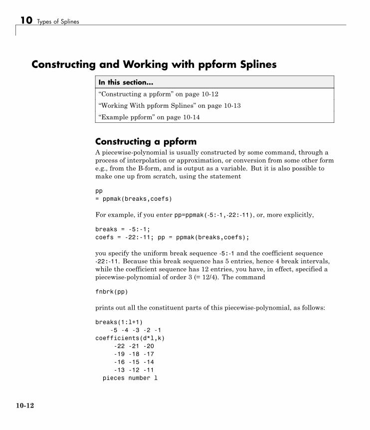
10 Types of Splines

Constructing and Working with ppform Splines

In this section...

“Constructing a ppform” on page 10-12

“Working With ppform Splines” on page 10-13

“Example ppform” on page 10-14

Constructing a ppformA piecewise-polynomial is usually constructed by some command, through aprocess of interpolation or approximation, or conversion from some other forme.g., from the B-form, and is output as a variable. But it is also possible tomake one up from scratch, using the statement

pp= ppmak(breaks,coefs)

For example, if you enter pp=ppmak(-5:-1,-22:-11), or, more explicitly,

breaks = -5:-1;coefs = -22:-11; pp = ppmak(breaks,coefs);

you specify the uniform break sequence -5:-1 and the coefficient sequence-22:-11. Because this break sequence has 5 entries, hence 4 break intervals,while the coefficient sequence has 12 entries, you have, in effect, specified apiecewise-polynomial of order 3 (= 12/4). The command

fnbrk(pp)

prints out all the constituent parts of this piecewise-polynomial, as follows:

breaks(1:l+1)-5 -4 -3 -2 -1

coefficients(d*l,k)-22 -21 -20-19 -18 -17-16 -15 -14-13 -12 -11

pieces number l

10-12


4order k

3dimension d of target

1

Further, fnbrk can be used to supply each of these parts separately. But thepoint of Curve Fitting Toolbox spline functionality is that you usually neednot concern yourself with these details. You simply use pp as an argumentto commands that evaluate, differentiate, integrate, convert, or plot thepiecewise-polynomial whose description is contained in pp.

Working With ppform SplinesHere are some functions for operations you can perform on apiecewise-polynomial.

v = fnval(pp,x) Evaluates

dpp = fnder(pp) Differentiates

dirpp = fndir(pp,dir) Differentiates in the direction dir

ipp = fnint(pp) Integrates

fnmin(pp,[a,b]) Finds the minimum value in giveninterval

fnzeros(pp,[a,b]) Finds the zeros in the given interval

pj = fnbrk(pp,j) Pulls out the jth polynomial piece

pc = fnbrk(pp,[a b]) Restricts/extends to the interval[a..b]

po = fnxtr(pp,order) Extends outside its basic interval bypolynomial of specified order

fnplt(pp,[a,b]) Plots on given interval

sp = fn2fm(pp,'B-') Converts to B-form

pr = fnrfn(pp,morebreaks) Inserts additional breaks

10-13

10 Types of Splines

Inserting additional breaks comes in handy when you want to add twopiecewise-polynomials with different breaks, as is done in the command fncmb.

Example ppformExecute the following commands to create and plot the particularpiecewise-polynomial (ppform) described in the “Constructing a ppform” onpage 10-12 section.

1 Create the piecewise-polynomial with break sequence -5:-1 and coefficientsequence -22:-11:

pp=ppmak(-5:-1,-22:-11)

2 Create the basic plot:

x = linspace(-5.5,-.5,101);plot(x, fnval(pp,x),'x')

3 Add the break lines to the plot:

breaks=fnbrk(pp,'b'); yy=axis; hold onfor j=1:fnbrk(pp,'l')+1

plot(breaks([j j]),yy(3:4))end

4 Superimpose the plot of the polynomial that supplies the third polynomialpiece:

plot(x,fnval(fnbrk(pp,3),x),'linew',1.3)set(gca,'ylim',[-60 -10]), hold off

10-14


−5.5 −5 −4.5 −4 −3.5 −3 −2.5 −2 −1.5 −1 −0.5−60

−55

−50

−45

−40

−35

−30

−25

−20

−15

−10

A Piecewise-Polynomial Function, Its Breaks, and the Polynomial GivingIts Third Piece

The figure above is the final picture. It shows the piecewise-polynomial asa sequence of points and, solidly on top of it, the polynomial from which itsthird polynomial piece is taken. It is quite noticeable that the value of apiecewise-polynomial at a break is its limit from the right, and that the valueof the piecewise-polynomial outside its basic interval is obtained by extendingits leftmost, respectively its rightmost, polynomial piece.

While the ppform of a piecewise-polynomial is efficient for evaluation, theconstruction of a piecewise-polynomial from some data is usually moreefficiently handled by determining first its B-form, i.e., its representationas a linear combination of B-splines.

10-15

10 Types of Splines

The B-form

In this section...

“Introduction to B-form” on page 10-16

“Definition of B-form” on page 10-16

“B-form and B-Splines” on page 10-17

“B-Spline Knot Multiplicity” on page 10-19

“Choice of Knots for B-form” on page 10-20

Introduction to B-formA univariate spline f is specified by its nondecreasing knot sequence t and byits B-spline coefficient sequence a. See “Multivariate Tensor Product Splines”on page 10-27 for a discussion of multivariate splines. The coefficients maybe (column-)vectors, matrices, even ND-arrays. When the coefficients are2-vectors or 3-vectors, f is a curve in R2 or R3 and the coefficients are calledthe control points for the curve.

Roughly speaking, such a spline is a piecewise-polynomial of a certainorder and with breaks t(i). But knots are different from breaks in thatthey may be repeated, i.e., t need not be strictly increasing. The resultingknot multiplicities govern the smoothness of the spline across the knots, asdetailed below.

With [d,n] = size(a), and n+k = length(t), the spline is of order k. Thismeans that its polynomial pieces have degree < k. For example, a cubicspline is a spline of order 4 because it takes four coefficients to specify a cubicpolynomial.

Definition of B-formThese four items, t, a, n, and k, make up the B-form of the spline f.

This means, explicitly, that

10-16

The B-form

f B a ii ki

n= ( )=∑ , :,

1

with Bi,k=B(·|t(i:i+k)) the ith B-spline of order k for the given knot sequencet, i.e., the B-spline with knots t(i),...,t(i+k). The basic interval of this B-formis the interval [t(1)..t(n+k)]. It is the default interval over which a spline inB-form is plotted by the command fnplt. Note that a spline in B-form is zerooutside its basic interval while, after conversion to ppform via fn2fm, this isusually not the case because, outside its basic interval, a piecewise-polynomialis defined by extension of its first or last polynomial piece. In particular, afunction in B-form may have jumps in value and/or one of its derivative notonly across its interior knots, i.e., across t(i) with t(1)<t(i)<t(n+k), but alsoacross its end knots, t(1) and t(n+k).

B-form and B-SplinesThe building blocks for the B-form of a spline are the B-splines. A B-Splineof Order 4, and the Four Cubic Polynomials from Which It Is Made on page10-18 shows a picture of such a B-spline, the one with the knot sequence [01.5 2.3 4 5], hence of order 4, together with the polynomials whose piecesmake up the B-spline. The information for that picture could be generatedby the command

bspline([0 1.5 2.3 4 5])

10-17

10 Types of Splines

A B-Spline of Order 4, and the Four Cubic Polynomials from Which It Is Made

To summarize: The B-spline with knots t(i)≤····≤ t(i+k) is positive on theinterval (t(i)..t(i+k))and is zero outside that interval. It is piecewise-polynomialof order k with breaks at the sites t(i),...,t(i+k). These knots may coincide,and the precise multiplicity governs the smoothness with which the twopolynomial pieces join there.

Definition of B-SplinesThe shorthand

f Sk t∈ ,

is one of several ways to indicate that f is a spline of order kwith knot sequencet, i.e., a linear combination of the B-splines of order k for the knot sequence t.

A word of caution: The term B-spline has been expropriated by theComputer-Aided Geometric Design (CAGD) community to mean what iscalled here a spline in B-form, with the unhappy result that, in any discussionbetween mathematicians/approximation theorists and people in CAGD, onenow always has to check in what sense the term is being used.

10-18

The B-form

B-Spline Knot MultiplicityThe rule is

knot multiplicity + condition multiplicity = order

All Third-Order B-Splines for a Certain Knot Sequence with Various KnotMultiplicities

For example, for a B-spline of order 3, a simple knot would mean twosmoothness conditions, i.e., continuity of function and first derivative, while adouble knot would only leave one smoothness condition, i.e., just continuity,and a triple knot would leave no smoothness condition, i.e., even the functionwould be discontinuous.

All Third-Order B-Splines for a Certain Knot Sequence with Various KnotMultiplicities on page 10-19 shows a picture of all the third-order B-splinesfor a certain mystery knot sequence t. The breaks are indicated by verticallines. For each break, try to determine its multiplicity in the knot sequence(it is 1,2,1,1,3), as well as its multiplicity as a knot in each of the B-splines.For example, the second break has multiplicity 2 but appears only withmultiplicity 1 in the third B-spline and not at all, i.e., with multiplicity 0, inthe last two B-splines. Note that only one of the B-splines shown has all itsknots simple. It is the only one having three different nontrivial polynomialpieces. Note also that you can tell the knot-sequence multiplicity of a knotby the number of B-splines whose nonzero part begins or ends there. The

10-19

10 Types of Splines

picture is generated by the following MATLAB statements, which use thecommand spcol from this toolbox to generate the function values of all theseB-splines at a fine net x.

t=[0,1,1,3,4,6,6,6]; x=linspace(-1,7,81);c=spcol(t,3,x);[l,m]=size(c);c=c+ones(l,1)*[0:m-1];axis([-1 7 0 m]); hold onfor tt=t, plot([tt tt],[0 m],'-'), endplot(x,c,'linew',2), hold off, axis off

Further illustrated examples are provided by the example ”Construct andWork with the B-form”. You can also use the GUI bspligui to study thedependence of a B-spline on its knots experimentally.

Choice of Knots for B-formThe rule “knot multiplicity + condition multiplicity = order” has the followingconsequence for the process of choosing a knot sequence for the B-form ofa spline approximant. Suppose the spline s is to be of order k, with basicinterval [a..b], and with interior breaks ξ2< ·· ·<ξl. Suppose, further, that, atξi, the spline is to satisfy μi smoothness conditions, i.e.,

jump D s D s D s j i li

j ji

ji i : , , ,...,= ( ) − ( ) = ≤ < =+ − 0 0 2

Then, the appropriate knot sequence t should contain the break ξi exactly k –μi times, i=2,...,l. In addition, it should contain the two endpoints, a and b, ofthe basic interval exactly k times. This last requirement can be relaxed, buthas become standard. With this choice, there is exactly one way to write eachspline s with the properties described as a weighted sum of the B-splines oforder k with knots a segment of the knot sequence t. This is the reason for theB in B-spline: B-splines are, in Schoenberg’s terminology, basic splines.

For example, if you want to generate the B-form of a cubic spline on theinterval [1 .. 3], with interior breaks 1.5, 1.8, 2.6, and with two continuousderivatives, then the following would be the appropriate knot sequence:

t = [1, 1, 1, 1, 1.5, 1.8, 2.6, 3, 3, 3, 3];

10-20

The B-form

This is supplied by augknt([1, 1.5, 1.8, 2.6, 3], 4). If you wanted,instead, to allow for a corner at 1.8, i.e., a possible jump in the first derivativethere, you would triple the knot 1.8, i.e., use

t = [1, 1, 1, 1, 1.5, 1.8, 1.8, 1.8, 2.6, 3, 3, 3, 3];

and this is provided by the statement

t = augknt([1, 1.5, 1.8, 2.6, 3], 4, [1, 3, 1] );

10-21

10 Types of Splines

Constructing and Working with B-form Splines

In this section...

“Construction of B-form” on page 10-22

“Working With B-form Splines” on page 10-23

“Example: B-form Spline Approximation to a Circle” on page 10-24

Construction of B-formUsually, a spline is constructed from some information, like function valuesand/or derivative values, or as the approximate solution of some ordinarydifferential equation. But it is also possible to make up a spline from scratch,by providing its knot sequence and its coefficient sequence to the commandspmak.

For example, if you enter

sp = spmak(1:10,3:8);

you supply the uniform knot sequence 1:10 and the coefficient sequence 3:8.Because there are 10 knots and 6 coefficients, the order must be 4(= 10 – 6),i.e., you get a cubic spline. The command

fnbrk(sp)

prints out the constituent parts of the B-form of this cubic spline, as follows:

knots(1:n+k)1 2 3 4 5 6 7 8 9 10

coefficients(d,n)3 4 5 6 7 8

number n of coefficients6

order k4

dimension d of target1

10-22


Further, fnbrk can be used to supply each of these parts separately.

But the point of the Curve Fitting Toolbox spline functionality is that thereshouldn’t be any need for you to look up these details. You simply use sp asan argument to commands that evaluate, differentiate, integrate, convert, orplot the spline whose description is contained in sp.

Working With B-form SplinesThe following commands are available for spline work. There is spmak andfnbrk to make up a spline and take it apart again. Use fn2fm to convert fromB-form to ppform. You can evaluate, differentiate, integrate, minimize, findzeros of, plot, refine, or selectively extrapolate a spline with the aid of fnval,fnder, fndir, fnint, fnmin, fnzeros, fnplt, fnrfn, and fnxtr.

There are five commands for generating knot sequences:

• augknt for providing boundary knots and also controlling the multiplicityof interior knots

• brk2knt for supplying a knot sequence with specified multiplicities

• aptknt for providing a knot sequence for a spline space of given order thatis suitable for interpolation at given data sites

• optknt for providing an optimal knot sequence for interpolation at givensites

• newknt for a knot sequence perhaps more suitable for the function to beapproximated

In addition, there is:

• aveknt to supply certain knot averages (the Greville sites) as recommendedsites for interpolation

• chbpnt to supply such sites

• knt2brk and knt2mlt for extracting the breaks and/or their multiplicitiesfrom a given knot sequence

To display a spline curve with given two-dimensional coefficient sequence anda uniform knot sequence, use spcrv.

10-23

10 Types of Splines

You can also write your own spline construction commands, in whichcase you will need to know the following. The construction of a splinesatisfying some interpolation or approximation conditions usually requires acollocation matrix, i.e., the matrix that, in each row, contains the sequenceof numbers DrBj,k(τ), i.e., the rth derivative at τ of the jth B-spline, forall j, for some r and some site τ. Such a matrix is provided by spcol. Anoptional argument allows for this matrix to be supplied by spcol in aspace-saving spline-almost-block-diagonal-form or as a MATLAB sparsematrix. It can be fed to slvblk, a command for solving linear systems withan almost-block-diagonal coefficient matrix. If you are interested in seeinghow spcol and slvblk are used in this toolbox, have a look at the commandsspapi, spap2, and spaps.

In addition, there are routines for constructing cubic splines. csapi andcsape provide the cubic spline interpolant at knots to given data, using thenot-a-knot and various other end conditions, respectively. A parametric cubicspline curve through given points is provided by cscvn. The cubic smoothingspline is constructed in csaps.

Example: B-form Spline Approximation to a CircleAs another simple example,

points = .95*[0 -1 0 1;1 0 -1 0];sp = spmak(-4:8,[points points]);

provides a planar, quartic, spline curve whose middle part is a pretty goodapproximation to a circle, as the plot on the next page shows. It is generatedby a subsequent

plot(points(1,:),points(2,:),'x'), hold onfnplt(sp,[0,4]), axis equal square, hold off

Insertion of additional control points ± ±( )0 95 0 95 1 9. , . / . would make avisually perfect circle.

Here are more details. The spline curve generated has the form Σ8j=1Bj,5a(:,j), with -4:8 the uniform knot sequence, and with its control points a(:,j) thesequence (0,α),(–α,0),(0,–α),(α,0),(0,α),(–α,0),(0,–α),(α,0) with α=0.95. Only thecurve part between the parameter values 0 and 4 is actually plotted.

10-24


To get a feeling for how close to circular this part of the curve actually is,compute its unsigned curvature. The curvature κ(t) at the curve point γ(t) =(x(t), y(t)) of a space curve γ can be computed from the formula

=−

+

x y y x

x y

’ ’’ ’ ’’

( ’ ’ ) /2 2 3 2

in which x’, x″, y’, and y” are the first and second derivatives of the curve withrespect to the parameter used (t). Treat the planar curve as a space curve inthe (x,y)-plane, hence obtain the maximum and minimum of its curvature at21 points as follows:

t = linspace(0,4,21);zt = zeros(size(t));dsp = fnder(sp); dspt = fnval(dsp,t); ddspt = fnval(fnder(dsp),t);kappa = abs(dspt(1,:).*ddspt(2,:)-dspt(2,:).*ddspt(1,:))./...

(sum(dspt.^2)).^(3/2);[min(kappa),max(kappa)]

ans =1.6747 1.8611

So, while the curvature is not quite constant, it is close to 1/radius of thecircle, as you see from the next calculation:

1/norm(fnval(sp,0))

ans =1.7864

10-25

10 Types of Splines

-1

-0.8

-0.6

-0.4

-0.2

0

0.2

0.4

0.6

0.8

1

-1 -0.5 0 0.5 1

x

x

x

x

Spline Approximation to a Circle; Control Points Are Marked x

10-26

Multivariate Tensor Product Splines


In this section...

“Introduction to Multivariate Tensor Product Splines” on page 10-27

“B-form of Tensor Product Splines” on page 10-27

“Construction With Gridded Data” on page 10-28

“ppform of Tensor Product Splines” on page 10-28

“Example: The Mobius Band” on page 10-28

Introduction to Multivariate Tensor Product SplinesThe toolbox provides (polynomial) spline functions in any number of variables,as tensor products of univariate splines. These multivariate splines come inboth standard forms, the B-form and the ppform, and their construction anduse parallels entirely that of the univariate splines discussed in previoussections, “Constructing and Working with ppform Splines” on page 10-12 and“Constructing and Working with B-form Splines” on page 10-22. The samecommands are used for their construction and use.

For simplicity, the following discussion deals just with bivariate splines.

B-form of Tensor Product SplinesThe tensor-product idea is very simple. If f is a function of x, and g is afunction of y, then their tensor-product p (x,y): = f (x)g(y) is a function of x andy, i.e., a bivariate function. More generally, with s=(s1,...,sm+h) and t=(t1,...,tn+k)knot sequences and aji:i=1,...,m;j=1,...n) a corresponding coefficient array, youobtain a bivariate spline as

f x y B x s s B y t t ai i h j j k ijj

n

i

m( , ) | ,..., | ,...,= ( ) ( )+ +

==∑∑

11

The B-form of this spline comprises the cell array {s,t} of its knot sequences,the coefficient array a, the numbers vector [m,n], and the orders vector [h,k].The command

10-27

10 Types of Splines

sp = spmak({s,t},a);

constructs this form. Further, fnplt, fnval, fnder, fndir, fnrfn, and fn2fmcan be used to plot, evaluate, differentiate and integrate, refine, and convertthis form.

Construction With Gridded DataYou are most likely to construct such a form by looking for an interpolantor approximant to gridded data. For example, if you know the valuesz(i,j)=g(x(i),y(j)),i=1:m, j=1:n, of some function g at all the points in arectangular grid, then, assuming that the strictly increasing sequence xsatisfies the Schoenberg-Whitney conditions with respect to the aboveknot sequence s, and that the strictly increasing sequence y satisfies theSchoenberg-Whitney conditions with respect to the above knot sequencet, the command

sp=spapi({s,t},[h,k],{x,y},z);

constructs the unique bivariate spline of the above form that matchesthe given values. The command fnplt(sp) gives you a quick plot of thisinterpolant. The command pp = fn2fm(sp,'pp') gives you the ppform ofthis spline, which is probably what you want when you want to evaluate thespline at a fine grid ((xx(i),yy(j)) for i=1:M, j=1:N), by the command:

values = fnval(pp,{xx,yy});

ppform of Tensor Product SplinesThe ppform of such a bivariate spline comprises, analogously, a cell array ofbreak sequences, a multidimensional coefficient array, a vector of numberpieces, and a vector of polynomial orders. Fortunately, the toolbox is set upin such a way that there is usually no reason for you to concern yourselfwith these details of either form. You use interpolation, approximation, orsmoothing to construct splines, and then use the fn... commands to makeuse of them.

Example: The Mobius BandHere is an example of a surface constructed as a 3-D-valued bivariate spline.The surface is the famous Möbius band, obtainable by taking a longish strip

10-28


of paper and gluing its narrow ends together, but with a twist. The figure isobtained by the following commands:

x = 0:1; y = 0:4; h = 1/4; o2 = 1/sqrt(2); s = 2; ss = 4;v(3,:,:) = h*[0, -1, -o2, 0, o2, 1, 0;0, 1, o2, 0, -o2, -1, 0];v(2,:,:) = [ss, 0, s-h*o2, 0, -s-h*o2, 0, ss;...

ss, 0, s+h*o2, 0,-s+h*o2, 0, ss];v(1,:,:) = s*[0, 1, 0, -1+h, 0, 1, 0; 0, 1, 0, -1-h, 0, 1, 0];cs = csape({x,y},v,{'variational','clamped'});fnplt(cs), axis([-2 2 -2.5 2.5 -.5 .5]), shading interpaxis off, hold onvalues = squeeze(fnval(cs,{1,linspace(y(1),y(end),51)}));plot3(values(1,:), values(2,:), values(3,:),'k','linew',2)view(-149,28), hold off

A Möbius Band Made by Vector-Valued Bivariate Spline Interpolation

10-29

10 Types of Splines

NURBS and Other Rational Splines

In this section...

“Introduction to Rational Splines” on page 10-30

“rsform: rpform, rBform” on page 10-30

Introduction to Rational SplinesA rational spline is, by definition, any function that is the ratio of two splines:

r x s x w x( ) = ( ) ( )/

This requires w to be scalar-valued, but s is often chosen to be vector-valued.Further, it is desirable that w(x) be not zero for any x of interest.

Rational splines are popular because, in contrast to ordinary splines, they canbe used to describe certain basic design shapes, like conic sections, exactly.

rsform: rpform, rBformThe two splines, s and w, in the rational spline r(x)=s(x)/w(x) need not berelated to one another. They could even be of different forms. But, in thecontext of this toolbox, it is convenient to restrict them to be of the sameform, and even of the same order and with the same breaks or knots. For,under that assumption, you can represent such a rational spline by the(vector-valued) spline function

R x s x w x( ) = ( ) ( )⎡⎣ ⎤⎦;

whose values are vectors with one more entry than the values of the rationalspline r, and call this the rsform of the rational spline, or, more precisely, therpform or rBform, depending on whether s and w are in ppform or in B-form.Internally, the only thing that distinguishes these rational forms from theircorresponding ordinary spline forms, rpform and B-form, is their form part,i.e., the string obtained via fnbrk(r,'form'). This is enough to alert thefn... commands to act appropriately on a function in one of the rsforms.

10-30

NURBS and Other Rational Splines

For example, as is done in fnval, it is very easy to obtain r(x) from R(x). If vis the value of R at x, then v(1:end-1)/v(end) is the value of r at x. If, inaddition, dv is DR(x), then (dv(1:end-1)-dv(end)*v(1:end-1))/v(end) isDr(x). More generally, by Leibniz’s formula,

D s D wrji

D wD rj j

i

ji j i= ( ) = ⎛

⎝⎜⎞

⎠⎟

=

−∑0

Therefore,

D r D sji

D wD r wj j i j i

i

j= −

⎛

⎝⎜⎞

⎠⎟

⎛

⎝⎜⎜

⎞

⎠⎟⎟

−

=∑

1/

This shows that you can compute the derivatives of r inductively, using thederivatives of s and w (i.e., the derivatives of R) along with the derivatives of rof order less than j to compute the jth derivative of r. This inductive schemeis used in fntlr to provide the first so many derivatives of a rational spline.There is a corresponding formula for partial and directional derivatives formultivariate rational splines.

10-31

10 Types of Splines

Constructing and Working with Rational Splines

In this section...

“Rational Spline Example: Circle” on page 10-32

“Rational Spline Example: Sphere” on page 10-33

“Functions for Working With Rational Splines” on page 10-34

Rational Spline Example: CircleFor example,

circle = rsmak('circle');

provides a rational spline whose values on its basic interval trace out the unitcircle, i.e., the circle of radius 1 with center at the origin, as the command

fnplt(circle), axis square

readily shows; the resulting output is the circle in the figure A Circle and anEllipse, Both Given by a Rational Spline on page 10-33.

It is easy to manipulate this circle to obtain related shapes. For example, thenext commands stretch the circle into an ellipse, rotate the ellipse 45 degrees,and translate it by (1,1), and then plot it on top of the circle.

ellipse = fncmb(circle,[2 0;0 1]);s45 = 1/sqrt(2);rtellipse = fncmb(fncmb(ellipse, [s45 -s45;s45 s45]), [1;1] );hold on, fnplt(rtellipse), hold off

As a further example, the "circle" just constructed is put together from fourpieces. To highlight the first such piece, use the following commands:

quarter = fnbrk(fn2fm(circle,'rp'),1);hold on, fnplt(quarter,3), hold off

In the first command, fn2fm is used to change forms, from one based on theB-form to one based on the ppform, and then fnbrk is used to extract thefirst piece, and this piece is then plotted on top of the circle in A Circle and

10-32


an Ellipse, Both Given by a Rational Spline on page 10-33, with linewidth 3to make it stand out.

−1 −0.5 0 0.5 1 1.5 2 2.5 3−1

−0.5

0

0.5

1

1.5

2

2.5

3

A Circle and an Ellipse, Both Given by a Rational Spline

Rational Spline Example: SphereAs a surface example, the command rsmak('southcap') provides a 3-vectorvalued rational bicubic polynomial whose values on the unit square [-1 .. 1]^2fill out a piece of the unit sphere. Adjoin to it five suitable rotates of it andyou get the unit sphere exactly. For illustration, the following commandsgenerate two-thirds of that sphere, as shown in Part of a Sphere Formed byFour Rotates of a Quartic Rational on page 10-34.

southcap = rsmak('southcap'); fnplt(southcap)xpcap = fncmb(southcap,[0 0 -1;0 1 0;1 0 0]);ypcap = fncmb(xpcap,[0 -1 0; 1 0 0; 0 0 1]);northcap = fncmb(southcap,-1);hold on, fnplt(xpcap), fnplt(ypcap), fnplt(northcap)axis equal, shading interp, view(-115,10), axis off, hold off

10-33

10 Types of Splines

Part of a Sphere Formed by Four Rotates of a Quartic Rational

Functions for Working With Rational SplinesHaving chosen to represent the rational spline r = s/w in this way by theordinary spline R=[s;w] makes it is easy to apply to a rational spline allthe fn... commands in the Curve Fitting Toolbox spline functions, withthe following exceptions. The integral of a rational spline need not be arational spline, hence there is no way to extend fnint to rational splines. Thederivative of a rational spline is again a rational spline but one of roughlytwice the order. For that reason, fnder and fndir will not touch rationalsplines. Instead, there is the command fntlr for computing the value ata given x of all derivatives up to a given order of a given function. If thatfunction is rational, the needed calculation is based on the considerationsgiven in the preceding paragraph.

The command r = rsmak(shape) provides rational splines in rBform thatdescribe exactly certain standard geometric shapes , like 'circle', 'arc','cylinder', 'sphere', 'cone', 'torus'. The command fncmb(r,trans)can be used to apply standard transformations to the resulting shape. Forexample, if trans is a column-vector of the right length, the shape would betranslated by that vector while, if trans is a suitable matrix like a rotation,the shape would be transformed by that matrix.

The command r = rscvn(p) constructs the quadratic rBform of atangent-continuous curve made up of circular arcs and passing through thegiven sequence, p, of points in the plane.

10-34


A special rational spline form, called a NURBS, has become a standard tool inCAGD. A NURBS is, by definition, any rational spline for which both s and ware in the same B-form, with each coefficient for s containing explicitly thecorresponding coefficient for w as a factor:

s B v i a i w B v iii

ii

= ( ) ( ) = ( )∑ ∑:, ,

The normalized coefficients a(:,i) for the numerator spline are more readilyused as control points than the unnormalized coefficients v(i)a(:,i) used in therBform. Nevertheless, this toolbox provides no special NURBS form, but onlythe more general rational spline, but in both B-form (called rBform internally)and in ppform (called rpform internally).

The rational spline circle used earlier is put together in rsmak by code likethe following.

x = [1 1 0 -1 -1 -1 0 1 1]; y = [0 1 1 1 0 -1 -1 -1 0];s45 = 1/sqrt(2); w =[1 s45 1 s45 1 s45 1 s45 1];circle = rsmak(augknt(0:4,3,2), [w.*x;w.*y;w]);

Note the appearance of the denominator spline as the last component. Alsonote how the coefficients of the denominator spline appear here explicitlyas factors of the corresponding coefficients of the numerator spline. Thenormalized coefficient sequence [x;y] is very simple; it consists of the verticesand midpoints, in proper order, of the "unit square". The resulting controlpolygon is tangent to the circle at the places where the four quadratic piecesthat form the circle abut.

For a thorough discussion of NURBS, see [G. Farin, NURBS, 2nd ed.,AKPeters Ltd, 1999] or [Les Piegl and Wayne Tiller, The NURBS Book, 2nded., Springer-Verlag, 1997].

10-35

10 Types of Splines

Constructing and Working with stform Splines

In this section...

“Introduction to the stform” on page 10-36

“Construction and Properties of the stform” on page 10-37

“Working with the stform” on page 10-38

Introduction to the stformA multivariate function form quite different from the tensor-product constructis the scattered translates form, or stform for short. As the name suggests,it uses arbitrary or scattered translates ψ(· –cj) of one fixed function ψ,in addition to some polynomial terms. Explicitly, such a form describes afunction

f x x c a p xj jj

n k( ) = −( ) + ( )

=

−

∑1

in terms of the basis function ψ, a sequence (cj) of sites called centers and acorresponding sequence (aj) of n coefficients, with the final k coefficients,an-k+1,...,an, involved in the polynomial part, p.

When the basis function is radially symmetric, meaning that ψ(x) dependsonly on the Euclidean length |x| of its argument, x, then ψ is called a radialbasis function, and, correspondingly, f is then often called an RBF.

At present, the toolbox works with just one kind of stform, namely a bivariatethin-plate spline and its first partial derivatives. For the thin-plate spline,the basis function is ψ(x) = φ(|x|2), with φ(t) = tlogt, i.e., a radial basisfunction. Its polynomial part is a linear polynomial, i.e., p(x)=x(1)an – 2+x(2)an– 1+an. The first partial derivative with respect to its first argument uses,correspondingly, the basis function ψ(x)=φ(|x|2), with φ(t) = (D1t)·(logt+1)and D1t = D1t(x) = 2x(1), and p(x) = an.

10-36

Constructing and Working with stform Splines

Construction and Properties of the stformA function in stform can be put together from its center sequence centersand its coefficient sequence coefs by the command

f = stmak(centers, coefs, type);

with the string type one of 'tp00', 'tp10', 'tp01', to indicate, respectively,a thin-plate spline, a first partial of a thin-plate spline with respect to thefirst argument, and a first partial of a thin-plate spline with respect to thesecond argument. There is one other choice, 'tp'; it denotes a thin-platespline without any polynomial part and is likely to be used only during theconstruction of a thin-plate spline, as in tpaps.

A function f in stform depends linearly on its coefficients, meaning that

f x x aj jj

n( ) = ( )

=∑

1

with ψj either a translate of the basis function Ψ or else some polynomial.Suppose you wanted to determine these coefficients aj so that the functionf matches prescribed values at prescribed sites xi. Then you would needthe collocation matrix (ψj(xi)). You can obtain this matrix by the commandstcol(centers,x,type). In fact, because the stform has aj as the jth column,coefs(:,j), of its coefficient array, it is worth noting that stcol can alsosupply the transpose of the collocation matrix. Thus, the command

values = coefs*stcol(centers,x,type,'tr');

would provide the values at the entries of x of the st function specified bycenters and type.

The stform is attractive because, in contrast to piecewise polynomial forms,its complexity is the same in any number of variables. It is quite simple,yet, because of the complete freedom in the choice of centers, very flexibleand adaptable.

On the negative side, the most attractive choices for a radial basis functionshare with the thin-plate spline that the evaluation at any site involvesall coefficients. For example, plotting a scalar-valued thin-plate spline via

10-37

10 Types of Splines

fnplt involves evaluation at a 51-by-51 grid of sites, a nontrivial task whenthere are 1000 coefficients or more. The situation is worse when you wantto determine these 1000 coefficients so as to obtain the stform of a functionthat matches function values at 1000 data sites, as this calls for solving afull linear system of order 1000, a task requiring O(10^9) flops if done by adirect method. Just the construction of the collocation matrix for this linearsystem (by stcol) takes O(10^6) flops.

The command tpaps, which constructs thin-plate spline interpolants andapproximants, uses iterative methods when there are more than 728 datapoints, but convergence of such iteration may be slow.

Working with the stformAfter you have constructed an approximating or interpolating thin-platespline st with the aid of tpaps (or directly via stmak), you can use thefollowing commands:

• fnbrk to obtain its parts or change its basic interval,

• fnval to evaluate it

• fnplt to plot it

• fnder to construct its two first partial derivatives, but no higher orderderivatives as they become infinite at the centers.

This is just one indication that the stform is quite different in nature fromthe other forms in this toolbox, hence other fn... commands by and largedon’t work with stforms. For example, it makes no sense to use fnjmp, andfnmin or fnzeros only work for univariate functions. It also makes nosense to use fnint on a function in stform because such functions cannotbe integrated in closed form.

• The command Ast = fncmb(st,A) can be used on st, provided A issomething that can be applied to the values of the function described byst. For example, A might be 'sin', in which case Ast is the stform of thefunction whose coefficients are the sine of the coefficients of st. In effect,Ast describes the function obtained by composing A with st. But, becauseof the singularities in the higher-order derivatives of a thin-plate spline,there seems little point to make fndir or fntlr applicable to such a st.

10-38

11

Advanced Spline Examples

• “Least-Squares Approximation by Natural Cubic Splines” on page 11-2

• “Solving A Nonlinear ODE” on page 11-8

• “Construction of the Chebyshev Spline” on page 11-14

• “Approximation by Tensor Product Splines” on page 11-20

11 Advanced Spline Examples

Least-Squares Approximation by Natural Cubic SplinesThe construction of a least-squares approximant usually requires that onehave in hand a basis for the space from which the data are to be approximated.As the example of the space of “natural” cubic splines illustrates, the explicitconstruction of a basis is not always straightforward.

This section makes clear that an explicit basis is not actually needed; it issufficient to have available some means of interpolating in some fashion fromthe space of approximants. For this, the fact that the Curve Fitting Toolboxspline functions support work with vector-valued functions is essential.

This section discusses these aspects of least-squares approximation by“natural” cubic splines.

• “Problem” on page 11-2

• “General Resolution” on page 11-2

• “Need for a Basis Map” on page 11-3

• “A Basis Map for “Natural” Cubic Splines” on page 11-3

• “The One-line Solution” on page 11-4

• “The Need for Proper Extrapolation” on page 11-4

• “The Correct One-Line Solution” on page 11-6

• “Least-Squares Approximation by Cubic Splines” on page 11-7

ProblemYou want to construct the least-squares approximation to given data (x,y) fromthe space S of “natural” cubic splines with given breaks b(1) < ...< b(l+1).

General ResolutionIf you know a basis, (f1,f2,...,fm), for the linear space S of all “natural” cubicsplines with break sequence b, then you have learned to find the least-squaresapproximation in the form c(1)f1+ c(2)f2+ ... + c(m)fm, with the vector cthe least-squares solution to the linear system A*c = y, whose coefficientmatrix is given by

11-2

Least-Squares Approximation by Natural Cubic Splines

A(i,j) = fj(x(i)), i=1:length(x), j=1:m .

In other words, c = A\y.

Need for a Basis MapThe general solution seems to require that you know a basis. However, inorder to construct the coefficient sequence c, you only need to know the matrixA. For this, it is sufficient to have at hand a basis map, namely a function Fsay, so that F(c) returns the spline given by the particular weighted sumc(1)f1+c(2)f2+... +c(m)fm. For, with that, you can obtain, for j=1:m, thej-th column of A as fnval(F(ej),x), with ej the j-th column of eye(m),the identity matrix of order m.

Better yet, the Curve Fitting Toolbox spline functions can handlevector-valued functions, so you should be able to construct the basis map Fto handle vector-valued coefficients c(i) as well. However, by agreement, inthis toolbox, a vector-valued coefficient is a column vector, hence the sequencec is necessarily a row vector of column vectors, i.e., a matrix. With that,F(eye(m)) is the vector-valued spline whose i-th component is the basiselement fi, i=1:m. Hence, assuming the vector x of data sites to be a rowvector, fnval(F(eye(m)),x) is the matrix whose (i,j)-entry is the value offi at x(j), i.e., the transpose of the matrix A you are seeking. On the otherhand, as just pointed out, your basis map F expects the coefficient sequencec to be a row vector, i.e., the transpose of the vector A\y. Hence, assuming,correspondingly, the vector y of data values to be a row vector, you can obtainthe least-squares approximation from S to data (x,y) as

F(y/fnval(F(eye(m)),x))

To be sure, if you wanted to be prepared for x and y to be arbitrary vectors (ofthe same length), you would use instead

F(y(:).'/fnval(F(eye(m)),x(:).'))

A Basis Map for “Natural” Cubic SplinesWhat exactly is required of a basis map F for the linear space S of “natural”cubic splines with break sequence b(1) < ... < b(l+1)? Assuming thedimension of this linear space is m, the map F should set up a linear one-to-one

11-3


correspondence between m-vectors and elements of S. But that is exactly whatcsape(b, . ,'var') does.

To be explicit, consider the following function F:

function s = F(c)s = csape(b,c,'var');

For given vector c (of the same length as b), it provides the unique “natural”cubic spline with break sequence b that takes the value c(i) at b(i),i=1:l+1. The uniqueness is key. It ensures that the correspondence betweenthe vector c and the resulting spline F(c) is one-to-one. In particular, m equalslength(b). More than that, because the value f(t) of a function f at a pointt depends linearly on f, this uniqueness ensures that F(c) depends linearlyon c (because c equals fnval(F(c),b) and the inverse of an invertible linearmap is again a linear map).

The One-line SolutionPutting it all together, you arrive at the following code

csape(b,y(:).'/fnval(csape(b,eye(length(b)),'var'),x(:).'),...'var')

for the least-squares approximation by “natural” cubic splines with breaksequence b.

The Need for Proper ExtrapolationLet’s try it on some data, the census data, say, which is provided in MATLABby the command

load census

and which supplies the years, 1790:10:1990, as cdate and the values as pop.Use the break sequence 1810:40:1970.

b = 1810:40:1970;s = csape(b, ...pop(:)'/fnval(csape(b,eye(length(b)),'var'),cdate(:)'),'var');fnplt(s, [1750,2050],2.2);

11-4


hold onplot(cdate,pop,'or');hold off

Have a look at Least-Squares Approximation by “Natural” Cubic Splines WithThree Interior Breaks on page 11-6 which shows, in thick blue, the resultingapproximation, along with the given data.

This looks like a good approximation, -- except that it doesn’t look like a“natural” cubic spline. A “natural” cubic spline, to recall, must be linear to theleft of its first break and to the right of its last break, and this approximationsatisfies neither condition. This is due to the following facts.

The “natural” cubic spline interpolant to given data is provided by csapein ppform, with the interval spanned by the data sites its basic interval.On the other hand, evaluation of a ppform outside its basic interval isdone, in MATLAB ppval or Curve Fitting Toolbox spline function fnval,by using the relevant polynomial end piece of the ppform, i.e., by full-orderextrapolation. In case of a “natural” cubic spline, you want insteadsecond-order extrapolation. This means that you want, to the left of the firstbreak, the straight line that agrees with the cubic spline in value and slopeat the first break. Such an extrapolation is provided by fnxtr. Because the“natural” cubic spline has zero second derivative at its first break, such anextrapolation is even third-order, i.e., it satisfies three matching conditions.In the same way, beyond the last break of the cubic spline, you want thestraight line that agrees with the spline in value and slope at the last break,and this, too, is supplied by fnxtr.

11-5


1750 1800 1850 1900 1950 2000 2050−50

0

50

100

150

200

250

300

350

400

incorrect approximationpopulationcorrect approximation

Least-Squares Approximation by “Natural” Cubic Splines With Three InteriorBreaks

The Correct One-Line SolutionThe following one-line code provides the correct least-squares approximationto data (x,y) by “natural” cubic splines with break sequence b:

fnxtr(csape(b,y(:).'/ ...fnval(fnxtr(csape(b,eye(length(b)),'var')),x(:).'),'var'))

But it is, admittedly, a rather long line.

The following code uses this correct formula and plots, in a thinner, redline, the resulting approximation on top of the earlier plots, as shown inLeast-Squares Approximation by “Natural” Cubic Splines With Three InteriorBreaks on page 11-6.

ss = fnxtr(csape(b,pop(:)'/ ...fnval(fnxtr(csape(b,eye(length(b)),'var')),cdate(:)'),'var'));

hold on, fnplt(ss,[1750,2050],1.2,'r'),grid, hold offlegend('incorrect approximation','population', ...'correct approximation')

11-6


Least-Squares Approximation by Cubic SplinesThe one-line solution works perfectly if you want to approximate by the spaceS of all cubic splines with the given break sequence b. You don’t even have touse the Curve Fitting Toolbox spline functions for this because you can relyon the MATLAB spline. You know that, with c a sequence containing twomore entries than does b, spline(b,c) provides the unique cubic spline withbreak sequence b that takes the value c(i+1) at b(i), all i, and takes theslope c(1) at b(1), and the slope c(end) at b(end). Hence, spline(b,.)is a basis map for S.

More than that, you know that spline(b,c,xi) provides the value(s) atxi of this interpolating spline. Finally, you know that spline can handlevector-valued data. Therefore, the following one-line code constructs theleast-squares approximation by cubic splines with break sequence b to data(x,y) :

spline(b,y(:)'/spline(b,eye(length(b)),x(:)'))

11-7


Solving A Nonlinear ODEThis section discusses these aspects of a nonlinear ODE problem:

• “Problem” on page 11-8

• “Approximation Space” on page 11-8

• “Discretization” on page 11-9

• “Numerical Problem” on page 11-9

• “Linearization” on page 11-10

• “Linear System to Be Solved” on page 11-10

• “Iteration” on page 11-11

You can run this example: “Solving a Nonlinear ODE with a Boundary Layerby Collocation”.

ProblemConsider the nonlinear singularly perturbed problem:

D g x g x on2 21 0 1( ) + ( )( ) = [ ]..

Dg g0 1 0( ) = ( ) =

Approximation SpaceSeek an approximate solution by collocation from C1 piecewise cubics with asuitable break sequence; for instance,

breaks = (0:4)/4;

Because cubics are of order 4, you have

k = 4;

Obtain the corresponding knot sequence as

11-8

Solving A Nonlinear ODE

knots = augknt(breaks,k,2);

This gives a quadruple knot at both 0 and 1, which is consistent with the factthat you have cubics, i.e., have order 4.

This implies that you have

n = length(knots)-k;n = 10;

i.e., 10 degrees of freedom.

DiscretizationYou collocate at two sites per polynomial piece, i.e., at eight sites altogether.This, together with the two side conditions, gives us 10 conditions, whichmatches the 10 degrees of freedom.

Choose the two Gaussian sites for each interval. For the standard interval[–0.5,0.5] of length 1, these are the two sites

gauss = .5773502692*[-1/2; 1/2];

From this, you obtain the whole collection of collocation sites by

ninterv = length(breaks)-1;temp = ((breaks(2:ninterv+1)+breaks(1:ninterv))/2);temp = temp([1 1],:) + gauss*diff(breaks);colsites = temp(:).';

Numerical ProblemWith this, the numerical problem you want to solve is to find y S knots∈ 4,that satisfies the nonlinear system

Dy

y x D y x xy

( )

( ( )) ( )( )

0 0

11 0

2 2

=

+ = ∈=

for colsites

11-9


LinearizationIf y is your current approximation to the solution, then the linear problem forthe supposedly better solution z by Newton’s method reads

Dz

w x z x D z x b x x

z

( )

( ) ( ) ( ) ( )

0 0

02

=

+ = ∈ for colsites(1)=0

with w0(x)=2y(x),b(x)=(y(x))2+1. In fact, by choosing

w w

w x w x x0 1

1 2

1 1 0 10

( ) : , ( ) :( ) : , ( ) := == = ∈

for colsites

and choosing all other values of w0,w1,w2, b not yet specified to be zero, youcan give your system the uniform shape

w x z x w x Dz x w x D z x b x x0 1 22( ) ( ) + ( ) ( ) + ( ) ( ) = ( ) ∈, for sites

with

sites = [0,colsites,1];

Linear System to Be SolvedBecause z S4,knots, convert this last system into a system for the B-splinecoefficients of z. This requires the values, first, and second derivatives atevery x sites and for all the relevant B-splines. The command spcol wasexpressly written for this purpose.

Use spcol to supply the matrix

colmat = ...spcol(knots,k,brk2knt(sites,3));

From this, you get the collocation matrix by combining the row triple of colmatfor x using the weights w0(x),w1(x),w2(x) to get the row for x of the actualmatrix. For this, you need a current approximation y. Initially, you get it byinterpolating some reasonable initial guess from your piecewise-polynomial

11-10


space at the sites. Use the parabola x2–1, which satisfies the end conditionsas the initial guess, and pick the matrix from the full matrix colmat. Here itis, in several cautious steps:

intmat = colmat([2 1+(1:(n-2))*3,1+(n-1)*3],:);coefs = intmat\[0 colsites.*colsites-1 0].';y = spmak(knots,coefs.');

Plot the initial guess, and turn hold on for subsequent plotting:

fnplt(y,'g');legend('Initial Guess (x^2-1)','location','NW');axis([-0.01 1.01 -1.01 0.01]);hold on

IterationYou can now complete the construction and solution of the linear system forthe improved approximate solution z from your current guess y. In fact, withthe initial guess y available, you now set up an iteration, to be terminatedwhen the change z–y is small enough. Choose a relatively mild ε = .1.

tolerance = 6.e-9;epsilon = .1;while 1

vtau = fnval(y,colsites);weights=[0 1 0;

[2*vtau.' zeros(n-2,1) repmat(epsilon,n-2,1)];1 0 0];

colloc = zeros(n,n);for j=1:n

colloc(j,:) = weights(j,:)*colmat(3*(j-1)+(1:3),:);endcoefs = colloc\[0 vtau.*vtau+1 0].';z = spmak(knots,coefs.');fnplt(z,'k');maxdif = max(max(abs(z.coefs-y.coefs)));fprintf('maxdif = %g\n',maxdif)if (maxdif<tolerance), break, end

% now reiteratey = z;

11-11


endlegend({'Initial Guess (x^2-1)' 'Iterates'},'location','NW');

The resulting printout of the errors is:

maxdif = 0.206695maxdif = 0.01207maxdif = 3.95151e-005maxdif = 4.43216e-010

If you now decrease ε, you create more of a boundary layer near the rightendpoint, and this calls for a nonuniform mesh.

Use newknt to construct an appropriate finer mesh from the currentapproximation:

knots = newknt(z, ninterv+1); breaks = knt2brk(knots);knots = augknt(breaks,4,2);n = length(knots)-k;

From the new break sequence, you generate the new collocation site sequence:

ninterv = length(breaks)-1;temp = ((breaks(2:ninterv+1)+breaks(1:ninterv))/2);temp = temp([1 1], :) + gauss*diff(breaks);colpnts = temp(:).';sites = [0,colpnts,1];

Use spcol to supply the matrix

colmat = spcol(knots,k,sort([sites sites sites]));

and use your current approximate solution z as the initial guess:

intmat = colmat([2 1+(1:(n-2))*3,1+(n-1)*3],:);y = spmak(knots,[0 fnval(z,colpnts) 0]/intmat.');

Thus set up, divide ε by 3 and repeat the earlier calculation, starting withthe statements

tolerance=1.e-9;while 1

11-12


vtau=fnval(y,colpnts);...

Repeated passes through this process generate a sequence of solutions, for ε =1/10, 1/30, 1/90, 1/270, 1/810. The resulting solutions, ever flatter at 0 andever steeper at 1, are shown in the example plot. The plot also shows the finalbreak sequence, as a sequence of vertical bars. To view the plots, run theexample “Solving a Nonlinear ODE with a Boundary Layer by Collocation”.

In this example, at least, newknt has performed satisfactorily.

11-13


Construction of the Chebyshev SplineThis section discusses these aspects of the Chebyshev spline construction:

• “What Is a Chebyshev Spline?” on page 11-14

• “Choice of Spline Space” on page 11-14

• “Initial Guess” on page 11-15

• “Remez Iteration” on page 11-16

What Is a Chebyshev Spline?The Chebyshev spline C=Ct=Ck,t of order k for the knot sequence t=(ti: i=1:n+k)is the unique element of Sk,t of max-norm 1 that maximally oscillates onthe interval [tk..tn+1] and is positive near tn+1. This means that there is aunique strictly increasing n-sequence τ so that the function C=Ct Sk,t given byC(τi)=(–1)

n – 1, all i, has max-norm 1 on [tk..tn+1]. This implies that τ1=tk,τn=tn+1,and that ti < τi < tk+i, for all i. In fact, ti+1 ≤ τi ≤ ti+k–1, all i. This brings up thepoint that the knot sequence is assumed to make such an inequality possible,i.e., the elements of Sk,t are assumed to be continuous.

In short, the Chebyshev spline C looks just like the Chebyshev polynomial. Itperforms similar functions. For example, its extreme sites τ are particularlygood sites to interpolate at from Sk,t because the norm of the resultingprojector is about as small as can be; see the toolbox command chbpnt.

You can run the example Construction of a Chebyshev Spline to constructC for a particular knot sequence t.

Choice of Spline SpaceYou deal with cubic splines, i.e., with order

k = 4;

and use the break sequence

breaks = [0 1 1.1 3 5 5.5 7 7.1 7.2 8];lp1 = length(breaks);

11-14

Construction of the Chebyshev Spline

and use simple interior knots, i.e., use the knot sequence

t = breaks([ones(1,k) 2:(lp1-1) lp1(:,ones(1,k))]);n = length(t)-k;

Note the quadruple knot at each end. Because k = 4, this makes [0..8]= [breaks(1)..breaks(lp1)] the interval [tk..tn+1] of interest, with n =length(t)-k the dimension of the resulting spline space Sk,t. The same knotsequence would have been supplied by

t=augknt(breaks,k);

Initial GuessAs the initial guess for the τ, use the knot averages

t t t ki i i k= + + −+ + −( ... ) /( )1 1 1

recommended as good interpolation site choices. These are supplied by

tau=aveknt(t,k);

Plot the resulting first approximation to C, i.e., the spline c that satisfiesc(τi)=(–1)

n-–i, all i:

b = cumprod(repmat(-1,1,n)); b = b*b(end);c = spapi(t,tau,b);fnplt(c,'-.')grid

Here is the resulting plot.

11-15


-2

-1.5

-1

-0.5

0

0.5

1

1.5

0 1 2 3 4 5 6 7 8-2

-1.5

-1

-0.5

0

0.5

1

1.5

0 1 2 3 4 5 6 7 8

First Approximation to a Chebyshev Spline

Remez IterationStarting from this approximation, you use the Remez algorithm to producea sequence of splines converging to C. This means that you construct new τas the extrema of your current approximation c to C and try again. Hereis the entire loop.

You find the new interior τi as the zeros of Dc, i.e., the first derivative of c,in several steps. First, differentiate:

Dc = fnder(c);

Next, take the zeros of the control polygon of Dc as your first guess for thezeros of Dc. For this, you must take apart the spline Dc.

[knots,coefs,np,kp] = fnbrk(Dc,'knots','coefs','n','order');

11-16


The control polygon has the vertices (tstar(i),coefs(i)), with tstar theknot averages for the spline, provided by aveknt:

tstar = aveknt(knots,kp);

Here are the zeros of the resulting control polygon of Dc:

npp = (1:np-1);guess = tstar(npp) -coefs(npp).*(diff(tstar)./diff(coefs));

This provides already a very good first guess for the actual zeros.

Refine this estimate for the zeros of Dc by two steps of the secant method,taking tau and the resulting guess as your first approximations. First,evaluate Dc at both sets:

sites = tau(ones(4,1),2:n-1);sites(1,:) = guess;values = zeros(4,n-2);values(1:2,:) = reshape(fnval(Dc,sites(1:2,:)),2,n-2);

Now come two steps of the secant method. You guard against division by zeroby setting the function value difference to 1 in case it is zero. Because Dc isstrictly monotone near the sites sought, this is harmless:

for j=2:3rows = [j,j-1];Dcd=diff(values(rows,:));Dcd(find(Dcd==0)) = 1;sites(j+1,:) = sites(j,:) ...

-values(j,:).*(diff(sites(rows,:))./Dcd);values(j+1,:) = fnval(Dc,sites(j+1,:));

end

The check

max(abs(values.'))ans = 4.1176 5.7789 0.4644 0.1178

shows the improvement.

Now take these sites as your new tau,

11-17


tau = [tau(1) sites(4,:) tau(n)];

and check the extrema values of your current approximation there:

extremes = abs(fnval(c, tau));

The difference

max(extremes)-min(extremes)ans = 0.6905

is an estimate of how far you are from total leveling.

Construct a new spline corresponding to the new choice of tau and plot iton top of the old:

c = spapi(t,tau,b);sites = sort([tau (0:100)*(t(n+1)-t(k))/100]);values = fnval(c,sites);hold on, plot(sites,values)

The following code turns on the grid and plots the locations of the extrema.

grid onplot( tau(2:end-1), zeros( 1, np-1 ), 'o' )hold offlegend( 'Initial Guess', 'Current Guess', 'Extreme Locations',...'location', 'NorthEastOutside' );

Following is the resulting figure (legend not shown).

11-18


-2

-1.5

-1

-0.5

0

0.5

1

1.5

0 1 2 3 4 5 6 7 8-2

-1.5

-1

-0.5

0

0.5

1

1.5

0 1 2 3 4 5 6 7 8

o o o o o o o o o o

A More Nearly Level Spline

If this is not close enough, one simply reiterates the loop. For this example,the next iteration already produces C to graphic accuracy.

11-19


Approximation by Tensor Product SplinesBecause the toolbox can handle splines with vector coefficients, it is easy toimplement interpolation or approximation to gridded data by tensor productsplines, as the following illustration is meant to show. You can also run theexample “Bivariate Tensor Product Splines”.

To be sure, most tensor product spline approximation to gridded data can beobtained directly with one of the spline construction commands, like spapior csape, in this toolbox, without concern for the details discussed in thisexample. Rather, this example is meant to illustrate the theory behind thetensor product construction, and this will be of help in situations not coveredby the construction commands in this toolbox.

This section discusses these aspects of the tensor product spline problem:

• “Choice of Sites and Knots” on page 11-20

• “Least Squares Approximation as Function of y” on page 11-21

• “Approximation to Coefficients as Functions of x” on page 11-22

• “The Bivariate Approximation” on page 11-27

• “Switch in Order” on page 11-25

• “Approximation to Coefficients as Functions of y” on page 11-26

• “The Bivariate Approximation” on page 11-27

• “Comparison and Extension” on page 11-28

Choice of Sites and KnotsConsider, for example, least squares approximation to given dataz(i,j)=f(x(i),y(j)),i=1:Nx,j=1:Ny. You take the data from a function usedextensively by Franke for the testing of schemes for surface fitting (see R.Franke, “A critical comparison of some methods for interpolation of scattereddata,” Naval Postgraduate School Techn. Rep. NPS-53-79-003, March 1979).Its domain is the unit square. You choose a few more data sites in thex-direction than the y-direction; also, for a better definition, you use higherdata density near the boundary.

x = sort([(0:10)/10,.03 .07, .93 .97]);

11-20

Approximation by Tensor Product Splines

y = sort([(0:6)/6,.03 .07, .93 .97]);[xx,yy] = ndgrid(x,y); z = franke(xx,yy);

Least Squares Approximation as Function of yTreat these data as coming from a vector-valued function, namely, thefunction of y whose value at y(j) is the vector z(:,j), all j. For no particularreason, choose to approximate this function by a vector-valued parabolicspline, with three uniformly spaced interior knots. This means that youchoose the spline order and the knot sequence for this vector-valued spline as

ky = 3; knotsy = augknt([0,.25,.5,.75,1],ky);

and then use spap2 to provide the least squares approximant to the data:

sp = spap2(knotsy,ky,y,z);

In effect, you are finding simultaneously the discrete least squaresapproximation from Sky,knotsy to each of the Nx data sets

y j z i j i NxjNy( ) ( )( ) ==

, , , :1

1

In particular, the statements

yy = -.1:.05:1.1;vals = fnval(sp,yy);

provide the array vals, whose entry vals(i,j) can be taken as anapproximation to the value f(x(i),yy(j))of the underlying function f atthe mesh-point x(i),yy(j) because vals(:,j) is the value at yy(j) of theapproximating spline curve in sp.

This is evident in the following figure, obtained by the command:

mesh(x,yy,vals.'), view(150,50)

Note the use of vals.', in the mesh command, needed because of the MATLABmatrix-oriented view when plotting an array. This can be a serious problemin bivariate approximation because there it is customary to think of z(i, j) as

11-21


the function value at the point (x(i), y(j)), while MATLAB thinks of z(i, j) asthe function value at the point (x(j), y(i)).

0

0.2

0.4

0.6

0.8

1

−0.2

0

0.2

0.4

0.6

0.8

1

1.2

0

0.5

1

1.5

A Family of Smooth Curves Pretending to Be a Surface

Note that both the first two and the last two values on each smooth curve areactually zero because both the first two and the last two sites in yy are outsidethe basic interval for the spline in sp.

Note also the ridges. They confirm that you are plotting smooth curves inone direction only.

Approximation to Coefficients as Functions of xTo get an actual surface, you now have to go a step further. Look at thecoefficients coefsy of the spline in sp:

coefsy = fnbrk(sp,'coefs');

11-22


Abstractly, you can think of the spline in sp as the function

y coefsy r B yr kyr

| :, ,→ ( ) ( )∑

with the ith entry coefsy(i,r) of the vector coefficient coefsy(:,r)corresponding to x(i), for all i. This suggests approximating each coefficientvector coefsy(q,:) by a spline of the same order kx and with the sameappropriate knot sequence knotsx. For no particular reason, this time usecubic splines with four uniformly spaced interior knots:

kx = 4; knotsx = augknt([0:.2:1],kx);sp2 = spap2(knotsx,kx,x,coefsy.');

Note that spap2(knots,k,x,fx) expects fx(:,j) to be the datum at x(j), i.e.,expects each column of fx to be a function value. To fit the datum coefsy(q,:) at x(q), for all q, present spap2 with the transpose of coefsy.

The Bivariate ApproximationNow consider the transpose of the coefficients cxy of the resulting spline curve:

coefs = fnbrk(sp2,'coefs').';

It provides the bivariate spline approximation

x y coefs q r B x B yq kx r kyrq

, | , , ,( ) → ( ) ( ) ( )∑∑

to the original data

x i y j z x i y j i Nx j Ny( ) ( )( ) → ( ) ( )( ) = =, | , , : , :1 1

To plot this spline surface over a grid, e.g., the grid

xv = 0:.025:1; yv = 0:.025:1;

you can do the following:

11-23


values = spcol(knotsx,kx,xv)*coefs*spcol(knotsy,ky,yv).';mesh(xv,yv,values.'), view(150,50);

This results in the following figure.

0

0.2

0.4

0.6

0.8

1

00.1

0.20.3

0.40.5

0.60.7

0.80.9

1

0

0.5

1

1.5

Spline Approximation to Franke’s Function

This makes good sense because spcol(knotsx,kx,xv) is the matrix whose(i,q)th entry equals the value Bq,kx(xv(i)) at xv(i) of the qth B-spline of order kxfor the knot sequence knotsx.

Because the matrices spcol(knotsx,kx,xv) and spcol(knotsy,ky,yv) arebanded, it may be more efficient, though perhaps more memory-consuming,for large xv and yv to make use of fnval, as follows:

value2 = ...fnval(spmak(knotsx,fnval(spmak(knotsy,coefs),yv).'),xv).';

This is, in fact, what happens internally when fnval is called directly with atensor product spline, as in

value2 = fnval(spmak({knotsx,knotsy},coefs),{xv,yv});

Here is the calculation of the relative error, i.e., the difference between thegiven data and the value of the approximation at those data sites as comparedwith the magnitude of the given data:

11-24


errors = z - spcol(knotsx,kx,x)*coefs*spcol(knotsy,ky,y).';disp( max(max(abs(errors)))/max(max(abs(z))) )

The output is 0.0539, perhaps not too impressive. However, the coefficientarray was only of size 8 6

disp(size(coefs))

to fit a data array of size 15 11.

disp(size(z))

Switch in OrderThe approach followed here seems biased, in the following way. First think ofthe given data z as describing a vector-valued function of y, and then treatthe matrix formed by the vector coefficients of the approximating curve asdescribing a vector-valued function of x.

What happens when you take things in the opposite order, i.e., think of zas describing a vector-valued function of x, and then treat the matrix madeup from the vector coefficients of the approximating curve as describing avector-valued function of y?

Perhaps surprisingly, the final approximation is the same, up to roundoff.Here is the numerical experiment.

Least Squares Approximation as Function of xFirst, fit a spline curve to the data, but this time with x as the independentvariable, hence it is the rows of z that now become the data values.Correspondingly, you must supply z.', rather than z, to spap2,

spb = spap2(knotsx,kx,x,z.');

thus obtaining a spline approximation to all the curves (x ; z (:, j)). Inparticular, the statement

valsb = fnval(spb,xv).';

11-25


provides the matrix valsb, whose entry valsb(i, j) can be taken as anapproximation to the value f(xv(i),y(j)) of the underlying function f at themesh-point (xv(i),y(j)). This is evident when you plot valsb using mesh:

mesh(xv,y,valsb.'), view(150,50)

00.2

0.40.6

0.81

0

0.2

0.4

0.6

0.8

1

0

0.5

1

1.5

Another Family of Smooth Curves Pretending to Be a Surface

Note the ridges. They confirm that you are, once again, plotting smooth curvesin one direction only. But this time the curves run in the other direction.

Approximation to Coefficients as Functions of yNow comes the second step, to get the actual surface. First, extract thecoefficients:

coefsx = fnbrk(spb,'coefs');

Then fit each coefficient vector coefsx(r,:) by a spline of the same order kyand with the same appropriate knot sequence knotsy:

spb2 = spap2(knotsy,ky,y,coefsx.');

Note that, once again, you need to transpose the coefficient array from spb,because spap2 takes the columns of its last input argument as the data values.

11-26


Correspondingly, there is now no need to transpose the coefficient arraycoefsb of the resulting curve:

coefsb = fnbrk(spb2,'coefs');

The Bivariate ApproximationThe claim is that coefsb equals the earlier coefficient array coefs, up toround-off, and here is the test:

disp( max(max(abs(coefs - coefsb))) )

The output is 1.4433e-15.

The explanation is simple enough: The coefficients c of the spline s containedin sp = spap2(knots,k,x,y) depend linearly on the input values y. Thisimplies, given that both c and y are 1-row matrices, that there is some matrixA=Aknots,k,x so that

c yA k x= knots, ,

for any data y. This statement even holds when y is a matrix, of size d-by-N,say, in which case each datum y(:,j) is taken to be a point in Rd, and theresulting spline is correspondingly d-vector-valued, hence its coefficient arrayc is of size d-by-n, with n = length(knots)-k.

In particular, the statements

sp = spap2(knotsy,ky,y,z);coefsy =fnbrk(sp,'coefs');

provide us with the matrix coefsy that satisfies

coefs knotsy,ky,yy z A= .

The subsequent computations

sp2 = spap2(knotsx,kx,x,coefsy.');coefs = fnbrk(sp2,'coefs').';

11-27


generate the coefficient array coefs, which, taking into account the twotranspositions, satisfies

coefs knotsy,ky,y knotsx,kx,x

knotsx,kx,x

= ( )( )= ( )

zA A

A z A

’. ’

’. . kknotsy,ky,y

In the second, alternative, calculation, you first computed

spb = spap2(knotsx,kx,x,z.');coefsx = fnbrk(spb,'coefs');

hence coefsx=z’.Aknotsx,kx,x. The subsequent calculation

spb2 = spap2(knotsy,ky,y,coefsx.');coefsb = fnbrk(spb,'coefs');

then provided

coefsb coefsx knotsy,ky,y knotsx,kx,x knotsy,ky= = ( ).’. .’. .A A z A ,,y

Consequently, coefsb = coefs.

Comparison and ExtensionThe second approach is more symmetric than the first in that transpositiontakes place in each call to spap2 and nowhere else. This approach can be usedfor approximation to gridded data in any number of variables.

If, for example, the given data over a three-dimensional grid are contained insome three-dimensional array v of size [Nx,Ny,Nz], with v(i,j,k) containingthe value f(x(i),y(j),z(k)), then you would start off with

coefs = reshape(v,Nx,Ny*Nz);

Assuming that nj = knotsj - kj, for j = x,y,z, you would then proceed asfollows:

sp = spap2(knotsx,kx,x,coefs.');

11-28


coefs = reshape(fnbrk(sp,'coefs'),Ny,Nz*nx);sp = spap2(knotsy,ky,y,coefs.');coefs = reshape(fnbrk(sp,'coefs'),Nz,nx*ny);sp = spap2(knotsz,kz,z,coefs.');coefs = reshape(fnbrk(sp,'coefs'),nx,ny*nz);

See Chapter 17 of PGS or [C. de Boor, “Efficient computer manipulationof tensor products,” ACM Trans. Math. Software 5 (1979), 173–182;Corrigenda, 525] for more details. The same references also make clearthat there is nothing special here about using least squares approximation.Any approximation process, including spline interpolation, whose resultingapproximation has coefficients that depend linearly on the given data, canbe extended in the same way to a multivariate approximation process togridded data.

This is exactly what is used in the spline construction commands csapi,csape, spapi, spaps, and spap2, when gridded data are to be fitted. It is alsoused in fnval, when a tensor product spline is to be evaluated on a grid.

11-29


11-30

A

Splines Glossary

A Splines Glossary

List of Terms for Spline FittingThis glossary provides brief definitions of the basic mathematical terms andnotation used in this guide to splines. The terms are not in alphabetical order.Terms and definitions are presented in order such that the explanation ofeach term only uses terms discussed earlier.

In this way, you may, the first time around, choose to read the entire glossaryfrom start to finish, for a cohesive introduction to these terms.

IntervalsBecause MATLAB uses the notation [a,b] to indicate a matrix with thetwo columns, a and b, this guide uses the notation [a .. b] to indicate theclosed interval with endpoints a and b. This guide does the same foropen and half-open intervals. For example, [a .. b) denotes the intervalthat includes its left endpoint, a, and excludes its right endpoint, b.

VectorsA d-vector is a list of d real numbers, i.e., a point in ℜd. In MATLAB,a d-vector is stored as a matrix of size [1,d], i.e., as a row-vector, oras a matrix of size [d,1], i.e., as a column-vector. In the Curve FittingToolbox spline functions, vectors are column vectors.

FunctionsIn this toolbox, the term function is used in its mathematical sense,and so describes any rule that associates, to each element of a certainset called its domain, some element in a certain set called its target.Common examples in this toolbox are polynomials and splines. Buteven a point x in ℜd, i.e., a d-vector, may be thought of as a function,namely the function, with domain the set {1,...,d} and target the realnumbers ℜ, that, for i = 1,...,d, associates to i the real number x(i).

The range of a function is the set of its values.

There are scalar-valued, vector-valued, matrix-valued, and ND-valuedsplines. Scalar-valued functions have the real numbers ℜ (or, moregenerally, the complex numbers) as their target, while d-vector-valuedfunctions have ℜd as their target; if, more generally, d is a vector ofpositive integers, then d-valued functions have the d-dimensional realarrays as their target. Curve Fitting Toolbox spline functions can deal

A-2

List of Terms for Spline Fitting

with univariate and multivariate functions. The former have some realinterval, or, perhaps, all of ℜ as their domain, while m-variate functionshave some subset, or perhaps all, of ℜm as their domain.

Placeholder notationIf f is a bivariate function, and y is some specific value of its secondvariable, then

f y⋅( ),

is the univariate function whose value at x is f(x,y).

Curves and surfaces vs. functionsIn this toolbox, the term function usually refers to a scalar-valuedfunction. A vector-valued function is called here a:

curve if its domain is some interval

surface if its domain is some rectangle

To be sure, to a mathematician, a curve is not a vector-valued functionon some interval but, rather, the range of such a (continuous) function,with the function itself being just one of infinitely many possibleparametrizations of that curve.

Tensor productsA bivariate tensor product is any weighted sum of products of a functionin the first variable with a function in the second variable, i.e., anyfunction of the form

f x y a i j g x h yi jji

( , ) ( , ) ( ) ( ).= ∑∑More generally, an m-variate tensor product is any weighted sum ofproducts g1(x1)g2(x2)...gm(xm) of m univariate functions.

PolynomialsA univariate scalar-valued polynomial is specified by the list of itspolynomial coefficients. The length of that list is the order of thatpolynomial, and, in this toolbox, the list is always stored as a row vector.Hence an m-list of polynomials of order k is always stored as a matrixof size [m,k].

A-3

A Splines Glossary

The coefficients in a list of polynomial coefficients are listed from"highest" to "lowest", to conform to the MATLAB convention, as in thecommand polyval(a,x). To recall: assuming that x is a scalar and thata has k entries, this command returns the number

a x a x a k x a kk k( ) ( ) ( ) ( ).1 2 11 2− −+ + + − +

In other words, the command treats the list a as the coefficients in apower form. For reasons of numerical stability, such a coefficient list istreated in this toolbox, more generally, as the coefficients in a shifted,or, local power form, for some given center c. This means that thevalue of the polynomial at some point x is supplied by the commandpolyval(a,x-c).

A vector-valued polynomial is treated in exactly the same way, exceptthat now each polynomial coefficient is a vector, say a d-vector.Correspondingly, the coefficient list now becomes a matrix of size [d,k].

Multivariate polynomials appear in this toolbox mainly as tensorproducts. Assuming first, for simplicity, that the polynomial in questionis scalar-valued but m-variate, this means that its coefficient “list” a isan m-dimensional array, of size [k1,...,km] say, and its value at somem-vector x is, correspondingly, given by

i

k

mk i

m mk i

a i i x i c i x i c i m m

1

11 1

11 1 1

=

− −∑ ( ) − ( )( ) ( ) − ( )( )( ,..., ) ,ii

k

m

m

=∑

1

for some "center" c.

Piecewise-polynomialsA piecewise-polynomial function refers to a function put together frompolynomial pieces. If the function is univariate, then, for some strictlyincreasing sequence ξ1 < ... < ξl + 1, and for i = 1:l, it agrees with somepolynomial pi on the interval [ξi .. ξi + 1). Outside the interval [ξ1 .. ξl + 1),its value is given by its first, respectively its last, polynomial piece. Theξi are its breaks. All the multivariate piecewise-polynomials in thistoolbox are tensor products of univariate ones.

B-splinesIn this toolbox, the term B-spline is used in its original meaning only,as given to it by its creator, I. J. Schoenberg, and further amplified in

A-4


his basic 1966 article with Curry, and used in PGS and many otherbooks on splines. According to Schoenberg, the B-spline with knotstj, ..., tj+k is given by the following somewhat obscure formula (see, e.g.,IX(1) in PGS):

B x B x t t t t t t xj k j j k j k j j j kk

, ( ) | ,..., ,..., ( )= ( ) = −( ) ⎡⎣ ⎤⎦ − ⋅+ + + +−1..

To be sure, this is only one of several reasonable normalizations of theB-spline, but it is the one used in this toolbox. It is chosen so that

B x t x tj kj

n

k n, ( ) , .=

+∑ = ≤ ≤1

11

But, instead of trying to understand the above formula for the B-spline,look at the reference pages for the GUI bspligui for some of the basicproperties of the B-spline, and use that GUI to gain some firsthandexperience with this intriguing function. Its most important propertyfor the purposes of this toolbox is also the reason Schoenberg used theletter B in its name:

Every space of (univariate) piecewise-polynomials of a given order has aBasis consisting of B-splines (hence the “B” in B-spline).

SplinesConsider the set

S k: ,= Π

of all (scalar-valued) piecewise-polynomials of order k with breaksξ1 < ... < ξl + 1 that, for i = 2...l, may have a jump across ξi in its μithderivative but have no jump there in any lower order derivative. Thisset is a linear space, in the sense that any scalar multiple of a functionin S is again in S, as is the sum of any two functions in S.

Accordingly, S contains a basis (in fact, infinitely many bases), that is, asequence f1,...,fn so that every f in S can be written uniquely in the form

f x f x aj jj

n( ) ( ) ,=

=∑

1

A-5

A Splines Glossary

for suitable coefficients aj. The number n appearing here is thedimension of the linear space S. The coefficients aj are often referred toas the coordinates of f with respect to this basis.

In particular, according to the Curry-Schoenberg Theorem, our spaceS has a basis consisting of B-splines, namely the sequence of all

B-splines of the form B t tj j k·| ,..., +( ) , j = 1...n, with the knot sequence tobtained from the break sequence ξ and the sequence µ by the followingconditions:

• Have both ξ1 and ξl + 1 occur in t exactly k times

• For each i = 2:l, have ξi occur in t exactly k – µi times

• Make sure the sequence is nondecreasing and only contains elementsfrom ξ

Note the correspondence between the multiplicity of a knot and thesmoothness of the spline across that knot. In particular, at a simpleknot, that is a knot that appears exactly once in the knot sequence, onlythe (k – 1)st derivative may be discontinuous.

Rational splinesA rational spline is any function of the form r(x) = s(x)/w(x), with both sand w splines and, in particular, w a scalar-valued spline, while s oftenis vector-valued. In this toolbox, there is the additional requirementthat both s and w be of the same form and even of the same order,and with the same knot or break sequence. This makes it possible tostore the rational spline r as the ordinary spline R whose value at x isthe vector [s(x);w(x)]. It is easy to obtain r from R. For example, if v isthe value of R at x, then v(1:end-1)/v(end) is the value of r at x.As another example, consider getting derivatives of r from those of R.Because s = wr, Leibniz’ rule tells us that

D smj

D wD rm j m j

j

m=

⎛

⎝⎜⎞

⎠⎟

−

=∑ .

0

Hence, if v(:,j) contains Dj–1R(x), j = 1...m + 1, then

A-6


v mmj

v j v jj

m( : , ( , ) ( : , )1 1 1 1 1 1 1

1end end end− +( ) − ⎛

⎝⎜⎞

⎠⎟ + − +

⎛

⎝⎜⎜

⎞

=∑

⎠⎠⎟⎟

⎛

⎝

⎜⎜

⎞

⎠

⎟⎟

v( , )end 1

provides the value of DmR(x).

Thin-plate splinesA bivariate thin-plate spline is of the form

f x x c a x a x a aj jj

n

n n n( ) ( ) ( ) ,= −( ) + + +=

−

− −∑ 2

1

3

2 11 2

with φ(t) = tlogt a univariate function, and y denoting the Euclideanlength of the vector y. The sites cj are called the centers, and the radiallysymmetric function ψ(x) := φ(|x|2) is called the basis function, of thisparticular stform.

InterpolationInterpolation is the construction of a function f that matches given datavalues, yi, at given data sites, xi, in the sense that f(xi) = yi, all i.

The interpolant, f, is usually constructed as the unique function of theform

f x f x aj jj

( ) ( )= ∑that matches the given data, with the functions fj chosen“appropriately”. Many considerations might enter that choice. Oneof these considerations is sure to be that one can match in this wayarbitrary data. For example, polynomial interpolation is popularbecause, for arbitrary n data points (xi,yi) with distinct data sites,there is exactly one polynomial of order n – 1 that matches these data.Explicitly, choose the fj in the above “model” to be

f x x xji j

i( ) ,= −( )≠Π

which is an n – 1 degree polynomial for each j. fj(xi) = 0 for every i ≠ j,but fj(xj) ≠ 0 as long as the xi are all distinct. Set aj = yj/fj(xj) so that

f(xj) = fj(xj)aj = yj for all j.

A-7

A Splines Glossary

In spline interpolation, one chooses the fj to be the n consecutiveB-splines Bj(x) = B(x|tj,...,tj+k), j = 1:n, of order k for some knot sequencet1 ≤ t2 ≤ ... ≤ tn + k. For this choice, there is the following importanttheorem.

Schoenberg-Whitney TheoremLet x1 < x2 < ... < xn. For arbitrary corresponding values yi, i = 1...n,there exists exactly one spline f of order k with knot sequence tj,j = 1...n+k, so that f(xi) = yi, i = 1...n if and only if the sites satisfy theSchoenberg-Whitney conditions of order k with respect to that knotsequence t, namely

ti ≤ xi ≤ ti+k, i = 1...n,

with equality allowed only if the knot in question has multiplicity k, i.e.,appears k times in t. In that case, the spline being constructed mayhave a jump discontinuity across that knot, and it is its limit from theright or left at that knot that matches the value given there.

Least-squares approximationIn least-squares approximation, the data may be matched onlyapproximately. Specifically, the linear system

f x f x a y i ni j i jj

i( ) = ( ) = =∑ , ... , 1

is solved in the least-squares sense. In this, some weighting is involved,i.e., the coefficients aj are determined so as to minimize the errormeasure

E f w y f xi i ii

( ) = − ( )∑ 2

for certain nonnegative weights wi at the user’s disposal, with thedefault being to have all these weights the same.

SmoothingIn spline smoothing, one also tries to make such an error measuresmall, but tries, at the same time, to keep the following roughnessmeasure small,

A-8


F D f x D f x dxm m

x

xn

( ) = ∫ ( ) ( ) ,2

1

with λ a nonnegative weight function that is usually just the constantfunction 1, and Dmf the mth derivative of f. The competing claims ofsmall E(f) and small F(Dmf) are mediated by a smoothing parameter,for example, by minimizing

E f F D f E f F D fm m( ) ( ) ( ) ,+ ( ) + − ( ) or p p1

for some choice of ρ or of p, and over all f for which this expressionmakes sense.

Remarkably, if the roughness weight λ is constant, then the uniqueminimizer f is a spline of order 2m, with knots only at the data sites,and all the interior knots simple, and with its derivatives of ordersm,...,2m–2 equal to zero at the two extreme data sites, the so-called“natural” end conditions. The larger the smoothing parameter ρ ≥ 0 orp [0..1] used, the more closely f matches the given data, and the largeris its mth derivative.

For data values yi at sites ci in the plane, one uses instead the errormeasure and roughness measure

E f y f c F D f D f D f D fi ii

( ) , ,= − ( ) ( ) = + +( )∑ ∫2 211

212

222

22

and, correspondingly, the minimizer of the sum ρE(f) + F(D2f) is not apolynomial spline, but is a thin-plate spline.

Note that the unique minimizer of ρE(f) + F(D2f) for given 0 < ρ < ∞ isalso the unique minimizer of pE(f) + (1 – p)F(D2f) for p = ρ/(1 + ρ) (0 .. 1)and vice versa.

2D, 3D, NDTerms such as “a 2D problem” or “a 3D problem” are not used in thistoolbox, because they are not well defined. For example a 2D problemcould be any one of the following:

• Points on some curve, where you must construct a spline curve, i.e., avector-valued spline function of one variable.

A-9

A Splines Glossary

• Points on the graph of some function, where you must construct ascalar-valued spline function of one variable.

• Data sites in the plane, where you must construct a bivariatescalar-valued spline function.

A “3D problem” is similarly ambiguous. It could involve a curve, asurface, a function of three variables, ... . Better to classify problems bythe domain and target of the function(s) to be constructed.

Almost all the spline construction commands in this toolbox can dealwith ND-valued data, meaning that the data values are ND-arrays. If dis the size of such an array, then the resulting spline is called d-valued.

A-10

12

Functions — AlphabeticalList

aptknt

Purpose Acceptable knot sequence

Syntax knots = aptknt(tau,k)[knots,k] = aptknt(tau,k)

Description knots = aptknt(tau,k) returns a knot sequence suitable forinterpolation at the data sites tau by splines of order k with that knotsequence, provided tau has at least k entries, is nondecreasing, andsatisfies tau(i)<tau(i+k-1) for all i. In that case, there is exactly onespline of order k with knot sequence knots that matches given values atthose sites. This is so because the sequence knots returned satisfies theSchoenberg-Whitney conditions

knots(i) < tau(i) < knots(i+k), i=1:length(tau)

with equality only at the extreme knots, each of which occurs with exactmultiplicity k.

If tau has fewer than k entries, then k is reduced to the valuelength(tau). An error results if tau fails to be nondecreasing and/ortau(i) equals tau(i+k-1) for some i.

[knots,k] = aptknt(tau,k) also returns the actual k used (whichequals the smaller of the input k and length(tau)).

Examples If tau is equally spaced, e.g., equal to linspace(a,b,n) for somen>=4, and y is a sequence of the same size as tau, then sp =spapi(aptknt(tau,4),tau,y) gives the cubic spline interpolant withthe not-a-knot end condition. This is the same cubic spline as producedby the command spline(tau,y), but in B-form rather than ppform.

Algorithms The (k-1)-point averages sum(tau(i+1:i+k-1))/(k-1) of the sequencetau, as supplied by aveknt(tau,k), are augmented by a k-fold tau(1)and a k-fold tau(end). In other words, the command gives the sameresult as augknt([tau(1),aveknt(tau,k),tau(end)],k), providedtau has at least k entries and k is greater than 1.

12-2

aptknt

CautionaryNote

If tau is very nonuniform, then use of the resulting knot sequence forinterpolation to data at the sites tau may lead to unsatisfactory results.

See Also augknt | aveknt | newknt | optknt

12-3

argnames

Purpose Input argument names of cfit, sfit, or fittype object

Syntax args = argnames(fun)

Description args = argnames(fun) returns the input argument (variable andcoefficient) names of the cfit, sfit, or fittype object fun as an n-by-1cell array of strings args, where n = numargs(fun).

Examples f = fittype('a*x^2+b*exp(n*x)');nargs = numargs(f)nargs =

4args = argnames(f)args =

'a''b''n''x'

See Also fittype | formula | numargs

12-4

augknt

Purpose Augment knot sequence

Syntax augknt(knots,k)augknt(knots,k,mults)[augknot,addl] = augknt(...)

Description augknt(knots,k) returns a nondecreasing and augmented knotsequence that has the first and last knot with exact multiplicity k. (Thismay actually shorten the knot sequence.) )

augknt(knots,k,mults) makes sure that the augmented knotsequence returned will, in addition, contain each interior knot multstimes. If mults has exactly as many entries as there are interiorknots, then the jth one will appear mults(j) times. Otherwise, theuniform multiplicity mults(1) is used. If knots is strictly increasing,this ensures that the splines of order k with knot sequence augknotsatisfy k-mults(j) smoothness conditions across knots(j+1),j=1:length(knots)-2.

[augknot,addl] = augknt(...) also returns the number addl of knotsadded on the left. (This number may be negative.)

Examples If you want to construct a cubic spline on the interval [a..b], with twocontinuous derivatives, and with the interior break sequence xi, thenaugknt([a,b,xi],4) is the knot sequence you should use.

If you want to use Hermite cubics instead, i.e., a cubic spline withonly one continuous derivative, then the appropriate knot sequence isaugknt([a,xi,b],4,2).

augknt([1 2 3 3 3],2) returns the vector [1 1 2 3 3], as doesaugknt([3 2 3 1 3],2). In either case, addl would be 1.

12-5

aveknt

Purpose Provide knot averages

Syntax tstar = aveknt(t,k)

Description tstar = aveknt(t,k) returns the averages of successive k-1 knots,i.e., the sites

t t t k i ni i i k* : ( ) / ( ), := + ⋅ ⋅ ⋅ + − =+ + −1 1 1 1

which are recommended as good interpolation site choices when

interpolating from splines of order k with knot sequence t ti in k= ( ) =+1 .

Examples aveknt([1 2 3 3 3],3) returns the vector [2.5000 3.0000], whileaveknt([1 2 3],3) returns the empty vector.

With k and the strictly increasing sequence breaks given, thestatements

t = augknt(breaks,k); x = aveknt(t);sp = spapi(t,x,sin(x));

provide a spline interpolant to the sine function on the interval[breaks(1)..breaks(end)].

For sp the B-form of a scalar-valued univariate spline function, andwith tstar and a computed as

tstar = aveknt(fnbrk(sp,'knots'),fnbrk(sp,'order'));a = fnbrk(sp,'coefs');

the points (tstar(i), a(i)) constitute the control points of the spline, i.e.,the vertices of the spline’s control polygon.

See Also aptknt | chbpnt | optknt

12-6

bkbrk

Purpose Part(s) of almost block-diagonal matrix

Syntax [nb,rows,ncols,last,blocks] = bkbrk(blokmat)bkbrk(blokmat)

Description [nb,rows,ncols,last,blocks] = bkbrk(blokmat) returns thedetails of the almost block-diagonal matrix contained in blokmat,with rows and last nb-vectors, and blocks a matrix of size[sum(rows),ncols].

This utility program is not likely to be of interest to the casual user. Itis used in slvblk to decode the information, provided by spcol, abouta spline collocation matrix in an almost block diagonal form especiallysuited for splines. But bkbrk can also decode the almost block-diagonalform used in [1].

bkbrk(blokmat) returns nothing, but the details are printed out. Thisis of use when trying to understand what went wrong with such amatrix.

References [1] C. de Boor and R. Weiss. “SOLVEBLOK: A package for solvingalmost block diagonal linear systems.” ACM Trans. Mathem. Software6 (1980), 80–87.

See Also slvblk | spcol

12-7

brk2knt

Purpose Convert breaks with multiplicities into knots

Syntax [knots,index] = brk2knt(breaks,mults)

Description [knots,index] = brk2knt(breaks,mults) returns the sequenceknots that is the sequence breaks but with breaks(i) occurringmults(i) times, all i. In particular, breaks(i) will not appear unlessmults(i)>0. If, as one would expect, breaks is a strictly increasingsequence, then knots contains each breaks(i) exactly mults(i) times.

If mults does not have exactly as many entries as does breaks, then allmults(i) are set equal to mults(1).

If, as one would expect, breaks is strictly increasing and allmultiplicities are positive, then, for each i, index(i) is the first placein knots at which breaks(i) appears.

Examples The statements

t = [1 1 2 2 2 3 4 5 5];[xi,m] = knt2brk(t);tt = brk2knt(xi,m)

give [1 2 3 4 5] for xi, [2 3 1 1 2] for m, and, finally, t for tt.

See Also augknt

12-8

bspligui

Purpose Experiment with B-spline as function of its knots

Syntax bspligui

Description bspligui starts a graphical user interface (GUI) for exploring how aB-spline depends on its knots. As you add, move, or delete knots, yousee the B-spline and its first three derivatives change accordingly.

You observe the following basic facts about the B-spline with knot

sequence t tk0 ≤ ⋅ ⋅ ⋅ ≤ :

• The B-spline is positive on the open interval (t0..tk). It is zero at theend knots, t0 and tk, unless they are knots of multiplicity k. TheB-spline is also zero outside the closed interval [t0..tk], but that partof the B-spline is not shown in the GUI.

• Even at its maximum, the B-spline is never bigger than 1. It reachesthe value 1 inside the interval (t0..tk) only at a knot of multiplicity atleast k–1. On the other hand, that maximum cannot be arbitrarilysmall; it seems smallest when there are no interior knots.

• The B-spline is piecewise polynomial of order k, i.e., its polynomialpieces all are of degree <k. For k = 1:4, you can even observe that allits nonzero polynomial pieces are of exact degree k – 1, by looking atthe first three derivatives of the B-spline. This means that the degreegoes up/down by 1 every time you add/delete a knot.

• Each knot tj is a break for the B-spline, but it is permissible forseveral knots to coincide. Therefore, the number of nontrivialpolynomial pieces is maximally k (when all the knots are different)and minimally 1 (when there are no “interior” knots), and anynumber between 1 and k is possible.

• The smoothness of the B-spline across a break depends on themultiplicity of the corresponding knot. If the break occurs in theknot sequence m times, then the (k–m)th derivative of the B-splinehas a jump across that break, while all derivatives of order lowerthan (k–m) are continuous across that break. Thus, by varying the

12-9

bspligui

multiplicity of a knot, you can control the smoothness of the B-splineacross that knot.

• As one knot approaches another, the highest derivative that iscontinuous across both develops a jump and the higher derivativesbecome unbounded. But nothing dramatic happens in any of thelower-order derivatives.

• The B-spline is bell-shaped in the following sense: if the firstderivative is not identically zero, then it has exactly one sign changein the interval (t0..tk), hence the B-spline itself is unimodal, meaningthat it has exactly one maximum. Further, if the second derivativeis not identically zero, then it has exactly two sign changes in thatinterval. Finally, if the third derivative is not identically zero, then ithas exactly three sign changes in that interval. This illustrates thefact that, for j = 0:k – 1, if the jth derivative is not identically zero,then it has exactly j sign changes in the interval (t0..tk); it is thisproperty that is meant by the term “bell-shaped”. For this claim to bestrictly true, one has to be careful with the meaning of “sign change”in case there are knots with multiplicities. For example, the (k–1)stderivative is piecewise constant, hence it cannot have k–1 signchanges in the straightforward sense unless there are k polynomialpieces, i.e., unless all the knots are simple.

See Also bspline | chbpnt | spcol

12-10

bspline

Purpose Plot B-spline and its polynomial pieces

Syntax bspline(t)bspline(t,window)pp = bspline(t)

Description bspline(t) plots the B-spline with knot sequence t, as well as thepolynomial pieces of which it is composed.

bspline(t,window) does the plotting in the subplot window specifiedby window; see the MATLAB command subplot for details.

pp = bspline(t) plots nothing but returns the ppform of the B-spline.

Examples The statement pp=fn2fm(spmak(t,1),'pp') has the same effect as thestatement pp=bspline(t).

See Also bspligui

12-11

category

Purpose Category of fit of cfit, sfit, or fittype object

Syntax cname = category(fun)

Description cname = category(fun) returns the fit category cname of thecfit, sfit, or fittype object fun, where cname is one of 'custom','interpolant', 'library', or 'spline'.

Examples f1 = fittype('a*x^2+b*exp(n*x)');category(f1)ans =custom

f2 = fittype('pchipinterp');category(f2)ans =interpolant

f3 = fittype('fourier4');category(f3)ans =library

f4 = fittype('smoothingspline');category(f4)ans =spline

See Also fittype | type

How To • “List of Library Models for Curve and Surface Fitting” on page 4-13

12-12

cfit

Purpose Constructor for cfit object

Syntax cfun = cfit(ffun,coeff1,coeff2,...)

Description cfun = cfit(ffun,coeff1,coeff2,...) constructs the cfit objectcfun using the model type specified by the fittype object ffun and thecoefficient values coeff1, coeff2, etc.

Note cfit is called by the fit function when fitting fittype objects todata. To create a cfit object that is the result of a regression, use fit.

You should only call cfit directly if you want to assign values tocoefficients and problem parameters of a fittype object withoutperforming a fit.

Examples f = fittype('a*x^2+b*exp(n*x)')f =

General model:f(a,b,n,x) = a*x^2+b*exp(n*x)

c = cfit(f,1,10.3,-1e2)c =

General model:c(x) = a*x^2+b*exp(n*x)

Coefficients:a = 1b = 10.3n = -100

See Also fit | fittype | feval

12-13

cftool

Purpose Open Curve Fitting app

Syntax cftoolcftool( x, y )cftool( x, y, z )cftool( x, y, [], w )cftool( x, y, z, w )cftool( filename )cftool -v1cftool( '-v1', x, y )cftool( '-v1', x, y, w )

Description cftool opens Curve Fitting app or brings focus to the app if it is alreadyopen.

cftool( x, y ) creates a curve fit to x input and y output. x andy must be numeric, have two or more elements, and have the samenumber of elements. cftool opens Curve Fitting app if necessary.

cftool( x, y, z ) creates a surface fit to x and y inputs and z output.x, y, and z must be numeric, have two or more elements, and havecompatible sizes. Sizes are compatible if x, y, and z all have the samenumber of elements or x and y are vectors, z is a 2D matrix, length(x) = n, and length(y) = m where [m,n] = size(z). cftool opensCurve Fitting app if necessary.

cftool( x, y, [], w ) creates a curve fit with weights w. w must benumeric and have the same number of elements as x and y.

cftool( x, y, z, w ) creates a surface fit with weights w. w must benumeric and have the same number of elements as z.

cftool( filename ) loads the surface fitting session in filename intoCurve Fitting app. The filename should have the extension .sfit.

cftool -v1 opens the legacy Curve Fitting Tool.

12-14

cftool

Note The -v1 option warns that the legacy Curve Fitting Tool will beremoved in a future release. Use cftool instead.

cftool( '-v1', x, y ) starts the legacy Curve Fitting Tool with aninitial data set containing the x and y data you supply. x and y must benumeric vectors having the same length.

cftool( '-v1', x, y, w ) also includes the weight vector w in theinitial data set. w must have the same length as x and y.

Infs, NaNs, and imaginary parts of complex numbers are ignored inthe data.

Curve Fitting app provides a flexible interface where you caninteractively fit curves and surfaces to data and view plots. You can:

• Create, plot, and compare multiple fits

• Use linear or nonlinear regression, interpolation, local smoothingregression, or custom equations

• View goodness-of-fit statistics, display confidence intervals andresiduals, remove outliers and assess fits with validation data

• Automatically generate code for fitting and plotting surfaces, orexport fits to workspace for further analysis

How To • “Interactive Curve and Surface Fitting” on page 2-2

12-15

chbpnt

Purpose Good data sites, Chebyshev-Demko points

Syntax tau = chbpnt(t,k)chbpnt(t,k,tol)[tau,sp] = chbpnt(...)

Description tau = chbpnt(t,k) are the extreme sites of the Chebyshev splineof order k with knot sequence t. These are particularly good sites atwhich to interpolate data by splines of order k with knot sequence tbecause the resulting interpolant is often quite close to the best uniformapproximation from that spline space to the function whose values attau are being interpolated.

chbpnt(t,k,tol) also specifies the tolerance tol to be used in theiterative process that constructs the Chebyshev spline. This process isterminated when the relative difference between the absolutely largestand the absolutely smallest local extremum of the spline is smaller thantol. The default value for tol is .001.

[tau,sp] = chbpnt(...) also returns, in sp, the Chebyshev spline.

Examples chbpnt([-ones(1,k),ones(1,k)],k) provides (approximately) theextreme sites on the interval [–1 .. 1] of the Chebyshev polynomial ofdegree k-1.

If you have decided to approximate the square-root function on theinterval [0 .. 1] by cubic splines, with knot sequence t as given by

k = 4; n = 10; t = augknt(((0:n)/n).^8,k);

then a good approximation to the square-root function from that specificspline space is given by

x = chbpnt(t,k); sp = spapi(t,x,sqrt(x));

as is evidenced by the near equi-oscillation of the error.

12-16

chbpnt

Algorithms The Chebyshev spline for the given knot sequence and order isconstructed iteratively, using the Remez algorithm, using as initialguess the spline that takes alternately the values 1 and −1 at thesequence aveknt(t,k). The example “Constructing the ChebyshevSpline” gives a detailed discussion of one version of the process asapplied to a particular example.

See Also aveknt

12-17

coeffnames

Purpose Coefficient names of cfit, sfit, or fittype object

Syntax coeffs = coeffnames(fun)

Description coeffs = coeffnames(fun) returns the coefficient (parameter) namesof the cfit, sfit, or fittype object fun as an n-by-1 cell array ofstrings coeffs, where n = numcoeffs(fun).

Examples f = fittype('a*x^2+b*exp(n*x)');ncoeffs = numcoeffs(f)ncoeffs =

3coeffs = coeffnames(f)coeffs =

'a''b''n'

See Also fittype | formula | numcoeffs | probnames | coeffvalues

12-18

coeffvalues

Purpose Coefficient values of cfit or sfit object

Syntax coeffvals = coeffvalues(fun)

Description coeffvals = coeffvalues(fun) returns the values of the coefficients(parameters) of the cfit object fun as a 1-by-n vector coeffvals, wheren = numcoeffs(fun).

Examples load census

f = fittype('poly2');coeffnames(f)ans =

'p1''p2''p3'

formula(f)ans =p1*x^2 + p2*x + p3

c = fit(cdate,pop,f);coeffvalues(c)ans =

1.0e+004 *0.0000 -0.0024 2.1130

See Also coeffnames | confint | predint | probvalues

12-19

confint

Purpose Confidence intervals for fit coefficients of cfit or sfit object

Syntax ci = confint(fitresult)ci = confint(fitresult,level)

Description ci = confint(fitresult) returns 95% confidence bounds ci onthe coefficients associated with the cfit or sfit object fitresult.fitresult must be an output from the fit function to containthe necessary information for ci. ci is a 2-by-n array where n =numcoeffs(fitresult). The top row of ci contains the lower bound foreach coefficient; the bottom row contains the upper bound.

ci = confint(fitresult,level) returns confidence bounds at theconfidence level specified by level. level must be between 0 and 1.The default value of level is 0.95.

Tips To calculate confidence bounds, confint uses R-1 (the inverse R factorfrom QR decomposition of the Jacobian), the degrees of freedomfor error, and the root mean squared error. This information isautomatically returned by the fit function and contained withinfitresult.

If coefficients are bounded and one or more of the estimates are attheir bounds, those estimates are regarded as fixed and do not haveconfidence bounds.

Note that you cannot calculate confidence bounds ifcategory(fitresult) is 'spline' or 'interpolant'.

Examples load census

fitresult = fit(cdate,pop,'poly2')fitresult =

Linear model Poly2:fitresult(x) = p1*x^2 + p2*x + p3

Coefficients (with 95% confidence bounds):p1 = 0.006541 (0.006124, 0.006958)p2 = -23.51 (-25.09, -21.93)

12-20

confint

p3 = 2.113e+004 (1.964e+004, 2.262e+004)

ci = confint(fitresult,0.95)ci =

0.0061242 -25.086 196410.0069581 -21.934 22618

Note that fit and confint display the confidence bounds in slightlydifferent formats.

See Also fit | predint

12-21

csape

Purpose Cubic spline interpolation with end conditions

Syntax pp = csape(x,y)pp = csape(x,y,conds)

Description pp = csape(x,y) is the ppform of a cubic spline s with knot sequencex that satisfies s(x(j)) = y(:,j) for all j, as well as an additionalend condition at the ends (meaning the leftmost and at the rightmostdata site), namely the default condition listed below. The data valuesy(:,j) may be scalars, vectors, matrices, even ND-arrays. Data valuesat the same data site are averaged.

pp = csape(x,y,conds) lets you choose the end conditions to be used,from a rather large and varied catalog, by proper choice of conds. Ifneeded, you supply the corresponding end condition values as additionaldata values, with the first (last) data value taken as the end conditionvalue at the left (right) end. In other words, in that case, s(x(j))matches y(:,j+1) for all j, and the variable endcondvals used in thedetailed description below is set to y(:,[1 end]). For some choicesof conds, these end condition values need not be present and/or areignored when present.

conds may be a string whose first character matches one of thefollowing: 'complete' or 'clamped', 'not-a-knot', 'periodic','second', 'variational', with the following meanings.

'complete' or'clamped'

Match endslopes (as given, with default as under“default”).

’not-a-knot' Make second and second-last sites inactive knots(ignoring end condition values if given).

'periodic' Match first and second derivatives at left end withthose at right end.

'second' Match end second derivatives (as given, withdefault [0 0], i.e., as in 'variational').

12-22

csape

'variational' Set end second derivatives equal to zero (ignoringend condition values if given).

default Match endslopes to the slope of the cubic thatmatches the first four data at the respective end(i.e., Lagrange).

By giving conds as a 1-by-2 matrix instead, it is possible to specifydifferent conditions at the two ends. Explicitly, the ith derivative, Dis,is given the value endcondvals(:, j) at the left (j is 1) respectively right( j is 2) end in case conds(j) is i,i = 1:2. There are default values forconds and/or endcondvals.

Available conditions are:

clamped Ds(e) = endcondvals(:,j) if conds(j) == 1

curved D2s(e) = endcondvals(:,j) if conds(j) == 2

Lagrange Ds(e) = Dp(e) default

periodic Drs(a) = Drs(b), r = 1,2 if conds == [0 0]

variational D2s(e) = 0 if conds(j) == 2 &endcondvals(:,j) == 0

Here, e is a (e is b), i.e., the left (right) end, in case j is 1 (j is 2), and (inthe Lagrange condition) P is the cubic polynomial that interpolates tothe given data at e and the three sites nearest e.

If conds(j) is not specified or is different from 0, 1, or 2, then it istaken to be 1 and the corresponding endcondvals(:,j) is taken to bethe corresponding default value.

The default value for endcondvals(:,j) is the derivative of the cubicinterpolant at the nearest four sites in case conds(j) is 1, and is 0otherwise.

It is also possible to handle gridded data, by having x be a cell arraycontaining m univariate meshes and, correspondingly, having y be anm-dimensional array (or an m+r-dimensional array if the function is tobe r-valued). Correspondingly, conds is a cell array with m entries,

12-23

csape

and end condition values may be correspondingly supplied in each ofthe m variables. This, as the last example below, of bicubic splineinterpolation, makes clear, may require you to supply end conditionsfor end conditions.

This command calls on a much expanded version of the Fortran routineCUBSPL in PGS.

Examples csape(x,y) provides the cubic spline interpolant with the Lagrangeend conditions, while csape(x,y,[2 2]) provides the variational,or natural cubic spline interpolant, as does csape(x,y,'v').csape([-1 1],[3 -1 1 6],[1 2]) provides the cubic polynomial pfor which Dp(–1) = 3, p(–1) = –1, p(1) = 1, D2p(1) = 6, i.e., p(x) = x3.Finally, csape([-1 1],[-1 1]) provides the straight line p for whichp(±1) = ±1, i.e., p(x) = x.

End conditions other than the ones listed earlier can be handled alongthe following lines. Suppose that you want to enforce the condition

λ( ) : ( ) ( )s aDs e bD s e c= + =2

for given scalars a, b, and c, and with e equal to x(1). Then one couldcompute the cubic spline interpolant s1 to the given data using thedefault end condition as well as the cubic spline interpolant s0 to zerodata and some (nontrivial) end condition at e, and then obtain thedesired interpolant in the form

s s c s s s= + −( )1 1 0 0( )( ) / ( )λ λ

Here are the (not inconsiderable) details (in which the first polynomialpiece of s1 and s0 is pulled out to avoid differentiating all of s1 and s0):

% Data: x and y[x, y] = titanium();

% Scalars a, b, and ca = -2;b = -1;

12-24

csape

c = 0;

% End condition at lefte = x(1);

% The cubic spline interpolant s1 to the% given data using the default end% conditions1 = csape(x,y);

% The cubic spline interpolant s0 to% zero data and some (nontrivial) end% condition at es0 = csape(x,[1,zeros(1,length(y)),0],[1,0]);

% Compute the derivatives of the first% polynomial piece of s1 and s0ds1 = fnder(fnbrk(s1,1));ds0 = fnder(fnbrk(s0,1));

% Compute interpolant with desired end conditionslam1 = a*fnval(ds1,e) + b*fnval(fnder(ds1),e);lam0 = a*fnval(ds0,e) + b*fnval(fnder(ds0),e);pp = fncmb(s0,(c-lam1)/lam0,s1);

Plot to see the results:

fnplt( pp, [594, 632] )hold onfnplt( s1, 'b--', [594, 632] )plot( x, y, 'ro', 'MarkerFaceColor', 'r' )hold offaxis( [594, 632, 0.62, 0.655] )legend 'Desired end-conditions' ...'Default end-conditions' 'Data' ...

Location SouthEast

12-25

csape

As a multivariate vector-valued example, here is a sphere, done as aparametric bicubic spline, 3D-valued, using prescribed slopes in onedirection and periodic end conditions in the other:

x = 0:4; y=-2:2; s2 = 1/sqrt(2);

v = zeros( 3, 7, 5 );v(1,:,:) = [1 0 s2 1 s2 0 -1].'*[1 0 -1 0 1];v(2,:,:) = [1 0 s2 1 s2 0 -1].'*[0 1 0 -1 0];v(3,:,:) = [0 1 s2 0 -s2 -1 0].'*[1 1 1 1 1];

sph = csape({x,y},v,{'clamped','periodic'});values = fnval(sph,{0:.1:4,-2:.1:2});

surf( squeeze(values(1,:,:)), ...squeeze(values(2,:,:)), squeeze(values(3,:,:)) );

axis equalaxis off

The lines involving fnval and surf could have been replaced bythe simple command: fnplt(sph). Note that v is a 3-dimensionalarray, with v(:,i+1,j) the 3-vector to be matched at (x(i),y(j)),i=1:5, j=1:5. Note further that, in accordance with conds{1} being'clamped', size(v,2) is 7 (and not 5), with the first and last entry ofv(r,:,j) specifying the end slopes to be matched.

Here is a bivariate example that shows the need for supplying endconditions of end conditions when supplying end conditions in bothvariables. You reproduce the bicubic polynomial g(x,y) = x^3y^3 bycomplete bicubic interpolation. You then derive the needed data,including end condition values, directly from g in order to make iteasier for you to see just how the end condition values must be placed.Finally, you check the result.

sites = {[0 1],[0 2]}; coefs = zeros(4, 4); coefs(1,1) = 1;g = ppmak(sites,coefs);Dxg = fnval(fnder(g,[1 0]),sites);

12-26

csape

Dyg = fnval(fnder(g,[0 1]),sites);Dxyg = fnval(fnder(g,[1 1]),sites);

f = csape(sites,[Dxyg(1,1), Dxg(1,:), Dxyg(1,2); ...Dyg(:,1), fnval(g,sites), Dyg(:,2) ; ...Dxyg(2,1), Dxg(2,:), Dxyg(2,2)], ...

{'complete','complete'});if any(squeeze(fnbrk(f,'c'))-coefs)

disp( 'this is wrong' )end

Algorithms The relevant tridiagonal linear system is constructed and solved usingthe sparse matrix capabilities of MATLAB.

CautionaryNote

csape recognizes that you supplied explicit end condition values by thefact that you supplied exactly two more data values than data sites. Inparticular, even when using different end conditions at the two ends,if you wish to supply an end condition value at one end, you must alsosupply one for the other end.

See Also csapi | spapi | spline

12-27

csapi

Purpose Cubic spline interpolation

Syntax pp=csapi(x,y)values = csapi(x,y,xx)

Description pp=csapi(x,y) returns the ppform of a cubic spline s with knotsequence x that takes the value y(:,j) at x(j) for j=1:length(x).The values y(:,j) can be scalars, vectors, matrices, even ND-arrays.Data points with the same data site are averaged and then sorted bytheir sites. With x the resulting sorted data sites, the spline s satisfiesthe not-a-knot end conditions, namely jumpx(2)D

3s = 0 = jumpx(end–1)D3s

(with D3s the third derivative of s).

If x is a cell array, containing sequences x1, ..., xm, of lengths n1, ..., nmrespectively, then y is expected to be an array, of size [n1,...,nm](or of size [d,n1,...,nm] if the interpolant is to be d-valued). In thatcase, pp is the ppform of an m-cubic spline interpolant s to such data. Inparticular, now s(xl(i1), ..., xm(im)) equals y(:,i1, ..., im) for i1 = 1:nl, ...,im = 1:nm.

You can use the structure pp, in fnval, fnder, fnplt, etc, to evaluate,differentiate, plot, etc, this interpolating cubic spline.

values = csapi(x,y,xx) is the same as fnval(csapi(x,y),xx), i.e.,the values of the interpolating cubic spline at the sites specified byxx are returned.

This command is essentially the MATLAB function spline, which, inturn, is a stripped-down version of the Fortran routine CUBSPL in PGS,except that csapi (and now also spline) accepts vector-valued data andcan handle gridded data.

Examples See the example “Spline Interpolation” for various examples.

Up to rounding errors, and assuming that x is a vector with at least fourentries, the statement pp = csapi(x,y) should put the same splineinto pp as does the statement

pp = fn2fm(spapi(augknt(x([1 3:(end-2) end]),4),x,y),'pp');

12-28

csapi

except that the description of the spline obtained this second way willuse no break at x(2) and x(n-1).

Here is a simple bivariate example, a bicubic spline interpolant to theMexican Hat function being plotted:

x =.0001+[-4:.2:4]; y = -3:.2:3;[yy,xx] = meshgrid(y,x); r = pi*sqrt(xx.^2+yy.^2); z = sin(r)./r;bcs = csapi( {x,y}, z ); fnplt( bcs ), axis([-5 5 -5 5 -.5 1])

Note the reversal of x and y in the call to meshgrid, needed becauseMATLAB likes to think of the entry z(i,j) as the value at (x(j),y(i))while this toolbox follows the Approximation Theory standard ofthinking of z(i,j) as the value at (x(i),y(j)). Similar caution has tobe exerted when values of such a bivariate spline are to be plotted withthe aid of the MATLAB mesh function, as is shown here (note the use ofthe transpose of the matrix of values obtained from fnval).

xf = linspace(x(1),x(end),41); yf = linspace(y(1),y(end),41);mesh(xf, yf, fnval( bcs, {xf, yf}).')

Algorithms The relevant tridiagonal linear system is constructed and solved, usingthe MATLAB sparse matrix capability.

The not-a-knot end condition is used, thus forcing the first andsecond polynomial piece of the interpolant to coincide, as well as thesecond-to-last and the last polynomial piece.

See Also csape | spapi | spline

12-29

csaps

Purpose Cubic smoothing spline

Syntax pp = csaps(x,y)csaps(x,y,p)[...,p] = csaps(...)csaps(x,y,p,[],w)values = csaps(x,y,p,xx)csaps(x,y,p,xx,w)[...] = csaps({x1,...,xm},y,...)

Description pp = csaps(x,y) returns the ppform of a cubic smoothing splinef to the given data x,y, with the value of f at the data site x(j)approximating the data value y(:,j), for j=1:length(x). The valuesmay be scalars, vectors, matrices, even ND-arrays. Data points with thesame site are replaced by their (weighted) average, with its weight thesum of the corresponding weights.

This smoothing spline f minimizes

P w j y j f x j p t D f t dtj

n( ) (:, ) ( ( )) ( ) ( ) ( )

=∑ ∫− + −

1

2 2 21 λ

Here, |z|2 stands for the sum of the squares of all the entries of z, n isthe number of entries of x, and the integral is over the smallest intervalcontaining all the entries of x. The default value for the weight vectorw in the error measure is ones(size(x)). The default value for thepiecewise constant weight function λ in the roughness measure is theconstant function 1. Further, D2f denotes the second derivative of thefunction f. The default value for the smoothing parameter, p, is chosenin dependence on the given data sites x.

If the smoothing spline is to be evaluated outside its basic interval, itmust first be properly extrapolated, by the command pp = fnxtr(pp),to ensure that its second derivative is zero outside the interval spannedby the data sites.

12-30

csaps

csaps(x,y,p) lets you supply the smoothing parameter. Thesmoothing parameter determines the relative weight you would like toplace on the contradictory demands of having f be smooth vs having f beclose to the data. For p = 0, f is the least-squares straight line fit to thedata, while, at the other extreme, i.e., for p = 1, f is the variational, or‘natural’ cubic spline interpolant. As p moves from 0 to 1, the smoothingspline changes from one extreme to the other. The interesting rangefor p is often near 1/(1 + h3/6), with h the average spacing of the datasites, and it is in this range that the default value for p is chosen. Foruniformly spaced data, one would expect a close following of the datafor p = 1(1 + h3/60) and some satisfactory smoothing for p = 1/(1 +h3/0.6). You can input a p > 1, but this leads to a smoothing spline evenrougher than the variational cubic spline interpolant.

If the input p is negative or empty, then the default value for p is used.

[...,p] = csaps(...) also returns the value of p actually usedwhether or not you specified p. This is important for experimentationwhich you might start with [pp,p]=csaps(x,y) in order to obtain a‘reasonable’ first guess for p.

If you have difficulty choosing p but have some feeling for the size ofthe noise in y, consider using instead spaps(x,y,tol) which, in effect,chooses p in such a way that the roughness measure

λ( ) ( )t D s t dt2 2∫is as small as possible subject to the condition that the error measure

w j y j s x j( ) (:, ) ( )− ( )∑ 2

does not exceed the specified tol. This usually means that the errormeasure equals the specified tol.

The weight function λ in the roughness measure can, optionally, bespecified as a (nonnegative) piecewise constant function, with breaks atthe data sites x , by inputing for p a vector whose ith entry provides thevalue of λ on the interval (x(i-1) .. x(i)) for i=2:length(x). The first

12-31

csaps

entry of the input vector p continues to be used as the desired value ofthe smoothness parameter p. In this way, it is possible to insist that theresulting smoothing spline be smoother (by making the weight functionlarger) or closer to the data (by making the weight functions smaller)in some parts of the interval than in others.

csaps(x,y,p,[],w) lets you specify the weights w in the errormeasure, as a vector of nonnegative entries of the same size as x.

values = csaps(x,y,p,xx) is the same as fnval(csaps(x,y,p),xx).

csaps(x,y,p,xx,w) is the same as fnval(csaps(x,y,p,[],w),xx).

[...] = csaps({x1,...,xm},y,...) provides the ppform of anm-variate tensor-product smoothing spline to data on a rectangulargrid. Here, the first argument is a cell-array, containing the vectorsx1, ..., xm, of lengths n1, ..., nm, respectively. Correspondingly, y is anarray of size [n1,...,nm] (or of size [d,n1,...,nm] in case the dataare d-valued), with y(:,i1, ...,im) the given (perhaps noisy) value at thegrid site xl(i1), ...,xm(im).

In this case, p if input must be a cell-array with m entries or else anm-vector, except that it may also be a scalar or empty, in which case itis taken to be the cell-array whose m entries all equal the p input. Theoptional second output argument will always be a cell-array with mentries.

Further, w if input must be a cell-array with m entries, with w{i} eitherempty, to indicate the default choice, or else a nonnegative vector ofthe same size as xi.

Examples Example 1.

x = linspace(0,2*pi,21); y = sin(x)+(rand(1,21)-.5)*.1;pp = csaps(x,y, .4, [], [ones(1,10), repmat(5,1,10), 0] );

returns a smooth fit to the (noisy) data that is much closer to the datain the right half, because of the much larger error weight there, exceptfor the last data point, for which the weight is zero.

12-32

csaps

pp1 = csaps(x,y, [.4,ones(1,10),repmat(.2,1,10)], [], ...[ones(1,10), repmat(5,1,10), 0]);

uses the same data, smoothing parameter, and error weight but choosesthe roughness weight to be only .2 in the right half of the interval andgives, correspondingly, a rougher but better fit there, except for thelast data point, which is ignored.

A plot showing both examples for comparison can now be obtained by

fnplt(pp); hold on, fnplt(pp1,'r--'), plot(x,y,'ok'), hold offtitle(['cubic smoothing spline, with right half treated ',...

'differently:'])xlabel(['blue: larger error weights; ', ...

'red dashed: also smaller roughness weights'])

The resulting plot is shown below.

0 1 2 3 4 5 6 7−1.5

−1

−0.5

0

0.5

1

1.5cubic smoothing spline, with right half treated differently:

blue: larger error weights; red dashed: also smaller roughness weights

12-33

csaps

Example 2. This bivariate example adds some uniform noise, fromthe interval [-1/2 .. 1/2], to values of the MATLAB peaks function ona 51-by-61 uniform grid, obtain smoothed values for these data fromcsaps, along with the smoothing parameters chosen by csaps, and thenplot these smoothed values.

x = {linspace(-2,3,51),linspace(-3,3,61)};[xx,yy] = ndgrid(x{1},x{2}); y = peaks(xx,yy);rng(0), noisy = y+(rand(size(y))-.5);[smooth,p] = csaps(x,noisy,[],x);surf(x{1},x{2},smooth.'), axis off

Note the need to transpose the array smooth. For a somewhat smootherapproximation, use a slightly smaller value of p than the one, .9998889,used above by csaps. The final plot is obtained by the following:

smoother = csaps(x,noisy,.996,x);figure, surf(x{1},x{2},smoother.'), axis off

12-34

csaps

Algorithms csaps is an implementation of the Fortran routine SMOOTH from PGS.

The default value for p is determined as follows. The calculation ofthe smoothing spline requires the solution of a linear system whosecoefficient matrix has the form p*A + (1-p)*B, with the matrices Aand B depending on the data sites x. The default value of p makesp*trace(A) equal (1-p)*trace(B).

See Also csape | spap2 | spaps | tpaps

12-35

cscvn

Purpose “Natural” or periodic interpolating cubic spline curve

Syntax curve = cscvn(points)

Description curve = cscvn(points) returns a parametric variational, or natural,cubic spline curve (in ppform) passing through the given sequencepoints(:j), j = 1:end. The parameter value t(j) for the jth point is chosenby Eugene Lee’s [1] centripetal scheme, i.e., as accumulated squareroot of chord length:

points points (:, ) (:, )i ii j

+ −<∑ 1 2

If the first and last point coincide (and there are no other repeatedpoints), then a periodic cubic spline curve is constructed. However,double points result in corners.

Examples The following provides the plot of a questionable curve through somepoints (marked as circles):

points=[0 1 1 0 -1 -1 0 0; 0 0 1 2 1 0 -1 -2];fnplt(cscvn(points)); hold on,plot(points(1,:),points(2,:),'o'), hold off

Here is a closed curve, good for 14 February, with one double point:

c=fnplt(cscvn([0 .82 .92 0 0 -.92 -.82 0; .66 .9 0 ...-.83 -.83 0 .9 .66])); fill(c(1,:),c(2,:),'r'), axis equal

Algorithms The break sequence t is determined as

t = cumsum([0;((diff(points.').^2)*ones(d,1)).^(1/4)]).';

and csape (with either periodic or variational end conditions) is used toconstruct the smooth pieces between double points (if any).

12-36

cscvn

References [1] E. T. Y. Lee. “Choosing nodes in parametric curve interpolation.”Computer-Aided Design 21 (1989), 363–370.

See Also csape | fnplt | getcurve

12-37

datastats

Purpose Data statistics

Syntax xds = datastats(x)[xds,yds] = datastats(x,y)

Description xds = datastats(x) returns statistics for the column vector x to thestructure xds. Fields in xds are listed in the table below.

Field Description

num The number of data values

max The maximum data value

min The minimum data value

mean The mean value of the data

median The median value of the data

range The range of the data

std The standard deviation of the data

[xds,yds] = datastats(x,y) returns statistics for the column vectorsx and y to the structures xds and yds, respectively. xds and yds containthe fields listed in the table above. x and y must be of the same size.

Tips If x or y contains complex values, only the real parts are used incomputing the statistics. Data containing Inf or NaN are processedusing the usual MATLAB rules.

Examples Compute statistics for the census data in census.mat:

load census[xds,yds] = datastats(cdate,pop)xds =

num: 21max: 1990min: 1790

12-38

datastats

mean: 1890median: 1890range: 200

std: 62.048yds =

num: 21max: 248.7min: 3.9

mean: 85.729median: 62.9range: 244.8

std: 78.601

See Also

excludedata, smooth

12-39

dependnames

Purpose Dependent variable of cfit, sfit, or fittype object

Syntax dep = dependnames(fun)

Description dep = dependnames(fun) returns the (single) dependent variablename of the cfit, sfit, or fittype object fun as a 1-by-1 cell arrayof strings dep.

Examples f1 = fittype('a*x^2+b*exp(n*x)');dep1 = dependnames(f1)dep1 =

'y'

f2 = fittype('a*x^2+b*exp(n*x)','dependent','power');dep2 = dependnames(f2)dep2 =

'power'

See Also indepnames | fittype | formula

12-40

differentiate

Purpose Differentiate cfit or sfit object

Syntax fx = differentiate(FO, X)[fx, fxx] = differentiate(...)[fx, fy] = differentiate(FO, X, Y)[fx, fy] = differentiate(FO, [x, y])[fx, fy, fxx, fxy, fyy] = differentiate(FO, ...)

Description For Curves

fx = differentiate(FO, X) differentiates the cfit object FO at thepoints specified by the vector X and returns the result in fx.

[fx, fxx] = differentiate(...) also returns the second derivativein fxx.

All return arguments are the same size and shape as X.

For Surfaces

[fx, fy] = differentiate(FO, X, Y) differentiates the surface FOat the points specified by X and Y and returns the result in fx and fy.

FO is a surface fit (sfit) object generated by the fit function.

X and Y must be double-precision arrays and the same size and shape aseach other.

All return arguments are the same size and shape as X and Y.

If FO represents the surface z f x y= ( , ) , then FX contains the derivatives

with respect to x, that is,dfdx, and FY contains the derivatives with

respect to y, that is,dfdy.

[fx, fy] = differentiate(FO, [x, y]), where X and Y are columnvectors, allows you to specify the evaluation points as a single argument.

[fx, fy, fxx, fxy, fyy] = differentiate(FO, ...) computes thefirst and second derivatives of the surface fit object FO.

12-41

differentiate

fxx contains the second derivatives with respect to x, that is,∂∂

2

2f

x.

fxy contains the mixed second derivatives, that is,∂∂ ∂

2 fx y

.

fyy contains the second derivatives with respect to y, that is,∂∂

2

2f

y.

Tips For library models with closed forms, the toolbox calculates derivativesanalytically. For all other models, the toolbox calculates the firstderivative using the centered difference quotient

dfdx

f x x f x xx

= + − −( ) ( )Δ ΔΔ2

where x is the value at which the toolbox calculates the derivative, Δx

is a small number (on the order of the cube root of eps), f x x( )+ Δ is fun

evaluated at x x+ Δ , and f x x( )− Δ is fun evaluated at x x− Δ .

The toolbox calculates the second derivative using the expression

d f

dx

f x x f x x f x

x

2

2 2

2

( ) ( ) ( )

( )

The toolbox calculates the mixed derivative for surfaces using theexpression

∂∂ ∂

= + + − − + − + − + −2 fx y

x yf x x y y f x x y y f x x y y f x x

( , )( , ) ( , ) ( , ) (Δ Δ Δ Δ Δ Δ Δ ,, )y y

x y− Δ

Δ Δ4

Examples For Curves


12-42

differentiate



noise = 2*y0.*randn(size(y0)); % Response-dependent% Gaussian noise

ydata = y0 + noise;



Find the derivatives of the fit at the predictors:

[d1,d2] = differentiate(fit1,xdata);

Plot the data, the fit, and the derivatives:

subplot(3,1,1)plot(fit1,xdata,ydata) % cfit plot methodsubplot(3,1,2)plot(xdata,d1,'m') % double plot methodgrid onlegend('1st derivative')subplot(3,1,3)plot(xdata,d2,'c') % double plot methodgrid onlegend('2nd derivative')

12-43

differentiate

You can also compute and plot derivatives directly with the cfit plotmethod, as follows:

plot(fit1,xdata,ydata,{'fit','deriv1','deriv2'})

The plot method, however, does not return data on the derivatives,unlike the differentiate method.

12-44

differentiate

For Surfaces

You can use the differentiate method to compute the gradients of afit and then use the quiver function to plot these gradients as arrows.The following example plots the gradients over the top of a contour plot.

x = [0.64;0.95;0.21;0.71;0.24;0.12;0.61;0.45;0.46;...0.66;0.77;0.35;0.66];y = [0.42;0.84;0.83;0.26;0.61;0.58;0.54;0.87;0.26;...0.32;0.12;0.94;0.65];z = [0.49;0.051;0.27;0.59;0.35;0.41;0.3;0.084;0.6;...0.58;0.37;0.19;0.19];fo = fit( [x, y], z, 'poly32', 'normalize', 'on' );[xx, yy] = meshgrid( 0:0.04:1, 0:0.05:1 );

[fx, fy] = differentiate( fo, xx, yy );

plot( fo, 'Style', 'Contour' );hold onh = quiver( xx, yy, fx, fy, 'r', 'LineWidth', 2 );hold offcolormap( copper )

12-45

differentiate

If you want to use derivatives in an optimization, you can, for example,implement an objective function for fmincon as follows.

function [z, g, H] = objectiveWithHessian( xy )% The input xy represents a single evaluation pointz = f( xy );if nargout > 1

[fx, fy, fxx, fxy, fyy] = differentiate( f, xy );g = [fx, fy];H = [fxx, fxy; fxy, fyy];

endend

See Also fit | plot | integrate

12-46

excludedata

Purpose Exclude data from fit

Syntax outliers = excludedata(xdata,ydata,MethodName,MethodValue)

Description outliers = excludedata(xdata,ydata,MethodName,MethodValue)identifies data to be excluded from a fit using the specified MethodNameand MethodValue. outliers is a logical vector, with 1 markingpredictors (xdata) to exclude and 0 marking predictors to include.Supported MethodName and MethodValue pairs are given in the tablebelow.

You can use the output outliers as an input to the fit function inthe Exclude name-value pair argument. You can alternatively use theExclude argument to specify excluded data as:

1 An expression describing a logical vector, e.g., x > 10.

2 A vector of integers indexing the points you want to exclude, e.g., [110 25].

MethodName MethodValue

'box' A four-element vector specifying the edges of a closedbox in the xy-plane, outside of which data is to beexcluded from a fit. The vector has the form [xminxmax ymin ymax].

'domain' A two-element vector specifying the endpoints of aclosed interval on the x-axis, outside of which data isto be excluded from a fit. The vector has the form[xmin xmax].

'indices' A vector of indices specifying the data points to beexcluded.

'range' A two-element vector specifying the endpoints of aclosed interval on the y-axis, outside of which data isto be excluded from a fit. The vector has the form[ymin ymax].

12-47

excludedata

Tips You can combine data exclusion rules using logical operators. Forexample, to exclude data inside the box [-1 1 -1 1] or outside thedomain [-2 2], use:

outliers1 = excludedata(xdata,ydata,'box',[-1 1 -1 1]);outliers2 = excludedata(xdata,ydata,'domain',[-2 2]);outliers = ~outliers1|outliers2;

You can visualize the combined exclusion rule using random data:

xdata = -3 + 6*rand(1,1e4);ydata = -3 + 6*rand(1,1e4);plot(xdata(~outliers),ydata(~outliers),'.')axis ([-3 3 -3 3])axis square

Examples Load the vote counts and county names for the state of Florida fromthe 2000 U.S. presidential election:

load flvote2k

12-48

excludedata

Use the vote counts for the two major party candidates, Bush and Gore,as predictors for the vote counts for third-party candidate Buchanan,and plot the scatters:

plot(bush,buchanan,'rs')hold onplot(gore,buchanan,'bo')legend('Bush data','Gore data')

Assume a model where a fixed proportion of Bush or Gore voters chooseto vote for Buchanan:

f = fittype({'x'})f =

Linear model:f(a,x) = a*x

Exclude the data from absentee voters, who did not use the controversial“butterfly” ballot:

12-49

excludedata

absentee = find(strcmp(counties,'Absentee Ballots'));nobutterfly = excludedata(bush,buchanan,...

'indices',absentee);

Perform a bisquare weights robust fit of the model to the two data sets,excluding absentee voters:

bushfit = fit(bush,buchanan,f,...'Exclude',nobutterfly,'Robust','on');

gorefit = fit(gore,buchanan,f,...'Exclude',nobutterfly,'Robust','on');

Robust fits give outliers a low weight, so large residuals from a robustfit can be used to identify the outliers:

figureplot(bushfit,bush,buchanan,'rs','residuals')hold onplot(gorefit,gore,buchanan,'bo','residuals')

12-50

excludedata

The residuals in the plot above can be computed as follows:

bushres = buchanan - feval(bushfit,bush);goreres = buchanan - feval(gorefit,gore);

Large residuals can be identified as those outside the range [-500 500]:

bushoutliers = excludedata(bush,bushres,...'range',[-500 500]);

goreoutliers = excludedata(gore,goreres,...'range',[-500 500]);

The outliers for the two data sets correspond to the following counties:

counties(bushoutliers)ans =

'Miami-Dade''Palm Beach'

counties(goreoutliers)ans =

'Broward''Miami-Dade''Palm Beach'

Miami-Dade and Broward counties correspond to the largest predictorvalues. Palm Beach county, the only county in the state to use the“butterfly” ballot, corresponds to the largest residual values.

See Also fit | fitoptions

12-51

feval

Purpose Evaluate cfit, sfit, or fittype object

Syntax y = feval(cfun,x)z = feval(sfun,[x,y])z = feval(sfun,x,y)y = feval(ffun,coeff1,coeff2,...,x)z = feval(ffun,coeff1,coeff2,...,x,y)

Description You can use feval to evaluate fits, but the following simpler syntaxis recommended to evaluate these objects, instead of calling fevaldirectly. You can treat fit objects as functions and call feval indirectlyusing the following syntax:

y = cfun(x) % cfit objects;z = sfun(x,y) % sfit objectsz = sfun([x, y]) % sfit objectsy = ffun(coef1,coef2,...,x) % curve fittype objects;z = ffun(coef1,coef2,...,x,y) % surface fittype objects;

Alternatively, you can use the feval method to evaluate the estimatedfunction, either at your original data points, or at new locations. Thelatter is often referred to as interpolation or prediction, depending onthe type of model. You can also use feval to extrapolate the estimatedfunction’s value at new locations that are not within the range of theoriginal data.

y = feval(cfun,x) evaluates the cfit object cfun at the predictorvalues in the column vector x and returns the response values in thecolumn vector y.

z = feval(sfun,[x,y]) evaluates the sfit object sfun at the predictorvalues in the two column matrix [x,y] and returns the response valuesin the column vector z.

z = feval(sfun,x,y) evaluates the sfit object sfun at the predictorvalues in the matrices x and y that must be the same size. Itreturns the response values in the matrix z that will be the same sizeas x and y.

12-52

feval

y = feval(ffun,coeff1,coeff2,...,x) assigns the coefficientscoeff1, coeff2, etc. to the fittype object ffun, evaluates it at thepredictor values in the column vector x, and returns the response valuesin the column vector y. ffun cannot be a cfit object in this syntax. Toevaluate cfit objects, use the first syntax.

z = feval(ffun,coeff1,coeff2,...,x,y) achieves a similar resultfor a fittype object for a surface.

Examples f = fittype('a*x^2+b*exp(n*x)');c = cfit(f,1,10.3,-1e2);X = rand(2)X =

0.0579 0.81320.3529 0.0099

y1 = feval(f,1,10.3,-1e2,X)y1 =

0.0349 0.66120.1245 3.8422

y1 = f(1,10.3,-1e2,X)y1 =

0.0349 0.66120.1245 3.8422

y2 = feval(c,X)y2 =

0.03490.12450.66123.8422

y2 = c(X)y2 =

0.03490.12450.66123.8422

12-53

feval

See Also fit | fittype | cfit

12-54

fit

Purpose Fit curve or surface to data

Syntax fitobject = fit(x,y,fitType)fitobject = fit([x,y],z,fitType)fitobject = fit(x,y,fitType,fitOptions)fitobject = fit(x,y,fitType,Name,Value)[fitobject,gof] = fit(x,y,fitType)[fitobject,gof,output] = fit(x,y,fitType)

Description fitobject = fit(x,y,fitType) creates the fit to the data in x and ywith the model specified by fitType.

fitobject = fit([x,y],z,fitType) creates a surface fit to the datain vectors x, y, and z.

fitobject = fit(x,y,fitType,fitOptions) creates a fit to the datausing the algorithm options specified by the fitOptions object.

fitobject = fit(x,y,fitType,Name,Value) creates a fit to the datausing the library model fitType with additional options specified byone or more Name,Value pair arguments. Use fitoptions to displayavailable property names and default values for the specific librarymodel.

[fitobject,gof] = fit(x,y,fitType) returns goodness-of-fitstatistics in the structure gof.

[fitobject,gof,output] = fit(x,y,fitType) returns fittingalgorithm information in the structure output.

12-55

fit

InputArguments

x - Data to fitmatrix

Data to fit, specified as a matrix with either one (curve fitting) or two(surface fitting) columns. Cannot contain Inf or NaN. Only the realparts of complex data are used in the fit.

Example: x

Example: [x,y]

Data Typesdouble

y - Data to fitvector

Data to fit, specified as a column vector with the same number of rowsas x. Cannot contain Inf or NaN. Only the real parts of complex dataare used in the fit.

Use prepareCurveData or prepareSurfaceData if your data is not incolumn vector form.

Data Typesdouble

z - Data to fitvector

Data to fit, specified as a column vector with the same number of rowsas x. Cannot contain Inf or NaN. Only the real parts of complex dataare used in the fit.

Use prepareSurfaceData if your data is not in column vector form. Forexample, if you have 3 matrices, or if your data is in table form, likethe inputs to the surf function, where length(X) = n, length(Y) =m and size(Z) = [m,n].

Data Typesdouble

12-56

fit

fitType - Model type to fitstring | cell array of strings | anonymous function | fittype

Model type to fit, specified as a library model name string, a MATLABexpression, a cell array of linear models terms, an anonymous function,or a fittype constructed with the fittype function. You can use any ofthe valid first inputs to fittype as an input to fit.

For a list of library model names, see “Model Names and Equations” onpage 4-14. This table shows some common examples.

Library ModelName Description

'poly1' Linear polynomial curve

'poly11' Linear polynomial surface

'poly2' Quadratic polynomial curve

'linearinterp' Piecewise linear interpolation

'cubicinterp' Piecewise cubic interpolation

'smoothingspline' Smoothing spline (curve)

'lowess' Local linear regression (surface)

To fit custom models, use a MATLAB expression, a cell array of linearmodel terms, an anonymous function, or create a fittype with thefittype function and use this as the fitType argument. For anexample, see “Fit a Custom Model Using an Anonymous Function” onpage 12-72. For examples of linear model terms, see the fitTypefunction.

Example: ’poly2’

fitOptions - Algorithm optionsfitoptions

Algorithm options constructed using the fitoptions function. This isan alternative to specifying name-value pair arguments for fit options.

12-57

fit

Name-Value Pair Arguments

Specify optional comma-separated pairs of Name,Value arguments.Name is the argument name and Value is the correspondingvalue. Name must appear inside single quotes (' '). You canspecify several name and value pair arguments in any order asName1,Value1,...,NameN,ValueN.

Example: 'Lower',[0,0],'Upper',[Inf,max(x)],'StartPoint',[11] specifies fitting method, bounds, and start points.

Options for All Fitting Methods

’Normalize’ - Option to center and scale data'off' (default) | 'on'

Option to center and scale the data, specified as the comma-separatedpair consisting of 'Normalize' and 'on' or 'off'.

Data Typeschar

’Exclude’ - Points to exclude from fitexpression | index vector | logical vector | empty

Points to exclude from the fit, specified as the comma-separated pairconsisting of 'Exclude' and one of:

• An expression describing a logical vector, e.g., x > 10.

• A vector of integers indexing the points you want to exclude, e.g.,[1 10 25].

• A logical vector for all data points where true represents an outlier,created by excludedata.

For an example, see “Exclude Points from Fit” on page 12-69.

Data Typeslogical | double

’Weights’ - Weights for fit

12-58

fit

[ ] (default) | vector

Weights for the fit, specified as the comma-separated pair consisting of'Weights' and a vector the same size as the response data y (curves)or z (surfaces).

Data Typesdouble

’problem’ - Values to assign to problem-dependent constantscell array | double

Values to assign to the problem-dependent constants, specified as thecomma-separated pair consisting of 'problem' and a cell array with oneelement per problem dependent constant. For details, see fittype.

Data Typescell | double

Smoothing Options

’SmoothingParam’ - Smoothing parameterscalar value in the range (0,1)

Smoothing parameter, specified as the comma-separated pair consistingof 'SmoothingParam' and a scalar value between 0 and 1. Thedefault value depends on the data set. Only available if the fit type issmoothingspline.

Data Typesdouble

’Span’ - Proportion of data points to use in local regressions0.25 (default) | scalar value in the range (0,1)

Proportion of data points to use in local regressions, specified as thecomma-separated pair consisting of 'Span' and a scalar value between0 and 1. Only available if the fit type is lowess or loess.

Data Typesdouble

12-59

fit

Linear and Nonlinear Least-Squares Options

’Robust’ - Robust linear least-squares fitting method'off' (default) | LAR | Bisquare

Robust linear least-squares fitting method, specified as thecomma-separated pair consisting of 'Robust' and one of these values:

• 'LAR' specifies the least absolute residual method.

• 'Bisquare' specifies the bisquare weights method.Available when the fit type Method is LinearLeastSquares orNonlinearLeastSquares.

Data Typeschar

’Lower’ - Lower bounds on coefficients to be fitted[ ] (default) | vector

Lower bounds on the coefficients to be fitted, specified as thecomma-separated pair consisting of 'Lower' and a vector. The defaultvalue is an empty vector, indicating that the fit is unconstrained bylower bounds. If bounds are specified, the vector length must equal thenumber of coefficients. Find the order of the entries for coefficients inthe vector value by using the coeffnames function. For an example, see“Find Coefficient Order to Set Start Points and Bounds” on page 12-73.Individual unconstrained lower bounds can be specified by -Inf.

Available when the Method is LinearLeastSquares orNonlinearLeastSquares.

Data Typesdouble

’Upper’ - Upper bounds on coefficients to be fitted[ ] (default) | vector

Upper bounds on the coefficients to be fitted, specified as thecomma-separated pair consisting of 'Upper' and a vector. The defaultvalue is an empty vector, indicating that the fit is unconstrained by

12-60

fit

upper bounds. If bounds are specified, the vector length must equal thenumber of coefficients. Find the order of the entries for coefficients inthe vector value by using the coeffnames function. For an example, see“Find Coefficient Order to Set Start Points and Bounds” on page 12-73.Individual unconstrained upper bounds can be specified by -Inf.


Data Typeslogical

Nonlinear Least-Squares Options

’StartPoint’ - Initial values for the coefficients[ ] (default) | vector

Initial values for the coefficients, specified as the comma-separated pairconsisting of 'StartPoint' and a vector. Find the order of the entriesfor coefficients in the vector value by using the coeffnames function.For an example, see “Find Coefficient Order to Set Start Points andBounds” on page 12-73.

If no start points (the default value of an empty vector) are passedto the fit function, starting points for some library models aredetermined heuristically. For rational and Weibull models, and allcustom nonlinear models, the toolbox selects default initial values forcoefficients uniformly at random from the interval (0,1). As a result,multiple fits using the same data and model might lead to differentfitted coefficients. To avoid this, specify initial values for coefficientswith a fitoptions object or a vector value for the StartPoint value.

Available when the Method is NonlinearLeastSquares.

Data Typesdouble

’Algorithm’ - Algorithm to use for fitting procedure’Levenberg-Marquardt’ (default) | ’Trust-Region’

12-61

fit

Algorithm to use for the fitting procedure, specified as thecomma-separated pair consisting of 'Algorithm' and either'Levenberg-Marquardt' or 'Trust-Region'.


Data Typeschar

’DiffMaxChange’ - Maximum change in coefficients for finitedifference gradients10–8 (default)

Maximum change in coefficients for finite difference gradients, specifiedas the comma-separated pair consisting of 'DiffMaxChange' and ascalar.


Data Typesdouble

’DiffMinChange’ - Minimum change in coefficients for finitedifference gradients10–8 (default)

Minimum change in coefficients for finite difference gradients, specifiedas the comma-separated pair consisting of 'DiffMinChange' and ascalar.


Data Typesdouble

’Display’ - Display option in Command Window'notify' (default) | 'final' | 'iter' | 'off'

Display option in the command window, specified as thecomma-separated pair consisting of 'Display' and one of these options:

• 'notify' displays output only if the fit does not converge.

12-62

fit

• 'final' displays only the final output.

• 'iter' displays output at each iteration.

• 'off' displays no output.


Data Typeschar

’MaxFunEvals’ - Maximum number of evaluations of modelallowed600 (default)

Maximum number of evaluations of the model allowed, specified as thecomma-separated pair consisting of 'MaxFunEvals' and a scalar.


Data Typesdouble

’MaxIter’ - Maximum number of iterations allowed for fit400 (default)

Maximum number of iterations allowed for the fit, specified as thecomma-separated pair consisting of 'MaxIter' and a scalar.


Data Typesdouble

’TolFun’ - Termination tolerance on model value10–6 (default)

Termination tolerance on the model value, specified as thecomma-separated pair consisting of 'TolFun' and a scalar.


12-63

fit

Data Typesdouble

’TolX’ - Termination tolerance on coefficient values10–6 (default)

Termination tolerance on the coefficient values, specified as thecomma-separated pair consisting of 'TolX' and a scalar.


Data Typesdouble

OutputArguments

fitobject - Fit resultcfit | sfit

Fit result, returned as a cfit (for curves) or sfit (for surfaces)object. See “Fit Postprocessing” for functions for plotting, evaluating,calculating confidence intervals, integrating, differentiating, ormodifying your fit object.

gof - Goodness-of-fit statisticsgof structure |

Goodness-of-fit statistics, returned as the gof structure including thefields in this table.

Field Value

sse Sum of squares due to error

rsquare R-squared (coefficient of determination)

dfe Degrees of freedom in the error

adjrsquare Degree-of-freedom adjusted coefficient ofdetermination

rmse Root mean squared error (standard error)

12-64

fit

output - Fitting algorithm informationoutput structure

Fitting algorithm information, returned as the output structurecontaining information associated with the fitting algorithm.

Fields depend on the algorithm. For example, the output structure fornonlinear least-squares algorithms includes the fields shown in thistable.

Field Value

numobs Number of observations (response values)

numparam Number of unknown parameters (coefficients)to fit

residuals Vector of residuals

Jacobian Jacobian matrix

exitflag Describes the exit condition of the algorithm.Positive flags indicate convergence, withintolerances. Zero flags indicate that themaximum number of function evaluationsor iterations was exceeded. Negative flagsindicate that the algorithm did not convergeto a solution.

iterations Number of iterations

funcCount Number of function evaluations

firstorderopt Measure of first-order optimality (absolutemaximum of gradient components)

algorithm Fitting algorithm employed

Examples Fit a Quadratic Curve

Load some data, fit a quadratic curve to variables cdate and pop, andplot the fit and data.

12-65

fit

load census;f=fit(cdate,pop,'poly2')plot(f,cdate,pop)

For a list of library model names, see fitType.

Fit a Polynomial Surface

Load some data and fit a polynomial surface of degree 2 in x and degree3 in y. Plot the fit and data.

load frankesf = fit( [x, y], z, 'poly23');plot(sf, [x,y], z)

Create Fit Options and Fit Type Before Fitting

Load and plot the data, create fit options and fit type using the fittypeand fitoptions functions, then create and plot the fit.

Load and plot the data in census.mat.

load censusplot(cdate,pop,'o')

Create a fit options object and a fit type for the custom nonlinear modely = a(x–b)n, where a and b are coefficients and n is a problem-dependentparameter.

fo = fitoptions('Method','NonlinearLeastSquares',...'Lower',[0,0],...'Upper',[Inf,max(cdate)],...'StartPoint',[1 1]);

ft = fittype('a*(x-b)^n','problem','n','options',fo);

Fit the data using the fit options and a value of n = 2.

[curve2,gof2] = fit(cdate,pop,ft,'problem',2)

curve2 =

12-66

fit

General model:c2(x) = a*(x-b)^n

Coefficients (with 95% confidence bounds):a = 0.006092 (0.005743, 0.006441)b = 1789 (1784, 1793)


gof2 =sse: 246.1543



Fit the data using the fit options and a value of n = 3.

[curve3,gof3] = fit(cdate,pop,ft,'problem',3)

curve3 =General model:

c3(x) = a*(x-b)^nCoefficients (with 95% confidence bounds):

a = 1.359e-005 (1.245e-005, 1.474e-005)b = 1725 (1718, 1731)


gof3 =sse: 232.0058



Plot the fit results with the data.

hold onplot(curve2,'m')plot(curve3,'c')

12-67

fit

legend('Data','n=2','n=3')hold off

Fit a Cubic Polynomial Specifying Normalize and RobustOptions

Load some data and fit and plot a cubic polynomial with center andscale (Normalize) and robust fitting options.

load census;f=fit(cdate,pop,'poly3','Normalize','on','Robust','Bisquare')plot(f,cdate,pop)

Fit a Curve Defined by a File

Define a function in a file and use it to create a fit type and fit a curve.

Define a function in a MATLAB file.


y = zeros(size(x));


if x(i) < k,y(i) = a + b.* x(i);


endendend

Save the file.

Define some data, create a fit type specifying the functionpiecewiseLine, create a fit using the fit type ft, and plot the results.

12-68

fit

x = [0.81;0.91;0.13;0.91;0.63;0.098;0.28;0.55;...0.96;0.96;0.16;0.97;0.96];y = [0.17;0.12;0.16;0.0035;0.37;0.082;0.34;0.56;...0.15;-0.046;0.17;-0.091;-0.071];ft = fittype( 'piecewiseLine( x, a, b, c, d, k )' )f = fit( x, y, ft, 'StartPoint', [1, 0, 1, 0, 0.5] )plot( f, x, y )

Exclude Points from Fit

Load some data and fit a custom equation specifying points to exclude.Plot the results.

Load data and define a custom equation and some start points.

[x, y] = titanium;

gaussEqn = 'a*exp(-((x-b)/c)^2)+d'startPoints = [1.5 900 10 0.6]

Create two fits using the custom equation and start points, and definetwo different sets of excluded points, using an index vector and anexpression. Use Exclude to remove outliers from your fit.

f1 = fit(x',y',gaussEqn,'Start', startPoints, 'Exclude', [1 10 25])f2 = fit(x',y',gaussEqn,'Start', startPoints, 'Exclude', x < 800)

Plot both fits.

plot(f1,x,y)title('Fit with data points 1, 10, and 25 excluded')

figureplot(f2,x,y)title('Fit with data points excluded such that x < 800')

12-69

fit

Exclude Points and Plot Fit Showing Excluded Data

You can define the excluded points as variables before supplying themas inputs to the fit function. The following steps recreate the fits in theprevious example and allow you to plot the excluded points as well asthe data and the fit.

Load data and define a custom equation and some start points.

[x, y] = titanium;

gaussEqn = 'a*exp(-((x-b)/c)^2)+d'startPoints = [1.5 900 10 0.6]

Define two sets of points to exclude, using an index vector and anexpression.

exclude1 = [1 10 25];exclude2 = x < 800;

Create two fits using the custom equation, startpoints, and the twodifferent excluded points.

f1 = fit(x',y',gaussEqn,'Start', startPoints, 'Exclude', exclude1);f2 = fit(x',y',gaussEqn,'Start', startPoints, 'Exclude', exclude2);

Plot both fits and highlight the excluded data.

plot(f1,x,y,exclude1)title('Fit with data points 1, 10, and 25 excluded')

figure;plot(f2,x,y,exclude2)title('Fit with data points excluded such that x < 800')

For a surface fitting example with excluded points, load some surfacedata and create and plot fits specifying excluded data.

load Franke

12-70

fit

f1 = fit([x y],z,'poly23', 'Exclude', [1 10 25]);f2 = fit([x y],z,'poly23', 'Exclude', z > 1);

figureplot(f1, [x y], z, 'Exclude', [1 10 25]);title('Fit with data points 1, 10, and 25 excluded')

figureplot(f2, [x y], z, 'Exclude', z > 1);title('Fit with data points excluded such that z > 1')

Fit a Smoothing Spline Curve and Return Goodness-of-FitInformation

Load some data and fit a smoothing spline curve through variablesmonth and pressure, and return goodness of fit information and theoutput structure. Plot the fit and the residuals against the data.

load enso;[curve, goodness, output] = fit(month,pressure,'smoothingspline');plot(curve,month,pressure);xlabel('Month');ylabel('Pressure');

Plot the residuals against the x-data (month).

plot( curve, month, pressure, 'residuals' )xlabel( 'Month' )ylabel( 'Residuals' )

Use the data in the output structure to plot the residuals against they-data (pressure).

plot( pressure, output.residuals, '.' )xlabel( 'Pressure' )ylabel( 'Residuals' )

12-71

fit

Fit a Single-Term Exponential

Generate data with an exponential trend, and then fit the data usingthe first equation in the curve fitting library of exponential models (asingle-term exponential). Plot the results.

x = (0:0.2:5)';y = 2*exp(-0.2*x) + 0.5*randn(size(x));f = fit(x,y,'exp1');plot(f,x,y)

Fit a Custom Model Using an Anonymous Function

You can use anonymous functions to make it easier to pass other datainto the fit function.

Load data and set Emax to 1 before defining your anonymous function:

data = importdata( 'OpioidHypnoticSynergy.txt' );Propofol = data.data(:,1);Remifentanil = data.data(:,2);Algometry = data.data(:,3);Emax = 1;

Define the model equation as an anonymous function:

Effect = @(IC50A, IC50B, alpha, n, x, y) ...Emax*( x/IC50A + y/IC50B + alpha*( x/IC50A )....* ( y/IC50B ) ).^n ./(( x/IC50A + y/IC50B + ...alpha*( x/IC50A ) .* ( y/IC50B ) ).^n + 1);

Use the anonymous function Effect as an input to the fit function,and plot the results:

AlgometryEffect = fit( [Propofol, Remifentanil], Algometry, Effect, ...'StartPoint', [2, 10, 1, 0.8], ...'Lower', [-Inf, -Inf, -5, -Inf], ...'Robust', 'LAR' )

plot( AlgometryEffect, [Propofol, Remifentanil], Algometry )

12-72

fit

For more examples using anonymous functions and other custommodels for fitting, see the fittype function.

Find Coefficient Order to Set Start Points and Bounds

For the properties Upper, Lower, and StartPoint, you need to find theorder of the entries for coefficients.

Create a fit type.

ft = fittype('b*x^2+c*x+a');

Get the coefficient names and order using the coeffnames function.

coeffnames(ft)

ans ='a''b''c'

Note that this is different from the order of the coefficients in theexpression used to create ft with fittype.

Load data, create a fit and set the start points.

load enso:fit(month,pressure,ft,'StartPoint',[1,3,5])

This assigns initial values to the coefficients as follows: a = 1, b = 3,c = 5.

Alternatively, you can get the fit options and set start points and lowerbounds, then refit using the new options.

options = fitoptions(ft)options.StartPoint = [10 1 3];options.Lower = [0 -Inf 0];fit(month,pressure,ft,options);

12-73

fit

See Also

Functions fittypefitoptionsprepareCurveDataprepareSurfaceDatafevalplotconfint

RelatedExamples

• “Fit Postprocessing”• “List of Library Models for Curve and Surface Fitting” on page 4-13• “Custom Models” on page 5-2

Concepts • “Parametric Fitting” on page 4-2

12-74

fitoptions

Purpose Create or modify fit options object

Syntax fitOptions = fitoptions

fitOptions = fitoptions(libraryModelName)fitOptions = fitoptions(libraryModelName,Name,Value)

fitOptions = fitoptions(fitType)

fitOptions = fitoptions(Name,Value)

newOptions = fitoptions(fitOptions,Name,Value)newOptions = fitoptions(options1,options2)

Description fitOptions = fitoptions creates the default fit options objectfitOptions.

fitOptions = fitoptions(libraryModelName) creates the default fitoptions object for the library model.

fitOptions = fitoptions(libraryModelName,Name,Value) createsfit options for the specified library model with additional optionsspecified by one or more Name,Value pair arguments.

fitOptions = fitoptions(fitType) gets the fit options object forthe specified fitType. Use this syntax to work with fit options forcustom models.

fitOptions = fitoptions(Name,Value) creates fit options withadditional options specified by one or more Name,Value pairarguments.

newOptions = fitoptions(fitOptions,Name,Value) modifies theexisting fit options object fitOptions and returns updated fit options

12-75

fitoptions

in newOptions with new options specified by one or more Name,Valuepair arguments.

newOptions = fitoptions(options1,options2) combines theexisting fit options objects options1 and options2 in newOptions.

• If Method agrees, the nonempty values for the properties inoptions2 override the corresponding values in options1 innewOptions.

• If Method differs, newOptions contains the options1 value forMethod and values from options2 for Normalize, Exclude, andWeights.

InputArguments

libraryModelName - Library model to fitstring

Library model to fit, specified as a string. This table shows somecommon examples.









For a list of library model names, see “Model Names and Equations”on page 4-14.

Example: 'poly2'

12-76

fitoptions

Data Typeschar

fitType - Model type to fitfittype

Model type to fit, specified as a fittype constructed with the fittypefunction. Use this to work with fit options for custom models.


Algorithm options, specified as a fitoptions object created using thefitoptions function.

options1 - Algorithm options to combinefitoptions

Algorithm options to combine, constructed using the fitoptionsfunction.

options2 - Algorithm options to combinefitoptions

Algorithm options to combine, constructed using the fitoptionsfunction.



Example:'Method','NonlinearLeastSquares','Lower',[0,0],'Upper',[Inf,max(x)],'S1] specifies fitting method, bounds, and start points.

12-77

fitoptions

Options for All Fitting Methods

’Normalize’ - Option to center and scale data'off' (default) | 'on'

Option to center and scale the data, specified as the comma-separatedpair consisting of 'Normalize' and 'on' or 'off'.

Data Typeschar

’Exclude’ - Points to exclude from fitexpression | index vector | logical vector | empty

Points to exclude from the fit, specified as the comma-separated pairconsisting of 'Exclude' and one of:

• An expression describing a logical vector, e.g., x > 10.

• A vector of integers indexing the points you want to exclude, e.g.,[1 10 25].

• A logical vector for all data points where true represents an outlier,created by excludedata.

For examples, see fit.

’Weights’ - Weights for fit[ ] (default) | vector

Weights for the fit, specified as the comma-separated pair consisting of'Weights' and a vector the same size as number of data points.

Data Typesdouble

’Method’ - Fitting method'None' (default) | string

Fitting method, specified as the comma-separated pair consisting of'Method' and one of the fitting methods in this table.

12-78

fitoptions

Fitting Method Description

'NearestInterpolant' Nearest neighbor interpolation

'LinearInterpolant' Linear interpolation

'PchipInterpolant' Piecewise cubic Hermiteinterpolation (curves only)

'CubicSplineInterpolant' Cubic spline interpolation

'BiharmonicInterpolant' Biharmonic surface interpolation

'SmoothingSpline' Smoothing spline

'LowessFit' Lowess smoothing (surfaces only)

'LinearLeastSquares' Linear least squares

'NonlinearLeastSquares' Nonlinear least squares

Data Typeschar

’problem’ - Values to assign to problem-dependent constantscell array | scalar

Values to assign to the problem-dependent constants, specified as thecomma-separated pair consisting of 'problem' and a cell array with oneelement per problem dependent constant. For details, see fittype.

Data Typescell | double

Smoothing Options

’SmoothingParam’ - Smoothing parameterscalar value in the range (0,1)

Smoothing parameter, specified as the comma-separated pair consistingof 'SmoothingParam' and a scalar value between 0 and 1. Thedefault value depends on the data set. Only available if the Method isSmoothingSpline.

12-79

fitoptions

Data Typesdouble

’Span’ - Proportion of data points to use in local regressions0.25 (default) | scalar value in the range (0,1)

Proportion of data points to use in local regressions, specified as thecomma-separated pair consisting of 'Span' and a scalar value between0 and 1. Only available if the Method is LowessFit.

Data Typesdouble

Linear and Nonlinear Least-Squares Options

’Robust’ - Robust linear least-squares fitting method'off' (default) | 'LAR' | 'Bisquare'

Robust linear least-squares fitting method, specified as thecomma-separated pair consisting of 'Robust' and one of these values:

• 'LAR' specifies the least absolute residual method.

• 'Bisquare' specifies the bisquare weights method.Available when the Method is LinearLeastSquares orNonlinearLeastSquares.

Data Typeschar

’Lower’ - Lower bounds on coefficients to be fitted[ ] (default) | vector

Lower bounds on the coefficients to be fitted, specified as thecomma-separated pair consisting of 'Lower' and a vector. The defaultvalue is an empty vector, indicating that the fit is unconstrained bylower bounds. If bounds are specified, the vector length must equal thenumber of coefficients. Find the order of the entries for coefficients inthe vector value by using the coeffnames function. For an example, seefit. Individual unconstrained lower bounds can be specified by -Inf.

12-80

fitoptions


Data Typesdouble

’Upper’ - Upper bounds on coefficients to be fitted[ ] (default) | vector

Upper bounds on the coefficients to be fitted, specified as thecomma-separated pair consisting of 'Upper' and a vector. The defaultvalue is an empty vector, indicating that the fit is unconstrained byupper bounds. If bounds are specified, the vector length must equal thenumber of coefficients. Find the order of the entries for coefficients inthe vector value by using the coeffnames function. For an example, seefit. Individual unconstrained upper bounds can be specified by -Inf.


Data Typeslogical

Nonlinear Least-Squares Options

’StartPoint’ - Initial values for coefficients[ ] (default) | vector

Initial values for the coefficients, specified as the comma-separated pairconsisting of 'StartPoint' and a vector. Find the order of the entriesfor coefficients in the vector value by using the coeffnames function.For an example, see fit.

If no start points (the default value of an empty vector) are passedto the fit function, starting points for some library models aredetermined heuristically. For rational and Weibull models, and allcustom nonlinear models, the toolbox selects default initial values forcoefficients uniformly at random from the interval (0,1). As a result,multiple fits using the same data and model might lead to different

12-81

fitoptions

fitted coefficients. To avoid this, specify initial values for coefficientswith a vector value for the StartPoint property.


Data Typesdouble

’Algorithm’ - Algorithm to use for fitting procedure’Levenberg-Marquardt’ (default) | ’Trust-Region’

Algorithm to use for the fitting procedure, specified as thecomma-separated pair consisting of 'Algorithm' and either'Levenberg-Marquardt' or 'Trust-Region'.


Data Typeschar

’DiffMaxChange’ - Maximum change in coefficients for finitedifference gradients10 8 (default)

Maximum change in coefficients for finite difference gradients, specifiedas the comma-separated pair consisting of 'DiffMaxChange' and ascalar.


Data Typesdouble

’DiffMinChange’ - Minimum change in coefficients for finitedifference gradients10 8 (default)

Minimum change in coefficients for finite difference gradients, specifiedas the comma-separated pair consisting of 'DiffMinChange' and ascalar.


12-82

fitoptions

Data Typesdouble

’Display’ - Display option in the Command Window'notify' (default) | 'final' | 'iter' | 'off'

Display option in the command window, specified as thecomma-separated pair consisting of 'Display' and one of these options:

• 'notify' displays output only if the fit does not converge.

• 'final' displays only the final output.

• 'iter' displays output at each iteration.

• 'off' displays no output.


Data Typeschar

’MaxFunEvals’ - Maximum number of evaluations of modelallowed600 (default)

Maximum number of evaluations of the model allowed, specified as thecomma-separated pair consisting of 'MaxFunEvals' and a scalar.


Data Typesdouble

’MaxIter’ - Maximum number of iterations allowed for fit400 (default)

Maximum number of iterations allowed for the fit, specified as thecomma-separated pair consisting of 'MaxIter' and a scalar.


12-83

fitoptions

Data Typesdouble

’TolFun’ - Termination tolerance on model value10 6 (default)

Termination tolerance on the model value, specified as thecomma-separated pair consisting of 'TolFun' and a scalar.


Data Typesdouble

’TolX’ - Termination tolerance on coefficient values10–6. (default)

Termination tolerance on the coefficient values, specified as thecomma-separated pair consisting of 'TolX' and a scalar.


Data Typesdouble

OutputArguments


Algorithm options, returned as a fitoptions object.

newOptions - New algorithm optionsfitoptions

New algorithm options, returned as a fitoptions object.

Examples Modify Default Fit Options to Normalize Data

Create the default fit options object and set the option to center andscale the data before fitting.

options = fitoptions;

12-84

fitoptions

options.Normal = 'on'

options =Normalize: 'on'Exclude: [1x0 double]Weights: [1x0 double]Method: 'None'

Create Default Fit Options for Gaussian Fit

options = fitoptions('gauss2')

options =

Normalize: 'off'Exclude: []Weights: []Method: 'NonlinearLeastSquares'Robust: 'Off'

StartPoint: [1x0 double]Lower: [-Inf -Inf 0 -Inf -Inf 0]Upper: [1x0 double]




TolX: 1.0000e-06

Set Polynomial Fit Options

Create fit options for a cubic polynomial and set center and scale androbust fitting options.

options = fitoptions('poly3', 'Normalize', 'on', 'Robust', 'Bisquare')

12-85

fitoptions

options =

Normalize: 'on'Exclude: []Weights: []Method: 'LinearLeastSquares'Robust: 'On'Lower: [1x0 double]Upper: [1x0 double]

Create Fit Options for Linear Least Squares

options = fitoptions('Method', 'LinearLeastSquares')

options =

Normalize: 'off'Exclude: []Weights: []Method: 'LinearLeastSquares'Robust: 'Off'Lower: [1x0 double]Upper: [1x0 double]

Use Identical Fit Options in Multiple Fits

Modifying the default fit options object is useful when you want to setthe Normalize, Exclude, or Weights properties, and then fit your datausing the same options with different fitting methods. For example, thefollowing uses the same fit options to fit different library model types.

load censusoptions = fitoptions;options.Normalize = 'on';f1 = fit(cdate,pop,'poly3',options);f2 = fit(cdate,pop,'exp1',options);f3 = fit(cdate,pop,'cubicspline',options)

12-86

fitoptions

Find and Change the Smoothing Fit Option

Find the smoothing parameter. Data-dependent fit options such asthe smooth parameter are returned in the third output argument ofthe fit function.

load census[f,gof,out] = fit(cdate,pop,'SmoothingSpline');smoothparam = out.p

smoothparam =0.0089

Modify the default smoothing parameter for a new fit.

options = fitoptions('Method','SmoothingSpline',...'SmoothingParam',0.0098);

[f,gof,out] = fit(cdate,pop,'SmoothingSpline',options);

Apply Coefficient Bounds to Improve Gaussian Fit

Create a Gaussian fit, inspect the confidence intervals, and specifylower bound fit options to help the algorithm.

Create a noisy sum of two Gaussian peaks—one with a small width,and one with a large width.

a1 = 1; b1 = -1; c1 = 0.05;a2 = 1; b2 = 1; c2 = 50;x = (-10:0.02:10)';gdata = a1*exp(-((x-b1)/c1).^2) + ...

a2*exp(-((x-b2)/c2).^2) + ...0.1*(rand(size(x))-.5);

plot(x,gdata)

12-87

fitoptions

Fit the data using the two-term Gaussian library model.

gfit = fit(x,gdata,'gauss2')

gfit =General model Gauss2:

gfit(x) = a1*exp(-((x-b1)/c1)^2) +a2*exp(-((x-b2)/c2)^2)

Coefficients (with 95% confidence bounds):a1 = -0.05388 (-0.136, 0.02826)b1 = -2.651 (-2.718, -2.584)c1 = 0.05373 (-0.04106, 0.1485)a2 = 1.012 (1.006, 1.018)b2 = 0.6703 (0.06681, 1.274)c2 = 41.2 (36.54, 45.85)

The algorithm is having difficulty, as indicated by the wide confidenceintervals for several coefficients.

12-88

fitoptions

To help the algorithm, specify lower bounds for the nonnegativeamplitudes a1 and a2 and widths c1, c2.

options = fitoptions('gauss2', 'Lower', [0 -Inf 0 0 -Inf 0]);

Alternatively, you can set properties of the fit options using the formoptions.Property = NewPropertyValue.

options = fitoptions('gauss2');options.Lower = [0 -Inf 0 0 -Inf 0];

Recompute the fit using the bound constraints on the coefficients.

gfit = fit(x,gdata,'gauss2',options)

gfit =General model Gauss2:

gfit(x) = a1*exp(-((x-b1)/c1)^2) +a2*exp(-((x-b2)/c2)^2)

Coefficients (with 95% confidence bounds):a1 = 1.003 (0.9641, 1.042)b1 = -1 (-1.002, -0.9987)c1 = 0.04972 (0.04748, 0.05197)a2 = 1.002 (0.999, 1.004)b2 = 1.136 (0.725, 1.547)c2 = 48.89 (45.32, 52.47)

This is a much better fit. You can further improve the fit by assigningreasonable values to other properties in the fit options object.

Copy and Combine Fit Options

Create fit options and set lower bounds.

options = fitoptions('gauss2', 'Lower', [0 -Inf 0 0 -Inf 0]);

Make a new copy of the fit options and modify the robust parameter.

newoptions = fitoptions(options, 'Robust','Bisquare');

12-89

fitoptions

Combine fit options.

options2 = fitoptions(options, newoptions);

Change Custom Model Fit Options

Create a linear model fit type.

lft = fittype({'x','sin(x)','1'})

Get the fit options for the fit type lft.

fo = fitoptions(lft)

Set the normalize fit option.

fo.Normalize = 'on'

See Also

Functions fitfittypegetsetsetoptions

RelatedExamples

• “Specifying Fit Options and Optimized Starting Points” on page 4-7• “Fit Postprocessing”• “List of Library Models for Curve and Surface Fitting” on page 4-13

12-90

fittype

Purpose Fit type for curve and surface fitting

Syntax aFittype = fittype(libraryModelName)

aFittype = fittype(expression)aFittype = fittype(expression,Name,Value)

aFittype = fittype(linearModelTerms)aFittype = fittype(linearModelTerms,Name,Value)

aFittype = fittype(anonymousFunction)aFittype = fittype(anonymousFunction,Name,Value)

Description aFittype = fittype(libraryModelName) creates the fittype objectaFittype for the model specified by libraryModelName.

aFittype = fittype(expression) creates a fit type for the modelspecified by the MATLAB expression.

aFittype = fittype(expression,Name,Value) constructs the fit typewith additional options specified by one or more Name,Value pairarguments.

aFittype = fittype(linearModelTerms) creates a fit type for acustom linear model with terms specified by the cell array of stringexpressions in linearModelTerms.

aFittype = fittype(linearModelTerms,Name,Value) constructs thefit type with additional options specified by one or more Name,Valuepair arguments.

aFittype = fittype(anonymousFunction) creates a fit type for themodel specified by anonymousFunction.

12-91

fittype

aFittype = fittype(anonymousFunction,Name,Value) constructsthe fit type with additional options specified by one or more Name,Valuepair arguments.

InputArguments

libraryModelName - Library model to fitstring

Library model to fit, specified as a string. This table shows somecommon examples.









For a list of library model names, see “Model Names and Equations”on page 4-14.

Example: 'poly2'

Data Typeschar

expression - Model to fitstring

Model to fit, specified as a string. You can specify any MATLABcommand and therefore any .m file. See “Fit a Curve Defined by a File”on page 12-96.

Data Typeschar

12-92

fittype

linearModelTerms - Model to fitcell array of strings

Model to fit, specified as a cell array of strings. Specify the model termsby the expressions in the strings. Do not include coefficients in theexpressions for the terms. See “Linear Model Terms” on page 12-104.

Data Typescell

anonymousFunction - Model to fitanonymous function

Model to fit, specified as an anonymous function. For details, see “InputOrder for Anonymous Functions” on page 12-103.

Data Typeschar



Example: 'coefficients',{'a1','a2'}

’coefficients’ - Coefficient namesstring | cell array of strings

Coefficient names, specified as the comma-separated pair consisting of'coefficients' and a string, or a cell array of strings for multiplenames. You can use multicharacter symbol names. You cannot usethese names: i, j, pi, inf, nan, eps.

Data Typeschar | cell

’dependent’ - Dependent (response) variable name

12-93

fittype

y (default) | string

Dependent (response) variable name, specified as the comma-separatedpair consisting of 'dependent' and a string. If you do not specify thedependent variable, the function assumes y is the dependent variable.

Data Typeschar

’independent’ - Independent (response) variable namesx (default) | string | cell array of strings

Independent (response) variable names, specified as thecomma-separated pair consisting of 'independent' and a string or cellarray of strings. If you do not specify the independent variable, thefunction assumes x is the independent variable.

Data Typeschar

’options’ - Fit optionsfitoptions

Fit options, specified as the comma-separated pair consisting of'options' and the name of a fitoptions object.

’problem’ - Problem-dependent (fixed) parameter namescell array

Problem-dependent (fixed) parameter names, specified as thecomma-separated pair consisting of 'problem' and a string, or cellarray or strings with one element per problem dependent constant.

Data Typeschar | cell

OutputArguments

aFittype - Model to fitfittype object

Model to fit, returned as a fittype. A fittype encapsulatesinformation describing a model. To create a fit, you need data, a

12-94

fittype

fittype, and (optionally) fitoptions and an exclusion rule. You canuse a fittype as an input to the fit function.

Examples Create Fit Types for Library Models

Construct fit types by specifying library model names.

Construct a fittype object for the cubic polynomial library model.

f = fittype('poly3')

f =Linear model Poly3:f(p1,p2,p3,p4,x) = p1*x^3 + p2*x^2 + p3*x + p4

Construct a fit type for the library model rat33 (a rational model of thethird degree for both the numerator and denominator).

f = fittype('rat33')

f =General model Rat33:f(p1,p2,p3,p4,q1,q2,q3,x) =

(p1*x^3 + p2*x^2 + p3*x + p4)/(x^3 + q1*x^2 + q2*x + q3)

For a list of library model names, see libraryModelName.

Create a Custom Nonlinear Model

g = fittype('a*cosh((x-x0)/a)+y0')

g =

General model:g(a,x0,y0,x) = a*cosh((x-x0)/a)+y0

You can specify any MATLAB command and therefore any .m file.

12-95

fittype

Create Custom Nonlinear Models and Specify ProblemParameters and Independent Variables

Construct fit types for custom nonlinear models, designatingproblem-dependent parameters and independent variables.

Construct a fit type for a custom nonlinear model, designating n as aproblem-dependent parameter and u as the independent variable.

g = fittype('a*u+b*exp(n*u)',...'problem','n',...'independent','u')

g =General model:

g(a,b,n,u) = a*u+b*exp(n*u)

Construct a fit type for a custom nonlinear model, designating time asthe independent variable.

g = fittype('a*time^2+b*time+c','independent','time','dependent','height'

Construct a fit type for a logarithmic fit to some data, use the fit type tocreate a fit, and plot the fit.

x = linspace(1,100)y = 5 + 7*log(x);myfittype = fittype('a + b*log(x)',...

'dependent',{'y'},'independent',{'x'},...'coefficients',{'a','b'});

myfit = fit(x',y',myfittype)plot(myfit,x,y)

You can specify any MATLAB command and therefore any .m file.

Fit a Curve Defined by a File

Define a function in a file and use it to create a fit type and fit a curve.

Define a function in a MATLAB file.

12-96

fittype


y = zeros(size(x));


if x(i) < k,y(i) = a + b.* x(i);


endendend

Save the file.

Define some data, create a fit type specifying the functionpiecewiseLine, create a fit using the fit type ft, and plot the results.

x = [0.81;0.91;0.13;0.91;0.63;0.098;0.28;0.55;...0.96;0.96;0.16;0.97;0.96];

y = [0.17;0.12;0.16;0.0035;0.37;0.082;0.34;0.56;...0.15;-0.046;0.17;-0.091;-0.071];

ft = fittype( 'piecewiseLine( x, a, b, c, d, k )' )f = fit( x, y, ft, 'StartPoint', [1, 0, 1, 0, 0.5] )plot( f, x, y )

Create Custom Linear Model

To use a linear fitting algorithm, specify a cell array of terms.

Identify the linear model terms you need to input to fittype: a*x +b*sin(x) + c. The model is linear in a, b and c. It has three terms x,sin(x) and 1 (because c=c*1). To specify this model you use this cellarray of terms: LinearModelTerms = {'x','sin(x)','1'}.

12-97

fittype

Use the cell array of linear model terms as the input to fittype.

ft = fittype({'x','sin(x)','1'})

ft =

Linear model:linearfittype(a,b,c,x) = a*x + b*sin(x) + c

Create a linear model fit type for a*cos(x) + b.

ft2 = fittype({'cos(x)','1'})

ft2 =

Linear model:g(a,b,x) = a*cos(x) + b

Create the fit type again and specify coefficient names.

ft3 = fittype({'cos(x)','1'},'coefficients',{'a1','a2'})

ft3 =Linear model:

h(a1,a2,x) = a1*cos(x) + a2

Create Fit Types Using Anonymous Functions

Create a fit type using an anonymous function.

g = fittype( @(a, b, c, x) a*x.^2+b*x+c )

Create a fit type using an anonymous function and specify independentand dependent parameters.

g = fittype( @(a, b, c, d, x, y) a*x.^2+b*x+c*exp(...-(y-d).^2 ), 'independent', {'x', 'y'},...

'dependent', 'z' );

12-98

fittype

Create a fit type for a surface using an anonymous function and specifyindependent and dependent parameters, and problem parameters thatyou will specify later when you call fit.

g = fittype( @(a,b,c,d,x,y) a*x.^2+b*x+c*exp( -(y-d).^2 ), ...'problem', {'c','d'}, 'independent', {'x', 'y'}, ...'dependent', 'z' );

Use an Anonymous Function to Pass in Workspace Data tothe Fit

Use an anonymous function to pass workspace data into the fittypeand fit functions.

Create and plot an S-shaped curve. In later steps, you stretch and movethis curve to fit to some data.

% Breakpoints.xs = (0:0.1:1).';% Height of curve at breakpoints.ys = [0; 0; 0.04; 0.1; 0.2; 0.5; 0.8; 0.9; 0.96; 1; 1];% Plot S-shaped curve.xi = linspace( 0, 1, 241 );plot( xi, interp1( xs, ys, xi, 'pchip' ), 'LineWidth', 2 )hold onplot( xs, ys, 'o', 'MarkerFaceColor', 'r' )hold offtitle S-curve

Create a fit type using an anonymous function, taking the values fromthe workspace for the curve breakpoints (xs) and the height of the curveat the breakpoints (ys). Coefficients are b (base) and h (height).

ft = fittype( @(b, h, x) interp1( xs, b+h*ys, x, 'pchip' ) )

Plot the fittype specifying example coefficients of base b=1.1 andheight h=-0.8.

12-99

fittype

plot( xi, ft( 1.1, -0.8, xi ), 'LineWidth', 2 )title 'Fittype with b=1.1 and h=-0.8'

Load and fit some data, using the fit type ft created using workspacevalues.

% Load some dataxdata = [0.012;0.054;0.13;0.16;0.31;0.34;0.47;0.53;0.53;...

0.57;0.78;0.79;0.93];ydata = [0.78;0.87;1;1.1;0.96;0.88;0.56;0.5;0.5;0.5;0.63;...

0.62;0.39];% Fit the curve to the dataf = fit( xdata, ydata, ft, 'Start', [0, 1] )% Plot fitplot( f, xdata, ydata )title 'Fitted S-curve'

Use Anonymous Functions to Work with Problem Parametersand Workspace Variables

This example shows the differences between using anonymous functionswith problem parameters and workspace variable values.

Load data, create a fit type for a curve using an anonymous functionwith problem parameters, and call fit specifying the problemparameters.

% Load some data.xdata = [0.098;0.13;0.16;0.28;0.55;0.63;0.81;0.91;0.91;...

0.96;0.96;0.96;0.97];ydata = [0.52;0.53;0.53;0.48;0.33;0.36;0.39;0.28;0.28;...

0.21;0.21;0.21;0.2];

% Create a fittype that has a problem parameter.g = fittype( @(a,b,c,x) a*x.^2+b*x+c, 'problem', 'c' )

% Examine coefficients. Observe c is not a coefficient.coeffnames( g )

12-100

fittype

% Examine arguments. Observe that c is an argument.argnames( g )

% Call fit and specify the value of c.f1 = fit( xdata, ydata, g, 'problem', 0, 'StartPoint', [1, 2] )

% Note: Specify start points in the calls to fit to% avoid warning messages about random start points% and to ensure repeatability of results.

% Call fit again and specify a different value of c,% to get a new fit.f2 = fit( xdata, ydata, g, 'problem', 1, 'start', [1, 2] )

% Plot results. Oberve the specified c constants% do not make a good fit.plot( f1, xdata, ydata )hold onplot( f2, 'b' )hold off

Modify the previous example to create the same fits using workspacevalues for variables, instead of using problem parameters. Using thesame data, create a fit type for a curve using an anonymous functionwith a workspace value for variable c:

% Remove c from the argument list.try

g = fittype( @(a,b,x) a*x.^2+b*x+c )catch e

disp( e.message )end% Observe error because now c is undefined.% Define c and create fittype:c = 0;g1 = fittype( @(a,b,x) a*x.^2+b*x+c )

12-101

fittype

% Call fit (now no need to specify problem parameter).f1 = fit( xdata, ydata, g1, 'StartPoint', [1, 2] )% Note that this f1 is the same as the f1 above.% To change the value of c, recreate the fittype.c = 1;g2 = fittype( @(a,b,x) a*x.^2+b*x+c ) % uses c = 1f2 = fit( xdata, ydata, g2, 'StartPoint', [1, 2] )% Note that this f2 is the same as the f2 above.% Plot resultsplot( f1, xdata, ydata )hold onplot( f2, 'b' )hold off

Algorithms If the fit type expression input is a string or anonymous function, thenthe toolbox uses a nonlinear fitting algorithm to fit the model to data.

If the fit type expression input is a cell array of terms, then the toolboxuses a linear fitting algorithm to fit the model to data.

Definitions Dependent and Independent Variables

How do I decide which variables are dependent and independent?

To determine dependent and independent variables and coefficients,consider this equation:

y f x a b x c x= = + +( ) ( * ) ( * )2 .

• y is the dependent variable.

• x is the independent variable.

• a, b, and c are the coefficients.

The 'independent' variable is what you control. The 'dependent'variable is what you measure, i.e., it depends on the independentvariable. The 'coefficients' are the parameters that the fittingalgorithm estimates.

12-102

fittype

For example, if you have census data, then the year is the independentvariable because it does not depend on anything. Population is thedependent variable, because its value depends on the year in which thecensus is taken. If a parameter like growth rate is part of the model,so the fitting algorithm estimates it, then the parameter is one of the'coefficients'.

The fittype function determines input arguments by searching thefit type expression input for variable names. fittype assumes x isthe independent variable, y is the dependent variable, and all othervariables are coefficients of the model. x is used if no variable exists.

Input Order for Anonymous Functions

If the fit type expression input is an anonymous function, then theorder of inputs must be correct. The input order enables the fittypefunction to determine which inputs are coefficients to estimate,problem-dependent parameters, and independent variables.

The order of the input arguments to the anonymous function must be:

fcn = @(coefficients,problemparameters,x,y) expression

You need at least one coefficient. The problem parameters and y areoptional. The last arguments, x and y, represent the independentvariables: just x for curves, but x and y for surfaces. If you don’t want touse x and/or y to name the independent variables, then specify differentnames using the 'independent' argument name-value pair. However,whatever name or names you choose, these arguments must be the lastarguments to the anonymous function.

Anonymous functions make it easier to pass other data into the fittypeand fit functions.

1 Create a fit type using an anonymous function and a variable value(c) from the workspace.

c = 1;g = fittype( @(a, b, x) a*x.^2+b*x+c )

12-103

fittype

2 The fittype function can use the variable values in your workspacewhen you create the fit type. To pass in new data from the workspace,recreate the fit type, e.g.,

c=5 % Change value of c.g = fittype( @(a, b, x) a*x.^2+b*x+c )

3 Here, the value of c is fixed when you create the fit type. Tospecify the value of c at the time you call fit, you can use problemparameters. For example, make a fit with c = 2 and then a newfit with c = 3.

g = fittype( @(a,b,x) a*x.^2+b*x+c, 'problem', 'c' )f1 = fit( xdata, ydata, g, 'problem', 2 )f2 = fit( xdata, ydata, g, 'problem', 3 )

Linear Model Terms

How do I define linear model terms?

To use a linear fitting algorithm, specify linearModelTerms as a cellarray of terms.

afittype = fittype({expr1,...,exprn})

Specify the model terms by the expressions in the stringsexpr2,...,exprn. Do not include coefficients in the expressions forthe terms. If there is a constant term, use '1' as the correspondingexpression in the cell array.

To specify a linear model of the following form:

coeff1 * term1 + coeff2 * term2 + coeff3 * term3 + ...

where no coefficient appears within any of term1, term2, etc., use acell array where each term, without coefficients, is specified in a cellof expr, as follows:

LinearModelTerms = {'term1', 'term2', 'term3', ... }

12-104

fittype

For example, the model

a*x + b*sin(x) + c

is linear in a, b, and c. It has three terms x, sin(x) and 1 (becausec=c*1) and therefore expr is:

LinearModelTerms = {'x','sin(x)','1'}

In the Curve Fitting app, see the Linear Fitting model type.

See Also

Functions fitfitoptions

RelatedExamples


Concepts • “Parametric Fitting” on page 4-2

12-105

fn2fm

Purpose Convert to specified form

Syntax g = fn2fm(f,form)sp = fn2fm(f,'B-',sconds)fn2fm(f)

Description g = fn2fm(f,form) describes the same function as is described by f,but in the form specified by the string form. Choices for form are 'B-','pp', 'BB', 'rB', 'rp', for the B-form, the ppform, the BBform, and thetwo rational spline forms, respectively.

The B-form describes a function as a weighted sum of the B-splinesof a given order k for a given knot sequence, and the BBform (or,Bernstein-Bézier form) is the special case when each knot in thatsequence appears with maximal multiplicity, k. The ppform describesa function in terms of its local polynomial coefficients. The B-form isgood for constructing and/or shaping a function, while the ppform ischeaper to evaluate.

Conversion from a polynomial form to the corresponding rational formis possible only if the function in the polynomial form is vector-valued,in which case its last component is designated as the denominator.Converting from a rational form to the corresponding polynomial formsimply reverses this process by reinterpreting the denominator ofthe function in the rational form as an additional component of thepiecewise polynomial function.

Conversion to or from the stform is not possible at present.

If form is 'B-' (and f is in ppform), then the actual smoothness ofthe function in f across each of its interior breaks has to be guessed.This is done by looking, for each interior break, for the first derivativewhose jump across that break is not small compared to the size of thatderivative nearby. The default tolerance used in this is 1.e-12.

sp = fn2fm(f,'B-',sconds) permits you to supply, as the inputargument sconds, a tolerance (strictly between 0 and 1) to be used inthe conversion from ppform to B-form.

12-106

fn2fm

Alternatively, you can input sconds as a vector with integer entries,with at least as many entries as the ppform in f has interior breaks.In that case, sconds(i) specifies the number of smoothness conditionsto be used across the ith interior break. If the function in f is a tensorproduct, then sconds, if given, must be a cell array.

fn2fm(f) converts a possibly old version of a form into its presentversion.

Examples sp = fn2fm(spline(x,y),'B-') gives the interpolating cubic splineprovided by the MATLAB command spline, but in B-form rather thanin ppform.

p0 = ppmak([0 1],[3 0 0]);p1 = fn2fm(fn2fm(fnrfn(p0,[.4 .6]),'B-'),'pp');

gives p1 identical to p0 (up to round-off in the coefficients) since thespline has no discontinuity in any derivative across the additionalbreaks introduced by fnrfn, hence conversion to B-form ignores theseadditional breaks, and conversion to ppform does not retain any knotmultiplicities (like the knot multiplicities introduced, by conversion toB-form, at the endpoints of the spline’s basic interval).

Algorithms For a multivariate (tensor-product) function, univariate algorithms areapplied in each variable.

For the conversion from B-form (or BBform) to ppform, the utilitycommand sprpp is used to convert the B-form of all polynomial piecesto their local power form, using repeated knot insertion at the leftendpoint.

The conversion from B-form to BBform is accomplished by insertingeach knot enough times to increase its multiplicity to the order of thespline.

The conversion from ppform to B-form makes use of the dual functionalsdiscussed in . Without further information, such a conversion hasto ascertain the actual smoothness across each interior break of thefunction in f.

12-107

fn2fm

CautionaryNote

When going from B-form to ppform, any jump discontinuity at thefirst and last knot, t(1) or t(end), will be lost since the ppformconsiders f to be defined outside its basic interval by extension ofthe first, respectively, the last polynomial piece. For example, whilesp=spmak([0 1],1) gives the characteristic function of the interval[0..1], pp=fn2fm(spmak([0 1],1),'pp') is the constant polynomial,x|→1.

See Also ppmak | spmak | rsmak | stmak

12-108

fnbrk

Purpose Name and part(s) of form

Syntax [out1,...,outn] = fnbrk(f,part1,...,partm)fnbrk(f,interval)fnbrk(pp,j)fnbrk(f)

Description [out1,...,outn] = fnbrk(f,part1,...,partm) returns the part(s)of the form in f specified by part1,...,partn (assuming that n<=m).These are the parts used when the form was put together, in spmak orppmak or rpmak or rsmak or stmak, but also other parts derived fromthese.

You only need to specify the beginning character(s) of the relevantstring.

Regardless of what particular form f is in, parti can be one of thefollowing.

'form' The particular form used

'variables' The dimension of the function’s domain

'dimension' The dimension of the function’s target

'coefficients' The coefficients in that particular form

'interval' The basic interval of that form

Depending on the form in f, additional parts may be asked for.

If f is in B-form (or BBform or rBform), then additional choices forparti are

'knots' The knot sequence

'coefficients' The B-spline coefficients

'number' The number of coefficients

'order' The polynomial order of the spline

12-109

fnbrk

If f is in ppform (or rpform), then additional choices for parti are

'breaks' The break sequence

'coefficients' The local polynomial coefficients

'pieces' The number of polynomial pieces

'order' The polynomial order of the spline

'guide' The local polynomial coefficients, but in theform needed for PPVALU in PGS

If the function in f is multivariate, then the corresponding multivariateparts are returned. This means, e.g., that knots, breaks, and the basicinterval, are cell arrays, the coefficient array is, in general, higher thantwo-dimensional, and order, number and pieces are vectors.

If f is in stform, then additional choices for parti are

'centers' The centers

'coefficients' The coefficients

'number' Number of coefficients or terms

'type' The particular type

fnbrk(f,interval) with interval a 1-by-2 matrix [a b] with a<bdoes not return a particular part. Rather, it returns a description ofthe univariate function described by f and in the same form but withthe basic interval changed, to the interval given. If, instead, intervalis [ ], f is returned unchanged. This is of particular help when thefunction in f is m-variate, in which case interval must be a cell arraywith m entries, with the ith entry specifying the desired interval inthe ith dimension. If that ith entry is [ ], the basic interval in the ithdimension is unchanged.

fnbrk(pp,j), with pp the ppform of a univariate function and j apositive integer, does not return a particular part, but returns the

12-110

fnbrk

ppform of the jth polynomial piece of the function in pp. If pp is theppform of an m-variate function, then j must be a cell array of lengthm. In that case, each entry of j must be a positive integer or else aninterval, to single out a particular polynomial piece or else to specify thebasic interval in that dimension.

fnbrk(f) returns nothing, but a description of the various parts of theform is printed at the command line instead.

Examples If p1 and p2 contain the B-form of two splines of the same order, withthe same knot sequence, and the same target dimension, then

p1plusp2 = spmak(fnbrk(p1,'k'),fnbrk(p1,'c')+fnbrk(p2,'c'));

provides the (pointwise) sum of those two functions.

If pp contains the ppform of a bivariate spline with at least fourpolynomial pieces in the first variable, then ppp=fnbrk(pp,{4,[-11]}) gives the spline that agrees with the spline in pp on the rectangle[b4 .. b5] x [-1 .. 1] , where b4, b5 are the fourth and fifth entry in thebreak sequence for the first variable.

See Also ppmak | rpmak | rsmak | spmak | stmak

12-111

fnchg

Purpose Change part(s) of form

Syntax f = fnchg(f,part,value)

Description f = fnchg(f,part,value) returns the given function description fbut with the specified part changed to the specified value.

The string part can be (the beginning character(s) of) :

'dimension' The dimension of the function’s target

'interval' The basic interval of that form

The specified value for part is not checked for consistency with therest of the description in f in case the string part terminates with theletter z.

Examples fndir(f,directions) returns a vector-valued function even when thefunction described by f is ND-valued.You can correct this by usingfnchg as follows:

fdir = fnchg( fndir(f,directions),...'dim',[fnbrk(f,'dim'),size(directions,2)] );

See Also fnbrk

12-112

fncmb

Purpose Arithmetic with function(s)

Syntax fn = fncmb(function,operation)f = fncmb(function,function)fncmb(function,matrix,function)fncmb(function,matrix,function,matrix)f = fncmb(function,op,function)

Description The intent is to make it easy to carry out the standard linear operationsof scaling and adding within a spline space without having to dealexplicitly with the relevant parts of the function(s) involved.

fn = fncmb(function,operation) returns (a description of) the functionobtained by applying to the values of the function in function theoperation specified by operation. The nature of the operation dependson whether operation is a scalar, a vector, a matrix, or a string, asfollows.

Scalar Multiply the function by that scalar.

Vector Add that vector to the function’s values; thisrequires the function to be vector-valued.

Matrix Apply that matrix to the function’scoefficients.

String Apply the function specified by that string tothe function’s coefficients.

The remaining options only work for univariate functions. SeeLimitations for more information.

f = fncmb(function,function) returns (a description of) the pointwisesum of the two functions. The two functions must be of the same form.This particular case of just two input arguments is not included in theabove table since it only works for univariate functions.

fncmb(function,matrix,function) is the same asfncmb(fncmb(function,matrix),function).

12-113

fncmb

fncmb(function,matrix,function,matrix) is the same asfncmb((fncmb(function,matrix),fncmb(function,matrix)).

f = fncmb(function,op,function) returns the ppform of the splineobtained by the pointwise combining of the two functions, as specifiedby the string op. op can be one of the strings '+', '-', '*'. If thesecond function is to be a constant, it is sufficient simply to supplyhere that constant.

Examples fncmb(fn,3.5) multiplies (the coefficients of) the function in fn by 3.5.

fncmb(f,3,g,-4) returns the linear combination, with weights 3 and–4, of the function in f and the function in g.

fncmb(f,3,g) adds 3 times the function in f to the function in g.

If the function f in f happens to be scalar-valued, thenf3=fncmb(f,[1;2;3]) contains the description of the function whosevalue at x is the 3-vector (f(x), 2f(x), 3f(x)). Note that, by the conventionthroughout this toolbox, the subsequent statement fnval(f3, x) returnsa 1-column-matrix.

If f describes a surface in R3, i.e., the function in f is 3-vector-valuedbivariate, then f2 = fncmb(f,[1 0 0;0 0 1]) describes the projectionof that surface to the (x, z)-plane.

The following commands produce the picture of a ... spirochete?

c = rsmak('circle');fnplt(fncmb(c,diag([1.5,1]))); axis equal, hold onsc = fncmb(c,.4);fnplt(fncmb(sc,-[.2;-.5]))fnplt(fncmb(sc,-[.2,-.5]))hold off, axis off

If t is a knot sequence of length n+k and a is a matrix with n columns,then fncmb(spmak(t,eye(n)),a) is the same as spmak(t,a).

fncmb(spmak([0:4],1),'+',ppmak([-1 5],[1 -1])) is thepiecewise-polynomial with breaks -1:5 that, on the interval [0 .. 4],

12-114

fncmb

agrees with the function x|→ B(x|0,1,2,3,4) + x (but has no active breakat 0 or 1, hence differs from this function outside the interval [0 .. 4]).

fncmb(spmak([0:4],1),'-',0) has the same effect asfn2fm(spmak([0:4],1),'pp').

Assuming that sp describes the B-form of a spline of order <k, theoutput of

fn2fm(fncmb(sp,'+',ppmak(fnbrk(sp,'interv'),zeros(1,k))),'B-')

describes the B-form of the same spline, but with its order raised to k.

Algorithms The coefficients are extracted (via fnbrk) and operated on bythe specified matrix or operation (and, possibly, added), thenrecombined with the rest of the function description (via ppmak,spmak,rpmak,rsmak,stmak). To be sure, when the function is rational,the matrix is only applied to the coefficients of the numerator. Again,if we are to translate the function values by a given vector and thefunction is in ppform, then only the coefficients corresponding toconstant terms are so translated.

If there are two functions input, then they must be of the same type (seeLimitations, below) except for the following.

fncmb(f1,op,f2) returns the ppform of the function

x f x op f x→ 1 2( ) ( )

with op one of '+', '-', '*', and f1, f2 of arbitrary polynomial form.If, in addition, f2 is a scalar or vector, it is taken to be the function thatis constantly equal to that scalar or vector.

Limitations fncmb only works for univariate functions, except for the casefncmb(function,operation), i.e., when there is just one function inthe input.

Further, if two functions are involved, then they must be of the sametype. This means that they must either both be in B-form or both be in

12-115

fncmb

ppform, and, moreover, have the same knots or breaks, the same order,and the same target. The only exception to this is the command of theform fncmb(function,op,function).

12-116

fnder

Purpose Differentiate function

Syntax fprime = fnder(f,dorder)fnder(f)

Description fprime = fnder(f,dorder) is the description of the dorderthderivative of the function whose description is contained in f. Thedefault value of dorder is 1. For negative dorder, the particular|dorder|th indefinite integral is returned that vanishes |dorder|-foldat the left endpoint of the basic interval.

The output is of the same form as the input, i.e., they are both ppformsor both B-forms or both stforms. fnder does not work for rationalsplines; for them, use fntlr instead. fnder works for stforms only in alimited way: if the type is tp00, then dorder can be [1,0] or [0,1].

fnder(f) is the same as fnder(f,1).

If the function in f is multivariate, say m-variate, then dorder must begiven, and must be of length m.

Examples If f is in ppform, or in B-form with its last knot of sufficiently highmultiplicity, then, up to rounding errors, f and fnder(fnint(f)) arethe same.

If f is in ppform and fa is the value of the function in f at theleft end of its basic interval, then, up to rounding errors, f andfnint(fnder(f),fa) are the same, unless the function described by fhas jump discontinuities.

If f contains the B-form of f, and t1 is its leftmost knot, then, up torounding errors, fnint(fnder(f)) contains the B-form of f – f(t1).However, its leftmost knot will have lost one multiplicity (if it hadmultiplicity > 1 to begin with). Also, its rightmost knot will have fullmultiplicity even if the rightmost knot for the B-form of f in f doesn’t.

Here is an illustration of this last fact. The spline in sp = spmak([0 01], 1) is, on its basic interval [0..1], the straight line that is 1 at 0 and0 at 1. Now integrate its derivative: spdi = fnint(fnder(sp)). As

12-117

fnder

you can check, the spline in spdi has the same basic interval, but, onthat interval, it agrees with the straight line that is 0 at 0 and –1 at 1.

See the examples “Intro to B-form” and “Intro to ppform” for examples.

Algorithms For differentiation of either polynomial form, the derivatives are foundin the piecewise-polynomial sense. This means that, in effect, eachpolynomial piece is differentiated separately, and jump discontinuitiesbetween polynomial pieces are ignored during differentiation.

For the B-form, the formulas [PGS; (X.10)] for differentiation are used.

For the stform, differentiation relies on knowing a formula for therelevant derivative of the basis function of the particular type.

See Also fndir | fnint | fnplt | fnval

12-118

fndir

Purpose Directional derivative of function

Syntax df = fndir(f,y)

Description df = fndir(f,y) is the ppform of the directional derivative, of thefunction f in f, in the direction of the (column-)vector y. This means

that df describes the function D f x f x ty f x ty t( ) : lim ( ( ) ( )) /= + −→0 .

If y is a matrix, with n columns, and f is d-valued, then the function indf is prod(d)*n-valued. Its value at x, reshaped to be of size [d,n], hasin its jth “column” the directional derivative of f at x in the direction ofthe jth column of y. If you prefer df to reflect explicitly the actual sizeof f, use instead

df = fnchg( fndir(f,y), 'dim',[fnbrk(f,'dim'),size(y,2)] );

Since fndir relies on the ppform of the function in f, it does not workfor rational functions nor for functions in stform.

Examples For example, if f describes an m-variate d-vector-valued function andx is some point in its domain, then, e.g., with this particular ppform fthat describes a scalar-valued bilinear polynomial,

f = ppmak({0:1,0:1},[1 0;0 1]); x = [0;0];[d,m] = fnbrk(f,'dim','var');jacobian = reshape(fnval(fndir(f,eye(m)),x),d,m)

is the Jacobian of that function at that point (which, for this particularscalar-valued function, is its gradient, and it is zero at the origin).

As a related example, the next statements plot the gradients of (a goodapproximation to) the Franke function at a regular mesh:

xx = linspace(-.1,1.1,13); yy = linspace(0,1,11);[x,y] = ndgrid(xx,yy); z = franke(x,y);pp2dir = fndir(csapi({xx,yy},z),eye(2));grads = reshape(fnval(pp2dir,[x(:) y(:)].'),...

12-119

fndir

[2,length(xx),length(yy)]);quiver(x,y,squeeze(grads(1,:,:)),squeeze(grads(2,:,:)))

Here is the resulting plot.

−0.2 0 0.2 0.4 0.6 0.8 1 1.2−0.2

0

0.2

0.4

0.6

0.8

1

1.2

Algorithms The function in f is converted to ppform, and the directional derivativeof its polynomial pieces is computed formally and in one vectoroperation, and put together again to form the ppform of the directionalderivative of the function in f.

See Also fnchg | fnder | fnint | franke

12-120

fnint

Purpose Integrate function

Syntax intgrf = fnint(f,value)fnint(f)

Description intgrf = fnint(f,value) is the description of an indefinite integralof the univariate function whose description is contained in f. Theintegral is normalized to have the specified value at the left endpoint ofthe function’s basic interval, with the default value being zero.

The output is of the same type as the input, i.e., they are both ppformsor both B-forms. fnint does not work for rational splines nor forfunctions in stform.

fnint(f) is the same as fnint(f,0).

Indefinite integration of amultivariate function, in coordinate directionsonly, is available via fnder(f,dorder) with dorder having nonpositiveentries.

Examples The statement diff(fnval(fnint(f),[a b])) provides the definiteintegral over the interval [a .. b] of the function described by f.

If f is in ppform, or in B-form with its last knot of sufficiently highmultiplicity, then, up to rounding errors, f and fnder(fnint(f)) arethe same.

If f is in ppform and fa is the value of the function in f at theleft end of its basic interval, then, up to rounding errors, f andfnint(fnder(f),fa) are the same, unless the function described by fhas jump discontinuities.

If f contains the B-form of f, and t1 is its leftmost knot, then, up torounding errors, fnint(fnder(f)) contains the B-form of f – f(t1).However, its leftmost knot will have lost one multiplicity (if it hadmultiplicity > 1 to begin with). Also, its rightmost knot will have fullmultiplicity even if the rightmost knot for the B-form of f in f doesn’t.

Here is an illustration of this last fact. The spline in sp = spmak([0 01], 1) is, on its basic interval [0..1], the straight line that is 1 at 0 and

12-121

fnint

0 at 1. Now integrate its derivative: spdi = fnint(fnder(sp)). Asyou can check, the spline in spdi has the same basic interval, but, onthat interval, it agrees with the straight line that is 0 at 0 and -1 at 1.

See the examples “Intro to B-form” and “Intro to ppform” for examples.

Algorithms For the B-form, the formula [PGS; (X.22)] for integration is used.

See Also fnder | fnplt | fnval

12-122

fnjmp

Purpose Jumps, i.e., f(x+)-f(x-)

Syntax jumps = fnjmp(f,x)

Description jumps = fnjmp(f,x) is like fnval(f,x) except that it returns thejump f(x+) – f(x–) across x (rather than the value at x) of the function fdescribed by f and that it only works for univariate functions.

This is a function for spline specialists.

Examples fnjmp(ppmak(1:4,1:3),1:4) returns the vector [0,1,1,0] since thepp function here is 1 on [1 .. 2], 2 on [2 .. 3], and 3 on [3 .. 4], hence haszero jump at 1 and 4 and a jump of 1 across both 2 and 3.

If x is cos([4:-1:0]*pi/4), then fnjmp(fnder(spmak(x,1),3),x)returns the vector [12 -24 24 -24 12] (up to round-off). This isconsistent with the fact that the spline in question is a so called perfectcubic B-spline, i.e., has an absolutely constant third derivative (on itsbasic interval). The modified command

fnjmp(fnder(fn2fm(spmak(x,1),'pp'),3),x)

returns instead the vector [0 -24 24 -24 0], consistent with thefact that, in contrast to the B-form, a spline in ppform does not havea discontinuity in any of its derivatives at the endpoints of its basicinterval. Note that fnjmp(fnder(spmak(x,1),3),-x) returns thevector [12,0,0,0,12] since -x, though theoretically equal to x, differsfrom x by roundoff, hence the third derivative of the B-spline providedby spmak(x,1) does not have a jump across -x(2),-x(3), and -x(4).

12-123

fnmin

Purpose Minimum of function in given interval

Syntax fnmin(f)fnmin(f,interv)[minval,minsite] = fnmin(f,...)

Description fnmin(f) returns the minimum value of the scalar-valued univariatespline in f on its basic interval.

fnmin(f,interv) returns the minimum value on the interval [a..b]specified by interv.

[minval,minsite] = fnmin(f,...) also returns a location, minsite,at which the function in f takes that minimum value, minval.

Examples Example 1. We construct and plot a spline f with many local extrema,then compute its maximum as the negative of the minimum of –f. Weindicate this maximum value by adding a horizontal line to the plot atthe height of the computed maximum.

rng(21);f = spmak(1:21,rand(1,15)-.5);fnplt(f)maxval = -fnmin(fncmb(f,-1));hold on, plot(fnbrk(f,'interv'),maxval([1 1])), hold off

12-124

fnmin

Example 2. Since spmak(1:5,-1) provides the negative of the cubicB-spline with knot sequence 1:5, we expect the command

[y,x] = fnmin(spmak(1:5,-1))

to return -2/3 for y and 3 for x.

Algorithm fnmin first changes the basic interval of the function to the giveninterval, if any. On the interval, fnmin then finds all local extremaof the function as left and right limits at a jump and as zeros of the

12-125

fnmin

function’s first derivative. It then evaluates the function at theseextrema and at the endpoints of the interval, and determines theminimum over all these values.

12-126

fnplt

Purpose Plot function

Syntax fnplt(f)fnplt(f,arg1,arg2,arg3,arg4)points = fnplt(f,...)[points, t] = fnplt(f,...)

Description fnplt(f) plots the function, described by f, on its basic interval.

If f is univariate, the following is plotted:

• If f is scalar-valued, the graph of f is plotted.

• If f is 2-vector-valued, the planar curve is plotted.

• If f is d-vector-valued with d > 2, the space curve given by the firstthree components of f is plotted.

If f is bivariate, the following is plotted:

• If f is scalar-valued, the graph of f is plotted (via surf).

• If f is 2-vector-valued, the image in the plane of a regular grid in itsdomain is plotted.

• If f is d-vector-valued with d > 2, then the parametric surface givenby the first three components of its values is plotted (via surf).

If f is a function of more than two variables, then the bivariate function,obtained by choosing the midpoint of the basic interval in each of thevariables other than the first two, is plotted.

fnplt(f,arg1,arg2,arg3,arg4) permits you to modify the plottingby the specification of additional input arguments. You can place thesearguments in whatever order you like, chosen from the following list:

• A string that specifies a plotting symbol, such as '-.' or '*'; thedefault is '-'.

• A scalar to specify the linewidth; the default value is 1.

12-127

fnplt

• A string that starts with the letter 'j' to indicate that any jump inthe univariate function being plotted should actually appear as ajump. The default is to fill in any jump by a (near-)vertical line.

• A vector of the form [a,b], to indicate the interval over which to plotthe univariate function in f. If the function in f is m-variate, thenthis optional argument must be a cell array whose ith entry specifiesthe interval over which the ith argument is to vary. In effect, forthis arg, the command fnplt(f,arg,...) has the same effect asthe command fnplt(fnbrk(f,arg),...). The default is the basicinterval of f.

• An empty matrix or string, to indicate use of default(s). You willfind this option handy when your particular choice depends on someother variables.

points = fnplt(f,...) plots nothing, but the two-dimensionalpoints or three-dimensional points it would have plotted are returnedinstead.

[points, t] = fnplt(f,...) also returns, for a vector-valued f, thecorresponding vector t of parameter values.

Algorithms A vector x of evaluation points is generated by the union of:

1 101 equally spaced sites filling out the plotting interval

2 Any breakpoints in the plotting interval

The univariate function f described by f is evaluated at these xevaluation points. If f is real-valued, the points (x,f(x)) are plotted. If f isvector-valued, then the first two or three components of f(x) are plotted.

The bivariate function f described by f is evaluated on a 51-by-51uniform grid if f is scalar-valued or d-vector-valued with d > 2 andthe result plotted by surf. In the contrary case, f is evaluated alongthe meshlines of a 11-by-11 grid, and the resulting planar curves areplotted.

12-128

fnplt

CautionaryNote

The basic interval for f in B-form is the interval containing all the knots.This means that, e.g., f is sure to vanish at the endpoints of the basicinterval unless the first and the last knot are both of full multiplicity k,with k the order of the spline f. Failure to have such full multiplicityis particularly annoying when f is a spline curve, since the plot of thatcurve as produced by fnplt is then bound to start and finish at theorigin, regardless of what the curve might otherwise do.

Further, since B-splines are zero outside their support, any functionin B-form is zero outside the basic interval of its form. This is verymuch in contrast to a function in ppform whose values outside thebasic interval of the form are given by the extension of its leftmost,respectively rightmost, polynomial piece.

See Also fnder | fnint | fnval

12-129

fnrfn

Purpose Refine partition of form

Syntax g = fnrfn(f,addpts)

Description g = fnrfn(f,addpts) describes the same function as does f, butuses more terms to do it. This is of use when the sum of two or morefunctions of different forms is wanted or when the number of degreesof freedom in the form is to be increased to make fine local changespossible. The precise action depends on the form in f.

If the form in f is a B-form or BBform, then the entries of addptsare inserted into the existing knot sequence, subject to the followingrestriction: The multiplicity of no knot exceed the order of the spline.The equivalent B-form with this refined knot sequence for the functiongiven by f is returned.

If the form in f is a ppform, then the entries of addpts are inserted intothe existing break sequence, subject to the following restriction: Thebreak sequence be strictly increasing. The equivalent ppform with thisrefined break sequence for the function in f is returned.

fnrfn does not work for functions in stform.

If the function in f is m-variate, then addpts must be a cell array,{addpts1,..., addptsm}, and the refinement is carried out in each ofthe variables. If the ith entry in this cell array is empty, then the knotor break sequence in the ith variable is unchanged.

Examples Construct a spline in B-form, plot it, then apply two midpointrefinements, and also plot the control polygon of the resulting refinedspline, expecting it to be quite close to the spline itself:

k = 4; sp = spapi( k, [1,1:10,10], [cos(1),sin(1:10),cos(10)] );fnplt(sp), hold onsp3 = fnrfn(fnrfn(sp));plot( aveknt( fnbrk(sp3,'knots'),k), fnbrk(sp3,'coefs'), 'r')hold off

A third refinement would have made the two curves indistiguishable.

12-130

fnrfn

Use fnrfn to add two B-splines of the same order:

B1 = spmak([0:4],1); B2 = spmak([2:6],1);B1r = fnrfn(B1,fnbrk(B2,'knots'));B2r = fnrfn(B2,fnbrk(B1,'knots'));B1pB2 = spmak(fnbrk(B1r,'knots'),fnbrk(B1r,'c')+fnbrk(B2r,'c'))fnplt(B1,'r'),hold on, fnplt(B2,'b'), fnplt(B1pB2,'y',2)hold off

Algorithms The standard knot insertion algorithm is used for the calculation ofthe B-form coefficients for the refined knot sequence, while Horner’smethod is used for the calculation of the local polynomial coefficients atthe additional breaks in the refined break sequence.

See Also fncmb | ppmak | spmak

12-131

fntlr

Purpose Taylor coefficients

Syntax taylor = fntlr(f,dorder,x)

Description taylor = fntlr(f,dorder,x) returns the unnormalized Taylorcoefficients, up to the given order dorder and at the given x, of thefunction described in f .

For a univariate function and a scalar x, this is the vector

T f x f x Df x D f x( , , ) : [ ( ); ( );...; ( )]dorder dorder= −1

If, more generally, the function in f is d-valued with d>1 oreven prod(d)>1 and/or is m-variate for some m>1, then dorder isexpected to be an m-vector of positive integers, x is expected tobe a matrix with m rows, and, in that case, the output is of size[prod(d)*prod(dorder),size(x,2)], with its j-th column containing

T f x j i im D D f x jim

im( , , (:, ))( ,..., ) ... ( (:, ))dorder 1 11 1 1= − −

for i1=1:dorder(1), ..., im=1:dorder(m). Here, Dif is the partialderivative of f with respect to its ith argument.

Examples If f contains a univariate function and x is a scalar or a 1-row matrix,then fntlr(f,3,x) produces the same output as the statements

df = fnder(f); [fnval(f,x); fnval(df,x); fnval(fnder(df),x)];

As a more complicated example, look at the Taylor vectors of order 3at 21 equally spaced points for the rational spline whose graph is theunit circle:

ci = rsmak('circle'); in = fnbrk(ci,'interv');t = linspace(in(1),in(2),21); t(end)=[];v = fntlr(ci,3,t);

12-132

fntlr

We plot ci along with the points v(1:2,:), to verify that these are,indeed, points on the unit circle.

fnplt(ci), hold on, plot(v(1,:),v(2,:),'o')

Next, to verify that v(3:4,j) is a vector tangent to the circle at thepoint v(1:2,j), we use the MATLAB quiver command to add thecorresponding arrows to our plot:

quiver(v(1,:),v(2,:),v(3,:),v(4,:))

Finally, what about v(5:6,:)? These are second derivatives, and weadd the corresponding arrows by the following quiver command, thusfinishing First and Second Derivative of a Rational Spline Giving aCircle on page 12-133.

quiver(v(1,:),v(2,:),v(5,:),v(6,:)), axis equal, hold off

−1 −0.5 0 0.5 1

−1

−0.8

−0.6

−0.4

−0.2

0

0.2

0.4

0.6

0.8

1

First and Second Derivative of a Rational Spline Giving a Circle

Now, our curve being a circle, you might have expected the 2ndderivative arrows to point straight to the center of that circle, and thatwould have been indeed the case if the function in ci had been usingarclength as its independent variable. Since the parameter used is

12-133

fntlr

not arclength, we use the formula, given in “Example: B-form SplineApproximation to a Circle” on page 10-24, to compute the curvature ofthe curve given by ci at these selected points. For ease of comparison,we switch over to the variables used there and then simply use thecommands from there.

dspt = v(3:4,:); ddspt = v(5:6,:);kappa = abs(dspt(1,:).*ddspt(2,:)-dspt(2,:).*ddspt(1,:))./...

(sum(dspt.^2)).^(3/2);max(abs(kappa-1))ans = 2.2204e-016

The numerical answer is reassuring: at all the points tested, thecurvature is 1 to within roundoff.

See Also fnder | fndir

12-134

fnval

Purpose Evaluate function

Syntax v = fnval(f,x)fnval(x,f)fnval(...,'l')

Description v = fnval(f,x) and v = fnval(x,f) both provide the value f(x) at thepoints in x of the spline function f whose description is contained in f.

Roughly speaking, the output v is obtained by replacing each entry of xby the value of f at that entry. This is literally true in case the functionin f is scalar-valued and univariate, and is the intent in all other cases,except that, for a d-valued m-variate function, this means replacingm-vectors by d-vectors. The full details are as follows.

For a univariate f :

• If f is scalar-valued, then v is of the same size as x.

• If f is [d1,...,dr]-valued, and x has size [n1,...,ns], then v hassize [d1,...,dr, n1,...,ns], with v(:,...,:, j1,...,js) thevalue of f at x(j1,...,js), – except that

(1) n1 is ignored if it is 1 and s is 2, i.e., if x is a row vector; and

(2) MATLAB ignores any trailing singleton dimensions of x.

For an m-variate f with m>1, with f [d1,...,dr]-valued, x may be eitheran array, or else a cell array {x1,...,xm}.

• If x is an array, of size [n1,...,ns] say, then n1 must equal m, and vhas size [d1,...,dr, n2,...,ns], with v(:,...,:, j2,...,js)the value of f at x(:,j2,...,js), – except that

(1) d1, ..., dr is ignored in case f is scalar-valued, i.e., both r and n1are 1;

(2) MATLAB ignores any trailing singleton dimensions of x.

• If x is a cell array, then it must be of the form {x1,...,xm}, withxj a vector, of length nj, and, in that case, v has size [d1,...,dr,n1,...,nm], with v(:,...,:, j1,...,jm) the value of f at (x1(j1),

12-135

fnval

..., xm(jm)), – except that d1, ..., dr is ignored in case f is scalar-valued,i.e., both r and n1 are 1.

If f has a jump discontinuity at x, then the value f(x +), i.e., the limitfrom the right, is returned, except when x equals the right end of thebasic interval of the form; for such x, the value f(x–), i.e., the limit fromthe left, is returned.

fnval(x,f) is the same as fnval(f,x).

fnval(...,'l') treats f as continuous from the left. This means thatif f has a jump discontinuity at x, then the value f(x–), i.e., the limitfrom the left, is returned, except when x equals the left end of the basicinterval; for such x, the value f(x +) is returned.

If the function is multivariate, then the above statements concerningcontinuity from the left and right apply coordinatewise.

Examples Evaluate Functions at Specified Points

Interpolate some data and plot and evaluate the resulting functions.

Define some data.

x = [0.074 0.31 0.38 0.53 0.57 0.58 0.59 0.61 0.61 0.65 0.71 0.81 0.97];y = [0.91 0.96 0.77 0.5 0.5 0.51 0.51 0.53 0.53 0.57 0.62 0.61 0.31];

Interpolate the data and plot the resulting function, f.

f = csapi( x, y )fnplt( f )

Find the value of the function f at x = 0.5.

fnval( f, 0.5 )

Find the value of the function f at 0, 0.1, ..., 1.

fnval( f, 0:0.1:1 )

12-136

fnval

Create a function f2 that represents a surface.

x = 0.0001+(-4:0.2:4);y = -3:0.2:3;[yy, xx] = meshgrid( y, x );r = pi*sqrt( xx.^2+yy.^2 );z = sin( r )./r;f2 = csapi( {x,y}, z );

Plot the function f2.

fnplt( f2 )axis( [-5, 5, -5, 5, -0.5, 1] );

Find the value of the function f2 at x = -2 and y = 3.

fnval( f2, [-2; 3] )

Algorithms For each entry of x, the relevant break- or knot-interval is determinedand the relevant information assembled. Depending on whether f is inppform or in B-form, nested multiplication or the B-spline recurrence(see, e.g., [PGS; X.(3)]) is then used vector-fashion for the simultaneousevaluation at all entries of x. Evaluation of a multivariate polynomialspline function takes full advantage of the tensor product structure.

Evaluation of a rational spline follows up evaluation of thecorresponding vector-valued spline by division of all but its lastcomponent by its last component.

Evaluation of a function in stform makes essential use of stcol, andtries to keep the matrices involved to reasonable size.

See Also fnbrk | ppmak | rsmak | spmak | stmak

12-137

fnxtr

Purpose Extrapolate function

Syntax g = fnxtr(f,order)fnxtr(f)

Description g = fnxtr(f,order) returns the spline (in ppform) that agrees withthe spline in f on the latter’s basic interval but is a polynomial of thegiven order outside it, with 2 the default for order, in such a way thatthe spline in g satisfies at least order smoothness conditions at theends of f’s basic interval, i.e., at the new breaks.

f must be in B-form, BBform, or ppform.

While order can be any nonnegative integer, fnxtr is useful mainlywhen order is positive but less than the order of f.

If order is zero, then g describes the same spline as fn2fm(f,'B-) butis in ppform and has a larger basic interval.

If order is at least as big as f’s order, then g describes the same pp asfn2fm(f,'pp') but uses two more pieces and has a larger basic interval.

If f is m-variate, then order may be an m-vector, in which caseorder(i) specifies the matching order to be used in the i-th variable,i = 1:m.

If order<0, then g is exactly the same as fn2fm(f,'pp'). This unusualoption is useful when, in the multivariate case, extrapolation is to takeplace in only some but not all variables.

fnxtr(f) is the same as fnxtr(f,2).

Examples Example 1. The cubic smoothing spline for given data x,y is, like anyother ‘natural’ cubic spline, required to have zero second derivativeoutside the interval spanned by the data sites. Hence, if such a spline isto be evaluated outside that interval, it should be constructed as s =fnxtr(csaps(x,y)). A Cubic Smoothing Spline Properly Extrapolatedon page 12-139, generated by the following code, shows the difference.

rng(6); x = rand(1,21); s = csaps(x,x.^3); sn = fnxtr(s);

12-138

fnxtr

fnplt(s,[-.5 1.4],3), hold on, fnplt(sn,[-.5 1.4],.5,'r',2)legend('cubic smoothing spline','... properly extrapolated')hold off

A Cubic Smoothing Spline Properly Extrapolated

12-139

fnxtr

Example 2. Here is the plot of a bivariate B-spline, quadraticallyextrapolated in the first variable and not at all extrapolated in thesecond, as generated by

fnplt(fnxtr(spmak({0:3,0:4},1),[3,-1]))

A Bivariate B-spline Quadratically Extrapolated In One Direction

See Also ppmak | spmak | fn2fm

12-140

fnzeros

Purpose Find zeros of function in given interval

Syntax z = fnzeros(f,[a b])z = fnzeros(f)

Description z = fnzeros(f,[a b]) is an ordered list of the zeros of the univariatespline f in the interval [a .. b] .

z = fnzeros(f) is a list of the zeros in the basic interval of the spline f.

A spline zero is either a maximal closed interval over which the splineis zero, or a zero crossing (a point across which the spline changes sign).

The list of zeros, z, is a matrix with two rows. The first row is the leftendpoint of the intervals and the second row is the right endpoint. Eachcolumn z(:,j) contains the left and right endpoint of a single interval.

These intervals are of three kinds:

• If the endpoints are different, then the function is zero on the entireinterval. In this case the maximal interval is given, regardless ofknots that may be in the interior of the interval.

• If the endpoints are the same and coincident with a knot, then thefunction in f has a zero at that point. The spline could cross zero,touch zero or be discontinuous at this point.

• If the endpoints are the same and not coincident with a knot, thenthe spline has a zero crossing at this point.

If the spline, f, touches zero at a point that is not a knot, but does notcross zero, then this zero may not be found. If it is found, then it maybe found twice.

Examples Example 1. The following code constructs and plots a piecewise linearspline that has each of the three kinds of zeros: touch zero, cross zero,and zero for an interval. fnzeroscomputes all the zeros, and then thecode plots the results on the graph.

sp = spmak(augknt(1:7,2),[1,0,1,-1,0,0,1]);fnplt(sp)

12-141

fnzeros

z = fnzeros(sp)nz = size(z,2);hold onplot(z(1,:),zeros(1,nz),'>',z(2,:),zeros(1,nz),'<'), hold off

This gives the following list of zeros:

z =2.0000 3.5000 5.00002.0000 3.5000 6.0000

In this simple example, even for the second kind of zero, the twoendpoints agree to all places.

1 2 3 4 5 6 7−1

−0.8

−0.6

−0.4

−0.2

0

0.2

0.4

0.6

0.8

1

Example 2. The following code generates and plots a spline functionwith many extrema and locates all extrema by computing the zeros ofthe spline function’s first derivative there.

f = spmak( 1:21, rand( 1, 15 )-0.5 );interval = fnbrk( f, 'interval' );z = fnzeros( fnder( f ) );z = z(1,:);

12-142

fnzeros

values = fnval( f, [interval, z] );min( values )fnplt(f)hold onplot(z,fnval(f,z),'ro')hold off

Your plot will be different to the example following because of the use ofrand to generate random coefficients.

12-143

fnzeros

Example 3. We construct a spline with a zero at a jump discontinuityand in B-form and find all the spline’s zeros in an interval that goesbeyond its basic interval.

sp = spmak([0 0 1 1 2],[1 0 -.2]);fnplt(sp)z = fnzeros(sp,[.5, 2.7])zy = zeros(1,size(z,2));hold on, plot(z(1,:),zy,'>',z(2,:),zy,'<'), hold off

This gives the following list of zeros:

z =1.0000 2.00001.0000 2.7000

Notice the resulting zero interval [2..2.7], due to the fact that, bydefinition, a spline in B-form is identically zero outside its basicinterval, [0..2].

Example 4. The following example shows the use of fnzeros witha discontinuous function. The following code creates and plots adiscontinuous piecewise linear function, and finds the zeros.

sp = spmak([0 0 1 1 2 2],[-1 1 -1 1]);fnplt(sp);fnzeros(sp)

This gives the following list of zeros, in (1..2) and (0..1) and the jumpthrough zero at 1:

ans =

0.5000 1.0000 1.50000.5000 1.0000 1.5000

12-144

fnzeros

Algorithms fnzeros first converts the function to B-form. The function performssome preprocessing to handle discontinuities, and then uses thealgorithm of Mørken and Reimers.

Reference: Knut Mørken and Martin Reimers, An unconditionallyconvergent method for computing zeros of splines and polynomials,Math. Comp. 76:845--865, 2007.

See Also fnmin | fnval

12-145

formula

Purpose Formula of cfit, sfit, or fittype object

Syntax formula(fun)

Description formula(fun) returns the formula of the cfit, sfit, or fittype objectfun as a character array.

Examples f = fittype('weibull');formula(f)ans =a*b*x^(b-1)*exp(-a*x^b)

g = fittype('cubicspline');formula(g)ans =piecewise polynomial

See Also fittype | coeffnames | numcoeffs | probnames | coeffvalues

12-146

franke

Purpose Franke’s bivariate test function

Syntax z = franke(x,y)

Description z = franke(x,y) returns the value z(i) of Franke’s function at thesite (x(i),y(i)), i=1:numel(x), with z of the same size as x and y(which must be of the same size).

Franke’s function is the following weighted sum of four exponentials:

3

4

3

41

2

9 2 9 2 4 9 1 49 9 1 102 2 2

e e

e

x y x y

( ) ( ) / ( ) / ( )/

( ) ( ) / ( ) ( )9 7 9 3 4 9 4 9 72 2 2 21

5x y x ye

Examples The following commands provide a plot of Franke’s function:

pts = (0:50)/50; [x,y] = ndgrid(pts,pts); z = franke(x,y);surf(x,y,z), view(145,-2), set(gca,'Fontsize',16)

References [1] Richard Franke. “A critical comparison of some methods forinterpolation of scattered data.” Naval Postgraduate School Tech.Rep.NPS-53-79-003, March 1979.

12-147

get

Purpose Get fit options structure property names and values

Syntax get(options)s = get(options)value = get(options,fld)

Description get(options) displays all property names and values of the fit optionsstructure options.

s = get(options) returns a copy of the fit options structure optionsas the structure s.

value = get(options,fld) returns the value of the property fld ofthe fit options structure options. fld can be a cell array of strings, inwhich case value is also a cell array.

Examples options = fitoptions('fourier1');get(options,'Method')ans =NonlinearLeastSquaresget(options,'MaxIter')ans =

400set(options,'Maxiter',1e3);get(options,'MaxIter')ans =

1000

Property values can also be referenced and assigned using the dotnotation. For example:

options.MaxIterans =

1000options.MaxIter = 500;options.MaxIterans =

500

12-148

get

See Also fitoptions | set

12-149

getcurve

Purpose Interactive creation of cubic spline curve

Syntax [xy,spcv] = getcurve

Description [xy,spcv] = getcurve displays a gridded window and asks you forinput. As you click on points in the gridded window, the broken lineconnecting these points is displayed. To indicate that you are done, clickoutside the gridded window. Then a cubic spline curve, spcv, throughthe point sequence, xy, is computed (via cscvn) and drawn. The pointsequence and, optionally, the spline curve are output.

If you want a closed curve, place the last point close to the initial point.

If you would like the curve to have a corner at some point, click on thatpoint twice (or more times) in succession.

See Also cscvn

12-150

indepnames

Purpose Independent variable of cfit, sfit, or fittype object

Syntax indep = indepnames(fun)

Description indep = indepnames(fun) returns the independent variable name ornames (indep) of the cfit, sfit, or fittype object fun. For curvesindep is a 1-by-1 cell array of strings, and for surfaces indep is a 2-by-1cell array of strings.

Examples f1 = fittype('a*x^2+b*exp(n*x)');indep1 = indepnames(f1)indep1 =

'x'

f2 = fittype('a*x^2+b*exp(n*x)','independent','n');indep2 = indepnames(f2)indep2 =

'n'

See Also dependnames | fittype | formula

12-151

integrate

Purpose Integrate cfit object

Syntax int = integrate(fun,x,x0)

Description int = integrate(fun,x,x0) integrates the cfit object fun at thepoints specified by the vector x, starting from x0, and returns the resultin int. int is a vector the same size as x. x0 is a scalar.

Examples Create a baseline sinusoidal signal:



noise = 2*y0.*randn(size(y0)); % Response-dependent% Gaussian noise

ydata = y0 + noise;



Find the integral of the fit at the predictors:

int = integrate(fit1,xdata,0);

Plot the data, the fit, and the integral:

subplot(2,1,1)plot(fit1,xdata,ydata) % cfit plot methodsubplot(2,1,2)plot(xdata,int,'m') % double plot methodgrid onlegend('integral')

12-152

integrate

Note that integrals can also be computed and plotted directly with thecfit plot method, as follows:

plot(fit1,xdata,ydata,{'fit','integral'})

The plot method, however, does not return data on the integral.

See Also fit | plot | differentiate

12-153

islinear

Purpose Determine if cfit, sfit, or fittype object is linear

Syntax flag = islinear(fun)

Description flag = islinear(fun) returns a flag of 1 if the cfit, sfit, or fittypeobject fun represents a linear model, and a flag of 0 if it does not.

Note islinear assumes that all custom models specified by thefittype function using the syntax ftype = fittype('expr')are nonlinear models. To create a linear model withfittype that will be recognized as linear by islinear (and,importantly, by the algorithms of fit), use the syntax ftype =fittype({'expr1','expr2',...,'exprn'}).

Examples f = fittype('a*x+b')f =

General model:f(a,b,x) = a*x+b

g = fittype({'x','1'})g =

Linear model:g(a,b,x) = a*x + b

h = fittype('poly1')h =

Linear model Poly1:h(p1,p2,x) = p1*x + p2

islinear(f)ans =

0islinear(g)ans =

12-154

islinear

1islinear(h)ans =

1

See Also fittype

12-155

knt2brk, knt2mlt

Purpose Convert knots to breaks and their multiplicities

Syntax knt2brk(knots)[breaks,mults] = knt2brk(knots)m = knt2mlt(t)[m,sortedt] = knt2mlt(t)

Description The commands extract the distinct elements from a sequence, as wellas their multiplicities in that sequence, with multiplicity taken in twoslightly different senses.

knt2brk(knots) returns the distinct elements in knots, and inincreasing order, hence is the same as unique(knots).

[breaks,mults] = knt2brk(knots) additionally provides, inmults, the multiplicity with which each distinct element occursin knots. Explicitly, breaks and mults are of the same length,and knt2brk is complementary to brk2knt in that, for any knotsequence knots, the two commands [xi,mlts] = knt2brk(knots);knots1 = brk2knt(xi,mlts); give knots1 equal to knots.

m = knt2mlt(t) returns a vector of the same length as t, with m(i)counting, in the vector sort(t), the number of entries before its ithentry that are equal to that entry. This kind of multiplicity vector isneeded in spapi or spcol where such multiplicity is taken to specifywhich particular derivatives are to be matched at the sites in t.Precisely, if t is nondecreasing and z is a vector of the same length,then sp = spapi(knots, t, z) attempts to construct a spline s (withknot sequence knots) for which Dm(i)s(t(i)) equals z(i), all i.

[m,sortedt] = knt2mlt(t) also returns the output from sort(t).

Neither knt2brk nor knt2mlt is likely to be used by the casual userof this toolbox.

Examples [xi,mlts]=knt2brk([1 2 3 3 1 3]) returns [1 2 3] for xi and [21 3] for mlts.

12-156

knt2brk, knt2mlt

[m,t]=knt2mlt([1 2 3 3 1 3]) returns [0 1 0 0 1 2] for m and[1 1 2 3 3 3] for t.

See Also brk2knt | spapi | spcol

12-157

newknt

Purpose New break distribution

Syntax newknots = newknt(f,newl)newknt(f)[...,distfn] = newknt(...)

Description newknots = newknt(f,newl) returns the knot sequence whoseinterior knots cut the basic interval of f into newl pieces, in such a waythat a certain piecewise linear monotone function related to the highderivative of f is equidistributed.

The intent is to choose a knot sequence suitable to the fineapproximation of a function g whose rough approximation in f isassumed to contain enough information about g to make this feasible.

newknt(f) uses for newl its default value, namely the number ofpolynomial pieces in f.

[...,distfn] = newknt(...) also returns, in distfn, the ppform ofthat piecewise linear monotone function being equidistributed.

Examples If the error in the least-squares approximation sp to some data x,y bya spline of order k seems uneven, you might try for a more equitabledistribution of knots by using

spap2(newknt(sp),k,x,y);

For another example, see the last part of the example “Solving an ODEby Collocation”.

Algorithms This is the Fortran routine NEWNOT in PGS. With k the order ofthe piecewise-polynomial function f in pp, the function |Dkf|is approximated by a piecewise constant function obtained bylocal, discrete, differentiation of the variation of Dk–1f. The newbreak sequence is chosen to subdivide the basic interval of thepiecewise-polynomial f in such a way that

12-158

newknt

| | , :/( )

( )D f k kk k

i

i 111= = + −

+∫ const i newlnewknots

newknots

12-159

numargs

Purpose Number of input arguments of cfit, sfit, or fittype object

Syntax nargs = numargs(fun)

Description nargs = numargs(fun) returns the number of input arguments nargsof the cfit, sfit, or fittype object fun.

Examples f = fittype('a*x^2+b*exp(n*x)');nargs = numargs(f)nargs =

4args = argnames(f)args =

'a''b''n''x'

See Also fittype | formula | argnames

12-160

numcoeffs

Purpose Number of coefficients of cfit, sfit, or fittype object

Syntax ncoeffs = numcoeffs(fun)

Description ncoeffs = numcoeffs(fun) returns the number of coefficients ncoeffsof the cfit, sfit, or fittype object fun.

Examples f = fittype('a*x^2+b*exp(n*x)');ncoeffs = numcoeffs(f)ncoeffs =

3coeffs = coeffnames(f)coeffs =

'a''b''n'

See Also fittype | formula | coeffnames

12-161

optknt

Purpose Knot distribution “optimal” for interpolation

Syntax knots = optknt(tau,k,maxiter)optknt(tau,k)

Description knots = optknt(tau,k,maxiter) provides the knot sequence t thatis best for interpolation from Sk,t at the site sequence tau, with 10the default for the optional input maxiter that bounds the numberof iterations to be used in this effort. Here, best or optimal is usedin the sense of Micchelli/Rivlin/Winograd and Gaffney/Powell, andthis means the following: For any recovery scheme R that providesan interpolant Rg that matches a given g at the sites tau(1),..., tau(n), we may determine the smallest constant constR forwhich g – Rg ≤ constR Dkg for all smooth functions g.

Here, f :=suptau(1) < x < tau(n)|f(x)|. Then we may look for the optimalrecovery scheme as the scheme R for which constR is as small aspossible. Micchelli/Rivlin/Winograd have shown this to be interpolationfrom Sk,t, with t uniquely determined by the following conditions:

1 t(1) = ... = t(k) = tau(1);

2 t(n+1) = ... = t(n+k) = tau(n);

3 Any absolutely constant function h with sign changes at the sitest(k+1), ..., t(n) and nowhere else satisfies

f x h x dx f Sk tn

( ) ( ) ,( )

( )= ∈∫ 0

1 for all

tau

tau

Gaffney/Powell called this interpolation scheme optimal since itprovides the center function in the band formed by all interpolants tothe given data that, in addition, have their kth derivative between Mand –M (for large M).

optknt(tau,k) is the same as optknt(tau,k,10).

12-162

optknt

Examples See the last part of the example “Spline Interpolation” for anillustration. For the following highly nonuniform knot sequence

t = [0, .0012+[0, 1, 2+[0,.1], 4]*1e-5, .002, 1];

the command optknt(t,3) will fail, while the commandoptknt(t,3,20), using a high value for the optional parametermaxiter, will succeed.

Algorithms This is the Fortran routine SPLOPT in PGS. It is based on an algorithmdescribed in , for the construction of that sign function h mentionedabove. It is essentially Newton’s method for the solution of the resultingnonlinear system of equations, with aveknt(tau,k) providing the firstguess for t(k+1), ...,t(n), and some damping used to maintain theSchoenberg-Whitney conditions.

References [1]C. de Boor, “Computational aspects of optimal recovery”, in OptimalEstimation in Approximation Theory, C.A. Micchelli & T.J. Rivlin eds.,Plenum Publ., New York, 1977, 69-91.

[2]P.W. Gaffney & M.J.D. Powell, “Optimal interpolation”, in NumericalAnalysis, G.A. Watson ed., Lecture Notes in Mathematics, No. 506,Springer-Verlag, 1976, 90-99.

[3]C.A. Micchelli, T.J. Rivlin & S. Winograd, “The optimal recovery ofsmooth functions”, Numer. Math. 80, (1974), 903-906.

See Also aptknt | aveknt | newknt

12-163

plot

Purpose Plot cfit or sfit object

Syntax plot(sfit)plot(sfit, [x, y], z)plot(sfit, [x, y], z, 'Exclude', outliers)H = plot(sfit, ..., 'Style', Style)H = plot(sfit, ..., 'Level', Level)H = plot(sfit, ..., 'XLim', XLIM)H = plot(sfit, ..., 'YLim', YLIM)H = plot(sfit, ...)H = plot(sfit, ..., 'Parent', HAXES )plot(cfit)plot(cfit,x,y)plot(cfit,x,y,DataLineSpec)plot(cfit,FitLineSpec,x,y,DataLineSpec)plot(cfit,x,y,outliers)plot(cfit,x,y,outliers,OutlierLineSpec)plot(...,ptype,...)plot(...,ptype,level)h = plot(...)

Description For surfaces:

• plot(sfit) plots the sfit object over the range of the current axes,if any, or otherwise over the range stored in the fit.

• plot(sfit, [x, y], z) plots z versus x and y and plots sfit overthe range of x and y.

• plot(sfit, [x, y], z, 'Exclude', outliers) plots the excludeddata in a different color. outliers can be an expression describing alogical vector, e.g., x > 10, a vector of integers indexing the pointsyou want to exclude, e.g., [1 10 25], or a logical array where truerepresents an outlier. You can create the array with excludedata.

• H = plot(sfit, ..., 'Style', Style) selects which way to plotthe surface fit object sfit.

Style may be any of the following strings

12-164

plot

- 'Surface' Plot the fit object as a surface (default)

- 'PredFunc' Surface with prediction bounds for function

- 'PredObs' Surface with prediction bounds for new observation

- 'Residuals' Plot the residuals (fit is the plane Z=0)

- 'Contour' Make a contour plot of the surface

• H = plot(sfit, ..., 'Level', Level) sets the confidence level tobe used in the plot. Level is a positive value less than 1, and has adefault of 0.95 (for 95% confidence). This option only applies to the'PredFunc' and 'PredObs' plot styles.

• H = plot(sfit, ..., 'XLim', XLIM) and H = plot(sfit, ...,'YLim', YLIM) sets the limits of the axes used for the plot. Bydefault the axes limits are taken from the data, XY. If no data isgiven, then the limits are taken from the surface fit object, sfit.

• H = plot(sfit, ...) returns a vector of handles of the plottedobjects.

• H = plot(sfit, ..., 'Parent', HAXES ) plots the fit object sfitin the axes with handle HAXES rather than the current axes. Therange is taken from these axes rather than from the fit or the data.

For curves:

• plot(cfit) plots the cfit object over the domain of the current axes,if any. If there are no current axes, and fun is an output from the fitfunction, the plot is over the domain of the fitted data.

• plot(cfit,x,y) plots cfit together with the predictor data x andthe response data y.

• plot(cfit,x,y,DataLineSpec) plots the predictor and responsedata using the color, marker symbol, and line style specified by theDataLineSpec formatting string. DataLineSpec strings take thesame values as LineSpec strings used by the MATLAB plot function.

• plot(cfit,FitLineSpec,x,y,DataLineSpec) plots fun using thecolor, marker symbol, and line style specified by the FitLineSpec

12-165

plot

formatting string, and plots x and y using the color, marker symbol,and line style specified by the DataLineSpec formatting string.FitLineSpec and DataLineSpec strings take the same values asLineSpec strings used by the MATLAB plot function.

• plot(cfit,x,y,outliers) plots data indicated by outliers in adifferent color. outliers can be an expression describing a logicalvector, e.g., x > 10, a vector of integers indexing the points you wantto exclude, e.g., [1 10 25], or a logical array where true representsan outlier. You can create the array with excludedata.

• plot(cfit,x,y,outliers,OutlierLineSpec) plots outliersusing the color, marker symbol, and line style specified by theOutlierLineSpec. OutlierLineSpec strings take the same values asLineSpec strings used by the MATLAB plot function.

plot(...,ptype,...) uses the plot type specified by ptype.Supported plot types are:

- 'fit' — Data and fit (default)

- 'predfunc'— Data and fit with prediction bounds for the fit

- 'predobs' — Data and fit with prediction bounds for newobservations

- 'residuals' — Residuals

- 'stresiduals' — Standardized residuals (residuals divided bytheir standard deviation).

- 'deriv1' — First derivative of the fit

- 'deriv2' — Second derivative of the fit

- 'integral' — Integral of the fit

• plot(...,ptype,level) plots prediction intervals with a confidencelevel specified by level. level must be between 0 and 1. The defaultvalue of level is 0.95.

For both curves and surfaces:

12-166

plot

• Plot types can be single or multiple, with multiple plot types specifiedas a cell array of strings. With a single plot type, plot draws to thecurrent axes and can be used with commands like hold and subplot.With multiple plot types, plot creates subplots for each plot type.

• h = plot(...) returns a vector of handles to the plotted objects.

Examples Create a baseline sinusoidal signal:


Add noise to the signal with non-constant variance:




Fit the noisy data with a baseline sinusoidal model:


Identify “outliers” as points at a distance greater than 1.5 standarddeviations from the baseline model, and refit the data with the outliersexcluded:

fdata = feval(fit1,xdata);I = abs(fdata - ydata) > 1.5*std(ydata);outliers = excludedata(xdata,ydata,'indices',I);

fit2 = fit(xdata,ydata,f,'StartPoint',[1 1],...

12-167

plot

'Exclude',outliers);

Compare the effect of excluding the outliers with the effect of givingthem lower bisquare weight in a robust fit:


Plot the data, the outliers, and the results of the fits:

plot(fit1,'r-',xdata,ydata,'k.',outliers,'m*')hold onplot(fit2,'c--')plot(fit3,'b:')xlim([0 2*pi])

Plot the residuals for the two fits considering outliers:

figureplot(fit2,xdata,ydata,'co','residuals')hold on

12-168

plot

plot(fit3,xdata,ydata,'bx','residuals')

Load data and fit a Gaussian, excluding some data with an expression,then plot the fit, data and the excluded points.

[x, y] = titanium;f1 = fit(x',y','gauss2', 'Exclude', x<800);plot(f1,x,y,x<800)

For more examples excluding data and plotting fits, see fit.

See Also cftool | excludedata | fit | differentiate | integrate

12-169

ppmak

Purpose Put together spline in ppform

Syntax ppmak(breaks,coefs)ppmakppmak(breaks,coefs,d)ppmak(breaks,coefs,sizec)

Description The command ppmak(...) puts together a spline in ppform fromminimal information, with the rest inferred from that information.fnbrk provides any or all of the parts of the completed description. Inthis way, the actual data structure used for the storage of the ppform iseasily modified without any effect on the various fn... commands thatuse this construct. However, the casual user is not likely to use ppmakexplicitly, relying instead on the various spline construction commandsin the toolbox to construct particular splines.

ppmak(breaks,coefs) returns the ppform of the spline specified by thebreak information in breaks and the coefficient information in coefs.How that information is interpreted depends on whether the functionis univariate or multivariate, as indicated by breaks being a sequenceor a cell array.

If breaks is a sequence, it must be nondecreasing, with its first entrydifferent from its last. Then the function is assumed to be univariate,and the various parts of its ppform are determined as follows:

1 The number l of polynomial pieces is computed aslength(breaks)-1, and the basic interval is, correspondingly, theinterval [breaks(1) .. breaks(l+1)].

2 The dimension d of the function’s target is taken to be the numberof rows in coefs. In other words, each column of coefs is taken tobe one coefficient. More explicitly, coefs(:,i*k+j) is assumed tocontain the jth coefficient of the (i+1)st polynomial piece (with thefirst coefficient the highest and the kth coefficient the lowest, orconstant, coefficient). Thus, with kl the number of columns of coefs,the order k of the piecewise-polynomial is computed as fix(kl/l).

12-170

ppmak

After that, the entries of coefs are reordered, by the command

coefs = reshape(permute(reshape(coefs,[d,k,l]),[1 3 2]),[d*l,k])

in order to conform with the internal interpretation of the coefficientarray in the ppform for a univariate spline. This only applies when youuse the syntax ppmak(breaks,coefs) where breaks is a sequence (rowvector), not when it is a cell-array. The permutation is not made whenyou use the three-argument forms of ppmak. For the three-argumentforms only a reshape is done, not a permute.

If breaks is a cell array, of length m, then the function is assumed tobe m-variate (tensor product), and the various parts of its ppform aredetermined from the input as follows:

1 The m-vector l has length(breaks{i})-1 as its ith entry and,correspondingly, the m-cell array of its basic intervals has the interval[breaks{i}(1) .. breaks{i}(end)] as its ith entry.

2 The dimension d of the function’s target and the m-vector k of(coordinate-wise polynomial) orders of its pieces are obtained directlyfrom the size of coefs, as follows.

a If coefs is an m-dimensional array, then the function is taken tobe scalar-valued, i.e., d is 1, and the m-vector k is computed assize(coefs)./l. After that, coefs is reshaped by the commandcoefs = reshape(coefs,[1,size(coefs)]).

b If coefs is an (r+m)-dimensional array, with sizec = size(c)say, then d is set to sizec(1:r), and the vector k is computed assizec(r+(1:m))./l. After that, coefs is reshaped by the commandcoefs = reshape(coefs,[prod(d),sizec(r+(1:m))]).

Then, coefs is interpreted as an equivalent array ofsize [d,l(1),k(1),l(2),k(2),...,l(m),k(m)], with its(:,i(1),r(1),i(2),r(2),...,i(m),r(m))th entry the coefficient of

12-171

ppmak

x i k rm

( ) ]( ( )) ( ) ( )μ μ μ μ μ

μ−( ) −( )

=∏ breaks|

1

in the local polynomial representation of the function on the(hyper)rectangle with sides

[ | ] ( ) .. | ] ( ) ], :breaks breaks μ μ μ μ μi i m( ) +( ) =1 1

This is, in fact, the internal interpretation of the coefficient array in theppform of a multivariate spline.

ppmak prompts you for breaks and coefs.

ppmak(breaks,coefs,d) with d a positive integer, also puts togetherthe ppform of a spline from the information supplied, but expects thefunction to be univariate. In that case, coefs is taken to be of size[d*l,k], with l obtained as length(breaks)-1, and this determinesthe order, k, of the spline. With this, coefs(i*d+j,:) is taken to be thejth components of the coefficient vector for the (i+1)st polynomial piece.

ppmak(breaks,coefs,sizec) with sizec a row vector of positiveintegers, also puts together the ppform of a spline from the informationsupplied, but interprets coefs to be of size sizec (and returns an errorwhen prod(size(coefs)) differs from prod(sizec)). This option isimportant only in the rare case that the input argument coefs is anarray with one or more trailing singleton dimensions. For, MATLABsuppresses trailing singleton dimensions, hence, without this explicitspecification of the intended size of coefs, ppmak would interpret coefsincorrectly.

Examples The two splines

p1 = ppmak([1 3 4],[1 2 5 6;3 4 7 8]);p2 = ppmak([1 3 4],[1 2;3 4;5 6;7 8],2);

have exactly the same ppform (2-vector-valued, of order 2). But thesecond command provides the coefficients in the arrangement usedinternally.

12-172

ppmak

ppmak([0:2],[1:6]) constructs a piecewise-polynomial function withbasic interval [0..2] and consisting of two pieces of order 3, with the soleinterior break 1. The resulting function is scalar, i.e., the dimensiond of its target is 1. The function happens to be continuous at thatbreak since the first piece is x|→x2 + 2x + 3, while the second piece isx|→4(x – 1)2 + 5(x–1) + 6.

When the function is univariate and the dimension d is not explicitlyspecified, then it is taken to be the row number of coefs. The columnnumber should be an integer multiple of the number l of pieces specifiedby breaks. For example, the statement ppmak([0:2],[1:3;4:6]) leadsto an error, since the break sequence [0:2] indicates two polynomialpieces, hence an even number of columns are expected in the coefficientmatrix. The modified statement ppmak([0:1],[1:3;4:6]) specifiesthe parabolic curve x|→(1,4)x2 + (2,5)x + (3,6). In particular, thedimension d of its target is 2. The differently modified statementppmak([0:2],[1:4;5:8]) also specifies a planar curve (i.e., d is 2), butthis one is piecewise linear; its first polynomial piece is x|→(1,5)x + (2,6).

Explicit specification of the dimension d leads, in the univariatecase, to a different interpretation of the entries of coefs. Now thecolumn number indicates the polynomial order of the pieces, and therow number should equal d times the number of pieces. Thus, thestatement ppmak([0:2],[1:4;5:8],2) is in error, while the statementppmak([0:2],[1:4;5:8],1) specifies a scalar piecewise cubic whosefirst piece is x|→x3 + 2x2 + 3x + 4.

If you wanted to make up the constant polynomial, with basic interval[0..1] say, whose value is the matrix eye(2), then you would have to usethe full optional third argument, i.e., use the command

pp = ppmak(0:1,eye(2),[2,2,1,1]);

Finally, if you want to construct a 2-vector-valued bivariate polynomialon the rectangle [–1 .. 1] x [0 .. 1], linear in the first variable andconstant in the second, say

coefs = zeros(2,2,1); coefs(:,:,1) = [1 0; 0 1];

12-173

ppmak

then the straightforward

pp = ppmak({[-1 1],[0 1]},coefs);

will fail, producing a scalar-valued function of order 2 in each variable,as will

pp = ppmak({[-1 1],[0 1]},coefs,size(coefs));

while the following command will succeed:

pp = ppmak({[-1 1],[0 1]},coefs,[2 2 1]);

See the example “Intro to ppform” for other examples.

See Also fnbrk

12-174

predint

Purpose Prediction intervals for cfit or sfit object

Syntax ci = predint(fitresult,x)ci = predint(fitresult,x,level)ci = predint(fitresult,x,level,intopt,simopt)[ci,y] = predint(...)

Description ci = predint(fitresult,x) returns upper and lower 95% predictionbounds for response values associated with the cfit object fitresultat the new predictor values specified by the vector x. fitresult mustbe an output from the fit function to contain the necessary informationfor ci. ci is an n-by-2 array where n = length(x). The left columnof ci contains the lower bound for each coefficient; the right columncontains the upper bound.

ci = predint(fitresult,x,level) returns prediction bounds witha confidence level specified by level. level must be between 0 and 1.The default value of level is 0.95.

ci = predint(fitresult,x,level,intopt,simopt) specifies the typeof bounds to compute.

intopt is one of

• 'observation'— Bounds for a new observation (default)

• 'functional' — Bounds for the fitted curve

simopt is one of

• 'off' — Non-simultaneous bounds (default)

• 'on' — Simultaneous bounds

Observation bounds are wider than functional bounds because theymeasure the uncertainty of predicting the fitted curve plus the randomvariation in the new observation. Non-simultaneous bounds are forindividual elements of x; simultaneous bounds are for all elements of x.

[ci,y] = predint(...) returns the response values y predicted byfitresult at the predictors in x.

12-175

predint

Note predint cannot compute prediction intervals for non-parametricregression methods such as Interpolant, Lowess, and Spline.

Examples Generate data with an exponential trend:

x = (0:0.2:5)';y = 2*exp(-0.2*x) + 0.5*randn(size(x));

Fit the data using a single-term exponential:

fitresult = fit(x,y,'exp1');

Compute prediction intervals:

p11 = predint(fitresult,x,0.95,'observation','off');p12 = predint(fitresult,x,0.95,'observation','on');p21 = predint(fitresult,x,0.95,'functional','off');p22 = predint(fitresult,x,0.95,'functional','on');

Plot the data, fit, and prediction intervals:

subplot(2,2,1)plot(fitresult,x,y),hold on,plot(x,p11,'m--'),xlim([0 5])title('Nonsimultaneous observation bounds','Color','m')subplot(2,2,2)plot(fitresult,x,y),hold on,plot(x,p12,'m--'),xlim([0 5])title('Simultaneous observation bounds','Color','m')subplot(2,2,3)plot(fitresult,x,y),hold on,plot(x,p21,'m--'),xlim([0 5])title('Nonsimultaneous functional bounds','Color','m')subplot(2,2,4)plot(fitresult,x,y),hold on,plot(x,p22,'m--'),xlim([0 5])title('Simultaneous functional bounds','Color','m')

12-176

predint

See Also confint | fit | plot

12-177

prepareCurveData

Purpose Prepare data inputs for curve fitting

Syntax [XOut,YOut] = prepareCurveData(XIn,YIn)[XOut,YOut,WOut] = prepareCurveData(XIn,YIn,WIn)

Description [XOut,YOut] = prepareCurveData(XIn,YIn) transforms data,if necessary, for curve fitting with the fit function. TheprepareCurveData function transforms data as follows:

• Return data as columns regardless of the input shapes. Error if thenumber of elements do not match. Warn if the number of elementsmatch, but the sizes differ.

• Convert complex to real (remove imaginary parts) and warn of thisconversion.

• Remove NaN or Inf from data and warn of this removal.

• Convert nondouble to double and warn of this conversion.

Specify XIn as empty if you want to fit curves to y data against theindex. If XIn is empty, then XOut is a vector of indices into YOut. Thefit function can use the vector XOut for the x data when there is onlyy data.

[XOut,YOut,WOut] = prepareCurveData(XIn,YIn,WIn) transformsdata including weights (WIn) for curve fitting with the fit function.

When you generate code from the Curve Fitting app, the generatedcode includes a call to prepareCurveData (or prepareSurfaceData forsurface fits). You can call the generated file from the command linewith your original data or new data as input arguments, to recreateyour fits and plots. If you call the generated file with new data, theprepareCurveData function ensures you can use any data that you canfit in the Curve Fitting app, by reshaping if necessary to column doublesand removing NaNs, Infs, or the imaginary parts of complex numbers.

12-178

prepareCurveData

InputArguments

XIn

X data variable for curve fitting, of any numeric type. XIn can be empty.Specify empty ([ ]) when you want to fit curves to y data against index(x=1:length( y )). See YOut.

YIn

Y data variable for curve fitting, of any numeric type.

WIn

Weights variable for curve fitting, of any numeric type.

OutputArguments

XOut

X data column variable prepared for curve fitting, of type double.

If XIn is empty, then XOut is a vector of indices into YOut. The fitfunction can use the vector XOut for the x data when there is only y data.

YOut

Y data column variable prepared for curve fitting, of type double.

WOut

Weights column variable prepared for curve fitting, of type double.

Examples Reshape Rows to Columns for Curve Fitting

The following commands load the example titanium data in which xand y are row vectors. Attempting to use rows as inputs to the fitfunction produces an error. The prepareCurveData function reshapes xand y to columns for use with the fit function. The subsequent linescreate and plot a fit.

[x,y] = titanium();[x,y] = prepareCurveData(x,y);f = fit(x,y,'smoothingspline');plot(f,x,y)

12-179

prepareCurveData

See Also fit | prepareSurfaceData | excludedata

12-180

prepareSurfaceData

Purpose Prepare data inputs for surface fitting

Syntax [XOut, YOut, ZOut] = prepareSurfaceData(XIn, YIn, ZIn)[XOut, YOut, ZOut, WOut] = prepareSurfaceData(XIn, YIn, ZIn, WIn)

Description [XOut, YOut, ZOut] = prepareSurfaceData(XIn, YIn, ZIn)transforms data, if necessary, for surface fitting with the fit function.The function transforms data as follows:

• For table data, transform row (YIn) and column (XIn) headers intoarrays YOut and XOut that are the same size as ZIn. Warn if XInand YIn are reversed.

• Return data as columns regardless of the input shapes. Error if thenumber of elements do not match. Warn if the number of elementsmatch, but the sizes are different.

• Convert complex to real (remove imaginary parts) and warn of thisconversion.

• Remove NaN or Inf from data and warn of this removal.

• Convert nondouble to double and warn of this conversion.

[XOut, YOut, ZOut, WOut] = prepareSurfaceData(XIn, YIn,ZIn, WIn) transforms data including weights (WIn) for surface fittingwith the fit function.

Use prepareSurfaceData if your data is not in column vector form. Forexample, you have 3 matrices, or your data is in table form, like theinputs to the surf function, where length(X) = n, length(Y) = mand size(Z) = [m,n]. You must process table data for use with the fitfunction by using prepareSurfaceData. If you use Curve Fitting app,you can select table data and it automatically converts the data for you.

When you generate code from Curve Fitting app, the generated codeincludes a call to prepareSurfaceData (or prepareCurveData forcurve fits). You can call the generated file from the command linewith your original data or new data as input arguments, to recreateyour fits and plots. If you call the generated file with new data, theprepareCurveData function ensures you can use any data that you can

12-181

prepareSurfaceData

fit in Curve Fitting app, by reshaping if necessary and removing NaNs,Infs, or the imaginary parts of complex numbers.

See Also fit | prepareCurveData | excludedata

RelatedExamples

• “Selecting Compatible Size Surface Data” on page 2-11

12-182

probnames

Purpose Problem-dependent parameter names of cfit, sfit, or fittype object

Syntax pnames = probnames(fun)

Description pnames = probnames(fun) returns the names of the problem-dependent(fixed) parameters of the cfit, sfit, or fittype object fun as a cellarray of strings.

Examples f = fittype('(x-a)^n + b','problem',{'a','b'});coeffnames(f)ans =

'n'probnames(f)ans =

'a''b'

load census

c = fit(cdate,pop,f,'problem',{cdate(1),pop(1)},...'StartPoint',2);

coeffvalues(c)ans =

0.9877probvalues(c)ans =

1.0e+003 *1.7900 0.0039

See Also fittype | coeffnames | probvalues

12-183

probvalues

Purpose Problem-dependent parameter values of cfit or sfit object

Syntax pvals = probvalues(fun)

Description pvals = probvalues(fun) returns the values of the problem-dependent(fixed) parameters of the cfit object fun as a row vector.

Examples f = fittype('(x-a)^n + b','problem',{'a','b'});coeffnames(f)ans =

'n'probnames(f)ans =

'a''b'

load census

c = fit(cdate,pop,f,'problem',{cdate(1),pop(1)},...'StartPoint',2);

coeffvalues(c)ans =

0.9877probvalues(c)ans =

1.0e+003 *1.7900 0.0039

See Also fit | fittype | probnames

12-184

quad2d

Purpose Numerically integrate sfit object

Syntax Q = quad2d(FO, a, b, c, d)[Q,ERRBND] = quad2d(...)[Q,ERRBND] = QUAD2D(FO,a,b,c,d,PARAM1,VAL1,PARAM2,VAL2,...)

Description Q = quad2d(FO, a, b, c, d) approximates the integral of the surface

fit object FO over the planar region a x b≤ ≤ and c x y d x( ) ( )≤ ≤ . Thebounds c and d can each be a scalar, a function handle, or a curve fit(cfit) object.

[Q,ERRBND] = quad2d(...) also returns an approximate upper boundon the absolute error, ERRBND.

[Q,ERRBND] = QUAD2D(FO,a,b,c,d,PARAM1,VAL1,PARAM2,VAL2,...)performs the integration with specified values of optional parameters.

See the MATLAB function quad2d for details of the upper bound andthe optional parameters.

See Also quad2d | fit | sfit | cfit

12-185

rpmak

Purpose Put together rational spline

Syntax rp = rpmak(breaks,coefs)rp = rpmak(breaks,coefs,d)rpmak(breaks,coefs,sizec)rs = rsmak(knots,coefs)rs = rsmak(shape,parameters)

Description Both rpmak and rsmak put together a rational spline from minimalinformation. rsmak is also equipped to provide rational splines thatdescribe standard geometric shapes. A rational spline must be scalar-or vector-valued.

rp = rpmak(breaks,coefs) has the same effect as the commandppmak(breaks, coefs) except that the resulting ppform is tagged as arational spline, i.e., as a rpform.

To describe what this means, let R be the piecewise-polynomialput together by the command ppmak(breaks,coefs), andlet r(x) = s(x)/w(x) be the rational spline put together by thecommand rpmak(breaks,coefs). If v is the value of R at x, thenv(1:end-1)/v(end) is the value of r at x. In other words, R(x) =[s(x);w(x)]. Correspondingly, the dimension of the target of r is one lessthan the dimension of the target of R. In particular, the dimension(of the target) of R must be at least 2, i.e., the coefficients specifiedby coefs must be d-vectors with d > 1. See ppmak for how the inputarrays breaks and coefs are being interpreted, hence how they are tobe specified in order to produce a particular piecewise-polynomial.

rp = rpmak(breaks,coefs,d) has the same effect asppmak(breaks,coefs,d+1), except that the resulting ppform is taggedas being a rpform. Note that the desire to have that optional thirdargument specify the dimension of the target requires different valuesfor it in rpmak and ppmak for the same coefficient array coefs.

rpmak(breaks,coefs,sizec) has the same effect asppmak(breaks,coefs,sizec) except that the resulting ppform istagged as being a rpform, and the target dimension is taken to besizec(1)-1.

12-186

rpmak

rs = rsmak(knots,coefs) is similarly related to spmak(knots,coefs),and rsmak(knots,coefs,sizec) to spmak(knots,coefs,sizec). Inparticular, rsmak(knots,coefs) puts together a rational spline inB-form, i.e., it provides a rBform. See spmak for how the input arraysknots and coefs are being interpreted, hence how they are to bespecified in order to produce a particular piecewise-polynomial.

rs = rsmak(shape,parameters) provides a rational spline in rBformthat describes the shape being specified by the string shape and theoptional additional parameters. Specific choices are:

rsmak('arc',radius,center,[alpha,beta])rsmak('circle',radius,center)rsmak('cone',radius,halfheight)rsmak('cylinder',radius,height)rsmak('southcap',radius,center)rsmak('torus',radius,ratio)

with 1 the default value for radius, halfheight and height, andthe origin the default for center, and the arc running through allthe angles from alpha to beta (default is [-pi/2,pi/2]), and thecone, cylinder, and torus centered at the origin with their major circlein the (x,y)-plane, and the minor circle of the torus having radiusradius*ratio, the default for ratio being 1/3.

From these, one may generate related shapes by affine transformations,with the help of fncmb(rs,transformation).

All fn... commands except fnint, fnder, fndir can handle rationalsplines.

Examples The commands

runges = rsmak([-5 -5 -5 5 5 5],[1 1 1; 26 -24 26]);rungep = rpmak([-5 5],[0 0 1; 1 -10 26],1);

both provide a description of the rational polynomial r(x) = 1/(x2 + 1) onthe interval [-5 .. 5]. However, outside the interval [-5 .. 5], the function

12-187

rpmak

given by runges is zero, while the rational spline given by rungepagrees with 1/(x2 + 1) for every x.

The figure of a rotated cone is generated by the commands

fnplt(fncmb(rsmak('cone',1,2),[0 0 -1;0 1 0;1 0 0]))axis equal, axis off, shading interp

A Rotated Cone Given by a Rational Quadratic Spline

A Helix on page 12-189, showing a helix with several windings, isgenerated by the commands

arc = rsmak('arc',2,[1;-1],[0 7.3*pi]);[knots,c] = fnbrk(arc,'k','c');helix = rsmak(knots, [c(1:2,:);aveknt(knots,3).*c(3,:);c(3,:)]);fnplt(helix)

12-188

rpmak

−1

0

1

2

3

−3

−2

−1

0

10

5

10

15

A Helix

For further illustrated examples, see “NURBS and Other RationalSplines” on page 10-30

See Also rsmak | fnbrk | ppmak | spmak

12-189

rscvn

Purpose Piecewise biarc Hermite interpolation

Syntax c = rscvn(p,u)c = rscvn(p)

Description c = rscvn(p,u) returns a planar piecewise biarc curve (in quadraticrBform) that passes, in order, through the given points p(:,j) andis constructed in the following way (see Construction of a Biarc onpage 12-192). Between any two distinct points p(:,j) and p(:,j+1),the curve usually consists of two circular arcs (including straight-linesegments) which join with tangent continuity, with the first arc startingat p(:,j) and normal there to u(:,j), and the second arc ending atp(:,j+1) and normal there to u(:,j+1), and with the two arcs writtenas one whenever that is possible. Thus the curve is tangent-continuouseverywhere except, perhaps, at repeated points, where the curve mayhave a corner, or when the angle, formed by the two segments endingat p(:,j), is unusually small, in which case the curve may have acusp at that point.

p must be a real matrix, with two rows, and at least two columns,and any column must be different from at least one of its neighboringcolumns.

umust be a real matrix with two rows, with the same number of columnsas p (for two exceptions, see below), and can have no zero column.

c = rscvn(p) chooses the normals in the following way. For j=2:end-1,u(:,j) is the average of the (normalized, right-turning) normals to thevectors p(:,j)-p(:,j-1) and p(:,j+1)-p(:,j). If p(:,1)==p(:,end),then both end normals are chosen as the average of the normals top(:,2)-p(:,1)and p(:,end)-p(:,end-1), thus preventing a corner inthe resulting closed curve. Otherwise, the end normals are so chosenthat there is only one arc over the first and last segment (not-a-knotend condition).

rscvn(p,u), with u having exactly two columns, also chooses theinterior normals as for the case when u is absent but uses the twocolumns of u as the end-point normals.

12-190

rscvn

Examples Example 1. The following code generates a description of a circle, usingjust four pieces. Except for a different scaling of the knot sequence, it isthe same description as is supplied by rsmak('circle',1,[1;1]).

p = [1 0 -1 0 1; 0 1 0 -1 0]; c = rscvn([p(1,:)+1;p(2,:)+1],p);

The same circle, but using just two pieces, is provided by

c2 = rscvn([0,2,0; 1,1,1]);

Example 2. The following code plots two letters. Note that the secondletter is the result of interpolation to just four points. Note also the useof translation in the plotting of the second letter.

p = [-1 .8 -1 1 -1 -1 -1; 3 1.75 .5 -1.25 -3 -3 3];i = eye(2); u = i(:,[2 1 2 1 2 1 1]); B = rscvn(p,u);S = rscvn([1 -1 1 -1; 2.5 2.5 -2.5 -2.5]);fnplt(B), hold on, fnplt(fncmb(S,[3;0])), hold offaxis equal, axis off

Two Letters Composed of Circular Arcs

Example 3. The following code generates the Construction of a Biarcon page 12-192, of use in the discussion below of the biarc construction

12-191

rscvn

used here. Note the use of fntlr to find the tangent to the biarc at thebeginning, at the point where the two arcs join, and at the end.

p = [0 1;0 0]; u = [.5 -.1;-.25 .5];plot(p(1,:),p(2,:),'k'), hold onbiarc = rscvn(p,u); breaks = fnbrk(biarc,'b');fnplt(biarc,breaks(1:2),'b',3), fnplt(biarc,breaks(2:3),'r',3)vd = fntlr(biarc,2,breaks);quiver(vd(1,:),vd(2,:),vd(4,:),-vd(3,:)), hold off

p1 p2

q

u1

v

u2

Construction of a Biarc

Algorithms Given two distinct points, p1 and p2, in the plane and, correspondingly,two nonzero vectors, u1 and u2, there is a one-parameter family ofbiarcs (i.e., a curve consisting of two arcs with common tangent at theirjoin) starting at p1 and normal there to u1 and ending at p2 and normalthere to u2. One way to parametrize this family of biarcs is by thenormal direction, v, at the point q at which the two arcs join. With anonzero v chosen, there is then exactly one choice of q, hence the entire

12-192

rscvn

biarc is then determined. In the construction used in rscvn, v is chosenas the reflection, across the perpendicular to the segment from p1 top2, of the average of the vectors u1 and u2, -- after both vectors havebeen so normalized that their length is 1 and that they both point tothe right of the segment from p1 to p2. This choice for v seems naturalin the two standard cases: (i) u2 is the reflection of u1 across theperpendicular to the segment from p1 to p2; (ii) u1 and u2 are parallel.This choice of v is validated by Biarcs as a Function of the Left Normalon page 12-193 which shows the resulting biarcs when p1, p2, and u2 =[.809;.588]are kept fixed and only the normal at p1 is allowed to vary.

Biarcs as a Function of the Left Normal

But it is impossible to have the interpolating biarc depend continuouslyat all four data, p1, p2, u1, u2. There has to be a discontinuity as thenormal directions, u1 and u2, pass through the direction from p1 to p2.This is illustrated in Biarcs as a Function of One Endpoint on page12-194 which shows the biarcs when one point, p1 = [0;0], and the

12-193

rscvn

two normals, u1 = [1;1] and u2 = [1;-1], are held fixed and only theother point, p2, moves, on a circle around p1.

Biarcs as a Function of One Endpoint

See Also rsmak | cscvn

12-194

rsmak

Purpose Put together rational spline for standard geometric shapes

Syntax rs = rsmak(shape,parameters)

Description rs = rsmak(shape,parameters) provides a rational spline in rBform thatdescribes the shape being specified by the string shape and the optionaladditional parameters. Specific choices for shape are:

rsmak('arc',radius,center,[alpha,beta])rsmak('circle',radius,center)rsmak('cone',radius,halfheight)rsmak('cylinder',radius,height)rsmak('southcap',radius,center)rsmak('torus',radius,ratio)

with 1 the default value for radius, halfheight and height, andthe origin the default for center, and the arc running through allthe angles from alpha to beta (default is [-pi/2,pi/2]), and thecone, cylinder, and torus centered at the origin with their major circlein the (x,y)-plane, and the minor circle of the torus having radiusradius*ratio, the default for ratio being 1/3.

From these, one may generate related shapes by affine transformations,with the help of fncmb(rs,transformation).

See rpmak for more information on other options.

See Also rpmak

12-195

set

Purpose Assign values in fit options structure

Syntax set(options)s = set(options)set(options,fld1,val1,fld2,val2,...)set(options,flds,vals)

Description set(options) displays all property names of the fit options structureoptions. If a property has a finite list of possible string values, thesevalues are also displayed.

s = set(options) returns a structure s with the same property namesas options. If a property has a finite list of possible string values, thevalue of the property in s is a cell array containing the possible stringvalues. If a property does not have a finite list of possible string values,the value of the property in s is an empty cell array.

set(options,fld1,val1,fld2,val2,...) sets the properties specifiedby the strings fld1, fld2, ... to the values val1, val2, ..., respectively.

set(options,flds,vals) sets the properties specified by the cell arrayof strings flds to the corresponding values in the cell array vals.

Examples Create a custom nonlinear model, and create a default fit optionsstructure for the model:

f = fittype('a*x^2+b*exp(n*c*x)','problem','n');options = fitoptions(f);

Set the Robust and Normalize properties of the fit options structureusing property name/value pairs:

set(options,'Robust','LAR','Normalize','On')

Set the Display, Lower, and Algorithm properties of the fit optionsstructure using cell arrays of property names/values:

set(opts,{'Disp','Low','Alg'},...{'Final',[0 0 0],'Levenberg'})

12-196

set

See Also fitoptions | get

12-197

setoptions

Purpose Set model fit options

Syntax FT = setoptions(FT, options)

Description FT = setoptions(FT, options) sets the fit options of FT to options,where FT is a fittype, cfit, or sfit object. The FT output argumentmust match the FT input argument.

See Also fitoptions | fit | fittype

12-198

sfit

Purpose Constructor for sfit object

Syntax surfacefit = sfit(fittype,coeff1,coeff2,...)

Description An sfit object encapsulates the result of fitting a surface to data. Theyare normally constructed by calling the fit function, or interactively byexporting a fit from the Curve Fitting app to the workspace. You canget and set coefficient properties of the sfit object.

You can treat an sfit object as a function to make predictions orevaluate the surface at values of X and Y.

Like the cfit class, sfit inherits all fittype methods.

surfacefit = sfit(fittype,coeff1,coeff2,...) constructs thesfit object surfacefit using the model type specified by the fittypeobject and the coefficient values coeff1, coeff2, etc.

Note sfit is called by the fit function when fitting fittype objects todata. To create a sfit object that is the result of a regression, use fit.

You should only call sfit directly if you want to assign values tocoefficients and problem parameters of a fittype object withoutperforming a fit.

Methods of sfit objects:

argnames Input argument names of cfit,sfit, or fittype object

category Category of fit of cfit, sfit, orfittype object

coeffnames Coefficient names of cfit, sfit,or fittype object

12-199

sfit

coeffvalues Coefficient values of cfit or sfitobject

confint Confidence intervals for fitcoefficients of cfit or sfit object

dependnames Dependent variable of cfit, sfit,or fittype object

differentiate Differentiate cfit or sfit object

feval Evaluate cfit, sfit, or fittypeobject

formula Formula of cfit, sfit, orfittype object

indepnames Independent variable of cfit,sfit, or fittype object

islinear Determine if cfit, sfit, orfittype object is linear

numargs Number of input arguments ofcfit, sfit, or fittype object

numcoeffs Number of coefficients of cfit,sfit, or fittype object

plot Plot cfit or sfit object

predint Prediction intervals for cfit orsfit object

probnames Problem-dependent parameternames of cfit, sfit, or fittypeobject

probvalues Problem-dependent parametervalues of cfit or sfit object

quad2d Numerically integrate sfit object

setoptions Set model fit options

12-200

sfit

sfit Constructor for sfit object

type Name of cfit, sfit, or fittypeobject

Examples You can treat an sfit object as a function to make predictions orevaluate the surface at values of X and Y, e.g.,

x = 3 - 6 * rand( 49, 1 );y = 3 - 6 * rand( 49, 1 );z = peaks( x, y );sf = fit( [x, y], z, 'poly32' );zhat = sf( mean( x ), mean( y ) )

See Also fit | fittype | feval | cfit

12-201

sftool

Purpose Open Curve Fitting app

Syntax sftoolsftool(x,y,z)sftool(x,y,z,w)sftool(filename)

DescriptionNote sftool will be removed in a future release. Use cftool instead.

sftool opens Curve Fitting app or brings focus to the tool if it isalready open.

sftool(x,y,z) creates a fit to x and y inputs (or predictor data) and zoutput (or response data). sftool opens Curve Fitting app if necessary.

x, y, and z must be numeric, have two or more elements, and havecompatible sizes. Sizes are compatible if either:

• x, y, and z all have the same number of elements, or

• x and y are vectors, z is a 2D matrix, where length(x) = n,length(y) = m, and [m,n] = size(z).

sftool(x,y,z,w) creates a fit with weights w. w must be numeric andhave the same number of elements as z.

sftool(filename) loads the surface fitting session in filename intoCurve Fitting app. The filename should have the extension .sfit.

Infs, NaNs, and imaginary parts of complex numbers are ignored inthe data.

Curve Fitting app provides a flexible interface where you caninteractively fit curves and surfaces to data and view plots. You can:

• Create, plot, and compare multiple fits

• Use linear or nonlinear regression, interpolation, local smoothingregression, or custom equations

12-202

sftool

• View goodness-of-fit statistics, display confidence intervals andresiduals, remove outliers and assess fits with validation data

• Automatically generate code for fitting and plotting surfaces, orexport fits to workspace for further analysis

See Also cftool

How To • “Interactive Curve and Surface Fitting” on page 2-2

12-203

smooth

Purpose Smooth response data

Syntax yy = smooth(y)yy = smooth(y,span)yy = smooth(y,method)yy = smooth(y,span,method)yy = smooth(y,'sgolay',degree)yy = smooth(y,span,'sgolay',degree)yy = smooth(x,y,...)

Description yy = smooth(y) smooths the data in the column vector y using amoving average filter. Results are returned in the column vector yy.The default span for the moving average is 5.

The first few elements of yy are given by

yy(1) = y(1)yy(2) = (y(1) + y(2) + y(3))/3yy(3) = (y(1) + y(2) + y(3) + y(4) + y(5))/5yy(4) = (y(2) + y(3) + y(4) + y(5) + y(6))/5...

Because of the way endpoints are handled, the result differs from theresult returned by the filter function.

yy = smooth(y,span) sets the span of the moving average to span.span must be odd.

yy = smooth(y,method) smooths the data in y using the methodmethod and the default span. Supported values for method are listedin the table below.

12-204

smooth

method Description

'moving' Moving average (default). A lowpass filter withfilter coefficients equal to the reciprocal of thespan.

'lowess' Local regression using weighted linear leastsquares and a 1st degree polynomial model

'loess' Local regression using weighted linear leastsquares and a 2nd degree polynomial model

'sgolay' Savitzky-Golay filter. A generalized movingaverage with filter coefficients determined by anunweighted linear least-squares regression and apolynomial model of specified degree (default is2). The method can accept nonuniform predictordata.

'rlowess' A robust version of 'lowess' that assigns lowerweight to outliers in the regression. The methodassigns zero weight to data outside six meanabsolute deviations.

'rloess' A robust version of 'loess' that assigns lowerweight to outliers in the regression. The methodassigns zero weight to data outside six meanabsolute deviations.

yy = smooth(y,span,method) sets the span of method to span. Forthe loess and lowess methods, span is a percentage of the totalnumber of data points, less than or equal to 1. For the moving averageand Savitzky-Golay methods, span must be odd (an even span isautomatically reduced by 1).

yy = smooth(y,'sgolay',degree) uses the Savitzky-Golay methodwith polynomial degree specified by degree.

yy = smooth(y,span,'sgolay',degree) uses the number of datapoints specified by span in the Savitzky-Golay calculation. span mustbe odd and degree must be less than span.

12-205

smooth

yy = smooth(x,y,...) additionally specifies x data. If x is notprovided, methods that require x data assume x = 1:length(y).You should specify x data when it is not uniformly spaced or sorted.If x is not uniform and you do not specify method, lowess is used.If the smoothing method requires x to be sorted, the sorting occursautomatically.

Tips Another way to generate smoothed data is to fit it with a smoothingspline. Refer to the fit function for more information.

Examples Load the data in count.dat:

load count.dat

The 24-by-3 array count contains traffic counts at three intersectionsfor each hour of the day.

First, use a moving average filter with a 5-hour span to smooth all ofthe data at once (by linear index) :

c = smooth(count(:));C1 = reshape(c,24,3);

Plot the original data and the smoothed data:

subplot(3,1,1)plot(count,':');hold onplot(C1,'-');title('Smooth C1 (All Data)')

Second, use the same filter to smooth each column of the dataseparately:

C2 = zeros(24,3);for I = 1:3,

C2(:,I) = smooth(count(:,I));end

12-206

smooth

Again, plot the original data and the smoothed data:

subplot(3,1,2)plot(count,':');hold onplot(C2,'-');title('Smooth C2 (Each Column)')

Plot the difference between the two smoothed data sets:

subplot(3,1,3)plot(C2 - C1,'o-')title('Difference C2 - C1')

Note the additional end effects from the 3-column smooth.

Examples Create noisy data with outliers:

x = 15*rand(150,1);y = sin(x) + 0.5*(rand(size(x))-0.5);

12-207

smooth

y(ceil(length(x)*rand(2,1))) = 3;

Smooth the data using the loess and rloess methods with a spanof 10%:

yy1 = smooth(x,y,0.1,'loess');yy2 = smooth(x,y,0.1,'rloess');

Plot original data and the smoothed data.

[xx,ind] = sort(x);subplot(2,1,1)plot(xx,y(ind),'b.',xx,yy1(ind),'r-')set(gca,'YLim',[-1.5 3.5])legend('Original Data','Smoothed Data Using ''loess''',...

'Location','NW')subplot(2,1,2)plot(xx,y(ind),'b.',xx,yy2(ind),'r-')set(gca,'YLim',[-1.5 3.5])legend('Original Data','Smoothed Data Using ''rloess''',...

'Location','NW')

12-208

smooth

Note that the outliers have less influence on the robust method.

See Also fit | sort

12-209

slvblk

Purpose Solve almost block-diagonal linear system

Syntax x = slvblk(blokmat,b)x = slvblk(blockmat,b,w)

Description x = slvblk(blokmat,b) returns the solution (if any) of the linearsystem Ax = b, with the matrix A stored in blokmat in the spline almostblock-diagonal form. At present, only the command spcol provides sucha description, of the matrix whose typical entry is the value of somederivative (including the 0th derivative, i.e., the value) of a B-splineat some site. If the linear system is overdetermined (i.e., has moreequations than unknowns but is of full rank), then the least-squaressolution is returned.

The right side bmay contain several columns, and is expected to containas many rows as there are rows in the matrix described by blokmat.

x = slvblk(blockmat,b,w) returns the vector x that minimizes theweighted sum Σjw(j)((Ax – b)(j))

2.

Examples sp=spmak(knots,slvblk(spcol(knots,k,x,1),y.')) provides in spthe B-form of the spline s of order k with knot sequence knots thatmatches the given data (x,y), i.e., for which s(x) equals y.

Algorithms The command bkbrk is used to obtain the essential parts of thecoefficient matrix described by blokmat (in one of two available forms).

A QR factorization is made of each diagonal block, after it wasaugmented by the equations not dealt with when factoring the precedingblock. The resulting factorization is then used to solve the linear systemby backsubstitution.

See Also bkbrk | spap2 | spapi | spcol

12-210

sorted

Purpose Locate sites with respect to mesh sites

Syntax pointer = sorted(meshsites,sites)

Description Various commands in this toolbox need to determine the index jfor which a given x lies in the interval [tj..tj + 1], with (ti) a givennondecreasing sequence, e.g., a knot sequence. This job is done bysorted in the following fashion.

pointer = sorted(meshsites,sites) is the integer row vectorwhose j-th entry equals the number of entries in meshsites thatare ≤ ssites(j), with ssites the vector sort(sites). Thus, if bothmeshsites and sites are nondecreasing, then

meshsites(pointer(j)) sites(j) < meshsites(pointer(j)+1)

with the obvious interpretations when

pointer(j) < 1 or length(meshsites) < pointer(j) + 1

Specifically, having pointer(j) < 1 then corresponds to havingsites(j) strictly to the left of meshsites(1), while havinglength(meshsites) < pointer(j)+1 then corresponds to havingsites(j) at, or to the right of, meshsites(end).

Examples The statement

sorted([1 1 1 2 2 3 3 3],[0:4])

will generate the output 0 3 5 8 8, as will the statement

sorted([3 2 1 1 3 2 3 1],[2 3 0 4 1])

Algorithms The indexing output from sort([meshsites(:).',sites(:).']) isused.

12-211

spap2

Purpose Least-squares spline approximation

Syntax spap2(knots,k,x,y)spap2(l,k,x,y)sp = spap2(...,x,y,w)spap2({knorl1,...,knorlm},k,{x1,...,xm},y)spap2({knorl1,...,knorlm},k,{x1,...,xm},y,w)

Description spap2(knots,k,x,y) returns the B-form of the spline f of order k withthe given knot sequence knots for which

(*) y(:,j) = f(x(j)), all j

in the weighted mean-square sense, meaning that the sum

w j y j f x jj

( )| (:, ) ( ) |− ( )∑ 2

is minimized, with default weights equal to 1. The data values y(:,j)may be scalars, vectors, matrices, even ND-arrays, and |z|2 stands forthe sum of the squares of all the entries of z. Data points with the samesite are replaced by their average.

If the sites x satisfy the (Schoenberg-Whitney) conditions

knots knots

( ) ( ) ( )(**)

j x j j k< < + length length(knots)j x k= = −1,..., ( )

then there is a unique spline (of the given order and knot sequence)satisfying (*) exactly. No spline is returned unless (**) is satisfied forsome subsequence of x.

spap2(l,k,x,y) , with l a positive integer, returns the B-form of aleast-squares spline approximant, but with the knot sequence chosenfor you. The knot sequence is obtained by applying aptknt to anappropriate subsequence of x. The resulting piecewise-polynomialconsists of l polynomial pieces and has k-2 continuous derivatives.

12-212

spap2

If you feel that a different distribution of the interior knots might doa better job, follow this up with

sp1 = spap2(newknt(sp),k,x,y));

sp = spap2(...,x,y,w) lets you specify the weights w in the errormeasure (given above). w must be a vector of the same size as x, withnonnegative entries. All the weights corresponding to data points withthe same site are summed when those data points are replaced by theiraverage.

spap2({knorl1,...,knorlm},k,{x1,...,xm},y) provides aleast-squares spline approximation to gridded data. Here, eachknorli is either a knot sequence or a positive integer. Further,k must be an m-vector, and y must be an (r+m)-dimensionalarray, with y(:,i1,...,im) the datum to be fitted at the site[x{1}(i1),...,x{m}(im)], all i1, ..., im. However, if the spline is to bescalar-valued, then, in contrast to the univariate case, y is permitted tobe an m-dimensional array, in which case y(i1,...,im) is the datum tobe fitted at the site [x{1}(i1),...,x{m}(im)], all i1, ..., im.

spap2({knorl1,...,knorlm},k,{x1,...,xm},y,w) also lets youspecify the weights. In this m-variate case, w must be a cell array withm entries, with w{i} a nonnegative vector of the same size as xi, orelse w{i} must be empty, in which case the default weights are usedin the ith variable.

Examples sp = spap2(augknt([a,xi,b],4),4,x,y)

is the least-squares approximant to the data x, y, by cubic splines withtwo continuous derivatives, basic interval [a..b], and interior breaksxi, provided xi has all its entries in (a..b) and the conditions (**)are satisfied in some fashion. In that case, the approximant consistsof length(xi)+1 polynomial pieces. If you do not want to worry aboutthe conditions (**) but merely want to get a cubic spline approximantconsisting of l polynomial pieces, use instead

sp = spap2(l,4,x,y);

12-213

spap2

If the resulting approximation is not satisfactory, try using a largerl. Else use

sp = spap2(newknt(sp),4,x,y);

for a possibly better distribution of the knot sequence. In fact, if thathelps, repeating it may help even more.

As another example, spap2(1, 2, x, y); provides the least-squaresstraight-line fit to data x,y, while

w = ones(size(x)); w([1 end]) = 100; spap2(1,2, x,y,w);

forces that fit to come very close to the first data point and to the last.

Algorithms spcol is called on to provide the almost block-diagonal collocationmatrix (Bj,k(xi)), and slvblk solves the linear system (*) in the(weighted) least-squares sense, using a block QR factorization.

Gridded data are fitted, in tensor-product fashion, one variable ata time, taking advantage of the fact that a univariate weightedleast-squares fit depends linearly on the values being fitted.

See Also slvblk | spapi | spcol

12-214

spapi

Purpose Spline interpolation

Syntax spline = spapi(knots,x,y)spapi(k,x,y)spapi({knork1,...,knorkm},{x1,...,xm},y)spapi(...,'noderiv')

Description spline = spapi(knots,x,y) returns the spline f (if any) of order

k = length(knots) - length(x)

with knot sequence knots for which

(*) f(x(j)) = y(:,j), all j.

If some of the entries of x are the same, then this is taken in theosculatory sense, i.e., in the sense that Dm(j)f(x(j) = y(:, j), with m(j) : =#{ i < j : x(i) = x(j) }, and Dmf the mth derivative of f. Thus r-foldrepetition of a site z in x corresponds to the prescribing of value and thefirst r – 1 derivatives of f at z. If you don’t want this, call spapi withan additional (fourth) argument, in which case, at each data site, theaverage of all data values with the same data site is matched.

The data values, y(:,j), may be scalars, vectors, matrices, or evenND-arrays.

spapi(k,x,y) , with k a positive integer, merely specifies the desiredspline order, k, in which case aptknt is used to determine a workable(though not necessarily optimal) knot sequence for the given sites x. Inother words, the command spapi(k,x,y) has the same effect as themore explicit command spapi(aptknt(x,k),x,y).

spapi({knork1,...,knorkm},{x1,...,xm},y) returns the B-form ofa tensor-product spline interpolant to gridded data. Here, each knorkiis either a knot sequence, or else is a positive integer specifying thepolynomial order to be used in the ith variable, thus leaving it to spapito provide a corresponding knot sequence for the ith variable. Further,y must be an (r+m)-dimensional array, with y(:,i1,...,im) the datumto be fitted at the site [x{1}(i1),...,x{m}(im)], all i1, ..., im ,

12-215

spapi

unless the spline is to be scalar-valued, in which case, in contrast to theunivariate case, y is permitted to be an m-dimensional array.

spapi(...,'noderiv') with the string 'noderiv' as a fourthargument, has the same effect as spapi(...) except that data valuessharing the same site are interpreted differently. With the fourthargument present, the average of the data values with the same datasite is interpolated at such a site. Without it, data values with thesame data site are interpreted as values of successive derivatives tobe matched at such a site, as described above, in the first paragraphof this Description.

Examples spapi([0 0 0 0 1 2 2 2 2],[0 1 1 1 2],[2 0 1 2 -1])producesthe unique cubic spline f on the interval [0..2] with exactly one interiorknot, at 1, that satisfies the five conditions

f(0+) = 2, f(1) = 0, Df(1) = 1, D2f(1) = 2, f(2–) = –1

These include 3-fold matching at 1, i.e., matching there to prescribedvalues of the function and its first two derivatives.

Here is an example of osculatory interpolation, to values y and slopes sat the sites x by a quintic spline:

sp = spapi(augknt(x,6,2),[x,x,min(x),max(x)],[y,s,ddy0,ddy1]);

with ddy0 and ddy1 values for the second derivative at the endpoints.

As a related example, if the function sin(x) is to be interpolated at thedistinct data sites x by a cubic spline, and its slope is also to be matchedat a subsequence x(s), then this can be accomplished by the command

sp = spapi(4,[x x(s)], [sin(x) cos(x(s))]);

in which a suitable knot sequence is supplied with the aid of aptknt.In fact, if you wanted to interpolate the same data by quintic splines,simply change the 4 to 6.

As a bivariate example, here is a bivariate interpolant.

12-216

spapi

x = -2:.5:2; y = -1:.25:1; [xx, yy] = ndgrid(x,y);z = exp(-(xx.^2+yy.^2));sp = spapi({3,4},{x,y},z); fnplt(sp)

As an illustration of osculatory interpolation to gridded data, here iscomplete bicubic interpolation, with the data explicitly derived from thebicubic polynomial g(u,v) = u3v3, to make it easy for you to see exactlywhere the slopes and slopes of slopes (i.e., cross derivatives) must beplaced in the data values supplied. Since our g is a bicubic polynomial,its interpolant, f, must be g itself. We test this.

sites = {[0,1],[0,2]}; coefs = zeros(4,4); coefs(1,1) = 1;g = ppmak(sites,coefs);Dxg = fnval(fnder(g,[1,0]),sites);Dyg = fnval(fnder(g,[0,1]),sites);Dxyg = fnval(fnder(g,[1,1]),sites);f = spapi({4,4}, {sites{1}([1,2,1,2]),sites{2}([1,2,1,2])}, ...

[fnval(g,sites), Dyg ; ...Dxg.' , Dxyg]);

if any( squeeze( fnbrk(fn2fm(f,'pp'), 'c') ) - coefs )'something went wrong', end

Algorithms spcol is called on to provide the almost-block-diagonal collocationmatrix (Bj,k(x)) (with repeats in x denoting derivatives, as describedabove), and slvblk solves the linear system (*), using a block QRfactorization.

Gridded data are fitted, in tensor-product fashion, one variable at atime, taking advantage of the fact that a univariate spline fit dependslinearly on the values being fitted.

Limitations The given (univariate) knots and sites must satisfy theSchoenberg-Whitney conditions for the interpolant to be defined.Assuming the site sequence x to be nondecreasing, this means that wemust have

knots knots all ( ) ( ) ( ),j x j j k j< < +

12-217

spapi

(with equality possible at knots(1) and knots(end)). In the multivariatecase, these conditions must hold in each variable separately.

See Also csapi | spap2 | spaps | spline

12-218

spaps

Purpose Smoothing spline

Syntax sp = spaps(x,y,tol)[sp,values] = spaps(x,y,tol)[sp,values,rho] = spaps(x,y,tol)[...] = spaps(x,y,tol,arg1,arg2,...)[...] = spaps({x1,...,xr},y,tol,...)

Description sp = spaps(x,y,tol) returns the B-form of the smoothest function fthat lies within the given tolerance tol of the given data points (x(j),y(:,j)), j=1:length(x). The data values y(:,j) may be scalars,vectors, matrices, even ND-arrays. Data points with the same data siteare replaced by their weighted average, with its weight the sum of thecorresponding weights, and the tolerance tol is reduced accordingly.

[sp,values] = spaps(x,y,tol) also returns the smoothed values,i.e., values is the same as fnval(sp,x).

Here, the distance of the function f from the given data is measured by

E f w j y j f x jj

n( ) ( )|( (:, ) ( ( )))|= −

=∑ 2

1

with the default choice for the weights w making E(f) the composite

trapezoidal rule approximation to| |

min( )

max( )y f

x

x−∫ 2

, and |z|2 denotingthe sum of squares of the entries of z.

Further, smoothest means that the following roughness measure isminimized:

F D f t D f t dtm m

x

x

( ) ( ) ( )min( )

max( )

= ∫ λ 2

12-219

spaps

where Dmf denotes the mth derivative of f. The default value for m is 2,the default value for the roughness measure weight λ is the constant1, and this makes f a cubic smoothing spline.

When tol is nonnegative, then the spline f is determined as theunique minimizer of the expression ρE(f) + F(Dmf), with the smoothingparameter ρ (optionally returned) so chosen that E(f) equals tol. Hence,when m is 2, then, after conversion to ppform, the result should be thesame (up to roundoff) as obtained by csaps(x,y,ρ/(ρ + 1)). Further, whentol is zero, then the “natural” or variational spline interpolant of order2m is returned. For large enough tol, the least-squares approximationto the data by polynomials of degree <m is returned.

When tol is negative, then ρ is taken to be -tol.

The default value for the weight function λ in the roughness measure isthe constant function 1. But you may choose it to be, more generally,a piecewise constant function, with breaks only at the data sites.Assuming the vector x to be strictly increasing, you specify such apiecewise constant λ by inputting tol as a vector of the same size as x.In that case, tol(i) is taken as the constant value of λ on the interval(x(i-1) .. x(i)), i=2:length(x), while tol(1) continues to be usedas the specified tolerance.

[sp,values,rho] = spaps(x,y,tol) also returns the actual value of ρused as the third output argument.

[...] = spaps(x,y,tol,arg1,arg2,...) lets you specify theweight vector w and/or the integer m, by supplying them as an argi. Forthis, w must be a nonnegative vector of the same size as x; m must be1 (for a piecewise linear smoothing spline), or 2 (for the default cubicsmoothing spline), or 3 (for a quintic smoothing spline).

If the resulting smoothing spline, sp, is to be evaluated outside its basicinterval, it should be replaced by fnxtr(sp,m) to ensure that its m-thderivative is zero outside that interval.

[...] = spaps({x1,...,xr},y,tol,...) returns theB-form of an r-variate tensor-product smoothing spline thatis roughly within the specified tolerance to the given gridded

12-220

spaps

data. (For scattered data, use tpaps.) Now y is expected tosupply the corresponding gridded values, with size(y) equal to[length(x1),...,length(xr)] in case the function is scalar-valued,and equal to [d,length(x1),...,length(xr)] in case the functionis d-valued. Further, tol must be a cell array with r entries, withtol{i} the tolerance used during the i-th step when a univariate(but vector-valued) smoothing spline in the i-th variable is beingconstructed. The optional input for m must be an r-vector (with entriesfrom the set {1,2,3}), and the optional input for w must be a cell arrayof length r, with w{i} either empty (to indicate that the default choiceis wanted) or else a positive vector of the same length as xi.

Examples The statements

w = ones(size(x)); w([1 end]) = 100;sp = spaps(x,y, 1.e-2, w, 3);

give a quintic smoothing spline approximation to the given data thatclose to interpolates the first and last datum, while being within about1.e-2 of the rest.

x = -2:.2:2; y=-1:.25:1; [xx,yy] = ndgrid(x,y); rng(39);z = exp(-(xx.^2+yy.^2)) + (rand(size(xx))-.5)/30;sp = spaps({x,y},z,8/(60^2)); fnplt(sp), axis off

produces the figure below, showing a smooth approximant to noisy datafrom a smooth bivariate function. Note the use of ndgrid here; use ofmeshgrid would have led to an error.

12-221

spaps

Algorithms Reinsch’s approach is used (including his clever way of choosing theequation for the optimal smoothing parameter in such a way that agood initial guess is available and Newton’s method is guaranteed toconverge and to converge fast).

References [1] C. Reinsch, “Smoothing by spline functions”, Numer. Math. 10(1967), 177–183.

12-222

spaps

See Also csaps | spap2 | spapi | tpaps

12-223

spcol

Purpose B-spline collocation matrix

Syntax colmat = spcol(knots,k,tau)colmat = spcol(knots,k,tau,arg1,arg2,...)

Description colmat = spcol(knots,k,tau) returns the matrix, with length(tau)rows and length(knots)-k columns, whose (i,j)th entry is

D B im ij

( ) ( ( ))tau

This is the value at tau(i) of the m(i)th derivative of the jth B-splineof order k for the knot sequence knots. Here, tau is a sequence ofsites, assumed to be nondecreasing, and m = knt2mlt(tau), i.e., m(i) is#{j < i:tau(j) = tau(i)}, all i.

colmat = spcol(knots,k,tau,arg1,arg2,...) also returns thatmatrix, but gives you the opportunity to specify some aspects.

If one of the argi is a string with the same first two letters as in'slvblk', the matrix is returned in the almost block-diagonal format(specialized for splines) required by slvblk (and understood by bkbrk).

If one of the argi is a string with the same first two letters as in'sparse', then the matrix is returned in the sparse format of MATLAB.

If one of the argi is a string with the same first two letters as in'noderiv', multiplicities are ignored, i.e., m(i) is taken to be 1 for all i.

Examples To solve approximately the non-standard second-order ODE

D y t y t t2 5 2( ) ( ( ) sin( ))= ⋅ −

on the interval [0..π], using cubic splines with 10 polynomial pieces, youcan use spcol in the following way:

tau = linspace(0,pi,101); k = 4;knots = augknt(linspace(0,pi,11),k);colmat = spcol(knots,k,brk2knt(tau,3));

12-224

spcol

coefs = (colmat(3:3:end,:)/5-colmat(1:3:end,:))\(-sin(2*tau).');sp = spmak(knots,coefs.');

You can check how well this spline satisfies the ODE by computing andplotting the residual, D2y(t) – 5· (y(t) – sin(2t)), on a fine mesh:

t = linspace(0,pi,501);yt = fnval(sp,t);D2yt = fnval(fnder(sp,2),t);plot(t,D2yt - 5*(yt-sin(2*t)))title(['residual error; to be compared to max(abs(D^2y)) = ',...

num2str(max(abs(D2yt)))])

The statement spcol([1:6],3,.1+[2:4]) provides the matrix

ans =

0.5900 0.0050 00.4050 0.5900 0.0050

0 0.4050 0.5900

in which the typical row records the values at 2.1, or 3.1, or 4.1, of allB-splines of order 3 for the knot sequence 1:6. There are three suchB-splines. The first one has knots 1,2,3,4, and its values are recordedin the first column. In particular, the last entry in the first column iszero since it gives the value of that B-spline at 4.1, a site to the rightof its last knot.

If you add the string 'sl' as an additional input to spcol, then you canask bkbrk to extract detailed information about the block structureof the matrix encoded in the resulting output from spcol. Thus, thestatement bkbrk(spcol(1:6,3,.1+2:4,'sl')) gives:

block 1 has 2 row(s)0.5900 0.0050 00.4050 0.5900 0.0050

next block is shifted over 1 column(s)block 2 has 1 row(s)

12-225

spcol

0.4050 0.5900 0.0050next block is shifted over 2 column(s)

Algorithms This is the most complex command in this toolbox since it has to dealwith various ordering and blocking issues. The recurrence relations areused to generate, simultaneously, the values of all B-splines of order khaving anyone of the tau(i) in their support.

A separate calculation is carried out for the (presumably few) sites atwhich derivative values are required. These are the sites tau(i) withm(i) > 0. For these, and for every order k – j, j = j0, j0 – 1,...,0, with j0equal to max(m), values of all B-splines of that order are generated byrecurrence and used to compute the jth derivative at those sites of allB-splines of order k.

The resulting rows of B-spline values (each row corresponding to aparticular tau(i)) are then assembled into the overall (usually rathersparse) matrix.

When the optional argument 'sl' is present, these rows are insteadassembled into a convenient almost block-diagonal form that takesadvantage of the fact that, at any site tau(i), at most k B-splines oforder k are nonzero. This fact (together with the natural ordering of theB-splines) implies that the collocation matrix is almost block-diagonal,i.e., has a staircase shape, with the individual blocks or steps of varyingheight but of uniform width k.

The command slvblk is designed to take advantage of thisstorage-saving form available when used, in spap2, spapi, or spaps,to help determine the B-form of a piecewise-polynomial function frominterpolation or other approximation conditions.

Limitations The sequence tau is assumed to be nondecreasing.

See Also slvblk | spap2 | spapi

12-226

spcrv

Purpose Spline curve by uniform subdivision

Syntax spcrv(c,k)spcrv(c)spcrv(c,k,maxpnt)

Description spcrv(c,k) provides a dense sequence f(tt) of points on the uniformB-spline curve f of order k with B-spline coefficients c. Explicitly, thisis the curve

f t B t k j j k c jk

t nk

j

n: | ( / | ,..., ) ( ),→ − + ≤ ≤ +

=∑ 2

2 21

with B(·|a,...,z) the B-spline with knots a,...,z, and n the number ofcoefficients in c, i.e., [d,n] equals size(c).

spcrv(c) chooses the order k to be 4.

spcrv(c,k,maxpnt) makes sure that at least maxpnt points aregenerated. The default value for the maximum number of sites tt tobe generated is 100.

The parameter interval that the site sequence tt fills out uniformly isthe interval [k/2 .. (n-k/2)].

The output consists of the array f(tt).

Examples The following would show a questionable broken line and its smoothedversion:

points = [0 0 1 1 0 -1 -1 0 0 ;0 0 0 1 2 1 0 -1 -2];

plot(points(1,:),points(2,:),':')values = spcrv(points,3);hold on, plot(values(1,:),values(2,:)), hold off

Algorithms Repeated midpoint knot insertion is used until there are at least maxpntsites. There are situations where use of fnplt would be more efficient.

12-227

spcrv

See Also fnplt

12-228

splinetool

Purpose Experiment with some spline approximation methods

Syntax splinetoolsplinetool(x,y)

Description splinetool is a graphical user interface (GUI), whose initial menuprovides you with various choices for data including the option ofimporting some data from the workspace.

splinetool(x,y) brings up the GUI with the specified data x and y,which are vectors of the same length.

Tips The Spline Tool is shown in the following figure comparing cubic splineinterpolation with a smoothing spline on sample data created by addingnoise to the cosine function.

12-229

splinetool

12-230

splinetool

Approximation Methods

The approximation methods and options supported by the GUI areshown below.

ApproximationMethod Option

Cubic InterpolatingSpline

Adjust the type and values of the endconditions.

Smoothing Spline Choose between cubic (order 4) and quintic(order 6) splines. Adjust the value of thetolerance and/or smoothing parameter.Adjust the weights in the error androughness measures.

Least-SquaresApproximation

Vary the order from 1 to 14. The defaultorder is 4, which gives cubic approximatingsplines. Modify the number of polynomialpieces. Add and move knots to improve thefit. Adjust the weights in the error measure.

Spline Interpolation Vary the order from 2 to 14. The defaultorder is 4, which gives cubic splineinterpolants. If the default knots suppliedare not satisfactory, you can move themaround to vary the fit.

Graphs

You can generate and compare several approximations to the samedata. One of the approximations is always marked as “current” using athicker line width. The following displays are available:

• Data graph. It shows:

- The data

- The approximations chosen for display in List of approximations

- The current knot sequence or the current break sequence

12-231

splinetool

• Auxiliary graph (if viewed) for the current approximation. You caninvoke this graph by selecting any one of the items in the Viewmenu. It shows one of the following:

- The first derivative

- The second derivative

- The error

By default, the error is the difference between the given data valuesand the value of the approximation at the data sites. In particular, theerror is zero (up to round-off) when the approximation is an interpolant.However, if you provide the data values by specifying a function, thenthe error displayed is the difference between that function and thecurrent approximation. This also happens if you change the y-label ofthe data graph to the name of a function.

Menu Options

You can annotate and print the graphs with the File > Print toFigure menu.

You can export the data and approximations to the workspace forfurther use or analysis with the File > Export Data and File > ExportSpline menus, respectively.

You can create, with the File > Generate Code menu, a function filethat you can use to generate, from the original data, any or all graphscurrently shown. This file also provides you with a written record of thecommands used to generate the current graph(s).

You can save, with the Replicate button, the current approximationbefore you experiment further. If, at a later time, you click on theapproximation so saved, splinetool restores everything to the wayit was, including the data used in the construction of the savedapproximation. This is true even if, since saving this approximation,you have edited the data while working on other approximations.

You can add, delete, or move data, knots, and breaks by right-clickingin the graph, or selecting the appropriate item in the Edit menu.

12-232

splinetool

You can toggle the grid or the legend in the graph(s) with the Toolsmenu.

Examples • “Exploring End Conditions For Cubic Spline Interpolation” on page12-233

• “Estimating the Second Derivative at an Endpoint” on page 12-236

• “Least-Squares Approximation” on page 12-238

• “Smoothing Spline” on page 12-241

Exploring End Conditions For Cubic Spline Interpolation

The purpose of this example is to explore the various end conditionsavailable with cubic spline interpolation:

1 Type splinetool at the command line.

2 Select Import your own data from the initial screen, and acceptthe default function. You should see the following display.

12-233

splinetool

The default approximation shown is the cubic spline interpolant withthe not-a-knot end condition.

The vector x of data sites is linspace(0,2*pi,31) and the valuesare cos(x). This differs from simply providing the vector y of valuesin that the cosine function is explicitly recorded as the underlyingfunction. Therefore, the error shown in the graph is the error inthe spline as an approximation to the cosine rather than as anapproximation to the given values. Notice the resulting relativelylarge error, about 5e-5, near the endpoints.

3 For comparison, follow these steps:

• Click on New in the List of approximations.

• In Approximation method, select complete from the list ofEnd conditions.

12-234

splinetool

• Since the first derivative of the cosine function is sine, adjust thefirst-derivative values to their known values of zero at both theleft end and the right end.

This procedure results in the display shown below (after the mouse isused to move the Legend further down). Note that the right end slopeis zero only up to round-off. Bottomline tells you that the toolboxfunction csape was used to create the spline.

Be impressed by the improvement in the error, which is only about5e-6.

12-235

splinetool

4 For further comparison, follow these steps:


• In Approximation method, select natural from the list of Endconditions.

Note the deterioration of the approximation near the ends, an errorof about 2e-3, which is much worse than with the not-a-knot endconditions.

5 For a final comparison, follow these steps:


• Since we know that the cosine function is periodic, inApproximation method, select periodic from the list of Endconditions.

Note the dramatic improvement in the approximation, back to anerror of about 5e-6, particularly compared to the natural endconditions.

Estimating the Second Derivative at an Endpoint

This example uses cubic spline interpolation and least-squaresapproximation to determine an estimate of the initial acceleration fora drag car:

1 Type splinetool at the command line or if the GUI is alreadyrunning, click on File > Restart.

2 Choose Richard Tapia’s drag racing data. These data show thedistance traveled by a drag car as a function of time. The messagewindow asks you to estimate the initial acceleration by setting theinitial speed to zero. Click on OK, or use Space or Enter, to removethe message window.

3 In Approximation method, select complete from the list of Endconditions.

12-236

splinetool

4 Adjust the initial speed by changing the first derivative at the leftendpoint to zero.

5 Look for the value of the initial acceleration, which is given bythe value of the second derivative at the left endpoint. You cantoggle between the first derivative and the second derivative at thisendpoint by clicking on the left end button. The value of the secondderivative should be around 187 in the units chosen. Choose View >Show 2nd Derivative to see this graphically.

6 For comparison, click on New, then choose Least-SquaresApproximation as the Approximation method. With thismethod, you can no longer specify end conditions. Instead, you mayvary the order of the method. Verify that the initial acceleration isclose to the cubic interpolation value.

The results of this procedure are shown below.

12-237

splinetool

Least-Squares Approximation

This example encourages you to place five interior knots in such a waythat the least-squares approximation to these data by cubic splines hasan absolute error no bigger than .04 everywhere:

1 Type splinetool at the command line or if the GUI is alreadyrunning, click on File > Restart.

2 Choose Titanium heat data.

12-238

splinetool

3 Select Least-Squares Approximation as the Approximationmethod.

4 Notice how poorly this approximates the data since there are nointerior knots. To view the current knots and add new knots, chooseknots from Data, breaks/knots, weights. The knots are now listedin knots, and also displayed in the data graph as vertical lines.Notice that there are just the two end knots, each with multiplicity 4.

5 Right-click in the data graph and choose Add Knot. This brings upcrosshairs for you to move with the mouse. Its precise horizontallocation is shown in the edit field below the list of knots. A mouseclick places a new knot at the current location of the crosshairs.One possible strategy is to place the additional knot at the placeof maximum absolute error, as shown in the auxiliary graph belowthe data graph.

12-239

splinetool

If you right-click and choose Replicate Knot, you will increasethe multiplicity of the current knot, which is shown by its repeatedoccurrence in Knots. If you don’t like a particular knot, you candelete it. To delete a specific knot, you must first select it in eitherthe list of knots or the data graph, and then right-click in the graphand choose Delete Knot.

6 You could also ask for an approximation using six polynomial pieces,which corresponds to five interior knots. To do this, enter 6 as #pieces in Data, breaks/knots, weights.

7 After you have the five interior knots, try to make the error evensmaller by moving the knots. To do this, select the knot you wantto move by clicking on its vertical line in the graph, then use the

12-240

splinetool

interface control below Knots in Data, breaks/knots, weights andobserve how the error changes with the movement of the knot. Youcan also use the edit field to overwrite the current knot location. Youcould also try adjust, which redistributes the current knot sequence.

8 Use Replicate in List of approximations to save any good knotdistribution for later use. Rename the replicated approximation tolstsqr using Rename. To return to the original approximation,click on its name in List of approximations.

Smoothing Spline

This example experiments with smoothing splines:

1 Type splinetool at the command line or, if the GUI is alreadyrunning, click on File > Restart.

2 Choose Titanium heat data.

3 In Approximation method, choose Smoothing Spline.

4 Vary Parameter between 0 and 1, which changes the approximationfrom the least-squares straight-line approximation to the “natural”cubic spline interpolant.

5 Vary Tolerance between 0 and some large value, even inf. Theapproximation changes from the best possible one, the “natural” cubicspline interpolant, to the least-squares straight-line approximation.

6 As you increase the Parameter value or decrease the Tolerancevalue, the error decreases. However, a smaller error corresponds tomore roughness, as measured by the size of the second derivative.To see this, choose View > Show 2nd Derivative and vary theParameter and Tolerance values once again.

7 This step modifies the weights in the error measure to force theapproximation to pass through a particular data point.

12-241

splinetool

• Set Tolerance to 0.2. Notice that the approximation does notpass through the highest data point. To see the large error at thissite, choose View > Error.

• To force the smoothing spline to go through this point, chooseError Weights from Data, breaks/knots, weights.

• Click on the highest data point in the graph and notice its site,which is indicated in Sites and Values.

• Use the edit field beneath the list of weights to change the currentweight to 1000. Notice how much closer the smoothing spline nowcomes to that highest data point, and the decrease in the error atthat site. Turn on the grid, by Tools > Grid, to locate the errorat that site more readily.

8 This step modifies the weights in the roughness measure to permita more accurate but less smooth approximation in the peak areawhile insisting on a smoother, hence less accurate, approximationaway from the peak area.

• Choose Jumps in Roughness Weight from Data, breaks/knots,weights.

• Choose View > Show 2nd Derivative

• Select any data point to the left of the peak in the data.

• Set the jump at the selected site to -1 by changing its value inthe edit field below it. Since the roughness weight for the veryfirst site interval is 1, you have just set the roughness weight tothe right of the highlighted site to 0. Correspondingly, the secondderivative has become relatively small to the left of that site.

• Select any data point to the right of the peak in the data.

• Set the jump across the selected site to 1. Since the roughnessweight just to the left of the highlighted site is 0, you have justset the roughness weight to the right of the highlighted site to1. Correspondingly, the second derivative has become relativelysmall to the right of that site. The total effect is a very smooth butnot very accurate fit away from the peak, while in the peak area,

12-242

splinetool

the spline fit is much better but the second derivative is muchlarger, as is shown in the auxiliary graph below.

At the sites where there is a jump in the roughness weight, thereis a corresponding jump in the second derivative. If you increasethe Parameter value, the error across the peak area decreasesbut the second derivative remains quite large, while the oppositeholds true away from the peak area.

See Also csape | csapi | csaps | spap2 | spapi | spaps

12-243

splpp, sprpp

Purpose Taylor coefficients from local B-coefficients

Syntax [v,b] = splpp(tx,a)[v,b] = sprpp(tx,a)

Description These are utility commands of use in the conversion from B-form toppform (and in certain evaluations), but of no interest to the casual user.

[v,b] = splpp(tx,a) provides the matrices v and b, both of the samesize [r,k] as a, and related to the input in the following way.

For i=1:r, b(i,:) are the B-coefficients, with respect to the knotsequence [tx(i,1:k-1),0,...,0], of the polynomial of order k onthe interval [tx(i,k-1) .. tx(i,k)] whose k B-spline coefficients,with respect to the knot sequence tx(i,:), are in a(i,:). This isdone by repeated knot insertion (of the knot 0). It is assumed thattx(i,k-1)<0<=tx(i,k).

For i=1:r, v(i,:) are the polynomial coefficients for that polynomial,i.e., v(i,j) is the number Dk–js(0–)/k – j)!, j=1:k, with s having theknots tx(i,:) and the B-coefficients a(i,:).

[v,b] = sprpp(tx,a) carries out exactly the same job, exceptthat now b(i,:) are the B-coefficients for that polynomial withrespect to the knot sequence [0,...,0,tx(i,k: 2*(k-1))], and,correspondingly, v(i,j) is Dk–js(0 + )/k – j)!, j=1:k. Also, now it isassumed that tx(i,k-1)<=0<tx(i,k).

Examples The statement [v,b]=splpp([-2 -1 0 1],[0 1 0]) provides thesequence

v = -1.0000 -1.0000 0.5000 = D2s(0–)/2,Ds(0–),s(0–)

with s the B-spline with knots -2, -1, 0, 1. This is so because the l insplpp indicates the limit from the left, and the second argument, [0 10], indicates the spline s in question to be

s B B B= × ⋅ − − + × ⋅ − − + × ⋅ −0 2 1 0 1 2 1 0 1 0 1 0 1( |[?, , , ]) ( |[ , , , ]) ( |[ , , ,?])

12-244

splpp, sprpp

i.e., this particular linear combination of the third-order B-splines forthe knot sequence ..., -2, -1,0,1,... (Note that the values calculated donot depend on the knots marked ?.) The above statement also providesthe sequence b = 0 1.0000 0.5000 of B-spline coefficients for thepolynomial piece of s on the interval [-1. .0], and with respect to theknot sequence ?, -2, -1, 0, 0, ?.

In other words, on the interval [-1. .0], the B-spline with knots 2, -1,0, 1 can be written

0 2 1 0 1 2 1 0 0 5 1 0 0× ⋅ − − + × ⋅ − − + × ⋅ −B B B( |[?, , , ]) ( |[ , , , ]) ( |[ , , ,?])

The statement [v,b]=sprpp([-1 0 1 2],[1 0 0]) provides thesequence

v = [0.5000 -1.0000 0.5000] = D s Ds s2 0 2 0 0( ) / , ( ), ( )+ + +

with s the B-spline with knots ?,-1,0,1. Its polynomial piece on theinterval [0..1] is independent of the choice of ?, so we might as well thinkof ? as -2, i.e., we are dealing with the same B-spline as before. Notethat the last two numbers agree with the limits from the left computedabove, while the first number does not. This reflects the fact that aquadratic B-spline with simple knots is continuous with continuousfirst, but discontinuous second, derivative. (It also reflects the fact thatthe leftmost knot of a B-spline is irrelevant for its right-most polynomialpiece.) The sequence b = 0.5000 0 0 also provided states that, on theinterval [0. .1], the B-spline B(·|[?,–1,0,1]) can be written

0 5 0 0 0 1 0 0 0 1 2 0 0 1 2. ( |[ , , , ]) ( |[ , , , ]) ( |[ , , ,?])× ⋅ + × ⋅ + × ⋅B B B

12-245

spmak

Purpose Put together spline in B-form

Syntax spmak(knots,coefs)spmak(knots,coefs,sizec)spmaksp = spmak(knots,coeffs)

Description The command spmak(...) puts together a spline function in B-form,from minimal information, with the rest inferred from the input.fnbrk returns all the parts of the completed description. In this way,the actual data structure used for the storage of this form is easilymodified without any effect on the various fn... commands that usethis construct.

spmak(knots,coefs) returns the B-form of the spline specified by theknot information in knots and the coefficient information in coefs.

The action taken by spmak depends on whether the function isunivariate or multivariate, as indicated by knots being a sequence or acell array. For the description, let sizec be size(coefs).

If knots is a sequence (required to be non-decreasing), then thespline is taken to be univariate, and its order k is taken to belength(knots)-sizec(end). This means that each ‘column’coefs(:,j) of coefs is taken to be a B-spline coefficient of the spline,hence the spline is taken to be sizec(1:end-1)-valued. The basicinterval of the B-form is [knots(1) .. knots(end)].

Knot multiplicity is held to be ≤ k. This means that the coefficientcoefs(:,j) is simply ignored in case the corresponding B-spline hasonly one distinct knot, i.e., in case knots(j) equals knots(j+k).

If knots is a cell array, of length m, then the spline is taken to bem-variate, and coefs must be an (r+m)-dimensional array, – exceptwhen the spline is to be scalar-valued, in which case, in contrast tothe univariate case, coefs is permitted to be an m-dimensional array,but sizec is reset by

sizec = [1, sizec]; r = 1;

12-246

spmak

The spline is sizec(1:r)-valued. This means the output of the splineis an array with r dimensions, e.g., if sizec(1:2) = [2, 3] then theoutput of the spline is a 2-by-3 matrix.

The spline is sizec(1:r)-valued, the ith entry of the m-vector k iscomputed as length(knots{i}) - sizec(r+i), i=1:m, and the ithentry of the cell array of basic intervals is set to [knots{i}(1),knots{i}(end)].

spmak(knots,coefs,sizec) lets you supply the intended size of thearray coefs. Assuming that coefs is correctly sized, this is of concernonly in the rare case that coefs has one or more trailing singletondimensions. For, MATLAB suppresses trailing singleton dimensions,hence, without this explicit specification of the intended size of coefs,spmak would interpret coefs incorrectly.

spmak prompts you for knots and coefs.

sp = spmak(knots,coeffs) returns the spline sp.

Examples spmak(1:6,0:2) constructs a spline function with basic interval [1. .6],with 6 knots and 3 coefficients, hence of order 6 - 3 = 3.

spmak(t,1) provides the B-spline B(·|t) in B-form.

The coefficients may be d-vectors (e.g., 2-vectors or 3-vectors), in whichcase the resulting spline is a curve or surface (in R2 or R3).

If the intent is to construct a 2-vector-valued bivariate polynomial onthe rectangle [–1..1] × [0..1], linear in the first variable and constant inthe second, say

coefs = zeros([2 2 1]); coefs(:,:,1) = [1 0;0 1];

then the straightforward

sp = spmak({[-1 -1 1 1],[0 1]},coefs);

will result in the error message 'There should be no more knotsthan coefficients', because the trailing singleton dimension of

12-247

spmak

coefs will not be perceived by spmak, while proper use of that thirdargument, as in

sp = spmak({[-1 -1 1 1],[0 1]},coefs,[2 2 1]);

will succeed. Replacing here [2 2 1] by size(coefs) would not work.

See the example “Intro to B-form” for other examples.

Diagnostics There will be an error return if the proposed knot sequence failsto be nondecreasing, or if the coefficient array is empty, or if thereare not more knots than there are coefficients. If the spline is to bemultivariate, then this last diagnostic may be due to trailing singletondimensions in coefs.

See Also fnbrk

12-248

spterms

Purpose Explain spline terms

Syntax spterms(term)expl = spterms(term)[...,term] = spterms(...)

Description spterms(term) provides, in a message box, an explanation of thetechnical term indicated by the string term as used in the Curve FittingToolbox spline functions and, specifically, in the GUI splinetool. Onlythe first few (but at least two) letters of the desired term need to bespecified, and the full term is shown in the title of the message box.

expl = spterms(term) returns, in expl, the string, or cell array ofstrings, comprising the explanation of the desired term.

[...,term] = spterms(...) also returns, in term, the fullyspelled-out term actually used.

Examples spterms('sp') gives an explanation of the term ‘spline’, whilespterms('spline i') explains the terms ‘spline interpolation’.

help spterms provides the list of all available terms.

See Also splinetool

How To • “List of Terms for Spline Fitting” on page A-2

12-249

stcol

Purpose Scattered translates collocation matrix

Syntax colmat = stcol(centers,x,type)colmat = stcol(...,'tr')

Description colmat = stcol(centers,x,type) is the matrix whose (i,j)th entry is

ψ j x i i x j n(:, ) , : ( , ), :( ) = = size1 2 1

with the bivariate functions ψj and the number n depending on thecenters and the string type, as detailed in the description of stmak.

centers and x must be matrices with the same number of rows.

The default for type is the string 'tp', and for this default, n equalssize(centers,2), and the functions ψj are given by

ψ ψj x x j j n( ) (:, ) , := −( ) =centers 1

with ψ the thin-plate spline basis function

ψ ( ) logx x x= 2 2

and with |x| denoting the Euclidean norm of the vector x.

Note See stmak for a description of other possible values for type.

The matrix colmat is the coefficient matrix in the linear system

a x i y i xj j ij

ψ ( (:, )) , : ( , )= =∑ size1 2

that the coefficients aj of the function f = Σjajψj must satisfy in orderthat f interpolate the value yi at the site x(:,i), all i.

12-250

stcol

colmat = stcol(...,'tr') returns the transpose of the matrixreturned by stcol(...).

Examples Example 1. The following evaluates and plots the function

f x x c x c x c x( ) ( ) ( ) ( ) . ( )= − + − + − −ψ ψ ψ ψ1 2 3 3 5

on a regular mesh, with ψ the above thin-plate basis function, and withc1, c2, c3 three points on the unit circle; see the figure below.

a = [0,2/3*pi,4/3*pi]; centers = [cos(a), 0; sin(a), 0];[xx,yy] = ndgrid(linspace(-2,2,45));xy = [xx(:) yy(:)].';coefs = [1 1 1 -3.5];zz = reshape( coefs*stcol(centers,xy,'tr') , size(xx));surf(xx,yy,zz), view([240,15]), axis off

Example 2. The following also evaluates, on the same mesh, and plotsthe length of the gradient of the function in Example 1.

12-251

stcol

zz = reshape( sqrt(...([coefs,0]*stcol(centers,xy,'tp10','tr')).^2 + ...([coefs,0]*stcol(centers,xy,'tr','tp01')).^2),

size(xx));figure, surf(xx,yy,zz), view([220,-15]), axis off

See Also spcol | stmak

12-252

stmak

Purpose Put together function in stform

Syntax stmak(centers,coefs)st = stmak(centers,x,type)st = stmak(centers,coefs,type,interv)

Description stmak(centers,coefs) returns the stform of the function f given by

f x j x jj

n( ) (:, ) ( (:, ))= ⋅ −

=∑ coefs centersψ

1

with

ψ ( ) logx x x= 2 2

the thin-plate spline basis function, and with |x| denoting theEuclidean norm of the vector x.

centers and coefsmust be matrices with the same number of columns.

st = stmak(centers,x,type) stores in st the stform of the function fgiven by

f x j xjj

n( ) (:, ) ( )= ⋅

=∑ coefs ψ

1

with the ψj as indicated by the string type, which can be one of thefollowing:

• 'tp00', for the thin-plate spline;

• 'tp10', for the first derivative of a thin-plate spline wrto its firstargument;

• 'tp01', for the first derivative of a thin-plate spline wrto its secondargument;

• 'tp', the default.

12-253

stmak

Here are the details.

'tp00' ψj(x) = φ(|x – cj|2), cj =centers(:,j), j=1:n-3

with φ(t) = tlog(t)ψn–2(x) = x(1)

ψn–1(x) = x(2)

ψn(x) = 1


with φ(t) = (D1t)(logt + 1), and D1t the partial derivative of t = t(x) = |x – cj|2

wrto x(1)ψn(x) = 1


with φ(t) = (D2t)(logt + 1), and D2t the partial derivative of t = t(x) = |x – cj|2

wrto x(2)ψn(x) = 1

'tp'(default)

ψj(x) = φ(|x – cj|2), cj =centers(:,j), j=1:n

with φ(t) = tlog(t)

st = stmak(centers,coefs,type,interv) also specifies the basicinterval for the stform, with interv{j} specifying, in the form [a,b],the range of the jth variable. The default for interv is the smallestsuch box that contains all the given centers.

Examples Example 1. The following generates the figure below, of the thin-plate

spline basis function, ψ ( ) log ,x x x= 2 2 but suitably restricted to showthat this function is negative near the origin. For this, the extra linesare there to indicate the zero level.

inx = [-1.5 1.5]; iny = [0 1.2];fnplt(stmak([0;0],1),{inx,iny})hold on, plot(inx,repmat(linspace(iny(1),iny(2),11),2,1),'r')

12-254

stmak

view([25,20]),axis off, hold off

Example 2. We now also generate and plot, on the very same domain,the first partial derivative D2ψ of the thin-plate spline basis function,with respect to its second argument.

inx = [-1.5 1.5]; iny = [0 1.2];fnplt(stmak([0;0],[1 0],'tp01',{inx,iny}))view([13,10]),shading flat,axis off

Note that, this time, we have explicitly set the basic interval for thestform.

The resulting figure, below, shows a very strong variation near theorigin. This reflects the fact that the second derivatives of ψ have alogarithmic singularity there.

12-255

stmak

See Also stcol

12-256

subplus

Purpose Positive part

Syntax xp = subplus(x)

Description xp = subplus(x) returns (x)+, i.e., the positive part of x, which is xif x is nonnegative and 0 if x is negative. In other words, xp equalsmax(x,0). If x is an array, this operation is applied entry by entry.

Examples Example 1. Here is a plot of the essential part of the subplus function,as generated by

x = -2:2; plot(x,subplus(x),'linew',4), axis([-2,2,-.5,2.5])

−2 −1.5 −1 −0.5 0 0.5 1 1.5 2−0.5

0

0.5

1

1.5

2

2.5

Example 2. The following anonymous function describes the so-calledhat function:

hat = @(x) subplus(x) - 2*subplus(x-1) + subplus(x-2);

i.e., the spline also given by spmak(0:2,1), as the following plot shows.

x = -.5:.5:2.5; plot(x,hat(x),'linew',4), set(gca,'Fontsize',16)

12-257

subplus

−0.5 0 0.5 1 1.5 2 2.50

0.1

0.2

0.3

0.4

0.5

0.6

0.7

0.8

0.9

1

12-258

titanium

Purpose Titanium test data

Syntax [x,y] = titanium

Description [x,y] = titanium returns measurements of a certain property oftitanium as a function of temperature. Since their use in , these datahave become a standard test for data fitting since they are hard to fit byclassical techniques and have a significant amount of noise.

Examples The plot of the data shown below is generated by the followingcommands:

[x,y] = titanium; plot(x,y,'ok'), set(gca,'Fontsize',16)

500 600 700 800 900 1000 1100

0.8

1

1.2

1.4

1.6

1.8

2

2.2

References C. de Boor and J. R. Rice, Least squares cubic spline approximation II -Variable knots, CSD TR 21, Comp.Sci., Purdue Univ., April 1968.

12-259

tpaps

Purpose Thin-plate smoothing spline

Syntax tpaps(x,y)tpaps(x,y,p)[...,p] = tpaps(...)

Description tpaps(x,y) is the stform of a thin-plate smoothing spline f for thegiven data sites x(:,j) and the given data values y(:,j). The x(:,j)must be distinct points in the plane, the values can be scalars, vectors,matrices, even ND-arrays, and there must be exactly as many values asthere are sites.

The thin-plate smoothing spline f is the unique minimizer of theweighted sum

pE f p R f( ) ( ) ( )+ −1

with E(f) the error measure

E f y j f x jj

( ) (:, ) (:, )= − ( )∑ 2

and R(f) the roughness measure

R f D D f D D f D D f( ) ( )= + +∫ 1 12

1 22

2 222

Here, the integral is taken over all of R2, |z|2 denotes the sum ofsquares of all the entries of z, and Dif denotes the partial derivative of fwith respect to its ith argument, hence the integrand involves secondpartial derivatives of f. The smoothing parameter p is chosen so that(1-p)/p equals the average of the diagonal entries of the matrix A,with A + (1-p)/p*eye(n) the coefficient matrix of the linear systemfor the n coefficients of the smoothing spline to be determined. Thischoice of p is meant to ensure that we are in between the two extremes,of interpolation (when p is close to 1 and the coefficient matrix isessentially A) and complete smoothing (when p is close to 0 and the

12-260

tpaps

coefficient matrix is essentially a multiple of the identity matrix). Thisshould serve as a good first guess for p.

tpaps(x,y,p) also inputs the smoothing parameter, p, a numberbetween 0 and 1. As the smoothing parameter varies from 0 to 1,the smoothing spline varies, from the least-squares approximation tothe data by a linear polynomial when p is 0, to the thin-plate splineinterpolant to the data when p is 1.

[...,p] = tpaps(...) also returns the smoothing parameteractually used.

Examples Example 1. The following code obtains values of a smooth function at31 randomly chosen sites, adds some random noise to these values, andthen uses tpaps to recover the underlying exact smooth values. Toillustrate how well tpaps does in this case, the code plots, in addition tothe smoothing spline, the exact values (as black balls) as well as eacharrow leading from a smoothed value to the corresponding noisy value.

rng(23); nxy = 31;xy = 2*(rand(2,nxy)-.5); vals = sum(xy.^2);noisyvals = vals + (rand(size(vals))-.5)/5;st = tpaps(xy,noisyvals); fnplt(st), hold onavals = fnval(st,xy);plot3(xy(1,:),xy(2,:),vals,'wo','markerfacecolor','k')quiver3(xy(1,:),xy(2,:),avals,zeros(1,nxy),zeros(1,nxy), ...

noisyvals-avals,'r'), hold off

12-261

tpaps

Example 2. The following code uses an interpolating thin-plate splineto vector-valued data values to construct a map, from the plane to theplane, that carries the unit square {x : |x(j)| ≤ 1, j = 1:2} approximatelyonto the unit disk {x : x(1)2 + x(2)2 ≤ 1} , as shown by the picturegenerated.

n = 64; t = linspace(0,2*pi,n+1); t(end) = [];

12-262

tpaps

values = [cos(t); sin(t)];centers = values./repmat(max(abs(values)),2,1);st = tpaps(centers, values, 1);fnplt(st), axis equal

Note the choice of 1 for the smoothing parameter here, to obtaininterpolation.

−1 −0.5 0 0.5 1

−0.8

−0.6

−0.4

−0.2

0

0.2

0.4

0.6

0.8

Limitations The determination of the smoothing spline involves the solution of alinear system with as many unknowns as there are data points. Sincethe matrix of this linear system is full, the solving can take a long timeeven if, as is the case here, an iterative scheme is used when there aremore than 728 data points. The convergence speed of that iteration isstrongly influenced by p, and is slower the larger p is. So, for largeproblems, use interpolation, i.e., p equal to 1, only if you can affordthe time.

See Also csaps | spaps

12-263

type

Purpose Name of cfit, sfit, or fittype object

Syntax name = type(fun)

Description name = type(fun) returns the custom or library name name of thecfit, sfit, or fittype object fun as a character array.

Examples f = fittype('a*x^2+b*exp(n*x)');category(f)ans =customtype(f)ans =customnonlinear

g = fittype('fourier4');category(g)ans =librarytype(g)ans =fourier4

See Also fittype | category

How To • “List of Library Models for Curve and Surface Fitting” on page 4-13

12-264

B

Bibliography

[1] Barber, C. B., D. P. Dobkin, and H. T. Huhdanpaa. “The QuickhullAlgorithm for Convex Hulls.” ACM Transactions on Mathematical Software.Vol. 22, No. 4, 1996, pp. 469–483.

[2] Bevington, P. R., and D. K. Robinson. Data Reduction and Error Analysisfor the Physical Sciences. 2nd ed. London: McGraw-Hill, 1992.

[3] Branch, M. A., T. F. Coleman, and Y. Li. “A Subspace, Interior, andConjugate Gradient Method for Large-Scale Bound-Constrained MinimizationProblems.” SIAM Journal on Scientific Computing. Vol. 21, No. 1, 1999,pp. 1–23.

[4] Carroll, R. J., and D. Ruppert. Transformation and Weighting inRegression. London: Chapman & Hall, 1988.

[5] Chambers, J., W. S. Cleveland, B. Kleiner, and P. Tukey. GraphicalMethods for Data Analysis. Belmont, CA: Wadsworth International Group,1983.

[6] Cleveland, W. S. “Robust Locally Weighted Regression and SmoothingScatterplots.” Journal of the American Statistical Association. Vol. 74, 1979,pp. 829–836.

[7] Cleveland, W. S., and S. J. Devlin. “Locally Weighted Regression: AnApproach to Regression Analysis by Local Fitting.” Journal of the AmericanStatistical Association. Vol. 83, 1988, pp. 596–610.

[8] Daniel, C., and F. S. Wood. Fitting Equations to Data. Hoboken, NJ:Wiley-Interscience, 1980.

B Bibliography

[9] DeAngelis, D. J., J. R. Calarco, J. E. Wise, H. J. Emrich, R. Neuhausen,and H. Weyand. “Multipole Strength in 12C from the (e,e’α) Reaction forMomentum Transfers up to 0.61 fm-1.” Physical Review C. Vol. 52, No. 1,1995, pp. 61–75.

[10] de Boor, C. A Practical Guide to Splines. Berlin: Springer-Verlag, 1978.

[11] Draper, N. R., and H. Smith. Applied Regression Analysis. 3rd ed.Hoboken, NJ: Wiley-Interscience, 1998.

[12] DuMouchel, W., and F. O’Brien. “Integrating a Robust Option intoa Multiple Regression Computing Environment.” Computing Science andStatistics: Proceedings of the 21st Symposium on the Interface. (K. Berk andL. Malone, eds.) Alexandria, VA: American Statistical Association, 1989,pp. 297–301.

[13] Goodall, C. “A Survey of Smoothing Techniques.” Modern Methodsof Data Analysis. (J. Fox and J. S. Long, eds.) Newbury Park, CA: SagePublications, 1990, pp. 126–176.

[14] Holland, P. W., and R. E. Welsch. “Robust Regression Using IterativelyReweighted Least-Squares.” Communications in Statistics—Theory andMethods. Vol. A6, 1977, pp. 813–827.

[15] Huber, P. J. Robust Statistics. Hoboken, NJ: Wiley-Interscience, 1981.

[16] Hutcheson, M. C. “Trimmed Resistant Weighted Scatterplot Smooth.”Master’s Thesis. Cornell University, Ithaca, NY, 1995.

[17] Levenberg, K. “A Method for the Solution of Certain Problems in LeastSquares.” Quarterly of Applied Mathematics. Vol. 2, 1944, pp. 164–168.

[18] Marquardt, D. “An Algorithm for Least-Squares Estimation of NonlinearParameters.” SIAM Journal on Applied Mathematics. Vol. 11, 1963, pp.431–441.

[19] Orfanidis, S. J. Introduction to Signal Processing. Englewood Cliffs, NJ:Prentice-Hall, 1996.

B-2

Bibliography

[20] Press, W. H., S. A. Teukolsky, W. T. Vetterling, and B. P. Flannery.Numerical Recipes in C: The Art of Scientific Computing. Cambridge, UK:Cambridge University Press, 1993.

[21] Street, J. O., R. J. Carroll, and D. Ruppert. “A Note on ComputingRobust Regression Estimates Via Iteratively Reweighted Least Squares.” TheAmerican Statistician. Vol. 42, 1988, pp. 152–154.

[22] Watson, David E. Contouring: A Guide to the Analysis and Display ofSpatial Data. Tarrytown, NY: Pergamon, 1992.

B-3

Documents

Curve Fitting Toolbox