Embed Size (px)
Citation preview

Graduate Institute of International and Development Studies
International Economics Department
Working Paper Series
Working Paper No. HEIDWP0022-2015
Current Account Determinants in Central Eastern EuropeanCountries
Jonida BollanoBank of Albania
Delina IbrahimajBank of Albania
Chemin Eugene-Rigot 2P.O. Box 136
CH - 1211 Geneva 21Switzerland
c©The Authors. All rights reserved. Working Papers describe research in progress by the author(s) and are published toelicit comments and to further debate. No part of this paper may be reproduced without the permission of the authors.

i
CURRENT ACCOUNT DETERMINANTS IN CENTRAL
EASTERN EUROPEAN COUNTIRES
Jonida Bollano and Delina Ibrahimaj1
Bank of Albania
ABSTRACT
This paper empirically investigates the determinants of current accounts for a sample of 11
Central and East European Countries outside the Euro area. To this end we rely on the
estimation of a panel VAR model with fixed effects over the period Q1 2005 to Q42014.
Consistent with existing literature, we show that domestic GDP, the fiscal deficit, and the real
effective exchange rate are key determinants of the current accounts of these countries. The
dynamic relationships revealed in the paper complement the empirical literature on several fronts
by providing new evidence from these emerging market economies.
Keywords: current account determinants, Central East Europe, P-VAR, GMM estimation
JEL classification: F31, F32, F41, F42
1 The authors are greatly thankful to the supervisor of the project Ass. Prof. Rahul Mukherjee for his guidance and
constant support. Special thanks go to Gerti Shijaku for his helpful discussions and suggestions. The authors are
also grateful to the BCC program and the Graduate Institute for their support. Any views expressed in this paper are
the author’s and do not necessarily reflect those of the Graduate Institute of Geneva or the Bank of Albania.
1
I. Introduction
Current account imbalances are informative about the quantity of foreign resources that must be
borrowed to fund domestic investment (Boileau and Normandin, 2004). Therefore, the size and
sign of a country’s current account is an important indicator of the economic activity of a
country. Large and persistent current account deficits are considered to be the symptom of
macroeconomic imbalances that have important implications on long-term economic progress.
In this context, many scholars and policymakers have given central stage to understanding the
relationships between policy transmissions and external imbalances.
During the last 10 years Central and Eastern Europe have been characterized by large current
account deficits and strong capital inflows. As Lane (2008) underlined, one of the main
determinants of the downhill capital inflows for the region was the EU accession that had
implied lifting all capital controls by stimulating capital flows mainly in FDI flows. Moreover, the
region’s increasing financial integration with the EU (see Evans and Hnatkovska, 2005), and
particularly the presence of a prevalent foreign ownership of the banking sector, had also
contributed to capital inflows (Herrmann and Winkler, 2008). While “pull” factors and external
“push” factors which drive capital flows could be multiple (for example high domestic rates of
return to capital due to capital scarcity vis a vis the rest of the world, as well as productivity
growth), there is evidence suggesting that unchecked capital inflows lead to the buildup of
economic risks associated with a “sudden stop” of capital flows (Prasad et al., 2003 and Henry
2007)2.
The objective of this paper is to provide an empirical investigation of the determinants of the
current account for a sample of 11 Central and East European Countries (Albania, Bulgaria,
Croatia, Czech Republic, Hungary, Lithuania, Macedonia, Poland, Romania, Serbia and Turkey).
To the best of our knowledge there exist a limited number of studies focused on studying the
performance of current accounts in the Eastern European countries (e.g. Aristovnik, 2008, Zorzi
2 In addition capital inflows may not increase investment or productivity if the country receives mainly short term
capital flows and must hold large stocks of reserves to protect against the risk of sudden outflows of short term
capital. In particular, in developing countries capital flows tend to behave pro cyclically in times of strain,
exacerbating rather than mitigating shocks originating from the real economy. Weaknesses in the financial sector and
public finances of such countries tend to amplify shocks originating in the capital account. Finally the lack of safety
nets makes poor countries more vulnerable to such shocks (Goupta et al., 2001).
2
et al., 2009). However, they are mostly focused on the period until year 2010 and they mainly
include EU countries.
This study contributes to the growing literature on this field. In particular, this paper provides an
empirical exploration of the interaction between GDP, fiscal policy, monetary policy, exchange
rates, and external balances for this panel of countries.
To this end we rely on the estimation of a panel VAR model with fixed effects over the period
from Q1 2005 to Q4 2014. The VAR model provides a flexible framework in which all variables
in the system are treated as endogenous, and has now become a standard tool for analysing the
effects of policy transmissions as well as other interactive behaviour among economic variables.
The panel data approach is adopted to improve estimation efficiency due to the difficulties
related to the short span of times series data available for the countries in question. The main
results of the empirical analysis are presented as impulse response functions of key variables
from the estimated P-VAR.
The results of our analysis are consistent with the existing literature on the determination of the
current account. We show that domestic GDP is an important variable affecting the current
account dynamics. The results of the impulse response analysis show that a positive shock to
GDP has a persistent negative effect on the current account balance. The results also show that
there is a positive correlation between the fiscal deficit and the current account deficit, consistent
with the “twin deficit” hypothesis. In addition the impulse response analysis shows that the
depreciation of the real effective exchange rate does not have an immediate effect on the current
account, but can improve it after one year.
The rest of the paper is organized as follows. After a brief literature review in section 2, section 3
presents the econometric methodology, where we discuss issues including unobserved individual
heterogeneity, Cholesky decomposition, and recursive restrictions on the order of endogenous
variables. In section 4, we describe the data sources and variable definitions. Section 5 reports
the empirical results, with discussions on both the impulse response functions of the panel VAR
model and the forecast error variance decomposition. Section 6 concludes.
II. Literature review
There are several theoretical models existing in the literature that try to explain the behavior of
the current account balance. Each of them gives different predictions about the elements
determining the current account balance and the sign and magnitude of the relationships
3
between the current account fluctuations and its determinants. Therefore, undertaking an
empirical analysis could help discriminate among competing theories. Due to the emergence of
large global current account imbalances during the last two decades, economists and
policymakers have paid more attention to the issue of the current account.
A current account deficit can occur due to various reasons. Though it is common to view
current account deficits as symptomatic of economic problems, the underlying causes
contributing to a current account deficit need not always be negative. Balnchard and Milesi-
Feretti (2011) provide a classification of these causes into “good” and “bad”. They identify the
two primary “bad” causes for current account deficits as fiscal profligacy of the authorities
leading to a decline of national savings, and financial regulation failures causing large and
possibly malignant expansions in credit volume (Balanchard and Milesi-Feretti, 2011). Some
other reasons, which can be evaluated as “good’’ reasons, are temporarily low export prices, or
bright future economic growth prospects leading to low savings and high investments spurred by
higher expected marginal product of capital in the future.
In theoretical models, increased domestic demand and deterioration in fiscal position can be
shown as the main factors that trigger the current account deficit other than interest rate. The
extent to which fiscal adjustment can lead to predictable current account developments remains
a controversial point. The Mundell-Fleming model proposes that increases in the fiscal deficit
lead to current account deficits by raising domestic interest rates, the exchange rate, and the rate
of capital inflows (Bitzis et al., 2008). This static traditional view is challenged by the Ricardian
equivalence principle in optimizing dynamic models, which suggests that when a government
tries to stimulate demand by increasing debt-financed government spending, demand remains
unchanged since households increase current savings in anticipation of the future tax burden.
Thus the distinction in theoretical studies between intratemporal (Mundell, 1960; Salter, 1959)
and intertemporal transmission mechanisms relating fiscal policy and the current account are
key.In the traditional intratemporal approach, an increase in government spending raises the
demand for domestic goods compared to foreign goods and thus it appreciates the real exchange
rate and worsens the trade balance. The earlier versions of the modern intertemporal approach
(Frenkel and Razin, 1996; Baxter, 1995) on the other hand, abstract from goods differentiation
and real exchange rate misalignment and focuses purely on the intertemporal response of private
agents. In these models, an increase in fiscal stimulus that worsens the trade balance would
induce forward looking agents to act in accordance with Ricardian Equivalence and account for
future tax increases while imputing their personal income. As a consequence, leisure and

4
consumption may both fall, leading to an increase in household savings. The intuition behind the
intertemporal approach is that a decline in public savings resulting from a fiscal expansion would
be offset by an equal increase in private savings, leaving national savings unaffected.
In contrast with the findings of the intertemporal literature, recent new open economy models
incorporate both the intertemporal and intratemporal dimensions. Perotti and Monacelli (2007)
argue that private consumption could rise in response to a government spending shock if agents
need to consume more to compensate for working harder, and agents are unwilling to shift
consumption towards the future. In Ravn et al., (2007), currency depreciation can be a
consequence of higher demand due to the increase in government spending, which induces firms
to lower their markups to capture market share while forcing a depreciation of the domestic
currency.
Recent notable studies in this field have been focused on the dynamics of exchange rates and
current accounts (e.g., Obstfeld and Rogoff, 2005; Lee and Chinn 2006; Fratzscher et al., 2010),
the role of monetary transmission (e.g., Bini Smaghi, 2007; Ferraro et al., 2010) and on the “twin
deficit” hypothesis that relates fiscal deficits with current account deficits (e.g., Kim and
Roubini, 2008; Monacelli and Perotti, 2010; Ali Abbas et al., 2010). The logic behind this body of
literature is that government tax cuts, which reduce revenue and increase the fiscal deficit, result
in increased consumption as taxpayers spend their new-found money. The increased spending
reduces the national savings rate, causing the nation to increase the amount it borrows from
abroad.
Current account developments in the CEE and other European transition countries have been
considered in a number of studies, but most of them have focused on the sustainability of
current accounts(Lane and Milesi-Ferretti (2006), Bakke and Gulde (2010), Rahman (2008),
Rahman J. Jesmin (2008)).
In their study Roubini and Wachtel (1998) while trying to analyse the current account dynamics
of 10 transition countries, argue that the current account imbalances in the Eastern European
Countries are very difficult to study because of data inadequacy.
Fidrmuc (2003) provides evidence for twin deficits hypothesis in several countries CEE
Countires, although he found differences between the 1980s and the 1990s.
Aristovnik in his 2008 study on the short term determinants of the current account of some
Eastern European and Former Soviet Union countries finds that economic growth has a

5
negative effect on the current account balance, implying that domestic growth is associated with
a larger increase in domestic investment than savings. Current account balance deterioration is
likely to be accompanied by shocks in public budgets confirming the validity of the twin deficit
hypothesis in the region. The results also indicate a strong influence of the growth rate of EU-15
countries on external imbalances. Finally, appreciation of the real exchange rate and a worsening
of terms of trade are found to generate deteriorations in the current account deficits of the
transition region.
Harkmann and Staehr in 2012 while studying the effect of the recent global financial crisis on 10
former CEE countries that joined the EU found that the financial crisis led to a substantial
reversal of capital flows.
In our study we will thus analyze to what extent our results are sensitive to the shock to our
sample of economies from the global financial crisis.
There are two common ways of analyzing macroeconomic issues in interdependent economies.
One is to build multi-country DSGE models and the other one is to build Panel VAR models.
Even if DSGE models offer sharp answers to macro policy questions which would be
appropriate for our analysis, they impose a lot of restrictions not always in line with the statistical
properties of our data. Therefore in our study we will use a reduced form panel VAR model
which has recently gained popularity (Love and Zicchino, 2006; Assenmacher-Wesche et al.,
2008; Goodhart and Hofmann, 2008). VAR models attempt to capture dynamic
interdependencies among data by using a minimal set of restrictions. Shock identification
techniques can transform these reduced form models into structural ones. Structural panel VAR
models are liable to standard criticism of structural VAR models (see e.g. Cooley and Le Roy,
1983, Faust and Leeper, 1997, Cooley and Dweyer, 1998, Canova and Pina, 2005, Chari et al.,
2008) and thus need to be considered with care.
III. Methodology
We use panel VAR techniques to estimate the impulse response functions. There are mainly two
advantages in using panel VAR model: a) allows addressing the endogenity problem and b)
overcome the data limitation problem. A Panel VAR approach also allows for individual
heterogeneity and improves asymptotic results. The results provide advantageous insights which
go beyond the estimated coefficients, reporting the adjustment and flexibility of unexpected
production shocks as well as the relevance of other different shocks.
6
The econometric model takes the following reduced form:
where Xit is a vector of stationary variables and, (l) is a matrix polynomial in the lag operator
defined as:
The error process is represented by three components, ui is a vector of country specific effects,
γt the yearly effect and εit is a vector of idiosyncratic errors (zero means, constant variances,
individually serially uncorrelated and cross-sectionally uncorrelated). There are two restrictions
imposed by the specification: i) it assumes common slope coefficients, and ii) it does not allow
for interdependencies across units. Therefore the estimates Γ are interpreted as the average
dynamics in our group of countries in response to shocks. As with standard VAR models, all
variables depend on past values of all variables in the system. The main difference is the presence
of the individual country-specific terms which allows us to control for time-invariant country
idiosyncracies while making use of the larger sample size of the paenel. However it should be
noted that our assumption of common slope coefficients is a strong one and the results of our
analysis should be interpreted while keeping this in mind.
The endogenous variables included in the panel VAR model are the log difference of real GDP,
Δgdp, the first difference of fiscal deficit, Δfd, the first difference of the short-term nominal
interest Δir the first difference of current account Δca and the log difference of real effective
exchange rate, Δreer. As such the vector Xit is given by:
As mentioned before, we impose that the underlying structure is the same for each country in
the sample, i.e. there are no cross-country differences in the estimated dynamic relationship (the
coefficients in the Γ matrices are the same for all the countries in the sample). Actually, this
constraint is often violated in practice (Goodhart and Hofmann 2008, Gavin and Theodorou
2005).To overcome this restriction of the aforementioned constraint to some extent and allow
for a limited amount of country heterogeneity, country fixed effects are introduced. These
control for any time-invariant (that is, for the time horizon of our analysis) features of the
7
countries in questions, for example, differences in institutional arrangements, or deeper
structural differences. However, as it is now well known, the fixed effects are correlated with
regressors due to inclusion of lags of the dependent variables (Arellano, 2003). Following Love
and Zicchino (2006), we thus useforward mean differencing or orthogonal deviations (the
Helmert procedure), which was originally suggested by Arellano and Bover (1995). In this
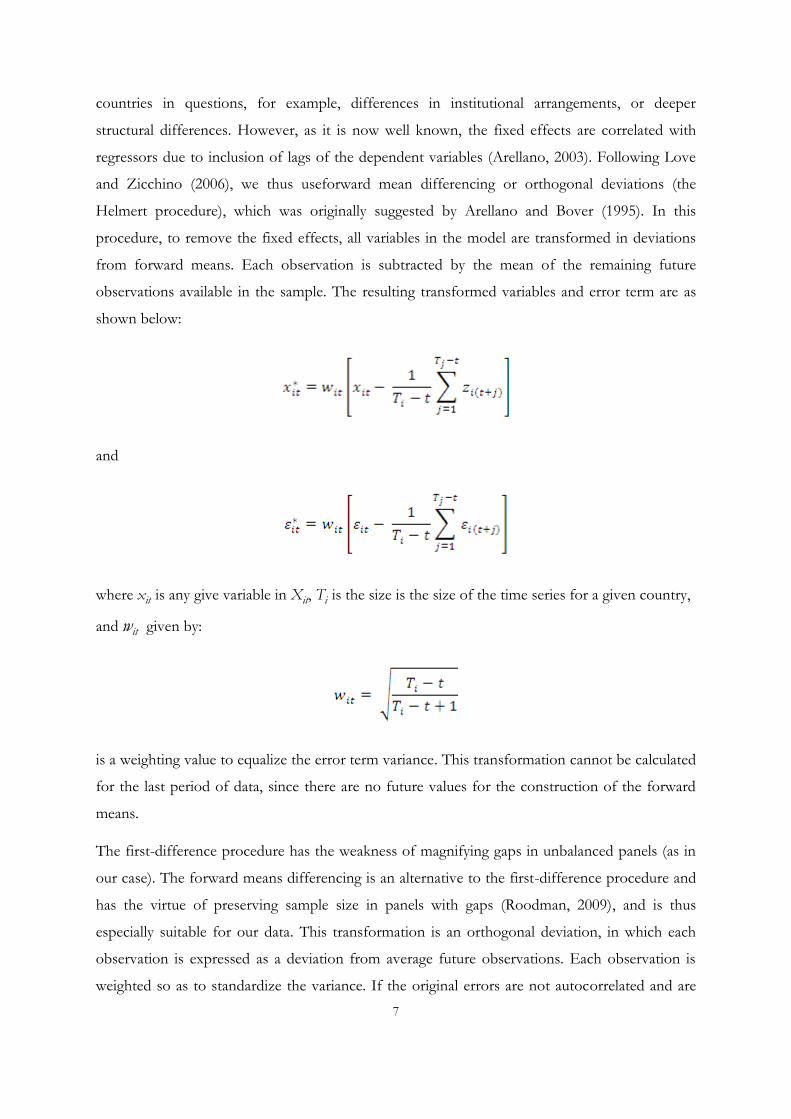
procedure, to remove the fixed effects, all variables in the model are transformed in deviations
from forward means. Each observation is subtracted by the mean of the remaining future
observations available in the sample. The resulting transformed variables and error term are as
shown below:
and
where xit is any give variable in Xit, Ti is the size is the size of the time series for a given country,
and wit given by:
is a weighting value to equalize the error term variance. This transformation cannot be calculated
for the last period of data, since there are no future values for the construction of the forward
means.
The first-difference procedure has the weakness of magnifying gaps in unbalanced panels (as in
our case). The forward means differencing is an alternative to the first-difference procedure and
has the virtue of preserving sample size in panels with gaps (Roodman, 2009), and is thus
especially suitable for our data. This transformation is an orthogonal deviation, in which each
observation is expressed as a deviation from average future observations. Each observation is
weighted so as to standardize the variance. If the original errors are not autocorrelated and are
8
characterized by a constant variance, the transformed errors should exhibit similar properties.
Thus, this transformation preserves homoscedasticity and does not induce serial correlation
(Arellano and Bover, 1995). Additionally, this technique allows use of the lagged values of
regressors as instruments, and estimates the coefficients by the generalized method of moment
(GMM).
In the sample, each variable in the VAR is time demeaned, i.e., for each time period. As in Love
and Zicchino (2006), the mean of the series across panels is computed and then subtracted from
the series. This iter removes the time specific effects and, thus, moderates the influence of cross-
sectional dependence on panel data (Levin et al., 2002). Using time demeaned series permits to
satisfy the above assumption of cross-sectionally uncorrelated error.
We estimate the model using generalized method of moments (GMM). The standard OLS
estimation methods are liable to lead to seriously biased coefficients in dynamic models (e.g.,
Nickell, 1981). In contrast, GMM is well suited for obtaining efficient estimators in a panel data
context where a model like ours contains lagged dependent variables along with unobserved
effects (e.g., Arellano and Bond, 1991).
The impulse response functions and error variance decompositions are often centred in VAR
analyses, which allow us to gain a clear picture of the dynamic relationships among variables of
interest. Particularly, the impulse response functions describe how one variable responds over
time to the innovations in other endogenous variables which are assumed to be uncorrelated
with other shocks in the system (while holding all other shocks equal to zero). The variance
decomposition shows how much of the error variance of each of the variables can be explained
by shocks to the other variables. Thus, the variance decomposition provides information about
the relative importance of each random innovation in affecting the variables in the system. To
better understand the implications of the impulse response functions, confidence bands are
warranted. We use Monte Carlo simulations to generate 1000 impulse responses based on the
estimated coefficients and their standard errors. The confidence bands are thus given by 2.5th
and 97.5th percentiles of the 1000 simulated impulse responses3.
3 In practice, we randomly generate a draw of coefficients Γ by employing the estimated coefficients and their
variance–covariance matrix and re-calculate the impulse-responses.

9
Once all the coefficients of the panel VAR are estimated, we compute the impulse response
functions (IRFs) and the variance decompositions (VDCs)4. In order to compute the IRFs we
use the Cholesky decomposition. Considering that the actual variance–covariance matrix of the
errors is unlikely to be diagonal, to isolate shocks to one of the variables in the system it is
necessary to decompose the residuals in such a way that they become orthogonal (i.e. Cholesky
decomposition). The assumption behind the Cholesky decomposition is that series listed earlier
in the VAR order impact the other variables contemporaneously, while series listed later in the
VAR order impact those listed earlier only with lag. Consequently, variables listed earlier in the
VAR order are considered to be more exogenous. The identifying restrictions on the order of
variables for our equations are based on the rationale suggested by the literature on the
mechanism of monetary/fiscal transmission and the determination of exchange rate and the
current account. The ordered list of the variables is {ΔGDP, ΔFD, ΔIR, ΔCA, ΔREER} where
the contemporaneously exogenous variables are ordered first. Following Kim and Roubini
(2008), we order the fiscal balance before the interest rate. This setup shares the same spirit with
van Aarle et al. (2003) in modelling monetary and fiscal policy transmission together. In the
model, the (exogenous) government deficit shocks are extracted by conditioning on the current
and lagged GDP and all other lagged variables. We condition on current GDP since the
government budget (deficit) is likely to be endogenously affected by the current level of
economic activity within a quarter. In particular, elements of government revenue, such as sales
taxes and income taxes, are very likely to depend on the current level of economic activity within
a quarter. In addition, the government budget deficit may also depend on the lagged level of
various variables. For example, some elements of government revenue, such as the income tax,
may depend on the lagged level of economic activity. However, we do not condition on current
variables other than the real GDP considering the nontrivial decision lags in fiscal policy. That is,
conditioning on the current real GDP is essential to control the current endogenous reactions of
the government primary deficit to current economic activity; while not conditioning on other
current variables is reasonable to identify exogenous or discretionary changes in the government
deficit since such changes are less likely to depend on other current variables because of the
decision lags of fiscal policy. The exchange rate is often assumed to be more endogenous,
allowing for an immediate reaction to policy shocks and other economic variables (e.g.,
Peersman and Smets, 2001; Kim and Roubini, 2008), which hinges on the insights provided by
4 The panel VAR is estimated using the package provided by M. Abrigo and I. Love (2015). This package is an
updated Stata program for Love (2001) and is also used in Love and Zicchino (2006).
10
canonical models of exchange rate determination such as Dornbusch’s overshooting model and
the monetary models of Frenkel and Mussa. Granger causality tests are also used to support the
ordering of the variables. Some of the variables exhibit feedback relationship, at which point
economic theory is also considered. The results of the Granger causality tests are provided in
Table 1.
In this study, imposing a long-run steady state relationship for the Central East European
countries may not be realistic as these emerging market economies have different growth paths
and their economic patterns may change substantially along the path. Therefore, we use the
unrestricted panel VAR model and rely exclusively on the data themselves to identify the
underlying structure.
IV. Data and Econometric Analysis
Data
Our analysis utilizes the dataset available from the Eurostat and IMF's International Financial
Statistics (IFS)5 for the countries: Albania, Bulgaria, Croatia, Czech Republic, Hungary,
Lithuania, Macedonia, Poland, Romania, Serbia and Turkey. We collect quarterly data on GDP
(index 2010=100), fiscal balance as percentage of GDP, short-term interest rate6, current account
balance as percentage of GDP, and real effective exchange index (see Table 2).
Fiscal balance is calculated as the difference between total revenue and total expenditure which
are compiled on a national accounts (ESA 2010) basis. The REER indexes for all the countries
under the study are constructed based on the computation of the nominal effective exchange
rate and consumer price, which states the price or relative cost between the country under review
and its trading partners:
5 We update, if appropriate, the data using resources from official websites of relevant countries, including central
bank websites.
6 For EU countries we have considered the 3-months money market interest rate, except Bulgaria. For the rest of
the countries the o/n interest rate has been considered.
11
where Pfn and P are foreign and domestic price indices, En is the nominal exchange rate for the
national and foreign currency expressed as the price of a foreign currency unit to the national
currency, and βn is the share of the relevant trading partner n in domestic trade.
The dataset is sampled from the first quarter of 2005 up to the last quarter of 2014, while the
Macedonias fiscal balance is only available starting 2008:Q1. Variables exhibit strong seasonality,
for which we seasonally adjusted7, and then transformed them into logarithms.
A striking advantage of using the structural fiscal balance as the fiscal policy indicator, instead of
the more conventional headline balance, is that it is cyclically-adjusted, allowing policymakers,
analysts and observers to more accurately assess the fiscal position net of cyclical effects. Public
revenues and expenditures are often affected substantially by the boom and bust cycle of the
economy in ways that are not related to the underlying fiscal position. Decreases in tax revenues
and increases in unemployment benefits spending during economic recessions, for instance, will
generally lead to a huge surge in government deficits, which indeed is not the result of a
deliberately expansive policy.
Of the 11 countries that are part of the panel, seven are EU members (Bulgaria, Croatia, Czech
Republic, Hungary, Poland, Romania, and Lithuania). Four countries, Bulgaria, Croatia,
Lithuania and Macedonia have a fixed exchange rate regime. Lithuania has become member of
the Eurozone only in January 2015 and this does not affect our panel data.
Panel unit root test and cointegration analysis
The first step of the analysis is to look at the properties of the data. Failing to account for these
properties of the data may lead to spurious or misleading characterization of the dynamic
relationships among variables. To date, several methods have been developed to test for unit
roots in panels, Levin, Lin, and Chu (2002, LLC) and Im, Pesaran and Shin (2003, IPS). The
LLC and IPS tests both maintain the null hypotheses that each series in the panel contains a unit
root, but the alternative of the LLC test requires each series to be stationary with an identical
autoregressive coefficient for all panel units while the alternative of the IPS test allows for some
(but not all) of the individual series to have unit roots; that is, the autoregressive coefficients are
heterogeneous. Hadri (2000) derives a residual-based test where the null hypothesis is that the
7 Variables are adjusted by using the Census XII multiplicative seasonal adjustment method used by the US Bureau
of Census.

12
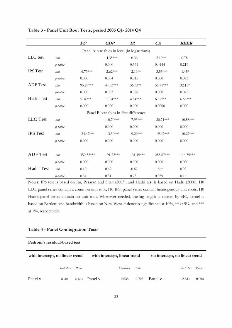
series are stationary against the alternative of a unit root in the panel. Table 3 reports the results
of the panel unit root tests based on different testing procedures. Levels of time series are found
to be nonstationary for the short-term interest rate and real exchange rate. According to the
Hadri approach all the variables are non-stationary. Nevertheless, it has been shown by
Hlouskova and Wagner (2006) that the Hadri test may suffer significant size distortion in the
presence of autocorrelation when the series does not contain a unit root. Indeed, Hlouskova and
Wagner find that the Hadri test tends to over-reject the null hypothesis of stationarity for all
processes that are not close to a white noise. However, the results show that all variables are
stationary in first-difference. Therefore, in our panel of 11 countries, we conclude that the
variables are non-stationary in level but stationary in first-difference.
Table 4 reports the results of the cointegration tests. These are error correction based panel
cointegration tests developed by Pedroni (1999) in order to check if long-run relationships exist
among integrated variables for selected countries. Pedroni (1999) develops two classes of
statistics to test for the null hypothesis of no cointegration in heterogeneous panels, namely
panel cointegration statistics (within-dimension) and group-mean cointegration statistics
(between-dimension), which allow for heterogeneity in cointegrating relationships across
members of the panel. As shown by the robust p-value, for most of the statistics considered, the
null hypothesis of no cointegration cannot be rejected. Therefore, the empirical properties of the
variables examined require estimation of the VAR in first differences, since no cointegration
relationships exist between the (non-stationary) variables (in level).
V. Empirical Results
This section presents the impulse response functions and the variance decomposition from the
panel VAR.
While the optimal VAR lag length in a standard VAR can be determined by statistical criteria,
this is not straightforward for the PVAR due to cross-sectional heterogeneity. Following Abrigo
and Love (2015), we apply the consistent moment and model selection criteria (MMSC) for
GMM models proposed by Andrews and Lu (2001), based on Hansen’s (1982) J statistic of over-
identifying restrictions. Their proposed MMSC are analogous to various commonly used
maximum likelihood-based model selection criteria, namely the Akaike information criteria (AIC)
(Akaike, 1969), the Bayesian information criteria (BIC) (Schwarz, 1978; Rissanen, 1978; Akaike,
1977), and the Hannan-Quinn information criteria (HQIC) (Hannan and Quinn, 1979). As an

13
alternative criterion, the overall coefficient of determination (CD) may be calculated even with
just-identified GMM models (see Table 5).
As in Abrigo and Love (2015), in our case the first-order panel VAR is the preferred model,
since this has the smallest MBIC, MAIC and MQIC. However, the over-all coefficient of
determination suggests applying a model with more than 1 lag. In addition, in most
macroeconomic analyses, a lag length of 1 or 2 is often regarded as too short to capture enough
economic interactions among variables for a model with quarterly data (see for example Kim and
Roubini, 2008). Balancing the need of allowing for a sufficient number of lags given the nature
of the data and trying to avoid overparametrization, we set the number of lags to 3, opting for a
third-order panel VAR model.
Impulse Response Function
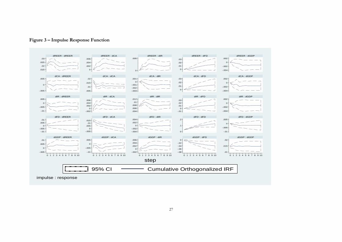
Figures 1 and 3 display the impulse response functions respectively for the current account and
for all the endogenous variable of the panel VAR model. The accumulated impulse responses
(solid line) are presented over time8. The confidence bands, given by 2.5th and 97.5th percentiles
of the 1000 simulated impulse responses are presented by the dash lines.
The response of the current account to interest rate shocks seems not to be statistically
significant. This seems to be consistent with the conclusions pointed out by Ferraro et al. (2010).
According to this study the behavior of international variables (such as current account and
exchange rate) is less sensitive to monetary policy compare to domestic variables9.
In relation to the exchange rate, a positive shock means a depreciation of the local currency. As
one can see, the response of the external balance to a real depreciation of domestic currency is
not immediate. The importance of the real shock in the first quarter is zero (see Table 7 on
variance decomposition), because the initial response is close to zero. It increases later, and is
8 For example, the first row in Figure 3 displays the effect of one standard deviation shock on real effective
exchange rate (REER) on itself and on the other endogenous variables.
9 The authors by employing two-country monetary DSGE model have pointed out that in case of a sharp current
account reversal (due to a sudden revision of the relative growth prospects of the home versus foreign country)
home central bank will raise interest rates sharply to avoid currency depreciation. However, by the other side, this
sharp increase in interest rates, in turn, causes a major contraction in aggregate economic activity within the home
country. The shrinkage is particularly relevant in the nontradable goods sector, pointing out the inefficient sectoral
reallocation.
14
statistically significant only after 4 quarters and the effect remains significant. As shown,
depreciation in the real exchange rate has a positive effect on these countries’ external balances
after a year. It is clear that some J-curve effect associated with this interaction is not missing for
the countries under review10.
In response to a positive output shock, the current account worsens. The effect is significant just
1 quarter after the shock and it is larger after 3 quarters. These results are not surprising and in
line with theoretical expectations that positive domestic economic output boosts demand for
foreign goods and services and consequently deteriorates the current account balance (see
Calderon et al., 2002; Aristovnik, 2008). Although an increase in domestic output can be
associated with a greater savings rate, it seems that the rise in consumption and investment
together are somewhat greater, thus leading to an expansion of the current account deficit
(Backus et al., 1994). This is also consistent with the findings of Aguiar and Gopinath 2007, who
report that emerging markets are characterized by strongly counter-cyclical current accounts.
It is interesting to note the positive relation between the current account balance and fiscal
balance. An improvement of the fiscal balance tends to have a positive effect on the current
account deficit. A variety of models predict a positive relationship between government budget
balances and current accounts over the medium term. Overlapping generations models suggest
that government budget deficits tend to induce current account deficits by redistributing income
from future to present generations (see Obstfeld and Rogoff, 1994 and Chinn, 2005). Only in the
particular case of full Ricardian equivalence, where private saving fully offsets changes in public
saving, would there be no link between government budget balances and current account
balances. Our result seems to confirm the Bussière et al., (2004) findings on the connection
between the government fiscal deficits and the current account (the idea of the “twin deficits”).
It seems also important to report how an improvement of fiscal balance has a negative and
significant impact on the GDP activity of this group of countries, consistent with standard
theory (for more details see Figure 3). By the other side, one can see that a positive growth of
10 Under the J-Curve phenomenon the trade balance of a given country follows an immediate deterioration after real
currency depreciation (short run deterioration combined with long-run improvement), due to some time lag
between order and delivery of imports. This is partly consistent with the immediate negative response of the terms
of trade to devaluation: the pass-through from a devaluation to export prices in the national currency is slower than
that to import prices in the national currency due to the missing price adjustment of domestic producers to get a
competitive advantage (Backus et al., 1994).

15
domestic output worsens the fiscal deficit by showing a permanent effect. This is consistent
especially for developing countries due to investment increasing.
Variance Decomposition
These results seem to be confirmed by the forecast-error variance decomposition (FEVD) based
on a Cholesky decomposition of the residual covariance matrix of the underlying panel VAR
model (see Table 7). The results contained in Table 7 show that the contribution of gross
domestic output (first column) and fiscal deficit (second column) explain 1.3% and 42.3% of the
variation of current account deficit just after one quarter. It finds that fiscal deficit seems to play
an especially important role in explaining the current account balance. After 10 quarters the
contribution of GDP increases somewhat (3.4%) and that of domestic interest rate and real
effective exchange rate both is 2.5%.
To check the robustness of our results, we perform again the IRF analysis using alternative
measures of external imbalances like the trade deficit (net exports). These results show that our
previous findings are robust to this alternative measure. Indeed, as before, trade deficit improves
in response to an appreciation of real effective exchange rate and a positive fiscal deficit shock
for the whole panel (see Figure 2).
VI. Concluding Remarks
This paper use a panel VAR model to empirically investigate the dynamic interactions between
monetary policy, fiscal policy, exchange rates, as well as their impacts on current account balance
in eleven emerging market economies in central and east Europe. The results are largely
consistent with the theoretical literature and previous empirical analysis. We found that fiscal
deficit worsening is likely to be accompanied with current account balance deterioration,
confirming the validity of the twin deficit hypothesis in the region. It shows that the fiscal deficit
is an important variable affecting the current account dynamics by explain between 40-42% of it
variance in a variance decomposition exercise. The results also show that an increase in domestic
GDP has a persistent negative effect on the current account balance, implying that the domestic
growth rate is associated with a larger increase in domestic investment than saving. Further, the
impulse response analysis shows that the depreciation of the real effective exchange rate does
not have an immediate effect on the current account, but can improve it after one year.

16
We improve on the existing literature in several directions. First, although cross-country
empirical studies are not missing, they are mainly focused on the advanced economies and
EU/EA countries. Our work is among the very few studies that focus on this sample of
developing market countries in East Europe by employing quarterly data. Trying to understand
the dynamic interactions between policy impacts, real economic activities, and external
imbalances for these counties may provide important insights into the main current account
drivers and policy coordination in the region. Moreover, taking into account the correlation
between fiscal and monetary policy, we have considered both fiscal and monetary policy
transmissions in unified framework. This is an additional contribution of our paper to the
literature on monetary and fiscal analysis.
Future work may build on our analysis in a number of ways. In primis further research remains
obviously needed in order to better understand the factors that lie behind the dynamic
interactions for this set of countries. In addition, while in this study no theoretical constrains has
been imposed, an analysis based on a Bayesian Panel VAR framework would present a further
step for future works.

17
References
Abbas A., Bouhga-Hagbe S. M., Fatás J., Mauro, P., and Velloso, R.C. (2010), “Fiscal policy and
the current account”, IMF Working Paper No. 10/121.
Abrigo M. and Love I. (2015). “Estimation of panel vector autoregression in Stata: a package of
programs”, http://paneldataconference2015.ceu.hu/Program/Michael-Abrigo.pdf.
Aguiar M., and Gopinath G., (2007), “Emerging market business cycles: the cycle is the trend”,
Journal of Political Economy, 115, 69-102.
Andrews D.W.K., and Lu B., (1999). “Consistent model and moment selection criteria for GMM
estimation with application to dynamic panel data models” Cowles Foundation Discussion Paper
No. 1233, Yale University.
Arellano M., (2003), “Modelling Optimal Instrumental Variables For Dynamic Panel Data
Models”, Working Papers wp2003_0310, CEMFI.
Arellano, M., and Bover, O. (1995), “Another look at the instrumental variable estimation of
errorcomponents models”, Journal of Econometrics, 68, 29–51.
Arellano, M., and Stephen R. B. (1991), “Some tests of specification for panel data: Monte Carlo
evidence and an application to employment equations”, Review of Economic Studies, 58:2, 277–
97.
Aristovnik A., (2008), “Fiscal Sustainability in the Mediterranean Region - A Comparison
between the EU and Non-EU Member States.” Romanian Journal of Economic Forecasting,
9(4): 161-173.
Aristovnik, A., (2008), “Short-term determinants of current account deficits”, Eastern European
Economics, vol. 46, no. 1, pp. 24-42.
Assenmacher-Wesche K., and Gerlach S., (2008), “Monetary policy, asset prices and
macroeconomic conditions: A panel VAR study”, Working Paper 149, National Bank of
Belgium.
Backus, D. K.,Kehoe, P. J. and Kydland F. E. (1994). Dynamics of the Trade Balance and the
Terms-oftrade: The J-Curve? American Economic Review, 84, 84-103.

18
Bini Smaghi L., (2007). "Global imbalances and monetary policy," Journal of Policy Modeling,
Elsevier, vol. 29(5), pages 711-727.
Blanchard O.J., and Milesi-Ferretti, G.M. (2010), “Global imbalances: in midstream?” Il SaKong,
Olivier
Boileau M., and Normandin M., (2004), “The Current Account and the Interest Differential in
Canada”, Cahiers de recherche 0424, CIRPEE.
Calderon C. A., Chong A., and Loayza N. V., (2002), "Determinants of Current Account Deficits
in Developing Countries", Contributions to Macroeconomics: Vol. 2: No. 1, Article 2.
Cheung, Y., Chinn, M.D., and Pascual, A.G. (2005). “Empirical exchange rate models of the
nineties: are they fit to survive? Journal of International Money and Finance, 24, 1150-1175.
Evans M. and Hnatkovska V., (2005), "International Capital Flows, Returns and World Financial
Integration," NBER Working Papers 11701, National Bureau of Economic Research, Inc.
Ferraro A., Mark G., and Svensson, L. (2010). “Current account dynamics and monetary policy”.
In Gali, J. and Gertler, M. (Eds.), International Dimensions of Monetary Policy, University of
Chicago Press, Chicago, IL (2010), 199–244.
Fidrmuc J., (2003), “The Feldstein–Horioka Puzzle and Twin Deficits in selected countries”,
Economic Change and Restructuring, vol. 36, no. 2, pp. 135-152.
Fratzscher M., Juvenalb, L, and Sarno, L. (2010), “Asset prices, exchange rates and the current
account, European Economic Review”, Vol 54, Issue 5, 643–658.
Frenkel J., and Razin A., (1996). "Fiscal Policies and Growth in the World Economy," MIT
Press Books,The MIT Press, edition 3, volume 1, number 0262561042, June.
Gavin W. and Theodorou A. (2005). “A common model approach to macroeconomics: using
panel data to reduce sampling error”, Journal of Forecasting, 24, 203-219.
Goodhart, C., and Hofmann, B. (2008). “House prices, money, credit, and the macro-economy”,
Oxford Review of Economic Policy, 24(1): 180-205.
Gupta D. D., and Ratha D., (2000), “What Factors Appear to Drive Private Capital Flows to
Developing Countries? And how Does Official Lending Respond?” Vol. 2392. World Bank
Publications.

19
Hadri, K. (2000), “Testing for stationarity in heterogeneous panel data”, Econometrics Journal 3:
148–161.
Harkmann K. and Staehr, K. (2012) Current account balances in Central and Eastern Europe:
Heterogenity, Persistence and Driving Factors, pp 15-16, accessed on March 2014 at
http://ies.fsv.cuni.cz/default/file/get/id/20935
Henry P. B., (2006), “Capital Account Liberalization: Theory, Evidence, and Speculation.”
NBER Working Paper no. w12698.
Hermann S., Jochem A., (2005), “Determinants of Current Account Developments in the
Central and East European EU Member States- Consequences for the Enlargement of the Euro
Area. Deutsche Bundesbank, Paper Series 1: Economic Studies. No: 32/2005.
Herrmann S., and Winkler A., (2008), “Real Convergence, Financial Markets and the Current
Account – Emerging Europe versus Emerging Asia”. ECB Occasional Paper 88.
Hlouskova J., and Wagner M., (2006), “The performance of panel unit root and stationarity tests:
Results from a large scale simulation study”, Econometrics Reviews, 25, 85-116.
Im K.S., Pesaran M.H., and Shin Y., (2003), “Testing for unit roots in heterogeneous panels”,
Journal of Econometrics 115: 53–74.
Kim S., and Roubini, N., (2008), “Twin deficit or twin divergence? Fiscal policy, current account,
and real exchange rate in the U.S”, Journal of International Economics, 74, 362-383.
Lane P., (2008), “The Macroeconomics of Financial Integration: A European Perspective”, IIIS
Discussion Paper 265.
Lane P., and Milesi-Ferretti G.M., (2006), “Exchange Rates and External Adjustment: Does
Financial Globalization Matter?”, The Institute for International Integration Studies Discussion
Paper Series, IIIS.
Lee J., and Chinn M.D., (2006), “Current account and real exchange rate dynamics in the G7
countries”, Journal of International Money and Finance, 25, 257-274.
Levin A., Lin C.F., and Chu C.S.J. (2002), “Unit root tests in panel data: Asymptotic and finite-
sample properties”, Journal of Econometrics 108: 1–24.
Love I., and Zicchino L., (2006), “Financial development and dynamic investment behaviour:
Evidence from panel VAR”, The Quarterly Review of Economics and Finance, 46, 190-210.
20
Monacelli T., and Perotti R., (2007) “Fiscal Policy, the Trade Balance, and the Real Exchange
Rate: Implications for International Risk Sharing”, 8TH Jacques Polak Annual Research
Conference.
Monacelli T., and Perotti, R. (2010), “Fiscal policy, the real exchange, and traded goods”,
Economic Journal, 120:437–461.
Mundell R. A., (1960), “The Monetary Dynamics of International Adjustment under Fixed and
Flexible Exchange Rates,”Quarterly Journal of Economics,Vol. 74 (May), pp. 227–57.
Nickell S., (1981), “Biases in dynamic models with fixed effects”, Econometrica 49, 1417-1426.
Obstfeld M., and Rogoff K., (1994), “The Intertemporal Approach to the Current Account”,
Center for International and Development Economics Research (CIDER) Working Papers C94-
044, University of California at Berkeley.
Obstfeld M., and Rogoff, K. (2009), “Global imbalances and the financial crisis: products of
common causes”, CEPR Discussion Paper, No. 7606.
Paleologos J., and Bitzis G., (2006), “Assessing the Effectiveness of the Exchange Rate
Movements on the Greek Current Account Deficit: A Cointegration Analysis”, European
Research Studies Journal, European Research Studies Journal, vol. 0(1-2), pages 45-64.
Pedroni P. (1999), “Critical values for cointegration tests in heterogeneous panels with multiple
regressors”, Oxford Bulletin of Economics and Statistics, 61, Special Issue, 653-670.
Peersman G., and Sets F., (2001), “The monetary transmission mechanism in the euro area: more
evidence from VAR analysis”, European Central Bank Working Paper Series, NO. 91.
Prasad E., Kenneth R., Wei Sh. J., and Kose M., (2003), “Effects of Financial Globalization on
Developing Countries: Some Empirical Evidence.” International Monetary Fund.
Rahman J., (2008), “Current Account Developments in New Member States of the European
Union: Equilibrium, Excess and EU-phoria”, IMF Working Paper, No. 08/92,
Rahman M., (2008), “The Impact of a Common Currency on East Asian Production Networks
and China’s Exports Behavior”, MPRA Paper 13931, University Library of Munich, Germany.
Ravn M., Schmitt-Grohe S., and Uribe M., (2007), “Incomplete Cost Pass-Through Under Deep
Habits”, NBER Working Papers 12961, National Bureau of Economic Research, Inc.

21
Roodman D., (2009), “A Note on the Theme of Too Many Instruments”, Oxford Bulletin of
Economics and Statistics, Department of Economics, University of Oxford, vol. 71(1), pages
135-158, 02.
Roubini N., and Wachtel P., (1998), “Current Account Sustainability in Transition Economies",
NBER Working Papers 6468, National Bureau of Economic Research, Inc.
Salter W., (1959). “Internal and External Balance: The Role of Price and Expenditure Effects”,
Economic Record, Volume 35 Issue 71 pg 226-238.
van Aarle V., Garretsen, H., and Gobbin, N., (2003), “Monetary and fiscal policy transmission in
the Euroarea: evidence from a structural VAR analysis”, Journal of Economics and Business, 55,
609-638.
Winfried K., Bussiere M., and Fratzscher M., (2004). “Currency Mismatch, Uncertainty and Debt
Structure”, Econometric Society 2004 North American Summer Meetings 181, Econometric
Society.

22
Appendix
Table 1 - Panel VAR-Granger causality Wald test
Equation/Excluded Prob. Equation/Excluded Prob. Equation/Excluded Prob.
dGDP
dFD
dIR
dCA
dREER
ALL
0.846
0.107
0.069
0.915
0.091
dFD
dGDP
dIR
dCA
dREER
ALL
0.002
0.712
0.275
0.531
0.003
dREER
dGDP
dFD
dIR
dCA
ALL
0.558
0.874
0.057
0.334
0.268
dIR
dGDP
dFD
dCA
dREER
ALL
0.039
0.880
0.159
0.012
0.000
dCA
dGDP
dFD
dIR
dREER
ALL
0.050
0.017
0.088
0.114
0.002
Notes: Ho: Excluded variable does not Granger-cause Equation variable and Ha: Excluded variable Granger-causes Equation
variable.
Table 2 – Descriptive Statistics
Variable Mean Std dev. Min Max N.obs.
Real GDP 4.604 0.081 4.322 4.839 440
Fiscal Deficit -0.029 0.035 -0.200 0.072 428
Interest Rate 0.053 0.038 0.000 0.179 440
Current Account -0.057 0.060 -0.270 0.106 440
Real Effective Exchange Rate 4.589 0.082 4.347 4.85 440
23
Table 3 - Panel Unit Root Tests, period 2005 Q1- 2014 Q4
Notes: IPS test is based on Im, Pesaran and Shan (2003), and Hadri test is based on Hadri (2000). H0
LLC: panel series contain a common unit root; H0 IPS: panel series contain heterogenous unit roots; H0
Hadri: panel series contain no unit root. Whenever needed, the lag length is chosen by SIC, kernel is
based on Bartlett, and bandwidth is based on New-West. * denotes significance at 10%, ** at 5%, and ***
at 1%, respectively.
Table 4 - Panel Cointegration Tests
Pedroni’s residual-based test
with intercept, no linear trend with intercept, linear trend no intercept, no linear trend
Statistics Prob. Statistics Prob. Statistics Prob.
Panel v- 0.981 0.163 Panel v- -0.538 0.705 Panel v- -2.511 0.994
FD GDP IR CA REER
Panel A: variables in level (in logarithms)
LLC test stat -4.35*** -0.36 -2.19** -0.78
p-value 0.000 0.361 0.0144 0.219
IPS Test stat -6.73*** -2.62*** -2.16** -3.55*** -1.45*
p-value 0.000 0.004 0.015 0.000 0.073
ADF Test stat 95.29*** 44.03*** 36.33** 55.71*** 32.15*
p-value 0.000 0.003 0.028 0.000 0.075
Hadri Test stat 5.04*** 11.04*** 4.64*** 6.37*** 6.66***
p-value 0.000 0.000 0.000 0.0000 0.000
Panel B: variables in first difference
LLC Test stat -10.70*** -7.93*** -20.71*** -10.58***
p-value 0.000 0.000 0.000 0.000
IPS Test stat -24.47*** -13.30*** -9.29*** -19.67*** -10.27***
p-value 0.000 0.000 0.000 0.000 0.000
ADF Test stat 350.32*** 191.22*** 131.49*** 288.67*** 144.39***
p-value 0.000 0.000 0.000 0.000 0.000
H adri Test stat 0.40 0.49 -0.67 1.56* 0.99
p-value 0.34 0.31 0.75 0.059 0.16

24
Statistic Statistic Statistic
Panel rho-
Statistics -1.112 0.133
Panel rho-
Statistics 0.579 0.719
Panel rho-
Statistics 0.349 0.637
Panel PP-
Statistics -1.269 0.102
Panel PP-
Statistics -0.053 0.478
Panel PP-
Statistics 0.363 0.642
Panel ADF-
Statistics -2.756 0.003
Panel ADF-
Statistics -3.185 0.000
Panel ADF-
Statistics -0.101 0.496
Group rho-
Statistics 0.136 0.554
Group rho-
Statistics 2.111 0.9826
Group rho-
Statistics 2.309 0.989
Group PP-
Statistics -0.609 0.271
Group PP-
Statistics 1.612 0.946
Group PP-
Statistics 1.335 0.909
Group ADF-
Statistics -2.991 0.002
Group ADF-
Statistics -1.436 0.076
Group ADF-
Statistics 0.828 0.796
Notes: Pedroni test is based on Pedroni (1999). The null hypothesis of all Pedroni's statistics is no
cointegration. The panel cointegration statistics (within dimension) require a common value in
cointegration while group-mean cointegration statistics (between-dimension) do not.
Table 5 – Panel VAR Selection Order Criteria
Table 6 - Stability condition test
Eigenalue Modulus
Real Imaginary
0.847 0 0.847
0.375 0.502 0.627
0.375 -0.502 0.627
Lag CD J J pvalue MBIC MAIC MQIC
1 0.899 122.19 0.0005 -319.69 -27.81 -143.84
2 0.938 98.10 0.00006 -196.48 -1.89 -79.25
3 0.957 53.00 0.0009 -94.28 3.01 -35.67
4 0.968 0.00 0.00 0.00 0 0

25
-0.319 0.477 0.574
-0.319 -0.477 0.574
0.363 -0.416 0.552
0.363 0.146 0.552
-0.529 0 0.529
-0.409 0.186 0.449
-0.49 -0.186 0.449
0.281 0.348 0.448
0.281 -0.348 0.448
-0.309 0.300 0.431
-0.309 -0.300 0.431
0.24 0 0.241
Table 7 – Current Account Balance Variance Decomposition
Period GDP FD IR CA REER
1 0.013 0.423 0 0.564 0
2 0.011 0.400 0.014 0.570 0.004
3 0.027 0.398 0.015 0.556 0.004
4 0.027 0.0393 0.018 0.554 0.007
5 0.033 0.392 0.019 0.549 0.007
6 0.032 0.393 0.019 0.548 0.008
7 0.033 0.393 0.019 0.546 0.008
8 0.034 0.394 0.019 0.545 0.008
9 0.034 0.394 0.019 0.545 0.008
10 0.034 0.395 0.019 0.544 0.008

26
Figure 1 – Impulse Response Function: current account
-.001
0
.001
.002
.003
.004
.005
.006
.007
.005
.01
.015
.02
-.002
0
.002
.004
.006
-.005
0
.005
.01
.015
-.01
-.005
0
.005
0 1 2 3 4 5 6 7 8 9 10 0 1 2 3 4 5 6 7 8 9 10
0 1 2 3 4 5 6 7 8 9 10
dREER : dCA
dCA : dCA
dIR : dCA
dFD : dCA
dGDP : dCA
95% CI Cumulative Orthogonalized IRF
step
impulse : response
Figure 2 - Impulse Response Function: trade balance
0
.002
.004
.006
.005
.01
.015
.02
-.002
0
.002
.004
-.005
0
.005
.01
-.006
-.004
-.002
0
.002
0 1 2 3 4 5 6 7 8 9 10 0 1 2 3 4 5 6 7 8 9 10
0 1 2 3 4 5 6 7 8 9 10
dREER : dTB
dTB : dTB
dIR : dTB
dFD : dTB
dGDP : dTB
95% CI Cumulative Orthogonalized IRF
step
impulse : response
27
Figure 3 – Impulse Response Function
.015
.02
.025
.03
-.005
0
.005
-.01
-.005
0
.005
-.01
-.005
0
.005
.01
-.005
0
.005
.01
0
.002
.004
.006
.005
.01
.015
.02
-.002
0
.002
.004
.006
-.005
0
.005
.01
.015
-.01
-.005
0
.005
0
.005
-.003
-.002
-.001
0
.001
.004
.006
.008
.01
.012
-.004
-.002
0
.002
.004
-.002
0
.002
.004
.006
0
.01
.02
.03
0
.01
.02
.03
-.01
0
.01
.02
.03
0
.1
.2
-.08
-.06
-.04
-.02
0
-.004
-.002
0
.002
-.004
-.002
0
.002
-.004
-.002
0
.002
-.01
-.005
0
.005
.01
.015
.02
0 1 2 3 4 5 6 7 8 9 10 0 1 2 3 4 5 6 7 8 9 10 0 1 2 3 4 5 6 7 8 9 10 0 1 2 3 4 5 6 7 8 9 10 0 1 2 3 4 5 6 7 8 9 10
dREER : dREER
dCA : dREER
dIR : dREER
dFD : dREER
dGDP : dREER
dREER : dCA
dCA : dCA
dIR : dCA
dFD : dCA
dGDP : dCA
dREER : dIR
dCA : dIR
dIR : dIR
dFD : dIR
dGDP : dIR
dREER : dFD
dCA : dFD
dIR : dFD
dFD : dFD
dGDP : dFD
dREER : dGDP
dCA : dGDP
dIR : dGDP
dFD : dGDP
dGDP : dGDP
95% CI Cumulative Orthogonalized IRF
step
impulse : response