CURRENCY RISK IN EMERGING EQUITY MARKETS

Kate Phylaktis* Fabiola Ravazzolo

Cass Business School Allianz Dresner Asset ManagementFrobisher Crescent Nymphenburger Strasse 112-116Barbican Centre 80636 MunichLondon EC2Y 8HB GermanyFax: (44) 020 7040 8881 Fax: (49) 89 1220 7799Email: K.Phylaktis@city.ac.uk Email: F.Ravazzolo@dit.de

JEL Classification Numbers: F31, G12

Keywords: International capital asset pricing models (ICAPM); currency risk; capitalmarket integration; emerging markets; and Pacific Basin capital markets.

Abstract

The paper develops an international capital asset pricing model, which includesforeign currency risk, and examines the impact of capital market liberalisation on thepricing of risks. It applies the model to data from Pacific Basin financial markets andfinds substantial evidence that not only currency risk is priced in both pre and postliberalisation periods, but the model is superior to one which does not includecurrency risk. This evidence suggests that an international capital asset pricingmodel, which omits currency risk, will be misspecified. Furthermore, the resultsimply that since currency risk is priced and investors are compensated for bearingsuch risk they should not be discouraged by more flexible exchange rate regimes frominvesting in emerging markets.

* Correspondence to: Kate Phylaktis

2

1. Introduction

The recent emergence of highly remunerative equity markets, following the relaxation

of foreign investment restrictions, and the developments in communication and

trading systems, has attracted the attention of academics to explain their impressive

returns. Their low correlation with the developed financial world has also intensified

the interest of international fund managers as opportunities for portfolio

diversification benefits. Evidence of that is the increasing flow of funds from

developed countries towards the newly established financial markets.1 The adoption

of more flexible exchange rate regimes by many emerging economies however in the

late eighties and early nineties is likely to have affected the foreign currency risk

associated with international investment and to have made the choice of currency

denomination an important element in the overall portfolio decision.

The objective of this paper is to develop an international capital asset pricing

model, which includes currency risk, and to examine the impact of capital market

liberalisation on the pricing of risks. Previous capital asset pricing models can be

classified into three groups based on the type of risk considered in pricing expected

returns: segmented market models, integrated market models, and partially segmented

market models. The segmented market model evaluates expected equity returns as a

function of only the country-specific risk represented by stock returns variance. A

classic segmented market framework is the Capital Asset Pricing Model (CAPM) of

Sharpe (1964), Lintner (1965) and Black (1972), applied to one country’s data. Such

We are grateful to the Emerging Markets Group, (EMG) Cass Business School,

London, (the new name for City University Business School), for financial support.

1 See e.g. Hawawini (1994) for evidence on the increasing flow of funds to new

capital markets and the importance of these markets to portfolio management.

3

a framework is suitable if the market is completely segmented or if it represents a

proxy for the world market. The suitability of this model has however diminished

over the years as the market capitalisation of any one single market as a proportion of

the world market has decreased. Within the class of asset-pricing models for

integrated markets there are studies that assume that all the world capital markets are

perfectly integrated, and therefore the source of their risk can be associated with the

covariance of the local stock market returns with the world market portfolio. These

include studies of an international CAPM (see Grauer, Litzenberger and Stehle,

1976); a world consumption-based model (see Wheatley, 1988); world arbitrage

pricing theory (see Solnik,1983); world multibetas models (see Ferson and Harvey,

1993 and 1994); and world latent factor models (see Campbell and Hamao, 1992 and

Bekaert and Hodrick, 1992). The polar approaches have produced on the whole poor

results. An alternative asset pricing model (see Errunza, Losq, and Padmanabhan,

1992) considers a framework in which the polar segmented/integrated cases are

replaced by a mild segmentation structure. While this model presents the advantage

of avoiding the choice between the scenario of full segmentation and perfect

integration, the framework has the disadvantage of selecting a degree of segmentation

that is fixed through time.

Errunza, Losq, and Padmanabhan's limitation has recently been overcome by

Bekaert and Harvey (1995) and De Santis and Imrohoroglu (1997). Bekaert and

Harvey (1995) proposed a one-factor asset pricing model that allows the conditional

expected returns of a country to be affected by their covariance with a world

benchmark portfolio and by the variance of the country returns. If the market was

perfectly integrated then only the covariance counted; while if the market was

completely segmented then the variance was the relevant measure of market risk.

4

Bekaert and Harvey (1995) use a conditional regime-switching model to account for

periods when national markets were segmented from world capital markets and when

they became integrated later in the sample. They applied the model to monthly

observations of equity returns of a group of emerging capital markets including the

countries in our sample, over the period 1975 to 1992. They found that integration

was substantial also for countries presenting extensive foreign ownership restrictions,

such as Korea and Taiwan.

De Santis and Imrohoroglu (1997) considering a group of emerging equity

markets covering the regions of Latin America, Middle-East and Asia for the period

December 1988 to May 1996, use the CAPM framework to study the stock returns

and the volatilities of these capital markets under different degrees of integration.

They introduce a dynamic integration version of the classic CAPM framework that

assumes full market segmentation until the official liberalisation date of each capital

market, and full integration thereafter to capture the fact that the analysed markets

were legally segmented for part of the sample period. The evidence shows that

neither the country specific risk is priced when are markets are segmented, nor the

world market risk when the markets are integrated.2

De Santis and Imrohoroglu's weak findings might be affected by two

limitations in their methodology. First, in contrast to Bekaert and Harvey (1995), the

date when each country switches from being fully segmented to being fully integrated

is fixed and the process is irreversible. Secondly, the lack in pricing the country-

specific risk might have been caused by the omission of currency risk, which affects

the expected returns of the local stock market. Dumas (1994) shows theoretically,

2 Country specific risk is not priced even when market segmentation is assumed for

the whole sample period.

5

while Dumas and Solnik (1995) empirically, that by applying the International CAPM

(ICAPM) framework with currency risk the latter is priced.

Dumas (1994) notes that if Purchasing Power Parity (PPP) does not hold, the

rates of inflation in the various countries, all expressed in U.S. dollars, are not equal

and their differences are random. On this point, Solnik shows that this is entirely

reflected by the random fluctuations of each currency against the dollar (see Solnik,

1974). Therefore, if PPP does not hold, any investment in a foreign asset is a

combination of an investment in the performance of the foreign asset and an

investment in the performance of the domestic currency relative to the foreign

currency. Thus, in applying international capital asset pricing models one should

endeavour to price it as its omission might bias findings.

Dumas and Solnik (1995) using the conditional version of ICAPM based on a

methodology originally proposed by Harvey (1991) show that the currency risk is

significantly different from zero for a sample of securities in Germany, US, Japan and

UK for the period March 1970 to December 1991. De Santis and Gerard (1998)

consider also a conditional version of the ICAPM based on multivariate GARCH,

which includes the foreign exchange risk for equity markets and one-month

Eurocurrency deposits for the same group of countries examined by Dumas and

Solnik (1995) but for the period June 1973 to December 1994. The results indicate

that investors require a premium for bearing currency risk. 3

3 Carrieri (2001) repeats the same analysis of De Santis and Gerard (1998), but for

France, Italy, Germany and U.K., using monthly observations for the period March

1974 to August 1995. She finds also that the currency risk is priced for these

European equity returns.

6

Based on the results about the importance of currency risk, our paper extends

the dynamic integration conditional CAPM of De Santis and Imrohoroglu (1997) by

including currency risk. We conduct our analysis by considering the same Asian

Pacific countries (with the only exception of India) analysed by De Santis and

Imrohoroglu, 1997), but extend the sample period from January 1980 to May 2000,

compared to their sample period of December 1988 to December 1996. Our analysis

shows that the limited relationship found in De Santis and Imrohoroglu (1997)

between risk and returns was due to the omission of currency risk.4

Thus, our main objective and contribution to the literature is the examination

of the importance of currency risk in explaining the stock returns of emerging equity

markets using a framework which allows for a regime switch in the sources of risk

affecting stock returns when they become open to foreign investors. Although our

model (as is De Santis and Imrohoroglu’s) is limited by the assumption that the date

when each country switches from being fully segmented to being fully integrated is

fixed and the process is irreversible, studies, such as Bekaert and Harvey (1995),

which allows for time–vaying integration, does not consider foreign currency risk.

Our approach of incorporating currency risk within an ICAPM framework is in fact a

variation of De Santis and Gerard (1998). Our specification, however, reflects the

limitations of data availability regarding suitable series for interest rates.

4 Asian Capital markets (Indonesia, Korea, Malaysia, Philippines, Singapore, Taiwan

Province of China and Thailand) have attracted substantial capital flows during the

1990’s. For example, in 1996, 48 percent of the net private capital flows to all

emerging economies was directed to these markets (see World Economic Outlook,

October 2000, published by the International Monetary Fund).

7

The paper is structured as follows. Section 2 explains the dynamic integration

asset-pricing model of equity returns with and without currency risk. It also

introduces the dynamic integration asset-pricing model for the currency returns.

Finally, it explains the estimation method of their conditional variances and

covariances by using a trivariate Generalised Autoregressive Heteroskedastic

(GARCH) process. Section 3 reports the summary statistics of each variable and

background information on the liberalisation of the financial markets in our sample.

Section 4 discusses the empirical results. The final section summarises the main

findings and offers some concluding remarks.

2. The model

2.1 Dynamic integration ICAPM with market and currency risks

The static version of CAPM whereby the expected return on the equity index of

country i is a linear function of the covariance between the return on that asset and the

return on the market portfolio can be given below when applying the GARCH

methodology

Et-1(Ri,t) = m10,i + m11,iRi,t-1 + m15,ihim,t, (1)

where him, t represents the conditional covariance between the return on index i and

the return on the world market portfolio. An autoregressive component is introduced

to take into account the effect of non-synchronous trading in the assets that make up a

market index, which is a usual phenomenon in emerging markets.5

The choice of the component representing the market risk depends on the

degree of financial integration of the analysed country. In a completely segmented

5 Following Black (1972) a risk-free rate is not included. That is due to the lack of a

monthly such rate for our sample period for the countries in this study.

8

capital market, the expected returns on the local market index is only associated with

the country-specific risk, which is proxied by the conditional variance of its equity

index returns. Under this scenario the expected return on an equity market i is

expressed as follows by modifying equation (1)

Et-1(Ri,t) = m10,i + m11,i Ri,t-1 + m12,ihii,t, (2)

where hii,t is the conditional variance of the market index of country i. In equation (2)

it is expected to obtain a significant and positive value for the coefficient m12,i, which

indicates that investors require higher expected returns when the market risk

increases. In contrast, under the scenario of a fully-integrated capital market, the

source of risk of the expected return of country i index is affected by its covariance

with the world market portfolio returns. This parameterisation has been reported in

equation (1), where him,t indicates the covariance between the returns of market index

i and the returns of a selected world market portfolio.

However, when examining emerging markets the degree of their integration

might not be identified by one of the two polar scenarios of perfect segmentation and

perfect integration. Therefore, in this case it is more appropriate to consider a

dynamic integrated CAPM framework. De Santis and Imrohoroglu (1997) introduced

a structure that allows in a single model a situation of full market segmentation until

the official liberalisation date, and full integration thereafter. The model is as follows

Et-1(Ri, t) = m10,i + m11,i Ri,t-1 + m12,ihii,t DCi,t + m15,ihim,t(1-DCi,t), (3)

where DCi is a dummy variable, which is equal to one before the opening date of

market i to foreign investors and zero otherwise. The dynamic integration framework

of equation (3) assumes that the price of risk is country-specific before liberalisation,

which is represented by the conditional variance of market index i, hii,t, and world

9

market when markets become integrated, which is indicated by the covariance of the

returns of market index i and the world market portfolio, him,t.

As it was mentioned before, one of our contributions to the literature is the

incorporation of the currency risk in the dynamic integration ICAPM framework.

This source of risk is important since PPP does not hold and investors of diverse

countries appreciate differently the real returns from the same securities. According

to Dumas (1994), the expected nominal rate of return on the market index of country

i, expressed in dollar units, using the ICAPM, is as follows (see Appendix A for

details of the derivation of this framework)

Et-1(Ri$,t) = r + bi cov(Ri$,t, Xi$,t) + ci cov(Ri$,t, Rm,t), (4)

where the two market premiums are related to the market i’s covariance with the rate

of appreciation of the currency of country i with respect to the U.S. dollar (cov(Ri$,t,

Xi$,t)) and to the covariance with the dollar rate of return on the optimal portfolio held

by investors of country i (cov(Ri$,t, Rm,t)). b and c relate to the market’s risk

aversion. The variable Xi$,t indicates the rate of change of the spot exchange rate

expressed in dollars per unit of nondollars currency of country i and r indicates the

nominal riskless rate of return for country i.

We use the two factor asset pricing model of equation (4) to derive the

ICAPM introduced in equations (1) and (2), but include the currency risk under the

scenarios of perfect segmentation and perfect integration (see Appendix B). On the

basis of the two polar cases, we derive the dynamic integration ICAPM of equation

(3) inclusive of currency risk by allowing full segmentation until liberalisation

(equation (5)) and perfect integration thereafter (equation (6)). The two polar cases

are given below

10

Et-1(Ri$, t)=m10,i + kti

p

kik Rm −

=∑ $,

1,11 + m12,ihii,t+ m13,ihxx,t+ 2m14,ihix,t , (5)

Et-1(Ri,$t) = m10,i + kti

p

kik Rm −

=∑ $,

1,11 + m15,ihim,t + m16,i hxm,t + m17,ihix,t

+ m18,ihxx,t. (6)

Bearing in mind that the rate of return of market index i expressed in US dollars is

equal to the return in local currency plus the change in the exchange rate (see B.3 in

Appendix B), the dynamic integration ICAPM process inclusive of currency risk that

we estimate is

Ri,t = m10,i - Xi$,t + )( $,,1

,11 ktikti

p

kik XRm −−

=

+∑ + m12,ihii,tDCi,t + m13,ihxx,tDCi,t

+ 2m14,ihix,tDCi,t + m15,ihim,t(1-DCi,t) + m16,ihxm,t(1-DCi)

+ m17,ihix,t(1-DCi,t) + m18,ihxx,t(1-DCi,t) + ε1,t, ( )t1tt,1 H,0N~I −ε (7)

where Ri,t represents the rate of return on market index i expressed in local currency;

Xi$ indicates the rate of appreciation of the local currency against the U.S. dollar; hii is

the variance of the returns expressed in local currency of the market index i; hxx is the

variance of the rate of appreciation (depreciation) of the local currency against the US

dollar; hix is the covariance of the returns expressed in local currency of market index

i with the rate of appreciation (depreciation) of the local currency with respect to the

US dollar; him is the covariance of the returns expressed in local currency of market

index i with the world market portfolio; and hxm is the covariance between the world

market portfolio and the rate of appreciation (depreciation) of the local currency

against the US dollar. DCi is a dummy variable that assumes the value of one before

liberalisation and zero otherwise. Ht is the conditional covariance matrix, which will

be discussed in section 2.2.

11

In estimating equation (7) we impose the condition that the coefficients m12,i

and m15,i are positive by taking their absolute value as a higher level of country-

specific or world market risk can only be compensated by higher stock returns. In

contrast, a linear specification is adopted for the currency risk (i.e. for m13,i, and m18,i)

as theory does not preclude the price of currency risk to be negative. According to

Glosten et al. (1993) investors may not require a high risk premium if the risky time

periods coincide with periods when investors are better able to bear particular types of

risk (as might be the currency one). Furthermore, if the future seems risky the

investor may want to save more in the present thus lowering demand for larger

premia. Therefore, both a positive and a negative relationship between stock returns

and these risks are possible. The prices of covariances (i.e. m14,i, m16,i , m17,i ) will be

discussed later on.

In our analysis we are also interested in modelling the rate of appreciation of

the local currency against the U.S. dollar. In particular, we use the risk-adjusted

uncovered interest rate parity (UIRP) condition introduced by Dumas (1994), to

derive the structures under the scenarios of full segmentation and full integration. We

proceed by combining the two polar cases to obtain the dynamic integration model,

which allows full segmentation before liberalisation and full integration thereafter.

The rate of appreciation of the local currency against the U.S. dollar, in the case of

full segmentation is given as follows (see Appendix B.3 for details of the derivation)

Xi$,t = m20,i + kti

p

kik Xm −

=∑ $,

1,21 + m22,ihxx,t + m23,ihix,t + ε2,t, ( )t1tt,2 H,0N~I −ε

(8)

under the case of full integration is given as

Xi$,t = m20,i + kti

p

kik Xm −

=∑ $,

1,21 + m24,i hxx,t + m25,ihmx,t + ε2,t, ( )t1tt,2 H,0N~I −ε

12

(9)

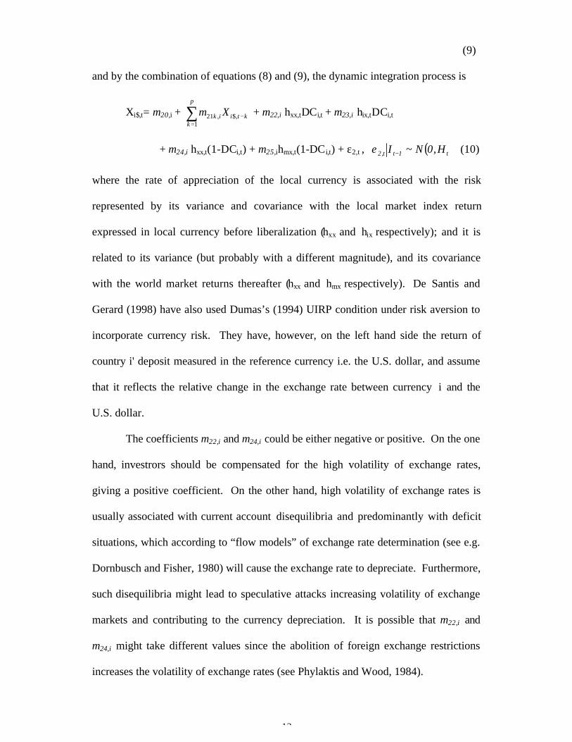
and by the combination of equations (8) and (9), the dynamic integration process is

Xi$,t= m20,i + kti

p

kik Xm −

=∑ $,

1,21 + m22,i hxx,tDCi,t + m23,i hix,tDCi,t

+ m24,i hxx,t(1-DCi,t) + m25,ihmx,t(1-DCi,t) + ε2,t , ( )t1tt,2 H,0N~I −ε (10)

where the rate of appreciation of the local currency is associated with the risk

represented by its variance and covariance with the local market index return

expressed in local currency before liberalization (hxx and hix respectively); and it is

related to its variance (but probably with a different magnitude), and its covariance

with the world market returns thereafter (hxx and hmx respectively). De Santis and

Gerard (1998) have also used Dumas’s (1994) UIRP condition under risk aversion to

incorporate currency risk. They have, however, on the left hand side the return of

country i' deposit measured in the reference currency i.e. the U.S. dollar, and assume

that it reflects the relative change in the exchange rate between currency i and the

U.S. dollar.

The coefficients m22,i and m24,i could be either negative or positive. On the one

hand, investrors should be compensated for the high volatility of exchange rates,

giving a positive coefficient. On the other hand, high volatility of exchange rates is

usually associated with current account disequilibria and predominantly with deficit

situations, which according to “flow models” of exchange rate determination (see e.g.

Dornbusch and Fisher, 1980) will cause the exchange rate to depreciate. Furthermore,

such disequilibria might lead to speculative attacks increasing volatility of exchange

markets and contributing to the currency depreciation. It is possible that m22,i and

m24,i might take different values since the abolition of foreign exchange restrictions

increases the volatility of exchange rates (see Phylaktis and Wood, 1984).

13

The prices of covariances between stock and foreign exchange returns in

equations (7) and (10) can also take either positive or negative values. There are two

channels connecting the foreign exchange market and the domestic and foreign stock

markets. On the one hand, the exchange rate affects the stock market through its

impact on economic activity and the current and future cash flows of companies

implying a positive relationship between a depreciation of the domestic currency and

the stock market (flow channel). On the other hand, the stock market affects the

exchange rate through its effect on wealth and the demand for assets implying a

negative relationship between a depreciation of the domestic currency and the stock

market (stock channel).6

Equations (7) and (10) require the estimation of the conditional variances of

both equity market returns and the rate of appreciation of the local currency with the

U.S. dollar. They also include the covariance of the returns of equity and foreign

exchange markets with the world market. Therefore, we need to generalize the

process for the conditional second moments to a trivariate framework to inlcude a

third equation representing the expected world market returns, which is estimated as

follows:

Rm,t = m30 + ∑=

−

p

kktmk Rm

1,31 + m32hmm, t+ ε3,t, ( )t1tt,3 H,0N~I −ε , (11)

where Rm,t represents the rate of return of the world market portfolio; and hmm

indicates its variance. As for equation (7), we estimate the parameters of equation

6 The latter channel is based on the portfolio-balance models to exchange rate

determination (see Branson, 1983) and Frankel, 1983). Gavin (1989) presents

evidence, which confirms the effect of equities on the demand for real money

balances.

14

(11) by taking the absolute value of the coefficient m32 because a higher level of

return is usually associated with a higher level of market risk.

However, this parameter is not restricted to be the same across countries in the

single country estimation. This differs from the previous studies of De Santis and

Gerard (1997, 1998), and De Santis and Imrohoroglu (1997), where the premiums of

risks associated with the stock returns of all the countries are estimated under the

condition that the world market price is the same across countries. Our

parameterisation also differs from that of Bekaert and Harvey (1995) for although

their implementation uses a common world market price for all the countries it

requires a two step estimation procedure. In the first step the authors consider only

the world market returns and estimate the price of risk associated with it, which they

then use in the second step to estimate the country-specific risk associated with the

stock returns of each country. However, our model presents a complex

parameterisation by allowing not only the stock returns of each market to include

country-specific and world market risks, but it also requires the estimation of the price

associated with the covariance of exchange rate returns and world market returns, and

the covariances between local stock returns and world market returns and between

currency returns and world market returns to differ in pre and post liberalisation

periods. Therefore, in order to operate with a more flexible model that allows us to

focus on our research questions, we did not restrict the world market price of risk

associated with the world returns to be the same across countries in the single country

estimation.

2.2 The conditional variances and covariances

15

Since financial series present volatility clustering we estimate simultaneously the

system of equations (7), (10), and (11) with conditional dynamics using the

parsimonious multivariate GARCH(p,q)-in-Mean specification where the GARCH

components follow the diagonal BEKK representation of Baba, Engle, Kraft and

Kroner (1990) and rearranged by Engle and Kroner (1995). This model guarantees

positive definite conditional variance matrices without imposing any condition. In

addition, the model economizes on parameters relative to other multivariate GARCH

processes. Under the case of a GARCH(1,1), this is specified as follows

Ht = AA' + BHt-1B' + Cεt-1ε't-1C', (12)

where A, B, and C are symmetric matrices. In particular, by expanding the

conditional covariance matrix the conditional variances and covariances of the three

variables are given as follows

21,1

2111,

211

211, −− ++= ttiitii chbah ε

21,2

2221,

222

222

221, −− +++= ttxxtxx chbaah ε

21,3

2331,

233

233

232

231, −− ++++= ttmmtmm chbaaah ε

1t,21t,122111t,ix22112111t,ix cchbbaah −−− ++= εε ,

1,31,133111,33113111, −−− ++= tttimtim cchbbaah εε

1,31,2133221,332232223121, −−− +++= tttxmtxm cchbbaaaah εε (13)

Engle and Kroner (1995) have shown that the necessary and sufficient conditions for

covariance stationarity of the trivariate GARCH model of equation (13) are given as

jiji ccbb + < 1. Another important factor is that the sum of 211b and 2

11c , of 222b and

222c , and of 2

33b and 233c , represent the change in the response function of shocks to

volatility per period. A value greater than unity implies that the response function of

16

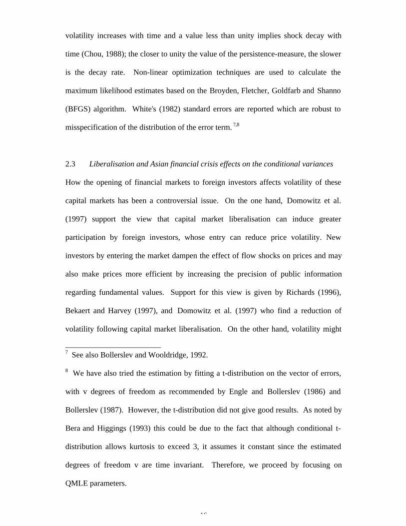
volatility increases with time and a value less than unity implies shock decay with

time (Chou, 1988); the closer to unity the value of the persistence-measure, the slower

is the decay rate. Non-linear optimization techniques are used to calculate the

maximum likelihood estimates based on the Broyden, Fletcher, Goldfarb and Shanno

(BFGS) algorithm. White's (1982) standard errors are reported which are robust to

misspecification of the distribution of the error term. 7,8

2.3 Liberalisation and Asian financial crisis effects on the conditional variances

How the opening of financial markets to foreign investors affects volatility of these

capital markets has been a controversial issue. On the one hand, Domowitz et al.

(1997) support the view that capital market liberalisation can induce greater

participation by foreign investors, whose entry can reduce price volatility. New

investors by entering the market dampen the effect of flow shocks on prices and may

also make prices more efficient by increasing the precision of public information

regarding fundamental values. Support for this view is given by Richards (1996),

Bekaert and Harvey (1997), and Domowitz et al. (1997) who find a reduction of

volatility following capital market liberalisation. On the other hand, volatility might

7 See also Bollerslev and Wooldridge, 1992.

8 We have also tried the estimation by fitting a t-distribution on the vector of errors,

with v degrees of freedom as recommended by Engle and Bollerslev (1986) and

Bollerslev (1987). However, the t-distribution did not give good results. As noted by

Bera and Higgings (1993) this could be due to the fact that although conditional t-

distribution allows kurtosis to exceed 3, it assumes it constant since the estimated

degrees of freedom v are time invariant. Therefore, we proceed by focusing on

QMLE parameters.

17

increase because of the increase in the amount of capital flows. Bekaert and Harvey

(2000) find a small but statistically insignificant increase in the volatility of stock

returns following liberalisation. Other studies, such as Kim and Singal (2000), find

no change in the volatility in the first two years of opening.

Looking now at exchange rate returns, theoretical analysis tells us that foreign

exchange controls reduce the volatility of exchange rates (see e.g. Phylaktis and

Wood, 1984). In addition, there is an argument supporting the view that shifts in

policy, such as a relaxation of foreign exchange restrictions, may have important

implications for the persistence of shocks to volatility,9 i.e. whether past volatility

explains current volatility. Because of this argument and the results of previous

studies, which generally indicate the existence of an effect of openness on the

volatility of local financial markets, we include a dummy variable on the conditional

variance of stock and foreign exchange returns, which assumes the value of one

before the official liberalisation date and zero otherwise and that is indicated with

DCi. Furthermore, we test whether the Asian financial crisis of mid 1997 had an

effect on the conditional variance of stock and exchange rate returns. Previous

studies, such as Schwert (1990), Engle and Mustafa (1992) Choudhry (1996) on the

financial crash of 1987, and of Choudhry (1995) on the great depression of 1929,

show that stock market volatility increased extensively after the crash or during a

crisis, but returned to pre-crash levels relatively quickly. Thus, in order to examine

the effects of the Asian financial crisis of mid 1997 on price volatility of Pacific Basin

countries’ equity and foreign exchange markets, we include another dummy variable,

(DUM) in the conditional variances of these two series, which assumes a value of one

9 See for instance Lastrapes, 1989 and Lamourex and Lastrapes, 1990.

18

from July 1997 to February 1998, and zero otherwise.10 The framework for the

conditional variances and covariances is modified as follows:

21,1

2111,

211

211, −− ++= ttiitii chbah ε + )1(1 ,

2tiDCD − + DUMDC 21

21,2

2221,

222

222

221, −− +++= ttxxtxx chbaah ε + )1(2 ,

2tiDCD − + DUMDC 22

21,3

2331,

233

233

232

231, −− ++++= ttmmtmm chbaaah ε

1,21,122111,22112111, −−− ++= tttixtix cchbbaah εε ,

1,31,133111,33113111, −−− ++= tttimtim cchbbaah εε

1t,31t,2133221t,xm332232223121t,xm cchbbaaaah −−− +++= εε . (14)

While this structure presents the advantage of recognizing the existence of

potential effects due to liberalisation and the Asian financial crisis on the conditional

volatilities of equity and foreign exchange returns, it does not allow the identification

of the sign. However, this framework allows the covariance matrix to be positive

definite without imposing any condition.

3. Capital market characteristics

3.1 Data

The sample of countries examined in the paper includes: Indonesia, Korea, Malaysia,

Philippines, Taiwan and Thailand. Hong Kong and Singapore have been excluded as

both countries had completely open capital markets since 1978, i.e. before the

beginning of our sample period. The data consist of end-of-month observations of

stock market index prices, and of local bilateral spot exchange rates expressed as units

10 The selection of this period is based on a previous study of Phylaktis and Ravazzolo

(1999), where considering the same countries, the authors identified that the Asian

crisis affected these economies for the above indicated period.

19

of U.S. dollar against one unit of each local Pacific Basin currency. The sample

covers monthly observations for the period 1980.01 to 2000.05 for Korea, Malaysia,

Taiwan and Thailand, and 1983:05 to 2000:05 and 1986:01 to 2000:05 for Indonesia

and Philippines respectively. All the data are from Datastream database.

3.1 Characteristics of stock and foreign exchange returns distribution

As a preliminary data analysis we applied the unit root testing methodology of

Philipps and Perron (1988) and failed to reject the null hypothesis of a unit root in the

logarithmic first difference of the price index of any of the time series under analysis.

The first difference of the stock price index and exchange rate of country i is

respectively defined as:

Ri,t = 100(logPi,t - logPi,t-1), (15)

Xi,t = 100(logSi,t - logS i, t-1), (16)

where Pi,t indicates the level of the stock prices for the index of country i, expressed in

local currency, and Si,t represents the bilateral spot exchange rate expressed as units of

U.S. dollar versus one unit of the local currency of country i.

Table 1 contains summary statistics for the data corresponding to stock and

foreign exchange returns. Not surprising, they have high means, which are associated

with high volatility. In particular, in most of the cases the standard deviation of stock

returns is higher than the standard deviation of foreign exchange returns. The most

volatile market is the Taiwanese one, which also presents one of the highest means

(see Panel A). In most of the cases the data corresponding to the time series of returns

on the stock and foreign exchange markets show skewness and high level of kurtosis.

The Bera-Jarque test statistic strongly rejects the hypothesis of normaly distributed

returns for all the markets under consideration.

20

Panel B in Table 1 reports autocorrelations for the returns in both stock and

foreign exchange markets. The predominant presence of autocorrelation in the return

series reveals that, in our analysis, we generally need to correct for autocorrelation in

the stock and currency markets induced by non-synchronous trading in the assets of

the financial markets as suggested by Lo and MacKinley (1988). Panel C in Table 1

contains the autocorrelation in the squared returns. The presence of statistically

significant autocorrelation in squared returns suggests that a GARCH

parameterisation for the second moments is required. The analysed market returns

present autocorrelation in their squared returns, with the exception of the Indonesian

and Philippines stock market returns, suggesting the use of conditional variance

processes in estimating second moments. As a result, we have excluded Indonesia

and Philippinnes from our sample.

3.2 Official liberalisation dates

In defining the dummy variable DCi, which takes a value of one before liberalization

and zero otherwise, we consider the official liberalization date as reported by the

International Finance Corporation (IFC). The IFC date is based on the Investibility

Index, which represents the ratio of the market capitalization of stocks that foreigners

can legally hold to total market capitalization. A large jump in the Index is evidence

of an official liberalization. The official liberalization date for the countries in our

sample is as follows: Korea, January 1992, when a new law was introduced allowing

foreign investors to own up to 10% of domestically listed firms; Malaysia, December

1988, when foreign investors were allowed to own up to 100% of domestic firms;

Taiwan, January 1991, when foreign investors were allowed to own up to 10% in any

of the domestic listed companies; and Thailand, September 1987. This date for

21

Thailand corresponds to the launch of the Alien Board in the Thai stock exchange,

where only securities available to foreign investors where traded. However,

international investors were still facing a foreign ownership limit of 49% and a lower

limit of 25% for commercial banks and finance companies.11

4. Empirical results

4.1 Conditional dynamic integration model on stock returns

We start our empirical analysis by estimating the conditional dynamic integration

model of De Santis and Imrohoroglu (1997) for the equity stock market returns of

Korea, Malaysia, Taiwan and Thailand, where the stock indices are expressed in local

currency (i.e. equations (3) and (11)). We take as a proxy for the world market

portfolio the U.S. stock market index. The findings are reported in Table 2. In

selecting the order of autoregressive components in the mean equation, we added lags

until the residuals did not present autocorrelation using the Ljung-Box statistic of

order twelve. We obtained that the order is one for Korea and Taiwan; four for

Malaysia and five for Thailand. In accordance with the results of De Santis and

Imrohoroglu (1997), the country-specific risk and the world market risk are not priced

for all countries, with the exception of Malaysia, where the estimated coefficients are

very small. The results also show that the conditional second moments are

appropriately described by the multivariate GARCH process. All the parameters in

matrices A, B, and C are statistically significant except 31α and 33c for Korea and 11α

11 For Thailand the IFC official liberalisation date is December 1988. However, as

noted by Bekaert and Harvey (2000), this date is not associated with any particular

regulatory changes. We do not present information for Indonesia and Philippines as

both of these countries were eventually left out from estimation.

22

for Thailand. The point estimates reveal that all the variance processes in Ht are

stationary and highly persistent. The Ljung-Box statistic tests of order twelve on the

standardized and squared standardized residuals show lack of autocorrelation and in

most cases the index of kurtosis for the standardized residuals is lower than the

corresponding index for the returns. However, it is still statistically significant

suggesting that the GARCH parameterization can accommodate part of the kurtosis in

the data.

Based on the obtained results, which show no relationship between expected

returns and market risks when estimating the dynamic integration model, we proceed

to re-estimate it by including the currency risk.

4.2 Conditional dynamic integration model with currency risk

The dynamic integration CAPM with currency risk relates to equations (7),

(10) and (11). The number of autoregressive components included in each of the

mean equations was selected as before through the use of the Ljung-Box statistic test

of order twelve.

In order to test whether volatility in our sample of countries changes over time

in a predictable fashion we estimate two versions of the model composed of the three

equations (7), (10) and (11). We refer to Model A when we assume constant

conditional variances and covariances, whereas we refer to Model B when we assume

that the conditional variances and covariances follow a GARCH(p,q) process. For

both models, we estimate the standardized residuals ( 2/1ˆˆˆ −= ttt huz ) and the squared

standardized residuals and then, for each series, we compute the Ljung-Box (LB)

statistic to test the null hypothesis of no autocorrelation up to order twelve. Overall,

the results in Table 3 support our specification.

23

Considering first the LB test statistic for the standardized residuals, the results

show that all market returns do not present residual autocorrelation, with the

exception of the Korean exchange rate, where the null hypothesis is rejected at the

10% level. The LB test for the squared standardized residuals shows that the

estimated statistics obtained from Model A have some form of autocorrelation. With

the exception of Taiwan, the autocorrelation disappears when the conditional

variances and covariances are assumed to follow a GARCH(p,q) process.

Finally, we perform the likelihood ratio statistic test on the estimated

unconditional and conditional processes, where we test for the null hypothesis that the

coefficients of the time varying variances and covariances of the conditional model

are equal to zero. In all the cases, the statistic tests reject the null hypothesis

indicating that the conditional structure outperforms the unconditional one.

Therefore, we use the parsimonious trivariate GARCH-in-Mean specification

presented in equation (13) to estimate the system composed of the expected equity

returns in local and U.S. markets and the currency returns as specified in equations

(7), (10), and (11).

The results of the trivariate conditional dynamic integration model inclusive of

currency risk are reported in Table 4.12 The following points can be made. First, the

results show that all GARCH parameters are highly significant. Secondly, the ci2 are

smaller than the bi2, which is an indication that lagged variances and covariances have

more weight than past innovations in explaining current variances and covariances.

This implies that large market surprises induce relatively small revisions in future

volatility. Third, the persistence of the conditional variance process, measured by bi2

12 We used the Akaike and the Schwarz information criteria to identify the best

performing GARCH(p,q) model.

24

+ ci2, is high and often close to the Integrated GARCH model of Engle and Bollerslev

(1986). According to Lamourex and Lastrapes (1990) the detected large persistence

may represent misspecification of the variances and result from structural change in

the unconditional variances of the process, as represented by changes in aia j in

equation (13). A discrete change in the unconditional variances of a process produces

clustering of large and small deviations, which may show up as persistence in a fitted

GARCH model. As previously discussed in Section 2.3, the liberalisation of the

financial markets under consideration and the Asian financial crisis of mid 1997 could

represent events, which might have caused a structural change in the unconditional

variances of the estimated process. Therefore, we re-estimate the system of equations

(7), (10) and (11) by fitting a GARCH process on their conditional variances and

covariances (equation (14)) that allows for the two structural changes in relation to

capital market liberalisation and the Asian financial crisis. The results are reported in

Table 5.

The evidence shows that in most of the cases there is a considerable reduction

in the persistence of the conditional variances in both stock and exchange market

returns. Secondly, the dummy variables for liberalisation and the Asian crisis are

highly statistically significant with the exception of the liberalisation dummy for the

currency returns in Taiwan and Thailand. In particular, the estimated coefficients

show that the effect of the Asian financial crisis is bigger than that of the liberalisation

on the volatility of the stock and currency returns of these markets. Moreover, we

identify a stronger effect on the financial markets of Thailand, followed by Korea and

Malaysia, while Taiwan is the country with the smallest effect. These effects

correspond to the strength of the crash in each of the countries. In general, these

findings show that there is an improvement in the specification of the modified model

25

when allowing for structural changes. In addition, even if the kurtosis of the

standardized residuals remains statistically different from zero and quite high for the

Thai currency returns, in almost all the cases there is a fall in the degree of

leptokurtosis from that reported in Table 1 for the raw data. This implies that the

model is correctly specified according to Hsieh (1989). Finally, the LB statistic tests

on both standardized and squared standardized residuals show absence of

autocorrelation and ARCH effect on the errors indicating the goodness of the fitted

GARCH process. As a result of the improved performance of the modified model, we

concentrate our discussion of the next two sections on the results obtained by it.

4.2.1 Equity markets

One of the major objectives of our analysis is to identify if the inclusion of the

currency risk improves the performance of the dynamic integration asset-pricing

model of De Santis and Imrohoroglu (1997) in pricing market risk. Our findings

show that the country-specific market risk is priced before liberalisation in all the

countries apart from Korea, while the world market risk is priced after liberalisation in

all the countries of our sample. The statistical significance of the coefficients

corresponding to the price of the world market risk suggests that all four Pacific Basin

capital markets are integrated after liberalisation. These findings are in accordance

with Bekaert and Harvey's (1995) results, who find also that these countries are

integrated with the world markets.13 However, we noted that the world market

13 One should be, however, cautious with Bekaert and Harvey’s results for two

reasons. First, their specification tests suggest that the model specification is rejected;

and secondly, according to the authors the estimation for Korea was extremely ill-

behaved and the model for Malaysia did not converge.

26

coefficients assume small values indicating that even if these countries are integrated,

there are still possibilities for obtaining portfolio diversification benefits.

An important result of our analysis is that the currency risk is found to affect

expected stock returns. Moreover, this risk is priced in both pre and post

liberalisation periods. This evidence is in accordance with previous studies of Dumas

and Solnik (1995) for US; De Santis and Gerald (1998) on the developed markets of

U.S., Japan, U.K. and Germany; and Carrieri (2001) on the European markets of

France, Germany, Italy, and U.K. In particular, the absolute value of the currency

price (see m13,i and m18,i in Table 5) is higher than the price of the market risk.14 The

estimated price of currency risk is negative in four of the six cases. According to

Dumas and Solnik (1995) the world price of currency risk should be negative when

the risk aversion of each investor sub-population is greater than one. In addition,

covariances are found to be statistically significant in ten out of twelve cases (see

m14,i, m16,i and m17,i in Table 5). Overall this evidence indicates that an international

asset-pricing model without exchange rate as a source of risk would be misspecified.

Therefore, the model used by De Santis and Imrohoroglu (1997) which does not

consider currency risk in pricing international assets might be misspecified.

The finding that currency risk affects stock market returns, particularly in the

pre-liberalisation period, is really interesting. This can be explained by the "flow"

channel discussed in Section 2.2, which links stock and foreign exchange market

14 Bailey et a. (2000) analysing the effect of association between stock and exchange

rate returns and variances on the Mexican financial markets during the peso crisis of

1994 noted that adverse exchange rate movements not only have an impact on

Mexican equity prices, but appear to lead many investors to rebalance their holdings

away from Mexico, causing a downward movement in the local equity returns.

27

movements, and can be related to economic integration found to be important for

financial integration even in the presence of capital restrictions (see Phylaktis and

Ravazzolo, 2002.

Focusing on the results for the world market return, which in our case is

represented by the U.S. stock returns, we find the estimated price for the world market

risk to be generally statistically significant (the only exception being Taiwan), but

small in magnitude. This evidence differs from the studies of De Santis and Gerard

(1997, 1998), Bekaert and Harvey (1995), De Santis and Imrohoroglu (1997), and

Harvey (1995). The previous findings show that the world market risk is not priced

when considering a model with constant world market price. For instance, De Santis

and Gerard (1997) obtained an estimated world price of 0.025 with statistical

significance of only 15 percent when considering the U.S. stock returns. However,

the different results might be related to the fact that with the exception of Bekaert and

Harvey (1995), all the mentioned studies estimated jointly the stock returns of all the

countries (including the world market returns) under the restriction that this parameter

is the same across different stock market returns.

4.2.2 Foreign exchange markets

The results for the currency returns show that there exists a statistically significant

relationship between currency risk and exchange rate returns in three out of four pre-

liberalisation cases (see coefficient m22,i in Table 5) and two out of the four post-

liberalisation cases (see coefficient m24,i in Table 5). In three of the above cases the

relationship is negative indicating that high volatility corresponds to a depreciation of

the local currency. As discussed in Section 2.2, this can be explained by the fact that

expectations of a depreciation of the local currency against the U.S. dollar, which can

28

be related to current account disequilibrium in pre-liberalisation period, and to both

current and capital account disequilibria in post liberalisation, may lead to speculative

attacks and to a fall in their value.

The results also show that in post liberalisation the price corresponding to the

covariance between the rate of appreciation and the world market returns (see

coefficient m25,i) is for all the countries a statistically significant component of

currency returns supporting the view that these markets are financially integrated.

Finally, the market price for the country-specific risk before liberalisation (see

coefficient m23,i) is significant for Korea, Taiwan and Thailand, but not for Malaysia.

This provides evidence that these stock and foreign exchange markets are also linked

in pre liberalisation period, through a "stock" and/or a "flow" channel.

4.2.3. The size of the risk premiums in equity markets

In this section, we present the market risk and exchange risk premiums and compare

their size and variance over different sub-periods and markets. Figures 1a – 1d

present plots of the total risk premium which is measured in the pre-liberalisation

period by

TRP = m12,ihii,t + m13,ihxx,t + m14,ihix,t (17)

and post-liberalisation period by

TRP = m15,ihim,t + m16,ihxm,t + m17,ihix,t + m18,ihxx,t. (18)

The first term in both expressions represents the market risk premium and the rest the

currency risk premium. The plots show in the case of Korea, Taiwan and Thailand

and perhaps less so in the case of Malaysia that risk premiums were considerably

29

more variable in the pre-liberalisation period compared to the post-liberalisation

period until the outbreak of the crisis in mid-1997.15

In Table 6, we report summary statistics for the total risk premium and its

decomposition into market and currency components. The statistics are given for the

full period and for the sub-periods identified by the plots. Namely, they are given for

the pre-liberalisation sub-period, the post-liberalisation until the crisis, the crisis

period until the end of the sample and the full sample period. The dates for the first

two sub-periods differ across countries since each one of them liberalised at different

times. Over the whole sample period, the annualised average value for the total

premium ranges from 2.09% for Taiwan, to 3.33% for Korea, to 7.32% for Thailand

and to –25.16% for Malaysia. The currency risk premium is substantial and forms a

big part of the total risk premium. In fact, in the case of Korea and Thailand, the

average value of the total risk premium is dominated by the value of the currency risk

premium, implying that the total premium from international investment is mostly a

reward for exposure to currency risk. In the case of the other two countries, the

currency risk premium is big and negative, and more than offsets the market risk

premium in the case of Malaysia, while it reduces the market risk premium from

14.51% to 2.09% in the case of Taiwan.

Looking however at the figures for the premiums for the various sub-periods,

one can see that the average figures for the whole sample period would have been

misleading as premiums varied substantially during the period. The currency risk

premium and total risk premium are bigger and more variable in the pre-liberalisation

period than in the post-liberalisation until the crisis, except for the case of Malaysia.

15 The rather quiet period in the early years in Taiwan and Thailand might reflect the

lack of development in these stock markets during that period.

30

In the post crisis period, the currency risk premium rises substantially across all

markets, is negative, and becomes also substantially variable. In the other sub-periods

no regularity concerning the sign of the currency risk premium is observed. The

premium takes positive and negative values.

5. Conclusion

In this paper, we have developed an international capital asset pricing model, which

included both market and currency risks and allowed full market segmentation until

the official liberalisation date and full integration thereafter. The dynamic integration

structure was also applied to pricing currency returns in accord with a risk adjusted

UIRP model. We used a parsimonious multivariate GARCH-in-Mean process in

estimating the conditional dynamics of our system of equations, which allowed also

for the examination of the effects of capital market liberalisation and the Asian

Financial crisis of mid 1997 on the volatilities of stock and currency returns.

Our main contribution is the incorporation of the currency risk in pricing

expected stock returns for markets whose degree of capital market integration

changes, which is a phenomenon of emerging markets. Consistent with Dumas and

Solnik (1995) and De Santis and Gerald (1998) we find strong support for the

specification of an ICAPM that includes both market and currency risk. Furthermore,

the risk is priced in both pre and post liberalisation periods. Thus, omitting foreign

currency risk in pricing international assets might give rise to model misspecafiction

as we have shown to be the case for De Santis and Imrohoroglu (1997). Bakaert and

Harvey (1995) attributed the rejection of the specification of their time-varying world

market integration model to the omission of currency risk too.

31

We also found that currency returns are related to their risk. In addition, we

noted that their covariance with the local stock market returns in pre-liberalisation and

with the world market returns in post-liberalisation are important explanatory factors.

Consistent with previous studies, such as Bekaert and Harvey (1995), our

results indicate that the Pacific Basin countries are integrated with world markets. In

particular, we noted integration also for countries such as Korea and Taiwan, which

maintained extensive capital controls during the 90s. These results have implications

for the use of foreign exchange restrictions to isolate capital markets from world

influences.

The empirical evidence reveals that the components of the risk premiums vary

significantly over time and across markets. The currency risk premium is substantial

and forms a big part of the total risk premium, dominating it at times. It is also bigger

and more variable when markets are segmented. In post Asian financial crisis period

it became negative across all markets and once again substantially variable.

Finally, our results show that market liberalisation and the Asian financial

crisis of mid 1997 affected the conditional variances of the stock and foreign

exchange returns. Unfortunately, our parameterisation did not allow us to infer the

direction of this effect. They highlight however the importance of taking into account

such structural changes when estimating international asset pricing models.

In general, our results have shown that currency risk is an important

component in international capital asset pricing models even during periods when

markets are not officially open to international investors. Since indeed currency risk

is priced and investors are compensated for bearing such risk they should not be

discouraged by more flexible exchange rate regimes from investing in emerging

markets.

32

Appendix A

Considering ρi the rate of return on security i, over a short holding period, expressed

in real terms (i.e. adjusted for inflation); the classic CAPM of Sharpe (1964) and

Lintner (1965) says that, in equilibrium, there must exist two numbers η and θ such

that

E(ρi ) = η + θcov(ρi,ρm ) (A.1)

where ρm represents the real rate of return on the market portfolio. The coefficient η

indicates the real riskless rate of return; and the coefficient θ can be interpreted as the

market average degree of risk aversion. The real rate of return is given as:

ρi = 11

R1

i

i −++

π, (A.2)

where Ri is the nominal rate of return of asset or market index i expressed in U.S.

dollar term, and iπ is the rate of inflation of country i expressed in U.S. dollar. Using

the Ito approximation and substituting equation (A.2) into equation (A.1), as in

Dumas (1994), we obtain

E(Ri) - E(πi) + var(πi) - cov(Ri, πi) = η + θcov(Ri - πi, Rm - πi) (A.3)

or rearranging the terms of equation (A.3),

E(Ri) = η + E(πi) - (1-θ)var(πi) - θcov(πi, Rm) + ( 1- θ)cov(Ri, πi) + θcov(Ri,Rm)

(A.4)

In equation (A.4) the first four terms of the right side of the equation sum to the

nominally riskless rate of return r. Hence, we can rewrite equation (A.4) as

E(Ri) = r + (1 - θ)cov(Ri,πi) + θcov(Ri,Rm). (A.5)

Equation (A.5) states that risky inflation produces a separate premium in nominal

returns. It is important to underline that the rate of inflation in any country may be

33

measured in any currency. For instance considering both the expected rate of return

on market index i and of inflation expressed in U.S. dollar, (A.5) becomes

E(Ri$) = r + (1 - θ)cov(Ri$,πi$) + θcov(Ri$,Rm), (A.6)

where E(Ri$) is the nominal rate of return of country i expressed in U.S dollar and πi$

is the rate of inflation of country i expressed in U.S. dollar. According to Solnik's case

the randomness of the rate of inflation of country i expressed in U.S. dollar is only

due to random fluctuation of the local currency of country i against the U.S. dollar.

Therefore, the term cov(Ri$,πi$) of equation (A.6) can be substituted by the covariance

between the rate of return on asset (or market index) i expressed in U.S. dollar units

and the rate of appreciation (depreciation) of the currency i respects to the U.S. dollar.

Therefore we can rewrite (A.6) as

E(Ri$) = r + (1 - θ)cov(Ri$,Xi$) + θcov(Ri$,Rm), (A.7)

with Xi$ the rate of appreciation of currency i against the U.S. dollar.

34

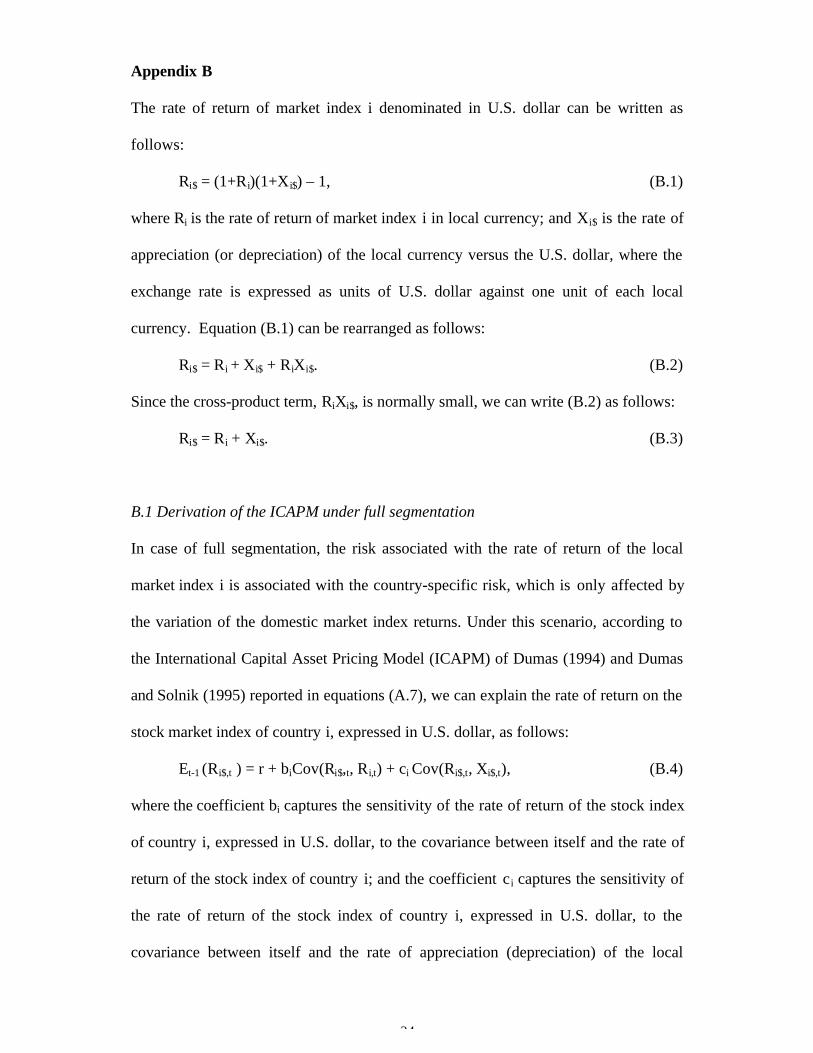
Appendix B

The rate of return of market index i denominated in U.S. dollar can be written as

follows:

Ri$ = (1+Ri)(1+Xi$) – 1, (B.1)

where Ri is the rate of return of market index i in local currency; and Xi$ is the rate of

appreciation (or depreciation) of the local currency versus the U.S. dollar, where the

exchange rate is expressed as units of U.S. dollar against one unit of each local

currency. Equation (B.1) can be rearranged as follows:

Ri$ = Ri + Xi$ + RiXi$. (B.2)

Since the cross-product term, RiXi$, is normally small, we can write (B.2) as follows:

Ri$ = Ri + Xi$. (B.3)

B.1 Derivation of the ICAPM under full segmentation

In case of full segmentation, the risk associated with the rate of return of the local

market index i is associated with the country-specific risk, which is only affected by

the variation of the domestic market index returns. Under this scenario, according to

the International Capital Asset Pricing Model (ICAPM) of Dumas (1994) and Dumas

and Solnik (1995) reported in equations (A.7), we can explain the rate of return on the

stock market index of country i, expressed in U.S. dollar, as follows:

Et-1 (Ri$,t ) = r + biCov(Ri$,t, Ri,t) + ci Cov(Ri$,t, Xi$,t), (B.4)

where the coefficient bi captures the sensitivity of the rate of return of the stock index

of country i, expressed in U.S. dollar, to the covariance between itself and the rate of

return of the stock index of country i; and the coefficient c i captures the sensitivity of

the rate of return of the stock index of country i, expressed in U.S. dollar, to the

covariance between itself and the rate of appreciation (depreciation) of the local

35

currency with respect to the U.S. dollar. bi and ci relate to the market’s risk aversion

and r is the riskless rate of return if there is one. Using (B.3) equation (B.4) can be

rearranged as follows:

Et-1 (Ri$,t ) = r + biCov(Ri,t+Xi$,t, Ri,t) + ciCov(Ri,t+Xi$,t, Xi$,t). (B.5)

Expanding the right hand side and noting that Cov(Xi$,t, Ri,t) appears twice, we write

(B.5) in a more general way amenable to empirical testing and using symbols

consistent with the ones in the rest of the paper as

Ri$, t= m10,i + kti

p

kik Rm −

=∑ $,

1,11 + m12,i hii,t + m13,ihxx,t+ 2m14,i hix, t + ε1,t,

( )t1tt,1 H,0N~I −ε (B.6)

where hii,t represents the conditional variance of the rate of return of the stock market

of country i, expressed in local currency; hix,t represents the conditional covariance

between the rate of return of the stock market index of country i and the rate of

appreciation (depreciation) of currency i; and hxx,t indicates the conditional variance

of the rate of appreciation (depreciation) of currency i.

B.2 Derivation of the ICAPM under full integration

As for the full segmentation scenario, we use the ICAPM of Dumas (1994) and

Dumas and Solnik (1995), which was introduced in equation (A.7), and explain the

rate of return on the stock index of country i, expressed in U.S. dollar as follows:

Et-1 (Ri$,t ) = r + biCov(Ri$,t, Rm,t) + ciCov(Ri$,t, Xi$,t), (B.7)

where the coefficient bi measures the sensitivity of the rate of return on the stock

index of country i, expressed in U.S. dollars, to its covariance with the market

portfolio rate of return; and the coefficient ci indicates the sensitivity of the rate of

return on the stock index of country i, expressed in U.S. dollar, to its covariance with

36

the rate of appreciation (depreciation) of the local currency. Using (B.3) equation

(B.7) can be rearranged as

Et-1 (Ri$,t ) = r + biCov(Ri,t+Xi$,t,Rm,t) + ciCov(Ri,t + Xi$,t, Xi$,t). (B.8)

Expanding the right-hand side and once again using a more general framework

and symbols consistent with the ones in the rest of the paper we write (B.8) as

Ri$,t = m10,i + kti

p

kik Rm −

=∑ $,

1,11 +m15,ihim,t +m16,ihxm,t + m17,i hix, t+m18,ihxx,t + ε1,t,

( )t1tt,1 H,0N~I −ε , (B.9)

where him,t represents the conditional covariance of the rate of return of the stock

market of country i, expressed in local currency and the market portfolio return; hmx,t

represents the conditional covariance between the rate of return of the market

portfolio and the rate of appreciation (depreciation) of currency i; hix,t represents the

conditional covariance of the rate of return of the stock market of country i, expressed

in local currency and the rate of appreciation of currency i; and hxx,t indicates the

conditional variance of the rate of appreciation (depreciation) of currency i.

B.3 The derivation of the rate of appreciation of the local currency

Dumas (1994) argues that if the financial market is integrated, the CAPM of equation

(A.5) applies to all securities. In fact equation (A.5) can be applied to explain the rate

of return from a foreign currency deposit, expressed in U.S. dollar as follows

ri = (1 + r*i)(1 + Xi$) - 1, (B.10)

where ri represents the rate of return on a currency deposit of country i, expressed in

U.S. dollar; r*i indicates the rate of return on a currency deposit of country i,

expressed in currency i; and Xi$ is the rate of appreciation (depreciation) of the

37

currency of country i with respect to the U.S. dollar. Equation (B.10) can be

rearranged as

ri = r*i + Xi$ + r*iXi$, (B.11)

where the term r*iXi$ is a really small number and therefore it can be rewritten as

follows

ri = r*i + Xi$. (B.12)

Thus, applying equation (A.5) to explain the rate of return on a foreign currency

deposit, expressed in U.S. dollars, we have

r*i,t + Et-1 (Xi$,t ) = ri,t + (1 - θ)cov(Xi$,t ,π) + θcov(Xi$,tRm,t), (B.13)

where r*i,t indicates the rate of return on a currency deposit of country i, expressed in

currency i; and Xi$,t is the rate of appreciation (depreciation) of the currency of

country i with respect to the U.S. dollar. This is a relationship between two short-

term nominal interest rates quoted in two different currencies or equivalently, between

the short-maturity forward premia and the expected spot exchange rate. Equation

(B.13) follows from viewing currency i's nominally riskless asset as a risky asset from

the viewpoint of a U.S. dollar investor, and noting that, according to Dumas (1994),

risks and required returns have the same equilibrium pricing structure, whether a risky

asset is a stock or a foreign currency deposit. Equation (B.13) provides the deviation

from the traditional UIRP, which prevails when investors are risk averse and PPP

does not hold. In equation (B.13) there exists equilibrium but the equilibrium

relationship between interest rates incorporates an inflation premium, which is a

deviation from nominal UIRP, and the reason being that investors care about real

returns. Equation (B.13) can be rearranged as follows

Et-1 (Xi$,t) = ri,t - r*i,t + (1 - θ)cov(Xi$,t ,π) + θcov(Xi$,t ,Rm,t). (B.14)

38

Assuming Solnik's special case as in Appendix A, where the rate of inflation

in country i is nonrandom, while the rate of inflation in country i measured in dollars

is random because of the randomness in the exchange rate, the term cov(Xi$,t π) is

equal to cov(Xi$,t, Xi$,t), which corresponds to var(Xi$,t), where the only random

component of inflation π is Xi$,t. Based on this assumption, we can rewrite equation

(B.14) as

Et-1 (Xi$,t ) = ri,t - r*i,t + (1 - θ)var(Xi$,t) + θcov(Xi$,t,Rm,t). (B.15)

Equation (B.15) represents the rate of appreciation of currency i in the case of

full integration. In the scenario of full segmentation, the component cov(Xi$,t,Rm,t) can

be substituted by the rate of return on the local stock market, expressed in domestic

currency, Ri, and it becomes

Et-1 (Xi$,t) = ri,t - r*i,t + (1 - θ) var(Xi$,t) + θcov(Xi$,t,Ri,t). (B.16)

Using the same symbols as for the stock market returns and assuming that the

interest rate differential is constant as there were no risk free interest rate data for our

emerging markets, the rate of appreciation of currency i in the scenario of full

segmentation is

Et-1 (Xi$,t )= m20,i + kti

p

kik Xm −

=∑ $,

1,21 + m22,ihxx,t + m23,ihix,t + ε2,t;

( )t1tt,2 H,0N~I −ε , (B.17)

where hxx represents the variance of the rate of appreciation of currency i, indicated as

Xi$; hix represents the covariance between the rate of appreciation of currency i and

the rate of return on the local stock market index of country i expressed in domestic

currency; and Ht is the conditional covariance matrix. Under the scenario of full

integration, equation (B.15) becomes

39

Xi$,t = m20,i + kti

p

kik Xm −

=∑ $,

1,21 + m24,ihxx,t + m25,ihmx,t + ε2,t, ( )t1tt,2 H,0N~I −ε ,

(B.18)

where hxm is the covariance between the rate of appreciation of currency i and the rate

of return of the world market portfolio.

40

References

Baba, Y., Engle, R.F., Kraft, D., Kroner, K.F., 1990. Multivariate simultaneous

generalised ARCH. Unpublished working paper. University of California, San Diego.

Bailey, W., Chan, K., Chung, Y.P., 2000. Depositary receipts, country funds, and the

Peso crash: the intraday evidence. Journal of Finance 55, 2693-2717.

Bekaert, G., Harvey, C.R., 1995. Time-varying world market integration. Journal of

Finance 50, 403-444.

Bekaert, G., Harvey, C.R., 1997. Emerging equity market volatility. Journal of

Financial Economics 43, 29-77.

Bekaert, G., Harvey, C.R., 2000. Foreign speculation and emerging equity markets.

Journal of Finance 55, 565-613.

Bekaert, G., Hodrick, R., 1992. Characterizing predictable components in excess

returns on equity and foreign exchange markets. Journal of Finance 47, 467-509.

Bera, A.K., Higgins, M.L., 1993. ARCH models: properties, estimation and testing.

Jouranl of Economic Surveys 4, 305-362.

Black, F., 1972. Capital market equilibrium with restricted borrowing. Journal of

Business 45, 444-455.

41

Bollerslev, T., 1987. A conditional heterosckedastic time series model for speculative

prices and rates of return. Review of Economics and Statistics 69, 542-547.

Bollerslev, T., Wooldridge, J.M., 1992. Quasi-maximum likelihood estimation and

inference in dynamic models with time-varying covariance. Econometric Reviews 11,

143-172.

Branson, W.H., 1983. Macroeconomic determinants of real exchange risk. In:

Herring, R.J., (Eds), Managing Foreign Exchange Risk. Cambridge University Press,

Cambridge, MA. pp. 33-74.

Campbell, J.Y., Hamao, Y., 1992. Predictable bonds and stock returns in the United

States and Japan: a study of long-term capital market integration. Journal of Finance

47, 43-70.

Carrieri, F., 2001. The effects of liberalisation on market and currency risk in the

European Union. European Financial Management 7, 259-290.

Chou, R., 1988. Volatility persistence and stock valuation: some empirical evidence

using GARCH. Journal of Applied Econometrics 3, 279-294.

Choudhry, T., 1995. Integrated-GARCH and non-stationary variance: evidence from

European stock markets during the 1920s and 1930s. Economics Letters 48, 55-59.

42

Choudhry, T., 1996. Stock market volatility and the crash of 1987: evidence from six

emerging markets. Journal of International Money and Finance 15, 969-981.

De Santis, G., Gerard, B., 1997. International asset pricing and portfolio

diversification with time-varying risk. Journal of Finance 52, 1881-1911.

De Santis, G., Gerard, G., 1998. How big is the premium for currency risk. Journal of

Financial Economics 48, 375-412.

De Santis, G., Imrohoroglu, S., 1997. Stock returns and volatility in emerging

financial markets. Journal of International Money and Finance 16, 561-579.

Domowitz, I., Glen, J., Madhavan, A., 1997. Market segmentation and stock prices:

evidence from an emerging market. Journal of Finance 52, 1059-1086.

Dornbusch, R., Fischer, S., 1980. Exchange rates and the current account. American

Economic Review 70, 960-971.

Dumas, B., 1994. A test of the international CAPM using business cycles indicators

as instrumental variables. In: Frankel, J. (Ed.), The Internationalisation of Equity

Markets. University of Chicago Press, Chicago, pp. 23-50.

Dumas, B., Solnik, B., 1995. The world price of foreign exchange risk. Journal of

Finance 50, 445-479.

43

Engle, R.F., Bollerslev, T., 1986. Modelling the persistence of conditional variances.

Econometric Reviews 5, 1-50.

Engle, R.F., Kroner, K.F., 1995. Multivariate simultaneous generalised ARCH.

Econometric Theory 11, 122-150.

Engle, R.F., Mustafa, C., 1992. Implied ARCH models from options prices. Journal of

Econometrics 52, 267-287.

Errunza, V.R., Losq, E., Padmanabhan, P., 1992. Tests of integration, mild

segmentation and segmentation hypotheses. Journal of Banking and Finance 16, 949-

972.

Ferson, W.E., Harvey, C.R., 1993. The risk and predictability of international equity

returns. Review of Financial Studies 6, 527-566.

Ferson, W.E., Harvey, C.R., 1994. Sources of risk and expected returns in global

equity markets. Journal of Banking and Finance 18, 775-803.

Frankel, J.A., 1983. Monetary and portfolio-balance models of exchange rate

determination. In: Bhandari J.S., Putnam, P.H., (Eds), Economic Interdependence and

Flexible Exchange Rates. MIT Press, Cambridge, MA. pp. 84-115.

Gavin, M., 1989. The stock market and exchange rate dynamics. Journal of

International Money and Finance 8, 181-200.

44

Glosten, L., Jagannathan R., Runkle, D., 1993. On the relation between the expected

value and the volatility of the nominal excess return on stocks. Journal of Finance 48,

1779-1801.

Grauer, F.L.A., Litzenberger, R.H., Stehle, R., 1976. Sharing rules and equilibrium in

an international capital market under uncertainty. Journal of Financial Economics 3,

233-256.

Harvey, C.R., 1991. The world price of covariance risk. Journal of Finance 46, 11-

157.

Harvey, C.R., 1995. Predictable risk and returns in emerging markets. Review of

Financial Studies 8, 773-816.

Hawawini, G., 1994. Equity price behaviour: some evidence from markets around the

World. Journal of Banking and Finance 18, 603-620.

Hsieh, D.A, 1989. Modelling heteroskedasticity in daily foreign exchange rates.

Journal of Business and Economic Statistics 7, 307-317.

Kim, E.H., Singal, V., 2000. Stock market openings: experience of emerging

economies. Journal of Business 73, 25-66.

45

Lamourex, C.G., Lastrapes, W.D., 1990. Persistence in variance, structural change,

and the GARCH model. Journal of Business and Economic Statistics 8, 225-234.

Lastrapes, W.D., 1989. Exchange rate volatility and US monetary policy: an ARCH

application. Journal of Money, Credit and Banking 21, 66-77.

Lintner, J., 1965. The valuation of risk assets and the selection of risky investments in

stock portfolios and capital budgets. Review of Economics and Statistics 47, 13-37.

Lo, A.W., MacKinley, A.C., 1988. Stock market prices do not follow random walks:

evidence from a simple specification test. The Review of Financial Studies 1, 41-66.

Phillips, P.C.B., Perron, P., 1988. Testing for unit root in time series regression.

Biometrica 75, 335-346.

Phylaktis, K., Ravazzolo, F., 1999. Stock prices and exchange rate dynamics.

Unpublished working paper. City University Business School.

Phylaktis, K., Ravazzolo, F., 2002. Measuring financial and economic integration

with equity prices in emerging markets. Journal of International, Money and Finance,

forthcoming.

Phylaktis, K., Wood, G.E., 1984. An analytical and taxonomic framework for the

study of exchange controls. In: Black J., Dorrance, G.S., (Eds), Problems of

International Finance. Macmillan, London, pp. 149-166.

46

Richards, A.J, 1996. Volatility and predictability in national stock markets: how

emerging and mature markets differ? IMF staff Papers 43, 461-501.

Schwert, G.W., 1990. Stock returns and real activity: a century of evidence. Journal of

Finance 45, 1237-1257.

Sharpe, W., 1964. Capital asset prices: a theory of market equilibrium under

conditions of risk. Journal of Finance 32, 493-502.

Solnik, B., 1974. An Equilibrium model of the international capital market. Journal of

Economic Theory. 8, 500-24.

Solnik, B., 1983. International arbitrage pricing theory. Journal of Finance, 38, 449-

457.

Wheatley, S, 1988. Some tests of international equity integration. Journal of Financial

Economics, 21, 177-212.

White, H., 1982. Maximum likelihood estimation of misspecification models.

Econometrica 50, 1-25.

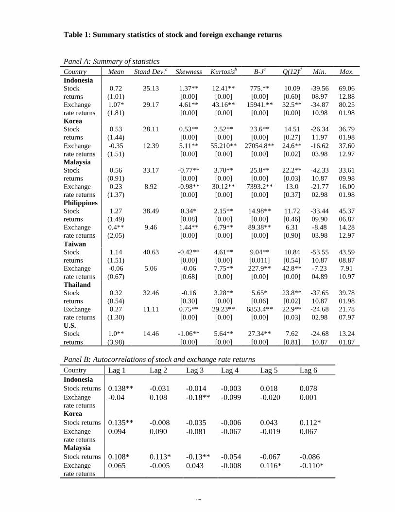
47

Table 1: Summary statistics of stock and foreign exchange returns

Panel A: Summary of statisticsCountry Mean Stand Dev.a Skewness Kurtosisb B-Jc Q(12)d Min. Max.IndonesiaStockreturns

0.72(1.01)

35.13 1.37**[0.00]

12.41**[0.00]

775.**[0.00]

10.09[0.60]

-39.5608.97

69.0612.88

Exchangerate returns

1.07*(1.81)

29.17 4.61**[0.00]

43.16**[0.00]

15941.**[0.00]

32.5**[0.00]

-34.8710.98

80.2501.98

KoreaStockreturns

0.53(1.44)

28.11 0.53**[0.00]

2.52**[0.00]

23.6**[0.00]

14.51[0.27]

-26.3411.97

36.7901.98

Exchangerate returns

-0.35(1.51)

12.39 5.11**[0.00]

55.210**[0.00]

27054.8**[0.00]

24.6**[0.02]

-16.6203.98

37.6012.97

MalaysiaStockreturns

0.56(0.91)

33.17 -0.77**[0.00]

3.70**[0.00]

25.8**[0.00]

22.2**[0.03]

-42.3310.87

33.6109.98

Exchangerate returns

0.23(1.37)

8.92 -0.98**[0.00]

30.12**[0.00]

7393.2**[0.00]

13.0[0.37]

-21.7702.98

16.0001.98

PhilippinesStockreturns

1.27(1.49)

38.49 0.34*[0.08]

2.15**[0.00]

14.98**[0.00]

11.72[0.46]

-33.4409.90

45.3706.87

Exchangerate returns

0.4**(2.05)

9.46 1.44**[0.00]

6.79**[0.00]

89.38**[0.00]

6.31[0.90]

-8.4803.98

14.2812.97

TaiwanStockreturns

1.14(1.51)

40.63 -0.42**[0.00]

4.61**[0.00]

9.04**[0.011]

10.84[0.54]

-53.5510.87

43.5908.87

Exchangerate returns

-0.06(0.67)

5.06 -0.06[0.68]

7.75**[0.00]

227.9**[0.00]

42.8**[0.00]

-7.2304.89

7.9110.97

ThailandStockreturns

0.32(0.54)

32.46 -0.16[0.30]

3.28**[0.00]

5.65*[0.06]

23.8**[0.02]

-37.6510.87

39.7801.98

Exchangerate returns

0.27(1.30)

11.11 0.75**[0.00]

29.23**[0.00]

6853.4**[0.00]

22.9**[0.03]

-24.6802.98

21.7807.97

U.S.Stockreturns

1.0**(3.98)

14.46 -1.06**[0.00]

5.64**[0.00]

27.34**[0.00]

7.62[0.81]

-24.6810.87

13.2401.87

Panel B: Autocorrelations of stock and exchange rate returnsCountry Lag 1 Lag 2 Lag 3 Lag 4 Lag 5 Lag 6IndonesiaStock returns 0.138** -0.031 -0.014 -0.003 0.018 0.078Exchangerate returns

-0.04 0.108 -0.18** -0.099 -0.020 0.001

KoreaStock returns 0.135** -0.008 -0.035 -0.006 0.043 0.112*Exchangerate returns

0.094 0.090 -0.081 -0.067 -0.019 0.067

MalaysiaStock returns 0.108* 0.113* -0.13** -0.054 -0.067 -0.086Exchangerate returns

0.065 -0.005 0.043 -0.008 0.116* -0.110*

48

PhilippinesStock returns 0.195** -0.017 -0.022 0.004 0.020 -0.019Exchangerate returns

0.019 0.091 0.000 0.111 0.015 0.032

TaiwanStock returns 0.055 -0.023 -0.056 0.051 0.029 -0.060ExchangeRate returns

0.124** 0.136** 0.170** -0.019 0.169** 0.159**

ThailandStock returns 0.124** 0.056 -0.032 -0.112* -0.130** 0.041Exchangerate returns

0.151** -0.094 0.023 -0.062 0.132** 0.063

U.S.Stock returns 0.008 -0.062 -0.063 -0.057 0.081 -0.032

Panel C: Autocorrelations of squared stock and exchange rate returnsCountry Lag 1 Lag 2 Lag 3 Lag 4 Lag 5 Lag 6IndonesiaStock returns 0.001 -0.006 0.032 0.021 0.032 -0.019Exchangerate returns

0.138** 0.013 0.034 0.189** 0.223** 0.034

KoreaStock returns 0.058 0.407** 0.161** 0.185** 0.137** 0.130**Exchangerate returns

0.287** 0.068 0.170** 0.054 0.021 0.003

MalaysiaStock returns 0.247** 0.080 0.235** 0.037 0.044 0.183**Exchangerate returns

0.464** 0.180** 0.083 0.221** 0.210** 0.199**

PhilippinesStock returns 0.087 0.074 0.039 0.000 0.094 0.046Exchangerate returns

0.160** 0.162** 0.335** 0.130* 0.148* 0.155**

TaiwanStock returns 0.353** 0.502** 0.319** 0.174** 0.205** 0.150**Exchangerate returns

0.148** 0.002 0.180** 0.200** 0.018 -0.019

ThailandStock returns 0.139** 0.158** 0.172** 0.181** 0.214** 0.097Exchangerate returns

0.334** 0.256** 0.097 0.077 0.201** 0.167**

U.S.Stock returns 0.060 0.050 0.008 0.032 -0.017 -0.003

Figures in parenthesis are t-statistics and in brackets p-values.a Each standard deviation is the monthly annualised one. This is computed by multiplying by12 the variance of the monthly data and taking the squared root of this value.bEqual to zero for the normal distribution.cBera-Jarque test statistic for normality.dLjung-Box test statistic of order 12.* and ** denote statistical significance at the 10% and 5% levels, respectively.

49

Table 2: Conditional dynamic integration model of stock returns

Quasi-maximum likelihood estimates of the model consisting of equations (3), (11) and the conditionalcovariance matrix given by (13) but excluding hxx,t, hix,t and hxm,t. The results are obtained using monthlyreturns from January 1980 to May 2000. L.F. indicates the maximum likelihood function. Figures inparenthesis are t-statistics and those in brackets are p-values. Estimates of constants and theautoregressive components in the mean equations are not presented.

Coefficients Korea Malaysia Taiwan Thailand

m12,I 0.003(0.567)

0.002**(177.0)

0.007(1.191)

0.005(0.107)

m15,I 0.005(0.029)

0.000**(12.50)

0.00(0.295)

0.00(0.044)

m32,I 0.002(0.584)

0.004**(288.30)

0.010(1.125)

0.002(0.215)

i,11α 1.640**(12.727)

-0.021**(-625.63)

-2.788**(4.781)

0.272(1.066)

i,31α 0.358(1.174)

0.012**(765.85)

-0.264*(-1.680)

0.354**(3.606)

i,33α -0.449**(-5.060)

-0.022**(-754.40)

-1.378**(-2.308)

0.222**(2.757)

b11,i 0.886**(120.46)

0.945**(56.70)

0.809**(9.883)

0.983**(3.304)

b33,i 0.987**(669.82)

0.872**(158.77)

0.920**(39.583)

0.993**(309.9)

i,11c 0.431**(49.33)

0.318**(13.03)

0.570**(3.153)

0.156**(4.943)

i,33c 0.070(1.574)

0.479**(15.47)

0.218**(4.262)

0.033**(2.480)

2i,11

2i,11 cb + 0.970 0.994 0.979 0.990

2i,33

2i,33 cb + 0.979 0.990 0.894 0.986

L.F. -1037 -1024 -1097 -1047Diagnosticstatistics forresiduals:

Korea US Malaysia US Taiwan US Thailand US

Skewness 0.30*[0.06]

-1.0**[0.00]

-0.52**[0.00]

-0.57**[0.00]

0.21[0.18]

-1.11**[0.00]

-0.73[0.0]

-1.10**[0.00]

Kurtosisa 1.06**[0.00]

6.**[0.00]

2.25**[0.00]

2.11**[0.00]

1.44**[0.00]

6.62**[0.00]

6.99**[0.00]

6.69**[0.00]

Q(12)b 11.4[0.49]

5.7[0.90]

16.28[0.18]

15.75[0.20]

8.80[0.72]

5.43[0.94]

8.83*[0.72]

6.11[0.91]

Q2(12)c 10.14[0.60]

9.52[0.70]

16.64[0.16]

6.62[0.88]

21.91**[0.03]

6.32[0.90]

11.25[0.51]

10.26[0.59]

a Equal to zero for the normal distribution.b & c Ljung-Box test statistic of order 12.* and ** denote statistical significance at the 10% and 5% levels, respectively.

50

Table 3: Specification tests

Country Q12(uh-1/2) Q12(uh-/12)2 Likelihoodratio test

Model A Model B Model A Model BKoreaStock returns 18.29

[0.11]18.07[0.11]

129.5**[0.00]

9.15[0.77]

692.0**[0.00]

Exchange rate returns 16.98[0.15]

21.37*[0.06]

75.41**[0.00]

18.59[0.10]

MalaysiaStock returns 18.50

[0.10]10.50[0.57]

99.43**[0.00]

7.60[0.82]

374.0**[0.00]

Exchange rate returns 15.99[0.19]

12.10[0.44]

65.72**[0.00]

15.30[0.23]

TaiwanStock returns 9.18

[0.69]9.28

[0.68]121.11**

[0.00]21.41**[0.04]

126.0**[0.00]

Exchamge ratereturns

19.09*[0.09]

17.99[0.12]

33.58**[0.00]

29.43**[0.00]

ThailandStock returns 15.38

[0.22]15.34[0.22]

68.05**[0.00]

13.43[0.34]

232.0**[0.00]

Exchange rate returns 18.16[0.11]

17.16[0.14]

80.51**[0.00]

3.11[0.99]

The first four columns contain Ljung-Box test statistics for the standardized residuals uh-1/2 and thesquared standardised residuals (uh-1/2)2. The statistics are computed for two models. Model Aasssumes a constant variance. Model B assumes a GARCH(p,q) process for the conditionalvariance. Both models assume a quasi-maximum likelihood distribution. The numbers in bracketsare p-values. The maximum order of auto-correlation is 12. The column labelled Likelihood ratiotest contains the likelihood ratio test statistics and correspondent p-values of the hypothesis ofconditional homoskedasticity. The test is distributed as a chi-squared with 8 degrees of freedom forKorea and 6 for the rest of the countries. * and ** denote statistical significance at the 10% and 5%levels, respectively.

51

Table 4: Conditional dynamic integration model inclusive of currency risk

Quasi-maximum likelihood estimates of the model consisting of equations (7), (10), (11) and the conditional covariancematrix given by (13). The results are obtained using monthly returns from January 1980 to May 2000. L.F. indicates themaximum likelihood function. Figures in parenthesis are t-statistics and those in brackets are p-values. Estimates ofconstants and the autoregressive components in the mean equations are not presented.

Coefficients Korea Malaysia Taiwan Thailandm12,I 0.001

(0.00)0.014**(2.919)

0.023**(2.713)

0.044**(2.735)

m13,i 0.000(0.580)

-0.547**(-2.604)

0.060**(3.184)

-0.225**(-6.789)

m14,i 3.013**(3.483)

-0.006**(-2.391)

-0.029**(-1.968)

0.007**(4.991)

m15,i 0.394**(2.119)

-0.000(-0.681)

0.002**(1.959)

0.003**(9.926)

m16,i 0.350**(3.449)

-0.028(-0.352)

0.044(0.123)

-0.015(-1.166)

m17,i 1.490(1.384)

0.000(0.378)

-0.096**(-3.261)

0.027**(9.967)

m18,i -0.384**(-5.724)

-0.012(-0.113)

1.579**(4.600)

-0.320**(-12.858)

m22,i -0.426**(-3.968)

0.002**(3.720)

-0.087(-1.458)

-0.147**(-3.487)

m13,I 0.212**(4.354)

0.061(1.404)

0.005*(1.700)

-0.154(-1.231)

m24,i -0.004(-0.433)

-0.012(-0.611)

-0.122**(-2.182)

0.007(1.305)

m25,i 0.956**(5.014)

0.000(0.141)

0.037(0.536)

-0.073**(-9.068)

m32,i 0.016**(1.909)

0.001(0.141)

0.004(0.682)

0.024**(3.405)

i,11α 1.273**(32.683)

2.122**(4.758)

2.351**(10.37)

0.034**(9.185)

i,21α 0.337**(25.428)

0.574**(186.43)

0.133**(4.97)

0.718**(5.632)

i,22α 0.008(0.174)

-0.628**(-4.169)

0.006(0.371)

0.961**(3.581)

i,31α 1.643**(27.07)

0.612**(3.673)

0.520**(4.206)

0.453**(3.092)

i,32α 0.338**(6.432)

0.213*(1.899)

0.018(1.056)

0.015(0.243)

i,33α -1.084**(-5. 647)

-0.566**(-3.654)

-1.050**(-5.873)

1.182**(6.115)

i,11b 0.869**(122.6)

0.858**(56.707)

0.905**(220.53)

0.947**(65.207)

i,22b 0.430**(53.94)

0.601**(20.832)

0.996**(14.49)

-0.375**(-3.595)

i,222b -0.078*(-1.646)

i,33b 0.855**(93.03)

0.953**(180.85)

0.938**(144.67)

0.929**(533.84)

i,11c 0.427**(81.173)

0.475**(8.719)

0.369**(32.13)

0.199**(32.56)

52

i,22c 0.420**(7.619)

0.644**(11.348)

0.036**(3.522)

0.520**(21.580)

i,222c 0.790**(100.73)

i,33c 0.150**(4.797)

0.222**(11.936)

0.216**(18.451)

0.184**(58.750)

2i,11

2i,11 cb + 0.937 0.962 0.953 0.936

2i,22

2i,22 cb + 0.991d 0.775 0.993 0.411

2i,33

2i,33 cb + 0.755 0.957 0.926 0.897

L.F. -1118 -1234 -1285 -1362Diagnosticstatistics forresiduals

Koreanstock

returns

Exchange rateretuns

U.S.stock

returns

Malaysianstock

returns

Exchange rate

rate

U.S.stock

returns

Taiwanesestock

returns

Exchange rate

rate

U.S.stock

returns

Thailandstock

returns

Exchange rate

rate

U.S.stock

returnsSkewness 0.22

[0.20]-0.5**[0.02]

-0.23[0.25]

-0.68**[0.00]

-1.07**[0.00]

-0.31[0.13]

0.18[0.27]

0.33[0.11]

-0.29[0.15]

-0.35**[0.02]

-5.29**[0.00]

-0.28[0.16]

Kurtosisa 1.23**[0.00]

3.04**[0.00]

0.79*[0.06]

2.36**[0.00]

5.84**[0.00]

0.77*[0.06]

1.53**[0.00]

6.71**[0.00]

0.80*[0.05]

2.98**[0.00]

48.25**[0.00]

0.80*[0.05]

Q(12)b 18.07[011]

21.37*[0.06]

6.04[0.90]

10.50[0.57]

12.10[0.44]

6.28[0.90]

9.28[0.68]

17.99[0.12]

6.10[0.91]

15.34[0.22]

17.16[0.14]

5.87[0.92]

Q2(12)c 9.15[0.77]

18.59[0.10]

10.2[0.59]

7.60[0.82]

15.30[0.23]

6.58[0.88]

21.41**[0.04]

29.43**[0.00]

6.41[0.89]

13.43[0.34]

3.11[0.99]

6.87[0.87]

aEqual to zero for the normal distribution.b & c Ljung-Box test statistic of order 12.dThis is the sum of 2

i,222

i,2222

i,22 c,b,b and 2i,222c .

* and ** denote statistical significance at the 10% and 5% levels, respectively.

53

Table 5: Conditional dynamic integration model inclusive of currency risk, and dummies for capitalmarket liberalisation and Asian crisis.

Quasi-maximum likelihood estimates of the model consisting of equations (7), (10) and (11) and the conditional covariancematrix given by (14). The results are obtained using monthly returns from January 1980 to May 2000. L.F. indicates themaximum likelihood function. Figures in parenthesis are t-statistics and those in brackets are p-values. Estimates ofconstants and the autoregressive components in the mean equations are not presented.

Coefficients

Korea Malaysia Taiwan Thailand

m12,i 0.000(0.011)

0.024**(2.577)

0.008**(1.925)

0.011*(1.650)

m13,i 0.837**(17.055)

-0.731(-1.091)

-0.059**(-6.547)

5.824**(11.195)

m14,i 0.049(0.719)

-0.037**(-3.306)

0.107**(-5.383)

-0.532**(-8.417)

m15,i 0.013**(10.005)

0.004**(16.595)

0.098**(2.138)

0.002**(3.017)

m16,i -1.021**(-16.345)

-0.011**(-4.843)

-0.045(0.728)

0.862**(7.267)

m17,i 0.007**(7.839)

0.008**(89.48)

-0.263**(-5.868)

-0.044**(-2.115)

m18,i -0.023**(-4.785)

-0.522**(-11.98)

-0.181**(-5.635)

0.045(0.538)

m22,i -1.482**(-15.06)

-0.110(-1.303)

-1.023**(-6.904)

0.447**(3.346)

m23,i 0.269**(25.113)

-0.003(-0.893)

0.431**(4.927)

-0.106**(-5.440)

m24,i -0.004(-0.370)

0.025**(5.124)

-0.063**(-2.408)

-0.017(-0.453)

m25,i 0.028**(3.918)

0.044**(38.916)

0.168**(2.068)

0.084**(14.978)

m32,i 0.086**(17.394)

0.001**(2.615)

0.004(0.552)

0.017**(19.792)

i,11α -2.275**(-9.182)

-0.791**(-35.756)

2.351**(3.250)

-2.167**(-7.269)

i,21α -0.082**(-2.912)

0.541**(64.987)

0.264**(5.350)

-1.076**(-31.299)

i,22α 0.357**(21.870)

0.594**(4.892)

-0.119**(-5.662)

-0.516*(-1.900)

i,31α 2.458**(19.503)

-1.003**(-9.269)

0.584**(5.816)

-1.432**(-4.966)

i,32α 0.128**(6.653)

-0.757**(-5.011)

0.116**(4.300)

1.058**(6.556)

i,33α 2.127**(10.634)

-1.103**(-10.797)

-0.924**(-5.856)

-0.817**(-2.288)

i,11b 0.760**(148.03)

0.883**(154.6)

0.852**(4.486)

0.780**(31.343)

i,22b 0.278**(36.550)

0.330**(99.90)

0.964**(3.654)

0.352**(4.562)

i,222b 0.603**(15.897)

-

i,33b 0.732** 0.899** 0.953** 0.797**

54

(69.869) (207.45) (3.400) (79.655)

i,11c 0.419**(173.783)

0.429**(177.57)

0.476**(39.090)

0.082**(10.638)

i,22c 0.032**(15.683)

0.257**(438.12)

0.027(0.877)

0.014**(2.570)

i,222c 0.475**(59.531)

-

i,33c 0.065**(2.941)

0.206**(75.12)

0.145**(9.305)

0.420**(33.281)

D1 0.130**(16.013)

0.727*(1.668)

-2.374*(-1.708)

5.177**(11.948)

D2 0.344**(2.046)

0.402**(27.67)

-0.005(-0.149)

0.009(0.221)

DC1 10.037**(4.216)

9.315**(25.99)

0.762(0.282)

11.288**(2.476)

DC2 10.773**(40.308)

4.942**(47.41)

-1.026**(-3.475)

11.864**(10.42)

2i,11

2i,11 cb + 0.753 0.964 0.951 0.615

2i,22

2i,22 cb + 0.665d 0.174 0.959 0.124

2i,33

2i,33 cb + 0.553 0.850 0.928 0.814

L.F. -1135 -1231 -1261 -1285Diagnosticstatistics forresiduals

KoreanStock

returns

Exchange rateretuns

U.S.stock

returns

Malaysianstock

returns

Exchange rate

rate

U.S.stock

returns

Taiwanese stockreturns

Exchange ratereturns

U.S.stock

returns

Thailandstock

returns

Exchange rate

rate

U.S.stock

returnsSkewness 0.59**

[0.00]-0.03[0.83]

-1.06**[0.00]

-0.35**[0.03]

-0.04[0.78]

-1.12**[0.00]

0.14[0.37]

0.56*[0.00]

-1.1**[0.00]

-0.47**[0.00]

-3.78**[0.00]

-1.51**[0.00]

Kurtosisa 0.72**[0.02]

1.28**[0.00]

6.01**[0.00]

1.56**[0.00]

2.01**[0.00]

6.50**[0.00]

1.19**[0.00]

6.30**[0.00]

6.43**[0.00]

2.94**[0.00]

36.2**[0.00]

9.6**[0.00]

Q(12)b 12.36[0.42]

15.54[0.21]

6.05[0.91]

10.56[0.57]

14.13[0.29]

6.11[0.91]

7.89[0.79]

11.12[0.51]

6.10[0.92]

6.68[0.88]

11.85[0.46]

7.05[0.85]

Q2(12)c 10.38[0.58]

16.21[0.18]

9.52[0.66]

5.70[0.93]

12.99[0.37]

6.43[0.89]

15.01[0.24]

7.42[0.83]

7.55[0.82]

8.89[0.71]

0.64[0.99]

3.97[0.98]

aEqual to zero for the normal distribution.b & c Ljung-Box test statistic of order 12.dThis is the sum of 2

i,222

i,2222

i,22 c,b,b and 2i,222c .

* and ** denote statistical significance at the 10% and 5% levels, respectively.

55

Table 6: Summary statistics for equity premiums

The table contains annualised means and standard deviations in brackets, in percent, for therisk premiums esimated for the dynamic integration model with currency risk and dummiesfor the Asian crisis and capital market liberalisation. The total risk premium (TRP) ismeasured as the sum of the market risk premium (MRP) and currency risk premium (CRP).The premiums for each stock market are measured in the pre-liberalisation period by

TRP = m12,ihii,t + m13,ihxx,t + m14,ihix,t and post-liberalisation period by

TRP = m15,ihim,t + m16,ihxm,t + m17,ihix,t + m18,ihxx,t.

Country TRP MRP CRPKorea Pre-liberalisation 80.01 - 91.12

30.72(273.94)

0.00(0.00)

30.72(273.94)

Post-liberalisation (excluding crisis) 92.01 - 97.06

-0.13(44.41)

0.09(3.68)

-0.23(45.38)

Post-crisis 97.06 - 00.-5

12.06(52.67)

17.46(6.75)

-5.42(50.42)

Full sample period 80.01 - 00.05

3.33(255.67)

0.93(5.56)

2.35(257.14)

Malaysia Pre-liberalisation 80.01 – 88.11

24.32(66.44)

24.66(64.14)

-1.55(9.34)

Post-liberalisation (excluding crisis) 88.11 - 97.06

-8.76(25.30)

0.41(1.12)

-9.08(25.13)

Post-crisis 97.06 - 00.-5

-433.92(374.0)

1.00(3.97)

-434.92(378.0)

Full sample period 80.01 - 00.05

-25.16(234.48)

11.49(44.07)

-36.66(228.67)

Taiwan Pre-liberalisation 80.01 - 90.12

10.11(64.47)

18.39(43.30)

-8.28(21.17)

Post-liberalisation (excluding crisis) 90.12 - 97.06

-1.76(45.52)

5.61(30.28)

-7.37(15.24)

Post-crisis 97.06 - 00.05

-19.53(68.4)

17.86(55.57)

-37.39(48.05)

Full sample period 80.01 - 00.05

2.09(66.99)

14.51(41.98)

-12.41(25.00)

Thailand Pre-liberalisation 80.01 - 87.08

24.96(75.24)

2.43(3.05)

22.56(74.88)

Post-liberalisation (excluding crisis) 87.09 - 97.06

-2.20(28.70)

0.42(2.22)

-2.62(29.96)

Post-crisis 97.06 - 00.05

-403.94(699.66)

2.69(1.04)

-406.63(699.56)

Full sample period 80.01 - 00.05

7.32(62.16)

1.32(3.06)

6.00(61.56)

56

Figure 1a

Figure 1b

Korean risk premium

-3,8

-1,8

0,2

2,2

4,2

6,2

Total risk premium Currency risk premium and CRMR

Malaysian risk premium

-14

-9

-4

1

6

Total risk premium Currency risk premium and CRMR

57

Figure 1c

Figure 1d

Thai risk premium

-10

-5

0

5

10

15

20

Total risk premium Currency risk premium and CRMR

Taiwanese risk premium

-40

-30

-20

-10

0

10

20

30

Total risk premium Currency risk premium and CRMR