Currency Carry, Momentum, and Global Interest Rate Uncertainty

Job Market Paper

Ming Zeng∗

November 13, 2018

ABSTRACT

Currency carry and momentum are among the most popular investment strategies in the foreign

exchange market. The carry (momentum) trade buys currencies with high-interest rates (recent

returns) and sells those with low-interest rates (recent returns). Both strategies are highly prof-

itable, but little is known on their common risk sources. This paper finds that their high returns are

compensations for the risk of global interest rate uncertainty (IRU), with risk exposures explaining

92% of their cross-sectional return variations. Profitability of two strategies also weakens substan-

tially when the global IRU risk is high. The unified explanation stems from its superior power

of capturing the crashes of carry and momentum, which usually occur during bad and good mar-

ket states. An intermediary-based exchange rate model confirms the negative price for the global

IRU risk. Higher uncertainty tightens intermediary’s financial constraints and triggers unwinding

on long and short positions. High (low) carry and momentum currencies then realize low (high)

returns as they are on the long (short) side of intermediary’s holdings. Further empirical evidence

indicates that the explanatory power for momentum extends to other asset classes, suggesting a

risk-based explanation for the commonality of momentum returns.

Keywords: Cross-section of carry and momentum; risk premium; uncertainty shocks; intermediary

asset pricing; momentum everywhere.

JEL Classification: E52, F31, G12, G15.

∗The author is with School of Economics, Singapore Management University. I thank Jun Yu and ThomasSargent for encouragement and continuous support. I am also grateful for comments from Pedro Barroso, PhilipDybvig, Dashan Huang, Huichou Huang, Junye Li, John Rogers, and seminar participants at Central University ofFinance and Economics, Fudan University, Nankai University, Peking University HSBC Business School, RenminUniversity of China, Singapore Management University, and University of Macau. All errors are my own. Emailaddress: ming.zeng.2013@smu.edu.sg.

1. Introduction

The foreign exchange (FX) market is the largest financial market in the world. The

triennial survey from the Bank for International Settlements (BIS) reports that the daily

FX trading volume is estimated to be $5.1 trillion as of 2016. The currency investment is

also very profitable. Among the most popular currency trading strategies, the cross-section

of carry and momentum trade yield average monthly excess returns of 0.58% and 0.51%

respectively, during the period from January 1985 to August 2017.1 As the FX market is very

liquid with low trading costs and easy access to the short-selling, a reasonable explanation for

the profitability is that their returns reflect risk compensations. However, little is known on

the common risk sources underlying these two types of trade, since the existing resolutions

based on the standard finance theory receive dismal performance empirically (see a review

by Burnside et al., 2011).

The main contribution of this paper is to provide a unified risk-based explanation for

the profitability of FX carry and momentum strategies. I find that the innovations to the

global interest rate uncertainty (IRU) are negatively and significantly correlated with the

returns to carry and momentum trade. To construct this global measure of uncertainty, I

first estimate the monthly realized variance of the government bond yields for each of the

G10 currencies. I show that the obtained interest rate uncertainty across different economies

strongly co-moves with each other, with the first principal component accounting for over

60% of their variations. The global IRU is then measured as the GDP-weighted average

over the individual uncertainty. After going through formal asset pricing tests by using the

innovations to the global IRU as the risk factor, I show that the exposures to the global IRU

risk can well explain the cross-sectional return dispersions of currency carry and momentum,

with the explanatory ratios reaching 89% and 97% respectively. More specifically, I find that

the top carry and momentum portfolios have lower and negative exposures (betas) to the

risk of global IRU , whereas their peers at the bottom have higher and positive betas. The

beta spreads are statistically significant and translate to negative and significant prices for

the global IRU risk. Considering the joint cross-section of carry and momentum returns

does not change the results. The cross-sectional R2 is 92% and the Shanken t-statistic for

the global IRU risk attains -2.8. Further exercises show that the main findings are robust

to different measures for the global IRU , such as those based on the realized volatility or

1These returns are from the viewpoint of a US investor and net of transaction costs. The cross-section of carry(momentum) trade buys the basket of currencies with the highest and shorts that with the lowest interest ratedifferentials (realized appreciations) against USD.

1

the US monetary policy uncertainty index of Baker et al. (2016).

To clarify economic channels behind the findings, using the aggregate stock return as

an indicator for market states, I show that periods when carry or momentum strategy ex-

periences exceptionally low returns correspond respectively to bad and good states for the

financial market. Remarkably, these periods are accompanied by large innovations to the

global IRU . Thus it is the ability of global IRU shocks to capture both bad and good market

states that renders the joint explanatory power for currency carry and momentum. While

the role of uncertainty as a barometer for the bad states is easier to digest following a large

strand of literature (see, e.g., Bloom, 2009; Brogaard and Detzel, 2015), it is less obvious

why sometimes higher IRU can indicate good states for the financial market. Nevertheless,

this might not be so surprising as Segal et al. (2015) document that the fluctuating growth

uncertainty contains two components that are associated with positive or negative shocks to

the economy. I show empirically that the innovations to the global IRU indeed provide a

comprehensive measure over good and bad states for the economy and the financial markets.

The formal theoretical analysis based on a structural exchange rate model confirms that

the innovations to the global IRU is a pervasive risk factor in the pricing kernel and carry

a negative price of risk. The model follows the spirit of Gabaix and Maggiori (2015) and

Mueller et al. (2017b) by highlighting the role of sophisticated financial intermediary as the

marginal investor in the currency market. Higher global interest rate uncertainty increases

the shadow price of intermediary’s financial constraints and hence drives up the marginal

utility of the intermediary. This renders a negative price for the global IRU risk among

currency carry and momentum returns. More precisely, currencies with high (low) carry or

momentum signals are on the long (short) side of intermediary’s holdings in equilibrium.

The reason is that higher interest rates push up intermediary’s investment yields, whereas

higher appreciations predict lower selling pressures by international investors in the future

so that the intermediary would find them more attractive to hold today. Rising global

IRU leads to position unwinding by the intermediary, but currencies with high or low carry

(momentum) signals respond differently since one currency tends to depreciate (appreciate)

when the intermediary holds (short-sells) less of it. Therefore, the theory is consistent with

the documented negative correlations between the global IRU risk and returns to carry and

momentum trade.

Further in line with the intermediary-based story, the explanatory power of the global

IRU risk also presents for momentum in other asset classes. I find that the impact of the

global IRU risk is quantitatively large among momentum in seven asset classes as discussed

2

by Asness et al. (2013), in addition to the currency momentum. Almost all momentum

strategies realize sizable losses when the global IRU risk becomes higher. For example,

one standard deviation change of the global IRU risk is associated with a -0.39% (-0.48%)

monthly loss of the momentum trade in US (UK) equity markets. The effect is similar

and statistically significant for most markets. While Asness et al. (2013) employs the story

of funding liquidity risk as a resolution for the commonality of momentum returns across

asset classes, I show that the explanatory power of the global IRU risk is comparably

much stronger in terms of both economic magnitudes and statistical significance. The cross-

sectional asset pricing tests indicate that the high-minus-low spreads in IRU betas among

momentum portfolios are negative and significant for most of the asset classes. The estimated

risk prices from all momentum portfolios attain the same sign and significance compared with

that from the FX market. Remarkably, the standard CAPM model augmented with the

factor of global IRU risk even yields similar explanatory ratio on cross-sectional momentum

returns, compared with the model consisting of the global momentum factor as proposed by

Asness et al. (2013).

The unified explanations on currency carry and momentum based on the global IRU

risk factor is attractive. First, it is a variable constructed outside the FX market, yet

many competing factors are currency-based measures of systematic risk (see, e.g., Lustig

et al., 2011; Corte et al., 2016). Thus the global IRU risk is unlikely to be mechanically

related to the testing currency portfolios. Moreover, the time-varying domestic interest rate

uncertainty should be largely exogenous to the FX market fluctuations, especially for G10

currencies that belong to the developed economies. Essentially, it is not surprising that the

model based on the global interest rate uncertainty performs so well, given the critical role

of monetary policy on affecting the currency markets. While the level of interest rate may

matter more when explaining domestic financial markets (e.g. Maio and Santa-Clara, 2017),

it is obvious that increased rate of one country can have the very limited impact on the

cross-section of currency strategies. In contrast, the interest rate uncertainty, which displays

strong co-movements across different countries, is more suitable for obtaining the global risk

factor that governs the currency risk premia.

To corroborate the main findings, I carry out a battery of robustness checks. First, the

results are invariant to using different testing procedures such as the Fama-MacBeth regres-

sion or the GMM estimation. The results are even stronger if using the factor-mimicking

portfolio return as the risk factor in the test. Second, after controlling for other risk factors

and measures of financial frictions, I find that the unified pricing power of the global IRU

3

risk on FX carry and momentum returns is not affected. The performance is also robust un-

der different limits to arbitrage measured by the idiosyncratic volatility or skewness. Third,

the currency-level study alike points to a negative and significant price of the global IRU

risk. In particular, high-interest rate currencies such as the Australian Dollar (AUD) and

the New Zealand Dollar (NZD) indeed have low and negative IRU betas, as opposed to

low-interest rate currencies such as the Japanese Yen (JPY) and the Swiss Francs (CHF).

Last but not least, the asset pricing results are robust under different subsamples covering

e.g., the pre- and post-crisis periods or the developed economies.

Related literature The paper contributes to a large strand of literature towards under-

standing the risk sources of high returns to currency strategies. Most of the previous papers

focus on the cross-section of the carry trade. Lustig and Verdelhan (2007) interpret its

returns as exposures to the risk of consumption growth, and Lustig et al. (2011) further

reconcile its profitability via the slope factor constructed from the carry trade portfolios.

Based on the ICAPM argument, Menkhoff et al. (2012a) find that changes in the global FX

volatility help explain the carry returns. Among other resolutions, Burnside et al. (2010)

argue that the carry trade returns reflect a peso problem, whereas Lettau et al. (2014) and

Dobrynskaya (2014) highlight the importance of downside risk. The more recent focus has

been switched to understand the currency momentum. Burnside et al. (2011) and Menkhof-

f et al. (2012b) find that the correlation between carry and momentum returns is small,

and traditional risk factors cannot explain the cross-section of momentum returns. Filippou

et al. (2018) show that the global political risk can reconcile the momentum returns. Bae

and Elkamhi (2017) further price the joint cross-section of carry and momentum by the risk

of global equity correlation. My paper is tightly linked with all these articles. I show em-

pirically that the risk of global interest rate uncertainty can explain the returns to currency

carry and momentum strategies. The unified risk-based resolution is robust and unrelated to

existing risk factors. The explanatory power is consistent with an intermediary-based asset

pricing model and stems from its unique role of capturing the downturns of both strategies.

An attractive feature of my resolution besides its strong performance is that the interest rate

uncertainty measured directly from government bond yields is likely to be exogenous to the

FX markets, compared with many competing risk factors.

This article is also related to the recent literature on studying the asset pricing implica-

tions of policy uncertainty. Besides the theoretical framework of Pastor and Veronesi (2012)

and Pastor and Veronesi (2013), Brogaard and Detzel (2015) empirically evaluate the pric-

ing of policy uncertainty in the stock market via the Economic Policy Uncertainty index of

4

Baker et al. (2016). Nevertheless, the discussion within the FX market is still at the infant

stage, with some exceptions including, e.g., Berg and Mark (2017). In particular, my paper

is closely related to Mueller et al. (2017b), who find that the profitability of the carry trade

and the strategy that buys foreign currencies and short-sells the USD is significantly higher

during the FOMC announcements. While they study the high-frequency behavior of these

currency returns and interpret the results as compensations for the risk of US monetary

policy uncertainty, my paper differs from theirs in two important perspectives. First, my

paper follows more standard asset pricing test by examining and reconciling the well-known

currency risk premium anomalies at the monthly frequency. Moreover, they do not study

the currency momentum and further the unified risk-based explanation for the FX carry and

momentum returns. I thus treat the conclusions from my paper as important complements

to theirs in the sense that we both highlight the value of monetary policy uncertainty in

understanding the currency risk premium, at both high- and low-frequency.

The paper is organized as follows. Section 2 describes the data and methodology. Section

3 documents the main empirical results. Section 4 discusses the economic channels behind

the novel findings. Section 5 includes a battery of robustness checks, and Section 6 concludes.

2. Data and Methodology

2.1. Currency carry and momentum portfolios

The data for the spot exchange rates and one-month forward rates cover 48 countries

and range from January 1985 to August 2017. The data are from the Datastream (Barclays

Bank International and Reuters). I remove the Eurozone currencies after the adoption of

Euro, and also remove the periods for some currencies when there are violations in the

Covered Interest Rate Parities (CIP). To form the carry and momentum portfolios, I use the

information from mid-level spot and forward rates, but the portfolio returns are computed

by taking into account the bid-ask spreads, following e.g., Menkhoff et al. (2012b).2

Denote the mid-spot rate as St which represents units of foreign currency per unit of

US dollar, and denote the one-month mid-forward rate as Ft. As the proxy for the interest

rate differential between the foreign country and the US, I follow the literature by using the

2Details are given in the Data Appendix. The bid-ask data are also available from Reuters, and in the InternetAppendix I show how to account for transaction costs when computing portfolio returns. Note that the bid-askspread data from Reuters are around twice the size of inter-dealer spreads, as documented by Lyons (2001).

5

forward discount (e.g., Lustig et al., 2011):

i∗t − it ≈ ft − st, (1)

where the small letters stand for log terms. Then the one-period log currency excess return

rxt+1 can be computed as:

rxt+1 = i∗t − it −∆st+1 ≈ ft − st+1. (2)

To form the carry trade portfolios, I first sort on all currencies’ forward discounts at the

end of each month. Then each currency is attributed to one of the quintile portfolios, where

portfolio 1 (5) consists of currencies with the lowest (highest) interest rate differentials vis-a-

vis the United States. To construct the momentum trade portfolios, I sort on currencies’ past

realized excess returns at the end of each month, where the realized quantities are computed

over the past 3-month horizons.3 Then five portfolios are formed, where the portfolio 1 (5)

contains currencies with lowest (highest) realized excess returns. They are also called the

loser and the winner portfolio respectively. All portfolios are rebalanced monthly, and their

excess returns are computed via the equal-weighted scheme.

The first column of each panel in Table 1 reports the average monthly excess returns

of carry and momentum portfolios, after taking into account the bid-ask spreads. In line

with the findings in the literature, the strategy profitability is large and significant. The

average monthly high-minus-low return spreads for the carry and momentum portfolios are

0.58% and 0.51%. Furthermore, the returns increase monotonically from the bottom to

the top portfolios, revealing the substantial predictive power of interest rate differentials

and realized currency returns on future returns. The monotonic order is also supported

statistically by the test of monotonic relations (MR) following Patton and Timmermann

(2010). I report in parentheses the p-values of testing the null hypothesis that the portfolio

returns are monotonically increasing, which are based on all pair-wise comparisons. The null

hypothesis cannot be rejected at any conventional confidence levels.

[Table 1 about here]

3I provide robustness checks for other horizons in the Internet Appendix.

6

2.2. Measuring global interest rate uncertainty

I focus on the universe of G10 currencies to construct the global measure as they play

dominant roles in the FX markets. To estimate the interest rate uncertainty (IRU) for

each individual currency, I rely on their daily government bond yields to obtain the monthly

interest rate realized variance, similar to Cieslak and Povala (2016). The data of US 10-year

bond yields are from FRED and those of other currencies are from Bloomberg.4 Panel A of

Table 2 tabulates the correlation matrix of the individual interest rate uncertainty. The large

correlation coefficients point to a strong factor structure among these uncertainty measures.

Indeed, the displayed outputs from the Principal Component Analysis (PCA) in Panel B

show that the first principal component explains around 60%, and the first three components

in total explain around 80% of the variations in the interest rate uncertainty during the entire

sample. Splitting into pre- and post-crisis samples yields quite similar results, suggesting

that the factor structure is not due to the presence of 2008 global financial crisis. To account

for the potentially different impact of each currency’s interest rate uncertainty on the global

financial market, I adopt the GDP-weighted average over all individual IRU as the baseline

measure for the global (IRU).5

[Table 2 about here]

[Figure 1 about here]

The upper panel of Figure 1 plots the level of estimated global IRU from January 1985

to August 2017, and the lower panel depicts the standardized innovations (uIRUt ) obtained

as the residuals from fitting an AR(1) model to the level series. The global interest rate

uncertainty does indeed capture important periods corresponding to sharp changes in the

international financial markets, such as the Black Monday, collapse of Long-Term Capital

Management (LTCM), recent global financial crisis, and Euro-debt crisis etc. Table 3 then

reports the correlation coefficients of uIRUt with the returns to currency carry, momentum,

and conventional risk factors. The results are consistent with usual findings in the literature

4The focus on 10-year maturity is mainly due to the data availability issue as the data on other maturities arecomparably shorter for many countries. The G10 currencies cover United States dollar (USD), Euro (EUR), Poundsterling (GBP), Japanese yen (JPY), Australian dollar (AUD), New Zealand dollar (NZD), Canadian dollar (CAD),Swiss franc (CHF), Norwegian krone (NOK) and Swedish krona (SEK). In particular, I use Germany 10-year bondyields as the interest rates for the Euro. The details of data availability for each economy is in the Data Appendix.

5The weights are each country’s world share of GDP based on the purchasing-power-parity (PPP), with the datafrom IMF database.

7

that returns to these two currency strategies are weakly correlated with popular risk factors

(e.g. Burnside et al., 2011). In fact, the correlation between carry and momentum returns is

close to zero, further highlighting the difficulty of establishing a unified explanation. In spite

of the fact that the carry returns are significantly related with the risk of consumption growth,

VIX or global FX volatility (see, e.g., Lustig and Verdelhan, 2007; Brunnermeier et al.,

2008; Menkhoff et al., 2012a), none of them are significantly correlated with the momentum

returns. Interestingly, the innovations in the global IRU are strongly and negatively related

with both strategy returns at the 1% significance level. The negative correlations suggest

that both carry and momentum returns should drop when innovations to the global IRU

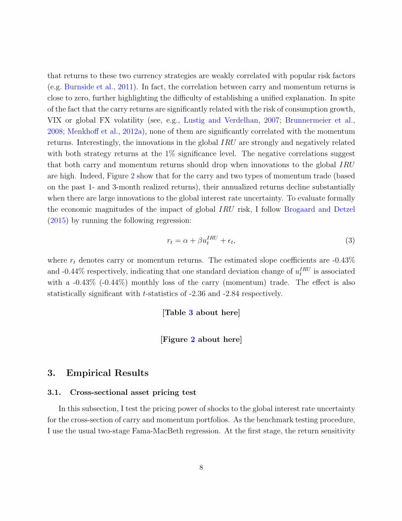
are high. Indeed, Figure 2 show that for the carry and two types of momentum trade (based

on the past 1- and 3-month realized returns), their annualized returns decline substantially

when there are large innovations to the global interest rate uncertainty. To evaluate formally

the economic magnitudes of the impact of global IRU risk, I follow Brogaard and Detzel

(2015) by running the following regression:

rt = α + βuIRUt + εt, (3)

where rt denotes carry or momentum returns. The estimated slope coefficients are -0.43%

and -0.44% respectively, indicating that one standard deviation change of uIRUt is associated

with a -0.43% (-0.44%) monthly loss of the carry (momentum) trade. The effect is also

statistically significant with t-statistics of -2.36 and -2.84 respectively.

[Table 3 about here]

[Figure 2 about here]

3. Empirical Results

3.1. Cross-sectional asset pricing test

In this subsection, I test the pricing power of shocks to the global interest rate uncertainty

for the cross-section of carry and momentum portfolios. As the benchmark testing procedure,

I use the usual two-stage Fama-MacBeth regression. At the first stage, the return sensitivity

8

to the global IRU shocks for each portfolio i is estimated from the time-series regression:

rxit = αi + βiDOLDOLt + βi

IRUuIRUt + εit, (4)

where DOLt is the dollar factor constructed as the cross-sectional average of excess returns of

five carry trade portfolios following Lustig et al. (2011). It can be treated analogously as the

market factor in the FX market. Then at the second stage, I run the following cross-sectional

regression:

rxi = βiDOLλDOL + βi

IRUλIRU + ηi, (5)

where the left-hand side is the unconditional mean of portfolio excess returns, and the first-

stage estimated betas are used as the explanatory variables on the right-hand side. λDOL

and λIRU are the risk prices per unit of dollar factor beta and IRU beta. Note that I do

not add the intercept at the second stage regression due to the inclusion of the dollar factor

(see, e.g., Menkhoff et al., 2012a).

The rest columns of Table 1 report the outcomes of first-stage time-series regression, where

the standard errors of estimated betas are based on Newey and West (1987) with optimal lag

selection following Andrews (1991). For both types of cross-sectional portfolios, while they

load similarly on the dollar factor, their exposures to uIRUt decrease almost monotonically

from the bottom to the top portfolios. The patterns are also plotted in the upper panel

of Figure 3. In fact, the magnitudes of high-minus-low beta spreads are similar and also

statistically significant at the 5% level. Obtaining a significant spread in betas is a pivotal

check on whether the factor is priced following Kan and Zhang (1999) and Burnside (2011).

The monotonic relations are statistically justified via the monotonicity test on betas following

Patton and Timmermann (2010), where the p-values are reported and based on the null

hypothesis that the betas are monotonically decreasing. The first-stage evidence hence sheds

light on the potentially unified explanation of the currency carry and momentum returns by

their exposures to the risk of global IRU .

[Figure 3 about here]

After obtaining the betas, the cross-sectional regression (5) is estimated via OLS. For

test on the statistical significance of risk prices, I employ the heteroskedastic and autocor-

relation consistent (HAC) standard errors based on Newey and West (1987) with optimal

lag selection following Andrews (1991) (NW), as well as those of Shanken (1992) (Sh) that

9

further incorporate the adjustments due to the error-in-variable (EIV) problem of using first-

stage estimated betas. To recognize the specific and unified pricing power, I use five carry

and five momentum portfolios separately or jointly as testing assets. Panel A of Table 4

documents the results. The almost monotonically decreasing betas and increasing portfolio

returns render the negative prices for the global IRU risk, with the cross-sectional R2 of

89% and 97% respectively. The large R2 indicates that exposures to IRU risk go a long

way towards reconciling the returns to FX carry and momentum trade. Meanwhile, the

magnitudes of risk prices are similar and significant under both types of standard errors.

The results are invariant for the joint cross-section of carry and momentum returns, with

the R2 of 92%. To test for zero pricing errors, I further report the p-values from the χ2-test

as discussed in e.g., Cochrane (2005). The computation of χ2 statistics are also based on the

method of Newey-West (χ2NW ) or Shanken (χ2

Sh). From the table, the null hypothesis that

all pricing errors are jointly zero cannot be rejected when separately using the carry and

momentum portfolios as testing assets. This indicates close distance between the average

portfolio returns and the fitted returns from Equation (5), as can be found from the lower

panel of Figure 3.

[Table 4 about here]

However, the global IRU risk is a non-traded factor. To mitigate the concern of using

such type of factor in the asset pricing test, as widely discussed in e.g., Kan and Zhang (1999),

I construct the factor-mimicking portfolio by projecting uIRUt on ten currency portfolios:

uIRUt = a+ b′wt + εt, (6)

where wt denotes the vector of month-t excess returns of five carry and five momentum port-

folios. The correlation coefficient between the obtained factor-mimicking portfolio returns

and uIRUt is 0.26. Since uIRU

FMM,t is now a traded factor, without going through any asset

pricing test, the Sharpe ratio of the factor-mimicking portfolio already reflects the market

price of IRU risk. Its monthly SR is -0.27 with a Newey-West t-statistic of -4.81. The mag-

nitude of SR is even slightly larger than those of carry and momentum strategies, suggesting

that the global IRU risk explains a bulk of the strategy returns. Then I follow the previous

exercises by running the cross-sectional asset pricing test, using uIRUFMM,t instead of uIRU

t as

the risk factor. The results are in Panel B of Table 4. The main findings are still there

with large cross-sectional R2, but now the risk prices become more significant, thanks to

10

the usage of traded risk factor in the test that yields more accurate inference. The Shanken

t-statistic reach as large as -5.0 when using the joint cross-section of currency portfolios as

testing assets.

The two-stage method though is easy to implement, the pre-estimation of IRU betas

is unfavorable because it introduces the error-in-variable problem when running the cross-

sectional test. I thereby employ the Generalized Method of Moments (GMM) to estimate

the asset pricing model in one-step directly. The analysis begins with a parametric form for

the stochastic discount factor (SDF) that is linear in risk factors:

Mt+1 = 1− bDOL(DOLt+1 − µDOL)− bIRUuIRUt+1 , (7)

and the Euler equations:

E(Mt+1RXit+1) = 0, (8)

where RX it+1 is the excess return of testing asset i. Denote ht = [DOLt−µDOL, u

IRUt ]′, then

I set up the moment conditions as follows:

E(gt+1) = E

(1− bDOL(DOLt+1 − µDOL)− bIRUuIRUt+1 )RX i

t+1

DOLt+1 − µDOL

ht+1h′t+1 − ΣDOL,IRU

= 0. (9)

These moment conditions allow for the joint inference on the parameters of SDF and risk

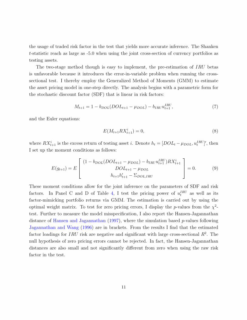
factors. In Panel C and D of Table 4, I test the pricing power of uIRUt as well as its

factor-mimicking portfolio returns via GMM. The estimation is carried out by using the

optimal weight matrix. To test for zero pricing errors, I display the p-values from the χ2-

test. Further to measure the model misspecification, I also report the Hansen-Jagannathan

distance of Hansen and Jagannathan (1997), where the simulation based p-values following

Jagannathan and Wang (1996) are in brackets. From the results I find that the estimated

factor loadings for IRU risk are negative and significant with large cross-sectional R2. The

null hypothesis of zero pricing errors cannot be rejected. In fact, the Hansen-Jagannathan

distances are also small and not significantly different from zero when using the raw risk

factor in the test.

11

3.2. Alternative proxies for the global interest rate uncertainty

To mitigate the concern of data-mining, in this subsection I examine the main findings

by using alternative measures for the global IRU risk. Specifically, I obtain another set of

risk factors: equal-weighted average of realized variance; GDP-weighted average of realized

volatility; and the US Monetary Policy Uncertainty index of Baker et al. (2016). Their

index is based on the textual analysis of US newspapers and hence has the advantage of

being model-free and reflecting subjective uncertainty. We shall note that although the

index has the “US” name, it might still capture the global monetary policy uncertainty as

the keywords it uses in the searches include European Central Bank, Bank of England, and

Bank of Japan etc.6

The results are tabulated in Table 5 after inputing these alternative risk factors into

the Fama-MacBeth cross-sectional asset pricing test. While these measures are obtained

from different empirical setups or data sources, the outcomes are still in favor of the unified

explanation. For example, the volatility risk (Panel B) instead of variance risk explains 93%

of cross-sectional return variations. The estimated global IRU risk from the BBD MPU index

(Panel C) performs even better than all other proxies, with the cross-sectional R2 reaching

96%. The strong evidence hence points to an important prospective of the robustness that

fluctuating global interest rate uncertainty indeed serves as a key risk source for FX carry

and momentum returns, regardless of specific empirical measures.7

[Table 5 about here]

4. Inspecting the Mechanism

4.1. When carry or momentum fails

To uncover the economic channels behind the novel findings, I start from analyzing the

relation between the global IRU risk and strategy returns during the states when carry or

momentum trade experiences sizable losses. These are periods that are likely associated with

high marginal utility states of the marginal traders and hence should matter most for the

risk pricing. Previous papers such as Brunnermeier et al. (2008), Dobrynskaya (2014) and

6The innovations are obtained from a fitted AR(1) model for the former two proxies, and the way to extract therelevant risk factor from the BBD MPU index follows Della Corte and Krecetovs (2017) and is detailed in the InternetAppendix.

7In Section 5, I implement a battery of robustness checks covering other aspects of the empirical implementations.

12

Lettau et al. (2014) show that the carry trade fails when the market downside risk is more

prominent (bad state), yet other studies on momentum such as Daniel and Moskowitz (2016)

find that the momentum strategies tend to perform poorly during the market rebound (good

state). Being able to capture the distinct loss behavior would be a necessary and stringent

requirement for a unified risk-based explanation. To be more specific, I identify a crash

of strategy from a dummy indicating whether the month-t return is below some percentile

number k of the empirical distribution of strategy returns:

It = I(rit < percentile(ri, k)), (10)

where i = C,M represents returns from carry and momentum trade. By using the US

aggregate stock market return as an indicator for market states, the upper panel of Figure

4 plots the average market returns for each of the loss percentile defined in (10), where I

experiment with the percentile numbers ranging from 10th to 50th. The striking pattern

demonstrates opposite loss behavior of two strategies. Their exceptional underperformance

is accompanied with significant market downturn and upturn respectively. For instance on

average, when the current return from the carry (momentum) trade is worse than its lowest

10% historical returns, the aggregate stock market delivers an annualized return of -16.3%

(17.3%). Similar results hold when the losses of carry or momentum trade become less severe,

pointing to the stable link between strategy performance and market states.

[Figure 4 about here]

The lower panel of Figure 4 then depicts the average readings of the global IRU risk

under each loss percentile. Interestingly when either carry or momentum trade suffers from

large losses, the global IRU risk are obviously at high levels. The monotonically decreasing

global IRU risk as the losses become less severe further confirms its role on jointly capturing

the downturns of these two strategies. The pattern serves as an important basis for a risk-

based resolution.8 Combining two plots within the figure suggests that the global IRU risk

tends to increase under both good and bad market states. Such implication is somewhat

puzzling as many papers document that the uncertainty shocks tend to be countercyclical

(see, e.g., Bloom, 2009; Brogaard and Detzel, 2015). However, this may be less surprising

following the recent arguments that there are good and bad components related to the

8Resembling results are found for alternative currency momentum strategies such as the one based on the pastone-month realized return. See the left panel of Figure IA.1.

13

uncertainty shocks. For example, Segal et al. (2015) documents that the fluctuating growth

uncertainty contains two components associated with positive or negative shocks to the

economy. Figure 5 confirms similar findings. By using alternative high-frequency measures

of the economic activity such as the industrial production growth or Chicago Fed National

Activity Index (CFNAI), in addition to the market return, I show that the risk of global IRU

rises consistently on both tails of the economic activity. While the structural interpretation

on why the global interest rate uncertainty rises is beyond the scope of the paper,9 I find

that this property is tightly linked to the unified pricing power of the global IRU risk on

carry and momentum returns, after taking into account the results in Figure 4.

[Figure 5 about here]

Finally, Table 6 reports the correlation coefficients of the global IRU risk with both

strategy returns under their respective crash periods. The outcomes show that under different

levels of strategy losses with monthly returns dropping to as much as -5.10% (carry) and

-4.84% (momentum), the global IRU risk is consistently and negatively correlated with carry

and momentum returns at conventional significance levels. The strong correlations during

these regimes echo the above analysis on the source of pricing power of the global IRU

risk. On the other hand, the viewpoint by focusing on these crash periods also sheds light

on why the risk factors motivated by standard finance theory, such as the VIX or global

FX volatility (see e.g. Brunnermeier et al., 2008; Menkhoff et al., 2012a), cannot provide a

unified explanation (as will be shown in Table 10). Running the same exercise with these

two factors, I find that they fail to co-move with the currency momentum returns when

carry trade loses money. Figure IA.1 delivers the outputs from repeating analogous exercises

in the lower panel of Figure 4 using the innovations to VIX and global FX volatility. The

results suggest that they are not as informative as the global IRU risk on summarizing both

good and bad market states simultaneously.

[Table 6 about here]

4.2. Theoretical results

The evidence thus far calls for a well motivated theory that answers the following ques-

tions: why the global IRU risk enters the pricing kernel and carries a negative price of risk;

9For related discussions in the structural framework, see, e.g., Kozeniauskas et al. (2018).

14

why currencies with high (low) carry or momentum signals load negatively (positively) on

such risk factor; and why the explanatory power mainly comes from the crashing period-

s of currency strategies. In this subsection, I study an intermediary-based exchange rate

model following Gabaix and Maggiori (2015) and Mueller et al. (2017b) to accommodate

these questions. The model shows that the strategy underperformance originates from the

tightening of financial constraints of the intermediary, who serves as the marginal trader in

the FX market. When the intermediary’s constraint is close to bind (when either of the

strategy is likely to experience sizable losses), rising global IRU will increase the shadow

price of the financial constraint and the marginal utility of wealth. Hence the global IRU

risk carries a negative price of risk in the pricing kernel. Meanwhile, tightened constraints

lead to position unwinding by the intermediary. Such unwinding over long positions (high

carry/momentum currencies) and short positions (low carry/momentum currencies) generate

opposite responses at two legs at the cross-section of carry and momentum returns, leading

to negative correlations between the global IRU risk and returns to carry and momentum

trade.

The model setup follows Gabaix and Maggiori (2015) and Mueller et al. (2017b). There

are two periods with t = 0, 1; and there are two countries, United States and a foreign

country, each with its currency USD and FCU. The household in each country has the

demand to trade the assets of the other country.10 Under the assumption that the household

only holds foreign currency to facilitate asset trading, the cross-border transactions will give

rise to the supply of USD (FCU) in exchange for FCU (USD) in the international financial

markets. For example, if the US (UK) household wants to buy (sell) the UK (US) equity,

there will be the supply of USD in exchange for FCU. I denote ft as the supply of USD

and dt as the supply of FCU. Both quantities are nominal and denominated in USD and

FCU respectively, and I treat them as exogenous variables throughout the analysis. ft and

dt are random and in particular, ft is drawn at t from the distribution F (·) with the support

[f, f ]. At t = 0, there are non-defaultable bonds issued in each country under local currency,

which mature at t = 1. R (R∗) represents the gross interest rate in the US (foreign country)

between t = 0 and t = 1 that only becomes known at t = 1.11 To simplify the analysis, I

assume that the diagonal of the covariance matrix of (R∗, R) is (σ, σ). While more flexible

form of the second moments can be adopted, I maintain this parsimonious specification. By

10This may be due to the search for the benefit of international diversification, or the imperfect substitutabilitybetween foreign and home assets.

11It is straightforward to make the interest rate predetermined, or make the bond risk-free as in Mueller et al.(2017b) via a three-period model. However, that complicates the analysis without changing the economic intuition.

15

definition, σ captures the global interest rate uncertainty and its value is known at t = 0.

At t = 0, there is a representative, risk-neutral financial intermediary called the financier.

As in Gabaix and Maggiori (2015), the role of the financier is to accommodate the currency

supply of households across countries and absorbs the excess supply of one currency against

the other. That is, the market is incomplete and the households can only trade currencies

with the financier. The financier enters the market with no initial capital: she takes the

position of −Q in USD funded by Q/e0 units of FCU, where the exchange rate et is defined

as the unit of USD per unit of FCU at time t. The payoff function of the financier at t = 1

is

V1 = (e1

e0

R∗ −R)Q. (11)

Moreover, the financier has limited risk-bearing capacity. She commits to the Value-

at-Risk (VaR) constraint when taking currency positions. The objective at t = 0 for the

financier is thus written as

maxQ

E0[V1], (12)

s.t. P0(V1 ≤ 0) ≤ α,

where α is the VaR limit.12 As the financier absorbs larger position, the VaR constraint

becomes more binding, this effectively restricts the risk-taking behavior of the intermediary.

The equilibrium of the economy is then defined as the financier chooses allocation Q to solve

the objective, and the exchange rate adjusts such that the market clears at each period:

d0e0 − f0 −Q = 0, (13)

d1e1 − f1 +RQ = 0. (14)

I detail the property of the equilibrium allocation, and how it changes at the cross-section

of currency carry and momentum (i.e., under different values for E0(R∗) and E0(d1/d0)) in

the following proposition. The proof is provided in the Appendix.

PROPOSITION: If α is small enough, then the portfolio holding Q shrinks to zero as σ

increases. More specifically at the cross-section of carry and momentum:

(i) (carry) Q increases with E0(R∗).

12The choice of zero cutoff level does not change the model implications.

16

(ii) (momentum) Q increases with g = 1/E0(d1/d0).

The first part of the proposition establishes the following fact: given small VaR limit

α, the financier has to reduce the risky holdings (the currency) facing higher global IRU ,

cause the shadow price of the VaR constraint increases. The second part indicates that the

financier’s choice of FCU holding depends on either the foreign interest rate, or the expected

future selling pressure of the FCU (arising from expected asset trade by international in-

vestors). When the foreign interest rate level is low or the expected selling pressure for the

FCU is high, the intermediary is more likely to short-sell FCU against USD, and vice versa.

On the other hand, although the use of different E0(R∗) to capture the cross-section of

carry is natural, it is not obvious why the measure of expected selling pressure (g) can be used

to represent the momentum in the model. I thus provide empirical evidence to justify this

choice before analyzing the implications for carry and momentum. Despite the exogenously

imposed relation, the economic forces behind the stage can be understood by borrowing the

insights from the risk-based momentum model of Vayanos and Woolley (2013). The idea

goes as follows: international investors have access to two funds that overweight respectively

the foreign and US aggregate equity market. They are named as the FC and US fund. When

FCU appreciates against USD (high momentum signal), the US fund underperforms the FC

fund. Under asymmetric information between investors and fund managers, this leads to the

lower belief of international investors on fund manager’s efficiency. Investors then choose

to withdraw from the US fund and invest in the FC fund, yet the presence of adjustment

cost yields gradual flows between the funds. Hence the currency appreciation indeed should

predict negatively the supply of FCU in exchange for USD (g). A formal integration of the

exchange rate model of Gabaix and Maggiori (2015) and the momentum model of Vayanos

and Woolley (2013) to endogenize such a link will be ambitious but is beyond the scope of

the current paper.

As for the empirical justification, I rely on the monthly country-level cross-border equity

transactions with US, with data available from the Treasury International Capital (TIC)

system. They are direct empirical counterparts to construct dt (see, e.g., Hau and Rey,

2005; Dumas et al., 2016). Specifically, I treat the sum of foreign purchases of US equity

from US households and US sales of foreign equity to foreign households as the proxy for the

supply of foreign currency in exchange for USD.13 I then test the above mentioned cross-

sectional predictability via two standard methods: portfolio formation and currency-level

13However, the raw data is denominated in USD. To match the definition of dt and change the denomination tolocal currency, I multiply them by within-month average FX rates (computed from daily mid-spot rates).

17

Fama-MacBeth regression. To ensure robustness of the findings, I choose different window

sizes to compute currency realized log returns (−∆st−j:t), and different forecasting horizons

(h) to evaluate the predictability. Consistent with the previous notations, higher −∆st−j:t

represents foreign currency appreciation against USD. The left part of each panel in Table 7

reports the portfolio-level results. By construction, they are simply the currency momentum

portfolios similar to those considered before. I find that when moving from the loser to the

winner portfolio, the future growth of foreign currency supply declines almost monotonically.

The high-minus-low differences are negative and many of them are significant at least at 10%

level. Switching to the right panel, I report the average slope coefficient and R2 from the

following Fama-MacBeth cross-sectional regression, under different j and h:

log dit+h − log dit = b0,t + bt(−∆sit−j:t) + εit+1, i = 1, 2, · · ·Nt, (15)

where Nt is the number of countries with available data at month-t. The currency-level

results also point to the negative and significant predictive power of currency returns on

future changes in currency supply. The effects are even stronger under many situations,

with the Newey-West t-statistic as large as -2.82.14

[Table 7 about here]

With the evidence in hand, it is now possible to incorporate both carry and momentum

into the model via a parsimonious way. Based on the Proposition, high carry and momentum

currencies correspond to higher E0(R∗) and g, then the intermediary is more likely to hold

these currencies (Q > 0). On the other hand, low carry and momentum currencies tend to

be shorted (Q < 0). Therefore, the position unwinding under higher global IRU leads to

opposite responses from high and low carry (momentum) currencies: unwinding of the long

(short) positions yields lower (higher) returns, which naturally translates to the negative

comovements of carry and momentum returns with the global IRU risk.

4.3. Pricing momentum in other asset classes

Another testable implication from the intermediary-based story is that the global IRU

risk should also price other asset classes, because the financial intermediary is likely to

be the marginal investor in many financial markets (Adrian et al., 2014; He et al., 2017).

14Note that to remove the impact of outliers in equity flow data, I truncate the time series used to compute thesestatistics at the 10% level, for both portfolio-level and Fama-MacBeth exercises.

18

This is especially the case for the momentum since Asness et al. (2013) documents that

momentum returns are correlated across asset classes. They argue that this stylized fact is

hardly consistent with behavioral theories, which serve as the main workhorse to interpret

the momentum anomalies. They further find that the commonality of momentum returns

might be due to the funding liquidity risk. Intuitively, the global IRU risk should be closely

related to the funding liquidity risk, as is clear from the theoretical model in the previous

subsection. Hence I test whether the pricing power of the global IRU risk also presents

among other momentum anomalies. Meanwhile, extending the universe of testing assets also

serves as a more stringent test following the suggestions of Lewellen et al. (2010).

I focus on three momentum portfolios within each of the seven asset classes as covered

by Asness et al. (2013): US equities, UK equities, Europe equities, Japan equities, Equity

indices, Fixed income, and Commodities.15 I also obtain the global momentum strategy

returns as the cross-sectional weighted average of momentum returns across asset classes.

To evaluate the quantitative relevance of the global IRU risk, for each momentum strategy

returns I run the time-series regression (3) and Table 8 reports the results. Consistent

with Asness et al. (2013), almost all momentum strategies earn positive returns except from

the fixed income market. The slope coefficients on the global IRU risk are unambiguously

negative and many of them are statistically significant, as long as the momentum is profitable.

In terms of the economic magnitudes, for example, one standard deviation change of the

global IRU risk lowers the monthly momentum returns from UK equities and commodities

by 0.48% and 0.64%. Then I add the measure of funding liquidity risk based on the TED

spread as in Asness et al. (2013) into the regression. While the results are roughly consistent

with their findings, the impact of funding liquidity risk is comparably small. This might

imply that it is the global IRU risk instead of the funding liquidity risk which accounts for

the commonality of momentum returns.

[Table 8 about here]

Then I run the two-stage cross-sectional asset pricing test over these momentum port-

folios, where I consider a two-factor model consisting of the market factor (CAPM) and

the global IRU risk. Table 9 first reports the portfolio returns and estimated CAPM and

global IRU betas from the first-stage time-series regression. The high-minus-low spreads

in IRU betas are negative and many of them are significant. The bottom right corner of

the table then displays the estimated price for the global IRU risk from the second-stage

15The data are obtained from the website of AQR Capital.

19

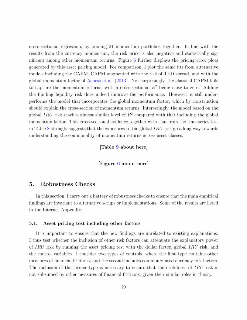
cross-sectional regression, by pooling 21 momentum portfolios together. In line with the

results from the currency momentum, the risk price is also negative and statistically sig-

nificant among other momentum returns. Figure 6 further displays the pricing error plots

generated by this asset pricing model. For comparison, I plot the same fits from alternative

models including the CAPM, CAPM augmented with the risk of TED spread, and with the

global momentum factor of Asness et al. (2013). Not surprisingly, the classical CAPM fails

to capture the momentum returns, with a cross-sectional R2 being close to zero. Adding

the funding liquidity risk does indeed improve the performance. However, it still under-

performs the model that incorporates the global momentum factor, which by construction

should explain the cross-section of momentum returns. Interestingly, the model based on the

global IRU risk reaches almost similar level of R2 compared with that including the global

momentum factor. This cross-sectional evidence together with that from the time-series test

in Table 8 strongly suggests that the exposures to the global IRU risk go a long way towards

understanding the commonality of momentum returns across asset classes.

[Table 9 about here]

[Figure 6 about here]

5. Robustness Checks

In this section, I carry out a battery of robustness checks to ensure that the main empirical

findings are invariant to alternative setups or implementations. Some of the results are listed

in the Internet Appendix.

5.1. Asset pricing test including other factors

It is important to ensure that the new findings are unrelated to existing explanations.

I thus test whether the inclusion of other risk factors can attenuate the explanatory power

of IRU risk by running the asset pricing test with the dollar factor, global IRU risk, and

the control variables. I consider two types of controls, where the first type contains other

measures of financial frictions, and the second includes commonly used currency risk factors.

The inclusion of the former type is necessary to ensure that the usefulness of IRU risk is

not subsumed by other measures of financial frictions, given their similar roles in theory.

20

To be more specific, I consider five measures of financial frictions: VIX and TED spread

of Brunnermeier et al. (2008), bond liquidity factor of Fontaine and Garcia (2011), betting

against beta factor of Frazzini and Pedersen (2014), and intermediary’s capital ratio of He

et al. (2017).16 For currency risk factors, I use the global FX volatility of Menkhoff et al.

(2012a), FX liquidity factor of Karnaukh et al. (2015), the recently proposed global equity

correlation of Bae and Elkamhi (2017),17 and the slope factors (high-minus-low returns) from

carry and momentum portfolios. Table 10 reports the results of asset pricing test of the

three-factor model via Fama-MacBeth regression, by using the joint cross-section of carry

and momentum portfolios as testing assets. For comparison, I also display the outcomes

from a model without using the IRU risk. While these competing risk factors fail to jointly

reconcile the carry and momentum returns, as manifested by the low R2, the explanatory

power of the global IRU risk is unaffected by adding in those controls. Moreover, despite

the significant risk prices for many control variables, partly due to the success of explaining

carry returns, their magnitudes of risk prices decrease substantially after adding in the global

IRU risk. Thus the evidence removes the concern that the information in the global IRU

risk is subsumed by other risk factors.

[Table 10 about here]

5.2. G10 carry and currency-level asset pricing

I evaluate whether the newly documented return-beta relation exists among some well-

known high or low interest rate currencies, such as the Australian Dollar (AUD) or Japanese

Yen (JPY). Panel A of Table 11 reports the excess returns and IRU betas after sorting

G10 currencies on their forward discounts. Interestingly, the return-beta relation found from

portfolio-level analysis also translates to G10 currencies. High interest rate currencies such

as AUD and NZD own the lowest negative IRU betas, whereas low interest rate currency

such as JPY and CHF possess the highest IRU betas.

On the other hand, as widely discussed in e.g., Ang et al. (2017), forming portfolios

for asset pricing test may destroy the information due to the shrinkage of cross-sectional

beta dispersions. I thus study the pricing power of IRU risk at the country-level carry and

16Since the leverage ratio of Adrian et al. (2014) is only available at the quarterly frequency, and He et al. (2017)show that their factor is the reciprocal of that of Adrian et al. (2014). I mainly focus on the monthly factor of Heet al. (2017). Quarterly results using the leverage ratio are similar and available upon request.

17The replicated series is plotted in Figure IA.2.

21

momentum trade. First, the conditional currency excess return for currency i is defined as

crxit+1 = citrxit+1, (16)

where I consider two ways of incorporating the conditional information:

ci1,t =

sign(f it − sit),

sign(rxit).ci2,t =

sign(f it − sit −med(ft − st)),

sign(rxit −med(rxt)).(17)

The first specification of sign functions follows Burnside et al. (2011) and Filippou et al.

(2018), and the second type is as in Della Corte and Krecetovs (2017), which represents the

sign of deviations from the cross-sectional median. These conditional returns are from the

managed long-short strategies on individual currencies based on their carry or momentum

signals. Since the panel of currency-level data is unbalanced, I follow Della Corte and

Krecetovs (2017) by using the Fama-MacBeth regression to estimate risk prices. Panel B of

Table 11 displays the results, where Newey-West standard errors are based on the estimated

series of risk prices, adjusted for the EIV problem of betas following Shanken (1992). The

outcomes point to the negative and almost significant pricing of the global IRU risk also at

the currency-level.

[Table 11 about here]

5.3. Subsample analysis

In this subsection, I assess the performance under a variety of subsamples over time and

countries, whose results are in Table 12. I first examine the performance of the global IRU

risk during the pre- and post-crisis sample, which are gapped by the period from July 2007 to

April 2010. The 2008 global financial crisis brings dramatic changes to the financial markets

and hence it is useful to evaluate the consistent pricing power of the global IRU risk before

and after the crisis. The carry and momentum trade implemented over the full universe of

currencies remain profitable in the pre-crisis (post-crisis) sample, with the monthly excess

returns of 0.50% and 0.46% (0.83% and 0.58%). Going through the asset pricing tests, I find

that the explanatory power of the global IRU risk is similar in both subsamples, with the

cross-sectional R2 reaching 81% and 85% respectively. The risk prices are also negative and

statistically significant.

22

Existing papers typically find that the momentum trade is not profitable among developed

countries (see, e.g., Karnaukh, 2016; Filippou et al., 2018). I thus study how the pricing

performance varies over carry and momentum returns by restricting the sample to include

only 21 developed economies.18 I find that although the carry trade is still profitable, the

profit from momentum strategy is indeed close to zero. Conforming to this fact, the pricing

power of the global IRU risk persists among carry portfolios, and the feeble momentum

returns is naturally accompanied with weak price of the global IRU risk.

As for other subsamples, I construct them by excluding the periods of extreme market

events that may be important to the FX market, such as the 1997 Asian financial crisis,

2008 global financial crisis, as well as the Euro-debt crisis.19 The pricing ability of the

global IRU risk remains hardly affected for these samples. Finally in Figure IA.3, I plot the

estimated IRU betas under all considered subsamples above for both carry and momentum

portfolios. It is clear that these betas still decline almost monotonically within the cross-

section of carry and momentum portfolios, justifying the robust role of the global IRU risk

as a unified explanation for these two currency strategies.

[Table 12 about here]

5.4. Additional robustness exercises

In the Internet Appendix, I report more results covering other aspects of robustness

concern. First, I evaluate the asset pricing performance on the momentum portfolios formed

over different window sizes, or formed by sorting on realized changes in log spot rates instead

of excess returns. The latter exercise is an important check since Menkhoff et al. (2012b)

show that there is a carry component within the momentum portfolios when sorting on

excess instead of simple returns. Table IA.1 and IA.2 show that although the performance

is slightly weaker for one-month momentum, with the joint cross-sectional R2 now reduces

to 86%, the main conclusions are largely unchanged: the high-minus-low beta spreads are

significant and the global IRU risk carries negative prices of risk.

Since the currency momentum may be tightly linked to the limits to arbitrage (e.g.

Menkhoff et al., 2012b), I test whether the role of IRU risk may be different for currencies

with different limits to arbitrage. Following Filippou et al. (2018), at each month and for each

18The detailed classification is in the Data Appendix.19To avoid specific dating of these crisis periods, I simply remove the data from Jan 1997 to Dec 1998, from July

2007 to April 2010, and from Jan 2011 to Dec 2012 respectively.

23

currency, I compute the idiosyncratic volatility (idvol) and skewness (idskew) that serve as

two measures for the limits to arbitrage.20 Then I run double sort by first forming two groups

of currencies based on their idiosyncratic volatility or skewness, and within each group, I form

three momentum portfolios. Table IA.3 and IA.4 report the IRU betas of these portfolios

and the results of asset pricing test. Whereas the profitability of FX momentum is generally

higher among the currencies with stronger limits to arbitrage, the high-minus-low spreads in

IRU betas are significant across these two groups of momentum portfolios. Also, compared

with the baseline asset pricing results, the magnitudes of most of the cross-sectional R2 are

still large. Therefore, the main empirical findings in this paper are unlikely driven by the

limits to arbitrage.

6. Conclusion

This paper documents the importance of the risk of global interest rate uncertainty on

accounting for the returns to FX carry and momentum trade. Empirically by using the

GDP-weighted average of G10 currencies’ interest rate realized variance as the measure for

the global interest rate uncertainty, I show that the return sensitivities of currency carry

and momentum portfolios to the global IRU shocks are almost monotonically decreasing

from the bottom to the top portfolios. The high-minus-low beta spreads are negative and

statistically significant. These risk exposures explain 89% and 97% of the cross-sectional

variations in mean returns of carry and momentum portfolios respectively. The negative and

significant correlations between the global IRU risk and returns to carry and momentum

trade are robust to other proxies for the global IRU , such as the realized volatility or the US

monetary policy uncertainty index of Baker et al. (2016). The explanatory power remains

significant under a variety of settings and robustness checks, and the global IRU risk is also

priced in momentum across other asset classes.

The economic reason behind the empirical success is the strong co-movements of the

global IRU risk with both strategy returns during their downturns. Existing studies find

that the crash behavior of carry and momentum differ substantially, which exacerbates the

difficulty of reconciling these returns in a unified way. I show that the global IRU risk

outperforms the commonly used risk factors such as the VIX or the global FX volatility on

achieving this task. It is significantly and negatively correlated with both strategy returns

under their respective crash periods. This channel is also consistent with an intermediary-

20The computation method follows Filippou et al. (2018) and is in the Internet Appendix.

24

based exchange rate model featuring the financial intermediary with limited risk-bearing

capacity, in the spirit of Gabaix and Maggiori (2015) and Mueller et al. (2017b). When

the intermediary’s constraint is close to bind, i.e., when either of the strategy is likely to

experience losses, rising global IRU will increase the shadow price of intermediary’s financial

constraint, leading to position unwinding by the intermediary. Such unwinding over long

positions (high carry/momentum currencies) and short positions (low carry/momentum cur-

rencies) generate opposite responses and hence the negative correlations between the global

IRU risk and returns to carry and momentum.

Appendix A. Data Appendix

The full dataset of currencies covers 48 countries from January 1985 to August 2017,

within which the classification of developed economies includes 21 countries: Australia,

Austria, Belgium, Canada, Denmark, Euro, Finland, France, Germany, Greece, Ireland,

Italy, Japan, Netherlands, New Zealand, Norway, Portugal, Spain, Sweden, Switzerland,

and the United Kingdom. The 27 developing economies cover Brazil, Bulgaria, Croatia,

Cyprus, Czech Republic, Egypt, Hong Kong, Hungary, Iceland, India, Indonesia, Israel,

Kuwait, Malaysia, Mexico, Philippines, Poland, Russia, Saudi Arabia, Singapore, Slovakia,

Slovenia, South Africa, South Korea, Taiwan, Thailand, and Ukraine. The series for the

euro start from January 1999 and I exclude the Eurozone currencies after that date. Due

to the large failures of covered interest rate parity, the following observations are removed

from the sample: South Africa from July 1985 to August 1985, Malaysia from August 1998

to June 2005, Indonesia from December 2000 to May 2007.

The final dates of all G10 daily interest rate data are as of August 2017, but the starting

months vary over countries and are listed in the following table.

25

Currency Starting month

AUD November 1999

CAD July 1989

CHF March 2007

DEM/EUR August 1990

GBP January 1992

JPY April 1989

NOK March 2007

NZD November 1999

SEK January 2007

USD January 1985

Other data include the daily FX returns, which are used to obtain global FX volatility

and correlation following Menkhoff et al. (2012a) and Mueller et al. (2017a). The daily bid-

ask spot and forward rates are used to construct the global FX liquidity measure following

Karnaukh et al. (2015). Finally, the TED spread and the VIX are downloaded from FRED,

whose samples start from January 1986 and January 1990 respectively.

Appendix B. Proof

Appendix B.1. Proof of Proposition

In equilibrium, the VaR constraint is binding due to the linear payoff function of the

financier. When Q is positive, we have:

P0(R∗e1 ≤ Re0) = α. (B.1)

If f1 is with the distribution function of F (·) and is independent of R and R∗, then (B.1)

can be expressed as ∫ f

f

P0(RQ+(f0 +Q)d1R

R∗d0

≥ z)dF (z) = α. (B.2)

Suppose that after the uncertainty shock to R and R∗, the distribution function P0(·)changes to P0(·). Due to the optimal behavior of the intermediary, Q will adjust to Q so

26

that the following equation holds∫ f

f

P0(RQ+(f0 + Q)d1R

R∗d0

≥ z)dF (z) = α. (B.3)

Then I rely on the property of uncertainty shock as derived by e.g. Diamond and Stiglitz

(1974) for the proof. The idea is that the uncertainty shock moves the probability mass

towards the tails of the distribution, without the change in the mean. Hence given z and Q,

denote the joint c.d.f of R∗ and R before and after positive uncertainty shock as G(·|z;Q)

and G(·|z;Q), then there exist two threshold values r∗ and r such that

1− G(R∗, R|z;Q) > 1−G(R∗, R|z;Q), if R∗ < r∗ and R > r. (B.4)

(B.4) in fact amounts to the following inequality when RQ+ (f0+Q)gRR∗ > rQ+ r

r∗g(f0 +Q)∫ f

f

P0(RQ+(f0 +Q)gR

R∗≥ z)dF (z) >

∫ f

f

P0(RQ+(f0 +Q)gR

R∗≥ z)dF (z), (B.5)

as long as the VaR limit α is small enough such that21

rQ+r

r∗g(f0 +Q) ≤ f. (B.6)

Now suppose that higher uncertainty by contradiction does not dampen the intermediary’s

risk-taking, that is, Q ≥ Q, then we have

α =

∫ f

f

P0(RQ+(f0 + Q)gR

R∗≥ z)dF (z) ≥

∫ f

f

P0(RQ+(f0 +Q)gR

R∗≥ z)dF (z). (B.7)

Due to (B.5), the last term of (B.7) satisfies∫ f

f

P0(RQ+(f0 +Q)gR

R∗≥ z)dF (z) >

∫ f

f

P0(RQ+(f0 +Q)gR

R∗≥ z)dF (z) = α, (B.8)

where the equality at the right-hand side reflects the optimality condition before the uncer-

tainty shock. Hence we obtain the contradiction.

Similar proof can be derived for the equilibrium Q < 0, where two threshold values are

21The inequality arises from the obvious fact that Q becomes lower when α decreases.

27

obtained such that R > r and R∗ > Rrr∗, and when α is small enough such that

rQ+r

r∗g(f0 +Q) ≥ f . (B.9)

Then to prove for the cross-sectional properties, note that Equation (B.2) can be further

expressed as ∫ f

f

∫ R

R

P0(R∗ ≤ (f0 +Q)d1r

(z − rQ)d0

)dG(r)dF (z) = α. (B.10)

Hence Q increases with E0(R∗) when Q > 0, since the threshold value in the parenthesis

has to increase so as the maintain the equality. Similarly, one can find that Q increases with

E0(R∗) also when Q < 0.

Meanwhile, one can also rewrite the Equation (B.2) as∫ f

f

∫ R

R

P0(d1

d0

≥ R∗(z − rQ)

(f0 +Q)r)dG(r)dF (z) = α. (B.11)

Hence Q decreases with E0(d1/d0) when Q > 0, since the threshold value in the parenthesis

has to increase so as the maintain the equality. Similarly, one can find that Q decreases with

E0(d1/d0) also when Q < 0.

References

Adrian, T., Etula, E., and Muir, T. (2014). Financial intermediaries and the cross-section

of asset returns. The Journal of Finance, 69(6):2557–2596.

Andrews, D. W. (1991). Heteroskedasticity and autocorrelation consistent covariance matrix

estimation. Econometrica, pages 817–858.

Ang, A., Liu, J., and Schwarz, K. (2017). Using individual stocks or portfolios in tests of

factor models.

Asness, C. S., Moskowitz, T. J., and Pedersen, L. H. (2013). Value and momentum every-

where. The Journal of Finance, 68(3):929–985.

Bae, J. W. and Elkamhi, R. (2017). Global equity correlation in fx carry and momentum

trades.

28

Baker, S. R., Bloom, N., and Davis, S. J. (2016). Measuring economic policy uncertainty.

The Quarterly Journal of Economics, 131(4):1593–1636.

Berg, K. A. and Mark, N. C. (2017). Measures of global uncertainty and carry-trade excess

returns. Journal of International Money and Finance.

Bloom, N. (2009). The impact of uncertainty shocks. Econometrica, 77(3):623–685.

Brogaard, J. and Detzel, A. (2015). The asset-pricing implications of government economic

policy uncertainty. Management Science, 61(1):3–18.

Brunnermeier, M. K., Nagel, S., and Pedersen, L. H. (2008). Carry trades and currency

crashes. NBER macroeconomics annual, 23(1):313–348.

Burnside, C. (2011). The cross section of foreign currency risk premia and consumption

growth risk: Comment. American Economic Review, 101(7):3456–76.

Burnside, C., Eichenbaum, M., Kleshchelski, I., and Rebelo, S. (2010). Do peso problems

explain the returns to the carry trade? The Review of Financial Studies, 24(3):853–891.

Burnside, C., Eichenbaum, M., and Rebelo, S. (2011). Carry trade and momentum in

currency markets. Annu. Rev. Financ. Econ., 3(1):511–535.

Cieslak, A. and Povala, P. (2016). Information in the term structure of yield curve volatility.

The Journal of Finance, 71(3):1393–1436.

Cochrane, J. H. (2005). Asset Pricing:(Revised Edition). Princeton University Press.

Corte, P. D., Riddiough, S. J., and Sarno, L. (2016). Currency premia and global imbalances.

The Review of Financial Studies, 29(8):2161–2193.

Daniel, K. and Moskowitz, T. J. (2016). Momentum crashes. Journal of Financial Eco-

nomics, 122(2):221–247.

Della Corte, P. and Krecetovs, A. (2017). Macro uncertainty and currency premia.

Della Corte, P., Sarno, L., Schmeling, M., and Wagner, C. (2016). Exchange rates and

sovereign risk.

Diamond, P. A. and Stiglitz, J. E. (1974). Increases in risk and in risk aversion. Journal of

Economic Theory, 8(3):337–360.

29

Dobrynskaya, V. (2014). Downside market risk of carry trades. Review of Finance,

18(5):1885–1913.

Dumas, B., Lewis, K. K., and Osambela, E. (2016). Differences of opinion and international

equity markets. The Review of Financial Studies, 30(3):750–800.

Filippou, I., Gozluklu, A., and Taylor, M. (2018). Global political risk and currency mo-

mentum. Journal of Financial and Quantitative Analysis.

Fontaine, J.-S. and Garcia, R. (2011). Bond liquidity premia. The Review of Financial

Studies, 25(4):1207–1254.

Frazzini, A. and Pedersen, L. H. (2014). Betting against beta. Journal of Financial Eco-

nomics, 111(1):1–25.

Gabaix, X. and Maggiori, M. (2015). International liquidity and exchange rate dynamics.

The Quarterly Journal of Economics, 130(3):1369–1420.

Hansen, L. P. and Jagannathan, R. (1997). Assessing specification errors in stochastic dis-

count factor models. The Journal of Finance, 52(2):557–590.

Hau, H. and Rey, H. (2005). Exchange rates, equity prices, and capital flows. The Review

of Financial Studies, 19(1):273–317.

He, Z., Kelly, B., and Manela, A. (2017). Intermediary asset pricing: New evidence from

many asset classes. Journal of Financial Economics, 126(1):1–35.

Jagannathan, R. and Wang, Z. (1996). The conditional capm and the cross-section of ex-

pected returns. The Journal of Finance, 51(1):3–53.

Kan, R. and Zhang, C. (1999). Two-pass tests of asset pricing models with useless factors.

the Journal of Finance, 54(1):203–235.

Karnaukh, N. (2016). Currency strategies and sovereign ratings.

Karnaukh, N., Ranaldo, A., and Soderlind, P. (2015). Understanding fx liquidity. The

Review of Financial Studies, 28(11):3073–3108.

Kozeniauskas, N., Orlik, A., and Veldkamp, L. (2018). What are uncertainty shocks? Journal

of Monetary Economics.

30

Kumhof, M. and Van Nieuwerburgh, S. (2007). Monetary policy in an equilibrium portfolio

balance model.

Lettau, M., Maggiori, M., and Weber, M. (2014). Conditional risk premia in currency

markets and other asset classes. Journal of Financial Economics, 114(2):197–225.

Lewellen, J., Nagel, S., and Shanken, J. (2010). A skeptical appraisal of asset pricing tests.

Journal of Financial Economics, 96(2):175–194.

Lustig, H., Roussanov, N., and Verdelhan, A. (2011). Common risk factors in currency

markets. Review of Financial Studies, page 37313777.

Lustig, H. and Verdelhan, A. (2007). The cross section of foreign currency risk premia and

consumption growth risk. American Economic Review, 97(1):89–117.

Lyons, R. K. (2001). The microstructure approach to exchange rates, volume 12. Citeseer.

Maio, P. and Santa-Clara, P. (2017). Short-term interest rates and stock market anomalies.

Journal of Financial and Quantitative Analysis, 52(3):927–961.

Menkhoff, L., Sarno, L., Schmeling, M., and Schrimpf, A. (2012a). Carry trades and global

foreign exchange volatility. The Journal of Finance, 67(2):681–718.

Menkhoff, L., Sarno, L., Schmeling, M., and Schrimpf, A. (2012b). Currency momentum

strategies. Journal of Financial Economics, 106(3):660–684.

Mueller, P., Stathopoulos, A., and Vedolin, A. (2017a). International correlation risk. Journal

of Financial Economics, 126(2):270–299.

Mueller, P., Tahbaz-Salehi, A., and Vedolin, A. (2017b). Exchange rates and monetary policy

uncertainty. The Journal of Finance, 72(3):1213–1252.

Newey, W. K. and West, K. (1987). A simple, positive semi-definite, heteroskedasticity and

autocorrelation consistent covariance matrix. Econometrica, 55(3):703–708.

Pastor, L. and Veronesi, P. (2012). Uncertainty about government policy and stock prices.

The Journal of Finance, 67(4):1219–1264.

Pastor, L. and Veronesi, P. (2013). Political uncertainty and risk premia. Journal of Financial

Economics, 110(3):520–545.

31

Patton, A. J. and Timmermann, A. (2010). Monotonicity in asset returns: New tests with

applications to the term structure, the capm, and portfolio sorts. Journal of Financial

Economics, 98(3):605–625.

Segal, G., Shaliastovich, I., and Yaron, A. (2015). Good and bad uncertainty: Macroeco-

nomic and financial market implications. Journal of Financial Economics, 117(2):369–397.

Shanken, J. (1992). On the estimation of beta-pricing models. The Review of Financial

Studies, 5(1):1–33.

Vayanos, D. and Woolley, P. (2013). An institutional theory of momentum and reversal. The

Review of Financial Studies, 26(5):1087–1145.

32

Table 1. Statistics of currency carry and momentum portfoliosThe table reports the statistics for the currency carry and momentum portfolios. Carry portfolios areobtained by sorting on the forward discounts, and momentum portfolios are obtained by sorting on therealized excess returns over the previous 3-month period. All portfolios are rebalanced monthly, and thereported average monthly excess returns (in percentage) are net of transaction costs. Exposures to the riskof global IRU are computed from Equation (4). The R2 of these regressions are listed in the last columnof each panel. Standard errors are in parentheses and based on Newey and West (1987) with optimal lagselection following Andrews (1991). The excess returns, IRU betas and monthly Sharpe ratios (SR) ofhigh-minus-low portfolios are also reported. The monotonicity of portfolio excess returns and IRU betasare tested via the monotonic relation (MR) test of Patton and Timmermann (2010), where the p-valuesare reported in parentheses based on all pair-wise comparisons. The null hypotheses for the tests are themonotonically increasing returns and decreasing betas respectively. The sample period is from January 1985to August 2017.

Panel A: Carry Panel B: Momentumre(%) βDOL βIRU re(%) βDOL βIRU

L -0.22 0.87 0.22 -0.10 1.02 0.22(0.12) (0.04) (0.07) (0.15) (0.08) (0.08)

2 0.05 0.91 0.06 -0.02 0.99 0.10(0.11) (0.03) (0.05) (0.12) (0.05) (0.05)

3 0.22 1.01 -0.09 0.17 1.02 -0.07(0.12) (0.03) (0.07) (0.12) (0.04) (0.10)

4 0.21 1.06 0.04 0.23 0.98 -0.05(0.13) (0.03) (0.06) (0.12) (0.04) (0.05)

H 0.36 1.16 -0.23 0.41 1.00 -0.22(0.17) (0.06) (0.13) (0.14) (0.07) (0.10)

HML 0.58 -0.44 0.51 -0.44(0.16) (0.18) (0.15) (0.16)

SR 0.21 0.17

MR (0.93) (0.97) (1.00) (0.92)

33

Table 2. Interest rate uncertainty of G10 currenciesPanel A reports the correlation coefficients of interest rate uncertainty for G10 currencies. For each economy,the interest rate uncertainty is estimated as the monthly realized variance of 10-year government bonds,computed from daily bond yields. Panel B reports the output from the principal component analysis onthe correlation matrix of G10 interest rate uncertainty. The pre-crisis sample is from January 1985 to June2007, and the post-crisis sample ranges from May 2010 to August 2017. Reported are the percentage of thetotal variance explained by each of the first three principal components.

Panel A: CorrelationAUD CAD CHF EUR GBP JPY NOK NZD SEK USD

AUD 1.00CAD 0.71 1.00CHF 0.78 0.75 1.00EUR 0.57 0.43 0.54 1.00GBP 0.56 0.53 0.59 0.57 1.00JPY 0.11 0.35 0.35 0.13 0.33 1.00NOK 0.67 0.64 0.61 0.70 0.55 0.18 1.00NZD 0.72 0.61 0.64 0.46 0.45 0.18 0.48 1.00SEK 0.73 0.72 0.69 0.76 0.71 0.16 0.75 0.61 1.00USD 0.71 0.39 0.69 0.54 0.38 0.10 0.50 0.59 0.60 1.00

Panel B: Principal component analysisFull sample Pre-crisis Post-crisis

First 59.9 54.1 59.9Second 10.9 11.7 11.8Third 8.3 8.7 7.8Total 79.1 74.5 79.5

34

Table 3. Correlation analysisThe table reports the correlation coefficients of returns to currency carry, momentum, global IRU risk, andother risk factors. These risk factors include the innovations to VIX, TED spread and global FX volatility;US consumption growth; NBER recession dummy, Fama-French small-minus-big (SMB) and high-minus-low(HML) factors. Significance of correlations is only displayed for quantities related to carry and momentumreturns, where *, **, and *** indicate statistical significance at 10%, 5%, and 1% levels. The sample periodis from January 1985 to August 2017.

VIX TED spread Global FX vol US growth NBER recession SMB HML Global IRU Carry Momentum

VIX 1.00

TED spread 0.22 1.00

Global FX vol 0.35 0.11 1.00

US growth -0.02 -0.01 0.06 1.00

NBER recession 0.12 0.03 0.14 -0.29 1.00

SMB -0.21 -0.06 0.01 0.09 0.05 1.00

HML 0.09 0.08 0.01 -0.08 -0.07 -0.27 1.00

Global IRU 0.47 0.20 0.20 0.04 0.10 -0.10 0.01 1.00

Carry -0.26*** -0.05 -0.35*** -0.09* -0.01 0.06 -0.07 -0.16*** 1.00

Momentum 0.01 -0.07 0.04 0.02 0.01 0.02 -0.05 -0.15*** 0.03 1.00

35

Table 4. Cross-sectional asset pricing testThe table reports the results of asset pricing test for the two-factor model containing the dollar factor and theglobal IRU risk (uIRU

t ), or its factor-mimicking portfolio returns (uIRUFMM,t). The factor-mimicking portfolio

is constructed by projecting uIRUt on the return space of five carry and five momentum portfolios. Panel

A and B display the test results via Fama-MacBeth regression, where I report the estimated risk prices,cross-sectional OLS R2, the heteroskedastic and autocorrelation consistent (HAC) standard errors basedon Newey and West (1987) with optimal lag selection following Andrews (1991) (NW), and the Shanken-adjusted standard errors of Shanken (1992) (Sh). The p-values of χ2-test on the null hypothesis that thepricing errors are jointly zero are also reported. Panel C and D display the test results via the GMMestimation, where I report the estimated factor loadings in the SDF model (7) by using the optimal weightmatrix in the estimation. The Newey-West standard errors are in parentheses. I also report the p-valuesfrom the χ2-test, and the estimated Hansen-Jagannathan distances and their p-values, which are obtainedvia simulation following Jagannathan and Wang (1996). The testing assets are the carry, momentum ortheir joint cross-sectional portfolios. The sample period is from January 1985 to August 2017.

Carry Momentum Carry+MomentumPanel A: Fama-MacBeth

λDOL λIRU R2 λDOL λIRU R2 λDOL λIRU R2

0.13 -1.16 0.89 0.13 -1.19 0.97 0.13 -1.18 0.92(NW) (0.11) (0.34) (0.11) (0.33) (0.11) (0.28)(Sh) (0.11) (0.53) (0.11) (0.52) (0.11) (0.42)χ2NW [0.14] [0.66] [0.05]χ2Sh [0.51] [0.88] [0.60]

Panel B: Fama-MacBeth using factor-mimicking portfolioλDOL λIRU R2 λDOL λIRU R2 λDOL λIRU R2

0.13 -0.30 0.89 0.13 -0.31 0.97 0.13 -0.30 0.92(NW) (0.11) (0.08) (0.11) (0.08) (0.11) (0.06)(Sh) (0.11) (0.08) (0.11) (0.08) (0.11) (0.06)χ2NW [0.14] [0.66] [0.05]χ2Sh [0.17] [0.69] [0.08]

Panel C: GMMbDOL bIRU R2 bDOL bIRU R2 bDOL bIRU R2

coef 0.05 -1.24 0.87 0.05 -1.57 0.87 0.04 -1.52 0.76s.e. (0.04) (0.58) (0.04) (0.62) (0.03) (0.49)

χ2-test [0.36] [0.89] [0.49]HJ-dist 0.13 0.07 0.19

[0.28] [0.80] [0.34]Panel D: GMM using factor-mimicking portfolio

bDOL bIRU R2 bDOL bIRU R2 bDOL bIRU R2

coef 0.04 -0.30 0.87 0.04 -0.31 0.96 0.04 -0.33 0.91s.e. (0.03) (0.07) (0.03) (0.09) (0.03) (0.06)

χ2-test [0.20] [0.73] [0.19]HJ-dist 0.13 0.07 0.19

[0.00] [0.04] [0.00]

36

Table 5. Asset pricing tests with alternative measures for global IRU riskThe table reports the results of asset pricing test by using three alternative measures for the global IRUrisk based on: equal-weighted average of realized variance; GDP-weighted average of realized volatility;and the US Monetary Policy Uncertainty index of Baker et al. (2016). In each panel, I first report theestimated IRU betas of carry and momentum portfolios together with their Newey-West standard errors.Then I display the results of asset pricing test via the Fama-MacBeth cross-sectional regression, where Ireport the estimated risk prices, cross-sectional OLS R2, the heteroskedastic and autocorrelation consistent(HAC) standard errors based on Newey and West (1987) with optimal lag selection following Andrews (1991)(NW), and the Shanken-adjusted standard errors of Shanken (1992) (Sh). The p-values of χ2-test on thenull hypothesis that the pricing errors are jointly zero are also reported. The testing assets are the carry,momentum or their joint cross-sectional portfolios. The sample period is from January 1985 to August 2017.

Panel A: Equal-weighted average of realized varianceL 2 3 4 H HML

βCIRU 0.24 0.05 -0.10 0.04 -0.24 -0.48

(0.06) (0.05) (0.07) (0.06) (0.12) (0.16)βMIRU 0.24 0.13 -0.08 -0.07 -0.24 -0.48

(0.07) (0.04) (0.09) (0.06) (0.09) (0.14)

λCIRU -1.08 R2 0.90 χ2Sh [0.48]

(Sh) (0.46)λMIRU -1.05 R2 0.97 χ2

Sh [0.91](Sh) (0.42)

λC+MIRU -1.06 R2 0.93 χ2

Sh [0.59](Sh) (0.36)

Panel B: GDP-weighted average of realized volatilityL 2 3 4 H HML

βCIRU 0.19 0.10 -0.11 0.01 -0.19 -0.38

(0.08) (0.05) (0.06) (0.06) (0.13) (0.18)βMIRU 0.15 0.09 -0.02 -0.06 -0.17 -0.32

(0.11) (0.06) (0.09) (0.05) (0.11) (0.20)

λCIRU -1.27 R2 0.90 χ2Sh [0.52]

(Sh) (0.57)λMIRU -1.61 R2 0.99 χ2

Sh [0.99](Sh) (0.83)

λC+MIRU -1.41 R2 0.93 χ2

Sh [0.78](Sh) (0.56)

Panel C: BBD MPU indexL 2 3 4 H HML

βCIRU 0.18 0.05 -0.04 -0.04 -0.16 -0.34

(0.07) (0.05) (0.04) (0.06) (0.09) (0.15)βMIRU 0.21 0.10 -0.04 -0.07 -0.19 -0.40

(0.10) (0.06) (0.06) (0.05) (0.10) (0.17)

λCIRU -1.64 R2 0.98 χ2Sh [0.97]

(Sh) (0.90)λMIRU -1.29 R2 0.98 χ2

Sh [0.99](Sh) (0.57)

λC+MIRU -1.42 R2 0.96 χ2

Sh [0.63](Sh) (0.56)

37

Table 6. Comovements with risk factors when carry or momentum failsThe table reports the correlation coefficients of the risk of global IRU , VIX, global FX volatility and returnsto carry (rCt ) and momentum (rMt ) trade, computed over different crashing periods for two strategies. Thecrash periods are identified as the months when current strategy returns are below the k-th percentile of theempirical distribution of strategy returns. The average monthly strategy returns during the crash periodsand the significance of correlations are also reported, where *, **, and *** indicate statistical significance at10%, 5%, and 1% levels. The sample period is from January 1985 to August 2017.

Percentile (k) < 10 < 20 < 30 < 40 < 50Panel A: When carry fails

Corr(uIRUt , rCt ) −0.29* −0.26** −0.27*** −0.28*** −0.24***

Corr(uIRUt , rMt ) −0.38** −0.31*** −0.24*** −0.20** −0.18**

Corr(uV IXt , rCt ) −0.09 −0.13 −0.18* −0.22*** −0.22***

Corr(uV IXt , rMt ) −0.03 0.01 −0.02 0.01 −0.01

Corr(uFXV OLt , rCt ) −0.17 −0.31*** −0.37*** −0.41*** −0.42***

Corr(uFXV OLt , rMt ) 0.24 0.25** 0.23** 0.24*** 0.21***

E(rCt )(%) −5.10 −3.38 −2.49 −1.86 −1.38Panel B: When momentum fails

Corr(uIRUt , rCt ) −0.39** −0.36*** −0.33*** −0.30*** −0.29***

Corr(uIRUt , rMt ) −0.38*** −0.38*** −0.37*** −0.33*** −0.30***

Corr(uV IXt , rCt ) −0.37** −0.30*** −0.30*** −0.31*** −0.28***

Corr(uV IXt , rMt ) −0.31* −0.17 −0.09 −0.06 −0.06

Corr(uFXV OLt , rCt ) −0.33** −0.25** −0.29*** −0.27*** −0.29***

Corr(uFXV OLt , rMt ) −0.23 −0.23** −0.27*** −0.30*** −0.28***

E(rMt )(%) −4.84 −3.44 −2.67 −2.13 −1.67

38

Table 7. Cross-sectional predictability of foreign currency supply by currency returnsThe table reports the results of using currency returns to predict future supply of foreign currency inexchange for USD. For each country, −∆st−j:t is the currency return (vis-a-vis USD) between month t− j tot, log dt+h − log dt is the log change of country’s equity purchases from US between month t to t+ h, whichserved as the proxy for the growth of foreign currency supply. The forecasting horizon h ranges from one- tothree-month. Panel A to C correspond to the results for j = 1, 3 and 6. The left part of each panel reportsthe time series average of log dt+h − log dt for portfolios formed by sorting on currency return −∆st−j:t atthe end of month-t, and the right part displays the average slope coefficients from the currency-level Fama-MacBeth cross-sectional regression (15). Reported R2 is the time-series average of cross-sectional R2 fromthe regressions. All t-statistics are reported in the parentheses and based on the standard errors of Neweyand West (1987) with the optimal lag selection of Andrews (1991). The sample period is from January 1985to August 2017.

Portfolio approach Fama-MacBethL 2 3 4 H HML b R2(%)

Panel A: MOM11 (−∆st−1:t on log dt+h − log dt)

h = 1 1.84 2.35 1.41 1.20 0.80 -1.53 -0.27 3.57(t) (1.99) (2.40) (1.69) (1.53) (1.04) (-1.46) (-1.61)

h = 2 3.84 3.49 2.60 2.04 2.84 -1.65 -0.11 3.71(t) (3.51) (2.98) (2.43) (1.85) (2.80) (-1.52) (-0.59)

h = 3 6.05 5.00 4.51 4.48 3.51 -2.87 -0.33 4.21(t) (4.77) (3.65) (3.56) (3.39) (3.00) (-2.58) (-1.63)

Panel B: MOM31 (−∆st−3:t on log dt+h − log dt)

h = 1 0.79 3.81 2.31 0.88 0.52 -0.09 -3.75 3.89(t) (0.91) (4.29) (2.66) (0.99) (0.66) (-0.65) (-1.17)

h = 2 2.34 5.25 4.30 1.20 1.51 -1.16 -0.23 4.19(t) (2.15) (4.44) (3.99) (1.00) (1.48) (-0.99) (-2.18)

h = 3 4.77 6.98 5.68 3.44 2.82 -2.33 -0.29 4.58(t) (3.50) (5.54) (4.51) (2.62) (2.33) (-1.74) (-2.25)

Panel C: MOM61 (−∆st−6:t on log dt+h − log dt)

h = 1 2.35 1.12 2.65 1.65 0.31 -2.49 -0.09 4.70(t) (2.75) (1.42) (3.32) (2.04) (0.38) (-2.50) (-1.61)

h = 2 4.07 3.80 3.78 2.88 1.31 -2.92 -0.15 4.37(t) (3.40) (3.53) (3.43) (2.48) (1.25) (-2.39) (-2.11)

h = 3 6.00 5.22 4.16 4.76 3.11 -3.43 -0.24 4.92(t) (4.30) (4.36) (3.37) (3.48) (2.43) (-2.54) (-2.82)

39

Table 8. Momentum everywhere and global IRU riskThe table reports the results of time-series regression (3) by projecting momentum returns in different assetclasses on the global IRU risk or the funding liquidity risk, proxied by the innovations to the TED spread.All t-statistics are reported in the parentheses and based on the standard errors of Newey and West (1987)with the optimal lag selection of Andrews (1991). The sample period is from January 1985 to August 2017.

E(rMOMt )(%) βIRU (%) βTED(%) βIRU (%)

US equities 0.31 -0.39 -0.23 -0.44(1.38) (-2.34) (-1.08) (-2.62)

UK equities 0.64 -0.48 -0.39 -0.41(2.59) (-3.19) (-1.68) (-2.28)

Europe equities 0.41 -0.20 -0.25 -0.18(1.84) (-1.44) (-1.40) (-1.22)

Japan equities 0.15 -0.39 0.16 -0.46(0.52) (-2.18) (0.65) (-2.01)

Equity indices 0.49 -0.45 -0.07 -0.54(3.11) (-1.54) (-0.41) (-2.01)

Fixed income -0.01 0.02 -0.04 -0.04(-0.02) (0.21) (-0.46) (-0.49)

Commodities 0.73 -0.64 0.10 -0.75(2.68) (-2.69) (0.33) (-2.57)

Global Mom 0.34 -0.30 -0.12 -0.33(3.01) (-3.52) (-1.43) (-4.12)

40

Table 9. Pricing momentum returns across asset classesThe table reports the results of cross-sectional asset pricing test using the asset pricing model with the marketfactor and the global IRU risk. The test is done via the Fama-MacBeth regression, where I report the first-stage estimated betas for each asset class, and the second-stage estimated risk price by pooling 21 momentumportfolios together. I also report the cross-sectional OLS R2, the t-statistics based on the heteroskedasticand autocorrelation consistent (HAC) standard errors pf Newey and West (1987) with optimal lag selectionfollowing Andrews (1991), or based on the Shanken-adjusted standard errors of Shanken (1992) (Sh). Iimpose zero intercept in the second-stage regression. The sample period is from January 1985 to August2017.

L M H HML L M H HMLUS equities UK equities

Return (%) 0.55 0.62 0.86 0.31 0.24 0.81 0.88 0.64(2.02) (2.99) (3.48) (1.38) (0.68) (3.23) (3.00) (2.59)

CAPM beta 0.94 0.75 0.83 -0.11 1.15 0.87 0.93 -0.23(14.50) (20.79) (15.91) (-1.29) (15.29) (20.21) (18.55) (-2.98)

IRU beta 0.15 -0.28 -0.33 -0.48 0.00 -0.34 -0.66 -0.66(1.07) (-1.84) (-2.03) (-2.32) (0.02) (-1.86) (-3.32) (-3.22)

Europe equities Japan equitiesReturn (%) 0.59 0.82 1.00 0.41 0.23 0.27 0.39 0.15

(1.77) (3.06) (3.50) (1.84) (0.63) (0.87) (1.14) (0.52)CAPM beta 1.13 0.93 0.92 -0.21 0.97 0.89 0.86 -0.11

(10.16) (12.97) (13.49) (-2.44) (10.72) (11.80) (9.31) (-1.42)IRU beta -0.05 -0.14 -0.41 -0.36 0.88 0.39 0.40 -0.48

(-0.26) (-0.79) (-2.12) (-2.22) (3.70) (1.65) (1.64) (-2.47)Equity indices Fixed-income

Return (%) 0.30 0.63 0.78 0.49 0.33 0.23 0.32 -0.01(1.10) (2.54) (2.99) (3.11) (3.79) (2.67) (3.62) (-0.02)

CAPM beta 0.86 0.80 0.81 -0.05 0.01 0.00 0.01 0.01(12.65) (20.67) (18.29) (-0.75) (0.23) (0.02) (0.56) (0.44)

IRU beta -0.34 -0.26 -0.83 -0.48 0.00 -0.04 0.03 0.02(-2.44) (-1.94) (-4.40) (-1.78) (0.04) (-0.46) (0.19) (0.29)

Commodities Pricing test with 21 portfoliosReturn (%) -0.04 0.09 0.69 0.73 Risk price -0.51

(-0.17) (0.40) (2.56) (2.68) NW (t) (-2.53)CAPM beta 0.33 0.30 0.27 -0.07 Sh (t) (-2.27)

(4.38) (3.78) (2.18) (-0.87)IRU beta 0.44 0.22 -0.25 -0.69 R2 0.44

(2.08) (1.38) (-1.09) (-2.97)

41

Table 10. Robustness: Pricing power of IRU risk under controlsThe table reports the results of asset pricing test on the joint cross-section of currency carry and momentumportfolios, by including other control variables in addition to the global IRU risk. Panel A contains thecontrols measuring the financial frictions: VIX and TED spread, the bond liquidity factor of Fontaine andGarcia (2011), betting against beta factor of Frazzini and Pedersen (2014), and intermediary’s capital ratioof He et al. (2017). Panel B contains the commonly used currency risk factors: the global FX volatility ofMenkhoff et al. (2012a), FX liquidity factor of Karnaukh et al. (2015), global equity correlation of Bae andElkamhi (2017), and the high-minus-low returns of carry and momentum portfolios respectively. The testis done via Fama-MacBeth regression, where I report the estimated risk prices, cross-sectional OLS R2, theheteroskedastic and autocorrelation consistent (HAC) standard errors based on Newey and West (1987) withoptimal lag selection following Andrews (1991) (NW), and the Shanken-adjusted standard errors of Shanken(1992) (Sh). The p-values of χ2-test on the null hypothesis that the pricing errors are jointly zero are alsoreported. The sample period is from January 1985 to August 2017.

Panel A: Other measures of financial frictionsX VIX TED Bond liquidity BAB Capital ratioλX -0.68 -0.49 -1.84 -0.35 -0.90 0.32 1.76 -0.29 0.49 0.24

(NW) (0.22) (0.21) (0.49) (0.51) (0.40) (0.37) (0.56) (0.45) (0.23) (0.23)(Sh) (0.27) (0.31) (1.01) (0.76) (0.53) (0.56) (1.13) (0.74) (0.25) (0.32)

λIRU -1.08 -1.06 -0.98 -1.19 -1.06(NW) (0.25) (0.26) (0.25) (0.28) (0.32)(Sh) (0.37) (0.38) (0.37) (0.45) (0.45)

R2 0.33 0.87 0.53 0.87 0.09 0.87 0.32 0.94 0.37 0.91

χ2NW [0.00] [0.03] [0.00] [0.04] [0.00] [0.05] [0.00] [0.06] [0.01] [0.11]χ2Sh [0.02] [0.44] [0.73] [0.45] [0.02] [0.52] [0.37] [0.66] [0.05] [0.56]

Panel B: Other currency risk factorsX FX Vol FX liquidity GEC HMLcarry HMLmom

λX -0.46 -0.30 -0.74 -0.02 -0.81 -0.14 0.19 0.21 0.19 0.18(NW) (0.17) (0.17) (0.35) (0.34) (0.37) (0.38) (0.05) (0.05) (0.05) (0.05)(Sh) (0.19) (0.25) (0.44) (0.53) (0.47) (0.59) (0.05) (0.06) (0.05) (0.05)

λIRU -1.15 -1.18 -1.20 -1.15 -1.13(NW) (0.28) (0.28) (0.28) (0.32) (0.36)(Sh) (0.42) (0.43) (0.44) (0.48) (0.53)

R2 0.32 0.93 0.20 0.92 0.26 0.93 0.45 0.92 0.55 0.92

χ2NW [0.00] [0.04] [0.00] [0.04] [0.00] [0.04] [0.00] [0.05] [0.00] [0.03]χ2Sh [0.00] [0.52] [0.00] [0.53] [0.01] [0.55] [0.00] [0.53] [0.00] [0.43]

42

Table 11. Robustness: Currency-level asset pricingThe table reports the results of currency-level asset pricing. Panel A reports the forward discounts, excessreturns and IRU betas of G10 currencies (excl. USD). Panel B reports the estimated risk prices from theFama-MacBeth regression by using the conditional currency excess returns of individual currencies. C1 isbased on the conditional excess return that is defined as the raw excess return multiplied by the sign functionof lagged interest rate differential or realized excess return, and C2 uses the sign function of the deviationfrom the cross-sectional median of lagged interest rate differential or realized excess return (detailed inEquation (17)). The Newey-West HAC standard errors are in parentheses with the optimal lag selectionfollowing Andrews (1991), and adjusted for the EIV problem of betas following Shanken (1992). The sampleperiod is from January 1985 to August 2017.

Panel A: G10 currencyForward discount Excess return IRU beta

CHF -1.92 0.02 0.41JPY -1.25 0.14 0.23

DEM/EUR -0.35 0.14 0.10CAD 0.63 0.08 -0.15SEK 1.18 0.15 0.06GBP 1.45 0.18 0.04NOK 1.65 0.21 -0.02NZD 2.55 0.25 -0.34AUD 3.44 0.45 -0.25

Panel B: Conditional currency returnsC1 C2

λDOL λIRU λDOL λIRU

Carry 3.93 -0.18 2.37 -0.35(NW) (1.51) (0.21) (1.37) (0.18)

MOM -9.99 -0.58 -2.69 -0.22(NW) (5.93) (0.21) (3.97) (0.19)

Carry+MOM 3.18 -0.40 2.14 -0.26(NW) (1.56) (0.16) (1.39) (0.14)

43

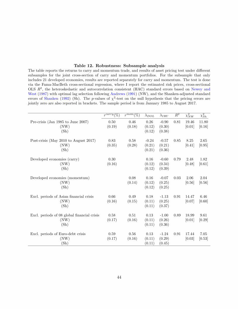
Table 12. Robustness: Subsample analysisThe table reports the returns to carry and momentum trade, and results of asset pricing test under differentsubsamples for the joint cross-section of carry and momentum portfolios. For the subsample that onlyincludes 21 developed economies, results are reported separately for carry and momentum. The test is donevia the Fama-MacBeth cross-sectional regression, where I report the estimated risk prices, cross-sectionalOLS R2, the heteroskedastic and autocorrelation consistent (HAC) standard errors based on Newey andWest (1987) with optimal lag selection following Andrews (1991) (NW), and the Shanken-adjusted standarderrors of Shanken (1992) (Sh). The p-values of χ2-test on the null hypothesis that the pricing errors arejointly zero are also reported in brackets. The sample period is from January 1985 to August 2017.

rcarry(%) rmom(%) λDOL λIRU R2 χ2NW χ2

Sh

Pre-crisis (Jan 1985 to June 2007) 0.50 0.46 0.26 -0.90 0.81 19.46 11.80(NW) (0.19) (0.18) (0.12) (0.30) [0.01] [0.16](Sh) (0.12) (0.38)

Post-crisis (May 2010 to August 2017) 0.83 0.58 -0.24 -0.57 0.85 8.25 2.65(NW) (0.35) (0.28) (0.21) (0.21) [0.41] [0.95](Sh) (0.21) (0.36)

Developed economies (carry) 0.30 0.16 -0.60 0.79 2.48 1.82(NW) (0.16) (0.12) (0.34) [0.48] [0.61](Sh) (0.12) (0.39)

Developed economies (momentum) 0.08 0.16 -0.07 0.03 2.06 2.04(NW) (0.14) (0.12) (0.25) [0.56] [0.56](Sh) (0.12) (0.25)

Excl. periods of Asian financial crisis 0.66 0.49 0.18 -1.13 0.91 14.47 6.46(NW) (0.16) (0.15) (0.11) (0.25) [0.07] [0.60](Sh) (0.11) (0.37)

Excl. periods of 08 global financial crisis 0.58 0.51 0.13 -1.00 0.89 18.99 9.61(NW) (0.17) (0.16) (0.11) (0.26) [0.01] [0.29](Sh) (0.11) (0.36)

Excl. periods of Euro-debt crisis 0.59 0.56 0.13 -1.24 0.91 17.44 7.05(NW) (0.17) (0.16) (0.11) (0.29) [0.03] [0.53](Sh) (0.11) (0.45)

44

Figure 1. Global interest rate uncertainty and its innovations

The upper panel plots the level of global interest rate uncertainty, computed as the GDP-weighted realizedvariance of 10-year government bond yields of G10 currencies. The lower panel plots the standardizedinnovations uIRU

t , obtained from fitting an AR(1) model to the level series. The sample period is fromJanuary 1985 to August 2017.

1985 1990 1995 2000 2005 2010 20150

0.1

0.2

0.3

0.4

0.5

0.6

0.7

0.8

0.9Global IRU

1985 1990 1995 2000 2005 2010 2015-6

-4

-2

0

2

4

6

8

10

12

14Standardized Innovations to Global IRU

45

Figure 2. Carry and momentum returns conditional on global IRU risk

The figure plots the performance of carry (left panel) and momentum (right two panels) strategy conditionalon four quartiles of the empirical distribution of innovations to the global IRU . The momentum tradeare based on either one-month (middle panel) or three-month (right panel) formation window. The sampleperiod is from January 1985 to August 2017.

Low 2 3 HighDistribution of innovations to Global IRU

0

2

4

6

8

10

12

14

Ann

ualiz

ed a

vera

ge r

etur

ns (

%)

Returns to carry trade

Low 2 3 HighDistribution of innovations to Global IRU

0

1

2

3

4

5

6

7

8

9

Ann

ualiz

ed a

vera

ge r

etur

ns (

%)

Returns to momentum trade (1M)

Low 2 3 HighDistribution of innovations to Global IRU

0

1

2

3

4

5

6

7

8

Ann

ualiz

ed a

vera

ge r

etur

ns (

%)

Returns to momentum trade (3M)

46

Figure 3. Global IRU betas and pricing error plots

The upper panel plots the sensitivities of carry and momentum portfolio returns to the risk of global un-certainty (IRU betas), which are estimated from Equation (4). The lower panel plots the portfolio meanreturns and fitted returns from the asset pricing model containing the dollar factor and the global IRUrisk, estimated over carry and momentum portfolio separately. The sample period is from January 1985 toAugust 2017.

Low 2 3 4 High-0.2

-0.15

-0.1

-0.05

0

0.05

0.1

0.15

0.2

0.25

0.3Carry

Low 2 3 4 High-0.2

-0.15

-0.1

-0.05

0

0.05

0.1

0.15

0.2

0.25

0.3Momentum

1 2 3 4 5-0.3

-0.2

-0.1

0

0.1

0.2

0.3

0.4

0.5

Ret

urns

(%)

DataFitted

1 2 3 4 5-0.3

-0.2

-0.1

0

0.1

0.2

0.3

0.4

0.5

Ret

urns

(%)

DataFitted

47

Figure 4. Market states and global IRU risk when carry or momentum fails

The upper (lower) panel plots the average of US aggregate stock returns (innovations to the global interestrate uncertainty) when currency carry or momentum strategy experiences sizable losses as defined in Equation(10). The sample period is from January 1985 to August 2017.

<10 <20 <30 <40 <500

0.2

0.4

0.6

Inn

ova

tion

s t

o g

lob

al IR

U CarryMomentum

<10 <20 <30 <40 <50-20

-10

0

10

20

An

nu

alize

d m

ark

et re

turn

(%

)

CarryMomentum

48

Figure 5. Global IRU risk during bad and good states

The figure plots the average of innovations to the global interest rate uncertainty when the economy is inbad or good states contemporaneously. The measure of the economic activity is the US industrial productiongrowth, the Chicago Fed National Activity Index (CFNAI), and the aggregate market returns. The definitionof bad or good states follows similarly the Equation (10). The sample period is from January 1985 to August2017.

<10 <20 <30 >70 >80 >90-0.5

0

0.5Industrial production growth

<10 <20 <30 >70 >80 >90-0.5

0

0.5CFNAI

<10 <20 <30 >70 >80 >90-0.5

0

0.5Market return

49

Figure 6. Pricing error plots for momentum everywhere

The figure contains the scatter plots between average portfolio excess returns and the fitted excess returnsfrom the asset pricing model described in each panel. The model is estimated via the two-stage Fama-MacBeth regression. Zero intercept is imposed when running the second-stage cross-sectional regression.The sample period is from January 1985 to August 2017.

-0.5 0 0.5 1 1.5-0.5

0

0.5

1

1.5CAPM R2= 0.01

US.M1US.M2

US.M3

UK.M1

UK.M2UK.M3

EUR.M1

EUR.M2 EUR.M3JP.M1JP.M2 JP.M3EI.M1 EI.M2 EI.M3

FI.M1FI.M2FI.M3

Cmdty.M1Cmdty.M2 Cmdty.M3

-0.5 0 0.5 1-0.5

0

0.5

1CAPM+TED R2= 0.35

US.M1US.M2

US.M3

UK.M1

UK.M2

UK.M3

EUR.M1EUR.M2

EUR.M3

JP.M1

JP.M2

JP.M3

EI.M1EI.M2

EI.M3

FI.M1FI.M2FI.M3

Cmdty.M1

Cmdty.M2

Cmdty.M3

-0.5 0 0.5 1 1.5-0.5

0

0.5

1

1.5CAPM+MOM R2= 0.46

US.M1

US.M2

US.M3

UK.M1

UK.M2

UK.M3

EUR.M1

EUR.M2

EUR.M3

JP.M1

JP.M2

JP.M3

EI.M1EI.M2

EI.M3

FI.M1FI.M2FI.M3

Cmdty.M1

Cmdty.M2

Cmdty.M3

-0.5 0 0.5 1 1.5-0.5

0

0.5

1

1.5CAPM+IRU R2= 0.44

US.M1US.M2

US.M3UK.M1 UK.M2

UK.M3

EUR.M1EUR.M2

EUR.M3

JP.M1

JP.M2 JP.M3

EI.M1EI.M2

EI.M3

FI.M1FI.M2FI.M3Cmdty.M1Cmdty.M2

Cmdty.M3

50

Internet Appendix to “Currency Carry, Momentum, and GlobalInterest Rate Uncertainty” (not for publication)

A. Adjustment for transaction costs, calculation of idiosyncratic

volatility and skewness

Following Menkhoff et al. (2012b) and many others, at the end of month t+ 1, and for

currency i, if it leaves the sorted portfolio that is formed at month t after t+ 1, then the

net excess return for the lowest portfolio (the portfolio being shorted) is computed as

rxst+1 = fat − sbt+1, (IA.1)

where the superscripts a and b represent the ask and bid prices. For the long portfolios

above the bottom one, the net excess returns are

rxlt+1 = f bt − sat+1. (IA.2)

On the other hand, if currency i does not leave the current portfolio, then the excess

returns are computed as

rxst+1 = fat − st+1, rxlt+1 = f b

t − st+1. (IA.3)

To compute two measures of the limits to arbitrage for each currency i, I follow Filippou

et al. (2018) by first extracting the residual series from the following asset pricing model

rxit = αi + βi1DOLt + β2HMLcarry,t + εi,t, (IA.4)

where DOLt and HMLcarry,t are the daily dollar factor and the slope factor from carry

trade portfolios. This asset pricing model is proposed by Lustig et al. (2011), and the

regression is estimated by using daily data within each month. Then the currency i’s

idiosyncratic volatility and skewness at month-T are computed as

IVi,T =

√∑NT

j=1 ε2i,d

NT

, ISi,T =

∑NT

j=1 ε3i,d

NT (IVi,T )3, (IA.5)

1

where NT denotes the number of daily returns available during month-T .

B. Extracting risk factor from the BBD MPU index

The US Monetary Policy Uncertainty (MPU) index built by Baker et al. (2016) is

constructed as the scaled frequency counts of articles that discuss US monetary policy

uncertainty, from hundreds of US daily newspapers covered by Access World News. To

obtain their shocks as the risk factor, I follow Della Corte and Krecetovs (2017) by first

computing the simple change in MPU level:

∆MPUt = MPUt −MPUt−1. (IA.6)

However, ∆MPUt is highly correlated with changes in other category-specific BBD policy

uncertainty indexes,22 which confound the identification of shocks. I thus run the following

orthogonalization:

∆MPUt = α +∑j

βj∆EPUj,t + uMPUt , (IA.7)

where EPUj,t denotes the BBD policy uncertainty index of category-j, and uMPUt denotes

the orthogonal MPU shocks used in the paper. For variables on the right-hand side of

Equation (IA.7), I consider four categories that cover Taxes; Fiscal and government

spending; Sovereign debt; and National security. The selection follows their relevance for

FX markets (see, e.g., Kumhof and Van Nieuwerburgh, 2007; Della Corte et al., 2016) and

results are not sensitive to other choices.

C. Supplementary results

22In addition to the uncertainty over monetary policy, Baker et al. (2016) also builds the policy uncertainty indexesfor the categories such as the fiscal policy, sovereign debt, etc.

2

Table IA.1. Statistics of alternative momentum portfoliosThe table reports the statistics for the currency momentum portfolios, which are obtained by sorting onthe realized excess returns over the previous 1- and 6-month periods. Alternatively, I form the momentumportfolios by sorting on the changes in log spot rates over the previous 1-, 3- and 6-month periods. All port-folios are rebalanced monthly, and the average monthly excess returns (in percentage) are net of transactioncosts. The exposures to the risk of global IRU are computed from Equation (4). The standard errors arein parentheses and based on Newey and West (1987) with optimal lag selection following Andrews (1991).The returns and IRU betas of high-minus-low portfolios are also reported. The monotonicity of portfolioexcess returns and IRU betas are tested via the monotonic relation (MR) test of Patton and Timmermann(2010), where the p-values are reported based on either five portfolios (brackets) or all pair-wise comparisons(parentheses). The null hypotheses for the tests are the monotonically increasing returns and decreasingbetas respectively. The sample period is from January 1985 to August 2017.

Mom 1-1 Mom 6-1 Mom 1-1 (spot) Mom 3-1 (spot) Mom 6-1 (spot)re βIRU re βIRU re βIRU re βIRU re βIRU

L -0.15 0.21 -0.07 0.27 -0.01 0.12 0.05 0.17 0.15 0.20(0.14) (0.08) (0.15) (0.09) (0.14) (0.08) (0.15) (0.08) (0.16) (0.09)

2 0.12 0.10 0.08 0.08 0.03 0.19 -0.01 0.07 -0.02 0.12(0.12) (0.07) (0.12) (0.07) (0.13) (0.06) (0.12) (0.08) (0.12) (0.07)

3 0.12 -0.04 0.13 -0.06 0.12 -0.04 0.16 0.00 0.14 -0.03(0.13) (0.06) (0.12) (0.06) (0.13) (0.06) (0.12) (0.06) (0.12) (0.05)

4 0.21 -0.14 0.15 -0.05 0.15 -0.08 0.20 -0.04 0.16 -0.08(0.12) (0.08) (0.12) (0.06) (0.13) (0.07) (0.13) (0.05) (0.12) (0.07)

H 0.39 -0.12 0.41 -0.26 0.32 -0.13 0.25 -0.17 0.24 -0.23(0.13) (0.09) (0.14) (0.10) (0.13) (0.09) (0.13) (0.10) (0.13) (0.09)

HML 0.54 -0.34 0.47 -0.53 0.33 -0.25 0.20 -0.34 0.09 -0.43(0.14) (0.15) (0.15) (0.17) (0.14) (0.16) (0.15) (0.16) (0.15) (0.16)

MR [0.97] [1.00] [1.00] [0.99] [0.99] [0.99] [0.48] [0.93] [0.39] [0.81](0.97) (0.98) (1.00) (0.95) (0.99) (0.89) (1.00) (0.54) (1.00) (0.79)

3

Table IA.2. Asset pricing test of alternative momentum portfoliosThe table reports the results of asset pricing test for the two-factor model containing the dollar factor andthe global IRU risk (uIRU

t ). The testing assets are three types of currency momentum portfolios (or jointwith carry portfolios), which are obtained by sorting on the realized excess returns over the previous 1- and6-month periods, or by sorting on the realized log changes in spot rates over the past 1-month. Panel Adisplays the results using Fama-MacBeth regression, where I report the estimated risk prices, cross-sectionalOLS R2, the heteroskedastic and autocorrelation consistent (HAC) standard errors based on Newey andWest (1987) with optimal lag selection following Andrews (1991) (NW), and the Shanken-adjusted standarderrors of Shanken (1992) (Sh). The p-values of χ2-test on the null hypothesis that the pricing errors arejointly zero are also reported. Panel B displays the results of test via the GMM estimation, where I reportthe estimated factor loadings in the SDF model (7) by using the optimal weight matrix in the estimation.The Newey-West standard errors are in parentheses. I also report the the p-values from the χ2-test, and theestimated Hansen-Jagannathan distance and its p-values, which are obtained via simulation. The sampleperiod is from January 1985 to August 2017.

Momentum 1-1 Momentum 6-1 Momentum 1-1 (spot)Panel A: Fama-MacBeth

λDOL λIRU R2 λDOL λIRU R2 λDOL λIRU R2

0.14 -1.17 0.77 0.14 -0.86 0.93 0.13 -0.84 0.74(NW) (0.11) (0.33) (0.11) (0.29) (0.11) (0.38)(Sh) (0.11) (0.51) (0.11) (0.39) (0.11) (0.49)χ2NW [0.01] [0.61] [0.17]χ2Sh [0.22] [0.79] [0.40]

Joint with carry0.13 -1.36 0.86 0.13 -1.09 0.87 0.13 -1.20 0.83

(NW) (0.11) (0.31) (0.11) (0.31) (0.11) (0.27)(Sh) (0.11) (0.51) (0.11) (0.45) (0.11) (0.42)χ2NW [0.00] [0.00] [0.02]χ2Sh [0.21] [0.20] [0.47]

Panel B: GMMbDOL bIRU R2 bDOL bIRU R2 bDOL bIRU R2

coef 0.03 -0.90 0.72 0.04 -0.86 0.88 0.03 -0.50 0.60s.e. (0.04) (0.57) (0.03) (0.39) (0.03) (0.45)

χ2-test [0.23] [0.81] [0.26]HJ-dist 0.16 0.07 0.11

[0.03] [0.52] [0.31]

Joint with carrycoef 0.03 -1.05 0.80 0.03 -1.23 0.85 0.03 -0.80 0.74s.e. (0.04) (0.50) (0.04) (0.41) (0.04) (0.44)

χ2-test [0.13] [0.27] [0.22]HJ-dist 0.28 0.22 0.22

[0.01] [0.08] [0.04]

4

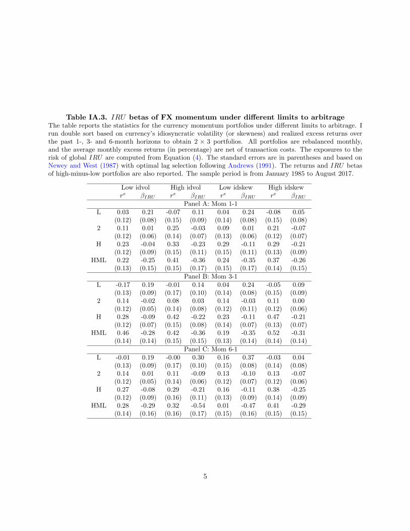
Table IA.3. IRU betas of FX momentum under different limits to arbitrageThe table reports the statistics for the currency momentum portfolios under different limits to arbitrage. Irun double sort based on currency’s idiosyncratic volatility (or skewness) and realized excess returns overthe past 1-, 3- and 6-month horizons to obtain 2 × 3 portfolios. All portfolios are rebalanced monthly,and the average monthly excess returns (in percentage) are net of transaction costs. The exposures to therisk of global IRU are computed from Equation (4). The standard errors are in parentheses and based onNewey and West (1987) with optimal lag selection following Andrews (1991). The returns and IRU betasof high-minus-low portfolios are also reported. The sample period is from January 1985 to August 2017.

Low idvol High idvol Low idskew High idskewre βIRU re βIRU re βIRU re βIRU

Panel A: Mom 1-1L 0.03 0.21 -0.07 0.11 0.04 0.24 -0.08 0.05

(0.12) (0.08) (0.15) (0.09) (0.14) (0.08) (0.15) (0.08)2 0.11 0.01 0.25 -0.03 0.09 0.01 0.21 -0.07

(0.12) (0.06) (0.14) (0.07) (0.13) (0.06) (0.12) (0.07)H 0.23 -0.04 0.33 -0.23 0.29 -0.11 0.29 -0.21

(0.12) (0.09) (0.15) (0.11) (0.15) (0.11) (0.13) (0.09)HML 0.22 -0.25 0.41 -0.36 0.24 -0.35 0.37 -0.26

(0.13) (0.15) (0.15) (0.17) (0.15) (0.17) (0.14) (0.15)Panel B: Mom 3-1

L -0.17 0.19 -0.01 0.14 0.04 0.24 -0.05 0.09(0.13) (0.09) (0.17) (0.10) (0.14) (0.08) (0.15) (0.09)

2 0.14 -0.02 0.08 0.03 0.14 -0.03 0.11 0.00(0.12) (0.05) (0.14) (0.08) (0.12) (0.11) (0.12) (0.06)

H 0.28 -0.09 0.42 -0.22 0.23 -0.11 0.47 -0.21(0.12) (0.07) (0.15) (0.08) (0.14) (0.07) (0.13) (0.07)

HML 0.46 -0.28 0.42 -0.36 0.19 -0.35 0.52 -0.31(0.14) (0.14) (0.15) (0.15) (0.13) (0.14) (0.14) (0.14)

Panel C: Mom 6-1L -0.01 0.19 -0.00 0.30 0.16 0.37 -0.03 0.04

(0.13) (0.09) (0.17) (0.10) (0.15) (0.08) (0.14) (0.08)2 0.14 0.01 0.11 -0.09 0.13 -0.10 0.13 -0.07

(0.12) (0.05) (0.14) (0.06) (0.12) (0.07) (0.12) (0.06)H 0.27 -0.08 0.29 -0.21 0.16 -0.11 0.38 -0.25

(0.12) (0.09) (0.16) (0.11) (0.13) (0.09) (0.14) (0.09)HML 0.28 -0.29 0.32 -0.54 0.01 -0.47 0.41 -0.29

(0.14) (0.16) (0.16) (0.17) (0.15) (0.16) (0.15) (0.15)

5

Table IA.4. Pricing FX momentum under different limits to arbitrageThe table reports the results of asset pricing test for the two-factor model containing the dollar factor andthe global IRU risk factor (uIRU

t ). The testing assets are momentum portfolios within each group of limitsto arbitrage, formed by running double sorts on idiosyncratic volatility (skewness) and realized currencyexcess returns over the past 1-, 3- and 6-month horizons. The test is done via the Fama-MacBeth regression,where I report the estimated risk prices, cross-sectional OLS R2, the heteroskedastic and autocorrelationconsistent (HAC) standard errors based on Newey and West (1987) with optimal lag selection followingAndrews (1991) (NW), and the Shanken-adjusted standard errors of Shanken (1992) (Sh). The p-values ofχ2-test on the null hypothesis that the pricing errors are jointly zero are also reported. The sample periodis from January 1985 to August 2017.

Low idvol High idvol Low idskew High idskewPanel A: Mom 1-1

λDOL λIRU R2 λDOL λIRU R2 λDOL λIRU R2 λDOL λIRU R2

0.17 -0.69 0.63 0.09 -1.06 0.79 0.17 -0.63 0.80 0.03 -1.41 0.88(NW) (0.12) (0.45) (0.11) (0.40) (0.11) (0.39) (0.12) (0.54)(Sh) (0.13) (0.54) (0.12) (0.58) (0.12) (0.46) (0.15) (0.93)χ2NW 2.97 2.22 1.01 2.32

(0.08) (0.14) (0.31) (0.13)χ2Sh 2.00 1.05 0.72 0.78

(0.16) (0.31) (0.40) (0.38)Panel B: Mom 3-1

λDOL λIRU R2 λDOL λIRU R2 λDOL λIRU R2 λDOL λIRU R2

0.14 -1.60 0.98 0.14 -1.17 1.00 0.16 -0.54 0.96 0.11 -1.75 0.99(NW) (0.12) (0.47) (0.11) (0.39) (0.11) (0.37) (0.11) (0.41)(Sh) (0.14) (0.87) (0.12) (0.59) (0.12) (0.42) (0.13) (0.83)χ2NW 0.76 0.01 0.16 0.17

(0.38) (0.90) (0.69) (0.68)χ2Sh 0.21 0.01 0.12 0.04

(0.64) (0.94) (0.72) (0.84)Panel C: Mom 6-1

λDOL λIRU R2 λDOL λIRU R2 λDOL λIRU R2 λDOL λIRU R2

0.21 -0.92 0.92 0.12 -0.49 0.81 0.15 -0.01 -0.27 0.02 -1.46 1.00(NW) (0.12) (0.50) (0.11) (0.29) (0.11) (0.27) (0.12) (0.50)(Sh) (0.13) (0.68) (0.11) (0.33) (0.11) (0.27) (0.15) (0.88)χ2NW 1.05 1.21 0.26 0.00

(0.31) (0.27) (0.61) (0.95)χ2Sh 0.56 0.97 0.26 0.00

(0.45) (0.32) (0.61) (0.97)

6

Figure IA.1. Risk factors when carry or one-month momentum failsThe figure plots the average of innovations to the global interest rate uncertainty, VIX and global FXvolatility when currency carry or momentum strategy experiences sizable losses as defined in Equation (10).The momentum strategy is based on sorting the past one-month realized returns. The sample period is fromJanuary 1985 to August 2017.

<10 <20 <30 <40 <500

0.05

0.1

0.15

0.2

0.25

0.3

0.35

0.4

Inno

vatio

ns to

glo

bal I

RU

CarryMomentum

<10 <20 <30 <40 <50-0.1

0

0.1

0.2

0.3

0.4

0.5

Inno

vatio

ns to

VIX

CarryMomentum

<10 <20 <30 <40 <50-0.1

0

0.1

0.2

0.3

0.4

0.5

0.6

0.7

Inno

vatio

ns to

FX

Vol

CarryMomentum

7

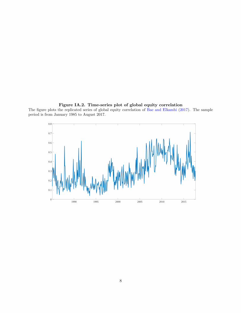
Figure IA.2. Time-series plot of global equity correlationThe figure plots the replicated series of global equity correlation of Bae and Elkamhi (2017). The sampleperiod is from January 1985 to August 2017.

1990 1995 2000 2005 2010 20150

0.1

0.2

0.3

0.4

0.5

0.6

0.7

0.8

8

Figure IA.3. IRU betas under subsamplesThe figure plots the betas of carry and momentum portfolio returns to the global IRU risk, estimated fromEquation (4) by using data from different subsamples. The overall sample period is from January 1985 toAugust 2017.

1 2 3 4 5

-0.4

-0.2

0

0.2

0.4

0.6

0.8

1

1.2Panel A: Carry

Pre-crisisPost-crisisDeveloped economiesExcl.Asian crisisExcl.08 crisisExcl.Euro crisis

1 2 3 4 5

-0.4

-0.2

0

0.2

0.4

0.6

0.8

1

1.2Panel B: Momentum

Pre-crisisPost-crisisDeveloped economiesExcl.Asian crisisExcl.08 crisisExcl.Euro crisis

9