ORIGINAL RESEARCH ARTICLEpublished: 06 January 2014

doi: 10.3389/fnbot.2013.00025

Curiosity driven reinforcement learning for motionplanning on humanoidsMikhail Frank1,2,3*, Jürgen Leitner1,2,3, Marijn Stollenga1,2,3, Alexander Förster1,2,3 and

Jürgen Schmidhuber1,2,3

1 Dalle Molle Institute for Artificial Intelligence, Lugano, Switzerland2 Facoltà di Scienze Informatiche, Università della Svizzera Italiana, Lugano, Switzerland3 Dipartimento Tecnologie Innovative, Scuola Universitaria Professionale della Svizzera Italiana, Manno, Switzerland

Edited by:

Gianluca Baldassarre, ItalianNational Research Council, Italy

Reviewed by:

Anthony F. Morse, University ofSkövde, SwedenHsin Chen, National Tsing-HuaUniversity, TaiwanAlberto Finzi, Università di NapoliFederico II, Italy

*Correspondence:

Mikhail Frank, Dalle Molle Institutefor Artificial Intelligence, Galleria 2,CH-6928 Manno-Lugano,Switzerlande-mail: kail@idsia.ch

Most previous work on artificial curiosity (AC) and intrinsic motivation focuses on basicconcepts and theory. Experimental results are generally limited to toy scenarios, such asnavigation in a simulated maze, or control of a simple mechanical system with one or twodegrees of freedom. To study AC in a more realistic setting, we embody a curious agentin the complex iCub humanoid robot. Our novel reinforcement learning (RL) frameworkconsists of a state-of-the-art, low-level, reactive control layer, which controls the iCubwhile respecting constraints, and a high-level curious agent, which explores the iCub’sstate-action space through information gain maximization, learning a world model fromexperience, controlling the actual iCub hardware in real-time. To the best of our knowledge,this is the first ever embodied, curious agent for real-time motion planning on a humanoid.We demonstrate that it can learn compact Markov models to represent large regions ofthe iCub’s configuration space, and that the iCub explores intelligently, showing interestin its physical constraints as well as in objects it finds in its environment.

Keywords: artificial curiosity, intrinsic motivation, reinforcement learning, humanoid, iCub, embodied AI

1. INTRODUCTIONReinforcement Learning (RL) (Barto et al., 1983; Sutton andBarto, 1998; Kaelbling et al., 1996) allows an agent in an environ-ment to learn a policy to maximize some sort of reward. Ratherthan optimizing the policy directly, many RL algorithms insteadlearn a value function, defined as expected future discountedcumulative reward. Much of early RL research focused on dis-crete states and actions instead of continuous ones dealt with byfunction approximation and feature-based representations.

An RL agents needs to explore its environment. Undirectedexploration methods (Barto et al., 1983), rely on randomlyselected actions, and do not differentiate between alreadyexplored regions and others. Contrastingly, directed explorationmethods can focus the agent’s efforts on novel regions. Theyinclude the classic and often effective optimistic initialization,go-to the least-visited state, and go-to the least recently visitedstate.

1.1. ARTIFICIAL CURIOSITY (AC)Artificial Curiosity (AC) refers to directed exploration driven bya world model-dependent value function designed to direct theagent toward regions where it can learn something. The firstimplementation (Schmidhuber, 1991b) was based on an intrinsicreward inversely proportional to the predictability of the environ-ment. A subsequent AC paper (Schmidhuber, 1991a) emphasizedthat the reward should actually be based on the learning progress,as the previous agent was motivated to fixate on inherentlyunpredictable regions of the environment. Subsequently, a prob-abilistic AC version (Storck et al., 1995) used the well known

Kullback-Leibler (KL) divergence (Lindley, 1956; Fedorov, 1972)to define non-stationary, intrinsic rewards reflecting the changesof a probabilistic model of the environment after new experiences.Itti and Baldi (2005) called this measure Bayesian Surprise anddemonstrated experimentally that it explains certain patterns ofhuman visual attention better than previous approaches.

Over the past decade, robot-oriented applications of curios-ity research have emerged in the closely related fields ofAutonomous Mental Development (AMD) (Weng et al., 2001)and Developmental Robotics (Lungarella et al., 2003). Inspired bychild psychology studies of Piaget (Piaget and Cook, 1952), theyseek to learn a strong base of useful skills, which might be com-bined to solve some externally posed task, or built upon to learnmore complex skills.

Curiosity-driven RL for developmental learning(Schmidhuber, 2006) encourages the learning of appropri-ate skills. Skill learning can be made more explicit by identifyinglearned skills (Barto et al., 2004) within the option frame-work (Sutton et al., 1999). A very general skill learning setting isassumed by the PowerPlay framework, where skills actually corre-spond to arbitrary computational problem solvers (Schmidhuber,2013; Srivastava et al., 2013).

Luciw et al. (2011) built a curious planner with a high-dimensional sensory space. It learns to perceive its worldand predict the consequences of its actions, and continu-ally plans ahead with its imperfect but optimistic model.Mugan and Kuipers developed QLAP (Mugan and Kuipers,2012) to build predictive models on a low-level visuomo-tor space. Curiosity-Driven Modular Incremental Slow Feature

Frontiers in Neurorobotics www.frontiersin.org January 2014 | Volume 7 | Article 25 | 1

NEUROROBOTICS

Frank et al. RL for motion planning

Analysis (Kompella et al., 2012) provides an intrinsic reward foran agent’s progress toward learning new spatiotemporal abstrac-tions of its high-dimensional raw pixel input streams. Learnedabstractions become option-specific feature sets that enable skilllearning.

1.2. DEVELOPMENTAL ROBOTICSDevelopmental Robotics (Lungarella et al., 2003) seeks to enablerobots to learn to do things in a general and adaptive way, by trial-and-error, and it is thus closely related to AMD and the work oncuriosity-driven RL, described in the previous section. However,developmental robotic implementations have been few.

What was possibly the first AC-like implementation to run onhardware (Huang and Weng, 2002) rotated the head of the SAILrobot back and forth. The agent/controller was rewarded based onreconstruction error between its improving internal perceptualmodel and its high-dimensional sensory input.

AC based on learning progress was first applied to a physicalsystem to explore a playroom using a Sony AIBO robotic dog. Thesystem (Oudeyer et al., 2007) selects from a variety of pre-builtbehaviors, rather than performing any kind of low-level con-trol. It also relies on a remarkably high degree of random actionselection, 30%, and only optimizes the immediate (next-step)expected reward, instead of the more general delayed reward.

Model-based RL with curiosity-driven exploration has beenimplemented on a Katana manipulator (Ngo et al., 2012), suchthat the agent learns to build a tower, without explicitly reward-ing any kind of stacking. The implementation does use pre-programmed pick and place motion primitives, as well as a set ofspecialized pre-designed features on the images from an overheadcamera.

A curiosity-driven modular reinforcement learner has recentlybeen applied to surface classification (Pape et al., 2012), usinga robotic finger equipped with an advanced tactile sensor onthe fingertip. The system was able to differentiate distinct tactileevents, while simultaneously learning behaviors (how to move thefinger to cause different kinds of physical interactions between thesensor and the surface) to generate the events.

The so-called hierarchical curiosity loops architec-ture (Gordon and Ahissar, 2011) has recently enabled a 1-DOFLEGO Mindstorms arm to learn simple reaching (Gordon andAhissar, 2012).

Curiosity implementations in developmental robotics havesometimes used high dimensional sensory spaces, but each one,in its own way, greatly simplified the action spaces of the robots byusing pre-programmed high-level motion primitives, discretizingmotor control commands, or just using very, very simple robots.We are unaware of any AC (or other intrinsic motivation) imple-mentation, which is capable of learning in, and taking advantageof a complex robot’s high-dimensional configuration space.

Some methods learn internal models, such as hand-eye motormaps (Nori et al., 2007), inverse kinematic mappings (D’Souzaet al., 2001), and operational space control laws (Peters andSchaal, 2008), but these are not curiosity-driven. Moreover, theylack the generality and robustness of full-blown path planningalgorithms (Latombe et al., 1996; LaValle, 1998; Li and Shie, 2007;Perez et al., 2011).

1.3. THE PATH PLANNING PROBLEMThe Path Planning Problem is to find motions that pursue goalswhile deliberately avoiding arbitrary non-linear constraints, usu-ally obstacles. The ability to solve the path planning problem inpractice is absolutely critical to the eventual goal of deployingcomplex/humanoid robots in unstructured environments. Therecent textbook, “Planning Algorithms” (LaValle, 2006), offersmany interesting approaches to planning motions for complexmanipulators. These are expensive algorithms, which search theconfiguration space to generate trajectories that often requirepost-processing. Thus robots, controlled by algorithmic planners,are typically very deliberate and slow, first “thinking,” often forquite some time, then executing a motion, which would be simpleand intuitive for humans.

1.4. REACTIVE CONTROLIn the 1980s, a control strategy emerged, which was completelydifferent from the established plan first, act later paradigm.The idea was to use potential fields (Khatib, 1986; Kim andKhosla, 1992), and/or dynamical systems (Schoner and Dose,1992; Iossifidis and Schoner, 2004, 2006), and/or the sensor sig-nals directly (Brooks, 1991) to generate control commands fast,without searching the configuration space. Control is based onsome kind of local gradient, which is evaluated at the robot’s cur-rent configuration. As a result, sensors and actuators are tightlycoupled in a fast, light weight action/observation loop, allowinga robot to react quickly and smoothly to changing circumstances.Nevertheless, reactive controllers are shortsighted and prone togetting stuck in local minima/maxima, making them relativelybad path planners.

1.5. A CURIOUS CONFLUENCEIn this paper, we introduce a curiosity-driven reinforcementlearner for the iCub humanoid robot (Metta et al., 2008), whichautonomously learns a powerful, reusable solver of motion plan-ning problems from experience controlling the actual, physicalrobot.

The application of RL to the path planning problem (or moreprecisely the process of embodying the agent at a sufficiently lowlevel of control) has allowed us to incorporate two approaches,planning and reactive control, which for the most part have beentreated separately by roboticists until now. The integrated systembenefits from both approaches while avoiding their most prob-lematic drawbacks, and we believe it to be an important steptoward realizing a practical, feasible, developmental approach toreal, non-trivial robotics problems. Furthermore, the system isnovel in the following ways:

1. In contrast to previous implementations of artificial curiosityand/or intrinsic motivation in the context of developmentalrobotics, our system learns to control many degrees of freedom(DOFs) of a complex robot.

2. Planning algorithms typically generate reference trajectories,which must then be passed to a controller. Our RL system,on the other hand, learns control commands directly, whilestill yielding a resolution complete planner. This greatly sim-plifies many practical issues that arise from tracking a reference

Frontiers in Neurorobotics www.frontiersin.org January 2014 | Volume 7 | Article 25 | 2

Frank et al. RL for motion planning

trajectory and results in a lighter, faster action/observationloop.

3. Rather than relying on reactive control to generate entiremotions, we only use it to implement actions. Thus the com-pleteness of the planner is preserved, although its robustnessis improved by the added capacity of each action react tounforeseen and/or changing constraints.

2. MATERIAL AND METHODSIn order to build a developmental learning system capable ofexploiting the iCub’s high DOF configuration space, we beginby looking at the path planning literature, where there existtwo classes of algorithms, capable of generating high dimen-sional reference trajectories. Single query algorithms, such asRapidly Exploring Random Trees (RRT) (LaValle, 1998; Perezet al., 2011), interpolate two points in configuration space, with-out reusing knowledge from one query to the next. Multiple queryalgorithms on the other hand, such as Probabilistic Road Maps(PRM) (Latombe et al., 1996; Sun et al., 2005), store a compressedrepresentation of the configuration space and satisfy queries byoperating on that data structure, rather than searching the highDOF configuration space directly. In the case of PRM, the config-uration space is represented by a graph, which can even be grownincrementally (Li and Shie, 2007). PRM’s compact, incrementallyexpandable representation of known motions makes it a likelyantecedent to or template for a development learning system,but there are several problems, which are all related to separationbetween planning and control.

To build up a PRM planner, one must first sample the con-figuration space to obtain a set of vertices for the graph. Thesamples are then interpolated by trajectories, which form the setof edges that connect the vertices. The feasibility of each sam-ple (vertex) and trajectory (edge) must be preemptively verified,typically by forward kinematics and collision detection computa-tions, which collectively amount to a computationally expensivepre-processing step. The configuration of the robot must remainon the verified network of samples and trajectories at all times, orthere may be unwanted collisions. This implies that all the trajec-tories in the graph must also be controllable, which is in generaldifficult to verify in simulation for complex robots, such as theiCub, which exhibit non-linear dynamics (due to do friction anddeformation) and are thus very difficult to model faithfully. Ifthese problems can be surmounted, then a PRM planner can beconstructed, however, the configuration of the robot’s workspacemust be static, because moving anything therein may affect thefeasibility of the graph edges.

All of these problems can be avoided by embodying the plan-ner and giving the system the capacity to react. If there were alow-level control system, which could enforce all necessary con-straints (to keep the robot safe and operational) in real time,then the planner could simply try things out, without the need toexhaustively and preemptively verify the feasibility of each poten-tial movement. In this case, reference trajectories would becomeunnecessary, and the planner could simply store, recall, and issuecontrol commands directly. Lastly, and perhaps most importantly,with the capacity to react in real time, there would be no need torequire a static workspace.

This new embodied planner would differ from its antecedentPRM planner in several important ways. There would be noneed to require that the configuration of the robot be on anyof the graph edges. In fact the graph would no longer repre-sent a network of distinct trajectories, but rather the topologyof the continuous configuration space. Each edge would nolonger represent a particular trajectory, but rather a more gen-eral kind of action that implements something like try to goto that region of the configuration space. Such actions would beavailable not when the true robot configuration is on a graphvertex, but rather when it is near that vertex. The actions mayor may not succeed depending on the particular initial configu-ration of the robot when the action was initiated as well as theconfiguration of the workspace, which must not necessarily bestatic.

Allowing the planner to control the hardware directly offersconsiderable benefits, but it also requires a more complex repre-sentation of the configuration space than the plan first, act laterparadigm did. Whereas the PRM planner made do with a sim-ple graph, representing a network of trajectories, the embodiedversion seems to require a probabilistic model, which can copewith actions that may have a number of different outcomes.In light of this requirement, the embodied planner begins tolook like a Markov Decision Process (MDP), and in order toexploit such a planner, the state transition probabilities, whichgovern the MDP, must first be learned. However, this presents aproblem in that experiments (trying out actions) are very expen-sive when run on robotic hardware, which is bound to realtime, as opposed to simulations, which can be run faster thanreal time, or parallelized, or both. Therefore, an efficient explo-ration method is absolutely critical, which motivates our use ofcuriosity-driven RL.

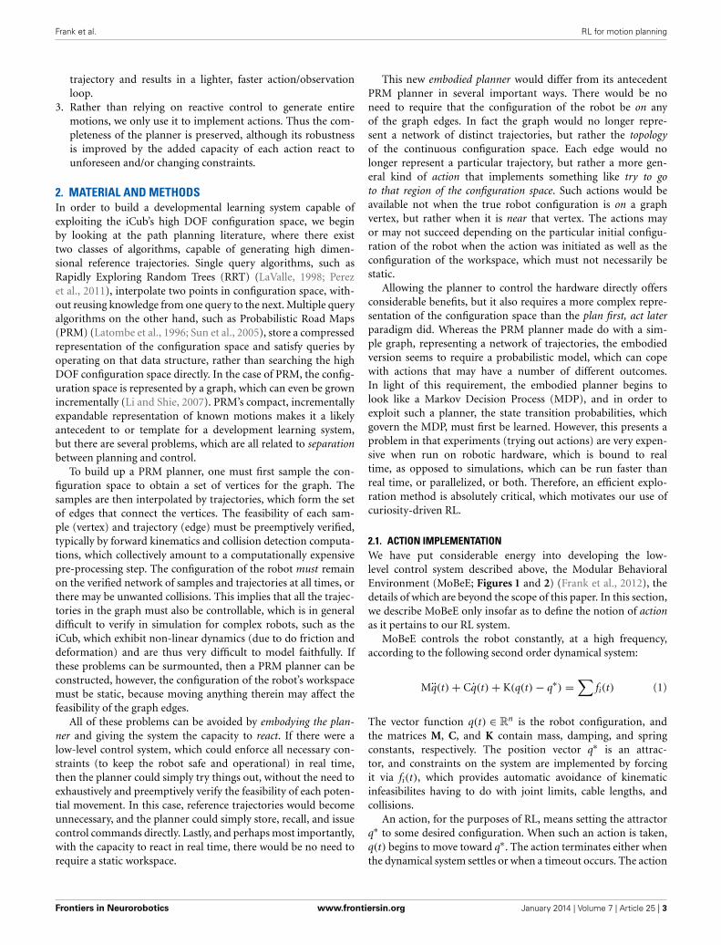
2.1. ACTION IMPLEMENTATIONWe have put considerable energy into developing the low-level control system described above, the Modular BehavioralEnvironment (MoBeE; Figures 1 and 2) (Frank et al., 2012), thedetails of which are beyond the scope of this paper. In this section,we describe MoBeE only insofar as to define the notion of actionas it pertains to our RL system.

MoBeE controls the robot constantly, at a high frequency,according to the following second order dynamical system:

Mq̈(t)+ Cq̇(t)+ K(q(t)− q∗) =∑

fi(t) (1)

The vector function q(t) ∈ Rn is the robot configuration, and

the matrices M, C, and K contain mass, damping, and springconstants, respectively. The position vector q∗ is an attrac-tor, and constraints on the system are implemented by forcingit via fi(t), which provides automatic avoidance of kinematicinfeasibilites having to do with joint limits, cable lengths, andcollisions.

An action, for the purposes of RL, means setting the attractorq∗ to some desired configuration. When such an action is taken,q(t) begins to move toward q∗. The action terminates either whenthe dynamical system settles or when a timeout occurs. The action

Frontiers in Neurorobotics www.frontiersin.org January 2014 | Volume 7 | Article 25 | 3

Frank et al. RL for motion planning

FIGURE 1 | MoBeE and the iCub. MoBeE (left) prevents the iCubhumanoid robot (right) from colliding with the table.Semi-transparent geometries represent force fields, and when these

collide with one another (shown in red), they generate repulsive,constraint forces, which in this case push the hands away fromthe table surface.

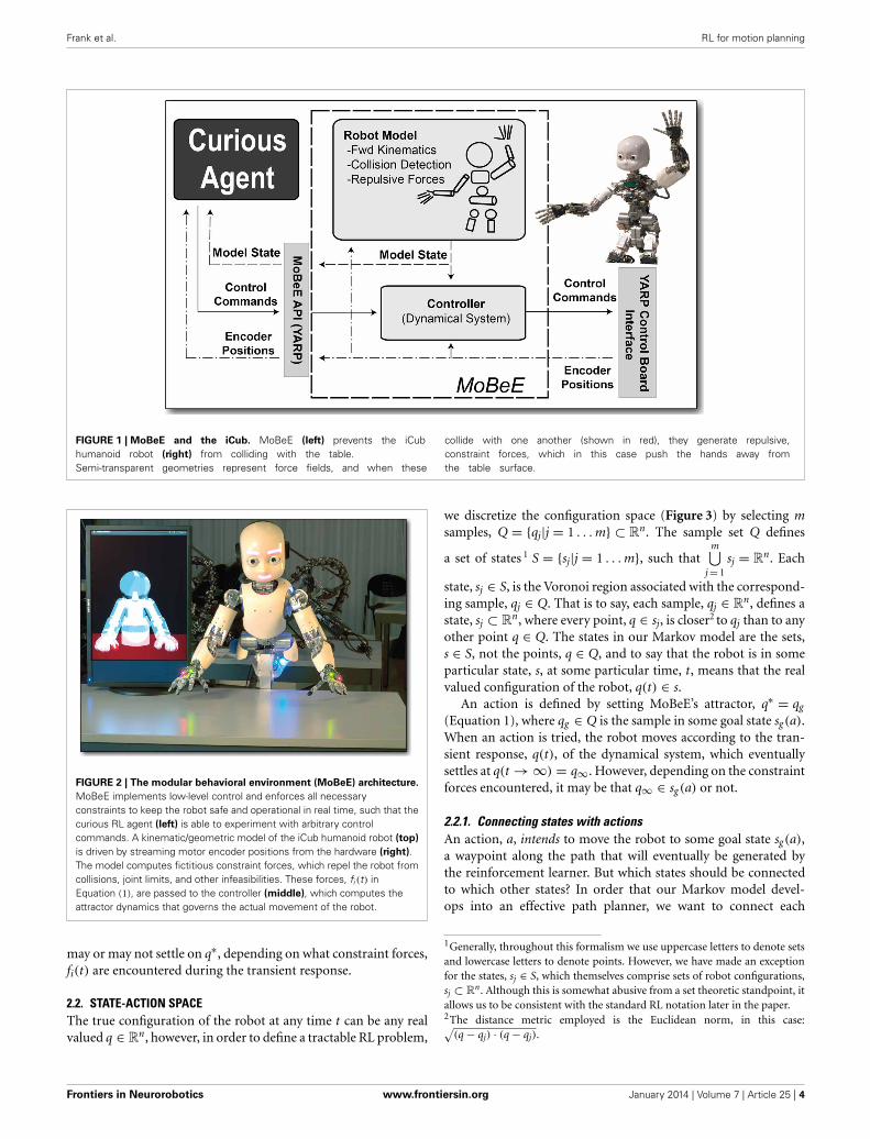
FIGURE 2 | The modular behavioral environment (MoBeE) architecture.

MoBeE implements low-level control and enforces all necessaryconstraints to keep the robot safe and operational in real time, such that thecurious RL agent (left) is able to experiment with arbitrary controlcommands. A kinematic/geometric model of the iCub humanoid robot (top)

is driven by streaming motor encoder positions from the hardware (right).The model computes fictitious constraint forces, which repel the robot fromcollisions, joint limits, and other infeasibilities. These forces, fi (t) inEquation (1), are passed to the controller (middle), which computes theattractor dynamics that governs the actual movement of the robot.

may or may not settle on q∗, depending on what constraint forces,fi(t) are encountered during the transient response.

2.2. STATE-ACTION SPACEThe true configuration of the robot at any time t can be any realvalued q ∈ R

n, however, in order to define a tractable RL problem,

we discretize the configuration space (Figure 3) by selecting msamples, Q = {qj|j = 1 . . . m} ⊂ R

n. The sample set Q defines

a set of states 1 S = {sj|j = 1 . . . m}, such thatm⋃

j= 1sj = R

n. Each

state, sj ∈ S, is the Voronoi region associated with the correspond-ing sample, qj ∈ Q. That is to say, each sample, qj ∈ R

n, defines astate, sj ⊂ R

n, where every point, q ∈ sj, is closer2 to qj than to anyother point q ∈ Q. The states in our Markov model are the sets,s ∈ S, not the points, q ∈ Q, and to say that the robot is in someparticular state, s, at some particular time, t, means that the realvalued configuration of the robot, q(t) ∈ s.

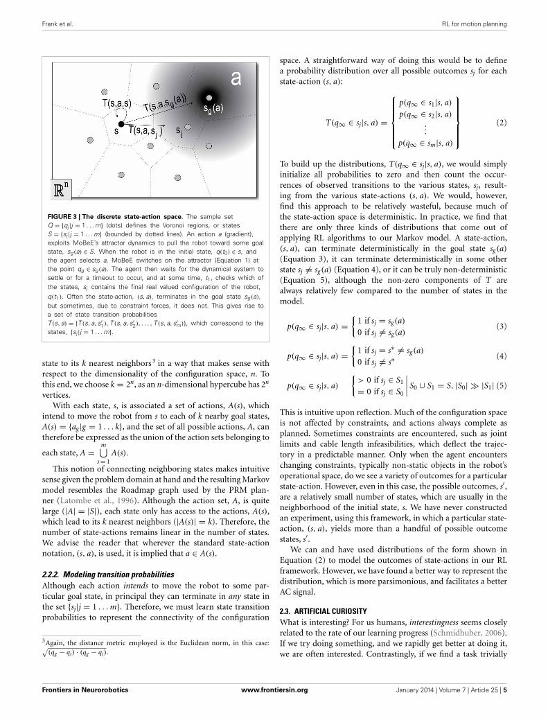
An action is defined by setting MoBeE’s attractor, q∗ = qg

(Equation 1), where qg ∈ Q is the sample in some goal state sg(a).When an action is tried, the robot moves according to the tran-sient response, q(t), of the dynamical system, which eventuallysettles at q(t →∞) = q∞. However, depending on the constraintforces encountered, it may be that q∞ ∈ sg(a) or not.

2.2.1. Connecting states with actionsAn action, a, intends to move the robot to some goal state sg(a),a waypoint along the path that will eventually be generated bythe reinforcement learner. But which states should be connectedto which other states? In order that our Markov model devel-ops into an effective path planner, we want to connect each

1Generally, throughout this formalism we use uppercase letters to denote setsand lowercase letters to denote points. However, we have made an exceptionfor the states, sj ∈ S, which themselves comprise sets of robot configurations,sj ⊂ R

n. Although this is somewhat abusive from a set theoretic standpoint, itallows us to be consistent with the standard RL notation later in the paper.2The distance metric employed is the Euclidean norm, in this case:√

(q− qj) · (q− qj).

Frontiers in Neurorobotics www.frontiersin.org January 2014 | Volume 7 | Article 25 | 4

Frank et al. RL for motion planning

FIGURE 3 | The discrete state-action space. The sample setQ = {qj |j = 1 . . . m} (dots) defines the Voronoi regions, or statesS = {sj |j = 1 . . . m} (bounded by dotted lines). An action a (gradient),exploits MoBeE’s attractor dynamics to pull the robot toward some goalstate, sg(a) ∈ S. When the robot is in the initial state, q(t0) ∈ s, andthe agent selects a, MoBeE switches on the attractor (Equation 1) atthe point qg ∈ sg(a). The agent then waits for the dynamical system tosettle or for a timeout to occur, and at some time, t1, checks which ofthe states, sj contains the final real valued configuration of the robot,q(t1). Often the state-action, (s, a), terminates in the goal state sg(a),but sometimes, due to constraint forces, it does not. This gives rise toa set of state transition probabilitiesT (s, a) = {T (s, a, s′1), T (s, a, s′2), . . . , T (s, a, s′m)}, which correspond to thestates, {sj |j = 1 . . . m}.

state to its k nearest neighbors 3 in a way that makes sense withrespect to the dimensionality of the configuration space, n. Tothis end, we choose k = 2n, as an n-dimensional hypercube has 2n

vertices.With each state, s, is associated a set of actions, A(s), which

intend to move the robot from s to each of k nearby goal states,A(s) = {ag |g = 1 . . . k}, and the set of all possible actions, A, cantherefore be expressed as the union of the action sets belonging to

each state, A =m⋃

s= 1A(s).

This notion of connecting neighboring states makes intuitivesense given the problem domain at hand and the resulting Markovmodel resembles the Roadmap graph used by the PRM plan-ner (Latombe et al., 1996). Although the action set, A, is quitelarge (|A| = |S|), each state only has access to the actions, A(s),which lead to its k nearest neighbors (|A(s)| = k). Therefore, thenumber of state-actions remains linear in the number of states.We advise the reader that wherever the standard state-actionnotation, (s, a), is used, it is implied that a ∈ A(s).

2.2.2. Modeling transition probabilitiesAlthough each action intends to move the robot to some par-ticular goal state, in principal they can terminate in any state inthe set {sj|j = 1 . . . m}. Therefore, we must learn state transitionprobabilities to represent the connectivity of the configuration

3Again, the distance metric employed is the Euclidean norm, in this case:√(qg − qi) · (qg − qi).

space. A straightforward way of doing this would be to definea probability distribution over all possible outcomes sj for eachstate-action (s, a):

T(q∞ ∈ sj|s, a) =

⎧⎪⎪⎪⎪⎨⎪⎪⎪⎪⎩

p(q∞ ∈ s1|s, a)

p(q∞ ∈ s2|s, a)

...

p(q∞ ∈ sm|s, a)

⎫⎪⎪⎪⎪⎬⎪⎪⎪⎪⎭

(2)

To build up the distributions, T(q∞ ∈ sj|s, a), we would simplyinitialize all probabilities to zero and then count the occur-rences of observed transitions to the various states, sj, result-ing from the various state-actions (s, a). We would, however,find this approach to be relatively wasteful, because much ofthe state-action space is deterministic. In practice, we find thatthere are only three kinds of distributions that come out ofapplying RL algorithms to our Markov model. A state-action,(s, a), can terminate deterministically in the goal state sg(a)

(Equation 3), it can terminate deterministically in some otherstate sj �= sg(a) (Equation 4), or it can be truly non-deterministic(Equation 5), although the non-zero components of T arealways relatively few compared to the number of states in themodel.

p(q∞ ∈ sj|s, a) ={

1 if sj = sg(a)

0 if sj �= sg(a)(3)

p(q∞ ∈ sj|s, a) ={

1 if sj = s∗ �= sg(a)

0 if sj �= s∗ (4)

p(q∞ ∈ sj|s, a)

{> 0 if sj ∈ S1

= 0 if sj ∈ S0

∣∣∣∣ S0 ∪ S1 = S, |S0| |S1| (5)

This is intuitive upon reflection. Much of the configuration spaceis not affected by constraints, and actions always complete asplanned. Sometimes constraints are encountered, such as jointlimits and cable length infeasibilities, which deflect the trajec-tory in a predictable manner. Only when the agent encounterschanging constraints, typically non-static objects in the robot’soperational space, do we see a variety of outcomes for a particularstate-action. However, even in this case, the possible outcomes, s′,are a relatively small number of states, which are usually in theneighborhood of the initial state, s. We have never constructedan experiment, using this framework, in which a particular state-action, (s, a), yields more than a handful of possible outcomestates, s′.

We can and have used distributions of the form shown inEquation (2) to model the outcomes of state-actions in our RLframework. However, we have found a better way to represent thedistribution, which is more parsimonious, and facilitates a betterAC signal.

2.3. ARTIFICIAL CURIOSITYWhat is interesting? For us humans, interestingness seems closelyrelated to the rate of our learning progress (Schmidhuber, 2006).If we try doing something, and we rapidly get better at doing it,we are often interested. Contrastingly, if we find a task trivially

Frontiers in Neurorobotics www.frontiersin.org January 2014 | Volume 7 | Article 25 | 5

Frank et al. RL for motion planning

easy, or impossibly difficult, we do not enjoy a high rate of learn-ing progress, and are often bored. We model this phenomenonusing the information theoretic notion of information gain, or KLdivergence.

2.3.1. KL divergenceKL Divergence, DKL is defined as follows, where Pj and Tj are thescalar components of the discrete probability distributions P andT, respectively.

DKL(P||T) =∑

j

ln

(Pj

Tj

)Pj (6)

For our purposes, T represents the estimated state transitionprobability distribution (Equation 2) for a particular state-action,(s, a), after the agent has accumulated some amount of experi-ence. Once the agent tries (s, a) again, an s′ is observed, and thestate transition probability distribution for (s, a) is updated. Thisnew distribution, P, is a better estimate of the state transitionprobabilities for (s, a), as it is based on more data.

By computing DKL(P||T), we can measure how much ourMarkov model improved by trying the state-action, (s, a), and wecan use this information gain to reward our curious agent. Thus,the agent is motivated to improve its model of the state-actionspace, and it will gravitate toward regions thereof, where learningis progressing quickly.

There is, however, a problem. The KL divergence is not definedif there exist components of P or T, which are equal to zero. Thisis somewhat inconvenient in light of the fact that for our appli-cation, most of the components of most of the distributions, T(Equation 2), are actually zero. We must therefore initialize P andT cleverly.

Perhaps the most obvious solution would be to initialize Twith a uniform distribution, before trying some action for the firsttime. After observing the outcome of the selected action, P wouldbe defined and DKL(P||T) computed, yielding the interestingnessof the action taken.

Some examples of this kind of initialization are given inEquations (7–10) 4. Clearly the approach solves the numericalproblem with the zeros, but it means that initially, every actionthe agent tries will be equally interesting. Moreover, how inter-esting those first actions are, |DKL(P||T)|, depends on the size ofthe state space.

DKL({1, 2, 1} || {1, 1, 1}) = 0.0589 (7)

DKL({2, 1, 1} || {1, 1, 1}) = 0.0589 (8)

DKL({1, 1, 2, 1, 1} || {1, 1, 1, 1, 1}) = 0.0487 (9)

DKL({1, 1, 1, 2, 1, 1, 1} || {1, 1, 1, 1, 1, 1, 1}) = 0.0398 (10)

The first two examples, Equations (7), (8), show that regardlessof the outcome, all actions generate the same numerical inter-estingness the first time they are tried. While not a problem in

4We have intentionally not normalized P and T, to show how they are gen-erated by counting observations of q∞ ∈ sj. In order to actually computeDKL(P||T), P and T must first be normalized.

Algorithm 1: Observe(s,a,s′,T(s, a),R(s, a))

beginif there is no bin, Ts′(s, a), in T(s, a) to count occurrencesof s′ then

append a bin, Ts′(s, a) to T(s, a)

Ts′(s, a)← 1endP← T(s, a)

Ps′ ← Ps′ + 1R(s, a)← DKL(P||T(s, a))

T(s, a)← Pend

theory, in practice this means our robot will need many triesto gather enough information to differentiate the boring, deter-ministic states from the interesting, non-deterministic ones. Sinceour actions are designed to take the agent to a goal state, sg(a),it would be intuitive if observing a transition to sg(a) were lessinteresting than observing one to some other state. This woulddrastically speed up the learning process.

The second two examples, Equations (9), (10) show that theinterestingness of that first try decreases in larger state spaces, oralternatively, small state spaces are numerically more interestingthan large ones. This is not a problem if there is only one learneroperating in a single state-action space. However, in the case ofa multi-agent system, say one learner per body part, it would beconvenient if the intrinsic rewards gotten by the different agentswere numerically comparable to one another, regardless of therelative sizes of those learners’ state-action spaces.

In summary, we have two potential problems with KLDivergence as a reward signal:

1. Slowness of initial learning2. Sensitivity to the cardinality of the distributions

Nevertheless, in many ways, KL Divergence captures exactly whatwe would like our curious agent to focus on. It turns out we canaddress both of these problems by representing T with an array ofvariable size, and initializing the distribution optimistically withrespect to the expected behavior of the action (s, a).

2.3.2. Dynamic state transition distributionsBy compressing the distributions T and P, i.e., not explicitly rep-resenting any bins that contain a zero, we can compute the KLdivergence between only their non-zero components. The processbegins with T and P having no bins at all. However, they grow incardinality as follows: Every time we observe a novel s′ as the resultof trying a state-action (s, a), we append a new bin to the distribu-tion T(s, a), and initialize it with a 1, and copy it to yield P(s, a).Then, since we just observed (s, a) result in s′, we increment thecorresponding bin in P(s, a), and compute KL(P||T). This processis formalized in Algorithm 1.

The optimistic initialization is straightforward. Initially, thedistribution T(s, a) is empty. Then we observe (Algorithm 1)that (s, a) fails, leaving the agent in the initial state, s. The KLdivergence between the trivial distributions {1} and {2} is 0, and

Frontiers in Neurorobotics www.frontiersin.org January 2014 | Volume 7 | Article 25 | 6

Frank et al. RL for motion planning

therefore, so is the reward, R(s, a). Next, we observe that (s, a)

succeeds, moving the agent to the intended goal state, sg(a).The distribution, T(s, a), becomes non-trivial, a non-zero KLdivergence is computed, and thus R(s, a) gets an optimisticallyinitialized reward, which does not depend on the size of the state-action space. Algorithm 2 describes the steps of this optimisticinitialization, and Table 1 shows how T(s, a) and R(s, a) developthroughout the initialization process.

The distributions T, as initialized above, are compact andparsimonious, and they faithfully represent the most likely out-comes of the actions. Moreover, the second initialization stepyields a non-zero KL Divergence, which is not sensitive to the

Algorithm 2: Curious_Explore(S,A,T,R,γ,δ)

beginfor each state-action (s ∈ S, a ∈ A(s)) do

Observe(s, a, s, T(s, a), R(s, a))

Observe(s, a, sg(a), T(s, a), R(s, a))

endwhile true do

Value_Iteration(S, A, T, R, γ, δ)

s← sj|q(tbefore) ∈ sj

agreedy ← a |V(s, a) = argmax({V(s, a)|a ∈ A(s)})run agreedy on the robots′ ← sj|q(tafter) ∈ sj

Observe(s, a, s′, T(s, a), R(s, a))

endend

Algorithm 3: Value_Iteration(S,A,T,R,γ,δ)

beginfor each state-action (s ∈ S, a ∈ A(s)) do

V(s, a)← 0.0endfor each state s ∈ S do

V(s)← 0.0endwhile true do

max_delta← 0.0for each state-action (s ∈ S, a ∈ A(s)) do

Vnew(s, a)← R(s, a)+ γ∑

s′ T(s, a, s′)V(s′)if Vnew(s, a)− V(s, a) > max_delta then

max_delta← Vnew(s, a)− V(s, a)

endV(s, a)← Vnew(s, a)

endfor each state s ∈ S do

V(s)← argmax({V(s, a)|i = s})endif max_delta < δ then

breakend

endend

size of the state space. Importantly, the fact that our initial-ization of the state transition probabilities provides an initialmeasure of interestingness for each state-action allows us, withoutchoosing parameters, to optimistically initialize the reward matrixwith well defined intrinsic rewards. Consequently, we can employa greedy policy, and aggressively explore the state-action spacewhile focusing extra attention on the most interesting regions.As the curious agent explores, the intrinsic rewards decay in alogical way. A state-action, which deterministically leads to itsgoal state (Table 2) is less interesting over time than a state-action that leads to some other state (Table 3), and of coursemost interesting are state-actions with more possible outcomes(Table 4).

2.4. REINFORCEMENT LEARNINGAt the beginning of section 2, we made the claim that a PRMplanner’s compact, incrementally expandable representation ofknown motions makes it a likely antecedent to a developmen-tal learning system. Furthermore, we observed that many of the

Table 1 | Initialization of state transition probabilities.

Observation T P R = DKL(P||T)

– {} {} –

si {1} {2} 0

sg(a) {2,1} {2,2} 0.0589

Table 2 | A predictable action ends in the predicted state.

Observation T P R = DKL(P||T)

init {2,1} {2,2} 0.0589

sg(a) {2,2} {2,3} 0.0201

sg(a) {2,3} {2,4} 0.0095

sg(a) {2,4} {2,5} 0.0052

Table 3 | A predictable action ends in a surprising state.

Observation T P R = DKL(P||T)

init {2,1} {2,2} 0.0589

sj {2,2,1} {2,2,2} 0.0487

sj {2,2,2} {2,2,3} 0.0196

sj {2,2,3} {2,2,4} 0.0103

Table 4 | An unpredictable action.

Observation T P R = DKL(P||T)

init {2,1} {2,2} 0.0589

sa {2,2,1} {2,2,2} 0.0487

sb {2,2,2,1} {2,2,2,2} 0.0345

sc {2,2,2,2,1} {2,2,2,2,2} 0.0283

sg(a) {2,2,2,2,2} {2,3,2,2,2} 0.0142

sa {2,3,2,2,2} {2,3,3,2,2} 0.0133

sb {2,3,3,2,2} {2,3,3,3,2} 0.0125

Frontiers in Neurorobotics www.frontiersin.org January 2014 | Volume 7 | Article 25 | 7

Frank et al. RL for motion planning

weaknesses of PRMs can be avoided by embodying the plannerand coupling it to a low-level reactive controller. Proxied by thislow-level controller, the planner is empowered to try out arbitrarycontrol signals, however, it does not necessarily know what willhappen. Therefore, the PRM’s original model of the robot’s state-action space, a simple graph, is insufficient, and a more powerful,probabilistic model, an MDP is required. Thus, modeling therobot-workspace system using an MDP arises naturally from theeffort to improve the robustness of a PRM planner, and accord-ingly, Model-Based RL is the most appropriate class of learningalgorithms to operate on the MDP.

Having specified what action means in terms of robot control(section 2.1), described the layout and meaning of the state-action space (section 2.2), and defined the way in which intrinsicreward is computed according to the AC principal (section 2.3),we are ready to incorporate these pieces in a Model-Based RL sys-tem, which develop into a path planner as follows: Initially, setsof states and actions will be chosen, according to some heuris-tic(s), such that the robot’s configuration space is reasonably wellcovered and the RL computations are tractable. Then, the statetransition probabilities will be learned for each state-action pair,as the agent explores the MDP by moving the robot about. Thisexploration for the purposes of model learning will be guidedentirely by the intrinsic reward defined in section 2.3, and thecurious agent will continually improve its model of the iCub andits configuration space. In order to exploit the planner, an exter-nal reward must be introduced, which can either be added to orreplace the intrinsic reward function.

The MDP, which constitutes the path planner, is a tuple,< S, A, T, R, γ >, where S is a finite set of m states, A is a finiteset of actions, T is a set of state transition probability distribu-tions, R is a reward function, and γ is a discount factor, whichrepresents the importance of future rewards. This MDP is some-what unusual in that not all of the actions a ∈ A are availablein every state s ∈ S. Therefore, we define sets, A(s), which com-prise the actions a ∈ A that are available to the agent when it

finds itself in state s, and A =m⋃

s= 1A(s). The set of state transition

probabilities becomes T :m⋃

s= 1A(s)× S→ [0, 1], and in general,

the reward function becomes R :m⋃

s= 1A(s)× S→ R, although

the intrinsic reward, Rintrinsic :m⋃

s= 1A(s)→ R, varies only with

state-action pairs (s, a), as opposed to state-action-state triples(s, a, s′). The state transition probabilities, T, are learned bycurious exploration (Algorithm 2, γ = 0.9, δ = 0.001), the RLalgorithm employed is value iteration (Algorithm 3), and theintrinsic reward is computed as shown in Algorithm 1.

3. RESULTSHere we present the results of two online learning experiments.The first one learns a motion planner for a single limb, the iCub’sarm, operating in an unobstructed workspace, while other bodyparts remain motionless. The planner must contend with self-collisions, and infeasibilities due to the relative lengths of thecables, which move the shoulder joints. These constraints are

static, in that they represent properties of the robot itself, whichdo not change regardless of the configuration of the workspace.Due to the static environment, a PRM planner would in prin-cipal be applicable, and the experiment provides a context inwhich to compare and contrast the PRM versus MDP planners.Still, the primary question addressed by this first experimentis: “To what extent does AC help the agent learn the statetransition probabilities for the MDP planner in this real-worldsetting?”

In the second experiment, the iCub is positioned at a worktable, which constitutes a large obstacle in its workspace. Threecurious agents, unaware of one another’s states, learn planners forthe iCub’s torso and two arms, respectively. One could in princi-pal define a single curious MDP planner for the whole body, butthis would result in an explosion of the state-action space suchthat running actual experiments on the iCub hardware would beprohibitively time consuming. The modular, parallel, multi-agentconfiguration of this second experiment is designed to addressthe question: “Can curious MDP planners scale to intelligentlycontrol the entire iCub robot?” And in observing the behavioremergent from the interactions between the 3 learners, this willbe the question of primary importance. Also noteworthy, how-ever, is that from the perspective of the arms, which do notknow that the torso is moving, the table seems to be non-static.By analyzing the arm learning while disregarding the torso, onecan gain insight into how the curious MDP planner copes withnon-static environments, which would render the PRM plannerinoperable.

3.1. PLANNING IN A STATIC ENVIRONMENT—LEARNING TO AVOIDSELF-COLLISIONS AND CABLE LENGTH INFEASIBILITIES

In the first experiment, “Planning in a static environment,” wecompare the exploration of our artificially curious agent (AC),to two other agents using benchmark exploration strategies fromthe RL literature. One explores randomly (RAND), and the otheralways selects the state-action least tried (LT)5.

The state space is defined by choosing samples, which varyin 4 dimensions corresponding to three shoulder joints and theelbow. Each of these joints is sampled at 25%, 50%, and 75%of its range of motion, resulting in a 4D hyper-lattice with 81vertices, which are connected to their 24 = 16 nearest neighborsas per section 2.2.1, yielding 81× 16 = 1296 state-actions. Theintuition behind this choice of state space it comprises a compactyet reasonably well dispersed set of pre-reach poses.

The task is to find the infeasible region(s) of the configura-tion space, and learn the according state transition probabilitiessuch that the agent can plan motions effectively. The task is rel-atively simple, but it is none the less a crucial aspect of anypath planning that should take place on the iCub. Without delib-erately avoiding self-collisions and cable length infeasibilities,a controller can and will break the iCub’s cables, rendering itinoperable.

In comparing the AC agent with the RAND agent and theLT agent, we find that AC produces, by far, the best explorer

5If there are multiple least-tried state-actions (for example when none havebeen tried), a random one from the least tried set is selected.

Frontiers in Neurorobotics www.frontiersin.org January 2014 | Volume 7 | Article 25 | 8

Frank et al. RL for motion planning

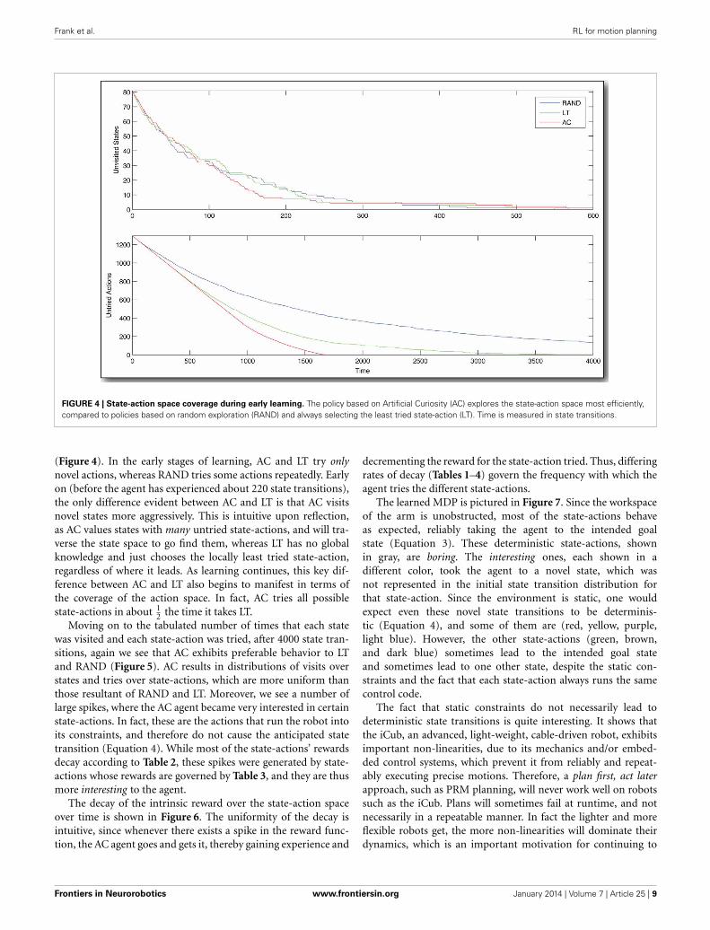
FIGURE 4 | State-action space coverage during early learning. The policy based on Artificial Curiosity (AC) explores the state-action space most efficiently,compared to policies based on random exploration (RAND) and always selecting the least tried state-action (LT). Time is measured in state transitions.

(Figure 4). In the early stages of learning, AC and LT try onlynovel actions, whereas RAND tries some actions repeatedly. Earlyon (before the agent has experienced about 220 state transitions),the only difference evident between AC and LT is that AC visitsnovel states more aggressively. This is intuitive upon reflection,as AC values states with many untried state-actions, and will tra-verse the state space to go find them, whereas LT has no globalknowledge and just chooses the locally least tried state-action,regardless of where it leads. As learning continues, this key dif-ference between AC and LT also begins to manifest in terms ofthe coverage of the action space. In fact, AC tries all possiblestate-actions in about 1

2 the time it takes LT.Moving on to the tabulated number of times that each state

was visited and each state-action was tried, after 4000 state tran-sitions, again we see that AC exhibits preferable behavior to LTand RAND (Figure 5). AC results in distributions of visits overstates and tries over state-actions, which are more uniform thanthose resultant of RAND and LT. Moreover, we see a number oflarge spikes, where the AC agent became very interested in certainstate-actions. In fact, these are the actions that run the robot intoits constraints, and therefore do not cause the anticipated statetransition (Equation 4). While most of the state-actions’ rewardsdecay according to Table 2, these spikes were generated by state-actions whose rewards are governed by Table 3, and they are thusmore interesting to the agent.

The decay of the intrinsic reward over the state-action spaceover time is shown in Figure 6. The uniformity of the decay isintuitive, since whenever there exists a spike in the reward func-tion, the AC agent goes and gets it, thereby gaining experience and

decrementing the reward for the state-action tried. Thus, differingrates of decay (Tables 1–4) govern the frequency with which theagent tries the different state-actions.

The learned MDP is pictured in Figure 7. Since the workspaceof the arm is unobstructed, most of the state-actions behaveas expected, reliably taking the agent to the intended goalstate (Equation 3). These deterministic state-actions, shownin gray, are boring. The interesting ones, each shown in adifferent color, took the agent to a novel state, which wasnot represented in the initial state transition distribution forthat state-action. Since the environment is static, one wouldexpect even these novel state transitions to be determinis-tic (Equation 4), and some of them are (red, yellow, purple,light blue). However, the other state-actions (green, brown,and dark blue) sometimes lead to the intended goal stateand sometimes lead to one other state, despite the static con-straints and the fact that each state-action always runs the samecontrol code.

The fact that static constraints do not necessarily lead todeterministic state transitions is quite interesting. It shows thatthe iCub, an advanced, light-weight, cable-driven robot, exhibitsimportant non-linearities, due to its mechanics and/or embed-ded control systems, which prevent it from reliably and repeat-ably executing precise motions. Therefore, a plan first, act laterapproach, such as PRM planning, will never work well on robotssuch as the iCub. Plans will sometimes fail at runtime, and notnecessarily in a repeatable manner. In fact the lighter and moreflexible robots get, the more non-linearities will dominate theirdynamics, which is an important motivation for continuing to

Frontiers in Neurorobotics www.frontiersin.org January 2014 | Volume 7 | Article 25 | 9

Frank et al. RL for motion planning

FIGURE 5 | Distributions of visits over states and tries over

actions. Our curious agent (AC) visits states and tries actions in amore uniformly than to policies based on random exploration (RAND)and always selecting the least tried state-action (LT). Note the fewstate-actions, which have been tried many times by AC. These are

affected by the cable length constraints in the iCub’s shoulder. Theyterminate in an unexpected way, which is interesting or surprising tothe agent, and they therefore receive more attention. These data arecompiled over 4000 state transitions, observed while controlling thereal, physical iCub humanoid robot.

develop more robust solutions, such as the MDP motion planningpresented here.

3.2. DISCOVERING THE TABLE WITH A MULTI-AGENT RL SYSTEMIn the second experiment, we control both of the iCub’s arms andits torso, 12 DOF in total. A hypercube in 12 dimensions has 4096vertices, and a rank 3 hyper-lattice has 531,441 vertices. Clearly,uniform sampling in 12 dimensions will not yield a feasible RLproblem. Therefore, we have parallelized the problem, employingthree curious agents that control each arm and the torso sepa-rately, not having access to one another’s state. The state-actionspaces for the arms are exactly as described in the previous exper-iment, and the state-action space for the 3D torso is defined inan analogous manner (25%, 50%, and 75% of each joint’s rangeof motion), resulting in a 3D lattice with 27 vertices, which areconnected to their 23 = 8 nearest neighbors as per section 2.2.1,yielding 27× 8 = 216 state-actions.

We place the iCub in front of a work table, and all three learn-ers begin exploring (Figure 8). The three agents operate strictlyin parallel, having no access to any state information from theothers, however, they are loosely coupled through their effectson the robot. For example, the operational space position of thehand (and therefore whether or not it is colliding with the table)

depends not only on the positions of the joints in the arm, butalso on the positions of the joints in the torso. Thus, we havethree interacting POMDPs, each of which has access to a differentpiece of the complete robot state, and the most interesting parts ofthe state-action spaces are where the state of one POMDP affectssome state transition(s) of another.

When the torso is upright, each arm can reach all of the statesin its state space, but when the iCub is bent over at the waist,the shoulders are much closer to the table, and some of thearms’ state-actions become infeasible, because the robot’s handshit the table. Such interactions between the learners producestate-transition distributions, like the one shown in Figure 9,which are much richer than those from the previous experiment.Moreover these state-actions are the most interesting becausethey generate the most slowly decaying intrinsic reward of thetype shown in Table 4. The result is that the arms learn to avoidconstraints as in the first experiment, but over time, anotherbehavior emerges. The iCub becomes interested in the table, andbegins to touch it frequently. Throughout the learning process,it spends periods of time exploring, investigating its static armconstraints, and touching the table, in a cyclic manner, as allthe intrinsic rewards decay over time in a manner similar toFigure 6.

Frontiers in Neurorobotics www.frontiersin.org January 2014 | Volume 7 | Article 25 | 10

Frank et al. RL for motion planning

FIGURE 6 | Decay of intrinsic reward over time. These snapshots of the reward distribution state-actions (x-axis) over time (from top to bottom) show howour curious agent becomes bored as it builds a better and better model of the state-action space. Time is measured in state transitions.

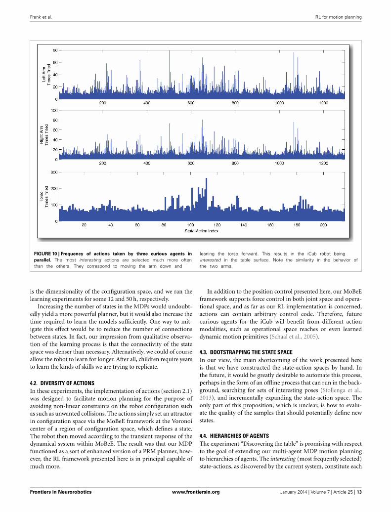
In Figure 10, we have tabulated the distribution of tries overthe state-action space for each of the three learners after 18,000state transitions, or a little more than two full days of learning.As in the previous experiment, we see that the curious agentprefers certain state-actions, selecting them often. Observing thebehavior of the robot during the learning process, it is clear thatthese frequently chosen state-actions correspond to putting thearm down low, and leaning forward, which result in the iCub’shand interacting with the table. Furthermore, the distributionof selected state-actions for the right arm and the left arm arevery similar indeed. This is to be expected, since the arms aremechanically very similar and their configuration spaces havebeen discretized the same way. It is an encouraging result, whichseems to indicate that the variation in the number of times dif-ferent state-actions are selected does indeed capture the extent towhich those state-actions interfere with (or are interfered with by)the other learners.

The emergence of the table exploration behavior is quitepromising with respect to the ultimate goal of using MDP basedmotion planning to control an entire humanoid intelligently. Wepartitioned an intractable configuration space into several looselycoupled RL problems, and with only intrinsic rewards to guidetheir exploration, the learning modules coordinated their behav-ior, causing the iCub to explore the surface of the work table

in front of it. Although the state spaces were generated using acoarse uniform sampling, and the object being explored was largeand quite simple, the experiment nevertheless demonstrates thatMDP motion planning with AC can empower a humanoid robotwith many DOF to explore its environment in a structured wayand build useful, reusable models.

3.2.1. Planning in a dynamic environmentThere is an alternative way to view the multi-agent experiment.Because the arm does not have access to the torso’s state, theexperiment is exactly analogous to one in which the arm is theonly learner and the table is a dynamic obstacle, moving about asthe arm learns. Even from this alternative viewpoint, it is none theless true that some actions will have different outcomes, depend-ing on the table configuration, and will result in state transitiondistributions like the one shown in Figure 9. The key thing toobserve here is that if we were to exploit the planner by placing anexternal reward at some goal, removing the intrinsic rewards, andrecomputing the value function, then the resulting policy/planwill try to avoid the unpredictable regions of the state-actionspace, where state transition probabilities are relatively low. Inother words, training an MDP planner in an environment withdynamic obstacles, will produce policies that plan around regionswhere there tend to be obstacles.

Frontiers in Neurorobotics www.frontiersin.org January 2014 | Volume 7 | Article 25 | 11

Frank et al. RL for motion planning

FIGURE 7 | The learned single-arm MDP planner. The 4D statespace is labeled as follows: shoulder flexion/extension (1,2,3), armabduction/adduction (a,b,c), lateral/medial arm rotation (I,II,III), elbowflexion/extension (A,B,C). Each color represents an interestingstate-action, which often takes the agent to some unexpected state.Each arrow of a particular color represents a state transitionprobability and the weight of the arrow is proportional to themagnitude of that probability. Arrows in gray represent boringstate-actions. These work as expected, reliably taking the agent tothe intended goal state, to which they point.

FIGURE 8 | Autonomous exploration. This composite consists of imagestaken every 30 s or so over the first hour of the experiment described insection 3.2.1. Although learning has just begun, we already begin to seethat the cloud of robot poses is densest (most opaque) near the table. Notethat the compositing technique as well as the wide angle lens used herecreate the illusion that the hands and arms are farther from the table thanthey really are. In fact, the low arm poses put the hand or the elbow within2 cm of the table, as shown in Figure 8.

4. DISCUSSIONIn this paper we have developed an embodied, curious agent, andpresented the first experiments we are aware of, which exploitAC to learn an MDP based motion planner for a real, physical

FIGURE 9 | State space and transition distribution for an interesting

arm action in multi-agent system. The 4D state space is labeled asfollows: shoulder flexion/extension (1,2,3), arm abduction/adduction (a,b,c),lateral/medial arm rotation (I,II,III), elbow flexion/extension (A,B,C). The redarrows show the distribution of next states resultant of an interestingstate-action, which causes the hand to interact with the table. Each arrowrepresents a state transition probability and the weight of the arrow isproportional to the magnitude of that probability. Arrows in gray representboring state-actions. These work as expected, reliably taking the agent tothe intended goal state, to which they point.

humanoid robot. We demonstrated the efficacy of the AC conceptwith a simple learning experiment wherein one learner controlsone of the iCub humanoid’s arms. The primary result of this firstexperiment was that the iCub’s autonomous exploratory behav-ior, guided by AC, efficiently generated a continually improvingMarkov model, which can be (re)used at any time to quicklysatisfy path planning queries.

Furthermore, we conducted a second experiment, in whichthe iCub was situated at a work table while three curious agentscontrolled the its arms and torso, respectively. Acting in parallel,the three agents had no access to one another’s state, however,the interaction between the three learners produced an inter-esting emergent behavior; guided only by intrinsic rewards, thetorso and arm coordinated their movements such that the iCubexplored the surface of the table.

4.1. SCALABILITYFrom the standpoint of scalability, the state spaces used for thearms and torso were more than tractable. In fact the time it tookthe robot to move from one pose/state to another exceeded thetime it took to update the value function by approximately anorder of magnitude. From an experimental standpoint, the limit-ing factor with respect to the size of the state-action space was thetime it took to try all the state-actions a few times. In these exper-iments we connected states to their 2n nearest neighbors, where n

Frontiers in Neurorobotics www.frontiersin.org January 2014 | Volume 7 | Article 25 | 12

Frank et al. RL for motion planning

FIGURE 10 | Frequency of actions taken by three curious agents in

parallel. The most interesting actions are selected much more oftenthan the others. They correspond to moving the arm down and

leaning the torso forward. This results in the iCub robot beinginterested in the table surface. Note the similarity in the behavior ofthe two arms.

is the dimensionality of the configuration space, and we ran thelearning experiments for some 12 and 50 h, respectively.

Increasing the number of states in the MDPs would undoubt-edly yield a more powerful planner, but it would also increase thetime required to learn the models sufficiently. One way to mit-igate this effect would be to reduce the number of connectionsbetween states. In fact, our impression from qualitative observa-tion of the learning process is that the connectivity of the statespace was denser than necessary. Alternatively, we could of courseallow the robot to learn for longer. After all, children require yearsto learn the kinds of skills we are trying to replicate.

4.2. DIVERSITY OF ACTIONSIn these experiments, the implementation of actions (section 2.1)was designed to facilitate motion planning for the purpose ofavoiding non-linear constraints on the robot configuration suchas such as unwanted collisions. The actions simply set an attractorin configuration space via the MoBeE framework at the Voronoicenter of a region of configuration space, which defines a state.The robot then moved according to the transient response of thedynamical system within MoBeE. The result was that our MDPfunctioned as a sort of enhanced version of a PRM planner, how-ever, the RL framework presented here is in principal capable ofmuch more.

In addition to the position control presented here, our MoBeEframework supports force control in both joint space and opera-tional space, and as far as our RL implementation is concerned,actions can contain arbitrary control code. Therefore, futurecurious agents for the iCub will benefit from different actionmodalities, such as operational space reaches or even learneddynamic motion primitives (Schaal et al., 2005).

4.3. BOOTSTRAPPING THE STATE SPACEIn our view, the main shortcoming of the work presented hereis that we have constructed the state-action spaces by hand. Inthe future, it would be greatly desirable to automate this process,perhaps in the form of an offline process that can run in the back-ground, searching for sets of interesting poses (Stollenga et al.,2013), and incrementally expanding the state-action space. Theonly part of this proposition, which is unclear, is how to evalu-ate the quality of the samples that should potentially define newstates.

4.4. HIERARCHIES OF AGENTSThe experiment “Discovering the table” is promising with respectto the goal of extending our multi-agent MDP motion planningto hierarchies of agents. The interesting (most frequently selected)state-actions, as discovered by the current system, constitute each

Frontiers in Neurorobotics www.frontiersin.org January 2014 | Volume 7 | Article 25 | 13

Frank et al. RL for motion planning

agent’s ability to interact with the others. Therefore they areexactly the actions that should be considered by a parent agent,whose job it would be to coordinate the different body parts. Itis our strong suspicion that all state-actions, which are not inter-esting to the current system, can be compressed as “irrelevant” inthe eyes of such a hypothetical parent agent. However, to developthe particulars of the communication up and down the hierarchyremains a difficult challenge, and the topic of ongoing work.

ACKNOWLEDGMENTSThe authors would like to thank Jan Koutnik, Matt Luciw, TobiasGlasmachers, Simon Harding, Gregor Kaufmann, and Leo Pape,for their collaboration, and their contributions to this project.

FUNDINGThis research was supported by the EU Project IM-CLeVeR,contract no. FP7-IST-IP-231722.

REFERENCESBarto, A. G., Singh, S., and Chentanez, N. (2004). “Intrinsically motivated learn-

ing of hierarchical collections of skills,” in Proceedings of the 3rd InternationalConference Development Learning (San Diego, CA), 112–119.

Barto, A. G., Sutton, R. S., and Anderson, C. W. (1983). Neuronlike adaptive ele-ments that can solve difficult learning control problems. IEEE Trans. Syst. ManCybern. SMC-13, 834–846. doi:10.1109/TSMC.1983.6313077

Brooks, R. (1991). Intelligence without representation. Artif. Intell. 47, 139–159.doi: 10.1016/0004-3702(91)90053-M

D’Souza, A., Vijayakumar, S., and Schaal, S. (2001). Learning inverse kinematics.Int. Conf. Intell. Robots Syst. 1, 298–303. doi: 10.1109/IROS.2001.973374

Fedorov, V. V. (1972). Theory of Optimal Experiments. New York, NY: AcademicPress.

Frank, M., Leitner, J., Stollenga, M., Kaufmann, G., Harding, S., Forster, A., et al.(2012). “The modular behavioral environment for humanoids and other robots(mobee),” in 9th International Conference on Informatics in Control, Automationand Robotics (ICINCO).

Gordon, G., and Ahissar, E. (2011). “Reinforcement active learning hierarchicalloops,” in The 2011 International Joint Conference on Neural Networks (IJCNN)(San Jose, CA), 3008–3015. doi: 10.1109/IJCNN.2011.6033617

Gordon, G., and Ahissar, E. (2012). “A curious emergence of reaching,” inAdvances in Autonomous Robotics, Joint Proceedings of the 13th Annual TAROSConference and the 15th Annual FIRA RoboWorld Congress, (Bristol: SpringerBerlin Heidelberg), 1–12. doi: 10.1007/978-3-642-32527-4_1

Huang, X., and Weng, J. (2002). Novelty and reinforcement learning in the value sys-tem of developmental robots. eds. C. G. Prince, Y. Demiris, Y. Marom, H. Kozimaand C. Balkenius (Lund University Cognitive Studies), 47–55. Available onlineat: http://cogprints.org/2511/

Iossifidis, I., and Schoner, G. (2004). “Autonomous reaching and obstacle avoid-ance with the anthropomorphic arm of a robotic assistant using the attractordynamics approach,” in Proceedings ICRA’04 2004 IEEE International Conferenceon Robotics and Automation. Vol. 5 (IEEE, Bochum, Germany), 4295–4300. doi:10.1109/ROBOT.2004.1302393

Iossifidis, I., and Schoner, G. (2006). Reaching with a redundant anthropomorphicrobot arm using attractor dynamics. VDI BERICHTE 1956, 45.

Itti, L., and Baldi, P. F. (2005). “Bayesian surprise attracts human attention,” inAdvances in neural information processing systems (NIPS), 547–554.

Kaelbling, L. P., Littman, M. L., and Moore, A. W. (1996). Reinforcement learning:a survey. J. Artif. Intell. Res. 4, 237–285.

Khatib, O. (1986). Real-time obstacle avoidance for manipulators and mobilerobots. Int. J. Rob. Res. 5, 90.

Kim, J., and Khosla, P. (1992). Real-time obstacle avoidance using harmonicpotential functions. IEEE Trans. Rob. Automat. 8, 338–349.

Kompella, V., Luciw, M., Stollenga, M., Pape, L., and Schmidhuber, J. (2012).“Autonomous learning of abstractions using curiosity-driven modular incre-mental slow feature analysis,” in Proceedings of the Joint International ConferenceDevelopment and Learning and Epigenetic Robotics (ICDL-EPIROB-2012) (SanDiego, CA). doi: 10.1109/DevLrn.2012.6400829

Latombe, J., Kavraki, L., Svestka, P., and Overmars, M. (1996). Probabilisticroadmaps for path planning in high-dimensional configurationspaces. IEEE Trans. Rob. Automat. 12, 566–580. doi: 10.1109/70.508439

LaValle, S. (1998). Rapidly-exploring random trees: a new tool for path planning.Technical report, Computer Science Department, Iowa State University.

LaValle, S. (2006). Planning Algorithms. Cambridge, MA: Cambridge UniversityPress. doi: 10.1017/CBO9780511546877

Li, T., and Shie, Y. (2007). An incremental learning approach to motion planningwith roadmap management. J. Inf. Sci. Eng. 23, 525–538.

Lindley, D. V. (1956). On a measure of the information provided by an experiment.Annal. Math. Stat. 27, 986–1005. doi: 10.1214/aoms/1177728069

Luciw, M., Graziano, V., Ring, M., and Schmidhuber, J. (2011). “Artificial curiositywith planning for autonomous perceptual and cognitive development,” in IEEEInternational Conference on Development and Learning (ICDL), vol. 2 (Frankfurtam Main), 1–8. doi: 10.1109/DEVLRN.2011.6037356

Lungarella, M., Metta, G., Pfeifer, R., and Sandini, G. (2003). Developmentalrobotics: a survey. Connect. Sci. 15, 151–190. doi: 10.1080/09540090310001655110

Metta, G., Sandini, G., Vernon, D., Natale, L., and Nori, F. (2008). “The icubhumanoid robot: an open platform for research in embodied cognition,” inProceedings of the 8th Workshop on Performance Metrics for Intelligent Systems(New York, NY: ACM), 50–56.

Mugan, J., and Kuipers, B. (2012). Autonomous learning of high-level states andactions in continuous environments. IEEE Trans. Auton. Mental Dev. 4, 70–86.doi: 10.1109/TAMD.2011.2160943

Ngo, H., Luciw, M., Foerster, A., and Schmidhuber, J. (2012). “Learning skillsfrom play: artificial curiosity on a katana robot arm,” in Proceedings of the 2012International Joint Conference of Neural Networks (IJCNN) (Brisbane, Australia).

Nori, F., Natale, L., Sandini, G., and Metta, G. (2007). “Autonomous learning of3d reaching in a humanoid robot,” in IEEE/RSJ International Conference onIntelligent Robots and Systems ( San Diego, CA), 1142–1147.

Oudeyer, P.-Y., Kaplan, F., and Hafner, V. V. (2007). Intrinsic motivation systemsfor autonomous mental development. IEEE Trans. Evol. Comput. 11, 265–286.doi: 10.1109/TEVC.2006.890271

Pape, L., Oddo, C. M., Controzzi, M., Cipriani, C., Förster, A., Carrozza, M. C., et al.(2012). Learning tactile skills through curious exploration. Front. Neurorobot.6:6. doi: 10.3389/fnbot.2012.00006

Perez, A., Karaman, S., Shkolnik, A., Frazzoli, E., Teller, S., and Walter, M.(2011). “Asymptotically-optimal path planning for manipulation using incre-mental sampling-based algorithms,” in IEEE/RSJ International Conference onIntelligent Robots and Systems (IROS) (San Francisco, CA: IEEE), 4307–4313.doi: 10.1109/IROS.2011.6094994

Peters, J., and Schaal, S. (2008). Learning to control in operational space. Int. J. Rob.Res. 27, 197. doi: 10.1177/0278364907087548

Piaget, J., and Cook, M. T. (1952). The Origins of Intelligence in Children. New York,NY: International Universities Press. doi: 10.1037/11494-000

Schaal, S., Peters, J., Nakanishi, J., and Ijspeert, A. (2005). “Learning movementprimitives,” in International Symposium on Robotics Research, Vol. 15, eds.D. Paolo and C. Raja (Berlin Heidelberg: Springer), 561–572. doi: 10.1007/11008941_60

Schmidhuber, J. (1991a). “Curious model-building control systems,” in Proceedingsof the International Joint Conference on Neural Networks. Vol. 2 (Singapore: IEEEPress), 1458–1463.

Schmidhuber, J. (1991b). “A possibility for implementing curiosity and bore-dom in model-building neural controllers,” in Proceedings of the InternationalConference on Simulation of Adaptive Behavior: From Animals to Animats, edsJ. A. Meyer and S. W. Wilson (Cambridge, MA: MIT Press/Bradford Books),222–227.

Schmidhuber, J. (2006). Developmental robotics, optimal artificial curios-ity, creativity, music, and the fine arts. Connect. Sci. 18, 173–187. doi:10.1080/09540090600768658

Schmidhuber, J. (2013). POWERPLAY: training an increasingly general problemsolver by continually searching for the simplest still unsolvable problem. Front.Psychol. 4:313. doi:10.3389/fpsyg.2013.00313

Schoner, G., and Dose, M. (1992). A dynamical systems approach to task-level system integration used to plan and control autonomous vehi-cle motion. Rob. Auton. Syst. 10, 253–267. doi: 10.1016/0921-8890(92)90004-I

Frontiers in Neurorobotics www.frontiersin.org January 2014 | Volume 7 | Article 25 | 14

Frank et al. RL for motion planning

Srivastava, R. K., Steunebrink, B. R., and Schmidhuber, J. (2013). First experi-ments with POWERPLAY. Neural Netw. 41, 130–136. doi: 10.1016/j.neunet.2013.01.022

Stollenga, M., Pape, L., Frank, M., Leitner, J., Förster, A., and Schmidhuber, J.(2013). “Task-relevant roadmaps: a framework for humanoid motion plan-ning,” in IEEE/RSJ International Conference on Intelligent Robots and Systems(IROS). Tokyo.

Storck, J., Hochreiter, S., and Schmidhuber, J. (1995). “Reinforcement driven infor-mation acquisition in non-deterministic environments,” in Proceedings of theInternational Conference on Artificial Neural Networks. Vol. 2 (Paris: Citeseer),159–164.

Sun, Z., Hsu, D., Jiang, T., Kurniawati, H., and Reif, J. H. (2005). Narrow passagesampling for probabilistic roadmap planning. IEEE Trans. Rob. 21, 1105–1115.doi: 10.1109/TRO.2005.853485

Sutton, R., Precup, D., and Singh, S. (1999). Between MDPs and semi-MDPs: a framework for temporal abstraction in reinforcementlearning. Artif. Intell. 112, 181–211. doi: 10.1016/S0004-3702(99)00052-1

Sutton, R. S., and Barto, A. G. (1998). Reinforcement Learning: An Introduction, Vol.1. Cambridge, MA: Cambridge Univ Press.

Weng, J., McClelland, J., Pentland, A., Sporns, O., Stockman, I., Sur, M., et al.(2001). Autonomous mental development by robots and animals. Science 291,599–600. doi: 10.1126/science.291.5504.599

Conflict of Interest Statement: The authors declare that the research was con-ducted in the absence of any commercial or financial relationships that could beconstrued as a potential conflict of interest.

Received: 05 July 2013; accepted: 04 December 2013; published online: 06 January2014.Citation: Frank M, Leitner J, Stollenga M, Förster A and Schmidhuber J (2014)Curiosity driven reinforcement learning for motion planning on humanoids. Front.Neurorobot. 7:25. doi: 10.3389/fnbot.2013.00025This article was submitted to the journal Frontiers in Neurorobotics.Copyright © 2014 Frank, Leitner, Stollenga, Förster and Schmidhuber. This is anopen-access article distributed under the terms of the Creative Commons AttributionLicense (CC BY). The use, distribution or reproduction in other forums is permitted,provided the original author(s) or licensor are credited and that the original publica-tion in this journal is cited, in accordance with accepted academic practice. No use,distribution or reproduction is permitted which does not comply with these terms.

Frontiers in Neurorobotics www.frontiersin.org January 2014 | Volume 7 | Article 25 | 15