CUMULATIVE BIOLOGICAL IMPACTS FRAMEWORK FOR … · CUMULATIVE BIOLOGICAL IMPACTS FRAMEWORK FOR SOLAR ENERGY ... NODATA = 0 # with cell size 90 and extent/snap = cellmax ... # canals/aqueducts

E n e r g y R e s e a r c h a n d D e v e l o p m e n t D i v i s i o n F I N A L P R O J E C T R E P O R T

CUMULATIVE BIOLOGICAL IMPACTS FRAMEWORK FOR SOLAR ENERGY PROJECTS IN THE CALIFORNIA DESERT Appendix A - C

DECE MBER 2013 CE C-500-2015-062-AP

Prepared for: California Energy Commission Prepared by: University of California, Santa Barbara

LIST OF APPENDICES

Appendix A: Details of GIS Compatibility Modeling ........................................................................

Appendix B: Summary of Maxent Models .............................................................................................

Appendix C: Mojavset Users Manual .....................................................................................................

Appendix A: Details of GIS compatibility modeling

Table 1. GIS input data sources.

GIS input data layer Source

ECOMAP (USFS) EcoregionsCalifornia07_3 http://www.fs.fed.us/r5/rsl/clearinghouse/gis-download.shtml Farmland Mapping and Monitoring Program

(FMMP)

http://www.conservation.ca.gov/dlrp/fmmp/Pages/Index.aspx

Fire perimeters (FRAP) fire09_1.gdb http://frap.cdf.ca.gov/data/frapgisdata/select.asp

Develop (extracted from FMMP 2008) http://www.conservation.ca.gov/dlrp/fmmp/Pages/Index.aspx

Housing density (EPA) iclus2010b2 http://cfpub.epa.gov/ncea/cfm/recordisplay.cfm?deid=205305

Renewable Energy Generation Potential on

EPA and State Tracked Sites,

EPA_OCPA_Renewable_Energy_Shapefile

http://www.epa.gov/renewableenergyland/data.htm

Significant Topographic Changes (USGS)

topochange

http://topochange.cr.usgs.gov/

Roads (ESRI) StreetMap

USA\Streets\streets.sdc

ESRI

Railroads (ESRI) StreetMap USA\

stmap_plus\rail100k.sdc

ESRI

Transmission lines for condition (BLM) ptllca http://www.blm.gov/ca/gis/ Canals and aqueducts (ESRI) StreetMap USA\ mapdata\ md_riv.sdc

Category I Exclusion areas (RETI)

CategoryI_Lands

http://www.energy.ca.gov/reti/documents/index.html

FWS Critical Habitat for Threatened &

Endangered Species

http://criticalhabitat.fws.gov/docs/crithab/crithab_all/crithab_all_layers.zip, accessed 08/31/11

Highways (ESRI) StreetMap USA—

Streets/highways.sdc

ESRI

Substations (RETI) Collector_Substations

(select Existing only)


Transmission lines for costdistance (RETI)

RETI_Conceptual_Proposed_Transmission_Se

gments (as per Dudek Proposed Approach to

the DRECP Effects Analysis, dated June 30,

2011)


Census 2000 urbanized areas and urban

clusters

http://www.census.gov/geo/www/ua/ua_2k.html

http://www.fs.fed.us/r5/rsl/clearinghouse/gis-download.shtml


http://frap.cdf.ca.gov/data/frapgisdata/select.asp


http://cfpub.epa.gov/ncea/cfm/recordisplay.cfm?deid=205305

http://www.epa.gov/renewableenergyland/data.htm


http://www.blm.gov/ca/gis/


http://criticalhabitat.fws.gov/docs/crithab/crithab_all/crithab_all_layers.zip

http://criticalhabitat.fws.gov/docs/crithab/crithab_all/crithab_all_layers.zip



http://www.census.gov/geo/www/ua/ua_2k.html

Study area delineation Select by attributes from calecos94_4 (USFS ECOMAP) where Province = “322” or Subsection = “Salton” BUFFER calecos94_4 by 20km FULL side type and ALL dissolve ecomap322_buffer20km # FMMP shapefiles for Kern, San Bernardino, LA, Riverside, Imperial, and San Diego (Inyo not mapped) CLIP fmmp2008 by ecomap322_buffer20km fmmp_ecomap_clip GIS pre-processing Recovery model = CellStats Max (ag disturb score, fire disturb score) in Degradation ModelBuilder model Recovery Model—Time since farmed Run agconvert.py on yearlist.txt of FMMP<year> shapefiles from 1984 to 2008 where polygon_ty = P, S, U, I, N, CI, or sAC grids with 0 if not farmed and <year> if farmed in that period CELLSTATS Max on all grids 1988 to 2008 Cellmax_fmmp # 7/29/11 changed L (local importance) to 0 in AGCODE because in these counties it was usually used for P/S soils that were not irrigated or farmed and therefore not degraded habitat Run Ag Disturbance ModelBuilder model # subtracts latest year farmed from 2009, takes natural log (Ln), then score = 100 - 13.14 * Ln_farm_age

Figure 1. Ag Disturbance ModelBuilder model: “Time since farmed”. Recovery Model—Number of times burned—revised 09/29/11 Run firehistory2.py on fire09_1.gdb with startyear and endyear timeburn grid with # of times burned and grids for each year burn<year>two with 0 if not burned and <year> if burned in that year burnfreqscr = con([timeburn] > 3,40,[timeburn] * 10) # max score = 40 if burned at least 4 times since 1895 # 1999, 2005, 2006 followed particularly wet years with a flush of non-native annual grasses so set those years to score of 30 burnwetyr = con([burn1999two] > 0 | [burn2005two] > 0 | [burn2006two] > 0,30,0) firescore = max([burnfreqscr],[burnwetyr]) Permanent “Removal” Score = CellStats Max (develop, iclus2010b2, hazardsite3, and topochange) in Degradation ModelBuilder model Permanent “Removal” Score—Urban and built-up land Score JOIN FMMP.LUT to fmmp2008 attribute table by polygon_ty

FEATURE to RASTER fmmp2008 by Develop develop, where D (urban or built-up) = 100, V (vacant or disturbed) = 70, R (rural residential) = 8 (as per housing density below), else 0 # Vacant score reduced from 90 to 70 on 9/1/11 based on peer review Permanent “Removal” Score—Housing Density Score SA Reclass bhc2010b2 (ICLUS data) EcoCondition/iclus2010b2 (ICLUS HD Score in Degradation Model), 1 (rural) = 1, 2 (exurban) = 8, 3 (suburban) = 57, 4 (urban) = 100, 99 (commercial/industrial) = 100, NODATA = 0 # with cell size 90 and extent/snap = cellmax_fmmp, and projected to dataframe coord system; based on Housing impacts factor in Legacy Ecological Condition Index (Davis et al. 2003) derived from Theobald and rescaled to 100 for urban class; note that public lands are considered undevelopable in ICLUS so Convert fmmp2008 to raster temp by polygon_ty SA Reclass temp EcoCondition\iclus2010b2, Rural Residential Land (0.25 – 1.25 housing units/ha approx = ICLUS Exurban class) = 8, Vacant or Disturbed Land = 90, Urban or Built up Land = 100, else 0 # with cell size 90 and extent/snap = cellmax_fmmp, and projected to source coord system Permanent “Removal” Score—EPA hazard sites PROJECT CA-NV-AZ_GEODATA_Shapefile_Feb2011 CA-NV-AZ_GEODATA_Shape_teale83 with NAD_1983_California_Teale_Albers coord system # need to project since original is in decimal degrees. Shapefile includes mines, landfills, and toxic sites that EPA tracks. BUFFER CA-NV-AZ_GEODATA_Shape_teale83 epasites_buf450 Field = Radius_m (450 meters) Dissolve = NONE Field Calculator Reg_ID = 100 # but first select points in study area. roughly equivalent to 50 hectare circle; no size reported in EPA database of sites, which include AFS, TRI, LQG, ACRES (brownfields), RMP and others; often the point location is the entrance, but the position of the facility relative to the entrance is unknown. SA Feature to Raster epasites_buf450 epasites_buf2 by Reg_ID Add Field to CA_EPA_OCPA_Renewable_Energy_Shapefile_subset Radius_m Float # subset excluded sites with no acreage given and sites in the Federal Superfund program that tended to have very large acreage like military bases Field Calculator: Radius_m = Sqr(MapAcreage acres / 2.47 acres/ha / 3.1416 * 10000 m2/ha) PROJECT CA_EPA_OCPA_Renewable_Energy_Shapefile_subset CA_EPA_OCPA_Renewable_Energy_teale with NAD_1927_California_Teale_Albers coord system # need to project since original is in decimal degrees and radius needs to be in meters to create buffers. BUFFER CA_EPA_OCPA_Renewable_Energy_teale CA_EPA_OCPA_buffer Field = Radius_m and Dissolve = ALL Field Calculator Ref = 100 SA Feature to Raster CA_EPA_OCPA_buffer EPA_OCPA_buf by Ref Raster Calc: hazardsite3 = con(IsNull([epasites_buf2]), con(IsNull([EPA_OCPA_buf]),0,100),100) # use if epasites_buf2 is null, and EPA_OCPA_buf is null, set background to zero, else set to 100 Permanent Score—Utility Score—dropped from model 07/29/11 SA Straightline Distance from ptllca EcoCondition/utildist # includes pipelines, phone, and power transmission

SA Reclass utildist utilscore, 0-90 = 50, 90-180 = 25, > 180 = 0 Permanent “Removal” Score—TopoChange Score (added 07/29/11) Topochange layer from USGS at http://topochange.cr.usgs.gov/ as used in Kiesecker et al. (2011). Delete polygons for road cuts or that do not appear to be real impacts (remote areas) topo_change_CA_mines PROJECT topo_change_CA_mines topo_change_CA_mines_Teale83 Convert to raster topochangerst Raster Calc: topochangescr = con(IsNull([topochgrst]),0,100) Degree of Fragmentation Model = CellStats Max (rd_score2, rr_score, tx_score, and can_score) in Degradation ModelBuilder model Roads Select Streets (Detailed) from the StreetMap USA\Streets\streets.sdc Feature Dataset in the Desert study area my_streets in EcoCondition folder Join streetclass_lut to my_streets by CLASS_RTE # weighting the class of road derived from TNC lu_rd_cost\metadata.xml: Limited Access (freeways, CLASS_RTE 0,1) = 9; Highway (2) = 6; Major Road (3) = 4; Local Road (4) = 3; Minor Road (5) = 1; Other Road (6) = 3; Ramp (7) = 9; Ferry (8) = 0; Pedestrian Way (9) = 1 # Note that NPScape SOP weights interstate roads by a factor of 5 and remaining major roads (FCC: A20-A38) by a factor of 3, else weight = 1, and they summed weighted road length in 1 km2 polygons, so approximately 500m search radius. LINEDENSITY mystreets streetclass_lut.rd_weight 90m cell size 450m search radius, units in km/sq.km street_linedn Raster Calc: Ist_LineDn = int(street_linedn) # (original version) Raster Calc: rd_score2 = con(Ist_LineDn >= 25,100,Ist_LineDn * 4) Raster Calc: rd_score2 = con(Ist_LineDn >= 50,100,Ist_LineDn * 2) # modified 08/31/11 to reduce influence of fragmentation # linear transform between 0 and 50, then plateaus at 100 above 50 Railroads Select Railroads (Local) from the StreetMap USA\ stmap_plus\rail100k.sdc Feature Dataset in the Desert study area my_railroads in EcoCondition folder # railroads between a Highway and Major Road so weight = 5 using the Weight field LINEDENSITY my_railroads Weight 90m cell size 450m search radius, units in km/sq.km rr_linedn # (original version) Raster Calc: rr_score = int(con(rr_LineDn >= 25,100,rr_LineDn * 4)) Raster Calc: rr_score = int(con(rr_LineDn >= 50,100,rr_LineDn * 2)) # modified 08/31/11 to reduce influence of fragmentation # linear transform between 0 and 50, then plateaus at 100 above 50 Transmission lines Select FEATURE_TY = Power from the ptllca shapefile from BLM PROJECT to Teale AD 1983 projection ptllca_Tealeproj # Transmission lines associated with unpaved roads so weight = 1 (default) LINEDENSITY ptllca_Tealeproj default 90m cell size 450m search radius, units in km/sq.km itx_linedn # (original version) Raster Calc: tx_score2 = int(itx_LineDn * 4) Raster Calc: tx_score2 = int(itx_LineDn * 2) # modified 08/31/11 to reduce influence of fragmentation


# linear transform between 0 and 50, then plateaus at 100 above 50 Canals/aqueducts Select Rivers (Detailed) from the StreetMap USA\ mapdata\ md_riv.sdc Feature Dataset in the Desert study area where CFCC = H21 my_aqueducts_H21 Select only those LIKE ‘%California Aqueduct%’ OR LIKE ‘%All-America%’ OR = ‘Coachella Canal’ Delete some branch canals by hand and then hand-digitize gaps in California Aqueduct my_aqueducts3 PROJECT to Teale AD 1983 projection my_aqueducts3_Teale83 # canals/aqueducts vary from 8-25 meters across plus embankments so weight them between a Highway and Major Road = 5 using the Weight field LINEDENSITY my_aqueducts3_Teale83 Weight 90m cell size 450m search radius, units in km/sq.km canal_linedn Raster Calc: Ican_LineDn = con(IsNull([canal_linedn]),0,int([canal_linedn])) # also replaces NoData # (original version) Raster Calc: can_score = con(Ican_LineDn >= 25,100,Ican_LineDn * 4) Raster Calc: can_score = con(Ican_LineDn >= 50,100,Ican_LineDn * 2) # modified 08/31/11 to reduce influence of fragmentation # linear transform between 0 and 50, then plateaus at 100 above 50

Figure 2. On-site Degradation ModelBuilder model. Tools use the Maximum option so that most degrading factor prevails. Cost Surface Add Field to RETI_CategoryI_Lands Cost Long integer Field Calculator: Cost = 10000 # make artificially high cost to preclude costpath from crossing exclusion areas CLIP RETI_CategoryI_Lands by selected counties myCategoryI_Lands PROJECT myCategoryI_Lands myCategoryI_Lands_teale83 # to make raster conversion work right SA Feature to Raster myRETI_CategoryI_Lands_teale83 EcoCondition/cat1_cost by Cost Repeat for Military_Lands EcoCondition/dod_cost # deleted, 7/1/11 based on guidance from Dudek’s Proposed Approach to DRECP Effects Analysis memo dated 6/30/11 that transmission lines could cross military bases CLIP CRITHAB_POLY by study area crithab/crithab_clip # added 9/1/11 based on peer review Add Field to crithab_clip Cost Long integer Field Calculator: Cost = 1000 # make artificially high cost to preclude costpath from crossing exclusion areas

PROJECT crithab_clip mycrithab_clip_teale83 # to make raster conversion work right SA Feature to Raster mycrithab_clip_teale83 crithab_cost by Cost Cost Distance Model, reverses Degraded Score, and replaces NULL with 1 in cat1_cost and crithab_cost, then finds Maximum CellStatistics for costsurface; computes costdistance across costsurface from highways, existing substations, and transmission lines.

Figure 3. Cost Distance ModelBuilder model: “Off-site Impacts” subnetwork. The Compatibility model scales the Off-Site Disturbance raster by con(100 - 0.000025 * Off-Site Disturbance < 0, 0, 100 - 0.000025 * Off-Site Disturbance), which converts the costdistance measure into a 0-100 range. Subracting from 100 flips the scale so that lower off-site disturbance equals greater compatibility. The original off-site scaling was revised as suggested by the peer review, since the original version tended to indicate high compatibility even in remote areas. This value and the Degraded Score are then averaged.

Figure 4. Compatibility ModelBuilder model.

Details of photo interpretation of NAIP imagery Data Sources

• National Agricultural Inventory Program (NAIP) 2009. Available for download from the State of California’s Geospatial Library (http://atlas.ca.gov/download.html#/casil/imageryBaseMapsLandCover/imagery/naip/naip_2009/2009_NAIP_sid_county_compressions). Format: digital ortho quarter quads (DOQQs) compressed into a single mosaic (MrSID MG3).

• NAIP 2010. Imagery for the State of California was accessed through the USDA’s Aerial Photography Field Office (APFO) ArcGIS server (adding http://gis.apfo.usda.gov/arcgis/services to the Add ArcGIS Server connection). Format: Digital Ortho Quarter Quad (DOQQs) in GeoTIFF format.

• BLM solar energy zones (SEZs) and solar energy development areas ( (Solar Programmatic Environmental Impact Statement, PEIS): http://solareis.anl.gov/maps/gis/index.cfm.

• DRECP boundary (January 28, 2011): http://www.drecp.org/maps/DRECP_Boundary_Shape_Files/

• Western Mojave Ecoregion designation “322Ag: High Plains and Hills”: http://www.fs.fed.us/r5/projects/ecoregions/322a.htm

• Solar Constraints Map, Bren Group Project: “The Future of Large-scale Solar Energy in California”: http://fiesta.bren.ucsb.edu/~solar/documents.html.

Methodology • Using the “Create Random Points” tool, a point shapefile of 500 random points was

created with the minimum distance between points designated as 500 meters and the DRECP boundary assigned as the constraining feature class.

• Using the “Buffer” tool, a buffer with a radius of 90 meters was created for each of the points (Figure 14).

• Based on photointerpretation of the NAIP digital orthophotography within each 90 m buffer, the following attributes were assigned to each point:

Table 1. Attributes and coding for photoplots.

Attribute code description checked Y point has been checked

Blank Not yet checked

condition

This is codified depending on the condition of the land and the type of land use. The first number is the level of disturbance (0-3) and the second number in the code is the type of land use causing the disturbance.

Level of Disturbance

0 no apparent disturbance

http://atlas.ca.gov/download.html%23/casil/imageryBaseMapsLandCover/imagery/naip/naip_2009/2009_NAIP_sid_county_compressions

http://atlas.ca.gov/download.html%23/casil/imageryBaseMapsLandCover/imagery/naip/naip_2009/2009_NAIP_sid_county_compressions

http://gis.apfo.usda.gov/arcgis/services

http://solareis.anl.gov/maps/gis/index.cfm

http://www.drecp.org/maps/DRECP_Boundary_Shape_Files/

http://www.fs.fed.us/r5/projects/ecoregions/322a.htm

http://fiesta.bren.ucsb.edu/%7Esolar/documents.html

1 slight land cover disturbance

2 substantial land cover disturbance

3 complete transformation of land

Land Use

1 fire

2 farming

3 urban (rural, residential, commercial)

4 pipelines

5 landfills

6 mines

7 road

0 unclassified or unidentifiable

highways 0-n Number of highways that intersects a 90 meter buffer around each point.

paved 0-n Number of paved roads (other than major highways) that intersect a 90 meter buffer around each point.

unpaved 0-n Number of unpaved roads (including OHV roads) that intersect a 90 meter buffer around each point.

trans 0-n Number of transmission lines that intersect a 90 meter buffer around each point.

rail 0-n Number of railroads that intersect a 90 meter buffer around each point.

notes Notes on the area regarding information that is not otherwise codified in the other columns.

We recorded the attributes for 381 points within the study area boundary. Five hundred points were randomly created, 250 of these were photointerpreted using the coding in Table 5. With the remaining 250 points, we selectively chose points within the Western Mojave Desert Ecoregion, the BLM’s Solar Energy Development Areas, and in the areas where solar development is feasible (outside of U.S. Department of Defense lands, urban areas, airports, National Parks, etc.)

Figure 5. Example of a photoplot point and 90 meter radius buffer. This point was scored with a condition value of 1, slight land cover disturbance.

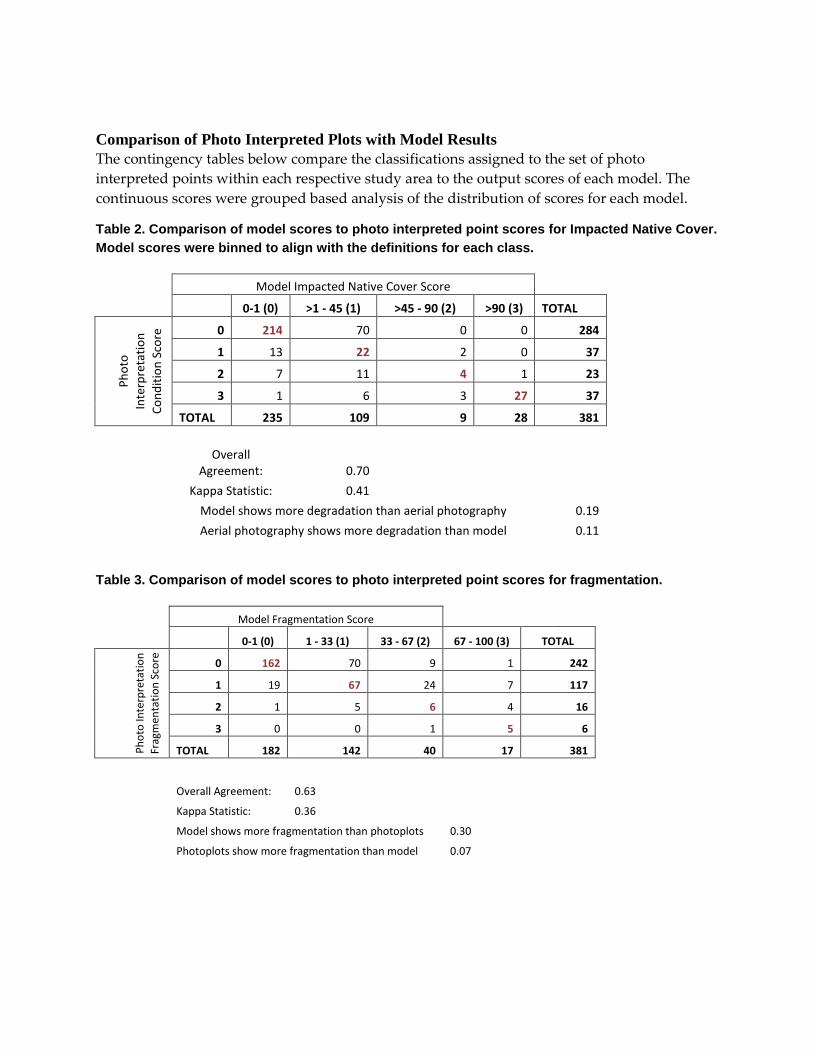
Comparison of Photo Interpreted Plots with Model Results The contingency tables below compare the classifications assigned to the set of photo interpreted points within each respective study area to the output scores of each model. The continuous scores were grouped based analysis of the distribution of scores for each model.

Table 2. Comparison of model scores to photo interpreted point scores for Impacted Native Cover. Model scores were binned to align with the definitions for each class.

Model Impacted Native Cover Score

0-1 (0) >1 - 45 (1) >45 - 90 (2) >90 (3) TOTAL

Phot

o In

terp

reta

tion

Cond

ition

Sco

re 0 214 70 0 0 284

1 13 22 2 0 37

2 7 11 4 1 23

3 1 6 3 27 37

TOTAL 235 109 9 28 381

Overall Agreement: 0.70

Kappa Statistic: 0.41

Model shows more degradation than aerial photography 0.19

Aerial photography shows more degradation than model 0.11

Table 3. Comparison of model scores to photo interpreted point scores for fragmentation.

Model Fragmentation Score

0-1 (0) 1 - 33 (1) 33 - 67 (2) 67 - 100 (3) TOTAL

Phot

o In

terp

reta

tion

Frag

men

tatio

n Sc

ore

0 162 70 9 1 242

1 19 67 24 7 117

2 1 5 6 4 16

3 0 0 1 5 6

TOTAL 182 142 40 17 381



Model shows more fragmentation than photoplots 0.30

Photoplots show more fragmentation than model 0.07

Table 4. Comparison of model scores to photo interpreted point scores for degradation.

Model Degradation Score

0-1 (0) 1 - 45 (1) 45 - 90 (2) >90 (3) TOTAL

Phot

o In

terp

reta

tion

Ove

rall

Scor

e

0 128 91 6 0 225

1 15 65 8 3 91

2 2 13 9 3 27

3 0 4 4 30 38

TOTAL 145 173 27 36 381



Model shows more degradation than photoplots 0.29

Photoplots show more degradation than model 0.10

Table 5. Comparison of Human Footprint (HF) classes to photo interpreted point scores for degradation.

HF classes

1 (0) 2,3,4 (1) 5,6,7 (2) 8,9,10 (3) TOTAL

Phot

o In

terp

reta

tion

Degr

aded

Sco

re 0 21 190 49 1 261

1 3 34 32 1 70

2 0 13 25 2 40

3 0 1 27 25 53

TOTAL 24 238 133 29 424



Model shows more degradation than photoplots: 0.65

Photoplots show more degradation than model: 0.10

Table 6. Comparison of TNC overall scores to photo interpreted point scores for degradation.

TNC scores

0 (0) 0-0.3 (1) 0.3-3 (2) >3 (3) TOTAL

Phot

o In

terp

reta

tion

Ove

rall

Scor

e

0 145 66 7 2 220

1 13 38 6 0 57

2 3 15 15 2 35

3 1 8 14 26 49

TOTAL 162 127 42 30 361





Table 7. Comparison of TNC roads to photo interpreted point scores for fragmentation.

TNC roads score

0 (0) >0-0.02 (1) >0.02-0.1 (2) >0.1 (3) TOTAL

Phot

o In

terp

reta

tion

Frag

Sco

re

0 144 37 35 2 218

1 16 21 47 19 103

2 1 0 0 4 5

3 0 0 1 5 6

TOTAL 161 58 83 30 332





Model Results in Solar Energy Zones (SEZs) Table 8. Mean scores within each SEZ designated by BLM.

Mean on-site

degradation score Mean off-site impact

score Mean compatibility

score

BLM

Sol

ar

Ener

gy Z

one

(Sol

ar P

EIS)

Imperial East 8.9 87.8 48.0

Iron Mountain 1.6 73.4 37.2

Pisgah 8.8 91.3 49.8

Riverside East 3.0 52.2 27.0

Table 9. Summary of Scores within BLM-designated SEZs.

On-Site Degradation Score Mean Min Max StdDev

BLM

Sol

ar

Ener

gy Z

one

(Sol

ar P

EIS)

Imperial East 8.9 0 100 14.3 Iron Mountain 1.6 0 28 3.7

Pisgah 8.8 0 100 11.2 Riverside East 3.0 0 100 6.0

Off-site Impact Score

Mean Min Max StdDev

BLM

Sol

ar

Ener

gy Z

one

(Sol

ar P

EIS)



Compatibility Score

Mean Min Max StdDev

BLM

Sol

ar

Ener

gy Z

one

(Sol

ar P

EIS)



List of reviewers of initial model

Name Affiliation Dick Cameron, Brian Cohen, and John Randall The Nature Conservancy Ileene Anderson Center for Biological Diversity Jerre Ann Stallcup and Wayne Spencer Conservation Biology Institute Mike Howard Dudek Susan Lee and Amy Morris Aspen Environmental Group Ryan Drobek Center For Energy Efficiency And Renewable

Technologies Todd Keeler-Wolf and Diana Hickson California Department of Fish and Game Ashley Conrad-Saydeh Bureau of Land Management

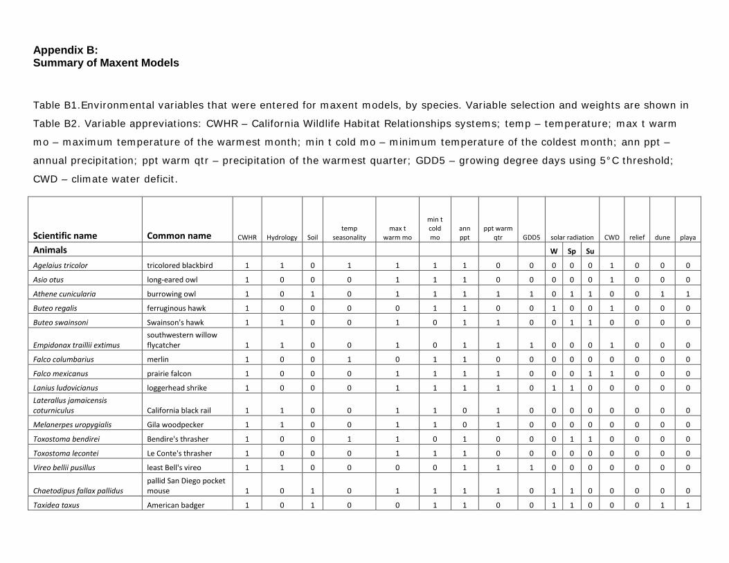
Appendix B: Summary of Maxent Models

Table B1.Environmental variables that were entered for maxent models, by species. Variable selection and weights are shown in

Table B2. Variable appreviations: CWHR – California Wildlife Habitat Relationships systems; temp – temperature; max t warm

mo – maximum temperature of the warmest month; min t cold mo – minimum temperature of the coldest month; ann ppt –

annual precipitation; ppt warm qtr – precipitation of the warmest quarter; GDD5 – growing degree days using 5°C threshold;

CWD – climate water deficit.

Scientific name Common name CWHR Hydrology Soil temp

seasonality max t

warm mo

min t cold mo

ann ppt

ppt warm qtr GDD5 solar radiation CWD relief dune playa

Animals

W Sp Su Agelaius tricolor tricolored blackbird 1 1 0 1 1 1 1 0 0 0 0 0 1 0 0 0

Asio otus long-eared owl 1 0 0 0 1 1 1 0 0 0 0 0 1 0 0 0

Athene cunicularia burrowing owl 1 0 1 0 1 1 1 1 1 0 1 1 0 0 1 1

Buteo regalis ferruginous hawk 1 0 0 0 0 1 1 0 0 1 0 0 1 0 0 0

Buteo swainsoni Swainson's hawk 1 1 0 0 1 0 1 1 0 0 1 1 0 0 0 0

Empidonax traillii extimus southwestern willow flycatcher 1 1 0 0 1 0 1 1 1 0 0 0 1 0 0 0

Falco columbarius merlin 1 0 0 1 0 1 1 0 0 0 0 0 0 0 0 0

Falco mexicanus prairie falcon 1 0 0 0 1 1 1 1 0 0 0 1 1 0 0 0

Lanius ludovicianus loggerhead shrike 1 0 0 0 1 1 1 1 0 1 1 0 0 0 0 0 Laterallus jamaicensis coturniculus California black rail 1 1 0 0 1 1 0 1 0 0 0 0 0 0 0 0

Melanerpes uropygialis Gila woodpecker 1 1 0 0 1 1 0 1 0 0 0 0 0 0 0 0

Toxostoma bendirei Bendire's thrasher 1 0 0 1 1 0 1 0 0 0 1 1 0 0 0 0

Toxostoma lecontei Le Conte's thrasher 1 0 0 0 1 1 1 0 0 0 0 0 0 0 0 0

Vireo bellii pusillus least Bell's vireo 1 1 0 0 0 0 1 1 1 0 0 0 0 0 0 0

Chaetodipus fallax pallidus pallid San Diego pocket mouse 1 0 1 0 1 1 1 1 0 1 1 0 0 0 0 0

Taxidea taxus American badger 1 0 1 0 0 1 1 0 0 1 1 0 0 0 1 1

Xerospermophilus mohavensis Mohave ground squirrel 1 0 1 1 1 0 1 1 0 0 1 0 0 1 1 1

Ovis canadensis Nelsoni Nelson's bighorn sheep 1 1 0 0 0 1 1 1 0 1 1 0 0 1 0 0

Charina trivirgata rosy boa 1 0 1 0 1 1 1 1 0 0 0 1

0 1 1

Crotalus ruber red-diamond rattlesnake 1 0 1 1 0 1 1 0 0 0 0 0 0 0 1 1

Gopherus agassizii desert tortoise 1 1 1 0 1 1 1 1 0 0 0 0 0 1 1 1

Phrynosoma blainvillii coast horned lizard 1 0 0 0 1 1 1 0 0 0 1 1 0 0 1 1

Uma scoparia Mojave fringe-toed lizard 1 0 1 0 1 1 1 1 0 0 1 1 0 0 1 1

Phrynosoma mcallii Flat-tailed horned lizard 1 1 1 0 1 1 1 1 0 0 0 1 0 1 1 1

Plants

Abronia villosa var aurita chaparral sand-verbena 0 0 1 0 0 1 1 1 1 1 1 1 1 0 1 1

Acmispon argyraeus var multicaulis scrub lotus 0 0 1 0 1 1 1 0 1 0 1 1 1 0 1 1

Allium nevadense Nevada onion 0 0 1 0 1 1 1 1 1 1 1 1 1 1 1 1

Androstephium breviflorum small-flowered androstephium 0 0 1 0 1 1 1 1 1 1 1 1 1 0 1 1

Arctomecon merriamii white bear poppy 0 0 1 0 0 1 1 1 1 1 1 1 1 0 1 1

Asclepias nyctaginifolia Mojave milkweed 0 1 1 0 1 1 1 1 1 1 1 1 1 0 1 1

Astragalus cimae var cimae Cima milk-vetch 0 0 1 0 1 1 1 1 1 1 1 1 1 0 1 1

Astragalus insularis var harwoodii Harwood's milk-vetch 0 0 1 0 1 1 1 1 1 1 1 0 1 0 1 1

Astragalus tidestromii Tidestrom's milk-vetch 0 0 1 0 1 1 1 1 1 1 1 1 1 0 1 1

Astrolepis cochisensis ssp cochisensis scaly cloak fern 0 0 1 0 1 1 1 1 1 1 1 1 1 0 1 1

Boechera shockleyi Shockley's rock-cress 0 0 1 0 1 1 1 1 1 1 1 1 1 1 1 1

Calochortus striatus alkali mariposa-lily 0 0 1 0 1 1 1 1 1 1 1 1 1 0 1 1

Castela emoryi Emory's crucifixion-thorn 0 1 1 0 1 1 1 1 1 1 1 1 1 0 1 1

Chorizanthe parryi var parryi Parry's spineflower 0 0 1 1 1 1 1 1 1 0 1 1 1 0 1 1

Cordylanthus parviflorus small-flowered bird's-beak 0 0 1 0 1 1 1 1 1 0 1 1 1 0 1 1

Coryphantha alversonii Alverson's foxtail cactus 0 1 1 0 1 1 1 1 1 1 1 1 1 0 1 1

Coryphantha chlorantha desert pincushion 0 0 1 0 1 1 1 1 1 1 1 1 1 0 1 1

Cymopterus deserticola desert cymopterus 0 0 1 0 1 1 1 1 1 1 1 1 1 0 1 1

Cymopterus gilmanii Gilman's cymopterus 0 0 1 0 1 1 1 1 1 1 1 1 1 1 1 1

Cymopterus multinervatus purple-nerve cymopterus 0 0 1 0 1 1 1 1 1 1 1 1 1 1 1 1

Delphinium recurvatum recurved larkspur 0 0 1 1 1 1 1 1 1 1 1 1 1 1 1 1

Enneapogon desvauxii nine-awned pappus grass 0 0 1 0 1 1 1 1 1 1 1 1 1 0 1 1

Eriastrum harwoodii Harwood's eriastrum 0 0 1 0 1 1 1 1 1 1 1 1 1 0 1 1

Erioneuron pilosum hairy erioneuron 0 0 1 0 1 1 1 1 1 1 1 1 1 1 1 1

Eriophyllum mohavense Barstow woolly sunflower 0 0 1 0 1 1 1 1 1 1 1 1 1 0 1 1

Eschscholzia minutiflora ssp twisselmannii Red Rock poppy 0 0 1 0 1 1 1 1 1 1 1 1 1 1 1 1

Grusonia parishii matted cholla 0 0 1 0 1 1 1 1 1 1 1 1 1 0 0 0

Layia heterotricha pale-yellow layia 0 0 1 0 1 1 1 1 1 1 1 1 1 1 1 1

Mentzelia tridentata threetooth blazingstar 0 0 1 0 1 1 1 1 1 1 1 1 1 0 0 0

Mimulus mohavensis Mojave monkeyflower 0 1 1 0 1 1 1 1 1 0 1 1 1 0 1 1

Monardella robisonii Robison's monardella 0 0 1 0 1 1 1 1 1 0 1 1 1 0 1 1

Muhlenbergia appressa appressed muhly 0 0 1 0 1 1 1 1 1 1 1 1 1 0 1 1

Opuntia basilaris var treleasei Bakersfield cactus 0 0 1 0 1 1 1 1 1 0 1 1 1 0 1 1

Pellaea truncata spiny cliff-brake 0 0 1 0 1 1 1 1 1 1 1 1 1 0 1 1

Penstemon albomarginatus white-margined beardtongue 0 0 1 0 1 1 1 1 1 1 1 1 1 0 1 1

Penstemon stephensii Stephens' beardtongue 0 1 1 0 1 1 1 1 1 1 1 1 1 0 1 1

Penstemon utahensis Utah beardtongue 0 0 1 0 1 1 1 1 1 1 1 1 1 0 1 1

Phacelia nashiana Charlotte's phacelia 0 0 1 0 1 1 1 1 1 1 1 1 1 0 1 1

Psorothamnus fremontii var attenuatus

narrow-leaved psorothamnus 0 0 1 0 1 1 1 1 1 1 1 1 1 0 1 1

Sanvitalia abertii Abert's sanvitalia 0 1 1 0 1 1 1 1 1 1 1 1 1 0 1 1

Senna covesii Cove's cassia 0 1 1 0 1 1 1 1 1 1 1 1 1 0 1 1

Sphaeralcea rusbyi var eremicola Rusby's desert-mallow 0 0 1 0 1 1 1 1 1 1 1 1 1 0 1 1

Stipa arida Mormon needle grass 0 0 1 0 1 1 1 1 1 1 1 1 1 0 1 1

Symphyotrichum defoliatum San Bernardino aster 0 0 1 0 1 1 1 1 1 1 1 1 1 0 1 1

Yucca brevifolia Joshua tree 0 0 1 0 1 1 1 1 1 1 1 1 1 0 1 1

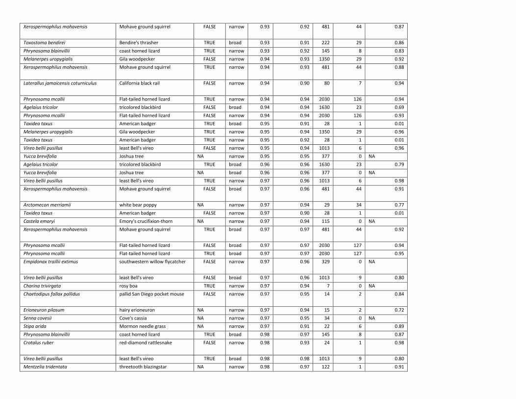
Table B2. Maxent model results. This table lists species scientific and common names, domain (narrow vs. broad), average and

best model fits based on the 10 replicate runs (AUC value), the threshold probability value used to produce the

presence/absence map, the percent contribution of each variable entered into the model, and the number of species

observations used in fitting the model.

Scientific name Common name

with CWHR

NHD hydro

CWHR maxT warm

minT cold

ppt warm

temp season

NHD peren

flow accum

ann ppt

gdd5 arid soil field capac

soil poros

soil thick

playa soil water store

dunes soil pH

spr solar

relief

Lanius ludovicianus

loggerhead shrike

FALSE NA NA 21.33 14.98 34.94 NA NA NA 14.98 NA NA NA NA NA NA NA NA NA 13.77 NA

Lanius ludovicianus

loggerhead shrike

FALSE NA NA 22.84 16.24 30.66 NA NA NA 16.96 NA NA NA NA NA NA NA NA NA 13.30 NA

Lanius ludovicianus

loggerhead shrike

TRUE NA 28.53 17.88 6.65 25.33 NA NA NA 11.01 NA NA NA NA NA NA NA NA NA 10.60 NA

Lanius ludovicianus

loggerhead shrike

TRUE NA 27.79 17.32 8.66 25.01 NA NA NA 9.91 NA NA NA NA NA NA NA NA NA 11.31 NA

Toxostoma lecontei

Le Conte's thrasher

FALSE NA NA 34.96 40.49 NA NA NA NA 24.54 NA NA NA NA NA NA NA NA NA NA NA

Toxostoma lecontei

Le Conte's thrasher

FALSE NA NA 31.40 36.41 NA NA NA NA 32.19 NA NA NA NA NA NA NA NA NA NA NA

Toxostoma lecontei

Le Conte's thrasher

TRUE NA 13.12 32.06 33.74 NA NA NA NA 21.07 NA NA NA NA NA NA NA NA NA NA NA

Falco mexicanus prairie falcon FALSE NA NA 16.01 12.95 39.11 NA NA NA 6.75 NA 9.52 NA NA NA NA NA NA NA 15.66 NA

Falco mexicanus prairie falcon FALSE NA NA 14.85 14.53 38.57 NA NA NA 9.62 NA 6.78 NA NA NA NA NA NA NA 15.65 NA

Toxostoma lecontei

Le Conte's thrasher

TRUE NA 11.67 23.80 30.69 NA NA NA NA 33.83 NA NA NA NA NA NA NA NA NA NA NA

Falco mexicanus prairie falcon TRUE NA 23.89 11.46 8.22 35.39 NA NA NA 4.30 NA 3.31 NA NA NA NA NA NA NA 13.43 NA

Falco mexicanus prairie falcon TRUE NA 25.12 10.14 9.36 35.53 NA NA NA 2.88 NA 4.07 NA NA NA NA NA NA NA 12.91 NA

Asio otus long-eared owl

FALSE NA NA 30.06 23.78 NA NA NA NA 36.03 NA 10.14 NA NA NA NA NA NA NA NA NA

Falco columbarius merlin FALSE NA NA NA 21.55 NA 62.97 NA NA 15.48 NA NA NA NA NA NA NA NA NA NA NA

Falco columbarius merlin FALSE NA NA NA 15.84 NA 69.39 NA NA 14.78 NA NA NA NA NA NA NA NA NA NA NA


FALSE NA NA 26.87 24.68 NA NA NA NA 33.40 NA 15.05 NA NA NA NA NA NA NA NA NA


TRUE NA 9.01 27.93 18.45 NA NA NA NA 31.07 NA 13.53 NA NA NA NA NA NA NA NA NA

Buteo regalis ferruginous hawk

FALSE NA NA NA 23.22 NA NA NA NA 19.56 NA 16.05 NA NA NA NA NA NA NA 41.17 NA

Buteo swainsoni Swainson's hawk

FALSE 10.66 NA 14.19 NA 49.37 NA 10.66 0.80 9.38 NA NA NA NA NA NA NA NA NA 15.60 NA

Toxostoma bendirei

Bendire's thrasher

FALSE NA NA 50.21 NA NA 9.19 NA NA 24.54 NA NA NA NA NA NA NA NA NA 16.07 NA


TRUE NA 13.72 27.33 15.98 NA NA NA NA 31.88 NA 11.09 NA NA NA NA NA NA NA NA NA

Athene cunicularia burrowing owl

FALSE NA NA 3.07 1.64 14.75 NA NA NA 0.68 9.17 NA 2.10 0.96 32.07 0.84 25.70 0.00 1.48 7.55 NA

Agelaius tricolor tricolored blackbird

FALSE 26.95 NA 21.98 18.91 NA 5.94 26.95 2.97 10.66 NA 12.59 NA NA NA NA NA NA NA NA NA


FALSE 11.54 NA 14.31 NA 49.86 NA 11.54 1.12 7.22 NA NA NA NA NA NA NA NA NA 15.94 NA


FALSE NA NA NA 24.43 NA NA NA NA 19.13 NA 18.49 NA NA NA NA NA NA NA 37.95 NA


TRUE NA 3.99 2.73 1.32 14.94 NA NA NA 1.24 6.97 NA 0.71 0.61 31.16 0.74 25.14 0.00 1.83 8.61 NA


FALSE NA NA 3.11 1.39 13.98 NA NA NA 0.60 11.20 NA 2.04 0.75 34.43 0.73 22.89 0.00 1.56 7.32 NA

Toxostoma bendirei

Bendire's thrasher

TRUE NA 31.01 35.81 NA NA 4.87 NA NA 16.82 NA NA NA NA NA NA NA NA NA 11.48 NA


TRUE NA 3.24 2.30 1.12 13.62 NA NA NA 0.45 9.37 NA 1.11 0.56 33.29 0.64 25.74 0.04 1.49 7.02 NA

Falco columbarius merlin TRUE NA 60.68 NA 9.45 NA 24.93 NA NA 4.95 NA NA NA NA NA NA NA NA NA NA NA

Toxostoma bendirei

Bendire's thrasher

FALSE NA NA 32.46 NA NA 12.66 NA NA 40.10 NA NA NA NA NA NA NA NA NA 14.79 NA


TRUE NA 68.90 NA 7.13 NA NA NA NA 1.68 NA 4.90 NA NA NA NA NA NA NA 17.39 NA

Falco columbarius merlin TRUE NA 59.10 NA 13.36 NA 22.79 NA NA 4.74 NA NA NA NA NA NA NA NA NA NA NA


TRUE NA 64.28 NA 9.11 NA NA NA NA 2.14 NA 5.03 NA NA NA NA NA NA NA 19.44 NA


TRUE 4.85 37.18 11.99 NA 30.62 NA 4.85 0.65 4.70 NA NA NA NA NA NA NA NA NA 10.01 NA


TRUE 5.80 38.60 11.01 NA 29.23 NA 5.80 0.90 4.05 NA NA NA NA NA NA NA NA NA 10.41 NA


TRUE 17.06 39.10 9.90 12.41 NA 3.71 17.06 2.37 7.66 NA 7.78 NA NA NA NA NA NA NA NA NA

Taxidea taxus American badger

FALSE NA NA NA 9.50 NA NA NA NA 18.65 NA NA 4.33 0.28 55.36 0.21 2.06 0.01 0.96 8.65 NA

Phrynosoma blainvillii

coast horned lizard

FALSE NA NA 14.38 26.97 NA NA NA NA 48.56 NA NA NA NA NA 0.00 NA 0.00 NA 10.09 NA

Xerospermophilus mohavensis

Mohave ground squirrel

FALSE NA NA 5.59 NA 12.80 8.26 NA NA 8.81 NA NA 2.26 6.06 3.60 0.18 11.26 0.02 5.93 7.34 27.88

Toxostoma bendirei

Bendire's thrasher

TRUE NA 32.91 23.25 NA NA 6.64 NA NA 25.29 NA NA NA NA NA NA NA NA NA 11.91 NA


coast horned lizard

TRUE NA 10.07 7.53 25.62 NA NA NA NA 46.92 NA NA NA NA NA 0.00 NA 0.00 NA 9.86 NA

Melanerpes uropygialis

Gila woodpecker

FALSE 22.52 NA 34.39 10.10 30.34 NA 22.52 2.65 NA NA NA NA NA NA NA NA NA NA NA NA



TRUE NA 14.79 4.99 NA 12.73 6.26 NA NA 6.26 NA NA 1.75 4.29 3.37 0.10 9.23 0.11 4.90 8.41 22.83

Laterallus jamaicensis coturniculus

California black rail


Phrynosoma mcallii

Flat-tailed horned lizard

TRUE 0.02 6.18 23.03 14.88 19.84 NA 0.02 0.18 14.79 NA NA 1.05 6.78 6.85 0.00 1.39 1.02 1.89 1.30 0.80


FALSE 15.69 NA 19.94 22.11 NA 13.05 15.69 1.33 23.13 NA 4.74 NA NA NA NA NA NA NA NA NA

Phrynosoma mcallii


FALSE 0.03 NA 23.08 14.69 25.99 NA 0.03 0.21 13.99 NA NA 1.39 6.40 7.00 0.00 1.38 0.13 3.99 0.95 0.76


TRUE NA 5.99 NA 8.09 NA NA NA NA 15.19 NA NA 4.44 0.54 51.13 0.11 2.14 0.00 1.70 10.68 NA


Gila woodpecker

TRUE 16.85 23.01 25.02 9.73 23.03 NA 16.85 2.37 NA NA NA NA NA NA NA NA NA NA NA NA


TRUE NA 1.98 NA 5.05 NA NA NA NA 15.13 NA NA 2.86 0.03 57.61 0.50 6.25 0.05 2.76 7.77 NA

Vireo bellii pusillus least Bell's FALSE 2.93 NA NA NA 6.61 NA 2.93 51.51 8.93 30.03 NA NA NA NA NA NA NA NA NA NA

vireo

Yucca brevifolia Joshua tree NA NA NA 7.58 16.73 7.91 NA NA NA 14.71 10.54 29.87 4.42 1.27 1.80 0.00 1.54 0.00 1.68 1.96 NA


TRUE 8.45 63.36 8.51 11.68 NA 2.00 8.45 0.93 3.49 NA 1.57 NA NA NA NA NA NA NA NA NA

Yucca brevifolia Joshua tree NA NA NA 4.23 19.71 7.96 NA NA NA 21.84 13.05 23.60 2.82 0.77 1.96 0.00 1.32 0.00 0.89 1.83 NA

Vireo bellii pusillus least Bell's vireo

TRUE 0.51 58.68 NA NA 2.46 NA 0.51 15.53 2.34 20.47 NA NA NA NA NA NA NA NA NA NA



FALSE NA NA 13.97 NA 33.06 8.58 NA NA 7.91 NA NA 1.44 4.91 2.12 0.04 5.23 0.03 3.96 10.17 8.58

Arctomecon merriamii

white bear poppy

NA NA NA NA 2.25 9.69 NA NA NA 2.60 5.78 6.70 3.73 6.49 0.77 0.00 58.44 0.00 0.95 2.59 NA


FALSE NA NA NA 6.59 NA NA NA NA 18.58 NA NA 4.27 0.18 57.47 0.58 3.84 0.01 1.28 7.22 NA

Castela emoryi Emory's crucifixion-thorn

NA 0.00 NA 15.20 3.23 16.71 NA 0.00 8.16 3.09 2.54 19.78 2.60 0.42 8.86 3.50 8.39 0.05 3.71 3.76 NA



TRUE NA 14.37 9.71 NA 31.72 5.66 NA NA 3.46 NA NA 0.62 3.56 2.23 0.05 6.47 0.05 3.92 10.67 7.52

Phrynosoma mcallii


FALSE 0.00 NA 17.73 40.08 17.63 NA 0.00 0.02 18.10 NA NA 0.32 3.04 0.60 0.01 0.12 0.10 2.01 0.12 0.11

Phrynosoma mcallii


TRUE 0.00 1.12 20.98 36.49 18.80 NA 0.00 0.03 16.26 NA NA 0.20 2.89 0.79 0.00 0.28 0.39 1.19 0.22 0.35

Empidonax traillii extimus

southwestern willow flycatcher

FALSE 18.56 NA 17.81 NA 3.45 NA 18.56 40.08 10.45 6.14 3.51 NA NA NA NA NA NA NA NA NA


FALSE 1.28 NA NA NA 9.41 NA 1.28 31.66 33.93 23.72 NA NA NA NA NA NA NA NA NA NA

Charina trivirgata rosy boa TRUE NA 29.54 1.04 1.04 9.91 NA NA NA 6.25 NA NA 0.85 0.22 9.68 0.00 0.20 0.00 40.19 1.08 NA

Chaetodipus fallax pallidus

pallid San Diego pocket mouse

FALSE NA NA 1.47 14.24 3.79 NA NA NA 43.71 NA NA 9.00 3.92 3.47 NA 14.33 NA 2.31 3.77 NA

Erioneuron pilosum

hairy erioneuron

NA NA NA 15.61 46.98 0.82 NA NA NA 0.86 6.43 0.77 0.81 0.80 15.13 0.00 2.53 0.00 1.92 1.18 6.17

Senna covesii Cove's cassia NA 0.00 NA 37.21 12.38 1.67 NA 0.00 1.81 0.24 3.70 4.66 0.30 1.02 11.74 0.00 2.92 0.00 21.66 0.68 NA

Stipa arida Mormon needle grass

NA NA NA 3.53 26.74 8.76 NA NA NA 2.20 27.88 4.89 0.41 9.70 1.64 0.00 5.37 0.00 7.52 1.37 NA


coast horned lizard

TRUE NA 5.37 7.89 15.30 NA NA NA NA 67.82 NA NA NA NA NA 0.00 NA 0.00 NA 3.62 NA

Crotalus ruber red-diamond rattlesnake

FALSE NA NA NA 5.92 NA 58.97 NA NA 20.93 NA NA 0.79 2.49 2.09 0.00 6.58 0.00 2.22 NA NA


TRUE 0.30 46.48 NA NA 3.60 NA 0.30 13.52 19.38 16.71 NA NA NA NA NA NA NA NA NA NA

Mentzelia tridentata

threetooth blazingstar

NA NA NA 5.81 2.14 34.17 NA NA NA 11.12 1.33 4.01 1.92 2.84 29.81 NA 5.38 NA 1.01 0.45 NA

Pellaea truncata spiny cliff-brake

NA NA NA 35.91 24.98 1.86 NA NA NA 0.12 25.75 0.30 0.17 0.84 8.14 0.00 1.56 0.00 0.31 0.08 NA


coast horned lizard

FALSE NA NA 9.42 16.78 NA NA NA NA 70.27 NA NA NA NA NA 0.00 NA 0.00 NA 3.53 NA

Calochortus striatus

alkali mariposa-lily

NA NA NA 0.45 5.47 32.40 NA NA NA 0.68 2.56 7.26 0.54 3.37 7.00 0.04 2.07 0.00 35.77 2.38 NA

Astragalus insularis var harwoodii

Harwood's milk-vetch

NA NA NA 22.16 21.70 22.98 NA NA NA 2.22 8.55 5.45 4.77 1.45 7.46 0.17 0.94 0.05 1.03 1.07 NA

Castela emoryi Emory's crucifixion-thorn

NA 0.00 NA 6.09 2.32 25.64 NA 0.00 3.11 1.22 6.31 30.80 3.32 0.23 5.27 4.68 4.75 0.14 1.90 4.24 NA

Charina trivirgata rosy boa TRUE NA 24.39 2.56 11.51 7.24 NA NA NA 2.63 NA NA 1.99 0.63 12.32 0.00 3.06 0.00 32.73 0.94 NA


narrow-leaved psorothamnus

NA NA NA 7.79 7.41 6.78 NA NA NA 3.72 0.85 16.37 3.17 4.29 15.90 0.00 27.41 0.00 1.73 4.58 NA

Charina trivirgata rosy boa FALSE NA NA 3.46 8.82 13.39 NA NA NA 12.52 NA NA 0.06 4.72 11.89 0.00 1.58 0.00 38.25 5.31 NA

Cymopterus deserticola

desert cymopterus

NA NA NA 0.95 2.58 15.55 NA NA NA 0.46 26.83 16.29 18.09 5.48 0.63 0.06 4.10 0.00 7.87 1.11 NA

Coryphantha alversonii

Alverson's foxtail cactus

NA 0.22 NA 9.78 21.73 13.19 NA 0.22 1.28 4.63 12.85 6.54 3.14 2.98 6.04 0.00 7.31 0.00 5.77 4.54 NA


Gila woodpecker



Gila woodpecker


Eriophyllum mohavense

Barstow woolly sunflower

NA NA NA 3.86 8.66 48.86 NA NA NA 7.52 6.84 7.42 7.65 0.79 2.93 0.01 2.77 0.00 0.85 1.85 NA

Calochortus striatus

alkali mariposa-lily

NA NA NA 0.88 16.84 42.18 NA NA NA 0.48 2.68 2.89 0.50 0.92 10.92 0.02 1.30 0.00 18.12 2.26 NA

Eriastrum harwoodii

Harwood's eriastrum

NA NA NA 23.35 16.99 7.31 NA NA NA 1.75 34.85 1.10 1.29 3.54 0.86 0.02 2.58 3.01 0.87 2.48 NA

Phacelia nashiana Charlotte's phacelia

NA NA NA 5.32 11.18 17.52 NA NA NA 19.62 3.81 0.73 0.75 12.03 20.59 0.00 2.21 0.00 4.86 1.39 NA

Androstephium breviflorum

small-flowered androstephium

NA NA NA 7.31 15.08 10.70 NA NA NA 17.18 12.29 2.10 2.20 2.26 3.78 0.37 4.55 0.15 12.02 10.00 NA

Astragalus tidestromii

Tidestrom's milk-vetch

NA NA NA 5.76 27.27 7.41 NA NA NA 5.59 17.80 2.08 0.13 1.42 1.63 0.00 0.44 0.00 11.23 19.23 NA

Arctomecon merriamii

white bear poppy


Coryphantha chlorantha

desert pincushion

NA NA NA 1.07 11.61 25.63 NA NA NA 0.47 0.24 0.30 34.45 2.76 0.18 0.00 20.60 0.00 0.71 1.99 NA



FALSE 31.49 NA 9.68 NA 2.91 NA 31.49 28.91 19.55 4.51 2.96 NA NA NA NA NA NA NA NA NA



TRUE 8.42 29.10 15.58 NA 2.84 NA 8.42 31.56 5.09 5.49 1.91 NA NA NA NA NA NA NA NA NA

Stipa arida Mormon needle grass

NA NA NA 0.05 26.00 13.63 NA NA NA 20.10 25.98 0.87 0.63 0.68 1.82 0.00 8.22 0.00 1.22 0.80 NA

Symphyotrichum defoliatum

San Bernardino aster

NA NA NA 0.52 7.25 9.09 NA NA NA 33.45 0.00 0.85 0.74 1.95 32.28 0.00 7.02 0.00 5.20 1.65 NA

Boechera shockleyi

Shockley's rock-cress

NA NA NA 9.73 8.03 1.33 NA NA NA 18.18 9.55 10.72 4.23 6.82 5.25 0.06 9.26 0.00 16.37 0.18 0.28




Abronia villosa var aurita

chaparral sand-verbena


Grusonia parishii matted cholla





Cymopterus gilmanii

Gilman's cymopterus

NA NA NA 6.31 2.45 14.59 NA NA NA 2.12 0.01 1.11 6.32 31.95 4.61 0.00 20.96 0.00 1.16 0.39 8.02

Sanvitalia abertii Abert's NA 0.00 NA 5.50 3.95 34.47 NA 0.00 3.90 0.92 0.19 2.34 6.43 27.22 3.56 0.00 6.05 0.00 2.81 2.66 NA

sanvitalia

Astragalus insularis var harwoodii

Harwood's milk-vetch

NA NA NA 20.84 40.67 19.37 NA NA NA 11.69 1.41 0.71 1.55 0.49 2.77 0.05 0.17 0.06 0.04 0.18 NA

Penstemon albomarginatus

white-margined beardtongue

NA NA NA 10.69 1.72 23.89 NA NA NA 11.25 14.32 7.01 5.98 0.13 1.94 0.08 6.10 0.99 7.52 8.39 NA

Uma scoparia Mojave fringe-toed lizard

FALSE NA NA 27.20 25.06 18.97 NA NA NA 11.28 NA NA 0.56 3.58 5.23 0.22 0.12 0.10 3.08 4.62 NA

Boechera shockleyi

Shockley's rock-cress

NA NA NA 4.03 18.61 4.34 NA NA NA 4.67 30.55 11.01 1.74 8.82 1.65 0.04 2.81 0.00 11.60 0.09 0.04

Androstephium breviflorum

small-flowered androstephium

NA NA NA 16.52 14.73 10.55 NA NA NA 9.00 9.29 4.16 0.88 2.09 4.08 0.42 2.48 0.00 17.81 7.97 NA

Cymopterus deserticola

desert cymopterus

NA NA NA 0.17 9.38 42.62 NA NA NA 0.15 9.39 15.47 1.39 2.08 0.76 0.01 5.82 0.00 2.24 10.50 NA

Coryphantha chlorantha

desert pincushion

NA NA NA 0.13 13.25 58.26 NA NA NA 0.13 3.69 1.23 7.66 0.12 0.01 0.00 7.87 0.00 7.40 0.24 NA

Asclepias nyctaginifolia

Mojave milkweed

NA 0.71 NA 1.00 10.85 9.21 NA 0.71 2.70 0.81 2.04 1.08 39.35 6.83 6.66 0.00 1.28 0.00 11.85 5.64 NA


TRUE NA 11.44 25.15 26.76 14.67 NA NA NA 8.70 NA NA 0.48 2.60 3.44 0.13 0.03 0.02 1.17 5.41 NA

Eriophyllum mohavense

Barstow woolly sunflower

NA NA NA 1.98 2.34 46.12 NA NA NA 5.26 10.64 16.80 4.03 0.69 0.52 0.00 0.98 0.00 0.21 10.43 NA

Mimulus mohavensis

Mojave monkeyflower

NA 0.00 NA 3.95 19.64 13.70 NA 0.00 2.97 13.80 5.12 1.28 4.79 1.94 9.95 0.00 11.27 0.00 4.65 6.93 NA

Eriastrum harwoodii

Harwood's eriastrum

NA NA NA 28.36 25.14 15.63 NA NA NA 1.66 6.32 13.83 0.56 1.91 0.63 0.00 2.36 1.00 1.85 0.77 NA

Allium nevadense Nevada onion

NA NA NA 0.95 7.49 43.78 NA NA NA 1.03 10.66 8.76 1.32 5.34 7.03 0.00 5.42 0.00 0.33 5.10 2.79

Chorizanthe parryi var parryi

Parry's spineflower

NA NA NA 19.69 7.02 11.58 5.46 NA NA 2.67 6.10 1.28 32.47 1.88 0.88 0.00 4.46 0.00 2.82 3.69 NA


FALSE NA NA 34.88 15.67 19.15 NA NA NA 20.44 NA NA 1.49 1.31 1.92 0.03 0.01 0.04 0.51 4.56 NA


TRUE NA 8.34 30.98 16.76 18.67 NA NA NA 19.20 NA NA 0.81 1.44 1.31 0.00 0.02 0.02 0.24 2.20 NA


TRUE NA 11.64 NA 15.25 NA 41.19 NA NA 5.75 NA NA 1.22 4.34 8.86 0.00 3.66 0.00 8.09 NA NA



TRUE 22.57 35.32 7.03 NA 1.53 NA 22.57 18.03 9.72 4.90 0.88 NA NA NA NA NA NA NA NA NA

Coryphantha alversonii

Alverson's foxtail cactus

NA 0.11 NA 2.85 20.05 21.34 NA 0.11 0.26 18.33 4.41 4.67 3.61 4.28 10.94 0.00 5.28 0.00 1.06 2.81 NA

Monardella robisonii

Robison's monardella

NA NA NA 0.42 1.25 27.98 NA NA NA 0.02 8.08 48.61 4.12 0.38 2.30 0.00 5.15 0.00 0.51 1.18 NA

Phacelia nashiana Charlotte's phacelia

NA NA NA 0.76 6.87 26.35 NA NA NA 21.02 2.73 0.14 2.44 13.38 17.12 0.00 1.28 0.00 7.42 0.50 NA

Penstemon utahensis

Utah beardtongue

NA NA NA 2.91 0.29 1.11 NA NA NA 1.47 0.02 48.63 1.45 3.96 26.80 0.00 3.57 0.00 4.72 5.06 NA

Sphaeralcea rusbyi var eremicola

Rusby's desert-mallow

NA NA NA 0.44 24.90 29.23 NA NA NA 0.43 1.80 0.94 17.68 5.83 1.61 0.00 15.55 0.00 0.37 1.23 NA

Mimulus mohavensis

Mojave monkeyflower

NA 0.00 NA 3.79 21.60 11.88 NA 0.00 0.92 6.10 16.58 9.20 3.95 0.21 7.45 0.00 10.60 0.00 3.40 4.32 NA

Opuntia basilaris var treleasei

Bakersfield cactus

NA NA NA 1.52 51.27 14.32 NA NA NA 4.42 2.94 12.80 3.11 0.55 1.85 0.00 1.99 0.00 4.39 0.84 NA

Cymopterus multinervatus

purple-nerve cymopterus

NA NA NA 2.54 4.01 10.27 NA NA NA 0.08 1.19 6.20 1.17 27.01 2.76 0.08 17.70 0.00 0.04 0.50 26.44

Enneapogon desvauxii

nine-awned pappus grass

NA NA NA 1.41 7.13 12.18 NA NA NA 0.04 2.35 0.33 50.28 1.12 1.25 0.00 6.66 0.00 12.92 4.33 NA

Astragalus tidestromii

Tidestrom's milk-vetch

NA NA NA 3.85 32.33 9.63 NA NA NA 0.77 16.00 0.45 0.28 0.28 0.57 0.02 0.46 0.00 30.09 5.26 NA

Senna covesii Cove's cassia NA 0.00 NA 16.83 1.16 31.23 NA 0.00 0.86 1.53 7.72 19.63 1.49 0.26 16.50 0.00 0.34 0.00 1.45 0.99 NA

Cordylanthus parviflorus

small-flowered bird's-beak

NA NA NA 7.43 64.43 3.53 NA NA NA 0.00 8.54 0.08 1.65 1.27 4.23 0.00 0.87 0.00 7.94 0.04 NA



TRUE NA 22.89 0.71 11.48 0.51 NA NA NA 40.85 NA NA 3.30 2.02 0.24 NA 10.56 NA 2.19 5.26 NA

Grusonia parishii matted cholla


Mentzelia tridentata

threetooth blazingstar


Opuntia basilaris var treleasei

Bakersfield cactus

NA NA NA 11.18 3.84 56.41 NA NA NA 5.97 0.17 15.07 0.55 0.12 3.42 0.00 0.31 0.00 2.34 0.61 NA

Abronia villosa var aurita

chaparral sand-verbena


Eschscholzia minutiflora ssp twisselmannii

Red Rock poppy

NA NA NA 3.52 0.33 22.31 NA NA NA 20.34 3.30 0.01 0.35 0.62 10.48 0.00 5.22 0.00 1.83 0.24 31.46

Muhlenbergia appressa

appressed muhly

NA NA NA 25.99 3.53 36.51 NA NA NA 1.15 1.54 0.92 1.24 3.19 14.60 0.00 3.89 0.00 6.46 0.98 NA



FALSE NA NA 0.68 15.81 3.45 NA NA NA 29.61 NA NA 19.47 5.96 1.80 NA 11.49 NA 6.79 4.95 NA

Asclepias nyctaginifolia

Mojave milkweed

NA 0.31 NA 1.42 13.39 42.63 NA 0.31 0.69 0.88 3.81 0.42 11.31 1.57 0.50 0.00 0.06 0.00 17.91 5.06 NA

Erioneuron pilosum

hairy erioneuron

NA NA NA 0.12 31.79 46.77 NA NA NA 0.23 0.82 0.00 0.21 0.03 7.19 0.00 1.97 0.00 6.27 0.80 3.78

Enneapogon desvauxii

nine-awned pappus grass

NA NA NA 1.38 9.80 47.06 NA NA NA 0.32 0.62 0.25 16.28 0.54 0.30 0.00 1.57 0.00 20.21 1.67 NA

Chorizanthe parryi var parryi

Parry's spineflower

NA NA NA 4.70 2.21 3.43 59.52 NA NA 4.41 1.16 0.63 17.24 0.38 0.66 0.00 0.71 0.00 4.12 0.84 NA

Acmispon argyraeus var multicaulis

scrub lotus NA NA NA 12.45 8.54 NA NA NA NA 30.65 0.36 0.69 0.93 24.33 2.09 0.00 6.31 0.00 13.33 0.33 NA

Astrolepis cochisensis ssp cochisensis

scaly cloak fern

NA NA NA 0.58 1.40 4.30 NA NA NA 5.91 7.60 18.39 6.73 22.46 5.80 0.00 14.29 0.00 8.23 4.32 NA


FALSE NA NA NA 10.16 NA 59.43 NA NA 8.68 NA NA 2.20 5.09 8.00 0.00 0.90 0.00 5.54 NA NA

Sphaeralcea rusbyi var eremicola

Rusby's desert-mallow

NA NA NA 0.07 14.56 52.92 NA NA NA 0.11 5.94 5.01 7.92 1.05 0.59 0.00 11.31 0.00 0.08 0.43 NA

Eschscholzia minutiflora ssp twisselmannii

Red Rock poppy

NA NA NA 0.18 0.01 28.11 NA NA NA 12.32 8.17 8.06 0.05 0.11 7.86 0.00 11.63 0.00 7.00 0.02 16.47

Monardella robisonii

Robison's monardella

NA NA NA 0.26 2.45 33.31 NA NA NA 0.68 9.20 15.59 17.53 0.84 1.78 0.00 15.69 0.00 2.59 0.09 NA



TRUE NA 26.20 0.59 6.99 5.59 NA NA NA 33.25 NA NA 6.31 1.93 2.17 NA 9.97 NA 3.34 3.65 NA

Cymopterus gilmanii

Gilman's cymopterus

NA NA NA 3.24 20.39 18.70 NA NA NA 2.49 0.83 8.59 1.94 3.53 1.52 0.00 7.43 0.00 8.82 1.42 21.10

Cymopterus multinervatus

purple-nerve cymopterus

NA NA NA 0.00 6.57 50.21 NA NA NA 0.08 6.64 0.02 0.79 0.54 2.20 0.02 8.55 0.00 0.74 0.13 23.52

Muhlenbergia appressa

appressed muhly

NA NA NA 3.69 20.94 46.99 NA NA NA 1.74 0.59 1.08 0.89 1.88 14.76 0.00 3.40 0.00 3.51 0.53 NA




Astragalus cimae var cimae

Cima milk-vetch

NA NA NA 2.32 7.37 12.96 NA NA NA 2.95 49.10 12.07 0.39 4.53 2.16 0.00 0.78 0.00 3.99 1.38 NA

Acmispon argyraeus var multicaulis

scrub lotus NA NA NA 0.26 19.82 NA NA NA NA 7.29 0.30 31.23 3.60 6.69 8.28 0.00 1.07 0.00 21.05 0.40 NA

Allium nevadense Nevada onion

NA NA NA 0.01 17.01 65.42 NA NA NA 0.29 1.00 2.33 0.65 0.79 4.14 0.00 2.21 0.00 2.39 2.20 1.56

Astrolepis cochisensis ssp cochisensis

scaly cloak fern

NA NA NA 0.00 4.55 20.11 NA NA NA 0.03 12.00 11.49 1.45 4.38 3.26 0.00 16.15 0.00 24.09 2.49 NA

Penstemon stephensii

Stephens' beardtongue

NA 0.00 NA 7.83 6.36 1.04 NA 0.00 6.81 2.73 1.89 4.79 1.34 3.14 13.02 0.00 6.47 0.00 5.38 39.20 NA

Sanvitalia abertii Abert's sanvitalia

NA 0.00 NA 0.01 12.20 74.03 NA 0.00 1.65 0.02 1.43 1.27 2.91 1.22 0.44 0.00 0.35 0.00 3.41 1.08 NA


TRUE NA 3.47 NA 7.98 NA 62.06 NA NA 6.22 NA NA 1.34 2.26 11.79 0.00 0.70 0.00 4.17 NA NA

Penstemon albomarginatus

white-margined beardtongue

NA NA NA 0.30 1.38 19.12 NA NA NA 2.38 20.39 38.22 3.72 0.06 2.84 0.01 6.44 1.17 0.83 3.14 NA

Pellaea truncata spiny cliff-brake

NA NA NA 0.00 0.16 90.08 NA NA NA 1.16 0.02 2.82 2.64 0.28 0.83 0.00 0.57 0.00 1.33 0.09 NA


narrow-leaved psorothamnus

NA NA NA 0.70 2.88 32.20 NA NA NA 0.86 32.56 13.96 0.07 0.02 7.36 0.00 8.27 0.00 0.11 1.00 NA

Symphyotrichum defoliatum

San Bernardino aster

NA NA NA 0.02 9.43 20.29 NA NA NA 35.01 0.00 16.18 2.05 0.48 14.32 0.00 1.70 0.00 0.37 0.16 NA

Charina trivirgata rosy boa FALSE NA NA 1.53 5.51 9.21 NA NA NA 33.26 NA NA 1.32 1.25 13.89 0.00 0.34 0.00 33.43 0.26 NA

Layia heterotricha pale-yellow layia

NA NA NA 0.14 1.46 8.66 NA NA NA 18.72 2.44 26.44 0.72 0.69 5.23 0.00 8.07 0.00 10.74 3.93 12.77

Astragalus cimae var cimae

Cima milk-vetch

NA NA NA 0.00 12.41 83.80 NA NA NA 0.36 0.04 0.08 0.30 0.18 0.52 0.00 0.39 0.00 1.79 0.14 NA

Cordylanthus parviflorus

small-flowered bird's-beak

NA NA NA 0.00 0.01 77.30 NA NA NA 0.00 0.00 0.28 0.22 0.51 5.41 0.00 0.69 0.00 14.78 0.81 NA

Penstemon utahensis

Utah beardtongue

NA NA NA 0.04 5.87 54.16 NA NA NA 2.70 0.90 16.02 0.80 1.26 10.11 0.00 2.05 0.00 3.12 2.96 NA

Layia heterotricha pale-yellow layia

NA NA NA 0.00 11.83 29.88 NA NA NA 7.02 5.12 21.51 0.55 0.37 1.68 0.00 2.47 0.00 8.46 2.43 8.68

Penstemon Stephens' NA 0.00 NA 0.28 18.68 38.47 NA 0.00 1.10 1.70 0.00 0.01 0.94 1.23 10.72 0.00 9.59 0.00 0.15 17.14 NA

stephensii beardtongue

Delphinium recurvatum

recurved larkspur

NA NA NA 13.28 2.98 14.56 11.27 NA NA 1.02 13.59 0.32 0.24 10.55 3.33 0.00 3.11 0.00 0.85 2.51 22.39

Delphinium recurvatum

recurved larkspur

NA NA NA 2.31 5.88 25.65 6.88 NA NA 0.06 3.27 0.09 1.03 6.23 19.23 0.00 1.13 0.00 0.74 6.86 20.65

Riparia riparia Bank swallow NA NA NA NA NA NA NA NA NA NA NA NA NA NA NA NA NA NA NA NA NA

Aquila chrysaetos Golden eagle NA NA NA NA NA NA NA NA NA NA NA NA NA NA NA NA NA NA NA NA NA

Ovis canadensis Nelsoni

Nelson's bighorn sheep

NA NA NA NA NA NA NA NA NA NA NA NA NA NA NA NA NA NA NA NA NA

Antrozous pallidus pallid bat NA NA NA NA NA NA NA NA NA NA NA NA NA NA NA NA NA NA NA NA NA

Macrotus californicus

California leaf-nosed bat


Corynorhinus townsendii

Townsend's big-eared bat


Coccyzus americanus occidentalis

western yellow-billed cuckoo


Lasionycteris noctivagans

silver-haired bat


Gopherus agassizii desert tortoise


Coleonyx switaki Barefoot (Switak's banded) gecko


Euderma maculatum

spotted bat NA NA NA NA NA NA NA NA NA NA NA NA NA NA NA NA NA NA NA NA NA

Scientific name Common name with CWHR extent best auc mean auc n=10 # obs # obs 51-80 hcast mean AUC

Lanius ludovicianus loggerhead shrike FALSE narrow 0.79 0.78 11000 262 0.73 Lanius ludovicianus loggerhead shrike FALSE broad 0.80 0.79 11000 262 0.73 Lanius ludovicianus loggerhead shrike TRUE narrow 0.81 0.80 11000 262 0.77 Lanius ludovicianus loggerhead shrike TRUE broad 0.81 0.81 11000 262 0.76 Toxostoma lecontei Le Conte's thrasher FALSE narrow 0.82 0.81 1594 43 0.77 Toxostoma lecontei Le Conte's thrasher FALSE broad 0.83 0.83 1594 43 0.77 Toxostoma lecontei Le Conte's thrasher TRUE narrow 0.84 0.83 1594 43 0.80 Falco mexicanus prairie falcon FALSE broad 0.84 0.83 2472 69 0.64 Falco mexicanus prairie falcon FALSE narrow 0.85 0.83 2472 69 0.72 Toxostoma lecontei Le Conte's thrasher TRUE broad 0.85 0.84 1594 43 0.81 Falco mexicanus prairie falcon TRUE narrow 0.86 0.85 2472 69 0.72 Falco mexicanus prairie falcon TRUE broad 0.86 0.85 2472 69 0.73 Asio otus long-eared owl FALSE broad 0.86 0.85 944 48 0.85 Falco columbarius merlin FALSE broad 0.87 0.85 1538 10 0.34 Falco columbarius merlin FALSE narrow 0.87 0.85 1538 10 0.36 Asio otus long-eared owl FALSE narrow 0.87 0.85 944 48 0.85 Asio otus long-eared owl TRUE narrow 0.88 0.86 944 48 0.88 Buteo regalis ferruginous hawk FALSE narrow 0.88 0.88 1574 18 0.70 Buteo swainsoni Swainson's hawk FALSE broad 0.89 0.88 1242 33 0.81 Toxostoma bendirei Bendire's thrasher FALSE narrow 0.89 0.86 222 27 0.79 Asio otus long-eared owl TRUE broad 0.89 0.86 944 48 0.88 Athene cunicularia burrowing owl FALSE narrow 0.90 0.89 4440 64 0.87 Agelaius tricolor tricolored blackbird FALSE narrow 0.90 0.88 1630 19 0.81 Buteo swainsoni Swainson's hawk FALSE narrow 0.90 0.89 1242 33 0.80 Buteo regalis ferruginous hawk FALSE broad 0.90 0.88 1574 18 0.69 Athene cunicularia burrowing owl TRUE narrow 0.90 0.90 4440 64 0.88 Athene cunicularia burrowing owl FALSE broad 0.90 0.90 4440 64 0.87 Toxostoma bendirei Bendire's thrasher TRUE narrow 0.90 0.88 222 27 0.84 Athene cunicularia burrowing owl TRUE broad 0.90 0.90 4440 64 0.90 Falco columbarius merlin TRUE narrow 0.91 0.91 1538 10 0.74 Toxostoma bendirei Bendire's thrasher FALSE broad 0.91 0.90 222 29 0.87 Buteo regalis ferruginous hawk TRUE narrow 0.91 0.91 1574 18 0.82 Falco columbarius merlin TRUE broad 0.92 0.91 1538 10 0.71 Buteo regalis ferruginous hawk TRUE broad 0.92 0.91 1574 18 0.81 Buteo swainsoni Swainson's hawk TRUE narrow 0.92 0.91 1242 33 0.92 Buteo swainsoni Swainson's hawk TRUE broad 0.92 0.91 1242 33 0.92 Agelaius tricolor tricolored blackbird TRUE narrow 0.92 0.91 1630 19 0.92 Taxidea taxus American badger FALSE broad 0.93 0.90 28 1 0.01 Phrynosoma blainvillii coast horned lizard FALSE narrow 0.93 0.91 145 8 0.76

Xerospermophilus mohavensis Mohave ground squirrel FALSE narrow 0.93 0.92 481 44 0.87

Toxostoma bendirei Bendire's thrasher TRUE broad 0.93 0.91 222 29 0.86 Phrynosoma blainvillii coast horned lizard TRUE narrow 0.93 0.92 145 8 0.83 Melanerpes uropygialis Gila woodpecker FALSE narrow 0.94 0.93 1350 29 0.92 Xerospermophilus mohavensis Mohave ground squirrel TRUE narrow 0.94 0.93 481 44 0.88

Laterallus jamaicensis coturniculus California black rail FALSE narrow 0.94 0.90 80 7 0.94

Phrynosoma mcallii Flat-tailed horned lizard TRUE narrow 0.94 0.94 2030 126 0.94 Agelaius tricolor tricolored blackbird FALSE broad 0.94 0.94 1630 23 0.69 Phrynosoma mcallii Flat-tailed horned lizard FALSE narrow 0.94 0.94 2030 126 0.93 Taxidea taxus American badger TRUE broad 0.95 0.91 28 1 0.01 Melanerpes uropygialis Gila woodpecker TRUE narrow 0.95 0.94 1350 29 0.96 Taxidea taxus American badger TRUE narrow 0.95 0.92 28 1 0.01 Vireo bellii pusillus least Bell's vireo FALSE narrow 0.95 0.94 1013 6 0.96 Yucca brevifolia Joshua tree NA narrow 0.95 0.95 377 0 NA Agelaius tricolor tricolored blackbird TRUE broad 0.96 0.96 1630 23 0.79 Yucca brevifolia Joshua tree NA broad 0.96 0.96 377 0 NA Vireo bellii pusillus least Bell's vireo TRUE narrow 0.97 0.96 1013 6 0.98 Xerospermophilus mohavensis Mohave ground squirrel FALSE broad 0.97 0.96 481 44 0.91

Arctomecon merriamii white bear poppy NA narrow 0.97 0.94 29 34 0.77 Taxidea taxus American badger FALSE narrow 0.97 0.90 28 1 0.01 Castela emoryi Emory's crucifixion-thorn NA narrow 0.97 0.94 115 0 NA Xerospermophilus mohavensis Mohave ground squirrel TRUE broad 0.97 0.97 481 44 0.92

Phrynosoma mcallii Flat-tailed horned lizard FALSE broad 0.97 0.97 2030 127 0.94 Phrynosoma mcallii Flat-tailed horned lizard TRUE broad 0.97 0.97 2030 127 0.95 Empidonax traillii extimus southwestern willow flycatcher FALSE narrow 0.97 0.96 329 0 NA

Vireo bellii pusillus least Bell's vireo FALSE broad 0.97 0.96 1013 9 0.80 Charina trivirgata rosy boa TRUE narrow 0.97 0.94 7 0 NA Chaetodipus fallax pallidus pallid San Diego pocket mouse FALSE narrow 0.97 0.95 14 2 0.84

Erioneuron pilosum hairy erioneuron NA narrow 0.97 0.94 15 2 0.72 Senna covesii Cove's cassia NA narrow 0.97 0.95 34 0 NA Stipa arida Mormon needle grass NA narrow 0.97 0.91 22 6 0.89 Phrynosoma blainvillii coast horned lizard TRUE broad 0.98 0.97 145 8 0.87 Crotalus ruber red-diamond rattlesnake FALSE narrow 0.98 0.93 24 1 0.98

Vireo bellii pusillus least Bell's vireo TRUE broad 0.98 0.98 1013 9 0.80 Mentzelia tridentata threetooth blazingstar NA narrow 0.98 0.97 122 1 0.91

Pellaea truncata spiny cliff-brake NA narrow 0.98 0.96 11 1 0.89 Phrynosoma blainvillii coast horned lizard FALSE broad 0.98 0.97 145 8 0.84 Calochortus striatus alkali mariposa-lily NA narrow 0.98 0.98 639 6 0.89 Astragalus insularis var harwoodii Harwood's milk-vetch NA narrow 0.98 0.97 432 0 NA

Castela emoryi Emory's crucifixion-thorn NA broad 0.98 0.97 115 0 NA Charina trivirgata rosy boa TRUE broad 0.98 0.95 7 0 NA Psorothamnus fremontii var attenuatus narrow-leaved psorothamnus NA narrow 0.98 0.97 29 0 NA

Charina trivirgata rosy boa FALSE broad 0.98 0.93 7 0 NA Cymopterus deserticola desert cymopterus NA narrow 0.98 0.98 473 0 NA Coryphantha alversonii Alverson's foxtail cactus NA narrow 0.98 0.98 222 5 0.91 Melanerpes uropygialis Gila woodpecker FALSE broad 0.98 0.98 1350 30 0.96 Melanerpes uropygialis Gila woodpecker TRUE broad 0.98 0.98 1350 30 0.98 Eriophyllum mohavense Barstow woolly sunflower NA narrow 0.98 0.97 322 1 0.83

Calochortus striatus alkali mariposa-lily NA broad 0.98 0.98 639 7 0.90 Eriastrum harwoodii Harwood's eriastrum NA narrow 0.98 0.98 255 0 NA Phacelia nashiana Charlotte's phacelia NA narrow 0.98 0.98 248 0 NA Androstephium breviflorum small-flowered androstephium NA narrow 0.98 0.98 384 0 NA

Astragalus tidestromii Tidestrom's milk-vetch NA narrow 0.98 0.98 244 1 0.97 Arctomecon merriamii white bear poppy NA broad 0.98 0.97 29 34 0.88 Coryphantha chlorantha desert pincushion NA narrow 0.98 0.98 465 0 NA Empidonax traillii extimus southwestern willow flycatcher FALSE broad 0.98 0.97 329 0 NA

Empidonax traillii extimus southwestern willow flycatcher TRUE narrow 0.98 0.97 329 0 NA

Stipa arida Mormon needle grass NA broad 0.98 0.98 22 7 0.93 Symphyotrichum defoliatum San Bernardino aster NA narrow 0.98 0.98 33 0 NA

Boechera shockleyi Shockley's rock-cress NA narrow 0.98 0.98 365 12 0.88 Laterallus jamaicensis coturniculus California black rail TRUE narrow 0.98 0.96 80 7 0.96

Abronia villosa var aurita chaparral sand-verbena NA narrow 0.98 0.94 32 2 0.74 Grusonia parishii matted cholla NA narrow 0.99 0.98 214 0 NA Laterallus jamaicensis coturniculus California black rail FALSE broad 0.99 0.98 80 7 0.95

Cymopterus gilmanii Gilman's cymopterus NA narrow 0.99 0.98 39 10 0.96 Sanvitalia abertii Abert's sanvitalia NA narrow 0.99 0.98 45 0 NA Astragalus insularis var harwoodii Harwood's milk-vetch NA broad 0.99 0.99 432 0 NA

Penstemon albomarginatus white-margined beardtongue NA narrow 0.99 0.98 73 0 NA

Uma scoparia Mojave fringe-toed lizard FALSE narrow 0.99 0.98 278 0 NA

Boechera shockleyi Shockley's rock-cress NA broad 0.99 0.99 365 12 0.95 Androstephium breviflorum small-flowered androstephium NA broad 0.99 0.99 384 0 NA

Cymopterus deserticola desert cymopterus NA broad 0.99 0.99 473 0 NA Coryphantha chlorantha desert pincushion NA broad 0.99 0.99 465 0 NA Asclepias nyctaginifolia Mojave milkweed NA narrow 0.99 0.98 160 1 1.00 Uma scoparia Mojave fringe-toed lizard TRUE narrow 0.99 0.99 278 0 NA

Eriophyllum mohavense Barstow woolly sunflower NA broad 0.99 0.99 322 1 0.96

Mimulus mohavensis Mojave monkeyflower NA narrow 0.99 0.99 265 0 NA Eriastrum harwoodii Harwood's eriastrum NA broad 0.99 0.99 255 0 NA Allium nevadense Nevada onion NA narrow 0.99 0.97 24 1 0.98 Chorizanthe parryi var parryi Parry's spineflower NA narrow 0.99 0.99 143 1 0.51

Uma scoparia Mojave fringe-toed lizard FALSE broad 0.99 0.99 278 0 NA

Uma scoparia Mojave fringe-toed lizard TRUE broad 0.99 0.99 278 0 NA

Crotalus ruber red-diamond rattlesnake TRUE narrow 0.99 0.95 24 1 0.94

Empidonax traillii extimus southwestern willow flycatcher TRUE broad 0.99 0.98 329 0 NA

Coryphantha alversonii Alverson's foxtail cactus NA broad 0.99 0.99 222 5 0.97 Monardella robisonii Robison's monardella NA narrow 0.99 0.99 94 0 NA Phacelia nashiana Charlotte's phacelia NA broad 0.99 0.99 248 0 NA Penstemon utahensis Utah beardtongue NA narrow 0.99 0.98 22 1 0.91 Sphaeralcea rusbyi var eremicola Rusby's desert-mallow NA narrow 0.99 0.99 123 2 0.98

Mimulus mohavensis Mojave monkeyflower NA broad 0.99 0.99 265 0 NA Opuntia basilaris var treleasei Bakersfield cactus NA narrow 0.99 0.99 201 0 NA

Cymopterus multinervatus purple-nerve cymopterus NA narrow 0.99 0.98 36 0 NA Enneapogon desvauxii nine-awned pappus grass NA narrow 0.99 0.99 195 4 0.87

Astragalus tidestromii Tidestrom's milk-vetch NA broad 0.99 0.99 244 1 1.00 Senna covesii Cove's cassia NA broad 0.99 0.99 34 0 NA Cordylanthus parviflorus small-flowered bird's-beak NA narrow 0.99 0.98 10 2 0.76

Chaetodipus fallax pallidus pallid San Diego pocket mouse TRUE broad 0.99 0.97 14 2 0.81

Grusonia parishii matted cholla NA broad 0.99 0.99 214 0 NA Mentzelia tridentata threetooth blazingstar NA broad 0.99 0.99 122 2 0.78 Opuntia basilaris var treleasei Bakersfield cactus NA broad 0.99 0.99 201 0 NA

Abronia villosa var aurita chaparral sand-verbena NA broad 0.99 0.97 32 2 0.84 Eschscholzia minutiflora ssp twisselmannii Red Rock poppy NA narrow 0.99 0.99 146 0 NA

Muhlenbergia appressa appressed muhly NA narrow 0.99 0.96 19 0 NA Chaetodipus fallax pallidus pallid San Diego pocket mouse FALSE broad 0.99 0.95 14 2 0.75

Asclepias nyctaginifolia Mojave milkweed NA broad 0.99 0.99 160 1 0.99 Erioneuron pilosum hairy erioneuron NA broad 0.99 0.99 15 2 0.80 Enneapogon desvauxii nine-awned pappus grass NA broad 1.00 0.99 195 4 0.97

Chorizanthe parryi var parryi Parry's spineflower NA broad 1.00 0.99 143 1 0.98

Acmispon argyraeus var multicaulis scrub lotus NA narrow 1.00 0.99 35 1 0.88

Astrolepis cochisensis ssp cochisensis scaly cloak fern NA narrow 1.00 0.99 25 0 NA

Crotalus ruber red-diamond rattlesnake FALSE broad 1.00 0.99 24 1 0.98

Sphaeralcea rusbyi var eremicola Rusby's desert-mallow NA broad 1.00 0.99 123 2 1.00

Eschscholzia minutiflora ssp twisselmannii Red Rock poppy NA broad 1.00 1.00 146 0 NA

Monardella robisonii Robison's monardella NA broad 1.00 1.00 94 0 NA Chaetodipus fallax pallidus pallid San Diego pocket mouse TRUE narrow 1.00 0.95 14 2 0.75

Cymopterus gilmanii Gilman's cymopterus NA broad 1.00 0.99 39 10 0.97 Cymopterus multinervatus purple-nerve cymopterus NA broad 1.00 1.00 36 0 NA Muhlenbergia appressa appressed muhly NA broad 1.00 0.98 19 0 NA Laterallus jamaicensis coturniculus California black rail TRUE broad 1.00 0.99 80 7 0.96

Astragalus cimae var cimae Cima milk-vetch NA narrow 1.00 0.99 21 3 0.89

Acmispon argyraeus var multicaulis scrub lotus NA broad 1.00 1.00 35 1 1.00

Allium nevadense Nevada onion NA broad 1.00 0.99 24 1 1.00 Astrolepis cochisensis ssp cochisensis scaly cloak fern NA broad 1.00 0.99 25 0 NA

Penstemon stephensii Stephens' beardtongue NA narrow 1.00 0.98 15 6 0.88 Sanvitalia abertii Abert's sanvitalia NA broad 1.00 1.00 45 0 NA Crotalus ruber red-diamond rattlesnake TRUE broad 1.00 0.99 24 1 0.95

Penstemon albomarginatus white-margined beardtongue NA broad 1.00 1.00 73 0 NA

Pellaea truncata spiny cliff-brake NA broad 1.00 1.00 11 1 1.00 Psorothamnus fremontii var attenuatus narrow-leaved psorothamnus NA broad 1.00 1.00 29 0 NA

Symphyotrichum defoliatum San Bernardino aster NA broad 1.00 1.00 33 0 NA

Charina trivirgata rosy boa FALSE narrow 1.00 0.94 7 0 NA Layia heterotricha pale-yellow layia NA narrow 1.00 1.00 30 0 NA Astragalus cimae var cimae Cima milk-vetch NA broad 1.00 1.00 21 3 1.00

Cordylanthus parviflorus small-flowered bird's-beak NA broad 1.00 1.00 10 2 0.94

Penstemon utahensis Utah beardtongue NA broad 1.00 1.00 22 1 1.00 Layia heterotricha pale-yellow layia NA broad 1.00 1.00 30 0 NA Penstemon stephensii Stephens' beardtongue NA broad 1.00 0.99 15 6 0.96 Delphinium recurvatum recurved larkspur NA narrow 1.00 1.00 5 0 NA Delphinium recurvatum recurved larkspur NA broad 1.00 1.00 5 0 NA Riparia riparia Bank swallow NA NA NA NA NA NA NA Aquila chrysaetos Golden eagle NA NA NA NA NA NA NA Ovis canadensis Nelsoni Nelson's bighorn sheep NA NA NA NA NA NA NA Antrozous pallidus pallid bat NA NA NA NA NA NA NA Macrotus californicus California leaf-nosed bat NA NA NA NA NA NA NA

Corynorhinus townsendii Townsend's big-eared bat NA NA NA NA NA NA NA

Coccyzus americanus occidentalis western yellow-billed cuckoo NA NA NA NA NA NA NA

Lasionycteris noctivagans silver-haired bat NA NA NA NA NA NA NA Gopherus agassizii desert tortoise NA NA NA NA NA NA NA Coleonyx switaki Barefoot (Switak's banded) gecko NA NA NA NA NA NA NA

Euderma maculatum spotted bat NA NA NA NA NA NA NA

Appendix C: Mojavset users manual Introduction Mojavset is a spatial decision-support tool that reports the potential impacts to biodiversity from any given solar development site in the California portion of the Mojave Desert and identifies potential biodiversity offset sites for conservation action. Mojavset is an R function that runs the ZONATION (Moilanen 2012) software to prioritize sites to be considered for offsets. Mojavset generates the required Zonation input files via a series of user responses to text prompts. Along with the standard zonation output, Mojavset generates ascii grids that delineate potential offset sites and corresponding site reports with information on land management and biodiversity representation specific to the offset sites. The goal of biodiversity offsets is to achieve a net positive outcome for biodiversity when detrimental impacts to biodiversity from development cannot be avoided. Offsetting is the fourth step in the mitigation hierarchy: avoid, minimize, restore, offset. Mojavset provides decision support for the first (avoid) and the fourth (offset) steps of the mitigation hierarchy.

Avoid: Mojavset uses overlays of spatial data to provide site reports that describe potential impacts to biodiversity from development at a site. The program warns the user of potential conflicts if a development site occurs in an area that is already identified as an important area for conservation. This information allows the user to avoid the selection of development sites with the greatest impact to biodiversity and/or the greatest potential conflict with conservation objectives. Through comparison of site reports at several potential sites, the user can select development sites that will likely have less relative impact and/or conflict. Minimize: Once a site is chosen for development, the user should try to minimize the footprint at the development site. For large scale projects (i.e. projects with plans to minimize impacts that would result in changes to the development footprint that are greater than 8 hectares), the user can upload detailed shapefiles of the potential site footprint into Mojavset to compare the changes in potential impacts from alternative development plans. This is only useful in the Mojaveset program for large scale changes due to the coarse resolution of the input data (270m). Restore: The third step in the mitigation hierarchy, restore, is not considered in Mojavset due to the slow rate of recovery for delicate desert systems. Offset: The main function of Mojaveset is the prioritization of offset sites. Mojavset provides maps of potential offset sites and corresponding site reports.

1

Data Input All of the necessary input files are either created for you or are pre-packaged with the Mojavset program. However, you will have the option to upload some of your own files rather than using the provided files. If you choose to upload your own spatial data, the data must have the following properties:

Projection:

Projected Coordinate System: Albers Projection: Albers false_easting: 0.00000000 false_northing: 0.00000000 central_meridian: -96.00000000 standard_parallel_1: 29.50000000 standard_parallel_2: 45.50000000 latitude_of_origin: 23.00000000 Linear Unit: Meter Geographic Coordinate System: GCS_North_American_1983 Datum: D_North_American_1983 Prime Meridian: Greenwich Angular Unit: Degree

For Raster/ASCII data: Grid Extent:

Left: -2076990 Top: 1833000 Right: -1646610 Bottom: 1242240

Cell size: 270

2

Using the Tool

Running the Program

1. Make sure you have the R software on your computer. It is freely available for download at http://cran.us.r-project.org/

2. Download the zipped Mojavset Program. Unzip the folder. This folder contains data, code, and the Zonation program required to run Mojavset.

3. Open the Mojavset R code in a text editor (file “solar_offsets.R”) 4. Open R and copy and paste the entire “solar_offsets.R” script into the R console. It may take

several minutes to load the code. 5. To run the offsets analysis you are required to enter three functions into the R console once the

code has been loaded: createSpatialCache(), fun.input(), offsetsAnalysis(). Enter each command individually and navigate to the appropriate path or user input when prompted.

6. You can exit out of the program by hitting ESC. 7. You can restart the program once the data is loaded by typing ‘fun.input()’ into the R console.

Similarly, once the function createSpatialCache() has run, that R object can be saved and loaded at a later date.

Organization The program and manual are organized into two sections:

1. Impact analysis 2. Offset analysis

The general flow of Mojavset is:

Figure 1. Decision-support model flow. The broad structure of the decision-support tool including the general decisions available to the user and the output created from the tool.

A more detailed figure of the flow of the model with all decision branches is available in Appendix 1. User Manual The manual text describes program options and suitable user input. Boxes highlight the prompts you will receive when running the Mojavset program.

Choose Solar Development

Site

- Choose to offset impacted features vs. impacted area - Choose offset ratio - Choose offset region - Choose cost

Site report generated

Offset map created Offset site report generated

Generate Zonation input files Run Zonation

Offset Analysis Impact Analysis

3

http://cran.us.r-project.org/

IMPACT ANALYSIS

SOLAR SITE INFO Run Name

Enter a name for the run. This name will be associated with all output files. Do not use quotes or spaces.

Solar Development Site You have the option to upload your own potential solar development site as a shapefile or to use a provided map to choose a development site for the analysis.

Response must be either Y or N. The letters must be capitalized and quotes should not be used. If you enter Y, you will be prompted to enter the name of the shapefile. If you enter N, you will be prompted to choose one or more 100 hectare sites from a provided map. The 100 hectare sites are sites in which at least 90% of the area is suitable for solar development. Areas on slopes less than 5% and that have at least a value of 7 dni are considered suitable for solar development. Upload Shapefile

Enter the pathway and name of the shapefile (including suffix ‘.shp’) for the solar development site you wish to analyze. Do not use quotes. For example: C:/Users/cschloss/Documents/MOJAVE/Spatial/solar/example/example_solar_albers.shp Important: Make sure that your shapefile is a polygon shapefile and is in the Albers projection with the parameters specified in the input section of this manual (page XX). Also make sure to name the field in the attribute table that corresponds to the unique identifier for given sites as ‘Id’. Please do this even if you only have one polygon in the shapefile. Include the file type ‘.shp’ after the file name. A map will be generated for you in the plot region of the R console with the solar development sites and the boundary of the California portion of the Mojave desert.

Please input a name for the run

Are you uploading your own site?

Enter the name of the shapefile with the site - including the file pathway

4

Enter the Id of the site from the Id field in the shapefile. If the site includes many polygons with different unique identifiers you may enter multiple Id numbers separated by a comma. Do not use quotes.

If you do not choose to upload your own shapefile, you may use the provided map to identify sites you wish to analyze. You may either use the provided map and grid or use known coordinates to zoom into the region with the sites you would like to analyze. Choosing a Solar Site

Choose 1 or 2. Use map to find site (1)

Choose the approximate region for the solar development site. Type N, E, S, or W. Do not use quotes. A new map will be generated that is zoomed into the selected region. The new map will contain large-numbered grid cells. These are used only for the purpose to further zoom into the proper area of the map.

Type the ID or multiple IDs. Use a comma to separate multiple IDs. Do not use quotes. This will generate a map of the solar sites within the selected grid(s).

What is the site number? (Or enter multiple sites separated by a comma)

Do you want to use a map to find the site (1) or choose the extent surrounding your site using coordinates in the Albers_Conic_Equal_Area Projection (2)

Is the site in the North, East South, or West? Choose N, E, S or W

What is the grid ID of the region that contains the site you wish to develop for solar power? (Or enter multiple IDs separated by a comma). See provided map

5

Use bounding coordinates to find site (2)

Enter the bounding coordinates of your site. Coordinates must be in the Albers_Conic_Equal_Area projection. Four prompts (like the one above) will guide you through the longitude (westesternmost, easteasternmost) and latitude (northernmost, southousthermost) entries.

After zooming into the general region either through use of the map/grid or bounding coordinates, select the 100ha site (or multiple sites) you wish to analyze.

Choose one (or multiple) 100ha grids. These grids will be considered the solar development footprint. Each 100ha grid on this map has at least 90ha with the potential for solar development (i.e. slope <5% and receives at least 7 dni).

What is the longitude of the westernmost boundary of your site?

What is the ID of the site you wish to develop for solar power? (Or enter multiple IDs separated by a comma). See provided map

6

Site Report

Mojavset generates a report for the chosen solar site. Information in the report falls into four broad categories: land management, protection, impacted biodiversity, and solar development potential (Table 1). Table 1. The site report for any given solar development site.

Site 62203

Site Area (hectares) 116.64

Ownership (max FED area) BLM

Percent Federal Land 15.28

GAP status – area majority 3

GAP status – minimum status 3

% Priority Overlap – TNC 100

% Priority Overlap – ACEC 0

# of targeted species 8

% of targeted species 11.76

max % of range of targeted spp. 0.0104

# of ecological systems 3

% of ecological systems 17.65

max % of range of ecolog. sys. .01

Mean slope % .29

Mean DNI 7.18

Min distance to road (meters) 270

Species data in the impact analysis were modeled for 65 species using the Maximum Entropy software. Models used in the impact analysis use a broad extent (see Appendix 2) in which errors of commission were more likely than errors of omission.

7

Avoiding Impacts The first step in the mitigation hierarchy is to avoid potential harm to biodiversity. With the site report (above) you should determine whether or not to proceed with the offset analysis or if the impacts are too high and if another site would be more suitable to evaluate for development. If the potential solar development site intersects with areas identified as important for conservation, a message will appear warning you about this potential conflict with conservation priorities. The areas considered important for conservation are either a) already protected (i.e. GAP status 1 or 2), b) included in the Nature Conservancy’s (TNC) portfolio of sites, or c) included in the Bureau of Land Management’s Areas of Critical Environmental Concern (ACEC). Choose N to exit the program. Choose Y to continue to the offset analysis. We strongly recommend choosing N to exit the program if this warning appears because development in this site will likely lead to conflict with conservation objectives.

This solar development site has a X % overlap with areas identified as important for conservation and Y % of land in GAP status Z do you still want to continue? Y or N

8

OFFSET ANALYSIS

CHOOSE OFFSETS Offset Type There are 2 general methods for selecting offset sites.

1. Offset site prioritization can be specific to the features that are directly impacted by solar development at a site.

2. Offset site prioritization can be based on maximum potential for conservation gain regardless of site-specific impacts.

Offsetting impacted features – Direct Offset (option 1 above) Only features (e.g. species or ecological systems) that will be impacted by potential solar sites are used for offset prioritization. For example, if 8 species and 3 ecological systems will be impacted, then only these 11 features will be considered when prioritizing sites for offsets. The distributions of all other conservation features will be ignored and will not add value to a network of sites for offsets. Target quantities will be set for impacted features as a chosen ratio of the quantity of impacted occurrences. You will have the option to run Zonation using target-based planning which prohibits the violation of targets unless there is no other option or using a generalized-benefit function which allows, but discourages, the violation of targets, and instead, values underrepresented targets. Offsets with maximum conservation gains (option 2 above) Any conservation feature (e.g. species or ecological systems) will be available for offset prioritization. You will have the option to use all of the features or to select the specific features to be used in Zonation for offset prioritization. You will be asked to weight each feature. A weighting of 0 will remove the feature from the analysis. Higher weightings give the species more value for each occurrence. Zonation will be run two times. First, offset sites will be prioritized around the core areas of each feature (core area zonation). Second, offset sites will be prioritized based on feature richness (additive benefit function). Mojavset will produce a combined output layer highlighting the offset sites that are identified in both planning methods and the areas that are unique to each method. See the section on cell removal rules (page 36), the Zonation Manual, and the section on Mojavset Output (page 34) for more information.

Do you want to directly offset the impacted areas (1) or choose areas with maximum conservation gains (2) ?

9

Conservation Features The user can choose from several types of conservation features to prioritize areas for offsets. A table will be displayed in the R console with the types of conservation features that are available for planning (Table 2). Feature options include:

1. Species. There are 65 species included in the analysis. Modeled species were chosen based on their importance to the regional planning process. Species distributions were modeled with the Maximum Entropy (MaxEnt) software and converted to binary format based on species-specific thresholds (see appendix 2).

2. Future Species distributions – This option is not currently available in the Mojavset program. 3. Ecological systems. NatureServe Ecological Systems.

Feature types may be selected individually or used in combination with each other. Table 2. Feature types and corresponding feature codes.

Target code Biodiversity 1 Future distributions of biodiversity 2 Ecological systems 3 Biodiversity + future biodiversity 12 Biodiversity + ecological systems 13 Bio + fut bio+ ecol. sys 123

Type in the code that corresponds to the feature target or combination of features you wish to use to prioritize offset sites. Do not use quotes. Species data in the offset analysis were modeled for 65 species using the Maximum Entropy software. Models used in the offset analysis use a narrow extent (see Appendix 2) in which errors of omission were more likely than errors of commission.

Select code for targets used in prioritization

10

Feature Weights for maximum conservation priority If you have chosen to identify offsets with maximum conservation gains rather than site-specific impacts, you will be prompted to select weights for the conservation features. An editable table will be displayed in the R console.

This table contains the feature name (target), the number of occurrences of each feature impacted at the solar development site (site), the number of occurrences in the entire region (total), the code for the conservation feature (type), and the weight for the conservation feature. The default weight is an equal value for every feature (weight = 1). You may change the weights of the features by typing the selected weight in the weight column. A weight of 0 removes that specific feature from offset prioritization. A feature with a weight of 0 will not add value to offset sites or be used in Zonation for cell removal. The features with 0 a weighting will be used only for reporting purposes. Increasing weights will give species relatively more value. This will impact the order of cell-removal. Type an integer in the weight field to change the weight for a feature. Closing the editable box will automatically save your user-defined weightings.

Select weight for targets

11

Offset Ratios The offset ratio refers to units of offset per unit of impact. Units of impact can refer to the actual impacted area of the development site or to the quantity of impacted feature occurrences within the development site. The offset ratios will be applied differently depending on your choice to offset directly-impacted features or based on maximum conservation gains. Therefore, the options for offset ratios and the corresponding user prompts will be specific to your choice of offset type.

1. Directly Impacted Offset Ratios – offset ratios are used to set target quantities for each feature to be used in prioritization.

2. Offset ratios for maximum conservation gains – offset ratios are used after prioritization to identify which ranked gridcells will be considered offset sites.

Directly Impacted Offset Ratios For Direct Offsets, offset ratios will be used to set target quantities for prioritization for the impacted features. Targets will be the product of the offset ratio and the quantity of impacted occurrences. You will have the option to choose a uniform offset ratio that will be applied to all conservation features or to select a unique offset ratio for each feature or feature type.

Uniform Offset Ratio (1)

If you choose to select a uniform ratio for all conservation features you will receive a prompt to select the ratio. The format is 1 unit of impacted feature to X units of offset for that feature. Type the offset ratio of your choice. Do not use quotes. Only enter ‘X’ in a ratio in the form 1:X.

Unique offset ratios for each feature (2)

An editable table will be displayed in the R console.

Will the offset ratio be uniform (1) or unique for every target (2)?

Select offset ratio. 1:X

Choose offset ratio for each target

12

This table contains the feature name (target), the number of occurrences of each feature impacted at the solar development site (site), the number of occurrences in the entire region (total), the code for the conservation feature (type), and the offset ratio to be applied to the conservation feature. The default ratio is 1. You may change the offset ratios for any of the features by typing the selected offset ratio in the form of 1:X (type only X) in the offset column.

Offset Ratios for Maximum Conservation Gains

If you choose to prioritize offsets based on maximum conservation gains, the offset ratio will be used after prioritization to identify which of the ranked cells will be included as offsets. There are two options:

1. Impacted area. The offset will be the highest ranked cells from Zonation prioritization with a cumulative area that is the product of the impacted area (i.e. the area of the solar development site) and the offset ratio.

2. Impacted occurrences. The offset will be the highest ranked cells from Zonation prioirization with feature representation equal to targeted quantities for impacted features. Targets will be the product of the offset ratio and the quantity of impacted occurrences. Targets will not be used for prioritization and will only be used to identify which ranked cells will be identified as offset sites. Cells, therefore, could be included in the offset sites even if they do not contain occurrences of impacted targets. You will have the option to choose a uniform offset ratio that will be applied to all conservation features or to select a unique offset ratio for each feature or feature type.

Impacted Area (1) If you choose select offset sites after the Zonation prioritization ranking of cells based on a ratio of the impacted area, you will be prompted to select the ratio for the area offset.

Do you want the area of the offset sites to be based on the total impacted area (1) or based on representation of impacted features (2)?

Select area offset ratio. 1:X

13

Type the offset ratio of your choice. The format is 1 unit of impacted area to X units of offset area. Do not use quotes.

Impacted Occurrences (2)

If you choose to select offset sites after the Zonation prioritization ranking of cells based on impacted occurrences you will be prompted select an offset ratio that will be used in combination with impacted occurrences to set target values for each impacted feature. Targets will be the product of the offset ratio and the quantity of impacted occurrences. You will have the option to choose a uniform offset ratio that will be applied to all conservation features or to select a unique offset ratio for each feature or feature type.

Uniform Offset Ratio (1) If you choose to select a uniform ratio for all conservation features you will receive a prompt to select the ratio. The format is 1 unit of impacted feature to X units of offset for that feature. Type the offset ratio of your choice. Do not use quotes.

Unique offset ratios for each feature (2)

An editable table will be displayed in the R console.

This table contains the feature name (target), the number of occurrences of each feature impacted at the solar development site (site), the number of occurrences in the entire region (total), the code for the conservation feature (type), and the offset ratio to be applied to the conservation feature. The default ratio is 1. You may change the offset ratios for any of the features by typing the selected offset ratio in the form of 1:X (type only X) in the offset column.

Select offset ratio. 1:X

Choose offset ratio for each target

14

Underrepresented Targets for Direct Offsets

If you choose to prioritize offsets based on directly impacted features, you will have two options for prioritization. The main difference is 1) whether or not value is given to underrepresented features (i.e. features with representation values below their target) and 2) whether or not targets will be violated if other options for cell removal still exist. If underrepresented targets do not add value to the network, then targets will not be violated if other options exist. If underrepresented targets still add value to the network, it is possible to violate targets while other options exist.

Choosing Y will implement the generalized benefit function in Zonation as the cell removal rule. If this option is implemented targets may be violated even if other cells could be removed that do not violate targets. However, underrepresented targets will add value to the network and will be considered during prioritization. Figure 2. The generalized benefit function curve.

Should underrepresented targets still have value? Y or N?

Underrepresented Overrepresented

15

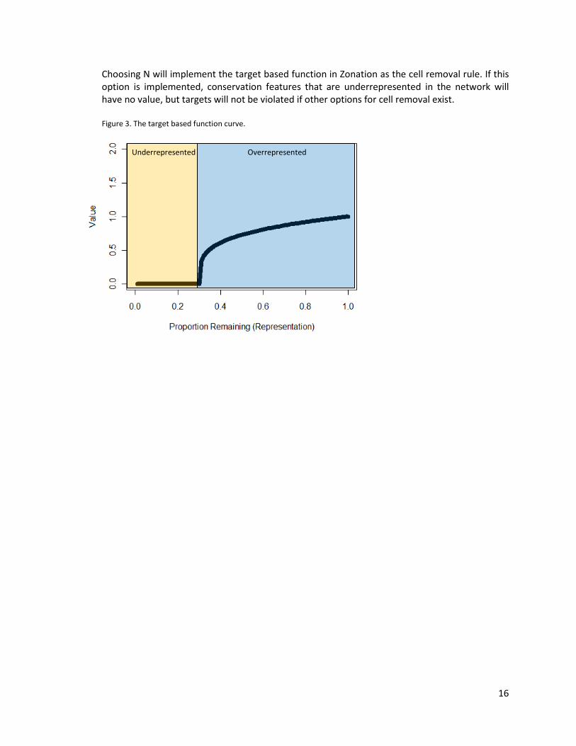
Choosing N will implement the target based function in Zonation as the cell removal rule. If this option is implemented, conservation features that are underrepresented in the network will have no value, but targets will not be violated if other options for cell removal exist. Figure 3. The target based function curve.


16

ZONATAION SETUP Mojavset creates the Zonation features file, settings file, and groups file (when used). The groups file will be created if you have chosen to plan for offsets based on two feature types (e.g. species and ecological systems). Values in all of the files are either permanently set by Mojavset or set based on your responses to text prompts. Feature File Every row in the feature file corresponds with a conservation feature. The values of the fields in each row depend on the type of prioritization you have chosen. Planning for maximum conservation gains

• Weight – the first column in the feature file is the weighting for each feature. If you have chosen to prioritize offsets based on maximum conservation gains rather than directly impacted features you were given the option to adjust the weightings of any of the biodiversity features. The default value for every feature is an equal weighting (i.e. a value of 1 for every species).

• Exponent - the fifth column is the exponent of the curve that the additive benefit function in

Zonation uses to convert changes in feature representation to changes in network value. We set this value as 0.25 because this is the default setting used for overrepresented features in the target benefit function.

Planning for directly impacted targets

• If you chose for underrepresented targets to have no value in the network • Target proportion - the fifth column in the feature file represents the targeted proportion of

feature occurrences. This is the cutoff value between under- and over-representation for the feature. This will be set for you based on the product of the offset ratio that you chose and the quantity of impacted occurrences at the solar development site.

• If you choose for underrepresented targets to have value in the network • The first and fifth columns are species weightings. The first column gives weight to the

species when it is underrepresented, the fifth column gives a weight to the species when it is overrepresented. These values are preset in Mojavset at 1.

• The sixth column represents the targeted proportion of species occurrences. This is the cutoff between under- and over-representation. This will be set for you based on the product of the offset ratio and the quantity of impacted occurrences.

• The seventh and eighth columns represent exponents for the curves that Zonation uses to convert changes in representation to changes in network value for under- and overrepresented features respectively. These are set as 1 and 0.25 respectively

Previously set: the Species file also contains information for distribution smoothing and boundary quality penalty options. Using these features of Zonation is not implemented in the Mojavset tool so these will always be set as dummy variables.

17

Groups File The groups file will only be generated and used if you have chosen to plan using more than one type of biodiversity feature (i.e. planning for both species and ecological systems). The only column in the groups file that Mojavset uses is first column which specifies the output group for each feature (row). Output statistics in Zonation will be grouped separately for each unique value in this column.

18

Settings file The settings file is the input file that contains all of the run settings for Zonation. In tableX (below) the options in green were set for you based in previous responses to text prompts, the options in blue will be adjusted based on your responses to upcoming text prompts, and the options in black are preset for you. Option Value Status

Removal rule 3 User Defined – set as 1 (CAZ) or 2 (ABF) for highest conservation priority planning and set as 3 (TBF) or 4 (GBF) for target based planning

Warp factor 1 User Defined – for highest conservation priority planning only

Edge removal 0 Preset – Not Used

Add edge points 0 Preset – Not Used

Use SSI 0 Preset – Not Used

SSI file name Preset - blank

Use planning unit layer 0 User Defined

Planning unit layer file User Defined

Use cost 0 User Defined

Cost file User Defined

Use mask 0 User Defined – Option for prioritization in zones

Mask file User-defined values create a mask for maximum conservation gains. Areas excluded from the offset analysis will receive a zone value of 1, included in the offset analysis a value of 2, and areas already protected (GAP 1 or 2) a value of 3.

Use boundary quality penalty 0 Preset – Not Used

BQP profiles file Preset - blank

BQP mode 0 Preset

BLP 0 User Defined

Use tree connectivity 0 Preset – Not Used

Tree connectivity file Preset - blank

Use interactions 0 Preset – Not Used

Interaction file Preset – blank

Annotate name 1 Preset

Logit space 0 Preset – Not Used

Zero-areas as missing data 0 Preset – Not Used

z 0.25 Preset- zonation default – species area curve esponent for extinction risk

19

Resample species 0 Preset – Not Used

Post-processing list file Preset – blank

Memory save mode 0 Preset – blank

Use groups 1 Set only if more than one type of conservation feature are chosen for offsets (i.e. species and ecological systems)

Groups file File Set only if more than one type of conservation feature are chosen for offsets (i.e. species and ecological systems)

Use condition layer 0 Preset – Not Used

Condition file Preset - blank

Use retention layer 0 Preset – Not Used

Retention file Preset - blank

Retention layers relative weight

1 Preset - default

Mask missing areas User Defined – Option for limiting offset options to certain areas

Area mask file File User Defined values create a mask. Development site and protected areas with GAP status 1&2 are automatically removed

Info-gap proportional 0 Preset – Not Used

Use info-gap weights 0 Preset – Not Used

Info-gap weights file Preset - blank

Load similarity matrix Preset - blank

Connectivity similarity matrix file

Preset - blank

Apply to connectivity 0 Preset

Connectivity edge effect fix file

0 Preset – Not Used

Community similarity matrix file

Preset - blank

Apply to representation 0 Preset – Not Used

Use ADMUs 0 Preset – Not Used

ADMU mode 1 Preset - default

ADMU layer file Preset - blank

ADMU descriptions file Preset - blank

ADMU weight matrix P Preset - blank

Mode 2 global weight 0.5 Preset - default

Row count for per ADMU output curves

0 Preset - default

20

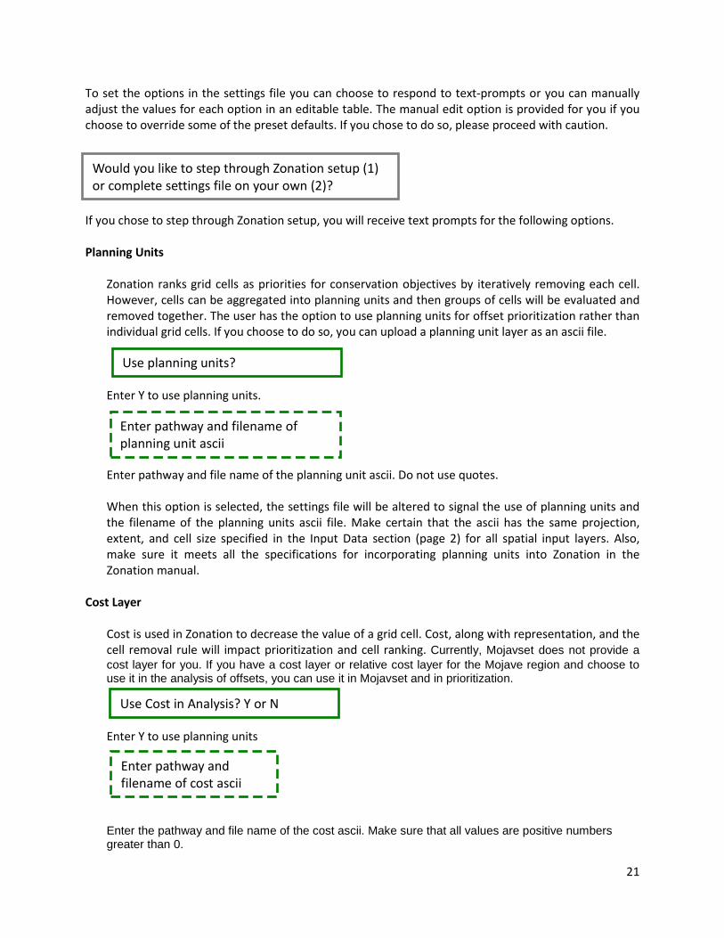
To set the options in the settings file you can choose to respond to text-prompts or you can manually adjust the values for each option in an editable table. The manual edit option is provided for you if you choose to override some of the preset defaults. If you chose to do so, please proceed with caution. If you chose to step through Zonation setup, you will receive text prompts for the following options. Planning Units

Zonation ranks grid cells as priorities for conservation objectives by iteratively removing each cell. However, cells can be aggregated into planning units and then groups of cells will be evaluated and removed together. The user has the option to use planning units for offset prioritization rather than individual grid cells. If you choose to do so, you can upload a planning unit layer as an ascii file. Enter Y to use planning units. Enter pathway and file name of the planning unit ascii. Do not use quotes. When this option is selected, the settings file will be altered to signal the use of planning units and the filename of the planning units ascii file. Make certain that the ascii has the same projection, extent, and cell size specified in the Input Data section (page 2) for all spatial input layers. Also, make sure it meets all the specifications for incorporating planning units into Zonation in the Zonation manual.

Cost Layer

Cost is used in Zonation to decrease the value of a grid cell. Cost, along with representation, and the cell removal rule will impact prioritization and cell ranking. Currently, Mojavset does not provide a cost layer for you. If you have a cost layer or relative cost layer for the Mojave region and choose to use it in the analysis of offsets, you can use it in Mojavset and in prioritization.

Enter Y to use planning units

Enter the pathway and file name of the cost ascii. Make sure that all values are positive numbers greater than 0.

Use planning units?

Enter pathway and filename of planning unit ascii

Use Cost in Analysis? Y or N

Enter pathway and filename of cost ascii

Would you like to step through Zonation setup (1) or complete settings file on your own (2)?

21

Aggregate Solutions

Cell rankings that are solely based on cell value and offset sites corresponding to these rankings may be dispersed across the region of potential offset sites. The region can be limited if you choose to specify acceptable areas for offsets through the use of a Mask (below), however, you can also aggregate solutions through the implementation of a boundary length penalty which discourages cell removal if the removal of that cell increases the perimeter to area ratio of the network. Below is the equation used to implement a Boundary Length Penalty from the Zonation User Manual.

If you choose to aggregate the solution, you will be prompted to choose several penalty values in order to investigate the impact of different values on offset site distribution. Enter values separated by a comma between 0 and 1. Do not use quotes. Zonation will be run for each boundary length penalty value you choose. It is a good idea to investigate the effect of several BLP values, but may also be time intensive.

Warp Factors

If you choose to prioritize offsets based on maximum conservation gains and are not using a boundary length penalty, you will have the option to decrease the processing time of the Zonation analysis by removing cells in groups rather than one at a time. This is recommended only for exploratory analysis rather than for the final run. Choose Y or N. If you choose Y, you will not receive the option to select a warp factor. If you choose N you will be prompted to choose warp factors.

Enter the number of cells you wish to remove with each time step.

Aggregate solution through Boundary Length Penalty (BLP)? Y or N

It is recommended that you try several values of BLP. Values should be between 0 and 1? Enter values separated by a comma.

Is this a final run?

Select # of cells to remove at each step (enter # greater than or equal to 1)

22

Manually Adjust Settings File If you chose to not to step through Zonation setup, an editable table of the settings options will appear in the R console.

Type the changes to the value field in the editable table. Closing the table will save your edits. Use caution if you choose to change Mojavset defaults.

Manually adjust defaults in settings file

23

MASKS

Mojavset automatically excludes from the offset analysis 1) the solar development site that you selected and 2) protected areas with GAP status 1 or 2. You will have the option to further specify acceptable regions for potential offset locations and, conversely, regions on which to avoid siting offsets using a mask. You can either upload a mask that specifies sites to be included as acceptable regions for offsets or create a mask by making decisions within the Mojavset program.

Mask layers are implemented differently depending on the type of prioritization you have selected for offset siting. The main differences are:

1. For directly impacted features, a mask clips the analysis region (i.e. input and output) to the region specified by the mask. Only these specified areas are used for cell-removal and prioritization. All other areas are excluded (Figures 4 & 5).

2. For maximum conservation gains, the mask specifies zones which impact the order of cell-removal. All cells are included in cell-removal and prioritization. Only the zone for potential offsets will be used to site offsets (Figures 6 & 7).

24

Figure 4. For directly impacted features, offset analysis (cell-removal and prioritization) only occur in the region available for offsets (blue).

Figure 5. For directly impacted features, cells are only removed in areas that are available for offsets. The offset sites are the regions in which all targets are met.

In offset sites In regions available for offsets

25

Figure 6. For maximum conservation gains, cells are removed from the entire region: first from the areas excluded from the analysis (red), then from the region available for potential offset sites (blue), lastly from already protected areas (green)

Figure 7. An example benefit curve for a feature corresponding to the map in Figure 4. The red region corresponds with the feature representation in areas excluded from the analysis (red), available for potential offset sites (blue), and already protected (green). The curve shows the change in cell value that corresponds to changes in representation of that feature.

Already protected

In o

ffset

site

s

In regions available for offsets

In excluded regions

26

Regardless of the method for mask implementation, offset sites will be chosen within the region you specify for the analysis. If you chose to prioritize offsets based on directly-impacted features, the mask will be used to clip your input data, the analysis region, and the output files to the region specified by the mask. This is equivalent to the “area mask” in the Zonation software. The targeted proportions of the conservation features will be recalculated as the targeted amounts (i.e. product of the impacted quantities and the offset ratios) divided by the total amount of each feature within the specified mask.

If you choose to specify areas to exclude/include either through the program options or by uploading a mask layer, Mojavset will also automatically update your specified region by excluding the footprint of the solar development site and protected areas with GAP status 1 and 2. If you choose not to use a mask, Mojavset will still generate a mask to be used in Zonation that excludes the footprint of the solar development site and protected areas with GAP status 1 and 2 from the analysis.

If you chose to prioritize offsets based on maximum conservation gains, the mask will be used to specify zones for cell removal. Cells will be removed one zone at a time from the lowest value zone to the highest value zone. This is equivalent to the “removal mask” in the Zonation software .Areas that you choose to exclude will be designated as zone 1 and will be removed first. Areas that you choose to include for offset siting will be designated as zone 2. Protected areas with GAP status 1 or 2 will be designated as zone 3. As long as the area of the offset is smaller than or equal to the area of zone2, your offset sites will be within the limits of the areas specified.

If you choose to specify areas to exclude/include either through the program options or by uploading a mask layer, the area you specify for offsets will be converted into a removal mask with a value of 2, the excluded regions in the mask will be given a 1 along with the solar development sites, and protected areas will be designated zone 3.

27

Using Masks

Enter Y if you would like to limit the area of the analysis to a certain region. Otherwise enter N. Do not use quotes.

Enter 1 to use Mojavset options to create a layer with included/excluded areas. Enter a 2 to upload your own ascii mask file.

Creating a Mask file

Mojavset allows the user to specify acceptable regions for offsets based on land management and ownership, conservation status, land cover, distance from the development site, potential for future development. A complete list of the options is listed in table XX.

Table XX. List of regions to include or exclude from offset analysis in addition to the solar development sites and protected areas with GAP status 1 and 2.

Mask Location Exclude/Include

Solar Potential -1 TNC Portfolio 0 ACEC 0 Federal Land 0 Private Land 0 Distance from site (mi) NA All Natural Land Cover Types 0 Specific Land Cover Type 0 Projected Urban Growth – High Impact Only

0

Projected Urban Growth – Low Impact

0

Projected Urban Growth 0

Enter a value of 1 for regions that must be included for potential offset sites, a value of 0 for regions that can be an offset so long as other criteria are met, and a -1 for areas that should not be included as potential offset sites.

Legally protected land (in GAP status 1 or 2) will automatically be excluded from potential offset sites. Specify other areas to include/exclude for potential offsets sites? Y or N

Would you like to create a mask layer now (1) or upload your own mask layer (2)?

28

Options may be used in concert with each other. When more than one option is specified, acceptable regions for potential offsets must meet both criteria. For example, if the user specifies that the acceptable regions for offset sites must be on federal land and must be within 25 miles of the development site, the potential offset sites must meet both of those conditions. If the user specifies that the acceptable regions for offset sites must be with 25 miles of the offset site but cannot be on land that has the potential for solar development then the acceptable areas must not have solar development potential but still must be within 25 miles of the development site.

Special Cases

Distance to development site. The default (NA) means there is no limitation for offset sites based on distance. If you choose to limit offsets to only sites within a given distance of the offset site, enter the distance in miles.

Federal land management. If you would like to avoid siting offsets on all federal lands enter a -1. If you would like to site offsets only on federal lands enter a 1. If you would like to specify potential offsets based on specific federal land types (e.g. BLM, DOD, etc) enter a 0. You will then be prompted with another table of the federal land types. You may either avoid a land type or types (-1), or specify a land type (1).

Table X. Federal lands available for inclusion/exclusion.


BLM 0 DOD 0 BIA 0 BOR 0 FWS 0 NPS 0 FS 0

Urban growth. Projected urban growth refers to areas projected to have growth based on a business as usual urban growth model. Low impact urban growth refers to areas projected to have growth with a lower relative impact do biodiversity (i.e. growth discouraged in regions important for current and future biodiversity (Thorne 2012), High impact urban growth are areas in the business as usual scenario that do not overlap with the lower relative impact areas.

29

Specific land cover type. If you would like to site offsets (or avoid siting offsets) on a specific land cover type or types, you can enter 1 or -1 in for ‘Specific land cover types’. You will then be prompted with another table with the land cover classes within the Mojave region. You may either avoid a land type or types (-1), or specify a land type (1).

Table X. Land cover classes available for inclusion/exclusion.


Water 0 Ice 0 Developed – Open 0 Developed – Low 0 Developed – Medium 0 Developed – High 0 Rock 0 Mines 0 Transitional 0 Deciduous Forest 0 Evergreen Forest 0 Mixed Forest 0 Shrubland 0 Shrub/Scrub 0 Orchards/Vineyards 0 Grasslands/Herbaceous 0 Sedge/Herbaceous 0 Lichens 0 Moss 0 Pasture/Hay 0 Row Crops 0 Small Grains 0 Fallow 0 Urban/Recreational Grasses 0 Emergent Herbaceous Wetlands

0

Uploading a mask.

The mask must meet the cell size and extent criteria for all user defined data specified on page 2 of this manual. Use a value of 1 for all acceptable regions for offset sites. Use a no data value for all regions that should be excluded (-9999 in ascii format). Mojavset will alter your user-defined mask by prohibiting offset siting in the location of the specified solar development site and in protected areas with GAP status 1 and 2. If you are planning based on maximum conservation gains, Mojavset will convert your mask to a zone layer.

30

ALTERNATIVE LAND USE Mojavset allows you to plan not only for the conservation of biodiversity features, but also for other land uses such as for solar development or urban growth. There are two ways in which Mojavset allows you to set aside land for solar development or urban growth.

1. Use a mask to limit offset sites to regions with no potential for these alternative land uses. Cells with the potential for other land uses will not be considered for offsets despite their potential value to conservation objectives.

2. Specifically plan for these land uses by decreasing the value of cells with the potential for solar development or urban growth. The biodiversity values in these cells are still considered, but the potential for other land uses are factored into the prioritization and cell ranking.

Options 1 is described in the Create Mask section of this manual (p.24). Option 2 will only be made available to you if you have not already removed each type of land use from the analysis using a mask. With this option, a layer for the alternative land use will be added as a feature file, but will have a negative weight. Removing a cell from the network of offset sites will therefore add value to, rather than decrease value from, the network. Solar potential as an alternative land use are all areas that have at least 7dni and are on slopes less than 5%. Urban growth potential as an alternative land use is based on an urban growth model with a lower relative impact do biodiversity (i.e. growth discouraged in regions important for current and future biodiversity (Thorne 2012). If you have not already planned for both solar development potential and urban growth potential using masks or zones, you will be asked if you want to plan for alternative land uses. Type Y or N. Do not use quotes. If you choose to prioritize offsets based on maximum conservation gains, you will be asked to choose a weighting for each land use available for planning (i.e. solar development potential or urban growth potential that have not been removed with a mask or specified in a zone). A weight of 0 means that that land use will not be used for prioritization.

Do you want to plan for alternative land uses? Y or N

Set a weight for Solar Potential - must be 0 or a negative number

Set a weight for Urban Develop - must be 0 or a negative number

31

Enter 0 or any negative number. Do not use quotes If you choose to prioritize offsets based on directly impacted features, you will be asked to choose a the number of acres you wish to set aside for each land use available for planning (i.e. solar development potential or urban growth potential that have not been removed with a mask or specified in a zone). Zero acres means that that land use will not be used for prioritization. Enter 0 or any positive number. Do not use quotes

How many acres should be set aside for solar development?

How many acres should be set aside for urban development?

32

Running Zonation Mojavset will generate the input text files and batch files for the Zonation runs based on your preferences. Mojavset will also generate an ascii of a mask to be used in the Zonation run. This processing step may take several minutes. If you are planning based on directly impacted targets and the region you have specified for potential offsets does not contain sufficient features to achieve the feature target quantities, then you will receive a warning message: Mojavset will then prompt you to decide whether or not to start the zonation run. Enter Y or N. If you choose Y, Zonation will be run one to potentially several times. For example, if you chose several different values of BLP, Zonation will be run separately for each level of BLP. If you chose to prioritize offsets based on maximum conservation gains, Zonation will be run separately for two cell removal rules: core-area zonation and additive benefit function.

If you choose, N. Mojavset will exit and Zonation will not be run. Your Zonation input files will be in the output folder

Do you want to run zonation?

The targets cannot be met within the mask you specified

33

OUTPUT All of the standard Zonation output is created for you. Along with:

1. Zonation input files (feature file, settings file, groups file) 2. A decision file that saves out all of the decisions you have made in Mojavset set up. 3. An ascii mask file mapping areas to include/exclude in the analysis or designating zones for

priorization. 4. A mask text file that saves your choices for inclusions/exclusions for offset locations. 5. An ascii file mapping the offset sites (Offset.Site.asc) 6. An ascii file which combines the maps the offset sites from different runs

(Offset.Site.COMBO.asc). This is only created if Zonation is run several times in one Mojavset run. For example, this file will be created if you have chosen several values of BLP or if both core area zonation and the additive benefit are run.

7. A text file key for the COMBO file describing which value corresponds with which run’s offset sites.

8. An offset site report text file. The output files will be saved in the Output Folder. All of the output files will be named with the run name that you chose and the type of Zonation cell-removal rule that was used in the zonation run (e.g. CAZ, ABF, TBF, or GBF). If BLP is used, the value of the BLP multiplied by 100 will be added to the name. If cost is used the letter C will be added. For example:

• ‘test_run.TBF’ would be a run called “test_run” that uses the target based function for prioritization.

• ‘test_run.CAZ_BLP100’ would be a run called “test_run” that uses core-area zonation and a boundary length penalty of .1

Offset Sites The ascii will be named with the name of your run and “_Offset.Site.asc”. This ascii is created from the ‘.RANK.asc’ zonation output file. The top ranked cells are chosen as offset sites. The cells that are included as offsets are either a) the top ranked cells that are necessary so that no target is violated or b) the top ranked cells that combine to a specified area. Method A is used if you have chosen to plan based on directly impacted features. It is also used if you have chosen to prioritize cells based on maximum conservation gains but to select the specific sites from the ranked cells based on impacted targets. Method B is used if you have chosen to prioritize cells based on maximum conservation gains and chose to offset the area of the impact rather than the impacted species. The area of the offset will be the product of the area of the impact and the offset area ratio. Offset Sites Combo The offset sites are combined by multiplying each offset map (1= offset site) by a factor of 10. All offset solutions are then added together. For example, a cell with a value of 1 may only be included in a core-area zonation solution, a cell with a value of 10 may only be included in an additive benefit function solution, and cell with a value of 11 is included in both solutions.

34

CELL REMOVAL RULES Zonation prioritizes grid cells for conservation by sequentially removing the cells that provide the least conservation value to the network. Cells that remain in the network the longest have the highest priority for conservation. Zonation has four rules for calculating the value of each grid cell and therefore the order of cell removal. See the Zonation manual (Moilanen 2012) for complete information on the different cell removal rules in Zonation. Here we will briefly describe them and how they are used in Mojavset.

1. Core Area Zonation 2. Additive Benefit Function 3. Target Based Function 4. Generalized Benefit Function

Core-area Zonation (CAZ) Cells are valued by the feature with the most valuable occurrence in that cell. With core-area zonation. cells with widespread features or with features that have a large proportion of their distribution remaining are considered a lower priority for conservation than cells with rare features. Only the most valuable feature is considered, and species richness is not used for prioritization. Target quantities of features are also not considered. Core-area zonation is run in Mojavset if you choose to plan based on maximum conservation gains. Additive-benefit Function (ABF) Cells are valued by the sum of the value of all features in the cell. Representation for each feature is converted to a value through a benefit function. In Mojavset, the exponent of the benefit function is set for you at 0.25. You can adjust this manually by editing the species file. Target quantities are not considered, but you can adjust the weights of different features according to your preference. The additive benefit function is run in Mojavset if you choose to plan based on maximum conservation gains.

Figure 6. The shape of the benefit-function curve for additive benefit function.

35

Target-based Function (TBF) Target quantities are set for every feature. When feature quantities in the network are greater than the target, the feature is overrepresented. When feature quantities in the network are less than the target, the feature is underrepresented. While features are overrepresented, cells receive value similarly to the additive benefit function (i.e. benefit function converts representation to value with 0.25 exponent; the cell value is the sum over all the feature values). Once a feature is underrepresented, the feature has no value. Therefore, once the first target is violated the ranked output no longer is based on all features in the analysis and should be used with caution. No target will be violated if another cell can be removed that does not violate a target. The target based function is run in Mojavset if you choose to plan based on directly impacted features, if you want to make sure targets are not violated, and if you choose for underrepresented features to have no value.

Figure 6. The shape of the benefit-function curve for target-based planning for a feature with a target of 30% of the feature’s range.


36

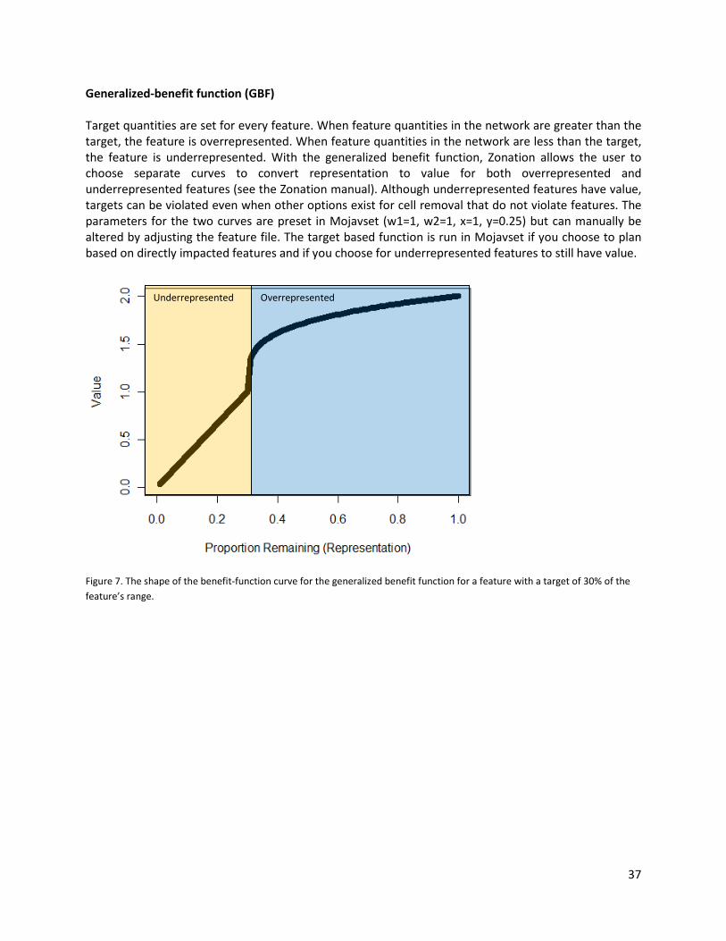
Generalized-benefit function (GBF) Target quantities are set for every feature. When feature quantities in the network are greater than the target, the feature is overrepresented. When feature quantities in the network are less than the target, the feature is underrepresented. With the generalized benefit function, Zonation allows the user to choose separate curves to convert representation to value for both overrepresented and underrepresented features (see the Zonation manual). Although underrepresented features have value, targets can be violated even when other options exist for cell removal that do not violate features. The parameters for the two curves are preset in Mojavset (w1=1, w2=1, x=1, y=0.25) but can manually be altered by adjusting the feature file. The target based function is run in Mojavset if you choose to plan based on directly impacted features and if you choose for underrepresented features to still have value.

Figure 7. The shape of the benefit-function curve for the generalized benefit function for a feature with a target of 30% of the feature’s range.


37

DATA Conservation Features

Species data Species data are modeled distributions from Maximum Entropy (MaxEnt) software (Philips et al. 2006; Phillips and Dudik 2008). A full description of the data and modeling procedure is available in Appendix 1. Each model was fitted to a broad domain which was the buffered DRECP boundary and a narrow domain which was the union of all ecological subsections where the species was observed for plants and the union of CWHRP range maps and a 10km buffer around observed ooccurances for animals. MaxEnt probability distributions were converted to binary presence/absence layers using species-specific thresholds (Appendix 2). Broad models are more likely to have errors of commission (false presence) and narrow models are more likely to have errors of omission (false absence). Mojavset uses the broad domain models to identify species that are impacted by a solar development footprint and narrow domain models to prioritize regions for offset sites. Ecological Systems Data came from Nature Serve Ecological Systems. A grid was created for each ecological system with each 270m grid cell containing the area of that ecological systems (at 30m resolution) in the 270m grid cell.

Solar Layers Solar Potential We created a map of areas with the potential for solar development as the intersection of all slopes that were less than 5% slope and were at least 7dni (Cameron et al. 2012). Potential Solar Sites We created a map of potential soalr sites by intersecting a grid with 100 ha cells (Cameron et al. 2012) with the map of solar potential. All 100 ha cells that had at least 90 ha with the potential for solar development were considered potential solar sites. Topography We created slope data (%) from 1 arc-second elevation data from the National Elevation Dataset (NED) reprojected to the Albers_conic_Equal_Area projection using bilinear resampling. U.S. Geological Survey (USGS), EROS Data Center 1999. National Elevation Dataset. U.S. Geological

Survey. Sioux Falls, SD <http://ned.usgs.gov/> Accessed: 11/9/12 DNI DNI data was obtained from the Institute of Atmospheric Physics, German Aerospace Center (DLR). Lohmann, S., C. Schillings, B. Mayer and R. Meyer (2006a): Long-term variability of solar direct and global irradiance derived from ISCCP data and comparison with re-analysis data. Solar Energy, 80, 1390-1401. http://www.pa.op.dlr.de/ISIS/isis.html. Accessed: 11/13/2012

38

http://ned.usgs.gov/

http://www.sciencedirect.com/science?_ob=ArticleURL&_udi=B6V50-4JVSSM1-4&_user=100058&_coverDate=05%2F02%2F2006&_alid=438526137&_rdoc=1&_fmt=full&_orig=search&_cdi=5772&_sort=d&_docanchor=&view=c&_acct=C000007338&_version=1&_urlVersion=0&_userid=100058&md5=5c3924e630d274ac26ed80cd32187a5a

http://www.pa.op.dlr.de/ISIS/isis.html

Land Management Federal Lands ESRI. 2010. National Atlas of the United States and the United States Geological Survey. Accessed

11/13/2012. Private Lands Department of Forestry and Fire Protection. Statewide GIS layer (GRID format) of working landscape

(areas managed for ag/timber/forage), urban and residential areas, public and private ownership, and reserves (v1). http://frap.fire.ca.gov/data/frapgisdata/download.asp?spatialdist=1&rec=mgmtscape Accessed March 11, 2013.

TNC Portfolio Sites The Nature Conservancy. 2011. Ecoregional Conservation Portfolio. http://maps.tnc.org/gis_data.html.

Accessed 7/10/2012. Areas of Critical Environmental Concern (BLM) Bureau of Land Management. 2012. Area of Critical Environmental Concern.

\\BLM\DFS\NR\Loc\Data\Data_Mgmt\3_DM_Current_Files\standards\acec\geodatabase\REVISIONS\INTERIM.gdb. Accessed 8/23/2012.

GAP data US Geological Survey (USGS) Gap Analysis Program (GAP). 2011. Protected Areas Database of the United

States (PADUS). http://gapanalysis.usgs.gov/PADUS. Accessed 11/19/2012. Land Cover Fry, J., Xian, G., Jin, S., Dewitz, J., Homer, C., Yang, L., Barnes, C., Herold, N., and Wickham, J.,

2011.Completion of the 2006 National Land Cover Database for the Conterminous United States, PE&RS, Vol. 77(9):858-864. Accessed 3/4/2013.

Distance to Roads

We created the distance to roads layer using Euclidean distance to the nearest road. The Road layer was created from the union of the following individual layers. All layers were reprojected to the Albers projection. Arizona Arizona Roads (TIGER Line - 2011). AGIC GeoData Portal https://arcgis2.geo.az.gov/portal/catalog?type_1=All&field_data_steward_accro_value=All&field_data_category_value=Transportation&tid=Accessed 5/22/2013. California Roads

Subsets of census 2007 tiger line data. The subsets contain local roads, major roads, and rail roads for all of California. Each package contains a layer file for quick viewing.

http://atlas.ca.gov/download.html#/casil/transportation. Accessed 11/16/2012 Nevada Roads http://arcdata.esri.com/data/tiger2000/tiger_statelayer.cfm?sfips=32, Accessed 5/22/2013

39

http://frap.fire.ca.gov/data/frapgisdata/download.asp?spatialdist=1&rec=mgmtscape

http://maps.tnc.org/gis_data.html

http://gapanalysis.usgs.gov/PADUS

http://www.mrlc.gov/downloadfile2.php?file=September2011PERS.pdf

http://www.mrlc.gov/downloadfile2.php?file=September2011PERS.pdf

https://arcgis2.geo.az.gov/portal/arizona-roads-tiger-line-2011

https://arcgis2.geo.az.gov/portal/catalog?type_1=All&field_data_steward_accro_value=All&field_data_category_value=Transportation&tid

https://arcgis2.geo.az.gov/portal/catalog?type_1=All&field_data_steward_accro_value=All&field_data_category_value=Transportation&tid

http://atlas.ca.gov/download.html%23/casil/transportation

http://arcdata.esri.com/data/tiger2000/tiger_statelayer.cfm?sfips=32

Urban Growth Urban Growth Potential

We used the business as usual scenario from the UPlan urban growth model output (Thorne et al. 2012) to identify areas with high potential for urban development. We used the biodiversity scenario of the urban growth model output to identify areas with the potential for urban growth with lower relative impact to biodiversity. In the biodiversity UPlan scenario, urban growth was discouraged in areas that were identified as important for the persistence of 2000 plant species across California. We also identified the areas that are in the business as usual scenario but that are absent from the biodiversity scenario as areas with urban growth potential with higher impact to biodiversity.

Thorne, J.H., Bjorkman, J., and Roth N. 2012. Urban growth in California: Projecting growth in California (2000-2050) under six alternative policy scenarios and assessing impacts to future dispersal corridors, fire threats, and climate-sensitive agriculture. University of California, Davis. p 1-72.

40

LITERATURE CITED

Cameron, D.R., Cohen, B.S., Morrison, S.A. 2012. An approach to enhance the conservation-compatibility of solar energy development. PlosOne 7(6): e38437.

Moilanen, A., Meller, L., Leppanen, J., Pouzols, F.M., Arponen, A., Kujala, H. 2012. Zonation Version 3.1 User manual. Biodviersity Conservation Informatics Group. Department of Biosciences. University of Helsinki, Finland.

Moilanen A., Leppanen, J., Pouzols, F.M. 2012. Zonation v.3.1 software. Biodviersity Conservation Informatics Group. Department of Biosciences. University of Helsinki, Finland.

Phillips S.J., Anderson R.P., Schapire R.E. (2006) Maximum entropy modeling of species geographic distributions. Ecological Modelling, 190, 231-259.

Phillips S.J., Dudík M. (2008) Modeling of species distributions with Maxent: new extensions and a

comprehensive evaluation. Ecography, 31, 161-175.

Thorne, J.H., Bjorkman, J., and Roth N. 2012. Urban growth in California: Projecting growth in California (2000-2050) under six alternative policy scenarios and assessing impacts to future dispersal corridors, fire threats, and climate-sensitive agriculture. University of California, Davis. p 1-72.

41