Embed Size (px)
Citation preview

Free Boundary Models in
Vis ous Flow
Linda Jane Cummings
St. Catherine's College
Oxford
Thesis submitted for the degree Do tor of Philosophy
Trinity Term 1996

Abstra t
The time-dependent free boundary problems of Hele-Shaw ow and slow vis ous ow (Stokes ow)
are studied, using omplex variable methods.
The �rst hapter introdu es the two problems; the mathemati al models are presented, and
brief literature reviews are given. Chapter 2 is a review of known results for the Hele-Shaw
problem, and develops the onformal mapping ideas whi h are entral to the thesis. In hapter 3,
existing work for the Stokes ow problem is reviewed and extended, and new results are presented,
prin ipally for the (singularity driven) zero surfa e tension problem on a bounded ow domain.
Chapter 4 dis usses an extension of the work of the previous hapter, as applied to sintering
problems in the glass industry. Problems on unbounded uid domains are onsidered in hapter
5, for both Hele-Shaw and Stokes ow.
Chapter 6 is on erned with singularity-driven Stokes ow, in the limit of small positive surfa e
tension. Established theory of so- alled \weak solutions" is reviewed, and applied to a new
example.
In hapter 7, the existing \ ra k" theory of Hele-Shaw ow is presented, and a new, omple-
mentary \anti ra k" model is developed. Finally, in hapter 8, we summarise and suggest ideas
for further work.

A knowledgements
I would like to thank my supervisors, Dr S. D. Howison and Dr J. R. O kendon, for guidan e
and en ouragement over the past three years. I have had several helpful dis ussions with Professors
Yuri Hohlov, John King, and Andrew La ey, and Dr Peter Howell, to whom I am very grateful.
Many thanks to Bru e and Vi ki for help with proof-reading, to James and Dan for te hni al
help, and to all the other friends at O.C.I.A.M. (espe ially DH8 members, past and present) who
have made the past three years so enjoyable. I also thank my family and Giles, for their love and
support.
Finally, I gratefully a knowledge �nan ial support from the E.P.S.R.C. in the form of an open
award, and from Smith System Engineering in the form of a s holarship and travel grant.
i

Contents
1 Introdu tion 3
1.1 Survey of the thesis . . . . . . . . . . . . . . . . . . . . . . . . . . . . . . . . . . . . 3
1.2 The Hele-Shaw problem . . . . . . . . . . . . . . . . . . . . . . . . . . . . . . . . . 4
1.2.1 The basi equations . . . . . . . . . . . . . . . . . . . . . . . . . . . . . . . 4
1.3 The Stokes ow problem . . . . . . . . . . . . . . . . . . . . . . . . . . . . . . . . . 6
1.3.1 The basi equations . . . . . . . . . . . . . . . . . . . . . . . . . . . . . . . 6
1.4 Literature Reviews and Dis ussion . . . . . . . . . . . . . . . . . . . . . . . . . . . 7
1.4.1 Hele-Shaw Flow . . . . . . . . . . . . . . . . . . . . . . . . . . . . . . . . . 7
1.4.2 Stokes ow . . . . . . . . . . . . . . . . . . . . . . . . . . . . . . . . . . . . 9
2 Complex variable methods for Hele-Shaw ow 12
2.1 Preliminaries . . . . . . . . . . . . . . . . . . . . . . . . . . . . . . . . . . . . . . . 12
2.2 The Polubarinova/Galin approa h . . . . . . . . . . . . . . . . . . . . . . . . . . . 12
2.3 The S hwarz fun tion . . . . . . . . . . . . . . . . . . . . . . . . . . . . . . . . . . 14
2.4 A simple example . . . . . . . . . . . . . . . . . . . . . . . . . . . . . . . . . . . . . 16
2.5 Ri hardson's \moments" and the Cau hy transform . . . . . . . . . . . . . . . . . 17
2.6 Transformation of the dependent variable . . . . . . . . . . . . . . . . . . . . . . . 20
2.7 Univalen y and onformality . . . . . . . . . . . . . . . . . . . . . . . . . . . . . . 23
2.8 Summary . . . . . . . . . . . . . . . . . . . . . . . . . . . . . . . . . . . . . . . . . 25
3 Complex Variable methods for Stokes ow 27
3.1 Ri hardson's approa h . . . . . . . . . . . . . . . . . . . . . . . . . . . . . . . . . . 27
3.2 Redu tion to a single equation . . . . . . . . . . . . . . . . . . . . . . . . . . . . . 31
3.2.1 Another global equation . . . . . . . . . . . . . . . . . . . . . . . . . . . . . 33
3.3 Method of solution . . . . . . . . . . . . . . . . . . . . . . . . . . . . . . . . . . . . 34
3.4 A simple example . . . . . . . . . . . . . . . . . . . . . . . . . . . . . . . . . . . . . 35
3.5 Zero surfa e tension problems . . . . . . . . . . . . . . . . . . . . . . . . . . . . . . 36
3.6 The onserved quantities . . . . . . . . . . . . . . . . . . . . . . . . . . . . . . . . . 37
3.6.1 Polynomial mapping fun tions . . . . . . . . . . . . . . . . . . . . . . . . . 38
3.6.2 Comparison with the Hele-Shaw problem | `Ri hardson's Moments' and
other matters . . . . . . . . . . . . . . . . . . . . . . . . . . . . . . . . . . . 39
3.6.3 Sour e/sink systems | a warning example . . . . . . . . . . . . . . . . . . 40
3.7 The S hwarz fun tion for the ZST problem . . . . . . . . . . . . . . . . . . . . . . 42
3.8 The \moments" for the ase �(0) 6= 0 . . . . . . . . . . . . . . . . . . . . . . . . . 46
3.9 The stress fun tion . . . . . . . . . . . . . . . . . . . . . . . . . . . . . . . . . . . . 47
3.9.1 The \Baio hi transform" for Stokes ow . . . . . . . . . . . . . . . . . . . 48
3.10 Summary . . . . . . . . . . . . . . . . . . . . . . . . . . . . . . . . . . . . . . . . . 49
4 Appli ations to the glass industry 51
4.1 Introdu tion . . . . . . . . . . . . . . . . . . . . . . . . . . . . . . . . . . . . . . . . 51
4.2 The theory for a vis ous �bre . . . . . . . . . . . . . . . . . . . . . . . . . . . . . . 51
4.3 \Conserved quantities" for �bres . . . . . . . . . . . . . . . . . . . . . . . . . . . . 53
4.3.1 Example|the sintering of a bundle of �bres . . . . . . . . . . . . . . . . . . 53
ii

4.3.2 Conne tedness onsiderations . . . . . . . . . . . . . . . . . . . . . . . . . . 55
4.4 Summary . . . . . . . . . . . . . . . . . . . . . . . . . . . . . . . . . . . . . . . . . 56
5 Flow in unbounded domains 57
5.1 Introdu tion . . . . . . . . . . . . . . . . . . . . . . . . . . . . . . . . . . . . . . . . 57
5.2 Literature Review . . . . . . . . . . . . . . . . . . . . . . . . . . . . . . . . . . . . 57
5.3 The Hele-Shaw dipole problem . . . . . . . . . . . . . . . . . . . . . . . . . . . . . 60
5.4 The Stokes ow dipole problem . . . . . . . . . . . . . . . . . . . . . . . . . . . . . 70
5.4.1 Review of Jeong & Mo�att's steady solution . . . . . . . . . . . . . . . . . 70
5.4.2 The time-dependent problem . . . . . . . . . . . . . . . . . . . . . . . . . . 72
5.5 Steady Stokes ow re onsidered . . . . . . . . . . . . . . . . . . . . . . . . . . . . . 76
5.6 Summary . . . . . . . . . . . . . . . . . . . . . . . . . . . . . . . . . . . . . . . . . 82
6 Stokes ow with small surfa e tension 83
6.1 Review of \weak" solutions . . . . . . . . . . . . . . . . . . . . . . . . . . . . . . . 83
6.2 The ubi polynomial map . . . . . . . . . . . . . . . . . . . . . . . . . . . . . . . . 85
6.2.1 Complex oeÆ ients . . . . . . . . . . . . . . . . . . . . . . . . . . . . . . . 92
6.3 Summary . . . . . . . . . . . . . . . . . . . . . . . . . . . . . . . . . . . . . . . . . 96
7 Cra k and Anti- ra k solutions to the Hele-Shaw model 97
7.1 Overview of ra ks and slits . . . . . . . . . . . . . . . . . . . . . . . . . . . . . . . 97
7.2 Introdu tion to Anti ra ks . . . . . . . . . . . . . . . . . . . . . . . . . . . . . . . . 103
7.3 Exa t ZST anti ra k solutions . . . . . . . . . . . . . . . . . . . . . . . . . . . . . . 106
7.3.1 The \generi " anti ra k . . . . . . . . . . . . . . . . . . . . . . . . . . . . . 106
7.3.2 Solutions with many anti ra ks . . . . . . . . . . . . . . . . . . . . . . . . . 109
7.3.3 Howison's radial \anti ra k" solutions . . . . . . . . . . . . . . . . . . . . . 113
7.4 The S hwarz fun tion of an anti ra k . . . . . . . . . . . . . . . . . . . . . . . . . . 114
7.5 Results from formal asymptoti s . . . . . . . . . . . . . . . . . . . . . . . . . . . . 114
7.6 Paterson's analysis . . . . . . . . . . . . . . . . . . . . . . . . . . . . . . . . . . . . 116
7.6.1 The ase �� T . . . . . . . . . . . . . . . . . . . . . . . . . . . . . . . . . . 119
7.6.2 The ase 1� � � T . . . . . . . . . . . . . . . . . . . . . . . . . . . . . . . 120
7.6.3 The ase T � �� 1 . . . . . . . . . . . . . . . . . . . . . . . . . . . . . . . 121
7.6.4 Con lusions for Paterson's anti ra ks . . . . . . . . . . . . . . . . . . . . . . 121
7.7 Fra tal Hele-Shaw . . . . . . . . . . . . . . . . . . . . . . . . . . . . . . . . . . . . 123
7.8 Cra ks revisited . . . . . . . . . . . . . . . . . . . . . . . . . . . . . . . . . . . . . . 125
7.8.1 The ase �� T . . . . . . . . . . . . . . . . . . . . . . . . . . . . . . . . . . 126
7.8.2 The ases 1� � � T , 1� �� T . . . . . . . . . . . . . . . . . . . . . . . . 127
7.9 The \ urvature onje ture" . . . . . . . . . . . . . . . . . . . . . . . . . . . . . . . 127
7.10 Extremal onformal maps . . . . . . . . . . . . . . . . . . . . . . . . . . . . . . . . 132
7.11 Summary . . . . . . . . . . . . . . . . . . . . . . . . . . . . . . . . . . . . . . . . . 135
8 Dis ussion and further work 137
8.1 Comparison of Hele-Shaw and Stokes ow . . . . . . . . . . . . . . . . . . . . . . . 137
8.2 Further work . . . . . . . . . . . . . . . . . . . . . . . . . . . . . . . . . . . . . . . 139
A Stability of blobs and bubbles in Stokes ow 140
A.1 The perturbed ir ular blob . . . . . . . . . . . . . . . . . . . . . . . . . . . . . . . 140
A.2 The perturbed ir ular bubble . . . . . . . . . . . . . . . . . . . . . . . . . . . . . . 141
B Results used for the ubi polynomial map 142
C The Stokes ow velo ity �eld in terms of w(�; t) 146
iii

List of Figures
1.1 The two phase Hele-Shaw problem. . . . . . . . . . . . . . . . . . . . . . . . . . . . . . . 5
2.1 The mapping from the unit dis onto the uid domain. . . . . . . . . . . . . . . . . . . . . 13
2.2 The mapping from the right-half plane onto the uid domain. . . . . . . . . . . . . . . . . . 14
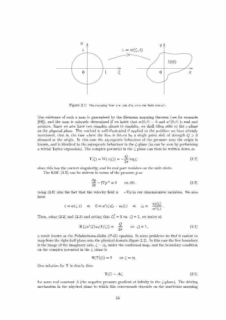
2.3 The initial and �nal domains for the quadrati polynomial mapping. . . . . . . . . . . . . . . 17
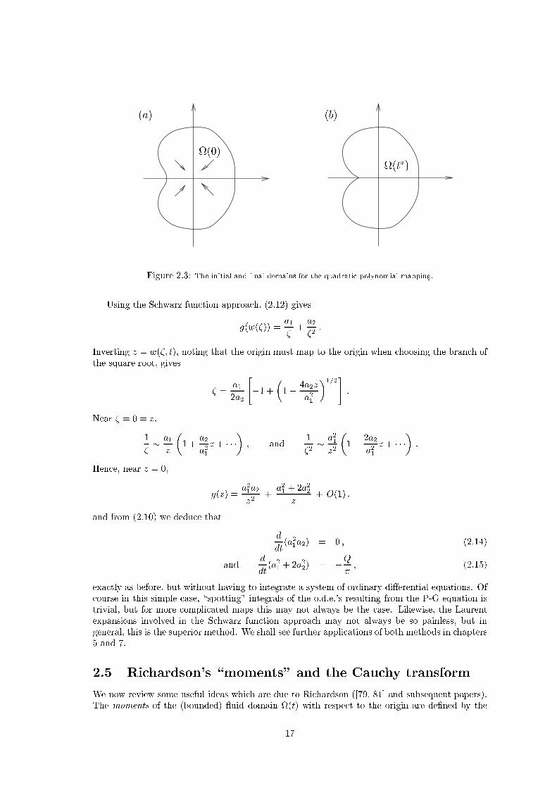
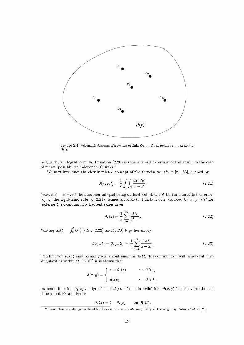
2.4 S hemati diagram of a system of sinks Q
1
; : : : Q
6
at points z
1
; : : : z
6
within (t). . . . . . . . . 19
2.5 The univalen y domain V , and phase traje tories, for the \lima� on" example of x2.4. With a
point sink, the phase paths are followed in the dire tion of the arrows (the nonunivalent region);
with a point sour e, the dire tion is opposite. Interse tion with the boundary of V is asso iated
with the usped ardioid geometry. . . . . . . . . . . . . . . . . . . . . . . . . . . . . . . 24
4.1 Typi al ross-se tions generated by the map (4.6) when n = 6. Pi ture (a) is the usped on�gu-
ration, while (b) is the kind of smooth ross-se tion we might expe t to observe in pra ti e. . . 54
5.1 S hemati diagram showing how a \ ontinuable 5/2-power usp" solution looks in phase traje tory
spa e within the univalen y domain. . . . . . . . . . . . . . . . . . . . . . . . . . . . . . 58
5.2 The geometry for the problem of a dipole pla ed o�- entre in a ir le. . . . . . . . . . . . . . 60
5.3 The geometry for the dipole-in-a-half-spa e problem. . . . . . . . . . . . . . . . . . . . . . 62
5.4 The univalen y domain in (b; )-spa e for the mapping fun tion (5.19). . . . . . . . . . . . . . 64
5.5 Typi al free boundaries generated by points (b; ) on the boundary of the univalen y domain
(�gure 5.4). The dipole is situated at the origin in ea h ase, and is su h that the x-axis is a
streamline in the positive sense. (1) has a = 1, b = 1, = 4, and has a single usp in the free
boundary; (2) has a = �1, b = 1, = �5, and has two usps in the free boundary, and (3a)
has a = �1, b = 4, = �9, and shows the free boundary beginning to overlap itself. (3b) is an
enlargement of the trapped air bubble in (3a). . . . . . . . . . . . . . . . . . . . . . . . . 65
5.6 The phase diagram (within the univalen y domain) for the Hele-Shaw dipole problem. . . . . . 67
5.7 Enlargement of the transient 5/2-power usp formation. Pi tures (a), (b) and ( ) illustrate how
the free boundary passes through the 5/2-power usped on�guration (a), to a smooth boundary
(b), before ultimately blowing up with two 3/2-power usps ( ). . . . . . . . . . . . . . . . . 68
5.8 Typi al free boundary shapes des ribed by the mapping (5.44). Case (a) has � = �0:4; � =
�5; = 0:5, and orresponds to a dipole su h that the x-axis is a streamline from negative to
positive. Case (b) has � = 1; � = 1:4; = 0:8, and has the x-axis as a streamline from positive
to negative. . . . . . . . . . . . . . . . . . . . . . . . . . . . . . . . . . . . . . . . . . 80
5.9 Typi al free boundary shape des ribed by the mapping (5.58). The parameter values used here
are � = �1; � = 3:5; = 0:65. The dipole at the origin is su h that the x-axis is a streamline
from negative to positive. . . . . . . . . . . . . . . . . . . . . . . . . . . . . . . . . . . 81
6.1 The di�erent regions in the small surfa e tension \lima� on" problem, using mat hed asymptoti s. 84
iv

6.2 Free boundary shapes des ribed by the map (6.5) for various points (b; ) on the boundary �V
of the univalen y domain. The values used are: (b
1
;
1
) = (0; 1), (b
2
;
2
) = (1; 1), (b
3
;
3
) =
(4
p
2=3; 1), (b
4
;
4
) = (1:8; 0:8461), (b
5
;
5
) = (8=5; 3=5), (b
6
;
6
) = (1; 0), and (b
7
;
7
) = (1=5;�4=5).
Pi tures (3b) and (4b) are magni� ations of the nonunivalent region, showing how the free bound-
ary begins to overlap itself; the former ase is usped and self-overlapping, while the latter is
smooth. The value a = 1 was used to generate ea h pi ture, hen e the shapes do not have equal
areas. . . . . . . . . . . . . . . . . . . . . . . . . . . . . . . . . . . . . . . . . . . . . 87
6.3 The fun tion F (b) governing evolution on the part b = 1+ of �V . (Note the di�eren e in s ales
between the two plots.) . . . . . . . . . . . . . . . . . . . . . . . . . . . . . . . . . . . 90
6.4 The univalen y diagram (restri ted to the right-half (b; )-plane) for the ubi polynomial mapping
fun tion. The shaded region orresponds to a nonunivalent map. . . . . . . . . . . . . . . . . 91
6.5 The three-dimensional univalen y domain V
z
� V
4
, and its two-dimensional ross-se tions V , V
y
and V
o
. The arrows on V
y
indi ate how the point fb = 0; = �1g destabilises ( f. �gure 6.4). . . 95
7.1 The geometry of (a) a �nite ra k; (b) a semi-in�nite ra k, along the x-axis (driven by a sink at
in�nity). . . . . . . . . . . . . . . . . . . . . . . . . . . . . . . . . . . . . . . . . . . 98
7.2 S hemati diagram showing how a general slit solution works. . . . . . . . . . . . . . . . . . 101
7.3 Examples of the radial �ngering solutions of [45℄, together with a photograph of one of Paterson's
experiments [73℄. . . . . . . . . . . . . . . . . . . . . . . . . . . . . . . . . . . . . . . . 104
7.4 Phase-�eld omputations of the \free boundary" (a tually a level set of the phase parameter �
o urring in the phase �eld model) for the growth of a seed of solid into a super ooled liquid.
This pi ture was kindly supplied by Dr A. R. Gardiner [23℄. . . . . . . . . . . . . . . . . . . 105
7.5 A typi al \generi anti ra k" solution. The free boundary is shown for times t = t
1
; t
2
; t
3
, with
t
3
> t
2
> t
1
. . . . . . . . . . . . . . . . . . . . . . . . . . . . . . . . . . . . . . . . . . 108
7.6 A typi al solution generated by (7.15), showing 4 well-developed anti ra ks. Here, ��
i
= 0:5; 1; 0:8; 0:4;
for i = 1; 2; 3; 4; respe tively; �
i
= �3; �2; 0:5; 1:5, and �
i
= 0:5 for ea h i. . . . . . . . . . . . 110
7.7 Sket h showing the geometry when we have an array of \fat anti ra ks" with narrow spa ing
generated by (7.15). The gaps between the \anti ra ks" may be viewed as ra ks. . . . . . . . 111
7.8 Solution of the form (7.15) exhibiting what we interpret as ra k and anti ra k formation. The
values �
1
= 0:1 (the anti ra k), and �
2
= �3 were used. . . . . . . . . . . . . . . . . . . . . 112
7.9 The lo al geometry with a orner of internal angle � in the uid. . . . . . . . . . . . . . . . . 115
7.10 Graph showing the relative sizes of the oeÆ ients of the terms sinn� (in the �R
1
term of R) and
os 2n� (in the �
2
R
2
term of R) as fun tions of time, in the � � T r�egime. The sinn� oÆ ient
is the upper urve. . . . . . . . . . . . . . . . . . . . . . . . . . . . . . . . . . . . . . . 120
7.11 Evolution of the free boundary of Paterson's expanding bubble for dimensionless times t =
1; 1:15; 1:3. This plot applies to the r�egime in whi h the amplitude of the perturbations is mu h
greater than T , so that the ZST perturbation theory is appli able. . . . . . . . . . . . . . . . 122
7.12 Graph showing the oÆ ients of the terms sinn� (in the �R
1
term of R) and os 2n� (in the �
2
R
2
term of R) as fun tions of time, for the �� T r�egime. The sinn� oeÆ ient is the one with initial
value 1. . . . . . . . . . . . . . . . . . . . . . . . . . . . . . . . . . . . . . . . . . . . 123
7.13 The evolving anti-slit stru ture at the stage n = 2, with 2 anti-slits of length L
0
, 2 of length L
1
,
and 4 new anti-slits about to form. . . . . . . . . . . . . . . . . . . . . . . . . . . . . . . 124
7.14 Evolution of the free boundary of the ontra ting vis ous blob in the r�egime � � T , so that the
ZST theory is appli able. The early stages of ra k formation are apparent prior to breakdown of
the linear theory. . . . . . . . . . . . . . . . . . . . . . . . . . . . . . . . . . . . . . . 128
7.15 A free boundary with ra k and anti ra k development. . . . . . . . . . . . . . . . . . . . . 129
7.16 The \Ivantsov" anti ra k solution. . . . . . . . . . . . . . . . . . . . . . . . . . . . . . . 130
7.17 Anti ra k-type stru ture generated by the map (7.57) with N = 4, � = 0:2, b(0) = 0:755,
(0) = 0:887. We see the onset of uspidal blow-up, after whi h we expe t ontinuation by ra k
or slit evolution towards the point sink. . . . . . . . . . . . . . . . . . . . . . . . . . . . 131
7.18 The ra k (a) and anti ra k (b) geometries generated by maps (7.58) and (7.59) with � = 0:1. . 132
7.19 The \open sets" interpretation of the slit geometry. . . . . . . . . . . . . . . . . . . . . . 133
7.20 The \open sets" interpretation of the anti-slit geometry. The `set of boundary points' is not open
in the topology of X. . . . . . . . . . . . . . . . . . . . . . . . . . . . . . . . . . . . . 134
1

7.21 The free boundary for a general su tion problem (with small surfa e tension). . . . . . . . . . 136
2

Chapter 1
Introdu tion
1.1 Survey of the thesis
This thesis is on erned with two di�erent free boundary problems: the Hele-Shaw problem, and
the problem of two-dimensional slow vis ous ow, or Stokes ow, as it is ommonly known. Most
of the new results we present are for the latter; however, the ( omplex variable) methods of
atta k we use for both have many similarities, and sin e histori ally the use of su h methods for
the Hele-Shaw problem predates their use for Stokes ow, we shall review the Hele-Shaw problem
�rst. The omplex variable methods used are, in any ase, probably more straightforward when
applied to Hele-Shaw ow, so this approa h has the added advantage of introdu ing the ideas to
the reader as gently as possible.
Our aim throughout the thesis is to present as uni�ed an a ount as possible; hen e wherever
pra ti able we shall keep the same notation for the two problems, this being largely that used by
Ri hardson [82℄ for the Stokes ow problem. Also in the interests of oheren e and ontinuity,
we do not stri tly segregate the two problems, but highlight similarities and ontrasts between
the two as these arise. Sin e so mu h more literature exists for the Hele-Shaw problem, su h
questions of similarities or di�eren es generally arise as we �nd a result for Stokes ow whi h has
a Hele-Shaw \analogue", or whi h is quite di�erent from the existing Hele-Shaw result.
The remainder of this hapter is devoted to introdu ing the two problems, giving a little
physi al ba kground for ea h. The governing equations and boundary onditions are derived, and
brief literature reviews are presented.
In the next two hapters solution methods for both problems are des ribed, using te hniques
from omplex variable theory. The Hele-Shaw work of hapter 2 is basi ally review; we present
it �rstly as ne essary ba kground, and se ondly be ause our results for Stokes ow provide in-
teresting analogues, and the possible link between the two problems has, ex ept for the work of
Howison & Ri hardson [49℄, been largely ignored in the literature. Chapter 3, whi h on erns
Stokes ow, ontains mainly new work. With the ex eption of xx3.1 and 3.3 (whi h review the
work of Ri hardson [82℄, but whi h present a new perspe tive on it), and x3.9 (whi h is based on
an idea due to King [58℄), the work is original (unless otherwise stated). Work whi h is losely
related to that of hapter 3, but whi h would break the ow if in luded there, is presented in
hapter 4. This on erns models of slender vis ous �bres experien ing tra tion, and is partly a
review of the work of [42℄, and partly new.
The examples onsidered in hapter 3 are all for �nite domains. Chapter 5 extends the dis us-
sion to unbounded uid domains, to reveal possible ompli ations that an arise with the Stokes
ow problem, but not in Hele-Shaw. Apart from the review material in x5.2, and x5.4.1, all the
work in this hapter is original. Both hapter 3 and hapter 5 are largely (though not ex lusively)
on erned with the zero-surfa e tension problems. The limiting ase of small, positive surfa e
tension in Stokes ow is the subje t of hapter 6, using ideas developed by Howison & Ri hardson
[49℄. After reviewing these ideas, a new example is given, and dis ussed at some length. From
x6.2 to the end of the hapter is new work.
3

The perspe tive shifts somewhat in hapter 7, whi h dis usses \ ra k" and \anti ra k" so-
lutions to the Hele-Shaw model. Se tion 7.1 reviews the established theory of ra ks, while the
remainder of the hapter is a blend of review, and original work (the distin tion is made lear in
the text). The work that is reviewed, however, is presented in a di�erent ontext in the light of
our ra k/anti ra k theory.
Finally, we dis uss our results, and suggest some possible dire tions for further work in hapter
8.
1.2 The Hele-Shaw problem
We begin by giving a short introdu tion to Hele-Shaw ow, the �rst of our free boundary problems.
A Hele-Shaw ell onsists of two rigid parallel plates some small distan e (b say) apart, between
whi h is sandwi hed one or more (immis ible) Newtonian in ompressible vis ous uids whi h an
be inje ted, su ked out, or subje ted to pressure gradients. The problem is to model the ow of
the uid within the ell. It dates ba k to Hele-Shaw's original paper [31℄, published in 1898. The
emphasis there was on the ability of the Hele-Shaw ell to reprodu e faithfully the streamlines for
invis id irrotational ow past obsta les pla ed in the ell, providing remarkable visual veri� ation
of theoreti al results. We shall be on erned with the evolution of a uid domain with a free
boundary (adja ent to a zero pressure region), under the a tion of pres ribed pressure gradients.
The problem has been extensively (though not ontinuously) studied sin e Hele-Shaw's time.
The slender geometry of the ell means that the problem is e�e tively two-dimensional, being
independent of the o-ordinate normal to the plane of the ell, whi h greatly simpli�es matters;
parti ularly fortuitous is the onsequen e that omplex variable te hniques (su h as onformal
mapping) an be applied with onsiderable su ess. We shall be using omplex variable methods
almost ex lusively throughout the thesis.
The problem is of inherent theoreti al interest, but there are various other reasons for wanting
to study it: the mathemati al model is the same as that for many important physi ally-o urring
moving boundary problems, in luding ow in porous media [75℄, �ltration [28℄, pollution of ground-
water [76℄, problems in oil and gas re overy [75℄, [41℄, ele tro hemi al ma hining [61℄, rystal
growth [72℄, inje tion moulding, and so on. In parti ular, it is a spe ial ase of the one-phase
Stefan model for phase- hange [86℄, the two models oin iding in the limit as the spe i� heat of
the medium tends to zero.
1.2.1 The basi equations
Consider �rst the more general two-phase (or \Muskat") problem of �gure 1.1, where the gap
between the plates is �lled with two uids of di�erent, onstant vis osities �
1
, �
2
, o upying
regions
1
,
2
respe tively (see for example [22℄ for a dis ussion). If b is the gap width and l the
linear dimension of the Hele-Shaw ell then under the assumption that b � l the Navier-Stokes
equations redu e
1
to
u
i
= �
b
2
12�
i
rp
i
; r:u
i
= 0 ; i = 1; 2 ;
where p
i
is the pressure in uid i and all quantities depend only on the o-ordinates in the plane
of the ell, (x; y), and time, t. Hen e the pressure is a velo ity potential for the ow, and
r
2
p
i
= 0 in
i
(t) ; i = 1; 2 :
There are two onditions holding on the free boundary � between the two uids. Firstly we have
the dynami boundary ondition (DBC), whi h omes from a for e balan e at the free boundary,
and is usually taken to be
p
2
� p
1
= �T� : (1.1)
1
See for example [71℄ for the details.
4

�
r
2
p
1
= 0 r
2
p
2
= 0
2
1
�b
2
12�
1
�p
1
�n
= v
n
=
�b
2
12�
2
�p
2
�n
p
2
� p
1
= �T�
Figure 1.1: The two phase Hele-Shaw problem.
Here, T is the surfa e tension oeÆ ient and � is the urvature in the (x; y)-plane (positive when
the domain
1
is onvex). This form of the DBC ignores any three-dimensional e�e ts due to the
urvature of the free boundary in the plane of the ell. A more a urate ondition is given by
M Lean & Sa�man [65℄, namely
p
2
� p
1
= �T
�
��
2
b
os�
�
; (1.2)
where � is the onta t angle between the menis us and the ell plates at the free boundary. If, as
in [65℄, � is assumed to be onstant, we again arrive at (1.1) without loss of generality; however
if � is not onstant then (1.2) and (1.1) are very di�erent, so aution is learly advisable. Even
(1.2) is not exa t, sin e it relies on the assumption that the advan ing vis ous uid ompletely
expels the re eding uid (i.e. there is no `wetting' of the plates), whi h is not the ase in general
(this is dis ussed in [74℄). Nonetheless, it is usual in the literature to adopt either (1.1), or the
simpler \zero surfa e tension" boundary ondition (see below) when solving problems.
We also have the kinemati boundary ondition (KBC), en oding the fa t that uid parti les
whi h are initially on the boundary must remain there (that is, � is a material urve),
v
n
= �
b
2
12�
i
�p
i
�n
; i = 1; 2 ;
whi h is derived by equating the normal omponents of the uid velo ity to the normal velo ity
v
n
of the boundary. To lose the system we need to spe ify (0), and some driving me hanism
for the ow; for instan e, if we have a point sink of strength Q > 0 at the origin, the singularity
in the pressure is p � (Q=2�) log r as r ! 0; for a point sour e of strength Q, the sign is reversed
in this singular behaviour.
From now on we assume that uid 2 has negligible vis osity (air, or va uum). In the limit
�
2
! 0, the solution in region
2
tends uniformly to p
2
= onstant, where the value of the onstant
may vary for di�erent omponents of
2
(we do not yet know that
2
is onne ted). If we take
1
to be simply onne ted, then
2
(if it is �nite) will be onne ted, and p
2
must assume the same
onstant value throughout
2
; without loss of generality we take this to be zero. Then, dropping
suÆ es, and making a trivial nondimensionalisation, we arrive at the simpler one-phase model:
r
2
p = 0 in (t) ; (1.3)
p = T� on �(t) ; (1.4)
�p
�n
= �v
n
on �(t) ; (1.5)
5

with pres ribed pressure driving me hanism. Without the assumption of simple onne tedness we
would need boundary onditions analogous to (1.4) on ea h separate portion of the free boundary,
but with extra arbitrary additive onstants on the right-hand sides, and with the restri tion that
p be single-valued. Multiply- onne ted uid domains are onsidered in detail in [84℄.
We shall in the main onsider situations where T is small, and repla e (1.4) by the approximate
\zero-surfa e tension" (hen eforth \ZST") ondition,
p = 0 on �(t) : (1.6)
This may be justi�able provided the urvature of the free boundary is nowhere of the order of 1=T
(that is, as long as the boundary is reasonably smooth), and is ertainly desirable, sin e the ZST
problem is very mu h more tra table. Caution is ne essary, however, sin e we have no guarantee
that an initially \reasonably smooth" boundary will remain so for the duration of the motion.
We defer further dis ussion of these matters until x1.4.
1.3 The Stokes ow problem
We now introdu e the se ond of our two free boundary problems: the problem of two-dimensional
slow vis ous ow, or Stokes ow, with time-dependent geometry. Despite the undeniably three-
dimensional nature of most real-world low Reynolds number
2
ows, the two-dimensional prob-
lem is invaluable as an aid to understanding many physi al phenomena, either as a preliminary
\paradigm" problem, or be ause the geometry is slender in some sense, so that asymptoti meth-
ods may be applied to yield a two-dimensional problem at �rst order. Being so mu h simpler than
the three-dimensional problem whi h generally requires heavy omputation, it is often worthwhile
doing a two-dimensional version of the problem �rst, providing a sensible one exists.
Real-world situations whi h an be modelled by Stokes ow are numerous. The dynami s of
bubbles and drops trapped within a low Reynolds number ow [1℄, [77℄ is one very general example,
relevant to many physi al pro esses. The rheology of emulsions, mixing in multi-phase vis ous
systems, and bubbles trapped within a vis ous uid su h as molten glass, are all des ribable by this
model. Fully three-dimensional (unsteady) geometries are diÆ ult to des ribe mathemati ally;
however, two-dimensional drops and bubbles are easily modelled [78, 80℄, [96℄, and whilst learly
physi ally unrealisti ,
3
su h models provide a useful guide before embarking on the full problem.
Axisymmetri geometries are also reasonably simple [101℄, [70℄, parti ularly if, as mentioned above,
the drop or bubble is slender (su h as may o ur in an extensional ow), so that asymptoti
methods may be used to simplify the problem [7℄, [43℄.
The dynami s of two-dimensional vis ous blobs (surrounded by invis id uid) is also of rel-
evan e [38℄, [82℄. This an model vis ous sintering, a phenomenon ru ial to many physi al
pro esses. A review of its appli ations is given in [100℄; a spe i� example whi h we shall onsider
in hapter 4 is the sintering of vis ous �bres, su h as arises in opti al �bre manufa ture [42℄, [85℄.
Finally, we mention another interesting real-world example whi h an (at least in ertain ow
r�egimes) be modelled by two-dimensional Stokes ow. This is the stru ture of foams, whi h may
be thought of as thin vis ous sheets (the lamellae) joined together along \Plateau borders", whi h
are basi ally `tubes' of vis ous uid, and are where most of the liquid of the foam resides.
1.3.1 The basi equations
Before making any more general remarks, we derive the equations and boundary onditions whi h
govern slow vis ous ow. In this thesis we are onsidering the two-dimensional motion of a simply-
onne ted domain of uid (again denoted by (t) and taken to lie in the (x; y)-plane), whi h we
2
This dimensionless parameter is de�ned by Re=�UL=�, where U is a typi al ow speed, L is a typi al length-
s ale of the ow, � is the uid density, and � is the vis osity. It is a measure of the ratio of inertial e�e ts to
vis ous e�e ts in the ow.
3
But see Ri hardson [80℄: \. . . the [two-dimensional℄ solutions derived show remarkable similarities with the
observed behaviour of [the three-dimensional bubbles en ountered in pra ti e℄. . . , suggesting that often the essential
physi s is retained, even if one is solving the `wrong' problem!"
6

assume is dominated by vis ous, rather than inertial e�e ts. The Reynolds number of the ow
will thus be small, and so we use the Stokes ow equations (see for instan e [6℄ or [71℄ for the
details),
rp = �r
2
u; r � u = 0; (1.7)
holding within (t). All notation here is as for the Hele-Shaw problem. We also need boundary
onditions on the free boundary �(t). There are two stress boundary onditions, or SBC's,
(derived from an elementary for e balan e) the �rst of whi h requires the shear stress to be
ontinuous a ross the free boundary, and the se ond of whi h says that the jump in the normal
stress (as we pass from the uid to the air) is given by T�, where T is the onstant oeÆ ient
of surfa e tension and � is the urvature of the free boundary (measured as before). These two
onditions may be written as a single ve tor equation,
�
ij
n
j
= �T�n
i
i = 1; 2; (1.8)
where �
ij
is the usual Newtonian stress tensor,
�
ij
= �pÆ
ij
+ �
�
�u
i
�x
j
+
�u
j
�x
i
�
;
and n = (n
i
) is the outward normal to �. If U is some typi al ow speed, it is lear from (1.8)
that an important parameter of the ow is the Capillary number, Ca = �U=T , whi h measures
the relative e�e ts of vis osity and surfa e tension. We also have the usual kinemati boundary
ondition (KBC),
u � n = v
n
; (1.9)
v
n
being the outward normal velo ity of the free boundary. Sin e the ow is two-dimensional and
in ompressible, there exists a streamfun tion (x; y; t) su h that
u =
�
�y
; v = �
�
�x
:
To lose the problem, any singularities in the ow (su h as sour es, sinks, dipoles, et .) must also
be spe i�ed. Most of our solutions will involve su h driving singularities.
Taking the url of the �rst of equations (1.7) reveals that must satisfy the biharmoni
equation in the ow domain,
r
4
= 0:
Like (1.3), this equation has the extremely useful property that its solutions are expressible as
fun tions of omplex variables (the so- alled Goursat representation of solutions) so that again
many powerful results from omplex variable theory an be drawn upon. We return to this point
in hapter 3.
1.4 Literature Reviews and Dis ussion
1.4.1 Hele-Shaw Flow
Any review of Hele-Shaw ow, unless it is to be a thesis in itself, must be highly sele tive be ause
of the vastness of the existing literature. The problem has been studied using omplex variable
theory (see for example the work of Ri hardson [79, 81, 84℄, or Howison [48℄ for a review); numeri al
methods [65℄, [98℄, [54, 55℄; rigorous existen e-uniqueness theory [18℄, [26, 27℄, [12℄, [56℄ (via a weak
formulation of the problem); \phase �eld" theory [9℄; exponential asymptoti s [94℄; not to mention
of ourse a large body of experimental work (see for instan e [87℄, [59℄, [73℄). The referen es given
7

here are very restri ted; one ould easily give ten or more for ea h item of the list above. We
simply hose a representative few, to give an idea of the wide spread of work that has been done.
Mu h of the Hele-Shaw literature deals ex lusively with the ZST Hele-Shaw problem. As we
ommented in x1.2.1, this is mu h more tra table than the NZST problem, but there are potential
diÆ ulties whi h it is appropriate here to expand upon.
Firstly, a simple linear stability analysis for a sinusoidally-perturbed planar travelling wave
front may be arried out for the ZST, two-phase (Muskat) problem. This reveals that a free bound-
ary advan ing into a more/less vis ous uid is always unstable/stable, respe tively. With non-zero
surfa e tension (NZST) the same is still true; however, higher wavenumbers (shorter wavelengths)
are stabilised. For the one-phase ZST problem the net result is that an advan ing/retreating
vis ous front is stable/unstable respe tively, with an analogous result for the NZST problem (see
x7.3.2). We refer to these two ases as \blowing"/\su tion" (or \inje tion"/\su tion") problems,
respe tively, there being a fundamental di�eren e between the two.
Se ondly, we note that the ZST Hele-Shaw problem is time reversible: if we hange the signs
of p and t in (1.3), (1.6), (1.5), and reverse the driving singularity, the problem is un hanged.
Consider the paradigm problem in whi h the ow is driven by a single point sour e of strength
Q > 0 at the origin. If we start from an initially empty uid domain, the solution is easily seen
to be an expanding ir le of vis ous uid, with radius R(t) =
p
Qt=�. It follows that, for ow
driven by a point sink of strength Q at the origin, only if (0) is a ir le entred on the origin will
we be able to extra t all the uid from the ell. Any other initial domain must lead to �nite-time
blow-up of the problem. This is an example of a more general result: the ill-posedness of the ZST
Hele-Shaw problem with a retreating free boundary (the \su tion" problem). Only those solutions
whi h are time-reversals of well-posed problems with advan ing free boundaries (\inje tion" or
\blowing" problems), whose analyti behaviour an be tra ed ba k to time t = �1 or whi h
started from initially empty uid domains, will avoid �nite-time blow-up.
This breakdown of solutions is often via the formation of a usp in the free boundary (whi h
the theory assumes to be analyti ).
4
For T � 1 the assumption is that the ZST theory holds good
until times very lose to breakdown, at whi h point the high urvature at a single point means that
surfa e tension e�e ts must be ome important|mathemati ally, the boundary ondition p = 0 is
no longer a valid approximation to p = T� when � be omes large.
The NZST Hele-Shaw problem is notoriously diÆ ult (mu h more so than the NZST Stokes
ow problem, as we will see). This diÆ ulty is tied in with the ill-posedness referred to above;
taking the NZST boundary ondition (1.4) amounts to a perturbation of the boundary data,
whi h is well known to often have disastrous onsequen es for an ill-posed problem|even a tiny
hange in the data is liable to ause a large hange in the solution.
A signi� ant body of literature is on erned with the idea of regularising the ill-posed ZST
\su tion problem". We have already noted that su h ZST solutions invariably break down within
�nite time, often via usp formation in the free boundary, whi h is physi ally una eptable. The
problem must learly be modi�ed in some way if this breakdown is to be avoided, but hopefully
without having to onsider the full NZST problem, although this seems the obvious thing to do.
Other types of regularisation whi h have been studied (none very su essfully) in lude employ-
ing a \kineti under ooling" boundary ondition, where the jump in pressure a ross � is taken
to be proportional to the normal velo ity v
n
of �, or a \vis osity" type of regularisation
5
, whi h
gives rise to a phase-�eld model. Both of these ideas are onsidered in Hohlov et al. [33℄. In a
series of papers [36, 62, 33℄, these authors develop a novel kind of possible regularisation for the
small surfa e tension problem. Supposing one has a ow driven by a point sink, then their idea
is that ZST theory will apply until times lose to blow-up (so an almost usped on�guration has
formed), at whi h point a thin \ ra k" of air will enter the uid domain and propagate rapidly
towards the sink. Whilst this is happening, the rest of the free boundary remains smooth, and
4
Cuspidal blow-up is not the only possibility; for instan e, solutions an break down via orners forming in the
free boundary [56℄. Breakdown may also o ur via the free boundary beginning to \overlap" itself (see x2.7), so
that at the instant of breakdown, the uid domain hanges from simply to multiply onne ted. With the urrent
theory the solution annot be ontinued; however if one has a theory appli able to multiply onne ted domains,
the possibility exists of ontinuing the solution beyond blow-up time|see Ri hardson [84℄.
5
The term \vis osity" refers to the kind of solution, and should not be onfused with physi al vis osity.
8

hardly moves at all. This has an interesting ZST limit; ZST theory applies until the lassi al solu-
tion breaks down with usp formation, then a slit (i.e. a ra k of zero thi kness) propagates into
the uid, its evolution being on a times ale su h that the smooth part of the boundary a tually
remains stati . Su h solutions are \weak", in the sense that the free boundary is nonanalyti . It
is onje tured that the solution would still break down in �nite time though, when the ra k or
slit rea hes the sink (the models, and this onje ture are supported by the numeri s of [69℄, [55℄).
These ideas are dis ussed further in hapter 7.
Other weak solutions have been found by King et al. [56℄, who study uid domains that
initially have nonanalyti free boundaries ontaining orners. Both the su tion (ill-posed) and
inje tion (well-posed) problems are onsidered, and lo al similarity solutions are onstru ted near
the orners, in a wedge geometry. Surprisingly, their work reveals that solutions to both the
inje tion and su tion problems exist whi h have persistent orners, ontrary to the usual onje ture
that `inje tion always smooths' (that is to say, that the free boundary for t > 0 will be analyti ,
even if �(0) is not).
In x1.2.1, we ommented on the diÆ ult nature of the NZST boundary ondition. Remarkably,
when one onsiders how extensively the Hele-Shaw problem has been studied, the NZST problem
is still largely intra table, with very few �rm analyti al results existing. Du hon & Robert proved
the existen e of lassi al solutions to the NZSTmodel, and Es her & Simonett [26℄ proved existen e
and uniqueness for the same problem, with general initial onditions. Chen et al. [12℄ did the
same for the zero spe i� heat Stefan problem (note that these results are all lo al in time).
Steady expli it solutions have been presented in [24℄, [99℄ (although those of [99℄ are in a highly
arti� ial geometry). Modern omputing power, and fast, e�e tive numeri al s hemes mean that
an ever-in reasing number of NZST numeri al solutions are available (see [54, 55℄, [65℄, [69℄, [98℄,
for instan e).
No review of the Hele-Shaw problem would be omplete without some mention of the famous
Sa�man-Taylor \�ngering" problem. In 1958 Sa�man & Taylor [87℄ ondu ted experiments in
whi h regular, evolving \�ngers" of air were observed penetrating a hannel of vis ous uid. For
small values of the surfa e tension parameter the width of these �ngers was almost exa tly half
the hannel width, and the authors onstru ted exa t travelling-wave solutions [87℄ (and later,
exa t time-evolving solutions, [88℄) to the ZST problem, whi h gave free boundary shapes remark-
ably similar to the (large-time) experimental observations. However, their solutions ontained an
arbitrary parameter, the �nger width �. It was believed that the addition of small positive sur-
fa e tension to the model would resolve this indetermina y, but all early attempts to do this
via perturbation analysis failed, the limit T ! 0 being singular. Numeri al results were more
satisfa tory [65℄, [98℄, but the analyti al explanation de�ed resear hers until the so- alled `mi-
ros opi solvability' hypothesis [13℄, [34℄, [91℄, whi h laims that the \sele tion" of a parti ular
value of � is governed by terms in the perturbation expansion whi h are trans endentally small
in the surfa e tension parameter T . Rather than the ontinuum of solutions found for the ZST
problem, solutions in fa t exist only for a dis rete set of values of (�� 1=2). For T � 1, or large
Capillary number, (� � 1=2) approa hes zero, in agreement with the observations of [87℄. For a
omprehensive review of the Sa�man-Taylor problem, see [89℄.
Relatively re ent experiments (Kopf-Sill & Homsy [59℄ (1987)) show that, under arefully
monitored onditions, narrow, evolving �ngers may be observed in low surfa e tension ows.
These �ngers are stable ex ept at very low surfa e tension, when they destabilise via dendriti
side bran hing and tip splitting. Su h observations may provide eviden e for the \ ra k" theory
mentioned above. Radial �ngering has also been observed experimentally [73℄, [12℄ and fami-
lies of ZST solutions onstru ted [45℄ whi h give boundary shapes in good agreement with the
experiments|we return to these solutions in hapter 7.
1.4.2 Stokes ow
We now turn our attention ba k to our se ond free boundary problem. The two-dimensional
Stokes ow problem has generated a good deal of mathemati al interest from the 1960's onwards,
the last few years in parti ular providing a wealth of new results, stimulated primarily by Hopper
9

[37, 38, 39℄ and Ri hardson [82℄ (where he generalises his steady-state work of [78, 80℄). This new
spate of a tivity in the 1990's stems from the independent dis overy of the above two authors that
many families of exa t, time-dependent solutions to the problem an be found in losed form.
This is a remarkable fa t, given the apparent awkwardness of the boundary onditions for
positive surfa e tension. It is perhaps even more surprising when we onsider how little progress
has been made on the orresponding NZST Hele-Shaw problem, whi h at �rst glan e one feels
ought to be the simpler of the two, being governed by only a se ond order (Lapla e) rather than
a fourth order (biharmoni ) p.d.e.. Of ourse, steady solutions to the NZST Stokes ow problem
have been around for years, many authors having published papers in the 1960's and 1970's (for
example, in roughly hronologi al order, Garabedian [29℄, Ri hardson [78, 80℄, Bu kmaster [7℄,
Youngren & A rivos [101℄).
More re ently still, Howison & Ri hardson [49℄ have onsidered time-evolving problems (for
both the NZST and ZST ases) in orporating a driving me hanism at a �nite point within the
uid domain. Su h problems have already been extensively studied for ZST Hele-Shaw ow, and
there are very many results available for omparison in this ase. Of parti ular interest for Stokes
ow is the ase where the surfa e tension parameter is small and positive, sin e experiments with
real, high-vis osity uids (in approximately two-dimensional geometries) demonstrate that the
liquid-air free boundary an adopt an almost usped on�guration. In fa t to the naked eye the
boundary appears to have an a tual usp, with magni� ation needed to dis ern the �nite urvature
at this point|see for example Jeong & Mo�att [52℄, or Joseph et al. [53℄. We onsider Jeong &
Mo�att's work further in hapter 5.
We shall see that, if we approximate this physi al situation with the assumption that surfa e
tension is zero we have the situation that arose for Hele-Shaw ow; solutions for the \su tion
problem" almost invariably break down within �nite time. Like the ZST Hele-Shaw problem,
the ZST Stokes ow problem is time-reversible, so, as there, we expe t ontra ting vis ous blobs
to break down within �nite time (ex ept in the trivial ase of a ontra ting ir ular dis with a
sink at the origin). This breakdown an o ur in the same ways as those listed for Hele-Shaw in
footnote (4). The distin tion here between \su tion" and \inje tion" is not so lear, however. For
the Hele-Shaw problem it is a simple matter to demonstrate the instability of a retreating vis ous
front (see x7.3.2, for example), and both expanding bubbles and ontra ting blobs are therefore
unstable. Stokes ow, on the other hand (in the absen e of singularities) is invariant under rigid-
body motions (see x3.1), so a travelling wave planar front is neutrally stable, whether advan ing
or retreating. Contra ting or expanding bubbles and blobs an be analysed, however, and it is
found that, in ontrast with Hele-Shaw, ontra ting ir ular blobs and bubbles are unstable, while
expanding blobs and bubbles are stable (this is shown in appendix A). For Stokes ow we tend to
reserve the term \su tion problem" (with its onnotations of instability) for the unstable problem
driven by a sink at a �nite point within the uid, and not for the stable situation of an expanding
bubble with a sink at in�nity.
Given the experimental observations ited above, it seems fair to assume that the ZST theory
holds good until times very lose to breakdown, at whi h point the high urvature at a single
point brings surfa e tension e�e ts into play, preventing a tual breakdown. Analogous to the
\p = 0 on �" approximation be oming invalid for Hele-Shaw, here, the boundary ondition
[�
nn
℄
�
= 0 is no longer a valid approximation to the ondition [�
nn
℄
�
= T� when � be omes
large. Antanovskii ([2, 3℄ and several other papers) has also studied usped on�gurations in slow
ow, using omplex variable te hniques to obtain steady solutions to the NZST problem.
The introdu tion of small positive surfa e tension into the ZST problem (with driving me h-
anism) may be regarded as a regularisation of this problem, su h as we dis ussed in x1.4.1 for
the Hele-Shaw problem, only not so diÆ ult. The T ! 0 limit of this regularisation has been
onsidered, and solutions having persistent usps in the free boundary have been found to exist
(see [49℄; also hapter 6). Su h solutions may be ontrasted with the \slit" limit of the Hele-Shaw
\ ra k" model, indi ating perhaps that we do not expe t to �nd the phenomenon of �ngering in
slow vis ous ow. We return to this point in x8.1.
It may be obvious, but we should point out that it is only for problems with a driving singularity
that the ZST problem is nontrivial; if no driving singularity was present then any initial domain
10

(0) would be an equilibrium domain in the absen e of surfa e tension. When we do have a
driving me hanism, it is often the ase in pra ti e that this is the dominant e�e t in the ow,
hen e the ZST approximation. The NZST solutions of [49℄ demonstrate the ompeting e�e ts of
a ow singularity and surfa e tension.
Despite our opening remarks about the existen e of many exa t (time evolving) solutions to
the NZST problem, the fa t remains that the ZST problem is very mu h simpler, and admits
very many exa t, losed-form solutions, whi h would be just too messy to attempt analyti ally
for positive surfa e tension. Moreover, all is not lost when ZST solutions break down via usps,
sin e as mentioned above we an use dire t asymptoti methods to examine the e�e t that surfa e
tension will have as we approa h a usped on�guration, and the T = 0 approximation be omes
invalid. These observations, together with the independent mathemati al interest of our �ndings,
justify our lose study of the singularity-driven ZST Stokes ow problem.
For ompleteness, we also mention work that has been arried out on solutions for bubbles in
in�nite uid domains (we shall return to unbounded ow domains in hapter 5). Many of the
early steady solutions for Stokes ow were for bubbles, for example the papers of Youngren &
A rivos [101℄ (1976), Bu kmaster [7℄ (1972) and Ri hardson [78, 80℄ (1968, 1973). More re ently,
time-dependent analyti al solutions have been presented for two-dimensional bubbles (Tanveer &
Vas on elos [95, 96℄ (1994, 1995)), and numeri al solutions for three-dimensional axisymmetri
bubbles (Nie & Tanveer [70℄ (1996)). All of these bubble solutions are for the NZST Stokes ow
problem; however like the ases mentioned earlier, many of the solutions exhibit \near usps"
in the free boundary, so that ZST theory ould be used for times less than the predi ted ZST
breakdown time. The last three ited works also allow for the interesting possibility that bubbles
may \pin h o�", with two sides of the bubble meeting in the middle, and onsequent hange of
topology.
11

Chapter 2
Complex variable methods for
Hele-Shaw ow
2.1 Preliminaries
In this hapter we introdu e the idea that will be followed throughout the thesis: the appli ation
of omplex variable methods to solve the free boundary problem. The work we present is spe i�
to the Hele-Shaw problem, but the general approa h is widely appli able, and this hapter will
familiarise the reader with key on epts su h as onformal mapping, analyti ontinuation of
identities holding on some boundary, univalen y on erns, and so on. There are several di�erent
possible approa hes to the ZST problem; we present a few of the better-known. The aim of this
hapter is not to present new work, but to give a review of well-do umented methods, and our
dis ussion is largely theoreti al, with few examples of the appli ation of the methods. For further
examples, the referen ed texts are more than adequate. Unless we state otherwise, it should be
understood that the work of this hapter pertains to the ZST ase, and hen eforth the omplex
variable z is taken to be x+iy, where (x; y) are o-ordinates in the (two-dimensional) uid domain.
The ru ial fa tor whi h allows us to apply su h omplex variable methods to the Hele-Shaw
problem is that the pressure p is harmoni within the uid domain (t), so there exists a fun tion
W(z; t) (the omplex potential of the ow), analyti within (t) (ex ept at driving singularities
of the ow), su h that
p = �<fW(z; t)g: (2.1)
We will suppress the time dependen e of the various fun tions ex ept where ne essary for emphasis.
One of the earliest methods of solution is due to Polubarinova-Ko hina [75℄ and Galin [28℄,
and the method des ribed in the following se tion is based on their work.
2.2 The Polubarinova/Galin approa h
The main diÆ ulty in solving free boundary problems is fairly obvious; it is that we do not know,
at the outset, the position of the boundary on whi h we must apply our boundary onditions|
it must be determined as part of the solution pro ess. In fa t, our investigations are almost
solely on erned with this determination of the free boundary. Given that we are using a omplex
fun tion representation of the pressure �eld, it seems a sensible thing �rst to transform to a simple,
known domain on whi h we an solve the �eld equations. We thus introdu e a time-dependent
univalent
1
map z = w(�; t), from the unit dis in �-spa e (� = � + i�) onto (t) (�gure 2.1).
1
We refer forward to x2.7 for more dis ussion of what exa tly we mean by \univalen y"; for the moment it is
enough to note that we require w(�; t) analyti (ex ept possibly at a single point whi h maps to in�nity in the ase
that we have an unbounded uid domain), and that the free boundary it des ribes must be smooth and simple.
12
(t)
�1
z = w(�; t)
�
0 0
y
x
i
Figure 2.1: The mapping from the unit dis onto the uid domain.
The existen e of su h a map is guaranteed by the Riemann mapping theorem (see for example
[68℄), and the map is uniquely determined if we insist that w(0; t) = 0 and w
0
(0; t) is real and
positive. Sin e we now have two omplex planes to onsider, we shall often refer to the z-plane
as the physi al plane. The method is well-illustrated if applied to the problem we have already
mentioned, that is, the ase where the ow is driven by a single point sink of strength Q > 0
situated at the origin. In this ase the asymptoti behaviour of the pressure near the origin is
known, and is identi al to the asymptoti behaviour in the �-plane (as an be seen by performing
a trivial Taylor expansion). The omplex potential in the �-plane an then be written down as
�(�) =W(z(�)) = �
Q
2�
log � ; (2.2)
sin e this has the orre t singularity, and its real part vanishes on the unit ir le.
The KBC (1.5) an be written in terms of the pressure p as
�p
�t
� jrpj
2
= 0 on � , (2.3)
using (1.6) plus the fa t that the velo ity �eld u = �rp in our dimensionless variables. We also
have
z = w(�; t) ) 0 = w
0
(�)�
t
+ w
t
(�) ) �
t
= �
w
t
(�)
w
0
(�)
:
Then, using (2.2) and (2.3) and noting that �
�
� = 1 on j�j = 1, we arrive at
<f�w
0
(�) �w
t
(1=�)g = �
Q
2�
on j�j = 1 ; (2.4)
a result known as the Polubarinova-Galin (P-G) equation. In some problems we �nd it easiest to
map from the right-half plane onto the physi al domain (�gure 2.2). In this ase the free boundary
is the image of the imaginary axis, � = i�, under the onformal map, and the boundary ondition
on the omplex potential in the �-plane is
<(�(�)) = 0 on � = i�:
One solution for � is learly then
�(�) = A�; (2.5)
for some real onstant A (the negative pressure gradient at in�nity in the �-plane). The driving
me hanism in the physi al plane to whi h this orresponds depends on the parti ular mapping
13

(t)
� x
z = w(�; t)
0
�
y
0
Figure 2.2: The mapping from the right-half plane onto the uid domain.
fun tion proposed; for instan e, if w(�) is linear in � at in�nity then we have a onstant pressure
gradient at in�nity, exa tly as in the �-plane, but if w(�) is quadrati in � at in�nity (as in the
famous Ivantsov paraboli travelling wave solution [51℄) then the pressure only has square-root
growth at in�nity in the physi al plane. The P-G equation for this mapping fun tion is readily
found to be
<fw
0
(�) �w
t
(��)g = A on � = i�; (2.6)
in the same way that (2.4) was obtained.
These results enable many exa t Hele-Shaw solutions to be onstru ted, by \guessing" the
form of an appropriate mapping fun tion w(�; t) with time-dependent oeÆ ients. Substitution
in (2.4) with � = e
i�
(or (2.6) with � = i�) leads to a system of ordinary di�erential equations for
these oeÆ ients, whi h an (hopefully) be solved, yielding the time-dependent map, and hen e
the evolution of the uid domain. The solution thus found will be valid until su h time as the
mapping fun tion eases to be univalent on the unit dis .
An analogous equation arises in our study of the Stokes ow problem (equation (3.13)); there
however our approa h is to make the equation global by analyti ally ontinuing away from the
unit ir le. We ould follow this approa h here, but it would be rather umbersome in pra ti e
be ause su h an analyti ontinuation annot be general, but must be spe i� to ea h ase. We
�rst need to propose a spe i� form for the mapping fun tion, sin e only then do we know the
singularities of the ombination in urly bra kets within the unit dis (whi h will be due only
to the singularities of �w
t
(1=�), the other parts being analyti on j�j � 1). These singularities
would learly need to be known, sin e any equation holding globally would need to have these
same singularities on the right-hand side. We do not pursue this point, sin e the Stokes ow work
exploits it mu h more satisfa torily (we dis uss why this is so in x3.6.2). For a detailed dis ussion
of the pro edure of analyti ontinuation the reader is referred to [10℄ or [20℄.
2.3 The S hwarz fun tion
Equivalent to the analyti ontinuation of the P-G equation, but mu h simpler in pra ti e, is the
S hwarz fun tion approa h whi h we now outline. The S hwarz fun tion of the free boundary,
whi h exists if and only if the boundary is an analyti urve, is the unique fun tion g(z; t), analyti
in some neighbourhood of �, su h that the equation
�z = g(z; t)
de�nes �. If we have a Cartesian equation, F (x; y; t) = 0, for �, the S hwarz fun tion may
be obtained by substituting for x = (z + �z)=2, y = (z � �z)=(2i), and solving for �z. Note that
14

most analyti fun tions of z will not be S hwarz fun tions, as they will not satisfy the onsisten y
ondition,
z = g(g(z; t); t) � �g(g(z; t); t):
It an be shown (see for instan e [17℄) that with notation as de�ned in this hapter, the following
identities hold at a point z on �:
�z
�s
= (g
0
)
�1=2
; (2.7)
� = �i
h
(g
0
)
�1=2
i
0
=
i
2
g
00
(g
0
)
3=2
; (2.8)
v
n
= �
i
2
g
t
(g
0
)
1=2
; (2.9)
where s is ar length along � and prime denotes d( � )=dz. Then on �,
dW
dz
=
�W
�s
�
�z
�s
= �
�
�p
�s
+ i
�p
�n
�
(g
0
)
1=2
sin e p = �<(W) ,
= iv
n
(g
0
)
1=2
using (1.5), (1.6),
=
1
2
�g
�t
using (2.9) .
Sin e both sides of this last equality are analyti in some neighbourhood of �, we may analyti ally
ontinue away from � to dedu e that it holds wherever both sides exist, that is,
dW
dz
�
1
2
�g
�t
: (2.10)
Important on lusions may be drawn from this identity, about the nature of the possible singu-
larities of the S hwarz fun tion. The singularities of W(z) within (t) are given as part of the
problem spe i� ation (the driving singularities of the problem), hen e the singularities of g(z) are
also spe i�ed at su h points. It is also possible that g(z) may have other singularities than these
within the uid domain, but su h singularities, by (2.10), must remain �xed both in position and
strength within the physi al domain. The singularities whi h are external to (t), on the other
hand, may move around, and vary in strength. We note that, sin e the S hwarz fun tion of an
analyti urve must itself be analyti in some neighbourhood of the urve, and sin e analyti ity
of the free boundary is a mathemati al requirement of our Hele-Shaw theory, it follows that if a
singularity of the S hwarz fun tion rea hes the free boundary (or vi e-versa), this must oin ide
with solution breakdown. Expli it al ulation shows that uspidal blow-up of the ZST problem is
asso iated with a moving, external singularity of the S hwarz fun tion rea hing the free boundary
within �nite time; in the example to follow (x2.4), a square-root singularity of g(z) rea hes the
boundary simultaneously with blow-up. It is also on eivable that blow-up ould o ur with the
free boundary moving inwards and rea hing one of the internal singularities; although no expli it
examples of this are known, they ould, in prin iple, be onstru ted as time-reversals of solutions
to the well-posed inje tion problem, with appropriate singularities in the initial data. See for
example [48℄ for further dis ussion of this point.
A version of equation (2.10) may also be obtained for the NZST problem, making use of
identities (2.7)-(2.9), and the boundary onditions (1.4) and (1.5). This has been ited many
times (see for example [48℄), and is
dW
dz
=
1
2
�g
�t
�
iT
2
d
dz
�
g
00
(g
0
)
3=2
�
; (2.11)
15

the unpleasant form of the extra surfa e tension term on the right-hand side here gives warning
of how diÆ ult the NZST problem will be. An analogous result an be found if one employs the
\kineti under ooling" regularisation mentioned in x1.4.1, with the boundary ondition
p = �v
n
on �,
(for some positive under ooling parameter �) repla ing (1.4); this is
dW
dz
=
1
2
�g
�t
�
i�
2
d
dz
g
t
p
g
0
(z)
!
;
whi h is onsidered brie y in [48℄.
Returning to the ZST problem, in terms of the mapping fun tion w(�; t), we have
g(z) = �z = w(�) = �w(1=�); on j�j = 1.
The �rst and last terms in the above are analyti in some neighbourhood of the free boundary (in
the z- and �-planes respe tively); we may then analyti ally ontinue away from j�j = 1 to dedu e
that they are equal wherever they are de�ned, hen e
g(z) � �w(1=�): (2.12)
These ideas an be used to provide an alternative method of solution for the problem, whi h we
now outline. For de�niteness, and to fa ilitate omparison of the two approa hes, we assume the
ow is driven by a single point sink at the origin. We again onsider guessing a suitable form for
the mapping fun tion to ater for a parti ular problem, but rather than using the P-G equation,
we use (2.12) to evaluate the S hwarz fun tion as a Laurent series in z about z = 0 (the su tion
point). (2.10) then yields a Laurent expansion for dW=dz about z = 0. However, we know that
near z = 0, dW=dz � �Q=(2�z), and so we an in prin iple solve the full problem by equating
oeÆ ients in the prin ipal parts of the Laurent expansions|all oeÆ ients must vanish ex ept
that of 1=z.
2.4 A simple example
To illustrate the appli ation of the two solution methods outlined in xx2.2 and 2.3, we present a
simple (well-known) example. The simplest nontrivial mapping fun tion to try is the quadrati
map,
z = w(�; t) = a
1
(t)� + a
2
(t)�
2
; (2.13)
with a
1
and a
2
taken to be real and positive without loss of generality, (a
1
> 0 by the normalisation
ondition of x2.2).
2
For the initial map w(�; 0) to be onformal, we require ja
1
(0)j > 2ja
2
(0)j.
First onsider the \P-G" method. Writing � = e
i�
in (2.13) and substituting dire tly into (2.4),
we are able to equate terms having the same �-dependen e to obtain the system of equations
a
1
_a
1
+ 2a
2
_a
2
= �
Q
2�
;
a
1
_a
2
+ 2_a
1
a
2
= 0;
whi h are easily integrated to give the evolution until the solution breaks down. For this simple
ase, this happens when a
1
(t
�
) = �2a
2
(t
�
), at whi h point a 3/2-power usp forms in �, with
w
0
(�1; t
�
) = 0. The free boundary is initially a lima� on, (�gure 2.3 (a)) with su tion from some
point on the axis of symmetry, evolving into a ardioid, (�gure 2.3 (b)) at whi h time the solution
breaks down.
2
If the oeÆ ients a
1
, a
2
are non-real initially, we an always rotate the o-ordinates so that the uid domain
is symmetri about the x-axis, whi h will ensure that the map relative to the new o-ordinates has real oeÆ ients
(with the singularity still at the origin); this symmetry will learly then persist for t > 0. Moreover, if we have
a
2
< 0, then the transformation � ! ��, a
1
! �a
1
sets both oeÆ ients to be of the same sign, so that we may
assume them both to be positive without loss of generality.
16
(t
�
)
(0)
(b)(a)
Figure 2.3: The initial and �nal domains for the quadrati polynomial mapping.
Using the S hwarz fun tion approa h, (2.12) gives
g(w(�)) =
a
1
�
+
a
2
�
2
:
Inverting z = w(�; t), noting that the origin must map to the origin when hoosing the bran h of
the square root, gives
� =
a
1
2a
2
"
�1 +
�
1 +
4a
2
z
a
2
1
�
1=2
#
:
Near � = 0 = z,
1
�
�
a
1
z
�
1 +
a
2
a
2
1
z + � � �
�
; and
1
�
2
�
a
2
1
z
2
�
1 +
2a
2
a
2
1
z + � � �
�
:
Hen e, near z = 0,
g(z) =
a
2
1
a
2
z
2
+
a
2
1
+ 2a
2
2
z
+ O(1) ;
and from (2.10) we dedu e that
d
dt
(a
2
1
a
2
) = 0 ; (2.14)
and
d
dt
(a
2
1
+ 2a
2
2
) = �
Q
�
; (2.15)
exa tly as before, but without having to integrate a system of ordinary di�erential equations. Of
ourse in this simple ase, \spotting" integrals of the o.d.e.'s resulting from the P-G equation is
trivial, but for more ompli ated maps this may not always be the ase. Likewise, the Laurent
expansions involved in the S hwarz fun tion approa h may not always be so painless, but in
general, this is the superior method. We shall see further appli ations of both methods in hapters
5 and 7.
2.5 Ri hardson's \moments" and the Cau hy transform
We now review some useful ideas whi h are due to Ri hardson ([79, 81℄ and subsequent papers).
The moments of the (bounded) uid domain (t) with respe t to the origin are de�ned by the
17

formula
M
k
=
Z Z
z
k
dx dy k = 0; 1; 2; : : : ; (2.16)
and depend only on time t. Using Green's theorem in the omplex plane,
3
an alternative repre-
sentation is
M
k
(t) =
1
2i
Z
�(t)
z
k
�z dz : (2.17)
Consider �rst the familiar ase of a single sink of strength Q at z = 0 (a sour e if Q < 0). We
want to know how the moments evolve in time; using (1.5) we see that
dM
k
dt
=
Z
�
z
k
v
n
ds = �
Z
�
z
k
�p
�n
ds :
Now, on the free boundary, if � is the angle made by the tangent to � with the x-dire tion and
s denotes ar length along �, then
dW
dz
=
�W
�s
=
�z
�s
= �e
�i�
�
�p
�s
+ i
�p
�n
�
= �ie
�i�
�p
�n
;
where we have used the Cau hy-Riemann equations, together with the fa t that �p=�s = 0 on
�(t) (whi h follows from (1.6)). It then follows, using the relation dz = e
i�
ds on �(t), that
dM
k
dt
= �i
Z
�
z
k
dW
dz
dz : (2.18)
For this ase of the point sink singularity, dW=dz is analyti in (t) ex ept at z = 0, near whi h
dW=dz � �Q=(2�z). Using the Cau hy theorem of omplex variable theory on (2.18) to deform
the ontour of integration �(t) to a small ir le about the origin, we see that
dM
k
dt
=
8
<
:
�Q k = 0 ;
0 k = 1; 2; : : : :
(2.19)
The result for k = 0 is simply an expression of onservation of mass, whilst the k = 1 equation
states that the entre of mass of the uid domain remains �xed. (This latter result tells us that
a ne essary ondition for omplete extra tion of all the uid is that the sink be situated at the
entre of mass of (0)). We mention here that the results for the k = 0 and k = 1 moments
an also be shown to hold for the NZST problem (see for example [69℄, where a NZST evolution
equation for the Cau hy transform (2.21) is formulated, and used to prove this).
Equations (2.19) are readily generalised to the ase of su tion with rates Q
i
(t) at points z
i
(1 � i � N) in (t), (�gure 2.4) with the result that [81℄,
dM
k
dt
= �
N
X
i=1
Q
i
(t)z
k
i
k = 0; 1; 2; : : : : (2.20)
We may see this by onsidering the ase of a single sink Q at z = a. Then, using (2.18) and
deforming the ontour �(t) to a small ir le about z = a, gives
dM
k
dt
= lim
�!0
�Q
2�i
Z
jz�aj=�
z
k
z � a
dz = �Qa
k
;
3
This theorem states that for a fun tion f analyti on a domain D,
R R
D
f(z) dx dy =
1
2i
R
�D
�zf(z) dz, and is a
trivial onsequen e of the usual Green's theorem in the plane.
18
(t)
z
1
z
2
z
4
z
5
z
3
z
6
Figure 2.4: S hemati diagram of a system of sinks Q
1
; : : :Q
6
at points z
1
; : : : z
6
within
(t).
by Cau hy's integral formula. Equation (2.20) is then a trivial extension of this result to the ase
of many (possibly time-dependent) sinks.
4
We next introdu e the losely related on ept of the Cau hy transform [81, 83℄, de�ned by
#(x; y; t) =
1
�
Z Z
dx
0
dy
0
z � z
0
; (2.21)
(where z
0
= x
0
+ iy
0
) the improper integral being understood when z 2 . For z outside (`exterior'
to) , the right-hand side of (2.21) de�nes an analyti fun tion of z, denoted by #
e
(z) (`e' for
`exterior'); expanding in a Laurent series gives
#
e
(z) =
1
�
1
X
k=0
M
k
z
k+1
: (2.22)
Writing A
i
(t) =
R
t
0
Q
i
(�) d� , (2.22) and (2.20) together imply
#
e
(z; t) = #
e
(z; 0) �
1
�
N
X
i=1
A
i
(t)
z � z
i
: (2.23)
The fun tion #
e
(z) may be analyti ally ontinued inside ; this ontinuation will in general have
singularities within . In [83℄ it is shown that
#(x; y) =
8
<
:
�z � #
i
(z) z 2 (t) ;
#
e
(z) z 2 (t)
;
for some fun tion #
i
(z) analyti inside (t). From its de�nition, #(x; y) is learly ontinuous
throughout R
2
and hen e
#
e
(z) = �z � #
i
(z) on �(t) :
4
These ideas are also generalised to the ase of a multipole singularity at the origin by Entov et al. in [24℄.
19

In terms of the mapping fun tion, this implies
#
e
(w(�)) = w(�) � #
i
(w(�)) ;
and, using �
�
� = 1 on � and analyti ally ontinuing, we �nd
#
i
(w(�)) + #
e
(w(�)) = �w(1=�) : (2.24)
Sin e w(�; t) is analyti in j�j � 1, the singularities of the right-hand side lie in j�j < 1 and, sin e
#
i
(w(�)) is analyti there, (2.24) tells us that these singularities must be identi al with those of
#
e
(w(�)).
Given #
e
(z; t) then (for whi h we only need know #
e
(z; 0), by (2.23)), we are able to write down
the general form of the mapping w(�; t), then make a quantitative omparison of singularities in
(2.24) to �x w uniquely (bearing in mind the normalisation onditions of x2.2). A detailed example
of this pro edure is given in x5.3.
The Cau hy transform is also related to the S hwarz fun tion of the free boundary, g(z; t). In
general, g(z) will have singularities both inside and outside , and (with subs ripts as before) we
may de ompose it uniquely as
g(z) = g
e
(z) + g
i
(z) ; (2.25)
if we insist g
e
(z)! 0 as z !1. This de omposition is often obvious, but if not, it an be arried
out using the Plemelj formulae (see for instan e [10℄),
g
e
(z) =
1
2�i
I
�
g(�) d�
� � z
; for z 62 ; (2.26)
with an identi al expression for g
i
(z) when z 2 . (These expressions rely on the analyti ity of
g(z) in a neighbourhood of the free boundary.)
Hen e (2.12) may be written
g
i
(w(�)) + g
e
(w(�)) = �w(1=�) : (2.27)
Comparison with (2.24), appealing to the uniqueness of the subs ripted fun tions| learly, #
e
(z)!
0 as z !1 from the de�nition (2.21)|reveals that
g
i
(z) � #
i
(z) ;
g
e
(z) � #
e
(z) :
Hen e the time evolution of g
e
(z; t) is known (exa tly as in (2.23)) and the method just des ribed
of dedu ing the right form of the mapping fun tion may again be used if we know the S hwarz
fun tion of �(0), and the sinks and sour es driving the ow. In fa t, it is not ne essary to
demonstrate the above identities to see this; the same method using the S hwarz fun tion (instead
of the Cau hy transform) may be dedu ed from the identity (2.10) of x2.3, on e we know we an
de ompose the S hwarz fun tion in the manner of (2.25). We shall onsider similar \dedu tive
methods" of �nding the mapping fun tion for the Stokes ow problem in x5.4.
2.6 Transformation of the dependent variable
Some of the pre eding ideas may be linked to an alternative approa h, whi h uses a transformation
of the dependent variable. This is often alled the Baio hi transform, after Baio hi [5℄, who �rst
introdu ed it to solve for steady ow in a porous medium through a re tangular dam (whi h is
equivalent to a Hele-Shaw ow, as we remarked in x1.2). The transformation has been applied to
Hele-Shaw problems in, for example, [21℄, [60℄, [56℄, [57℄; we follow [57℄. It is not itself a omplex
variable method, but we in lude it in this hapter be ause it an be related to su h methods, and
be ause it is of independent interest. We shall onsider an analogous formulation for the Stokes
20

ow problem in x3.9.1. The transformation is important in that it gives a weak formulation of the
problem, enabling non- lassi al situations to be dealt with (see for instan e King et al. [56℄).
The approa h di�ers slightly a ording as to whether the problem is well-posed (the so- alled
\inje tion" or \blowing" problem, with an advan ing free boundary) or ill-posed (the so- alled
\su tion" problem, with a retreating free boundary). We are able to lassify the problems in this
way be ause of the maximum prin iple for harmoni fun tions; for the ZST problem with (for
example) a point sink, p = 0 on � must be the global pressure maximum, so the pressure is
everywhere negative within , and the free boundary must always retreat. A similar argument
applies for the point sour e problem. A onsequen e of this \monotoni " behaviour of �(t) is
that the free boundary may be represented in the form
5
t = �(x);
for x in regions rossed by the free boundary. (For the inje tion problem this region is (t)\(0);
for the su tion ase it is (0)\(t).)
We �rst de�ne the fun tion u
0
(x) to be the solution to the (ill-posed) Cau hy problem,
r
2
u
0
= 1 in (0); (2.28)
u
0
= 0 =
�u
0
�n
on �(0);
u
0
must in general have singularities within (0) sin e we are imposing two boundary onditions,
whereas only one is needed for a well-posed problem. The Baio hi transform variable u(x; t) is
then de�ned as follows:
1. Inje tion Problem:
u = u
0
+
Z
t
0
p(x; �) d� x 2 (0);
u =
Z
t
�(x)
p(x; �)d� x 2 (t)\(0):
2. Su tion Problem:
u = u
0
+
Z
t
0
p(x; �) d� x 2 (t): (2.29)
For x in regions that the free boundary rosses (so that �(x) is de�ned), u may also be
onsistently de�ned as
u = �
Z
�(x)
t
p(x; �)d� x 2 (t)\(t
�
); (2.30)
where t
�
is an upper limit for the existen e in time of the solution to the su tion problem.
In either ase we then have the following free boundary problem for u:
r
2
u = 1 in (t); (2.31)
with
u = 0 =
�u
�n
on �(t). (2.32)
5
The free boundary an always be written as f(x; t) = 0. In prin iple, this an be solved to give t as a fun tion
of (x; y), but this fun tion will only be single-valued provided the free boundary never \moves ba k on itself", and
also, will only be de�ned on the set of points rossed by the free boundary.
21

Di�erentiating the de�nition of u with respe t to time, it is lear that for both inje tion and
su tion ases,
p =
�u
�t
in (t): (2.33)
The problem (2.31), (2.32) for u(x; t) must be solved on (t) with pres ribed singularities within
(t), whi h are of two distin t types:
1. Constant (in spa e and time) singularities of u
0
(x), and
2. Those within (t) whi h are time integrals of the known (driving) singularities of p (�xed
in spa e).
Hen e the basi \re ipe" for solving problems is (see [35℄):
� Find the singularities of u
0
� u(x; 0) by solving the ill-posed Cau hy problem (2.28);
� Find the interior singularities of u(x; t) using the omments above;
� Solve the free boundary problem (2.31) and (2.32) for u(x; t) with these singularities.
We an also link u to the S hwarz fun tion g of the free boundary. r
2
u = 1 and so the fun tion
f de�ned by
f = u�
1
4
z�z
is harmoni , whi h implies f = <(F ) for some analyti fun tion F . F
0
(z) � u
x
� iu
y
�
1
2
�z
is then also analyti , away from singularities of u. Now, ru = 0 on the free boundary, so
F
0
(z) = �
1
2
�z = �
1
2
g(z) there. But g is analyti in a neighbourhood of � and hen e by analyti
ontinuation we may dedu e that
u
x
� iu
y
=
1
2
(�z � g(z)) ; (2.34)
wherever either is de�ned. Hen e, using (2.29) and (2.1) we see that
g(z; t) = g(z; 0) + 2
Z
t
0
dW
dz
(z; �) d� ;
whi h is exa tly the result (2.10) obtained in x2.3 by more dire t methods. Statements analogous
to (1), (2) and (3) hold for the S hwarz fun tion, as was noted there.
Su h methods an also be used to treat modi� ations of the lassi al Hele-Shaw problem, for
instan e squeeze �lms, where the walls of the ell are moved normally relative to ea h other, or
ells with porous plates through whi h su tion an be applied; see for example [35℄.
It is also interesting that the problem satis�ed by the Baio hi transform variable u is a version
of the so- alled obsta le problem of the variational al ulus, if we impose the extra ondition that
u be positive everywhere on (t). This is the (well-posed) problem of determining the onta t
region when an elasti membrane is stret hed over some irregular rigid surfa e or `obsta le', so
that the membrane is in onta t with only part of the obsta le (see for example [22℄). The Baio hi
variable u may be identi�ed with the membrane displa ement.
It follows [46℄ that if we have a family of obsta le problems parametrised by, and suÆ iently
regular in, t, we may re over a Hele-Shaw problem by forming p = �u=�t. This is very useful, sin e
the obsta le problem has been widely studied, and there exist many rigorous results whi h an
be arried over for the Hele-Shaw problem. Of parti ular interest is the question of singularities
in the free boundary. For the obsta le problem on a simply- onne ted domain, it an be shown
[90℄, [64℄ that the free boundary is a pie ewise analyti urve, the only possible singularities being
usps of power (4n+ 1)=2, for integer n, i.e. having the lo al behaviour
Y � O(X
(4n+1)=2
):
22

In x5.3 we will see an example of a Hele-Shaw ow in whi h the free boundary evolves (otherwise
smoothly) through a singularity of this kind, having a 5/2-power usp forming in the free boundary
whi h then immediately disappears (see also [46℄, [50℄ in this ontext); presumably similar exam-
ples exist with the free boundary evolving through 9/2, 13/2,: : : power usps, although none has
yet been presented. Cusps of power 3/2, 7/2,: : : are not possible singularities of the free boundary
in the obsta le problem, and hen e represent terminal blow-up in the Hele-Shaw problem.
As a �nal point, we remark that the restri tion u � 0 on (t), whi h the Baio hi transform
variable u is not subje t to, is ru ial to the well-posedness of the obsta le problem. For the
ill-posed Hele-Shaw su tion problem it an be shown that, although u must be positive in some
neighbourhood of �(t) (indeed, the de�nition (2.30) requires u � 0 in the region (t)\(t
�
)
whi h �(t) rosses, sin e the pressure is everywhere negative for a su tion problem), the time
integrals of the negative pressure singularities may lead to u being negative at some points within
(t). If su h a \negativity region" appears, it must grow, be ause, by (2.33), u is a de reasing
fun tion of time. Hen e it will eventually meet the ontra ting free boundary, at whi h point the
solution must break down.
2.7 Univalen y and onformality
We have referred several times in this hapter to the need for univalen y and/or onformality of
the mapping fun tion w(�; t). We now explain more pre isely what we mean by these terms.
Definition (univalen y/ onformality): A single-valued, analyti fun tion w(�)
is said to be onformal in a domain � C if its derivative never vanishes (or be omes
unbounded) on . If, in addition, w never takes the same value twi e, that is, if
w(�
1
) 6= w(�
2
) for all points �
1
and �
2
in , then w is said to be univalent on . It an
be shown (see [20℄) that onformality at a point �
0
is equivalent to lo al univalen e at
�
0
.
Univalen y of the map is ne essary on both theoreti al and physi al grounds. Theoreti ally, the
pro edure of analyti ontinuation, whi h has been used several times throughout the hapter
(and will also be used extensively in the next hapter for the Stokes ow problem), ertainly
requires onformality of w(�).
6
Physi ally, if the map did assume the same value twi e, this
would orrespond to two distin t parti les of uid o upying the same spot in two-dimensional
spa e, whi h is not possible. Hen e we require univalen y a ording to the de�nition above. All
of the general omments in this se tion will pertain to both the Hele-Shaw and the Stokes ow
problems; where omments are parti ular to only one of the problems, we make this lear.
The above justi�es our statement at the end of the last se tion, that solutions found by the
method outlined there will be tenable \until su h time as the mapping fun tion eases to be
univalent on the unit dis ". This ould happen in several ways: for instan e, by a zero of w
0
(�)
approa hing the boundary j�j = 1 from outside ( orresponding to formation of an inward-pointing
usp or re ex-angled orner in the free boundary); by a singularity of w
0
(�) rea hing the boundary
(whi h ould imply an obtuse or a ute-angled orner, or an outward-pointing usp), or by loss
of the 1-1 hara ter of the map (so that physi ally the uid domain interse ts itself). In all the
examples we onsider, univalen y an be lost only by usp formation or by self-overlapping, and
the following dis ussion is restri ted to these possibilities.
The map w will be a fun tion of � and t, with the time dependen e oming in via various
parameters in the map; for example if w is a polynomial then these parameters will just be the
oeÆ ients of the polynomial. We have already seen one simple example of this type in x2.4. In
a general ase, if the map ontains N omplex parameters, then we have 2N real parameters.
Assuming that the map satis�es w(0; t) = 0, we are still free to hoose the orientation of the axes
within the uid (usually done by ensuring w
0
(0; t) > 0), whi h redu es the number of parameters
by two, and if we wish, we an eliminate a s aling fa tor from the problem (a measure of the area
6
If we are mapping to an unbounded uid domain then we will have a single point �
1
, within the unit dis ,
mapping to in�nity, i.e. an isolated singularity of w(�), but this is a spe ial ase and the theory still holds.
23

a
2
a
1
V
a
1
= 2a
2
a
1
= �2a
2
Figure 2.5: The univalen y domain V , and phase traje tories, for the \lima� on" exam-
ple of x2.4. With a point sink, the phase paths are followed in the dire tion of the arrows
(the nonunivalent region); with a point sour e, the dire tion is opposite. Interse tion
with the boundary of V is asso iated with the usped ardioid geometry.
of the uid domain) by suitably res aling time. Thus we will have 2N � 3 real, time-dependent
parameters to onsider.
Only for ertain values of these parameters will the map be univalent on j�j � 1. There will
be some subset of the (2N � 3)-dimensional (or (2N � 2)-dimensional, if we do not eliminate the
s aling fa tor) parameter spa e, V � R
2N�3
, su h that if the parameter values lie within V then
we have univalen y. We refer to V as a univalen y domain. For the map of x2.4 with a
1
> 0
(a suÆ iently simple example to make the res aling of time unne essary), V is the union of the
two domains a
1
> 2a
2
(in a
2
> 0), and a
1
> �2a
2
(in a
2
< 0). A valid solution to the problem
an then be represented as a traje tory within V , with solution breakdown o urring when the
traje tory rea hes the boundary, �V ; here, the solution traje tories within V are given by (2.14)
as the urves
a
2
1
a
2
= k;
for onstants k (see �gure 2.5). The sense in whi h (and the speed with whi h) the paths are
followed is determined by (2.15).
In general �V will omprise di�erent regions, orresponding to the di�erent ways in whi h
univalen y an be lost; with obvious notation we an write
�V = �V
usp
[ �V
overlap
:
In all the ases we onsider, only at the boundaries between �V
usp
and �V
overlap
, or at isolated
\extremal" points of �V
overlap
, do we get types of usp other than 3/2-power (although more
ompli ated s enarios an easily be envisaged). In fa t, for all the maps in this thesis, the only
possibilities are 3/2-power and 5/2-power usps. Examples of univalen y domains arise in x5.3
(see �gures 5.4, 5.6 and 5.7) and in x6.2 (see �gure 6.4); the ase of the quadrati map ited above
24

is not a very good illustration sin e it a�ords only the possibility of breakdown via a 3/2-power
usp.
For a general polynomial mapping fun tion it an be shown [32℄ that blow-up in the Hele-Shaw
su tion problem an o ur only by usp formation or self-overlapping; by far the most ommon
way for univalen y to be lost is via formation of a 3/2-power usp. Polynomial mapping fun tions
are dense in the set of onformal maps, in the sense that an arbitrary initial boundary shape
�(0) an be approximated arbitrarily losely by a polynomial map (and hen e, hopefully, the
evolution for t > 0 will be well-des ribed by the solution for this map). For these reasons, 3/2-
power uspidal blow-up is sometimes referred to as the \generi " situation for ZST Hele-Shaw
(or Stokes ow) solution breakdown. It has not been rigorously proved, but it is widely believed
that a positive surfa e tension parameter T (however small), will prevent this generi solution
breakdown, for both problems. As a highly- urved (near- usped) on�guration is approa hed,
large surfa e tension for es are generated, whi h a t to balan e the stresses due to the driving
me hanism, keeping the boundary smooth at that point. Experiments su h as Jeong & Mo�att's
[52℄ for Stokes ow show, however, that the radius of urvature at the point where the ZST
usp would form may need to be extremely small for a for e balan e to be a hieved. Solution
breakdown an ertainly still o ur by the ow domain beginning to overlap itself, or possibly by
the formation of other types of usp. In parti ular, solutions of the NZST Stokes ow problem
exist whi h form a tual 5/2-power usps in the free boundary within �nite time [85℄. Su h usps
may be viewed as \geometri ally ne essary", in that they are a limiting ase of a set of solutions
whi h blow up via self-overlapping, for whi h positive surfa e tension is not a means of preventing
blow-up, in the urrent theory.
For the NZST Hele-Shaw problem it is thought that solution breakdown may also o ur via
the free boundary rea hing the driving singularity (the \ ra k" and \slit" theories; see x7.1). For
the NZST Stokes ow problem, at least for the ase of a point sink singularity, this last suggestion
may not be possible|this is dis ussed in xx6.3 and 8.1.
For both problems then (leaving aside the possible ompli ation of the free boundary rea hing
the singularity, and types of usp other than 3/2-power), we expe t that only in the ZST problem
do we only have to worry about breakdown via usp formation, whilst breakdown due to self-
interse tion an o ur in both the ZST and the NZST problems. 3/2-power usp formation in the
ZST Stokes ow problem an be avoided if, near breakdown time, we abandon the ZST assumption
and onsider some simple asymptoti s (see hapter 6); as we have already noted though, this
perturbation of the problem is not so simple for Hele-Shaw ow. Dealing with self-interse tion
is not easy for either of the ZST problems, sin e we are then dealing with a multiply- onne ted
uid domain. To map to, for instan e, a doubly- onne ted domain, we need to map from a
doubly onne ted domain, su h as an annulus. Moreover, with the presen e of more than one
free boundary we have to allow di�erent boundary onditions to hold on ea h boundary (this
ompli ation was noted in x1.2.1 before deriving (1.4) and (1.6), and a similar situation arises
with the boundary ondition (3.4) in x3.1 for the Stokes ow problem). We do not onsider su h
ompli ations in this thesis; it was mentioned in x1.4.1 that Ri hardson [84℄ has arried out an
extensive study of the multiply- onne ted Hele-Shaw free boundary problem.
2.8 Summary
In this hapter we have reviewed a sele tion of well-known results for the Hele-Shaw problem,
with the dual aims of familiarising the reader with the Hele-Shaw problem, and of presenting
a oherent introdu tion to the appli ation of omplex variable methods to the free boundary
problem. The order of presentation was roughly hronologi al, beginning in x2.2 with the ideas of
Polubarinova-Ko hina [75℄ and Galin [28℄. This introdu ed the on ept of mapping onformally
from some simple geometry onto the unknown uid domain, an idea whi h is entral to the thesis.
The work of [75℄ and [28℄ (dating ba k to 1945) was of immense histori al importan e for a wide
range of free boundary problems (in parti ular, porous medium and �ltration problems, as well
as the Hele-Shaw problem). The key \P-G" equations (2.4) and (2.6), satis�ed by the onformal
25

mapping on the unit ir le and on the imaginary axis respe tively, were derived, whi h provided
one of the earliest methods of �nding solutions to the pressure driven Hele-Shaw problem.
More re ent on epts were then introdu ed (the S hwarz fun tion, Ri hardson's moments, the
Cau hy transform, the Baio hi transform), and possible appli ations to the solution of the free
boundary problem were dis ussed. These on epts were shown to be losely linked; Ri hard-
son's moments are the oeÆ ients of the prin ipal part of the Laurent expansion of the Cau hy
transform, and the Cau hy transform is essentially equivalent to the S hwarz fun tion of the free
boundary. The Baio hi transform is related to the S hwarz fun tion through (2.34). The link
between the S hwarz fun tion and the omplex potential of the ow was also demonstrated (x2.3),
a mu h deeper result than the P-G equation, sin e it holds not just on the free boundary, but
globally.
We on luded the hapter with a dis ussion of the univalen y of the mapping fun tion w(�; t),
whi h is ru ial if the theory outlined in the previous se tions is to be valid.
This hapter lays down the groundwork for the rest of the thesis. Similar omplex variable
methods are to be employed throughout, and we �nd many results for the Stokes ow problem in
hapter 3 whi h parallel those listed above. On the other hand, some of the Stokes ow results
may be ontrasted with the orresponding Hele-Shaw results; these are dis ussed as and when
they arise, and summarised in x8.1.
26

Chapter 3
Complex Variable methods for
Stokes ow
In the previous hapter we gave an overview of some of the ways in whi h omplex variable methods
may be applied to solve the Hele-Shaw problem. The important on ept of time-dependent
onformal maps from some known, simple domain onto the uid domain was introdu ed, so that
the problem redu es to solving for the time-dependent oeÆ ients of this map. We saw how
useful the pro ess of analyti ontinuation an be in transforming boundary onditions to global
equations (an idea whi h will be used even more extensively throughout this hapter). We de�ned
the S hwarz fun tion of the free boundary, found the relation with the mapping fun tion, and
showed how (at least for the zero-surfa e tension problem) it is simply related to the omplex
potential of the ow. An in�nite set of onserved quantities was found to exist for the ase of
ow driven by a single point sink at the origin, and the analogous result for more than one sink
was given. Also, dedu tive methods for �nding the orre t fun tional form for the onformal map
were des ribed.
A natural question to ask now, sin e we are using similar omplex variable methods to atta k
the Stokes ow problem, is: \ an we �nd Stokes ow analogues of any of these Hele-Shaw results?"
Thus, in this hapter, we are mainly on erned with the ZST, singularity-driven, Stokes ow
model. Provided the Capillary number of the ow is large (that is, the surfa e tension parameter
is small), the driving singularity may be supposed to dominate the evolution, and the ZST model
should provide a good approximation to the motion. The two examples of driving me hanisms we
onsider are a point sour e (or sink) within the ow, and a dipole. As for the Hele-Shaw problem,
the ZST model has the advantage of being mu h easier to deal with analyti ally, but also the
disadvantage that solutions of interest often blow up within �nite time.
3.1 Ri hardson's approa h
The idea of applying omplex variable methods to two-dimensional slow vis ous ow is not a new
one. The formulation we use losely follows that of Ri hardson [82℄, and we use almost identi al
notation.
1
Sin e Stokes ow is quasistati , we suppress time dependen e in the notation, ex ept
where needed for emphasis. As mentioned in x1.3.1, biharmoni fun tions may be expressed
in terms of omplex-valued fun tions, using the Goursat representation (see for example [10℄).
Writing z = x+ iy, the biharmoni streamfun tion an thus be written as
(x; y) = �=f�z�(z) + �(z)g; (3.1)
for fun tions �; � analyti on the ow domain ex ept at driving singularities of the ow. All
physi al quantities of interest an be written in terms of these \Goursat fun tions" � and �, for
1
The main di�eren e in notation is that we de�ne X (�) = �(w(�)) (equation (3.5)), whereas in [82℄, X(�) :=
�
0
(w(�)), whi h we onsider onfusing.
27

instan e the ( omplex) velo ity �eld is easily veri�ed to be
u+ iv = �(z)� z�
0
(z)� �
0
(z); (3.2)
and the pressure is
p = �4�<f�
0
(z)g: (3.3)
The two SBC's (1.8) an be ombined to give a single omplex boundary ondition. We note that
if s is ar length along �, then the normal n to the uid domain is given by n = (dy=ds;�dx=ds),
and also that if � is the angle made by the tangent to � with the x-axis, then the urvature �
is given by d�=ds. Hen e on �,
dz
ds
= e
i�
)
d
2
z
ds
2
= i�e
i�
= i�
dz
ds
:
Then, writing (1.8) as separate omponents, adding the se ond to i times the �rst, and taking
the omplex onjugate, yields
�4�i
�
2
��z
2
d�z
ds
+ p
dz
ds
= T�
dz
ds
;
so we an substitute for �(dz=ds) from above, and for the pressure from (3.3) and �nally integrate
with respe t to ar length s along � to obtain
�(z) + z�
0
(z) + �
0
(z) =
T i
2�
dz
ds
on �(t): (3.4)
It should be pointed out that, although we stated earlier that we were onsidering (t) to be simply
onne ted, (3.4) above is the �rst point at whi h we have used this assumption. In performing the
integration along �, we dropped an arbitrary onstant of integration. Provided we have only one
free boundary present, this is justi�able; however, if we have more than one free boundary (i.e. a
multiply onne ted domain), we will have independent arbitrary onstants of integration for ea h
one, only one of whi h an then be taken to be zero without loss of generality. This assumption
greatly simpli�es the following analysis.
We again introdu e a time-dependent onformal map, z = w(�; t), from the unit dis in �-
spa e onto (t), whi h is uniquely determined if we impose the usual normalisation onditions,
w(0; t) = 0 and w
0
(0; t) > 0 (see �gure 2.1).
Ri hardson [82℄ derives two key equations ((2.18) and the unlabelled equation pre eding (2.19)
in his paper) governing the ow evolution. To simply present these without justi� ation would
be unduly onfusing, so we give a ondensed a ount of the derivation of that paper, with full
a knowledgement.
If we de�ne
�(�) := �(w(�)); X (�) := �(w(�)); (3.5)
then transformation of the left-hand side of (3.4) to the �-plane is straightforward. For the right-
hand side we need an expression for the omplex (anti lo kwise) tangent ve tor dz=ds in terms
of �; for this we note that on � (so � = e
i�
for some � 2 (0; 2�)) we have
dz
ds
= w
0
(e
i�
)
d(e
i�
)
ds
= i�w
0
(�)
d�
ds
= i�
w
0
(�)
jw
0
(�)j
= i�fw
0
(�)=w
0
(�)g
1=2
; (3.6)
in the third equality here we used the fa ts that jdz=dsj = 1 and that d�=ds is real and positive for
the anti lo kwise tangent. We shall want to analyti ally ontinue (3.4) in the �-plane, a pro ess
whi h is ompli ated by the presen e of the square-root bran h-point on the right hand side of
28

(3.6). The troublesome term may be split up into parts analyti inside and outside the unit dis ,
writing
1
[w
0
(�) �w
0
(1=�)℄
1=2
=
1
jw
0
(�)j
= f
+
(�)� f
�
(�); (3.7)
where f
+
(�) and f
�
(�) are fun tions analyti on j�j � 1; j�j � 1 respe tively. This de omposition
is unique if we also insist f
�
(�)! 0 as � !1. The fun tions f
�
(�) have expli it representations
obtained via the Plemelj formulae ( f (2.26); see [10℄),
f
�
(�) =
1
2�i
I
j�j=1
1
jw
0
(�)j
d�
(� � �)
; (3.8)
for j�j < 1 and j�j > 1 respe tively, and f
+
(0) is easily seen to be real. These identities rely on
the assumption that w
0
(�) is nonvanishing in a neighbourhood of � ( onformality). A simple
argument reveals that the following identities are satis�ed:
f
+
(�) = f
+
(0)�
�
f
�
(1=�) and f
�
(�) = f
+
(0)�
�
f
+
(1=�): (3.9)
We now have all the information we need to formulate the SBC (3.4) in the �-plane. On the
right-hand side we use (3.6), (3.7) and (3.9), with the result (after a trivial rearrangement, and
use of the identity � = 1=
�
� on j�j = 1) that
�(�) +
T
2�
f
+
(�)�w
0
(�) = �w(�)
�
�
0
(1=�)
�w
0
(1=�)
�
�
X
0
(1=�)
�w
0
(1=�)
+
T
2�
f
�
(�)�w
0
(�) ; (3.10)
this is the �rst of the \key equations" and will hold not just on j�j = 1, but also elsewhere by
analyti ontinuation.
We also need to formulate the KBC (1.9) in the �-plane. Firstly, note that (3.2) and (3.4)
ombine to give
(u+ iv)
�
= 2�(z)�
iT
2�
dz
ds
: (3.11)
Consideration of the motion of a general parti le at the point w(e
i�(t)
; t) on the boundary gives
(u+ iv)
�
= i�w
0
(�; t)
d�
dt
+
�w
�t
(�; t);
equating these two expressions, we �nd that
1
�w
0
(�; t)
�
2�(�)�
�w
�t
(�; t)
�
+
T
2�
1
fw
0
(�) �w
0
(1=�)g
1=2
= i
d�
dt
on j�j = 1. (3.12)
Clearly, the real part of the left-hand side must then vanish on j�j = 1. Using (3.7) and (3.9) this
an be rewritten as
<
�
1
�w
0
(�; t)
�
2�(�)�
�w
�t
(�; t)
�
+
T
�
f
+
(�)
�
=
T
2�
f
+
(0) on j�j = 1; (3.13)
whi h is the se ond of our key equations, and is analogous to the Galin equation (2.4) of x2.2.
Ri hardson spe i�ed �(0) = 0 (so �(0) = 0 too), a onvenient hoi e whi h ensures a unique
solution to the problem (providing, of ourse, one exists). In this ase, [ � ℄ in (3.13) has a simple
zero at � = 0, as does its denominator (w
0
(0) 6= 0 sin e the map is onformal). Hen e the
ombination in urly bra kets in (3.13) is analyti on the unit dis , and sin e it is also real at
� = 0, we may ontinue analyti ally, removing the \<" from the left-hand side to get an equation
whi h holds wherever the quantities are de�ned ((2.19) in [82℄). A trivial rearrangement then
gives
2�(�)�
�w
�t
(�; t) =
T
2�
[f
+
(0)� 2f
+
(�)℄�w
0
(�; t): (3.14)
29

In many ases this assumption is reasonable, giving physi ally a eptable solutions; however in
ases where we have a driving singularity at the origin we may need to allow �(0) to be �nite but
nonzero, or possibly even in�nite, and the above pro edure is not so simple.
Consider a Stokes ow driven solely by surfa e tension, with no driving singularity in the
ow domain. It an be shown [82℄ that, where a solution exists, the equations and boundary
onditions for the problem spe ify the solution only up to an arbitrary rigid-body motion, i.e.
there is nonuniqueness of the solution. A family of possible solutions to the problem then exists,
and an be obtained from any one solution by adding on arbitrary translations and/or rotations
to the velo ity �eld.
To illustrate, suppose we have a Goursat solution pair (�
1
(z); �
1
(z)), satisfying all physi al
requirements for a given problem; in parti ular, we expe t that the total momentum of the uid
domain should be zero.
2
Suppose also that �
1
(0) = A(t) 6= 0, where we assume A 2 R for
simpli ity. Consider the se ond Goursat pair,
�
2
(z) = �
1
(z)�A;
�
2
(z) = �
1
(z) +Az:
Clearly, the pressure �elds for these two Goursat pairs are identi al by (3.3), and it is easily
he ked that if the �rst pair satis�es the for e balan e ondition (3.4), then so does the se ond
pair. However, the velo ity �elds di�er a ording to
u
2
+ iv
2
= u
1
+ iv
1
� 2A;
in obvious notation.
The pair (�
2
(z); �
2
(z)) has the feature that �
2
(0) = 0, whi h as we shall see, simpli�es
the solution pro edure onsiderably (in parti ular, a polynomial mapping fun tion will yield a
solution if and only if this ondition holds); however if the �rst solution is the physi ally realisti
one, then this se ond solution will have a nonzero net momentum (along the x-axis, in the ase
A 2 R). If there is no driving singularity in the ow, this is irrelevant; we may solve for the easier
ase �
2
(0) = 0, and subtra t o� the appropriate velo ity ontribution a posteriori, if ne essary.
However, if we do have a �xed driving me hanism su h as a sour e or sink in the ow, then doing
this gives rise to a solution whi h is still ontrived, sin e it will have a singularity translating in
some spe i�ed way within the ow domain.
If we are only interested in solutions to the mathemati al model then this is of little onse-
quen e, sin e mathemati ally, the solutions are perfe tly valid. However, if we are solving with
a parti ular physi al situation in mind, it is important to solve for the orre t Goursat pair; we
annot then adjust the �nal form of the solution. Of ourse, if it were the ase that �(0) = 0
always gave the \ orre t" solution this would not be an issue, but this is not so, as we shall see
in x5.4.2. Similar remarks apply to the nonuniqueness of solutions up to rigid-body rotation;
however, in all the situations we onsider, net angular momentum vanishes automati ally, and
this is not a problem. We therefore onsider the theory for the more general ase �(0) 6= 0.
If �(0) = A(t) then the ombination in urly bra kets in (3.13) is no longer analyti on the
unit dis , but has a simple pole at the origin. The \analyti ontinuation" for this ase must
therefore have a simple pole on the right-hand side, and it is relatively easy to write down the
global equation (after multiplying through by �w
0
(�)) as
2�(�)�
�w
�t
(�; t) =
T
2�
[f
+
(0)� 2f
+
(�)℄�w
0
(�; t)
+
2w
0
(�)
w
0
(0)
(A�
�
A�
2
): (3.15)
2
There may be ertain unusual problems where we wish to spe ify a given, nonzero momentum for the uid
domain; this does not invalidate our dis ussion, sin e the hoi e �(0) 6= 0 may not give us the desired value for
the momentum. We emphasise the zero-net-momentum ase only be ause this is most likely to be the physi ally-
relevant one.
30

Note that, for this ase, the expression (3.2) reveals that �(0) represents a uniform stream su-
perimposed on the ow at the origin. Taking A =
�
A in the above then orresponds to hoosing
a dire tion for this uniform stream (along the x-axis, here), whi h will often be justi�able on
symmetry grounds. If �(�) has a simple pole at the origin, so that
�(�) �
B
�
+A+O(�) as � ! 0;
then if A and B are both real the analogous analyti ontinuation of the KBC is
2�(�)�
�w
�t
(�; t) =
T
2�
[f
+
(0)� 2f
+
(�)℄�w
0
(�; t) +
2Bw
0
(�)
�w
0
(0)
(1� �
4
) +
2w
0
(�)(1� �
2
)
�
A
w
0
(0)
�
Bw
00
(0)
w
0
(0)
2
�
; (3.16)
with a somewhat more unwieldy expression if A and B are omplex. We ould learly go on to
onsider higher-order singularities of �(�) at the origin, but we do not do this; for the work of
this thesis it is enough to note that we are able to deal with su h situations, should the need arise.
Note that by means of equations (3.10) and (3.14) (or (3.15), or (3.16)), we are, in prin iple,
able to express all physi al quantities in terms only of the mapping fun tion w(�; t). Su h an
expression for the velo ity �eld, whi h is sometimes useful, is given in appendix C.
An alternative perspe tive is given by writing the momentum in integral form. If P = (P
1
; P
2
)
is the dimensionless momentum of the uid domain then we have
P := P
1
+ iP
2
=
Z Z
(u+ iv) dx dy
=
1
2i
Z
�
�z(u+ iv) dz ;
using the omplex form of Green's theorem (see footnote (3) in hapter 2). Now, (u + iv)
�
is
given by (3.11) and so
P =
1
2i
Z
�
�
2�(z)�
iT
2�
dz
ds
�
�z dz ;
whi h, formulated in the �-plane, be omes
P =
1
2i
Z
j�j=1
2�(�) +
T
2�
�
�
w
0
(�)
�w
0
(1=�)
�
1=2
!
w
0
(�) �w(1=�) d� : (3.17)
We do not expe t surfa e tension to alter momentum onsiderations, and we will be studying the
ZST problem in detail in any ase, so we onsider the ZST version of this momentum expression.
The integrand is su h that we an apply the Residue Theorem, on e we know the singularities
within the unit dis . We assume that �(�) is regular ex ept possibly at the origin (sin e at present
we are allowing a driving singularity only there). Hen e the possible singularities are at � = 0, and
at the singularities of �w(1=�) (whi h will be the inverse omplex onjugates of the singularities of
w(�) in j�j � 1). From this it is lear that momentum onservation is intri ately tied up with the
behaviour of �(�) at the origin.
3.2 Redu tion to a single equation
We would like to simplify the problem to a single fun tional equation, whi h may also permit us
to see what kinds of mapping fun tions w(�; t) will give solutions in parti ular situations. To this
end, we note that the analyti ontinuation of the KBC (either (3.14), (3.15), or (3.16), depending
on what kind of asymptoti behaviour we want �(�) to have near � = 0) gives �(�) in terms of the
31

mapping fun tion. We an then substitute for �(�) in (3.10) and rearrange slightly (repla ing �
by 1=� and taking the omplex onjugate) to get a single equation for X
0
(�) whi h holds globally.
We refer ba k to equations (3.1) and (3.5) for the de�nitions of �(�) and X (�). For the ase in
whi h �(0) = 0 the result is espe ially simple, being
�
�t
[w
0
(�) �w(1=�)℄ + 2X
0
(�) =
T
2�
�
��
[�w
0
(�) �w(1=�)(2f
+
(�) � f
+
(0))℄ ; (3.18)
(the fun tion f
+
(�) is de�ned by (3.7) and (3.8)); this equation is equivalent to equation (21) of
[38℄. If �(0) = A(t) (real and nonzero) the result is
�
�t
[w
0
(�) �w(1=�)℄ + 2X
0
(�) +
2A
w
0
(0)
�
��
�
(1� �
2
)w
0
(�) �w(1=�)
�
=
T
2�
�
��
[�w
0
(�) �w(1=�)(2f
+
(�) � f
+
(0))℄ : (3.19)
Clearly, these equations
3
are mu h simpler if we take T = 0, and in this ase we �nd some rather
interesting results, whi h we dis uss in subsequent se tions of this hapter. For the general ase,
one �rst has to spe ify the singularity in the ow, whi h we take to be at the origin. From the
expressions for the velo ity and streamfun tion in terms of �(z) and �(z), we then know what
the behaviour of �(�) and X (�) near � = 0 must be. If �(�) is bounded at the origin then we
have to de ide whether or not we are able to insist �(0) = 0, sin e this will hange the governing
equations. In [82℄ and [49℄, the net momentum of the ows is dis ussed. This ertainly ought
to be onserved, and for most physi ally-realisti ows it should be zero, whi h, as ommented
earlier, is not always the ase with the assumption �(0) = 0. We ould onsider a blob of vis ous
uid with nonzero net momentum, but this will usually be an arti� ial situation. In general, the
velo ity �eld in the neighbourhood of a singularity at the origin will have the form
u+ iv = [pres ribed singularity℄ + [O(1) uniform stream℄ +O(z);
and in [49℄, it is onje tured that a possible alternative ondition to impose is that the O(1)
uniform stream in this expression should vanish, for a physi ally realisable ow.
By way of illustration, suppose we have a point sink of strength Q > 0 at the origin. It is easy
to see (by onsidering the lo al velo ity �eld or streamfun tion) that the behaviour of �(z) and
�
0
(z) must be
�(z) = �(0) +O(z); �
0
(z) =
Q
2�z
+ �+O(z); as z ! 0, (3.20)
(sin e �(0) � �(0)) where � is some O(1) quantity. Then near z = 0,
u� iv = �
Q
2�z
+ [�(0)� �℄ +O(z);
so �(0) is only one of two terms in this uniform stream superimposed on the point sink. Assuming
the onje ture of [49℄ to be true, then, it is not immediately obvious in any given situation whether
we have suÆ ient freedom to take it to be zero. We ould also onsider the velo ity �eld in the
neighbourhood of other types of driving singularities su h as vortex dipoles. This gives the same
in on lusive result; a pure vortex dipole of strength M at the origin (with no auxiliary sour e or
sink) requires
�(z) = �(0) +O(z); �
0
(z) = �
M
z
2
+ �+O(z); as z ! 0,
3
It is interesting to note that these evolution equations have the form of a general onservation law, that is,
�P=�t+�Q=�� = 0 (a fa t whi h has also been noted by [16℄). The weak formulation of su h a law takes the form
R
S
(P d� �Qdt) = 0, where the region of integration S will be the surfa e of some ylinder in (�; t)-spa e (P and
Q are evident from (3.18), (3.19)).
32

for some (di�erent) O(1) quantity �, and so the velo ity �eld near z = 0 is
u� iv =
M
z
2
+ [�(0)� �℄ +O(z):
In either ase, with the above onje ture, solutions with �(0) = 0 an only be found if � = 0 in
the lo al expansion for �
0
(z).
3.2.1 Another global equation
We an derive another global equation using a slightly di�erent approa h, whi h is similar to that
adopted by Jeong & Mo�att [52℄ for the steady problem. The derivation relies on writing the
KBC in a di�erent way to that of x3.1.
Using u
t
(z), u
n
(z) to denote the tangential and normal omponents of the uid velo ity
4
(both
real), at a point z on �, and (u; v) to denote the usual (x; y) omponents of velo ity, we have
(u+ iv)j
�
= (u
t
� iu
n
)
dz
ds
:
Hen e from (3.2) we see that
�(z)� z�
0
(z)� �
0
(z) = (u
t
(z)� iu
n
(z))
dz
ds
on �; (3.21)
and this boundary ondition holds together with the for e balan e ondition (3.4),
�(z) + z�
0
(z) + �
0
(z) =
T i
2�
dz
ds
on �(t):
Rewriting these onditions in terms of � (this was done in x3.1 for the for e balan e ondition)
and using the expression (3.6) for the omplex tangent dz=ds, they be ome:
�(�) � w(�)
�
0
(�)
w
0
(�)
�
X
0
(�)
w
0
(�)
= i�(U
t
(�) � iU
n
(�))
w
0
(�)
jw
0
(�)j
; (3.22)
�(�) + w(�)
�
0
(�)
w
0
(�)
+
X
0
(�)
w
0
(�)
= �
T
2�
�
w
0
(�)
jw
0
(�)j
; (3.23)
both holding on j�j = 1. We use the notation U
t
(�), U
n
(�) to denote the the tangential and
normal omponents of the uid velo ity in the �-plane. Adding (3.22) and (3.23) gives
2�(�)
�w
0
(�)
=
1
jw
0
(�)j
(U
n
(�) + iU
t
(�) �
T
2�
) on j�j = 1:
We also have equation (3.12) from x3.1,
1
�w
0
(�; t)
�
2�(�)�
�w
�t
(�; t)
�
+
T
2�
1
jw
0
(�)j
= i
d�
dt
on j�j = 1.
Comparing these two equations we see that
U
n
jw
0
(�)j
= <
�
w
t
(�)
�w
0
(�)
�
; (3.24)
U
t
jw
0
(�)j
= =
�
w
t
(�)
�w
0
(�)
�
+
d�
dt
: (3.25)
4
These are measured so that u
n
> 0 if the motion is along the outward normal, and u
t
> 0 if the velo ity is
along the anti lo kwise tangent ve tor.
33

Addition of equations (3.21) and (3.4) yields
2=
�
�(z)
d�z
ds
�
=
T
2�
� u
n
;
whilst (3.4) alone gives
�(z)
d�z
ds
+ z�
0
(z)
d�z
ds
+ �
0
(z)
d�z
ds
=
iT
2�
:
Elimination of the quantity T=(2�) between these two equations gives
�(z)
d�z
ds
+ �z�
0
(z)
dz
ds
+ �
0
(z)
dz
ds
= �iu
n
)
d
ds
(�z�(z) + �(z)) = �iu
n
:
Clearly, for the steady problem, in whi h u
n
� 0, this will just redu e to the \streamline ondition"
that both the streamfun tion and its biharmoni onjugate (the Airy stress fun tion; see x3.9)
may be taken to be onstant on the free boundary. For the time-dependent problem, we may
re ast this equation in terms of � using the hain rule for the derivative with respe t to �, and
equation (3.24); we �nd, after some rearrangement, the ondition:
�
��
�
X (�) + �w(1=�)
�
�(�)�
1
2
w
t
(�)
��
+
1
2
�
�t
(w
0
(�) �w(1=�)) = 0; (3.26)
holding on j�j = 1, and elsewhere, by analyti ontinuation. This equation may be ompared with
those derived earlier, namely (3.18)
�
�t
[w
0
(�) �w(1=�)℄ + 2X
0
(�) =
T
2�
�
��
[�w
0
(�) �w(1=�)(2f
+
(�) � f
+
(0))℄ ;
(in the ase �(0) = 0), and (3.19)
�
�t
[w
0
(�) �w(1=�)℄ + 2X
0
(�) +
2A
w
0
(0)
�
��
�
(1� �
2
)w
0
(�) �w(1=�)
�
=
T
2�
�
��
[�w
0
(�) �w(1=�)(2f
+
(�) � f
+
(0))℄ ;
(in the ase �(0) = A(t), real and nonzero). The main point to note about (3.26) is that it is
independent of the surfa e tension parameter T , so has the same form for both ZST and NZST
problems; however, it does ontain both the unknown Goursat fun tions, whi h makes it less
onvenient to work with. It is a time-dependent generalisation of the \streamline ondition" for
the steady problem. If we wish to use (3.26) to solve problems, we must use it in onjun tion
with the relevant expression for �(�) (examples of whi h are given by (3.14), (3.15), (3.16) in
x3.1). Note that �(�) only appears in the parti ular ombination �
�
(�) := �(�)�w
t
(�)=2, whi h
simpli�es things a little. We shall return to this form of the equations in hapter 5.
3.3 Method of solution
We now re onsider equations (3.18) or (3.19). The fun tion f
+
(�) is de�ned in (3.8), albeit
awkwardly, in terms of the mapping fun tion w(�), so on e we have proposed a form for this
map (typi ally a rational fun tion of � with time-dependent oeÆ ients), the only unknown in
the evolution equation is the fun tion X (�). For a parti ular problem we know exa tly what the
singularities of X (�) within the unit dis are (the \driving singularities", some examples of whi h
were given above); elsewhere on the dis X (�) must be analyti . This is what enables us to solve
the problem; we must mat h singularities in equation (3.18) or (3.19).
34

Suppose we rewrite the relevant equation, pla ing X
0
(�) on the left-hand side and everything
whi h depends only on w(�) on the right. Firstly, we must ensure that we hoose a fun tional
form for w(�) whi h will give a singularity of the right order (and in the right pla e) to mat h with
that in X
0
(�) on the left-hand side. We onsider systemati pro edures for doing this later on, but
often trial and error, or an \edu ated guess" is good enough. The presen e of the messily-de�ned
f
+
(�) on the right-hand side is not a problem at this stage, sin e it is analyti on the unit dis .
On e we have de ided on a parti ular form for w(�), we have the task of evaluating the right-
hand side of the equation asymptoti ally, near ea h of its singularities. Any singularities for whi h
there is no \mat h" on the left-hand side must be eliminated by setting the oeÆ ient to zero; if
there is a mat h, the relevant oeÆ ients must be equated.
Providing we have hosen a suitable form for the mapping fun tion, this pro edure should
yield a well-determined system of o.d.e.'s for the time-dependent oeÆ ients in the map. Solving
these equations then gives the solution for the onformal map, and hen e the evolution of the
uid domain (t), whi h is valid until su h time as the map eases to be univalent on the unit
dis (we refer ba k to the omments of x2.7).
3.4 A simple example
We illustrate the te hnique with a very simple solution, the ZST Hele-Shaw version of whi h was
given in x2.4. This is one of a family of solutions presented by Howison & Ri hardson [49℄, though
we use slightly di�erent notation. The mapping fun tion used is
w(�; t) = a
1
� + a
2
�
2
; (3.27)
by hoosing axes suitably we may assume a
1
and a
2
to be real and positive, as explained in
x2.4. Parameter values satisfying a
1
� 2a
2
give maps univalent on the unit dis (whi h des ribe
lima� on-shaped free boundaries); univalen y is lost when a
1
(t
�
) = 2a
2
(t
�
), with the free boundary
be oming a ardioid with a 3/2-power usp at the point z
�
= w(�1; t
�
). The ow is driven by
a single point sink at the origin, so that the Goursat fun tions have the asymptoti behaviour of
(3.20). We take �(0) = 0: it an be easily seen that this is a ne essary ondition for a solution of
the form (3.27). Then the equation governing the evolution is (3.18), with �(�) given by (3.14).
Near the origin, equation (3.18) be omes
�
�t
[w
0
(�) �w(1=�)℄�
T
2�
�
��
[�w
0
(�) �w(1=�)(2f
+
(�) � f
+
(0))℄ = �
Q
��
+O(1):
Asymptoti evaluation of the left-hand side gives singularities of orders 1=� and 1=�
2
, the oeÆ-
ients of whi h must be equated to �Q=� and zero, respe tively. We �nd
w
0
(�) �w(1=�) =
a
1
a
2
�
2
+
1
�
(a
2
1
+ 2a
2
2
) +O(1);
and
�w
0
(�) �w(1=�)(2f
+
(�) � f
+
(0)) =
a
1
a
2
�
f
+
(0) +O(1);
hen e the resulting equations are:
d
dt
�
a
2
1
+ 2a
2
2
�
= �
Q
�
;
d
dt
(a
1
a
2
) = �
T
2�
a
1
a
2
f
+
(0):
The fun tion f
+
(0) is found (by dire t integration in (3.8)) to be
f
+
(0) =
2
�a
1
K
�
2a
2
a
1
�
;
35

where K( � ) denotes the omplete ellipti integral of the �rst kind (see [8℄, [30℄, or appendix B).
The evolution is determined by solving these equations for a
1
(t) and a
2
(t). When T > 0 the
solution does not break down, and all the uid is extra ted from the domain. Note that the
solution pro edure does not require the determination of the Goursat fun tions �(�) and X (�),
but should we wish to �nd them we an do so using (3.14) and (3.18). Likewise, we an �nd
physi al quantities su h as the pressure and the velo ity �elds using expressions (3.3) (formulated
in the �-plane), and (3.41) or (C.1).
This parti ular solution is an example of the kind dis ussed in x3.1, in that it has a onstant,
nonzero omponent of momentum in the x-dire tion, although the sink is �xed within the ow.
However, as stated there, it is still mathemati ally tenable, even if physi ally dubious.
Polynomial solutions are onsidered further in x3.6.1, and the work of [49℄, from whi h this
example is taken, is reviewed in x6.1.
3.5 Zero surfa e tension problems
The zero surfa e tension (ZST) model is appropriate when the surfa e tension oeÆ ient is small,
and where we have a driving singularity in the ow whi h dominates the motion (the Capillary
number, introdu ed in x1.3.1, is large). This singularity might be of a very general kind, but in
mu h of the theory we shall, for de�niteness, assume that we have a single point sink in the ow.
We re all here the omment of x1.4.2 that the ZST Stokes ow is time-reversible; for the ase in
hand this means that if we let the ow evolve for some time under the a tion of the point sink
(but not so long that solution breakdown o urs!), stop the motion and repla e the sink by a
sour e of equal strength, the motion will be exa tly reversed.
5
A onsequen e of this fa t is that
(for lassi al solutions to the problem) unless our initial domain is a ir le, with the sink at its
entre, omplete extra tion of the uid annot o ur. Solution breakdown will inevitably be an
issue then, for all ex ept trivial ases of this problem.
We assume that the singularity is situated at the origin, z = 0, so that it is also �xed at the
origin in the �-plane. For a point sink of strength Q > 0 the lo al behaviour of � and � is given
by (3.20), hen e that of �(�) and X
0
(�) is given by
�(�) = �(0) +O(�); X
0
(�) =
Q
2��
+
�
�w
0
(0) +
Qw
00
(0)
4�w
0
(0)
�
+O(�); (3.28)
as � ! 0. With the assumption �(0) = 0, by (3.18) the governing equation is simply
�
�t
[w
0
(�) �w(1=�)℄ = �2X
0
(�); (3.29)
and the fun tion �(�) is given in terms of the mapping fun tion by the relevant analyti ontin-
uation of (3.13),
�w
�t
(�; t) = 2�(�); (3.30)
we onsider this simplest ase �rst. The right-hand side of (3.29) is analyti on the unit dis , save
for the simple pole at the origin spe i�ed in (3.28). We begin by deriving an interesting result
of a very general nature; the existen e of an in�nite set of onserved quantities for the problem.
For ompleteness and for future referen e we shall also give the result for the ase of non-zero
surfa e tension, although in this ase the quantities are not onserved, but evolve a ording to a
ompli ated system of nonlinear o.d.e.'s.
5
We really need the proviso here that we onsider only lassi al solutions in whi h the free boundary is analyti
for all times less than the breakdown time, sin e in hapter 6 we shall see \weak" solutions where a nonanalyti
free boundary is permitted, and time-reversibility annot be inferred.
36

3.6 The onserved quantities
Consider the quantities C
k
(t) de�ned by
C
k
(t) : =
Z Z
�
k
dx dy (k � 0)
=
1
2i
Z
�
�
k
�z dz
=
1
2i
Z
j�j=1
�
k
w
0
(�) �w(1=�) d�: (3.31)
Then, from (3.29), we see that
2i
dC
k
dt
=
d
dt
"
Z
j�j=1
�
k
w
0
(�) �w(1=�) d�
#
=
Z
j�j=1
�
k
�
�t
(w
0
(�) �w(1=�)) d�
= �2
Z
j�j=1
�
k
X
0
(�) d�
= �4�iRes
�
�
k
X
0
(�)
�
�=0
:
With a single point sink/sour e at the origin, we have the asymptoti behaviour of (3.28), and
the above equations redu e to
dC
k
dt
=
8
<
:
�Q k = 0 ;
0 k = 1; 2; : : : ;
(3.32)
thus revealing the onserved quantities. The �rst of these learly represents onservation of mass,
sin e we have
Area of =
Z Z
dx dy � C
0
:
This system may be modi�ed to deal with other singularities at the origin, for example multipoles
(the analogous Hele-Shaw multipole problem was onsidered by Entov et al. in [24℄). For instan e,
if we have a dipole singularity at the origin (having the x-axis as streamline), so that the lo al
behaviour is X (�) = M=(�w
0
(0)) + O(1), and �(�) = O(1), then the orresponding system of
equations is easily seen to be
dC
k
dt
=
8
>
>
<
>
>
:
2�M
w
0
(0)
k = 1 ;
0 k = 0; k � 2:
We note also that the above readily generalises from �
k
(in the de�nition of C
k
) to arbitrary
fun tions h(�) analyti on the unit dis , the result being
C
[h℄
(t) =
Z Z
h(�) dx dy =
1
2i
Z
j�j=1
h(�)w
0
(�) �w(1=�) d�
)
d
dt
C
[h℄
= �Qh(0); (3.33)
this an be useful for some initial and boundary value problems.
As promised, we now give the analogous result for the NZST problem. The pro edure is
exa tly the same, ex ept we use (3.18) rather than (3.29), with the extra term on the right-hand
37

side. Integration by parts is used to deal with this term, giving the system of equations for this
ase as
dC
k
dt
=
8
>
>
>
<
>
>
>
:
�Q (k = 0);
�
kT
�
"
f
+
(0)
2
C
k
+
1
X
r=1
f
(r)
+
(0)
r!
C
k+r
#
(k � 1):
(3.34)
The �rst equation is the same as for the ZST problem, this being the mass onservation result.
The f
(r)
+
(0) are obtained from (3.8) and are nonlinear fun tions of the oeÆ ients of w(�; t). Note
that if time is res aled via
� =
T
�
t;
then the system (3.34) be omes
dC
k
d�
=
8
>
>
>
>
<
>
>
>
>
:
�
�
T
Q (k = 0);
�k
"
f
+
(0)
2
C
k
+
1
X
r=1
f
(r)
+
(0)
r!
C
k+r
#
(k � 1):
Whenever T 6= 0 then, it an be s aled out of the problem, provided we also res ale the sink
strength Q.
Further progress on this NZST problem for the general mapping fun tion looks de idedly
unpromising and we do not pursue it further, although we re all that, as mentioned earlier, the
NZST problem proves surprisingly tra table in ertain individual ases.
3.6.1 Polynomial mapping fun tions
We illustrate our results with the map
w(�) =
N
X
r=1
a
r
(t)�
r
: (3.35)
This will learly give a solution to both the ZST and NZST problems, by (3.32) and (3.34), sin e
only the �rst N of the C
k
(t) are nonzero; moreover, the degree of the polynomial map must remain
the same throughout for both problems, as a onsequen e of the invariants C
k
� 0 (k � N), and
C
N�1
6= 0. Bearing in mind the dis ussion of x2.7, the oeÆ ients a
r
(t) here must be subje t
to various onstraints to ensure univalen y of w(�), but we an only be spe i� about these in
spe ial simple ases, for example N � 3 (see [50℄, [15℄) or if a
r
= 0 for r 6= 1; N (see [49℄); for
the general polynomial they are too diÆ ult. Assuming we have a univalent map then,
6
we may
evaluate the C
k
dire tly from the de�nition (3.31),
C
k
= �
N�k
X
n=1
na
n
�a
n+k
0 � k � N � 1; (3.36)
all other C
k
being identi ally zero. The nonzero invariants C
k
, and C
0
(0), are determined
by the initial onditions. Equations (3.32), when integrated, onstitute a set of nonlinear si-
multaneous equations for the oeÆ ients a
r
(t) whi h may be solved by starting with the last
6
It will in fa t be suÆ ient for our purposes to ensure that we start o� at time t = 0 with a univalent map,
sin e the polynomial solution is bound to break down within �nite time anyway by the observation of x3.5. The
oeÆ ients evolve smoothly with time, so we are at least guaranteed lo al existen e of the solution in time by doing
this.
38

(C
N�1
= onstant) and working ba kwards. The evolution is then fully determined until su h
time as the mapping (3.35) eases to be univalent.
In x3.4 we solved for the mapping fun tion (3.35) in the ase N = 2. The results of this se tion
give the same evolution equations mu h more qui kly; in the NZST ase equations (3.34) give
dC
0
dt
= �Q;
dC
1
dt
= �
T
2�
f
+
(0)C
1
;
with C
0
and C
1
given by (3.36) as
C
0
= �(ja
1
j
2
+ 2ja
2
j
2
); C
1
= �a
1
�a
2
;
this is exa tly as we found in x3.4 (where we assumed real oeÆ ients, without loss of generality).
Tanveer & Vas on elos [96℄ onsidered polynomial solutions for the omplementary NZST
problem of a bubble in an unbounded expanse of uid. Setting T = 0 in their analysis, one an
re over onserved quantities similar to those above. The NZST polynomial solution for the spe ial
ase in whi h a
r
= 0 for r 6= 1; N has been found exa tly by Howison & Ri hardson [49℄; we shall
later use ideas from that paper to onsider the NZST ase for a ubi polynomial map in the limit
T ! 0.
3.6.2 Comparison with the Hele-Shaw problem | `Ri hardson's Mo-
ments' and other matters
The results of this se tion bear a strong resemblan e to the theory of `Ri hardson's moments' in
the ZST Hele-Shaw problem, whi h we des ribed in x2.5. The similarities and di�eren es of the
Stokes ow and the Hele-Shaw problems were �rst remarked upon in [49℄, and the results of this
hapter add weight to their observations.
Re all from x2.5 that the Hele-Shaw moments of the uid domain are de�ned by the formula
M
k
=
Z Z
z
k
dx dy =
1
2i
Z
�
z
k
�z dz k = 0; 1; 2; : : : ;
for the ase we have been onsidering here, namely ows driven by a single sink at the origin,
they are onserved in a manner identi al to our C
k
,
dM
k
dt
=
8
<
:
�Q k = 0 ;
0 k = 1; 2; : : : :
The C
k
are de�ned by the integrals
C
k
=
Z Z
�(z)
k
dx dy =
1
2i
Z
�
�(z)
k
�z dz k = 0; 1; 2; : : : ; (3.37)
the similarity of these expressions with the de�nitions of theM
k
is striking. The apparent simpli -
ity of the expression (3.37) is misleading, however, sin e it presupposes knowledge of the inverse
onformal map, � = �(z). The derivation of the onservation laws required that we reformulate
the integrals in the �-plane, as
C
k
=
1
2i
Z
�
�
k
�w(1=�)w
0
(�) d�;
whi h although super� ially more ompli ated, is a tually more onvenient to work with.
39

In addition, a version of the Stokes ow evolution equation (3.18) may be obtained for the
Hele-Shaw problem, whi h in dimensionless form is
�
�t
[w
0
(�) �w(1=�)℄�
�
��
[2�(�) + w
t
(�) �w(1=�)℄ =
� T
�
��
�
2�w
0
(�) �w
0
(1=�) + w
0
(�) �w
00
(1=�) + �
2
w
00
(�) �w
0
(1=�)
�(w
0
(�) �w
0
(1=�))
3=2
�
; (3.38)
where �(�) is the omplex potential for the ow (so � = �p + i ), re alling the de�nitions of
x2.2.
7
The form of the singularity on the right-hand side of this equation, as ompared with (3.18),
explains why the NZST Hele-Shaw problem is so mu h less tra table than the NZST Stokes ow
problem, despite being governed by only a se ond-order (rather than a fourth-order) p.d.e.|in
general, if one assumes a spe i� form for the mapping fun tion w(�) at time t = 0 (one whi h
works for the ZST problem; usually rational, or rational-logarithmi ), it is no longer guaranteed
that the same fun tional form persists for t > 0. For the Stokes ow problem, at least with the
assumption �(0) = 0, we do have this guarantee (see [82℄); but in any ase this an be seen, more
or less, just by looking at the form of equation (3.18). To put it another way, for the Stokes ow
problem, if a parti ular mapping fun tion gives a solution to the ZST problem, this same map
will also give a solution to the NZST problem (re all the omment made for the polynomial maps
in x3.6.1); this is very de�nitely not the ase for the Hele-Shaw problem.
Multiplying the ZST version of (3.38) by w(�)
k
and integrating around the unit ir le yields
the moment onservation result (when we transform the result to an integral in the z-plane).
Writing the equations in this way highlights the di�eren es, as well as the similarities, between
the ZST problems, and their methods of solution. Re all that the S hwarz fun tion for an analyti
urve is the unique (lo ally analyti ) fun tion g(z) su h that the equation �z = g(z) de�nes ,
with the identity
g(z) = g(w(�)) = �w(1=�)
holding. Considering the ZST version of (3.18), we see that sin e X (�) must be analyti on the
ow domain ex ept at driving singularities, the (non-driving) singularities of the S hwarz fun tion
within (t) for Stokes ow must remain �xed in the �-plane, whereas for Hele-Shaw ow we have
seen that they remain �xed in the physi al plane. For Hele-Shaw, it is best to work in the physi al
plane wherever possible, hen e we use equation (2.11) rather than (3.38), while the equations of
Stokes ow are easiest to deal with when formulated in the �-plane. These observations tie in
with the above integral expressions (over the domains in physi al spa e for Hele-Shaw, and in
�-spa e for Stokes ow) for the onserved quantities.
3.6.3 Sour e/sink systems | a warning example
Given the results for Hele-Shaw, an \obvious" question to onsider next is whether the results
of x3.6 might be extended to systems of sour es and sinks distributed throughout the ow do-
main (refer ba k to �gure 2.4 for a typi al geometry). It is instru tive to do this, as it reveals
ompli ations whi h an arise with the solution method of x3.3. We may as well take one of the
singularities to be situated at the origin, and suppose the others to be at �xed points z
k
in (t)
(1 � k � N). Sin e we have already stipulated w(0) = 0, w
0
(0) > 0, we assume the preimages
of these points under our onformal map to be time dependent, z
k
= w(�
k
(t)), say. The lo al
behaviour of X
0
(�) at su h a point will then be
X
0
(�) =
Q
k
2�(� � �
k
(t))
+O(1) as � ! �
k
(t), (3.39)
7
This is just equation (2.11) reformulated in the �-plane for dire t omparison with the Stokes ow result. The
onserved quantities for Hele-Shaw an be derived without re ourse to omplex variable theory, and extension to
higher spatial dimensions is straightforward|see for example [35℄|whi h seems to be not the ase for Stokes ow.
40

where Q
k
<; > 0 indi ates that we have a sour e/sink (respe tively) of strength jQ
k
j. We shall
refer to \sinks" throughout, for simpli ity, but it is understood that we have a sour e if Q is
negative.
Before we attempt to derive invariants et ., we �rst pause to think about the restri tions
equation (3.29) will impose on the hoi e of mapping fun tion w(�). Consider this equation near
one of the sinks Q
k
(not z = 0). If we are to have a balan e of terms there (x3.3), then by (3.39)
we must have (integrating with respe t to time)
w
0
(�) �w(1=�) = �
k
log(� � �
k
(t)) +O(1); (3.40)
for some �
k
, whi h must be onstant if we are to avoid a logarithmi singularity in X
0
(�), whi h
should not be present if we have a pure sink at z
k
. Even if we relax this assumption somewhat,
su h a singularity is not physi ally a eptable, as an be seen by onsidering the expression for
the velo ity �eld in terms of �'s (see (3.2)),
u� iv = �(�) � w(�)
�
0
(�)
w
0
(�)
�
X
0
(�)
w
0
(�)
: (3.41)
The �rst two terms on the left-hand side are regular (�(�) = w
t
(�)=2; so is regular everywhere),
as is 1=w
0
(�) in the third term, hen e the only singularities here are those of X
0
(�). Logarith-
mi singularities in X
0
(�) will never be allowable within j�j � 1 then, sin e they give rise to a
multivalued velo ity �eld.
Returning to (3.40), sin e w(�) is univalent on the unit dis , the singularity on the right-
hand side must ome from �w(1=�) on the left-hand side, so that the mapping fun tion must have
logarithmi bran h-points outside the unit dis (at points 1=��
k
, to be spe i� ; bran h uts an
then be taken from these points to in�nity). The preimage of z = 0 is time-independent, so we
do not need a logarithmi singularity in �w(1=�) at the origin. Indeed, the presen e of su h a
singularity would be una eptable, sin e it would imply a logarithmi singularity in w itself at
the origin.
Possible solutions are thus very restri ted by the presen e of additional sinks. Seeking the
simplest options, we �rst attempt a solution with one entral sink Q and the others pla ed
symmetri ally about it, and of equal strengths Q
1
. The above analysis strongly suggests trying a
map of the form
w(�) = a� + b
k=N
X
k=1
$
k
log(1� �$
�k
);
where $ = e
2�i=N
, and 0 < < 1, whi h has the ne essary singularities. The non- entral sinks
here must be positioned at z
k
= w( $
k
) (so �
k
� $
k
). Mat hing singularities in (3.29) at � = 0
a ording to the pro edure outlined in x3.3 yields the o.d.e.
d
dt
[a(a� bN)℄ = �
Q
�
: (3.42)
When mat hing at � = $
k
, the left-hand side of (3.29) has the lo al behaviour
�
�t
[w
0
(�) �w(1=�)℄ =
�b
(� � $
k
)
�
a�
Nb
1�
2
�
d
dt
+ $
�k
d
dt
�
b
�
a�
Nb
1�
2
��
log(� � $
k
) +O(1);
so mat hing the simple poles and eliminating the logarithm (re all the earlier dis ussion about
onstant �
k
in (3.40)) gives two more equations,
b
d
dt
�
a�
Nb
1�
2
�
= �
Q
1
�
; (3.43)
and b
�
a�
Nb
1�
2
�
= onstant. (3.44)
41

This would all be �ne, were it not for the fa t that we have not yet required that the sinks be
�xed in the physi al plane. This imposes an extra ondition,
w( ) = onstant;
giving a total of four independent equations for the three unknown fun tions a(t), b(t), (t).
One might expe t that the diÆ ulty ould be over ome if, instead of assuming time-dependent
preimages �
k
(t), we tried to �x them in the �-plane. Similar arguments (for the problem with
symmetry) then lead us to a map with simple poles at � = $
k
= (instead of the logarithmi
singularities), where now must be onstant, so we have one fewer unknowns. In this ase we get
one equation from mat hing at the sink at z = 0, one from mat hing at any of the sinks z = z
k
,
but again we have the further ondition that the sinks be �xed in the physi al plane, so we have
a total of three independent equations for only two unknowns, a(t), b(t), and the system is still
overdetermined. The best we an do is to impose onditions (3.42), (3.43) and (3.44), and allow
the sinks to move in a manner di tated by their solution, whi h is not very satisfa tory.
This \overdeterminedness" of the system of o.d.e.'s whi h arises when we try to allow more
than one sink is a problem, sin e we an see that it is not a feature of the parti ular geometry
we assumed in this example, but will arise quite generally whenever we have more than one
singularity. Similar problems are en ountered in hapter 5 in our dis ussion of problems on
unbounded domains; there, we attempt to ir umvent the diÆ ulty by allowing �(0) 6= 0.
3.7 The S hwarz fun tion for the ZST problem
Re all the results of x2.5, where the Hele-Shaw moment onstants were linked to the Cau hy
transform of the uid domain (and hen e to the singular part of the S hwarz fun tion of the
boundary), and a systemati method was presented of �nding the orre t form of the mapping
fun tion to solve the ZST Hele-Shaw problem with a parti ular driving me hanism. We now
onsider whether similar results might exist for the ZST Stokes ow problem.
The S hwarz fun tion is known to be analyti in some neighbourhood of the free boundary, so
we may write g(z) = h
0
(z) for some fun tion h, whi h will be analyti in the same neighbourhood
of �. Then de�ning H(�) = h(w(�)) we �nd
H
0
(�) =
d
d�
(h(w(�))) = g(w(�))w
0
(�) = w
0
(�) �w(1=�); (3.45)
using the fun tional identity (2.12), g(w(�)) = �w(1=�). Comparison of this expression (3.45) for
H
0
(�) with the de�nition (3.31) of the quantities C
k
(t) immediately reveals the C
k
to be the
oeÆ ients of the prin ipal part of the Laurent expansion of H
0
(�; t) about � = 0,
H
0
(�; t) =
1
�
1
X
k=0
C
k
�
k+1
+ (regular at � = 0);
this will hold regardless of any assumption about the behaviour of �(�) at the origin. Using the
de omposition (2.27) on the S hwarz fun tion, and analogously on the fun tion h(z), then writing
H
e
(�) = h
e
(w(�)), so that H
e
ontains all the singularities of H within the unit dis , we have
H
0
e
(�; t) =
1
�
1
X
0
C
k
�
k+1
) H
e
(�; t) =
C
0
�
log � �
1
�
1
X
1
C
k
k�
k
: (3.46)
We use the notation h
e
and H
e
to onform with the Hele-Shaw work of x2.5, but with slight
relu tan e, sin e the subs ript \e" was introdu ed to denote analyti ity in the exterior of the uid
42
domain. Although this is always true for the singular part of the S hwarz fun tion g
e
(z), the
fun tion h
e
(z) has a logarithmi singularity at the origin, and hen e also at in�nity.
8
Suppose we have the ase in whi h �(0) = A(t) (nonzero and real). The equation governing
the evolution is then
�
�t
[w
0
(�) �w(1=�)℄ + 2X
0
(�) +
2A
w
0
(0)
�
��
�
(1� �
2
)w
0
(�) �w(1=�)
�
= 0; (3.47)
and �(�) is given by
�(�) =
1
2
w
t
(�) +
A
w
0
(0)
w
0
(�)(1 � �
2
); (3.48)
using equations (3.19) and (3.15), with T = 0. Re alling (3.45), it follows from (3.47) that
�X
0
(�) =
1
2
�
2
H
�t ��
+
A
w
0
(0)
�
��
�
(1� �
2
)H
0
(�)
�
;
whi h may be integrated on e with respe t to �, giving
1
2
�H
�t
+
A
w
0
(0)
(1� �
2
)
�H
��
= �X (�): (3.49)
So, we have a partial di�erential equation whi h must be satis�ed globally by the primitive of the
S hwarz fun tion, in the �-plane.
We want to take the singular part of (3.49) within the unit dis , to get a p.d.e. for H
e
(�; t).
When doing this, we must remember to subtra t o� the regular terms arising from the term
�(A�
2
=w
0
(0))�H
e
=�� on the left-hand side. The result is
1
2
�H
e
�t
+
A
w
0
(0)
(1� �
2
)
�H
e
��
= �
A
�w
0
(0)
(C
0
� + C
1
)�X
sing
(�); (3.50)
or, de�ning the s aled time variable � by
d�
dt
=
2A(t)
w
0
(0; t)
; (3.51)
(the onstant of integration taken to be zero, so that the time origins oin ide),
�H
e
��
+ (1� �
2
)
�H
e
��
= �
1
�
(C
0
� + C
1
)�
w
0
(0)
A
X
sing
(�): (3.52)
In the above, X
sing
(�) denotes the stri tly singular part of X (�) within the unit dis , whi h will
be known pre isely on e we have spe i�ed the driving singularity. For instan e, with the point
sink at the origin, X
sing
(�) = Q=(2�) log �, whilst a dipole of strengthM at the origin, having the
x-axis as a streamline, gives X
sing
(�) =M=(w
0
(0)�).
De�ne the fun tion
F(�; �) =
1
X
1
C
k
k�
k
: (3.53)
Then
H
e
(�; �) =
C
0
�
log � �
1
�
F(�; �); (3.54)
8
Note also that the on ept of \exterior" annot be sensibly applied to the fun tions in the �-plane, sin e
although the domain fj�j � 1g maps to the interior of the uid domain, it is not the ase that fj�j � 1g maps to
the exterior of the uid domain. This is being rather pedanti , however; the important thing is that the fun tions
H
e
(�) and G
e
(�) ontain all the singularities of H(�) and G(�) within the unit dis .
43

and (3.52) be omes
�F
��
+ (1� �
2
)
�F
��
=
C
0
�
+ C
1
+
�w
0
(0)
A
^
X
sing
(�); (3.55)
where
^
X
sing
(�) := X
sing
(�)�Q=(2�) log �, so we have subtra ted o� any point sink behaviour. If,
for example, we have a ow driven only by a point sink, then
^
X
sing
(�) � 0, and the p.d.e. for F
is just
�F
��
+ (1� �
2
)
�F
��
=
C
0
�
+ C
1
; (3.56)
while if we have a dipole of strength M at the origin (and no point sink) driving the ow, then
(3.55) be omes
�F
��
+ (1� �
2
)
�F
��
= (C
0
+
M�
A
)
1
�
+ C
1
; (3.57)
whi h is essentially the same equation. In equation (3.56), C
0
(�) will be hanging in a ordan e
with mass onservation for a point sink, while in (3.57) C
0
will just be a positive onstant equal
to the area of the uid domain. We an solve su h p.d.e.'s with relative ease. Consider the ase in
whi h F(�; �) satis�es (3.56). We an simplify this equation by subtra ting from F the quantity
R
�
C
1
(�
0
) d�
0
, so that we need only solve
�
^
F
��
+ (1� �
2
)
�
^
F
��
=
C
0
(�)
�
:
The equations of the hara teristi proje tions of this p.d.e. in the (�; �)-plane are
� = tanh(� + �);
the di�erent hara teristi s being given by varying the parameter �. Equivalently, the ombination
� = tanh
�1
� � �
is onstant along a hara teristi . On hara teristi s,
d
^
F
d�
=
C
0
(�)
tanh(� + �)
;
and so �nally the solution to the p.d.e. (3.56) is:
F(�; �) =
Z
�
0
C
0
(�
0
) d�
0
tanh(�
0
� � + tanh
�1
�)
+ f(tanh
�1
� � �)
+
Z
�
0
C
1
(�
0
) d�
0
; (3.58)
where f is some arbitrary fun tion whi h depends on the initial onditions imposed. The solution
of (3.57) also follows immediately from this, if we just repla e C
0
by (C
0
+M�=A) in (3.58).
For the Hele-Shaw problem we are able to work out how the singularities of the S hwarz
fun tion g(z) vary in time (and spa e), and, in ertain situations, dedu e the form of the mapping
fun tion from the fun tional identity (2.27). This pro edure was outlined in x2.5, and a detailed
example will be given in x5.3. For Stokes ow, the singular part of the S hwarz fun tion is given
by
G
e
(�) = g
e
(w(�)) = h
0
e
(w(�)) =
H
0
e
(�)
w
0
(�)
:
44

We know also from the identity (2.27) that
g
i
(w(�)) +G
e
(�) = �w(1=�); (3.59)
and that the �rst term on the left-hand side here is analyti within the unit dis . Hen e the
singularities of �w(1=�) in j�j � 1 must be exa tly those of G
e
(�), whi h (in prin iple) will tell us
the general form of the mapping fun tion we must try if we wish to obtain a solution. In pra ti e,
we �nd it easier to make use of the equivalent relation (3.45), whi h implies that the singular part
of the ombination w
0
(�) �w(1=�) within the unit dis is given by
[w
0
(�) �w(1=�)℄
sing
= H
0
e
(�):
We have H
e
(�) from the solution of (3.55), and the relation (3.54). The above equation then tells
us the singularities of �w(1=�) within the unit dis , sin e the mapping fun tion itself is analyti
there.
A few remarks are in order before we move on. Firstly, if we do use the method outlined above
to �nd the form of the mapping fun tion for a parti ular geometry, we must remember that we
are working with a s aled time variable, and so instead of using the governing equations in the
form (3.19) and (3.15) to determine how the parameters of the map evolve in time, we must �rst
res ale time and use them in the form
w
0
(0)
A(�)
X
0
(�) +
�
��
(w
0
(�) �w(1=�)) +
�
��
�
(1� �
2
)w
0
(�) �w(1=�)
�
= 0; (3.60)
and
�(�; �) =
A(�)
w
0
(0)
�
�w
��
(�) + w
0
(�)(1� �
2
)
�
: (3.61)
Se ondly, we have so far in this se tion ignored the simpler ase in whi h �(0) = A � 0. In this
ase, the p.d.e. satis�ed by H
e
(�) (now in terms of the original time variable, t) is just
�2X
sing
(�) =
�H
e
�t
: (3.62)
For the ase of a dipole singularity at the origin, this has solution
H
e
(�; t) = H
e
(�; 0)�
2M�(t)
�
; (3.63)
where �(t) is de�ned by
�(t) :=
Z
t
0
dt
0
w
0
(0; t
0
)
:
With a single point sink driving the ow the equation is even simpler sin e the left-hand side is
fully known; the solution in this ase is
H
e
(�; t) = H
e
(�; 0)�
Qt
�
log �: (3.64)
Expli it solutions for H
e
(�; t) are mu h easier to deal with now, hen e working out the form of
w(�) needed for a parti ular geometry is a simpler task.
The example we onsider at length in x5.4 is the same for both ases A 6= 0, A = 0; it is
the problem of a vortex dipole pla ed o�- entre in an initially ir ular uid domain (this is also
the example we give in x5.3 illustrating the analogous pro edure for the Hele-Shaw problem, and
was motivated by a very similar Hele-Shaw problem solved by Ri hardson [79℄). We present it
be ause it highlights a problem whi h an arise with Stokes ow solutions, whi h does not o ur
with Hele-Shaw problems: we an obtain solutions to the mathemati al problem with relative
45

ease, but they are not always physi ally realisti . Thus, in our example, we �nd that the solution
for the ase A = 0 is unlikely on physi al grounds (with the large-domain limit having the dipole
singularity moving relative to the uid mass in some spe i�ed way), whi h is what leads us to
onsider the more ompli ated ase.
Su h behaviour means that we should, in general, treat Stokes ow solutions with ir umspe -
tion. In x5.4.2, we \solve" a �nite domain problem, and then take the large domain limit. It is
only when we do this that the unphysi al nature of the solution be omes apparent; for the �nite
domain ase it is not obvious that there is a problem. We might all su h solutions \formal",
sin e they are ertainly solutions to the mathemati al problem, but are unlikely to be observed
in pra ti e.
3.8 The \moments" for the ase �(0) 6= 0
We now onsider the evolution equations satis�ed by the (ZST) Stokes ow \moments" in the
ase that �(0) = A is nonzero (but bounded). Clearly, they will no longer be onserved in this
ase. The governing equations are then (3.47) and (3.48); for simpli ity, we assume the ow to be
driven by a single point sink at the origin. Following the pro edure of x3.6, we multiply equation
(3.47) through by �
k
and integrate around the unit dis . Using integration by parts on the extra
term ontaining the fa tor A (whi h in general will depend on time, sin e A(t) := �(0; t)), and
with the C
k
(t) de�ned by (3.31), it is readily seen that the equations satis�ed are
dC
k
dt
=
8
>
>
<
>
>
:
�Q k = 0 ;
2Ak
w
0
(0)
(C
k�1
� C
k+1
) k = 1; 2; : : : ;
(3.65)
so in general we have a system of oupled di�erential equations to solve for the C
k
. An immediate
onsequen e of these equations is that polynomial solutions no longer exist. If w(�) is a polynomial
of degree N , then re alling (3.36) we have C
k
(t) � 0 for k � N . It then follows from the k = N
equation of (3.65) that C
N�1
� 0, and working ba k through the system in this way we see that
all the C
k
will have to vanish identi ally, and there an be no su h solution. Hen e, if there exist
solutions to this problem, they must be for non-terminating power series mapping fun tions.
The system (3.65) is simpler when written in terms of the time variable � introdu ed in (3.51)
of x3.7, sin e we then have
dC
k
d�
=
8
>
<
>
:
�
Qw
0
(0)
2A
k = 0 ;
k(C
k�1
� C
k+1
) k = 1; 2; : : : :
(3.66)
The fun tion F(�; �) introdu ed (and solved for) in (3.53) of x3.7 is a kind of generating fun tion
for the (k � 1) \moments", and we ould equally well have derived equation (3.56) by multiplying
the equations (3.66) (for k � 1) through by �
�(k+1)
=k and summing them. To re over the
quantities C
k
(�), we need the derivatives (evaluated at � = 0) of the \usual" generating fun tion,
de�ned by
F
1
(�; �) =
1
X
1
C
k
k
�
k
� F(
1
�
; �): (3.67)
The equation satis�ed by F
1
follows from (3.56) as
�F
1
��
+ (1� �
2
)
�F
1
��
= C
0
� + C
1
;
so that the solution is immediate from (3.58) as
F
1
(�; �) =
Z
�
0
C
0
(�
0
) tanh(�
0
� � + tanh
�1
�) d�
0
+ f
1
(tanh
�1
� � �)
46

+
Z
�
0
C
1
(�
0
) d�
0
; (3.68)
for some fun tion f
1
whi h depends on the initial onditions. Again, the solution for F
1
when we
have a dipole singularity at the origin (instead of the point sink) is obtained from this by repla ing
C
0
(�
0
) by (C
0
+M�=A(�
0
)) in (3.68). Equating the onstant term on the right-hand side to zero
gives a \ onsisten y ondition" whi h must be satis�ed, namely
0 =
Z
�
0
C
0
(�
0
) tanh(�
0
� �) d�
0
+ f
1
(��) +
Z
�
0
C
1
(�
0
) d�
0
; (3.69)
equating the oeÆ ients of � gives
C
1
(�) =
Z
�
0
C
0
(�
0
) se h
2
(�
0
� �) d�
0
+ f
0
1
(��); (3.70)
whi h is learly equivalent to (3.69). This equation, and the k = 0 equation of (3.66), provide
onstraints on C
0
(�), C
1
(�), and A(�).
3.9 The stress fun tion
It has re ently been noted by King [58℄ that it is possible to de�ne a kind of `Baio hi transform'
for the Stokes ow problem (re all the analogous transformation for the Hele-Shaw problem,
de�ned in x2.6). Here, the dependent variable we transform is the Airy stress fun tion, whi h we
now introdu e. De�nitions vary slightly in the literature, but we de�ne the stress fun tion, A,
to be a biharmoni onjugate of the streamfun tion , so that in the Goursat representation we
have
A+ i = �[�z�(z) + �(z)℄: (3.71)
Alternatively, in terms of the stress tensor (�
ij
) the equations satis�ed by A are
�
11
= �p+ 2�u
x
= �2�A
yy
;
�
12
= �
21
= �(u
y
+ v
x
) = 2�A
xy
;
�
22
= �p+ 2�v
y
= �2�A
xx
;
whi h shows that p = �r
2
A. The pressure is harmoni for Stokes ow, so it follows that A must
be biharmoni . It is straightforward to work from the stress tensor de�nition to the form in (3.71).
To �nd the boundary onditions satis�ed by A we use the Goursat form. Firstly, the hain rule
gives
�A
�s
=
�A
�z
�z
�s
+
�A
��z
��z
�s
;
from whi h we see, using (3.71), that on �,
�2
�A
�s
=
dz
ds
(z�
0
(z) + �
0
(z) + �(z)) +
dz
ds
(z�
0
(z) + �
0
(z) + �(z))
=
dz
ds
�
iT
2�
dz
ds
�
+
dz
ds
�
iT
2�
dz
ds
�
using (3.4)
= 0:
Hen e we may integrate along � to dedu e that
Aj
�
= 0;
47

without loss of generality. We may evaluate �A=�n on � similarly, noting that, sin e dz=ds is
the omplex tangent, and dz=dn is the omplex normal to �, we will have dz=dn = �idz=ds and
d�z=dn = i(d�z=ds). Then:
�2
�A
�n
= �i
dz
ds
�
iT
2�
dz
ds
�
+ i
dz
ds
�
iT
2�
dz
ds
�
= �
T
2�
�
T
2�
sin e jdz=dsj = 1:
Hen e within (t) and away from singularities, A satis�es the problem
r
4
A = 0;
with boundary onditions
A = 0;
�A
�n
=
T
2�
on �(t).
The KBC (1.9) will also hold; however this has no \ni e" interpretation in terms of the Airy stress
fun tion.
3.9.1 The \Baio hi transform" for Stokes ow
We are now ready to de�ne the \Baio hi transform" for the Stokes ow problem. For simpli ity,
we restri t ourselves to the ZST problem, so that both boundary onditions for the stress fun tion
are homogeneous. For the Hele-Shaw problem (see x2.6) we were able to appeal to the maximum
prin iple for harmoni fun tions to dedu e that the free boundary behaviour is monotone, and
hen e write the free boundary in the form t = �(x); however no su h maximum prin iple exists
for the biharmoni equation, so we annot do this here. We shall see that the desired transform
variable is just the time integral of the stress fun tion, but we �nd it ne essary to use a omplex
variable approa h, in some sense the reverse of the dire t method adopted for the Hele-Shaw
problem.
De�ne the variable u by the formula
u =
1
4
(z�z � h(z)�
�
h(�z)); (3.72)
where, as in x3.7, h(z) is a primitive of the S hwarz fun tion g(z), so that
g(z) = h
0
(z);
note that equation (3.72) is entirely equivalent to (2.34) derived for the Hele-Shaw problem in
x2.6. Sin e g is analyti (ex ept at isolated singularities), it is immediate that u satis�es the
Poisson equation,
r
2
u = 1 in (t):
To �nd the boundary onditions satis�ed by u, note that sin e � is de�ned by the relation
�z = g(z),
�u
�z
=
1
4
(�z � h
0
(z)) = 0 on �(t);
�u
��z
=
1
4
(z � h
0
(z)) = 0 on �(t);
) ru = 0 on �(t):
48

Hen e u = 0 on �, if we hoose the onstant in h appropriately, and u satis�es the problem
r
2
u = 1 in (t);
u = 0 =
�u
�n
on �(t):
Note that the derivation so far is entirely independent of the dynami s of the problem; we ould, if
we wished, de�ne the Hele-Shaw (or indeed any two-dimensional free boundary problem) Baio hi
transform from the starting-point (3.72).
We now assume slow vis ous ow, and demonstrate the relationship with the stress fun tion
in the spe ial ase of zero surfa e tension, with the assumption �(0) = 0. Re alling the relation
(2.12) between the S hwarz fun tion and the mapping fun tion, we see that
�u
��
=
w
0
(�)
4
(w(�) � �w(1=�))
)
�
2
u
�t ��
=
1
4
�
�t
�
w
0
(�)w(�)
�
�
1
4
�
�t
(w
0
(�) �w(1=�)) ;
=
1
4
�
�t
�
w
0
(�)w(�)
�
+
1
2
X
0
(�);
using (3.29) in the last step. Next, transferring (3.71) to the �-plane gives
�2A = w(�)�(�) + X (�) + w(�)�(�) + X (�);
di�erentiating this with respe t to � and using (3.30) then yields
�4
�A
��
= w(�)w
0
t
(�) + 2X
0
(�) + w
0
(�)w
t
(�)
� 4
�
2
u
�t ��
:
Integrating with respe t to � then,
A = �
�u
�t
+ �(t);
for some fun tion of time, �. But we know that both A and u vanish on �, and therefore also
on j�j = 1, so that �(t) must in fa t be zero. Hen e �nally,
u = �
Z
t
A(�; �) d�; (3.73)
( .f. (2.30)) and we see that u is a \Baio hi transform" of the stress fun tion, in the �-plane.
3.10 Summary
This hapter is rather long, and ontains many di�erent ideas, whi h it is helpful to summarise
before moving on to new things. We began in x3.1 by reviewing the work of [82℄, deriving the
equations, holding in the �-plane, whi h govern slow vis ous ow (either surfa e tension driven,
or singularity driven). In this and subsequent se tions we extended the work of [82℄, redu ing the
problem to a single fun tional evolution equation whi h holds globally in the �-plane.
For the point-sink driven ZST problem (when the Goursat fun tion � is assumed to vanish
at the origin) an in�nite set of onserved quantities of the motion was found in x3.6, whi h are
analogous to Ri hardson's moments for the Hele-Shaw problem (x2.5). The prin ipal di�eren e
between the Hele-Shaw moments and the Stokes \moments" is that the former are de�ned by
integrals over (or around) the uid domain itself, while the latter are best de�ned in terms of
49

integrals over (or around) the unit dis , whi h is (so to speak) the uid domain in the �-plane.
Consequently, although the Hele-Shaw moments have a lear physi al interpretation, this is not
so for the Stokes moments (with the ex eption of the mass onservation result). Underlying these
results is the fa t that the internal singularities of the S hwarz fun tion remain �xed within the
uid domain for Hele-Shaw ow, while for Stokes ow (with the assumption �(0) = 0) they remain
�xed within the unit dis . In fa t, Stokes ow is almost always best dealt with in the �-plane,
while it is often the ase that Hele-Shaw ow is more tra table working within the physi al plane.
A onsequen e of this is that, while we are easily able to generalise the Hele-Shaw results to
more than one �xed driving singularity, this is not so for Stokes ow (x3.6.3)|in Hele-Shaw, the
preimages of the singularities an move around in the �-plane so long as they remain �xed in
the z-plane; in Stokes ow, with �(0) = 0, they must remain �xed in both the z-plane and the
�-plane. The moments were also solved for in the ase �(0) 6= 0 (x3.8), whi h is a situation we
onsider further in hapter 5.
In x3.7 we onsidered the S hwarz fun tion for the ZST Stokes ow problem in some detail,
and saw how it is related to the Stokes ow moments. A p.d.e. governing the evolution of its
singularities was formulated, and a method outlined for dedu ing the form of the mapping fun tion
required for a given problem.
We on luded in xx3.9 and 3.9.1 with another result (due to King [58℄) whi h has a Hele-
Shaw analogue; we de�ned a \Baio hi transform" u for the Stokes ow problem. The original
de�nition (3.72) was in terms of the S hwarz fun tion, but we then established that u is in
fa t the time integral of the Airy stress fun tion, evaluated in the �-plane (3.73). We did not
present any examples of the use of this transformed variable to solve problems; our interest is
purely mathemati al, in that it demonstrates yet another parallel between the Hele-Shaw and
slow vis ous ow problems.
50

Chapter 4
Appli ations to the glass industry
4.1 Introdu tion
In this short hapter, we digress to dis uss an extension of the theory of hapter 3 to models of
�bre drawing. We shall return to `ordinary' Stokes ow in hapter 5; this hapter may be skipped
without loss of ontinuity. The situation we have in mind is of one or more long vis ous �bres,
whi h are being stret hed from either end, and possibly also twisted, su h as may o ur during
opti al �bre manufa ture. In real-life problems we do not expe t this stret hing and/or twisting
to dominate the motion, hen e surfa e tension e�e ts are important, and we in lude them.
The analysis of slender �bres under tension (and hen e in extensional ow) relies on expansions
in inverse powers of the large aspe t ratio (the \slenderness parameter", �). (The r�egime of interest,
in whi h surfa e tension is present at leading-order in the ross- ow problem, is when the Capillary
number is of order 1=�. Surfa e tension is not important in the ow along the �bre.) Broadly
speaking, for a thin �bre in extensional ow, the leading-order ow in any ross-se tion normal
to the entre-line is two-dimensional Stokes ow, but with a non-zero uid divergen e due to the
extensional omponent of the velo ity. However, this may be dealt with by subtra ting o� an
eigensolution, and the te hniques of hapter 3 augmented to des ribe the new ow-�eld.
We now summarise the model and the omplex variable formulation following Howell ([42℄,
hapter 4). We then simplify the equations as in x3.2, and interpret them in terms of the
\moments" introdu ed in x3.6. The results are essentially equivalent to those obtained for the
stri tly two-dimensional problem of hapter 3, but with the onve tive derivative along the �bre,
�(�)=�t+ �(u(�))=�x, repla ing �(�)=�t. A new solution, illustrating the theory, is given in x4.3.1.
4.2 The theory for a vis ous �bre
Consider the situation for a single vis ous �bre, under tension along its length (so that it is nearly
straight), and with velo ity �eld u = (u; v;$) within the �bre. Following [42℄ we hange notation
slightly, hoosing axes su h that the �bre is roughly aligned with the x-axis, and the �bre ross-
se tion lies in the (y; z)-plane. The Reynolds number based on the ow along the �bre is assumed
to be O(1) so that the starting point is the full Navier-Stokes equations; however, the o-ordinates
in the �bre ross-se tion are s aled with �, the small slenderness parameter. The omponents of
velo ity and the pressure are then expanded as power series in �, and the leading-order ow along
the �bre is seen to be extensional, that is, u
0
= u
0
(x; t) (the subs ript \0" denoting leading-order).
As mentioned above, the ow in the ross-se tion, (v
0
; $
0
), is not divergen e-free, as the velo ity
omponent u
0
a ts as a distributed mass sink (or sour e).
If we assume u
0
(x; t) to be known, then this \ ross- ow" problem for (v
0
; $
0
) e�e tively
de ouples from the ow along the �bre, and an eigensolution of the leading order zero-surfa e
tension problem an be found, whi h has exa tly the right non-zero divergen e. This \ZST
eigensolution" an then be subtra ted from the leading order ross- ow problem, and the problem
51

for the \residual" leading order ross- ow (~v; ~$) (now divergen e-free), and the residual pressure,
may be onsidered. It must be remembered that the ross-se tion in whi h we are working is
a fun tion of both x and t, whi h we denote by (x; t). Hen eforth we drop subs ripts, on the
understanding that we are onsidering only the leading-order problem for a �nite �bre, with the
full solution a power series in the slenderness parameter �. The length of the �bre is thus impli itly
assumed to be in�nite. (In a real problem, boundary onditions would be imposed at the ends of
the �bre, spe ifying the \pulling" velo ity u there; hen e here we expe t to be able to spe ify the
behaviour of u as x! �1.)
[42℄ uses an adaptation of the te hniques of [82℄, presented in x3.1, working with the stream-
fun tion for the tilded ow �eld,
~v =
�
�z
; ~$ = �
�
�y
:
Using the familiar Goursat representation, with Z = y + iz, we have
= �=f
�
Z�(Z) + �(Z)g;
for fun tions � and � analyti within (x; t). As usual we then map the unit dis onto (x; t),
after �rst eliminating rotation and translation of (x; t), via
Z = Z
�
(x; t) + w(�; x; t)e
�i�(x;t)
;
where Z
�
(x; t) is the entreline of the vis ous �bre, and �(x; t) represents the rotation. The usual
normalisation assumption, w(0; x; t) = 0 for all x and t, an then be made, and sin e the fun tions
� and � are regular throughout the uid domain, the assumption of [82℄ that �(0; x; t) = 0 an
now be imposed without loss of generality. The analysis of [82℄ an then be followed through
almost exa tly as in x3.1, and analogues of equations (3.10) and (3.13) found. These are
e
i�
�(�) +
T
2�
f
+
(�)�w
0
(�) = �(Z
�
+ w(�)e
�i�
)
�
�
0
(1=�)
�w
0
(1=�)
�e
i�
�
X
0
(1=�)
�w
0
(1=�)
+
T
2�
f
�
(�)�w
0
(�) ; (4.1)
holding on j�j = 1 (and elsewhere, by analyti ontinuation), and
<
�
1
�w
0
(�)
�
2�(�)e
i�
� (w
t
(�) + uw
x
(�) +
1
2
u
x
w(�))
�
+
T
�
f
+
(�)
�
=
T
2�
f
+
(0) ; (4.2)
holding on j�j = 1. In these equations the dependen e of the various fun tions on x and t has
been dropped expli itly, but is understood. All notation is exa tly as in x3.1 (in parti ular, the
fun tions f
�
(�) satisfy (3.8) and (3.9)) and u is the leading-order extensional ow along the �bre.
Sin e we may assume �(0) = 0, we are able to ontinue (4.2) analyti ally by simply \removing
the <" from the left hand side, to get a global equation (whi h is identi al to (3.14) if there is no
x-dependen e and if � = 0).
All analysis has so far been as in [42℄. We may now, as in x3.2, depart from this approa h,
and derive a single fun tional evolution equation for the mapping fun tion, whi h holds globally.
If we �rst repla e � in (4.1) by 1=� and take the omplex onjugate, we an substitute in (4.1) for
�(�) from (4.2) to get an equation for X
0
(�) in terms of quantities depending only on the mapping
fun tion. When doing this, it is helpful to de�ne the di�erential operators E := �
t
+ u �
x
+ u
x
=2,
and D := �
t
+ u �
x
+ u
x
, where the u
x
terms are understood to only multiply whatever fun tion
the operator is a ting on (so D is the usual onve tive derivative). The general result is rather
ompli ated, being
D [w
0
(�) �w(1=�)℄ + e
�i�
�
Z
�
�
��
�
E(w(�)) +
T
2�
�w
0
(�)(2f
+
(�) � f
+
(0))
�
+2e
�i�
X
0
(�) =
T
2�
�
��
[�w
0
(�) �w(1=�)(2f
+
(�)� f
+
(0))℄ ; (4.3)
52

but is analogous to (3.18) if we onsider the term in
�
Z
�
(whi h is analyti on the unit dis , as well
as being a perfe t di�erential), and the term in X
0
(�), together, as a kind of \modi�ed" X
0
(�).
In any ase, there are obvious simpli� ations whi h an be made. For instan e, if we assume
that there is no lateral motion of the �bre, so that its entreline is exa tly aligned with the x-axis
and Z
�
= 0, then the se ond term on the left-hand side is eliminated. If in addition there is
no twist applied to the �bre (� = 0), then we are only stret hing it (via the term u(x; t)), and
the evolution equation for the ross-se tion is exa tly analogous to (3.18), with the operator D
repla ing the �( � )=�t,
D [w
0
(�) �w(1=�)℄ + 2X
0
(�) =
T
2�
�
��
[�w
0
(�) �w(1=�)(2f
+
(�) � f
+
(0))℄ : (4.4)
4.3 \Conserved quantities" for �bres
A point to note about equations (4.3) and (4.4) is that, if we were to onsider the ZST versions,
then the analysis of x3.6 would follow through to give the in�nite system of onservation laws,
D(C
k
) = 0 k = 0; 1; 2; : : : ;
)
�C
k
�t
+
�
�x
(uC
k
) = 0 k = 0; 1; 2; : : : ;
for quantities C
k
(x; t) de�ned exa tly as in (3.31). This just says that these \moments" are
onve ted with the ow along the �bre in this simple ase, as we would expe t, and is analogous
to the usual two-dimensional result that ZST Stokes ow is ompletely trivial in the absen e of
driving singularities. For the NZST problem, we an write down the analogue of equations (3.34),
whi h will hold here if we set Q = 0 and repla e d( � )=dt by D, that is,
�C
k
�t
+
�
�x
(uC
k
) =
8
>
>
>
<
>
>
>
:
0 (k = 0);
�
kT
�
"
f
+
(0)
2
C
k
+
1
X
r=1
f
(r)
+
(0)
r!
C
k+r
#
(k � 1):
We emphasise that these equations still hold for the ase in whi h we have twist, and/or lateral
motion of the entreline, sin e the terms in equation (4.3) whi h represent these e�e ts are regular
on the unit dis , and so vanish upon integrating around the unit ir le. The k = 0 equation here
immediately reveals the general mass onservation result,
1
sin e C
0
(x; t) is exa tly the ross-
se tional area of (x; t).
4.3.1 Example|the sintering of a bundle of �bres
Howell [42℄ gives an example of his analysis, solving the problem of two identi al �bres (of initially
ir ular ross-se tion) sintering together under the a tion of surfa e tension as they are stret hed
out. This is done for the simplest ase, Z
�
= 0 = �, using the method des ribed in [82℄. If instead
equation (4.3) is used, with the method outlined in x3.3 of this thesis (but with the simpli� ation
that now X (�) will be regular on the whole unit dis , so that we only need mat h singularities
in two terms of the equation), the p.d.e.'s governing the parameters of the mapping fun tion are
mu h more qui kly obtained. The mapping fun tion used to des ribe the ross-se tion is
w(�) = C
�
1
1� b�
�
1
1 + b�
�
=
2Cb�
1� b
2
�
2
;
1
In the work of [82℄ and [42℄, this result is only found as a by-produ t of the analysis for ea h spe i� example
onsidered, by suitably manipulating the p.d.e.'s satis�ed by the parameters of the mapping fun tion. In [42℄ the
result is found by elementary onsiderations elsewhere, but our method has the advantage of not relying on any
extraneous analysis.
53

-1.5 -1 -0.5 0.5 1 1.5
-1
-0.5
0.5
1
-1.5 -1 -0.5 0.5 1 1.5
-1
-0.5
0.5
1(a) (b)
of viscous fibre of viscous fibreCross-section Cross-section
Figure 4.1: Typi al ross-se tions generated by the map (4.6) when n = 6. Pi ture (a) is the usped on�guration,
while (b) is the kind of smooth ross-se tion we might expe t to observe in pra ti e.
for b and C both fun tions of x and t. The stri tly two-dimensional version of this problem
(and the problem of two unequal ylinders oales ing under surfa e tension) has been solved in
[37℄ and [82℄, and [42℄ uses mu h of the analysis of the latter. Note that the problem is as yet
underdetermined, though, sin e we have said nothing about u(x; t), whi h appears in the equations
governing the parameters of the map.
The \missing link" is an axial stress balan e for the �bre, diÆ ult to manipulate analyti ally,
given in [42℄ as
�
�x
�
3S
�u
�x
�
= ReS
�
�u
�t
+ u
�u
�x
�
�
T
2�
��
�x
; (4.5)
where S is the ross-se tional area of , � is the ir umferen e of the ross-se tion (i.e. the length
of �), and \Re" is the Reynolds number based on the ow u along the �bre.
An obvious extension of this work is to onsider a mapping fun tion of the form
w(�) =
nCb�
1� b
n
�
n
; (4.6)
with b 2 (0; 1) to ensure analyti ity of the map, and C > 0 without loss of generality. In fa t, for
the map to be univalent we require that
0 < b < b
rit
=
1
(n� 1)
1=n
;
the limit b ! 0, C ! 1 giving a ir ular ross-se tion, and the limit b ! b
rit
giving a \ ower-
shaped" ross-se tion, having n inward-pointing usps (�gure 4.1 (a)). Su h a map might represent
the later stages in the sintering of a bundle of vis ous �bres as they are stret hed out, provided
we ould be sure that the interior gaps between the �bres had losed up by this stage, so that the
analysis for a simply- onne ted ross-se tion is appli able.
We restri t ourselves to working with equation (4.4), for simpli ity. We have to mat h sin-
gularities here only at the two points � = 0 and � = b within the unit dis , appealing to the
symmetry of the map. Mat hing at � = 0 simply yields the mass onservation result,
�S
�t
+
�
�x
(uS) = 0; (4.7)
54

where a straightforward integration gives the ross-se tional area S as
S =
�n
2
b
2
C
2
(1 + (n� 1)b
2n
)
(1� b
2n
)
2
:
Mat hing at � = b yields another p.d.e.,
�b
�t
+ u
�b
�x
= �
Tb
2
(2f
+
(b)� f
+
(0)); (4.8)
these two equations (4.7) and (4.8) are equivalent to those given in [42℄ for the ase n = 2.
The fa tor (2f
+
(b) � f
+
(0)) an be expli itly evaluated from the formula (3.8) in terms of
ellipti integrals, with the result
2f
+
(b)� f
+
(0) =
2(1� b
2n
)
n�bC
K ((n� 1)b
n
) ;
where K( � ) denotes the omplete ellipti integral of the �rst kind (see appendix B, [8℄, or [30℄ for
a de�nition). In deriving this simple form for the right-hand side, use was made of the relation
[8℄
1
1 + (n� 1)b
n
K
�
2b
n=2
(n� 1)
1=2
1 + (n� 1)b
n
�
= K ((n� 1)b
n
) : (4.9)
We also need to utilise the axial stress balan e (4.5) to lose the problem; however, the expression
obtained for the ir umferen e �(x; t) is more intri ate,
� =
4bnC(n� 1)
1 + (n� 1)b
n
�
n(1 + (n� 1)b
2n
)
(n� 1)(1� b
n
)
2
�
�
�4b
n
(1� b
n
)
2
; k
�
�K(k)
�
;
where k = 2b
n=2
(n � 1)
1=2
=(1 + (n � 1)b
n
), and �( � ; � ) denotes the omplete ellipti integral of
the third kind (again, see appendix B, [8℄, or [30℄ for a de�nition). We ould use (4.9) on the
se ond term here, but further analyti al progress with the �rst term is diÆ ult, and numeri s must
be employed to omplete the solution. We do not pursue this work further; however we should
mention re ent work by Ri hardson [85℄, whi h is on erned with the sintering of an almost
arbitrary array of ir ular ylinders of vis ous uid. Many numeri al solutions are presented, but
in this work the evolution is solely surfa e tension driven, with no extensional axial velo ity.
4.3.2 Conne tedness onsiderations
We suggested that the problem onsidered in x4.3.1 might represent the later stages in the sintering
of a bundle of �bres, with the proviso that the \holes" between the �bres, whi h would ne essarily
be present at the outset, must have losed up before this analysis (whi h relies on a simply
onne ted ross-se tion) an be appli able. An obvious al ulation is to he k whether a ir ular
hole in an unbounded, two dimensional ow domain, will indeed lose up under the a tion of
surfa e tension only.
The required onformal mapping from the unit dis onto the uid domain is just
w(�) =
a(t)
�
;
for real, positive a(t). This is di�erent to previous examples, in that the point � = 0 maps to
in�nity (rather than z = 0). Rather than reformulating the theory of xx3.2 and 3.3 to deal with
this, it is easier to use an ad ho method based on equation (3.10) and the boundary ondition
(3.13).
The fun tion f
+
(�) is easily seen to be equal to 1=a everywhere (with f
�
(0) � 0). Equation
(3.13) then be omes
2<(��(�)) = _a+
T
2�
; on j�j = 1;
55

whi h is trivial to ontinue analyti ally, giving
�(�) =
1
2�
�
_a+
T
2�
�
:
Substitution into (3.10) gives
X
0
(�) =
a
�
�
_a+
T
2�
�
�
aT
2�
:
The �nal ondition needed is that the velo ity vanish at in�nity (as � ! 0); the most general
onditions allowing this are given in hapter 5, by (5.30) and (5.31). Sin e the ow is solely
surfa e-tension driven, the pressure at in�nity (p
1
) must be zero in (5.30). Hen e we require �(z)
to be bounded at in�nity, that is, �(�) must be bounded at the origin, giving the �nal result
_a = �
T
2�
) a(t) = a(0)�
T t
2�
:
The radius of the hole is exa tly a(t), so the hole will lose in �nite time.
4.4 Summary
In this hapter, we have seen how the ideas introdu ed in hapter 3 for the two-dimensional prob-
lem, may be extended to deal with the (three-dimensional) problem of vis ous �bres undergoing
tra tion (and torsion, although we did not elaborate on this point). This was a onsequen e of the
slender geometry, whi h meant that asymptoti methods ould be employed to make the problem
e�e tively two-dimensional. We onsidered only �bres; however as was mentioned in x1.3, similar
asymptoti methods may be used for slender bubbles; see for example [7℄, [43℄.
As in hapter 3, \moments" of the ross- ow may again be de�ned by (3.31). In the ZST
ase (whi h here is equivalent to the assumption that the e�e ts of tra tion far outweigh those
of surfa e tension), they are simply onve ted with the ow along the �bre. In the more realisti
NZST ase, their evolution is via a mu h more diÆ ult system of nonlinear partial di�erential
equations, analogous to (3.34).
Finally, in x4.3.1, we gave a physi ally-relevant example of the theory, as applied to the sin-
tering of a bundle of vis ous �bres under tra tion.
56

Chapter 5
Flow in unbounded domains
5.1 Introdu tion
This hapter is on erned with Hele-Shaw ows and Stokes ows on unbounded
1
uid domains
with a free boundary. The theory and te hniques of previous hapters (whi h assumed a bounded
uid domain) will, on the whole, still arry through for su h ases, but the onformal map from
the unit dis must now have an isolated singularity within j�j � 1, orresponding to the single
point that maps to in�nity.
This hapter rystallises why Stokes ow and Hele-Shaw ow are di�erent. The key idea
(whi h has already been mentioned in x3.6.2) involves the S hwarz fun tion of the free boundary,
g(z; t). Driving singularities of the ow are asso iated with singularities of g for both problems,
and so we may regard the ow as being \driven by the S hwarz fun tion". For Hele-Shaw ow,
as we saw in x2.3, the singularities of g must remain �xed within the physi al plane, and so may
be made to orrespond to (�xed) driving singularities. For Stokes ow, they remain �xed in the
�-plane, at least when we make the te hni al assumption �(0) = 0, and so in general we have no
hope of keeping the asso iated driving singularity �xed in the physi al plane too.
Problems on unbounded domains are another example of this diÆ ulty, if we try to solve in
the time-dependent ase for driving singularities at points other than in�nity. This is be ause
\in�nity" is, by ne essity, also a singular point of the ow, in both the fully-in�nite and semi-
in�nite domain ases of su h problems. Thus, expli it, unsteady solutions (with �(0) = 0) will,
in general, be driven by moving singularities. Even when �(0) 6= 0, isolated singularities of
the S hwarz fun tion move in a spe i�ed manner within the �-plane (see (5.43)), whi h is very
restri tive, and in x5.4.2 we �nd that a ontinuous distribution of singularities is needed if we are
to satisfy all the onditions.
No su h te hni al diÆ ulties arise for time-dependent problems with driving singularities at
in�nity [96℄, sin e this is the only singular point of the ow. Likewise, steady problems driven
from the origin an be solved, sin e in�nity is not a singular point of su h ows. We onsider
some steady problems in x5.5.
5.2 Literature Review
Before saying more, we �rst onsider the work whi h has been done on the two problems when
the ow domain is unbounded, beginning with the Hele-Shaw ase. For the Hele-Shaw problem
very many results exist; as mentioned above, most results from the bounded domain ase follow
through straightforwardly, and there seem to be no surprises. For the ase of a �nite air bubble,
on epts su h as Ri hardson's moments (x2.5) an be easily rede�ned in terms of integrals over
1
We shall use the term \fully-in�nite" to denote an unbounded ow domain ontaining a �nite air bubble (or
more than one �nite bubble if the domain is multiply onne ted, but we shall not study su h ases). \Semi-in�nite"
will refer to domains where the area of air present is also unbounded.
57
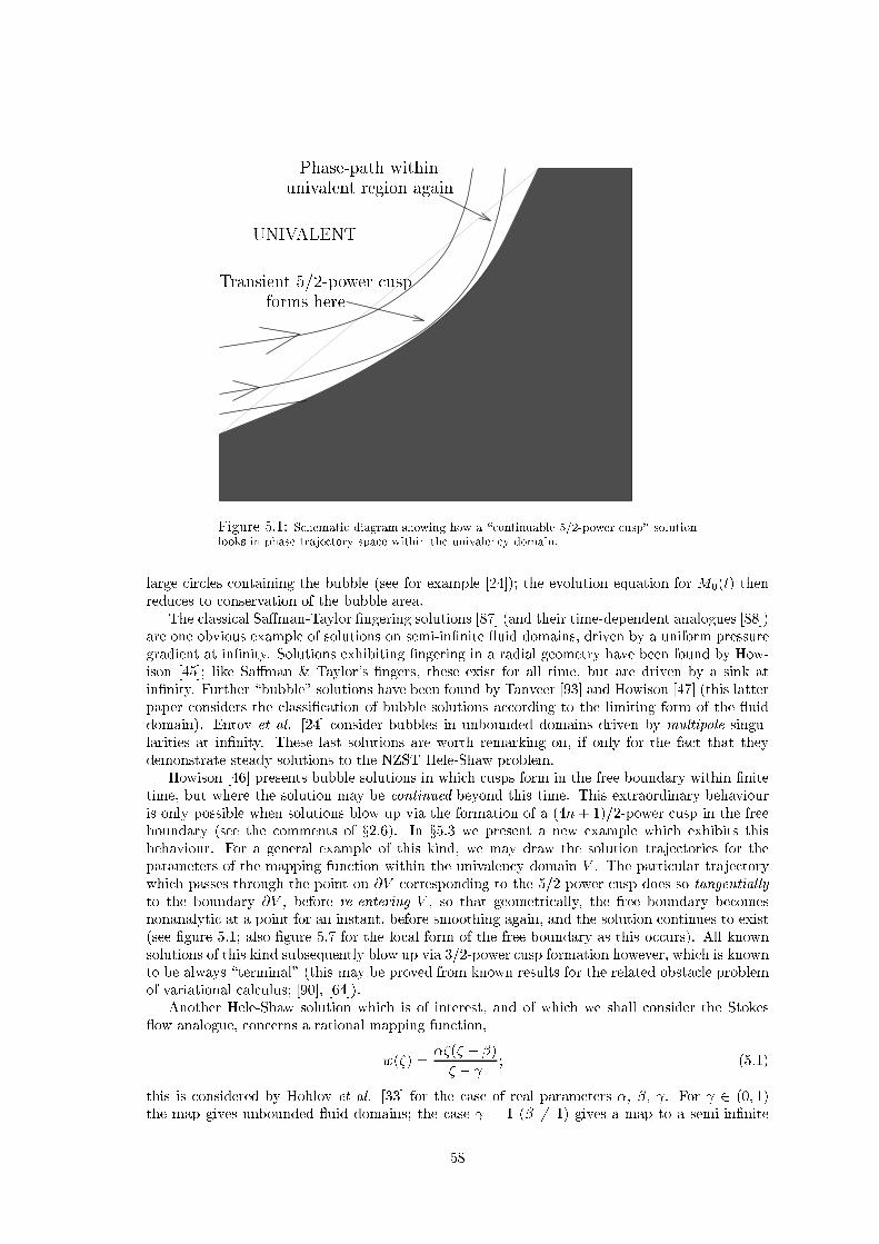
forms here
Transient 5/2-power usp
univalent region again
Phase-path within
UNIVALENT
Figure 5.1: S hemati diagram showing how a \ ontinuable 5/2-power usp" solution
looks in phase traje tory spa e within the univalen y domain.
large ir les ontaining the bubble (see for example [24℄); the evolution equation for M
0
(t) then
redu es to onservation of the bubble area.
The lassi al Sa�man-Taylor �ngering solutions [87℄ (and their time-dependent analogues [88℄)
are one obvious example of solutions on semi-in�nite uid domains, driven by a uniform pressure
gradient at in�nity. Solutions exhibiting �ngering in a radial geometry have been found by How-
ison [45℄; like Sa�man & Taylor's �ngers, these exist for all time, but are driven by a sink at
in�nity. Further \bubble" solutions have been found by Tanveer [93℄ and Howison [47℄ (this latter
paper onsiders the lassi� ation of bubble solutions a ording to the limiting form of the uid
domain). Entov et al. [24℄ onsider bubbles in unbounded domains driven by multipole singu-
larities at in�nity. These last solutions are worth remarking on, if only for the fa t that they
demonstrate steady solutions to the NZST Hele-Shaw problem.
Howison [46℄ presents bubble solutions in whi h usps form in the free boundary within �nite
time, but where the solution may be ontinued beyond this time. This extraordinary behaviour
is only possible when solutions blow up via the formation of a (4n+ 1)=2-power usp in the free
boundary (see the omments of x2.6). In x5.3 we present a new example whi h exhibits this
behaviour. For a general example of this kind, we may draw the solution traje tories for the
parameters of the mapping fun tion within the univalen y domain V . The parti ular traje tory
whi h passes through the point on �V orresponding to the 5/2-power usp does so tangentially
to the boundary �V , before re-entering V , so that geometri ally, the free boundary be omes
nonanalyti at a point for an instant, before smoothing again, and the solution ontinues to exist
(see �gure 5.1; also �gure 5.7 for the lo al form of the free boundary as this o urs). All known
solutions of this kind subsequently blow up via 3/2-power usp formation however, whi h is known
to be always \terminal" (this may be proved from known results for the related obsta le problem
of variational al ulus; [90℄, [64℄).
Another Hele-Shaw solution whi h is of interest, and of whi h we shall onsider the Stokes
ow analogue, on erns a rational mapping fun tion,
w(�) =
��(� � �)
� �
; (5.1)
this is onsidered by Hohlov et al. [33℄ for the ase of real parameters �, �, . For 2 (0; 1)
the map gives unbounded uid domains; the ase = 1 (� 6= 1) gives a map to a semi-in�nite
58

uid domain. The authors solve for the problem with a single point sink at the origin driving
the ow (the Stokes ow analogue we onsider is driven by a dipole singularity at the origin).
This situation di�ers from those mentioned above in that here, the driving singularity is at the
origin, whereas the previous ases were driven by pres ribed singularities at in�nity. The mapping
fun tion (5.1) is interesting be ause the points (�; ) on the boundary of the univalen y domain
in (�; )-spa e orrespond to uid domains having slits in them (along ar s of ir les).
Finally (for the Hele-Shaw problem) we mention the work of Ri hardson [79℄, where a limiting
pro edure is employed to solve for a problem on a semi-in�nite uid domain. The problem of a
point sink, pla ed o�- entre in an initially ir ular domain, is onsidered (the geometry of �gure
5.2 but with a di�erent driving singularity); the NZST version of this problem has re ently been
solved numeri ally in [55℄. For an initial ir le of radius r, entred at z = � < r (with the sink
at z = 0), the method outlined in x2.5 is used to �rst dedu e the orre t form of the mapping
fun tion, and then to solve the problem. The semi-in�nite domain limit is obtained by allowing
both r and � to tend to in�nity, whilst keeping the quantity r � � = k �xed. This pro ess yields
the solution for a point sink pla ed at the origin in the unbounded initial domain fx > �kg (so
here again we have a driving singularity at a �nite point within the ow domain). In x5.3 we
employ the same methods to solve the problem for a vortex dipole singularity at the origin, in the
same geometry.
We now onsider what results exist for the Stokes ow ase. Most of the work whi h has been
done on the unbounded domain problem involves steady solutions for �nite bubbles in (fully-
) in�nite uid domains, and was mentioned brie y in x1.4.2. One of the �rst papers of note
was Ri hardson [78℄ (1968), who solved the problem of a two-dimensional invis id bubble in the
ases of uniform shear, and pure straining, external ow. In a subsequent paper [80℄ he solved
the same problem for a paraboli external velo ity pro�le. In 1972, Bu kmaster [7℄ published
results for slender bubbles in three-dimensional axisymmetri slow vis ous ow (at small surfa e
tension), �nding bubble shapes whi h appeared to have usped ends; Antanovskii (though in two
dimensions) has also onsidered the formation of steady-state usped bubbles [3℄ and pointed
drops [4℄. Later work by Youngren & A rivos [101℄ (1976) gave agreement with Bu kmaster's
results for small values of surfa e tension, and with other experimental work for larger surfa e
tension values. Slender three-dimensional bubbles have been studied more re ently by Howell
[42, 43℄, in extensional ow, and with a time-dependent formulation (the above mentioned work
all being for steady ows).
Tanveer & Vas on elos [96℄ have re ently published results on the time evolution of two-
dimensional bubbles, where the motion is driven by a given external ow �eld at in�nity (whi h
may in lude a sour e/sink at in�nity, so that the bubble area an hange). Parti ular ases
onsidered are when the external ow is simple shear, and pure straining (as in Ri hardson [78℄,
but time-dependent), and they �nd a family of exa t solutions for a polynomial-type onformal
map. Three-dimensional time-dependent axisymmetri bubbles have also been studied by Nie
& Tanveer [70℄; in this paper and in [96℄ the possibility of \pin hing" is onsidered, where, for
a shrinking bubble, opposite sides of the bubble tou h before the bubble has vanished, and the
solution breaks down.
The work of [96℄ demonstrates that the ideas pioneered by Hopper [37, 38℄ and Ri hardson [82℄
for bounded uid domains, arry through to the unbounded domain (with �nite bubble) ase with
little modi� ation needed. However, very little work has been published relating to problems on
unbounded domains where the driving singularity is at some �nite point within the ow domain,
and, to our knowledge, all expli it solutions whi h have been found for su h ases are for the mu h
simpler, steady version. In fa t, the only notable ontribution to this problem of whi h we are
aware is the work of Jeong & Mo�att [52℄ (hen eforth J & M), who solve the steady problem for
a vortex dipole pla ed beneath a free surfa e in a semi-in�nite uid domain. This is intended to
model experiments performed in a large tank of uid, with two ounter-rotating ylinders pla ed
beneath the free surfa e. Antanovskii [2℄ generalises their work in two ways: �rstly, he allows a
variable interfa ial tension, to model the e�e t of surfa tant, and se ondly, he assumes ea h of the
ounter-rotating ylinders to be represented by a separate vortex singularity in the ow (although
an exa t analyti al solution is only found in the limit in whi h these two vorti es merge to form
59

Fluid
� r + ��(r � �) x
y
Figure 5.2: The geometry for the problem of a dipole pla ed o�- entre in a ir le.
a single vortex dipole, as onsidered by J & M).
Our idea was to present a time-dependent version of the work of J & M (whi h would hopefully
tend to their solution as t! 1), sin e no solutions to problems of this kind exist in the urrent
literature. As we shall see though, this is far from trivial, involving ompli ations of the kind
hinted at in x5.1. Before onsidering su h a generalisation, we will brie y review the analysis of
J & M, but before we do this we solve the orresponding ZST Hele-Shaw problem, whi h turns
out to be mu h more straightforward than the Stokes ow problem.
5.3 The Hele-Shaw dipole problem
In this se tion we show that the ZST Hele-Shaw version of the J & M dipole problem an be
solved without diÆ ulty. It is worth doing this for two reasons; �rstly, it represents an interesting
new solution for Hele-Shaw, being one whi h exhibits the \transient 5/2-power usp" behaviour
referred to earlier, and furthermore, it has the driving singularity at a �nite point within the uid
domain (as in the Stokes ow literature, most in�nite-domain Hele-Shaw solutions have driving
singularities at in�nity). Se ondly, it illustrates the use of the pro edure outlined in x2.5, for
dedu ing the form of the mapping fun tion that is needed for a parti ular geometry.
The analysis is a simple adaptation of that given in Ri hardson [79℄, where the same geometry is
assumed (i.e. an initially ir ular domain, with an o�- entre singularity; see �gure 5.2) but instead
a point sink drives the ow. The dipole singularity in our example for es a more ompli ated
mapping fun tion than in that paper; hen e the solution we obtain has a di�erent stru ture|all
solutions in [79℄ blow up in �nite time via formation of a single 3/2-power usp.
Re all the result (2.10) linking the time evolution of the S hwarz fun tion, g(z; t), to the
omplex potential, W(z), of the ow. For the ase of a vortex dipole singularity of strength M at
the origin, in the sense of �gures 5.2 and 5.3, the only singularity of W(z) is at z = 0, this being
W(z) = �
M
z
+O(1) as z ! 0:
60

It follows from (2.10) that, near the origin, the S hwarz fun tion varies a ording to
�g
�t
= 2
dW
dz
=
2M
z
2
+O(1) as z ! 0; (5.2)
so that, de omposing the S hwarz fun tion a ording to (2.25), the singular part must satisfy
g
e
(z; t) = g
e
(z; 0) +
2Mt
z
2
:
The S hwarz fun tion for a ir ular initial domain, with entre at z = � and radius r > �, is
given in [79℄ (and in any ase is trivial to �nd) as
g(z; 0) = �+
r
2
z � �
; (5.3)
hen e for t > 0 the singular part of the S hwarz fun tion is given expli itly by
g
e
(z; t) =
r
2
z � �
+
2Mt
z
2
: (5.4)
Let the point d(t) within fj�j � 1g map to the point � in the physi al domain, w(d) = � (we
know that the origin maps to the origin, and that the mapping fun tion is analyti on the unit
dis ). The relation (2.27) then tells us that the omplex onjugate mapping fun tion �w(1=�) has
to have a double pole at � = 0, a simple pole at � = d, and no other singularities. Sin e w(0) = 0,
�w(1=�) must also vanish at in�nity, and hen e must be of the form
�w(1=�) =
a
�
2
+
B
�
+
C
� � d
; (5.5)
so that assuming a; B; C; d 2 R, whi h amounts to assuming symmetry about the x-axis, we
have
w(�) = a�
2
+B� +
C�
1� d�
: (5.6)
To determine the parameters a; B; C and d in (5.6), we need to mat h singularities within the unit
dis in equation (2.12). This requires a straightforward lo al analysis at ea h of the singularities,
and yields the three algebrai equations,
a(B + C)
2
= 2Mt; (5.7)
B(B + C)
3
a+ Cd
= �4Mt; (5.8)
Cw
0
(d) = C
�
2ad+B +
C
(1� d
2
)
2
�
= r
2
: (5.9)
The fourth equation needed omes from the requirement w(d) = � (whi h embodies the fa t that
the singularities of the S hwarz fun tion remain �xed in the physi al plane for Hele-Shaw ow),
ad
2
+Bd+
Cd
1� d
2
= �: (5.10)
These equations are seen to satisfy automati ally the orre t initial onditions for the geometry
(0), namely
a(0) = 0 = B(0); C(0) = r
�
1�
�
2
r
2
�
; d(0) =
�
r
:
Note that the system is simpler if we repla e (5.8) by ((5.8) + 2� (5.7)), i.e.
2a(a+ Cd) +B(B + C) = 0: (5.11)
61

Dipole
x
y
Fluid
�k
Figure 5.3: The geometry for the dipole-in-a-half-spa e problem.
Solving for a; B; C and d gives the evolution of the uid domain until su h time as the solution
breaks down, with loss of univalen y of the mapping fun tion. We do not solve (5.7){(5.10)
expli itly, however, be ause we are primarily interested in the in�nite domain limit (�gure 5.3).
In addition, the system (5.7){(5.10) is spe i� to an initially- ir ular geometry (or an initially-
at geometry in the unbounded domain limit), and it is lear that with the mapping fun tion
(5.6), we may onsider the evolution of more general initial domains than this. Sin e we are now
proposing a de�nite form, (5.6), for w(�; t), the governing equations for the more general ase are
best obtained using the method outlined below equation (2.12) in x2.3 (and illustrated in x2.4).
We know that (5.2) represents the only singular behaviour of �g=�t in (t). We also know
that g(z) � �w(1=�) (equation (2.12)), whi h by (5.5) has singularities at points � = 0 and � = d
within the unit dis . Hen e, expanding the mapping fun tion to �nd � as a fun tion of z in the
neighbourhood of these points, we may �nd the lo al form of g(z) at both points z = 0, z = w(d),
and use (5.2) to get the o.d.e.'s governing the oeÆ ients. Near z = 0 = � we have
� =
z
w
0
(0)
�
w
00
(0)z
2
2w
0
(0)
3
+O(z
3
);
so that a lo al analysis here yields
g(z) =
aw
0
(0)
2
z
2
+
aw
00
(0) +Bw
0
(0)
z
+O(1):
Hen e, mat hing singularities in (5.2),
d
dt
(aw
0
(0)
2
) = 2M; (5.12)
aw
00
(0) +Bw
0
(0) = onst. = k
1
: (5.13)
Near � = d,
� � d =
z � w(d)
w
0
(d)
+O((z � w(d))
2
);
so by (2.12) and (5.5),
g(z) =
Cw
0
(d)
z � w(d)
+O(1);
62

and (5.2) gives the two equations
w(d) = onst. = �; (5.14)
Cw
0
(d) = onst. = r
2
: (5.15)
Equations (5.7), (5.11), (5.10) and (5.9) are easily seen to be a spe ial ase of equations (5.12){
(5.15).
2
The onstants in (5.14) and (5.15) are arbitrary; we write them as � and r
2
to onform
with the spe ial ase onsidered �rst. We are justi�ed in assuming that the onstant in (5.15)
is positive, sin e we are assuming that the positive real axis within the unit dis maps onto the
positive real axis in the uid domain.
Taking the in�nite domain limit of the problem involves letting r and � tend to in�nity whilst
keeping r � � = k �xed. Equations (5.12) and (5.13) have trivial limits,
a(B + C)
2
= 2Mt+ onst.; (5.16)
2a(a+ C) +B(B + C) = k
1
; (5.17)
whilst a areful analysis of equations (5.14) and (5.15) shows that they redu e to the single
ondition
C � 2(a+B) = 2k: (5.18)
Geometri ally this last equation is what we expe t; it says that asymptoti ally, the free boundary
is jyj ! �1, x � �k. It is easily veri�ed that the solution represented by equations (5.16){(5.18)
gives a velo ity �eld whi h tends to zero at in�nity, whi h we learly require for a realisti solution.
To see by what possible means this more general solution may blow up, we must onsider the
subset of (a;B;C)-parameter spa e on whi h the map with d = 1 is univalent. For this purpose
it is simplest to rewrite the map as
w(�) = a
�
�
2
+ b� +
�
1� �
�
; (5.19)
so that in fa t we only need onsider univalen y of the map in (b; )-parameter spa e. The only
drawba k of writing the map this way is that the limit a ! 0 is degenerate; maps whi h pass
through or start from su h on�gurations must have ! �1 (b an either be ome unbounded or
remain O(1))|the \initially at" on�guration is one su h ase, as are any solutions whi h pass
through at on�gurations.
We may determine the univalen y domain V in (b; )-parameter spa e by looking for boundary
urves on whi h w
0
(e
i�
) = 0 for real � (the ondition that the free boundary has a usp), and
also urves on whi h w(e
i�
) = w(e
�i�
) for real, nonzero � (the ondition that the free boundary is
self-interse ting, using the symmetry of the domain). We omit the analysis, whi h is not diÆ ult,
but rather tedious. The result is that V is split into two parts, in > 0 and < 0 (see �gure 5.4;
the line = 0 is not relevant to the present dis ussion, sin e it represents bounded uid domains,
and our solution traje tories annot rea h it). That part of V in > 0 is bounded by the lines
4b+ = 8 and = 0;
whilst the part in < 0 is bounded by
b+ + 4 = 0; = 0;
and the parabola
+
�
b
2
+ 1
�
2
= 0;
2
Note that the system (5.12){(5.15) ould have been obtained working wholly in the �-plane, using the ZST
version of (3.38).
63

−6 −4 −2 0 2 4 6 8−25
−20
−15
−10
−5
0
5
10
b
= 0 = 0
NONUNIVALENT
UNIVALENT
UNIVALENT
4b+ = 8
b + + 4 = 0
Overlapping
Two 3/2-power usps
(lima� ons)
Single 3/2-power usp
Bounded uid domains
free
boundary
+
�
b
2
+ 1
�
2
= 0
Figure 5.4: The univalen y domain in (b; )-spa e for the mapping fun tion (5.19).
64

-10 -7.5 -5 -2.5 2.5 5 7.5 10
-15
-10
-5
5
10
15
-10 -7.5 -5 -2.5 2.5 5 7.5 10
-15
-10
-5
5
10
15
-10 -8 -6 -4 -2 2
-1.5
-1
-0.5
0.5
1
1.5
-2.75 -2.5 -2.25 -2 -1.75 -1.5 -1.25 -1
-0.2
-0.15
-0.1
-0.05
0
0.05
0.1
0.15
0.2
Fluid Fluid
Fluid Fluid
Air
Air Air
AirAir
(1) (2)
(3b)(3a)
Figure 5.5: Typi al free boundaries generated by points (b; ) on the boundary of the univalen y domain (�gure
5.4). The dipole is situated at the origin in ea h ase, and is su h that the x-axis is a streamline in the positive
sense. (1) has a = 1, b = 1, = 4, and has a single usp in the free boundary; (2) has a = �1, b = 1, = �5, and
has two usps in the free boundary, and (3a) has a = �1, b = 4, = �9, and shows the free boundary beginning
to overlap itself. (3b) is an enlargement of the trapped air bubble in (3a).
65

whi h meets the line b+ + 4 = 0 at the point (2
p
3;�(4 + 2
p
3)).
With our \normalisation ondition" that the positive real axis in the �-plane should map to
the positive real axis in the z-plane, we require a(0) > 0 for solutions in > 0, and a(0) < 0
for solutions in < 0. Geometri ally, in the upper part of V , the line 4b+ = 8 orresponds to
loss of univalen y via formation of a single 3/2-power usp at the point z = w(�1) on � (�gure
5.5 (1)). The line = 0 is the �nite domain limit in whi h the uid domain is a ardioid ( f the
lima� on example of x2.4). In the lower part of V , the line b+ + 4 = 0 gives free boundaries �
having two 3/2-power usps, symmetri ally pla ed about the x-axis (�gure 5.5 (2)). Along the
paraboli portion of �V the free boundary is nonanalyti due to self-interse tion (�gure 5.5 (3)),
ex ept for the isolated point (6;�16), where � has a single 5/2-power usp|at this point the
parabola is a tually tangent to the line 4b + = 8 (whi h formed part of �V in the upper half
plane, > 0). Figures 5.4 and 5.5 should larify the above explanation.
The analogues of equations (5.16){(5.18) for the modi�ed mapping fun tion (5.19) are:
a
3
(b+ )
2
= 2Mt+ onst.; (5.20)
2(1 + ) + b(b+ ) =
k
1
a
2
; (5.21)
� 2(1 + b) =
2k
a
; (5.22)
eliminating a between the last two yields the solution traje tories in (b; )-spa e as
2 + b
2
+ (2 + b)
(1 + b� =2)
2
= �;
for various onstants �, determined by the initial onditions (�gure 5.6). This equation learly
represents some kind of oni se tion, depending on the value of � hosen. Changing to axes
aligned with the prin ipal axes, it an be rearranged into the form
�
b�
2
+ 1 + 3�
�
2
� 4�
�
b+
4
+ 1
�
2
= 9�(1 + �);
where � = 1=(3�+ 1). From this it is lear that for 0 < � < 1 the phase paths are bran hes of
hyperbolae, with asymptotes
2
(1�
p
�) = b(1� 2
p
�) + 1 + 3�� 2
p
� ;
(so the gradient of these asymptotes is 2(1 � 2
p
�)=(1 �
p
�)). The two sets of bran hes are
separated by the � = 0 (straight line) path,
b�
2
+ 1 = 0:
A positive value of � does not uniquely spe ify a solution path then, sin e there are two possible
bran hes. This is not a problem, however, be ause the value of � is determined by the initial
onditions, and obviously the free boundary has to evolve in a ontinuous manner, so we must
stay on the parti ular path on whi h we start.
Values of � between �1 and �1 give ellipti al phase paths, � = �1 being the value at whi h
the family of ellipses ollapses to the single point (0;�4), whi h a tually lies on the boundary
�V . There are no real phase traje tories for � 2 (�1; 0). The limit � ! �1 orresponds to the
original parameter � approa hing the value �
1
3
from above or below; the limiting phase path is a
parabola with equation
Y
2
=
3
2
�
X �
3
2
�
; (5.23)
where X = 1 + b� =2 and Y = 1 + b+ =4 are the o-ordinates along the prin ipal axes of the
family of oni s.
66

−6 −4 −2 0 2 4 6 8−20
−15
−10
−5
0
5
10
b
� = 0
"5/2- usp" phase path for � = �5
tangent to boundary at (6;�16)
Paraboli path � = �1
separating ellipses (� < 0)
from hyperbolae (� > 0)
Degenerate phase path
for � = �1, at (0;�4)
� = �2
� = �3
"Separatrix"
� = 1 path
"Separatrix"
� = 0
Figure 5.6: The phase diagram (within the univalen y domain) for the Hele-Shaw dipole problem.
67

2 4 6 8 10
-35
-30
-25
-20
-15
-10
-5 -4 -3 -2 -1
-0.4
-0.3
-0.2
-0.1
0.1
0.2
0.3
0.4
-3.5 -3 -2.5 -2 -1.5 -1 -0.5 0.5
-0.2
-0.1
0.1
0.2
-3.5 -3 -2.5 -2 -1.5 -1 -0.5 0.5
-0.4
-0.2
0.2
0.4
NONUNIVALENT REGION
Fluid Fluid Fluid
(a) (b) ( )
Line b+ + 4 = 0
(single 3/2-power usp)
Phase path inside V here (b)
Ultimate blow-up
with two 3/2-power
usps forming ( )
Curve =
�
b
2
+ 1
�
2
Point where 5/2-power
usp forms (a)
Phase
traje tories
Figure 5.7: Enlargement of the transient 5/2-power usp formation. Pi tures (a), (b) and ( ) illustrate how the
free boundary passes through the 5/2-power usped on�guration (a), to a smooth boundary (b), before ultimately
blowing up with two 3/2-power usps ( ).
68

The phase diagram within the univalen y domain is shown in �gure 5.6. The arrows on the
phase paths are for positive values of the dipole strength M (so the dipole has the sense in �gure
5.3); if the dipole is reversed, so are these arrows. Points to note about the phase diagram are:
� The existen e of the ellipti al solution traje tory for � = �5, whi h is tangential to the
paraboli part of �V at the point (6;�16), and re-enters V immediately (�gure 5.7). As
dis ussed in x5.2, this orresponds to the appearan e, and subsequent immediate disappear-
an e, of a 5/2-power usp in �. Note that this traje tory rea hes the boundary b+ +4 = 0
of �V shortly afterwards, so that the solution does ultimately blow up with the formation
of two 3/2-power usps in �.
� The existen e of the \degenerate" phase path b = 0; = �4, (� = �1), whi h lies on �V .
This annot represent a solution, however, sin e equations (5.20){(5.22) annot be solved
for a(t) if b and are onstant.
� The paraboli phase path (� ! �1, or � = �1=3), separating the ellipti al paths in the
lower part of V , from the bran hes of the hyperboli paths in that part of V .
In the lower part of V , the paths whi h \go o� to in�nity" whilst remaining within V are
those hyperboli paths for 0 < � < 1 whi h lie to the right of the \separatrix" 1 + b = =2 (the
� = 0 path), and those for 0 < � < 1=4 to the left of the separatrix.
For the paths lying to the right of the separatrix, � = 1 (� = 0) gives the hyperbola whi h has
an in�nite-gradient asymptote. The orresponding asymptotes of the hyperbolae for 0 < � < 1
have gradients lying in the range 2 to 1 (2 being the gradient of the separatrix), whilst those for
� > 1 will have asymptotes with negative gradient. These � > 1 hyperbolae will thus interse t the
paraboli part of �V before b and be ome in�nite, and solution breakdown via self-overlapping
of the free boundary o urs. The hyperbolae for 0 < � < 1, whi h lie between the � = 0 separatrix
and the � = 1 path, have orresponding bran hes in the upper part of V . What happens with
these solutions is that we rea h = �1 within �nite time, then reappear on the orresponding
bran h at = +1 in the upper part of V . We have to be areful, sin e there are two possible
bran hes for a parti ular value of �, but a little thought tells us that the \ orresponding bran h"
is the bran h having the same value of �, but now lying to the left of the separatrix in the upper
half of V , sin e the free boundary shape must hange in a ontinuous manner.
This transition from = �1 to = +1 is simultaneous with a passing through the value
zero. Only if b remains O(1) as this happens will we have the free boundary passing through the
ompletely at on�guration, whi h is the spe ial ase we onsidered �rst. This will be exa tly
the hyperboli path whose asymptote has in�nite gradient, i.e. the � = 1 (or � = 0) path, along
whi h b! �2 as �! �1.
For the paths lying to the left of the separatrix in the lower half of V , � = 1=4 is the value for
whi h one of the asymptotes of the hyperbola has zero gradient. Phase paths for 0 < � <
1
4
will
thus extend to in�nity without leaving the domain V ; as above, this will o ur within �nite time,
and the solution is ontinued by reappearing at in�nity on the orresponding path in the upper
part of V , whi h will here lie to the right of the � = 0 separatrix. It an be seen, by onsidering
the arrows on the phase paths in the upper half of V , that all solutions exhibiting this kind of
behaviour will ultimately blow up with formation of a 3/2-power usp in the free boundary at the
point w(�1).
The paraboli phase path is ex eptional in that it has no omponent in the upper part of
V . The solution represented by this traje tory blows up within �nite time when it interse ts the
paraboli part of �V , at the point (b; ) = (21:2328;�134:941), with self-interse tion of the free
boundary.
We have been able to analyse the possible kinds of behaviour, without solving expli itly for
(a; b; ). A omplete des ription would involve solving (5.20){(5.22), but little would be gained
by doing this, sin e the above working aptures all the essentials, and ertainly all the interesting
aspe ts of the problem.
As an aside, we omment that the analysis may be extended to the ase of a general multipole
singularity at the origin (as onsidered by Entov et al. [24℄). For a multipole of order n, the
69

omplex potential has the behaviour
W(z) = �
M
z
n
+O(1) as z ! 0;
so that the singular part of the S hwarz fun tion is given by
g
e
(z; t) =
r
2
z � �
+
2nMt
z
n+1
;
instead of (5.4). Thus in this ase, by (2.27), the omplex onjugate mapping fun tion must have
a pole of order (n+1) at � = 0 and a simple pole at � = d as its only singularities within the unit
dis , and must vanish at in�nity. The mapping fun tion for this ase will therefore be given by
w(�) =
n+1
X
r=1
a
r
�
r
+
C�
1� d�
; (5.24)
(with d = 1 in the unbounded domain limit). The more ompli ated form of this fun tion will
allow for more varied behaviour of solutions, but for larger values than n = 1 it is mu h more
diÆ ult to determine the univalen y region for the map in parameter spa e.
5.4 The Stokes ow dipole problem
5.4.1 Review of Jeong & Mo�att's steady solution
Before onsidering time-dependent possibilities, we �rst review the steady Stokes ow dipole
problem as solved by J & M [52℄, sin e this was our original motivation for studying problems on
unbounded domains with �nite driving singularities. This problem models experiments performed
(at low Reynolds number) in a large tank of vis ous uid, with two ounter-rotating ylinders
pla ed beneath the free surfa e. Above a ertain riti al rate of rotation of the ylinders, a steady
state was qui kly attained in whi h the free surfa e of the uid above the ylinders had an apparent
usp. It is this steady-state on�guration whi h J & M's solution des ribes.
The presentation we give here is slightly di�erent to theirs, sin e we use the te hniques and
onventions of this thesis; however in all essentials it is the same. We use the form of the governing
equations given in x3.2.1; in the simpler time-independent ase here, equation (3.26) integrates to
X (�) + �w(1=�)�(�) = 0; (5.25)
whi h is just the ondition that the free boundary be a streamline, analyti ally ontinued to hold
globally. �(�) is given (from (3.15)) by
�(�) =
T
4�
[f
+
(0)� 2f
+
(�)℄�w
0
(�; t) +
w
0
(�)
w
0
(0)
A(1� �
2
); (5.26)
where we have assumed �(�) to be bounded at the origin (with limit A), whi h will be the ase if
we have a pure vortex dipole at the origin. We have also assumed that A is real, whi h is equivalent
to requiring the geometry to be symmetri about the x-axis (if we also have a onformal map with
real parameters). Thus our geometry is J & M's, rotated through 90
0
, and the free boundary at
in�nity will be x = onstant, with the uid o upying the region to the right of this boundary
(see the Hele-Shaw de�nition sket h, �gure 5.3). The dipole is taken to be situated at the origin,
and the onformal map is subje t to the usual onditions w(0; t) = 0, w
0
(0; t) > 0.
Some point on the unit ir le must map to in�nity; with the above restri tions, this an only
be the point � = 1. The geometri al onstraint that the free boundary be asymptoti ally at
for es the behaviour
w(�) =
�
1� �
+O(1) as � ! 1;
70
for some real positive �, and there are no other singularities of w(�) within the unit dis . Con-
sideration of the dipole behaviour at � = 0 requires (using (5.25))
�w(1=�) = �
M
Aw
0
(0)�
+O(1) as � ! 0; (5.27)
so that the mapping fun tion must be of the form
3
w(�) = �� +
��
1� �
: (5.29)
For this map, the free boundary at in�nity is given by
x = ��
�
2
; jyj ! 1;
and sin e we must be able to spe ify the depth of the dipole beneath this asymptoti free surfa e,
we may insist
� =
�
2
� 1
without loss of generality (taking this dipole depth to be 1). There are now only two unknown
quantities, the parameter �, and A � �(0). The behaviour at the dipole gives A in terms of �,
sin e by (5.27) and (5.29) we must have
�A = �
M
w
0
(0)
� �
M
3�+ 2
:
We �nally have to satisfy the ondition that the ow be stagnant at in�nity, where the e�e t of
the dipole annot be felt. The most general behaviour of �(z) and �(z) allowing this is
�(z) = �
p
1
4�
z + � +O(1=z); (5.30)
�(z) = z +O(1); (5.31)
both holding as jzj ! 1; this may be seen from (3.2) and (3.3) (p
1
denotes the pressure �eld at
in�nity). For this parti ular ase we take p
1
= 0; this is ne essary if we are to get the orre t
balan e in (5.25) at in�nity, be ause the map (5.29) satis�es
�w(1=�) � �w(�) (5.32)
at leading order, as � ! 1. With our symmetri geometry, the onstant will be real. Thus, if
we an ensure that �(�) remains bounded as � ! 1, denoting this limit by , equation (5.25) will
automati ally ensure that the se ond of the `stagnant ow' onditions is satis�ed.
Writing � = 1� �, (5.26) gives the asymptoti behaviour of �(�) near � = 1 as
�(�) =
T�
4��
2
(f
+
(0)� 2f
+
(1))�
1
�
�
T�
4�
(f
+
(0)� 2f
+
(1)� 2f
0
+
(1))�
2A�
w
0
(0)
�
+O(1):
3
We note in passing that the analysis is easily generalised to the ase of a general multipole singularity at the
origin, for whi h the fun tion X (�) has the behaviour
X (�) =
M
�
n
w
0
(0)
n
+O
�
1
�
n�1
�
; as � ! 0: (5.28)
This would ne essitate a pole of order n at � = 0 in �w(1=�), giving the general form of the map as
w(�) =
n
X
r=1
�
r
�
r
+
��
1� �
:
71

(All quantities appearing in this expression are either given, or else are known fun tions of �). It
is easy to see from the de�nition (3.8) that
f
+
(0)� 2f
+
(1) =
i
2�
Z
2�
0
sin � d�
jw
0
(e
i�
)j(1� os �)
;
whi h is identi ally zero, by a simple symmetry argument. Thus the singularity of order 1=�
2
in
�(�) vanishes automati ally, and we need only impose the ondition
T
4�
f
0
+
(1) +
A
w
0
(0)
= 0;
to remove the order 1=� singularity. Use of (3.8) redu es this to
�(0) =
Tw
0
(0)
16��
Z
2�
0
1
jw
0
(e
i�
)j
d�
(1� os �)
;
whi h is the single ondition needed to omplete the solution. For detailed dis ussion of the
results, and omparison of the free boundary shape with experiment, see [52℄.
5.4.2 The time-dependent problem
Having seen how the steady problem works, we onsider how we might generalise the analysis to
�nd a time-dependent solution. Re alling the omments of x5.1, we annot expe t to �nd su h a
solution unless we allow the singularity to move relative to the uid mass, and we �nd that this
is indeed the ase, at least when we assume �(0) = 0.
We begin by observing that, if su h a solution exists, it must be realisable as the limit of
a dipole-in- ir le problem, su h as we solved for Hele-Shaw ow in x5.3. Motivated by this, we
attempt the Stokes ow problem, using the method outlined in x3.7 to �nd the onformal map.
As ommented in x3.6.2, if a onformal map gives a solution to the ZST time-dependent problem,
the same map will also work for the NZST problem, hen e we onsider the easier ZST ase. For
a pure dipole singularity at the origin, we require �(�) to be bounded there, but do not yet know
whether we may assume it to be zero. (Given that �(0) turned out to be nonzero for the steady
problem of x5.4.1, we an hardly expe t to �nd a time-dependent solution for whi h it is zero,
but it is instru tive to see what happens when we onsider both ases.) We onsider the simpler
situation in whi h �(0) � 0 �rst.
In this ase, and with a dipole singularity at the origin, the fun tion H
e
(�; t) is given by (3.63),
so we need to determine H
e
(�; 0). The S hwarz fun tion of the initial domain is exa tly as for
the Hele-Shaw problem, and is given by (5.3); from this the fun tions g
e
(z; 0) and h
e
(z; 0) are
immediate as
g
e
(z; 0) =
r
2
z � �
; h
e
(z; 0) = r
2
log(z � �):
If d is the (unique) point within the unit dis su h that w(d; 0) = �, then we must have
H
e
(�; 0) = r
2
log(� � d); (5.33)
so that for the ase of a dipole singularity driving the ow we have
H
e
(�; t) = r
2
log(� � d)�
M�(t)
�
;
by (3.63), with �(t) as de�ned there. Sin e H
0
(�) = w
0
(�) �w(1=�), the singular part of this
ombination within the unit dis is given by
[w
0
(�) �w(1=�)℄
sing
=
r
2
� � d
+
M�(t)
�
2
:
72

These singularities must ome from the term �w(1=�), the mapping fun tion being analyti on the
unit dis . Hen e, if a solution to the problem as stated exists, the orre t mapping fun tion must
be su h that �w(1=�) has a double pole at the origin, and a simple pole at some (�xed) point � = d,
as its only singularities within the unit dis . It an have no singularities outside the unit dis
sin e this would entail w(�) being nonanalyti on j�j < 1. It follows that w(�) must be of the
form
w(�) = a�
2
+ b� +
�
1� d�
; (5.34)
for some time-dependent parameters a; b and , whi h is exa tly the map whi h was used for the
Hele-Shaw solution of x5.3.
4
This will always be the ase with the assumption �(0) = 0; if a
Stokes ow solution of this kind exists, it must be su h that the mapping fun tion is the same as
for the orresponding Hele-Shaw solution.
To �nd the equations governing the evolution of the parameters in (5.34), we must return to
(3.29) and make a quantitative omparison of singularities at � = 0 and � = d. The appropriate
behaviour of X
0
(�) on the right-hand side of (3.29) is X
0
(�) = �M=(�
2
w
0
(0)) +O(1) near � = 0,
whilst X
0
(�) must be regular at � = d. Mat hing at � = 0 gives the equations
d
dt
(a(b+ )) =
2M
b+
; (5.35)
2a(a+ d) + b(b+ ) = onst: = 0; (5.36)
while eliminating the singularity at � = d yields
d = onst: =
�
r
; (5.37)
w
0
(d) =
�
2ad+ b+
(1� d
2
)
2
�
= onst. = r
2
: (5.38)
Note that equations (5.36) and (5.38) are exa tly the same as (5.11) and (5.9) for the Hele-Shaw
problem; (5.35) is analogous to (5.7), and (5.37) is analogous to (5.10). The onstan y of d
here emerged naturally as a onsequen e of the solution (3.63), but in any ase ould have been
assumed a priori by the omment of x3.6.2 that the singularities of the S hwarz fun tion must
remain �xed in the �-plane. The values of the onstants on the right-hand sides of these equations
were obtained from the initial onditions on the map ne essary to give the ir le of radius r entred
at z = �, namely
(0) = r(1�
�
2
r
2
); b(0) = 0 = a(0); d(0) =
�
r
;
the ondition on d(0) gives the value of d for all time. We have the three equations (5.35), (5.36)
and (5.38) to solve for the fun tions a(t), b(t) and (t), whi h is a well-determined system. At
�rst sight then, it seems that everything is leading to a solution of the physi al problem; however
when we onsider the large domain limit (as we did for the analogous Hele-Shaw problem), we
en ounter problems, �nding that the entire uid mass translates uniformly relative to the (�xed)
dipole (or vi e-versa, if we subtra t o� this translational velo ity from the solution).
To see this expli itly, we take the same limit as in x5.3, letting r !1, �!1, while keeping
(r � �) �xed at k (this being the problem of a dipole pla ed at z = 0 in the half-spa e of uid
fx > �kg). In this limit d approa hes the value 1, and (0) approa hes 2k. Equation (5.35) still
stands, and (5.36) has the obvious limit obtained by setting d = 1. A leading-order balan e is
a hieved in (5.38) only if (t) assumes the onstant value, 2k. As the limit is approa hed, it is
prudent to look at what is happening far from the dipole, sin e physi ally the free surfa e ought
4
As ommented there (and again in footnote (3)), we ould equally well onsider a multipole singularity at the
origin. For a multipole of order n the fun tion X (�) has the behaviour of (5.28); this would also lead us to the
same map as for Hele-Shaw, namely (5.24).
73
to be undisturbed ( at) as x ! �1, and the velo ity �eld ought to be zero at in�nity. For the
ZST problem with �(0) = 0, the velo ity �eld is given by (C.1) with T = 0, that is,
2(u� iv) = �w
t
(1=�) + w
t
(�) +
w
0
t
(�)
w
0
(�)
�
�w(1=�)� w(�)
�
: (5.39)
The map for the in�nite domain limit is
w(�; t) = a�
2
+ b� +
�
1� �
;
with initial onditions as before ex ept that now (0) = 2k. Sin e � = 1 maps to in�nity, we write
� = 1� � for small � 2 C and examine the velo ity �eld (5.39). The various expressions are found
to be
�w(1=�) = �
�
+ (a+ b) + �(2a+ b) +O(�
2
);
w(�) =
�
+ (a+ b� )� �(2a+ b) +O(�
2
);
�w
t
(1=�) = �
_
�
+ (_a+
_
b) + �(2 _a+
_
b) +O(�
2
);
w
t
(�) =
_
�
+ (_a+
_
b� _ )� �(2 _a+
_
b) +O(�
2
);
w
0
t
(�)
w
0
(�)
=
_
+
�
2
2
h
(2 _a+
_
b)� _ (2a+ b)
i
+
2�
3
2
(a _ � _a ) +O(�
4
);
ombining these gives the velo ity at large distan es from the dipole as
u� iv = �
_
�
+ (_a+
_
b) +O(�):
The leading-order term here vanishes, sin e we already know is a onstant (equal to 2k) from
the balan e of terms in (5.38). We also require
a(t) + b(t) = onst. = 0;
ombined, these two onditions give � 2(a+ b) = 2k, f (5.18), whi h is exa tly the requirement
that the asymptoti free boundary at in�nity be �xed relative to the dipole. These onditions
are learly in ompatible with equations (5.35) and (5.36) (with d = 1 in the latter). Insisting
that (5.35) and (5.36) hold, as they must ertainly do to �t the onditions at the dipole, the best
we an then do is to take (t) to be onstant, giving bounded, but nonzero, velo ity at in�nity.
Physi ally, this orresponds to the entire uid mass translating with speed a(t) + b(t) relative to
the �xed dipole, whi h is a highly arti� ial geometry. The unrealisti nature of this large domain
limit implies that the �nite domain solution represented by the system (5.34){(5.38) must also be
arti� ial, otherwise it would give a sensible limit.
5
The una eptability of this parti ular solution is a onsequen e of the assumption �(0) = 0
whi h was made, sin e if a solution exists to the problem of a pure dipole in this geometry, �(0) is
ne essarily regular at the origin, but need not vanish there (see the omments following (3.14) in
x3.1). We therefore onsider what form the mapping fun tion must take in this ase. The relevant
governing equations for the S hwarz fun tion are now (3.57) and (3.54); by the remarks following
(3.57) the solution for H
e
(�; �) may be written down from (3.58) as
H
e
(�; �) =
C
0
�
log � �
1
�
Z
�
0
(C
0
+M�=A(�
0
)) d�
0
tanh(�
0
� � + tanh
�1
�)
�
1
�
f(tanh
�1
� � �)
�
1
�
Z
�
0
C
1
(�
0
) d�
0
;
5
As an aside, we note that if we onsider the simpler problem of a point sink singularity in this geometry, the
same unphysi al result is obtained.
74

where C
0
and C
1
are, respe tively, the zeroth and �rst \moments", and f is a fun tion to be
determined. Note that we are now working with the s aled time variable � , de�ned in (3.51), and
that sin e we have no point sink at the origin, the \moment" C
0
is a onstant equal to the area of
the uid domain (�r
2
here). We have initial onditions (5.33) as before, from whi h the fun tion
f is seen to be
f(�) = �r
2
log(tanh �)� �r
2
log(tanh � � d):
After simplifying and rearranging, the solution for H
e
be omes
H
e
(�; �) = r
2
log � � r
2
log(� � tanh �) + r
2
log(� � tanh(� + tanh
�1
d))
�r
2
Z
tanh �
0
(1� �x) dx
(� � x)(1� x
2
)
�M
Z
tanh �
0
(1� �x) dx
A(� � tanh
�1
x)(� � x)(1� x
2
)
;
(plus some fun tion of � , irrelevant to the dis ussion). Hen e,
H
0
e
(�; �) =
r
2
�
�
r
2
� � tanh �
+
r
2
� � tanh(� + tanh
�1
d)
+r
2
Z
tanh �
0
dx
(� � x)
2
+M
Z
tanh �
0
dx
A(� � tanh
�1
x)(� � x)
2
: (5.40)
As dis ussed in x3.7, this must give us the singularities of �w(1=�) within the unit dis . The
above expression for H
0
e
(�; �) reveals these to be simple poles at � = 0, � = tanh � , and � =
tanh(� + tanh
�1
d), as well as a line singularity along the line segment (0; tanh �) on the positive
real axis. Hen e, the form of the mapping fun tion needed to give a solution for this parti ular
problem must be su h that
�w(1=�) =
a
�
+
b
� � tanh �
+
� � tanh(� + tanh
�1
d)
+
Z
tanh �
0
R(x; �)
(� � x)
2
dx
+
Z
tanh �
0
Q(x; �)
� � x
dx;
so that
w(�) = a� +
b�
1� � tanh �
+
�
1� � tanh(� + tanh
�1
d)
+
Z
tanh �
0
�
2
R(x; �)
(1� x�)
2
dx
+
Z
tanh �
0
�Q(x; �)
1� x�
dx; (5.41)
for some unknown fun tions a(�), b(�), (�), R(x; �), Q(x; �). Note that this analysis is all in terms
of the s aled time variable, hen e if we wish to solve for su h a mapping fun tion, we must use
the governing equations in the form (3.60), (3.61). This form of w(�) is learly very ompli ated,
and the algebra involved in substituting into (3.60) will be very messy; however, the arguments
leading to (5.41) were dedu tive, and in prin iple the problem an be solved. The parameter A(�)
provides the extra degree of freedom, whi h is ne essary to enable the \momentum ondition" to
be imposed. For the unbounded domain limit of the problem, this will be automati if we insist
that the onditions both at the dipole and at in�nity hold. For a bounded domain, the momentum
P of the ow is given by (3.17) with T = 0; with �(�) given by (3.61) this be omes
P =
A(�)
iw
0
(0; �)
Z
j�j=1
w
0
(�) �w(1=�)(w
�
(�) + w
0
(�)(1� �
2
)) d�;
whi h must vanish.
75

As an aside, note that we may also �nd the \moment generating fun tion" F
1
from (3.68) and
the remark following it, as
F
1
(�; �) =
Z
�
0
�
C
0
+
M�
A(�
0
)
�
tanh(�
0
� � + tanh
�1
�) d�
0
+ f
1
(tanh
�1
� � �)
+
Z
�
0
C
1
(�
0
) d�
0
: (5.42)
The arbitrary fun tion f
1
is determined by the data (5.33), using the relations (3.54) and (3.67),
and is
f
1
(�) = �C
0
log(1� d tanh �):
Equating the onstant term on the right-hand side of (5.42) to zero then yields a onsisten y
ondition analogous to (3.70), namely
C
1
(�) =
Z
�
0
�
C
0
+
M�
A(�
0
)
�
se h
2
(�
0
� �) d�
0
+
C
0
d se h
2
�
1 + d tanh �
) C
1
(�) =
Z
�
0
M�
A(�
0
)
se h
2
(�
0
� �) d�
0
+ C
0
tanh(� + tanh
�1
d);
this gives a relation between C
1
(�) and A(�) (remember C
0
� �r
2
, a onstant). The other
\moments" also follow from (5.42), should we want them.
We have assumed a spe i� geometry and driving me hanism throughout this se tion, but it
is lear that the same dedu tive method of �nding the form of w(�; �) will apply quite generally,
provided we an solve (3.52) for H
e
(�; �). Given the omplexity of (5.41) it is unlikely that will
be able to determine solutions of this kind analyti ally; however we have shown how, in prin iple,
they may be onstru ted.
Re alling our omments of x5.1, the root of the diÆ ulty lies in �nding a mapping fun tion su h
that the distribution of singularities of the S hwarz fun tion within the unit dis in �-spa e allows
all onditions in the physi al domain to be ful�lled. We have already seen (from our dis ussion
of the ase �(0) = A = 0) that this is ertainly not possible for the ase where these singularities
remain �xed in �-spa e. The above shows that, even in the ase A 6= 0 when the singularities are
allowed to move, a S hwarz fun tion whi h has only isolated singularities within the unit dis is
not good enough; a ontinuous line distribution of singularities is needed, and moreover, this line
itself must vary in time.
We remark that if we were to attempt a general problem (with A 6= 0) using a S hwarz fun tion
with a distribution of isolated singularities at points �
r
= �
r
(�) 6= 0, say, within the unit dis , then
it is easily seen from the governing equation (3.60) that these singularities must vary a ording
to
d�
r
d�
= 1� �
2
r
(5.43)
(in ontrast to the ase A = 0, where the �
r
remain �xed). With the s aled time variable � , they
are thus moving in a spe i�ed manner within the unit dis (ex ept for the singularity at � = 0
orresponding to the driving singularity, whi h remains �xed). Behaviour of this kind is every
bit as restri tive as �xed singularities, hen e we annot expe t to do any better for problems
with multiple, �xed driving singularities in this ase. It seems that the ontinuous distribution of
singularities is essential if su h problems are to be treated by onformal mapping methods.
5.5 Steady Stokes ow re onsidered
Sin e the time-dependent problem with driving singularity at a �nite point proves so intra table,
we re onsider steady problems of this kind (little literature exists even for this simpler problem).
76
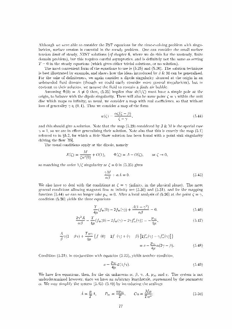
Although we were able to onsider the ZST equations for the time-evolving problem with singu-
larities, surfa e tension is essential in the steady problem. One an onsider the small surfa e
tension limit of steady, NZST solutions ( f hapter 6, where we do this for the unsteady, �nite
domain problem), but this requires areful asymptoti s, and is de�nitely not the same as setting
T = 0 in the steady equations (whi h gives either trivial solutions, or no solution).
The most onvenient form of the equations to use is (5.25) and (5.26). The solution te hnique
is best illustrated by example, and shows how the ideas introdu ed by J & M an be generalised.
For the sake of de�niteness, we again onsider a dipole singularity situated at the origin in an
unbounded uid domain (though we ould easily onsider more general singularities), but in
ontrast to their solution, we assume the uid to ontain a �nite air bubble.
Assuming �(0) = A 6= 0 then, (5.25) implies that �w(1=�) must have a simple pole at the
origin, to balan e with the dipole singularity. There will also be some point � = within the unit
dis whi h maps to in�nity; as usual, we onsider a map with real oeÆ ients, so that without
loss of generality 2 (0; 1). Thus we onsider a map of the form
w(�) =
��(� � �)
� �
; (5.44)
and this should give a solution. Note that the map (5.29) onsidered by J & M is the spe ial ase
= 1, so we are in e�e t generalising their solution. Note also that this is exa tly the map (5.1)
referred to in x5.2, for whi h a Hele-Shaw solution has been found with a point sink singularity
driving the ow [33℄.
The usual onditions apply at the dipole, namely
X (�) =
M
�w
0
(0)
+O(1); �(�) = A+O(�); as � ! 0;
so mat hing the order 1=� singularity at � = 0 in (5.25) gives
M
��
+ �A = 0: (5.45)
We also have to deal with the onditions at � = (in�nity, in the physi al plane). The most
general onditions allowing stagnant ow at in�nity are (5.30) and (5.31), and for the mapping
fun tion (5.44) we an no longer take p
1
= 0. After a lo al analysis of (5.26) at the point � = ,
ondition (5.30) yields the three equations
T
4�
(f
+
(0)� 2f
+
( )) +
A(1�
2
)
��
= 0; (5.46)
2
2
A
��
�
T
4�
(f
+
(0)� 2f
+
( )� 2 f
0
+
( )) = �
p
1
4�
; (5.47)
A
�
(1� � ) +
T�
4�
�
f
+
(0)� 2f
+
( ) + ( � �)
�
2f
0
+
( ) + f
00
+
( )
�
= �
p
1
4�
�(2 � �): (5.48)
Condition (5.31), in onjun tion with equation (5.25), yields another ondition,
=
p
1
4�
�w(1= ): (5.49)
We have �ve equations, then, for the six unknowns �, �, , A, p
1
and . The system is not
underdetermined however, sin e we have an arbitrary lengths ale, represented by the parameter
�. We may simplify the system (5.45){(5.49) by introdu ing the s alings
^
A =
�
T
A; P
1
=
�p
1
T
; Ca =
M�
T�
2
; (5.50)
77

here, Ca is a Capillary number for the ow (measuring the relative e�e ts of vis osity and surfa e
tension), and the quantity P
1
is a dimensionless line pressure. If we also rede�ne the fun tions
f
+
(�) by writing
F
+
(�) = �f
+
(�); (5.51)
then they are independent of the s aling parameter �. With these s alings, and eliminating
between (5.48) and (5.49), we obtain the system:
�
^
A
+ Ca = 0; (5.52)
F
+
(0)� 2F
+
( ) +
4
^
A
�
(1�
2
) = 0; (5.53)
4
^
A
�
(1 +
2
) + 2 F
0
+
( ) = �P
1
; (5.54)
P
1
4
�
2
� � + 1
(1�
2
)( � �)
= �
4
^
A
�
+
2
F
00
+
( ): (5.55)
We now have four equations for the four unknowns �, ,
^
A and P
1
. The Capillary number will
be spe i�ed as part of the problem. It is a simple matter to eliminate P
1
and
^
A, giving just two
equations to be solved for the mapping parameters � and ,
�
2
(F
+
(0)� 2F
+
( )) = 4Ca (1�
2
); (5.56)
4
�
2
� � + 1
(1�
2
)( � �)
(4(1 +
2
)Ca� 2�
2
F
0
+
( )) = 4Ca+ �
2
F
00
+
( ): (5.57)
These equations are still very diÆ ult though, sin e the fun tions F
+
( � ) depend nonlinearly on �
and , being de�ned through the expressions (3.8). A better notation emphasising this dependen e
would perhaps be F
+
( � ;�; ), but this is rather unwieldy.
Clearly, in the limit ! 1 we require P
1
= 0 for a balan e of terms in (5.55). In this limit,
equation (5.53) redu es to an identity, and what remains is equivalent to the problem solved by
J & M for the dipole in a half spa e.
The set of solution pairs (�; ) to (5.56) and (5.57) des ribe a set of equilibrium bubble shapes
whi h are solutions to the dipole-at-the-origin problem. Sin e we expe t that there are very many
su h solution pairs, a sensible s heme for �nding solutions to these equations (whi h will need to
be done numeri ally) is to spe ify the value of we wish to onsider, and, eliminating Ca between
equations (5.56) and (5.57), �nd the orresponding value(s) of � whi h satis�es the equations (the
relevant Capillary number will then follow from either of the above equations). Note that the
mapping fun tion (5.44) an also des ribe bounded uid domains if we allow > 1; the governing
equations in this ase will be di�erent however, sin e the singularities of equation (5.25) within
the unit dis then o ur at � = 0, � = 1= and have to be mat hed appropriately.
Any solution pairs (�; ) whi h are found must be he ked for univalen y, sin e only univalent
mapping fun tions give a eptable solutions. For unbounded uid regions, the univalen y domain
in (�; ) parameter spa e is the union of the two regions
1
�
< < 1 (� > 0; 2 (0; 1));
and
� < �
�
2 +
1
�
(� < 0; 2 (0; 1));
re all that we assumed 2 (0; 1) at the outset. In � > 0; < 0 we require � > 0; < 0 (respe tively)
to satisfy the normalisation ondition w
0
(0) > 0. Typi al free boundary shapes des ribed by this
78

map are shown in �gure 5.8; note that the extremal onformal maps orresponding to points (�; )
on the boundary of the univalen y domain in � > 0 des ribe uid regions in whi h the bubble
has ollapsed to a slit, whi h is a ir ular ar (the limiting ase of �gure 5.8 (b))|su h domains
will be obtained as solutions as we allow the Capillary number to be ome unbounded (the ZST
limit).
As another example, we may onsider the solution of J & M as being the limit of yet another
family of maps. In their solution the parameter p
1
was identi ally zero, be ause the map satis�ed
(5.32) near the point � = 1 (the preimage of in�nity). We may onsider more general maps
having p
1
identi ally zero, provided we hoose an appropriate form for them. We know that the
onditions (5.30), (5.31) are the most general giving stagnant ow at in�nity; we also know that
(5.25) must hold globally. Hen e if �(�) is to remain O(1) as � ! , with X (�) behaving as
spe i�ed by (5.31), the fun tion �w(1=�) must have a pole at � = ; that is to say, if w(�) has a
pole at � = within the unit dis , it must also have a orresponding pole at the inverse point,
(� = 1= , in the ase 2 R), outside the unit dis . We again onsider a dipole singularity at the
origin, so the fun tion �w(1=�) must have another simple pole at � = 0. Hen e a possible mapping
fun tion giving a (steady) solution has the form
w(�) = �
�
� + ��
�
1
� �
�
1� �
��
: (5.58)
We ould onsider more ompli ated options, but restri t ourselves to this simplest possibility
satisfying all the requirements, sin e the solution of J & M again emerges as a spe ial limiting
ase. Note that unlike the last example, this map annot des ribe bounded uid domains.
The solution pro edure is essentially the same as for the previous example, but the algebra is
a little easier. Mat hing the singularity at the dipole in (5.25) gives (with the s alings of (5.50))
^
A
�
1� �
�
+
1
��
+ Ca = 0:
For the ondition at in�nity, we need only ensure that �(�) has a �nite limit as � ! , sin e
for this parti ular hoi e of mapping fun tion the ondition on X (�) at in�nity will then follow
automati ally from (5.25). With the fun tions f
+
( � ) rede�ned as in (5.51) this is easily seen to
require
^
A(1�
2
)
1� � ( + 1= )
+
4
(F
+
(0)� 2F
+
( )) = 0;
and
^
A(1 +
2
)
1� � ( + 1= )
+
2
2
F
0
+
( ) = 0:
Eliminating
^
A between these three equations gives two equations for � and , whi h also ontain
the Capillary number,
Ca(1�
2
)
(1� � ( + 1= ))
2
=
4
(F
+
(0)� 2F
+
( )); (5.59)
Ca(1 +
2
)
(1� � ( + 1= ))
2
=
2
2
F
0
+
( ): (5.60)
Again, one may seek solution pairs (�; ) to these equations by postulating a parti ular value for
2 (0; 1), eliminating Ca between equations (5.59) and (5.60), and �nding the orresponding
value(s) of � whi h gives a solution (the orresponding Capillary number then follows from either
equation). Thus, the equation to be solved for �, with spe i�ed, is
1�
2
1 +
2
=
F
+
(0)� 2F
+
( )
2 F
0
+
( )
;
79
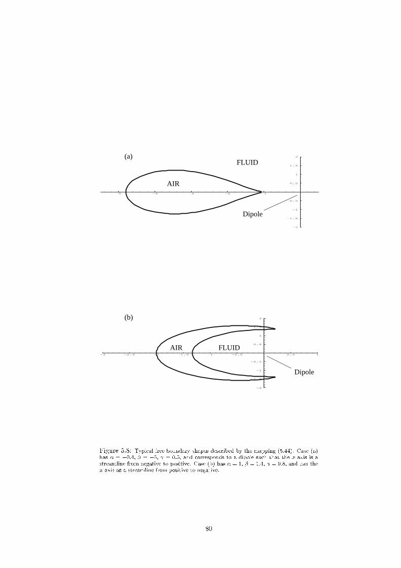
-5 -4 -3 -2 -1
-2
-1.5
-1
-0.5
0.5
1
1.5
2
-3 -2.5 -2 -1.5 -1 -0.5 0.5 1
-2
-1.5
-1
-0.5
0.5
1
1.5
2
(a)
(b)
AIR
AIR
FLUID
Dipole
FLUID
Dipole
Figure 5.8: Typi al free boundary shapes des ribed by the mapping (5.44). Case (a)
has � = �0:4; � = �5; = 0:5, and orresponds to a dipole su h that the x-axis is a
streamline from negative to positive. Case (b) has � = 1; � = 1:4; = 0:8, and has the
x-axis as a streamline from positive to negative.
80

-5 -4 -3 -2 -1 1
-10
-7.5
-5
-2.5
2.5
5
7.5
10
AIR
FLUID
Dipole
Figure 5.9: Typi al free boundary shape des ribed by the mapping (5.58). The parameter values used here are
� = �1; � = 3:5; = 0:65. The dipole at the origin is su h that the x-axis is a streamline from negative to positive.
81

the �-dependen e in this equation is entirely impli it in the fun tions F
+
( � ). Maps for solution
pairs (�; ) des ribe a family of equilibrium bubble shapes in a ow with a dipole singularity at
the origin. Only solution pairs (�; ) giving univalent maps are relevant; a typi al on�guration
is shown in �gure 5.9. For the map (5.58), the univalen y domain in (�; )-spa e is bounded by
the lines
� =
(1 + )
2
2
; = 1;
so the allowed parameter regime is
� >
(1 + )
2
2
; for 2 (0; 1):
There is no subset of the region � < 0, 2 (0; 1) whi h orresponds to a univalent map (we an
�nd univalent maps with � < 0, 2 (�1; 0), but these are equivalent to those already onsidered).
For points on the univalen y boundary, the bubble shape des ribed has a single usp in the free
boundary on the x-axis (at the point losest to the dipole). The situation shown in �gure 5.9
orresponds to a dipole su h that the x-axis is a streamline in the positive sense; for a dipole of
the opposite strength we have the \mirror image" situation (with � < 0, 2 (�1; 0)); there is no
analogue of �gure 5.8 (b).
5.6 Summary
This work of this hapter falls into two parts; the (ZST) Hele-Shaw results, and the Stokes ow
results. We began by reviewing the relevant literature for ea h, whi h is substantial, for both the
steady and time-dependent versions of the problems. Nevertheless, for the Stokes ow problem,
there is a gap in the literature: no solutions (obtainable by the omplex variable methods used in
this thesis) exist for time-dependent problems on unbounded ow domains, having a free boundary,
and driven by a singularity at some �nite point within the ow. Our task, whi h proved to be
far from trivial, was to �nd su h a solution by generalising the well-known (dipole driven) steady
solution of [52℄ to the time-dependent ase.
The Hele-Shaw version of this problem was solved in x5.3 and found to be a reasonably straight-
forward adaptation of a problem solved in [79℄, but with more interesting solution behaviour, sin e
the presen e of the dipole singularity (rather than a point sink) ne essitated a more ompli ated
mapping fun tion. In parti ular, the existen e of a \transient 5/2-power usp" solution was found
(see also [46℄, [50℄), where the free boundary formed a usp near the dipole, then immediately
smoothed, with a little air entering through the usp. The free boundary soon afterwards be ame
nonanalyti again, with the formation of two 3/2-power usps in the free boundary (�gure 5.7).
For the slow vis ous ow analogue, we saw that no physi ally-relevant solution to the problem
exists in the simplest ase with �(0) = 0; sin e the Goursat fun tion �(�) must be bounded at a
dipole singularity we were for ed to on lude that �(0) be �nite and nonzero. In this situation we
were able to solve for the singular part of the primitive of the S hwarz fun tion, and hen e dedu e
the distribution of singularities of �w(1=�) (the S hwarz fun tion itself) within the unit dis . The
main result was that a solution is only possible if the S hwarz fun tion has a time-dependent line
singularity within the unit dis . Due to the omplexity of the onformal map needed, the solution
was not ompleted.
We on luded the hapter by onsidering two (dipole driven) steady problems on unbounded
uid domains, both of whi h may be onsidered as generalising the solution of [52℄.
82

Chapter 6
Stokes ow with small surfa e
tension
We now abandon the simpli� ation we have hitherto assumed in most of our solutions, and move on
to onsider the time-dependent problem with positive surfa e tension, or the NZST problem. We
have mentioned already that remarkable analyti al progress has been made with this problem,
notably by Hopper [37, 38, 39℄, Ri hardson [82℄ and Howison & Ri hardson [49℄ (and see also
Tanveer & Vas on elos [96℄ in this ontext); Hopper uses somewhat more onvoluted methods
than ours to obtain his solutions. Two-dimensional problems that have been fully solved by the
methods of x3.3 or by Hopper's method in lude:
� the oales en e under surfa e tension of two (equal or unequal) ir ular ylinders of uid
[37, 82℄;
� the oales en e under surfa e tension of a ylinder and a half-spa e of uid [39℄;
� a lima� on-shaped uid domain evolving under the a tion of surfa e tension only [82℄;
� the evolution of domains des ribed by polynomial mapping fun tions of the form w(�) =
a(� � b�
n
=n) for any integer n > 2, evolving under the a tion of both surfa e tension and a
point sink at the origin [49℄;
� the evolution of bubbles in shear ow with surfa e tension in luded [96℄;
� the evolution of expanding/ ontra ting bubbles in quies ent ow with surfa e tension in-
luded [96℄.
The work that will most interest us here is that of Howison & Ri hardson [49℄, whi h we shall
hen eforth refer to as HR'95, sin e they in lude the e�e ts of both surfa e tension and a driving
me hanism. In addition, they introdu e a new on ept, whi h we shall all a weak solution to the
problem, and whi h we will be exploiting to solve a new problem.
6.1 Review of \weak" solutions
We begin by giving a short review of some of the work of HR'95, using their example to illustrate
the \weak solution" on ept. They onsider uid domains (t) having a single point sink of
strength Q at the origin, whi h are des ribed by the family of mapping fun tions
z = w(�; t) = a(� �
b
n
�
n
); j�j � 1; (6.1)
for a, b real and positive fun tions of time, and integers n � 2. The maps (6.1) are univalent on
the unit dis only if b < 1, with (n� 1) inward-pointing 3/2-power usps forming simultaneously
on � if b = 1.
83

Intermediate region
Outer problem
FLUID
AIR
FLUID
Inner region
Figure 6.1: The di�erent regions in the small surfa e tension \lima� on" problem, using
mat hed asymptoti s.
We an ir umvent some of the analysis of HR'95 if we use the results of x3.6, sin e we there
gave the \moment" evolution equations (3.34), and we have a polynomial map, for whi h the
\moments" were evaluated expli itly in equation (3.36). The form of the NZST equations (3.34)
makes it lear why a polynomial of the form above is so mu h easier than a general polynomial; it
means that we only need �nd f
+
(0), without worrying about any of the higher derivatives f
(r)
+
(0).
The only tri ky bit then is al ulating f
+
(0) using (3.8); on e this is done the evolution equations
dS
dt
=
d
dt
�
�a
2
�
1 +
b
2
n
��
= �Q; (6.2)
d
dt
(a
2
b) = �(n� 1)
T
��
abK(b); (6.3)
are immediate. Here, S(t) denotes the ross-se tional area of (t) and K(�) denotes the omplete
ellipti integral of the �rst kind (see [8℄, [30℄, or appendix B, for example).
The authors onsidered an (a; b) phase plane within the univalen y domain 0 � b � 1, a � 0,
a solution traje tory (a(t); b(t)) rea hing the boundary b = 1 being asso iated with formation of
3/2-power usps. Solution breakdown is inevitable when T = 0, with b(t
�
) = 1, a(t
�
) > 0 for
84

some positive \blow up" time t
�
(as expe ted, by the time-reversal argument of x1.4.2). However,
when T > 0 they found that one always has omplete extra tion of the uid from the domain,
with extra tion time t
E
= S(0)=Q su h that a(t
E
) = 0, b(t
E
) < 1. This naturally led them to
onsider the limiting ase T ! 0 where, ombining the previous two observations, usps form
in � at time t
�
< t
E
, and persist until time t
E
in a kind of \weak solution" s enario, where
a nonanalyti free boundary is permissible. This orresponds to a degenerate ase of equation
(6.3), where K(b) on the right-hand side is singular as b " 1 (in fa t the ellipti integral has the
asymptoti behaviour K(1� �) � �(1=2) log(�=8) as �! 0), but T ! 0 to ountera t this e�e t.
The net result is that b(t) is `pinned' at 1 for t > t
�
, whilst from (6.2), a(t) evolves a ording to
d
dt
�
a
2
�
1 +
1
n
��
= �
Q
�
; (6.4)
until t = t
E
, ZST theory holding for 0 < t < t
�
, of ourse. These weak
1
solutions are all of
similarity type for t
�
< t < t
E
, sin e only the s aling parameter a is hanging; the shape of the
free boundary remains the same throughout. So for instan e, the solution for n = 2 (whi h is
just the \lima� on" example of x3.4) will evolve as a shrinking ardioid for times t > t
�
in the
limit T ! 0. The authors investigate the velo ity �eld of the uid in the neighbourhood of the
\ usp", and �nd it to be �nite, being exa tly the velo ity of the free boundary itself (so there is
no entrainment of air into the usp). This an be easily he ked using the expression (C.1) in the
T ! 0 limit.
We note that if T is small and positive, the logarithmi nature of the singularity in K(b) as
b " 1 in (6.3) means that b(t) must be exponentially lose to 1 before surfa e tension e�e ts be ome
important, a fa t borne out in experiments, where `almost- usps', having radii of urvature whi h
are exponentially small in the Capillary number, an be observed; see for example [52℄.
2
In this small surfa e tension ase, 0 < T � 1, mat hed asymptoti s may also be used to solve
the problem, with three distin t r�egimes (�gure 6.1 illustrates this for the ase n = 2). The outer
solution will be the T ! 0 shrinking usped shape of HR'95. In the inner region, the free boundary
will be lo ally paraboli , a on�guration whi h was solved for in the NZST ase by Hopper [40℄
(the \Stokes ow Ivantsov" solution). The invarian e of Stokes ow under rigid-body motions
means that this solution an be a travelling wave of arbitrary speed. The apex urvature of the
parti ular parabola observed is a fun tion of the far-�eld ow imposed (whi h here is due to the
point sink). There will also be an intermediate region in whi h the inner and outer solutions are
mat hed. In this region, the geometry is su h that the free boundary may be linearised onto a slit,
and the Stokes equations solved on an unbounded domain with appropriate mat hing onditions.
Similar remarks apply to our solution of x6.2. We shall not onsider mat hed asymptoti s in
this thesis|see [67℄ for full details of the method applied to a similar Stokes ow problem (the
oales en e of two identi al ir ular ylinders).
6.2 The ubi polynomial map
We now onsider the ideas of HR'95 des ribed above, applied to a general ubi polynomial
mapping in the limit T ! 0. The ZST ase of the analogous Hele-Shaw problem was solved by
Huntingford in [50℄. As explained, we expe t the evolution of (t) to follow ZST theory until
the \blow up" time t
�
, at whi h point we relax the restri tion on � to permit solutions with
persistent usps in the free boundary. For ease of manipulation we hange notation slightly from
that above, writing
w(�; t) = a(t)
�
� +
b(t)
2
�
2
+
(t)
3
�
3
�
: (6.5)
1
These solutions are not \weak" in the true sense of the de�nition; we use the terminology be ause the solutions
are not lassi al. To avoid umbersome notation we now drop the inverted ommas when referring to them.
2
In this paper (whi h was dis ussed in detail in x5.4), the radius of urvature at the near- usp is found to be
proportional to exp(�32�Ca).
85

The s aling fa tor a may learly be taken to be real and positive for all time. By suitably rotating
the o-ordinates in the initial domain (0), the general ase with both b(0) and (0) omplex
may be redu ed to an initial map with just one omplex oeÆ ient. For simpli ity we shall
assume b(0); (0) 2 R, whi h will then ensure b(t) and (t) are real for t > 0; this is equivalent
to the assumption that (t) is symmetri about the x-axis. We return to the limitations of our
assumption in x6.2.1. For this ase, (3.34) and (3.36) yield
d
dt
�
a
2
�
1 +
b
2
2
+
2
3
��
= �
Q
�
; (6.6)
d
dt
�
a
2
b
�
1 +
2
3
��
= �
T
2�
f
+
(0)a
2
b
�
1 +
2
3
�
�
T
�
f
0
+
(0)
2
3
a
2
; (6.7)
d
dt
[a
2
℄ = �
T
�
f
+
(0)a
2
: (6.8)
With T = 0 these equations are valid until the time t
�
at whi h the map eases to be univalent.
As in [50℄ we must onsider the domain V in (b; )-spa e for whi h (6.5) is univalent
3
on j�j � 1,
and �nd the phase traje tories of the system (6.7), (6.8) within V . The determination of this
univalen y domain (in the more general ase of omplex oeÆ ients) is the subje t of [15℄. For
real oeÆ ients, V is symmetri about the -axis (so we lose nothing by restri ting attention to
the right-half plane), and is bounded in b > 0 by the lines
= 1; b = 1 + ; and
b
2
4
+ 4
�
3
�
1
2
�
2
= 1: (6.9)
The line b = 1 + orresponds to formation of a single 3/2-power usp on �, ex ept for the
isolated points (0;�1) (where we have two 3/2-power usps, symmetri ally pla ed about both
axes), and (8/5, 3/5) (where we have a single 5/2-power usp). The line = 1 orresponds to two
3/2-power usps on � (symmetri ally pla ed about both axes when b = 0), and the ellipti al
segment of �V (whi h extends from b = 8=5 to b = 4
p
2=3) orresponds to loss of univalen y by
the free boundary beginning to overlap itself. The domain V , together with the phase paths for
the T ! 0 solution, is shown in �gure 6.4. Figure 6.2 shows free boundary \blow-up" shapes for
various parameter values on �V .
Equations (6.7) and (6.8) give the ZST phase paths within V as the urves
b
�
1 +
2
3
�
= onst = k; (6.10)
for various k 2 R. In ontrast to the Hele-Shaw result of [50℄, we �nd no phase paths whi h
meet �V tangentially and then re-enter V ; all ZST solutions blow up with the phase path hitting
�V obliquely. A tangent phase path is asso iated with the instantaneous formation of a usp,
whi h immediately smooths (when the phase path re-enters V ), and the free boundary be omes
analyti again (the only known examples of su h behaviour for the Stokes ow [85℄ and Hele-Shaw
problems involve transient 5/2-power usps).
The ZST evolution is then fully determined, and we now onsider the e�e t of small positive
surfa e tension, as we approa h �V along a phase path. Using the de�nition (3.8), we are able to
�nd exa t expressions for f
+
(0) and f
0
+
(0) in terms of ellipti integrals. These exa t expressions are
ne essary if we wish to onsider the problem with O(1) surfa e tension, but not very illuminating
for the present dis ussion of the limit T ! 0; hen e we relegate the details to appendix B. The
main point to note is that they are singular only on the straight-line portions of �V (i.e. those
portions orresponding to blow-up via usp formation rather than by overlapping) and so only in
the neighbourhood of these lines will surfa e tension e�e ts be signi� ant, justifying our earlier
assumption that ZST theory is adequate for t < t
�
. To �nd the phase paths near �V , we ombine
3
Note, though, that we are a tually onsidering the proje tion of a \univalen y ylinder" in (a; b; ) spa e, onto
a = 1, with (6.6) providing the extra information about the variation of a with time.
86

-1.5 -1 -0.5 0.5 1 1.5
-1
-0.75
-0.5
-0.25
0.25
0.5
0.75
1
-1 -0.5 0.5 1 1.5 2
-1.5
-1
-0.5
0.5
1
1.5
-2 -1 1 2 3
-2
-1.5
-1
-0.5
0.5
1
1.5
2
-0.65 -0.55 -0.5 -0.45 -0.4
-0.04
-0.02
0.02
0.04
-1 1 2 3
-2
-1.5
-1
-0.5
0.5
1
1.5
2
-0.55 -0.5 -0.45 -0.4
-0.03
-0.02
-0.01
0.01
0.02
0.03
-1 1 2 3
-1.5
-1
-0.5
0.5
1
1.5
-1.5 -1 -0.5 0.5 1 1.5 2 2.5
-1.5
-1
-0.5
0.5
1
1.5
-2 -1.5 -1 -0.5 0.5 1 1.5 2
-1.5
-1
-0.5
0.5
1
1.5
(1) (2) (3a)
(3b)
(5) (6)
(4a) (4b)
(7)
AirFluid
AirFluid
Fluid Fluid Fluid
Fluid
Fluid Fluid Fluid
Figure 6.2: Free boundary shapes des ribed by the map (6.5) for various points (b; ) on the boundary �V
of the univalen y domain. The values used are: (b
1
;
1
) = (0; 1), (b
2
;
2
) = (1; 1), (b
3
;
3
) = (4
p
2=3; 1),
(b
4
;
4
) = (1:8; 0:8461), (b
5
;
5
) = (8=5; 3=5), (b
6
;
6
) = (1; 0), and (b
7
;
7
) = (1=5;�4=5). Pi tures (3b) and
(4b) are magni� ations of the nonunivalent region, showing how the free boundary begins to overlap itself; the
former ase is usped and self-overlapping, while the latter is smooth. The value a = 1 was used to generate ea h
pi ture, hen e the shapes do not have equal areas.
87

(6.7) and (6.8), writing a
2
= A, and a
2
b(1 + 2 =3) = B, to give
4
dB
dA
=
B
2A
+
2
3
f
0
+
(0)
f
+
(0)
; (6.11)
and hen e it is only the ratio of f
0
+
(0) to f
+
(0) whi h is important.
We need to onsider two separate ases, a ording as to whether the ZST solution breaks down
by rea hing = 1, or by rea hing b = 1 + (refer forward to �gure 6.4). Consider �rst the lass
of solutions for whi h " 1 within �V , along a ZST phase path. On e has rea hed a value lose
to 1, it is `trapped' near = 1 until either the solution blows up (with = 1 and attendant usp
formation, or with ' 1, b ' 4
p
2=3 on the ellipti al portion of �V , and self-overlapping of the
free boundary), or all uid is extra ted, sin e if de reased mu h below 1, ZST theory would
again take over, for ing it ba k up towards = 1 on a ZST phase path. It follows that only a and
b will be varying appre iably with time, and so A � a
2
, B � 5a
2
b=3. The results of appendix B
show that near = 1,
f
0
+
(0)
f
+
(0)
� �
b
2
� �
3B
10A
;
hen e (6.11) be omes
dB
dA
�
3B
10A
;
giving B = ( onst.)�A
3=10
, or, in terms of the mapping fun tion parameters,
b � ( onst.)� a
�7=5
; � 1: (6.12)
Knowing that ZST theory will hold until � 1, we may take t
�
(the ZST \blow up" time) to
be zero without loss of generality and pro eed from there, so that, in the limit T ! 0, (t) � 1
throughout the motion. Thus, from (6.6) and (6.12), the equations to be solved are
a
2
�
4
3
+
b
2
2
�
=
S(0)�Qt
�
= a
2
�
�
4
3
+
b
2
�
2
�
�
Qt
�
; (6.13)
and b = b
�
�
a
�
a
�
7=5
; (6.14)
where we use S(t) to denote the area of (t), and a
�
; b
�
denote the starting values of a and b
(
�
= 1, remember). The right-hand side of (6.13) is simply a linearly de reasing fun tion of time,
rea hing zero at \extra tion time" t
E
= S(0)=Q. Substituting from (6.14) in (6.13) gives
G(b)�G(b
�
) = �
6Qt
�a
2
�
b
10=7
�
; where G(b) := b
�10=7
(8 + 3b
2
): (6.15)
Now, G(b) is positive and monotone de reasing in b on the range of interest (namely 0 � b �
4
p
2=3), so (6.15) tells us that b must be monotone in reasing in t, from the starting value b
�
.
Hen e the phase path must follow the line = 1 in this dire tion, ending either at time t
E
, or
when it rea hes b = 4
p
2=3. Complete extra tion annot o ur in this r�egime, sin e (6.13) and
(6.14) give the area of the uid domain as
S(t) = �
4
3
a
2
+
b
2
�
a
14=5
�
2a
4=5
!
;
whi h is always positive. Hen e we dedu e that the phase path rea hes b = 4
p
2=3 before all the
uid has been extra ted, and the solution breaks down with � beginning to overlap itself (�gure
6.2 (3a) and (3b)).
4
Note that B and A are proportional to the 2nd and 3rd Stokes ow \moments" of the map (6.5), from the
de�nition (3.36).
88

We now onsider the ase of solutions approa hing the straight-line portion b = 1 + of �V
along a ZST phase path, observing, by the same argument as above, that a phase path will be
`trapped' near this line on e it is suÆ iently lose to it (�gure 6.4). We may thus eliminate either
b or in the ZST limit, and we hoose to work with b (so = b� 1). In this ase, A � a
2
(b� 1)
and B � a
2
b(2b+ 1)=3. The asymptoti evaluation of the ratio f
0
+
(0)=f
+
(0) as the line b = 1 +
is approa hed is performed in appendix B. This limit is found to be nonuniform on the range
b 2 (0; 8=5), being equal to �1 everywhere ex ept at the single point b = 0. Thus for b > 0 (6.11)
be omes
dB
dA
�
B
2A
�
2
3
;
whi h has solution
B = �
4A
3
+ �
p
jAj;
for some onstant �. We again take t
�
= 0 without loss of generality, and our initial onditions
must satisfy b
�
= 1 +
�
(where now 0 � b
�
� 8=5). In terms of a and b then, we have
a
jb� 1j
1=2
(2b
2
+ 5b� 4) =
a
�
jb
�
� 1j
1=2
(2b
2
�
+ 5b
�
� 4) � 3�;
holding together with the mass onservation equation (6.6) whi h, after some rearrangement, and
putting = b� 1 (sin e we remain on this part of the univalen y boundary), be omes
�
a
a
�
�
2
h(b)� h(b
�
) = �
6Qt
�a
2
�
;
for h(b) de�ned by
h(b) := 5b
2
� 4b+ 8 � 6
�
1 +
b
2
2
+
(b� 1)
2
3
�
:
Combining the previous two equations, eliminating the ratio a=a
�
between them, we �nally arrive
at an analogue of (6.15),
jb� 1j
h(b)
g(b)
2
� jb
�
� 1j
h(b
�
)
g(b
�
)
2
= �
6Qt
�a
2
�
jb
�
� 1j
g(b
�
)
2
; (6.16)
where g(b) := 2b
2
+ 5b� 4. Ignoring the ex eptional ases b
�
= 1, � = 0 for the moment (on our
range of interest, � = 0 o urs if and only if b
�
= b
= (�5+
p
57)=4), we see that the right-hand
side of (6.16) is a monotone de reasing fun tion of time, and so the left-hand side must be also,
i.e. F (b) := jb� 1jh(b)=g(b)
2
de reases with time. The area of the uid domain is given by
S(t) =
�a
2
�
h(b
�
)
6
F (b)
F (b
�
)
;
so omplete extra tion o urs if and only if F (b) falls to zero; this orresponds to extra tion time
t
E
= �a
2
�
h(b
�
)=(6Q). A plot of F (b) on (0; 8=5) is given in �gure 6.3 (b = 8=5 is the point at whi h
the form of �V hanges, the small ellipti al portion of �V for 8=5 < b < 4
p
2=3 orresponding to
blow up of solutions by overlapping of the free boundary). Important features to note are that:
� F (b) vanishes only at b = 1;
� F (b) has a singularity at b = b
, orresponding to a riti al point in the phase diagram;
� F (b) is monotone in reasing (to in�nity) on (0; b
), monotone de reasing (to zero) on (b
; 1),
and monotone in reasing on (1, 8/5);
89

0.2 0.4 0.6 0.8 10
0.5
1
1.5
2
2.5
3
1.1 1.2 1.3 1.4 1.5 1.60
0.02
0.04
0.06
0.08
0.1
0.12
0.14
Figure 6.3: The fun tion F (b) governing evolution on the part b = 1 + of �V . (Note the di�eren e in s ales
between the two plots.)
� F
0
(b) = 0 at b = 8=5, and only there, orresponding to the formation of the 5/2-power usp.
Hen e for b
�
2 (b
; 1) and b
�
2 (1; 8=5), the phase path will approa h the point b = 1, = 0, with
omplete extra tion o urring when we rea h this point, sin e we must have F (b) de reasing with
t. By ontrast, if b
�
2 (0; b
) we must have the phase path approa hing b = 0, = �1. Sin e
F (0) > 0, this point is rea hed before all the uid has been extra ted, but due to the symmetry
of the phase diagram about the -axis, we are for ed to stay at this point. For the moment we
ignore the ompli ations hinted at by the nonuniformity of the limit f
0
+
(0)=f
+
(0) at this point.
Re all now the omment in footnote (3), that we have a tually been onsidering the proje tion
of a univalen y ylinder by suppressing the parameter a. We are thus in one of the spe ial ases
onsidered in HR'95; the subsequent evolution will be of the `similarity' type dis ussed there,
with b � 0, � �1, and the parameter a hanging in a ordan e with the orresponding mass
onservation equation. The full phase diagram in the (b; )-plane is given in �gure 6.4, with phase
paths that are in some way `spe ial' represented by dashed lines. The bold arrows indi ate the
sense in whi h the phase paths `turn around' as they hit �V .
It is now apparent that the `ex eptional ases' b
�
= 1, b
�
= b
mentioned earlier are stable
and unstable (respe tively) riti al points in the phase diagram, and thus also represent possible
`similarity' solutions of the kind studied in HR'95, the dotted phase path = 0 being exa tly one of
those solutions. Note that for this spe ial solution, rea hing b = 1 no longer need be synonymous
with total extra tion, sin e the right-hand side of (6.16) is now identi ally zero; indeed, by the
analysis of HR'95 we do remain a �nite time at (1; 0) before extra tion is omplete. The points
(0;�1) and (0; 1) are also riti al points, stable (but see x6.2.1) and unstable respe tively, and
again, are members of the family of similarity solutions of HR'95. We may summarise our results
as follows:
� Phase paths whi h hit �V at (1; 0) or (0;�1) terminate there and represent stable similarity
solutions, sin e adja ent phase paths are also entering these points.
� Paths whi h hit �V at (0; 1) and (b
; 1�b
) terminate there and represent similarity solutions
whi h are unstable, sin e neighbouring paths are diverging.
� Paths for whi h
�
= 1, b
�
2 (0; 4
p
2=3) turn to the right and follow �V along = 1,
rea hing (4
p
2=3; 1) before extra tion is omplete, at whi h point the free boundary begins
to overlap itself. The present analysis then no longer applies, and the solution annot be
ontinued.
90

0 0.2 0.4 0.6 0.8 1 1.2 1.4 1.6 1.8 2−1
−0.8
−0.6
−0.4
−0.2
0
0.2
0.4
0.6
0.8
1
b
Blow-up
by overlapping
only on this urved
portion of �V
Two 3/2-power usps in �D along line = 1
5/2-power usp
Complete extra tion
Criti al point b
Two 3/2-power usps (symetri ally pla ed) at b = 0, = �1.
forms here
o urs here
One 3/2-power usp in �D along line b = 1 + (b 6= 0; 1; 8=5).
Figure 6.4: The univalen y diagram (restri ted to the right-half (b; )-plane) for the ubi polynomial mapping
fun tion. The shaded region orresponds to a nonunivalent map.
91

� Paths hitting the urved portion of �V likewise represent self-overlapping uid domains,
and annot be ontinued.
� Paths for whi h
�
= b
�
� 1, 1 < b
�
< 8=5 turn around and enter the point (1; 0); rea hing
this point is simultaneous with omplete extra tion.
� Ditto for b
< b
�
< 1.
� Paths for whi h
�
= b
�
� 1, 0 < b
�
< b
turn around and enter (0;�1), rea hing this point
before extra tion is omplete; subsequent evolution is of `similarity' type and is dis ussed in
HR'95.
In addition, an analysis of the velo ity �eld in the neighbourhood of the usp has been arried
out, using the expression (C.1) with T ! 0. The same result as in HR'95 was found (although
we do not give the analysis): the velo ity at the usp is exa tly the (�nite) velo ity of the free
boundary at that point, so there is no entrainment of air into the usp.
The 5/2-power usp is an interesting borderline ase, being the point of transition between
ZST solutions whi h break down via formation of a 3/2-power usp, and those whi h break down
via overlapping of the free boundary. This path must still turn around and enter (1; 0); however,
the fa t that F
0
(8=5) = 0 (�gure 6.3) implies that this path `only just makes it'. Geometri ally, the
5/2-power usp immediately be omes a 3/2-power usp, whi h then persists. The point (1; 0) on
�V orresponds to a ardioid, but sin e rea hing this point is simultaneous with total extra tion,
this on�guration is not a tually attained.
The existen e of the point b
is also interesting. As we move along �V from (1; 0) towards
(0;�1), �(t) evolves ontinuously from a ardioid (with a usp on the left-hand side), to a fully
symmetri shape having usps on both sides. As is does so, a `dimple' develops on the right-hand
side (see (6) and (7) in �gure 6.2), whi h be omes more pronoun ed, eventually turning into the
se ond usp at (0;�1). It is perhaps not surprising then that there is some riti al point beyond
whi h the `dimple' is too large to disappear, and the ultimate shape has to have two usps. If the
dimple is small enough (i.e. b
�
> b
), then the ultimate shape will have just one usp. For the
solutions with
�
= 1, however, the possible geometries are su h that the two- usp state is always
unstable, and ultimate overlapping of the free boundary has to o ur.
6.2.1 Complex oeÆ ients
Re all that, near the start of x6.2, we stated that the assumption of real oeÆ ients in the mapping
fun tion (6.5) was equivalent to assuming symmetry of (t) about the x-axis. The results obtained
seem to have a remarkably ri h stru ture nonetheless; however they are somewhat de eptive, as
onsideration of the ase with omplex oeÆ ients reveals.
A little thought about the on lusions of x6.2 throws up an apparent ontradi tion: the point
(0;�1) in (b; )-spa e is stated to be a stable equilibrium point, whilst the point (0; 1) is an unstable
equilibrium point. But the two on�gurations are a tually identi al, one being a rotation through
angle �=2 of the other. In fa t, the on lusions regarding the point (0;�1) were a little suspe t
anyway, sin e we knew the limit f
0
+
(0)=f
+
(0) to be nonuniform at this point, but the analysis
away from this point did indi ate that it should be a stable equilibrium.
In the pre eding analysis, we have been onsidering a single, two-dimensional ross-se tion
of what is a tually a four-dimensional univalen y domain V
4
in omplex (b; )-spa e. In fa t,
bearing in mind the omments of footnote (3), the full univalen y domain for the map (6.5) will
be a ylinder in �ve-dimensional spa e, but the dependen e on the s aling parameter a is of no
onsequen e. Determination of this domain is the subje t of Cowling & Royster's (hen eforth C
& R) paper [15℄. There, the authors note that the ross-se tion =fbg = 0 of V
4
is symmetri
about the planes <fbg = 0 and =f g = 0, and so it may be assumed without loss of generality
that =fbg = 0 and <fbg � 0 (sin e this will still generate all possible free boundary shapes, up
to rotations and re e tions). Writing = + i� and taking b 2 R
+
, their paper then determines
this three-dimensional ross-se tion V
�
of V
4
for whi h the map (6.5) is univalent on the unit dis ;
however this domain is not simple, and is given in an impli it form whi h is diÆ ult to use.
92

Before exploring the stru ture of this domain further, we onsider the hanges wrought in the
evolution equations for the oeÆ ients by allowing them to be omplex. We assume still that
a 2 R
+
, but now write b = � + i� and = + i�, for real �; �; ; �. The equations governing
the ZST problem are found from (3.32) and (3.36), and are
d
dt
�
a
2
�
1 +
jbj
2
2
+
j j
2
3
��
= �
Q
�
; (6.17)
a
2
�
b+
2 b
3
�
= onstant; (6.18)
a
2
= onstant. (6.19)
To obtain the phase paths in the four-dimensional (�; �; ; �)-spa e we must equate real and
imaginary parts in these equations. The �rst is wholly real already, and in any ase (as we have
observed for the real oeÆ ients ase) is unne essary for determination of the phase paths. The
four real equations resulting from (6.19) and (6.18) are
a
2
= k
1
; (6.20)
a
2
� = k
2
; (6.21)
a
2
�
� +
2
3
(� + ��)
�
= k
3
; (6.22)
a
2
�
�+
2
3
(��� � )
�
= k
4
; (6.23)
whi h, for various values of these four arbitrary onstants k
1
to k
4
, will give paths in (�; �; ; �)-
spa e (after elimination of a). We now re all the statement of C & R that it is suÆ ient to onsider
the situation � = 0, � > 0. Suppose we seek su h solutions to the above equations (6.20){(6.23).
The �rst two are un hanged, whilst the se ond two be ome
a
2
�
�
1 +
2
3
�
= k
3
; (6.24)
a
2
�� = k
4
: (6.25)
Equations (6.20) and (6.21) give
�
= onstant;
whilst (6.24) and (6.25) give
1
�
+
2
3�
= onstant;
whi h together imply that either both � and must be onstant, or else � = 0. Supposing the
�rst ase, with � 6= 0, then to satisfy the equations we need both a and � to be onstant also, in
whi h ase the mass onservation equation annot hold (ex ept in the trivial ase Q = 0). Hen e
we must have � = 0, showing that the only family of solutions for whi h b 2 R throughout the
evolution are those already found for whi h 2 R also.
The result of C & R essentially says that restri ting attention to V
�
yields all possible free
boundary shapes, the remainder of V
4
onsisting of rotations and re e tions of shapes whi h are
ontained within V
�
. For a map with onstant oeÆ ients it is then suÆ ient to onsider V
�
, sin e
any free boundary on�guration an be generated by some point within V
�
provided the axes
are suitably hosen. With time-dependent oeÆ ients, we may hoose axes su h that the initial
on�guration (0) is generated by a point of V
�
; however the above shows that only if � = 0 will
the on�guration for t > 0 also be generated by a point of V
�
. Solution traje tories for � 6= 0 will
migrate to regions of V
4
outside V
�
.
93

C & R's observation is therefore of limited use, sin e the only family of solution traje tories
lying wholly within the three-dimensional ross-se tion V
�
� V
4
is the family of real solutions
already studied|all other solution traje tories will simply interse t V
�
at a single point. The full
four-dimensional spa e V
4
will be horribly diÆ ult (if not impossible) to determine and study. We
onsider instead whether we might �nd a three-dimensional solution family for the ase in whi h
is real, but b is omplex. Setting � = 0 in equations (6.20){(6.23) gives
a
2
= k
1
; k
2
= 0;
a
2
�
�
1 +
2
3
�
= k
3
; a
2
�
�
1�
2
3
�
= k
4
;
sin e (6.21) has redu ed to an identity, we are able to eliminate a from these equations to �nd
phase traje tories in (�; �; )-spa e: these will be determined by the two equations
�
�
1 +
2
3
�
= onstant;
�
�
1�
2
3
�
= onstant:
To get an idea of this three-dimensional ross-se tion of V
4
, all it V
z
, we onsider simple two-
dimensional ross-se tions. The ross-se tion � = 0 is the ase already studied (the domain V
given by (6.9)). The ross-se tion � = 0 orresponds to maps of the form
w(�)
a
= � +
i�
2
�
2
+
3
�
3
:
Making the substitutions � = �i
^
�, = � and w(�) = �iw(
^
�) we �nd that
w(
^
�)
a
=
^
� +
^
�
2
^
�
2
+
3
^
�
3
;
so the interse tion of V
z
with this ross-se tion is exa tly the domain V , but inverted with respe t
to ; all it V
y
. Likewise, we will have a ZST solution family lying entirely within V
y
, with phase
paths exa tly as for the real oeÆ ients ase, but inverted with respe t to . The T ! 0 limit is
also inferred from the earlier analysis.
The other two-dimensional ross-se tion of V
z
we an look at is = 0. This is parti ularly
easy, the map now being
w(�)
a
= � +
(� + i�)
2
�
2
;
so that w
0
(�) = 0 only if � = �1=(� + i�), and the map is univalent on the dis
�
2
+ �
2
� 1:
A solution family again lies in this ross-se tion (whi h we all V
o
), with solution traje tories
whi h are straight lines
�
�
= onstant;
as an be seen from (6.22) and (6.23) with = 0 = �. All points on the univalen y boundary are
equivalent, in the sense that the free boundary shapes represented by the maps are just rotations
of the same ardioid. The T ! 0 limit of this solution family will be of the \similarity solution"
type, with initial lima� ons be oming ardioids (before all the uid has been extra ted) whi h then
persist in a self-similar fashion until extra tion is omplete.
The s hemati diagram 6.5 indi ates how the three-dimensional domain V
z
�ts together. Given
the equivalen e of the ross-se tions V and V
y
, we now see plainly the equivalen e of the points
94

-1
0
1
-0.5
-0.25
0
0.25
0.5-1
-0.5
0
0.5
1
-1
-0.5
0
0.5
1
-0.5-0.25
0
0.25
0.5
-1
0
1
-1
-0.5
0
0.5
1
-0.5-0.25
0
0.25
0.5
-1
0
1
-1
-0.5
0
0.5
1-1
-0.5
0
0.5
1
-0.5
-0.25
0
0.25
0.5
-1
-0.5
0
0.5
1
-1
0
1
-1
0
1
-1
-0.5
0
0.5
1
-1
0
1
V
y
V
z
�
�
V
V
o
Figure 6.5: The three-dimensional univalen y domain V
z
� V
4
, and its two-dimensional ross-se tions V , V
y
and
V
o
. The arrows on V
y
indi ate how the point fb = 0; = �1g destabilises ( f. �gure 6.4).
95

fb = 0; = 1g and fb = 0; = �1g, and the arrows in �gure 6.5 show how this on�guration
destabilises.
This is obviously not the full story, sin e we have onsidered only a limited subset V
z
of
V
4
, whi h happens to ontain a family of solutions of whi h the real oeÆ ients ase is a sub-
family. In fa t this sub-family appears twi e within V
z
, as we have seen (in V and in V
y
) so there
is onsiderable repetition even within this limited subset. V
z
does not ontain all possible free
boundary on�gurations. On the other hand, the ross-se tion V
�
(� = 0) of V
4
is a minimal set of
possible free boundary shapes if axes are hosen appropriately, but omplex-parameter solutions
do not lie wholly within this spa e. Evolution in time annot be determined by studying V
�
then,
unless the analysis is somehow modi�ed to allow the oordinates within the uid domain to rotate
suitably in time|we do not onsider this possibility.
In on lusion, it seems that a omprehensive study requires the determination of the full
domain V
4
, sin e we an say little more by onsidering three-dimensional ross-se tions. We have
at least resolved the apparent paradox of the real oeÆ ients ase, whi h appeared to show that
identi al on�gurations were at on e stable and unstable.
6.3 Summary
In this hapter our prin ipal on ern has been with the (time-dependent) NZST Stokes ow
problem, in the limiting ase that the small positive surfa e tension tends to zero. We began by
listing the more notable ontributions to the NZST problem, most of whi h assume an O(1) surfa e
tension parameter. Only HR'95 have previously onsidered the T ! 0 limit in su h problems (the
\weak solution" on ept), and their work is des ribed in x6.1. Clearly, it only makes sense to
do this when onsidering problems for whi h the ZST version undergoes �nite time blow-up (the
unstable su tion problem, re all the omments in x1.4.2). For su h problems the T ! 0 limit
is not the same as the ZST problem: in the latter, the usp formation in the free boundary is
terminal, with solution breakdown o urring, but for the former this is not so.
Following HR'95 we found a new weak solution for the su tion problem, with a ubi polyno-
mial mapping fun tion with real oeÆ ients, whi h we dis ussed at some length. Some of these
solutions were found to permit the extra tion of all the uid from the uid domain, while some
underwent a topologi al hange (self-overlapping), beyond whi h the solution ould not be on-
tinued. In ontrast to the ZST Hele-Shaw result of [50℄ (using the same mapping fun tion), there
is no ontinuable 5/2-power usp solution in the ZST ase.
5
The quadrati and ubi \similarity solution" families of HR'95 were seen to be a subset of
our new family. Our solutions were seen to be unsatisfa tory, however, in that two identi al
on�gurations are apparently both stable and unstable, a paradox whi h is a onsequen e of the
\real oeÆ ients" simpli� ation. Hen e, in x6.2.1, we investigated the \ omplex oeÆ ients" ase.
While a omplete solution was found to be too ompli ated analyti ally, we were able to resolve
the apparent ontradi tion, and arrive at an understanding of how our solution family �ts into
the mu h larger family of omplex ubi solutions. In parti ular, it would appear that the generi
\limiting on�guration" (as extra tion time is neared) for those solutions whi h do not undergo
a hange of topology, is the ardioid solution of HR'95, this being the only stable point of the
univalen y boundary.
It was also found (although we did not give the analysis) that the velo ity �eld at the usp is
�nite, and equal to the velo ity of the free boundary at that point, so that there is no entrainment
of air into the usp (see HR'95 for the analysis in the simpler ase onsidered there). Viewed as
a regularisation of the Stokes ow su tion problem, this may be ontrasted with the analogous
slit regularisation for the Hele-Shaw problem, whi h was mentioned in x1.4.1, and is dis ussed in
detail in hapter 7.
5
Su h ontinuable solutions an be found for the NZST Stokes ow problem, however; see [85℄.
96

Chapter 7
Cra k and Anti- ra k solutions to
the Hele-Shaw model
We re all the omments of x1.4.1 where we mentioned the theory of \ ra ks" and their ZST limit,
\slits", in the Hele-Shaw problem. In this hapter we shall give a brief overview of the theory of
ra ks and slits, and introdu e the new on ept of what we all anti ra ks, whi h although very
di�erent in behaviour to ra ks, are in some sense omplementary. We shall be onsidering the
small, positive surfa e tension problem throughout, so it might be expe ted that the ZST model
applies; however, we will see that the the nonzero surfa e tension is a ru ial part of the theory.
7.1 Overview of ra ks and slits
The ra k/slit theories were developed by several authors in a series of papers [36, 62, 33℄ between
1988 and 1994. The models are an attempt to regularise the ill-posed ZST Hele-Shaw su tion
problem, whi h is known to exhibit �nite-time blow-up via usp formation in all but very spe ial
ases. The ZST model has to be invalid as su h usped on�gurations are approa hed, be ause
the urvature � of the free boundary be omes very large at the forming usp. When � = O(1=T ),
where T is the (small) surfa e tension parameter, the boundary ondition p = 0 on � is no
longer a valid approximation to the a tual boundary ondition p = �T on �. Thus, surfa e
tension e�e ts be ome important as we near usp formation (the ZST blow-up time), but only
in the neighbourhood of the usp. This statement forms the basi premise of the models: they
are, in e�e t, a lo al regularisation, a ting only at isolated points of the boundary, whi h on
physi al grounds we expe t to be those points at whi h blow-up of the ZST problem o urs. For
de�niteness, we assume a point sink-driven ow.
In the ase of the ra k model [62℄, the proposal is that the subsequent morphology (for times
lose to the ZST blow up time) is that of a thin �nger of air (a ra k) whi h penetrates the uid
domain and propagates rapidly towards the sink. By \rapidly", we mean that the motion of
the rest of the free boundary is negligible ompared to the motion of the ra k, as long as this
ontinues. Asymptoti methods are employed to study the evolution, and the ra k geometry for
later times is determined as an analyti ontinuation of some assumed initial geometry. Slits are
ra ks of zero thi kness, but the slit model an be derived independently of the ra k model, as
we shall see.
Before presenting the theories, we mention some of the experimental and numeri al eviden e
supporting them. Kopf-Sill & Homsy [59℄, and Couder et al. [14℄ have observed narrow �ngers
(of thi kness approximately 1/10 the hannel width) propagating in Sa�man-Taylor experiments.
These an be observed only under very arefully monitored onditions; in [59℄ for instan e, the
plates of the Hele-Shaw ell had to be s rupulously lean. The �ngers destabilise via dendriti
instabilities along the sides of the �nger, whi h are on a mu h shorter lengths ale than the �nger
length itself, and are negle ted in the ra k theory to be des ribed.
97
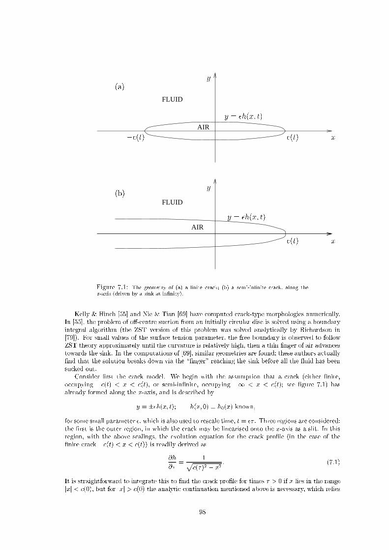
FLUID
AIR
AIR
FLUID
x
y
y = �h(x; t)
(t)� (t)
(t) x
y
y = �h(x; t)
(a)
(b)
Figure 7.1: The geometry of (a) a �nite ra k; (b) a semi-in�nite ra k, along the
x-axis (driven by a sink at in�nity).
Kelly & Hin h [55℄ and Nie & Tian [69℄ have omputed ra k-type morphologies numeri ally.
In [55℄, the problem of o�- entre su tion from an initially ir ular dis is solved using a boundary
integral algorithm (the ZST version of this problem was solved analyti ally by Ri hardson in
[79℄). For small values of the surfa e tension parameter, the free boundary is observed to follow
ZST theory approximately until the urvature is relatively high, then a thin �nger of air advan es
towards the sink. In the omputations of [69℄, similar geometries are found; these authors a tually
�nd that the solution breaks down via the \�nger" rea hing the sink before all the uid has been
su ked out.
Consider �rst the ra k model. We begin with the assumption that a ra k (either �nite,
o upying � (t) < x < (t), or semi-in�nite, o upying �1 < x < (t); see �gure 7.1) has
already formed along the x-axis, and is des ribed by
y = ��h(x; t); h(x; 0) � h
0
(x) known;
for some small parameter �, whi h is also used to res ale time, t = �� . Three regions are onsidered:
the �rst is the outer region, in whi h the ra k may be linearised onto the x-axis as a slit. In this
region, with the above s alings, the evolution equation for the ra k pro�le (in the ase of the
�nite ra k � (t) < x < (t)) is readily derived as
�h
��
=
1
p
(�)
2
� x
2
: (7.1)
It is straightforward to integrate this to �nd the ra k pro�le for times � > 0 if x lies in the range
jxj < (0), but for jxj > (0) the analyti ontinuation mentioned above is ne essary, whi h relies
98

on the assumption that
h( (�); �) = 0; � � 0:
(Here (�) is assumed monotone in reasing, whi h will be the ase if p
1
< 0, by the maximum
prin iple for Lapla e's equation.) With this assumption the inverse fun tion !(x), su h that
(!(x)) � x, may be de�ned, and expli it expressions for h(x; �) in both regions may be written
down,
h(x; �) = h
0
(x) +
Z
�
0
d�
0
p
(�
0
)
2
� x
2
; jxj < (0); (7.2)
h(x; �) =
Z
�
!(x)
d�
0
p
(�
0
)
2
� x
2
; jxj > (0): (7.3)
The latter equation here is the analyti ontinuation of the former. For the parti ular example of
a �nite ra k with an initially ellipti al pro�le, the shape of the ra k for later times turns out to
be a narrow ellipse [62℄.
There is also an inner region for the problem, in whi h the ra k is onsidered to have an O(1)
thi kness (by res aling y with �), and a tip region, in whi h both (x� (t)) and y are s aled with
�
2
, and surfa e tension e�e ts are important. In [36℄, onje tures are made whi h suggest that
the mat hing at the tip is only possible if � = T
1=3
. (In this paper, a balan e of terms in the tip
region is a hieved by s aling distan es with T
2=3
, time with T
�1=3
, and pressure variations with
T
1=3
; with these s alings the tip speed is O(T
�1=3
).)
The pro edure of analyti ontinuation of the initial geometry h
0
(x) is ill-posed, often leading
to the formation of singularities in the free boundary within �nite time, with subsequent blow-up
of the model. Examples of how this an o ur are given in [62℄, and spe ulation is made about
how the ra k might evolve through ertain types of singularities via tip-splitting.
The slit model (Hohlov et al. [33℄) on the other hand is well-posed, relying on onformal
mapping ideas whi h by now should be familiar to the reader. A slit is essentially a ra k of zero
thi kness, whi h again is postulated to propagate rapidly into the uid region. In this limiting ase,
\rapidly" will mean on a times ale su h that the rest of the free boundary is a tually stationary
whilst the slit is in motion. On physi al grounds, as for the ra k model, the expe tation is that
slits will grow from the ZST blow-up points of the free boundary; however, the slit model su�ers
from being seriously under-determined, permitting slits to propagate from arbitrary points of the
free boundary along arbitrary paths, and to bran h in any hosen way.
If a well-posed slit model exists, it ought to be realisable as the (ZST) limit of some ra k
model, and we will see that this is indeed the ase. The theoreti al framework for the model relies
on �rst rewriting the P-G equation (2.4) in the form
<
�
w
t
(�)
�w
0
(�)
�
=
�Q
2�jw
0
(�)j
2
on j�j = 1; (7.4)
(where the prime denotes �=��); as usual we take Q > 0 to represent a sink, sin e we are only
interested in the su tion problem. We have already mentioned that the model is under-determined;
however, physi al onsiderations suggest that we are interested in slit evolution for times t > t
�
(t
�
being the blow-up time for the ZST model), and from the point(s) on �(t
�
) at whi h the
usp forms. Time is thus res aled for t > t
�
with some small parameter �,
t� t
�
= ��; (7.5)
and the \slit mapping" is denoted by
W (�; �) = w(�; t
�
+ ��): (7.6)
For simpli ity, suppose a usp has formed at w(�1; t
�
) on the real negative axis, with the sink
lying at z = 0 (as in �gure 2.3, for example). To lowest order in �, (7.4) be omes
<
�
W
�
(�)
�W
0
(�)
�
= 0;
99

holding on j�j = 1, ex ept at � = �1, where the right-hand side is in fa t unbounded (so we expe t
something like a delta-fun tion there). In the absen e of other singularities on j�j = 1 Hohlov et
al. derive the appropriate form of (7.4) as
<
�
W
�
(�)
�W
0
(�)
�
= <
�
�a(�)
�
1� �
1 + �
��
;
for an arbitrary real, positive fun tion a(�). Res aling time again, and analyti ally ontinuing
this equation, they obtain a version of L�owner's di�erential equation for the mapping fun tion
W ,
W
�
(�)
�W
0
(�)
= �
�
1� �
1 + �
�
; (7.7)
holding globally. This is a linear, hyperboli p.d.e., with solution
W (�; �) = F (e
��
K(�));
for arbitrary fun tions F ( � ). Here K( � ) is the Koebe map of univalent fun tion theory (see [20℄),
de�ned by
K(�) =
�
(1� �)
2
;
whi h maps the unit dis onto the whole omplex plane, minus the slit (�1;�1=4℄ along the real
axis. The fun tion F ( � ) is determined from the initial data,
F (K(�)) =W (�; 0) � w(�; t
�
):
Hen e the \slit mapping" W (�; �) maps the unit dis onto the region (t
�
), minus the image
(under F ) of the slit [�1=4;�e
��
=4℄, so that the smooth portion of the free boundary remains
�xed at �(t
�
), whilst the point whi h was at w(�1; t
�
) has travelled into (t
�
) as far as the point
F (�e
��
=4). This is illustrated s hemati ally in �gure 7.2. By hoosing a suitable distribution
of delta-fun tions on the right-hand side of the P-G equation, more general versions of L�owner's
equation are obtained, and the above an be generalised to a model whi h allows slits to propagate
from arbitrary points of the free boundary, and in a spe i�ed manner (this is des ribed in [33℄),
hen e the indetermina y of the model referred to earlier. However, the justi� ation for writing
down (7.7) had a physi al basis, in that the singularity on the right-hand side was pla ed at
� = �1 be ause this is where the zero of w
0
(�; t
�
) o urred.
The link with the ra k model of [36, 62℄ an now be demonstrated. With time s aled as
in (7.5), we assume that the \slit" map W (�) of (7.6) represents only the �rst term in a simple
perturbation of the a tual mapping fun tion, in powers of � (the ra k thi kness), so that the free
boundary will be an O(�) distan e away from the slit. Thus, (7.6) is repla ed by
w(�; t) =W (�; �) + �W
1
(�; �) +O(�
2
):
We again substitute into (7.4); at lowest order we retrieve the slit problem, but at order � we get
<
�
�
�W
��
�W
1
��
+ �
�W
1
��
�W
��
�
= �
Q
2�
on j�j = 1: (7.8)
For the simple \paradigm" problem of a �nite ra k jxj < (�) driven by a sink at in�nity, with
sides y = ��h(x; �), the slit mapping is exa tly
W (�; �) =
2
(� + 1=�):
Substitution of this form for W into (7.8) with � = e
i�
and the normalisation Q = 2�, and noting
that at leading-order h(x; �) = =(W
1
(e
i�
)), and that x = (�) os �, leads eventually to
�h
��
=
1
p
(�)
2
� x
2
;
100

K
�
1
4
(0)
(�)
Time � > 0
Time � = 0
e
��
�
1
4
e
��
W (�; 0)K
�1
W (�; 0)
Figure 7.2: S hemati diagram showing how a general slit solution works.
101
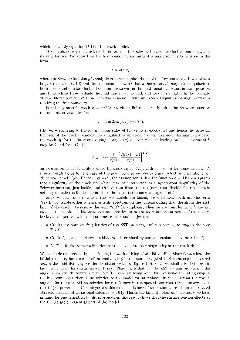
whi h is exa tly equation (7.1) of the ra k model.
We an also study the ra k model in terms of the S hwarz fun tion of the free boundary, and
its singularities. We know that the free boundary, assuming it is analyti , may be written in the
form
�z = g(z; t);
where the S hwarz fun tion g is analyti in some neighbourhood of the free boundary. It was shown
in x2.3 (equation (2.10) and the omments below it) that although g(z; t) may have singularities
both inside and outside the uid domain, those within the uid remain onstant in both position
and time, whilst those outside the uid may move around, and vary in strength. In the example
of x2.4, blow-up of the ZST problem was asso iated with an external square-root singularity of g
rea hing the free boundary.
For the symmetri ra k y = ��h(x; �), either �nite or semi-in�nite, the S hwarz fun tion
representation takes the form
�z = z � 2i�h(z; �) +O(�
2
);
(the +; � referring to the lower, upper sides of the ra k respe tively) and hen e the S hwarz
fun tion of the ra k boundary has singularities wherever h does. Consider the singularity near
the ra k tip for the �nite ra k lying along � (�) < x < (�). The leading-order behaviour of h
may be found from (7.3) as
h(x; �) �
1
(�)
�
2( (�) � x)
(�)
�
1=2
;
an expression whi h is easily veri�ed by he king in (7.1), with x = � Æ for some small Æ. A
similar result holds for the ase of the symmetri semi-in�nite ra k (whi h is a paraboli , or
\Ivantsov" ra k) [62℄. Hen e in general, the assumption is that the fun tion h will have a square-
root singularity at the ra k tip, whi h may be interpreted as a square-root singularity of the
S hwarz fun tion, just inside, and O(�) distant from, the tip (note that \inside the tip" here is
a tually outside the uid domain, sin e the ra k is the narrow �nger of air).
Sin e we have now seen how the two models are linked, we shall hen eforth use the term
\ ra k" to denote either a ra k or a slit solution, on the understanding that the slit is the ZST
limit of the ra k. We reserve the term \slit" for emphasis, when we are onsidering only the slit
model. It is helpful at this stage to summarise by listing the more important points of the theory,
for later omparison with the anti ra k results and onje tures.
� Cra ks are born at singularities of the ZST problem, and an propagate only in the ase
T > 0.
� Cra k tip speeds and ra k widths are determined by surfa e tension e�e ts near the tip.
� As T ! 0, the S hwarz fun tion g(z) has a square-root singularity at the ra k tip.
We on lude this se tion by mentioning the work of King et al. [56℄ on Hele-Shaw ows where the
initial geometry has a orner of internal angle � in the boundary (that is, � is the angle measured
within the uid domain; see the de�nition sket h of �gure 7.9), sin e we shall ite their results
later as eviden e for the anti ra k theory. They prove that, for the ZST su tion problem, if the
angle � lies stri tly between � and 2� (the ase 2� being some kind of inward-pointing usp in
the free boundary), there is no solution to the model for later times. In the ase that the orner
angle is 2� there is still no solution for t > 0, save in the spe ial ase that the boundary has a
(4n+ 1)=2-power usp (for integer n); this result is dedu ed from a similar result for the related
obsta le problem of variational al ulus [90, 64℄. This is the kind of \blow-up" geometry we have
in mind for regularisation by slit propagation; this result shows that the surfa e tension e�e ts at
the slit tip are an essential part of the model.
102

7.2 Introdu tion to Anti ra ks
Having reviewed the fundamental ideas behind ra ks and slits, we turn now to what we view as
the omplementary phenomenon of anti ra ks. These too will only arise in the ill-posed \su tion"
(and not in the \blowing") problem.
As the name suggests, in this ase, instead of having thin �ngers of air penetrating the uid
domain, we now have thin �ngers of uid whi h are \left behind" as the free boundary progresses
(refer forward to �gure 7.5). The two situations are very di�erent, despite the super� ial similar-
ities in the geometry. We know (by the maximum prin iple for harmoni fun tions) that, at least
for the ZST problem, the free boundary must always be moving down the pressure gradient (for
example, towards the sink, in a problem with a single point sink). Hen e, although �ngers of air
are able to propagate into the uid in a general su tion problem, �ngers of uid annot propagate
out but must, as we said, be \left behind". Thus the anti ra ks themselves are very stagnant (the
motion of the tip will be seen to be exponentially small for large time), although the rest of the
free boundary is able to propagate smoothly.
Su h stru tures are observable in Hele-Shaw experiments (Paterson [73℄ and Chen [11℄), and
large families of exa t solutions to the ZST model exist (Howison [45℄, Mineev-Weinstein & Pon e-
Dawson [66℄) whi h demonstrate anti ra k formation. In the experiments of [73℄ and [11℄ a less
vis ous uid is inje ted at a onstant rate into an expanse of more vis ous uid in a large Hele-
Shaw ell, and time-lapse photographs of the evolving interfa e are presented. The photographs
of both papers are remarkably similar, showing learly that long thin �ngers (the anti ra ks)
of the more vis ous uid are left behind as the free boundary advan es. Typi al results of the
experiments of [73℄ are reprodu ed in �gure 7.3. It is diÆ ult to see from these pi tures, but there
is a tenden y for the tips of the anti ra ks to be slightly bulbous for large times.
Paterson performs a linear stability analysis for the problem of an expanding ir ular \bubble"
of the less vis ous uid, whi h provides a surfa e tension dependent \sele tion me hanism" for
the �ngers, predi ting �rstly at what bubble radius they will start to form, and se ondly, whi h
of the unstable �nger wavelengths is fastest-growing when this radius is rea hed. We re onsider
this analysis in x7.6.
The radial �ngering solutions of [45℄, whi h are brie y onsidered in x7.3.3, an be made to
mimi losely the experimental results of [73℄ and [11℄ if the parameters in the onformal map are
hosen appropriately (�gure 7.3). Essentially, \ hoosing appropriately" means that the mapping
fun tion is hosen to give a judi ious distribution of singularities of the S hwarz fun tion within
the uid domain, whi h by the results of x2.3, must remain �xed within the ow domain, and
whi h the free boundary annot ross. In [45℄, a large lass of �ngering solutions in a hannel
geometry is also found, whi h are generalisations of the time-dependent Sa�man-Taylor �nger [88℄.
When wide �nger solutions of this type are onsidered as a periodi array, the anti ra ks be ome
apparent as the strips of uid separating these air �ngers, whi h were adja ent to the wall and
asymptoti ally stagnant in the hannel geometry. The solutions of [66℄, although non-periodi ,
are very similar to these solutions.
Remarkably similar geometries to the radial �ngering solutions (and experiments) have re ently
been omputed by Elliott & Gardiner [23℄, for the losely-related problem of the growth of a seed
of solid into a super ooled liquid (�gure 7.4). The authors use the phase �eld equations (with
suitably hosen parameters) to approximate the isotropi Stefan problem with Gibbs-Thomson
under ooling. The phase �eld equations are known to exhibit a wide range of possible behaviours
in di�erent parameter-group limits; in parti ular, various types of Stefan problem an be repre-
sented in this way, as well as the Hele-Shaw problem itself (see [9℄ for more dis ussion of these
matters).
In this hapter, we regard ra ks and anti ra ks as two di�erent possible regularisations of
the ill-posed \su tion" problem. A natural question to ask, then, is: What will determine whi h
instability is observed in a parti ular physi al situation? This is a key question, to whi h we return
in x7.9; although we are unable to give a ategori al answer, we make a onje ture (ba ked up by
analyti al, numeri al and experimental eviden e). Another question of interest on erns the e�e t
of surfa e tension on anti ra ks. We saw in x7.1 that the ra k/slit theory is ru ially dependent
103

Figure 7.3: Examples of the radial �ngering solutions of [45℄, together with a photograph of one of Paterson's
experiments [73℄.
104

Figure 7.4: Phase-�eld omputations of the \free boundary" (a tually a level set of
the phase parameter � o urring in the phase �eld model) for the growth of a seed of
solid into a super ooled liquid. This pi ture was kindly supplied by Dr A. R. Gardiner
[23℄.
105

on surfa e tension, sin e there is no solution to the ZST problem beyond the time at whi h it
blows up with formation of a 3/2-power usp [56℄ (whi h is the kind of situation we expe t to
be regularised by ra k formation). For the ase of anti ra ks, however, there exist large lasses
of solutions to the ZST problem whi h exist for all time, with analyti free boundaries. These
boundary urves should not be very di�erent to those for the orresponding small positive surfa e
tension problem, then|although surfa e tension must be the sele tion me hanism determining
whi h solution is observed. We also remark that the tenden y of the anti ra k tips to be ome
slightly bulbous for large times observed in [73℄ and [11℄ must be attributable to surfa e tension
e�e ts, sin e the tip is the most highly urved part of the free boundary in a narrow anti ra k.
7.3 Exa t ZST anti ra k solutions
Before making any more general omments, we present some exa t ZST solutions to the Hele-
Shaw problem whi h exhibit anti ra k formation. It is useful to do this, �rstly be ause it makes
lear what the mathemati al des ription of an anti ra k is, and se ondly, be ause by the above
omments regarding the small surfa e tension problem, we expe t su h solutions to be able to
provide a good des ription of the a tual behaviour observed. We will see, however, that the
ZST problem is underdetermined, having solutions whi h allow a more or less arbitrary array of
anti ra ks to be generated by suitable hoi e of the parameters in the onformal maps.
7.3.1 The \generi " anti ra k
We �rst present what we onsider to be the \generi " (and ertainly the simplest) Hele-Shaw
anti ra k solution, sin e it aptures all the essentials of the behaviour. It is a solution on a semi-
in�nite uid domain, driven by a onstant negative pressure gradient at in�nity, and is most easily
obtained by use of a onformal map from the right-half plane onto the uid domain. The map we
onsider is very simple,
w(�; t) = � + Ut+ � log(a(t) + �) <(�) � 0; (7.9)
where U and � are positive onstant parameters, and a(t) is a fun tion of time (assumed real,
without loss of generality). This map is easily seen to be a solution of the problem, for arbitrary
�, provided a satis�es the ondition
a+ Ut+ � log a = onst. = a
0
+ � log a
0
; (7.10)
where a
0
= a(0). This may be seen either by using the P-G equation (2.6), or by the results
of x2.3 (that those singularities of the S hwarz fun tion within the physi al domain must remain
�xed), noting that for a map from the right-half plane onto the uid domain, the S hwarz fun tion
is given by
g(z(�)) � �w(��): (7.11)
Equation (7.10) is not expli itly solvable for a(t), but the large-time behaviour, when the anti ra k
is well-developed, is easy to obtain. The only possible large-time balan e is a! 0 as t!1, with
the onstant � ne essarily positive. (If � < 0 a solution for a(t) must ease to exist within �nite
time.) Sin e here we are only interested in the large-time behaviour, we assume initial onditions
su h that the right-hand side of equation (7.10) vanishes; the asymptoti behaviour of a(t) is then
a(t) � exp(�Ut=�): (7.12)
The anti ra k tip is at
z
tip
= w(0)
= Ut+ � log a
= �a; (7.13)
106

the last equality following from (7.10) with zero right-hand side. Hen e with the asymptoti be-
haviour of (7.12), the anti ra k tip approa hes exponentially lose to the origin, but never a tually
rea hes it. This asymptoti stagnation of the tip is asso iated with a logarithmi singularity of
the S hwarz fun tion (given by (7.11)) at the point
z = w(a) = Ut+ a+ � log(2a)
= � log 2;
whi h the free boundary annot ross while the solution exists. The free boundary itself is given
by the image of the imaginary �-axis, � = i�. Taking real and imaginary parts in x+ iy = w(i�)
gives
x = Ut+
�
2
log(a
2
+ �
2
) � Ut+
�
2
log(�
2
+ exp(�2Ut=�));
y = � + � tan
�1
(�=a) � � + � tan
�1
(� exp(Ut=�)):
There are three distin t parts to the free boundary, orresponding to di�erent r�egimes for �. The
anti ra k tip is des ribed by j�j � exp(�Ut=�) � 1, or equivalently, j�j � a, so that a ording
to the above expressions,
x � 0; y � � tan
�1
(� exp(Ut=�))
� �� exp(Ut=�);
(although a better approximation for x is given by (7.13) and (7.12)). For a narrow anti ra k,
�� 1, and if we res ale x = �X , y = �Y , then in the tip region,
2X � log(1 + �
2
=a
2
); Y � tan
�1
(�=a);
and the general equation of the anti ra k tip is
Y = os
�1
(e
�X
):
The anti ra k sides are given by exp(�Ut=�)� j�j � ��=2, where
x � Ut+ � log j�j; y � �
��
2
:
The advan ing free boundary is given by j�j � ��=2, and for � in this range,
x � Ut+ � log jyj:
Intermediate values of � represent the smooth transition between these three regions; in parti ular,
we refer to the transition between the anti ra k sides and the advan ing free boundary as the
anti ra k root. A typi al large-time free boundary is shown in �gure 7.5. All su h free boundaries
are of self-similar form in any ase, there being only one free parameter in this solution (�=U , the
ratio of the anti ra k width to the uniform pressure gradient). Away from the tip, the rest of the
anti ra k annot \feel" its presen e, and the solution is essentially a travelling wave,
z = w(�) = � + Ut+ � log �; (7.14)
with an in�nitely long anti ra k of width ��.
The pressure �eld within the anti ra k is given by (2.1) and (2.5) as
p = �<(�):
Near the tip,
z � Ut+ � log(a+ �);
so with a given approximately by (7.12), the pressure �eld in the tip region is approximately
p � exp(�Ut=�)(e
z=�
� 1):
107

0.5 1 1.5 2
-4
-2
2
4
FLUID
AIR
t = t
1
t = t
2
t = t
3
y
x
Figure 7.5: A typi al \generi anti ra k" solution. The free boundary is shown for times t = t
1
; t
2
; t
3
, with
t
3
> t
2
> t
1
.
108

7.3.2 Solutions with many anti ra ks
Having seen how the solution for a single anti ra k works, it is a straightforward matter to gener-
alise to an arbitrary array of parallel anti ra ks, by suitable hoi e of the logarithmi singularities
in the mapping fun tion w(�). The solutions of this se tion were also given in [66℄ in the ontext of
general Lapla ian pattern formation (whi h of ourse in ludes the ZST Hele-Shaw problem), and
are losely related to the \ hannel geometry" solutions of [45℄ and [88℄, although the derivation
as given here was independent of this work.
The obvious form of mapping fun tion to try is
w(�) = � + Ut+
N
X
r=1
�
r
log(a
r
(t) + �); (7.15)
where all the �
r
are assumed to be real positive onstants, and the a
r
(t) fun tions of time with
positive real parts. This will give a solution of the P-G equation (2.6) provided the singularities
of the S hwarz fun tion (7.11) remain �xed in the physi al region, that is, provided the following
onditions hold:
a
n
(t) + Ut+
N
X
r=1
�
r
log(a
r
(t) + a
n
(t)) = k
n
; n = 1; : : : ; N; (7.16)
for N omplex onstants k
n
. The parameters �
n
represent the anti ra k widths (for large times,
when the anti ra ks are well-developed), and (�U) is the pressure gradient at in�nity. As with
the generi solution, U may be s aled out of the problem by dividing ea h of the �
n
by U . The
large-time behaviour of these solutions requires a little more are than the previous example,
sin e we are now dealing with omplex quantities. Writing a
n
= p
n
+ iq
n
and k
n
= �
n
+ i�
n
the
equations (7.16) be ome:
p
n
+
N
X
r=1
�
r
2
log[(p
n
+ p
r
)
2
+ (q
n
� q
r
)
2
℄ = �
n
� Ut; (7.17)
q
n
+
N
X
r=1
�
r
tan
�1
�
q
n
� q
r
p
n
+ p
r
�
= �
n
: (7.18)
A large-time balan e in (7.17) is only possible if ea h of the fun tions p
n
(t) is de aying expo-
nentially with time; the q
n
(t) will remain O(1). If we assume that q
n
6= q
m
for n 6= m then the
asymptoti behaviour of (7.17) will be
p
n
(t) �
1
2
exp
�
�
n
� Ut
�
n
�
;
whilst that of (7.18) will be
q
n
(1) = �
n
+
�
2
X
r 6=n
�
r
sgn(q
r
(1)� q
n
(1)):
If we assume the ordering is hosen su h that q
1
(0) < q
2
(0) < : : : < q
N
(0) (whi h will then persist
for later times), we have
q
n
(1) = �
n
+
�
2
X
r>n
�
r
�
�
2
X
r<n
�
r
; (7.19)
hen e the q
n
approa h known, onstant values as t!1.
This solution exists globally in time, with the parameter restri tions we have imposed. It
des ribes an array of N parallel anti ra ks, the n'th one having its tip at the point
z
n
= w(�iq
n
);
109

0.5 1 1.5 2 2.5 3
-4
-2
2
4
FLUID
AIR
Figure 7.6: A typi al solution generated by (7.15), showing 4 well-developed anti ra ks. Here, ��
i
=
0:5; 1; 0:8; 0:4; for i = 1; 2; 3; 4; respe tively; �
i
= �3; �2; 0:5; 1:5, and �
i
= 0:5 for ea h i.
su h that the orresponding logarithmi singularity of the S hwarz fun tion lies (�xed) within the
�nger tip, preventing the free boundary progressing beyond this point. Asymptoti ally then, the
anti ra k tips are �xed at the points
x
n
(1) � �
n
� �
n
log 2 +
X
r 6=n
�
r
log jq
r
(1)� q
n
(1)j; (7.20)
with the q
k
(1) given by (7.19), and
y
n
(1) � �q
n
(1) +
�
2
X
r>n
�
r
�
�
2
X
r<n
�
r
= ��
n
: (7.21)
The width of the n'th anti ra k is �
n
�. This impli itly assumes that the distan e between
adja ent anti ra k tips, j�
n+1
��
n
j, is greater than the sum of the two anti ra k half-thi knesses,
�(�
n
+ �
n+1
)=2, so that the anti ra ks are all distin t, although this is not ne essary for the
validity of the solution. All that we require is that the �
n
be real and positive, and that the
110
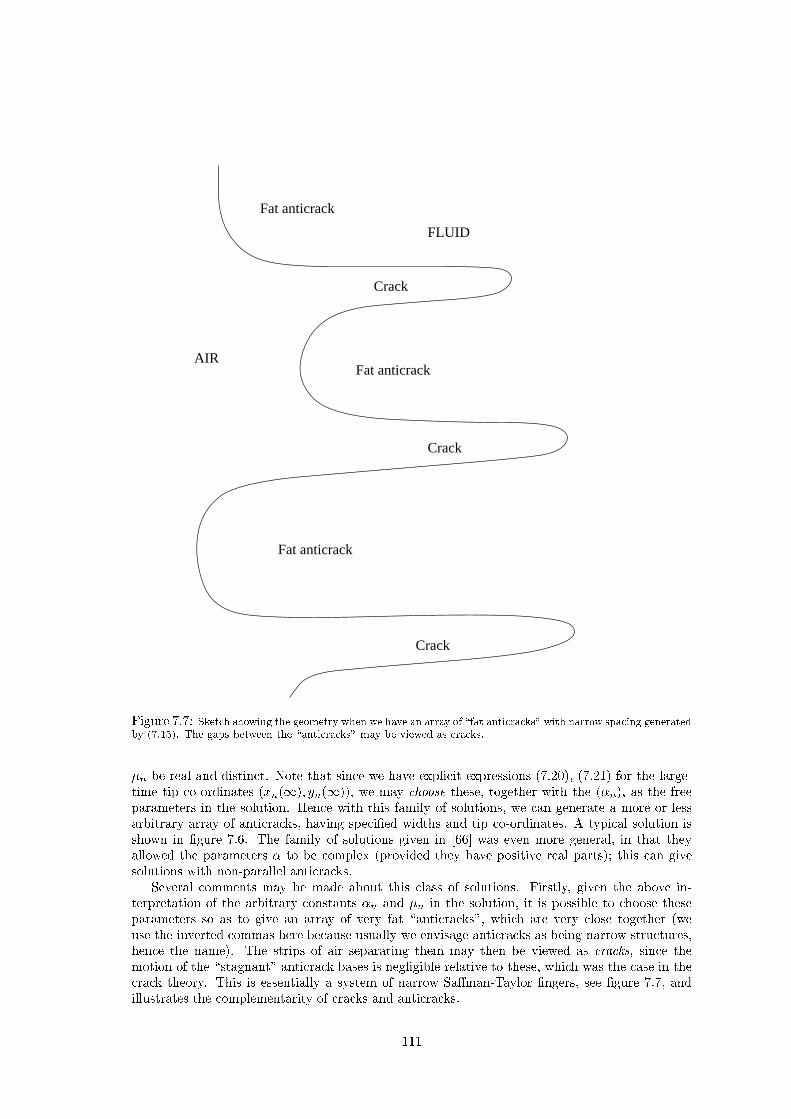
Fat anticrack
Fat anticrack
Fat anticrack
Crack
Crack
Crack
AIR
FLUID
Figure 7.7: Sket h showing the geometry when we have an array of \fat anti ra ks" with narrow spa ing generated
by (7.15). The gaps between the \anti ra ks" may be viewed as ra ks.
�
n
be real and distin t. Note that sin e we have expli it expressions (7.20), (7.21) for the large-
time tip o-ordinates (x
n
(1); y
n
(1)), we may hoose these, together with the (�
n
), as the free
parameters in the solution. Hen e with this family of solutions, we an generate a more or less
arbitrary array of anti ra ks, having spe i�ed widths and tip o-ordinates. A typi al solution is
shown in �gure 7.6. The family of solutions given in [66℄ was even more general, in that they
allowed the parameters � to be omplex (provided they have positive real parts); this an give
solutions with non-parallel anti ra ks.
Several omments may be made about this lass of solutions. Firstly, given the above in-
terpretation of the arbitrary onstants �
n
and �
n
in the solution, it is possible to hoose these
parameters so as to give an array of very fat \anti ra ks", whi h are very lose together (we
use the inverted ommas here be ause usually we envisage anti ra ks as being narrow stru tures,
hen e the name). The strips of air separating them may then be viewed as ra ks, sin e the
motion of the \stagnant" anti ra k bases is negligible relative to these, whi h was the ase in the
ra k theory. This is essentially a system of narrow Sa�man-Taylor �ngers, see �gure 7.7, and
illustrates the omplementarity of ra ks and anti ra ks.
111
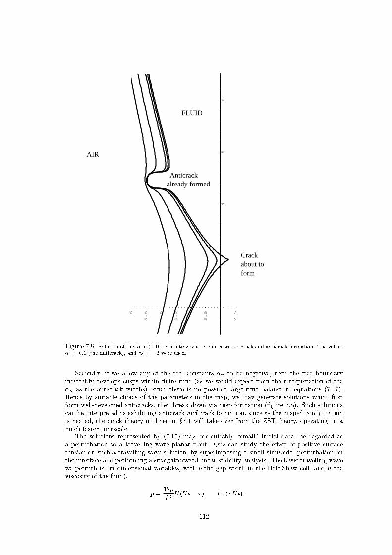
34
56
2.5
3.54
4.55
5.56
Anticrackalready formed
Crackabout toform
AIR
FLUID
Figure 7.8: Solution of the form (7.15) exhibiting what we interpret as ra k and anti ra k formation. The values
�
1
= 0:1 (the anti ra k), and �
2
= �3 were used.
Se ondly, if we allow any of the real onstants �
n
to be negative, then the free boundary
inevitably develops usps within �nite time (as we would expe t from the interpretation of the
�
n
as the anti ra k widths), sin e there is no possible large-time balan e in equations (7.17).
Hen e by suitable hoi e of the parameters in the map, we may generate solutions whi h �rst
form well-developed anti ra ks, then break down via usp formation (�gure 7.8). Su h solutions
an be interpreted as exhibiting anti ra k and ra k formation, sin e as the usped on�guration
is neared, the ra k theory outlined in x7.1 will take over from the ZST theory, operating on a
mu h faster times ale.
The solutions represented by (7.15) may, for suitably \small" initial data, be regarded as
a perturbation to a travelling wave planar front. One an study the e�e t of positive surfa e
tension on su h a travelling wave solution, by superimposing a small sinusoidal perturbation on
the interfa e and performing a straightforward linear stability analysis. The basi travelling wave
we perturb is (in dimensional variables, with b the gap width in the Hele-Shaw ell, and � the
vis osity of the uid),
p =
12�
b
2
U(Ut� x) (x > Ut);
112

where x = Ut is the free boundary. Perturbing the free boundary to
x = Ut+ �e
�t
sin
�
n�y
L
�
+O(�
2
);
we �nd the dispersion relation
� =
jnj�
L
�
U �
Tn
2
�
2
b
2
12�L
2
�
:
Here, T is the usual surfa e tension parameter, whi h when positive is seen to have the e�e t of
stabilising shorter wavelengths. Assuming walls at y = �L=2, there is a riti al (minimum) speed
for a perturbation to be maintained,
U
�
=
T�
2
b
2
12�L
2
;
whi h will typi ally be mu h less than unity, and hen e usually ex eeded. The fastest-growing
wavenumber is the n = 1 mode, so a ording to this analysis, if we have a hannel of width L
(not small), and hannel length mu h greater than L, an initially at interfa e might be expe ted
to evolve to a single dominant �nger (although this would rapidly take us beyond the realm of
the linear theory)|the Sa�man-Taylor experiment.
7.3.3 Howison's radial \anti ra k" solutions
For ompleteness, and also be ause of the remarkable similarity with the experimental pi tures of
[73℄ and [11℄, and the numeri al simulations of [23℄, we present the family of solutions found by
Howison [45℄. These solutions di�er from those above, being in a radial geometry, although the
essential anti ra k behaviour is the same.
We map from the unit dis onto the uid domain, whi h is here the exterior of some �nite
bubble. The mapping fun tion used is
w(�) =
a(t)
�
+ �
1
N
X
k=1
$
�k
log(
1
(t)$
k
� �)
+ �
2
N
X
k=1
$
�k�1=2
log(
2
(t)$
k+1=2
� �); (7.22)
for a,
1
,
2
real fun tions of time, with a > 0,
1
> 1,
2
> 1; the �
i
are positive onstants to be
hosen (analogous to the �
i
in the solution (7.15), in that ��
i
turns out to be the anti ra k width),
and $ is an N 'th root of unity (so $
N
= 1). More ompli ated maps, allowing asymmetri arrays
of �ngers to be generated, an be dealt with, but (7.22) is the ase onsidered in detail in [45℄.
The motion is assumed to be driven by a sink Q at in�nity. The fa t that the singularities of
the S hwarz fun tion must remain �xed in the physi al plane yields two invariants of the motion,
a
i
+ �
i
N
X
k=1
$
�k
log(
2
i
$
k
� 1) + �
j
N
X
k=1
$
�k�1=2
log(
i
j
$
k+1=2
� 1) = K
i
;
holding for i = 1, j = 2, and also for j = 1, i = 2, for some real onstants K
1
, K
2
. The third and
�nal equation governing the evolution is the ondition that the rate of hange of the bubble area
should be equal to Q,
a
2
�Na(�
1
1
+ �
2
2
) =
Qt
�
+K
0
;
for some real onstant K
0
. These equations ould also have been derived by dire t substitution
of (7.22) into the P-G equation (2.4), although this is mu h more tedious.
113

If the initial values
1
(0) and
2
(0) are large, then the initial domain will be nearly ir ular
(as may be seen from w(�; 0)). In any event, provided their initial values are greater than one,
both
1
and
2
will de rease monotoni ally to unity as t ! 1, and the bubble will leave behind
2N �ngers of uid, alternate �ngers having widths ��
1
and ��
2
. A typi al solution is shown in
�gure 7.3; we refer to [45℄ for the remaining details of the solution.
7.4 The S hwarz fun tion of an anti ra k
The solutions obtained so far indi ate that a general ZST anti ra k has a logarithmi singularity of
the S hwarz fun tion just inside the tip, whi h is �xed, and whi h the free boundary annot rea h
in �nite time ( ontrast this with the square-root singularity just outside the tip, for a ra k). We
have already seen how this works for the logarithmi singularity, but it is also easy to demonstrate
that the free boundary annot rea h a more general internal singularity, su h as g(z) � �(�� z)
m
for some onstants �, �, and m > 0.
1
We note, however, that although we onje ture this
logarithmi singularity to be generi for the ZST anti ra k, it annot be a singularity in the
NZST problem (even if we allow it to move), as may be seen from (2.11). Internal singularities
of the S hwarz fun tion will not now remain �xed in spa e (save those whi h oin ide with the
driving singularity) and must move in su h a way as to an el the singularity on the right-hand
side of (2.11). Motivated by a link between (2.11) and the well-known \Harry-Dym" equation, it
was onje tured in [48℄ that the anoni al moving singularity in the NZST problem is of the form
g(z) �
�(t)
(z � z
0
(t))
1=3
as z ! z
0
(t),
for some �(t), z
0
(t). It is easy to show that the oeÆ ients in this leading-order singularity, whi h
is of ourse mu h larger than log(z � z
0
) as z ! z
0
, satisfy
_z
0
=
4T
p
3�
3
:
We know that in the ZST limit we need _z
0
= 0, and we also expe t � = 0 for the generi anti ra k,
so dependen e like � � T
k
for 0 < k < 2=3 would do, for instan e. If our generi ZST anti ra k
is a sensible T ! 0 limit of some NZST anti ra k solution, and if the onje ture of [48℄ about
the anoni al NZST singularity is orre t, then there must be a se ondary logarithmi singularity,
whi h an persist as T ! 0, and whi h will dominate in this limit.
It is still the ase that the free boundary annot ross internal singularities of g(z) while the
solution exists. Given the photographi eviden e of [73, 11℄, and the ex ellent agreement with the
ZST solutions of [45℄, one therefore expe ts very little variation in z
0
(t) for large time. Further
progress with the NZST problem is diÆ ult, and we do not pursue it.
7.5 Results from formal asymptoti s
Having set the s ene by presenting some exa t ZST anti ra k solutions, we now digress a little
to onsider some results due to King et al. [56℄, whi h rely on formal asymptoti s in the neigh-
bourhood of singular points of the ow. We mentioned this work in x7.1, iting the result that in
the ill-posed ZST su tion problem, there exists no solution to the problem for t > 0 if the initial
free boundary �(0) ontains a orner of internal angle � 2 (�; 2�). In fa t, mu h more general
results than this are obtained, whi h we summarise below.
Consider the ZST su tion problem, where the initial domain (0) is nonanalyti , having a
orner of internal angle � in �(0) at x = 0 (�gure 7.9). Then:
1
Solutions to the ZST su tion problem an be onstru ted in whi h the free boundary rea hes a singularity
of the S hwarz fun tion within �nite time, but su h solutions are the time-reversals of blowing problems with
nonanalyti initial data (see for instan e [32℄), and therefore \pathologi al" examples.
114

FLUID
AIR Suction
x
y
0
�
Figure 7.9: The lo al geometry with a orner of internal angle � in the uid.
� If 0 < � � �=2, a solution an exist for t > 0; if it does, the boundary �(t) ontinues to
have a orner of angle � at x = 0.
� For �=2 < � < �, a solution an exist for t > 0; if it does, then for t > 0 the orner angle
swit hes instantaneously to (� � �).
� For � = �, if �(0) is analyti at x = 0 then the free boundary �(t) may move su h
that 0 62 (t) for t > 0, but if �(0) is nonanalyti at x = 0 then either � = �+, and
there is no solution for t > 0, or else � = ��, and as long as the solution exists there is an
outward-pointing usp at x = 0.
� For � < � � 2� (ex luding the ase of (4n+ 1)=2-power usps) there is never a solution for
t > 0.
Further to these results, King [57℄ onsidered the \borderline" ase � = � (with the free boundary
nonanalyti at x = 0) in more detail. In the simplest ase onsidered, an initial free boundary
x = �jyj
k
k 2 (1; 2); as y ! 0
is assumed (for the usual ZST su tion problem, with the uid o upying the region to the right
of this urve). A ne essary ondition for a solution to exist for t > 0 is found to be that � must
be positive, and if a solution does exist for t > 0, the subsequent free boundary must have an
outward-pointing usp �xed at the origin, des ribed lo ally by
jyj = f(x; t) � � sin(k�=2)x
k
; as x! 0+:
The � < 0 ase orresponds to � = �+ in the possibilities itemised above; the free boundary has
a ontinuous tangent ve tor but is nonanalyti , and we expe t this situation to be regularised by
ra k formation if T > 0 (or slit propagation in the limit T ! 0), as dis ussed in x7.1. When � > 0,
� = ��; again the free boundary is nonanalyti but with a ontinuous tangent ve tor. In this ase,
however, a solution to the ZST problem an exist for t > 0 (the third of the list of possibilities).
In terms of our anti ra k theory, we interpret the stagnant outward-pointing usp as a limiting
ase of an anti ra k, somehow analogous to a slit, in that the free boundary is nonanalyti . Unlike
slits, though, we only expe t su h solutions to o ur when we have nonanalyti initial data, and
also, surfa e tension is not ne essary (even in a limiting sense) for su h solutions to exist. In fa t,
the dependen e (or otherwise) on surfa e tension is one of the main di�eren es between the ra k
and anti ra k theories; for ra ks (and slits) surfa e tension is vital if solutions to the models
are to exist at all, but for anti ra ks, s ores of exa t ZST solutions exist, whi h an give good
agreement with observable free boundary shapes if we hoose the parameters orre tly. However,
115

surfa e tension is the ru ial me hanism whi h sele ts the \right" solution; in parti ular, su h
non- lassi al solutions are only to be expe ted in the limit T ! 0. In the next se tion we onsider
how this works for simple \test ases".
7.6 Paterson's analysis
The ZST solutions presented in x7.3.3 su�er from the same la k of determina y as those of x7.3.2,
sin e we have an in�nite family of possible solutions, and we are able to spe ify the number of
anti ra ks whi h form, the position of their tips, and their widths. It is hoped that the addition
of surfa e tension to the model will resolve this indetermina y. A linear perturbation analysis
was arried out by Paterson [73℄ for the problem of a sinusoidally-perturbed expanding ir ular
bubble, whi h revealed that there is indeed a surfa e tension dependent sele tion me hanism at
work. We present a slightly modi�ed (and extended) version of this analysis.
Consider an almost ir ular bubble in an unbounded expanse of uid, expanding under the
in uen e of a sink of strength Q > 0 at in�nity. We nondimensionalise the problem using the
following s alings (where the subs ript \dim" denotes the dimensional quantity):
length : r
dim
= ar; (7.23)
time : t
dim
=
�a
2
Q
t; (7.24)
pressure : P
dim
=
Q
M�
P; (7.25)
surfa e tension : T
dim
=
aQ
M�
T: (7.26)
In the above, the lengths ale a is taken to be the bubble radius at the time the perturbation is
assumed to be imposed, and the quantity M is the mobility, M := b
2
=(12�). Velo ities must be
s aled with Q=(�a) to make them dimensionless, and the urvature of the interfa e s ales with
1=a.
In the dimensionless variables, using the notation r = R(�; t) to denote the free boundary in
plane polar o-ordinates (and with the rest of the notation as usual), the problem is
r
2
P = 0 in r > R(�; t); (7.27)
P = �T� on r = R(�; t); (7.28)
�P
�n
= �V
n
on r = R(�; t): (7.29)
Note that the sign of � is reversed ompared with the model of x1.2.1 be ause here we take it to
be the dimensionless urvature measured relative to the bubble, rather than the uid domain (so
the urvature of the undisturbed free boundary is 1). The boundary ondition at in�nity is
P � �
1
2
log r; as r !1:
The \base state" solution (P
0
; R
0
) about whi h we perturb is easily seen to be
P
0
(r; t) = �
1
2
log
�
r
R
0
(t)
�
�
T
R
0
(t)
; (7.30)
R
0
(t) =
p
t; (7.31)
in the dimensionless o-ordinates. Suppose that at time t = 1 (whi h is the dimensionless start
time), some small perturbation is imposed on the free boundary,
R(�; 1) = 1 + � sinn�; 0 < �� 1:
116

We assume that the solution to the perturbed problem an be expressed as a simple perturbation
expansion in the small parameter �,
P = P
0
+ �P
1
+ � � � ;
R = R
0
+ �R
1
+ � � � ;
where ea h P
i
(r; �; t) must be harmoni in r > R(�; t). For the boundary onditions, we need the
expression for the urvature � of a general polar urve r = R(�; t); this is given by
� =
1
R
2
4
�
R
0
R
�
0
� 1
!
2
+
�
R
0
R
�
2
3
5
1=2
;
where the prime is understood to denote d(�)=d�. In terms of the asymptoti expansions, then,
the boundary ondition (7.28) be omes
P
0
+ �(P
1
+R
1
P
0r
) + �
2
(P
2
+R
1
P
1r
+
R
2
1
2
P
0rr
+R
2
P
0r
) + � � � (7.32)
= �
T
R
0
�
1�
�
R
0
(R
00
1
+R
1
) +
�
2
R
2
0
(2R
00
1
R
1
+
3
2
(R
0
1
)
2
+R
2
1
� R
0
(R
00
2
+R
2
)) + � � �
�
;
while (7.29) is
R
0t
+ P
0r
+ �[R
1t
+ P
1r
+R
1
P
0rr
℄ + �
2
[R
2t
+ P
2r
+R
1
P
1rr
+R
2
P
0rr
+
R
2
1
2
P
0rrr
℄ + � � �
= �
2
R
1�
P
1�
R
2
0
+ � � � ;
both holding on r = R
0
(t), having been linearised down onto this urve. We already have the
basi solution, so we an immediately write down the O(�) problem as
r
2
P
1
= 0 in r >
p
t,
R
1t
+ P
1r
+
R
1
2t
= 0 on r =
p
t,
P
1
�
R
1
2
p
t
=
T
t
(R
00
1
+R
1
) on r =
p
t,
R
1
(�; 1) = sinn�;
we are interested in the solution for times t > 1. The solutions to this system whi h have bounded
pressure at in�nity are of the form
P
1
= A(t)
�
R
0
r
�
n
sinn�; (7.33)
R
1
= C(t) sinn�: (7.34)
Substitution into the boundary onditions reveals A and C to satisfy the oupled equations and
boundary onditions,
dC
dt
�
nA
p
t
+
C
2t
= 0; (7.35)
A�
C
2
p
t
+
TC
t
(n
2
� 1) = 0; (7.36)
C(1) = 1:
Eliminating A(t) gives the single equation for C(t),
dC
dt
= C
(n� 1)
2t
�
1�
2Tn(n+ 1)
p
t
�
; (7.37)
117

with solution
C(t) = t
(n�1)=2
exp
�
��
�
1�
1
p
t
��
; (7.38)
where � := 2Tn(n
2
�1). A(t) may then be found from (7.35) or (7.36), but sin e we are interested
in the free boundary rather than the pressure �eld, we only need �nd A(t) if we wish to solve for
orders �
2
and higher. We now onsider what information an be extra ted from equation (7.37)
about wavenumber \sele tion".
The riti al ondition for a perturbation to be maintained is dC=dt = 0, whi h gives a quadrati
equation for the riti al wavenumber n
, from whi h we �nd the riti al wavelength �
. The
solutions are
n
=
�
R
0
2T
+
1
4
�
1=2
�
1
2
; (7.39)
�
= 2�R
0
,(
�
R
0
2T
+
1
4
�
1=2
�
1
2
)
; (7.40)
where we substituted ba k in for R
0
instead of
p
t, to emphasise the simple interpretation in terms
of the (approximate) bubble radius. In the dimensional variables we have
�
= 2�a
,(
�
Qa
2�MT
+
1
4
�
1=2
�
1
2
)
:
When the ir umferen e 2�a of the bubble is less than this riti al wavelength, the free boundary
is stable to small perturbations, and the interfa e remains approximately ir ular. On e the
ir umferen e has ex eeded �
, the \growth fa tor" dC=dt is positive, and perturbations are able
to grow.
Further to this, Paterson onsidered whi h, in an unstable situation, would be the fastest-
growing wavelength, sin e this is the one we would expe t to be observed in pra ti e. The
ondition for maximum growth is
�
�n
�
dC
dt
�
= 0;
and applying this to equation (7.37) gives the maximal-growth wavenumber n
m
and wavelength
�
m
as
n
m
=
1
p
3
�
R
0
2T
+ 1
�
1=2
; (7.41)
�
m
= 2
p
3�R
0
,
�
R
0
2T
+ 1
�
1=2
: (7.42)
Obviously the instabilities observed in the experiments of [73℄ (and [11℄) qui kly develop to am-
plitudes beyond the s ope of this linear stability; however, Paterson does �nd that the number of
�ngers whi h develop (before se ondary bifur ations) is n
m
, and that when the �ngers �rst form,
they have the wavelength predi ted by this theory. Note the dependen e of these maximal growth
parameters on the radius (and hen e on time). Although the free boundary will not remain ap-
proximately ir ular for long on e the instability has set in, these expressions indi ate that we do
expe t further bifur ations to o ur. For example, if we interpret R
0
as the mean bubble radius,
we might expe t se ondary �ngering to o ur when R
0
has grown su h that the original n
m
has
in reased to n
m
+ 1.
This analysis was arried out with a view to explaining the observations of [73℄, but onsider
�rst a general hypotheti al experimental situation in whi h n �ngers develop (before any se ondary
118

bifur ations). This value of n must, by the pre eding analysis, satisfy the ondition (7.41) when
the instability �rst be omes apparent; at this stage, the dimensionless bubble radius R
0
is unity,
so the value of the dimensionless surfa e tension parameter giving rise to this instability must
satisfy
T =
1
2(3n
2
+ 1)
: (7.43)
We then know the orresponding value of � (as de�ned in this se tion), and hen e if a suitable
value for � is hosen, we an tra k the evolution of the interfa e as predi ted by this stability
analysis, until the asymptoti expansion is no longer valid. From the boundary ondition (7.32),
we see that the perturbation expansion is only valid if the parameter � is mu h smaller than the
dimensionless surfa e tension, T . If T � 1, as turns out to be the ase in the experiments of [73℄,
then on e the disturban e to the interfa e is of the same order of magnitude as T , a new analysis
is needed.
For Paterson's experiment, the value of a (the bubble radius) at whi h the instability visibly
sets in, an be observed from the time-lapse photographs. With this value of a the dimensionless
surfa e tension T an be found from (7.26), and he ked against the value (7.43) predi ted by the
theory. We then have all the information we need in order to onsider the di�erent stages of this
early anti ra k evolution.
7.6.1 The ase �� T
We refer ba k to �gure 7.3. In our notation, the parameter values of [73℄ are
Q = 9:3 m
2
s
�1
; M = 3:6� 10
�4
m
4
dyne
�1
s
�1
; a � 3 m:
The dimensional surfa e tension parameter T
dim
has a value of 63 dyne m
�1
, and the number of
�ngers n whi h develops is 8. The value of the dimensionless surfa e tension T (and hen e of the
parameter �) as predi ted by (7.43) with n = 8 is
T = 1=386 = 2:59067� 10
�3
; (7.44)
� = 2:611; (7.45)
whi h by (7.26) orresponds to a value a = 2:957 for the radius at whi h the instability sets
in. Thus the observed values for a and n, with the other measured parameter values, do satisfy
approximately the expe ted maximal growth onditions.
The solutions to the O(1) and O(�) problems are as given in (7.30), (7.31), and (7.33){(7.38).
We an in fa t solve the problem to O(�
2
) in this phase of the evolution, to see what e�e t (if any)
the higher harmoni s are having on the solution. The equations may be written down immediately
from the earlier systemati linearisations of the boundary onditions. We omit the details, whi h
are rather gruesome sin e we �rst have to fully solve the order � problem and substitute from this
(and from the O(1) problem) into the boundary onditions. The solutions are of the form
P
2
(r; �; t) = A(t)
�
R
0
r
�
2n
os 2n� +B(t)
R
2
(�; t) = D(t) os 2n� +E(t);
and substitution of this form into the boundary onditions gives oupled equations for A and D,
and for B and E. The only quantity of interest is D(t), sin e we are not interested in the pressure
�eld, and E(t) is only some additive fun tion whi h will not a�e t the free boundary shape. Hen e
we eliminate A(t) from the �rst of our pairs of equations. If we write
^
D(t) = exp
�
2�
�
1�
1
p
t
��
D(t);
119

1.2 1.4 1.6 1.8 2
1
2
3
4
5
Figure 7.10: Graph showing the relative sizes of the oeÆ ients of the terms sinn�
(in the �R
1
term of R) and os 2n� (in the �
2
R
2
term of R) as fun tions of time, in the
�� T r�egime. The sinn� oÆ ient is the upper urve.
and de�ne the parameter � := 12Tn
3
, we �nd the following ordinary di�erential equation for
^
D(t),
d
dt
(
^
D
t
n�1=2
e
��=
p
t
)
=
e
��=
p
t
4
�
2n� 1
t
2
�
2nT (8n
2
� 3)
t
5=2
�
:
The solution satisfying
^
D(1) = 0 ( orresponding to a perfe tly sinusoidal initial perturbation) is
found, by dire t integration, to be
^
D =
t
n�1=2
2
�
(2n� 1)
�
2
�
1 +
�
p
t
� (1 + �) exp
�
��
�
1�
1
p
t
���
�
(8n
2
� 3)
3n
2
�
2
�
1 +
�
p
t
+
�
2
2t
� (1 + � +
�
2
2
) exp
�
��
�
1�
1
p
t
����
:
This expression does have a uniform limit as T ! 0, despite the presen e of the 1=�
2
, 1=�
3
terms
on the right-hand side. If we expand the exponentials for small � we �nd
^
D =
(2n� 1)
4
�
1�
1
t
�
t
n�1=2
+O(�);
as � ! 0 (whi h, as we shall see, agrees with the perturbation analysis for the ZST problem,
providing a he k on the analysis). With T given by (7.44), � = 15:917.
For the parameter values given here, it is easy to show (by omparison of the oeÆ ients;
�gure 7.10) that the term �
2
D(t) os 2n� (from �
2
R
2
) in the expression for the free boundary is
always negligible for times of interest, while the term �R
1
grows steadily a ording to (7.38), until
its magnitude be omes omparable to T . This analysis is then no longer valid, and we pass to the
r�egime � � T . Sin e the perturbation retains its initial shape, only be oming more pronoun ed,
this r�egime is not terribly interesting, but as we have seen, it is ru ial in determining the number
of �ngers whi h develop, and when they develop, in a given situation.
7.6.2 The ase 1� � � T
By the above observation that the term �
2
R
2
remains negligible throughout the r�egime � � T ,
it is reasonable to assume an initial perturbation � sinn� here. Writing T = �� for some O(1)
120

quantity �, the solution is found to be
R = R
0
+ �R
1
+ �
2
R
2
+O(�
3
); (7.46)
where
R
0
=
p
t; R
1
= t
(n�1)=2
sinn�; (7.47)
and
R
2
=
(2n� 1)
4
�
1�
1
t
�
t
n�1=2
os 2n� � 2n�(n
2
� 1)
�
1�
1
p
t
�
t
(n�1)=2
sinn�
+
1
4
p
t
(1� t
n�1
): (7.48)
Setting � = 0 in here gives the ZST ase. Note that the (dimensional) bubble radius a will
have in reased during the �rst stage of the instability (during whi h the perturbations grow
relatively slowly, by (7.38)), hen e by the time this se ond stage is rea hed, the value of the
dimensionless surfa e tension T will be smaller, by (7.26). Perturbations now grow quite rapidly,
and will qui kly rea h an amplitude larger than T . We thus onsider the �nal stage of the
small perturbation theory, when the perturbations are large ompared with the surfa e tension
parameter (now somewhat smaller than (7.44), as ommented above).
7.6.3 The ase T � �� 1
The free boundary will now evolve a ording to the solution (7.46), (7.47), (7.48), but with
� = 0, as long as this expansion remains valid. An evolution sequen e based on the experimental
parameters of [73℄, is shown in �gure 7.11 (for dimensionless times t = 1; 1:15; 1:3). The value of
� used was 0.05, whi h is mu h greater than the value of T in (7.44), but still mu h less than 1.
The initial stages of the anti ra k formation an be learly observed, as the e�e t of the os 2n�
term from (7.48) grows. The ru ial fa tor here leading to anti ra k, rather than ra k formation,
is that the sign of the oeÆ ient of os 2n� is the same as that of sinn� (�gure 7.12); had it been
of opposite sign, we would have seen ra ks beginning to form.
7.6.4 Con lusions for Paterson's anti ra ks
In the pre eding se tions we have reviewed the experiments of [73℄, and extended the analysis
of that paper. We saw that, for small values of the dimensionless surfa e tension T , the initial
perturbation analysis is only valid when the perturbations are of very small amplitude, and that
when the amplitude be omes omparable to T , a di�erent analysis is needed. Nevertheless, it is
during this initial stage that the wavenumber \sele tion" o urs. Higher-order terms (than the
�rst) in the perturbation expansion are irrelevant during this initial stage. With the �� T theory,
solving the problem to order �
2
, the early stages of anti ra k formation an be observed (�gure
7.11). This analysis itself then breaks down, and nonlinear theory is needed.
It is lear then that anti ra k \sele tion" is determined at a very early stage of the instability,
when the perturbations are small ompared with the dimensionless surfa e tension, whi h is
itself small. For later times, surfa e tension e�e ts are negligible, and ZST theory gives a good
approximation to the free boundary shape. Given the degree of similarity between the exa t ZST
solutions of [45℄ and the photographs of [73℄, it seems reasonable to onje ture that the nonlinear
r�egime referred to above is des ribed by solutions of the kind in [45℄, at least until se ondary
bifur ations o ur, with the birth of new anti ra ks (and even su h bifur ation an be des ribed
by the exa t ZST theory of [45℄, if we an predi t when it will o ur). Note that the sele tion
of the �nger widths, whi h appears as an arbitrary parameter in the solutions of [45℄, is not
determined by this argument. It seems reasonable to assume, though, that the anti ra k widths
will be approximately 1=(2n) times the bubble ir umferen e at the time the instability sets in,
that is, a�=n. With the value of a found in x7.6.1 and n = 8, this does give a value for the
121

-2 -1.5 -1 -0.5 0.5 1 1.5 2
-1
-0.5
0.5
1
AIR
FLUID
Figure 7.11: Evolution of the free boundary of Paterson's expanding bubble for dimen-
sionless times t = 1; 1:15; 1:3. This plot applies to the r�egime in whi h the amplitude
of the perturbations is mu h greater than T , so that the ZST perturbation theory is
appli able.
122

1.05 1.1 1.15 1.2 1.25 1.3
1
2
3
4
5
6
Figure 7.12: Graph showing the oÆ ients of the terms sinn� (in the �R
1
term of R)
and os 2n� (in the �
2
R
2
term of R) as fun tions of time, for the � � T r�egime. The
sinn� oeÆ ient is the one with initial value 1.
�nger widths whi h agrees well with the experimental photos of [73℄. In general, for very small
values of T we expe t to get many �ngers, by (7.43). Provided the dimensional surfa e tension
T
dim
is small too, then by (7.26) the radius a should still be O(1), so that we get a very small
anti ra k thi kness � = a�=n, as we expe t in the small surfa e tension problem. Sin e for small
T , n � 1=
p
T by (7.43), we expe t that � �
p
T ( .f. the ra k theory, where � � T
1=3
).
7.7 Fra tal Hele-Shaw
As an interesting aside to the last se tion, we present a \thought experiment" due to Howison [44℄
whi h relies on the ideas introdu ed by the stability analysis. Re all that we found a minimum
wavelength (7.40) for a perturbation to the expanding bubble to be sustained, and also the
expe ted number of �ngers n
m
whi h then form (7.41). Suppose we have a situation where the
maximal growth rate orresponds to the value n
m
= 2. In this ase, two anti ra ks will start
to develop when the ir umferen e of the expanding bubble rea hes the value R = 2�
m
; all the
bubble radius R
0
at this stage (whi h we think of as the 0'th stage).
If we assume narrow anti ra ks, and a symmetri on�guration, then when the ir umferen e
of the bubble has doubled again, we expe t to be able to \�t in" another two anti ra ks; the
bubble radius will be 4R
+
0
at this stage (where the \+" denotes the fa t that we only expe t these
new anti ra ks to form when we ex eed this radius). Sin e anti ra k tips remain stagnant, the two
original anti ra ks are now of length 3R
0
. Likewise, when the bubble radius has grown to 16R
+
0
,
we an �t in four new anti ra ks.
Under ideal onditions (when e \thought experiment") we may onsider this pro ess repeating
inde�nitely, with the bubble radius quadrupling between su essive bifur ations. At the n'th stage
the bubble radius will be R
n
:= 2
2n
R
0
, with 2
n
anti ra ks already developed, and another 2
n
about to form. The longest of these will be those two whi h formed at the n = 0 stage, now of
length
R
0
(2
2n
� 1);
123

BUBBLE
FLUID
Anti-slits
about to form
New anti-slits
Figure 7.13: The evolving anti-slit stru ture at the stage n = 2, with 2 anti-slits of
length L
0
, 2 of length L
1
, and 4 new anti-slits about to form.
and the shortest will be those 2
n�1
whi h formed at the (n� 1)'th stage, now of length
R
0
(2
2n
� 2
2(n�1)
) =
3
4
2
2n
R
0
=
3
4
R
n
:
Analogous to slits (as the ZST limit of ra ks) we may onsider anti-slits as possible ZST limits of
anti ra ks, these being vanishingly thin \spikes" of uid left behind as the free boundary evolves
(�gure 7.13). In this limit we an evaluate the fra tal dimension of the evolving stru ture quite
easily, by s aling the expanding bubble (whi h is now ir ular, penetrated by 2
n
spikes of varying
lengths) down onto the unit dis . Thus at the n'th stage we have a stru ture with
2 spikes of length L
0
:= 1� 2
�2n
;
2
1
spikes of length L
1
:= 1� 2
�2(n�1)
;
2
2
spikes of length L
2
:= 1� 2
�2(n�2)
;
.
.
.
2
k
spikes of length L
k
:= 1� 2
�2(n�k)
;
.
.
.
2
n
spikes of length L
n
:= 1� 2
�2
� 3=4;
with 2
n
new anti-slits about to form. Note that when we s ale the problem in this way, 2
�2n
is the
smallest lengths ale we an onsider (although we take the large n limit), and when new anti-slits
form at ea h stage, they immediately have length 3=4. The formula for the fra tal dimension D
of su h a stru ture is given by Tur otte [97℄ as
L = Ch
�(D�1)
;
124

where L is the total length of the fra tal urve, C is some onstant of proportionality, and h
is what Tur otte refers to as the \measuring rod" length, whi h is essentially a measure of the
resolution at whi h we are onsidering the fra tal. This formula holds in a limiting sense, as
h! 0. Here, h is just the lengths ale 2
�2n
, and L is twi e the sum of the lengths of all the spikes
of uid (sin e ea h spike has two sides) plus the ir umferen e of the ir le,
L = 2
n
X
k=0
2
k
L
k
+ 2�
=
12
7
2
n
� 2 +
2
7
2
�2n
+ 2�
�
12
7
2
n
; for large n:
Hen e in the large n limit we must have
12
7
2
n
= C(2
�2n
)
�(D�1)
;
from whi h C = 12=7, and the fra tal dimension D = 3=2.
7.8 Cra ks revisited
We originally ited the experiments of [73℄ as eviden e only for the anti ra k theory; however,
in the same paper, experiments are des ribed on erning su tion from the entre of an initially
ir ular dis of gly erine surrounded by air, whi h is, of ourse, also an ill-posed problem. Time-
lapse photography is again used to study the evolution of the interfa e, whi h in this ase is seen
to be mu h more irregular than for the expanding bubble. Fingers of air are observed to form, but
the larger ones impede the growth of the smaller, until: \Eventually, one �nger dominates, and
a elerates into the well". It is tempting to regard this instability as a ra k; ertainly from the
photographs it is lear that during the latter stages of the motion the rest of the free boundary is
not moving mu h relative to this dominant �nger, as in the ra k theory. We remind the reader
again at this point of the numeri al solutions of [55℄ for su tion from an initially- ir ular dis of
uid. Although the su tion point here was o�- entre, a ra k-like morphology was omputed for
small surfa e tension, and we might expe t a similar result here.
The analysis that was arried out for the expanding bubble in x7.6 may be repeated for the
problem of an approximately ir ular blob of vis ous uid, ontra ting under the a tion of a point
sink (of strength Q > 0) at the origin. With the same nondimensionalisations, the problem is
as in (7.27){(7.29), but with the sign of the right-hand side of (7.28) reversed. The asymptoti
ondition on P is now
P �
1
2
log r; as r ! 0:
The base state solution here is
P
0
(r; t) =
1
2
log
�
r
R
0
�
+
T
R
0
; (7.49)
R
0
(t) =
p
1� t: (7.50)
We again assume that a perturbation � sinn� is imposed on the free boundary, and seek an
asymptoti solution. With all notation as in x7.6, the solution for R
1
is found to be of the form
R
1
(�; t) = C(t) sinn�; (7.51)
where C(t) satis�es the equation and boundary ondition
dC
dt
=
(n+ 1)
2(1� t)
C
�
1�
2Tn(n� 1)
p
1� t
�
; C(0) = 1:
125

This has solution
C(t) = (1� t)
�(n+1)=2
exp
�
�
�
1
p
1� t
� 1
��
0 � t < 1; (7.52)
(re all that � := 2Tn(n
2
�1)). From the riti al ondition for a perturbation to the free boundary
to be maintained, dC=dt = 0, we �nd the values for n
and �
,
n
=
�
R
0
2T
+
1
4
�
1=2
+
1
2
;
�
= 2�R
0
,(
�
R
0
2T
+
1
4
�
1=2
+
1
2
)
:
Again, there is a minimum radius, below whi h the vis ous blob is stable to perturbations, and
above whi h perturbations will grow. (This riti al radius a
an be found by solving �
= 2�R
0
,
with R
0
� 1, to get a riti al value for the surfa e tension parameter T , then solving for a
from
(7.26).) The maximal growth rate in an unstable situation orresponds to the wavenumber n
m
and wavelength �
m
given by
n
m
=
1
p
3
�
R
0
2T
+ 1
�
1=2
;
�
m
= 2
p
3�R
0
,
�
R
0
2T
+ 1
�
1=2
;
exa tly as obtained for the expanding bubble problem. The observed free boundary shapes for
this problem are mu h less regular than for the expanding bubble, as we expe t from this analysis:
an initially perturbed (unstable) boundary will begin to form the requisite number of �ngers, n
m
,
but as the radius de reases, the number of unstable wavelengths whi h an be a ommodated
de reases also ( ontrast this with the bubble problem, where as the radius in reases, more unsta-
ble wavelengths an be a ommodated, and se ondary bifur ations o ur). Those �ngers whi h
are slightly larger will thus grow at the expense of the smaller ones, inevitably giving irregular
patterns.
Agreement between the theory and experiment is not so good as for the anti ra k ase, with
more �ngers initially observed than predi ted by n
m
. We may still look at the theory of the small-
time evolution, however, to see what this suggests. Again there will be three di�erent r�egimes of
the instability within the s ope of linear theory: the very early stage during whi h � � T , and
the later stages, 1 � � � T , and 1 � � � T . Sin e the results are similar to the anti ra k ones,
we do not go into detail.
7.8.1 The ase �� T
The solution to this problem has been arried out to order �
2
; the terms R
0
and R
1
are given in
(7.50), (7.51) and (7.52), and the term R
2
has the form
R
2
(�; t) = C(t) os 2n� +D(t):
The additive fun tion D(t) is of no onsequen e, and if we write
C(t) =
^
C(t) exp
�
�
2�
p
x
�
;
for x := 1� t, then we �nd
^
C =
x
�(n+1=2)
2
�
(2n+ 1)
�
2
�
�
p
x
� 1� (� � 1) exp
�
��
�
1
p
x
� 1
���
�
(8n
2
� 3)
3n
2
�
2
�
�
2
2x
�
�
p
x
+ 1�
�
�
2
2
� � + 1
�
exp
�
��
�
1
p
x
� 1
����
:
126
As for the anti ra k problem, with the parameter values of [73℄, the size of �
2
C(t) is negligible
ompared with the size of �R
1
, for all times for whi h the perturbations are small ompared with
T (in fa t, C(t) itself is everywhere very small for times of interest, while the oeÆ ient of sinn� in
R
1
grows monotoni ally, ausing this expansion to be ome invalid). Hen e the perturbations are
still approximately sinusoidal in the � � T r�egime. When �nding the value of the dimensionless
surfa e tension to use, the value a = 7 was used in (7.26), this being obtained visually from the
photograph in �gure 10 of [73℄; the mobility M has the same value as in x7.6, and the su tion
rate Q was 1.04 m
2
s
�1
.
7.8.2 The ases 1� � � T , 1� �� T
If we assume the surfa e tension to be T = �� for some order-one quantity �, then with the initial
perturbation � sinn�, the solution to the perturbation problem, to order �
2
, is
R = R
0
+ �R
1
+ �
2
R
2
+O(�
3
);
where
R
0
=
p
1� t; R
1
= (1� t)
�(n+1)=2
sinn�; (7.53)
(7.54)
R
2
=
(2n+ 1)t
4(1� t)
n+3=2
os 2n� +
2n�(n
2
� 1)
(1� t)
(n+1)=2
�
1�
1
p
1� t
�
sinn�
+
1
2
p
1� t
�
1�
1
(1� t)
n+1
�
: (7.55)
As for the anti ra k problem, the ZST analysis is obtained from this merely by setting � = 0.
There will be some period during whi h evolution follows the � 6= 0 solution, but when the
perturbations are larger than T , evolution will be a ording to (7.53), (7.55), with � = 0.
A typi al evolution sequen e in this r�egime for n = 8 (based on observations from [73℄), is
shown in �gure 7.14; in this ase we see the initial stages of ra k formation. The value hosen for
� was 0.05. When the amplitude of the perturbations be omes omparable to unity this analysis
breaks down, and nonlinear theory is needed. In parti ular, as mentioned earlier, although these
early stages of the instability may give a quite regular pattern, a slightly larger perturbation will
grow at the expense of smaller ones as the blob radius de reases, and fewer unstable wavelengths
are able to \�t in".
7.9 The \ urvature onje ture"
The work of xx7.6 and 7.8 provide the �rst real eviden e for our onje ture regarding ra ks and
anti ra ks, and when they will form. We saw that the expanding bubble ase led to anti ra ks, and
that there is eviden e that we expe t ra ks in the small surfa e tension limit of the ontra ting
vis ous blob problem. These \prototype problems" loosely suggest that, in a given su tion prob-
lem, if the overall shape of the uid domain is onvex, we expe t the instability to be manifested
via ra k formation, whereas if it is on ave, we expe t anti ra k formation to o ur.
This statement is very woolly, and obviously does not over all eventualities (e.g. at free
boundaries). We now attempt to larify matters a little. Firstly, when we refer to the \over-
all shape" of the free boundary, we mean that the free boundary be onvex/ on ave on some
lengths ale whi h is large ompared to the ra k/anti ra k width, � say. (Obviously, on the O(�)
lengths ale the free boundary must be on ave where a ra k is forming, and onvex where an
anti ra k is forming, simply by the nature of the tip geometries|see x7.5 for the results of the
lo al analysis in the limiting ase �! 0.) This onvexity/ on avity need not be global, however,
as we may imagine a situation like �gure 7.15 o urring. In both ases we have in mind the
problem with small positive surfa e tension, whi h is ne essary for both ra k and anti ra k prob-
lems, sin e although ZST solutions an give good agreement with observations for the anti ra k
problem, the parameter T is still needed to sele t the right solution in a given situation.
127
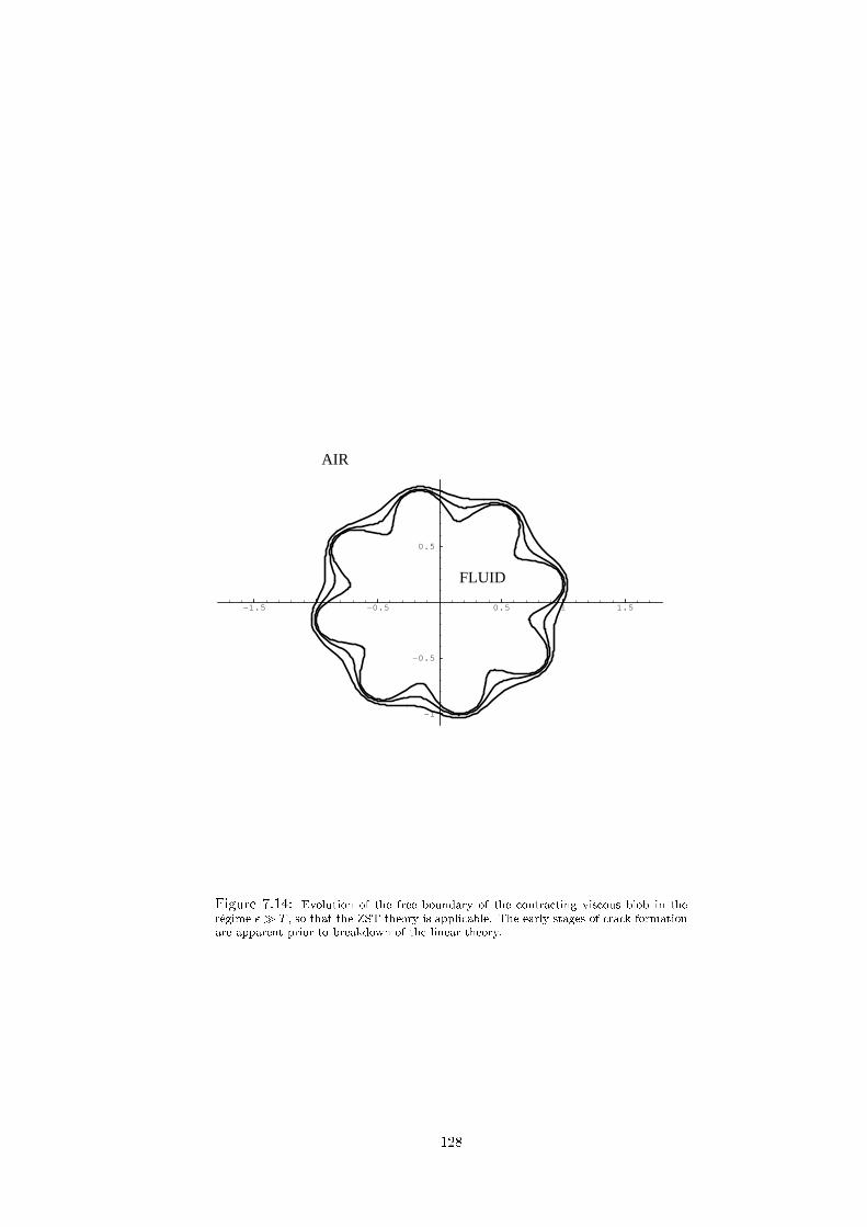
-1.5 -1 -0.5 0.5 1 1.5
-1
-0.5
0.5
1
AIR
FLUID
Figure 7.14: Evolution of the free boundary of the ontra ting vis ous blob in the
r�egime �� T , so that the ZST theory is appli able. The early stages of ra k formation
are apparent prior to breakdown of the linear theory.
128
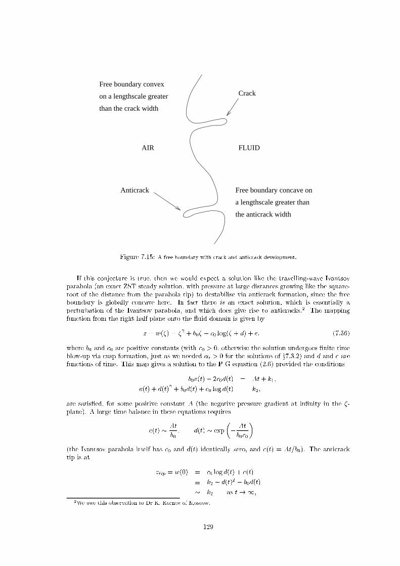
AIR FLUID
Crack
Anticrack
Free boundary convex
on a lengthscale greater
than the crack width
Free boundary concave on
a lengthscale greater than
the anticrack width
Figure 7.15: A free boundary with ra k and anti ra k development.
If this onje ture is true, then we would expe t a solution like the travelling-wave Ivantsov
parabola (an exa t ZST steady solution, with pressure at large distan es growing like the square-
root of the distan e from the parabola tip) to destabilise via anti ra k formation, sin e the free
boundary is globally on ave here. In fa t there is an exa t solution, whi h is essentially a
perturbation of the Ivantsov parabola, and whi h does give rise to anti ra ks.
2
The mapping
fun tion from the right-half plane onto the uid domain is given by
z = w(�) = �
2
+ b
0
� +
0
log(� + d) + e; (7.56)
where b
0
and
0
are positive onstants (with
0
> 0, otherwise the solution undergoes �nite time
blow-up via usp formation, just as we needed �
i
> 0 for the solutions of x7.3.2) and d and e are
fun tions of time. This map gives a solution to the P-G equation (2.6) provided the onditions
b
0
e(t)� 2
0
d(t) = At+ k
1
;
e(t) + d(t)
2
+ b
0
d(t) +
0
log d(t) = k
2
;
are satis�ed, for some positive onstant A (the negative pressure gradient at in�nity in the �-
plane). A large-time balan e in these equations requires
e(t) �
At
b
0
; d(t) � exp
�
�
At
b
0
0
�
(the Ivantsov parabola itself has
0
and d(t) identi ally zero, and e(t) = At=b
0
). The anti ra k
tip is at
z
tip
= w(0) =
0
log d(t) + e(t)
� k
2
� d(t)
2
+ b
0
d(t)
� k
2
as t!1;
2
We owe this observation to Dr K. Kornev of Mos ow.
129

-3 -2 -1 1 2 3
-2
-1.5
-1
-0.5
0.5
1
1.5
2
Anticrack
FLUID
AIR
Figure 7.16: The \Ivantsov" anti ra k solution.
and is thus asymptoti ally stagnant, as we expe t from an anti ra k solution. Thus, if the pa-
rameter
0
is hosen to be small, the free boundary shape (for large times) is approximately a
travelling-wave parabola, with a stagnant, narrow strip of uid left behind along the real axis
(see �gure 7.16). If we had a ZST solution with a onvex paraboli free boundary, our onje ture
suggests that this should lead to usp formation within �nite time, and hen e ra k formation (in
the limit of small positive surfa e tension); however, there is no known exa t solution of the P-G
equation for this geometry.
We should point out that there are de�nite ounter-examples to our onje ture, although it
may be argued that we would not expe t su h solutions to be observed in pra ti e. Firstly, in
[46℄, Howison presents a spe i� ase of the radial �ngering solutions (7.22) of [45℄, whi h is an
expanding bubble solution, yet whi h an lead to �nite-time usp formation (whi h we expe t to
be regularised by ra k formation in the T ! 0 limit). This is a onsequen e of a judi ious hoi e
of mapping parameters and initial onditions, however. In parti ular, the number of �ngers is
hosen as n = 4, whereas in reality the number of �ngers whi h develops is determined by (7.26)
and (7.43). For small values of surfa e tension su h as we have in mind, this will lead to large
values of n, and evolution as in the experiments of [73, 11℄.
There are also exa t ZST \ ontra ting blob" type solutions, driven by a point sink at the
origin, whi h an give rise to anti ra k-type stru tures. These are given by the family of mapping
fun tions from the unit dis ,
w(�) = b� + �
N
X
k=1
$
�k
log(1 + $
k
�); (7.57)
where � is some positive onstant, b(t) and (t) are positive fun tions of time (where 2 (0; 1)),
N is a positive integer, and $ is an N 'th root of unity. This map is a solution of the P-G equation
(2.4) provided the following onditions are satis�ed,
d
dt
(b(b+N� )) = �
Q
�
;
130

-2 -1 1 2
-1.5
-1
-0.5
0.5
1
1.5
Figure 7.17: Anti ra k-type stru ture generated by the map (7.57) with N = 4,
� = 0:2, b(0) = 0:755, (0) = 0:887. We see the onset of uspidal blow-up, after whi h
we expe t ontinuation by ra k or slit evolution towards the point sink.
131

-1 -0.8 -0.6 -0.4 -0.2 0.2
-3
-2
-1
1
2
3
0.2 0.4 0.6 0.8 1
-2
-1
1
2 Crack
FLUID
Anticrack
FLUID
(b)(a)
Figure 7.18: The ra k (a) and anti ra k (b) geometries generated by maps (7.58) and (7.59) with � = 0:1.
b + �
N
X
k=1
$
�k
log(1 +
2
$
k
) = �;
for some onstant �. This an generate evolving free boundaries of the kind in �gure 7.17; however,
these solutions always ultimately blow up via usp formation (at whi h point we expe t the ra k
regularisation to ome into e�e t), and in any ase the T > 0 analysis of x7.8 suggests that ra k
formation is what we expe t to observe in a real \ ontra ting blob" experiment.
7.10 Extremal onformal maps
We now onsider brie y ra k and anti ra k geometries (and their slit and \anti-slit" limits) in
terms of extremal onformal maps, and univalent fun tion theory. Consider mapping the right-half
�-plane onformally onto a uid domain whi h we assume to ontain either a single (stationary,
for simpli ity) ra k, or anti ra k. A ra k an be realised as the image of the right-half �-plane
under the map
z =
p
(� + �)
2
+ 1 (0 < �� 1); (7.58)
(�gure 7.18 (a)) where � is a measure of the ra k thi kness. This map has a uniform limit
� ! 0, whi h gives a so- alled extremal map from the right-half plane onto itself, but with the
slit 0 � x � 1 removed. The term \extremal" indi ates that, although this map is not itself
onformal on the boundary of the domain, <(�) = 0, it is a limit point of some set of maps whi h
are all onformal on <(�) � 0. Hen e in terms of onformal maps, a slit may be viewed as a
straightforward limit of a ra k.
Anti ra ks, on the other hand, do not have a sensible anti-slit limit like this. A typi al anti ra k
geometry is generated by the onformal map
z = � + � log(� + exp(�1=�)) 0 < �� 1; (7.59)
where again, � is a measure of the anti ra k thi kness (�gure 7.18 (b)). This is the kind of free
boundary shape we expe t, from all the exa t ZST anti ra k solutions we found. However, it is
easily seen that this map does not have a uniform limit as �! 0. We an only interpret it when
� > 0, in whi h ase it gives a smooth, narrow anti ra k with tip at x = �1.
Geometri ally, the two ases are fundamentally di�erent. An anti-slit stru ture (of the kind
envisaged in x7.7) annot be realised as a limit point of some set of univalent fun tions in the
132

x
y�
�
U
�
YX
f
�1
(U
�
)
1
1
-1
z
�
(on the upper
side of the slit).
Figure 7.19: The \open sets" interpretation of the slit geometry.
way that a slit map an. To see why this should be so, onsider the topologi al
3
de�nition of
ontinuity, in terms of open sets. A fun tion between topologi al spa es, f : X ! Y , is ontinuous
if and only if the inverse images (under f) of any open sets in Y are also open in X . The topology
of the uid domain (whi h we identify with Y ), and the right-half �-plane (whi h we identify with
X), is just the usual R
2
topology.
Without assuming any parti ular form for a mapping fun tion f between X and Y (but
hypothesising that it be at least ontinuous) we may make the following observations. For the
slit geometry, given a point z
�
on the slit boundary, we an always �nd some semi ir ular open
set U
�
� Y ontaining this point, the inverse image of whi h will also be open in X (�gure 7.19).
Sin e the edges of the slit are the only potential problem points, the fun tion f will be ontinuous
in this ase. For the anti-slit geometry, however, given a point z
�
on the anti-slit itself, the only
kind of open set U
�
� Y whi h also ontains the point is an open interval of points along the slit.
(The anti-slit has the topology of R, rather than of R
2
.) Sin e boundary points map to boundary
points, the inverse image of this interval under the map must also be a line segment along the
imaginary axis in X . Su h a set is not open in the topology of X , sin e we annot �t an `open
ball', around an interior point, within f
�1
(U
�
), and hen e there an exist no ontinuous (and
ertainly no univalent) map between the right-half plane and an anti-slit domain|see �gure 7.20.
We may also interpret this result in terms of the Carath�eodory theorem of kernel onvergen e
(see for instan e [20℄, whose explanation we paraphrase below), a result of major importan e in
geometri fun tion theory. This theorem was also used in relation to the Hele-Shaw problem by
Hohlov & Howison [32℄, to derive estimates for geometri properties of the uid domain in the
inje tion problem. Suppose we have some sequen e of simply- onne ted domains fD
n
g in the
omplex plane, all ontaining some �xed point z
0
(and none of whi h is the entire omplex plane).
Let z = f
n
(�) be the onformal mapping from the right-half �-plane onto D
n
, normalised by the
onditions f
n
(1) = z
0
, f
0
n
(1) > 0. There are two possible ases distinguished by Carath�eodory.
First, suppose that z
0
is an interior point of the interse tion of the D
n
. Then the kernel of the
sequen e fD
n
g is de�ned as the largest domain D whi h ontains z
0
, and whi h has the property
that ea h ompa t subset of D lies in all but a �nite number of the domains D
n
. The other
possibility is that z
0
is not an interior point of the interse tion. In this ase the kernel is de�ned
as D = f0g. In either ase the sequen e fD
n
g is said to onverge to its kernel if every subsequen e
has the same kernel.
3
For more details on pre ise topologi al de�nitions see, for instan e, [92℄.
133

X Y
x
y
�
�
z
�
U
�
f
�1
(U
�
)
(set of boundary points)
Figure 7.20: The \open sets" interpretation of the anti-slit geometry. The `set of boundary points' is not open
in the topology of X.
The basi theorem is as follows [20℄:
Theorem (Carath
�
eodory): Let fD
n
g be a sequen e of simply- onne ted domains,
with z
0
2 D
n
, n = 1; 2; : : :, and suppose f
n
maps the right-half plane X onformally
onto D
n
, and satis�es f
n
(1) = z
0
, f
0
n
(1) > 0. Let D be the kernel of fD
n
g. Then
f
n
! f uniformly on ea h ompa t subset of X if and only if D
n
! D 6= C . In the
ase of onvergen e there are two possibilities.
1. If D = f0g, then f = 0.
2. If D 6= f0g, then D is a simply- onne ted domain, f maps X onformally onto
D, and the inverse fun tions f
�1
n
onverge uniformly to f
�1
on ea h ompa t
subset of D.
With a little modi� ation, the maps (7.58), (7.59) may be made to satisfy the onditions of the
theorem. Taking � to be some fun tion of n whi h tends to zero as n!1 (e.g. � = 1=n will do)
a suitable ra k mapping sequen e is found to be
f
n
(�) =
�
(� + �)
2
+ 1
(1 + �)
2
+ 1
�
1=2
;
whi h has f
n
(1) = 1 for all n, and whi h for small � (large n) des ribes an approximate half-spa e
having a ra k with tip at
f
n
(0) =
1
p
2
�
1�
�
2
+O(�
2
)
�
:
In the notation of the theorem then, z
0
= 1 (the �xed point), whi h lies within the domain D
n
for
all n. The kernel of this sequen e of domains is the right-half plane minus the slit along (0; 1=
p
2),
whi h is exa tly the limit of the image domains D
n
as n!1. The mapping fun tions onverge
uniformly to
f(�) =
p
1 + �
2
p
2
;
134

whi h is the map from X onto the kernel of the domain sequen e, D (de�ned above). Hen e we
have a straightforward example of ase 2 of the theorem.
A suitable anti ra k mapping sequen e is
f
n
(�) =
1
2
�
� � 1 + � log
�
� + exp(�1=�)
1 + exp(�1=�)
��
;
whi h has the �xed (interior) point z
0
= 0 (sin e f
n
(1) = 0 for all n). For small � (large n) these
maps des ribe anti ra k-type stru tures, having anti ra k tips at the points
f
n
(0) = �
1
2
�
�
2
log(1 + exp(1=�)) < �1:
The limiting domain D
1
(whi h is exa tly the interse tion of all the D
n
) is the anti-slit stru ture;
the right-half plane, with an outward-pointing slit along (�1; 0). The �xed point z
0
= 0 is not an
interior point of this interse tion, so the kernel for this sequen e is just D = f0g. Hen e by the
theorem, there is no limiting fun tion f whi h will map X onto the anti-slit stru ture. Re alling
the analysis des ribed in x7.5, this result is not surprising, sin e the results of that se tion strongly
suggest that the orre t \anti-slit" limit will in fa t be an outward-pointing usp, rather than an
outward-pointing slit.
7.11 Summary
Our aim in this hapter has been to present a new theory of anti ra k solutions for the Hele-
Shaw problem, whi h omplements the existing ra k theory of [36, 62, 33℄, reviewed in x7.1.
The omplementary nature of the two is illustrated by pi tures like �gure 7.7. Both ra ks
and anti ra ks may be viewed as regularisations of the ill-posed su tion (or retreating vis ous
boundary) problem, though of very di�erent kinds.
Several exa t ZST anti ra k solutions were given in xx7.3.1, 7.3.2, 7.3.3, but what we termed
the \generi anti ra k" (7.9) aptures all the essentials of the behaviour. Anti ra k tips are
asymptoti ally stagnant (the S hwarz fun tion having a logarithmi singularity within the tip),
while the rest of the anti ra k annot \feel" the tip, and behaves like the travelling-wave solution
(7.14).
The analysis of the expanding bubble problem in x7.6 revealed that sele tion of the anti ra k
width o urs as soon as the instability sets in. On e the anti ra k has formed, it is basi ally
stagnant, and does not in uen e the rest of the free boundary. We summarise this, for a general
situation, by the statement that surfa e tension e�e ts at the anti ra k root govern anti ra k
sele tion. Contrast this with the ra k theory, where it is the surfa e tension e�e ts in the tip
whi h govern the behaviour.
We also saw the ontrast between ra ks and anti ra ks in x7.10. The results there suggest
that, although extremal univalent maps provide a good framework for the ra k/slit theory, they
are not suited to dealing with anti ra k stru tures.
We ited experimental, numeri al, and theoreti al eviden e in support of the ra k and an-
ti ra k theories. In addition, for the anti ra k, there is supporting eviden e from the formal
asymptoti s of [56, 57℄ (x7.5). Based on the analyses of xx7.6 and 7.8, we made a onje ture
to the e�e t that, whether ra k or anti ra k formation o urs may depend on the urvature of
the retreating free boundary. We point out, though, that ra ks must remain as the dominant
stabilising me hanism, in that they are the only omponent of the irregular morphology that an
a�e t the smooth part of the boundary. Anti ra ks do not a�e t it; the free boundary an `sprout'
them, and arry on its way otherwise un hanged.
The overall pi ture we have in mind in this hapter is that the free boundary for a general
su tion problem (with small positive surfa e tension) will be the union of some array of smooth
omponents, ra ks, and anti ra ks (�gure 7.21). Note, however, that for su h a free bound-
ary on�guration to o ur, the anti ra ks must develop �rst, sin e there are three times ales
in operation|anti ra ks are stagnant relative to the motion of the smooth omponents of the
boundary, whi h are themselves stationary relative to the ra k propagation.
135

FLUID
Anticracks
Cracks
AIR
Smoothcomponents
Figure 7.21: The free boundary for a general su tion problem (with small surfa e
tension).
136

Chapter 8
Dis ussion and further work
8.1 Comparison of Hele-Shaw and Stokes ow
One of our aims in this thesis has been to highlight the similarities and di�eren es between Hele-
Shaw ow and Stokes ow. Although we have mentioned su h points of omparison as they
o urred, it is helpful to summarise and dis uss them here.
� Both Hele-Shaw and Stokes ow are quasistati free boundary problems, by whi h we mean
that the time dependen e enters the problem only through the kinemati boundary ondi-
tion.
� Both are governed by ellipti p.d.e.'s; the pressure �eld for Hele-Shaw is harmoni , and the
streamfun tion for Stokes ow is biharmoni . (Note that in Hele-Shaw, sin e the pressure
is a velo ity potential for the ow, its harmoni onjugate is a streamfun tion, whi h is also
harmoni .) Both problems are thus amenable to atta k by similar omplex variable methods.
In general, one might expe t a se ond-order p.d.e. to be simpler than a fourth-order one,
but as we have seen in hapters 2 and 3, the NZST Stokes ow problem is very mu h
more tra table analyti ally than the NZST Hele-Shaw problem. Re all, in this ontext, the
omments of x3.6.2, where we stated that the mapping fun tion whi h gives a solution to
the ZST Stokes ow problem will also give a solution to the NZST problem, but the same
is not true for the Hele-Shaw problem.
Although it is more usual to onsider the surfa e tension driven Stokes ow problem, with a velo -
ity �eld whi h is everywhere analyti (sin e this arises in real-world situations su h as sintering),
mu h of the work in this thesis has been for the singularity driven ZST problem, whi h is the
usual Hele-Shaw s enario. We have thus been able to make dire t omparison between the two.
� In x5.4.2 we have stated that with one te hni al assumption �(0) = 0 (for Stokes ow), the
same onformal map will yield solutions for both the Hele-Shaw and Stokes ow problems
(ZST, and singularity-driven) in the same geometry. However, we also saw that if we have
more than one singularity in the ow (in luding singularities at in�nity), the Stokes ow
solution will, in general, be diÆ ult to realise in pra ti e, having moving singularities. This
is not the ase for Hele-Shaw ow; the basi reason (as dis ussed in x5.1) is that the S hwarz
fun tion evolution for Stokes ow is determined in the �-plane, while for Hele-Shaw it is
determined in the physi al plane. Hen e only for Hele-Shaw ow an we expe t to be able
to mat h the singularities of the S hwarz fun tion with those of the ow.
� Both ZST problems are time-reversible. From this one may dedu e that for both problems
a ontra ting vis ous blob, unless it is a ir le with su tion from the origin, must undergo
�nite time blow-up before all uid has been extra ted.
137

� It is a simple matter to demonstrate that a ZST Hele-Shaw ow with an advan ing/retreating
vis ous boundary, is stable/unstable, respe tively (the latter, whi h we loosely refer to as
the Hele-Shaw su tion problem, is well known to be ill-posed). By ontrast, Stokes ow is
neutrally stable to rigid-body motions, and the question of stability of advan ing/retreating
vis ous boundaries does not arise. However, we are able to analyse nearly- ir ular \bubbles"
and \blobs" in ZST Stokes ow, and we �nd that an expanding/ ontra ting bubble or blob
is stable/unstable respe tively (see appendix A). For Hele-Shaw ow, the above stability
result means that a ontra ting/expanding bubble is stable/unstable respe tively, while an
expanding/ ontra ting blob is stable/unstable respe tively (see xx7.6, 7.8). The Hele-Shaw
instability is mu h more dramati than the Stokes ow, as omparison of (7.38) and (7.52)
(with � = 0, and for large n) with (A.6) and (A.3) shows.
Our belief is that the ZST Hele-Shaw instability leads to either anti ra k formation, or �nite-
time blow-up via usp formation or self-overlapping of the free boundary. It is thought that
the only possibilities for Stokes ow are the latter two; no examples of Stokes anti ra ks are
known.
� In the ase of 3/2-power uspidal blow up (whi h is always terminal for the ZST problems),
the behaviour of the velo ity �elds at the usp as the blow up time t
�
is approa hed is very
di�erent in the two ases. In Hele-Shaw, the velo ity be omes unbounded; for a ontra ting
vis ous blob of the kind onsidered in [49℄, the speed at the usp behaves like
speed �
1
p
t
�
� t
as t! t
�
;
while for Stokes ow,
speed � O(1) as t! t
�
:
� For 5/2-power uspidal blow-up it is possible for the solution to evolve through the usped
on�guration. An example of this behaviour for ZST Hele-Shaw ow arose in x5.3 (and many
others exist in the literature); for NZST Stokes ow see [85℄|we do not give an example
in this thesis. Note though, that in the ubi polynomial example of x6.2, 5/2-power usp
formation is terminal for the ZST Stokes ow problem, whereas for the analogous Hele-Shaw
problem, it is not [50℄. Our results there show that in the T ! 0 limit, the 5/2-power usp
be omes a 3/2-power usp, although it is a borderline ase. It is possible that nonzero
surfa e tension is ne essary to have ontinuable uspidal solutions (meaning that the free
boundary be nonanalyti only for an instant, before smoothing again) for the Stokes ow
problem.
� For both problems, a T ! 0 regularisation may be onsidered. For Stokes ow we saw
that this leads to solutions whi h have persistent usps in the free boundary ( hapter 6, the
\weak solution" on ept). For Hele-Shaw, the onje tured s enario is the slit model ( hapter
7), with an air slit propagating into the uid domain from the usp, moving in�nitely fast
relative to the rest of the free boundary. Note that \weak" Stokes ow solutions are not
time reversible, as the usped \similarity" solutions of [49℄ demonstrate. A time-reversal
for slit solutions an be proposed, however, sin e we would expe t the slit to ontra t ba k
along its length to the usp, after whi h the free boundary would instantly smooth, and
lassi al theory take over.
One of the most striking similarities between the two problems is the existen e of the \moments",
whi h obey the same evolution equations for the point sink (or sour e) problem, although they
are di�erently de�ned (xx2.5, 3.6, 3.6.2).
Underlying this di�eren e in de�nition is the fa t that the singularities of the S hwarz fun tion
for Hele-Shaw are determined in the physi al domain, whereas for Stokes ow (in the ase �(0) = 0)
they are determined within the unit dis in �-spa e. Re all the reper ussions that this had for
138

many-singularity problems: the ZST Hele-Shaw results are readily extended to ope with su h
problems, but the Stokes ow results are not.
Another analogy between the two problems is the existen e of a Baio hi transform for ea h
(xx2.6, 3.9.1). Again these are di�erently de�ned; like the \moments", the integrals in the de�ni-
tions are arried out in physi al spa e for Hele-Shaw, and in �-spa e for Stokes ow.
8.2 Further work
At some points in this thesis we have been unable to omplete the solution to parti ular problems.
In other pla es we hose to leave a problem at a ertain stage, when the work ould have been
extended in various dire tions. We list below some of the more interesting and important areas
for future study related to the work of the thesis.
1. We have seen that, unlike the ZST Hele-Shaw theory, the ZST Stokes ow theory of hapter 3
an only deal with many driving singularities (or singularity-driven problems on unbounded
domains) if we allow them to move, leading to solutions whi h are somewhat ontrived.
Essentially the same diÆ ulty arose in x5.4.2 where, to avoid a moving singularity, we
required the solution to have �(0) 6= 0. This led to a very ompli ated formula for the
onformal map, and we were unable to solve the problem fully. It is possible that there is a
better way of atta king su h problems (perhaps not involving omplex variable methods?).
Further investigation is needed if we are to develop a omprehensive theory to deal with
time-dependent problems of this kind (note that the existing methods are perfe tly adequate
for steady problems).
2. It was mentioned in x8.1 above that although Hele-Shaw slit solutions are reversible in time,
the \weak" similarity solutions of [49℄, with persistent usps, are not|would inje tion into
a usped on�guration give an expanding usped shape of similarity type, or would the free
boundary smooth instantly? This is an interesting open question, and may be ompared
with the Hele-Shaw results of [56℄, where weak solutions to the inje tion problem (with
an a ute-angled orner in the initial free boundary) are found to exhibit \waiting time"
behaviour. In su h solutions, the orner persists for the waiting time, at whi h the orner
angle jumps to its supplement, then instantaneously smooths.
3. Re all the omment in footnote (3) of hapter 3, that the governing equations (3.18) have
the form of a general onservation law. This enables a possible weak formulation to be
written down, whi h we did not pursue. It would be interesting to investigate this point
further, in parti ular, to see if it an be linked to the \weak solution" theory of hapter 6.
It is possible that the ZST breakdown time t = t
�
may be asso iated with a sho k surfa e,
a ross whi h the form of the solution hanges, and that Rankine-Hugoniot onditions may
be asso iated with persistent usps. This suggestion is highly spe ulative as yet.
4. The ra k/anti ra k theory of hapter 7 is in omplete. More work needs to be done on the
ra k and slit theories, whi h were already known to be ill-posed and under-determined,
respe tively (and whi h we did not attempt to extend). Although we saw how the anti ra k
\sele tion at the root" worked for the expanding bubbles and ontra ting blobs of Paterson's
experiments [73℄, we do not yet have a full understanding of the role played by surfa e tension
in general anti ra k solutions, and in parti ular, we do not have a lear idea of what we
expe t in the T ! 0 limit (if ra ks be ome slits, what do anti ra ks be ome? Se tion 7.10
implies that the theory of extremal univalent maps annot help us in this ase). Finally,
although in x7.9 we onje ture that the urvature of the free boundary may determine whi h
parti ular instability is observed in a given situation, this is still a very tentative suggestion,
whi h needs ba king up with some hard eviden e.
139

Appendix A
Stability of blobs and bubbles in
Stokes ow
In this appendix we show how omplex variable methods may be used to perform a simple linear
stability analysis of expanding and ontra ting ir ular blobs and bubbles in ZST Stokes ow. We
use known, exa t solutions, in a suitable small parameter limit, to dedu e our stability results.
A.1 The perturbed ir ular blob
Howison & Ri hardson [49℄ presented exa t solutions for the sour e or sink driven evolution of a
vis ous blob, des ribed by the onformal map
z = w(�) = a(� �
b
n
�
n
);
for positive integer n, and time-dependent parameters a and b whi h may both be assumed real
and positive by a suitable hoi e of axes. The equations governing the ZST evolution of a and b
are given as
a
2
b = k; (A.1)
dS
dt
=
d
dt
�
�a
2
�
1 +
b
2
n
��
= �Q; (A.2)
for some positive onstant k. Here, S(t) denotes the area of the uid domain, so Q > 0 for a
point sink at the origin, and Q < 0 for a sour e. If we onsider the ase b = � � 1, then on the
free boundary,
jzj = a(1�
�
n
os(n� 1)� +O(�
2
));
whi h is just a sinusoidal perturbation to an expanding or ontra ting ir ular blob (i.e. linear
stability theory).
To lowest order, (A.1) and (A.2) give the solution for �(t) as
�(t) =
�k
S(t)
: (A.3)
Hen e we see that � is growing in time for a point sink (S(t) de reasing), whi h means an unstable
situation, and de reasing in time for a point sour e, i.e. a stable situation, the growth or de ay
being algebrai in t. Thus for vis ous blobs, we have the same situation as for Hele-Shaw ow
(see x7.8).
140

A.2 The perturbed ir ular bubble
The analogous bubble problem was solved by Tanveer & Vas on elos [96℄. The onformal map
for this ase is
z = w(�) = a
�
1
�
�
�
n
�
n
�
;
for positive integer n, where again a > 0 and 0 < �� 1. The free boundary here is su h that
jzj = a(1�
�
n
os(n+ 1)� +O(�
2
));
and the ZST equations governing the parameters are
a
2
� = k; (A.4)
dB
dt
=
d
dt
�
�a
2
�
1�
�
2
n
��
= Q; (A.5)
for some positive onstant k, where now B(t) denotes the bubble area, so Q > 0 for a sink at
in�nity, i.e. a growing bubble, and Q < 0 for a shrinking bubble. Combining (A.4) and (A.5)
gives the evolution of �(t) (to lowest order) as
�(t) =
�k
B(t)
; (A.6)
so a growing bubble is stable (� de reasing), while a shrinking bubble is unstable. This result is
in dire t ontrast to the orresponding Hele-Shaw result of x7.6, where we saw that expanding
bubbles are unstable (giving rise to anti ra ks), while ontra ting bubbles are stable.
141

Appendix B
Results used for the ubi
polynomial map
In this Appendix we give the exa t and asymptoti expressions for the fun tions f
+
(0; t) and
f
0
+
(0; t) whi h we omitted from the text in hapter 6.
Using the de�nition (3.8) we �nd
f
+
(0) �
1
�a
Z
�
0
d�
[b
2
+ ( � 1)
2
+ 2b(1 + ) os � + 4 os
2
�℄
1=2
;
and f
0
+
(0) �
1
�a
Z
�
0
os � d�
[b
2
+ ( � 1)
2
+ 2b(1 + ) os � + 4 os
2
�℄
1=2
;
the forms of whi h fun tions hange as we ross the urve b
2
= 4 in V (a ording to whether the
denominator has real or omplex roots as a fun tion of os �); f
+
(0) itself is ontinuous a ross
this urve, however. In b
2
< 4 we use formula 3.145.2 in Gradshteyn & Ryzhik [30℄ (hen eforth
G & R), and also the asymptoti result
K(1� �) � �
1
2
log(�=8) � �
1
2
log � as �! 0; (B.1)
where K( � ) is the omplete ellipti integral of the �rst kind. We �nd that
f
+
(0) =
2K(k
1
)
�a
p
( + 1)
2
� b
2
; where k
2
1
:=
4 � b
2
( + 1)
2
� b
2
;
�
�2
�a
p
4� b
2
log(1� ) as " 1;
= 1 being the only singularity within this part of V . In b
2
> 4 we need formulae 3.147.6 and
3.147.4 of G & R (in regions > 0, < 0 respe tively) together with (B.1) to dedu e that
f
+
(0) =
2K(k
2
)
�a
�
p
b
2
� 4 + (1� )
�where k
2
2
:=
4(1� )
p
b
2
� 4
[
p
b
2
� 4 + (1� )℄
2
�
�1
�a(1� )
log(1 + � b) as (1 + � b) # 0;
b = 1 + now being the only line of singularities within V . Expli it formulae for f
0
+
(0) are mu h
more ompli ated; in b
2
< 4 we �nd
f
0
+
(0) =
�b(1 + )K(k
1
)
2�a
p
(1 + )
2
� b
2
+
1
p
fE(k
1
)F ( ; k
0
1
) +K(k
1
)(E( ; k
0
1
)� F ( ; k
0
1
))g ;
where (k
0
1
)
2
= 1� k
2
1
; = sin
�1
(
b
2
p
); (B.2)
142

here k
1
is as previously de�ned, E( � ); E( � ; � ) denote the omplete and in omplete (respe tively)
ellipti integrals of the se ond kind, and F ( � ; � ) denotes the in omplete ellipti integral of the
�rst kind (so K( � ) � F (�=2; � )). The key formulae used in �nding this expression were 259.07
and 410.02 in Byrd & Friedman [8℄ (hen eforth B & F), along with various properties of ellipti
integrals and Ja obian ellipti fun tions, all of whi h may be found in B & F.
In b
2
> 4 we �nd
f
0
+
(0) =
2
�a(
p
b
2
� 4 + (1� ))
�
AK(k
2
)� (1 +A)�
�
2
1�A
; k
2
��
;
where A =
1
4
�
�b(1 + ) + (1� )
p
b
2
� 4
�
; (B.3)
again, k
2
is as previously de�ned, and �( � ; � ) denotes the omplete ellipti integral of the third
kind. In �nding this expression the formulae used were G & R 3.148.6 and 3.148.4 (in regions
> 0 and < 0 respe tively).
In using these two books, are was ne essary to a ount for slight di�eren es in de�nitions.
Likewise, when arrying out numeri al he ks on the analysis, are was needed due to di�erent
inbuilt de�nitions in the software pa kage Mathemati a. The above assumes the de�nitions:
F (�; k) =
Z
�
0
d�
p
1� k
2
sin
2
�
=
Z
sin�
0
dx
p
(1� x
2
)(1� k
2
x
2
)
; (B.4)
E(�; k) =
Z
�
0
p
1� k
2
sin
2
� d� =
Z
sin�
0
p
1� k
2
x
2
p
1� x
2
dx ;
�(�
2
; k) =
Z
�=2
0
d�
(1� �
2
sin
2
�)
p
1� k
2
sin
2
�
=
Z
1
0
dx
(1� �
2
x
2
)
p
(1� x
2
)(1� k
2
x
2
)
:
The results of x6.2 require the asymptoti evaluation of the ratio f
0
+
(0)=f
+
(0) near ea h of the
lines = 1 and b = 1 + . This is not too bad for the ase " 1, and fairly nasty for the ase
b # (1 + ); we give only brief details.
In b
2
< 4 results of B & F xx111{112 are used, together with (B.1) above, to dedu e that as
" 1, the term in urly bra kets in G
0
+
(0) (B.2) is everywhere negligible ompared to the �rst
term. Hen e we see that the asymptoti behaviour here is
f
0
+
(0)
f
+
(0)
� �
b
2
: (B.5)
To study the behaviour of f
0
+
(0) as b " (1 + ) in the region b
2
> 4 we must onsider the
ases > 0 and < 0 separately, sin e these give di�erent types of behaviour in (B.3). We write
� = 1+ �b and eliminate b to work with and �, so that letting �! 0 orresponds to approa hing
the univalen y boundary �V . We also de�ne the auxiliary parameter Æ := �
2
=(4(1� )
2
); this will
always be small sin e we do not onsider the ellipti al part of �V orresponding to blow-up via
overlapping of the free boundary, so lies in the range �1 < < 3=5. We �nd:
A = �1� 2Æ + � � � ; �(1 +A) = 2Æ + � � � ;
k
2
2
= 1� Æ
�
1 +
1�
�
2
+ � � � ; �
2
�
2
1�A
= 1� Æ + � � � :
We know the asymptoti behaviour of the �rst term in urly bra kets in f
0
+
(0) (B.3), from (B.1).
The term outside, multiplying the urly bra ket, is also straightforward. Hen e we only need to
�nd the behaviour of the se ond term within urly bra kets, whi h to lowest order is
�(1 +A)�
�
2
1�A
; k
2
�
� 2�(�
2
; k
2
):
143

Suppose �rst that 2 (0; 3=5). Then by the above expressions, 0 < �
2
< k
2
2
< 1, and so a ording
to the lassi� ations of B & F (p. 223) we have a ase II ellipti integral of the third kind (a
ir ular ase).
1
Formula 412.01 in B & F thus applies, giving the result in terms of the Heuman
Lambda fun tion. Results from x150 of the book may then be used to arrive at the approximation
2�(�
2
; k
2
) =
1�
p
�
�
2
� sin
�1
�
1�
1 +
��
+O(Æ log Æ);
whi h gives ex ellent agreement when he ked numeri ally. This term will thus be everywhere
negligible ompared to the �rst term in the urly bra kets (K(k
2
) being singular as k
2
! 1),
hen e we get the approximation
f
0
+
(0) �
1
�a(1� )
log(1 + � b):
It follows that for in this parameter range we will have
f
0
+
(0)
f
+
(0)
� �1;
as we approa h the boundary.
For 2 (�1; 0) (still using (B.3)) we have 0 < k
2
2
< �
2
< 1, whi h is a ase III ellipti integral
of the third kind (a hyperboli ase). Thus formula 414.01 of B & F applies, and it is relatively
easy to see that
2�(�
2
; k
2
) '
1�
p
�
K(k
2
)Z(�; k
2
) for � = sin
�1
�
�
k
2
�
=
�
2
�
2
p
� Æ
1�
+ � � � ;
where Z( � ; � ) denotes the Ja obi Zeta fun tion (dis ussed in x140 of B & F). Then
f
0
+
(0) �
�K(k
2
)
�a(1� )
�
1�
1�
p
�
Z(�; k
2
)
�
;
so that
f
0
+
(0)
f
+
(0)
� �1 +
1�
p
�
Z(�; k
2
):
Results of x140 and x100 in B & F show that for small Æ,
Z(�; k
2
) �
1
K(k
2
)
log
2
p
�
1 +
+
�
1�
4
(1 + )
2
�
1=2
!
:
Note that = 0 is not a problem point, despite the fa tor 1=
p
� in the above, be ause for small
we may expand the logarithmi term appearing in the expression for Z(�; k
2
). The only problem
is at = �1; away from this point we an see that
f
0
+
(0)
f
+
(0)
� �1:
Near = �1, the fun tion Z(�; k
2
) will no longer be negligible a ording to the above. Here we
have
f
0
+
(0)
f
+
(0)
� �1 + 2
�
1 +
log �
log(1 + )
�
�1
= �1 + 2
�
1 +
log �
log(�+ b)
�
�1
;
1
The ase = 0 is the spe ial ase �
2
= k
2
, and provides a he k on the analysis in both regions > 0, < 0.
144

for lose to �1 (or, b small and positive). So, for instan e, if we take b = �� for some order one
quantity � we will have
f
0
+
(0)
f
+
(0)
! 0 as �! 0:
In parti ular, this will be the ase as we approa h the univalen y boundary along the phase path
b � 0. We thus have a nonuniform limit, with
f
0
+
(0)
f
+
(0)
! �1 as �! 0 (B.6)
everywhere ex ept = �1 (or b = 0); at this point the limit is zero.
145
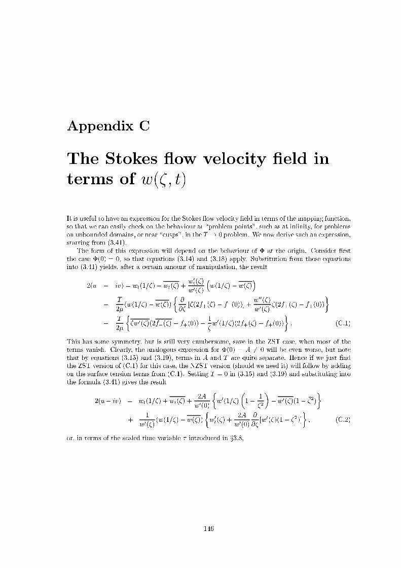
Appendix C
The Stokes ow velo ity �eld in
terms of w(�; t)
It is useful to have an expression for the Stokes ow velo ity �eld in terms of the mapping fun tion,
so that we an easily he k on the behaviour at \problem points", su h as at in�nity, for problems
on unbounded domains, or near \ usps", in the T ! 0 problem. We now derive su h an expression,
starting from (3.41).
The form of this expression will depend on the behaviour of � at the origin. Consider �rst
the ase �(0) = 0, so that equations (3.14) and (3.18) apply. Substitution from these equations
into (3.41) yields, after a ertain amount of manipulation, the result
2(u � iv) = �w
t
(1=�) + w
t
(�) +
w
0
t
(�)
w
0
(�)
�
�w(1=�)� w(�)
�
�
T
2�
( �w(1=�)� w(�))
�
�
��
[�(2f
+
(�) � f
+
(0))℄ +
w
00
(�)
w
0
(�)
�(2f
+
(�)� f
+
(0))
�
+
T
2�
�
�w
0
(�)(2f
+
(�) � f
+
(0))�
1
�
�w
0
(1=�)(2f
+
(�) � f
+
(0))
�
: (C.1)
This has some symmetry, but is still very umbersome, save in the ZST ase, when most of the
terms vanish. Clearly, the analogous expression for �(0) = A 6= 0 will be even worse, but note
that by equations (3.15) and (3.19), terms in A and T are quite separate. Hen e if we just �nd
the ZST version of (C.1) for this ase, the NZST version (should we need it) will follow by adding
on the surfa e tension terms from (C.1). Setting T = 0 in (3.15) and (3.19) and substituting into
the formula (3.41) gives the result
2(u� iv) = �w
t
(1=�) + w
t
(�) +
2A
w
0
(0)
�
�w
0
(1=�)
�
1�
1
�
2
�
+ w
0
(�)(1�
�
�
2
)
�
+
1
w
0
(�)
( �w(1=�)� w(�))
�
w
0
t
(�) +
2A
w
0
(0)
�
��
[w
0
(�)(1� �
2
)℄
�
; (C.2)
or, in terms of the s aled time variable � introdu ed in x3.8,
146

w
0
(0)
A
(u� iv) = �w
�
(1=�) + w
�
(�) +
�
�w
0
(1=�)
�
1�
1
�
2
�
+ w
0
(�)(1�
�
�
2
)
�
+
1
w
0
(�)
( �w(1=�)� w(�))
�
w
0
�
(�) +
�
��
[w
0
(�)(1 � �
2
)℄
�
: (C.3)
147

Referen es
[1℄ A rivos, A. The breakup of small drops and bubbles in shear ows. Ann. N.Y. A ad. S i.
404, 1-11 (1983).
[2℄ Antanovskii, L.K. In uen e of surfa tants on a reeping free boundary ow indu ed by
two ounter-rotating horizontal thin ylinders. Eur. J. Me h. B/Fluids 13 (1), 73-92 (1994).
[3℄ Antanovskii, L.K. A plane invis id in ompressible bubble pla ed within a reeping vis ous
ow: formation of a usped bubble. Eur. J. Me h. B/Fluids 13 (4), 491-509 (1994).
[4℄ Antanovskii, L.K. Mathemati al modelling of formation of a pointed drop in a four-roll
mill. Preprint (1995).
[5℄ Baio hi, C. Ann. Mat. Pura. Appl. 92, 107-127 (1972).
[6℄ Bat helor, G.K. An introdu tion to Fluid Dynami s. C.U.P. (1967).
[7℄ Bu kmaster, J.D. Pointed bubbles in slow vis ous ow. J. Fl. Me h. 55, 385-400 (1972).
[8℄ Byrd, P.F., Friedman, M.D. Handbook of Ellipti Integrals for Engineers and S ientists.
Springer-Verlag (1971).
[9℄ Caginalp, G. Stefan and Hele-Shaw type models as asymptoti limits of the phase �eld
equations. Phys. Rev. A 39, 5887 (1989).
[10℄ Carrier, G.F., Krook, M., Pearson, C.E. Fun tions of a Complex Variable. Hod Press:
Itha a, New York (1983).
[11℄ Chen, J.-D. Growth of radial vis ous �ngers in a Hele-Shaw ell. J. Fl. Me h. 201, 223-242
(1989).
[12℄ Chen, X., Hong, J., Yi, F. Existen e, uniqueness and regularity of lassi al solutions of
the Mullins-Sekerka problem. Preprint (1996).
[13℄ Combes ot, R., Hakim, V., Dombre, T., Pomeau, Y., Pumir, A. Shape sele tion for
Sa�man-Taylor �ngers. Phys. Rev. Lett. 56, 2036-2039 (1986).
[14℄ Couder, Y., G
�
erard, N., Rabaud, M. Narrow �ngers in the Sa�man-Taylor instability.
Phys. Rev. A { General Physi s 34 (6), 5175-5178 (1986).
[15℄ Cowling, V.F., Royster, W.C. Domains of variability for univalent polynomials. Pro .
Amer. Math. So . 19, 767-772 (1968).
[16℄ Crowdy, D.G., Tanveer, S. A theory of exa t solutions for plane vis ous blobs. Preprint
(1996).
[17℄ Davis, P.J. The S hwarz fun tion and its appli ations. Carus Math. Monographs 17, Math.
Asso . of Ameri a (1974).
148

[18℄ DiBenedetto, E., Friedman, A. The ill-posed Hele-Shaw model and the Stefan problem
for super ooled water. Trans. Am. Math. So . 282, 183-204 (1984).
[19℄ Du hon, J., Robert, R. Interfa e evolution by apillarity and volume di�usion (1). Ex-
isten e lo ally in time. Annales de l'Institute Henri Poin ar�e|Analyse non-lineaire 1 (5),
361-378 (1984).
[20℄ Duren, P.L. Univalent fun tions. Springer-Verlag (1983).
[21℄ Elliott, C.M., Janovsky, V. A variational inequality approa h to Hele-Shaw ow with
a moving boundary. Pro . Roy. So . Edin. A88, 93-107 (1981).
[22℄ Elliott, C.M., O kendon, J.R. Weak and variational methods for moving boundary
problems. Pitman, London (1982).
[23℄ Elliott, C.M., Gardiner, A.R. Double obsta le phase �eld omputations of dendriti
growth. Preprint (1996).
[24℄ Entov, V.M., Etingof, P.I., Kleinbo k, D.Ya. Hele-Shaw ows with a free boundary
produ ed by multipoles. Euro. J. Appl. Math. 4, 97-120 (1993).
[25℄ Entov, V.M., Etingof, P.I., Kleinbo k, D.Ya. On nonlinear interfa e dynami s in
Hele-Shaw ows. Euro. J. Appl. Math. 6 (5), 399-420 (1996).
[26℄ Es her, J., Simonett, G. On Hele-Shaw models with surfa e tension. Math. Resear h
Letters (to appear).
[27℄ Es her, J., Simonett, G. Classi al solutions of multi-dimensional Hele-Shaw models.
S.I.A.M. Jl. Math. Anal. (to appear).
[28℄ Galin, L.A. Unsteady �ltration with a free surfa e. Dokl. Akad. Nauk. S.S.S.R. 47, 246-249
(1945).
[29℄ Garabedian, P.R. Free boundary ows of a vis ous liquid. Comm. Pure & Appl. Math.
XIX (4), 421-434 (1966).
[30℄ Gradshteyn, I.S., Ryzhik, I.M. Table of Integrals, Series and Produ ts ( orre ted and
enlarged edition). A ademi Press, in . (1980).
[31℄ Hele-Shaw, H.S. The ow of water. Nature, 58 (1489), 34-36 (1898).
[32℄ Hohlov, Yu.E., Howison, S.D.On the lassi� ation of solutions to the zero surfa e tension
model for Hele-Shaw free boundary ows. Quart. Appl. Math. 51 (4), 777-789 (1993).
[33℄ Hohlov, Yu.E., Howison, S.D., Huntingford, C., O kendon, J.R., La ey, A.A. A
model for non-smooth free boundaries in Hele-Shaw ow. Q. Jl. Me h. Appl. Math. 47 (1),
107-128 (1994).
[34℄ Hong, D.C., Langer, J.S. Analyti theory for the sele tion of Sa�man-Taylor �ngers.
Phys. Rev. Lett. 56, 2032-2035 (1986).
[35℄ Howison, S.D., O kendon, J.R., La ey, A.A. Singularity development in moving
boundary problems. Q. Jl. Me h. Appl. Math. 38 (3), 343-360 (1985).
[36℄ Howison, S.D., La ey, A.A. O kendon, J.R. Hele-Shaw free boundary problems with
su tion. Q. Jl. Me h. Appl. Math. 41, 183-193 (1988).
[37℄ Hopper, R.W. Coales en e of two equal ylinders: Exa t results for reeping vis ous plane
ow driven by apillarity. J. Am. Ceram. So . (Comm.) 67, C262-264. Errata, ibid. 68, C138
(1985).
149

[38℄ Hopper, R.W. Plane Stokes ow driven by apillarity on a free surfa e. J. Fl. Me h. 213,
349-375 (1990).
[39℄ Hopper, R.W. Stokes ow of a ylinder and half-spa e driven by apillarity. J. Fl. Me h.
243, 171-181 (1992).
[40℄ Hopper, R.W. Capillarity-driven plane Stokes ow exterior to a parabola. Q. Jl. Me h.
Appl. Math. 46, 193-210 (1993).
[41℄ Howard, G.C., Fast, C.R. Hydrauli Fra turing. So . Petrol. Eng., AIME, Dallas, TX.
(1970).
[42℄ Howell, P.D. Extensional thin layer ows. D. Phil. Thesis, University of Oxford (1994).
[43℄ Howell, P.D. The evolution of a slender bubble with ellipti al ross-se tion in an exten-
sional ow. (In preparation) (1996).
[44℄ Howison, S.D. Private ommuni ation (1995).
[45℄ Howison, S.D. Fingering in Hele-Shaw ells. J. Fl. Me h. 167, 439-453 (1985).
[46℄ Howison, S.D. Cusp development in Hele-Shaw ow with a free surfa e. S.I.A.M. Jl. Appl.
Math. 46 (1), 20-26 (1986).
[47℄ Howison, S.D. Bubble growth in porous media and Hele-Shaw ells. Pro . Roy. So . Edin.
A. 102, 141-148 (1986).
[48℄ Howison, S.D. Complex variable methods in Hele-Shaw moving boundary problems. Europ.
J. Appl. Math. 3, 209-224 (1992).
[49℄ Howison, S.D., Ri hardson, S. Cusp development in free boundaries, and two-
dimensional slow vis ous ows. Europ. J. Appl. Math. (1995).
[50℄ Huntingford, C. An exa t solution to the one-phase zero surfa e-tension Hele-Shaw free-
boundary problem. Computers Math. Appli . 29 (10), 45-50 (1995).
[51℄ Ivantsov, G.P. Dokl. Akad. Nauk. S.S.S.R. 58, 567 (in Russian) (1947).
[52℄ Jeong, J., Moffatt, H.K. Free-surfa e usps asso iated with ow at low Reynolds number.
J. Fl. Me h. 241, 1-22 (1992).
[53℄ Joseph, D.D., Nelson, J., Renardy, M., Renardy, Y. Two-dimensional usped inter-
fa es. J. Fl. Me h. 223, 383-409 (1991).
[54℄ Kelly, E.D., Hin h, E.J. Numeri al solutions of Entov's multipole problem in the Hele-
Shaw ell. Submitted to Europ. J. Appl. Math. (1995).
[55℄ Kelly, E.D., Hin h, E.J. Numeri al simulations of sink ow in the Hele-Shaw ell with
small surfa e tension. Submitted to Europ. J. Appl. Math. (1996).
[56℄ King, J.R., La ey, A.A., Vazquez, J.L. Persisten e of orners in free boundaries in
Hele-Shaw ow. Europ. J. Appl. Math. 6 (5), 455-490 (1995).
[57℄ King, J.R. Development of singularities in some moving boundary problems Europ. J. Appl.
Math. 6 (5), 491-507 (1995).
[58℄ King, J.R. Private ommuni ation (1995).
[59℄ Kopf-Sill, A.R., Homsy, G.M. Narrow �ngers in a Hele-Shaw ell. Phys. Fluids 30 (9),
2607-2609 (1987).
150
[60℄ La ey, A.A. Moving boundary problems in the ow of liquid through porous media. Jl.
Austral. Math. So . B24, 171-193, (1982).
[61℄ La ey, A.A. I.M.A.J. Appl. Math. 35, 357-364 (1985).
[62℄ La ey, A.A., Howison, S.D., O kendon, J.R., Wilmott, P. Irregular morphologies in
unstable Hele-Shaw free boundary problems. Q. Jl. Me h. Appl. Math. 43, 387-405 (1990).
[63℄ Langlois, W.E. Slow Vis ous Flow. Ma millan (1964).
[64℄ Mallet-Paret, J. Generi unfoldings and normal forms of some singularities arising in the
obsta le problem. Duke Math. J. 46, 645-683 (1979).
[65℄ M Lean, J.W., Saffman, P.G. The e�e t of surfa e tension on the shape of �ngers in a
Hele-Shaw ell. J. Fl. Me h. 102, 455-469 (1981).
[66℄ Mineev-Weinstein, M.B., Pon e-Dawson, S. Class of nonsingular exa t solutions for
Lapla ian pattern formation. Phys. Review E 50 (1), 24-27 (1994).
[67℄ Morgan, J.D. Codimension-Two free boundary problems. D. Phil. Thesis, University of
Oxford (1994).
[68℄ Nehari, Z. Conformal Mapping. Dover (1975).
[69℄ Nie, Q., Tian, F.R. Singularities in Hele-Shaw ows. Submitted to SIAM J. Appl. Math.
(1996).
[70℄ Nie, Q., Tanveer, S. The evolution of an axisymmetri Stokes bubble with volumetri
hange. Submitted to Phys. Fluids (1996).
[71℄ O kendon, H., O kendon, J.R. Vis ous Flow. C.U.P. (1995).
[72℄ Pamplin, B.R. Crystal Growth. Pergamon, Oxford (1975).
[73℄ Paterson, L. Radial �ngering in a Hele-Shaw ell. J. Fl. Me h. 113, 513-529 (1981).
[74℄ Pitts, E. Penetration of uid into a Hele-Shaw ell: the Sa�man-Taylor experiment. J. Fl.
Me h. 97, 53-64 (1980).
[75℄ Polubarinova-Ko hina, P.Ya. On the motion of the oil ontour. Dokl. Akad. Nauk.
S.S.S.R. 47, 254-257 (in Russian) (1945).
[76℄ Polubarinova-Ko hina, P.Ya. Theory of groundwater movement. University Press,
Prin eton (1962).
[77℄ Rallison, J.M. The deformation of small vis ous drops and bubbles in shear ows. Ann.
Rev. Flu. Me h. 16, 45-66 (1984).
[78℄ Ri hardson, S. Two dimensional bubbles in slow vis ous ows. J. Fl. Me h. 33 (3), 476-493
(1968).
[79℄ Ri hardson, S. Hele-Shaw ows with a free boundary produ ed by the inje tion of uid
into a narrow hannel. J. Fl. Me h. 56, 609-618 (1972).
[80℄ Ri hardson, S. Two dimensional bubbles in slow vis ous ows. Part 2 J. Fl. Me h. 58 (1),
115-127 (1973).
[81℄ Ri hardson, S. Some Hele-Shaw ows with time-dependent free boundaries. J. Fl. Me h.
102, 263-278 (1981).
[82℄ Ri hardson, S. Two-dimensional slow vis ous ows with time-dependent free boundaries
driven by surfa e tension. Europ. J. Appl. Math. 3, 193-207 (1992).
151

[83℄ Ri hardson, S. Hele-Shaw ows with time-dependent free boundaries involving inje tion
through slits. Studies in Appl. Math. 87, 175-194 (1992).
[84℄ Ri hardson, S. Hele-Shaw ows with time-dependent free boundaries involving a on entri
annulus. Submitted to Phil. Trans. Roy. So . (1995).
[85℄ Ri hardson, S. Two-dimensional Stokes ows with time-dependent free boundaries driven
by surfa e tension. Preprint (1996).
[86℄ Rubinstein, L.I. The Stefan Problem. Ameri an Mathemati al So iety, Providen e (1971).
[87℄ Saffman, P.G., Taylor, G.I. The penetration of uid into a porous medium or Hele-Shaw
ell ontaining a more vis ous liquid. Pro . Roy. So . Lond. A 245, 312-329 (1958).
[88℄ Saffman, P.G. Exa t solutions for the growth of �ngers from a at interfa e between two
uids in a porous medium or Hele-Shaw ell. Q. Jl. Me h. Appl. Math. 12, 146-150 (1959).
[89℄ Saffman, P.G. Sele tion Me hanisms and stability of �ngers and bubbles in Hele-Shaw
ells. I.M.A. Journal of Applied Mathemati s. 46 (1-2), 137-145 (1991).
[90℄ S haeffer, D.G. Some examples of singularities in a free boundary. Ann. S uol. Norm.
Sup. Pisa 4, 133-144 (1977).
[91℄ Shraiman, B.I. Velo ity sele tion and the Sa�man-Taylor problem. Phys. Rev. Lett. A 56,
2028-2031 (1986).
[92℄ Sutherland, W.A. Introdu tion to metri and topologi al spa es. O.U.P (1975).
[93℄ Tanveer, S. New solutions for steady bubbles in a Hele-Shaw ell. Phys. Fluids 30 (3),
651-658 (1987).
[94℄ Tanveer, S. Analyti theory for the sele tion of a symmetri Sa�man-Taylor �nger in a
Hele-Shaw ell. Phys. Fluids 30 (6), 1589-1605 (1987).
[95℄ Tanveer, S., Vas on elos, G.L. Bubble breakup in two dimensional Stokes ow. Phys.
Rev. Lett. 73 (21), 2845-2848 (1994).
[96℄ Tanveer, S., Vas on elos, G.L. Time-evolving bubbles in two dimensional Stokes ow.
J. Fl. Me h. 301, 325-344 (1995).
[97℄ Tur otte, D.L. Fra tals and haos in geology and geophysi s. C.U.P. (1992).
[98℄ Vanden-Broe k, J.M. Fingers in a Hele-Shaw ell with surfa e tension. Phys. Fluids 26,
2033-2034 (1983).
[99℄ Vas on elos, G.L., Kadanoff, L.P. Stationary solutions for the Sa�man-Taylor problem
with surfa e tension. Phys. Rev. A 44 (10), 6490-6495 (1991).
[100℄ Vorst, G.A.L. van de. Modelling and numeri al simulation of vis ous sintering. PhD
Thesis, Eindhoven University of Te hnology (1994).
[101℄ Youngren, G.K., A rivos, A. On the shape of a gas bubble in a vis ous extensional
ow. J. Fl. Me h. 76 (3), 433-442 (1976).
152