CTP431- Music and Audio Computing Audio Signal Processing (Part #2)

Graduate School of Culture TechnologyKAIST

Juhan Nam

1

Types of Audio Signal Processing

§ Filter/EQ

§ Compressor

§ Delay-based Effects– Delay, reverberation

§ Spatial Effect– HRTF

§ Playback Rate Conversion– Resampling

2

Filters

§ Adjust the level of a certain frequency band– Lowpass– Highpass– Bandpass– Notch– Resonant Filter – Equalizer

§ Parameters– Cut-off/Center Frequency – Q: sharpness/resonance

3

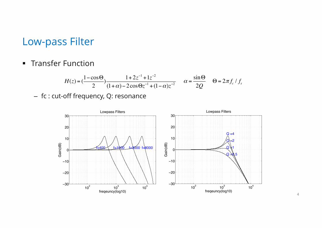
Low-pass Filter

§ Transfer Function

– fc : cut-off frequency, Q: resonance

4

H (z) = (1− cosΘ2

) 1+ 2z−1 +1z−2

(1+α)− 2cosΘz−1 + (1−α)z−2α =

sinΘ2Q

102 103 104−30

−20

−10

0

10

20

30

f=400 f=1000 f=3000 f=8000

Lowpass Filters

freqeuncy(log10)

Gai

n(dB

)

102 103 104−30

−20

−10

0

10

20

30

Q =0.5

Q =1

Q =2

Q =4

Lowpass Filters

freqeuncy(log10)

Gai

n(dB

)

Θ = 2π fc / fs

High-pass Filter

§ Transfer Function

5

H (z) = (1+ cosΘ2

) 1− 2z−1 +1z−2

(1+α)− 2cosΘz−1 + (1−α)z−2α =

sinΘ2Q

Θ = 2π fc / fs

102 103 104−30

−20

−10

0

10

20

30

f=400 f=1000 f=3000 f=8000

Highpass Filters

freqeuncy(log10)

Gai

n(dB

)

102 103 104−30

−20

−10

0

10

20

30

Q =0.5

Q =1

Q =2

Q =4

Highpass Filters

freqeuncy(log10)

Gai

n(dB

)

Band-pass filter

§ Transfer Function

6

H (z) = (sinΘ2) 1− z−2

(1+α)− 2cosΘz−1 + (1−α)z−2

102 103 104−30

−20

−10

0

10

20

30

f=400 f=1000 f=3000 f=8000

Bandpass Filters

freqeuncy(log10)

Gai

n(dB

)

102 103 104−30

−20

−10

0

10

20

30

Q =0.5

Q =1

Q =2

Q =4

Bandpass Filters

freqeuncy(log10)

Gai

n(dB

)

α =sinΘ2Q

Θ = 2π fc / fs

Notch filter

§ Transfer Function

7

H (z) = 1− 2cosΘz−1 + z−2

(1+α)− 2cosΘz−1 + (1−α)z−2α =

sinΘ2Q

Θ = 2π fc / fs

102 103 104−30

−20

−10

0

10

20

30

f=400 f=1000 f=3000 f=8000

Notch Filters

freqeuncy(log10)

Gai

n(dB

)

102 103 104−30

−20

−10

0

10

20

30

Q =0.5

Q =1

Q =2

Q =4

Notch Filters

freqeuncy(log10)

Gai

n(dB

)

102 103 104−30

−20

−10

0

10

20

30

AdB=−12

AdB=−6

AdB=0

AdB=6

AdB=12

EQ

freqeuncy(log10)

Gain(dB)

102 103 104−30

−20

−10

0

10

20

30

AdB=−12

AdB=−6

AdB=0

AdB=6

AdB=12

EQ

freqeuncy(log10)

Gain(dB)

Equalizer

§ Transfer Function

8

H (z) = (1+α ⋅A)− 2cosΘz−1 + (1+α ⋅A)z−2

(1+α / A)− 2cosΘz−1 + (1−α / A)z−2α =

sinΘ2Q

Θ = 2π fc / fs

Q=1 Q=4

References

§ Cookbook formulae for audio EQs based on biquad filter (R. Bristow-Johnson)– http://www.musicdsp.org/files/Audio-EQ-Cookbook.txt

9

Compressor

§ Audio effect unit for automatic gain control – Boost the level for soft signals and suppress it for loud signals– Typically used as a front-end processor in sound recording

§ Signal Processing Pipeline

10

GainCurve

EnvelopDetector

Input

OutputX

Envelope Detector

§ Detecting the level of signal

§ Different sensitivity for increasing (attack) and decreasing (release) levels– During attack:

– During release:

11

Full-waverectificationInput Leaky

Integratorenvelope

y(n) = y(n−1)+ (1− e−1(attack _ time* fs) )( x(n) − y(n−1))

y(n) = y(n−1)+ (1− e−1(release_ time* fs) )( x(n) − y(n−1))

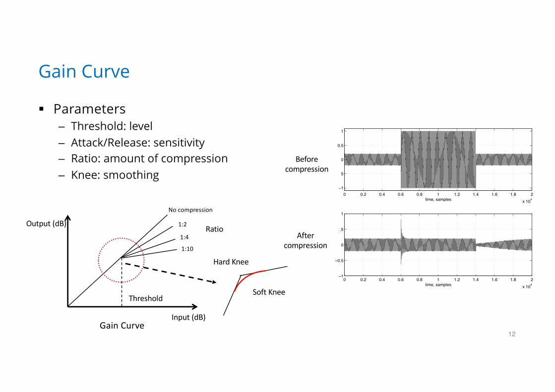
Gain Curve

§ Parameters– Threshold: level– Attack/Release: sensitivity– Ratio: amount of compression– Knee: smoothing

12

Input(dB)

Output(dB)

Threshold

Nocompression

GainCurve

1:2

1:4

1:10

Ratio

SoftKnee

HardKnee

Signal Processing Techniques for Digital Audio Effects 26

Example: Compressor Attack / Release

0 0.2 0.4 0.6 0.8 1 1.2 1.4 1.6 1.8 2x 104

−1

−0.5

0

0.5

1

time, samples

0 0.2 0.4 0.6 0.8 1 1.2 1.4 1.6 1.8 2x 104

−1

−0.5

0

0.5

1

time, samples

Figure 20: Compressor Input and Output.

• this is a limiter, ρ =∞.

• attack is faster than release: τ ≈ 10mS,τr ≈ 100mS.

Beforecompression

Aftercompression

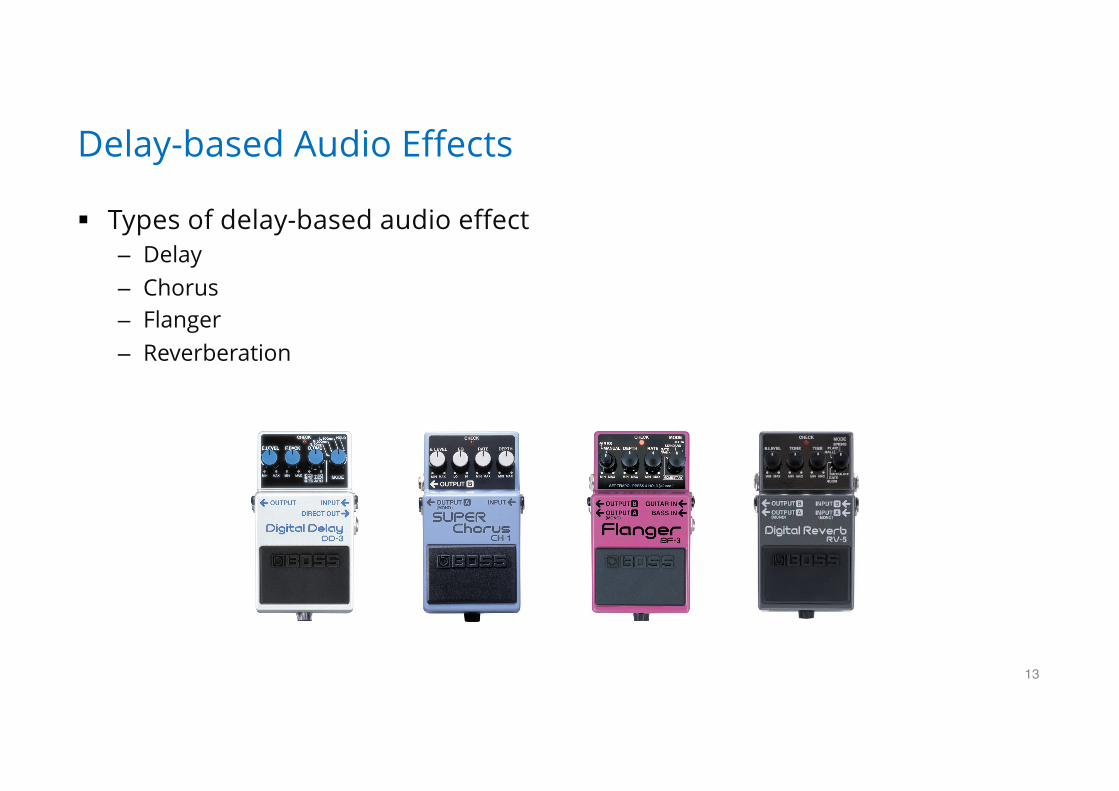
Delay-based Audio Effects

§ Types of delay-based audio effect– Delay– Chorus– Flanger– Reverberation

13

Delay

§ Delay effect– Generate repetitive loop delay– Feedback coefficient controls the amount of delayed input– Can be extended to stereo signals such that the delay output is “ping-ponged”

between the left and right channels– The delay length is often synchronized with music tempo– The delayline is implemented as a “circular buffer”

14

+x(n)

feedback

y(n)Dry

+

Wet

DelayLine

Chorus

§ Chorus effect– Gives the illusion of multiple voices playing in unison– By summing detuned copies of the input– Low frequency oscillators are used to modulate the position of output tops à This

causes the pitch of the input (resampling!)

15

LFOs

x(n)

y(n)Dry

+

+

Wet

DelayLine

Flanger

§ Flanger effect– Originally generated by summing the output of two un-locked tape machines while

varying their sync (used to be called “reel-flanging”)– Emulated by summing one static tap and variable tap in the delay line

• Feed-forward combine filter where harmonic notches vary over frequency.– LFO is often synchronized with music tempo

16

x(n)

+

LFOs

StatictapVariabletap

y(n)+

WetDry

DelayLine

Reverberation

§ Natural acoustic phenomenon that occurs when sound sources are played in a room– Thousands of echoes are generated as sound sources are reflected against wall, ceiling

and floors– Reflected sounds are delayed, attenuated and low-pass filtered: high-frequency

component decay faster– The patterns of myriads of echoes are determined by the volume and geometry of room

and materials on the surfaces

17

SoundSource

ListenerDirectsound

Reflectedsound

Reverberation

§ Room reverberation is characterized by its impulse response (IR)– E.g. when a balloon pop is used as a sound source

§ The room IR is composed of three parts– Direct path– Early reflections – Late-field reverberation: high echo density

§ RT60– The time that it takes the reverberation to decay

by 60 dB from its peak amplitude

18

Signal Processing Techniques for Digital Audio Effects 70

Reverberation and Linear Time-Invariant Systems

0 10 20 30 40 50 60 70 80 90 100-0.4

-0.2

0

0.2

0.4

0.6

0.8

1CCRMA Lobby Impulse Response

time - milliseconds

resp

onse

am

plitu

de

direct path

early reflections

late-field reverberation

Figure 61: CCRMA lobby response to transient signal

• The arrival times and nature of reflected source signals are sen-sitive to the details of the environment geometry and materials.

• As a result, reverberation may seem unmanageably complex.

• Fortunately, reverberation has two properties which allow itsanalysis and synthesis without having to know the details:

– linearity, and

– time invariance.

• Here, we explore reverberation by studying impulse responsesof enclosed spaces.

Artificial Reverberation

§ Mechanical reverb– Use metal plate and spring– Plate reverb: https://www.youtube.com/watch?v=XJ5OFpvX5Vs

§ Delayline-based reverb– Early reflections: feed-forward delayline– Late-field reverb: allpass/comb filter, feedback delay networks (FDN)– “Programmable” reverberation

§ Convolution reverb– Measure the impulse response of a room– Do convolution input with the measured IR

19

Delay-based Reverb

20

Z-M+x(n)

_

+ y(n)

AllPass filter/Combfilter(whenonetapisabsent)

- Thelengthsofdelaylinesarechosensuchthattheirgreatestcommonfactorsissmall(e.g.primenumbers)

- Themixingmatrixischosentobeunitary(orthonormal)

+x(n)

FeedbackDelayNetworks

Z-M1

Z-M2

Z-M3+

a11a12a13a11a12a13a11a12a13

y(n)

- AreverbisconstructedbycascadingmultipleAPorFFCFunits

Convolution Reverb

§ Measuring impulse responses

– If the input is a unit impulse, SNR is low– Instead, we use specially designed input signals

• Golay code, allpass chirp or sine sweep: their magnitude responses are all flat but the signals are spread over time

– The impulse response is obtained using its inverse signal or inverse discrete Fourier transform

21

Signal Processing Techniques for Digital Audio Effects 74

Impulse Response MeasurementMeasurement Model:

Figure 63: Measurement Configuration

- Room presumed LTI.- Why not just crank an impulse out the speaker, record the resultand declare victory?

s(t)

LTI system

r(t)

test sequence

measured response

n(t)

h(t)

measurement noise

Figure 64: Measurement Model

- Noise assumed additive, unrelated to the test signal. (How will itbe related to the system?)

Signal Processing Techniques for Digital Audio Effects 75

Measurement Approach:- Given the measurement model

r(t) = s(t) ∗ h(t) + n(t),

the idea is to find a test signal which will reveal the impulse responseh(t).- Put an impulse into the room,

s(t) = δ(t),

and estimate h(t) as the system response,

h(t) = r(t).

- How good is this estimate h(t)?

0 5 10 15 20 25 30 35 40 45 50-0.4

-0.2

0

0.2

0.4

0.6

0.8Example Measured Impulse Response

time - milliseconds

resp

onse

am

plitu

de

Figure 65: Measured Impulse Response

Convolution Reverb

22

Music 318, Winter 2007, Impulse Response Measurement 13

0 500 1000 1500-0.5

0

0.5sine sweep, s(t)

ampl

itude

frequ

ency

- kH

z

sine sweep spectrogram

0 200 400 600 800 10000

5

10

0 500 1000 1500 2000-1

-0.5

0

0.5

1sine sweep response, r(t)

time - milliseconds

ampl

itude

time - milliseconds

frequ

ency

- kH

z

sine sweep response spectrogram

0 500 1000 1500 20000

5

10

0 100 200 300 400 500 600 700 800 900 1000-0.04

-0.02

0

0.02

0.04

0.06

0.08measured impulse response

time - milliseconds

ampl

itude

CCRMA Lobby Measurment Example

s(t)

r(t)

ˆ h (t)

(J.Abel)

Spatial Hearing

§ A sound source arrives in the ears of a listener with differences in time and level– The differences are the main cues to identify where the source is.– We call them ITD (Inter-aural Time Difference) and IID (Inter-aural Intensity Difference)– ITD and IID are a function of the arrival angle.

23

R

L

ITD

IID

Head-Related Transfer Function (HRTF)

§ A filter measured as the frequency response that characterizes how a sound source arrives in the outer end of ear canal– Determined by the refection on head, pinnae or other body parts– Function of azimuth (horizontal angle) and elevation (vertical angle)

24

𝐻"(𝜔, ∅, 𝜃)

𝐻)(𝜔, ∅, 𝜃)

R

L

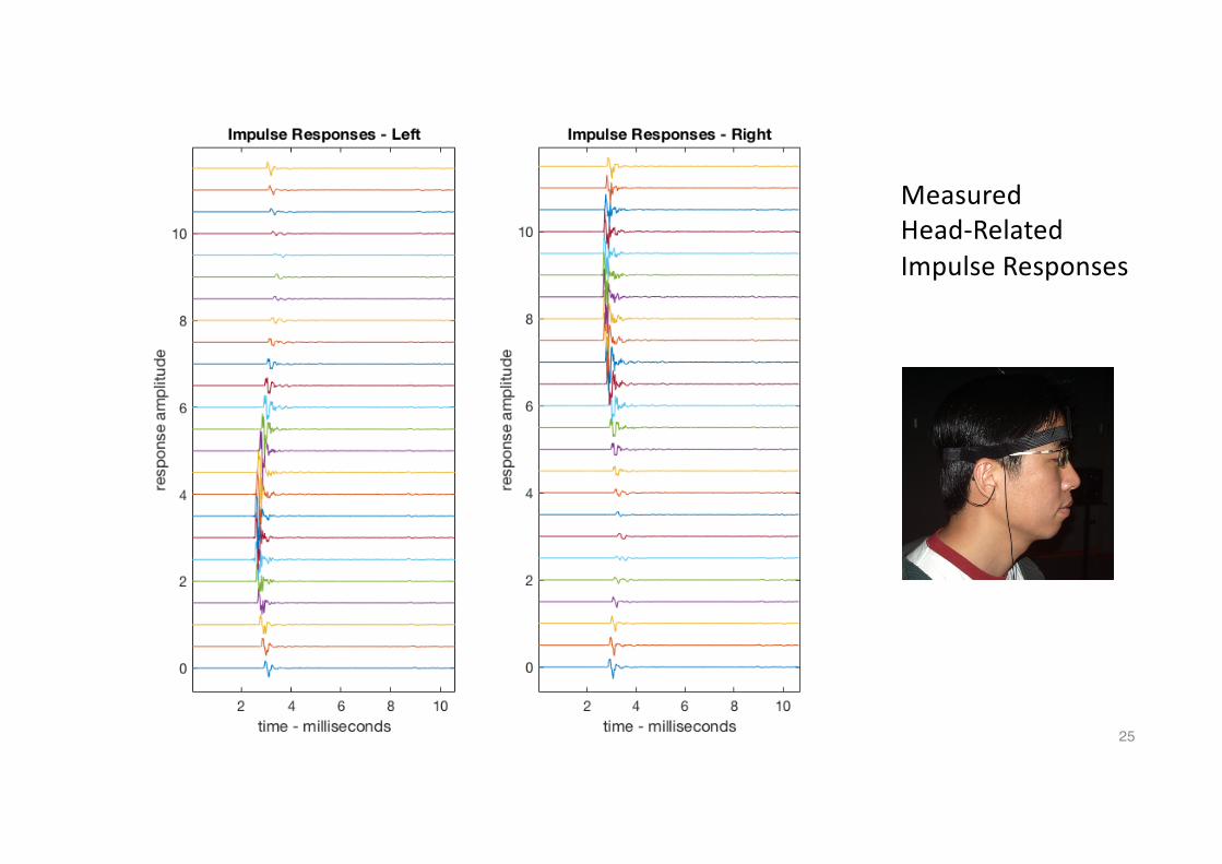
25

Fall 2007 Music 220D Report Kolar 3

Subject/Receiver Alignment: subject wearing mic attachment/strain relief and mirror-

alignment headgear positioned on rotating stool (noted during 2nd

session that midpoint of

rotation not fixed because of seat asymmetry); flashlight suspended above subject to

reflect light off top-of-head mirror onto azimuth markings on walls for sighted alignment

by subject (fig. 3); line-of-sight verification by subject for speaker elevation alignment

figure 3: receiver mic attachment & alignment headgear, flashlight-mirror-marker positioning system

Equipment/Signal Chain: AuSIM HeadZap speaker (fig. 2 & 3) powered by Samson

Servo 120 amplifier, AuSIM Binaural Probe Microphone Set (AuPMC002, Sennheiser

KE4-211-2 omni electret capsules, fig. 4) into Grace 101 preamplifier, RME Fireface 800

converter, Digital Performer 5.12 recording software on MacBook Pro running OS

10.4.11.

figure 3: AuSIM Binaural Probe Microphone specifications and response per product literature

MeasuredHead-RelatedImpulseResponses

26

MagnituderesponseoftheHRIRs

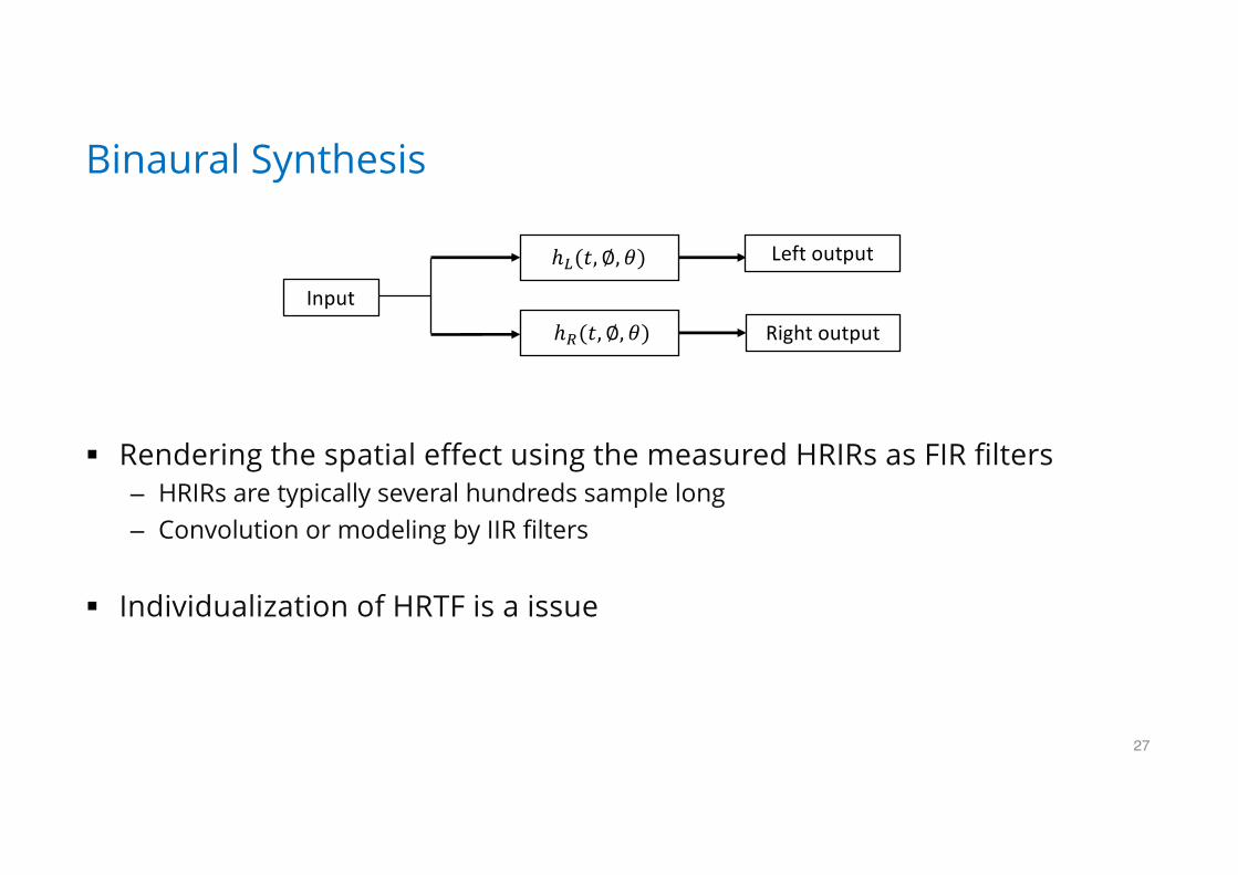
Binaural Synthesis

§ Rendering the spatial effect using the measured HRIRs as FIR filters– HRIRs are typically several hundreds sample long – Convolution or modeling by IIR filters

§ Individualization of HRTF is a issue

27

Input

Leftoutput

Rightoutput

ℎ"(𝑡, ∅, 𝜃)

ℎ)(𝑡, ∅, 𝜃)

Playback Rate Conversion

§ Adjusting playback rate given the sampling rate– Analogy to sliding tapes on the magnetic header in a variable speed– Speeding down: “monster-like”– Speeding up: “chipmunk-like”

28

Playback Rate Conversion

§ Change pitch, length and timbre

29[TheDaFX book]

Resampling

§ Playback rate conversion is performed by resampling– Interpolation on discrete samples– Convolution with interpolation filters– Need to avoid aliasing for down sampling

• Narrowing the bandwidth of the lowpass filter

§ Two Types– Down-sampling: pitch goes up and time shrinks– Up-sampling: pitch goes down and time expands

30

Interpolation Filters

31

−5 −4 −3 −2 −1 0 1 2 3 4 5

0

0.5

1

1.5

Windowed Sinc

Sample Time−5 −4 −3 −2 −1 0 1 2 3 4 5

0

0.5

1

1.5

Linear

Sample Time

−5 −4 −3 −2 −1 0 1 2 3 4 5

0

0.5

1

1.5

3rd−order B−spline

Sample Time−5 −4 −3 −2 −1 0 1 2 3 4 5

0

0.5

1

1.5

3rd−order Lagrange

Sample Time

h(t) =w(t)sinc(t) =w(t) sin(π t)π t

x(d) = x(k)k=−(L−1)

k=L

∑ h(d − k)

Delayedbyd (0<d <1)