Embed Size (px)
Citation preview

CTIOPI Photometry Reduction User Guide
Wei-Chun Jao
Georgia State University
04/13/2003

– 2 –
Revision History
1. 04/20/03 by Wei-Chun Jao — Remarks section added.
2. 08/05/03 by Wei-Chun Jao — New evalfit.pl script released to match
CTIOPI/SMARTS photometry catalogue.
3. 08/07/03 by John Subasavage — Cosmic ray section added, grammar corrections.
4. 08/28/03 by Wei-Chun Jao — New standard.pl script released.
5. 04/17/08 by Jen Winters — Fixairmass and setairmass tasks added, grammar
corrections.
6. 05/09/12 by Jen Winters — Clarification, reorganizing, grammar corrections.
7. 04/26/13 by John Lurie — Revised aperture sizes for aperture correction.
Also, RMS < 0.02 for fitparams (Section 3.7).

– 3 –
1. Before Starting
Before starting to reduce photometry, you might need to know a little background
on photometry (ie, extinction, airmass, transformation equation, et. al.). Astronomical
Photometry written by Henden, A. and Kaitchuck, R. is a good introductory
book for those who want to get a first look at photometry. Users should also be
familiar with IRAF. A couple of user guides can be found on IRAF’s website –
http://iraf.noao.edu/docs/photom.html, specifically
1. A User’s Guide to Stellar CCD Photometry with IRAF
2. A User’s Guide to CCD Reductions with IRAF
This manual will skip these introductory parts and start with the processed data.
Please read the Parallax Reduction Guide to learn how to process the raw data for
CTIO or see Astrometry: Slurping Data from CTIO on the RECONS Data Reduction
page.
Have all the finder charts, observing log (if available) and airmass table (a bird’s eye
view of all the objects obseved in that night) ready.
2. Oragnize Your Processed Data
Load packages daophot, photcal, redpi before you begin anything1. After processing
the raw data, you will need to fix the airmass immediately. The new TCS does not
1Patterson, R. J. et al (1998) shows that no significant difference was found between
IRAF/APPHOT and IRAF/DAOPHOT, although APPHOT is claimed for aperture
photometry

– 4 –
communicate effectively with the telescope, and thus, the airmass is not accurate. This
package will correct the airmass. Run files *.o.fits >> listfile in IRAF. You will also need
to create a file called “coords” that contains the coordinates for each object. You can get
these from the most recent photometry observing list posted on the protected page. The
format for this file is as follows (note that you need the colons and only one space between
the RA and DEC):
11:56:06.1 −48:39:46.0
Make sure that “listfile” and “coords” have the same number of lines or else it will
crash. Then, run fixairmass
Next, you will need to fix the headers. Load the astutil task. See Fig 1. Edit
setairmass parameters for the correct observatory site. Run this task to calculate the
airmass at the middle of the exposure. A new header keyword, utmiddle, will be added
in the header. If any of the following headers are missing, date-obs, RA, ST, epoch or
airmass, this setairmass won’t work. You will need to add those header-keywords back to
the header by using the hedit task.
Sort this data into two directories, standard and science.
Run files *.o.fits >> listfile in IRAF in both the standard and science directories.
Then, run displayexam task to examine the the images and note if any stars are saturated.
This step is important for data reduction, as photometry of saturated stars cannot be
determined. Furthermore, IRAF won’t generate the annoying “INDEF” in the data file.
In the meantime, you can determine the average seeing (FWHM) for this night’s data.
This average FHWM will be entered in the phot task. Because the science star images
are sandwiched between the standard star frames, you can simply apply the FWHM of the
standard stars to the science stars. If the oberving log is available, you may select those
good frames and the average seeing based on those recorded in log book. For example, if

– 5 –
a field was observed in V, R and I, choose the best one in the I-band in order to reduce
potential output problems from IRAF. Otherwise, the same V and R images will need to
be used twice to make two sets of VRI. If a field is observed in V, V, R, R, I and I, two sets
of VRI can be chosen so that you will have two sets of photometry results calculated from
IRAF. One additional step is to determine which stars will need an aperture correction.
This is a good time to make a note of whether each frame can use the standard 7′′ radius
aperture and if not, what the maximum aperture is without contamination. Standards
rarely need an aperture correction; however, science stars are often in crowded fields and
require a correction.
3. Standard Stars
The basic steps for reducing uncrowded standard star fields are
1. Determine the FWHM and remove cosmic rays.
2. Determine the aperture size you wish to use. This aperture size will be applied to
all the standard stars from all the nights for all the filters. Edit the datapars,
centerpars, fitskypars and photpars task parameters in the phot task.
3. Use the redpi/apercorr task to tag the standard stars so that the instrumental
magnitudes can be calculated.
4. Organize the standard star configuration file and collect your standard stars’ VRI
instrumental magnitudes.
5. Apply transformation equations to get the apparent magnitudes for the standard
stars.
– 6 –
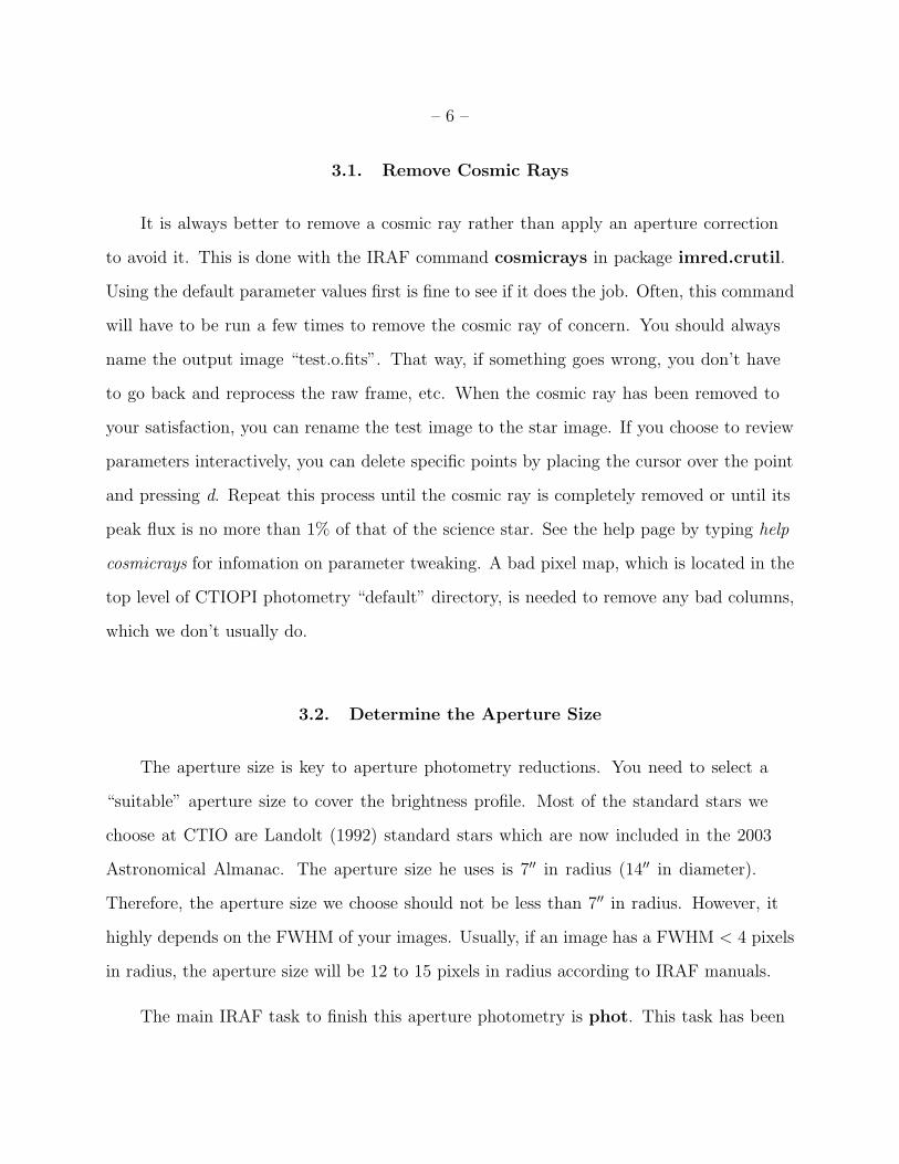
3.1. Remove Cosmic Rays
It is always better to remove a cosmic ray rather than apply an aperture correction
to avoid it. This is done with the IRAF command cosmicrays in package imred.crutil.
Using the default parameter values first is fine to see if it does the job. Often, this command
will have to be run a few times to remove the cosmic ray of concern. You should always
name the output image “test.o.fits”. That way, if something goes wrong, you don’t have
to go back and reprocess the raw frame, etc. When the cosmic ray has been removed to
your satisfaction, you can rename the test image to the star image. If you choose to review
parameters interactively, you can delete specific points by placing the cursor over the point
and pressing d. Repeat this process until the cosmic ray is completely removed or until its
peak flux is no more than 1% of that of the science star. See the help page by typing help
cosmicrays for infomation on parameter tweaking. A bad pixel map, which is located in the
top level of CTIOPI photometry “default” directory, is needed to remove any bad columns,
which we don’t usually do.
3.2. Determine the Aperture Size
The aperture size is key to aperture photometry reductions. You need to select a
“suitable” aperture size to cover the brightness profile. Most of the standard stars we
choose at CTIO are Landolt (1992) standard stars which are now included in the 2003
Astronomical Almanac. The aperture size he uses is 7′′ in radius (14′′ in diameter).
Therefore, the aperture size we choose should not be less than 7′′ in radius. However, it
highly depends on the FWHM of your images. Usually, if an image has a FWHM < 4 pixels
in radius, the aperture size will be 12 to 15 pixels in radius according to IRAF manuals.
The main IRAF task to finish this aperture photometry is phot. This task has been

– 7 –
included in redpi/apercorr option 3 task. phot is a task with other tasks – datapars,
centerpars, fitskypars and photpars – nestled inside.
3.3. Modify Parameters in PHOT Task
When you load the redpi/apercorr task, there will be 4 options. Select option 4 for
standard stars because standard stars are usually in uncrowded fields where no aperture
correction necessary, unless some bonehead has positioned a star too close to the bad
column. After choosing option 4, you will need to modify the following parameters in each
task by scrolling down (using the up and down arrow keys) to each and typing :e.
3.3.1. photpars
This task specifies the size of the aperture. It is 7′′ in radius in Fig 1. If mkapert is set
to “yes”, it will indicate the aperture size on the radial plot while you tag the stars. This is
helpful to see whether any contamination will fall within the aperture.
3.3.2. datapar
Fig 2 shows the parameter examples for this task. The key parameter is fwhmpsf
because it will be different from night to night. Average the FWHM for all the standard
star images. If we specify the scale of the CTIO 0.9m data (i.e. the plate scale) to be
0.401′′, then multiplying the FWHM by the scale will give us the FWHM in arcseconds.
Other parameters are a one-time setup.

– 8 –
3.3.3. centerpar
This task will determine the centering algorithm while we tag the stars. Therefore, the
calgorithm will be “centroid” as shown in Fig 2. The other parameter needing modification
from image to image is cbox. Usually it is two times of the fwhmpsf. The unit here is still
in arcseconds.
3.3.4. fitskypars
The background noise will affect the quality of aperture photometry. You will need to
select the size of the sky and sky annulus to calculate the background noise. Currently, we
choose a radius of 20′′ with a 3′′ annulus width as shown in Fig 2. If mksky is set to “yes”,
it will indicate the sky annulus on the radial plot.
After you modify all these parameters, the apercorr task will automatically display
every image within the listfile so you can move the cursor onto the image to tag the stars
you need using the spacebar. A radial plot will be shown and will mark the aperture and
sky annulus size. A new file *.mag.1 will be generated after you click q to quit the tagging
sequence. Please make sure that the tagging order of the images is the same in each filter.
3.4. Make Observation Files
The instrumental magnitude for each standard star has been calculated and listed
within each *.mag.1 file. Before assembling them into a master file, you need to use
the mkimsets task to sort these images. See Fig 3. The output file should be named
“standard.imsets”, which stands for “standard fields image sets”. The first column indicates
the ID of each standard field, the second, third and fourth column are V, R, and I filters,

– 9 –
respectively. You can see that the standard field 1 was observed one time in the V and R
filters, but two times in the I filter (1004 and 1005) in Fig 3. Standard field 2 was observed
two times in each.
3.5. Make Master List of Instrumental Magnitudes
The next step will be to extract all the instrumental magnitudes in *.mag.1 into
a master file. The task to be used is mknobsfile, as shown in Fig 3. The output
file “standard.obs” is the master list. If there are three stars in standard field 1, this
“standard.obs” file will label these stars in sequential order, 1, 2 and 3. After it finishes,
please open this output file to check the filter orders, because this task sometimes will have
problems. If an aperture correction was applied, be sure to include that filename (usually
aperture.corr) under the apercors parameter.
3.6. Make Configuration File and Standard VRI Magnitude Table
An example configuration file is shown in Fig 4 that defines the transformation
equation for the photometry. More detail on this equation is in section 5. All of the “.cfg”
files for standard and science stars are found in the directory named “default” in the top
directory on the photometry disk. The standard star magnitude table needs to be created,
and an example is shown in Fig 3. All standard stars you use need to be included in
“landvri.dat” file. The stars’ IDs in “landvri.dat” should be identical with those
in “standard.obs”.

– 10 –
3.7. Final Steps for Standard Stars
The last task to use in this standard star data processing is fitparams, shown in
Fig 5. Basically, the task will apply the method of least-squares to the transformation
equation to calculate apparent magnitudes for the standard stars and also to determine
the transformation equation coefficients (standard.coeff) so that we can apply those
coefficients to our science stars. We force the RMS to be less than 0.02, so pay attention to
that.
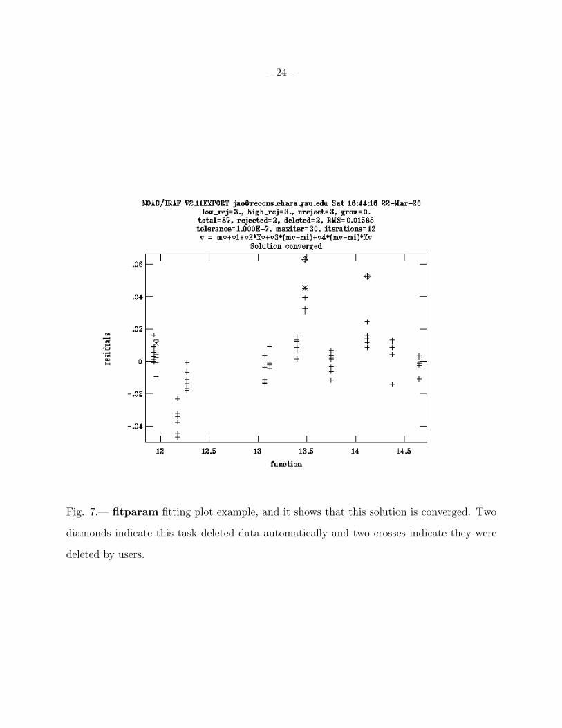
This task will plot a residual and also tell you if the solution converges or not. If it
does not converge in one filter, you may need to delete a couple of high residual stars and
then fit again (shown in Fig 7). Please read the help manual of fitparam task for more
details. You may quit this task after these three fittings converge. If the solution converges
the first time, there will be three main blocks in the standard.coeff file. If not, some extra
blocks with “diverge” will be noted in this file. The last three blocks in this file indicate the
final coefficient results for this transformation.
In order to generate a master photometry list for CTIOPI, a perl script has to be
run: perl ∼/bin/standard.pl. The input files are “standard.imsets” and “standard.obs”.
Please modify the “standard.imsets” file. First, remove the first two blank lines. Second,
make one line for each object. A file “standard.catalog” as shown in Figure 6 is
generated after running this script. THIS SCRIPT WILL NOT CALCULATE THE
EXTINCTION CURVE. IT GENERATES THE CATALOGUE ONLY.
FURTHERMORE, PLEASE MANUALLY ADD THOSE USELESS
IMAGES (ex: bad images, saturated images) BACK TO THIS CATALOGUE
FILE.
Now you have finished processing the standard stars and have gotten the transformation
– 11 –
coefficients. Next, continue to work on the science stars.
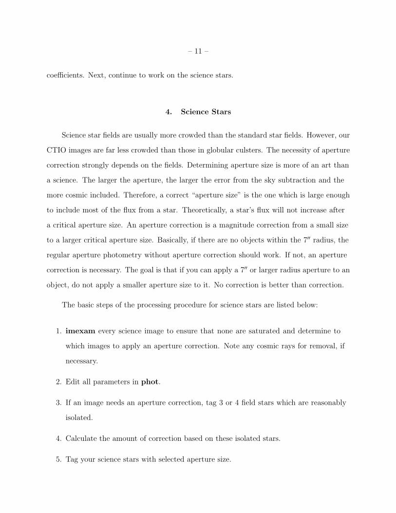
4. Science Stars
Science star fields are usually more crowded than the standard star fields. However, our
CTIO images are far less crowded than those in globular culsters. The necessity of aperture
correction strongly depends on the fields. Determining aperture size is more of an art than
a science. The larger the aperture, the larger the error from the sky subtraction and the
more cosmic included. Therefore, a correct “aperture size” is the one which is large enough
to include most of the flux from a star. Theoretically, a star’s flux will not increase after
a critical aperture size. An aperture correction is a magnitude correction from a small size
to a larger critical aperture size. Basically, if there are no objects within the 7′′ radius, the
regular aperture photometry without aperture correction should work. If not, an aperture
correction is necessary. The goal is that if you can apply a 7′′ or larger radius aperture to an
object, do not apply a smaller aperture size to it. No correction is better than correction.
The basic steps of the processing procedure for science stars are listed below:
1. imexam every science image to ensure that none are saturated and determine to
which images to apply an aperture correction. Note any cosmic rays for removal, if
necessary.
2. Edit all parameters in phot.
3. If an image needs an aperture correction, tag 3 or 4 field stars which are reasonably
isolated.
4. Calculate the amount of correction based on these isolated stars.
5. Tag your science stars with selected aperture size.

– 12 –
6. Generate the science star configuration file and collect your science stars’ VRI
instrumental magnitudes.
7. Based on the transformation equation coefficients from standard stars, calculate
apparent magnitudes.
4.1. Examine Science Images
Understanding the quality of your science images is important because you need to
apply the right method to process your precious data. Run the redpi/displayexam to
examine all the science images. Meanwhile, determine the necessity of aperture correction
for science stars and make a note of which images have cosmic rays within a 7′′ radius of
the science star.
4.2. Making an Aperture Correction
Sometimes no aperture correction is needed on any science star in a night of photometry.
If that is the case, shout “Hooray” and skip to the section Get Instrumental Magnitudes
for Science Stars. However, we are not usually that lucky, so if you do need to make an
aperture correction, continue on to the next section.
4.2.1. Tag Isolated Stars in a Crowded Field
Load redpi/apercorr task and choose option 1. It will allow you to edit the
parameters of the phot task. Section 3.3 has explained these parameters. The most
important task is photpars. You need to choose a large variety of aperture sizes: 2′′, 2.5′′,
3′′, 3.5′′, 4′′, 4.5′′, 5′′, 5.5′′, 6′′, 6.5′′, and 7′′ in radius. Then you tag 3 or more “isolated”

– 13 –
stars with reasonable counts in the same field. These stars do not need to be tagged in the
same order or even be the same stars in each filter, but you must tag the same number of
stars in each filter. The new generated file is called *.aper.1.
4.2.2. Apply Aperture Correction
Option 2 in redpi/apercorr will do this work. The actual task behind the curtain is
mkapfile shown in Fig5. A curve of growth, which is a plot of magnitude within a given
aperture versus aperture size, will be shown for each image with *.aper.1.
index 1 2 3 4 5 6 7 8 9 10 11
radius size 2 2.5 3 3.5 4 4.5 5 5.5 6 6.5 7
The parameter naperts is the total number of apertures you want to extract. In the
example above, there are fourteen different sizes. smallap indicates the small aperture
index you would like to apply on the science stars. largeap indicates the large aperture
size index which you would like to correct to. In the example shown in Fig 5, the smallap
ID should be 7 (5′′ radius) and the largeap ID should be 11 (7′′ radius). The output file
for this mkapfile is called aperture.corr.
This file is a simple text file containing the image name in column 1, the aperture
correction computed from smallap to largeap in column 2, and the estimated error in the
aperture correction in column 3. If multiple aperture sizes were used on one night, create
a 4th column and enter the aperture radius in arcseconds for each image. A # needs to
preceed this column so that it does not affect the calculation to come later. For example:
20030101.09.101.o -0.01218093 8.684811E-4 #5′′
20030101.09.112.o -0.08370557 0.004138806 #1′′

– 14 –
4.3. Get Instrumental Magnitudes for Science Stars
This step is similiar to the standard star tagging procedure. The task you need to load
is redpi/apercorr option 3. This option will let you edit phot parameters. The only
important parameter you need to notice is apertures. The correct aperture size is the
same as the smallap (in units of arcseconds) which you used in the aperture correction.
If no aperture correction was needed, this is just the (7′′ radius) that you used when you
tagged the standard stars. Again, when tagging science stars, the tagging order should
be the same for all filters, i.e., those cases where photometry for both components of a
widely separated binary system is possible. The output file is called *.mag.1.
4.4. make science star observation files and master list files
The mkimsets task is used for science stars just as for standard stars. The output file
is “science.imsets”. After this file is generated, please make sure the top two blank lines
are removed. Use mknobsfile to generate a master list of instrumental magnitudes. Make
the necessary changes for this task: apercors=“aperture.corr” if an aperture correction
was done, imsets=“science.imsets”, and observation=“science.obs”. If no aperture
correction was done, then the apercors line in the mknobsfile task should be blank.
4.5. Calculate Apparent Magnitude
There are two ways to calculate the apparent magnitude. One is with evalfit, an IRAF
standard task, and the other is with evalfit.pl which is a perl script. The latter produces
an output consistent with the CTIOPI photometry catalogue and is preferred.

– 15 –
4.5.1. evalfit task
Before using this task, you need to copy the “standard.coeff” file from the standard
star directory. No modification to this file is necessary. The other two files you need to
use in this task are “science.cfg” which is the same as “standard.cfg”, and “science.obs”.
Therefore, science and standard stars will have the same transformation equation. An
example parameter for evalfit is shown in Fig 5.
The output file is called “evalfit.out”. The S/N magnitude error is also printed in this
file. More discussion about error can be found in section 5.
4.5.2. perl script
This perl scrip is called evalfit.pl. Have a copy of it under your bin directory, because
the date/format perl module is called, logon penston. Type perl ∼/bin/evalfit.pl to
excute it. This perl script is only applied for a second-order transformation equation as
shown in section 5. The “standard.coeff” and “science.obs” files are also necessary for this
script. However, you need to modify this file by leaving the last block of converged VRI
results in this file. No divergent result can exist in this file.
The default name for the file created by mkimsets needs to be “science.imsets” for
this script. Also in the case where a series of frames were taken of a double star, you need
to insert an extra line for the second star which has the same frame name as the first star.
For example,
LHS300AB : 20030101.09.101.o 20030101.09.102.o 20030101.09.103.o
should be modified to look as follows:
LHS300A : 20030101.09.101.o 20030101.09.102.o 20030101.09.103.o
LHS300B : 20030101.09.101.o 20030101.09.102.o 20030101.09.103.o

– 16 –
The output file “science.ans” is shown in Fig 6. This file includes the standard star
error as well as other important parameters such as airmass. More discussion about
magnitude error can be found in section 5. This file needs to be manually edited to include
the diameter of the aperture size used. For example, if you used the standard 7′′ radius,
you will enter 14′′ for that image.
As discussed in the standard star section, PLEASE MANAULLY ADD THOSE
USELESS IMAGES (ex: bad images, saturated images) BACK TO THIS
CATALOGUE FILE.
5. Transformation Equations
The transformation equations for aparent magnitude V(RI)c are as follows,
V = mV + a1 + a2X + a3(mV − mI) + a4(mV − mI)X (1)
R = mR + b1 + b2X + b3(mR − mI) + b4(mR − mI)X (2)
I = mI + c1 + c2X + c3(mR − mI) + c4(mR − mI)X (3)
where, V,R and I are the aparent magnitudes for standard stars, mV RI is the
instrutmental magnitude from IRAF, a1 to a4 are the transformation coefficients (same for
bi and ci), and X is the airmass.
The method of least-squares is performed by the fitparam task to calculate the
transformation coefficients based on the standard star observations. This task calculates
not only the transformation coefficients but also the so-called “external error” or “standard
star error”. This standard deviation error can be found in the fitparam output “logfile”.
Another magnitude error is the “internal error” or “night-to-night error”, which is the
error from the repeated observation of the same object. The smallest error is called the

– 17 –
“photon error” which indicates the signal-to-noise ratio received by the detector. This error
is printed in the output file of the evalfit IRAF task. Because of the large signal-to-noise
ratio, this error is usually very small.
6. Remarks About Sky Subtraction
When subtracting the sky background, you must choose an inner radius for
the sky annulus and a width for the annulus. The example given here uses the
noao.digiphot.daophot.phot task applied to the standard star field SA98. The seeing on
that night (14 NOV 2001) was 1.4′′, or 3.5 pixels. The parameter file for the task fitskypars
is shown in Fig 2 (the numbers entered for the parameters “annulus” and “dannulus” are
in arcseconds). Mean sky counts for two example inner radii for the sky annulus (10′′ and
20′′) are shown in Table 1. In both cases the width is 3′′.
star 10′′(radius) 20′′(radius) note
SA98−650 58.33632 57.91608
SA98−670 63.51149 58.55741
SA98−676 60.38068 58.39950 mix with SA98−675
SA98−675 61.22947 58.12084 mix with SA98−676
Two things can be seen in these results: (1) the 20′′ inner annulus radius has lower
counts (and lower standard deviations, not shown) than the 10′′ radius — the smaller radius
may include counts from the wings of the star, indicating that a larger sky annulus radius
is preferred, and (2) even when a nearby star is within the sky annulus width, e.g. SA−676
and SA98−675, the mean sky counts are not affected.

– 18 –
−−−−−−−−−−−−−setairmass−−−−−−−−−−−−− images = "@listfile" Input images (observatory = "CTIO") Observatory for images (intype = "beginning") Input keyword time stamp (outtype = "effective") Output airmass time stamp\n (date = "date−obs") Observation date keyword (exposure = "exptime") Exposure time keyword (seconds) (airmass = "airmass") Airmass keyword (output) (utmiddle = "utmiddle") Mid−observation UT keyword (output)\n (show = yes) Print the airmasses and mid−UT? (update = yes) Update the image header? (override = yes) Override previous assignments? (mode = "ql")
−−−−−−−−−−−−task=phot−−−−−−−−−−−− image = "" Input image(s) coords = "" Input coordinate list(s) (default: image.coo.?) output = " " Output photometry file(s) (default: image skyfile = "" Input sky value file(s) (plotfile = "") Output plot metacode file (datapars = "") Data dependent parameters (centerpars = "") Centering parameters (fitskypars = "") Sky fitting parameters (photpars = "") Photometry parameters (interactive = yes) Interactive mode ? (radplots = yes) Plot the radial profiles? (verify = )_.verify) Verify critical phot parameters ? (update = )_.update) Update critical phot parameters ? (verbose = )_.verbose) Print phot messages ? (graphics = )_.graphics) Graphics device (display = )_.display) Display device (icommands = "") Image cursor: [x y wcs] key [cmd] (gcommands = "") Graphics cursor: [x y wcs] key [cmd] (mode = "ql")
−−−−−−−−−−−photpars−−−−−−−−−−−(weighting = "constant") Photometric weighting scheme (apertures = "7") List of aperture radii in scale units (zmag = 25.) Zero point of magnitude scale (mkapert = yes) Draw apertures on the display (mode = "ql")
Fig. 1.— parameter examples for setairmass, phot and photpars.

– 19 –
−−−−−−−−−−−datapars−−−−−−−−−−−
(scale = 0.401) Image scale in units per pixel (fwhmpsf = 1.3) FWHM of the PSF in scale units (emission = yes) Features are positive ? (sigma = 5.) Standard deviation of background in counts (datamin = −4.) Minimum good data value (datamax = 65535.) Maximum good data value (noise = "poisson") Noise model (ccdread = "gtron21") CCD readout noise image header keyword (gain = "gtgain21") CCD gain image header keyword (readnoise = 4.7) CCD readout noise in electrons (epadu = 3.1) Gain in electrons per count (exposure = "exptime") Exposure time image header keyword (airmass = "airmass") Airmass image header keyword (filter = "filter2") Filter image header keyword (obstime = "utmiddle") Time of observation image header keyword (itime = 20.) Exposure time (xairmass = 1.2660490274429) Airmass (ifilter = "diar") Filter (otime = "4:50:29.7") Time of observation (mode = "ql")
−−−−−−−−−−−−−centerpars−−−−−−−−−−−−− (calgorithm = "centroid") Centering algorithm (cbox = 2.6) Centering box width in scale units (cthreshold = 0.) Centering threshold in sigma above background (minsnratio = 1.) Minimum signal−to−noise ratio for centering alg (cmaxiter = 10) Maximum iterations for centering algorithm (maxshift = 4.) Maximum center shift in scale units (clean = no) Symmetry clean before centering (rclean = 1.) Cleaning radius in scale units (rclip = 2.) Clipping radius in scale units (kclean = 3.) K−sigma rejection criterion in skysigma (mkcenter = no) Mark the computed center (mode = "ql")
−−−−−−−−−−−−−fitskypars−−−−−−−−−−−−− (salgorithm = "mode") Sky fitting algorithm (annulus = 20.) Inner radius of sky annulus in scale units (dannulus = 3.) Width of sky annulus in scale units (skyvalue = 0.) User sky value (smaxiter = 10) Maximum number of sky fitting iterations (sloclip = 0.) Lower clipping factor in percent (shiclip = 0.) Upper clipping factor in percent (snreject = 50) Maximum number of sky fitting rejection iterati (sloreject = 3.) Lower K−sigma rejection limit in sky sigma (shireject = 3.) Upper K−sigma rejection limit in sky sigma (khist = 3.) Half width of histogram in sky sigma (binsize = 0.10000000149012) Binsize of histogram in sky sigma (smooth = no) Boxcar smooth the histogram (rgrow = 0.) Region growing radius in scale units (mksky = yes) Mark sky annuli on the display (mode = "ql")
Fig. 2.— parameter examples for datapars, centerpars and fitskypars.

– 20 –
−−−−−−−−−−−mkimsets−−−−−−−−−−−
imlist = "*.o.mag.1" The input image list idfilters = "v,r,i" The list of filter ids imsets = "standard.imsets" The output image set file (imobsparams = "") The output image observing parameters file (input = "photfiles") The source of the input image list (filter = ) The filter keyword (fields = "") Additional image list fields (sort = "") The image list field to be sorted on (edit = yes) Edit the input image list before grouping (rename = yes) Prompt the user for image set names (review = yes) Review the image set file with the editor (list = "") (mode = "ql") −−−−−−−−−−−−−−−−−−−−−−−−standard.imsets example:−−−−−−−−−−−−−−−−−−−−−−−−
field1 : dec02s.1001.o dec02s.1003.o dec02s.1004.ofield1 : dec02s.1001.o dec02s.1003.o dec02s.1005.ofield2 : dec02s.1009.o dec02s.1011.o dec02s.1010.ofield2 : dec02s.1012.o dec02s.1013.o dec02s.1014.o
−−−−−−−−−−−−−mknobsfile−−−−−−−−−−−−−
photfiles = "*.o.mag.1" The input list of APPHOT/DAOPHOT databases idfilters = "v,r,i" The list of filter ids imsets = "standard.imsets" The input image set file observations = "standard.obs" The output observations file (obsparams = "") The input observing parameters file (obscolumns = " ") The format of obsparams (minmagerr = 0.001) The minimum error magnitude (shifts = "") The input x and y coordinate shifts file (apercors = "") The input aperture corrections file (aperture = 1) The aperture number of the extracted magnitude (tolerance = 5.) The tolerance in pixels for position matching (allfilters = no) Output only objects matched in all filters (verify = yes) Verify interactive user input ? (verbose = yes) Print status, warning and error messages ? (mode = "ql")
−−−−−−−−−−−−−−−−−−−−−standard.obs example:−−−−−−−−−−−−−−−−−−−−−
field1−1 v 5:59:25.5 1.512 607.395 749.645 16.147 0.001* r 6:01:47.8 1.526 607.467 748.719 14.937 0.001* i 6:03:35.7 1.537 609.185 748.972 14.170 0.001field1−2 v 5:59:25.5 1.512 543.660 558.728 17.673 0.003* r 6:01:47.8 1.526 543.682 557.738 17.036 0.003* i 6:03:35.7 1.537 545.469 558.193 17.288 0.005field1−3 v 5:59:25.5 1.512 967.006 226.776 16.597 0.001* r 6:01:47.8 1.526 967.282 225.602 16.247 0.002* i 6:03:35.7 1.537 968.751 226.254 16.706 0.003
−−−−−−−−−−−−−−−−−−−−−−−−−−−example file of landvri.dat−−−−−−−−−−−−−−−−−−−−−−−−−−−
field1−1 10:54:05.0 −00:50:15.0 8.754 8.240 7.756field1−2 10:53:52.0 −00:50:40.0 9.246 8.698 8.201field1−3 10:48:13.0 −11:20:12.0 15.600 13.400 11.180field2−1 04:02:40.9 −44:45:09.0 13.097 12.658 12.274field2−2 04:02:31.8 −44:47:08.0 14.090 13.778 13.452field2−3 04:02:44.0 −44:47:00.0 15.751 15.239 14.793
Fig. 3.— parameters for mkimsets, and the output file format.

– 21 –
# Declare the standards catalog variables
catalog
v 4 # the V magnituder 5 # the R magnitudei 6 # the I magnitude
# Declare the observations file variables
observations
Tv 3 # time of observation in filter VXv 4 # airmass in filter Vxv 5 # x coordinate in filter Vyv 6 # y coordinate in filter Vmv 7 # instrumental magnitude in filter Verror(mv) 8 # magnitude error in filter V
Tr 10 # time of observation in filter RXr 11 # airmass in filter Rxr 12 # x coordinate in filter Ryr 13 # y coordinate in filter Rmr 14 # instrumental magnitude in filter Rerror(mr) 15 # magnitude error in filter R
Ti 17 # time of observation in filter IXi 18 # airmass in filter Ixi 19 # x coordinate in filter Iyi 20 # y coordinate in filter Imi 21 # instrumental magnitude in filter Ierror(mi) 22 # magnitude error in filter I
# Sample transformation section for the Landolt UBVRI system
transformation
set rv = v−mvset rr = r−mrset ri = i−miset vr = mv−mrset vi = mv−miset dri = mr−mi
fit v1=0.0, v2=0.0, v3=0.0, v4=0.0 VFIT: v = mv + v1 +v2*Xv + v3*(mv−mi) + v4*(mv−mi)*Xv
fit r1=0.0, r2=0.0, r3=0.0,r4=0.0RFIT: r = mr + r1 +r2*Xr + r3*(mr−mi) + r4*(mr−mi)*Xr
fit i1=0.03, i2=0.02, i3=0.04, i4=0.03IFIT: i = mi + i1 +i2*Xi + i3*(mr−mi) + i4*(mr−mi)*Xi
Fig. 4.— standard star configuration example.

– 22 –
−−−−−−−−−−−fitparam−−−−−−−−−−−
observations = "standard.obs" List of observations files catalogs = "landvri.dat" List of standard catalog files config = "standard.cfg" Configuration file parameters = "standard.coeff" Output parameters file (weighting = "photometric") Weighting type (uniform,photometric,equations) (addscatter = yes) Add a scatter term to the weights ? (tolerance = 1.0000000000000E−7) Fit convergence tolerance (maxiter = 30) Maximum number of fit iterations (nreject = 3) Number of rejection iterations (low_reject = 3.) Low sigma rejection factor (high_reject = 3.) High sigma rejection factor (grow = 0.) Rejection growing radius (interactive = yes) Solve fit interactively ? (logfile = "logfile") Output log file(log_unmatche = yes) Log any unmatched stars ? (log_fit = yes) Log the fit parameters and statistics ? (log_results = yes) Log the results ? (catdir = " ") The standard star catalog directory (graphics = "stdgraph") Output graphics device (cursor = "") Graphics cursor input (mode = "ql")
−−−−−−−−−−−mkapfile−−−−−−−−−−−
photfiles = "*.aper.1" The input list of APPHOT/DAOPHOT databases naperts = 14 The number of apertures to extract apercors = "aperture.corr" The output aperture corrections file (smallap = 5) The first aperture for the correction (largeap = 9) The last aperture for the correction (magfile = "") The optional output best magnitudes file (logfile = "") The optional output log file (plotfile = "") The optional output plot file (obsparams = "") The observing parameters file (obscolumns = "2 3 4 5") The observing parameters file format (append = no) Open log and plot files in append mode (maglim = 0.1) The maximum permitted magnitude error (nparams = 5) Number of cog model parameters to fit (swings = 1.2) The power law slope of the stellar wings (pwings = 0.1) The fraction of the total power in the stellar (pgauss = 0.5) The fraction of the core power in the gaussian (rgescale = 0.9) The exponential / gaussian radial scales (xwings = 0.) The extinction coefficient (interactive = yes) Do the fit interactively ? (verify = no) Verify interactive user input ? (gcommands = "") The graphics cursor (graphics = "stdgraph") The graphics device (mode = "ql")
−−−−−−−−−−evalfit−−−−−−−−−−
observations = "science.obs" List of observations files config = "science.cfg" Configuration file parameters = "standard.coeff" Fitted parameters file calib = "evalfit.out" Output calibrated standard indices file (catalogs = "") List of standard catalog files (errors = "obserrors") Error computation type (undefined,obserrors,equ (objects = "program") Objects to be fit (all,program,standards) (print = "") Optional list of variables to print (format = "") Optional output format string (append = no) Append output to an existing file ? (catdir = )_.catdir) The standard star catalog directory (mode = "al")
Fig. 5.— parameter examples for fitparam, mkapfile and evalfit.

–23
–Name FILTER FITS AM APER MAG SNerr S*err DATEreduce WHOLHS2621 v 20030329.09.096.o 1.587 −−− 16.187 0.006 0.013 2003−08−11 SubasavageLHS2621 r 20030329.09.097.o 1.584 −−− 15.783 0.006 0.018 2003−08−11 SubasavageLHS2621 i 20030329.09.098.o 1.581 −−− 15.445 0.010 0.017 2003−08−11 SubasavageLHS2734A v 20030329.09.104.o 1.094 −−− 16.126 0.006 0.013 2003−08−11 SubasavageLHS2734A r 20030329.09.103.o 1.103 −−− 15.322 0.004 0.018 2003−08−11 SubasavageLHS2734A i 20030329.09.102.o 1.112 −−− 14.593 0.004 0.017 2003−08−11 SubasavageLHS2734B v 20030329.09.104.o 1.094 −−− 18.827 0.057 0.013 2003−08−11 SubasavageLHS2734B r 20030329.09.103.o 1.103 −−− 17.893 0.031 0.018 2003−08−11 SubasavageLHS2734B i 20030329.09.102.o 1.112 −−− 16.743 0.025 0.017 2003−08−11 SubasavageSCR1138−7721 v 20030329.09.131.o 1.538 −−− 14.767 0.004 0.013 2003−08−11 SubasavageSCR1138−7721 r 20030329.09.132.o 1.542 −−− 13.201 0.001 0.018 2003−08−11 SubasavageSCR1138−7721 i 20030329.09.133.o 1.547 −−− 11.250 0.001 0.017 2003−08−11 SubasavageSCR1322−7254 v 20030329.09.144.o 1.387 −−− 15.322 0.003 0.013 2003−08−11 SubasavageSCR1322−7254 r 20030329.09.145.o 1.390 −−− 14.122 0.002 0.018 2003−08−11 SubasavageSCR1322−7254 i 20030329.09.146.o 1.392 −−− 12.594 0.002 0.017 2003−08−11 SubasavageSCR1328−7253 v 20030329.09.149.o 1.399 −−− 16.895 0.006 0.013 2003−08−11 SubasavageSCR1328−7253 r 20030329.09.148.o 1.396 −−− 15.645 0.004 0.018 2003−08−11 SubasavageSCR1328−7253 i 20030329.09.147.o 1.393 −−− 13.994 0.003 0.017 2003−08−11 SubasavageSCR1726−8433 v 20030329.09.150.o 1.757 −−− 14.254 0.002 0.013 2003−08−11 SubasavageSCR1726−8433 r 20030329.09.151.o 1.755 −−− 13.004 0.001 0.018 2003−08−11 SubasavageSCR1726−8433 i 20030329.09.152.o 1.753 −−− 11.415 0.001 0.017 2003−08−11 SubasavageSCR1735−7020 v 20030329.09.170.o 1.333 −−− 99.999 0.005 0.013 2003−08−11 SubasavageSCR1735−7020 r 20030329.09.169.o 1.337 −−− 99.999 0.004 0.018 2003−08−11 SubasavageSCR1735−7020 i 20INDEF 0.000 −−− 99.999 0.000 0.017 2003−08−11 SubasavageSCR2012−5956 v 20030329.09.191.o 1.287 −−− 16.063 0.011 0.013 2003−08−11 SubasavageSCR2012−5956 r 20030329.09.192.o 1.280 −−− 15.484 0.008 0.018 2003−08−11 SubasavageSCR2012−5956 i 20030329.09.193.o 1.275 −−− 15.035 0.012 0.017 2003−08−11 SubasavageSCR2012−5956 i 20030329.09.194.o xxxxx xxx xxxxxx xxxxx xxxxx 2003−08−11 Subasavage << bad image−−−−−−−−−−−−−−−−−−−−−−−−−−−−−−−−−−−−−−−−−−−−−−−−−−−−−−−−−−−−−−−−−−−−−−−−−−−−−−−−−−−−−−−−−−−−−−−−−−−−−−−−−−−−E2_M v 20030127.09.071.o 1.050 2003−08−28 jaoE2_M r 20030127.09.072.o 1.055 2003−08−28 jaoE2_M i 20030127.09.073.o 1.061 2003−08−28 jaoE2_O v 20030127.09.071.o 1.050 2003−08−28 jaoE2_O r 20030127.09.072.o 1.055 2003−08−28 jaoE2_O i 20030127.09.073.o 1.061 2003−08−28 jaoE2_S v 20030127.09.071.o 1.050 2003−08−28 jaoE2_S r 20030127.09.072.o 1.055 2003−08−28 jaoE2_S i 20030127.09.073.o 1.061 2003−08−28 jaoE2_I v 20030127.09.071.o 1.050 2003−08−28 jaoE2_I r 20030127.09.072.o 1.055 2003−08−28 jaoE2_I i 20030127.09.073.o 1.061 2003−08−28 jaoE2_T v 20030127.09.071.o 1.050 2003−08−28 jaoE2_T r 20030127.09.072.o 1.055 2003−08−28 jaoE2_T i 20030127.09.073.o 1.061 2003−08−28 jaoE2_T i 20030127.09.074.o xxxxx 2003−08−28 jao << bad image98_675 v 20030127.09.124.o 1.412 2003−08−28 jao98_675 r 20030127.09.123.o 1.402 2003−08−28 jao98_675 i 20030127.09.122.o 1.388 2003−08−28 jao98_676 v 20030127.09.124.o 1.412 2003−08−28 jao98_676 r 20030127.09.123.o 1.402 2003−08−28 jao98_676 i 20030127.09.122.o 1.388 2003−08−28 jao98_682 v 20030127.09.124.o 1.412 2003−08−28 jao98_682 r 20030127.09.123.o 1.402 2003−08−28 jao98_682 i 20030127.09.122.o 1.388 2003−08−28 jao98_685 v 20030127.09.124.o 1.412 2003−08−28 jao98_685 r 20030127.09.123.o 1.402 2003−08−28 jao98_685 i 20030127.09.122.o 1.388 2003−08−28 jao
Fig.
6.—ex
ample
outp
ut
file
fromevalfi
t.plan
dsta
ndard
.pl(b
ottom)
script
– 24 –
Fig. 7.— fitparam fitting plot example, and it shows that this solution is converged. Two
diamonds indicate this task deleted data automatically and two crosses indicate they were
deleted by users.