CSE245: Computer-Aided Circuit Simulation and

VerificationLecture Notes 3

Model Order Reduction (1)

Spring 2008

Prof. Chung-Kuan Cheng

Outline

• Introduction

• Formulation

• Linear System– Time Domain Analysis– Frequency Domain Analysis– Moments– Stability and Passivity– Model Order Reduction

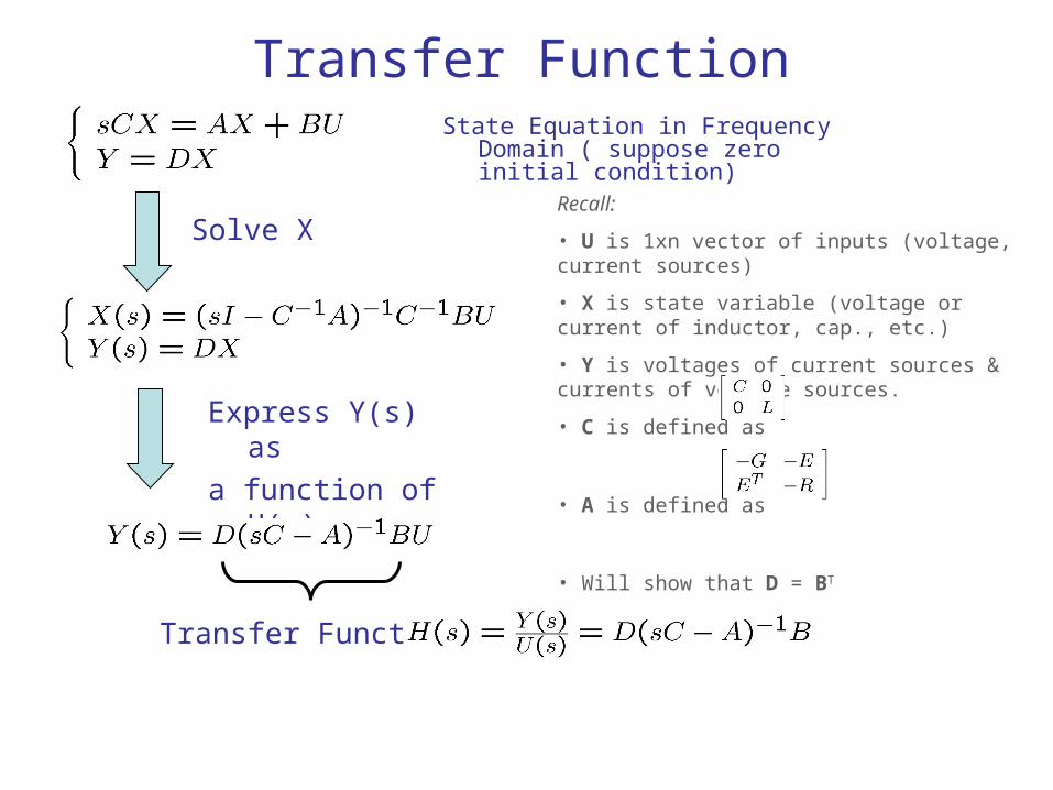
Transfer FunctionState Equation in Frequency Domain (

suppose zero initial condition)

Express Y(s) as

a function of U(s)

Solve X

Transfer Function:

Recall:

• U is 1xn vector of inputs (voltage, current sources)

• X is state variable (voltage or current of inductor, cap., etc.)

• Y is voltages of current sources & currents of voltage sources.

• C is defined as

• A is defined as

• Will show that D = BT

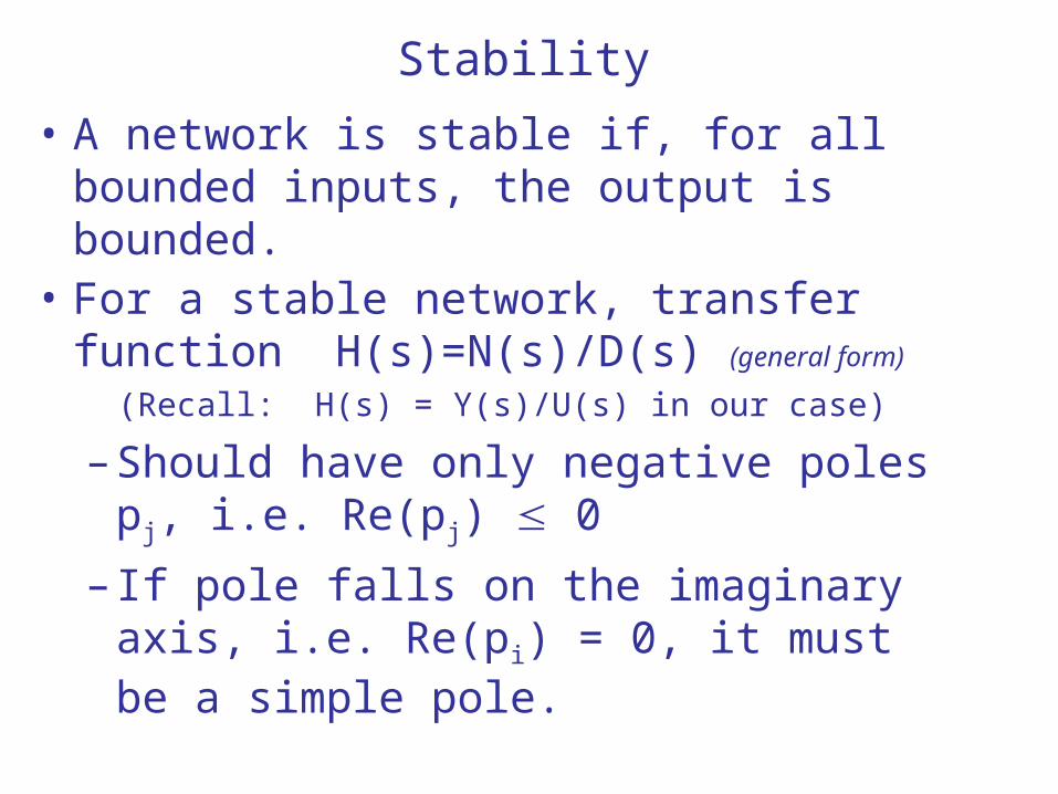
Stability

• A network is stable if, for all bounded inputs, the output is bounded.

• For a stable network, transfer function H(s)=N(s)/D(s) (general form)

(Recall: H(s) = Y(s)/U(s) in our case)

– Should have only negative poles pj, i.e. Re(pj) 0

– If pole falls on the imaginary axis, i.e. Re(pi) = 0, it must be a simple pole.

Passivity

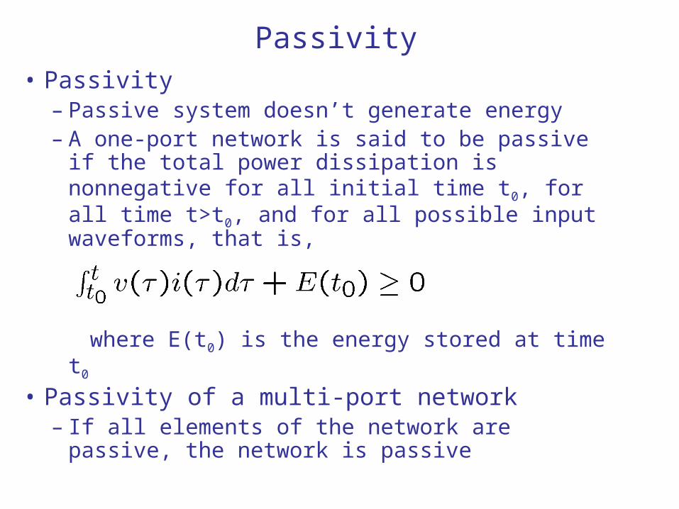
• Passivity – Passive system doesn’t generate energy– A one-port network is said to be passive if the

total power dissipation is nonnegative for all initial time t0, for all time t>t0, and for all possible input waveforms, that is,

where E(t0) is the energy stored at time t0

• Passivity of a multi-port network– If all elements of the network are passive, the

network is passive

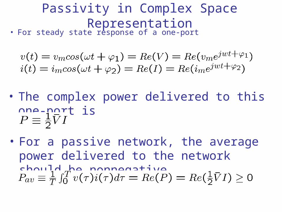
Passivity in Complex Space Representation• For steady state response of a one-port

• The complex power delivered to this one-port is

• For a passive network, the average power delivered to the network should be nonnegative

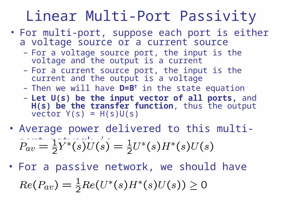
Linear Multi-Port Passivity• For multi-port, suppose each port is either a voltage

source or a current source– For a voltage source port, the input is the voltage and the

output is a current– For a current source port, the input is the current and the

output is a voltage– Then we will have D=BT in the state equation– Let U(s) be the input vector of all ports, and H(s) be the

transfer function, thus the output vector Y(s) = H(s)U(s)

• Average power delivered to this multi-port network is

• For a passive network, we should have

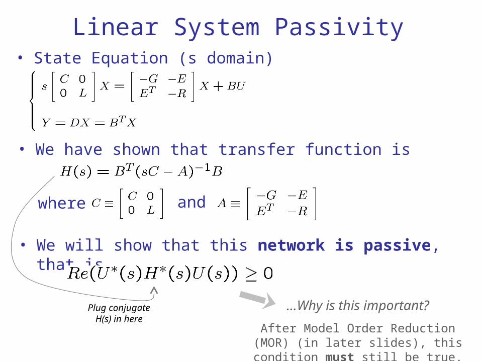
Linear System Passivity• State Equation (s domain)

• We have shown that transfer function is

where

• We will show that this network is passive, that is

and

Plug conjugate H(s) in here

…Why is this important?

After Model Order Reduction (MOR) (in later slides), this condition must still be true.

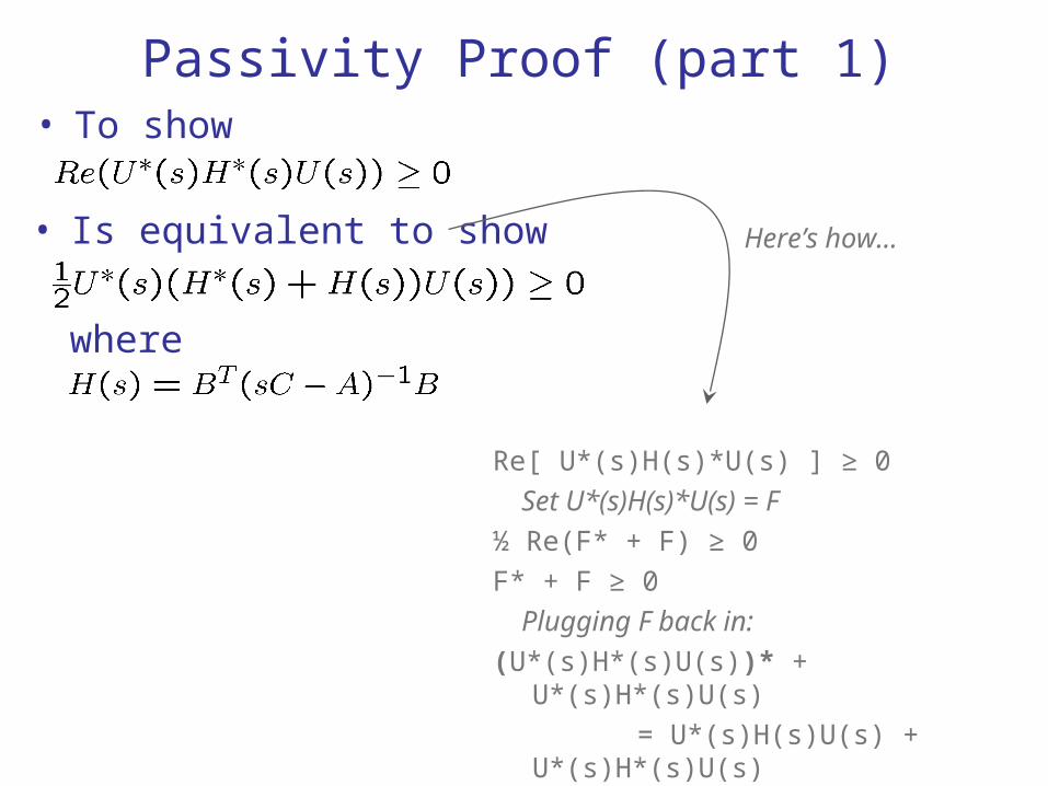
Passivity Proof (part 1)• To show

• Is equivalent to show

where

Re[ U*(s)H(s)*U(s) ] ≥ 0

Set U*(s)H(s)*U(s) = F

½ Re(F* + F) ≥ 0

F* + F ≥ 0

Plugging F back in:

(U*(s)H*(s)U(s))* + U*(s)H*(s)U(s)

= U*(s)H(s)U(s) + U*(s)H*(s)U(s)

= U*(s) (H(s) + H*(s)) U(s) ≥ 0

Here’s how…

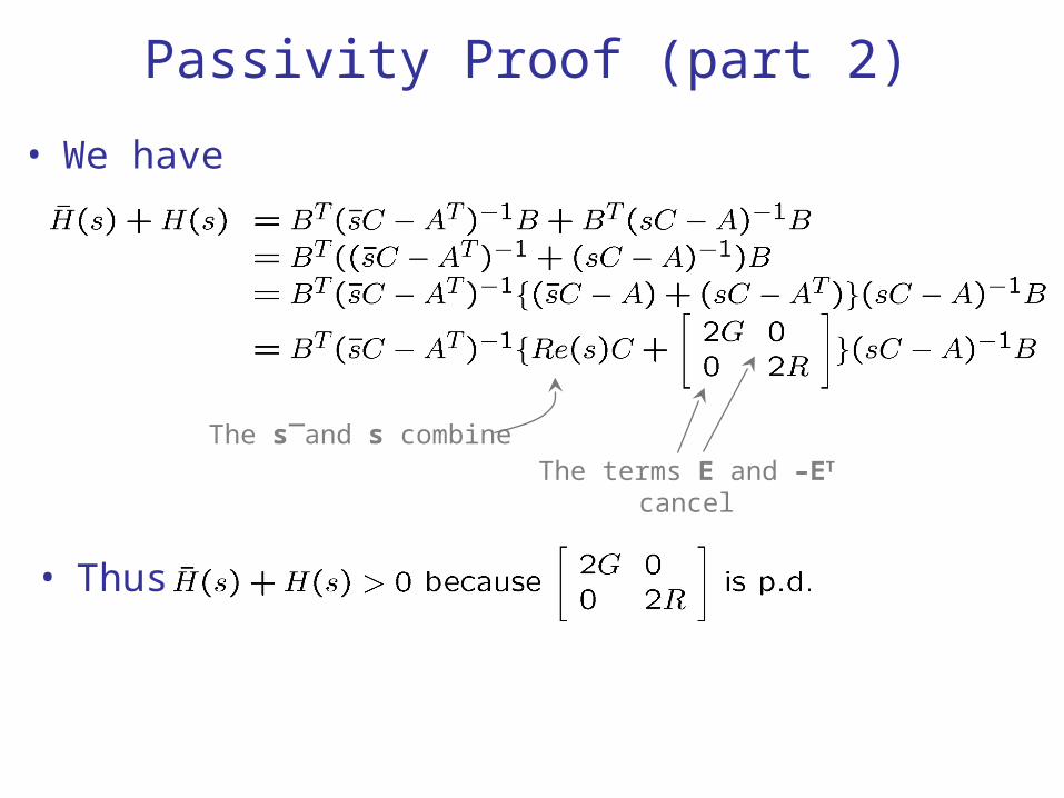
Passivity Proof (part 2)

• We have

• Thus

The s and s combine_

The terms E and –ET cancel

Passivity and Stability

• A passive network is stable.

• However, a stable network is not necessarily passive.

• All poles could be on LHS, but some could be negative!

• A interconnect network of stable components is not necessarily stable.

• The interconnection of passive components is passive.

Model Order Reduction (MOR)• MOR techniques are used to build a reduced

order model to approximate the original circuitR L

C G

i2(t)i1(t)

v1(t)

R L

C G

R L

C G

R L

C G

i1(t)

v1(t)

i2(t)

v2(t)

R L

C G

s uC x A x b

'' ' ' ' 's uC x A x b

Huge

Network Small

Network

MOR

Formulation

Realization

Model Order Reduction: Overview

• Explicit Moment Matching– AWE, Pade Approximation

• Implicit Moment Matching– Krylov Subspace Methods

• PRIMA, SPRIM

• Gaussian Elimination– TICER– Y-Delta Transformation

Moments Review• Transfer function

• Compare

• Moments

0

2 12 2 2 1 2 1 2

0 0 0 0

( ) ( )

1 ( 1)( ) ( ) ( ) ( ) ( )

2! (2 1)!

st

qq q q

H s e h t dt

h t dt th t dt s t h t dt s t h t dt s O sq

2 2 1 20 1 2 2 1( ) ( )q q

qH s m m s m s m s O s

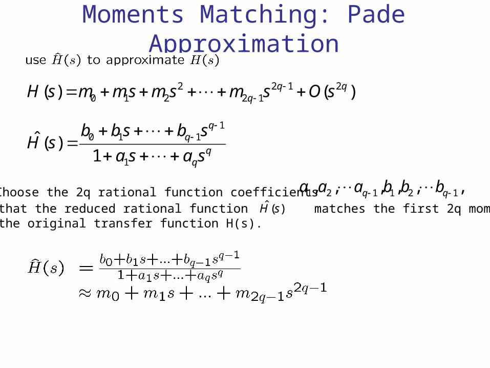
Moments Matching: Pade Approximation

qq

qq

sasa

sbsbbsH

1

1110

1)(ˆ

Choose the 2q rational function coefficientsSo that the reduced rational function matches the first 2q moments of the original transfer function H(s).

,,,,,, 121121 qq bbbaaa ˆ ( )H s

2 2 1 20 1 2 2 1( ) ( )q q

qH s m m s m s m s O s

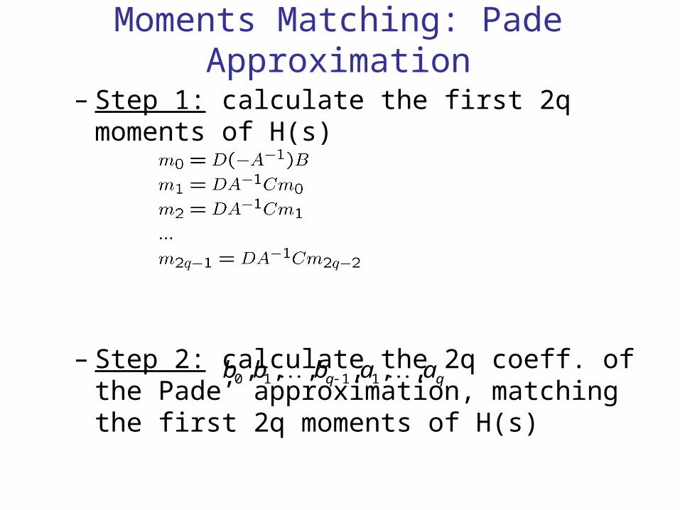
Moments Matching: Pade Approximation

– Step 1: calculate the first 2q moments of H(s)

– Step 2: calculate the 2q coeff. of the Pade’ approximation, matching the first 2q moments of H(s) qq aabbb ,,,,,, 1110

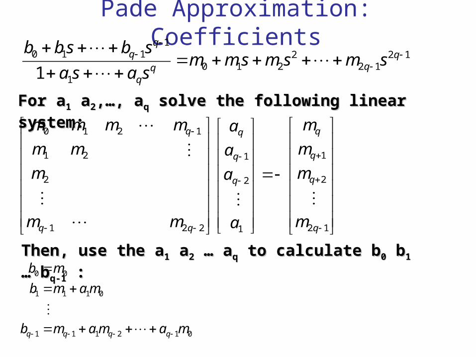
Pade Approximation: Coefficients12

122

2101

1110

1

q

qqq

qq smsmsmmsasa

sbsbb

012111

0111

00

mamamb

mamb

mb

qqqq

For aFor a11 a a22,…, a,…, aqq solve the following linear system: solve the following linear system:

12

2

1

1

2

1

221

2

21

1210

q

q

q

q

q

q

q

qq

q

m

m

m

m

a

a

a

a

mm

m

mm

mmmm

Then, use the aThen, use the a11 a a22 … a … aqq to calculate b to calculate b00 b b11 … b … bq-1q-1 : :

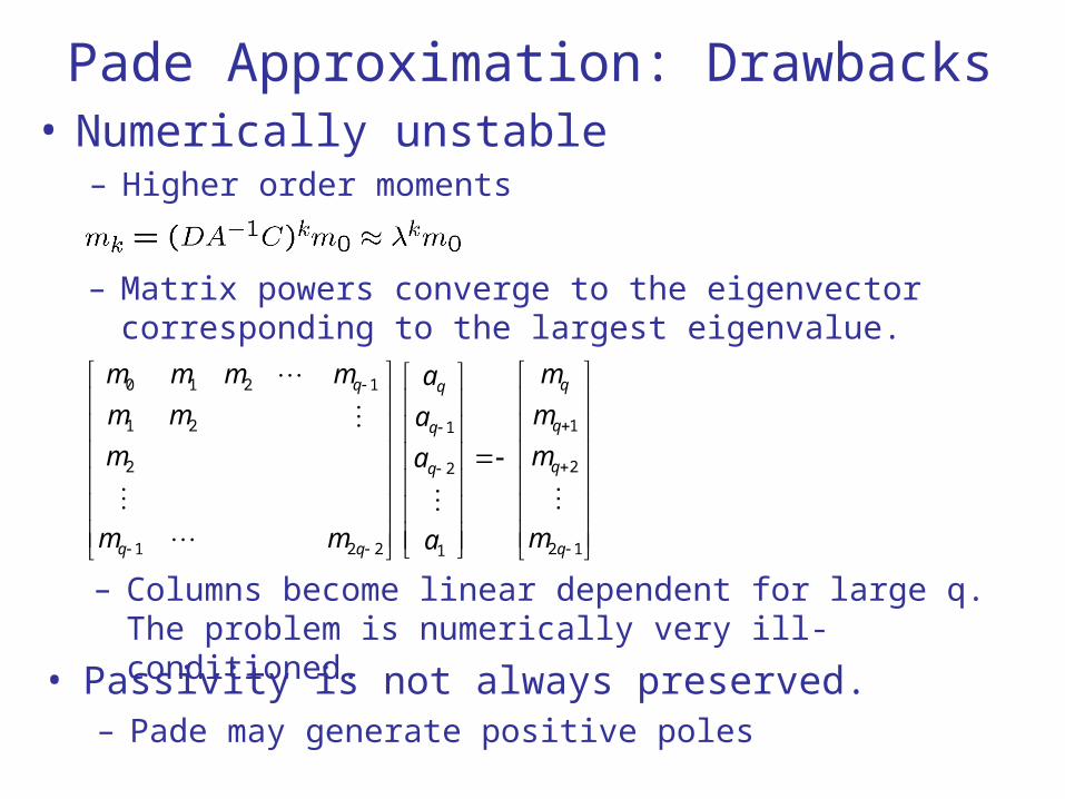
Pade Approximation: Drawbacks• Numerically unstable

– Higher order moments

– Matrix powers converge to the eigenvector corresponding to the largest eigenvalue.

12

2

1

1

2

1

221

2

21

1210

q

q

q

q

q

q

q

qq

q

m

m

m

m

a

a

a

a

mm

m

mm

mmmm

– Columns become linear dependent for large q. The problem is numerically very ill-conditioned.

• Passivity is not always preserved.– Pade may generate positive poles