CSE 326: Data Structures

Introduction

1Data Structures - Introduction

Class Overview

• Introduction to many of the basic data structures used in computer software– Understand the data structures– Analyze the algorithms that use them– Know when to apply them

• Practice design and analysis of data structures.• Practice using these data structures by writing

programs.• Make the transformation from programmer to

computer scientist

2Data Structures - Introduction

Goals

• You will understand– what the tools are for storing and processing common

data types– which tools are appropriate for which need

• So that you can– make good design choices as a developer, project

manager, or system customer• You will be able to

– Justify your design decisions via formal reasoning– Communicate ideas about programs clearly and

precisely

3Data Structures - Introduction

Goals

“I will, in fact, claim that the difference between a bad programmer and a good one is whether he considers his code or his data structures more important. Bad programmers worry about the code. Good programmers worry about data structures and their relationships.”

Linus Torvalds, 2006

4Data Structures - Introduction

Goals

“Show me your flowcharts and conceal your tables, and I shall continue to be mystified. Show me your tables, and I won’t usually need your flowcharts; they’ll be obvious.”

Fred Brooks, 1975

5Data Structures - Introduction

Data Structures

“Clever” ways to organize information in order to enable efficient computation

– What do we mean by clever?– What do we mean by efficient?

6Data Structures - Introduction

Picking the best Data Structure for the job

• The data structure you pick needs to support the operations you need

• Ideally it supports the operations you will use most often in an efficient manner

• Examples of operations:– A List with operations insert and delete– A Stack with operations push and pop

7Data Structures - Introduction

Terminology

• Abstract Data Type (ADT)– Mathematical description of an object with set of

operations on the object. Useful building block.• Algorithm

– A high level, language independent, description of a step-by-step process

• Data structure– A specific family of algorithms for implementing an

abstract data type.• Implementation of data structure

– A specific implementation in a specific language

8Data Structures - Introduction

Terminology examples

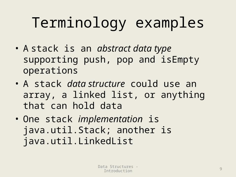
• A stack is an abstract data type supporting push, pop and isEmpty operations

• A stack data structure could use an array, a linked list, or anything that can hold data

• One stack implementation is java.util.Stack; another is java.util.LinkedList

9Data Structures - Introduction

Concepts vs. Mechanisms

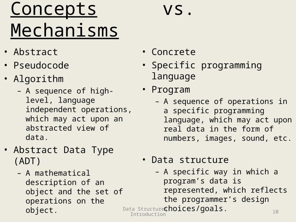
• Abstract• Pseudocode• Algorithm

– A sequence of high-level, language independent operations, which may act upon an abstracted view of data.

• Abstract Data Type (ADT)– A mathematical description

of an object and the set of operations on the object.

• Concrete• Specific programming language• Program

– A sequence of operations in a specific programming language, which may act upon real data in the form of numbers, images, sound, etc.

• Data structure– A specific way in which a

program’s data is represented, which reflects the programmer’s design choices/goals.

10Data Structures - Introduction

Why So Many Data Structures?

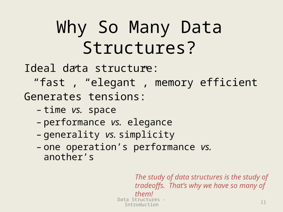
Ideal data structure:“fast”, “elegant”, memory efficient

Generates tensions:– time vs. space– performance vs. elegance– generality vs. simplicity– one operation’s performance vs. another’s

The study of data structures is the study of tradeoffs. That’s why we have so many of them!

11Data Structures - Introduction

Today’s Outline

• Introductions

• Administrative Info

• What is this course about?

• Review: Queues and stacks

12Data Structures - Introduction

First Example: Queue ADT

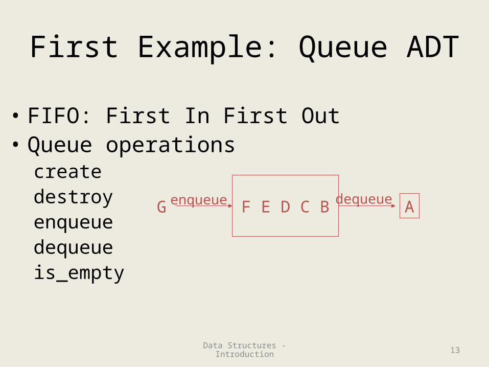
• FIFO: First In First Out• Queue operations

createdestroyenqueuedequeueis_empty

F E D C Benqueue dequeueG A

13Data Structures - Introduction

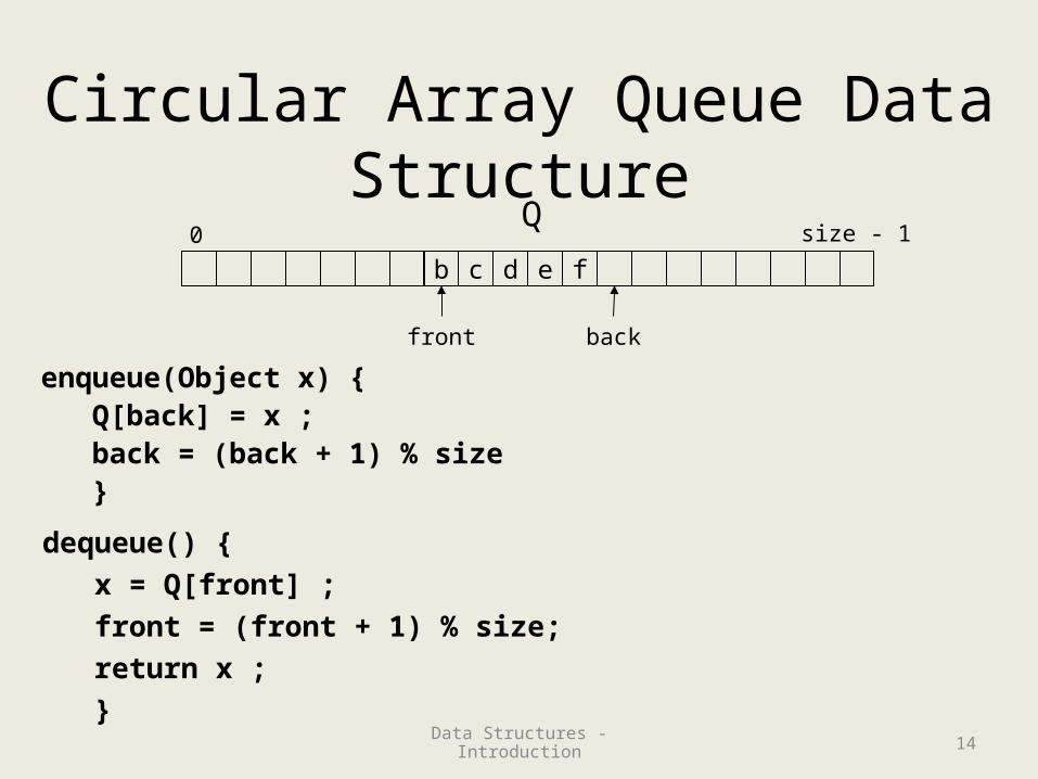
Circular Array Queue Data Structure

enqueue(Object x) {Q[back] = x ;back = (back + 1) % size}

b c d e f

Q0 size - 1

front back

dequeue() {

x = Q[front] ;

front = (front + 1) % size;

return x ;

}14Data Structures - Introduction

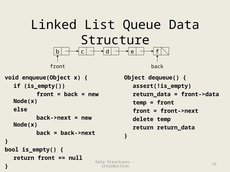
Linked List Queue Data Structureb c d e f

front back

void enqueue(Object x) {

if (is_empty())

front = back = new Node(x)

else

back->next = new Node(x)

back = back->next

}

bool is_empty() {

return front == null

}

Object dequeue() {

assert(!is_empty)

return_data = front->data

temp = front

front = front->next

delete temp

return return_data

}

15Data Structures - Introduction

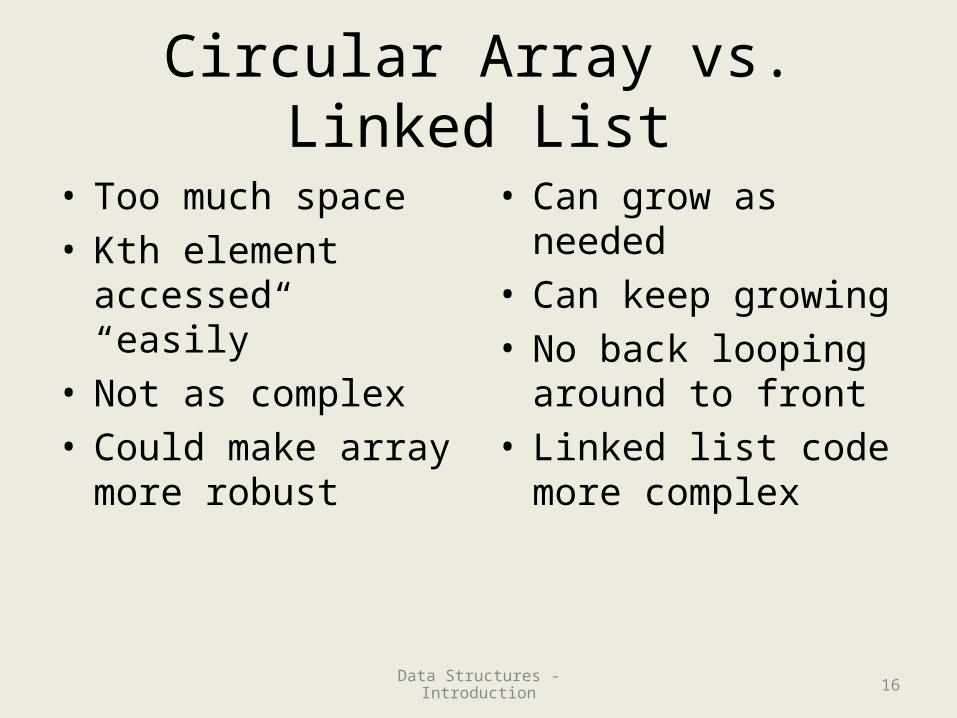
Circular Array vs. Linked List

• Too much space• Kth element accessed

“easily”• Not as complex• Could make array

more robust

• Can grow as needed• Can keep growing• No back looping

around to front• Linked list code more

complex

16Data Structures - Introduction

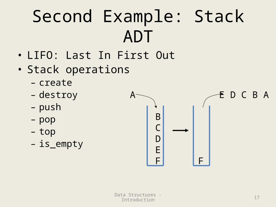
Second Example: Stack ADT

• LIFO: Last In First Out• Stack operations

– create– destroy– push– pop– top– is_empty

A

BCDEF

E D C B A

F

17Data Structures - Introduction

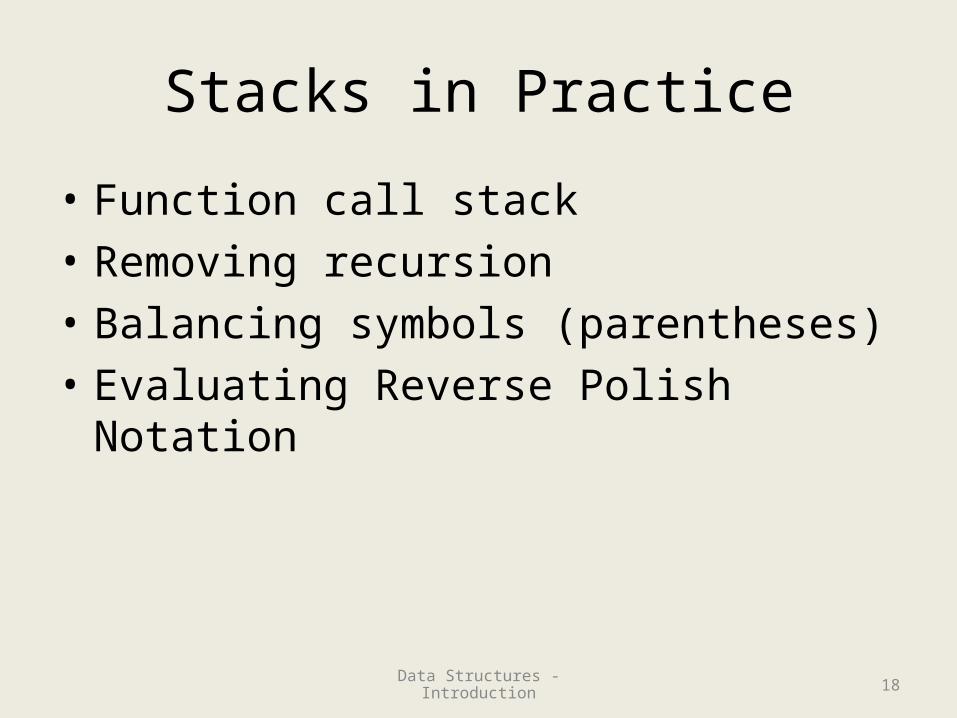
Stacks in Practice

• Function call stack

• Removing recursion

• Balancing symbols (parentheses)

• Evaluating Reverse Polish Notation

18Data Structures - Introduction

Data Structures

Asymptotic Analysis

19Data Structures - Introduction

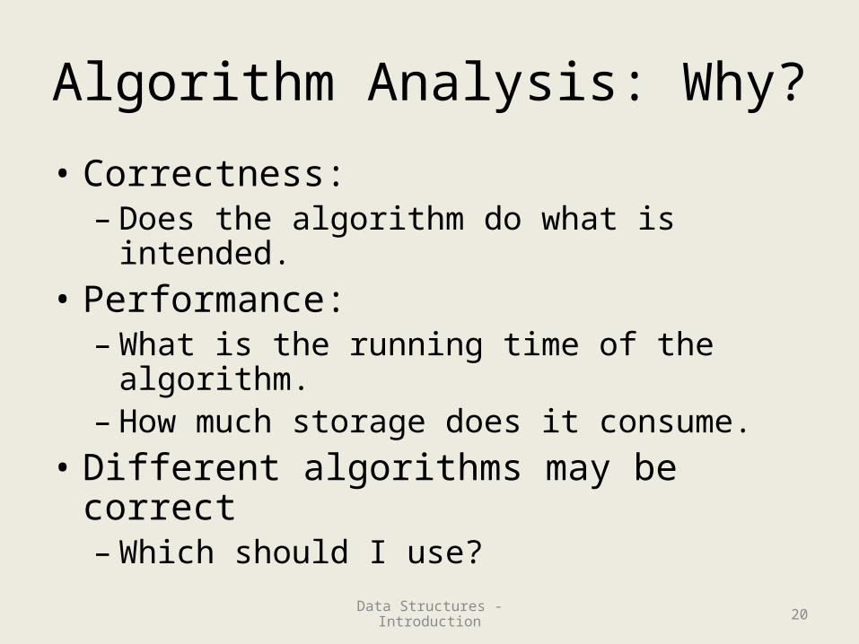
Algorithm Analysis: Why?

• Correctness:– Does the algorithm do what is intended.

• Performance:– What is the running time of the algorithm.– How much storage does it consume.

• Different algorithms may be correct– Which should I use?

20Data Structures - Introduction

Recursive algorithm for sum

• Write a recursive function to find the sum of the first n integers stored in array v.

21Data Structures - Introduction

Proof by Induction

• Basis Step: The algorithm is correct for a base case or two by inspection.

• Inductive Hypothesis (n=k): Assume that the algorithm works correctly for the first k cases.

• Inductive Step (n=k+1): Given the hypothesis above, show that the k+1 case will be calculated correctly.

22Data Structures - Introduction

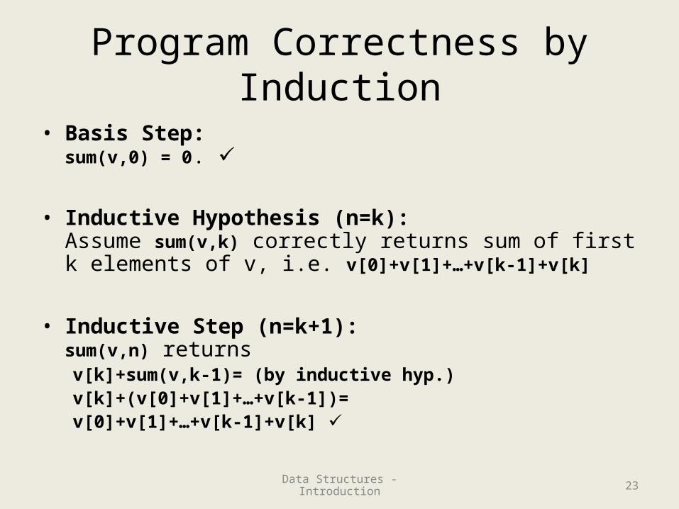
Program Correctness by Induction

• Basis Step:sum(v,0) = 0.

• Inductive Hypothesis (n=k): Assume sum(v,k) correctly returns sum of first k elements of v, i.e. v[0]+v[1]+…+v[k-1]+v[k]

• Inductive Step (n=k+1): sum(v,n) returnsv[k]+sum(v,k-1)= (by inductive hyp.)v[k]+(v[0]+v[1]+…+v[k-1])=v[0]+v[1]+…+v[k-1]+v[k]

23Data Structures - Introduction

Algorithms vs Programs

• Proving correctness of an algorithm is very important– a well designed algorithm is guaranteed to work correctly and its

performance can be estimated

• Proving correctness of a program (an implementation) is fraught with weird bugs– Abstract Data Types are a way to bridge the gap between

mathematical algorithms and programs

24Data Structures - Introduction

Comparing Two Algorithms

GOAL: Sort a list of names

“I’ll buy a faster CPU”

“I’ll use C++ instead of Java – wicked fast!”

“Ooh look, the –O4 flag!”

“Who cares how I do it, I’ll add more memory!”

“Can’t I just get the data pre-sorted??”

25Data Structures - Introduction

Comparing Two Algorithms

• What we want:– Rough Estimate– Ignores Details

• Really, independent of details – Coding tricks, CPU speed, compiler

optimizations, …– These would help any algorithms equally– Don’t just care about running time – not a good

enough measure

26Data Structures - Introduction

Big-O Analysis

• Ignores “details”

• What details?– CPU speed– Programming language used– Amount of memory– Compiler– Order of input– Size of input … sorta.

27Data Structures - Introduction

Analysis of Algorithms

• Efficiency measure– how long the program runs time complexity– how much memory it uses space complexity

• Why analyze at all?– Decide what algorithm to implement before

actually doing it– Given code, get a sense for where bottlenecks

must be, without actually measuring it

28Data Structures - Introduction

Asymptotic Analysis

• Complexity as a function of input size nT(n) = 4n + 5

T(n) = 0.5 n log n - 2n + 7

T(n) = 2n + n3 + 3n

• What happens as n grows?

29Data Structures - Introduction

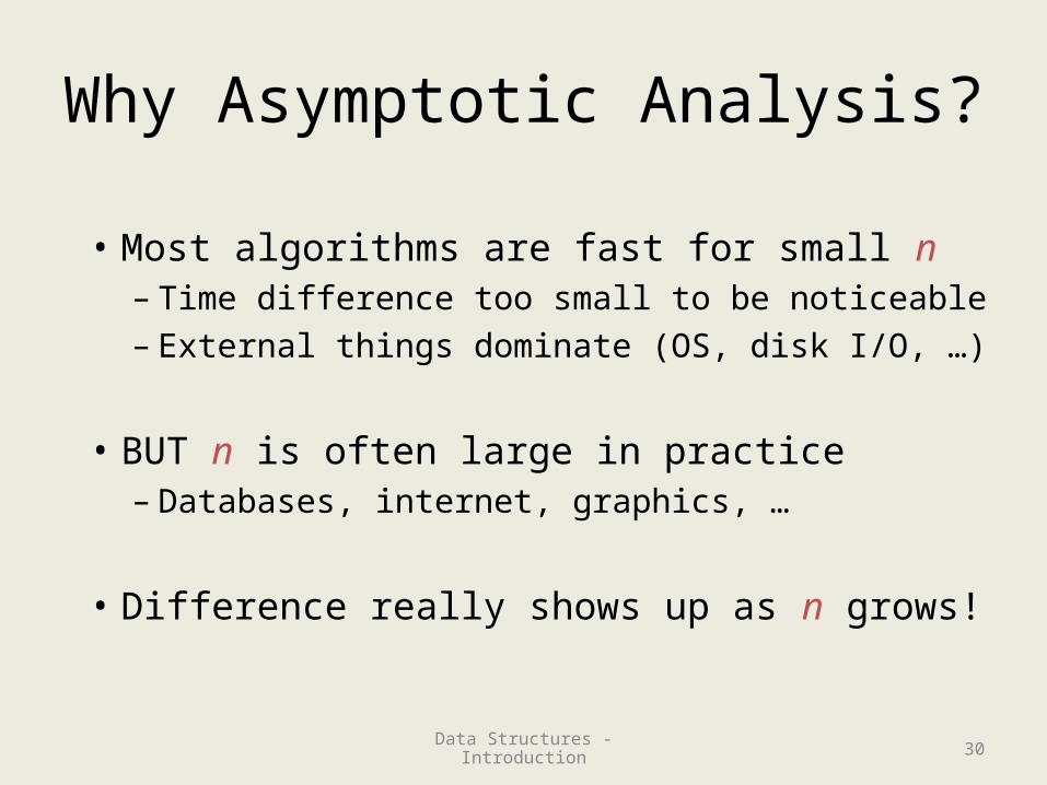
Why Asymptotic Analysis?

• Most algorithms are fast for small n – Time difference too small to be noticeable– External things dominate (OS, disk I/O, …)

• BUT n is often large in practice– Databases, internet, graphics, …

• Difference really shows up as n grows!30Data Structures - Introduction

Exercise - Searching

bool ArrayFind( int array[], int n, int key){// Insert your algorithm here

}

2 3 5 16 37 50 73 75 126

What algorithm would you choose to implement this code

snippet?31Data Structures - Introduction

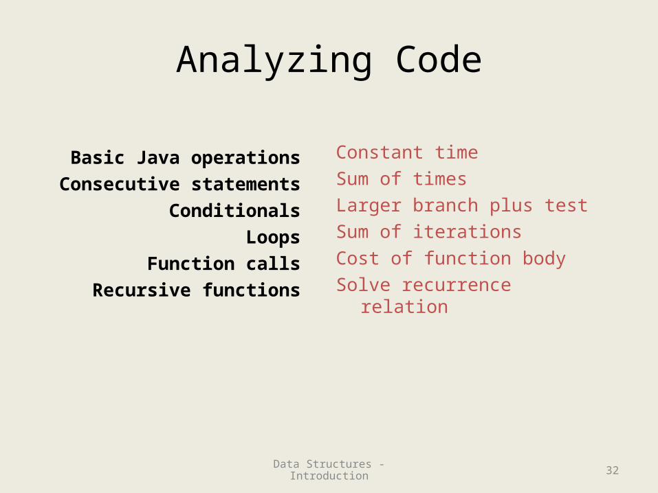
Analyzing Code

Basic Java operations

Consecutive statements

Conditionals

Loops

Function calls

Recursive functions

Constant time

Sum of times

Larger branch plus test

Sum of iterations

Cost of function body

Solve recurrence relation

32Data Structures - Introduction

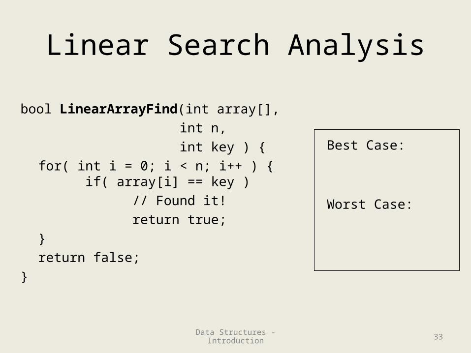
Linear Search Analysis

bool LinearArrayFind(int array[],

int n,

int key ) {

for( int i = 0; i < n; i++ ) {if( array[i] == key )

// Found it!

return true;

}

return false;

}

Best Case:

Worst Case:

33Data Structures - Introduction

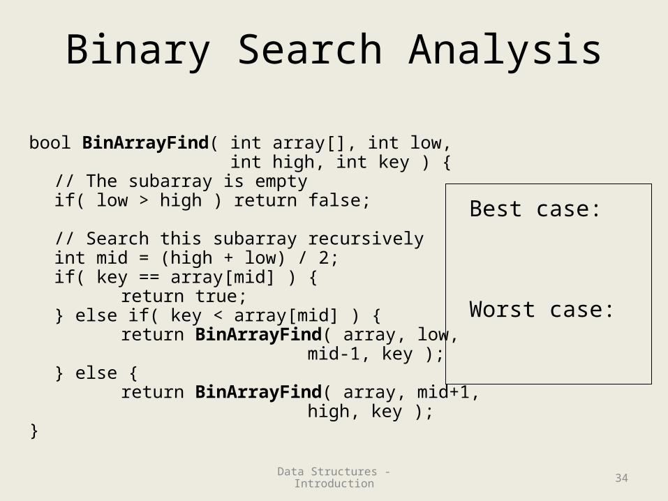
Binary Search Analysis

bool BinArrayFind( int array[], int low, int high, int key ) {

// The subarray is emptyif( low > high ) return false;

// Search this subarray recursivelyint mid = (high + low) / 2;if( key == array[mid] ) {

return true;} else if( key < array[mid] ) {

return BinArrayFind( array, low, mid-1, key );

} else {return BinArrayFind( array, mid+1,

high, key );}

Best case:

Worst case:

34Data Structures - Introduction

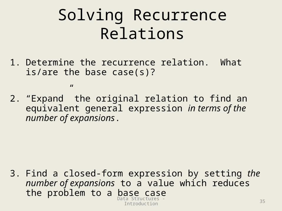
Solving Recurrence Relations

1. Determine the recurrence relation. What is/are the base case(s)?

2. “Expand” the original relation to find an equivalent general expression in terms of the number of expansions.

3. Find a closed-form expression by setting the number of expansions to a value which reduces the problem to a base case

35Data Structures - Introduction

Data Structures

Asymptotic Analysis

36Data Structures - Introduction

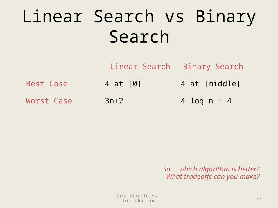
Linear Search vs Binary Search

Linear Search Binary Search

Best Case 4 at [0] 4 at [middle]

Worst Case 3n+2 4 log n + 4

So … which algorithm is better?What tradeoffs can you make?

37Data Structures - Introduction

Fast Computer vs. Slow Computer

38

Fast Computer vs. Smart Programmer (round 1)

39

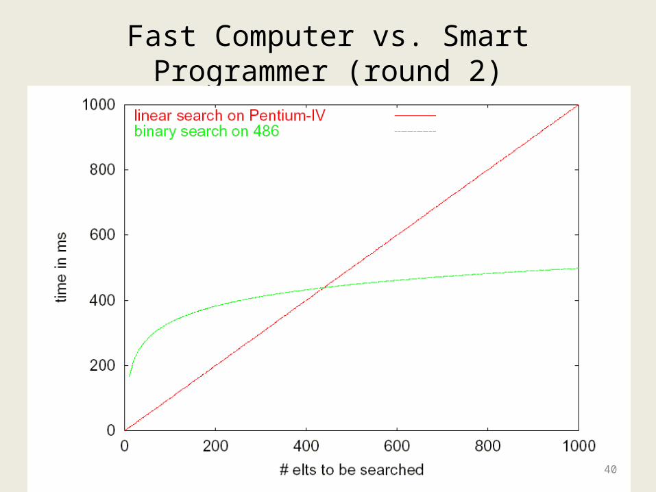
Fast Computer vs. Smart Programmer (round 2)

40

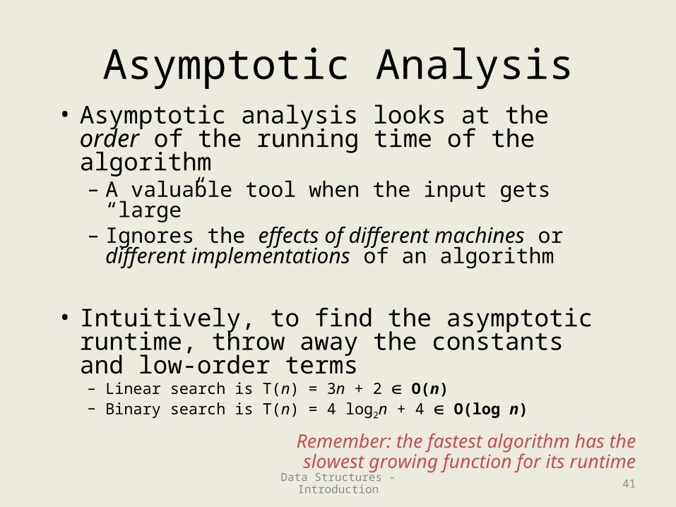
Asymptotic Analysis• Asymptotic analysis looks at the order of

the running time of the algorithm– A valuable tool when the input gets “large”– Ignores the effects of different machines or

different implementations of an algorithm

• Intuitively, to find the asymptotic runtime, throw away the constants and low-order terms– Linear search is T(n) = 3n + 2 O(n)– Binary search is T(n) = 4 log2n + 4 O(log n)

Remember: the fastest algorithm has the slowest growing function for its runtime

41Data Structures - Introduction

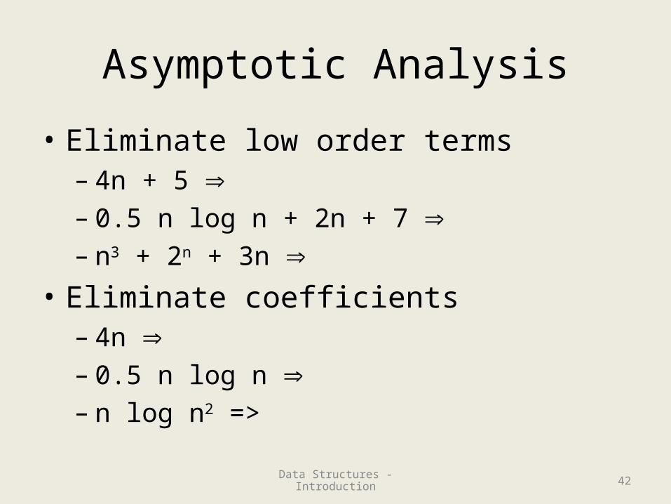
Asymptotic Analysis

• Eliminate low order terms– 4n + 5 – 0.5 n log n + 2n + 7 – n3 + 2n + 3n

• Eliminate coefficients– 4n – 0.5 n log n – n log n2 =>

42Data Structures - Introduction

Properties of Logs

• log AB = log A + log B• Proof:

• Similarly:– log(A/B) = log A – log B– log(AB) = B log A

• Any log is equivalent to log-base-2

BAAB

AB

BABABA

BA

logloglog

222

2,2)log(logloglog

loglog

2222

22

43Data Structures - Introduction

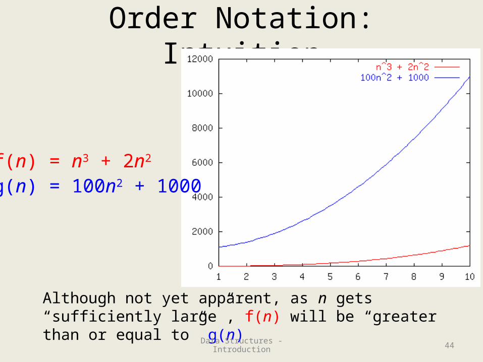
Order Notation: Intuition

Although not yet apparent, as n gets “sufficiently large”, f(n) will be “greater than or equal to” g(n)

f(n) = n3 + 2n2

g(n) = 100n2 + 1000

44Data Structures - Introduction

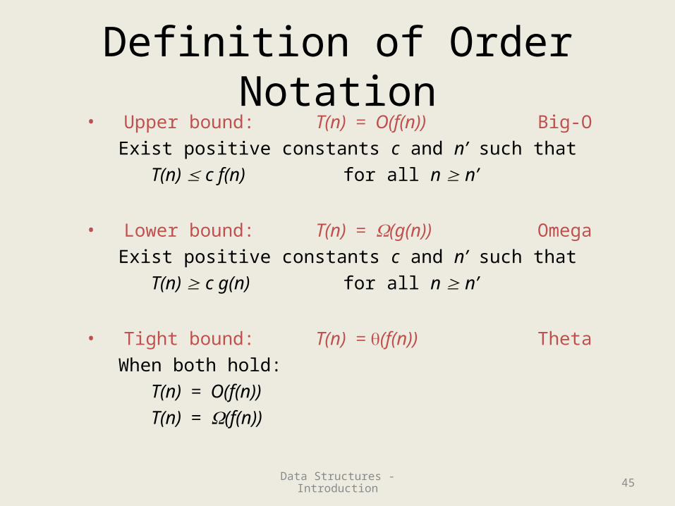
Definition of Order Notation• Upper bound: T(n) = O(f(n)) Big-O

Exist positive constants c and n’ such that

T(n) c f(n) for all n n’

• Lower bound: T(n) = (g(n))Omega

Exist positive constants c and n’ such that

T(n) c g(n) for all n n’

• Tight bound: T(n) = (f(n)) Theta

When both hold:

T(n) = O(f(n))

T(n) = (f(n))

45Data Structures - Introduction

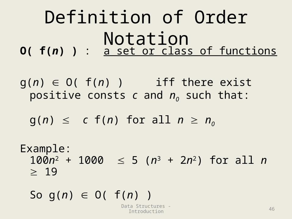
Definition of Order NotationO( f(n) ) : a set or class of functions

g(n) O( f(n) ) iff there exist positive consts c and n0 such that:

g(n) c f(n) for all n n0

Example:100n2 + 1000 5 (n3 + 2n2) for all n 19

So g(n) O( f(n) )46Data Structures - Introduction

Order Notation: Example

100n2 + 1000 5 (n3 + 2n2) for all n 19

So f(n) O( g(n) )47Data Structures - Introduction

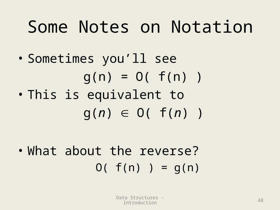
Some Notes on Notation

• Sometimes you’ll see

g(n) = O( f(n) )

• This is equivalent to

g(n) O( f(n) )

• What about the reverse?O( f(n) ) = g(n)

48Data Structures - Introduction

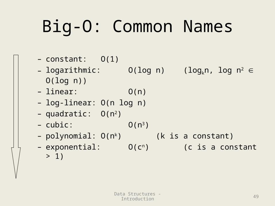
Big-O: Common Names

– constant: O(1)

– logarithmic: O(log n) (logkn, log n2 O(log n))

– linear: O(n)– log-linear: O(n log n)– quadratic: O(n2)– cubic: O(n3)– polynomial: O(nk) (k is a constant)– exponential: O(cn) (c is a constant > 1)

49Data Structures - Introduction

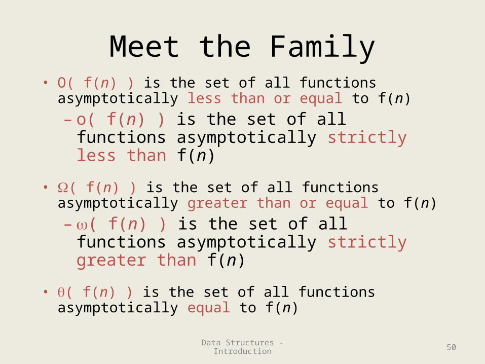
Meet the Family• O( f(n) ) is the set of all functions asymptotically less

than or equal to f(n)

– o( f(n) ) is the set of all functions asymptotically strictly less than f(n)

• ( f(n) ) is the set of all functions asymptotically greater than or equal to f(n)

– ( f(n) ) is the set of all functions asymptotically strictly greater than f(n)

• ( f(n) ) is the set of all functions asymptotically equal to f(n)

50Data Structures - Introduction

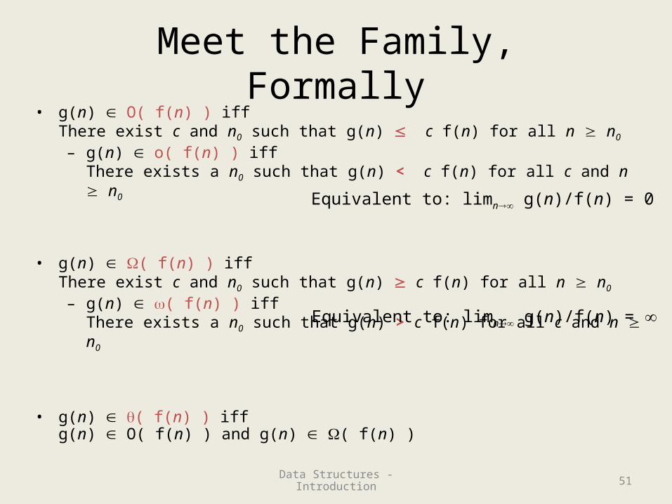
Meet the Family, Formally• g(n) O( f(n) ) iff

There exist c and n0 such that g(n) c f(n) for all n n0

– g(n) o( f(n) ) iff There exists a n0 such that g(n) < c f(n) for all c and n n0

• g(n) ( f(n) ) iffThere exist c and n0 such that g(n) c f(n) for all n n0

– g(n) ( f(n) ) iffThere exists a n0 such that g(n) > c f(n) for all c and n n0

• g(n) ( f(n) ) iffg(n) O( f(n) ) and g(n) ( f(n) )

Equivalent to: limn g(n)/f(n) = 0

Equivalent to: limn g(n)/f(n) =

51Data Structures - Introduction

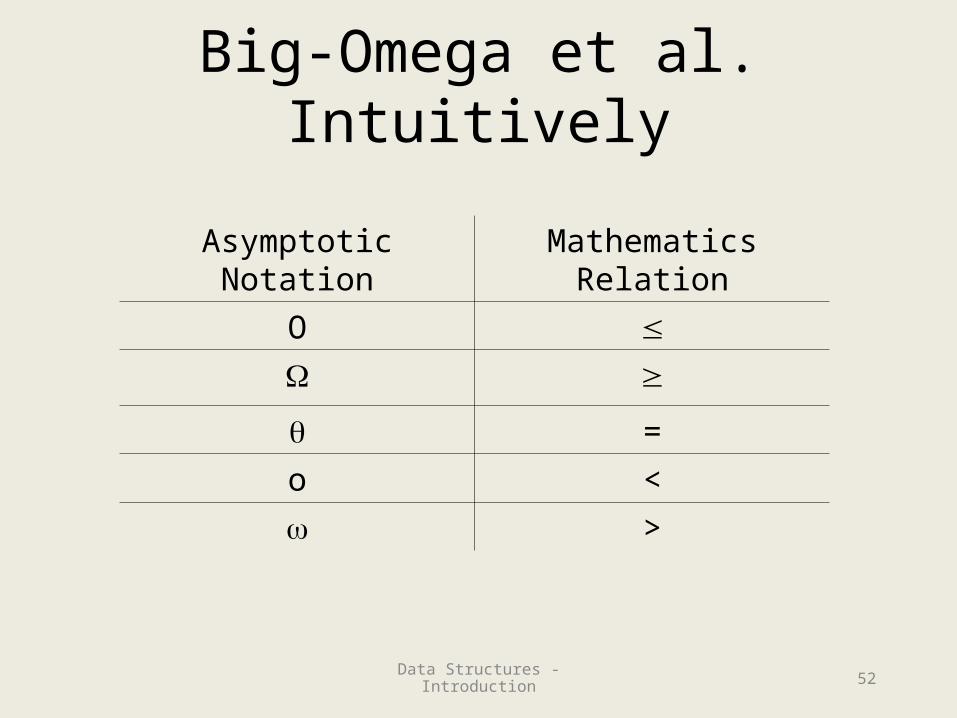
Big-Omega et al. Intuitively

Asymptotic Notation Mathematics Relation

O

=

o <

>

52Data Structures - Introduction

Pros and Cons of Asymptotic Analysis

53Data Structures - Introduction

Perspective: Kinds of Analysis• Running time may depend on actual data

input, not just length of input• Distinguish

– Worst Case• Your worst enemy is choosing input

– Best Case– Average Case

• Assumes some probabilistic distribution of inputs– Amortized

• Average time over many operations

54Data Structures - Introduction

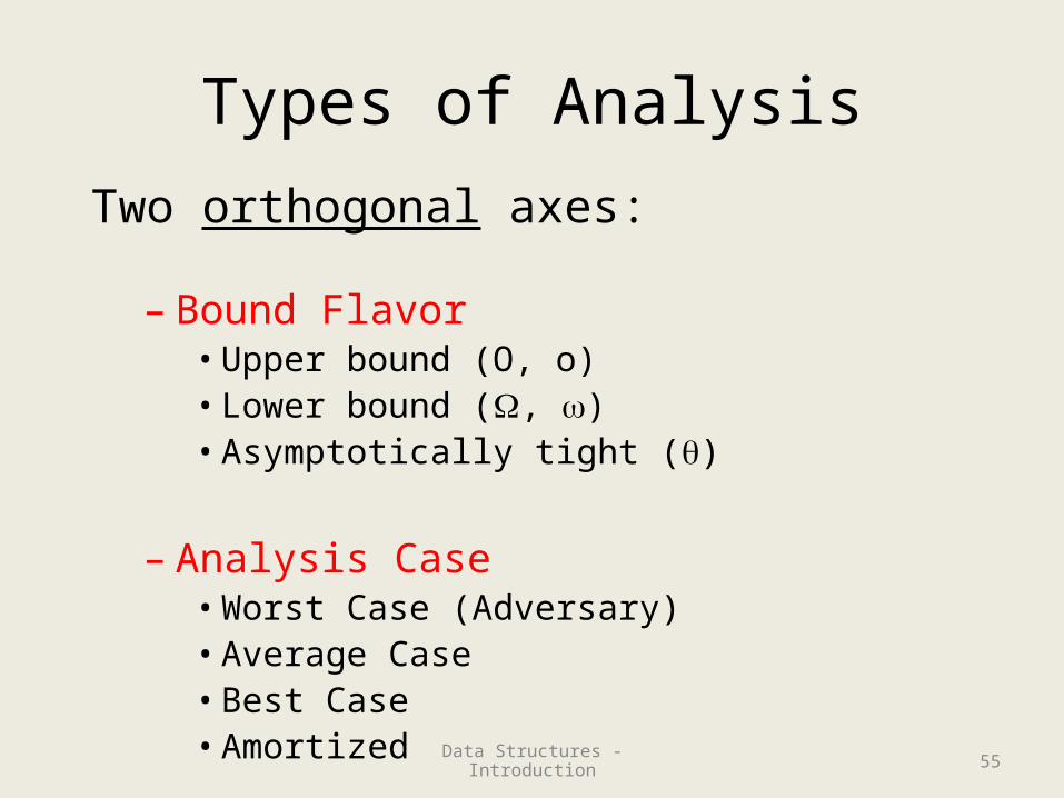
Types of Analysis

Two orthogonal axes:

– Bound Flavor• Upper bound (O, o)• Lower bound (, )• Asymptotically tight ()

– Analysis Case• Worst Case (Adversary)• Average Case• Best Case• Amortized 55Data Structures - Introduction

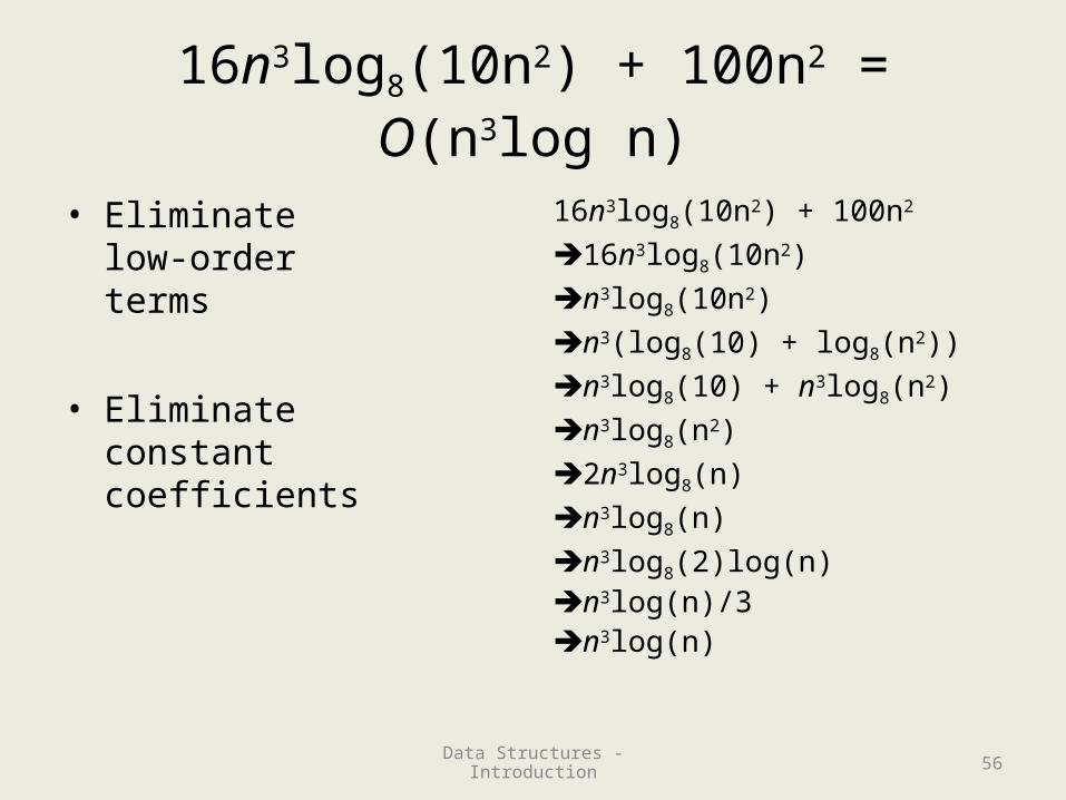
16n3log8(10n2) + 100n2 = O(n3log n)

• Eliminate low-order terms

• Eliminate constant coefficients

16n3log8(10n2) + 100n2

16n3log8(10n2)

n3log8(10n2)

n3(log8(10) + log8(n2))

n3log8(10) + n3log8(n2)

n3log8(n2)

2n3log8(n)

n3log8(n)

n3log8(2)log(n)n3log(n)/3n3log(n)

56Data Structures - Introduction