CSCI-1680Transport Layer III

Congestion Control Strikes Back

Based partly on lecture notes by David Mazières, Phil Levis, John Jannotti, Ion Stoica

Rodrigo Fonseca

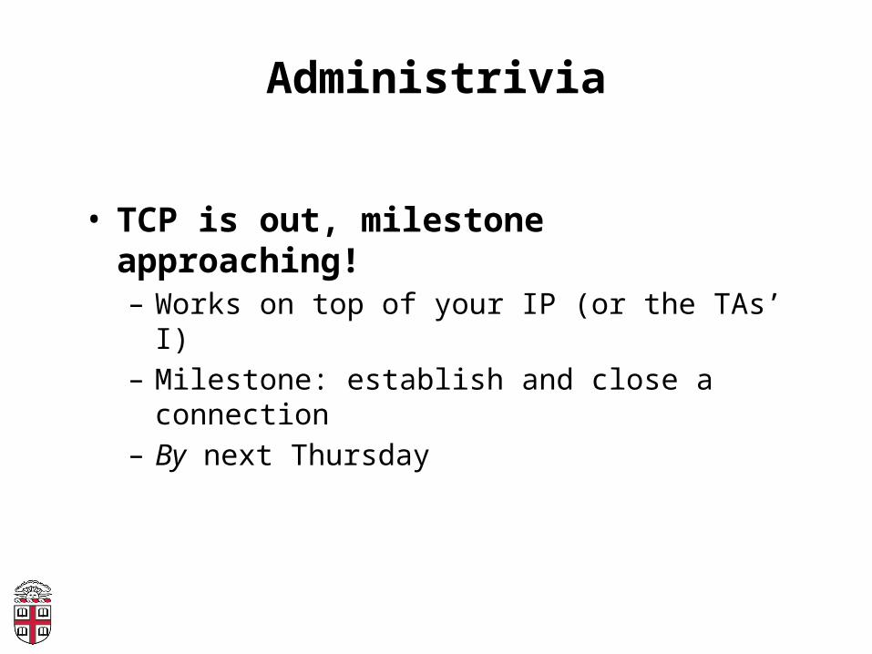
Administrivia

• TCP is out, milestone approaching!– Works on top of your IP (or the TAs’ I)– Milestone: establish and close a

connection– By next Thursday

Last Time

• Flow Control• Congestion Control

Today

• Congestion Control Continued– Quick Review– RTT Estimation

Quick Review

• Flow Control:– Receiver sets Advertised Window

• Congestion Control– Two states: Slow Start (SS) and Congestion

Avoidance (CA)– A window size threshold governs the state

transition• Window <= ssthresh: SS• Window > ssthresh: Congestion Avoidance

– States differ in how they respond to ACKs• Slow start: w = w + MSS (1 MSS per ACK)• Congestion Avoidance: w = w + MSS2/w (1 MSS per RTT)

– On loss event: set ssthresh = w/2, w = 1, slow start

AIMD

Flow Rate A

Flow

Rat

e B

Fair: A = B

Efficient: A+B = C

AIMD

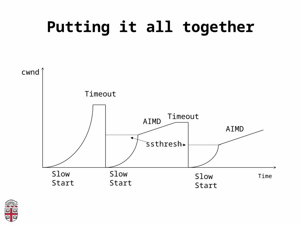
Putting it all together

Time

cwnd

Timeout

SlowStart

AIMD

ssthresh

Timeout

SlowStart

SlowStart

AIMD

Fast Recovery and Fast Retransmit

Time

cwnd

Slow Start

AI/MD

Fast retransmit

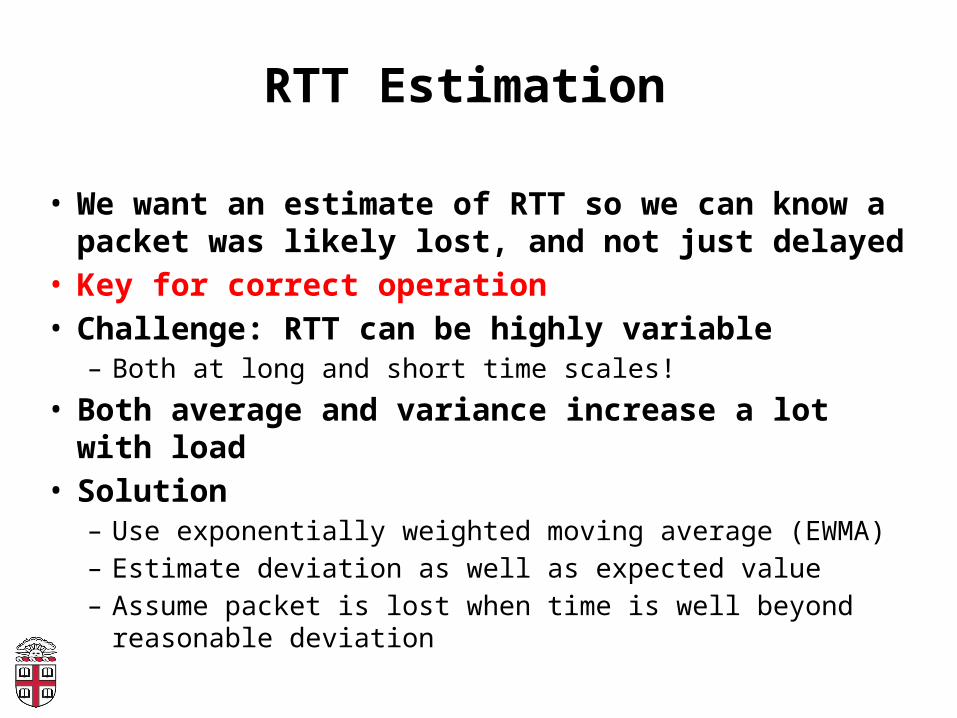
RTT Estimation

• We want an estimate of RTT so we can know a packet was likely lost, and not just delayed

• Key for correct operation• Challenge: RTT can be highly variable

– Both at long and short time scales!

• Both average and variance increase a lot with load

• Solution– Use exponentially weighted moving average (EWMA)– Estimate deviation as well as expected value– Assume packet is lost when time is well beyond

reasonable deviation

Originally• EstRTT = (1 – α) × EstRTT + α ×

SampleRTT• Timeout = 2 × EstRTT• Problem 1:

– in case of retransmission, ACK corresponds to which send?

– Solution: only sample for segments with no retransmission

• Problem 2:– does not take variance into account: too

aggressive when there is more load!

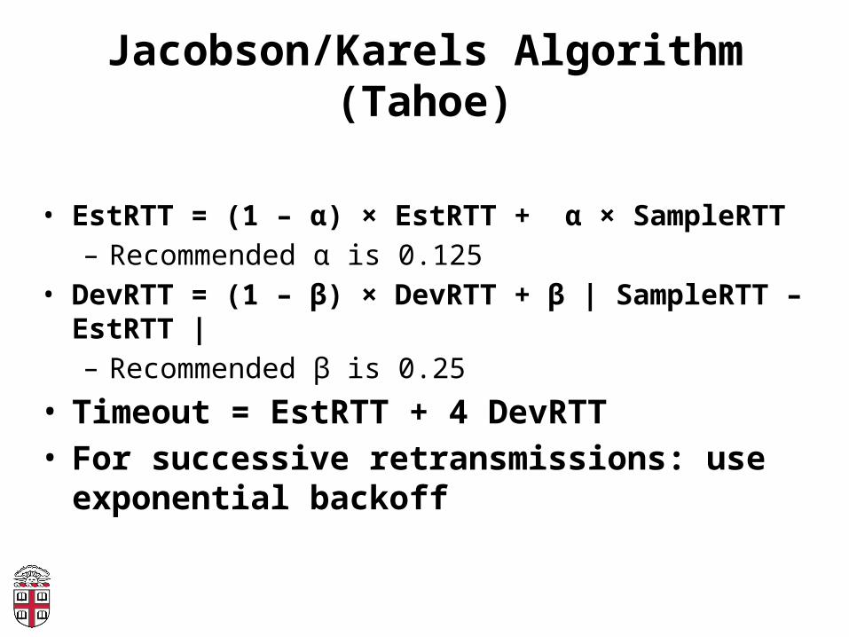
Jacobson/Karels Algorithm (Tahoe)

• EstRTT = (1 – α) × EstRTT + α × SampleRTT– Recommended α is 0.125

• DevRTT = (1 – β) × DevRTT + β | SampleRTT – EstRTT |– Recommended β is 0.25

• Timeout = EstRTT + 4 DevRTT• For successive retransmissions: use

exponential backoff

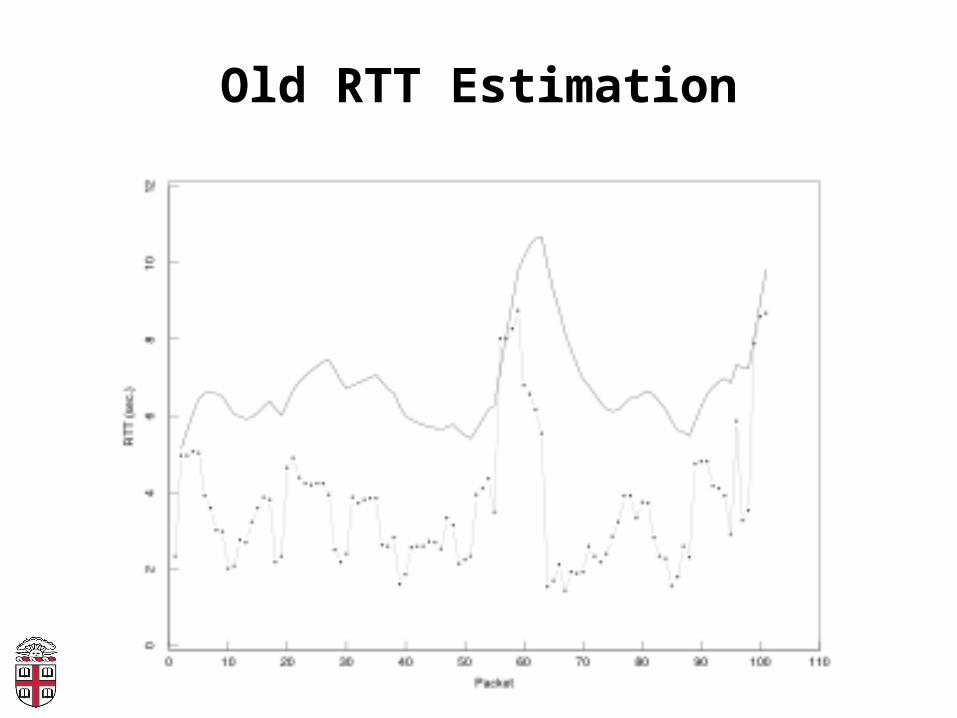
Old RTT Estimation

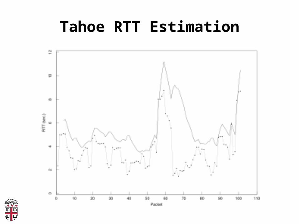
Tahoe RTT Estimation

Fun with TCP

• TCP Friendliness– Equation Based Rate Control

• Congestion Control versus Avoidance– Getting help from the network

• TCP on Lossy Links• Cheating TCP• Fair Queueing

TCP Friendliness• Can other protocols co-exist with

TCP?– E.g., if you want to write a video streaming

app using UDP, how to do congestion control?

RED

0

1

2

3

4

5

6

7

8

9

10

1 4 7 10 13 16 19 22 25 28 31Flow Number

Thro

ughp

ut(M

bps) 1 UDP Flow at 10MBps

31 TCP FlowsSharing a 10MBps link

TCP Friendliness• Can other protocols co-exist with TCP?– E.g., if you want to write a video streaming

app using UDP, how to do congestion control?

• Equation-based Congestion Control– Instead of implementing TCP’s CC,

estimate the rate at which TCP would send. Function of what?

– RTT, MSS, Loss

• Measure RTT, Loss, send at that rate!

TCP Throughput

• Assume a TCP connection of window W, round-trip time of RTT, segment size MSS– Sending Rate S = W x MSS / RTT (1)

• Drop: W = W/2– grows by MSS W/2 RTTs, until another drop at W ≈ W

• Average window then 0.75xS– From (1), S = 0.75 W MSS / RTT (2)

• Loss rate is 1 in number of packets between losses:– Loss = 1 / ( 1 + (W/2 + W/2+1 + W/2 + 2 + … + W)

= 1 / (3/8 W2) (3)

TCP Throughput (cont)

– Loss = 8/(3W2) (4)

– Substituting (4) in (2), S = 0.75 W MSS / RTT ,

Throughput ≈

€

⇒ W =8

3⋅ Loss

€

€

1.22 ×MSS

RTT⋅ Loss

• Equation-based rate control can be TCP friendly and have better properties, e.g., small jitter, fast ramp-up…

What Happens When Link is Lossy?

• Throughput ≈ 1 / sqrt(Loss)

0

10

20

30

40

50

60

1 26 51 76 101 126 151 176 201 226 251 276 301 326 351 376 401 426 451 476

p = 0

p = 1%

p = 10%

What can we do about it?

• Two types of losses: congestion and corruption

• One option: mask corruption losses from TCP– Retransmissions at the link layer– E.g. Snoop TCP: intercept duplicate

acknowledgments, retransmit locally, filter them from the sender

• Another option:– Tell the sender about the cause for the drop– Requires modification to the TCP endpoints

Congestion Avoidance

• TCP creates congestion to then back off– Queues at bottleneck link are often full:

increased delay– Sawtooth pattern: jitter

• Alternative strategy– Predict when congestion is about to happen– Reduce rate early

• Two approaches– Host centric: TCP Vegas– Router-centric: RED, DECBit

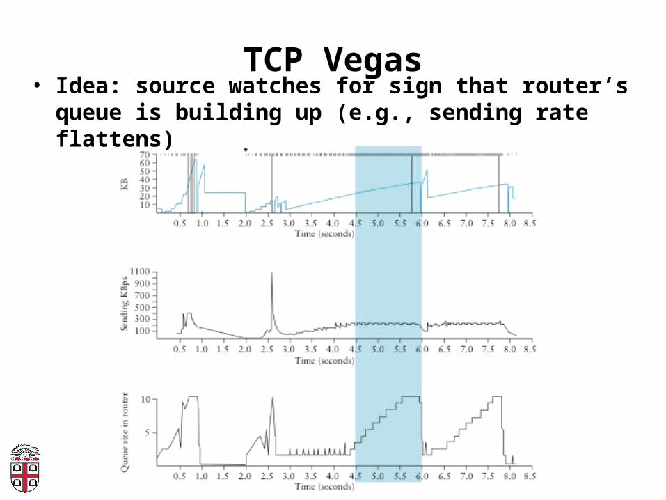
TCP Vegas• Idea: source watches for sign that router’s

queue is building up (e.g., sending rate flattens)

TCP Vegas• Compare Actual Rate (A) with Expected Rate (E)

– If E-A > β, decrease cwnd linearly : A isn’t responding– If E-A < α, increase cwnd linearly : Room for A to grow

Vegas

• Shorter router queues• Lower jitter• Problem:

– Doesn’t compete well with Reno. Why?– Reacts earlier, Reno is more aggressive,

ends up with higher bandwidth…

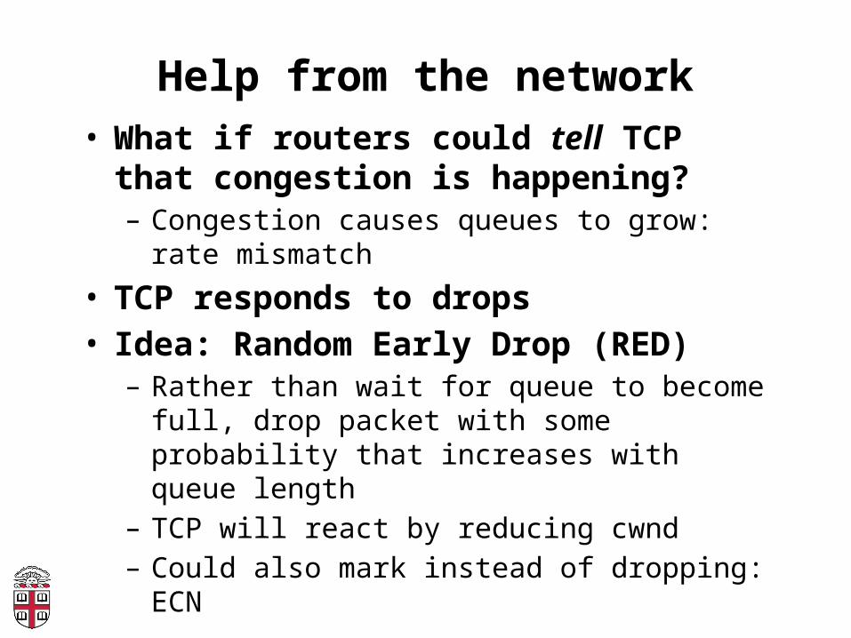
Help from the network

• What if routers could tell TCP that congestion is happening?– Congestion causes queues to grow: rate

mismatch

• TCP responds to drops• Idea: Random Early Drop (RED)

– Rather than wait for queue to become full, drop packet with some probability that increases with queue length

– TCP will react by reducing cwnd– Could also mark instead of dropping: ECN

RED Details• Compute average queue length

(EWMA)– Don’t want to react to very quick

fluctuations

RED Drop Probability

• Define two thresholds: MinThresh, MaxThresh• Drop probability:

• Improvements to spread drops (see book)

RED Advantages• Probability of dropping a packet of a particular flow is roughly proportional to the share of the bandwidth that flow is currently getting

• Higher network utilization with low delays

• Average queue length small, but can absorb bursts

• ECN– Similar to RED, but router sets bit in the

packet– Must be supported by both ends– Avoids retransmissions optionally dropped

packets

What happens if not everyone cooperates?

• TCP works extremely well when its assumptions are valid– All flows correctly implement congestion

control– Losses are due to congestion

Cheating TCP

• Three possible ways to cheat– Increasing cwnd faster– Large initial cwnd– Opening many connections– Ack Division Attack

Increasing cwnd Faster

Limit rates:x = 2y

C

x

y

x increases by 2 per RTTy increases by 1 per RTT

Figure from Walrand, Berkeley EECS 122, 2003

Larger Initial Window

A Bx

D Ey

x starts SS with cwnd = 4y starts SS with cwnd = 1

Figure from Walrand, Berkeley EECS 122, 2003

Open Many Connections

• Assume:– A opens 10 connections to B– B opens 1 connection to E

• TCP is fair among connections– A gets 10 times more bandwidth than B

A Bx

D Ey

• Web Browser: has to download k objects for a page– Open many connections or download sequentially?

Figure from Walrand, Berkeley EECS 122, 2003

Exploiting Implicit Assumptions

• Savage, et al., CCR 1999: – “

TCP Congestion Control with a Misbehaving Receiver”

• Exploits ambiguity in meaning of ACK– ACKs can specify any byte range for error control– Congestion control assumes ACKs cover entire

sent segments

• What if you send multiple ACKs per segment?

ACK Division Attack

• Receiver: “upon receiving a segment with N bytes, divide the bytes in M groups and acknowledge each group separately”

• Sender will grow window M times faster

• Could cause growth to 4GB in 4 RTTs!– M = N = 1460

TCP Daytona!

Defense

• Appropriate Byte Counting – [RFC3465 (2003), RFC 5681 (2009)]– In slow start, cwnd += min (N, MSS)where N is the number of newly

acknowledged bytes in the received ACK

Cheating TCP and Game Theory

38

22, 22 10, 35

35, 10 15, 15

(x, y)A

Increases by 1

Increases by 5

D Increases by 1 Increases by 5

Individual incentives: cheating paysSocial incentives: better off without cheating

Classic PD: resolution depends on accountability

Too aggressiveLossesThroughput falls

A Bx

D Ey

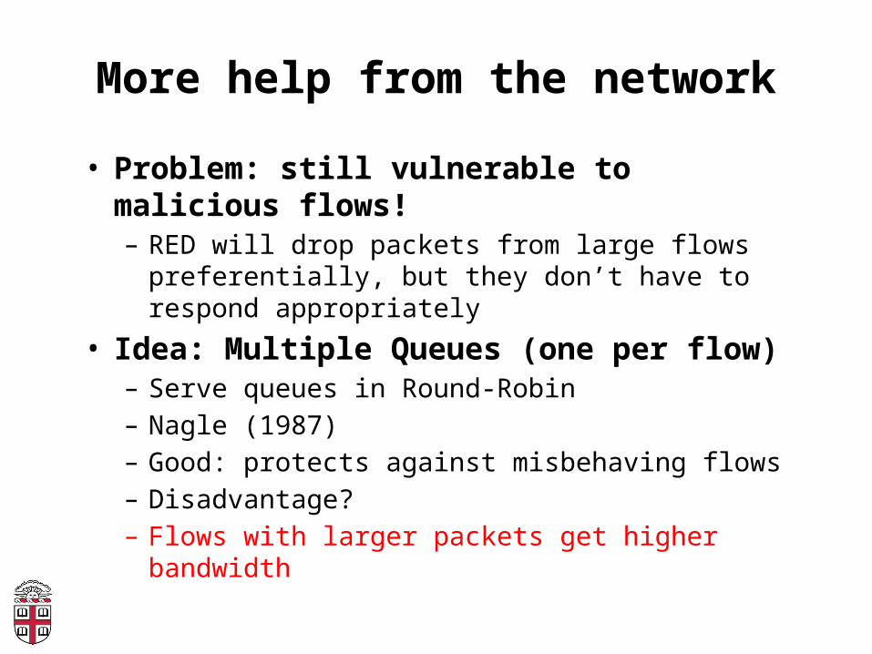
More help from the network

• Problem: still vulnerable to malicious flows!– RED will drop packets from large flows

preferentially, but they don’t have to respond appropriately

• Idea: Multiple Queues (one per flow)– Serve queues in Round-Robin– Nagle (1987)– Good: protects against misbehaving flows– Disadvantage?– Flows with larger packets get higher

bandwidth

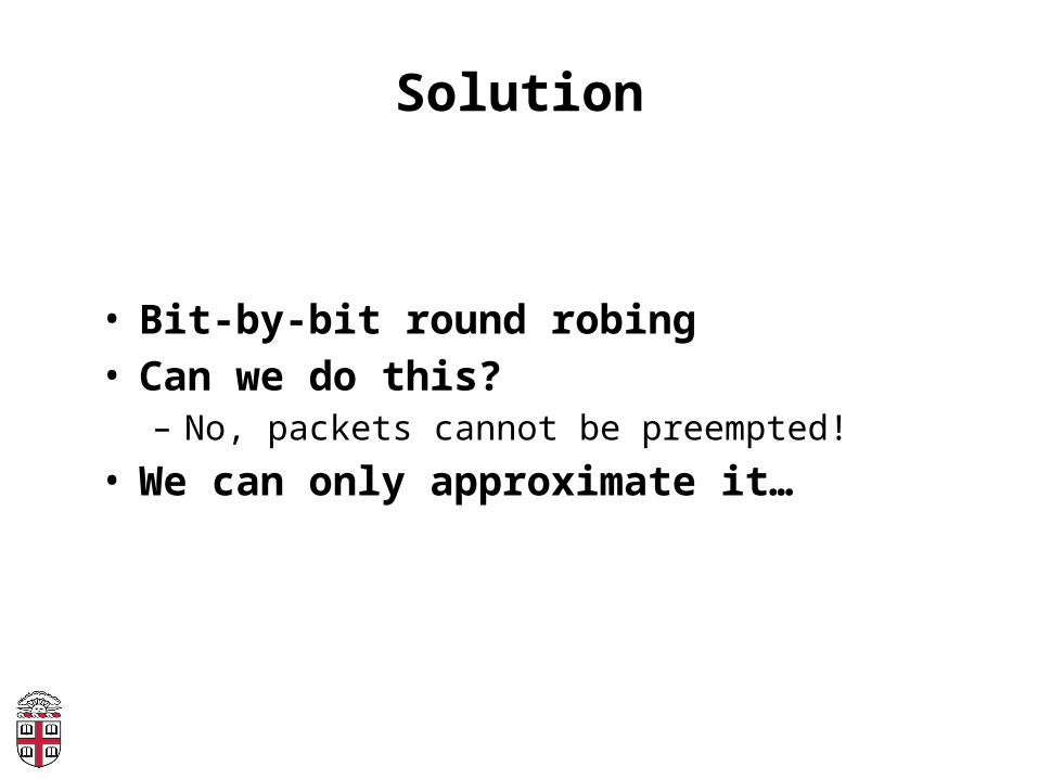
Solution

• Bit-by-bit round robing• Can we do this?

– No, packets cannot be preempted!

• We can only approximate it…

Fair Queueing

• Define a fluid flow system as one where flows are served bit-by-bit

• Simulate ff, and serve packets in the order in which they would finish in the ff system

• Each flow will receive exactly its fair share

Example

1 2 3 4 5

1 2 3 4

1 23

1 24

3 45

5 6

1 2 1 3 2 3 4 4

5 6

55 6

Flow 1(arrival traffic)

Flow 2(arrival traffic)

Servicein fluid flow system

Packetsystem

time

time

time

time

Implementing FQ• Suppose clock ticks with each bit

transmitted– (RR, among all active flows)

• Pi is the length of the packet

• Si is packet i’s start of transmission time

• Fi is packet i’s end of transmission time

• Fi = Si + Pi

• When does router start transmitting packet i?– If arrived before Fi-1, Si = Fi-1

– If no current packet for this flow, start when packet arrives (call this Ai): Si = Ai

• Thus, Fi = max(Fi-1,Ai) + Pi

Fair Queueing

• Across all flows– Calculate Fi for each packet that arrives on each flow

– Next packet to transmit is that with the lowest Fi

– Clock rate depends on the number of flows

• Advantages– Achieves max-min fairness, independent of sources– Work conserving

• Disadvantages– Requires non-trivial support from routers– Requires reliable identification of flows– Not perfect: can’t preempt packets

Fair Queueing Example

• 10Mbps link, 1 10Mbps UDP, 31 TCPs

FQ

0

0.2

0.4

0.6

0.8

1

1.2

1.4

1.6

1.8

2

1 4 7 10 13 16 19 22 25 28 31Flow Number

Thro

ughp

ut(M

bps)

RED

0

1

2

3

4

5

6

7

8

9

10

1 4 7 10 13 16 19 22 25 28 31Flow Number

Thro

ughp

ut(M

bps)

Big Picture

• Fair Queuing doesn’t eliminate congestion: just manages it

• You need both, ideally:– End-host congestion control to adapt– Router congestion control to provide

isolation