Embed Size (px)
Citation preview
CS675: Convex and Combinatorial OptimizationFall 2016
Combinatorial Problems as Linear and ConvexPrograms
Instructor: Shaddin Dughmi

Outline
1 Introduction
2 Shortest Path
3 Algorithms for Single-Source Shortest Path
4 Bipartite Matching
5 Total Unimodularity
6 Duality of Bipartite Matching and its Consequences
7 Spanning Trees
8 Flows
9 Max Cut

Combinatorial Vs Convex Optimization
In CS, discrete problems are traditionally viewed/analyzed usingdiscrete mathematics and combinatorics
Algorithms are combinatorial in nature (greedy, dynamicprogramming, divide and conquor, etc)
In OR and optimization community, these problems are oftenexpressed as continuous optimization problems
Usually linear programs, but increasingly more general convexprograms
Increasingly in recent history, it is becoming clear that combiningboth viewpoints is the way to go
Better algorithms (runtime, approximation)Structural insights (e.g. market clearing prices in matching markets)Unifying theories and general results (Matroids, submodularoptimization, constraint satisfaction)
Introduction 0/50
Discrete Problems as Linear Programs
The oldest examples of linear programs were discrete problemsDantzig’s original application was the problem of matching 70people to 70 jobs!
This is not surprising, since almost any finite family of discreteobjects can be encoded as a finite subset of Euclidean space
Convex hull of that set is a polytopeE.g. spanning trees, paths, cuts, TSP tours, assignments...
Introduction 1/50
Discrete Problems as Linear Programs
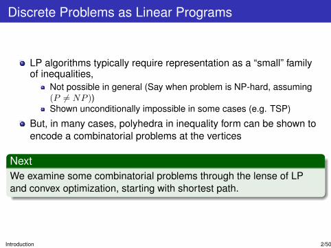
LP algorithms typically require representation as a “small” familyof inequalities,
Not possible in general (Say when problem is NP-hard, assuming(P 6= NP ))Shown unconditionally impossible in some cases (e.g. TSP)
But, in many cases, polyhedra in inequality form can be shown toencode a combinatorial problems at the vertices
NextWe examine some combinatorial problems through the lense of LPand convex optimization, starting with shortest path.
Introduction 2/50
Discrete Problems as Linear Programs
LP algorithms typically require representation as a “small” familyof inequalities,
Not possible in general (Say when problem is NP-hard, assuming(P 6= NP ))Shown unconditionally impossible in some cases (e.g. TSP)
But, in many cases, polyhedra in inequality form can be shown toencode a combinatorial problems at the vertices
NextWe examine some combinatorial problems through the lense of LPand convex optimization, starting with shortest path.
Introduction 2/50

Outline
1 Introduction
2 Shortest Path
3 Algorithms for Single-Source Shortest Path
4 Bipartite Matching
5 Total Unimodularity
6 Duality of Bipartite Matching and its Consequences
7 Spanning Trees
8 Flows
9 Max Cut
The Shortest Path Problem
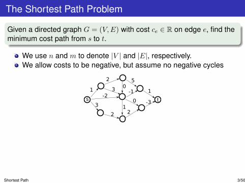
Given a directed graph G = (V,E) with cost ce ∈ R on edge e, find theminimum cost path from s to t.
We use n and m to denote |V | and |E|, respectively.We allow costs to be negative, but assume no negative cycles
s t
1
2
1
2
3
5
-2
30
0-1
2
-31
When costs are nonnegative, Dijkstra’s algorithm finds the shortestpath from s to every other node in time O(m+ n log n).
Using primal/dual paradigm, we will design a polynomial-time algorithmthat works when graph has negative edges but no negative cycles
Shortest Path 3/50

The Shortest Path Problem
Given a directed graph G = (V,E) with cost ce ∈ R on edge e, find theminimum cost path from s to t.
We use n and m to denote |V | and |E|, respectively.We allow costs to be negative, but assume no negative cycles
s t
1
2
1
2
3
5
-2
30
0-1
2
-31
When costs are nonnegative, Dijkstra’s algorithm finds the shortestpath from s to every other node in time O(m+ n log n).
Using primal/dual paradigm, we will design a polynomial-time algorithmthat works when graph has negative edges but no negative cycles
Shortest Path 3/50

Note: Negative Edges and Complexity
When the graph has no negative cycles, there is a shortest pathwhich is simpleWhen the graph has negative cycles, there may not be a shortestpath from s to t.In these cases, the algorithm we design can be modified to “failgracefully” by detecting such a cycle
Can be used to detect arbitrage opportunities in currency exchangenetworks
In the presence of negative cycles, finding the shortest simplepath is NP-hard (by reduction from Hamiltonian cycle)
Shortest Path 4/50
An LP Relaxation of Shortest Path
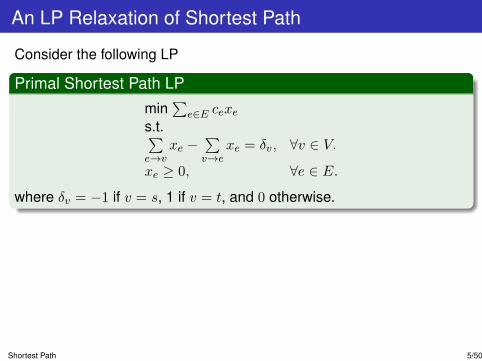
Consider the following LP
Primal Shortest Path LPmin
∑e∈E cexe
s.t.∑e→v
xe −∑v→e
xe = δv, ∀v ∈ V.
xe ≥ 0, ∀e ∈ E.
where δv = −1 if v = s, 1 if v = t, and 0 otherwise.
This is a relaxation of the shortest path problemIndicator vector xP of s− t path P is a feasible solution, with cost asgiven by the objectiveFractional feasible solutions may not correspond to paths
A-priori, it is conceivable that optimal value of LP is less thanlength of shortest path.
Shortest Path 5/50

An LP Relaxation of Shortest Path
Consider the following LP
Primal Shortest Path LPmin
∑e∈E cexe
s.t.∑e→v
xe −∑v→e
xe = δv, ∀v ∈ V.
xe ≥ 0, ∀e ∈ E.
where δv = −1 if v = s, 1 if v = t, and 0 otherwise.
This is a relaxation of the shortest path problemIndicator vector xP of s− t path P is a feasible solution, with cost asgiven by the objectiveFractional feasible solutions may not correspond to paths
A-priori, it is conceivable that optimal value of LP is less thanlength of shortest path.
Shortest Path 5/50
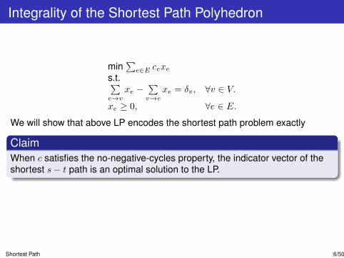
Integrality of the Shortest Path Polyhedron
min∑e∈E cexe
s.t.∑e→v
xe −∑v→e
xe = δv, ∀v ∈ V.
xe ≥ 0, ∀e ∈ E.
We will show that above LP encodes the shortest path problem exactly
ClaimWhen c satisfies the no-negative-cycles property, the indicator vector of theshortest s− t path is an optimal solution to the LP.
Shortest Path 6/50
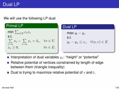
Dual LP
We will use the following LP dual
Primal LP
min∑
e∈E cexes.t.∑e→v
xe −∑v→e
xe = δv, ∀v ∈ V.
xe ≥ 0, ∀e ∈ E.
Dual LPmax yt − yss.t.yv − yu ≤ ce, ∀(u, v) ∈ E.
Interpretation of dual variables yv: “height” or “potential”Relative potential of vertices constrained by length of edgebetween them (triangle inequality)Dual is trying to maximize relative potential of s and t,
Shortest Path 7/50

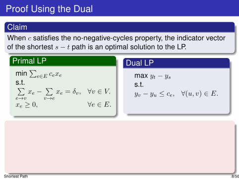
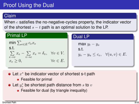
Proof Using the Dual
ClaimWhen c satisfies the no-negative-cycles property, the indicator vectorof the shortest s− t path is an optimal solution to the LP.
Primal LPmin
∑e∈E cexe
s.t.∑e→v
xe −∑v→e
xe = δv, ∀v ∈ V.
xe ≥ 0, ∀e ∈ E.
Dual LPmax yt − yss.t.yv − yu ≤ ce, ∀(u, v) ∈ E.
Let x∗ be indicator vector of shortest s-t pathFeasible for primal
Let y∗v be shortest path distance from s to vFeasible for dual (by triangle inequality)∑
e cex∗e = y∗t − y∗s , so both x∗ and y∗ optimal.
Shortest Path 8/50
Proof Using the Dual
ClaimWhen c satisfies the no-negative-cycles property, the indicator vectorof the shortest s− t path is an optimal solution to the LP.
Primal LPmin
∑e∈E cexe
s.t.∑e→v
xe −∑v→e
xe = δv, ∀v ∈ V.
xe ≥ 0, ∀e ∈ E.
Dual LPmax yt − yss.t.yv − yu ≤ ce, ∀(u, v) ∈ E.
Let x∗ be indicator vector of shortest s-t pathFeasible for primal
Let y∗v be shortest path distance from s to vFeasible for dual (by triangle inequality)
∑e cex
∗e = y∗t − y∗s , so both x∗ and y∗ optimal.
Shortest Path 8/50

Proof Using the Dual
ClaimWhen c satisfies the no-negative-cycles property, the indicator vectorof the shortest s− t path is an optimal solution to the LP.
Primal LPmin
∑e∈E cexe
s.t.∑e→v
xe −∑v→e
xe = δv, ∀v ∈ V.
xe ≥ 0, ∀e ∈ E.
Dual LPmax yt − yss.t.yv − yu ≤ ce, ∀(u, v) ∈ E.
Let x∗ be indicator vector of shortest s-t pathFeasible for primal
Let y∗v be shortest path distance from s to vFeasible for dual (by triangle inequality)∑
e cex∗e = y∗t − y∗s , so both x∗ and y∗ optimal.
Shortest Path 8/50
Integrality of Polyhedra
A stronger statement is true:
Integrality of Shortest Path LPThe vertices of the polyhedral feasible region are precisely theindicator vectors of simple paths in G.
Implies that there always exists an optimal solution which is a pathwhenever LP is bounded and feasibleReduces computing shortest path in graphs with no negativecycles to finding optimal vertex of LP
Shortest Path 9/50
Integrality of Polyhedra
A stronger statement is true:
Integrality of Shortest Path LPThe vertices of the polyhedral feasible region are precisely theindicator vectors of simple paths in G.
Proof1 LP is bounded iff c satisfies no-negative-cycles
←: previous proof→: If c has a negative cycle, there are arbitrarily cheap “flows”along that cycle
2 Fact: For every LP vertex x there is objective c such that x isunique optimal. (Prove it!)
3 Since such a c satisfies no-negative-cycles property, our previousclaim shows that x is integral.
Shortest Path 9/50
Integrality of Polyhedra
A stronger statement is true:
Integrality of Shortest Path LPThe vertices of the polyhedral feasible region are precisely theindicator vectors of simple paths in G.
In general, the approach we took applies in many contexts: To show apolytope’s vertices integral, it suffices to show that there is an integraloptimal for any objective which admits an optimal solution.
Shortest Path 9/50

Outline
1 Introduction
2 Shortest Path
3 Algorithms for Single-Source Shortest Path
4 Bipartite Matching
5 Total Unimodularity
6 Duality of Bipartite Matching and its Consequences
7 Spanning Trees
8 Flows
9 Max Cut
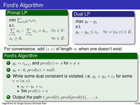
Ford’s AlgorithmPrimal LPmin
∑e∈E cexe
s.t.∑e→v
xe −∑v→e
xe = δv, ∀v ∈ V.
xe ≥ 0, ∀e ∈ E.
Dual LPmax yt − yss.t.yv − yu ≤ ce, ∀e = (u, v) ∈ E.
For convenience, add (s, v) of length∞ when one doesn’t exist.
Ford’s Algorithm1 yv = c(s,v) and pred(v)← s for v 6= s
2 ys ← 0, pred(s) = null.3 While some dual constraint is violated, i.e. yv > yu + ce for somee = (u, v)
yv ← yu + ceSet pred(v) = u
4 Output the path t, pred(t), pred(pred(t)), . . . , s.Algorithms for Single-Source Shortest Path 10/50

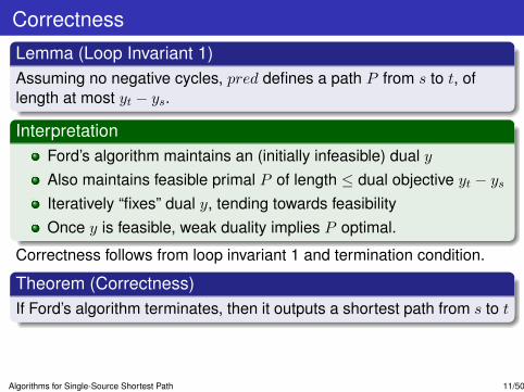
Correctness
Lemma (Loop Invariant 1)Assuming no negative cycles, pred defines a path P from s to t, oflength at most yt − ys.
InterpretationFord’s algorithm maintains an (initially infeasible) dual yAlso maintains feasible primal P of length ≤ dual objective yt − ysIteratively “fixes” dual y, tending towards feasibilityOnce y is feasible, weak duality implies P optimal.
Correctness follows from loop invariant 1 and termination condition.
Theorem (Correctness)If Ford’s algorithm terminates, then it outputs a shortest path from s to t
Algorithms of this form, that output a matching primal and dualsolution, are called Primal-Dual Algorithms.
Algorithms for Single-Source Shortest Path 11/50
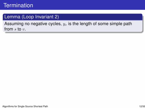
Termination
Lemma (Loop Invariant 2)Assuming no negative cycles, yv is the length of some simple pathfrom s to v.
Theorem (Termination)When the graph has no negative cycles, Ford’s algorithm terminates ina finite number of steps.
ProofThe graph has a finite number N of simple pathsBy loop invariant 2, every dual variable yv is the length of somesimple path.Dual variables are nonincreasing throughout algorithm, and onedecreases each iteration.There can be at most nN iterations.
Algorithms for Single-Source Shortest Path 12/50

Observation: Single sink shortest paths
Ford’s Algorithm1 yv = c(s,v) and pred(v)← s for v 6= s
2 ys ← 0, pred(s) = null.3 While some dual constraint is violated, i.e. yv > yu + ce for somee = (u, v)
yv ← yu + ceSet pred(v) = u
4 Output the path t, pred(t), pred(pred(t)), . . . , s.
ObservationAlgorithm does not depend on t till very last step. So essentially solvesthe single-source shortest path problem. i.e. finds shortest paths froms to all other vertices v.
Algorithms for Single-Source Shortest Path 13/50

Loop Invariant 1
We prove Loop Invariant 1 through two Lemmas
Lemma (Loop Invariant 1a)For every node w, we have yw − ypred(w) ≥ cpred(w),w
ProofFix wHolds at first iterationPreserved by Induction on iterations
If neither yw nor ypred(w) updated, nothing changes.If yw (and pred(w)) updated, then yw ← ypred(w) + cpred(w),w
ypred(w) updated, it only goes down, preserving inequality.
Algorithms for Single-Source Shortest Path 14/50
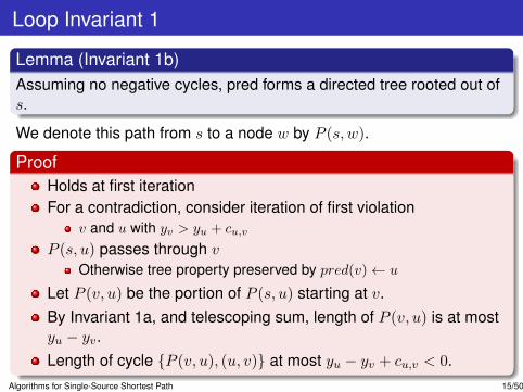
Loop Invariant 1
Lemma (Invariant 1b)Assuming no negative cycles, pred forms a directed tree rooted out ofs.
We denote this path from s to a node w by P (s, w).
ProofHolds at first iterationFor a contradiction, consider iteration of first violation
v and u with yv > yu + cu,v
P (s, u) passes through vOtherwise tree property preserved by pred(v)← u
Let P (v, u) be the portion of P (s, u) starting at v.By Invariant 1a, and telescoping sum, length of P (v, u) is at mostyu − yv.Length of cycle {P (v, u), (u, v)} at most yu − yv + cu,v < 0.
Algorithms for Single-Source Shortest Path 15/50

Summarizing Loop Invariant 1
Lemma (Invariant 1a)For every node w, we have yw − ypred(w) ≥ cpred(w),w.
By telescoping sum, can bound yw − ys when pred leads back to s
Lemma (Invariant 1b)Assuming no negative cycles, pred forms a directed tree rooted out ofs.
Implies that ys remains 0
Corollary (Loop Invariant 1)Assuming no negative cycles, pred defines a path P (s, w) from s toeach node w, of length at most yw − ys = yw.
Algorithms for Single-Source Shortest Path 16/50

Loop Invariant 2
Lemma (Loop Invariant 2)Assuming no negative cycles, yw is the length of some simple pathQ(s, w) from s to w, for all w.
Proof is technical, by induction, so we will skip. Instead, we will modifyFord’s algorithm to guarantee polynomial time termination.
Algorithms for Single-Source Shortest Path 17/50
Bellman-Ford Algorithm
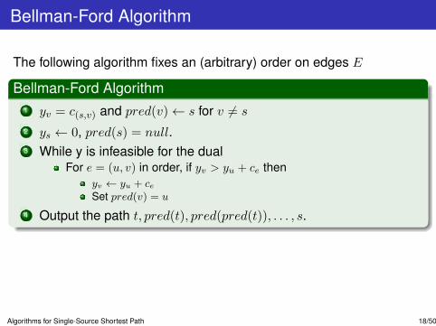
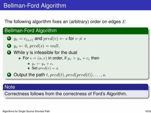
The following algorithm fixes an (arbitrary) order on edges E
Bellman-Ford Algorithm1 yv = c(s,v) and pred(v)← s for v 6= s
2 ys ← 0, pred(s) = null.3 While y is infeasible for the dual
For e = (u, v) in order, if yv > yu + ce thenyv ← yu + ceSet pred(v) = u
4 Output the path t, pred(t), pred(pred(t)), . . . , s.
NoteCorrectness follows from the correctness of Ford’s Algorithm.
Algorithms for Single-Source Shortest Path 18/50
Bellman-Ford Algorithm
The following algorithm fixes an (arbitrary) order on edges E
Bellman-Ford Algorithm1 yv = c(s,v) and pred(v)← s for v 6= s
2 ys ← 0, pred(s) = null.3 While y is infeasible for the dual
For e = (u, v) in order, if yv > yu + ce thenyv ← yu + ceSet pred(v) = u
4 Output the path t, pred(t), pred(pred(t)), . . . , s.
NoteCorrectness follows from the correctness of Ford’s Algorithm.
Algorithms for Single-Source Shortest Path 18/50

Runtime
TheoremBellman-Ford terminates after n− 1 scans through E, for a totalruntime of O(nm).
Follows immediately from the following Lemma
LemmaAfter k scans through E, vertices v with a shortest s− v pathconsisting of ≤ k edges are correctly labeled. (i.e., yv = distance(s, v))
Algorithms for Single-Source Shortest Path 19/50
Proof
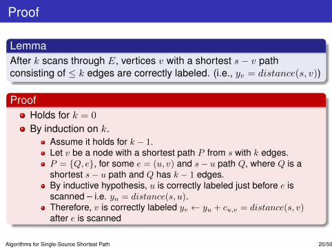
LemmaAfter k scans through E, vertices v with a shortest s− v pathconsisting of ≤ k edges are correctly labeled. (i.e., yv = distance(s, v))
ProofHolds for k = 0
By induction on k.Assume it holds for k − 1.Let v be a node with a shortest path P from s with k edges.P = {Q, e}, for some e = (u, v) and s− u path Q, where Q is ashortest s− u path and Q has k − 1 edges.By inductive hypothesis, u is correctly labeled just before e isscanned – i.e. yu = distance(s, u).Therefore, v is correctly labeled yv ← yu + cu,v = distance(s, v)after e is scanned
Algorithms for Single-Source Shortest Path 20/50
A Note on Negative Cycles
QuestionWhat if there are negative cycles? What does that say about LP? Whatabout Ford’s algorithm?
Algorithms for Single-Source Shortest Path 21/50

Outline
1 Introduction
2 Shortest Path
3 Algorithms for Single-Source Shortest Path
4 Bipartite Matching
5 Total Unimodularity
6 Duality of Bipartite Matching and its Consequences
7 Spanning Trees
8 Flows
9 Max Cut

The Max-Weight Bipartite Matching Problem
Given a bipartite graph G = (V,E), with V = L⋃R, and weights we on
edges e, find a maximum weight matching.
Matching: a set of edges covering each node at most onceWe use n and m to denote |V | and |E|, respectively.Equivalent to maximum weight / minimum cost perfect matching.
1 2
1.5
3
Our focus will be less on algorithms, and more on using polyhedralinterpretation to gain insights about a combinatorial problem.
Bipartite Matching 22/50

An LP Relaxation of Bipartite Matching
Bipartite Matching LP
max∑
e∈E wexes.t.∑e∈δ(v)
xe ≤ 1, ∀v ∈ V.
xe ≥ 0, ∀e ∈ E.
Feasible region is a polytope P (i.e. a bounded polyhedron)This is a relaxation of the bipartite matching problem
Integer points in P are the indicator vectors of matchings.
P ∩ Zm = {xM :M is a matching}
Bipartite Matching 23/50
Integrality of the Bipartite Matching Polytope
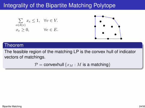
∑e∈δ(v)
xe ≤ 1, ∀v ∈ V.
xe ≥ 0, ∀e ∈ E.
TheoremThe feasible region of the matching LP is the convex hull of indicatorvectors of matchings.
P = convexhull {xM :M is a matching}
NoteThis is the strongest guarantee you could hope for of an LPrelaxation of a combinatorial problemSolving LP is equivalent to solving the combinatorial problemStronger guarantee than shortest path LP from last time
Bipartite Matching 24/50

Integrality of the Bipartite Matching Polytope
∑e∈δ(v)
xe ≤ 1, ∀v ∈ V.
xe ≥ 0, ∀e ∈ E.
TheoremThe feasible region of the matching LP is the convex hull of indicatorvectors of matchings.
P = convexhull {xM :M is a matching}
NoteThis is the strongest guarantee you could hope for of an LPrelaxation of a combinatorial problemSolving LP is equivalent to solving the combinatorial problemStronger guarantee than shortest path LP from last time
Bipartite Matching 24/50
Proof
1
1
0.7
0
0.3
0.6
0.1
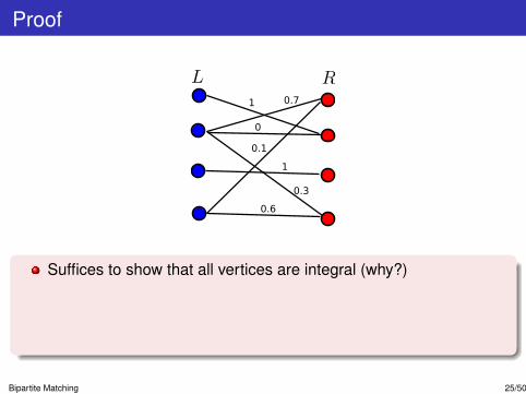
Suffices to show that all vertices are integral (why?)
Consider x ∈ P non-integral, we will show that x is not a vertex.Let H be the subgraph formed by edges with xe ∈ (0, 1)
H either contains a cycle, or else a maximal path which is simple.
Bipartite Matching 25/50

Proof
1
1
0.7
0
0.3
0.6
0.1
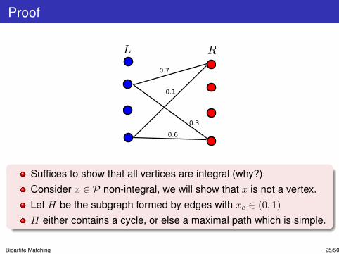
Suffices to show that all vertices are integral (why?)Consider x ∈ P non-integral, we will show that x is not a vertex.
Let H be the subgraph formed by edges with xe ∈ (0, 1)
H either contains a cycle, or else a maximal path which is simple.
Bipartite Matching 25/50

Proof
0.7
0.3
0.6
0.1
Suffices to show that all vertices are integral (why?)Consider x ∈ P non-integral, we will show that x is not a vertex.Let H be the subgraph formed by edges with xe ∈ (0, 1)
H either contains a cycle, or else a maximal path which is simple.
Bipartite Matching 25/50
Proof
0.7
0.3
0.6
0.1
Suffices to show that all vertices are integral (why?)Consider x ∈ P non-integral, we will show that x is not a vertex.Let H be the subgraph formed by edges with xe ∈ (0, 1)
H either contains a cycle, or else a maximal path which is simple.
Bipartite Matching 25/50
Proof
0.7
0.3
0.6
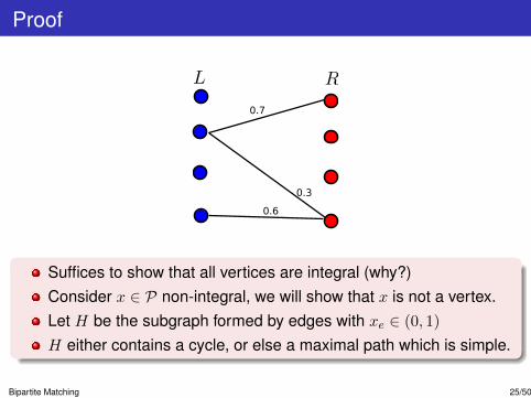
Suffices to show that all vertices are integral (why?)Consider x ∈ P non-integral, we will show that x is not a vertex.Let H be the subgraph formed by edges with xe ∈ (0, 1)
H either contains a cycle, or else a maximal path which is simple.
Bipartite Matching 25/50

Proof
0.7
0.3
0.6
0.1
Case 1: Cycle C
Let C = (e1, . . . , ek), with k evenThere is ε > 0 such that adding ±ε(+1,−1, . . . ,+1,−1) to xCpreserves feasibilityx is the midpoint of x+ ε(+1,−1, ...,+1,−1)C andx− ε(+1,−1, . . . ,+1,−1)C , so x is not a vertex.
Bipartite Matching 26/50
Proof
0.7
0.3
0.6
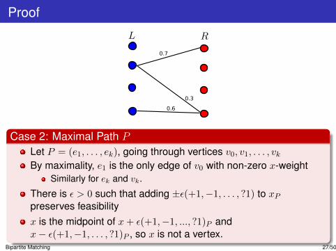
Case 2: Maximal Path P
Let P = (e1, . . . , ek), going through vertices v0, v1, . . . , vkBy maximality, e1 is the only edge of v0 with non-zero x-weight
Similarly for ek and vk.
There is ε > 0 such that adding ±ε(+1,−1, . . . , ?1) to xPpreserves feasibilityx is the midpoint of x+ ε(+1,−1, ..., ?1)P andx− ε(+1,−1, . . . , ?1)P , so x is not a vertex.
Bipartite Matching 27/50
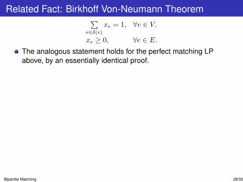
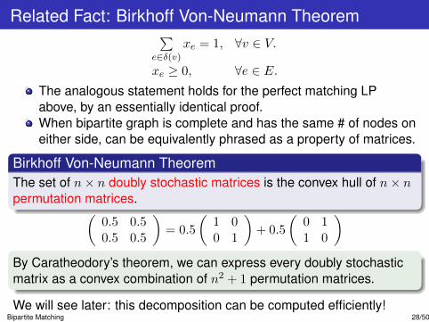
Related Fact: Birkhoff Von-Neumann Theorem∑e∈δ(v)
xe = 1, ∀v ∈ V.
xe ≥ 0, ∀e ∈ E.The analogous statement holds for the perfect matching LPabove, by an essentially identical proof.
When bipartite graph is complete and has the same # of nodes oneither side, can be equivalently phrased as a property of matrices.
Birkhoff Von-Neumann TheoremThe set of n× n doubly stochastic matrices is the convex hull of n× npermutation matrices.(
0.5 0.50.5 0.5
)= 0.5
(1 00 1
)+ 0.5
(0 11 0
)By Caratheodory’s theorem, we can express every doubly stochasticmatrix as a convex combination of n2 + 1 permutation matrices.
We will see later: this decomposition can be computed efficiently!
Bipartite Matching 28/50
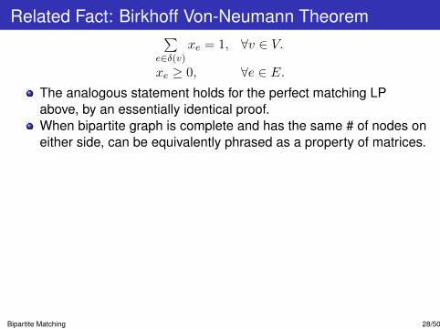
Related Fact: Birkhoff Von-Neumann Theorem∑e∈δ(v)
xe = 1, ∀v ∈ V.
xe ≥ 0, ∀e ∈ E.The analogous statement holds for the perfect matching LPabove, by an essentially identical proof.When bipartite graph is complete and has the same # of nodes oneither side, can be equivalently phrased as a property of matrices.
Birkhoff Von-Neumann TheoremThe set of n× n doubly stochastic matrices is the convex hull of n× npermutation matrices.(
0.5 0.50.5 0.5
)= 0.5
(1 00 1
)+ 0.5
(0 11 0
)By Caratheodory’s theorem, we can express every doubly stochasticmatrix as a convex combination of n2 + 1 permutation matrices.
We will see later: this decomposition can be computed efficiently!
Bipartite Matching 28/50
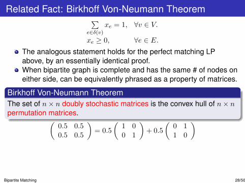
Related Fact: Birkhoff Von-Neumann Theorem∑e∈δ(v)
xe = 1, ∀v ∈ V.
xe ≥ 0, ∀e ∈ E.The analogous statement holds for the perfect matching LPabove, by an essentially identical proof.When bipartite graph is complete and has the same # of nodes oneither side, can be equivalently phrased as a property of matrices.
Birkhoff Von-Neumann TheoremThe set of n× n doubly stochastic matrices is the convex hull of n× npermutation matrices.(
0.5 0.50.5 0.5
)= 0.5
(1 00 1
)+ 0.5
(0 11 0
)
By Caratheodory’s theorem, we can express every doubly stochasticmatrix as a convex combination of n2 + 1 permutation matrices.
We will see later: this decomposition can be computed efficiently!
Bipartite Matching 28/50
Related Fact: Birkhoff Von-Neumann Theorem∑e∈δ(v)
xe = 1, ∀v ∈ V.
xe ≥ 0, ∀e ∈ E.The analogous statement holds for the perfect matching LPabove, by an essentially identical proof.When bipartite graph is complete and has the same # of nodes oneither side, can be equivalently phrased as a property of matrices.
Birkhoff Von-Neumann TheoremThe set of n× n doubly stochastic matrices is the convex hull of n× npermutation matrices.(
0.5 0.50.5 0.5
)= 0.5
(1 00 1
)+ 0.5
(0 11 0
)By Caratheodory’s theorem, we can express every doubly stochasticmatrix as a convex combination of n2 + 1 permutation matrices.
We will see later: this decomposition can be computed efficiently!Bipartite Matching 28/50

Outline
1 Introduction
2 Shortest Path
3 Algorithms for Single-Source Shortest Path
4 Bipartite Matching
5 Total Unimodularity
6 Duality of Bipartite Matching and its Consequences
7 Spanning Trees
8 Flows
9 Max Cut
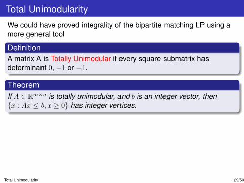
Total Unimodularity
We could have proved integrality of the bipartite matching LP using amore general tool
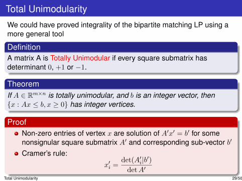
DefinitionA matrix A is Totally Unimodular if every square submatrix hasdeterminant 0, +1 or −1.
TheoremIf A ∈ Rm×n is totally unimodular, and b is an integer vector, then{x : Ax ≤ b, x ≥ 0} has integer vertices.
ProofNon-zero entries of vertex x are solution of A′x′ = b′ for somenonsignular square submatrix A′ and corresponding sub-vector b′
Cramer’s rule:
x′i =det(A′i|b′)detA′
Total Unimodularity 29/50
Total Unimodularity
We could have proved integrality of the bipartite matching LP using amore general tool
DefinitionA matrix A is Totally Unimodular if every square submatrix hasdeterminant 0, +1 or −1.
TheoremIf A ∈ Rm×n is totally unimodular, and b is an integer vector, then{x : Ax ≤ b, x ≥ 0} has integer vertices.
ProofNon-zero entries of vertex x are solution of A′x′ = b′ for somenonsignular square submatrix A′ and corresponding sub-vector b′
Cramer’s rule:
x′i =det(A′i|b′)detA′
Total Unimodularity 29/50

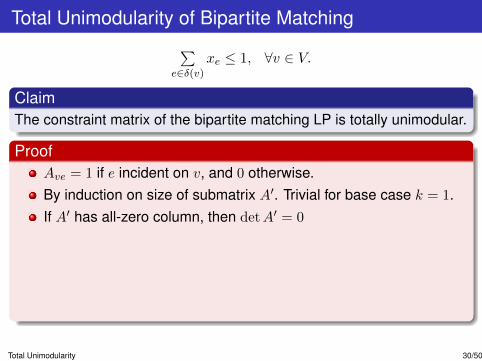
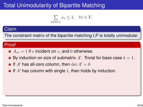
Total Unimodularity of Bipartite Matching∑
e∈δ(v)xe ≤ 1, ∀v ∈ V.
ClaimThe constraint matrix of the bipartite matching LP is totally unimodular.
ProofAve = 1 if e incident on v, and 0 otherwise.By induction on size of submatrix A′. Trivial for base case k = 1.If A′ has all-zero column, then detA′ = 0
If A′ has column with single 1, then holds by induction.If all columns of A′ have two 1’s,
Partition rows (vertices) into L and RSum of rows L is (1, 1, . . . , 1), similarly for RA′ is singular, so detA′ = 0.
Total Unimodularity 30/50

Total Unimodularity of Bipartite Matching∑
e∈δ(v)xe ≤ 1, ∀v ∈ V.
ClaimThe constraint matrix of the bipartite matching LP is totally unimodular.
ProofAve = 1 if e incident on v, and 0 otherwise.By induction on size of submatrix A′. Trivial for base case k = 1.
If A′ has all-zero column, then detA′ = 0
If A′ has column with single 1, then holds by induction.If all columns of A′ have two 1’s,
Partition rows (vertices) into L and RSum of rows L is (1, 1, . . . , 1), similarly for RA′ is singular, so detA′ = 0.
Total Unimodularity 30/50
Total Unimodularity of Bipartite Matching∑
e∈δ(v)xe ≤ 1, ∀v ∈ V.
ClaimThe constraint matrix of the bipartite matching LP is totally unimodular.
ProofAve = 1 if e incident on v, and 0 otherwise.By induction on size of submatrix A′. Trivial for base case k = 1.If A′ has all-zero column, then detA′ = 0
If A′ has column with single 1, then holds by induction.If all columns of A′ have two 1’s,
Partition rows (vertices) into L and RSum of rows L is (1, 1, . . . , 1), similarly for RA′ is singular, so detA′ = 0.
Total Unimodularity 30/50
Total Unimodularity of Bipartite Matching∑
e∈δ(v)xe ≤ 1, ∀v ∈ V.
ClaimThe constraint matrix of the bipartite matching LP is totally unimodular.
ProofAve = 1 if e incident on v, and 0 otherwise.By induction on size of submatrix A′. Trivial for base case k = 1.If A′ has all-zero column, then detA′ = 0
If A′ has column with single 1, then holds by induction.
If all columns of A′ have two 1’s,Partition rows (vertices) into L and RSum of rows L is (1, 1, . . . , 1), similarly for RA′ is singular, so detA′ = 0.
Total Unimodularity 30/50

Total Unimodularity of Bipartite Matching∑
e∈δ(v)xe ≤ 1, ∀v ∈ V.
ClaimThe constraint matrix of the bipartite matching LP is totally unimodular.
ProofAve = 1 if e incident on v, and 0 otherwise.By induction on size of submatrix A′. Trivial for base case k = 1.If A′ has all-zero column, then detA′ = 0
If A′ has column with single 1, then holds by induction.If all columns of A′ have two 1’s,
Partition rows (vertices) into L and RSum of rows L is (1, 1, . . . , 1), similarly for RA′ is singular, so detA′ = 0.
Total Unimodularity 30/50

Outline
1 Introduction
2 Shortest Path
3 Algorithms for Single-Source Shortest Path
4 Bipartite Matching
5 Total Unimodularity
6 Duality of Bipartite Matching and its Consequences
7 Spanning Trees
8 Flows
9 Max Cut
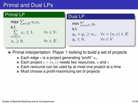
Primal and Dual LPs
Primal LPmax
∑e∈E wexe
s.t.∑e∈δ(v)
xe ≤ 1, ∀v ∈ V.
xe ≥ 0, ∀e ∈ E.
Dual LPmin
∑v∈V yv
s.t.yu + yv ≥ we, ∀e = (u, v) ∈ E.yv � 0, ∀v ∈ V.
Primal interpertation: Player 1 looking to build a set of projectsEach edge e is a project generating “profit” weEach project e = (u, v) needs two resources, u and vEach resource can be used by at most one project at a timeMust choose a profit-maximizing set of projects
Dual interpertation: Player 2 looking to buy resourcesOffer a price yv for each resource.Prices should incentivize player 1 to sell resourcesWant to pay as little as possible.
Duality of Bipartite Matching and its Consequences 31/50
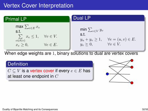
Vertex Cover Interpretation
Primal LPmax
∑e∈E xe
s.t.∑e∈δ(v)
xe ≤ 1, ∀v ∈ V.
xe ≥ 0, ∀e ∈ E.
Dual LP
min∑v∈V yv
s.t.yu + yv ≥ 1, ∀e = (u, v) ∈ E.yv � 0, ∀v ∈ V.
When edge weights are 1, binary solutions to dual are vertex covers
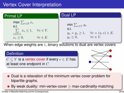
DefinitionC ⊆ V is a vertex cover if every e ∈ E hasat least one endpoint in C
Dual is a relaxation of the minimum vertex cover problem forbipartite graphs.By weak duality: min-vertex-cover ≥ max-cardinality-matching
Duality of Bipartite Matching and its Consequences 32/50
Vertex Cover Interpretation
Primal LPmax
∑e∈E xe
s.t.∑e∈δ(v)
xe ≤ 1, ∀v ∈ V.
xe ≥ 0, ∀e ∈ E.
Dual LP
min∑v∈V yv
s.t.yu + yv ≥ 1, ∀e = (u, v) ∈ E.yv � 0, ∀v ∈ V.
When edge weights are 1, binary solutions to dual are vertex covers
DefinitionC ⊆ V is a vertex cover if every e ∈ E hasat least one endpoint in C
Dual is a relaxation of the minimum vertex cover problem forbipartite graphs.By weak duality: min-vertex-cover ≥ max-cardinality-matching
Duality of Bipartite Matching and its Consequences 32/50
König’s Theorem
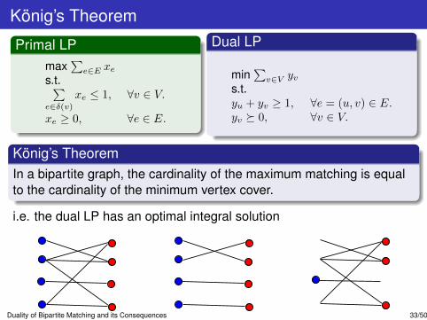
Primal LPmax
∑e∈E xe
s.t.∑e∈δ(v)
xe ≤ 1, ∀v ∈ V.
xe ≥ 0, ∀e ∈ E.
Dual LP
min∑v∈V yv
s.t.yu + yv ≥ 1, ∀e = (u, v) ∈ E.yv � 0, ∀v ∈ V.
König’s TheoremIn a bipartite graph, the cardinality of the maximum matching is equalto the cardinality of the minimum vertex cover.
i.e. the dual LP has an optimal integral solution
Duality of Bipartite Matching and its Consequences 33/50
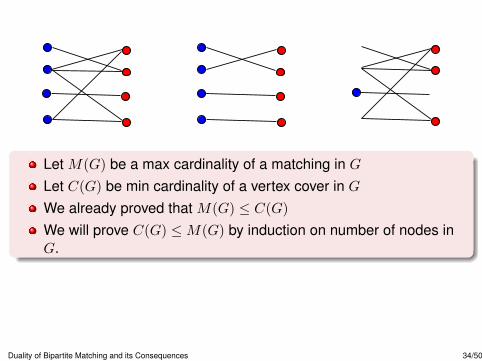
Let M(G) be a max cardinality of a matching in GLet C(G) be min cardinality of a vertex cover in GWe already proved that M(G) ≤ C(G)We will prove C(G) ≤M(G) by induction on number of nodes inG.
Note: Could have proved the same using total unimodularity
Duality of Bipartite Matching and its Consequences 34/50
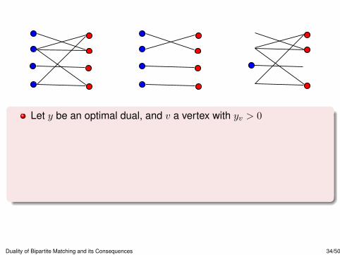
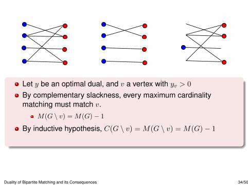
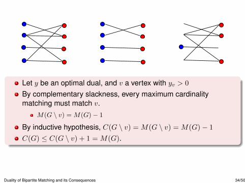
Let y be an optimal dual, and v a vertex with yv > 0
By complementary slackness, every maximum cardinalitymatching must match v.
M(G \ v) =M(G)− 1
By inductive hypothesis, C(G \ v) =M(G \ v) =M(G)− 1
C(G) ≤ C(G \ v) + 1 =M(G).
Note: Could have proved the same using total unimodularity
Duality of Bipartite Matching and its Consequences 34/50

Consequences of König’s Theorem
Vertex covers can serve as a certificate of optimality for bipartitematchings, and vice versa
Like maximum cardinality matching, minimum vertex cover inbipartite graphs can be formulated as an LP, and solved inpolynomial timeThe same is true for the maximum independent set problem inbipartite graphs.
C is a vertex cover iff V \ C is an independent set.
Duality of Bipartite Matching and its Consequences 35/50

Consequences of König’s Theorem
Vertex covers can serve as a certificate of optimality for bipartitematchings, and vice versaLike maximum cardinality matching, minimum vertex cover inbipartite graphs can be formulated as an LP, and solved inpolynomial time
The same is true for the maximum independent set problem inbipartite graphs.
C is a vertex cover iff V \ C is an independent set.
Duality of Bipartite Matching and its Consequences 35/50

Consequences of König’s Theorem
Vertex covers can serve as a certificate of optimality for bipartitematchings, and vice versaLike maximum cardinality matching, minimum vertex cover inbipartite graphs can be formulated as an LP, and solved inpolynomial timeThe same is true for the maximum independent set problem inbipartite graphs.
C is a vertex cover iff V \ C is an independent set.
Duality of Bipartite Matching and its Consequences 35/50

Outline
1 Introduction
2 Shortest Path
3 Algorithms for Single-Source Shortest Path
4 Bipartite Matching
5 Total Unimodularity
6 Duality of Bipartite Matching and its Consequences
7 Spanning Trees
8 Flows
9 Max Cut
The Minimum Cost Spanning Tree Problem
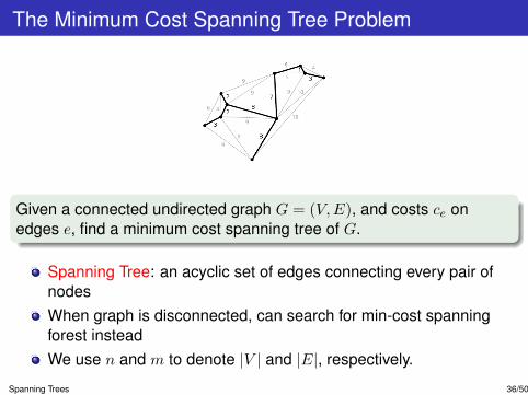
Given a connected undirected graph G = (V,E), and costs ce onedges e, find a minimum cost spanning tree of G.
Spanning Tree: an acyclic set of edges connecting every pair ofnodesWhen graph is disconnected, can search for min-cost spanningforest insteadWe use n and m to denote |V | and |E|, respectively.
Spanning Trees 36/50
Kruskal’s Algorithm
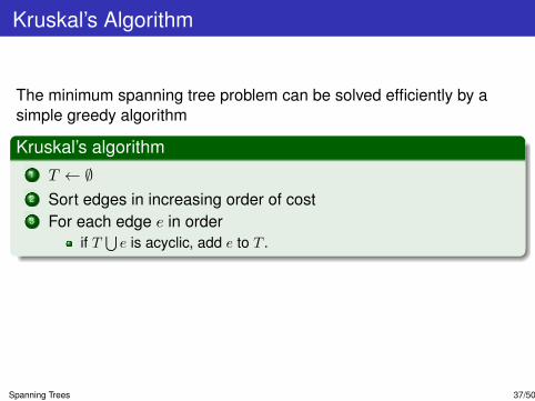
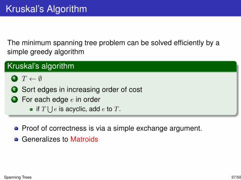
The minimum spanning tree problem can be solved efficiently by asimple greedy algorithm
Kruskal’s algorithm1 T ← ∅2 Sort edges in increasing order of cost3 For each edge e in order
if T⋃e is acyclic, add e to T .
Proof of correctness is via a simple exchange argument.Generalizes to Matroids
Spanning Trees 37/50
Kruskal’s Algorithm
The minimum spanning tree problem can be solved efficiently by asimple greedy algorithm
Kruskal’s algorithm1 T ← ∅2 Sort edges in increasing order of cost3 For each edge e in order
if T⋃e is acyclic, add e to T .
Proof of correctness is via a simple exchange argument.Generalizes to Matroids
Spanning Trees 37/50

MST Linear Program
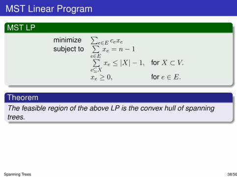
MST LPminimize
∑e∈E cexe
subject to∑e∈E
xe = n− 1∑e⊆X
xe ≤ |X| − 1, for X ⊂ V.
xe ≥ 0, for e ∈ E.
TheoremThe feasible region of the above LP is the convex hull of spanningtrees.
Proof by finding a dual solution with cost matching the output ofKruskal’s algorithm (on board)Generalizes to MatroidsNote: this LP has an exponential (in n) number of constraints
Spanning Trees 38/50
MST Linear Program
MST LPminimize
∑e∈E cexe
subject to∑e∈E
xe = n− 1∑e⊆X
xe ≤ |X| − 1, for X ⊂ V.
xe ≥ 0, for e ∈ E.
TheoremThe feasible region of the above LP is the convex hull of spanningtrees.
Proof by finding a dual solution with cost matching the output ofKruskal’s algorithm (on board)Generalizes to MatroidsNote: this LP has an exponential (in n) number of constraints
Spanning Trees 38/50

MST Linear Program
MST LPminimize
∑e∈E cexe
subject to∑e∈E
xe = n− 1∑e⊆X
xe ≤ |X| − 1, for X ⊂ V.
xe ≥ 0, for e ∈ E.
TheoremThe feasible region of the above LP is the convex hull of spanningtrees.
Proof by finding a dual solution with cost matching the output ofKruskal’s algorithm (on board)
Generalizes to MatroidsNote: this LP has an exponential (in n) number of constraints
Spanning Trees 38/50

MST Linear Program
MST LPminimize
∑e∈E cexe
subject to∑e∈E
xe = n− 1∑e⊆X
xe ≤ |X| − 1, for X ⊂ V.
xe ≥ 0, for e ∈ E.
TheoremThe feasible region of the above LP is the convex hull of spanningtrees.
Proof by finding a dual solution with cost matching the output ofKruskal’s algorithm (on board)Generalizes to Matroids
Note: this LP has an exponential (in n) number of constraints
Spanning Trees 38/50

MST Linear Program
MST LPminimize
∑e∈E cexe
subject to∑e∈E
xe = n− 1∑e⊆X
xe ≤ |X| − 1, for X ⊂ V.
xe ≥ 0, for e ∈ E.
TheoremThe feasible region of the above LP is the convex hull of spanningtrees.
Proof by finding a dual solution with cost matching the output ofKruskal’s algorithm (on board)Generalizes to MatroidsNote: this LP has an exponential (in n) number of constraints
Spanning Trees 38/50
Solving the MST Linear Program
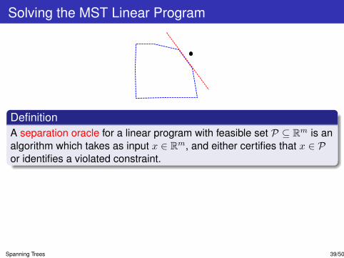
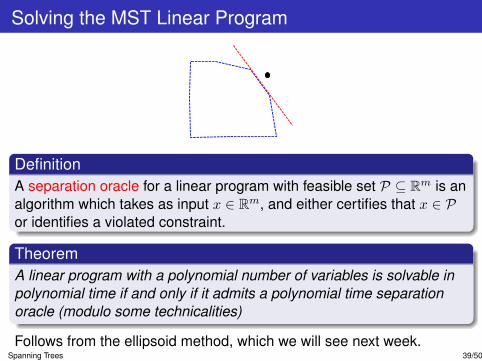
DefinitionA separation oracle for a linear program with feasible set P ⊆ Rm is analgorithm which takes as input x ∈ Rm, and either certifies that x ∈ Por identifies a violated constraint.
TheoremA linear program with a polynomial number of variables is solvable inpolynomial time if and only if it admits a polynomial time separationoracle (modulo some technicalities)
Follows from the ellipsoid method, which we will see next week.
Spanning Trees 39/50
Solving the MST Linear Program
DefinitionA separation oracle for a linear program with feasible set P ⊆ Rm is analgorithm which takes as input x ∈ Rm, and either certifies that x ∈ Por identifies a violated constraint.
TheoremA linear program with a polynomial number of variables is solvable inpolynomial time if and only if it admits a polynomial time separationoracle (modulo some technicalities)
Follows from the ellipsoid method, which we will see next week.Spanning Trees 39/50
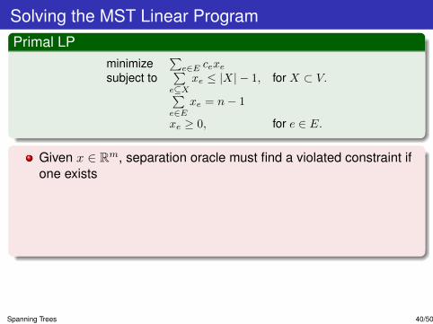
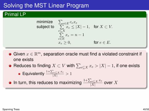
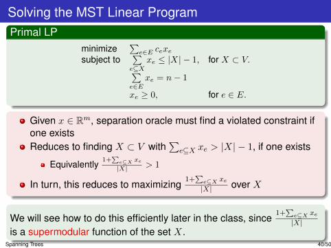
Solving the MST Linear ProgramPrimal LP
minimize∑e∈E cexe
subject to∑e⊆X
xe ≤ |X| − 1, for X ⊂ V.∑e∈E
xe = n− 1
xe ≥ 0, for e ∈ E.
Given x ∈ Rm, separation oracle must find a violated constraint ifone exists
Reduces to finding X ⊂ V with∑
e⊆X xe > |X| − 1, if one exists
Equivalently1+
∑e⊆X xe
|X| > 1
In turn, this reduces to maximizing1+
∑e⊆X xe
|X| over X
We will see how to do this efficiently later in the class, since1+
∑e⊆X xe
|X|is a supermodular function of the set X.
Spanning Trees 40/50

Solving the MST Linear ProgramPrimal LP
minimize∑e∈E cexe
subject to∑e⊆X
xe ≤ |X| − 1, for X ⊂ V.∑e∈E
xe = n− 1
xe ≥ 0, for e ∈ E.
Given x ∈ Rm, separation oracle must find a violated constraint ifone existsReduces to finding X ⊂ V with
∑e⊆X xe > |X| − 1, if one exists
Equivalently1+
∑e⊆X xe
|X| > 1
In turn, this reduces to maximizing1+
∑e⊆X xe
|X| over X
We will see how to do this efficiently later in the class, since1+
∑e⊆X xe
|X|is a supermodular function of the set X.
Spanning Trees 40/50

Application of Fractional Spanning Trees
The LP formulation of spanning trees has many applicationsWe will look at one contrived yet simple application that shows theflexibility enabled by polyhedral formulation
Fault-Tolerant MSTYour tree is an overlay network on the internet used to transmitdataA hacker is looking to attack your tree, by knocking off one of theedges of the graphYou can foil the hacker by choosing a random treeThe hacker knows the algorithm you use, but not your randomcoins
Spanning Trees 41/50
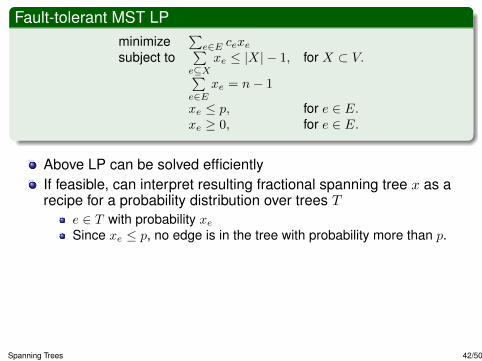
Fault-tolerant MST LPminimize
∑e∈E cexe
subject to∑e⊆X
xe ≤ |X| − 1, for X ⊂ V.∑e∈E
xe = n− 1
xe ≤ p, for e ∈ E.xe ≥ 0, for e ∈ E.
Above LP can be solved efficientlyIf feasible, can interpret resulting fractional spanning tree x as arecipe for a probability distribution over trees T
e ∈ T with probability xeSince xe ≤ p, no edge is in the tree with probability more than p.
Given feasible solution x, such a probability distribution exists!x is in the (original) MST polytopeCaratheodory’s theorem: x is a convex combination of m+ 1vertices of MST polytopeBy integrality of MST polytope: x is the “expectation” of a probabilitydistribution over spanning trees.
Consequence of Ellipsoid algorithm: can compute such adecomposition of x efficiently!
Spanning Trees 42/50

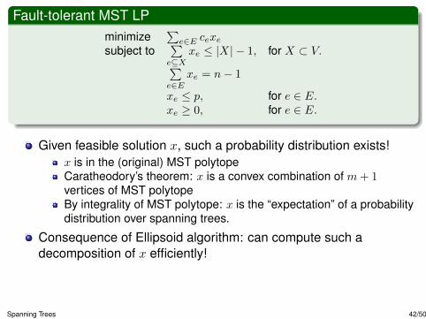
Fault-tolerant MST LPminimize
∑e∈E cexe
subject to∑e⊆X
xe ≤ |X| − 1, for X ⊂ V.∑e∈E
xe = n− 1
xe ≤ p, for e ∈ E.xe ≥ 0, for e ∈ E.
Given feasible solution x, such a probability distribution exists!
x is in the (original) MST polytopeCaratheodory’s theorem: x is a convex combination of m+ 1vertices of MST polytopeBy integrality of MST polytope: x is the “expectation” of a probabilitydistribution over spanning trees.
Consequence of Ellipsoid algorithm: can compute such adecomposition of x efficiently!
Spanning Trees 42/50

Fault-tolerant MST LPminimize
∑e∈E cexe
subject to∑e⊆X
xe ≤ |X| − 1, for X ⊂ V.∑e∈E
xe = n− 1
xe ≤ p, for e ∈ E.xe ≥ 0, for e ∈ E.
Given feasible solution x, such a probability distribution exists!x is in the (original) MST polytopeCaratheodory’s theorem: x is a convex combination of m+ 1vertices of MST polytopeBy integrality of MST polytope: x is the “expectation” of a probabilitydistribution over spanning trees.
Consequence of Ellipsoid algorithm: can compute such adecomposition of x efficiently!
Spanning Trees 42/50

Outline
1 Introduction
2 Shortest Path
3 Algorithms for Single-Source Shortest Path
4 Bipartite Matching
5 Total Unimodularity
6 Duality of Bipartite Matching and its Consequences
7 Spanning Trees
8 Flows
9 Max Cut
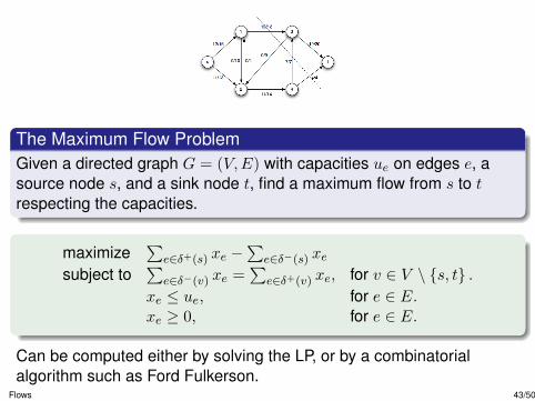
The Maximum Flow ProblemGiven a directed graph G = (V,E) with capacities ue on edges e, asource node s, and a sink node t, find a maximum flow from s to trespecting the capacities.
maximize∑
e∈δ+(s) xe −∑
e∈δ−(s) xesubject to
∑e∈δ−(v) xe =
∑e∈δ+(v) xe, for v ∈ V \ {s, t} .
xe ≤ ue, for e ∈ E.xe ≥ 0, for e ∈ E.
Can be computed either by solving the LP, or by a combinatorialalgorithm such as Ford Fulkerson.
Flows 43/50

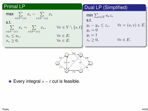
Primal LPmax
∑e∈δ+(s)
xe −∑
e∈δ−(s)
xe
s.t.∑e∈δ−(v)
xe =∑
e∈δ+(v)
xe, ∀v ∈ V \ {s, t} .
xe ≤ ue, ∀e ∈ E.xe ≥ 0, ∀e ∈ E.
Dual LP (Simplified)min
∑e∈E ueze
s.t.yv − yu ≤ ze, ∀e = (u, v) ∈ E.ys = 0yt = 1ze ≥ 0, ∀e ∈ E.
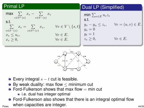
Dual solution describes fraction ze of each edge to fractionally cut
Dual constraints require that at least 1 edge is cut on every pathfrom s to t.∑
(u,v)∈P zuv ≥∑
(u,v)∈P yv − yu = yt − ys = 1
Every integral s− t cut is feasible.By weak duality: max flow ≤ minimum cutFord-Fulkerson shows that max flow = min cut
i.e. dual has integer optimalFord-Fulkerson also shows that there is an integral optimal flowwhen capacities are integer.
Flows 44/50

Primal LPmax
∑e∈δ+(s)
xe −∑
e∈δ−(s)
xe
s.t.∑e∈δ−(v)
xe =∑
e∈δ+(v)
xe, ∀v ∈ V \ {s, t} .
xe ≤ ue, ∀e ∈ E.xe ≥ 0, ∀e ∈ E.
Dual LP (Simplified)min
∑e∈E ueze
s.t.yv − yu ≤ ze, ∀e = (u, v) ∈ E.ys = 0yt = 1ze ≥ 0, ∀e ∈ E.
Dual solution describes fraction ze of each edge to fractionally cutDual constraints require that at least 1 edge is cut on every pathfrom s to t.∑
(u,v)∈P zuv ≥∑
(u,v)∈P yv − yu = yt − ys = 1
Every integral s− t cut is feasible.By weak duality: max flow ≤ minimum cutFord-Fulkerson shows that max flow = min cut
i.e. dual has integer optimalFord-Fulkerson also shows that there is an integral optimal flowwhen capacities are integer.
Flows 44/50
Primal LPmax
∑e∈δ+(s)
xe −∑
e∈δ−(s)
xe
s.t.∑e∈δ−(v)
xe =∑
e∈δ+(v)
xe, ∀v ∈ V \ {s, t} .
xe ≤ ue, ∀e ∈ E.xe ≥ 0, ∀e ∈ E.
Dual LP (Simplified)min
∑e∈E ueze
s.t.yv − yu ≤ ze, ∀e = (u, v) ∈ E.ys = 0yt = 1ze ≥ 0, ∀e ∈ E.
Every integral s− t cut is feasible.
By weak duality: max flow ≤ minimum cutFord-Fulkerson shows that max flow = min cut
i.e. dual has integer optimalFord-Fulkerson also shows that there is an integral optimal flowwhen capacities are integer.
Flows 44/50

Primal LPmax
∑e∈δ+(s)
xe −∑
e∈δ−(s)
xe
s.t.∑e∈δ−(v)
xe =∑
e∈δ+(v)
xe, ∀v ∈ V \ {s, t} .
xe ≤ ue, ∀e ∈ E.xe ≥ 0, ∀e ∈ E.
Dual LP (Simplified)min
∑e∈E ueze
s.t.yv − yu ≤ ze, ∀e = (u, v) ∈ E.ys = 0yt = 1ze ≥ 0, ∀e ∈ E.
Every integral s− t cut is feasible.By weak duality: max flow ≤ minimum cut
Ford-Fulkerson shows that max flow = min cuti.e. dual has integer optimal
Ford-Fulkerson also shows that there is an integral optimal flowwhen capacities are integer.
Flows 44/50

Primal LPmax
∑e∈δ+(s)
xe −∑
e∈δ−(s)
xe
s.t.∑e∈δ−(v)
xe =∑
e∈δ+(v)
xe, ∀v ∈ V \ {s, t} .
xe ≤ ue, ∀e ∈ E.xe ≥ 0, ∀e ∈ E.
Dual LP (Simplified)min
∑e∈E ueze
s.t.yv − yu ≤ ze, ∀e = (u, v) ∈ E.ys = 0yt = 1ze ≥ 0, ∀e ∈ E.
Every integral s− t cut is feasible.By weak duality: max flow ≤ minimum cutFord-Fulkerson shows that max flow = min cut
i.e. dual has integer optimal
Ford-Fulkerson also shows that there is an integral optimal flowwhen capacities are integer.
Flows 44/50
Primal LPmax
∑e∈δ+(s)
xe −∑
e∈δ−(s)
xe
s.t.∑e∈δ−(v)
xe =∑
e∈δ+(v)
xe, ∀v ∈ V \ {s, t} .
xe ≤ ue, ∀e ∈ E.xe ≥ 0, ∀e ∈ E.
Dual LP (Simplified)min
∑e∈E ueze
s.t.yv − yu ≤ ze, ∀e = (u, v) ∈ E.ys = 0yt = 1ze ≥ 0, ∀e ∈ E.
Every integral s− t cut is feasible.By weak duality: max flow ≤ minimum cutFord-Fulkerson shows that max flow = min cut
i.e. dual has integer optimalFord-Fulkerson also shows that there is an integral optimal flowwhen capacities are integer.Flows 44/50
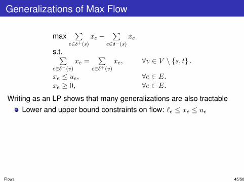
Generalizations of Max Flow
max∑
e∈δ+(s)
xe −∑
e∈δ−(s)
xe
s.t.∑e∈δ−(v)
xe =∑
e∈δ+(v)
xe, ∀v ∈ V \ {s, t} .
xe ≤ ue, ∀e ∈ E.xe ≥ 0, ∀e ∈ E.
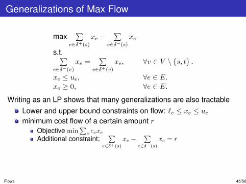
Writing as an LP shows that many generalizations are also tractable
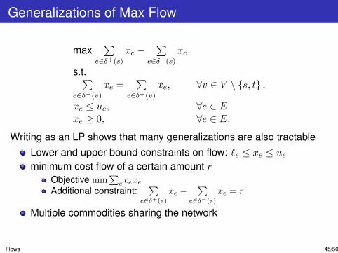
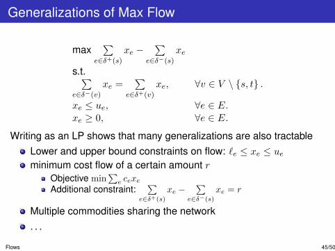
Lower and upper bound constraints on flow: `e ≤ xe ≤ ueminimum cost flow of a certain amount r
Objective min∑e cexe
Additional constraint:∑
e∈δ+(s)
xe −∑
e∈δ−(s)
xe = r
Multiple commodities sharing the network. . .
Flows 45/50
Generalizations of Max Flow
max∑
e∈δ+(s)
xe −∑
e∈δ−(s)
xe
s.t.∑e∈δ−(v)
xe =∑
e∈δ+(v)
xe, ∀v ∈ V \ {s, t} .
xe ≤ ue, ∀e ∈ E.xe ≥ 0, ∀e ∈ E.
Writing as an LP shows that many generalizations are also tractableLower and upper bound constraints on flow: `e ≤ xe ≤ ue
minimum cost flow of a certain amount rObjective min
∑e cexe
Additional constraint:∑
e∈δ+(s)
xe −∑
e∈δ−(s)
xe = r
Multiple commodities sharing the network. . .
Flows 45/50
Generalizations of Max Flow
max∑
e∈δ+(s)
xe −∑
e∈δ−(s)
xe
s.t.∑e∈δ−(v)
xe =∑
e∈δ+(v)
xe, ∀v ∈ V \ {s, t} .
xe ≤ ue, ∀e ∈ E.xe ≥ 0, ∀e ∈ E.
Writing as an LP shows that many generalizations are also tractableLower and upper bound constraints on flow: `e ≤ xe ≤ ueminimum cost flow of a certain amount r
Objective min∑e cexe
Additional constraint:∑
e∈δ+(s)
xe −∑
e∈δ−(s)
xe = r
Multiple commodities sharing the network. . .
Flows 45/50
Generalizations of Max Flow
max∑
e∈δ+(s)
xe −∑
e∈δ−(s)
xe
s.t.∑e∈δ−(v)
xe =∑
e∈δ+(v)
xe, ∀v ∈ V \ {s, t} .
xe ≤ ue, ∀e ∈ E.xe ≥ 0, ∀e ∈ E.
Writing as an LP shows that many generalizations are also tractableLower and upper bound constraints on flow: `e ≤ xe ≤ ueminimum cost flow of a certain amount r
Objective min∑e cexe
Additional constraint:∑
e∈δ+(s)
xe −∑
e∈δ−(s)
xe = r
Multiple commodities sharing the network
. . .
Flows 45/50
Generalizations of Max Flow
max∑
e∈δ+(s)
xe −∑
e∈δ−(s)
xe
s.t.∑e∈δ−(v)
xe =∑
e∈δ+(v)
xe, ∀v ∈ V \ {s, t} .
xe ≤ ue, ∀e ∈ E.xe ≥ 0, ∀e ∈ E.
Writing as an LP shows that many generalizations are also tractableLower and upper bound constraints on flow: `e ≤ xe ≤ ueminimum cost flow of a certain amount r
Objective min∑e cexe
Additional constraint:∑
e∈δ+(s)
xe −∑
e∈δ−(s)
xe = r
Multiple commodities sharing the network. . .
Flows 45/50
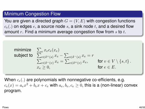
Minimum Congestion FlowYou are given a directed graph G = (V,E) with congestion functionsce(.) on edges e, a source node s, a sink node t, and a desired flowamount r. Find a minimum average congestion flow from s to t.
minimize∑
e xece(xe)subject to
∑e∈δ+(s) xe −
∑e∈δ−(s) xe = r∑
e∈δ−(v) xe =∑
e∈δ+(v) xe, for v ∈ V \ {s, t} .xe ≥ 0, for e ∈ E.
When ce(.) are polynomials with nonnegative co-efficients, e.g.ce(x) = aex
2 + bex+ ce with ae, be, ce ≥ 0, this is a (non-linear) convexprogram.
Flows 46/50

Outline
1 Introduction
2 Shortest Path
3 Algorithms for Single-Source Shortest Path
4 Bipartite Matching
5 Total Unimodularity
6 Duality of Bipartite Matching and its Consequences
7 Spanning Trees
8 Flows
9 Max Cut
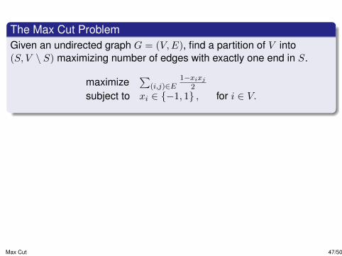
The Max Cut ProblemGiven an undirected graph G = (V,E), find a partition of V into(S, V \ S) maximizing number of edges with exactly one end in S.
maximize∑
(i,j)∈E1−xixj
2
subject to xi ∈ {−1, 1} , for i ∈ V.
Instead of requiring xi to be on the 1 dimensional sphere, we relax andpermit it to be in the n-dimensional sphere.
Vector Program relaxation
maximize∑
(i,j)∈E1−~vi·~vj
2
subject to ||~vi||2 = 1, for i ∈ V.~vi ∈ Rn, for i ∈ V.
Max Cut 47/50
SDP Relaxation
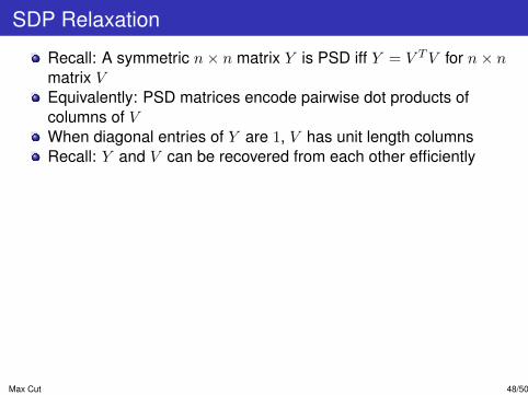
Recall: A symmetric n× n matrix Y is PSD iff Y = V TV for n× nmatrix VEquivalently: PSD matrices encode pairwise dot products ofcolumns of VWhen diagonal entries of Y are 1, V has unit length columnsRecall: Y and V can be recovered from each other efficiently
Vector Program relaxation
maximize∑
(i,j)∈E1−~vi·~vj
2
subject to ||~vi||2 = 1, for i ∈ V.~vi ∈ Rn, for i ∈ V.
SDP Relaxation
maximize∑
(i,j)∈E1−Yij
2
subject to Yii = 1, for i ∈ V.Y ∈ Sn+
Max Cut 48/50

SDP Relaxation
Recall: A symmetric n× n matrix Y is PSD iff Y = V TV for n× nmatrix VEquivalently: PSD matrices encode pairwise dot products ofcolumns of VWhen diagonal entries of Y are 1, V has unit length columnsRecall: Y and V can be recovered from each other efficiently
Vector Program relaxation
maximize∑
(i,j)∈E1−~vi·~vj
2
subject to ||~vi||2 = 1, for i ∈ V.~vi ∈ Rn, for i ∈ V.
SDP Relaxation
maximize∑
(i,j)∈E1−Yij
2
subject to Yii = 1, for i ∈ V.Y ∈ Sn+
Max Cut 48/50

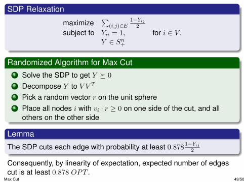
SDP Relaxation
maximize∑
(i,j)∈E1−Yij
2
subject to Yii = 1, for i ∈ V.Y ∈ Sn+
Randomized Algorithm for Max Cut1 Solve the SDP to get Y � 0
2 Decompose Y to V V T
3 Pick a random vector r on the unit sphere4 Place all nodes i with vi · r ≥ 0 on one side of the cut, and all
others on the other side
Lemma
The SDP cuts each edge with probability at least 0.8781−Yij2
Consequently, by linearity of expectation, expected number of edgescut is at least 0.878 OPT .
Max Cut 49/50
Lemma
The SDP cuts each edge with probability at least 0.8781−Yij2
We use the following fact
FactFor all angles θ ∈ [0, π],
θ
π≥ 0.878 · 1
2(1− cos(θ))
to prove the Lemma on the board.
Max Cut 50/50