1

CS6301 – PROGRAMMING & DATA STRUCTURES II

UNIT I

OBJECT ORIENTED PROGRAMMING FUNDAMENTALS

C++ Programming features - Data Abstraction - Encapsulation - class - object -

constructors – static members – constant members – member functions – pointers – references

- Role of this pointer –Storage classes – function as arguments.

Introduction:

The C++ programming language is based on the C language.

C++ (pronounced see plus plus) is a general purpose programming language that is

free-form and compiled.

It is regarded as an intermediate-level language, as it comprises both high-level and low-

level language features.

It provides imperative, object-oriented and generic programming features.

C++ is one of the most popular programming languages and is implemented on a wide

variety of hardware and operating system platforms.

As an efficient performance driven programming language it is used in systems

software, application software, device drivers, embedded software, high-performance

server and client applications, and entertainment software such as video games.

Various entities provide both open source and proprietary C++ compiler software,

including the FSF, LLVM, Microsoft and Intel.

It was developed by BjarneStroustrup starting in 1979 at Bell Labs, C++ was originally

named C with Classes, adding object-oriented features, such as classes, and other

enhancements to the C programming language.

The language was renamed C++ in 1983, as a pun involving the increment operator. It

began as enhancements to C, first adding classes, then virtual functions, operator

overloading, multiple inheritance, templates and exception handling, alongside changes

to the type system and other features.

It has influenced many other programming languages, including C#,[2]Java and newer

versions of C .

Operators and operator overloading

Operators that cannot be overloaded in C

Operator Symbol

Scope resolution operator ::

Conditional operator ?:

dot operator .

Member selection operator .*

"sizeof" operator sizeof

"typeid" operator typeid

2

C++ provides more than 35 operators, covering basic arithmetic, bit manipulation, indirection, comparisons, logical operations and others. Almost all operators can be overloadedfor user-defined types, with a few notable exceptions such as member access (. and

.*) as well as the conditional operator.

Memory management

C++ supports four types of memory management:

Static memory allocation. A static variable is assigned a value at compile-time, and allocated storage in a fixed location along with the executable code. These are declared with the "static" keyword (in the sense of static storage, not in the sense of declaring a class variable).

Automatic memory allocation. An automatic variable is simply declared with its class name, and storage is allocated on the stack when the value is assigned. The constructor is called when the declaration is executed, the destructor is called when the variable goes out of scope, and after the destructor the allocated memory is automatically freed.

Dynamic memory allocation. Storage can be dynamically allocated on the heap using manual memory management - normally calls to new and delete (though old-style C calls such as malloc() and free() are still supported).

With the use of a library, garbage collection is possible. The Boehm garbage collector is commonly used for this purpose.

The fine control over memory management is similar to C, but in contrast with languages that

intend to hide such details from the programmer, such as Java, Perl, PHP, and Ruby.

Templates

C++ templates enable generic programming.C++ supports both function and class templates. Templates may be parameterized by types, compile-time constants, and other templates.

Templates are implemented by instantiation at compile-time. To instantiate a template, compilers substitute specific arguments for a template's parameters to generate a concrete function or class instance.

Some substitutions are not possible; these are eliminated by an overload resolution policy described by the phrase "Substitution failure is not an error" (SFINAE).

Exception handling

Exception handling is a mechanism in C++ that is used to handle errors in a uniform manner and separately from the main body of a programme's source code.

Should an error occur, an exception is thrown (raised), which is then caught by an exception handler.

The code that might cause an exception to be thrown goes in a try block (is enclosed in try { and }) and the exceptions are handled in separate catch blocks.

Unknown errors can be caught by the handlers using catch(...) to catch all exceptions.Each try

block can have multiple handlers, allowing multiple different exceptions to be potentially caught.

3

Standard library

The C++ standard consists of two parts:

i) core language,

ii) C++ Standard Library;

which C++ programmers expect on every major implementation of C++, it includes vectors, lists, maps, algorithms (find, for_each, binary_search, random_shuffle, etc.), sets, queues, stacks, arrays, tuples, input/output facilities (iostream; reading from the console input, reading/writing from files), smart pointers for automatic memory management, regular expression support, multi-threading library, atomics support (allowing a variable to be read or written to be at most one thread at a time without any external synchronisation), time utilities (measurement, getting

current time, etc.), a system for converting error reporting that doesn't use C++ exceptions into

The Features of C++:

Objects

Classes

Data Abstraction

Data Encapsulation

Inheritance

Polymorphism

Message Passing Objects:

Objects are the basic run-time entities in an object oriented programming. They may represent a person, a place, abank account or any item that the program has to handle.

They may represent user-defined data such as vectors, timeand lists. Programming problem is analyzed in terms of objects and the nature of communication between them.Objects are the instances of the classes.

When a program is executed, the objects interact by sending messages to another. Each object contains data andcode to manipulate the data.

Objects can interact without having to know the details of each others data or code. It issufficient to know the type of message accepted, and the type of message accepted and the type of response returnedby the objects. Figure Shows the representation of an object.

4

Classes:

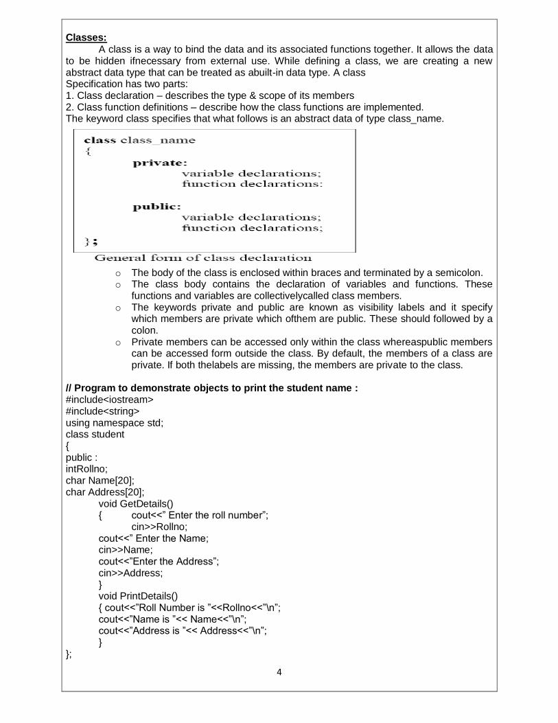
A class is a way to bind the data and its associated functions together. It allows the data to be hidden ifnecessary from external use. While defining a class, we are creating a new abstract data type that can be treated as abuilt-in data type. A class Specification has two parts: 1. Class declaration – describes the type & scope of its members 2. Class function definitions – describe how the class functions are implemented. The keyword class specifies that what follows is an abstract data of type class_name.

o The body of the class is enclosed within braces and terminated by a semicolon. o The class body contains the declaration of variables and functions. These

functions and variables are collectivelycalled class members. o The keywords private and public are known as visibility labels and it specify

which members are private which ofthem are public. These should followed by a colon.

o Private members can be accessed only within the class whereaspublic members can be accessed form outside the class. By default, the members of a class are private. If both thelabels are missing, the members are private to the class.

// Program to demonstrate objects to print the student name : #include<iostream> #include<string> using namespace std; class student { public : intRollno; char Name[20]; char Address[20];

void GetDetails() { cout<<” Enter the roll number”;

cin>>Rollno; cout<<” Enter the Name; cin>>Name; cout<<”Enter the Address”; cin>>Address; } void PrintDetails() { cout<<”Roll Number is ”<<Rollno<<”\n”; cout<<”Name is ”<< Name<<”\n”; cout<<”Address is ”<< Address<<”\n”; }

};

5

void main( ) { student Student1; Student1.GetDetails(); Student1.PrintDetails( ); } OutPut:Roll Number is:11

Name is:saran Address is: chennai Data Abstraction:

Abstraction represents the act of representing the essential features without including the background details orexplanations.

Classes use the concept of abstraction and are defined as a list of abstract attributes such as size,weight and cost and functions to operate on these attributes.

The attributes are called data members and functions arecalled member functions or methods. Abstraction is useful for the implementation purpose.

Actually the end userneed not worry about how the particular operation is implemented.

They should be facilitated only with theoperations and not with the implementation.For example, Applying break is an operation.

It is enough for the person who drives the car to know how pressure hehas to apply on the break pad rather than how the break system functions. The car mechanic will take care of thebreaking system.

Data Encapsulation

The wrapping up of data and functions into a single unit is known as encapsulation. It is the most striking feature ofthe class.

The data is not accessible to the outside world and only those functions which are wrapped in the class can access it.

These functions provide interface between the object‟s data and the program. This insulation of the data from direct access by the program is called data hiding or information hiding.

Inheritance:

It is the process by which objects of one class acquire the properties of objects of another class.

It supports theconcept of hierarchical classification. For example, the person „son‟ is a part of the class „father‟ which is again apart of the class „grandfather‟.

This concept provides the idea of reusability. This means that we can add additional features to an existing classwithout modifying it.

This is possible by a deriving a new class from an existing one. The new class will have the combined features of both the classes.

Types Of Inheritance:

o Single inheritance o Multiple inheritance o Hierarchical inheritance o Multiple inheritance

Polymorphism:

Polymorphism is the ability to take more than one form. An operation may exhibit different behaviordepends upon the types of data used in the operation. Example:

Consider the operation of addition. For two numbers, the operation will generate a sum. If the operands are strings,then the operation would produce a third string by concatenation.

6

The process of making an operator to exhibit different behaviors in different instances is known as operatoroverloading.

shapes

Draw()

Triangle object

Box object

circle object

Draw (circle)

Draw (box)

Draw (Triangle) Polymorphism

A single function name can be used to handle different types of tasks based on the number and types of arguments.This is known as function overloading. Dynamic Binding

Binding refers to the linking of a procedure call to the code to be executed in response to the call. Dynamicbinding (also known as late binding) means that the code associated with a given procedure call is known until thetime of the call at run-time. It is associated with polymorphism and inheritance. Message Passing

The process of programming in OOP involves the following basic steps:

Creating classes that define objects and their behavior

Creating objects from class definitions

Establishing communication among objects A message for an object is request for execution of a procedure and therefore will invoke a function (procedure) inthe receiving object that generates the desired result. Message passing involves specifying the name of the object,the name of the function (message) and the information to be sent.

E.g.: employee.salary(name); Object: employee Message: salary Information: name

Main Contents:

What is c++

Procedural programming

Modular Programming

Data abstraction

Object Oriented Programming

History of C++:

Developed by BjarneStroustup at AT& T Bell Laboraties in the early 80‟s

Originally called as c with classes

1985 first external c++ release

1990 first Borland c++release,The Annotated C++ reference manual

1995 Initial draft standard released

1997 formally approved international c++ standard is accepted-ISO/ANSI C++

7

C versus C++

C is the best language for c++.It is

Versatile

Excellent for system programming

Runs every where and on everything

C has evolved,partly under the influence of c++. Example:the use of f(void)

What is C++?

C++ is a general purpose programming language with a bias towards systems programming

that

– is a better C,

– supports data abstraction,

– supports object-oriented programming, and

– supports generic programming. Procedural Programming

Decides which procedures you want; use the best algorithms you can find.

C++ supports for procedural programming 1. Variables and arthimetic 2. Test and loops 3. Pointer and arrays.

Variables and Arithmetic Fundamental types:

b o o l // Boolean, possible values are true and false c h a r // character, for example, ‟a‟, ‟z‟, and ‟9‟ i n t // integer, for example, 1, 42, and 1216 d o u b l e // doubleprecisionfloatingpoint number, for example, 3.14 and 299793.0

The arithmetic operators can be used for any combination of these types: + / / plus, both unary and binary - // minus, both unary and binary * / / multiply / / / divide % / / remainder

comparison operators: == / / equal != / / not equal < / / less than > / / greater than <= / / less than or equal >= / / greater than or equal

C++ performs all meaningful conversions between the basic types so that they can be mixed freely.

8

Tests and Loops

C++ provides a conventional set of statements for expressing selection and looping. For example, here is a simple function that prompts the user and returns a Boolean indicating the response:

A switchstatement tests a value against a set of constants. The case constants must be distinct, and if the value tested does not match any of them, the default is chosen. The programmer need not provide a default

Few programs are written without loops. In this case, we might like to give the user a few tries:The whilestatement executes until its condition becomes false .

Pointers and Arrays An array can be declared like this: c h a r v [1 0 ]; // array of 10 characters Similarly, a pointer can be declared like this: c h a r * p ; // pointer to character A pointer variable can hold the address of an object of the appropriate type: p = &v [3 ]; // p points to v‟s fourth element

Consider copying ten elements from one array to another: v o i d a n o t h e r _ f u n c t i o n () { i n t v 1 [1 0 ]; i n t v 2 [1 0 ]; / / ... f o r (i n t i =0 ; i <1 0 ; ++i ) v 1 [i ]=v 2 [i ]; } Modular Programming

With an increase in the emphasis in the design of the programs has shifted from the design of procedures toward the organization of data.

Decides which modules you want; partition the program so that data is hidden within the modules.

Separate Compilation C++ supports C‟s notion of separate compilation. This can be used to organize a program into a set of semi independent fragments OOP INTRODUCTION OOP - Object Oriented Programming

-Encapsulates data(attributes)and functions(behavior)into package called classes.

-Data and functions closely related.

unit of C++ programming: the class

A class is like a student-reusable

objects are instantiated(created) from the class.

C programmers concentrate on functions

9

Advantages of Object oriented programming.

1. Software complexity can be easily managed

2. Object-oriented systems can be easily upgraded

3. It is quite easy to partition the work in a project based on object

Classes and Objects:

classes have variable which describe the current state of the object.

Changing the state of an object is done through the class functions.

Every time we declare an object we create a new instance of the class.

Class Hierarchies:

The inheritance mechanism provides a solution.

Definition:

It is a mechanism which supports arrangement classification in C++ programming. And it allows

the programmer to explain the class in detail based on keeping the characters of original class.

-New classes created from existing classes

-Absorb attributes and behaviors.

Structure Of C++ Program

// my first program in C++ Hello World!

#include <iostream> #include<conio.h> int main () { cout<< "Hello World!"; return 0; } // my first program in C++

This is a comment line. All lines beginning with two slash signs (//) are considered comments and do not have any effect on the behavior of the program. #include <iostream>

Lines beginning with a hash sign (#) are directives for the preprocessor. In this case the directive #include <iostream> tells the preprocessor to include the iostream standard file. This specific file (iostream) includes the declarations of the basic standard input-output library in C++.

#include<conio.h> All the elements of the standard C++ library are declared within what is called a namespace, the namespace with the name std.

int main () This line corresponds to the beginning of the definition of the main function.

cout<< "Hello World!"; This line is a C++ statement. cout represents the standard output stream in C++.

return 0; The return statement causes the main function to finish. return may be followed by a return code (in our example is followed by the return code 0).

10

Generic Programming

Decide which algorithms you want; parameterize them sso that they work for a variety of suitable types and data structures.

Generic container

Generic algorithms

Generic container:

Templates provide direct support for generic programming that is programming using types asparameters.

The C++ template mechanism allows a type to be a parameter in the definition of a class or function.

In short, the variable type is a parameter. We can generalize a stack of characters type to a stack of anything type by making it a template and replacing the specific type char with a template parameter.

Generic algorithms

The C++ standard library provides a variety of containers, and users can write their own. Thus, we find that we can apply the generic programming paradigm once more to parameterize algorithms by containers.

One approach, the approach taken for the containers and nonnumerical algorithms in the C++standard library is to focus on the notion of a sequence and manipulate sequences through iterators.Here is a graphical representation of the notion of a sequence:

Data Abstraction Definition:

Data abstraction refers to, providing only essential information to the outside world and hiding their background details, i.e., to represent the needed information in program without presenting the details.

Data abstraction is a programming (and design) technique that relies on the separation of interface(what is provides to the outside world) and implementation( internalhandling&working). An abstraction denotes the essential characteristics of an object that distinguish it from all other kinds of objects and thus provide crisply defined conceptual boundaries, relative to the perspective of the viewer.

Classes provides data abstraction. Only member functions can modify the data members of that class.

Objects which are declared outside do not have direct access to it, only via using these member functions( of public access specifier).Benefit of data abstraction is protection.

11

Types of Data abstraction

i)User Defined Types

ii)Abstract Types

iii)Concrete Types

User defined type:

Data types defined by user using the basic C++ standard predefined data types and (or) other user defined types are user defined data type. C++ structure, union, class etc help to create a user defined type.

Example of user define type Person:

class Person

{

private:

unsigned long id;

char* name;

};

Abstract Class and Concrete Class:

C++ introduces concept of virtual function and pure virtual function. When a class has a pure virtual function it acts as an interface and objects of such class cannot be created. Such class are called abstract classes or abstract type

Example of abstract class:

class Shape

{

public: void draw_shape()=0; private:

int edge;

};

Some classes implement this interfaces (implementing pure virtual functions) and so objects can be created. This are called Concrete types.

12

Example of concrete class:

class Triangle: public Shape {

public: void draw_shape() { // some code here }

};

Virtual Functions

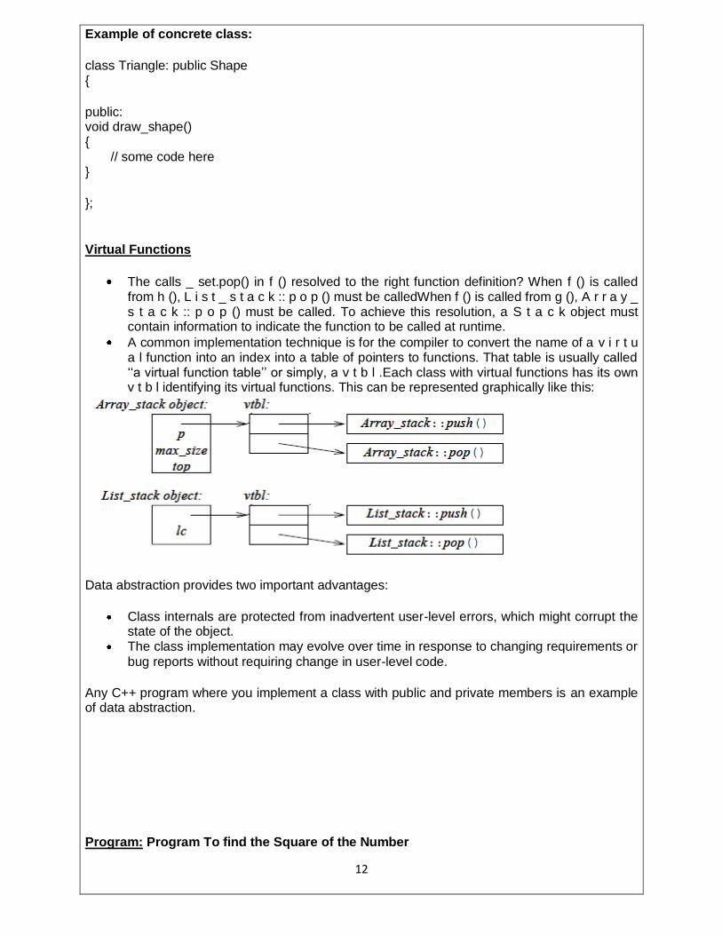
The calls _ set.pop() in f () resolved to the right function definition? When f () is called from h (), L i s t _ s t a c k :: p o p () must be calledWhen f () is called from g (), A r r a y _ s t a c k :: p o p () must be called. To achieve this resolution, a S t a c k object must contain information to indicate the function to be called at runtime.

A common implementation technique is for the compiler to convert the name of a v i r t u a l function into an index into a table of pointers to functions. That table is usually called „„a virtual function table‟‟ or simply, a v t b l .Each class with virtual functions has its own v t b l identifying its virtual functions. This can be represented graphically like this:

Data abstraction provides two important advantages:

Class internals are protected from inadvertent user-level errors, which might corrupt the state of the object.

The class implementation may evolve over time in response to changing requirements or

bug reports without requiring change in user-level code.

Any C++ program where you implement a class with public and private members is an example of data abstraction. Program: Program To find the Square of the Number

13

#include<iostream> #include<conio.h> classAdder{ public: // constructor Adder(int i =0) { total = i; } // interface to outside world voidaddNum(int number) { total += number; } // interface to outside world intgetTotal() { return total; }; private: // hidden data from outside world int total; }; int main() { Adder a; a.addNum(10); a.addNum(20); a.addNum(30); cout<<"Total "<<a.getTotal()<<endl; return0; } OUTPUT:

Total 60 Encapsulation:

Data Hiding is also known as Encapsulation. Encapsulation is the process of combining data and function into a single unit called class.

Data Hiding is the mechanism where the details of the class are hidden from the user.

The user can perform only a restricted set of operations in the hidden member of the class.

Encapsulation is a powerful feature that leads to information hiding,abstract data type and friend function.

They encapsulate all the essential properties of the object that are to be created.

Using the method of encapsulation the programmer cannot directly access the class.

14

Access Specifier:

There are three types of access specifier. They are Private :Within the block. Public:Whole over the class. Protected:Act as a public and then act as a private.

Within a class members can be declared as either public protected or private in order to explicitly enforce encapsulation. The elements placed after the public keyword is accessible to all the user of the class. The elements placed after the protected keyword is accessible only to the methods of the class. The elements placed after the private keyword are accessible only to the methods of the class. The data is hidden inside the class by declaring it as private inside the class. Thus private data cannot be directly accessed by the object. Syntax:

class class name { private: datatype data; public: Member functions; }; main() { classname objectname1,objectname2……………; }

Example: class Square {

private: int Num; public: void Get() { cout<<"Enter Number:"; cin>>Num;

} void Display()

{ cout<<"Square Is:"<<Num*Num; }

}; void main() {

Square Obj; Obj.Get(); Obj.Display(); getch()

} Output:

Enter Number: 10

Square is: 100

15

Features and Advantages of Data Encapsulation:

The advantage of data encapsulation comes when the implementation of the class

changes but the interface remains the same.

It is used to reduce the human errors. The data and function are bundled inside the class

that take total control of maintenance and thus human errors are reduced.

Makes maintenance of application easier.

Improves the understandability of the application.

Enhanced Security.

Classes:

A class is a userdefined type.

The aim of the C++ class concept is to provide the programmer with a tool for creating new types that can be used as conveniently as the builtin types.

The basic facilities for defining a class, creating objects of a class, and manipulating such objects are defined below:

Concepts and classes

Class members and Access control

Constructors

Static members

Default copy

Const member functions

This

Structure & Union

In-class function definition

member functions and helper functions

Overloaded operators

Use of concrete classes

Classes and object:

The mechanism that allows you to combine data and the function in a single unit is called a class.

Once a class is defined, you can declare variables of that type. A class variable is called object or instance.

In other words, a class would be the data type, and an object would be the variable.

Classes are generally declared using the keyword class, with the following format:

Syntax:

class class_name { private: members1; protected: members2; public: members3; };

16

Where class_name is a valid identifier for the class.

The body of the declaration can contain members, that can be either data or function declarations, The members of a class are classified into three categories:

1. Private 2. Public

3. protected.

Private, protected, and public are reserved words and are called member access specifiers. These specifiers modify the access rights that the members following them acquire.

private members of a class are accessible only from within other members of the same

class. You cannot access it outside of the class.

protected members are accessible from members of their same class and also from members of their derived classes. Finally, public members are accessible from

anywhere where the object is visible.

By default, all members of a class declared with the class keyword have private access for all its members. Therefore, any member that is declared before one other class specifier automatically has private access.

Here is a complete example :

class circle { private : double radius; public: void setRadius(double r) { radius = r; } double getArea() { return 3.14*radius*radius; } };

Object Declaration

Once a class is defined, you can declare objects of that type. The syntax for declaring a object is the same as that for declaring any other variable. The following statements declare two

objects of type circle:

circle c1, c2;

Accessing Class Members

Once an object of a class is declared, it can access the public members of the class.

c1.setRadius(2.5);

17

Defining Member function of class

Definingfunctions inside the class as shown in above example. Member functions defined inside a class this way are created as inline functions by default.

It is also possible to declare a function within a class but define it elsewhere.

Functions defined outside the class are not normally inline. When we define a function outside the class we cannot reference them (directly) outside of the class.

In order to reference these, we use the scope resolution operator, :: (double colon).

In this example, we are defining function setRadius outside the class:

void circle :: setRadius(double r) { radius = r; }

The following program demostrates the general feature of classes. Member functionssetRadius() and getArea() defined outside the class.

#include <iostream> #include<conio.h>

class circle //specify a class { private : double radius; //class data members public: void setRadius(double r); double getArea(); //member function to get data from user }; void circle :: setRadius(double r) { radius = r; } double circle :: getArea() { return 3.14*radius*radius; } int main() { circle c1; //define object of class circle c1.setRadius(2.5); //call member function to initialize cout<<c1.getArea(); return 0;

}

OUTPUT:

19.625

18

Struct and Class

• A struct is a class where members are public by default:

struct X { int m; // … };

• Means class X { public: int m; // … };

structs are primarily used for data structures where the members can take any value

Constructors& Destructor:

Constructor

It is a member function having same name as it‟s class and which is used to initialize the objects of that class type with a legal initial value. Constructor is automatically called when object is

created.

Types of Constructor

Default Constructor-: A constructor that accepts no parameters is known as default

constructor. If no constructor is defined then the compiler supplies a default constructor.It does not take any argument.

Syntax:

Class name()

{ constructor Definition }

Example:

circle :: circle() { radius = 0;

}

Parameterized Constructor -: A constructor that receives arguments/parameters, is called parameterized constructor. circle :: circle(double r) { radius = r;

}

19

Copy Constructor-: A constructor that initializes an object using values of another object passed to it as parameter, is called copy constructor. It creates the copy of the passed object. circle :: circle(circle &t) { radius = t.radius;

}

There can be multiple constructors of the same class, provided they have different signatures.

Destructor

A destructor is a member function having sane name as that of its class preceded by ~(tilde) sign and which is used to destroy the objects that have been created by a constructor. It gets invoked when an object‟s scope is over.

~circle() { }

Example : In the following program constructors, destructor and other member functions are defined inside class definitions. Since we are using multiple constructor in class so this example

also illustrates the concept of constructor overloading

#include<iostream> #include<conio.h> class circle //specify a class { private : double radius; //class data members

public: circle() //default constructor { radius = 0;

}

circle(double r) //parameterized constructor { radius = r;

}

circle(circle &t) //copy constructor { radius = t.radius; }

void setRadius(double r) //function to set data { radius = r; }

20

double getArea() { return 3.14*radius*radius; } ~circle() //destructor {}

}; int main() { circle c1; //defalut constructor invoked circle c2(2.5); //parmeterized constructor invoked circle c3(c2); //copy constructor invoked cout<<c1.getArea()<<endl; cout<<c2.getArea()<<endl; cout<<c3.getArea()<<endl; return 0;

}

Static Data & static member Functions:

A static data member is shared by all objects of the class in a program.

All static data is initialized to zero when the first object is created, if no other initialization

is present.

It can be initialized outside the class as done in the following example by redeclaring the

static variable, using the scope resolution operator :: to identify which class it belongs to.

Static member function

A static member function can be called even if no objects of the class exist and the static functions are accessed using only the class name and the scope resolution operator ::.

A static member function can only access static data member, other static member functions and any other functions from outside the class.

Static member functions have a class scope and they do not have access to the this pointer of the class. You could use a static member function to determine whether some

objects of the class have been created or not.

Syntax:

class Date { int d, m ,y; static Date default_date; public: Date(intdd=0;int mm=0;int yy=0); //… static void set_default(int , int, int); };

int main() { Date::set_default(10,20,30); // ok }

21

Program to find the count object:

#include<iostream.h> #include<conio.h> class stat { int code; static int count; public: stat() { code=++count; } void showcode() { cout<<"\n\tObject number is :"<<code; } static void showcount() { cout<<"\n\tCount Objects :"<<count; } }; int stat::count; void main() { clrscr(); stat obj1,obj2; obj1.showcount(); obj1.showcode(); obj2.showcount(); obj2.showcode(); getch(); } Output:

Count Objects: 2 Object Number is: 1 Count Objects: 2 Object Number is: 2

Const Member Functions:

Const is something that does not change.It is used to make the element constant.

Const member function implies that the member function will not change the state

of the object.

22

The data member of the class represents the “state” of the object. So, the const

member function grantees that it will not change the value in the data member till it

returns to the caller.

Const keyword can be used with

o Variables

o Pointers

o Function arguments and return types

o Class data members

o Class member functions

o Object

Constant variables:

const variables cannot be modified .It can be initialized during the declaration.

Syntax:

Constint i=10;

Pointer Variable:

Pointer is pointing to the const variable.

Syntax:

Constint *u;

Constant Function arguments and return types:

Return type and arguments are constant.They cannot be changed anywhere.

Syntax:

void f(constint i) { i++; } constint g() { return 1; }

Const objects:

An object declared as const cannot be modified and hence, can invoke only const member

functions as these functions ensure not to modify the object.

Syntax:

const class_name object_name;

23

Const class Data members:

This are data variables in class which are made const.They are not initialized during declaration.

There initialization occur in the constructor.

Example:

Class Test { constint i; Public: Test(int x) {

i=x; }}; int main() {

Test t(10); Test s(20);

}

Const class member functions:

A const member functions never modifies data members in an object.

Syntax:

return_typefunction_name() const;

Mutable keyword:

Mutable keyword is used with member variables of class which we want to change even if the

object is of consttype.mutable data members of const objects can be modified.

Syntax:

mutable int j;

Program

#include<iostream.h>

#include<conio.h>

class test { private: int data; public: test() { data=2; }

24

// this is an error by removing constructor.// void showdata()

{cout<<"data="<<data<<endl;}// it will give warning but access data.// void showdata()const; // it will work successfully.// void setdata()const { data=5;

} // it will generate an error.// void setdata() { data=5; }// it will give warning but modify the object. void test::showdata()const { cout<<" data = "<<data<<endl; } }; main( ) { clrscr(); const test obj; obj.showdata(); //obj.setdata(); getch(); return 0; } Output: data=2 Member Functions:

Function defined inside a class declaration is called as member function or method. Methods can be defined in two ways

Inside the class or outside the class using scope resolution operator (::)

When defined outside class declaration, function needs to be declared inside the class. Program to find Volume of the Box:

#include<iostream> #include<conio.h> classBox { public: double length;// Length of a box double breadth;// Breadth of a box double height;// Height of a box // Member functions declaration doublegetVolume(void); voidsetLength(doublelen); voidsetBreadth(doublebre); voidsetHeight(doublehei); }; // Member functions definitions doubleBox::getVolume(void) { return length * breadth * height; } voidBox::setLength(doublelen) { length =len; }

25

voidBox::setBreadth(doublebre) { breadth =bre; } voidBox::setHeight(doublehei) { height =hei; } // Main function for the program int main() { BoxBox1;// Declare Box1 of type Box BoxBox2;// Declare Box2 of type Box double volume =0.0;// Store the volume of a box here // box 1 specification Box1.setLength(6.0); Box1.setBreadth(7.0); Box1.setHeight(5.0); // box 2 specification Box2.setLength(12.0); Box2.setBreadth(13.0); Box2.setHeight(10.0); // volume of box 1 volume =Box1.getVolume(); cout<<"Volume of Box1 : "<< volume <<endl; // volume of box 2 volume =Box2.getVolume(); cout<<"Volume of Box2 : "<< volume <<endl; return0; } OUTPUT:

Volume of Box1 : 210

Volume of Box2 : 1560

Inline Member functions

C++ inline function is powerful concept that is commonly used with classes. If a function is inline, the compiler places a copy of the code of that function at each point where the function is

called at compile time.

Any change to an inline function could require all clients of the function to be recompiled because compiler would need to replace all the code once again otherwise it will continue with old functionality.

To inline a function, place the keyword inline before the function name and define the

function before any calls are made to the function. The compiler can ignore the inline qualifier in case defined function is more than a line.

A function definition in a class definition is an inline function definition, even without the use of the inline specifier.

26

#include<iostream.h>

#include<conio.h> inlineintMax(int x,int y) { return(x > y)? x : y; } // Main function for the program int main() { cout<<"Max (20,10): "<<Max(20,10)<<endl; cout<<"Max (0,200): "<<Max(0,200)<<endl; cout<<"Max (100,1010): "<<Max(100,1010)<<endl; return0; } OUTPUT:

Max (20,10): 20 Max (0,200): 200 Max (100,1010): 1010

Pointers:

A pointer is a variable that holds a memory address, usually the location of another variable in

memory.

Defining a Pointer Variable

int *iptr; iptr can hold the address of an int

Pointer Variables Assignment:

intnum = 25; int *iptr; iptr = &num;

Memory layout

To access num using iptr and indirection operator *

cout<<iptr; // prints 0x4a00 cout<< *itptr; // prints 25

Similary, following declaration shows: char *cptr; float *fptr; cptr is a pointer to character and fptr is a pointer to float value.

27

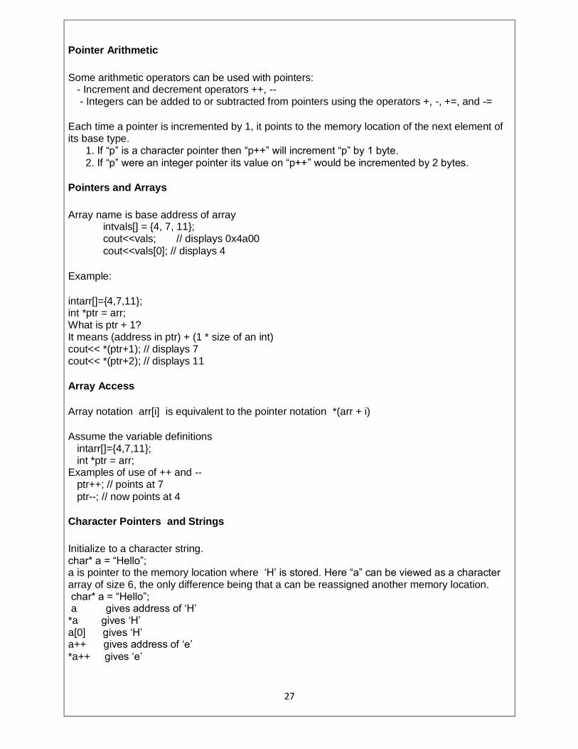
Pointer Arithmetic

Some arithmetic operators can be used with pointers: - Increment and decrement operators ++, -- - Integers can be added to or subtracted from pointers using the operators +, -, +=, and -=

Each time a pointer is incremented by 1, it points to the memory location of the next element of its base type. 1. If “p” is a character pointer then “p++” will increment “p” by 1 byte.

2. If “p” were an integer pointer its value on “p++” would be incremented by 2 bytes.

Pointers and Arrays

Array name is base address of array intvals[] = {4, 7, 11}; cout<<vals; // displays 0x4a00

cout<<vals[0]; // displays 4

Example:

intarr[]={4,7,11}; int *ptr = arr; What is ptr + 1? It means (address in ptr) + (1 * size of an int) cout<< *(ptr+1); // displays 7 cout<< *(ptr+2); // displays 11

Array Access

Array notation arr[i] is equivalent to the pointer notation *(arr + i)

Assume the variable definitions intarr[]={4,7,11}; int *ptr = arr; Examples of use of ++ and -- ptr++; // points at 7

ptr--; // now points at 4

Character Pointers and Strings

Initialize to a character string. char* a = “Hello”; a is pointer to the memory location where „H‟ is stored. Here “a” can be viewed as a character array of size 6, the only difference being that a can be reassigned another memory location. char* a = “Hello”; a gives address of „H‟ *a gives „H‟ a[0] gives „H‟ a++ gives address of „e‟

*a++ gives „e‟

28

Pointers as Function Parameters:

A pointer can be a parameter. It works like a reference parameter to allow change to argument from within function

Pointers as Function Parameters void swap(int *x, int *y) { int temp; temp = *x; *x = *y; *y = temp; } swap(&num1, &num2);

Pointers to Constants and Constant Pointers:

Pointer to a constant: cannot change the value that is pointed at

Constant pointer: address in pointer cannot change once pointer is initialized

Pointers to Structures:

We can create pointers to structure variables

struct Student {introllno; float fees;}; Student stu1; Student *stuPtr = &stu1; (*stuPtr).rollno= 104; -or-

Use the form ptr->member: stuPtr->rollno = 104;

Static allocation of memory

In the static memory allocation, the amount of memory to be allocated is predicted and preknown. This memory is allocated during the compilation itself. All the declared variables

declared normally, are allocated memory statically.

Dynamic allocation of memory

In the dynamic memory allocation, the amount of memory to be allocated is not known. This memory is allocated during run-time as and when required. The memory is dynamically

allocated using new operator.

Free store

Free store is a pool of unallocated heap memory given to a program that is used by the program for dynamic allocation during execution.

29

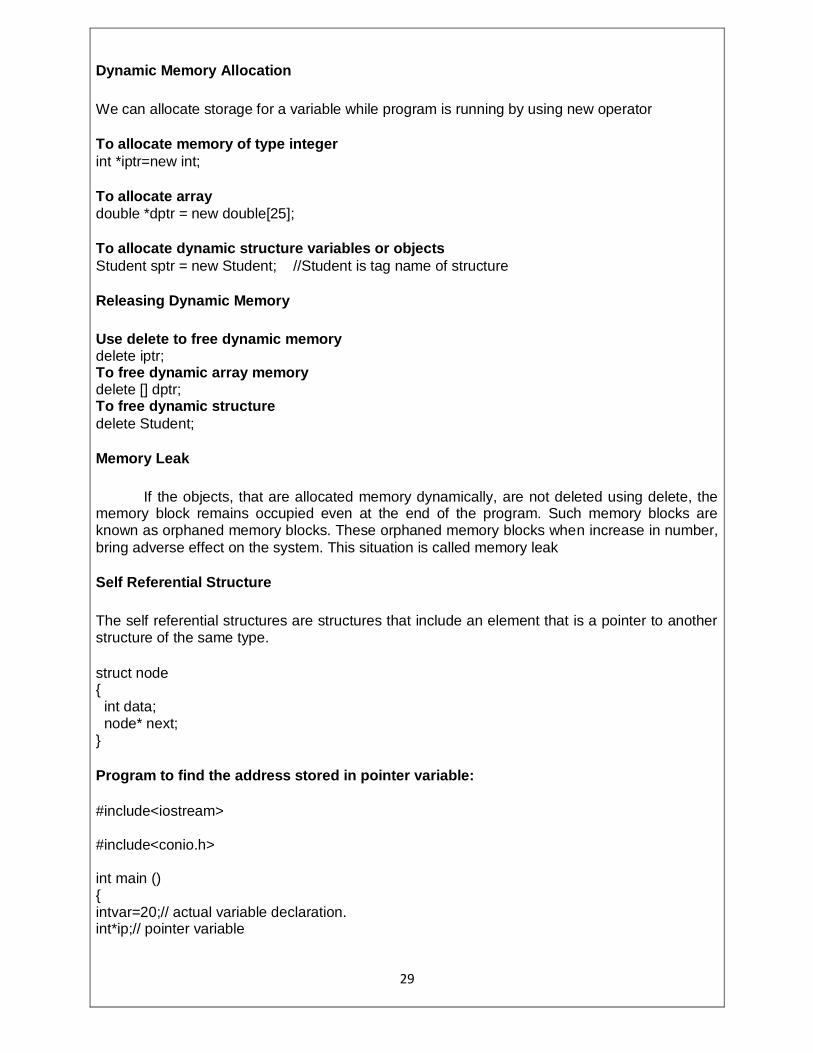
Dynamic Memory Allocation

We can allocate storage for a variable while program is running by using new operator

To allocate memory of type integer

int *iptr=new int;

To allocate array

double *dptr = new double[25];

To allocate dynamic structure variables or objects

Student sptr = new Student; //Student is tag name of structure

Releasing Dynamic Memory

Use delete to free dynamic memory delete iptr; To free dynamic array memory delete [] dptr; To free dynamic structure

delete Student;

Memory Leak

If the objects, that are allocated memory dynamically, are not deleted using delete, the memory block remains occupied even at the end of the program. Such memory blocks are known as orphaned memory blocks. These orphaned memory blocks when increase in number,

bring adverse effect on the system. This situation is called memory leak

Self Referential Structure

The self referential structures are structures that include an element that is a pointer to another structure of the same type.

struct node { int data; node* next; }

Program to find the address stored in pointer variable:

#include<iostream> #include<conio.h> int main () { intvar=20;// actual variable declaration. int*ip;// pointer variable

30

ip=&var;// store address of var in pointer variable cout<<"Value of var variable: "; cout<<var<<endl; // print the address stored in ip pointer variable cout<<"Address stored in ip variable: "; cout<<ip<<endl; // access the value at the address available in pointer cout<<"Value of *ip variable: "; cout<<*ip<<endl; return0; }

OUTPUT:

Value of var variable:20 Address stored inip variable:0xbfc601ac Value of *ip variable:20

References

References are often confused with pointers but three major differences between references and pointers are:

You cannot have NULL references. You must always be able to assume that a reference is connected to a legitimate piece of storage.

Once a reference is initialized to an object, it cannot be changed to refer to another object. Pointers can be pointed to another object at any time.

A reference must be initialized when it is created. Pointers can be initialized at any time

Creating References

Accessing the contents of the variable through either the original variable name or the

reference by the following syntax.

int i =17; creating the reference variable as

int& r = i; Read the & in these declarations as reference. Thus, read the first declaration as "r is an

integer reference initialized to i" and read the second declaration as "s is a double reference

initialized to d.".

Program: #include<iostream> #include<conio.h> int main () { // declare simple variables int i;

31

double d; // declare reference variables int& r = i; double& s = d; i =5; cout<<"Value of i : "<< i <<endl; cout<<"Value of i reference : "<< r <<endl; d =11.7; cout<<"Value of d : "<< d <<endl; cout<<"Value of d reference : "<< s <<endl; return0; }

OUTPUT:

Value of i :5 Value of i reference :5 Value of d :11.7 Value of d reference :11.7

Role of this pointer

Every object in C++ has access to its own address through an important pointer called this pointer. The this pointer is an implicit parameter to all member functions. Therefore, inside a member function, this may be used to refer to the invoking object.

Friend functions do not have a this pointer, because friends are not members of a class. Only member functions have a this pointer.

„this‟ pointer is a constant pointer that holds the memory address of the current object.

A static member function does not have a this pointer.

Program to find the contructor:

#include<iostream> #include<conio.h> classBox { public: // Constructor definition Box(double l=2.0,double b=2.0,double h=2.0) { cout<<"Constructor called."<<endl; length = l; breadth = b; height = h; } doubleVolume() { return length * breadth * height; } int compare(Box box) { returnthis->Volume()>box.Volume();

32

} private: double length;// Length of a box double breadth;// Breadth of a box double height;// Height of a box }; int main(void) { BoxBox1(3.3,1.2,1.5);// Declare box1 BoxBox2(8.5,6.0,2.0);// Declare box2 if(Box1.compare(Box2)) { cout<<"Box2 is smaller than Box1"<<endl; } else { cout<<"Box2 is equal to or larger than Box1"<<endl; } return0; }

OUTPUT:

Constructor called. Constructor called. Box2is equal to or larger than Box1

Storage Classes

A storage class defines the scope (visibility) and life-time of variables and/or functions within a C++ Program. These specifiers precede the type that they modify. There are following storage classes, which can be used in a C++ Program

auto register static extern

mutable

The auto Storage Class

The auto storage class is the default storage class for all local variables.

{ int mount; autoint month; }

The example above defines two variables with the same storage class, auto can only be used within functions, i.e., local variables.

33

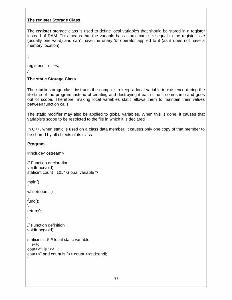
The register Storage Class

The register storage class is used to define local variables that should be stored in a register instead of RAM. This means that the variable has a maximum size equal to the register size (usually one word) and can't have the unary '&' operator applied to it (as it does not have a

memory location).

{

registerint miles; }

The static Storage Class

The static storage class instructs the compiler to keep a local variable in existence during the life-time of the program instead of creating and destroying it each time it comes into and goes out of scope. Therefore, making local variables static allows them to maintain their values between function calls.

The static modifier may also be applied to global variables. When this is done, it causes that

variable's scope to be restricted to the file in which it is declared

In C++, when static is used on a class data member, it causes only one copy of that member to

be shared by all objects of its class.

Program

#include<iostream> // Function declaration voidfunc(void); staticint count =10;/* Global variable */ main() { while(count--) { func(); } return0; } // Function definition voidfunc(void) { staticint i =5;// local static variable i++; cout<<"i is "<< i ; cout<<" and count is "<< count <<std::endl; }

34

OUTPUT

i is6and count is9 i is7and count is8 i is8and count is7 i is9and count is6 i is10and count is5 i is11and count is4 i is12and count is3 i is13and count is2 i is14and count is1 i is15and count is0

The extern Storage Class

The extern storage class is used to give a reference of a global variable that is visible to ALL the program files. When you use 'extern' the variable cannot be initialized as all it does is point the variable name at a storage location that has been previously defined.

When you have multiple files and you define a global variable or function, which will be used in other files also, then extern will be used in another file to give reference of defined variable or function. Just for understanding extern is used to declare a global variable or function in another file.

The extern modifier is most commonly used when there are two or more files sharing the same global variables or functions as explained below.

First File: main.cpp

#include<iostream> int count ; externvoidwrite_extern(); main() { count =5; write_extern(); }

Second File: support.cpp

#include<iostream> externint count; voidwrite_extern(void) { std::cout<<"Count is "<< count <<std::endl; }

Here, extern keyword is being used to declare count in another file. Now compile these two files as follows: $g++ main.cpp support.cpp -o write

This will produce write executable program, try to execute write and check the result as follows:

$./write

5

35

The mutable Storage Class

The mutable specifier applies only to class objects, It allows a member of an object to override

constness. That is, a mutable member can be modified by a const member function.

Function as arguments

Function

A function is a group of statements that together perform a task.

A function is a subprogram that acts on data and often returns a value.

A program written with numerous functions is easier to maintain, update and debug than one very long program.

By programming in a modular (functional) fashion, several programmers can work independently on separate functions which can be assembled at a later date to create

the entire project.

Defining a Function:

The general form of a C++ function definition is as follows:

return_typefunction_name( parameter list ) { body of the function }

A C++ function definition consists of a function header and a function body. Here are all the parts of a function:

Return Type: A function may return a value. The return_type is the data type of the

value the function returns. Some functions perform the desired operations without returning a value. In this case, the return_type is the keyword void.

Function Name: This is the actual name of the function. The function name and the parameter list together constitute the function signature.

Parameters: When a function is invoked, passing a value to the parameter. This value

is referred to as actual parameter or argument. Function Body: The function body contains a collection of statements that define what

the function does.

Function Declarations:

A function declaration tells the compiler about a function name and how to call the function.

The actual body of the function can be defined separately.

Syntax: return_typefunction_name( parameter list );

Eg:

int max(int num1,int num2);

36

Calling a Function:

While creating a C++ function, you give a definition of what the function has to do. To use a function, you will have to call or invoke that function.

When a program calls a function, program control is transferred to the called function. A called function performs defined task and when its return statement is executed or when its function-ending closing brace is reached, it returns program control back to the main

program.

#include<iostream> #include<conio.h> // function declaration int max(int num1,int num2); int main () { // local variable declaration: int a =100; int b =200; int ret; // calling a function to get max value. ret = max(a, b); cout<<"Max value is : "<< ret <<endl; return0; } // function returning the max between two numbers int max(int num1,int num2) { // local variable declaration int result; if(num1 > num2) result = num1; else result = num2; return result; }

I kept max() function along with main() function and compiled the source code. While running final executable, it would produce the following result:

Max value is : 200

37

Function Arguments:

If a function is to use arguments, it must declare variables that accept the values of the arguments. These variables are called the formal parameters of the function.

The formal parameters behave like other local variables inside the function and are created upon entry into the function and destroyed upon exit.

While calling a function, there are three ways that arguments can be passed to a

function:

Call Type Description

Call by value

This method copies the actual value of an argument into the formal

parameter of the function. In this case, changes made to the

parameter inside the function have no effect on the argument.

Call by pointer

This method copies the address of an argument into the formal

parameter. Inside the function, the address is used to access the

actual argument used in the call. This means that changes made

to the parameter affect the argument.

Call by reference

This method copies the reference of an argument into the formal

parameter. Inside the function, the reference is used to access the

actual argument used in the call. This means that changes made

to the parameter affect the argument.

Call By Value: In call by value method, the called function creates its own copies of original values sent to it. Any changes, that are made, occur on the function‟s copy of values and are not reflected back to the calling function. Syntax:

// function definition to swap the values. void swap(int x,int y) { int temp; temp = x;/* save the value of x */ x = y;/* put y into x */ y = temp;/* put x into y */ return; } Program to find swapping of the number by call by value:

#include<iostream> #include<conio.h> // function declaration void swap(int x,int y);

38

int main () { // local variable declaration: int a =100; int b =200; cout<<"Before swap, value of a :"<< a <<endl; cout<<"Before swap, value of b :"<< b <<endl; // calling a function to swap the values. swap(a, b); cout<<"After swap, value of a :"<< a <<endl; cout<<"After swap, value of b :"<< b <<endl; return0; }

Output:

Before swap, value of a :100 Before swap, value of b :200 After swap, value of a :100 After swap, value of b :200

Call by pointer

The call by pointer method of passing arguments to a function copies the address of an

argument into the formal parameter. Inside the function, the address is used to access the actual argument used in the call. This means that changes made to the parameter affect the passed argument.

syntax:

// function definition to swap the values. void swap(int*x,int*y) { int temp; temp =*x;/* save the value at address x */ *x =*y;/* put y into x */ *y = temp;/* put x into y */ return; }

Program to find swapping of the number by call by pointer:

#include<iostream> #include<conio.h> // function declaration void swap(int*x,int*y); int main () { // local variable declaration: int a =100; int b =200; cout<<"Before swap, value of a :"<< a <<endl;

39

cout<<"Before swap, value of b :"<< b <<endl; /* calling a function to swap the values. * &a indicates pointer to a ie. address of variable a and * &b indicates pointer to b ie. address of variable b. */ swap(&a,&b); cout<<"After swap, value of a :"<< a <<endl; cout<<"After swap, value of b :"<< b <<endl; return0; }

Output:

Before swap, value of a :100 Before swap, value of b :200 After swap, value of a :200 After swap, value of b :100

Call by Reference:

The call by reference method of passing arguments to a function copies the reference

of an argument into the formal parameter. Inside the function, the reference is used to access the actual argument used in the call. This means that changes made to the parameter affect the

passed argument.

Syntax:

// function definition to swap the values. void swap(int&x,int&y) { int temp; temp = x;/* save the value at address x */ x = y;/* put y into x */ y = temp;/* put x into y */ return; } Program to find swapping of the number by call by Reference:

#include<iostream> #include<conio.h> // function declaration void swap(int&x,int&y); int main () { // local variable declaration: int a =100; int b =200; cout<<"Before swap, value of a :"<< a <<endl; cout<<"Before swap, value of b :"<< b <<endl; /* calling a function to swap the values using variable reference.*/ swap(a, b); cout<<"After swap, value of a :"<< a <<endl; cout<<"After swap, value of b :"<< b <<endl; return0; }

40

Output:

Before swap, value of a :100

Before swap, value of b :200

After swap, value of a :200

After swap, value of b :100

CS6301 – PROGRAMMING & DATA STRUCTURES II

UNIT II

OBJECT ORIENTED PROGRAMMING CONCEPTS

String Handling – Copy Constructor - Polymorphism – compile time and run time polymorphisms –function overloading – operators overloading – dynamic memory allocation - Nested classes -Inheritance – virtual functions.

String Handling

String is a one-dimensional array of characters which is terminated by a null character

'\0'. Thus a null-terminated string contains the characters that comprise the string followed by a null.

Useful C functions for string manipulation in <cstring>header (C++ name for string.h)

The following declaration and initialization create a string consisting of the word "Hello". To hold the null character at the end of the array, the size of the character array containing the

string is one more than the number of characters in the word "Hello."

char greeting[6] = {'H', 'e', 'l', 'l', 'o', '\0'};

Following the rule of array initialization, then write the above statement as follows:

char greeting[] = "Hello";

Following is the memory presentation of above defined string in C/C++:

Actually, you do not place the null character at the end of a string constant. The C++ compiler automatically places the '\0' at the end of the string when it initializes the array.

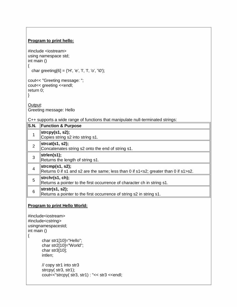
Program to print hello:

#include <iostream> using namespace std; int main () { char greeting[6] = {'H', 'e', 'l', 'l', 'o', '\0'}; cout<< "Greeting message: "; cout<< greeting <<endl; return 0; } Output: Greeting message: Hello C++ supports a wide range of functions that manipulate null-terminated strings:

S.N. Function & Purpose

1 strcpy(s1, s2); Copies string s2 into string s1.

2 strcat(s1, s2); Concatenates string s2 onto the end of string s1.

3 strlen(s1); Returns the length of string s1.

4 strcmp(s1, s2); Returns 0 if s1 and s2 are the same; less than 0 if s1<s2; greater than 0 if s1>s2.

5 strchr(s1, ch);

Returns a pointer to the first occurrence of character ch in string s1.

6 strstr(s1, s2);

Returns a pointer to the first occurrence of string s2 in string s1.

Program to print Hello World:

#include<iostream> #include<cstring> usingnamespacestd; int main () {

char str1[10]="Hello"; char str2[10]="World"; char str3[10]; intlen; // copy str1 into str3 strcpy( str3, str1); cout<<"strcpy( str3, str1) : "<< str3 <<endl;

// concatenates str1 and str2 strcat( str1, str2); cout<<"strcat( str1, str2): "<< str1 <<endl; // total lenghth of str1 after concatenation len=strlen(str1); cout<<"strlen(str1) : "<<len<<endl; return0;

}

OUTPUT:

strcpy( str3, str1):Hello strcat( str1, str2):HelloWorld strlen(str1):10

String Class in C++:

The standard C++ library provides a string class type that supports all the operations

mentioned above, additionally much more functionality.

#include<iostream> #include<string> int main () {

string str1 ="Hello"; string str2 ="World"; string str3; intlen; // copy str1 into str3 str3 = str1; cout<<"str3 : "<< str3 <<endl; // concatenates str1 and str2 str3 = str1 + str2; cout<<"str1 + str2 : "<< str3 <<endl; // total lenghth of str3 after concatenation len= str3.size(); cout<<"str3.size() : "<<len<<endl; return0;

}

Output:

str3 :Hello str1 +str2 :HelloWorld str3.size():10

Copy Constructor:

The copy constructor is a constructor which creates an object by initializing it with an object of

the same class, which has been created previously. The copy constructor is used to:

Initialize one object from another of the same type. Copy an object to pass it as an argument to a function. Copy an object to return it from a function.

If a copy constructor is not defined in a class, the compiler itself defines one.If the class has pointer variables and has some dynamic memory allocations, then it is a must to have a copy

constructor.

Syntax:

classname(constclassname&obj){ // body of constructor } Program for copy constructor to print the details of memory: #include<iostream> usingnamespacestd; classLine { public: intgetLength(void); Line(intlen);// simple constructor Line(constLine&obj);// copy constructor ~Line();// destructor private: int*ptr; }; // Member functions definitions including constructor Line::Line(intlen) { cout<<"Normal constructor allocating ptr"<<endl; // allocate memory for the pointer; ptr=newint; *ptr=len; } Line::Line(constLine&obj) { cout<<"Copy constructor allocating ptr."<<endl; ptr=newint; *ptr=*obj.ptr;// copy the value }

Line::~Line(void) { cout<<"Freeing memory!"<<endl; deleteptr; } intLine::getLength(void) { return*ptr; } void display(Lineobj) { cout<<"Length of line : "<<obj.getLength()<<endl; } // Main function for the program int main() { Lineline(10); display(line); return0; }

OUTPUT:

Normal constructor allocating ptr Copy constructor allocating ptr. Length of line : 10 Freeing memory! Freeing memory!

Polymorphism

Polymorphism is the ability to use an operator or function in different ways.

Polymorphism gives different meanings or functions to the operators or functions.

Poly, referring too many, signifies the many uses of these operators and functions.

A single function usage or an operator functioning in many ways can be called polymorphism.

Polymorphism refers to codes, operations or objects that behave differently in different contexts.

"Overriding is the example of run-time polymorphism" "Overloading is the example of compile-time polymorphism."

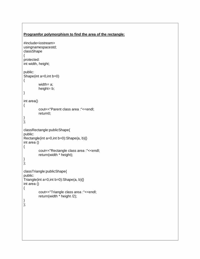
Programfor polymorphism to find the area of the rectangle:

#include<iostream> usingnamespacestd; classShape { protected: int width, height; public: Shape(int a=0,int b=0) { width= a; height= b; } int area() { cout<<"Parent class area :"<<endl; return0; } }; classRectangle:publicShape{ public: Rectangle(int a=0,int b=0):Shape(a, b){} int area () { cout<<"Rectangle class area :"<<endl; return(width * height); } }; classTriangle:publicShape{ public: Triangle(int a=0,int b=0):Shape(a, b){} int area () { cout<<"Triangle class area :"<<endl; return(width * height /2); } };

// Main function for the program int main() {

Shape*shape; Rectanglerec(10,7); Triangle tri(10,5); // store the address of Rectangle shape=&rec; // call rectangle area. shape->area(); // store the address of Triangle shape=&tri; // call triangle area. shape->area(); return0;

}

OUTPUT:

Parentclass area Parentclass area

Types of Polymorphism: C++ provides two different types of polymorphism.

run-time compile-time

run-time:

The appropriate member function could be selected while the programming is running. This is known as run-time polymorphism. The run-time polymorphism is implemented with inheritance and virtual functions.

Virtual functions

Virtual functions

A function qualified by the virtual keyword. When a virtual function is called via a pointer, the class of the object pointed to determines which function definition will be used.

Virtual functions implement polymorphism, whereby objects belonging to different classes can respond to the same message in different ways.

A virtual function is a function in a base class that is declared using the keyword virtual.

Defining in a base class a virtual function, with another version in a derived class,signals to the compiler that we don't want static linkage for this function.

What we do want is the selection of the function to be called at any given point in the program to be based on the kind of object for which it is called. This sort of operation is referred to as dynamic linkage, or late binding.

Program for Virtual Fuction to print base class

#include<iostream.h> #include<conio.h> class base { public: virtual void show() { cout<<"\n Base class show:"; } void display() { cout<<"\n Base class display:" ; } }; classdrive:public base { public: void display() { cout<<"\n Drive class display:"; } void show() { cout<<"\n Drive class show:"; } }; void main() { clrscr(); base obj1; base *p; cout<<"\n\t P points to base:\n" ; p=&obj1; p->display(); p->show(); cout<<"\n\n\t P points to drive:\n"; drive obj2; p=&obj2; p->display(); p->show(); getch(); }

Output:

P points to Base Base class display Base class show P points to Drive Base class Display Drive class Show compile-time:

The compiler is able to select the appropriate function for a particular call at compile-time itself. This is known as compile-time polymorphism. The compile-time polymorphism is implemented with templates.

Function name overloading Operator overloading

Function Overloading Using a single function name to perform different types of tasks is known as function

overloading.

Using the concept of function overloading, design a family of functions with one function name but with different argument lists.

The function would perform different operations depending on the argument list in the

function call.

The correct function to be invoked is determined by checking the number and type of the

arguments but not on the function type.

Syntax:

int test() { } int test(int a){ } int test(double a){ } int test(int a, double b){ }

Program for function overloading to create object and to delete object:

#include<iostream.h> #include<conio.h> classfover { public: inta,b,c; floatx,y,z;

fover() { cout<<" object is created:"; } void add(inta,int b) { c=a+b; cout<<"\n the addtion values:" <<c; } void add(float x,float y) { z=x+y; cout<<"\n the addtion values"<<z; } ~fover() { cout<<"\n the object is deleted"; } }; void main() {

inta,b; floatx,y; clrscr(); fover f; cout<<"\n enter the integer value"; cin>>a>>b; f.add(a,b); cout<<"\n enter the float values:"; cin>>x>>y; f.add(x,y); getch();

} OUTPUT:

object is created: enter the integer value3 4 theaddtion values:7 enter the float values:2.4 2.6 theaddtion values 5 the object is deleted

Operator Overloading

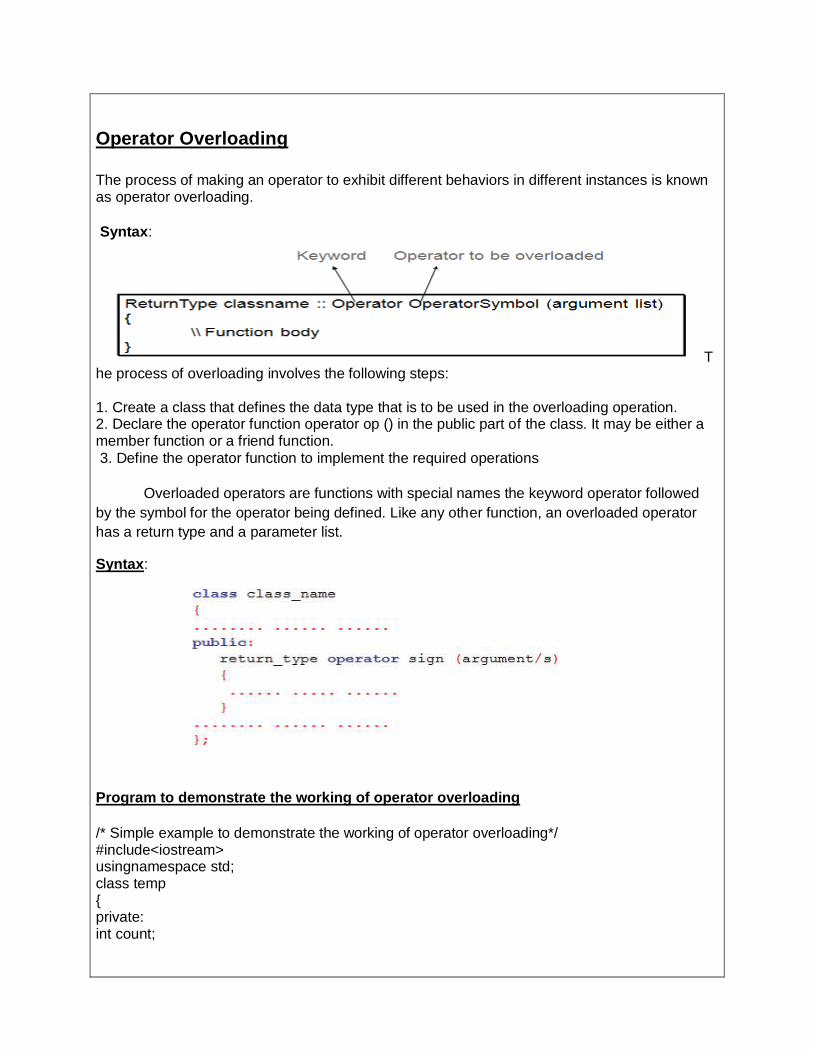
The process of making an operator to exhibit different behaviors in different instances is known as operator overloading.

Syntax:

The process of overloading involves the following steps: 1. Create a class that defines the data type that is to be used in the overloading operation. 2. Declare the operator function operator op () in the public part of the class. It may be either a member function or a friend function.

3. Define the operator function to implement the required operations

Overloaded operators are functions with special names the keyword operator followed

by the symbol for the operator being defined. Like any other function, an overloaded operator

has a return type and a parameter list.

Syntax:

Program to demonstrate the working of operator overloading

/* Simple example to demonstrate the working of operator overloading*/ #include<iostream> usingnamespace std; class temp { private: int count;

public: temp():count(5){} voidoperator++(){ count=count+1; } voidDisplay(){cout<<"Count: "<<count;} }; int main() {

temp t; ++t;/* operator function void operator ++() is called */ t.Display(); return0;

}

Output:Count: 6

Program2: Implementation of complex number class with operatoroverloading and type conversions #include<iostream.h> #include<conio.h> #include<math.h> class complex {float real,img,temp; public: complex() { real=img=0; } complex(int a) { real=a; img=0; } complex(double a1) { real=a1; img=0.0; } voidoutdata() {

if(img>=0.0) { cout<<real<<"+"<<img<<"i"; }

else {cout<<real<<img<<"i"; }} complex operator+(complex c) {

complex temp; temp.real=real+c.real; temp.img=img+c.img; return(temp);

}

complex operator-(complex c) {

complex temp1; temp1.real=real-c.real; temp1.img=img-c.img; return(temp1); }

complex operator*(complex c) {

complex temp2; temp2.real=real*c.real-img*c.img; temp2.img=real*c.img+img*c.real; return(temp2);

} complex operator/(complex c) {complex temp3; temp3.real=(((real*c.real)+(img*c.img))/((c.real*c.real)+(c.img*c.img))); temp3.img=(((img*c.real)-(real*c.img))/((c.real*c.real)+(c.img*c.img))); return(temp3); } operator double() {

double magnitude; magnitude=sqrt(pow(real,2)+pow(img,2)); return magnitude;

}}; void main() {

complex c1,c2,c3,c4,c5,c6; int real; double real1; cout<<"Enter the real number"; cin>>real; c1=real; cout<<"Integer to complex conversion"<<endl; cout<<"Enter the real number"; cin>>real1; c2=real1; cout<<"Double to complex conversion"<<endl; c3=c1+c2; c4=c1-c2; c5=c1*c2; c6=c1/c2; cout<<"\n\n"; cout<<"addtion result is:"; c3.outdata(); cout<<"\n\n"; cout<<"subraction result is:"; c4.outdata(); cout<<"\n\n"; cout<<"multiplication result is:"; c5.outdata(); cout<<"\n\n"; cout<<"division result is:"; c6.outdata(); cout<<"Conversion from complex to double"<<endl; double mag=c3; cout<<"Magnitude of a complex number"<<mag;

} Output

Enter the real number:2 Integer to complex conversion Enter the real number:2.0 Double to complex conversion addtion result is:4+0i subraction result is:0+0i multiplication result is:4+0i division result is:1+0i Conversion from complex to double Magnitude of a complex number:4

Friend function and Friend class:

A C++ friend functions are special functions which can access the private members of a

class.For instance: when it is not possible to implement some function, without making private

members accessible in them. This situation arises mostly in case of operator overloading.

Program to find friend function to print the mean value:

#include<iostream.h> #include<conio.h> class base { int val1,val2; public: void get() { cout<<"Enter two values:"; cin>>val1>>val2; } friend float mean(base ob); }; float mean(base ob) { return float(ob.val1+ob.val2)/2; } void main() { clrscr(); baseobj; obj.get(); cout<<"\n Mean value is : "<<mean(obj); getch(); }

Output:

Enter two values: 10, 20 Mean Value is: 15

Friend functions have the following properties:

Friend of the class can be member of some other class. Friend of one class can be friend of another class or all the classes in one program, such

a friend is known as GLOBAL FRIEND. Friend can access the private or protected members of the class in which they are

declared to be friend, but they can use the members for a specific object. Friends are non-members hence do not get “this” pointer. Friends, can be friend of more than one class, hence they can be used for message

passing between the classes. Friend can be declared anywhere (in public, protected or private section) in the class.

Friend Class:

A class can also be declared to be the friend of some other class. When we create a

friend class then all the member functions of the friend class also become the friend of

the other class. This requires the condition that the friend becoming class must be first

declared or defined (forward declaration).

They are used when two or more classes need to work together and need access of each other’s data members without making them accessible by other classes.

Program for friend class:

#include <iostream> #include<conio.h> class circle() {

Float r; Public: void get() { Cin>>r; Friend class Area;

}; class Area() {

Float getArea(Circle a) { Return 3.14*a.r*a.r; }

};

void main() {

Circle c; Area a; c.get(); float area=a.getArea(c); cout<<”area of circle:”<<area;

}

Dynamic Memory Allocation

Memory in your C++ program is divided into two parts:

The stack: All variables declared inside the function will take up memory from the stack. The heap: This is unused memory of the program and can be used to allocate the

memory dynamically when program runs.

Many times, you are not aware in advance how much memory you will need to store particular information in a defined variable and the size of required memory can be determined at run time.

You can allocate memory at run time within the heap for the variable of a given type using a special operator in C++ which returns the address of the space allocated. This operator is called new operator.

If you are not in need of dynamically allocated memory anymore, you can use delete operator,

which de-allocates memory previously allocated by new operator.

The new and delete operators:

There is following generic syntax to use new operator to allocate memory dynamically for any

data-type.

new data-type;

Here, data-type could be any built-in data type including an array or any user defined data

types include class or structure. Let us start with built-in data types.

For example we can define a pointer to type double and then request that the memory be allocated at execution time. We can do this using the new operator with the following

statements:

double*pvalue= NULL;// Pointer initialized with null pvalue=newdouble;// Request memory for the variable

The memory may not have been allocated successfully, if the free store had been used up. So it is good practice to check if new operator is returning NULL pointer and take appropriate action

as below:

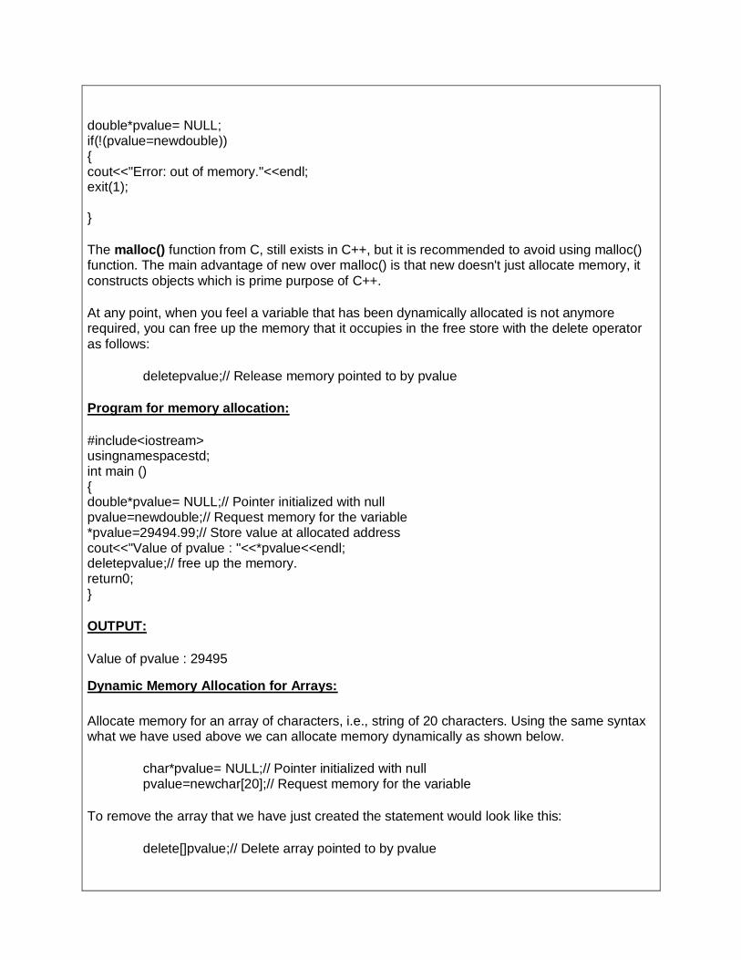
double*pvalue= NULL; if(!(pvalue=newdouble)) { cout<<"Error: out of memory."<<endl; exit(1); }

The malloc() function from C, still exists in C++, but it is recommended to avoid using malloc() function. The main advantage of new over malloc() is that new doesn't just allocate memory, it

constructs objects which is prime purpose of C++.

At any point, when you feel a variable that has been dynamically allocated is not anymore required, you can free up the memory that it occupies in the free store with the delete operator

as follows:

deletepvalue;// Release memory pointed to by pvalue

Program for memory allocation:

#include<iostream> usingnamespacestd; int main () { double*pvalue= NULL;// Pointer initialized with null pvalue=newdouble;// Request memory for the variable *pvalue=29494.99;// Store value at allocated address cout<<"Value of pvalue : "<<*pvalue<<endl; deletepvalue;// free up the memory. return0; }

OUTPUT:

Value of pvalue : 29495

Dynamic Memory Allocation for Arrays:

Allocate memory for an array of characters, i.e., string of 20 characters. Using the same syntax what we have used above we can allocate memory dynamically as shown below.

char*pvalue= NULL;// Pointer initialized with null pvalue=newchar[20];// Request memory for the variable

To remove the array that we have just created the statement would look like this:

delete[]pvalue;// Delete array pointed to by pvalue

Following the similar generic syntax of new operator, you can allocate for a multi-dimensional

array as follows:

double**pvalue= NULL;// Pointer initialized with null pvalue=newdouble[3][4];// Allocate memory for a 3x4 array

However, the syntax to release the memory for multi-dimensional array will still remain same as above:

delete[]pvalue;// Delete array pointed to by pvalue

Dynamic Memory Allocation for Objects:

Objects are no different from simple data types.Program for array of objects.

#include<iostream> usingnamespace std; classBox { public: Box(){ cout<<"Constructor called!"<<endl; } ~Box(){ cout<<"Destructor called!"<<endl; } }; int main() { Box*myBoxArray=newBox[4]; delete[]myBoxArray;// Delete array return0; } If you were to allocate an array of four Box objects, the Simple constructor would be called four times and similarly while deleting these objects, destructor will also be called same number of times.

Output:

Constructor called! Constructor called! Constructor called! Constructor called! Destructor called! Destructor called! Destructor called! Destructor called!

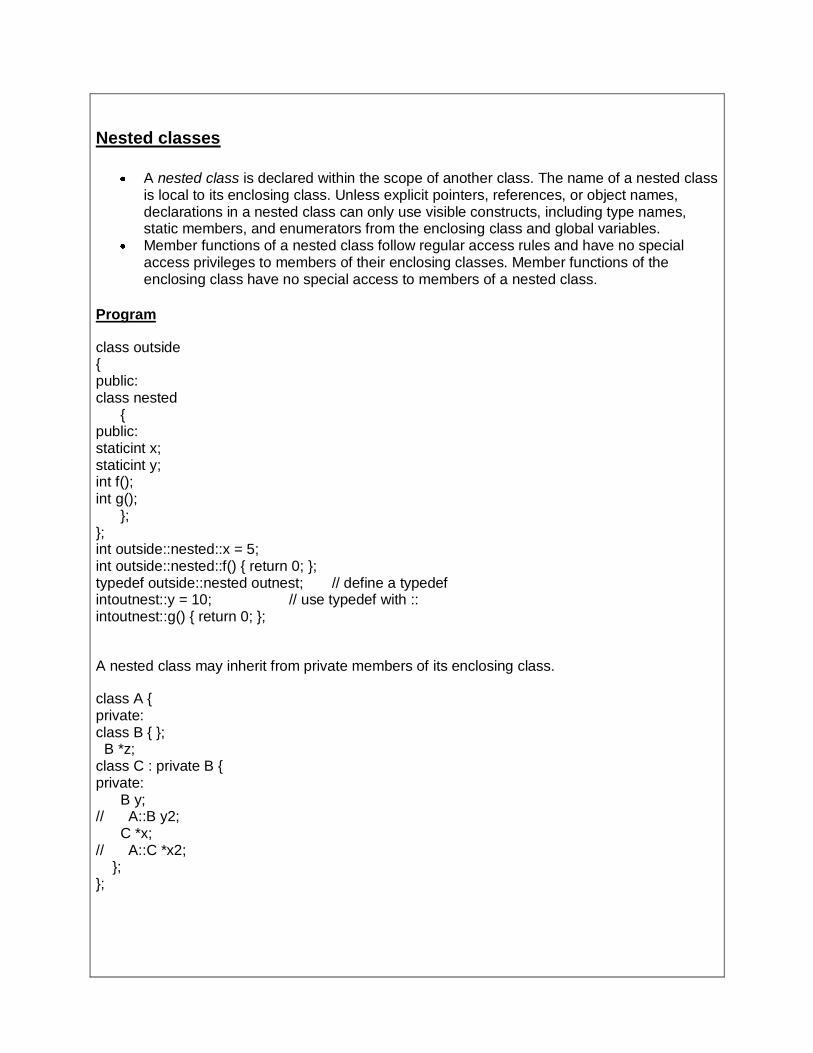
Nested classes

A nested class is declared within the scope of another class. The name of a nested class is local to its enclosing class. Unless explicit pointers, references, or object names, declarations in a nested class can only use visible constructs, including type names, static members, and enumerators from the enclosing class and global variables.

Member functions of a nested class follow regular access rules and have no special access privileges to members of their enclosing classes. Member functions of the enclosing class have no special access to members of a nested class.

Program

class outside { public: class nested { public: staticint x; staticint y; int f(); int g(); }; }; int outside::nested::x = 5; int outside::nested::f() { return 0; }; typedef outside::nested outnest; // define a typedef intoutnest::y = 10; // use typedef with :: intoutnest::g() { return 0; };

A nested class may inherit from private members of its enclosing class.

class A { private: class B { }; B *z; class C : private B { private: B y; // A::B y2; C *x; // A::C *x2; }; };

Inheritance

The mechanism that allows us to extend the definition of a class without making any physical changes to the existing class is inheritance.

Inheritance lets you create new classes from existing class. Any new class that you create from an existing class is called derived class; existing class is called base class.

The inheritance relationship enables a derived class to inherit features from its base class. Furthermore, the derived class can add new features of its own. Therefore, rather than create completely new classes from scratch, you can take advantage of inheritance

and reduce software complexity.

Forms of Inheritance

Single Inheritance: It is the inheritance hierarchy wherein one derived class inherits from one base class. Multiple Inheritance: It is the inheritance hierarchy wherein one derived class inherits from

multiple base class(es) Hierarchical Inheritance: It is the inheritance hierarchy wherein multiple subclasses inherit

from one base class. Multilevel Inheritance: It is the inheritance hierarchy wherein subclass acts as a base class for

other classes.

Syntax:

class derived-class: access baseA, access baseB....

Hybrid Inheritance: The inheritance hierarchy that reflects any legal combination of other four

types of inheritance.

In order to derive a class from another, we use a colon (:) in the declaration of the derived class

using the following format :

classderived_class: memberAccessSpecifierbase_class { ... };

Where derived_class is the name of the derived class and base_class is the name of the class on which it is based. The member Access Specifier may be public, protected or private. This access specifier describes the access level for the members that are inherited from the base

class.

Member Access Specifier

How Members of the Base Class Appear in the Derived Class

Private Private members of the base class are inaccessible to the derived class.

Protected members of the base class become private members of the derived class.

Public members of the base class become private members of the derived class.

Protected Private members of the base class are inaccessible to the derived class.

Protected members of the base class become protected members of the derived class.

Public members of the base class become protected members of the derived class.

Public Private members of the base class are inaccessible to the derived class.

Protected members of the base class become protected members of the derived class.

Public members of the base class become public members of the derived class.

Program for Single Inheritance to print HRA,DA and Net Pay

#include<iostream.h> #include<conio.h> classemp { public: inteno; char name[20],des[20]; void get() { cout<<"Enter the employee number:"; cin>>eno; cout<<"Enter the employee name:";

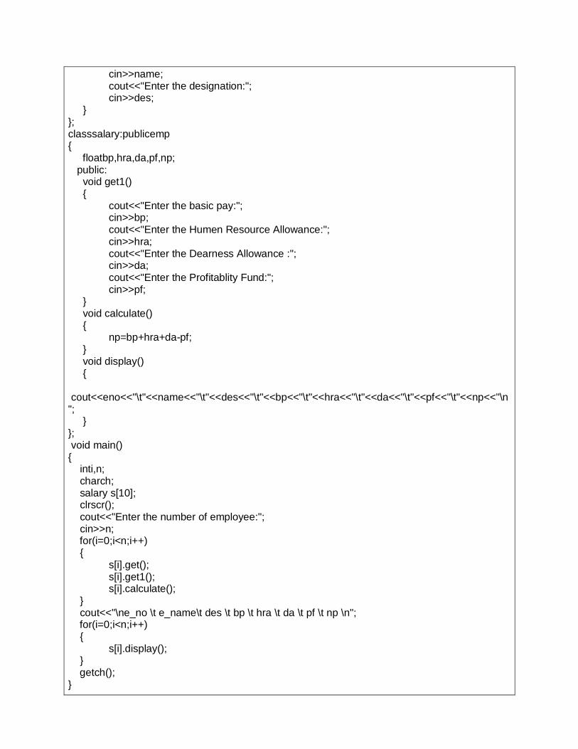
cin>>name; cout<<"Enter the designation:"; cin>>des; } }; classsalary:publicemp { floatbp,hra,da,pf,np; public: void get1() { cout<<"Enter the basic pay:"; cin>>bp; cout<<"Enter the Humen Resource Allowance:"; cin>>hra; cout<<"Enter the Dearness Allowance :"; cin>>da; cout<<"Enter the Profitablity Fund:"; cin>>pf; } void calculate() { np=bp+hra+da-pf; } void display() { cout<<eno<<"\t"<<name<<"\t"<<des<<"\t"<<bp<<"\t"<<hra<<"\t"<<da<<"\t"<<pf<<"\t"<<np<<"\n"; } }; void main() { inti,n; charch; salary s[10]; clrscr(); cout<<"Enter the number of employee:"; cin>>n; for(i=0;i<n;i++) { s[i].get(); s[i].get1(); s[i].calculate(); } cout<<"\ne_no \t e_name\t des \t bp \t hra \t da \t pf \t np \n"; for(i=0;i<n;i++) { s[i].display(); } getch(); }

Output:

Enter the Number of employee:1 Enter the employee No: 150 Enter the employee Name: ram Enter the designation: Manager Enter the basic pay: 5000 Enter the HR allowance: 1000 Enter the Dearness allowance: 500 Enter the profitability Fund: 300 E.No E.name des BP HRA DA PF NP 150 ram Manager 5000 1000 500 300 6200

Program for Multiple Inheritance to print student details:

#include<iostream.h> #include<conio.h> class student { protected: int rno,m1,m2; public: void get() { cout<<"Enter the Roll no :"; cin>>rno; cout<<"Enter the two marks :"; cin>>m1>>m2; } }; class sports { protected: intsm; // sm = Sports mark public: voidgetsm() { cout<<"\nEnter the sports mark :"; cin>>sm; } };

classstatement:publicstudent,public sports { inttot,avg; public: void display() { tot=(m1+m2+sm); avg=tot/3; cout<<"\n\n\tRoll No : "<<rno<<"\n\tTotal : "<<tot; cout<<"\n\tAverage : "<<avg; } }; void main() { clrscr(); statementobj; obj.get(); obj.getsm(); obj.display(); getch(); }

Output:

Enter the Roll no: 100 Enter two marks 90 80 Enter the Sports Mark: 90 Roll No: 100 Total : 260 Average: 86.66

Virtual Functions

A function qualified by the virtual keyword. When a virtual function is called via a pointer, the class of the object pointed to determines which function definition will be used. Virtual functions implement polymorphism, whereby objects belonging to different classes can respond to the same message in different ways.

A virtual function is a function in a base class that is declared using the keyword virtual.

Defining in a base class a virtual function, with another version in a derived class, signals to the compiler that we don't want static linkage for this function.

What we do want is the selection of the function to be called at any given point in the program to be based on the kind of object for which it is called. This sort of operation is referred to as dynamic linkage, or late binding.

Program for Virtual Function to base and derived class:

#include<iostream.h> #include<conio.h> class base { public: virtual void show() { cout<<"\n Base class show:"; } void display() { cout<<"\n Base class display:" ; } }; classdrive:public base { public: void display() { cout<<"\n Drive class display:"; } void show() { cout<<"\n Drive class show:"; } }; void main() { clrscr(); base obj1; base *p; cout<<"\n\t P points to base:\n" ; p=&obj1; p->display(); p->show(); cout<<"\n\n\t P points to drive:\n"; drive obj2; p=&obj2; p->display(); p->show();

getch(); }

Output:

P points to Base Base class display Base class show P points to Drive Base class Display Drive class Show

UNIT III

C++ Programming Advanced Features

Abstract Class

An interface describes the behavior or capabilities of a C++ class without committing to a particular implementation of that class.

The C++ interfaces are implemented using abstract classes and these abstract classes should not be confused with data abstraction which is a concept of keeping implementation details separate from associated data. A class is made abstract by declaring at least one of its functions as pure virtual function. A pure virtual function is specified by placing "= 0" in its declaration as follows:

class Box

{

public:

// pure virtual function

virtual double getVolume() = 0;

private:

double length; // Length of a box

double breadth; // Breadth of a box

double height; // Height of a box

};

The purpose of an abstract class (often referred to as an ABC) is to provide an appropriate base class from which other classes can inherit. Abstract classes cannot be used to instantiate objects and serves only as an interface. Attempting to instantiate an object of an abstract class causes a compilation error.

Thus, if a subclass of an ABC needs to be instantiated, it has to implement each of the virtual functions, which means that it supports the interface declared by the ABC. Failure to override a pure virtual function in a derived class, then attempting to instantiate objects of that class, is a compilation error.

Classes that can be used to instantiate objects are called concrete classes.

Abstract Class Example: Consider the following example where parent class provides an interface to the base class to implement a function called getArea():

#include <iostream>

using namespace std;

// Base class

class Shape

{

public:

// pure virtual function providing interface framework.

virtual int getArea() = 0;

void setWidth(int w)

{

width = w;

}

void setHeight(int h)

{

height = h;

}

protected:

int width;

int height;

};

// Derived classes

class Rectangle: public Shape

{

public:

int getArea()

{

return (width * height);

}

};

class Triangle: public Shape

{

public:

int getArea()

{

return (width * height)/2;

}

};

int main(void)

{

Rectangle Rect;

Triangle Tri;

Rect.setWidth(5);

Rect.setHeight(7);

// Print the area of the object.

cout << "Total Rectangle area: " << Rect.getArea() << endl;

Tri.setWidth(5);

Tri.setHeight(7);

// Print the area of the object.

cout << "Total Triangle area: " << Tri.getArea() << endl;

return 0;

}

When the above code is compiled and executed, it produces the following result:

Total Rectangle area: 35

Total Triangle area: 17

You can see how an abstract class defined an interface in terms of getArea() and two other classes implemented same function but with different algorithm to calculate the area specific to the shape.

Exception handling

An exception is a problem that arises during the execution of a program. A C++ exception is a response to an exceptional circumstance that arises while a program is running, such as an attempt to divide by zero.

Exceptions provide a way to transfer control from one part of a program to another. C++ exception handling is built upon three keywords: try, catch, and throw.

throw: A program throws an exception when a problem shows up. This is done using a throwkeyword.

catch: A program catches an exception with an exception handler at the place in a program where you want to handle the problem. The catch keyword indicates the catching of an exception.

try: A try block identifies a block of code for which particular exceptions will be activated. It's followed by one or more catch blocks. Assuming a block will raise an exception, a method catches an exception using a combination of thetry and catch keywords. A try/catch block is placed around the code that might generate an exception. Code within a try/catch block is referred to as protected code, and the syntax for using try/catch looks like the following:

try

{

// protected code

}catch( ExceptionName e1 )

{

// catch block

}catch( ExceptionName e2 )

{

// catch block

}catch( ExceptionName eN )

{

// catch block

}

You can list down multiple catch statements to catch different type of exceptions in case your try block raises more than one exception in different situations.

Throwing Exceptions: Exceptions can be thrown anywhere within a code block using throw statements. The operand of the throw statements determines a type for the exception and can be any expression and the type of the result of the expression determines the type of exception thrown.

Following is an example of throwing an exception when dividing by zero condition occurs:

double division(int a, int b)

{

if( b == 0 )

{

throw "Division by zero condition!";

}

return (a/b);

}

Catching Exceptions: The catch block following the try block catches any exception. You can specify what type of exception you want to catch and this is determined by the exception declaration that appears in parentheses following the keyword catch.

try

{

// protected code

}catch( ExceptionName e )

{

// code to handle ExceptionName exception

}

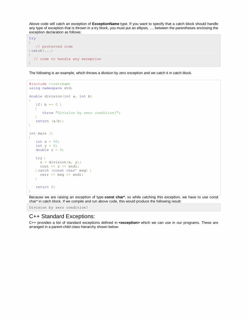
Above code will catch an exception of ExceptionName type. If you want to specify that a catch block should handle any type of exception that is thrown in a try block, you must put an ellipsis, ..., between the parentheses enclosing the exception declaration as follows:

try

{

// protected code

}catch(...)

{

// code to handle any exception

}

The following is an example, which throws a division by zero exception and we catch it in catch block.

#include <iostream>

using namespace std;

double division(int a, int b)

{

if( b == 0 )

{

throw "Division by zero condition!";

}

return (a/b);

}

int main ()

{

int x = 50;

int y = 0;

double z = 0;

try {

z = division(x, y);

cout << z << endl;

}catch (const char* msg) {

cerr << msg << endl;

}

return 0;

}

Because we are raising an exception of type const char*, so while catching this exception, we have to use const char* in catch block. If we compile and run above code, this would produce the following result:

Division by zero condition!

C++ Standard Exceptions: C++ provides a list of standard exceptions defined in <exception> which we can use in our programs. These are arranged in a parent-child class hierarchy shown below:

Here is the small description of each exception mentioned in the above hierarchy:

Exception Description

std::exception An exception and parent class of all the standard C++ exceptions.

std::bad_alloc This can be thrown by new.

std::bad_cast This can be thrown by dynamic_cast.

std::bad_exception This is useful device to handle unexpected exceptions in a C++ program

std::bad_typeid This can be thrown by typeid.

std::logic_error An exception that theoretically can be detected by reading the code.

std::domain_error This is an exception thrown when a mathematically invalid domain is used

std::invalid_argument This is thrown due to invalid arguments.

std::length_error This is thrown when a too big std::string is created

std::out_of_range This can be thrown by the at method from for example a std::vector and std::bitset<>::operator[]().

std::runtime_error An exception that theoretically can not be detected by reading the code.

std::overflow_error This is thrown if a mathematical overflow occurs.

std::range_error This is occured when you try to store a value which is out of range.

std::underflow_error This is thrown if a mathematical underflow occurs.

Define New Exceptions: You can define your own exceptions by inheriting and overriding exception class functionality. Following is the example, which shows how you can use std::exception class to implement your own exception in standard way:

#include <iostream>

#include <exception>

using namespace std;

struct MyException : public exception

{

const char * what () const throw ()

{

return "C++ Exception";

}

};

int main()

{

try

{

throw MyException();

}

catch(MyException& e)

{

std::cout << "MyException caught" << std::endl;

std::cout << e.what() << std::endl;

}

catch(std::exception& e)

{

//Other errors

}

}

This would produce the following result:

MyException caught

C++ Exception

Here, what() is a public method provided by exception class and it has been overridden by all the child exception classes. This returns the cause of an exception.

Standard libraries

The C++ Standard Library can be categorized into two parts:

The Standard Function Library: This library consists of general-purpose,stand-alone functions that are not part of any class. The function library is inherited from C.

The Object Oriented Class Library: This is a collection of classes and associated functions.

Standard C++ Library incorporates all the Standard C libraries also, with small additions and changes to support type safety.

The Standard Function Library:

The standard function library is divided into the following categories:

I/O

String and character handling

Mathematical

Time, date, and localization

Dynamic allocation

Miscellaneous

Wide-character functions

The Object Oriented Class Library:

Standard C++ Object Oriented Library defines an extensive set of classes that provide support for a number of common activities, including I/O, strings, and numeric processing. This library includes the following:

The Standard C++ I/O Classes

The String Class

The Numeric Classes

The STL Container Classes

The STL Algorithms

The STL Function Objects

The STL Iterators

The STL Allocators

The Localization library

Exception Handling Classes

Miscellaneous Support Library

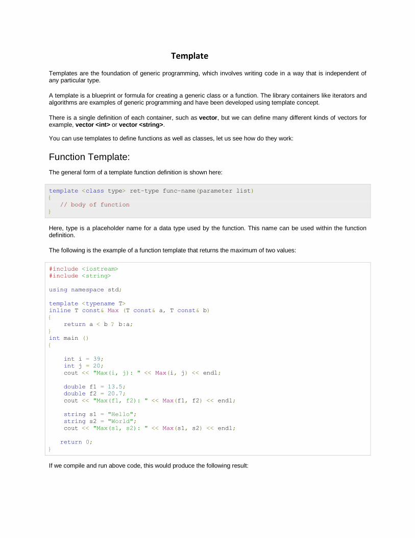
Template

Templates are the foundation of generic programming, which involves writing code in a way that is independent of any particular type.

A template is a blueprint or formula for creating a generic class or a function. The library containers like iterators and algorithms are examples of generic programming and have been developed using template concept.

There is a single definition of each container, such as vector, but we can define many different kinds of vectors for example, vector <int> or vector <string>.

You can use templates to define functions as well as classes, let us see how do they work:

Function Template:

The general form of a template function definition is shown here:

template <class type> ret-type func-name(parameter list)

{

// body of function

}

Here, type is a placeholder name for a data type used by the function. This name can be used within the function definition.

The following is the example of a function template that returns the maximum of two values:

#include <iostream>

#include <string>

using namespace std;

template <typename T>

inline T const& Max (T const& a, T const& b)

{

return a < b ? b:a;

}

int main ()

{

int i = 39;

int j = 20;

cout << "Max(i, j): " << Max(i, j) << endl;

double f1 = 13.5;

double f2 = 20.7;

cout << "Max(f1, f2): " << Max(f1, f2) << endl;

string s1 = "Hello";

string s2 = "World";

cout << "Max(s1, s2): " << Max(s1, s2) << endl;

return 0;

}

If we compile and run above code, this would produce the following result:

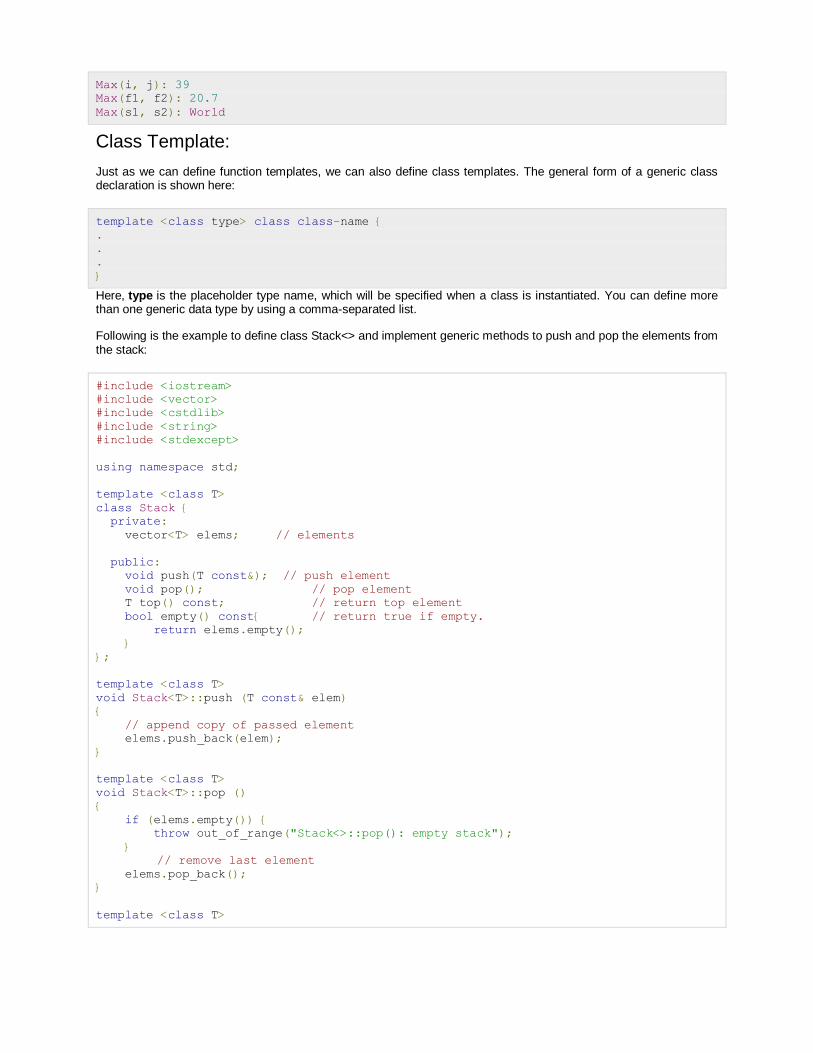
Max(i, j): 39

Max(f1, f2): 20.7

Max(s1, s2): World

Class Template:

Just as we can define function templates, we can also define class templates. The general form of a generic class declaration is shown here:

template <class type> class class-name {

.

.

.

}

Here, type is the placeholder type name, which will be specified when a class is instantiated. You can define more than one generic data type by using a comma-separated list.

Following is the example to define class Stack<> and implement generic methods to push and pop the elements from the stack:

#include <iostream>

#include <vector>

#include <cstdlib>

#include <string>

#include <stdexcept>

using namespace std;

template <class T>

class Stack {

private:

vector<T> elems; // elements

public:

void push(T const&); // push element

void pop(); // pop element

T top() const; // return top element

bool empty() const{ // return true if empty.

return elems.empty();

}

};

template <class T>

void Stack<T>::push (T const& elem)

{

// append copy of passed element

elems.push_back(elem);

}

template <class T>

void Stack<T>::pop ()

{

if (elems.empty()) {

throw out_of_range("Stack<>::pop(): empty stack");

}

// remove last element

elems.pop_back();

}

template <class T>

T Stack<T>::top () const

{

if (elems.empty()) {

throw out_of_range("Stack<>::top(): empty stack");

}

// return copy of last element

return elems.back();

}

int main()

{

try {

Stack<int> intStack; // stack of ints

Stack<string> stringStack; // stack of strings

// manipulate int stack

intStack.push(7);

cout << intStack.top() <<endl;

// manipulate string stack

stringStack.push("hello");

cout << stringStack.top() << std::endl;

stringStack.pop();

stringStack.pop();

}

catch (exception const& ex) {

cerr << "Exception: " << ex.what() <<endl;

return -1;

}

}

If we compile and run above code, this would produce the following result:

7

hello

Exception: Stack<>::pop(): empty stack

STL

The C++ STL (Standard Template Library) is a powerful set of C++ template classes to provides general-purpose templatized classes and functions that implement many popular and commonly used algorithms and data structures like vectors, lists, queues, and stacks.

At the core of the C++ Standard Template Library are following three well-structured components:

Component Description

Containers Containers are used to manage collections of objects of a certain kind. There are several different types of containers like deque, list, vector, map etc.

Algorithms Algorithms act on containers. They provide the means by which you will perform initialization, sorting, searching, and transforming of the contents of containers.

Iterators Iterators are used to step through the elements of collections of objects. These collections may be containers or subsets of containers.

We will discuss about all the three C++ STL components in next chapter while discussing C++ Standard Library. For now, keep in mind that all the three components have a rich set of pre-defined functions which help us in doing complicated tasks in very easy fashion.

Let us take the following program demonstrates the vector container (a C++ Standard Template) which is similar to an array with an exception that it automatically handles its own storage requirements in case it grows:

#include <iostream>

#include <vector>

using namespace std;

int main()

{

// create a vector to store int

vector<int> vec;

int i;

// display the original size of vec

cout << "vector size = " << vec.size() << endl;

// push 5 values into the vector

for(i = 0; i < 5; i++){

vec.push_back(i);

}

// display extended size of vec

cout << "extended vector size = " << vec.size() << endl;

// access 5 values from the vector

for(i = 0; i < 5; i++){

cout << "value of vec [" << i << "] = " << vec[i] << endl;

}

// use iterator to access the values

vector<int>::iterator v = vec.begin();

while( v != vec.end()) {

cout << "value of v = " << *v << endl;

v++;

}

return 0;

}

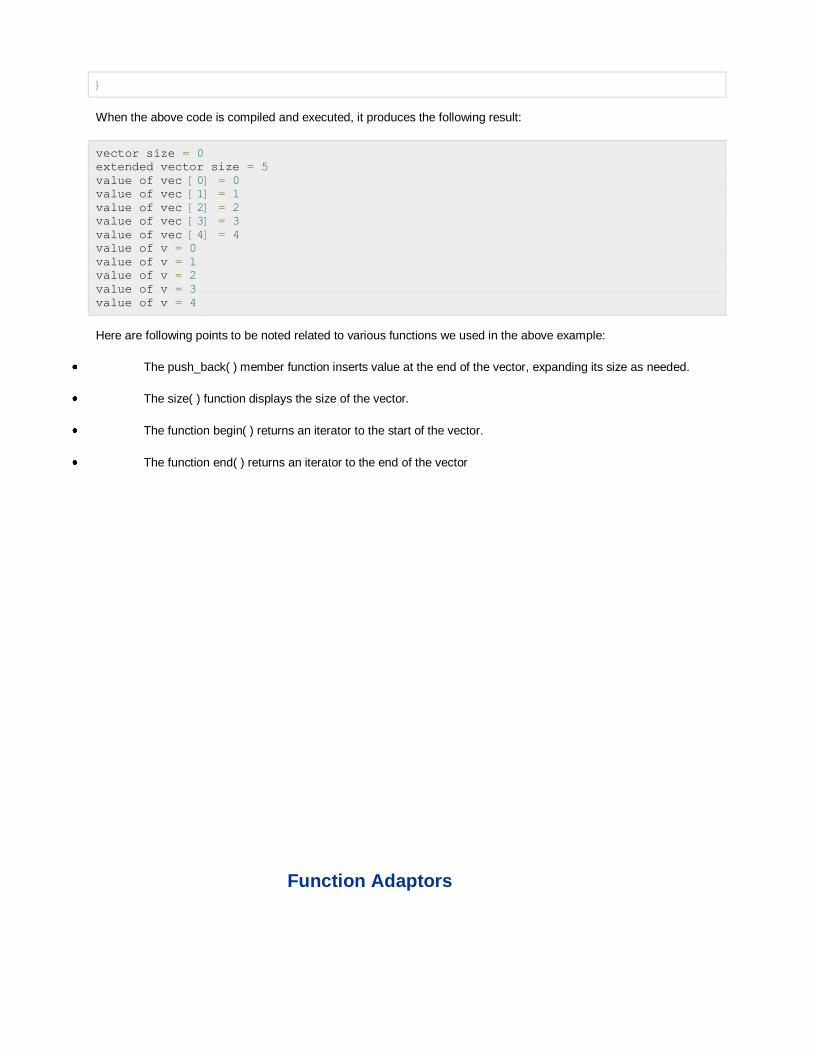
When the above code is compiled and executed, it produces the following result:

vector size = 0

extended vector size = 5

value of vec [0] = 0

value of vec [1] = 1

value of vec [2] = 2

value of vec [3] = 3

value of vec [4] = 4

value of v = 0

value of v = 1

value of v = 2

value of v = 3

value of v = 4

Here are following points to be noted related to various functions we used in the above example:

The push_back( ) member function inserts value at the end of the vector, expanding its size as needed.

The size( ) function displays the size of the vector.

The function begin( ) returns an iterator to the start of the vector.

The function end( ) returns an iterator to the end of the vector

Function Adaptors

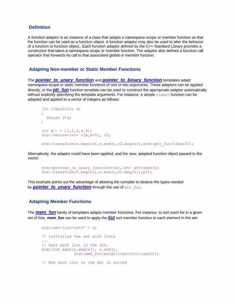
Definition

A function adaptor is an instance of a class that adapts a namespace-scope or member function so that the function can be used as a function object. A function adaptor may also be used to alter the behavior of a function or function object,. Each function adaptor defined by the C++ Standard Library provides a constructor that takes a namespace-scope or member function. The adaptor also defines a function call operator that forwards its call to that associated global or member function.

Adapting Non-member or Static Member Functions

The pointer_to_unary_function and pointer_to_binary_function templates adapt

namespace-scope or static member functions of one or two arguments. These adaptors can be applied

directly, or the ptr_fun function template can be used to construct the appropriate adaptor automatically

without explicitly specifying the template arguments. For instance, a simple times3 function can be

adapted and applied to a vector of integers as follows:

int times3(int x)

{

return 3*x;

}

int a[] = {1,2,3,4,5};

std::vector<int> v(a,a+5), v2;

std::transform(v.begin(),v.end(),v2.begin(),std::ptr_fun(times3));

Alternatively, the adaptor could have been applied, and the new, adapted function object passed to the vector:

std::pointer_to_unary_function<int,int> pf(times3);

std::transform(v.begin(),v.end(),v2.begin(),pf);

This example points out the advantage of allowing the compiler to deduce the types needed

by pointer_to_unary_function through the use of ptr_fun.

Adapting Member Functions

The mem_fun family of templates adapts member functions. For instance, to sort each list in a given

set of lists, mem_fun can be used to apply the list sort member function to each element in the set:

std::set<list<int>* > s;

// Initialize the set with lists

...

// Sort each list in the set.

std::for_each(s.begin(), s.end(),

std::mem_fun(&std::list<int>::sort));

// Now each list in the set is sorted

Using mem_fun is necessary because the generic sort algorithm requires random access iterators and

thus cannot be used on a list. It is also the simplest way to access any polymorphic characteristics of an

object held in a standard container. For instance, a virtual draw function might be invoked on a collection of objects that are all part of the canonical shape hierarchy like this:

// shape hierarchy

class shape {

virtual void draw() const;

};

class circle : public shape {

virtual void draw() const;

};

class square : public shape {

virtual void draw() const;

};

// Assemble a vector of shapes

const circle c;

const square s;

std::vector<shape*> v;

v.push_back(&s);

v.push_back(&c);

// Call draw on each one

std::for_each(v.begin(), v.end(), std::mem_fun(&shape::draw));

Each member function adaptor comes with an associated function template for convenience. The class template is the actual adaptor, while the function simplifies the use of the template by constructing instances of that class on the fly. For instance, in the previous example, a user could construct a const

_mem_fun_t, and pass that to the std::for_each() algorithm:

const_mem_fun_t<shape> mf(&shape::draw);

std::for_each(v.begin(), v.end(), mf);

Here again the mem_fun function template simplifies the use of the const_mem_fun_t adaptor by allowing the compiler to deduce the type needed by const_mem_fun_t. The fact that a const version of the function adaptor is needed (since the shapes are const) is obvious when the convenience function template is used.

The C++ Standard Library provides member function adaptors for functions with zero arguments as above and with one argument. Adaptors for member functions that operate on object references as opposed to object pointers such as those shown in the examples above are provided (mem_fun_ref_t), as are those that operate on pointers and references to const objects, respectively (const_mem_fun_t, const_mem_fun_ref_t). All of these adaptors can be easily extended to member

functions with more arguments.

Allocator

Allocators are one of the most mysterious parts of the C++ Standard library. Allocators are rarely used explicitly; the Standard doesn't make it clear when they should ever be used. Today's allocators are substantially different from those in the original STL proposal, and there were two other designs in between — all of which relied on language features that, until recently, were available on few compilers. The Standard appears to make promises about allocator

functionality with one hand and then take those promises away with the other.

This column will discuss what you can use allocators for and how you can define your own. I'm only going to discuss allocators as defined by the C++ Standard: bringing in pre-Standard designs, or workarounds for deficient compilers, would just add to the confusion.

When Not to Use Allocators

Allocators in the C++ Standard come in two pieces: a set of generic requirements, specified in 20.1.5 (Table 32), and the class std::allocator, specified in 20.4.1. We call a class an allocator if it conforms to the requirements of Table 32. The std::allocator class conforms to those requirements, so it is an allocator. It is the only predefined allocator class in the standard library.

Every C++ programmer already knows about dynamic memory allocation: you write new X to allocate memory and create a new object of type X, and you write delete p to destroy the object that p points to and return its memory. You might reasonably think that allocators have something to do with new and delete — but they don't. (The Standard describes ::operator new as an "allocation function," but, confusingly, that's not the same as an allocator.)

The most important fact about allocators is that they were intended for one purpose only: encapsulating the low-level details of STL containers' memory management. You shouldn't invoke allocator member functions in your own code, unless you're writing an STL container yourself. You shouldn't try to use allocators to implement operator new[]; that's not what they're for. If you aren't sure whether you need to use allocators, then you don't.

An allocator is a class with member functions allocate and deallocate, the rough equivalents of malloc and free. It also has helper functions for manipulating the memory that it allocated and typedefs that describe how to refer to the memory — names for pointer and reference types. If an STL container allocates all of its memory through a user-provided allocator (which the predefined STL containers all do; each of them has a template parameter that defaults tostd::allocator), you can control its memory management by providing your own allocator.

This flexibility is limited: a container still decides for itself how much memory it's going to ask for

and how the memory will be used. You get to control which low-level functions a container calls when it asks for more memory, but you can't use allocators to make a vector act like adeque. Sometimes, though, even this limited flexibility is useful. If you have a specialfast_allocator that allocates and deallocates memory quickly, for example (perhaps by giving up thread safety, or by using a small local heap), you can make the standard list class use it by writing std::list<T, fast_allocator<T> > instead of plain std::list<T>.

If this seems esoteric to you, you're right. There is no reason to use allocators in normal code.

Defining an Allocator

This already shows you something about allocators: they're templates. Allocators, like containers, have value types, and an allocator's value type must match the value type of the container it's used with. This can sometimes get ugly: map's value type is fairly complicated, so a map with an explicit

allocator involves expressions like std::map<K, V, fast_allocator<std::pair<const K, V> > >. (As usual, typedefs help.)

Let's start with a simple example. According to the C++ Standard, std::allocator is built on top of ::operator new. If you're using an automatic tool to trace memory usage, it's often more convenient to have something a bit simpler than std::allocator. We can use mallocinstead of ::operator new, and we can leave out the complicated performance optimizations that you'll find in a good implementation of std::allocator. We'll call this simple allocatormalloc_allocator.

Since the memory management in malloc_allocator is simple, we can focus on the boilerplate that's common to all STL allocators. First, some types: an allocator is a class template, and an instance of that template allocates memory specifically for objects of some type T. We provide a series of typedefs that describe how to refer to objects of that type: value_type for Titself, and others for the various flavors of pointers and references.

template <class T> class malloc_allocator

{

public:

typedef T value_type;

typedef value_type* pointer;

typedef const value_type* const_pointer;

typedef value_type& reference;

typedef const value_type& const_reference;

typedef std::size_t size_type;

typedef std::ptrdiff_t difference_type;

...

};

It's no accident that these types are so similar to those in an STL container: a container class

usually gets those types directly from its allocator.

Why so many typedefs? You might think that pointer is superfluous: it's just value_type*. Most of the time that's true, but you might occasionally want to define an unconventional allocator where pointer is some pointer-like class, or where it's some nonstandard vendor-

specific type like value_type __far*; allocators are a standard hook for nonstandard extensions. Unusual pointer types are also the reason for the address member function, which in malloc_allocator is just an alternate spelling for operator&:

template <class T> class malloc_allocator

{

public:

pointer address(reference x) const { return &x; }

const_pointer address(const_reference x) const {

return &x;

}

...

};

Now we can get to the real work: allocate and deallocate. They're straightforward, but they

don't look quite like malloc and free. We pass two arguments to allocate: the number of objects that we're allocating space for (max_size returns the largest request that might succeed), and, optionally, an address that can be used as a locality hint. A simple allocator like malloc_allocator makes no use of that hint, but an allocator designed for high performance might. The return value is a pointer to a block of memory that's large enough forn objects of type value_type and that has the correct alignment for that type.

We also pass two arguments to deallocate: a pointer, of course, but also an element count. A container has to keep track of sizes on its own; the size arguments to allocate anddeallocate must match. Again, this extra argument exists for reasons of performance, and again, malloc_allocator doesn't use it.

template <class T> class malloc_allocator

{

public:

pointer allocate(size_type n, const_pointer = 0) {

void* p = std::malloc(n * sizeof(T));

if (!p)

throw std::bad_alloc();

return static_cast<pointer>(p);

}

void deallocate(pointer p, size_type) {

std::free(p);

}

size_type max_size() const {

return static_cast<size_type>(-1) / sizeof(value_type);

}

...

};

The allocate and deallocate member functions deal with uninitialized memory; they don't construct or destroy objects. An expression like a.allocate(1) is more likemalloc(sizeof(int)) than like new int. Before using the memory you get from allocate, you have to create some objects in that memory; before returning that memory with deallocate, you have to destroy those objects.

C++ provides a mechanism for creating an object at a specific memory location: placement new. If you write new(p) T(a, b) then you are invoking T's constructor to create a new object, just as if you had written new T(a, b) or T t(a, b). The difference is that when you write new(p) T(a, b) you're specifying the location where that object is constructed: the address where p points. (Naturally, p has to point to a large enough region of memory, and it has to point to raw memory; you can't construct two different objects at the same address.) You can also call an object's destructor, without releasing any memory, by writing p->~T().

These features are rarely used, because usually memory allocation and initialization go together: it's inconvenient and dangerous to work with pointers to uninitialized memory. One of the few places where you need such low-level techniques is if you're writing a container class, so allocators decouple allocation from initialization. The member function construct performs placement new, and the member function destroy invokes the destructor.

template <class T> class malloc_allocator

{

public:

void construct(pointer p, const value_type& x) {

new(p) value_type(x);

}

void destroy(pointer p) { p->~value_type(); }

...

};

FILE HANDLING we have been using the iostream standard library, which provides cin and cout methods for reading from standard input and writing to standard output respectively.

This tutorial will teach you how to read and write from a file. This requires another standard C++ library called fstream, which defines three new data types:

Data Type Description

ofstream This data type represents the output file stream and is used to create files and to write information to files.

ifstream This data type represents the input file stream and is used to read information from files.

fstream This data type represents the file stream generally, and has the capabilities of both ofstream and ifstream which means it can create files, write information to files, and read information from files.

To perform file processing in C++, header files <iostream> and <fstream> must be included in your C++ source file.

Opening a File: A file must be opened before you can read from it or write to it. Either the ofstream or fstream object may be used to open a file for writing and ifstream object is used to open a file for reading purpose only.

Following is the standard syntax for open() function, which is a member of fstream, ifstream, and ofstream objects.

void open(const char *filename, ios::openmode mode);

Here, the first argument specifies the name and location of the file to be opened and the second argument of the open() member function defines the mode in which the file should be opened.

Mode Flag Description

ios::app Append mode. All output to that file to be appended to the end.

ios::ate Open a file for output and move the read/write control to the end of the file.

ios::in Open a file for reading.

ios::out Open a file for writing.

ios::trunc If the file already exists, its contents will be truncated before opening the file.

You can combine two or more of these values by ORing them together. For example if you want to open a file in write mode and want to truncate it in case it already exists, following will be the syntax:

ofstream outfile;

outfile.open("file.dat", ios::out | ios::trunc );

Similar way, you can open a file for reading and writing purpose as follows:

fstream afile;

afile.open("file.dat", ios::out | ios::in );

Closing a File

When a C++ program terminates it automatically closes flushes all the streams, release all the allocated memory and close all the opened files. But it is always a good practice that a programmer should close all the opened files before program termination.

Following is the standard syntax for close() function, which is a member of fstream, ifstream, and ofstream objects.

void close();

Writing to a File: While doing C++ programming, you write information to a file from your program using the stream insertion operator (<<) just as you use that operator to output information to the screen. The only difference is that you use an ofstream or fstream object instead of the cout object.

Reading from a File: You read information from a file into your program using the stream extraction operator (>>) just as you use that operator to input information from the keyboard. The only difference is that you use an ifstreamor fstream object instead of the cin object.

Read & Write Example:

Following is the C++ program which opens a file in reading and writing mode. After writing information inputted by the user to a file named afile.dat, the program reads information from the file and outputs it onto the screen:

#include <fstream>

#include <iostream>

using namespace std;

int main ()

{

char data[100];

// open a file in write mode.

ofstream outfile;

outfile.open("afile.dat");

cout << "Writing to the file" << endl;

cout << "Enter your name: ";

cin.getline(data, 100);

// write inputted data into the file.

outfile << data << endl;

cout << "Enter your age: ";

cin >> data;

cin.ignore();

// again write inputted data into the file.

outfile << data << endl;

// close the opened file.

outfile.close();

// open a file in read mode.

ifstream infile;

infile.open("afile.dat");

cout << "Reading from the file" << endl;

infile >> data;

// write the data at the screen.

cout << data << endl;

// again read the data from the file and display it.

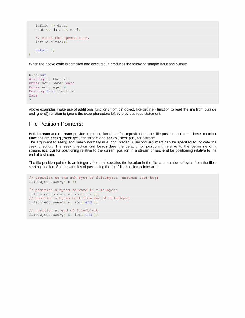
infile >> data;

cout << data << endl;

// close the opened file.

infile.close();

return 0;

}

When the above code is compiled and executed, it produces the following sample input and output:

$./a.out

Writing to the file

Enter your name: Zara

Enter your age: 9

Reading from the file

Zara

9

Above examples make use of additional functions from cin object, like getline() function to read the line from outside and ignore() function to ignore the extra characters left by previous read statement.

File Position Pointers:

Both istream and ostream provide member functions for repositioning the file-position pointer. These member functions are seekg ("seek get") for istream and seekp ("seek put") for ostream. The argument to seekg and seekp normally is a long integer. A second argument can be specified to indicate the seek direction. The seek direction can be ios::beg (the default) for positioning relative to the beginning of a stream, ios::cur for positioning relative to the current position in a stream or ios::end for positioning relative to the end of a stream.

The file-position pointer is an integer value that specifies the location in the file as a number of bytes from the file's starting location. Some examples of positioning the "get" file-position pointer are:

// position to the nth byte of fileObject (assumes ios::beg)

fileObject.seekg( n );

// position n bytes forward in fileObject

fileObject.seekg( n, ios::cur );

// position n bytes back from end of fileObject

fileObject.seekg( n, ios::end );

// position at end of fileObject

fileObject.seekg( 0, ios::end );

CS6301-PROGRAMMING & DATA STRUCTURES II

UNIT IV

Lecture Notes

AVL TREE

AVL tree (Adelson-Velskii and Landis' tree, named after the inventors) is a self-balancing binary

search tree. It was the first such data structure to be invented.[1] In an AVL tree, the heights of the

two child subtrees of any node differ by at most one; if at any time they differ by more than one,

rebalancing is done to restore this property.

• AVL trees are height-balanced binary search trees

• Balance factor of a node

› height(left subtree) - height(right subtree)

• An AVL tree has balance factor calculated at every node

› For every node, heights of left and right subtree can differ by no more than 1

› Store current heights in each node

Two types of rotation:

Single Rotation

Double Rotation

Single Rotation

LL Rotation

RR Rotation

Double Rotation

LR Rotation

RL Rotation

Single rotate (from the) left, on a left-left rotation

Double rotate (from the) left, on a left-right rotation

This diagram depicts the re-balance operation after an unbalancing left-right insertion.

Example:

1, 2, 3, 4, 5, 6, 7

Example:

50, 25, 10, 5, 7, 3, 30, 20, 8, 15

B-TREES

A m-way tree in which

The root has at least one key

Non-root nodes have at least m/2 subtrees (i.e., at least (m - 1)/2 keys)

All the empty subtrees (i.e., external nodes) are at the same level

Properties of B-Tree

1) All leaves are at same level.

2) A B-Tree is defined by the term minimum degree ‘t’. The value of t depends upon disk block

size.

3) Every node except root must contain at least t-1 keys. Root may contain minimum 1 key.

4) All nodes (including root) may contain at most 2t – 1 keys.

5) Number of children of a node is equal to the number of keys in it plus 1.

6) All keys of a node are sorted in increasing order. The child between two keys k1 and k2

contains all keys in range from k1 and k2.

7) B-Tree grows and shrinks from root which is unlike Binary Search Tree. Binary Search Trees

grow downward and also shrink from downward.

8) Like other balanced Binary Search Trees, time complexity to search, insert and delete is

O(Logn).

Following is an example B-Tree of minimum degree 3. Note that in practical B-Trees, the value

of minimum degree is much more than 3.

Search

Search is similar to search in Binary Search Tree. Let the key to be searched be k. We start from

root and recursively traverse down. For every visited non-leaf node, if the node has key, we

simply return the node. Otherwise we recur down to the appropriate child (The child which is

just before the first greater key) of the node. If we reach a leaf node and don’t find k in the leaf

node, we return NULL.

Add 19

Add 21

RED BLACK TREES

Red-Black Tree is a self-balancing Binary Search Tree (BST) where every node follows

following rules.

1) Every node has a color either red or black.

2) Root of tree is always black.

3) There are no two adjacent red nodes (A red node cannot have a red parent or red child).

4) Every path from root to a NULL node has same number of black nodes.

Insertion:

In AVL tree insertion, we used rotation as a tool to do balancing after insertion caused

imbalance. In Red-Black tree, we use two tools to do balancing.

1) Recoloring

2) Rotation

We try recoloring first, if recoloring doesn’t work, then we go for rotation. Following is detailed

algorithm. The algorithms has mainly two cases depending upon the color of uncle. If uncle is

red, we do recoloring. If uncle is black, we do rotations and/or recoloring.

Color of a NULL node is considered as BLACK.

Let x be the newly inserted node.

1) Perform standard BST insertion and make the color of newly inserted nodes as RED.

2) Do following if color of x’s parent is not BLACK or x is not root.

….a) If x’s uncle is RED (Grand parent must have been black from property 4)

……..(i) Change color of parent and uncle as BLACK.

……..(ii) color of grand parent as RED.

……..(iii) Change x = x’s grandparent, repeat steps 2 and 3 for new x.

….b) If x’s uncle is BLACK, then there can be four configurations for x, x’s parent (p) and x’s

grandparent (g) (This is similar to AVL Tree)

……..i) Left Left Case (p is left child of g and x is left child of p)

……..ii) Left Right Case (p is left child of g and x is right child of p)

……..iii) Right Right Case (Mirror of case a)

……..iv) Right Left Case (Mirror of case c)

3) If x is root, change color of x as BLACK (Black height of complete tree increases by 1).

Following are operations to be performed in four subcases when uncle is BLACK.

All four cases when Uncle is BLACK

Left Left Case (See g, p and x)

Left Right Case (See g, p and x)

Right Right Case (See g, p and x)

Right Left Case (See g, p and x)

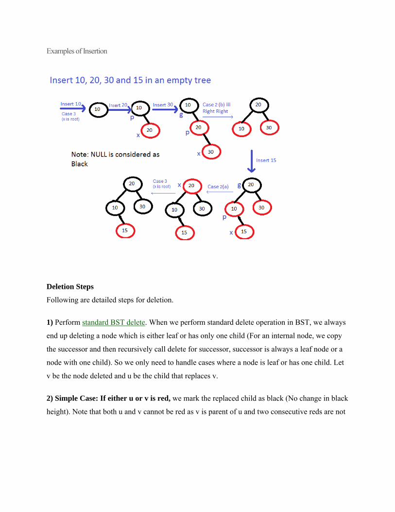
Examples of Insertion

Deletion Steps

Following are detailed steps for deletion.

1) Perform standard BST delete. When we perform standard delete operation in BST, we always

end up deleting a node which is either leaf or has only one child (For an internal node, we copy

the successor and then recursively call delete for successor, successor is always a leaf node or a

node with one child). So we only need to handle cases where a node is leaf or has one child. Let

v be the node deleted and u be the child that replaces v.

2) Simple Case: If either u or v is red, we mark the replaced child as black (No change in black

height). Note that both u and v cannot be red as v is parent of u and two consecutive reds are not

allowed in red-black tree.

3) If Both u and v are Black.

3.1) Color u as double black. Now our task reduces to convert this double black to single black.

Note that If v is leaf, then u is NULL and color of NULL is considered as black. So the deletion

of a black leaf also causes a double black.

3.2) Do following while the current node u is double black or it is not root. Let sibling of node

be s.

….(a): If sibling s is black and at least one of sibling’s children is red, perform rotation(s).

Let the red child of s be r. This case can be divided in four subcases depending upon positions of

s and r.

…………..(i) Left Left Case (s is left child of its parent and r is left child of s or both children of

s are red). This is mirror of right right case shown in below diagram.

…………..(ii) Left Right Case (s is left child of its parent and r is right child). This is mirror of

right left case shown in below diagram.

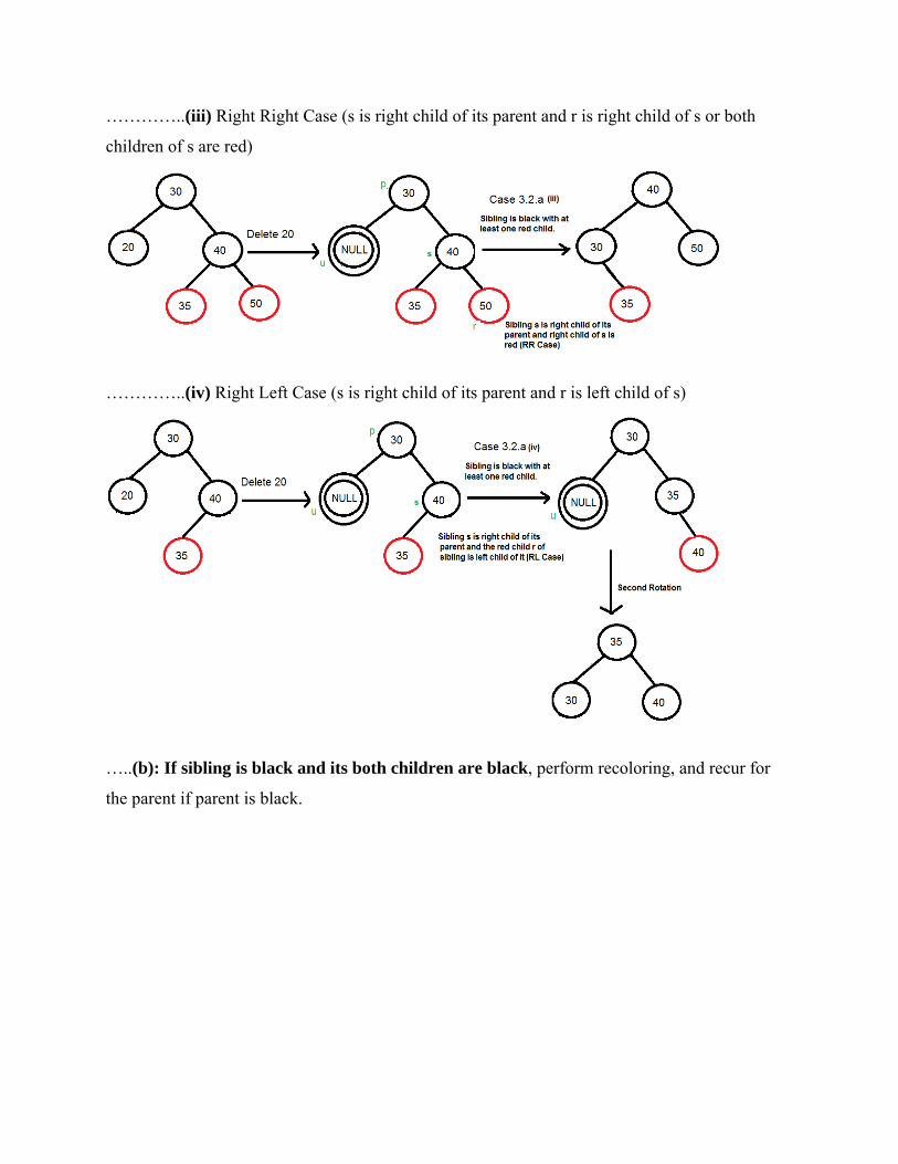
…………..(iii) Right Right Case (s is right child of its parent and r is right child of s or both

children of s are red)

…………..(iv) Right Left Case (s is right child of its parent and r is left child of s)

…..(b): If sibling is black and its both children are black, perform recoloring, and recur for

the parent if parent is black.

In this case, if parent was red, then we didn’t need to recur for prent, we can simply make it

black (red + double black = single black)

…..(c): If sibling is red, perform a rotation to move old sibling up, recolor the old sibling and

parent. The new sibling is always black (See the below diagram). This mainly converts the tree

to black sibling case (by rotation) and leads to case (a) or (b). This case can be divided in two

subcases.

…………..(i) Left Case (s is left child of its parent). This is mirror of right right case shown in

below diagram. We right rotate the parent p.

…………..(iii) Right Case (s is right child of its parent). We left rotate the parent p.

3.3) If u is root, make it single black and return (Black height of complete tree reduces by 1).

SPLAY TREES

A splay tree is a self-adjusting binary search tree with the additional property that recently

accessed elements are quick to access again. All normal operations on a binary search tree are

combined with one basic operation, called splaying. Splaying the tree for a certain element

rearranges the tree so that the element is placed at the root of the tree. One way to do this is to

first perform a standard binary tree search for the element in question, and then use tree rotations

in a specific fashion to bring the element to the top. Alternatively, a top-down algorithm can

combine the search and the tree reorganization into a single phase.

Rotation:

Zig zig rotation

Zag zag rotation

Zig zag rotation

Zag zig rotation

Zig zig rotation and Zag zag rotation

Zig zag rotation

Zag zig rotation

BINOMIAL HEAPS

A binomial heap is implemented as a collection of binomial trees (compare with a binary heap,

which has a shape of a single binary tree). A binomial tree is defined recursively:

A binomial tree of order 0 is a single node

A binomial tree of order k has a root node whose children are roots of binomial trees of

orders k−1, k−2, ..., 2, 1, 0 (in this order).

A binomial heap is implemented as a set of binomial trees that satisfy the binomial heap

Properties:

Each binomial tree in a heap obeys the minimum-heap property: the key of a node is

greater than or equal to the key of its parent.

There can only be either one or zero binomial trees for each order, including zero order.

The first property ensures that the root of each binomial tree contains the smallest key in the tree,

which applies to the entire heap.

The second property implies that a binomial heap with n nodes consists of at most log n + 1

binomial trees. In fact, the number and orders of these trees are uniquely determined by the

number of nodes n: each binomial tree corresponds to one digit in the binary representation of

number n. For example number 13 is 1101 in binary, , and thus a binomial heap

with 13 nodes will consist of three binomial trees of orders 3, 2, and 0 (see figure below).

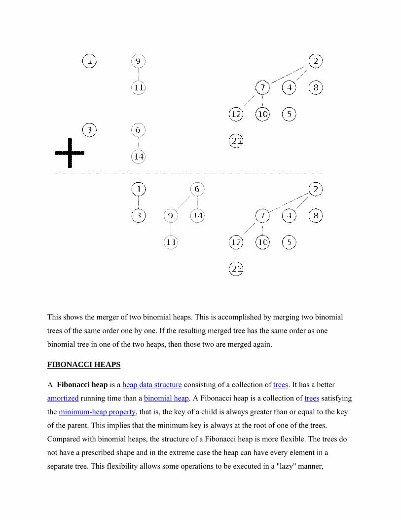
This shows the merger of two binomial heaps. This is accomplished by merging two binomial

trees of the same order one by one. If the resulting merged tree has the same order as one

binomial tree in one of the two heaps, then those two are merged again.

FIBONACCI HEAPS

A Fibonacci heap is a heap data structure consisting of a collection of trees. It has a better

amortized running time than a binomial heap. A Fibonacci heap is a collection of trees satisfying

the minimum-heap property, that is, the key of a child is always greater than or equal to the key

of the parent. This implies that the minimum key is always at the root of one of the trees.

Compared with binomial heaps, the structure of a Fibonacci heap is more flexible. The trees do

not have a prescribed shape and in the extreme case the heap can have every element in a

separate tree. This flexibility allows some operations to be executed in a "lazy" manner,

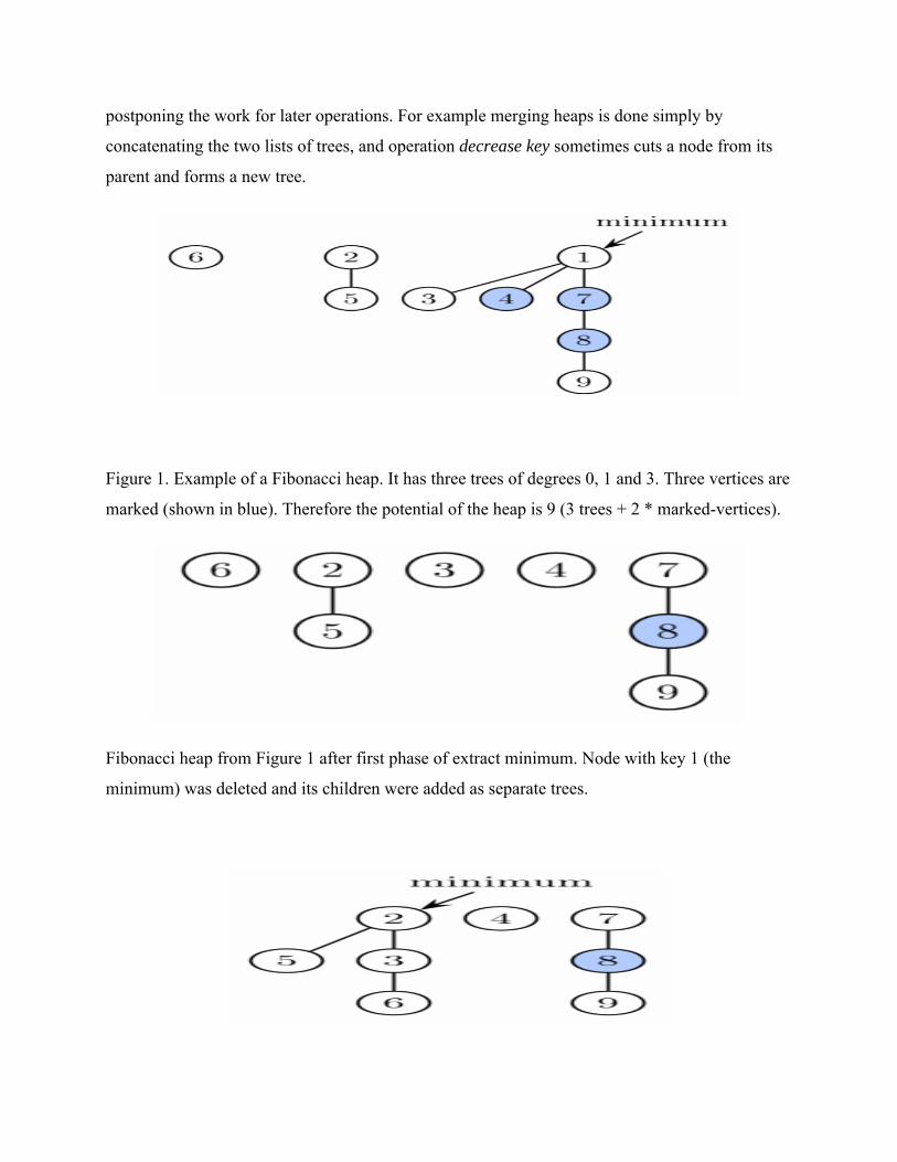
postponing the work for later operations. For example merging heaps is done simply by

concatenating the two lists of trees, and operation decrease key sometimes cuts a node from its

parent and forms a new tree.

Figure 1. Example of a Fibonacci heap. It has three trees of degrees 0, 1 and 3. Three vertices are

marked (shown in blue). Therefore the potential of the heap is 9 (3 trees + 2 * marked-vertices).

Fibonacci heap from Figure 1 after first phase of extract minimum. Node with key 1 (the

minimum) was deleted and its children were added as separate trees.

Fibonacci heap from Figure 1 after extract minimum is completed. First, nodes 3 and 6 are linked

together. Then the result is linked with tree rooted at node 2. Finally, the new minimum is found.

Fibonacci heap from Figure 1 after decreasing key of node 9 to 0. This node as well as its two

marked ancestors are cut from the tree rooted at 1 and placed as new roots.

DISJOINT SETS

Some applications involve grouping n distinct objects into a collection of disjoint sets. Two

important operations are then finding which set a given object belongs to and uniting the two

sets.

A disjoint set data structure maintains a collection S={ S1 , S2 ,…, Sk } of disjoint dynamic sets.

Each set is identified by a representative, which usually is a member in the set.

1 Operations on Sets

Let x be an object. We wish to support the following operations.

MAKE-SET( x) creates a new set whose only member is pointed by x; Note that x is not in the

other sets.

UNION( x,y) unites two dynamic sets containing objects x and y, say Sx and Sy , into a new set

that Sx∪Sy , assuming that Sx ∩ Sy =∅;

FIND-SET( x) returns a pointer to the representative of the set containing x.

INSERT(a,S) inserts an object a to S, and returns S∪{a}.

DELETE(a,S) deletes an object a from S, and returns S-{a}.

SPLIT(a,S) partitions the objects of S into two sets S1 and S2 such that S1 ={b | b≤a b∈S},

and S2 =S- S1 .

MINIMUM( S) returns the minimum object in S.

2 Applications of Disjoint-set Data Structures

Here we show two application examples.

Connected components (CCs)

Minimum Spanning Trees (MSTs)

2.1 Algorithm for Connected Components

CONNECTED-COMPONENTS (G)

1 for each v∈V

2 do MAKE-SET (v)

3 for every edge (u,v)∈E

4 do if FIND-SET (u) ≠ FIND-SET (v)

5 then UNION (u,v)

SAME-COMPONENTS (u,v)

1 if FIND-SET (u) = FIND-SET (v)

2 then return TRUE

3 return FALSE

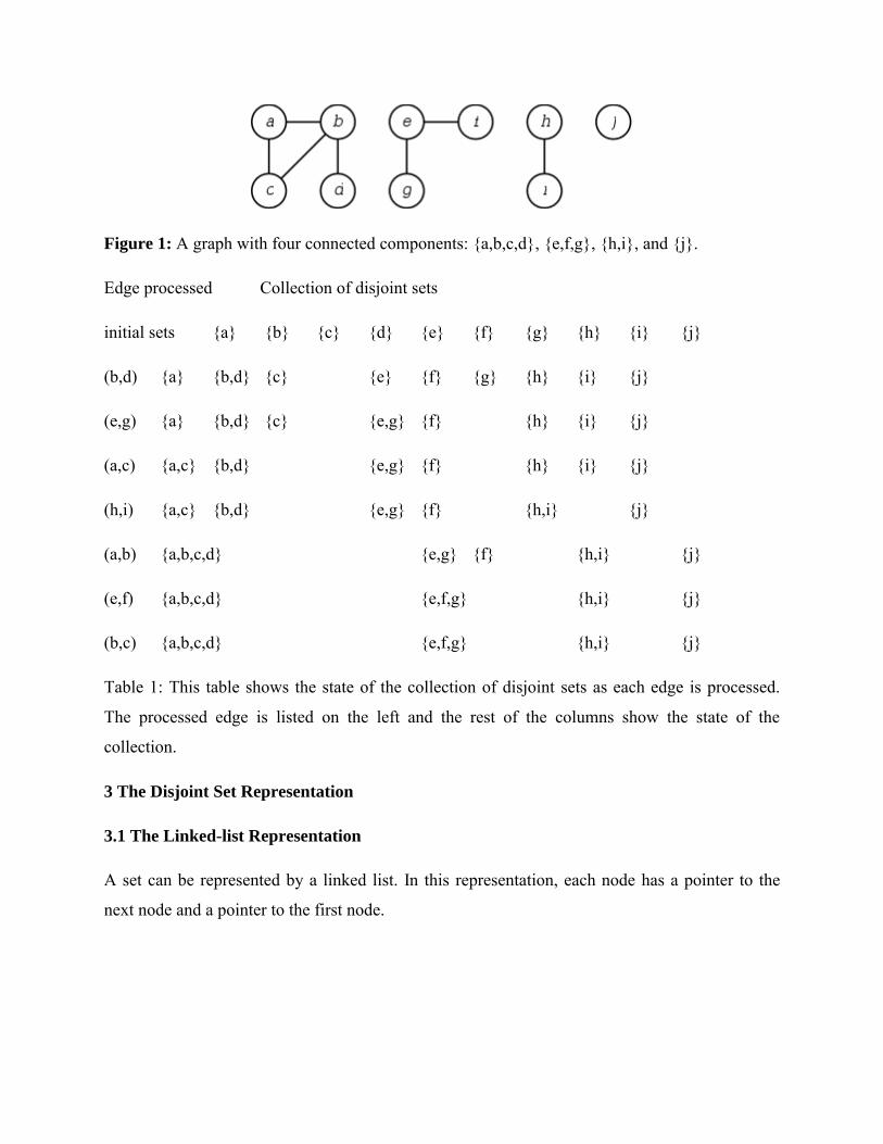
Figure 1: A graph with four connected components: {a,b,c,d}, {e,f,g}, {h,i}, and {j}.

Edge processed Collection of disjoint sets

initial sets {a} {b} {c} {d} {e} {f} {g} {h} {i} {j}

(b,d) {a} {b,d} {c} {e} {f} {g} {h} {i} {j}

(e,g) {a} {b,d} {c} {e,g} {f} {h} {i} {j}

(a,c) {a,c} {b,d} {e,g} {f} {h} {i} {j}

(h,i) {a,c} {b,d} {e,g} {f} {h,i} {j}

(a,b) {a,b,c,d} {e,g} {f} {h,i} {j}

(e,f) {a,b,c,d} {e,f,g} {h,i} {j}

(b,c) {a,b,c,d} {e,f,g} {h,i} {j}

Table 1: This table shows the state of the collection of disjoint sets as each edge is processed.

The processed edge is listed on the left and the rest of the columns show the state of the

collection.

3 The Disjoint Set Representation

3.1 The Linked-list Representation

A set can be represented by a linked list. In this representation, each node has a pointer to the

next node and a pointer to the first node.

Figure 2: Linked-list representation. Each disjoint set can be represented by a linked-list. Each

node has a pointer to the head node and a pointer to the next node.

Consider the following operation sequence:

MAKE-SET ( x1 ),

MAKE-SET ( x2 ),

:,

MAKE-SET ( xn-1 ),

MAKE-SET ( xn ),

UNION ( x1 , x2 ),

UNION ( x2 , x3 ),

:,

UNION ( xn-1 , xn ).

What's the total time complexity of the above operations?

A weighted-union heuristic: Assume that the representative of each set maintains the number of

objects in the set, and always merge the smaller list to the larger list, then

Theorem: Using the linked list representation of disjoint sets and the weighted-union heuristic, a

sequence of m MAKE-SET, Union, and Find_Set operations, n of which are MAKE-SET, takes

O(m+nlogn) time.

Hint: observe that for any k≤n, after x's representative pointer has been updated ⌈logk⌉ times, the

resulting set containing x must have at least k members.

4 Disjoint Set Forests

A faster implementation of disjoint sets is through the rooted trees, with each node containing

one member and each tree representing one set. Each member in the tree has only one parent.

Figure 3: Rooted tree representation of disjoint sets. Each tree has a "representative" h for the

left tree and a for the right tree.

4.1 The Heuristics for Disjoint Set Operations

union by rank.

path compression

The idea of union by rank is to make the root of the tree with fewer nodes point to the root of

the tree with more nodes. Rather than explicitly keeping track of the size of the subtree rooted at

each node, for each node we maintain a rank that approximates the logarithm of the subtree size

and is also an upper bound on the height of the node.

Time complexity: O(mlogn), assuming that there are m union operations.

Path compression is quite simple and very effective. We use this approach during FIND-SET

operations to make each node on the path point directly to the root. Path compression does not

change any ranks.

Figure 4: Path compression takes place during the FIND-SET operation. This works by

recursing from the given input node up to the root of the tree, forming a path. Then the root is

returned and assigned as the parent for each node in path. The parent of c after FIND-SET (c) is

h.

Time complexity: Θ(f log1+f/n) n) if f≥n and Θ(n+flogn) otherwise, assume that there are n

MAKE-SET operations and f FIND-SET operations.

MAKE-SET (x)

1 p[x] ← x

2 rank[x] ← 0

FIND-SET (x)

1 if x≠p[x]

2 then p[x] ← FIND-SET (p[x])

3 return p[x]

UNION (x,y)

1 LINK( FIND-SET (x), FIND-SET (y))

LINK (x,y)

1 if rank[x]>rank[y]

2 then p[y] ← x

3 else p[x] ← y

4 if rank[x]=rank[y]

5 then rank[y] ← rank[y]+1

where rank[x] is the height of x in the tree. If both of the above methods are used together, the

time complexity is O(mα(m,n)).

The Rank properties

rank[x]≤rank[p[x]]

for any tree root x, size(x)≥ 2rank[x] (Link operation)

for any integer r, there are at most n/ 2r nodes of rank r

each node has rank at most ⌊logn⌋, assuming there are at n objects involved.

AMORTIZED ANALYSIS- ACCOUNTING METHOD- POTENTIAL METHOD-

AGGREGATE ANALYSIS

Amortized Analysis

-After discussing algorithm design techniques (Dynamic programming and Greedy algorithms)

we now return to data structures and discuss a new analysis method|Amortized analysis.

_ Until now we have seen a number of data structures and analyzed the worst-case running

time of each individual operation.

_ Sometimes the cost of an operation vary widely, so that that worst-case running time is not

really a good cost measure.

_ Similarly, sometimes the cost of every single operation is not so important

{ the total cost of a series of operations are more important (e.g when using priority queue

to sort)

_ We want to analyze running time of one single operation averaged over a sequence of

operations

-Note: We are not interested in an average case analyses that depends on some input

distribution or random choices made by algorithm.

_ To capture this we define amortized time.

If any sequence of n operations on a data structure takes _ T(n) time,

the amortized time per operation is T(n)=n

- Equivalently, if the amortized time of one operation is U(n), then any

sequence of n operations takes n _ U(n) time.

_ Again keep in mind: \Average" is over a sequence of operations for any sequence

{ not average for some input distribution (as in quick-sort)

{ not average over random choices made by algorithm (as in skip-lists)

Potential Method

_ In the two previous examples we basically just did a careful analysis to get O(n) bounds

leading to O(1) amortized bounds.

-book calls this aggregate analysis.

_ In aggregate analysis, all operations have the same amortized cost (total cost divided by n)

other and more sophisticated amortized analysis methods allow different operations to

have different amortized costs.

_ Potential method:

- Idea is to overcharge some operations and store the overcharge as credits/potential which

can then help pay for later operations (making them cheaper).

{ Leads to equivalent but slightly different definition of amortized time.

_ Consider performing n operations on an initial data structure D0

- Di is data structure after ith operation, i = 1; 2; : : : ; n.

-ci is actual cost (time) of ith operation, i = 1; 2; : : : ; n.

PROGRAMMING & DATA STRUCTURESII

UNIT V

Lecture Notes

REPRESENTATION OF GRAPHS

Graph and its representations

Graph is a data structure that consists of following two components:

1. A finite set of vertices also called as nodes.

2. A finite set of ordered pair of the form (u, v) called as edge. The pair is ordered because (u, v)

is not same as (v, u) in case of directed graph(di-graph). The pair of form (u, v) indicates that

there is an edge from vertex u to vertex v. The edges may contain weight/value/cost.

Graphs are used to represent many real life applications: Graphs are used to represent networks.

The networks may include paths in a city or telephone network or circuit network. Graphs are

also used in social networks like linkedIn, facebook. For example, in facebook, each person is

represented with a vertex(or node). Each node is a structure and contains information like person

id, name, gender and locale. This can be easily viewed by

http://graph.facebook.com/barnwal.aashish where barnwal.aashish is the profile name. See this

for more applications of graph.

Following is an example undirected graph with 5 vertices.

Following two are the most commonly used representations of graph.

1. Adjacency Matrix

2. Adjacency List

There are other representations also like, Incidence Matrix and Incidence List. The choice of the

graph representation is situation specific. It totally depends on the type of operations to be

performed and ease of use.

Adjacency Matrix:

Adjacency Matrix is a 2D array of size V x V where V is the number of vertices in a graph. Let

the 2D array be adj[][], a slot adj[i][j] = 1 indicates that there is an edge from vertex i to vertex j.

Adjacency matrix for undirected graph is always symmetric. Adjacency Matrix is also used to

represent weighted graphs. If adj[i][j] = w, then there is an edge from vertex i to vertex j with

weight w.

The adjacency matrix for the above example graph is:

Adjacency Matrix Representation of the above graph

Pros: Representation is easier to implement and follow. Removing an edge takes O(1) time.

Queries like whether there is an edge from vertex ‘u’ to vertex ‘v’ are efficient and can be done

O(1).

Cons: Consumes more space O(V^2). Even if the graph is sparse(contains less number of edges),

it consumes the same space. Adding a vertex is O(V^2) time.

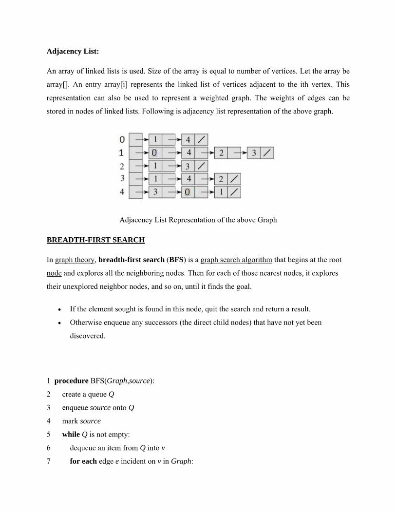
Adjacency List:

An array of linked lists is used. Size of the array is equal to number of vertices. Let the array be

array[]. An entry array[i] represents the linked list of vertices adjacent to the ith vertex. This

representation can also be used to represent a weighted graph. The weights of edges can be

stored in nodes of linked lists. Following is adjacency list representation of the above graph.

Adjacency List Representation of the above Graph

BREADTH-FIRST SEARCH

In graph theory, breadth-first search (BFS) is a graph search algorithm that begins at the root

node and explores all the neighboring nodes. Then for each of those nearest nodes, it explores

their unexplored neighbor nodes, and so on, until it finds the goal.

If the element sought is found in this node, quit the search and return a result.

Otherwise enqueue any successors (the direct child nodes) that have not yet been

discovered.

1 procedure BFS(Graph,source):

2 create a queue Q

3 enqueue source onto Q

4 mark source

5 while Q is not empty:

6 dequeue an item from Q into v

7 for each edge e incident on v in Graph:

8 let w be the other end of e

9 if w is not marked:

10 mark w

11 enqueue w onto Q

DEPTH-FIRST SEARCH (DFS)

Depth-first search, or DFS, is a way to traverse the graph. Initially it allows visiting vertices of

the graph only, but there are hundreds of algorithms for graphs, which are based on DFS.

Therefore, understanding the principles of depth-first search is quite important to move ahead

into the graph theory. The principle of the algorithm is quite simple: to go forward (in depth)

while there is such possibility, otherwise to backtrack.

Algorithm

In DFS, each vertex has three possible colors representing its state:

white: vertex is unvisited;

gray: vertex is in progress;

black: DFS has finished processing the vertex.

NB. For most algorithms boolean classification unvisited / visited is quite enough, but we

show general case here.

Initially all vertices are white (unvisited). DFS starts in arbitrary vertex and runs as follows:

1. Mark vertex u as gray (visited).

2. For each edge (u, v), where u is white, run depth-first search for u recursively.

3. Mark vertex u as black and backtrack to the parent.

Example. Traverse a graph shown below, using DFS. Start from a vertex with number 1.

Source graph.

Mark a vertex 1 as gray.

There is an edge (1, 4) and a vertex 4 is

unvisited. Go there.

Mark the vertex 4 as gray.

There is an edge (4, 2) and vertex a 2 is

unvisited. Go there.

Mark the vertex 2 as gray.

There is an edge (2, 5) and a vertex 5 is

unvisited. Go there.

Mark the vertex 5 as gray.

There is an edge (5, 3) and a vertex 3 is

unvisited. Go there.

Mark the vertex 3 as gray.

There are no ways to go from the vertex

3. Mark it as black and backtrack to the

vertex 5.

There is an edge (5, 4), but the vertex 4 is

gray.

There are no ways to go from the vertex

5. Mark it as black and backtrack to the

vertex 2.

There are no more edges, adjacent to

vertex 2. Mark it as black and backtrack

to the vertex 4.

There is an edge (4, 5), but the vertex 5 is

black.

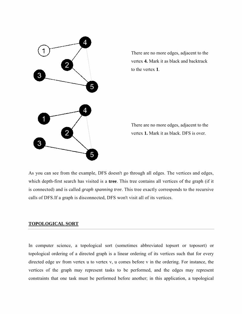
There are no more edges, adjacent to the

vertex 4. Mark it as black and backtrack

to the vertex 1.

There are no more edges, adjacent to the

vertex 1. Mark it as black. DFS is over.

As you can see from the example, DFS doesn't go through all edges. The vertices and edges,

which depth-first search has visited is a tree. This tree contains all vertices of the graph (if it

is connected) and is called graph spanning tree. This tree exactly corresponds to the recursive

calls of DFS.If a graph is disconnected, DFS won't visit all of its vertices.

TOPOLOGICAL SORT

In computer science, a topological sort (sometimes abbreviated topsort or toposort) or

topological ordering of a directed graph is a linear ordering of its vertices such that for every

directed edge uv from vertex u to vertex v, u comes before v in the ordering. For instance, the

vertices of the graph may represent tasks to be performed, and the edges may represent

constraints that one task must be performed before another; in this application, a topological

ordering is just a valid sequence for the tasks. A topological ordering is possible if and only if the

graph has no directed cycles, that is, if it is a directed acyclic graph (DAG). Any DAG has at

least one topological ordering, and algorithms are known for constructing a topological ordering

of any DAG in linear time.

The canonical application of topological sorting (topological order) is in scheduling a sequence

of jobs or tasks based on their dependencies; topological sorting algorithms were first studied in

the early 1960s in the context of the PERT technique for scheduling in project management

(Jarnagin 1960). The jobs are represented by vertices, and there is an edge from x to y if job x

must be completed before job y can be started (for example, when washing clothes, the washing

machine must finish before we put the clothes to dry). Then, a topological sort gives an order in

which to perform the jobs.

In computer science, applications of this type arise in instruction scheduling, ordering of formula

cell evaluation when recomputing formula values in spreadsheets, logic synthesis, determining

the order of compilation tasks to perform in makefiles, data serialization, and resolving symbol

dependencies in linkers. It is also used to decide in which order to load tables with foreign keys

in databases.

The graph shown to the left has many valid topological sorts, including:

7, 5, 3, 11, 8, 2, 9, 10 (visual left-to-right, top-to-bottom)

3, 5, 7, 8, 11, 2, 9, 10 (smallest-numbered available vertex first)

5, 7, 3, 8, 11, 10, 9, 2 (fewest edges first)

7, 5, 11, 3, 10, 8, 9, 2 (largest-numbered available vertex first)

7, 5, 11, 2, 3, 8, 9, 10 (attempting top-to-bottom, left-to-right)

3, 7, 8, 5, 11, 10, 2, 9 (arbitrary)

Algorithms

The usual algorithms for topological sorting have running time linear in the number of nodes

plus the number of edges, asymptotically, O(\left|{V}\right| + \left|{E}\right|).

One of these algorithms, first described by Kahn (1962), works by choosing vertices in the same

order as the eventual topological sort. First, find a list of "start nodes" which have no incoming

edges and insert them into a set S; at least one such node must exist in an acyclic graph. Then:

L ← Empty list that will contain the sorted elements

S ← Set of all nodes with no incoming edges

while S is non-empty do

remove a node n from S

add n to tail of L

for each node m with an edge e from n to m do

remove edge e from the graph

if m has no other incoming edges then

insert m into S

if graph has edges then

return error (graph has at least one cycle)

else

return L (a topologically sorted order)

If the graph is a DAG, a solution will be contained in the list L (the solution is not necessarily

unique). Otherwise, the graph must have at least one cycle and therefore a topological sorting is

impossible.

Reflecting the non-uniqueness of the resulting sort, the structure S can be simply a set or a queue

or a stack. Depending on the order that nodes n are removed from set S, a different solution is

created. A variation of Kahn's algorithm that breaks ties lexicographically forms a key

component of the Coffman–Graham algorithm for parallel scheduling and layered graph

drawing.

An alternative algorithm for topological sorting is based on depth-first search. The algorithm

loops through each node of the graph, in an arbitrary order, initiating a depth-first search that

terminates when it hits any node that has already been visited since the beginning of the

topological sort:

L ← Empty list that will contain the sorted nodes

while there are unmarked nodes do

select an unmarked node n

visit(n)

function visit(node n)

if n has a temporary mark then stop (not a DAG)

if n is not marked (i.e. has not been visited yet) then

mark n temporarily

for each node m with an edge from n to m do

visit(m)

mark n permanently

unmark n temporarily

add n to head of L

Each node n gets prepended to the output list L only after considering all other nodes on which n

depends (all ancestral nodes of n in the graph). Specifically, when the algorithm adds node n, we

are guaranteed that all nodes on which n depends are already in the output list L: they were

added to L either by the preceding recursive call to visit(), or by an earlier call to visit(). Since

each edge and node is visited once, the algorithm runs in linear time. This depth-first-search-

based algorithm is the one described by Cormen et al. (2001); it seems to have been first

described in print by Tarjan (1976).

MINIMUM SPANNING TREES

The Minimum Spanning Tree for a given graph is the Spanning Tree of minimum cost for that

graph.

Algorithms for Obtaining the Minimum Spanning Tree

• Kruskal's Algorithm

• Prim's Algorithm

Kruskal's Algorithm

This algorithm creates a forest of trees. Initially the forest consists of n single node trees (and no

edges). At each step, we add one edge (the cheapest one) so that it joins two trees together. If it

were to form a cycle, it would simply link two nodes that were already part of a single connected

tree, so that this edge would not be needed.

The steps are:

1. The forest is constructed - with each node in a separate tree.

2. The edges are placed in a priority queue.

3. Until we've added n-1 edges,

1. Extract the cheapest edge from the queue,

2. If it forms a cycle, reject it,

3. Else add it to the forest. Adding it to the forest will join two trees together.

Every step will have joined two trees in the forest together, so that at the end, there will only be

one tree in T.

Prim's Algorithm

This algorithm starts with one node. It then, one by one, adds a node that is unconnected to the

new graph to the new graph, each time selecting the node whose connecting edge has the

smallest weight out of the available nodes’ connecting edges.

The steps are:

1. The new graph is constructed - with one node from the old graph.

2. While new graph has fewer than n nodes,

1. Find the node from the old graph with the smallest connecting edge to the new graph,

2. Add it to the new graph

Every step will have joined one node, so that at the end we will have one graph with all the

nodes and it will be a minimum spanning tree of the original graph.

SHORTEST PATH ALGORITHM

Dijkstra’s algorithm

Given a graph and a source vertex in graph, find shortest paths from source to all vertices in the

given graph.

Dijkstra’s algorithm is very similar to Prim’s algorithm for minimum spanning tree. Like Prim’s

MST, we generate a SPT (shortest path tree) with given source as root. We maintain two sets,

one set contains vertices included in shortest path tree, other set includes vertices not yet

included in shortest path tree. At every step of the algorithm, we find a vertex which is in the

other set (set of not yet included) and has minimum distance from source.

Below are the detailed steps used in Dijkstra’s algorithm to find the shortest path from a single

source vertex to all other vertices in the given graph.

Algorithm

1) Create a set sptSet (shortest path tree set) that keeps track of vertices included in shortest path

tree, i.e., whose minimum distance from source is calculated and finalized. Initially, this set is

empty.

2) Assign a distance value to all vertices in the input graph. Initialize all distance values as

INFINITE. Assign distance value as 0 for the source vertex so that it is picked first.

3) While sptSet doesn’t include all vertices

….a) Pick a vertex u which is not there in sptSetand has minimum distance value.

….b) Include u to sptSet.

….c) Update distance value of all adjacent vertices of u. To update the distance values, iterate

through all adjacent vertices. For every adjacent vertex v, if sum of distance value of u (from

source) and weight of edge u-v, is less than the distance value of v, then update the distance

value of v.

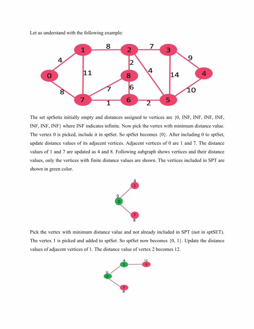
Let us understand with the following example:

The set sptSetis initially empty and distances assigned to vertices are {0, INF, INF, INF, INF,

INF, INF, INF} where INF indicates infinite. Now pick the vertex with minimum distance value.

The vertex 0 is picked, include it in sptSet. So sptSet becomes {0}. After including 0 to sptSet,

update distance values of its adjacent vertices. Adjacent vertices of 0 are 1 and 7. The distance

values of 1 and 7 are updated as 4 and 8. Following subgraph shows vertices and their distance

values, only the vertices with finite distance values are shown. The vertices included in SPT are

shown in green color.

Pick the vertex with minimum distance value and not already included in SPT (not in sptSET).

The vertex 1 is picked and added to sptSet. So sptSet now becomes {0, 1}. Update the distance

values of adjacent vertices of 1. The distance value of vertex 2 becomes 12.

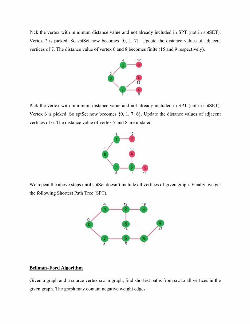
Pick the vertex with minimum distance value and not already included in SPT (not in sptSET).

Vertex 7 is picked. So sptSet now becomes {0, 1, 7}. Update the distance values of adjacent

vertices of 7. The distance value of vertex 6 and 8 becomes finite (15 and 9 respectively).

Pick the vertex with minimum distance value and not already included in SPT (not in sptSET).

Vertex 6 is picked. So sptSet now becomes {0, 1, 7, 6}. Update the distance values of adjacent

vertices of 6. The distance value of vertex 5 and 8 are updated.

We repeat the above steps until sptSet doesn’t include all vertices of given graph. Finally, we get

the following Shortest Path Tree (SPT).

Bellman–Ford Algorithm

Given a graph and a source vertex src in graph, find shortest paths from src to all vertices in the

given graph. The graph may contain negative weight edges.

We have discussed Dijkstra’s algorithm for this problem. Dijksra’s algorithm is a Greedy

algorithm and time complexity is O(VLogV) (with the use of Fibonacci heap). Dijkstra doesn’t

work for Graphs with negative weight edges, Bellman-Ford works for such graphs. Bellman-

Ford is also simpler than Dijkstra and suites well for distributed systems. But time complexity of

Bellman-Ford is O(VE), which is more than Dijkstra.

Algorithm

Following are the detailed steps.

Input: Graph and a source vertex src

Output: Shortest distance to all vertices from src. If there is a negative weight cycle, then shortest

distances are not calculated, negative weight cycle is reported.

1) This step initializes distances from source to all vertices as infinite and distance to source

itself as 0. Create an array dist[] of size |V| with all values as infinite except dist[src] where src is

source vertex.

2) This step calculates shortest distances. Do following |V|-1 times where |V| is the number of

vertices in given graph.

…..a) Do following for each edge u-v

………………If dist[v] >dist[u] + weight of edge uv, then update dist[v]

………………….dist[v] = dist[u] + weight of edge uv

3) This step reports if there is a negative weight cycle in graph. Do following for each edge u-v

……If dist[v] >dist[u] + weight of edge uv, then “Graph contains negative weight cycle”

The idea of step 3 is, step 2 guarantees shortest distances if graph doesn’t contain negative

weight cycle. If we iterate through all edges one more time and get a shorter path for any vertex,

then there is a negative weight cycle

How does this work? Like other Dynamic Programming Problems, the algorithm calculate

shortest paths in bottom-up manner. It first calculates the shortest distances for the shortest paths

which have at-most one edge in the path. Then, it calculates shortest paths with at-nost 2 edges,

and so on. After the ith iteration of outer loop, the shortest paths with at most i edges are

calculated. There can be maximum |V| – 1 edges in any simple path, that is why the outer loop

runs |v| – 1 times. The idea is, assuming that there is no negative weight cycle, if we have

calculated shortest paths with at most i edges, then an iteration over all edges guarantees to give

shortest path with at-most (i+1) edges.

Example

Let us understand the algorithm with following example graph. The images are taken from this

source.

Let the given source vertex be 0. Initialize all distances as infinite, except the distance to source

itself. Total number of vertices in the graph is 5, so all edges must be processed 4 times.

Let all edges are processed in following order: (B,E), (D,B), (B,D), (A,B), (A,C), (D,C), (B,C),

(E,D). We get following distances when all edges are processed first time. The first row in shows

initial distances. The second row shows distances when edges (B,E), (D,B), (B,D) and (A,B) are

processed. The third row shows distances when (A,C) is processed. The fourth row shows when

(D,C), (B,C) and (E,D) are processed.

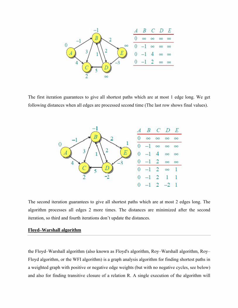
The first iteration guarantees to give all shortest paths which are at most 1 edge long. We get

following distances when all edges are processed second time (The last row shows final values).

The second iteration guarantees to give all shortest paths which are at most 2 edges long. The

algorithm processes all edges 2 more times. The distances are minimized after the second

iteration, so third and fourth iterations don’t update the distances.

Floyd–Warshall algorithm

the Floyd–Warshall algorithm (also known as Floyd's algorithm, Roy–Warshall algorithm, Roy–

Floyd algorithm, or the WFI algorithm) is a graph analysis algorithm for finding shortest paths in

a weighted graph with positive or negative edge weights (but with no negative cycles, see below)

and also for finding transitive closure of a relation R. A single execution of the algorithm will

find the lengths (summed weights) of the shortest paths between all pairs of vertices, though it

does not return details of the paths themselves.

The Floyd–Warshall algorithm was published in its currently recognized form by Robert Floyd

in 1962. However, it is essentially the same as algorithms previously published by Bernard Roy

in 1959 and also by Stephen Warshall in 1962 for finding the transitive closure of a graph.[1]

The modern formulation of Warshall's algorithm as three nested for-loops was first described by

Peter Ingerman, also in 1962.

The algorithm is an example of dynamic programming.

1 let dist be a |V| × |V| array of minimum distances initialized to ∞ (infinity)

2 for each vertex v

3 dist[v][v] ← 0

4 for each edge (u,v)

5 dist[u][v] ← w(u,v) // the weight of the edge (u,v)

6 for k from 1 to |V|

7 for i from 1 to |V|

8 for j from 1 to |V|

9 if dist[i][j] >dist[i][k] + dist[k][j]

10 dist[i][j] ← dist[i][k] + dist[k][j]

11 end if

Example

The algorithm above is executed on the graph on the left below:

Prior to the first iteration of the outer loop, labeled k=0 above, the only known paths correspond

to the single edges in the graph. At k=1, paths that go through the vertex 1 are found: in

particular, the path 2→1→3 is found, replacing the path 2→3 which has fewer edges but is

longer. At k=2, paths going through the vertices {1,2} are found. The red and blue boxes show

how the path 4→2→1→3 is assembled from the two known paths 4→2 and 2→1→3

encountered in previous iterations, with 2 in the intersection. The path 4→2→3 is not

considered, because 2→1→3 is the shortest path encountered so far from 2 to 3. At k=3, paths

going through the vertices {1,2,3} are found. Finally, at k=4, all shortest paths are found.