Embed Size (px)
Citation preview

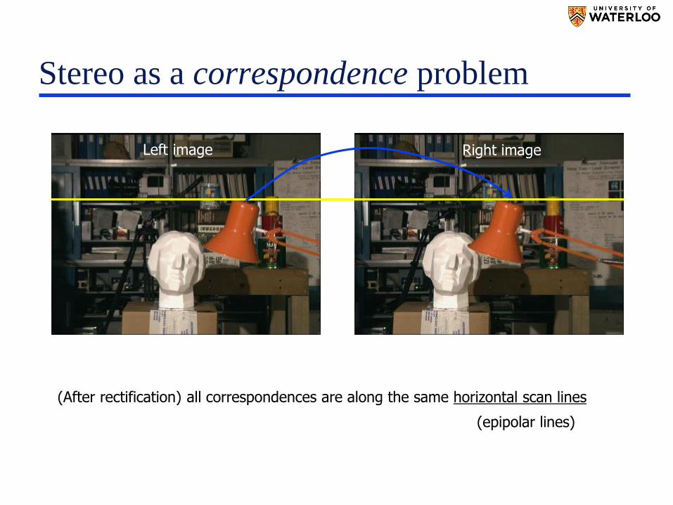
CS484/684 Computational Vision
Stereo Reconstruction
LinX computational imaging

CS484/684 Computational Vision
Stereo Reconstruction
towards dense reconstruction
• stereo is an example of dense correspondence
But, stereo is simpler since the search for correspondencesis restricted to 1D epipolar lines (versus 2D search for non-rigid motion)
• another example is dense motion estimation (optical flow)
camera rectification for stereo pairs
local stereo methods (windows)
scan-line stereo correspondenc
• optimization via DP, Viterbi, Dijkstra
global stereo
• optimization via multi-layered graph cuts
Szeliski, Chapter 11
CS484/684 Computational Vision
Stereo Reconstruction

Stereo vision
known
camera
viewpoints
Two views of the same scene from slightly different point of view
Also called, narrow baseline stereo.
Motivation: - smaller difference in views allows to find more matches (Why?)
- scene reconstruction can be formulated via simple depth map

Stereo image rectification

Stereo image rectification
Image Reprojection
• reproject image planes onto common plane parallel to line between optical centers
• homographies (3x3 transform)applied to both input images (defined by R,T ?)
• pixel motion is horizontal after this transformation• C. Loop and Z. Zhang. Computing Rectifying Homographies for Stereo
Vision. IEEE Conf. Computer Vision and Pattern Recognition, 1999.
analogous to“panning motion”

Stereo image rectification
Epipolar constraint:
T

Stereo Rectification
in this example the base line C1C2 is parallel to cube edges.
Note projective distortion.It will be much bigger
if images are taken from very different view points
(large baseline).
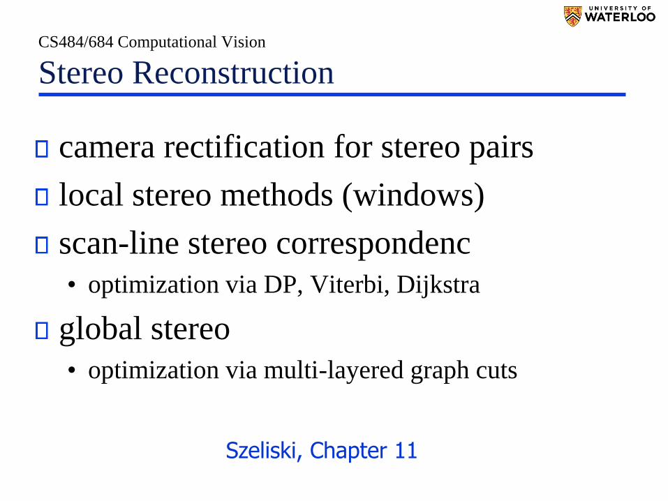
Stereo as a correspondence problem
(After rectification) all correspondences are along the same horizontal scan lines
Right imageLeft image
(epipolar lines)

C1 C2
xl xr
epipolar lines are parallel to the x axis
Rectified Cameras
xl
disparity (d)
difference between the x-coordinates of xl and xr is called the disparity
leftimage
rightimage
x
y
z
baseline

C1 C2
xl xr
Rectified Cameras
xl
disparity (d)
leftimage
rightimage
Depth = |C1C2 | · f / d
Depth
f
x
y
z
baseline

Stereo
Correspondences are described by shifts along horizontal scan lines (epipolar lines)
which can be represented by scalars (disparities)

Stereo
closer objects (smaller depths) correspond to larger disparities
Correspondences are described by shifts along horizontal scan lines (epipolar lines)
which can be represented by scalars (disparities)

Stereo
• If x-shifts (disparities) are known for all pixels in the left (or right) image then we can visualize them as a disparity map – scalar valued function d(p)
• larger disparities correspond to closer objects
Disparity map(Depth map)
Right imageLeft image
d = 0
d =15
d = 5
d =10

Stereo Correspondence problem
Human vision can solve it(even for “random dot” stereograms)
Can computer vision solve it?
Maybe
see Middlebury Stereo Databasefor the state-of-the art results
http://cat.middlebury.edu/stereo/

Stereo
Window based
• Matching rigid windows around each pixel
• Each window is matched independently
Scan-line based approach
• Finding coherent correspondences for each scan-line
• Scan-lines are independent
– DP, shortest paths
Muti-scan-line approach
• Finding coherent correspondences for all pixels
– Graph cuts

Right imageLeft image
Typical window cost function
Location with the best cost wins
C2C3
C1
f(x,y)x,y
Stereo Correspondence problem
Window based approach
Wp
p

SSD (sum of squared differences) approach
d
WpW’p-d
for any pixel p compute SSD between windows Wp and W’p-d
for all disparities d (in some interval [min_d, max_d ] )
left image (I) right image (I’)
computing SSD(p,d ) naïve implementationhas |I|*|d|*|W| operations
then

computing SSD
For each fixed d can get SSD(p,d ) at all points p
d
left image (I)
shifted right image Td(I’)
Compute the difference between the left image I and the shifted right image Td(I’)
Wp
W’p-d
Wq
W’q-d
Then, SSD(p,d) between Wp and W’p-d is equivalent to

computing SSD
For each fixed disparity d SSD(p,d )
f(x,y)x,y
left image (I)
shifted right image Td(I’)
d
Wp
Wq

computing SSD
For each fixed disparity d
Need to sum at all windows
f(x,y)x,y
left image (I)
shifted right image Td(I’)
d
Wp
Wq
SSD(p,d )

trick:
“Integral Images”
Define (integral image) fint (p) as the sum (integral)
of image f over pixels in rectangle Rp
Can compute fint (p) for all p in one pass over f (How?)
Now, for any W the sum (integral) of f inside that window
can be computed as Rbr- Rbl- Rtr+ Rtl
p
Rp
W brbl
trtl
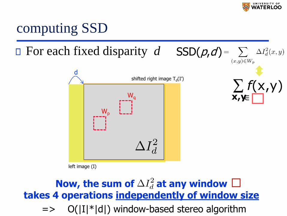
computing SSD
For each fixed disparity d
Now, the sum of at any windowtakes 4 operations independently of window size
f(x,y)x,y
=> O(|I|*|d|) window-based stereo algorithm
left image (I)
shifted right image Td(I’)
d
Wp
Wq
SSD(p,d )

Problems with Fixed Windows
small window large window
better at boundaries
noisy in low texture areas
◼ better in low texture areas
◼ blurred boundaries
Q: what do we implicitly assume when using low SSD(d,p) at a window around pixel p as a criteria for “good” disparity d ?
disparity maps for:
d = 0
d =15
d = 5
d =10

window algorithms
Maybe variable window size (pixel specific)?• What is the right window size?
• Correspondences are still found independently at each pixel (no coherence)
All window-based solutions can be though of as “local” solutions (but very fast!)
How to go to “global” solutions?
• use objectives (a.k.a. energy functions)
– regularization (e.g. spatial coherence)
• optimization
need prior knowledge to compensate
for local data ambiguity

Scan-line stereo
• Try to match coherently pixels in each scan line
• DP or shortest paths work (easy 1D optimization)
• Note: scan lines are still matched independently
– streaking artifacts
Stereo Correspondence problem
Scan-line approach

“Shortest paths” for
Scan-line stereo
Left image
Right image
q
p
e.g. Ohta&Kanade’85, Cox at.al.’96I
I
a path on this graph represents a matching function
Sleft
Sright

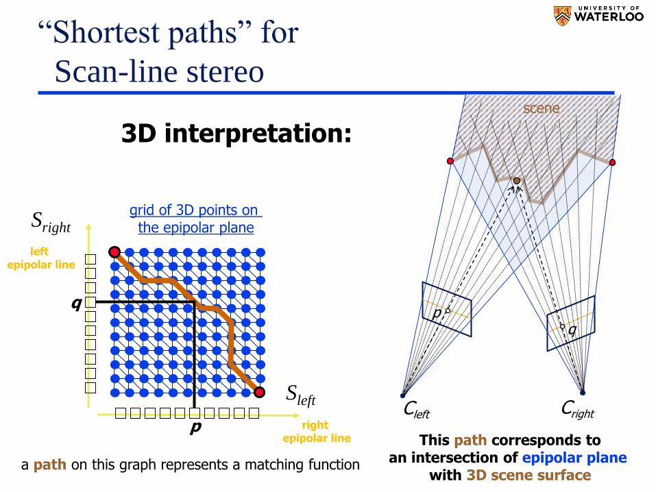
“Shortest paths” for
Scan-line stereo
q
p
3D interpretation:
right epipolar line
left epipolar line
Cleft Cright
grid of 3D points on the epipolar plane
a path on this graph represents a matching function
epipolar plane
Sleft
Sright
“Shortest paths” for
Scan-line stereo
q
p
3D interpretation:
right epipolar line
left epipolar line
Cleft Cright
grid of 3D points on the epipolar plane
qp
a path on this graph represents a matching function
This path corresponds toan intersection of epipolar plane
with 3D scene surface
Sleft
Sright
scene

“Shortest paths” for
Scan-line stereo
q
p
t
sCleft Cright
grid of 3D points on the epipolar plane
s
Sleft
Sright
3D interpretation:
t
horizontal and vertical edges on the path imply “no correspondence” (occlusion)
scene

“Shortest paths” for
Scan-line stereo
Left image
Right image
q
p
t
s
e.g. Ohta&Kanade’85, Cox at.al.’96
2)( qp II −
occlC
occlC
I
I
What is “occlusion” in general ?
Sleft
Sright
left
occ
lusi
on
rightocclusion
Edge weights:

Occlusion in stereo
right imageleft image
object
background
3D scene
cameracenters

Occlusion in stereo
right imageleft image
object
background
??
3D scene
cameracenters

Occlusion in stereo
right imageleft image
object
background
background area occluded
in the left image
backgroundarea occluded
in the right image
Note: occlusions occur at discontinuity jumps
3D scene
This right image pixel has no corresponding pixel in the left image
due to occlusionby the object
This left image pixel has no corresponding pixel in the right image
due to occlusionby the object
cameracenters

Stereo
Note: occlusions occur at discontinuity jumps
yellow marks occluded points in different viewpoints (points not visible from the central/base viewpoint).

“Shortest paths” for
Scan-line stereo
q
p
t
sCleft Cright
grid of 3D points on the epipolar plane
Sleft
Sright
3D interpretation:
horizontal and vertical edges also imply “disparity change” or “depth change”
scene
d=1
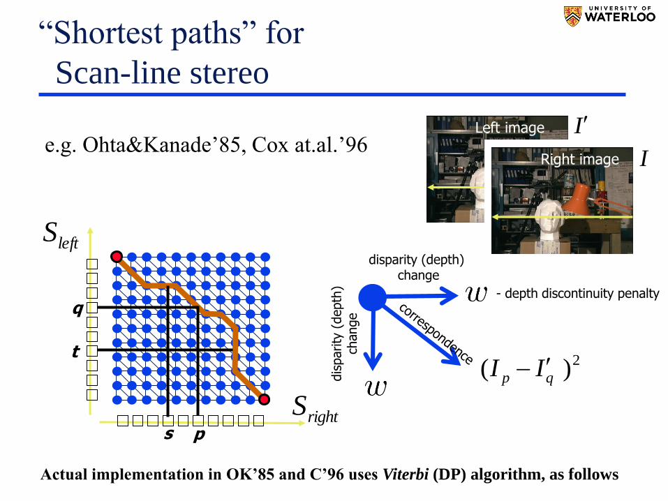
“Shortest paths” for
Scan-line stereo
Left image
Right image
Actual implementation in OK’85 and C’96 uses Viterbi (DP) algorithm, as follows
leftS
rightS
q
p
dis
parity
(depth
) ch
ange
t
disparity (depth) change
s
e.g. Ohta&Kanade’85, Cox at.al.’96
2)( qp II −
I
I
- depth discontinuity penalty

DP for scan-line stereo
Left image
Right image
rightSpleftS
2=pd
pdp
=Nqp
qp ddE},{
),(
Viterbi can handle this on non-loopy graphs
(e.g., scan-lines)
I
I
+
+=Sp
pp
Sp
pp ddVdDE ),()()( 1d
}|{ Spd p =d
rightS
Viterbi algorithm can be used to
optimize the following energy of
disparities of
pixels p on a fixed scan-line
||pdpp II
−spatial coherencephoto consistency

5-39
),( 44 nddE),( 433 ddE
)3(3E
)4(3E )4(4E
)3(4E
)2(4E
)1(4E
)4(nE
)3(nE
)2(nE
)1(nE
)2(3E
)1(3E
)4(2E
)3(2E
Dynamic Programming (DP)
Viterbi Algorithm
),(...),(),( 11322211 nnn ddEddEddE −−+++
),( 322 ddE
)1(2E
)2(2E
),( 211 ddE
Complexity: O(nm2), worst case = best case
0)1(1 =E
0)2(1 =E
0)3(1 =E
0)4(1 =E
Consider pair-wise interactions between sites (pixels) on a chain (scan-line)
states
1
2
…
m
site
s
1d 2d 3d 4d nd
)(kEp - internal “energy counters” at “site” p and “state” k
Q: how does this relate to the “shortest path” algorith (Dijkstra)?

5-40
),( 44 nddE),( 433 ddE
Dynamic Programming (DP)
Shortest paths Algorithm
),(...),(),( 11322211 nnn ddEddEddE −−+++
),( 322 ddE),( 211 ddE
Complexity: O(nm2+nm log(nm)) - worst case
Consider pair-wise interactions between sites (pixels) on a chain (scan-line)
1d 2d 3d 4d ndAlternative:
shortest pathfrom S to T
on the graph with two extra
terminals
Source
Target
E3(i,j)edge weights
E1(i,j) E2(i,j)edge weights edge weights edge weights
E4(i,j)
But, the best case could be better than Viterbi. Why?
0
0
0
0
0
0
0
0

Coherent disparity map on 2D grid?
Scan-line stereo generates streaking artifacts
Can’t use Viterbi or Dijkstra to find globally
optimal solutions on loopy graphs (e.g. grid) . • Note: there are extensions (e.g. belief propagation, TRWS)
Regularization problems in vision is an
interesting domain for optimization algorithms
Example: graph cut algorithms could find global solutions
for certain energies/losses on arbitrary (loopy) graphs.

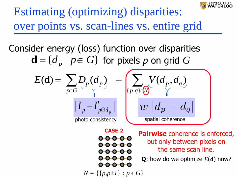
Estimating (optimizing) disparities:
over points vs. scan-lines vs. entire grid
+=Nqp
qp
Gp
pp ddVdDE},{
),()()(d
||pdpp II
−spatial coherencephoto consistency
Consider energy (loss) function over disparities
for pixels p on grid G}|{ Gpd p =d
Consider different neighborhood systems N:
N = {{p,p±1} : p ϵ G} N = {{p,q}⸦ G : |pq| ≤ 1}N = ø

Estimating (optimizing) disparities:
over points vs. scan-lines vs. entire grid
+=Nqp
qp
Gp
pp ddVdDE},{
),()()(d
||pdpp II
−spatial coherencephoto consistency
Consider energy (loss) function over disparities
for pixels p on grid G}|{ Gpd p =d
N = ø
CASE 1 smoothness term disappears
Q: how to optimize E(d) in this case?
Q: How does this relate to window-based stereo?

Estimating (optimizing) disparities:
over points vs. scan-lines vs. entire grid
+=Nqp
qp
Gp
pp ddVdDE},{
),()()(d
||pdpp II
−spatial coherencephoto consistency
Consider energy (loss) function over disparities
for pixels p on grid G}|{ Gpd p =d
N = ø
CASE 1 smoothness term disappears
Nodes/pixels do not interact (are independent).Optimization of the sum of unary terms,
e.g. , is trivial.
Estimating (optimizing) disparities:
over points vs. scan-lines vs. entire grid
+=Nqp
qp
Gp
pp ddVdDE},{
),()()(d
||pdpp II
−spatial coherencephoto consistency
Consider energy (loss) function over disparities
for pixels p on grid G}|{ Gpd p =d
N = {{p,p±1} : p ϵ G}
CASE 2Pairwise coherence is enforced,
but only between pixels on the same scan line.
Q: how do we optimize E(d) now?

Estimating (optimizing) disparities:
over points vs. scan-lines vs. entire grid
+=Nqp
qp
Gp
pp ddVdDE},{
),()()(d
||pdpp II
−spatial coherencephoto consistency
Consider energy (loss) function over disparities
for pixels p on grid G}|{ Gpd p =d
N = {{p,q}⸦ G : |pq| ≤ 1}
CASE 3
Pairwise smoothness of the disparity mapis enforced both horizontally and vertically.
NOTE: depth map coherence should be isotropic as the depth map describes 3D scene surface independent of scanline orientation.

Estimating (optimizing) disparities:
over points vs. scan-lines vs. entire grid
+=Nqp
qp
Gp
pp ddVdDE},{
),()()(d
||pdpp II
−spatial coherencephoto consistency
Consider energy (loss) function over disparities
for pixels p on grid G}|{ Gpd p =d
N = {{p,q}⸦ G : |pq| ≤ 1}
CASE 3How to optimize “pairwise” loss on loopy graphs?
NOTE 2: “Gradient descent” can find local minima for a continuous version/relaxation of E(d) where the second term becomes TV (total variation) of disparity map d.
NOTE 1: Viterbi does not apply, but its extensions (e.g. message passing) provide approximate solutions on loopy graphs.

Graph cut
for spatially coherent stereo on 2D grids
+=Nqp
qp
Gp
pp ddVdDE},{
),()()(d
||pdpp II
− || qppq ddw −spatial coherencephoto consistency
One can globally minimize the following energy of
disparities for pixels p on grid G}|{ Gpd p =d
Unlike shortest paths or Viterbi, standard s/t graph cut algorithmscan globally minimize certain types of pairwise energies on loopy graphs.

Graph cut
for spatially coherent stereo on 2D grids
+=Nqp
qp
Gp
pp ddVdDE},{
),()()(d
||pdpp II
− || qppq ddw −spatial coherencephoto consistency
pqw - weights of neighborhood edges(e.g. may be assigned
according to local intensity contrast)
One can globally minimize the following energy of
disparities for pixels p on grid G}|{ Gpd p =d

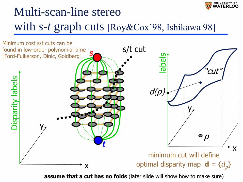
Multi-scan-line stereo
with s-t graph cuts [Roy&Cox’98, Ishikawa 98]
x
y
Multi-scan-line stereo
with s-t graph cuts [Roy&Cox’98, Ishikawa 98]
t
s s/t cut
d(p)
p
“cut”
x
y
labels
x
yDis
parity
labels
assume that a cut has no folds (later slide will show how to make sure)
Minimum cost s/t cuts can be found in low-order polynomial time [Ford-Fulkerson, Dinic, Goldberg]
minimum cut will define
optimal disparity map d = {dp}

Ishikawa&Geiger 98
What energy do we minimize this way?
Concentrate on one pair of neighboring pixels Nqp },{
p q
++= )5()2(),( qpqp DDddE
++ |3|pqw
cost of horizontal edges
cost of vertical edges
Dis
parity
labels
- 0
- 1
- 2
- 3
- 4
- 5
- 6

Ishikawa&Geiger 98
What energy do we minimize this way?
Concentrate on one pair of neighboring pixels Nqp },{
++= )()(),( qqppqp dDdDddE
+−+ || qppq ddw
cost of horizontal edges
cost of vertical edgesp q
Dis
parity
labels
- 0
- 1
- 2
- 3
- 4
- 5
- 6

Ishikawa&Geiger 98
What energy do we minimize this way?
The combined energy over the entire grid G is
=Gp
pp dDE )()(d
−+Nqp
qppq ddw},{
||
cost of horizontal edges(spatial consistency)
(photo consistency)cost of vertical edges
s
t cut

How to avoid folding?
s
t
consider three pixels },,{ rqp
p r“severed” edges are shown in red
q

S
T
How to avoid folding?
s
t
p rintroduce directed t-links
=
TqSpNpq
pqcC)(
||||
Formally, s/t cut is a partitioning of graph nodes
C={S,T} and its cost is
q
consider three pixels },,{ rqp
NOTE: this directed t-link is not “severed”
WHY?
only edges from S to T matter

S
T
How to avoid folding?
s
t
p q rSolution prohibiting folds:
add infinity cost t-links in the “up” direction
NOTE: folding cuts C = {S,T }
sever at least one of such t-linksmaking such cuts infeasible
consider three pixels },,{ rqp

S
T
How to avoid folding?
s
t
p q r
NOTE: non-folding cuts C = {S,T }
do not sever such t-links
consider three pixels },,{ rqp
Solution prohibiting folds:
add infinity cost t-links in the “up” direction

Scan-line stereo vs.
Multi-scan-line stereo
d(p)
p
“cut”
x
y
labels
labels
x
d(p)
p
Dynamic Programming(single scan line optimization)
s-t Graph Cuts(multi-scan-line optimization)

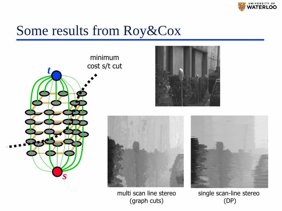
Some results from Roy&Cox
s
t
minimumcost s/t cut
multi scan line stereo(graph cuts)
single scan-line stereo (DP)
Some results from Roy&Cox
multi scan line stereo(graph cuts)
single scan-line stereo (DP)
s
t
minimumcost s/t cut

Simple Examples:
Stereo with only 2 depth layers
binary stereo
[Kolmogorov et al. CVPR 2005, IJCV 2008]
essentially,depth-based
segmentation

Simple Examples:
Stereo with only 2 depth layers
background
substitution
[Kolmogorov et al. CVPR 2005, IJCV 2008]
essentially,depth-based
segmentation

Features and
Regularizationcamera
B
. .camera A
unknown truesurface
photoconsistent3D points
photoconsistent3D points
photoconsistent3D points
photoconsistent3D points
3D volume where surface is being reconstructed(epipolar plane)
photo-consistency term
photoconsistent depth map
(epipolar lines)

Features and
Regularizationcamera
B
. .camera A
photoconsistent3D points
photoconsistent3D points
photoconsistent3D points
photoconsistent3D points
regularized depth map
3D volume where surface is being reconstructed(epipolar plane)
- regularization propagates information from textured regions (features) to ambiguous textureless regions
photo-consistency term
regularization term
- regularization helps to find smoothdepth map consistent with points uniquely matched by photoconsistency
unknown truesurface
(epipolar lines)
More features/texture always helps!

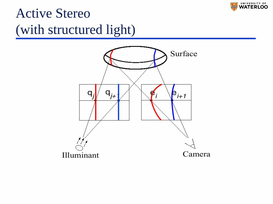
Active Stereo
(with structured light)
Project “structured” light patterns onto the object
• simplifies the correspondence problem
camera 2
camera 1
projector
camera 1
projector
Li Zhang’s one-shot stereo
Active Stereo
(with structured light)

Laser scanning
Optical triangulation
• Project a single stripe of laser light
• Scan it across the surface of the object
• This is a very precise version of structured light scanning
Digital Michelangelo Project [Levoy et al.]
http://graphics.stanford.edu/projects/mich/

Laser scanning
Digital Michelangelo Project [Levoy et al.]
http://graphics.stanford.edu/projects/mich/

Further considerations:
+=Nqp
qp
Gp
pp ddVdDE},{
),()()(d
||pdpp II
− || qppq ddw −photo-consistency
The last term is an example of convex regularization potential (loss).- easier to optimize, but- tend to over-smooth
practically preferred
robust regularization(non convex – harder to optimize)
spatial coherence
Note: once Δd is large enough,
there is no reason to keep increasing the penalty

Further considerations:
+=Nqp
qp
Gp
pp ddVdDE},{
),()()(d
||pdpp II
− || qppq ddw −photo-consistency
Similarly, robust losses are needed for photo-consistency to handle occlusions & “specularities”
practically preferred
robust regularization(non convex – harder to optimize)
spatial coherence
Note: once ΔI is large enough,
there is no reason to keep increasing the penalty/loss
?______

Further considerations:
+=Nqp
qp
Gp
pp ddVdDE},{
),()()(d
||pdpp II
−photo-consistency
Many state-of-the-art methods use higher-order regularizers
higher-order“coherence”
Q: why penalizing depth curvature instead of depth change?
dp
q r
dq dr
p
Dis
parity
valu
es
Example: curvatureneed 3 points to estimate
surface curvature
κ
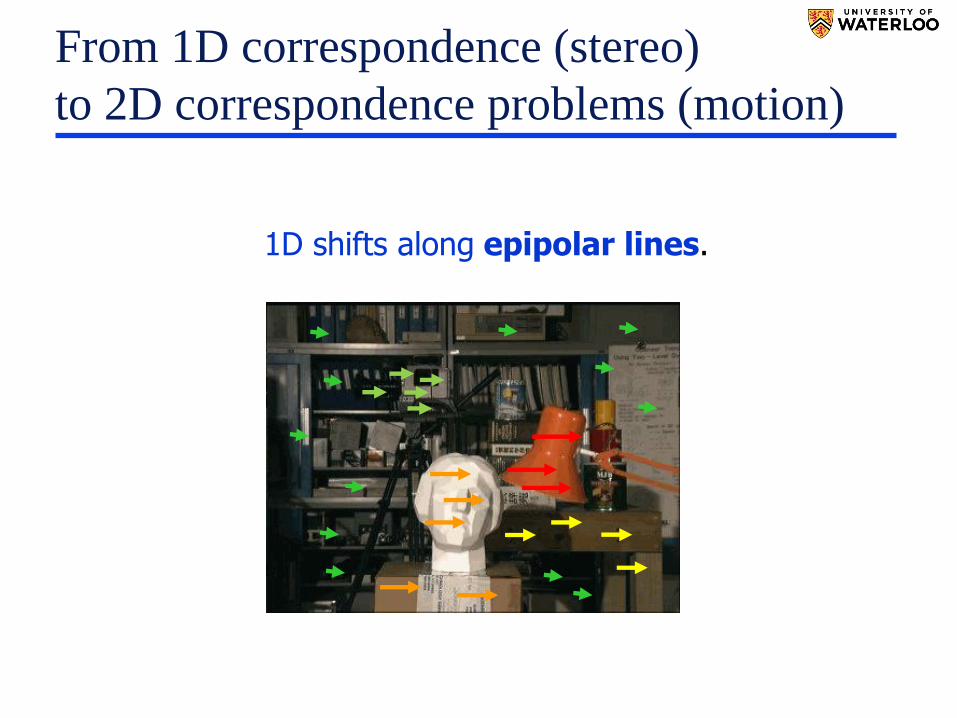
From 1D correspondence (stereo)
to 2D correspondence problems (motion)
1D shifts along epipolar lines.

From 1D correspondence (stereo)
to 2D correspondence problems (motion)
1D shifts along epipolar lines.
d = 0
d =15
d = 5
d =10
Can be represented by a scalar field (disparity map)

From 1D correspondence (stereo)
to 2D correspondence problems (motion)
In general, correspondences between two images may not be described by global models (like homography) or
by 1D shifts along epipolar lines.
For non-rigid motion the correspondences between
two video frames are described by a general optical flow

From 1D correspondence (stereo)
to 2D correspondence problems (motion)
optical flow
more difficult problem
need 2D shift vectors vp
v = {vp}
similar regularizationenergies are used for v, but harder to optimize
(e.g. Ishikawa’s method only works for scalar-valued variables)
(no epipolar line constraint)
color-consistency regularity

From 1D correspondence (stereo)
to 2D correspondence problems (motion)
optical flow
more difficult problem
need 2D shift vectors vp
v = {vp}
State-of-the-art methods segment independently moving objects
We will discuss segmentation
problemnext
(no epipolar line constraint)