Embed Size (px)
Citation preview

CS267 L11 Sources of Parallelism(2).1 Demmel Sp 1999
CS 267 Applications of Parallel Computers
Lecture 11:
Sources of Parallelism and Locality(Part 2)
James Demmel
http://www.cs.berkeley.edu/~demmel/cs267_Spr99

CS267 L11 Sources of Parallelism(2).2 Demmel Sp 1999
Recap of last lecture
° Simulation models
° A model problem: sharks and fish
° Discrete event systems
° Particle systems
° Lumped systems (Ordinary Differential Equations, ODEs)

CS267 L11 Sources of Parallelism(2).3 Demmel Sp 1999
Outline
° Continuation of (ODEs)
° Partial Differential Equations (PDEs)

CS267 L11 Sources of Parallelism(2).4 Demmel Sp 1999
Ordinary Differential EquationsODEs

CS267 L11 Sources of Parallelism(2).5 Demmel Sp 1999
Solving ODEs
° Explicit methods to compute solution(t)• Ex: Euler’s method
• Simple algorithm: sparse matrix vector multiply
• May need to take very small timesteps, especially if system is stiff (i.e. can change rapidly)
° Implicit methods to compute solution(t)• Ex: Backward Euler’s Method
• Larger timesteps, especially for stiff problems
• More difficult algorithm: solve a sparse linear system
° Computing modes of vibration• Finding eigenvalues and eigenvectors
• Ex: do resonant modes of building match earthquakes?
° All these reduce to sparse matrix problems• Explicit: sparse matrix-vector multiplication
• Implicit: solve a sparse linear system
- direct solvers (Gaussian elimination)
- iterative solvers (use sparse matrix-vector multiplication)
• Eigenvalue/vector algorithms may also be explicit or implicit
CS267 L11 Sources of Parallelism(2).6 Demmel Sp 1999
Solving ODEs - Details
° Assume ODE is x’(t) = f(x) = A*x, where A is a sparse matrix• Try to compute x(i*dt) = x[i] at i=0,1,2,…
• Approximate x’(i*dt) by (x[i+1] - x[i] )/dt
° Euler’s method:• Approximate x’(t)=A*x by (x[i+1] - x[i] )/dt = A*x[i] and solve for x[i+1]
• x[i+1] = (I+dt*A)*x[i], i.e. sparse matrix-vector multiplication
° Backward Euler’s method:• Approximate x’(t)=A*x by (x[i+1] - x[i] )/dt = A*x[i+1] and solve for x[i+1]
• (I - dt*A)*x[i+1] = x[i], i.e. we need to solve a sparse linear system of equations
° Modes of vibration• Seek solution of x’’(t) = A*x of form x(t) = sin(f*t)*x0, x0 a constant vector
• Plug in to get -f *x0 = A*x0, I.e. -f is an eigenvalue and x0 is an eigenvector of A
• Solution schemes reduce either to sparse-matrix multiplication, or solving sparse linear systems
2 2

CS267 L11 Sources of Parallelism(2).7 Demmel Sp 1999
Parallelism in Sparse Matrix-vector multiplication° y = A*x, where A is sparse and n x n
° Questions• which processors store
- y[i], x[i], and A[i,j]
• which processors compute
- y[i] = sum (from 1 to n) A[i,j] * x[j]
= (row i of A) . x … a sparse dot product
° Partitioning• Partition index set {1,…,n} = N1 u N2 u … u Np
• For all i in Nk, Processor k stores y[i], x[i], and row i of A
• For all i in Nk, Processor k computes y[i] = (row i of A) . x
- “owner computes” rule: Processor k compute the y[i]s it owns
° Goals of partitioning• balance load (how is load measured?)
• balance storage (how much does each processor store?)
• minimize communication (how much is communicated?)

CS267 L11 Sources of Parallelism(2).8 Demmel Sp 1999
Graph Partitioning and Sparse Matrices
1 1 1 1
2 1 1 1 1
3 1 1 1
4 1 1 1 1
5 1 1 1 1
6 1 1 1 1
1 2 3 4 5 6
3
6
2
1
5
4
° Relationship between matrix and graph
° A “good” partition of the graph has• equal (weighted) number of nodes in each part (load and storage balance)
• minimum number of edges crossing between (minimize communication)
° Can reorder the rows/columns of the matrix by putting all the nodes in one partition together

CS267 L11 Sources of Parallelism(2).9 Demmel Sp 1999
More on Matrix Reordering via Graph Partitioning° “Ideal” matrix structure for parallelism: (nearly) block diagonal
• p (number of processors) blocks
• few non-zeros outside these blocks, since these require communication
= *
P0
P1
P2
P3
P4

CS267 L11 Sources of Parallelism(2).10 Demmel Sp 1999
What about implicit methods and eigenproblems?° Direct methods (Gaussian elimination)
• Called LU Decomposition, because we factor A = L*U
• Future lectures will consider both dense and sparse cases
• More complicated than sparse-matrix vector multiplication
° Iterative solvers• Will discuss several of these in future
- Jacobi, Successive overrelaxiation (SOR) , Conjugate Gradients (CG), Multigrid,...
• Most have sparse-matrix-vector multiplication in kernel
° Eigenproblems• Future lectures will discuss dense and sparse cases
• Also depend on sparse-matrix-vector multiplication, direct methods
° Graph partitioning • Algorithms will be discussed in future lectures

CS267 L11 Sources of Parallelism(2).11 Demmel Sp 1999
Partial Differential Equations
PDEs

CS267 L11 Sources of Parallelism(2).12 Demmel Sp 1999
Continuous Variables, Continuous Parameters
Examples of such systems include
° Heat flow: Temperature(position, time)
° Diffusion: Concentration(position, time)
° Electrostatic or Gravitational Potential:Potential(position)
° Fluid flow: Velocity,Pressure,Density(position,time)
° Quantum mechanics: Wave-function(position,time)
° Elasticity: Stress,Strain(position,time)

CS267 L11 Sources of Parallelism(2).13 Demmel Sp 1999
Example: Deriving the Heat Equation
0 1x x+hConsider a simple problem
° A bar of uniform material, insulated except at ends
° Let u(x,t) be the temperature at position x at time t
° Heat travels from x-h to x+h at rate proportional to:
° As h 0, we get the heat equation:
d u(x,t) (u(x-h,t)-u(x,t))/h - (u(x,t)- u(x+h,t))/h
dt h
= C *
d u(x,t) d2 u(x,t)
dt dx2= C *
x-h

CS267 L11 Sources of Parallelism(2).14 Demmel Sp 1999
Explicit Solution of the Heat Equation° For simplicity, assume C=1
° Discretize both time and position
° Use finite differences with u[j,i] as the heat at• time t= i*dt (i = 0,1,2,…) and position x = j*h (j=0,1,…,N=1/h)
• initial conditions on u[j,0]
• boundary conditions on u[0,i] and u[N,i]
° At each timestep i = 0,1,2,...
° This corresponds to• matrix vector multiply (what is matrix?)
• nearest neighbors on grid
t=5
t=4
t=3
t=2
t=1
t=0u[0,0] u[1,0] u[2,0] u[3,0] u[4,0] u[5,0]
For j=0 to N
u[j,i+1]= z*u[j-1,i]+ (1-2*z)*u[j,i]+ z*u[j+1,i]
where z = dt/h2

CS267 L11 Sources of Parallelism(2).15 Demmel Sp 1999
Parallelism in Explicit Method for PDEs° Partitioning the space (x) into p largest chunks
• good load balance (assuming large number of points relative to p)
• minimized communication (only p chunks)
° Generalizes to • multiple dimensions
• arbitrary graphs (= sparse matrices)
° Problem with explicit approach• numerical instability
• solution blows up eventually if z = dt/h > .5
• need to make the timesteps very small when h is small: dt < .5*h
2
2
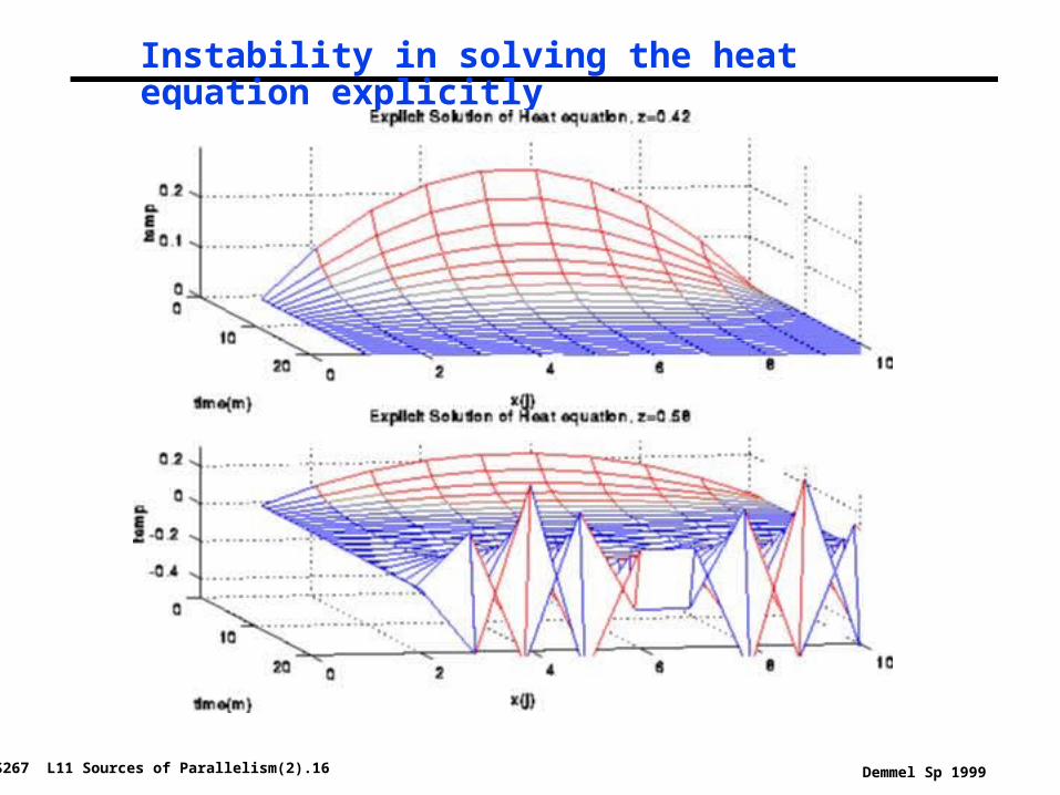
CS267 L11 Sources of Parallelism(2).16 Demmel Sp 1999
Instability in solving the heat equation explicitly

CS267 L11 Sources of Parallelism(2).17 Demmel Sp 1999
Implicit Solution° As with many (stiff) ODEs, need an implicit method
° This turns into solving the following equation
° Here I is the identity matrix and T is:
° I.e., essentially solving Poisson’s equation in 1D
(I + (z/2)*T) * u[:,i+1]= (I - (z/2)*T) *u[:,i]
2 -1
-1 2 -1
-1 2 -1
-1 2 -1
-1 2
T = 2-1 -1
Graph and “stencil”

CS267 L11 Sources of Parallelism(2).18 Demmel Sp 1999
2D Implicit Method
° Similar to the 1D case, but the matrix T is now
° Multiplying by this matrix (as in the explicit case) is simply nearest neighbor computation on 2D grid
° To solve this system, there are several techniques
4 -1 -1
-1 4 -1 -1
-1 4 -1
-1 4 -1 -1
-1 -1 4 -1 -1
-1 -1 4 -1
-1 4 -1
-1 -1 4 -1
-1 -1 4
T =
4
-1
-1
-1
-1
Graph and “stencil”

CS267 L11 Sources of Parallelism(2).19 Demmel Sp 1999
Algorithms for 2D Poisson Equation with N unknowns
Algorithm Serial PRAM Memory #Procs
° Dense LU N3 N N2 N2
° Band LU N2 N N3/2 N
° Jacobi N2 N N N
° Explicit Inv. N log N N N
° Conj.Grad. N 3/2 N 1/2 *log N N N
° RB SORN 3/2 N 1/2 N N
° Sparse LU N 3/2 N 1/2 N*log N N
° FFT N*log N log N N N
° Multigrid N log2 N N N
° Lower bound N log N N
PRAM is an idealized parallel model with zero cost communication
(see next slide for explanation)
2 22

CS267 L11 Sources of Parallelism(2).20 Demmel Sp 1999
Short explanations of algorithms on previous slide° Sorted in two orders (roughly):
• from slowest to fastest on sequential machines
• from most general (works on any matrix) to most specialized (works on matrices “like” T)
° Dense LU: Gaussian elimination; works on any N-by-N matrix
° Band LU: exploit fact that T is nonzero only on sqrt(N) diagonals nearest main diagonal, so faster
° Jacobi: essentially does matrix-vector multiply by T in inner loop of iterative algorithm
° Explicit Inverse: assume we want to solve many systems with T, so we can precompute and store inv(T) “for free”, and just multiply by it
• It’s still expensive!
° Conjugate Gradients: uses matrix-vector multiplication, like Jacobi, but exploits mathematical properies of T that Jacobi does not
° Red-Black SOR (Successive Overrelaxation): Variation of Jacobi that exploits yet different mathematical properties of T
• Used in Multigrid
° Sparse LU: Gaussian elimination exploiting particular zero structure of T
° FFT (Fast Fourier Transform): works only on matrices very like T
° Multigrid: also works on matrices like T, that come from elliptic PDEs
° Lower Bound: serial (time to print answer); parallel (time to combine N inputs)
° Details in class notes and www.cs.berkeley.edu/~demmel/ma221

CS267 L11 Sources of Parallelism(2).21 Demmel Sp 1999
Relation of Poisson’s equation to Gravity, Electrostatics° Force on particle at (x,y,z) due to particle at 0 is
-(x,y,z)/r^3, where r = sqrt(x +y +z )
° Force is also gradient of potential V = -1/r
= -(d/dx V, d/dy V, d/dz V) = -grad V
° V satisfies Poisson’s equation (try it!)
2 2 2

CS267 L11 Sources of Parallelism(2).22 Demmel Sp 1999
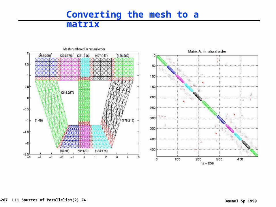
Comments on practical meshes
° Regular 1D, 2D, 3D meshes• Important as building blocks for more complicated meshes
° Practical meshes are often irregular• Composite meshes, consisting of multiple “bent” regular meshes
joined at edges
• Unstructured meshes, with arbitrary mesh points and connectivities
• Adaptive meshes, which change resolution during solution process to put computational effort where needed

CS267 L11 Sources of Parallelism(2).23 Demmel Sp 1999
Composite mesh from a mechanical structure
CS267 L11 Sources of Parallelism(2).24 Demmel Sp 1999
Converting the mesh to a matrix

CS267 L11 Sources of Parallelism(2).25 Demmel Sp 1999
Effects of Ordering Rows and Columns on Gaussian Elimination

CS267 L11 Sources of Parallelism(2).26 Demmel Sp 1999
Irregular mesh: NASA Airfoil in 2D (direct solution)

CS267 L11 Sources of Parallelism(2).27 Demmel Sp 1999
Irregular mesh: Tapered Tube (multigrid)

CS267 L11 Sources of Parallelism(2).28 Demmel Sp 1999
Adaptive Mesh Refinement (AMR)
°Adaptive mesh around an explosion°John Bell and Phil Colella at LBL (see class web page for URL)°Goal of Titanium is to make these algorithms easier to implement
in parallel

CS267 L11 Sources of Parallelism(2).29 Demmel Sp 1999
Challenges of irregular meshes (and a few solutions)° How to generate them in the first place
• Triangle, a 2D mesh partitioner by Jonathan Shewchuk
° How to partition them• ParMetis, a parallel graph partitioner
° How to design iterative solvers• PETSc, a Portable Extensible Toolkit for Scientific Computing
• Prometheus, a multigrid solver for finite element problems on irregular meshes
• Titanium, a language to implement Adaptive Mesh Refinement
° How to design direct solvers• SuperLU, parallel sparse Gaussian elimination
° These are challenges to do sequentially, the more so in parallel