CS152 Computer Architecture and Engineering CS252 Graduate

1

CS152 Computer Architecture and Engineering

CS252 Graduate Computer Architecture

Solution

VLIW, Vector, and Multithreaded Machines

Assigned 3/17/2021 Problem Set #4 Due 3/18/2021

http://inst.eecs.berkeley.edu/~cs152/sp20

The problem sets are intended to help you learn the material, and we encourage you to collaborate

with other students and to ask questions in discussion sections and office hours to understand the

problems. However, each student must turn in their own solution to the problems.

The problem sets also provide essential background material for the exam and the midterms. The

problem sets will be graded primarily on an effort basis, but if you do not work through the problem

sets you are unlikely to succeed on the exam or midterms! We will distribute solutions to the

problem sets on the day the problem sets are due to give you feedback. Homework assignments

are due at the beginning of class on the due date, and all assignments are to be submitted through

Gradescope. Late homework will not be accepted, except for extreme circumstances and with

prior arrangement.

2

Problem 1: Trace Scheduling

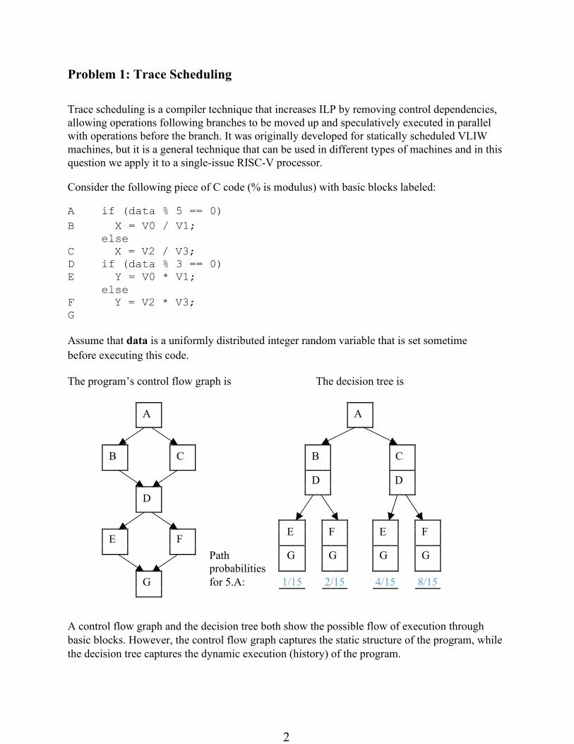
Trace scheduling is a compiler technique that increases ILP by removing control dependencies,

allowing operations following branches to be moved up and speculatively executed in parallel

with operations before the branch. It was originally developed for statically scheduled VLIW

machines, but it is a general technique that can be used in different types of machines and in this

question we apply it to a single-issue RISC-V processor. Consider the following piece of C code (% is modulus) with basic blocks labeled: A if (data % 5 == 0) B X = V0 / V1;

else

C X = V2 / V3; D if (data % 3 == 0)

E Y = V0 * V1;

else F Y = V2 * V3;

G

Assume that data is a uniformly distributed integer random variable that is set sometime

before executing this code.

The program’s control flow graph is The decision tree is

A A

B C B C

D D

D

E F E F E

F

Path G G G G

probabilities

G

for 5.A: 1/15 2/15 4/15 8/15

A control flow graph and the decision tree both show the possible flow of execution through

basic blocks. However, the control flow graph captures the static structure of the program, while

the decision tree captures the dynamic execution (history) of the program.

3

Problem 1.A

On the decision tree, label each path with the probability of traversing that path. For example,

the leftmost block will be labeled with the total probability of executing the path ABDEG.

(Hint: you might want to write out the cases). Circle the path that is most likely to be executed.

Circle: ACDFG

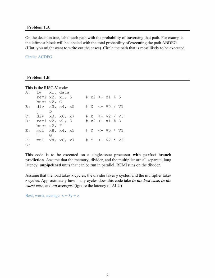
Problem 1.B

This is the RISC-V code: A: lw x1, data

remi x2, x1, 5 # x2 <- x1 % 5

bnez x2, C

B: div x3, x4, x5 # X <- V0 / V1

j D

C: div x3, x6, x7 # X <- V2 / V3

D: remi x2, x1, 3 # x2 <- x1 % 3

bnez x2, F

E: mul x8, x4, x5 # Y <- V0 * V1

j G

F: mul x8, x6, x7 # Y <- V2 * V3

G:

This code is to be executed on a single-issue processor with perfect branch

prediction. Assume that the memory, divider, and the multiplier are all separate, long

latency, unpipelined units that can be run in parallel. REMI runs on the divider.

Assume that the load takes x cycles, the divider takes y cycles, and the multiplier takes

z cycles. Approximately how many cycles does this code take in the best case, in the

worst case, and on average? (ignore the latency of ALU)

Best, worst, average: x + 3y + z

4

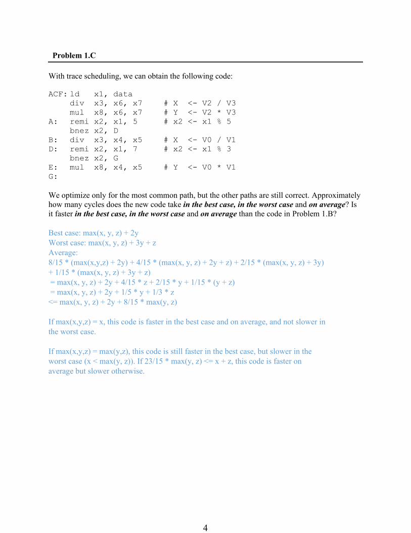
Problem 1.C

With trace scheduling, we can obtain the following code:

ACF: ld x1, data

div x3, x6, x7 # X <- V2 / V3

mul x8, x6, x7 # Y <- V2 * V3

A: remi x2, x1, 5 # x2 <- x1 % 5

bnez x2, D

B: div x3, x4, x5 # X <- V0 / V1

D: remi x2, x1, 7 # x2 <- x1 % 3

bnez x2, G

E: mul x8, x4, x5 # Y <- V0 * V1

G:

We optimize only for the most common path, but the other paths are still correct. Approximately

how many cycles does the new code take in the best case, in the worst case and on average? Is

it faster in the best case, in the worst case and on average than the code in Problem 1.B?

Best case: max(x, y, z) + 2y

Worst case: max(x, y, z) + 3y + z

Average:

8/15 * (max(x,y,z) + 2y) + 4/15 * (max(x, y, z) + 2y + z) + 2/15 * (max(x, y, z) + 3y)

+ 1/15 * (max(x, y, z) + 3y + z)

= max(x, y, z) + 2y + 4/15 * z + 2/15 * y + 1/15 * (y + z)

= max(x, y, z) + 2y + 1/5 * y + 1/3 * z

<= max(x, y, z) + 2y + 8/15 * max(y, z)

If max(x,y,z) = x, this code is faster in the best case and on average, and not slower in

the worst case.

If max(x,y,z) = max(y,z), this code is still faster in the best case, but slower in the

worst case (x < max(y, z)). If 23/15 * max(y, z) <= x + z, this code is faster on

average but slower otherwise.

5

Problem 2: VLIW machines

In this problem, we consider the execution of a code segment on a VLIW processor. The code

we consider is the SAXPY kernel, which scales a vector X by a constant A, adding this quantity

to a vector Y.

for(i = 0; i < N; i++) {

Y[i] = Y[i] + A*X[i];

}

loop: 1. ld f1, 0(x1) # f1 = X[i]

2. fmul f2, f0, f1 # A * X[i]

3. ld f3, 0(x2) # f3 = Y[i]

4. fadd f4, f2, f3 # f4 = Y[i] + A*X[i]

5. sd f4, 0(x2) # Y[i] = f4

6. addi x1, x1, 4 # bump pointer


8. bne x1, x3, loop # loop

Now we have a VLIW machine with seven execution units:

- two ALU units, latency one cycle, also used for branch operations

- three memory units, latency three cycles, fully pipelined, each unit can perform either a store

or a load - two FPU units, latency four cycles, fully pipelined, one unit can perform fadd operations,

the other fmul operations.

Below is the format of a VLIW instruction:

Int Op 1 Int Op 2 Mem Op 1 Mem Op 2 Mem Op 3 FP Add FP Mul

Our machine has no interlocks. The result of an operation is written to the register file immediately

after it has gone through the corresponding execution unit: one cycle after issue for ALU

operations, three cycles for memory operations and four cycles for FPU operations. The old values

can be read from the registers until they have been overwritten.

When writing code for this machine, you may assume:

1) The arrays are long (> 32 elements)

2) The arrays have an even number of elements

6

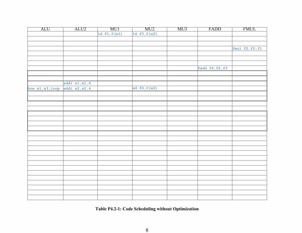
Problem 2.A: No Code Optimization

Schedule instructions for the VLIW machine in Table P4.2-1 without loop unrolling and

software pipelining . What is the throughput of the loop in the code in floating point operations

per cycle (FLOPS/cycle)?

Throughput = 2 / 12 = 1/6 FLOPS/cycle

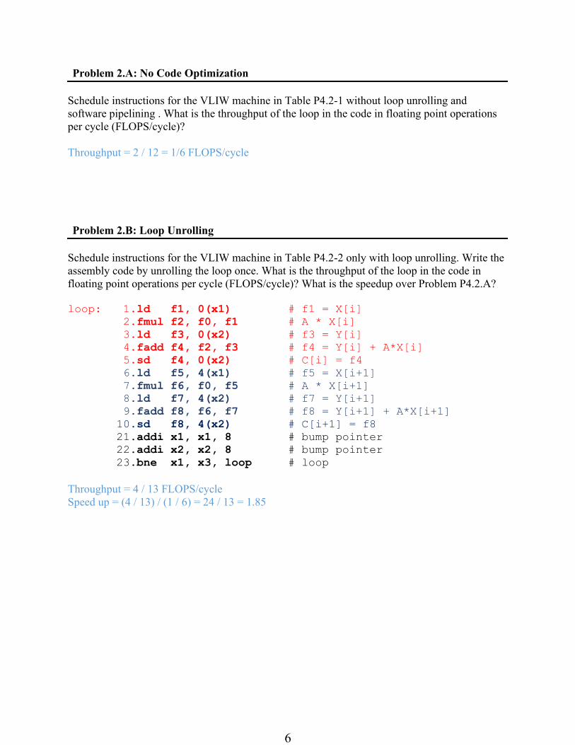
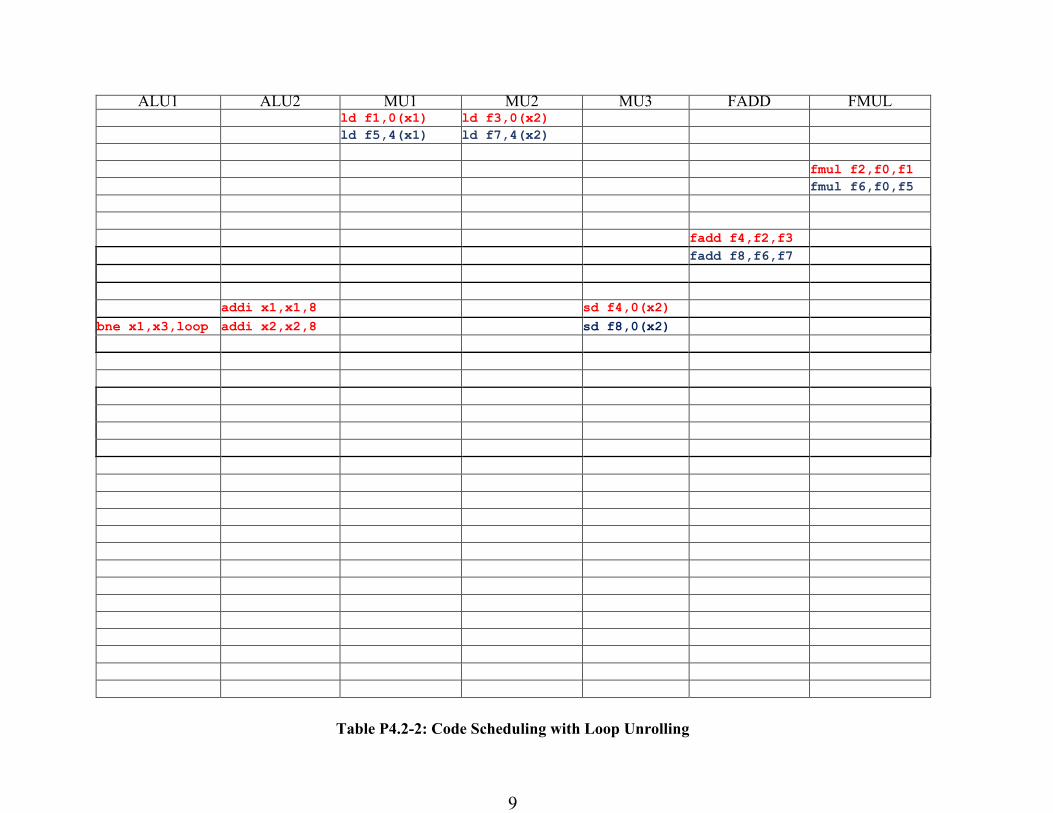
Problem 2.B: Loop Unrolling

Schedule instructions for the VLIW machine in Table P4.2-2 only with loop unrolling. Write the

assembly code by unrolling the loop once. What is the throughput of the loop in the code in

floating point operations per cycle (FLOPS/cycle)? What is the speedup over Problem P4.2.A?

loop: 1. ld f1, 0(x1) # f1 = X[i]

2. fmul f2, f0, f1 # A * X[i]

3. ld f3, 0(x2) # f3 = Y[i]

4. fadd f4, f2, f3 # f4 = Y[i] + A*X[i]

5. sd f4, 0(x2) # C[i] = f4

6. ld f5, 4(x1) # f5 = X[i+1]

7. fmul f6, f0, f5 # A * X[i+1]

8. ld f7, 4(x2) # f7 = Y[i+1]

9. fadd f8, f6, f7 # f8 = Y[i+1] + A*X[i+1]

10. sd f8, 4(x2) # C[i+1] = f8



23. bne x1, x3, loop # loop

Throughput = 4 / 13 FLOPS/cycle

Speed up = (4 / 13) / (1 / 6) = 24 / 13 = 1.85

7

Problem 2.C: Software Pipelining

Schedule instructions for the VLIW machine in Table P4.2-3 only with software pipelining.

Include the prologue and the epilogue in Table P4.2-3. What is the throughput of the loop in the

code in floating point operations per cycle (FLOPS/cycle)? What is the speedup over Problem

P4.2.A?

Throughput = 2 / 2 = 1 FLOPS

Speed up = (1 / 1) / (1/ 6) = 6

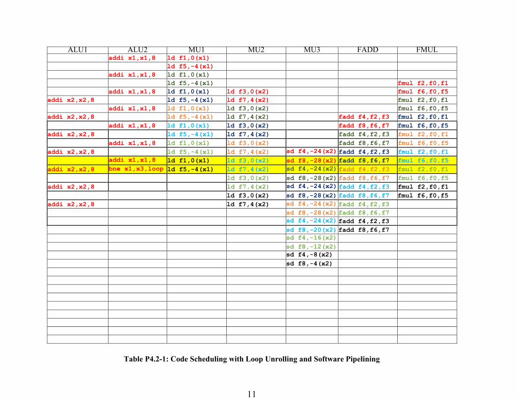
Problem 2.D: Loop Unrolling + Software Pipelining

Schedule instructions for the VLIW machine in Table P4.2-4 with both loop unrolling and

software pipelining. Unroll the loop once as in Problem 2.B. Include the prologue and the

epilogue in Table P4.2-3. What is the throughput of the loop in the code in floating point

operations per cycle (FLOPS/cycle)? What is the speedup over Problem 2.A?

Throughput = 4 / 2 FLOPS

Speed up = (4 / 2) / (1 / 6) = 12

8

ALU ALU2 MU1 MU2 MU3 FADD FMUL ld f1,0(x1) ld f3,0(x2)

fmul f2,f0,f1

fadd f4,f2,f3

addi x1,x1,4

bne x1,x3,loop addi x2,x2,4 sd f4,0(x2)

Table P4.2-1: Code Scheduling without Optimization

9

ALU1 ALU2 MU1 MU2 MU3 FADD FMUL ld f1,0(x1) ld f3,0(x2)

ld f5,4(x1) ld f7,4(x2)

fmul f2,f0,f1

fmul f6,f0,f5

fadd f4,f2,f3

fadd f8,f6,f7

addi x1,x1,8 sd f4,0(x2)

bne x1,x3,loop addi x2,x2,8 sd f8,0(x2)

Table P4.2-2: Code Scheduling with Loop Unrolling

10

ALU1 ALU2 MU1 MU2 MU3 FADD FMUL addi x1,x1,4 ld f1,0(x1)

addi x1,x1,4 ld f1,0(x1)

fmul f2,f0,f1

addi x2,x2,4 addi x1,x1,4 ld f1,0(x1) ld f3,0(x2)

fmul f2,f0,f1


fadd f4,f2,f3 fmul f2,f0,f1


fadd f4,f2,f3 fmul f2,f0,f1


bne x1,x3,loop sd f4,-16(x2) fadd f4,f2,f3 fmul f2,f0,f1


sd f4,-16(x2) fadd f4,f2,f3 fmul f2,f0,f1


sd f4,-16(x2) fadd f4,f2,f3


sd f4,-8(x2)

sd f4,-4(x2)

Table P4.2-3: Code Scheduling with Software Pipelining

11

ALU1 ALU2 MU1 MU2 MU3 FADD FMUL addi x1,x1,8 ld f1,0(x1)

ld f5,-4(x1)


ld f5,-4(x1) fmul f2,f0,f1

addi x1,x1,8 ld f1,0(x1) ld f3,0(x2) fmul f6,f0,f5

addi x2,x2,8 ld f5,-4(x1) ld f7,4(x2) fmul f2,f0,f1

addi x1,x1,8 ld f1,0(x1) ld f3,0(x2) fmul f6,f0,f5

addi x2,x2,8 ld f5,-4(x1) ld f7,4(x2) fadd f4,f2,f3 fmul f2,f0,f1

addi x1,x1,8 ld f1,0(x1) ld f3,0(x2) fadd f8,f6,f7 fmul f6,f0,f5

addi x2,x2,8 ld f5,-4(x1) ld f7,4(x2) fadd f4,f2,f3 fmul f2,f0,f1

addi x1,x1,8 ld f1,0(x1) ld f3,0(x2) fadd f8,f6,f7 fmul f6,f0,f5

addi x2,x2,8 ld f5,-4(x1) ld f7,4(x2) sd f4,-24(x2) fadd f4,f2,f3 fmul f2,f0,f1

addi x1,x1,8 ld f1,0(x1) ld f3,0(x2) sd f8,-28(x2) fadd f8,f6,f7 fmul f6,f0,f5

addi x2,x2,8 bne x1,x3,loop ld f5,-4(x1) ld f7,4(x2) sd f4,-24(x2) fadd f4,f2,f3 fmul f2,f0,f1

ld f3,0(x2) sd f8,-28(x2) fadd f8,f6,f7 fmul f6,f0,f5

addi x2,x2,8 ld f7,4(x2) sd f4,-24(x2) fadd f4,f2,f3 fmul f2,f0,f1

ld f3,0(x2) sd f8,-28(x2) fadd f8,f6,f7 fmul f6,f0,f5

addi x2,x2,8 ld f7,4(x2) sd f4,-24(x2) fadd f4,f2,f3




sd f4,-16(x2)

sd f8,-12(x2)

sd f4,-8(x2)

sd f8,-4(x2)

Table P4.2-1: Code Scheduling with Loop Unrolling and Software Pipelining

12

Problem 3: Vector Machines

In this problem, we analyze the performance of vector machines. We start with a baseline vector

processor with the following features:

• 32 elements per vector register

• 8 lanes

• One ALU per lane: 1 cycle latency

• One load/store unit per lane: 4 cycle latency, fully pipelined

• No dead time

• No support for chaining

• Scalar instructions execute on a separate 5-stage pipeline

To simplify the analysis, we assume a magic memory system with no bank conflicts and no

cache misses. We consider execution of the following loop:

C code for (i = 0; i < N; i++) {

C[i] = A[i] + B[i] – 1; }

loop: 1. LV V1, (x1) # load A

2. LV V2, (x2) # load B

3. ADDV V3, V1, V2 # A + B

4. SUBVS V4, V3, x4 # subtract x4 = 1

5. SV V4, (x3) # store C

6. ADDI x1, x1, 128 # bump pointer



9. SUBI x5, x5, 32 # i++ (x5 = N)

10. BNQZ x5, loop # loop

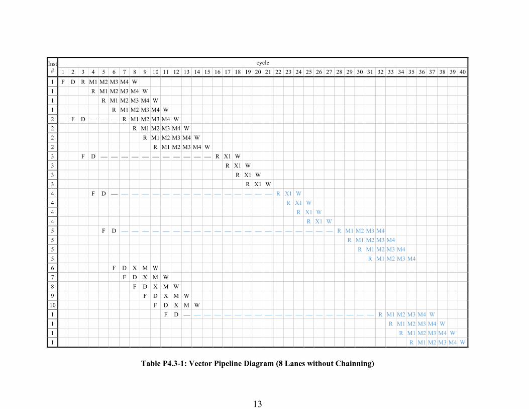
Problem 3.A: Simple Vector Processor

Complete the pipeline diagram in Table P4.4-1 of the baseline vector processor running

the given code. The following supplementary information explains the diagram: Scalar instructions execute in 5 cycles: fetch (F), decode (D), execute (X), memory (M),

and writeback (W). A vector instruction is also fetched (F) and decoded (D). Then, it stalls

(—) until its required vector functional unit is available. With no chaining, a dependent

vector instruction stalls until the previous instruction finishes writing back all of its

elements. A vector instruction is pipelined across all the lanes in parallel. For each element,

the operands are read (R) from the vector register file, the operation executes on the

load/store unit (M) or the ALU (X), and the result is written back (W) to the vector register

file. A stalled vector instruction does not block a scalar instruction from executing.

13

Inst

#

cycle

1 2 3 4 5 6 7 8 9 10 11 12 13 14 15 16 17 18 19 20 21 22 23 24 25 26 27 28 29 30 31 32 33 34 35 36 37 38 39 40

1 F D R M1 M2 M3 M4 W

1 R M1 M2 M3 M4 W

1 R M1 M2 M3 M4 W

1 R M1 M2 M3 M4 W

2 F D ⎯ ⎯ ⎯ R M1 M2 M3 M4 W

2 R M1 M2 M3 M4 W

2 R M1 M2 M3 M4 W

2 R M1 M2 M3 M4 W

3 F D ⎯ ⎯ ⎯ ⎯ ⎯ ⎯ ⎯ ⎯ ⎯ ⎯ ⎯ R X1 W

3 R X1 W

3 R X1 W

3 R X1 W

4 F D ⎯ ⎯ ⎯ ⎯ ⎯ ⎯ ⎯ ⎯ ⎯ ⎯ ⎯ ⎯ ⎯ ⎯ ⎯ ⎯ R X1 W

4 R X1 W

4 R X1 W

4 R X1 W

5 F D ⎯ ⎯ ⎯ ⎯ ⎯ ⎯ ⎯ ⎯ ⎯ ⎯ ⎯ ⎯ ⎯ ⎯ ⎯ ⎯ ⎯ ⎯ ⎯ ⎯ ⎯ R M1 M2 M3 M4

5 R M1 M2 M3 M4

5 R M1 M2 M3 M4

5 R M1 M2 M3 M4

6 F D X M W

7 F D X M W

8 F D X M W

9 F D X M W

10 F D X M W

1 F D ⎯ ⎯ ⎯ ⎯ ⎯ ⎯ ⎯ ⎯ ⎯ ⎯ ⎯ ⎯ ⎯ ⎯ ⎯ ⎯ ⎯ ⎯ ⎯ R M1 M2 M3 M4 W

1 R M1 M2 M3 M4 W

1 R M1 M2 M3 M4 W

1 R M1 M2 M3 M4 W

Table P4.3-1: Vector Pipeline Diagram (8 Lanes without Chainning)

14

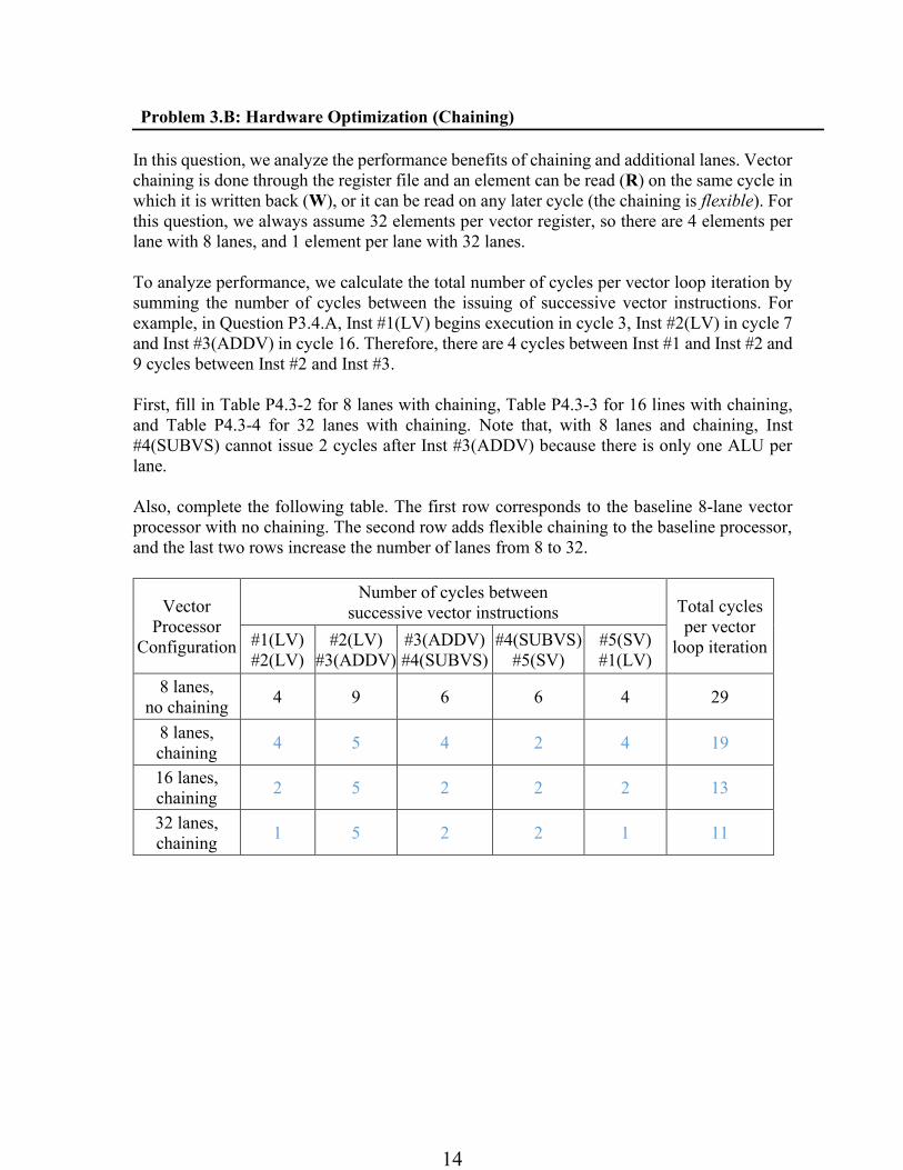
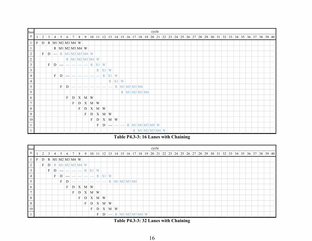
Problem 3.B: Hardware Optimization (Chaining)

In this question, we analyze the performance benefits of chaining and additional lanes. Vector

chaining is done through the register file and an element can be read (R) on the same cycle in

which it is written back (W), or it can be read on any later cycle (the chaining is flexible). For

this question, we always assume 32 elements per vector register, so there are 4 elements per

lane with 8 lanes, and 1 element per lane with 32 lanes.

To analyze performance, we calculate the total number of cycles per vector loop iteration by

summing the number of cycles between the issuing of successive vector instructions. For

example, in Question P3.4.A, Inst #1(LV) begins execution in cycle 3, Inst #2(LV) in cycle 7

and Inst #3(ADDV) in cycle 16. Therefore, there are 4 cycles between Inst #1 and Inst #2 and

9 cycles between Inst #2 and Inst #3.

First, fill in Table P4.3-2 for 8 lanes with chaining, Table P4.3-3 for 16 lines with chaining,

and Table P4.3-4 for 32 lanes with chaining. Note that, with 8 lanes and chaining, Inst

#4(SUBVS) cannot issue 2 cycles after Inst #3(ADDV) because there is only one ALU per

lane.

Also, complete the following table. The first row corresponds to the baseline 8-lane vector

processor with no chaining. The second row adds flexible chaining to the baseline processor,

and the last two rows increase the number of lanes from 8 to 32.

Vector

Processor

Configuration

Number of cycles between

successive vector instructions Total cycles

per vector

loop iteration #1(LV)

#2(LV)

#2(LV)

#3(ADDV)

#3(ADDV)

#4(SUBVS)

#4(SUBVS)

#5(SV)

#5(SV)

#1(LV)

8 lanes,

no chaining 4 9 6 6 4 29

8 lanes,

chaining 4 5 4 2 4 19

16 lanes,

chaining 2 5 2 2 2 13

32 lanes,

chaining 1 5 2 2 1 11

15

Inst

#

cycle

1 2 3 4 5 6 7 8 9 10 11 12 13 14 15 16 17 18 19 20 21 22 23 24 25 26 27 28 29 30 31 32 33 34 35 36 37 38 39 40

1 F D R M1 M2 M3 M4 W

1 R M1 M2 M3 M4 W

1 R M1 M2 M3 M4 W

1 R M1 M2 M3 M4 W

2 F D ⎯ ⎯ ⎯ R M1 M2 M3 M4 W

2 R M1 M2 M3 M4 W

2 R M1 M2 M3 M4 W

2 R M1 M2 M3 M4 W

3 F D ⎯ ⎯ ⎯ ⎯ ⎯ ⎯ ⎯ R X1 W

3 R X1 W

3 R X1 W

3 R X1 W

4 F D ⎯ ⎯ ⎯ ⎯ ⎯ ⎯ ⎯ ⎯ ⎯ ⎯ R X1 W

4 R X1 W

4 R X1 W

4 R X1 W

5 F D ⎯ ⎯ ⎯ ⎯ ⎯ ⎯ ⎯ ⎯ ⎯ ⎯ ⎯ R M1 M2 M3 M4

5 R M1 M2 M3 M4

5 R M1 M2 M3 M4

5 R M1 M2 M3 M4

6 F D X M W

7 F D X M W

8 F D X M W

9 F D X M W

10 F D X M W

1 F D ⎯ ⎯ ⎯ ⎯ ⎯ ⎯ ⎯ ⎯ ⎯ R M1 M2 M3 M4 W

1 R M1 M2 M3 M4 W

1 R M1 M2 M3 M4 W

1 R M1 M2 M3 M4 W

Table P4.3-2: 8 Lanes with Chaining

16

Inst

#

cycle

1 2 3 4 5 6 7 8 9 10 11 12 13 14 15 16 17 18 19 20 21 22 23 24 25 26 27 28 29 30 31 32 33 34 35 36 37 38 39 40

1 F D R M1 M2 M3 M4 W

1 R M1 M2 M3 M4 W

2 F D ⎯ R M1 M2 M3 M4 W

2 R M1 M2 M3 M4 W

3 F D ⎯ ⎯ ⎯ ⎯ ⎯ R X1 W

3 R X1 W

4 F D ⎯ ⎯ ⎯ ⎯ ⎯ ⎯ R X1 W

4 R X1 W

5 F D ⎯ ⎯ ⎯ ⎯ ⎯ ⎯ ⎯ R M1 M2 M3 M4

5 R M1 M2 M3 M4

6 F D X M W

7 F D X M W

8 F D X M W

9 F D X M W

10 F D X M W

1 F D ⎯ ⎯ ⎯ R M1 M2 M3 M4 W

1 R M1 M2 M3 M4 W


Inst

#

cycle

1 2 3 4 5 6 7 8 9 10 11 12 13 14 15 16 17 18 19 20 21 22 23 24 25 26 27 28 29 30 31 32 33 34 35 36 37 38 39 40

1 F D R M1 M2 M3 M4 W

2 F D R M1 M2 M3 M4 W

3 F D ⎯ ⎯ ⎯ ⎯ R X1 W

4 F D ⎯ ⎯ ⎯ ⎯ ⎯ R X1 W

5 F D ⎯ ⎯ ⎯ ⎯ ⎯ ⎯ R M1 M2 M3 M4

6 F D X M W

7 F D X M W

8 F D X M W

9 F D X M W

10 F D X M W

1 F D ⎯ R M1 M2 M3 M4 W


17

Problem 4: Multithreading

This problem evaluates the effectiveness of multithreading using a simple database benchmark.

The benchmark searches for an entry in a linked list built from the following structure, which

contains a key, a pointer to the next node in the linked list, and a pointer to the data entry.

struct node { int

key; struct node *next;

struct data *ptr; }

The following RISC-V code shows the core of the benchmark, which traverses the linked list

and finds an entry with a particular key. loop: LW x3, 0(x1) # load a key

LW x4, 4(x1) # load the next pointer

SEQ x3, x3, x2 # set x3 if x3 == x2

BNEZ x3, end # found the entry

ADD x1, x0, x4

BNEZ x4, loop # check the next node

end: We run this benchmark on a single-issue in-order processor. The processor can fetch and issue

(dispatch) one instruction per cycle. If an instruction cannot be issued due to a data dependency,

the processor stalls. Integer instructions take one cycle to execute and the result can be used in

the next cycle. For example, if SEQ is executed in cycle 1, BNEZ can be executed in cycle 2.

We also assume that the processor has a perfect branch predictor with no penalty for both taken

and not-taken branches. Problem 4.A

Assume that our system does not have a cache. Each memory operation directly accesses main

memory and takes 100 CPU cycles. The load/store unit is fully pipelined, and non-blocking.

After the processor issues a memory operation, it can continue executing instructions until it

reaches an instruction that is dependent on an outstanding memory operation. How many cycles

does it take to execute one iteration of the loop in steady state? 104 cycles

Instruction Start Cycle End Cycle LW x3, 0(x1) 0 100 LW x4, 4(x1) 1 101 SEQ x3, x3, x2 101 101 BNEZ x3, End 102 102 ADD x1, x0, x4 103 103 BNEZ x1, Loop 104 104

18

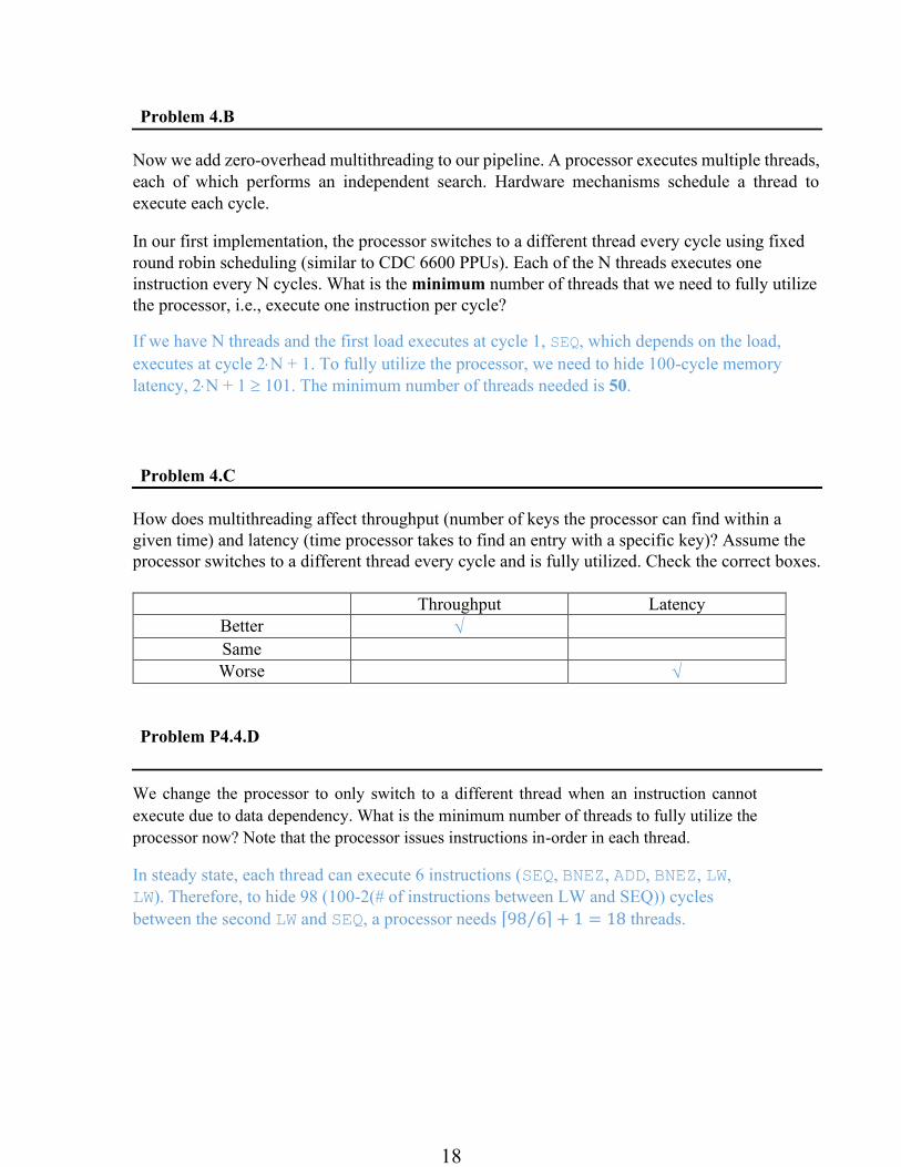
Problem 4.B

Now we add zero-overhead multithreading to our pipeline. A processor executes multiple threads,

each of which performs an independent search. Hardware mechanisms schedule a thread to

execute each cycle. In our first implementation, the processor switches to a different thread every cycle using fixed

round robin scheduling (similar to CDC 6600 PPUs). Each of the N threads executes one

instruction every N cycles. What is the minimum number of threads that we need to fully utilize

the processor, i.e., execute one instruction per cycle? If we have N threads and the first load executes at cycle 1, SEQ, which depends on the load,

executes at cycle 2N + 1. To fully utilize the processor, we need to hide 100-cycle memory

latency, 2N + 1 101. The minimum number of threads needed is 50.

Problem 4.C

How does multithreading affect throughput (number of keys the processor can find within a

given time) and latency (time processor takes to find an entry with a specific key)? Assume the

processor switches to a different thread every cycle and is fully utilized. Check the correct boxes.

Throughput Latency

Better

Same

Worse

Problem P4.4.D

We change the processor to only switch to a different thread when an instruction cannot

execute due to data dependency. What is the minimum number of threads to fully utilize the

processor now? Note that the processor issues instructions in-order in each thread. In steady state, each thread can execute 6 instructions (SEQ, BNEZ, ADD, BNEZ, LW,

LW). Therefore, to hide 98 (100-2(# of instructions between LW and SEQ)) cycles

between the second LW and SEQ, a processor needs ⌈98 6⁄ ⌉ + 1 = 18 threads.

19

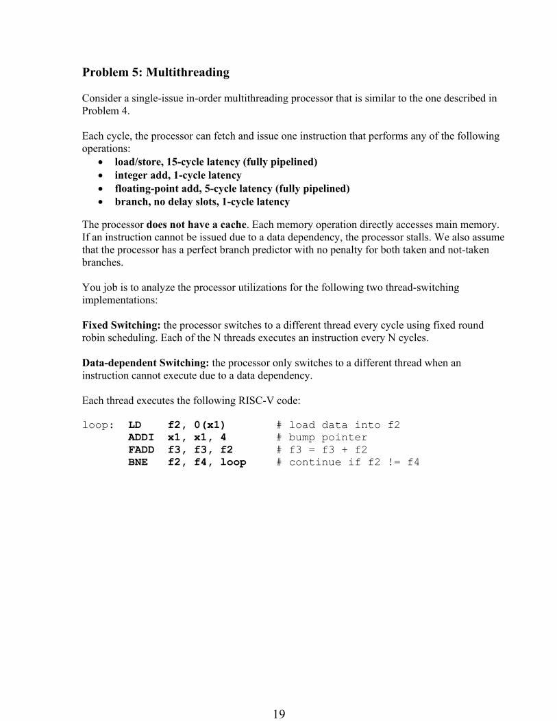
Problem 5: Multithreading

Consider a single-issue in-order multithreading processor that is similar to the one described in

Problem 4.

Each cycle, the processor can fetch and issue one instruction that performs any of the following

operations:

• load/store, 15-cycle latency (fully pipelined)

• integer add, 1-cycle latency

• floating-point add, 5-cycle latency (fully pipelined)

• branch, no delay slots, 1-cycle latency The processor does not have a cache. Each memory operation directly accesses main memory.

If an instruction cannot be issued due to a data dependency, the processor stalls. We also assume

that the processor has a perfect branch predictor with no penalty for both taken and not-taken

branches.

You job is to analyze the processor utilizations for the following two thread-switching

implementations:

Fixed Switching: the processor switches to a different thread every cycle using fixed round

robin scheduling. Each of the N threads executes an instruction every N cycles.

Data-dependent Switching: the processor only switches to a different thread when an

instruction cannot execute due to a data dependency.

Each thread executes the following RISC-V code:

loop: LD f2, 0(x1) # load data into f2

ADDI x1, x1, 4 # bump pointer

FADD f3, f3, f2 # f3 = f3 + f2

BNE f2, f4, loop # continue if f2 != f4

20

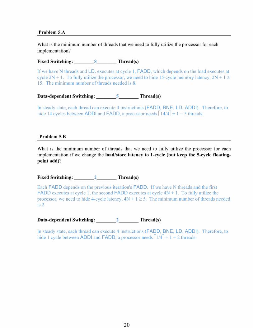
Problem 5.A

What is the minimum number of threads that we need to fully utilize the processor for each

implementation? Fixed Switching: ________8________ Thread(s) If we have N threads and LD. executes at cycle 1, FADD, which depends on the load executes at

cycle 2N + 1. To fully utilize the processor, we need to hide 15-cycle memory latency, 2N + 1

15. The minimum number of threads needed is 8.

Data-dependent Switching: ________5________ Thread(s)

In steady state, each thread can execute 4 instructions (FADD, BNE, LD, ADDI). Therefore, to

hide 14 cycles between ADDI and FADD, a processor needs 14/4 + 1 = 5 threads.

Problem 5.B

What is the minimum number of threads that we need to fully utilize the processor for each

implementation if we change the load/store latency to 1-cycle (but keep the 5-cycle floating-

point add)?

Fixed Switching: ________2________ Thread(s) Each FADD depends on the previous iteration's FADD. If we have N threads and the first

FADD executes at cycle 1, the second FADD executes at cycle 4N + 1. To fully utilize the

processor, we need to hide 4-cycle latency, 4N + 1 5. The minimum number of threads needed

is 2. Data-dependent Switching: ________2________ Thread(s)

In steady state, each thread can execute 4 instructions (FADD, BNE, LD, ADDI). Therefore, to

hide 1 cycle between ADDI and FADD, a processor needs 1/4 + 1 = 2 threads.

21

Problem 5.C

Consider a Simultaneous Multithreading (SMT) machine with limited hardware resources.

Circle the following hardware constraints that can limit the total number of threads that the

machine can support. For the item(s) that you circle, briefly describe the minimum requirement

to support N threads.

(A) Number of Functional Unit:

Since not all the treads are executed each cycle, the number of functional units is not a constraint

that limits the total number of threads that the machine can support.

(B) Number of Physical Registers:

We need at least [N (number of architecture registers)] physical registers for an in-order

system. Since it is SMT, it is actually least [N (number of architecture registers) + 1] physical

registers, because you can’t free a physical register until the next instruction commits to that

same architectural register.

(C) Data Cache Size:

This is for performance reasons.

(D) Data Cache Associatively:

This is for performance reasons.

Documents

CS152 Computer Architecture and Engineering CS252 Graduate