CS 600.226: Data Structuresphf/2016/fall/cs226/... · balanced search trees: • AVL trees guarantee worst case O(log n) operations by carefully accounting for the tree height •

CS 600.226: Data Structures Michael Schatz Nov 7, 2016 Lecture 28: HashTables

Remember: javac –Xlint:all & checkstyle *.java & JUnit Solutions should be independently written!

Assignment 8: Due Thursday Nov 10 @ 10pm

Part 1: AVL Trees

Binary Search Tree

<k

A BST is a binary tree with a special ordering property: If a node has value k, then the left child (and its descendants) will have values smaller than k; and the right child (and its descendants) will have

values greater than k

>k

k

Tree Rotations

>A >B

B

>A <B

<A <B

A

<A <B

A

>A <B

>A >B

B

Note: Rotating a BST maintains the BST condition!

Green < A < Brown < B < Purple

right-rotation(B)

left-rotation(A)

Complete Example Insert these values: 4 5 7 2 1 3

4 4 \ 5

4 \ 5 \ 7

5 / \4 7

5 / \ 4 7 /2 5 / \ 4 7 / 2 /1

5 / \ 2 7 / \ 1 4

5 / \ 2 7 / \ 1 4 / 3

5 / \ 4 7 / 2 / \ 1 3

4 / \ 2 5 / \ \ 1 3 7

ins(5)

ins(7)

ins(2)

ins(1) ins(3)

l(4)

r(4)

l(2) r(5)

Note: AVL Violations are fixed bottom up

Removing

Remove leaf

is easy

6 / \ 3 8 / \ / \1 4 7 9

6 / \ 3 8 / \ \1 4 9

6 / \ 3 9 / \ 1 4

7 8 6

Remove with only one child Is easy

Remove Internal Node:

Swap with predecessor /successor

4 / \ 3 9 / 1

9 / 3 / \ 1 4

or

Remove from AVL just like removing from regular BST: Find successor Swap with that element, Remove the node that you just swapped.

Make sure to update the height fields, and rebalance if necessary

Implementation Notes

•  Rotations can be applied in constant time! •  Inserting a node into an AVL tree requires O(lg n) time and

guarantees O(lg(n)) height

•  Track the height of each node as a separate field •  The alternative is to track when the tree is lopsided, but just as

hard and more error prone •  Don’t recompute the heights from scratch, it is easy to compute

but requires O(n) time! •  Since we are guaranteeing the tree will have height lg(n), just use

an integer •  Only update the affected nodes

Check out Appendix B for some very useful tips on hacking AVL trees!

AVL Tree Balance By construction, an AVL tree can never become “too unbalanced” •  AVL condition ensures left and right children differ by at most 1 •  But they arent necessarily “full”

n=1 n=2 n=3 n=4 n=5

n=6 n=7

Sparse AVL Trees How many nodes are in the sparsest AVL tree of height h •  Sparse means fewest nodes with height h •  Does it still include an exponential number of nodes?

S1

h=1 n=1

S2

h=2 n=2

S3

h=3 n=4

S4

h=4 n=7

S5

h=5 n=12

Sparse AVL Trees How many nodes are in the sparsest AVL tree of height h •  Sparse means fewest nodes with height h •  Does it still include an exponential number of nodes?

S1

h=1 n=1

S1 = 1

S2

h=2 n=2

S2 = 2

S3

h=3 n=4

S3 = S2 + S1 + 1

S4

h=4 n=7

S4 = S3 + S2 + 1

S5

h=5 n=12

S5 = S4 + S3 + 1

Sh = Sh-1 + Sh-2 + 1

Fibonacci Sequence

f(1) f(0)

f(2) f(1) f(1) f(0) f(1) f(0) f(1) f(0)

f(4) f(3) f(3) f(2)

f(3) f(2) f(2) f(1) f(2) f(1) f(1) f(0)

F(6)

f(5) f(4)

public static int fib(int n) { if (n <= 1) { return 1; } return fib(n-1) + fib(n-2); }

Nodes in an AVL Tree How many nodes are in the sparsest AVL tree of height h •  Sparse means fewest nodes with height h •  Does it still include an exponential number of nodes?

S(h) = F(h + 3) − 1

Fibonacci grows exponentially at φn

AVL Trees grow exponentially at φn-1

Therefore the height of any AVL tree is O(lg n)

Part 2: Treaps

BSTs versus Heaps

<k >k

k

≥p ≥p

p

≤p

BST

All keys in left subtree of k are < k, all keys in right are >k Tricky to balance, but fast to find

Heap

All children of the node with priority p have priority ≥p Easy to balance, but hard to find (except min/max)

BSTs versus Heaps

<k >k

k

≥p ≥p

p

≤p

BST

All keys in left subtree of k are < k, all keys in right are >k Tricky to balance, but fast to find

Heap

All children of the node with priority p have priority ≥p Easy to balance, but hard to find (except min/max)

Treap

<k/p

>k/p

k/p

A treap is a binary search tree where the nodes have both user specified keys (k) and internally assigned priorities (p). When inserting, use standard BST insertion algorithm, but then use rotations to iteratively move up the node while it has lower priority than its parent (analogous to a heap, but with rotations)

Treap Reflections

Insert the following pairs: 7/3, 2/0, 1/7, 8/2, 3/9, 5/1, 4/7

Insert the following pairs: 7/1, 2/2, 1/3, 8/4, 3/5, 5/6, 4/7 7/1 / \ 2/2 8/4 / \1/3 3/5 \ 5/6 / 4/7

2/0 / \1/7 5/1 / \ 4/7 8/2 / / 3/9 7/3

Since the priorities are in sorted order, becomes a standard BST and may have O(n) height

With a standard BST, for 2 to be root it would have to be the first key inserted, and 5 would have to proceed all

the other keys except 1, …

It is as if we saw the sequence: 2,5,8,7,1,4,3

Note priorities in sorted order: 2/0, 5/1, 8/2/, 7/3, 1/7, 4/7, 3/9

What priorities should we assign to maintain a balanced tree?

Math.random()

Using random priorities essentially shuffles the input data (which might have bad linear height)

into a random permutation

that we expect to have O(log n) height J

It is possible that we could randomly shuffle into a poor tree configuration, but that is extremely rare.

In most practical applications, a treap will perform just fine, and will often outperform an AVL tree that guarantees O(log n) height but has higher

constants

Random Tree Height

## Trying all permutations of 14 distinct keys numtrees: 87,178,291,200 average height: 6.63 maxheights[0]: 0 0.00% maxheights[1]: 0 0.00% maxheights[2]: 0 0.00% maxheights[3]: 0 0.00% maxheights[4]: 21964800 0.03% maxheights[5]: 10049994240 11.53% maxheights[6]: 33305510656 38.20% maxheights[7]: 27624399104 31.69% maxheights[8]: 12037674752 13.81% maxheights[9]: 3393895680 3.89% maxheights[10]: 652050944 0.75% maxheights[11]: 85170176 0.10% maxheights[12]: 7258112 0.01% maxheights[13]: 364544 0.00% maxheights[14]: 8192 0.00%

Random Tree Height ## Trying all permutations of 15 distinct keys $ tail -f heights.15.log tree[838452000000]: 10 1 11 8 15 14 5 3 6 9 4 12 13 2 7 maxheight: 6 tree[838453000000]: 10 1 11 9 5 7 13 2 8 6 12 14 15 3 4 maxheight: 7 tree[838454000000]: 10 1 11 9 5 2 3 8 13 12 14 4 7 6 15 maxheight: 7 tree[838455000000]: 10 1 11 9 5 13 8 15 4 12 3 2 6 14 7 maxheight: 7 tree[838456000000]: 10 1 11 9 5 15 6 13 12 3 4 14 7 2 8 maxheight: 7 tree[838457000000]: 10 1 11 9 6 8 13 3 15 2 14 7 5 12 4 maxheight: 7 tree[838458000000]: 10 1 11 9 6 3 5 2 7 8 4 12 13 14 15 maxheight: 7 tree[838459000000]: 10 1 11 9 6 14 4 8 13 15 12 5 2 3 7 maxheight: 7 tree[838460000000]: 10 1 11 9 7 6 15 5 4 14 2 13 3 12 8 maxheight: 9 tree[838461000000]: 10 1 11 9 7 4 13 5 12 14 3 6 8 2 15 maxheight: 7 tree[838462000000]: 10 1 11 9 7 12 3 5 15 13 6 14 4 8 2 maxheight: 7 tree[838463000000]: 10 1 11 9 7 15 4 2 3 12 14 13 5 8 6 maxheight: 7 tree[838464000000]: 10 1 11 9 8 5 7 6 14 12 3 2 13 4 15 maxheight: 7 tree[838465000000]: 10 1 11 9 8 2 13 15 6 3 12 14 5 4 7 maxheight: 9 tree[838466000000]: 10 1 11 9 8 13 3 6 5 2 14 4 7 12 15 maxheight: 8 tree[838467000000]: 10 1 11 9 4 6 5 12 7 2 3 8 13 14 15 maxheight: 7 …

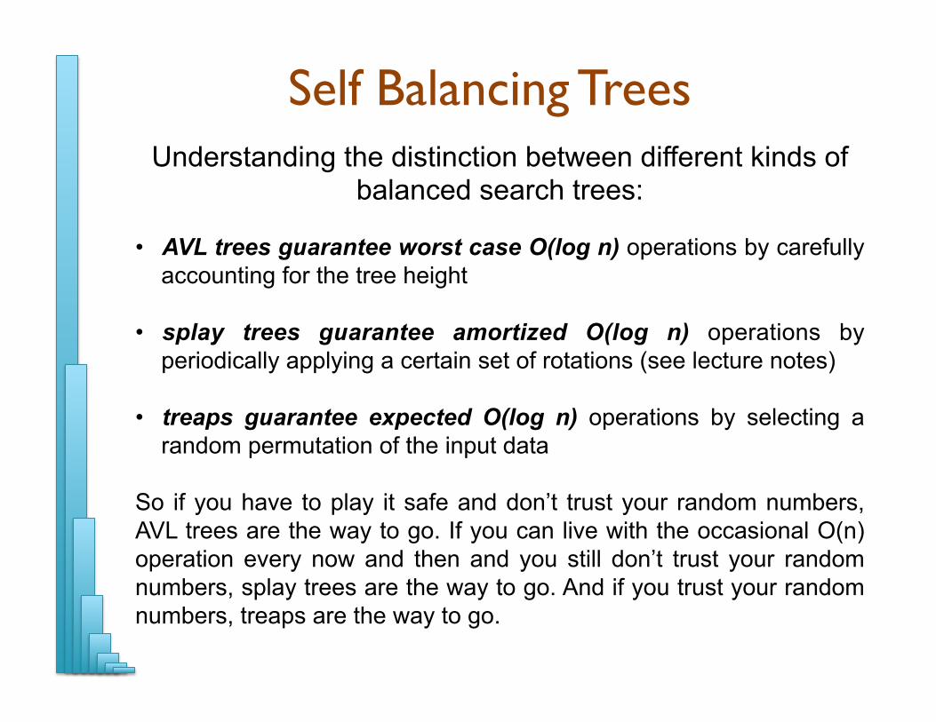
Self Balancing Trees Understanding the distinction between different kinds of

balanced search trees:

•  AVL trees guarantee worst case O(log n) operations by carefully accounting for the tree height

•  splay trees guarantee amortized O(log n) operations by periodically applying a certain set of rotations (see lecture notes)

•  treaps guarantee expected O(log n) operations by selecting a random permutation of the input data

So if you have to play it safe and don’t trust your random numbers, AVL trees are the way to go. If you can live with the occasional O(n) operation every now and then and you still don’t trust your random numbers, splay trees are the way to go. And if you trust your random numbers, treaps are the way to go.

Part 3: Hash Tables

Maps aka dictionaries

aka associative arrays

Mike -> Malone 323Peter -> Malone 223Joanne -> Malone 225Zack -> Malone 160 suiteDebbie -> Malone 160 suiteYair -> Malone 160 suiteRon -> Garland 242

Key (of Type K) -> Value (of Type V)

Note you can have multiple keys with the same value, But not okay to have one key map to more than 1 value

Maps, Sets, and Arrays

Mike -> TruePeter -> TrueJoanne -> TrueZack -> TrueDebbie -> TrueYair -> TrueRon -> True

Sets as Map<T, Boolean>

0 -> Mike1 -> Peter2 -> Joanne3 -> Zack4 -> Debbie5 -> Yair6 -> Ron

Array as Map<Integer, T>

Maps are extremely flexible and powerful, and therefore are extremely widely used

Built into many common languages: Awk, Python, Perl, JavaScript…

Could we do everything in O(lg n) time or faster? => Balanced Search Trees

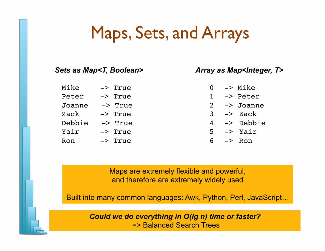
Maps, Sets, and Arrays

Mike -> TruePeter -> TrueJoanne -> TrueZack -> TrueDebbie -> TrueYair -> TrueRon -> True

Sets as Map<T, Boolean>

0 -> Mike1 -> Peter2 -> Joanne3 -> Zack4 -> Debbie5 -> Yair6 -> Ron

Array as Map<Integer, T>

Maps are extremely flexible and powerful, and therefore are extremely widely used

Built into many common languages: Awk, Python, Perl, JavaScript…

Could we do everything in O(lg n) time or faster? => Balanced Search Trees

ADT: Arrays

0 1 2 … n-1 n-2 n-3

t t t … t t t

get(2

)

put(n

-2, X

)

a:

•  Fixed length data structure •  Constant time get() and put() methods •  Definitely needs to be generic J

Hashing

Hash Function enables: Map<K, V> -> Map<Integer, V> -> Array<V> •  h(): K -> Integer for any possible key K •  h() should distribute the keys uniformly over all integers •  if k1 and k2 are “close”, h(k1) and h(k2) should be “far” apart

Typically want to return a small integer, so that we can use it as an index into an array •  An array with 4B cells in not very practical if we only expect a few thousand

to a few million entries •  How do we restrict an arbitrary integer x into a value up to some maximum

value n? 0 <= x % n < n

Compression function: c(i) = abs(i) % length(a) Transforms from a large range of integers to a small range (to store in array a)

Array[“Mike”] = 10; Array[“Peter”] = 15 BST:O(lg n) -> Hash:O(1)

Array[13] = 10; Array[42] = 15 O(1)

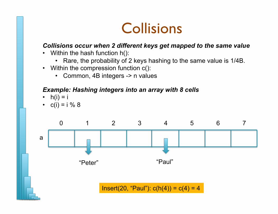
Collisions Collisions occur when 2 different keys get mapped to the same value •  Within the hash function h():

•  Rare, the probability of 2 keys hashing to the same value is 1/4B. •  Within the compression function c():

•  Common, 4B integers -> n values

a

0 1 2 3 4 5 6 7

Example: Hashing integers into an array with 8 cells •  h(i) = i •  c(i) = i % 8

insert(1, “Peter”): c(h(1)) = c(1) = 1

“Peter”

a

0 1 2 3 4 5 6 7


Insert(20, “Paul”): c(h(4)) = c(4) = 4

“Peter” “Paul”




a

0 1 2 3 4 5 6 7


insert(15, “Mary”): c(h(15)) = c(15) = 7

“Peter” “Paul” “Mary”




a

0 1 2 3 4 5 6 7


get(15): get(c(h(15))) = get(c(15)) = get(7) => “Mary”





J

a

0 1 2 3 4 5 6 7


has(4): has(c(h(4)) = has(c(4)) = has(4) => “Paul”





L

a

0 1 2 3 4 5 6 7


insert(4, “Beverly”): c(h(4)) = c(4) = 4

“Peter” “Paul” “Mary” “Beverly”




L

a

0 1 2 3 4 5 6 7


Two problems caused by collisions: False positives: How do we know the key is the one we want? Collision Resolution: What do we do when 2 keys map to same location?





a

0 1 2 3 4 5 6 7


Two problems caused by collisions: False positives: How do we know the key is the one we want? Collision Resolution: What do we do when 2 keys map to same location?

(1,“Peter”) (20, “Paul”) (15, “Mary”)




Separate chaining

a

0 1 2 3 4 5 6 7

Use Array<List<V>> instead of an Array<V> to store the entries

(1,“Peter”) (20, “Paul”) (15, “Mary”)

o o o


Separate chaining

a

0 1 2 3 4 5 6 7


(1,“Peter”) (20, “Paul”) (15, “Mary”)

o o


(4, “Beverly”)

o

Separate chaining

a

0 1 2 3 4 5 6 7


(1,“Peter”) (20, “Paul”) (15, “Mary”)

o o

Using separate chaining we could implement the Map<K,V> interface J

(4, “Beverly”)

o

Seems fast, but how fast do we expect it to be?

Separate Chaining Analysis Assume the table has just 1 cell:

All n items will be in a linked list => O(n) insert/find/remove L

Assume table has m cells AND h() evenly distributes the keys •  Every cell is equally likely to be selected to store key k, so the n items

should be evenly distributed across m slots •  Average number of items per slot: n/m

•  Also called the load factor (commonly written as α) •  Also the probability of a collision when inserting a new key

•  Empty table: 0/m probability •  After 1st item: 1/m •  After 2nd item: 2/m

Assume the hash function h() always returns a constant value All n items will be in a linked list => O(n) insert/find/remove L

Expected time for unsuccessful search:

Expected time for successful search:

O(1+n/m)

O(1+n/m/2) => O(1+n/m)

If n < c*m, then we can expect constant time! J

Next Steps 1.  Reflect on the magic and power of Hash Tables! 2.  Assignment 8 due Thursday November 10 @ 10pm

Welcome to CS 600.226 http://www.cs.jhu.edu/~cs226/

Questions?

Documents

CS 600.226: Data Structuresphf/2016/fall/cs226/... · balanced search trees: • AVL trees guarantee worst case O(log n) operations by carefully accounting for the tree height •