CS 372: Computational Geometry Lecture 9 Point Location

CS 372: Computational GeometryLecture 9

Point Location

Antoine Vigneron

King Abdullah University of Science and Technology

December 11, 2012

Antoine Vigneron (KAUST) CS 372 Lecture 9 December 11, 2012 1 / 39

1 Introduction

2 Randomized incremental construction of a trapezoidal map

3 Analysis

4 Point location data structure

5 Conclusion


Outline

A geometric data structure problem: Point location.

Solved using:

Trapezoidal map.

Randomized Incremental Construction (RIC)

Reference:

Textbook Chapter 6.

Dave Mount’s lecture notes, lectures 14 and 15.


http://0-www.springerlink.com.library.kaust.edu.sa/content/k18243

http://www.cs.umd.edu/~mount/754

Problem Statement

Problem (Point location in a planar subdivision)

Preprocess a planar straight-line graph G so as to be able to answer thefollowing queries efficiently:

Input: A query point q.

Output: The face of G that contains q.

Remarks:

One dimension Two dimensions

Sorting Trapezoidal map

Searching Point location

Quicksort RIC

Random BST History graph


Results

Expected query time: O(log n)

Expected preprocessing time: O(n log n)

Expected space usage: O(n)

Can we hope to do better?I There is a deterministic algorithm with same time and space bounds.


Trapezoidal Map

Start with a PSLG G.I General position assumption: No two vertices have same x-coordinate.

The trapezoidal map T (G) is obtained by drawing vertical edgesdownward and upward from each vertex.

G T (G)

We draw a bounding box around G so that there is no infinite face,hence each faces of T (G) is a trapezoid.


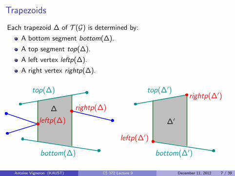
Trapezoids

Each trapezoid ∆ of T (G) is determined by:

A bottom segment bottom(∆).

A top segment top(∆).

A left vertex leftp(∆).

A right vertex rightp(∆).

∆ rightp(∆)

top(∆)

bottom(∆)

leftp(∆) ∆′

top(∆′)

bottom(∆′)

rightp(∆′)

leftp(∆′)


Neighbors

Definition (neighbors)

We say that two trapezoids are neighbors if they share a vertical edge.

By our general position assumption, a trapezoid has at most 4neighbors.


Data Structure

Doubly Connected Edge List,

or simpler: Just store adjacency relations from previous two slides.I The vertices of G are represented by their coordinates.I The edges of G point to their left and right endpoints.I Each trapezoid ∆ of T (G) has pointers to:

F bottom(∆), top(∆).F leftp(∆), rightp(∆).F Its (at most) 4 neighbors.


Trapezoidal Map

The trapezoidal map T (G) has:

O(n) vertices,

O(n) edges,

O(n) faces (=trapezoids).

Point location in a trapezoidal map:

Construct the trapezoidal map by RIC.

Use the history graph to perform point location.


Point Location in a PSLG G

First compute T (G) and associated search structure by RIC.

Then augment the search structure with pointers from each face ofT (G) to the face in G that contains it.

Perform point location in T (G).

Find the corresponding face in G.


Randomized Incremental Construction of T (G )

Let S denote the set of edges of G.

Compute a random permutation (s1, s2, . . . sn) of S .

We denote Si = {s1, s2 . . . si} for any i 6 n.

Initialize the data structure: DCEL or adjacency relations for thebounding box.

Initialize a conflict list for the left endpoints of the segments of S .I Initially, only one conflict list (for the interior face of the bounding box)

that gathers all the segments in S .I Keep a pointer from each s ∈ S to its conflicting trapezoid, which is

the interior face of the bounding box.


Conflict Lists: Example

s3

∆′

s6

s2

s8

s5

s7

s4

s1

∆

∆′′

L(∆) = {s5, s8}L(∆′) = {s6}L(∆′′) = {s7}


Idea

At step i we maintain:

A representation of T (Si ).

For each trapezoid ∆ of T (Si ):I a conflict list L(∆) of pointers to all the segments in S \ Si whose left

endpoint is in ∆.

For each s ∈ S \ Si :I a pointer to the trapezoid ∆ of T (Si ) that contains its left endpoint.

Then we insert si+1 and update this data structure.


Inserting si

si

si may cross several trapezoids of T (Si−1).


Inserting si

si

Each trapezoid is split into at most 4 trapezoids.


Inserting si

si

Some trapezoids are merged.


Terminology

Definition

We say that a trapezoid ∆ of T (Si ) is defined by a segment s ∈ Si if ∆does not appear in T (Si \ {s}).

∆

top(∆)

bottom(∆)

sHere, the trapezoid ∆ is defined onlyby the three segments top(∆),bottom(∆) and s.

Observation

A trapezoid is defined by at most 4 segments.


Zone of si

The zone of si in T (Si−1) is the union of all the cells that intersect si .

si

It is the union of all the trapezoids of T (Si−1) that are destroyed when weinsert si .


Zone of si

It is also the union of all the trapezoids in T (Si ) that are defined by si .

si

It is the union of all the trapezoids created when we insert si .


Updating the Trapezoidal Map

From our data structure, we know which trapezoid in T (Si−1)contains the left endpoint of si .

We proceed from left to right and update the trapezoidal map.

Everything is done within the zone of si .

We sweep from left to right.

Only two trapezoids intersect the sweep line at any time.

Let ki be the number of trapezoids in T (Si ) that are defined by si .

There are at most ki events.

So the update can be done in O(ki ) time.


Updating the Conflict Information

We also need to update the conflict lists.

Non-inserted left endpoints move from destroyed trapezoids to newlycreated trapezoids.

Each destroyed trapezoid is contained in the union of 4 newtrapezoids.

So update can be done in time O(Xi ) where Xi is the number of leftendpoints of non-inserted segments in the zone of si .

Xi is also the number of left endpoints in the trapezoids of T (Si ) thatare defined by si .


Analysis: Bound on E [ki ]

Trapezoid ∆ ∈ T (Si ) is newly created iff it is defined by si .

For each segment s ∈ Si and for each trapezoid ∆ ∈ T (Si ), letI δ(∆, s) = 1 if s defines ∆.I δ(∆, s) = 0 otherwise.

The number of trapezoids defined by s is∑∆∈T (Si )

δ(∆, s).



We use backward analysis.

We assume that Si is fixed.

Then si can be any segment in Si with probability 1/i .

Then

E [ki ] =1

i

∑s∈Si

∑∆∈T (Si )

δ(∆, s)

.

We reverse the order of summation:

E [ki ] =1

i

∑∆∈T (Si )

∑s∈Si

δ(∆, s)

I Note: This technique is called double counting.



What is∑

s∈Si δ(∆, s)?

It is the number of segments that define ∆.

So it is at most 4.

Therefore

E [ki ] 61

i

∑∆∈T (Si )

4.

There are O(i) trapezoids in T (Si ) so

E [ki ] =1

iO(i) = O(1).


Analysis: Bound on Xi

We also need to bound the number Xi of non-inserted left endpointsin newly created trapezoids.

Backward analysis: Si is fixed.

Let s ∈ S \ Si .

Let ∆ be the trapezoid in T (Si ) that contains the left endpoint of s.

What is the probability that ∆ is newly created?I It is the probability that si is one of the (at most 4) segments that

define ∆.I So it is at most 4/i .

So

E [Xi ] 64(n − i)

i.


Analysis

Let T (n) be the construction time.

Then by linearity of expectation

E [T (n)] = O

(n∑

i=1

E [ki ] + E [Xi ]

).

So

E [T (n)] = O

(n∑

i=1

1 +n

i

)= O

(n

n∑i=1

1

i

)= O(n log n).

It is an expected time on worst case input.


Point Location Data Structure

Reference: D. Mount lecture 15.

The history graph records the history of the RIC.

Lecture 7:I Quicksort ⇒ history graph ⇒ searching.

Here:I RIC ⇒ history graph ⇒ point location.

In Lecture 7, the history graph was a tree.I Here it is a DAG: Directed Acyclic Graph.

Expected preprocessing time: O(n log n).

Expected space usage: O(n).

Expected query time: O(log n).


Example (1)

s1

A

B

A′

B ′

A

Trapezoidal map

B B ′ A′

History graph

(The root correspondsto the bounding box)


Example (2)

s1

A

B

A

Trapezoidal map History graph

s2

B ′

A′ B ′ A′

A′ and B ′ are deleted fromthe trapezoidal map butremain in the history graph

B


Update of the History Graph

Connect each destroyed trapezoid to all the newly created trapezoidsthat overlap it.

Overlap means the interiors intersect; not just touching along an edge.


Example (3)

s1

A

B

C D E G

A B

DC F E G

B ′ A′

s2

F

The history graph is not a tree: Two edges point to F .

It is a DAG.


Example (4)

s1

A

B

G

D E

C

s3

A B A′B ′

DC EF G

s2F


Example (5)

s1

A

B

s3

I

J

K

M

N

H

A A′B ′B

FC D E G

H I J L K M Ns2

L

F


Analysis

Update time of DAG:

In time proportional to the number of new trapezoids.I That is, O(ki ).

We have seen that E [ki ] = O(1).

Hence, building the DAG takes O(n) time overall.

We also have to count O(n log n) time for the RIC.


Answering Queries

The query point q is given by its coordinates.

If the current node is a leaf, then we are done.

Otherwise, one of the descendants of the current trapezoid is atrapezoid that contains q.

Since there are at most 4 descendants, we can find it in O(1) time.

Go down to this descendant and repeat the process.


Analysis

Let Q(n) denote the query time, and let q denote the query point.

At step i , let ∆i be the trapezoid of T (Si ) that contains q.

Each step where ∆i changes, we go down in the DAG.

So the length of the search path for q is proportional to the numberof times ∆i changes.

Q(n) is proportional to the length of the search path.


Analysis

How many times does ∆i change?

We use backward analysis: Si is fixed.

What is the probability that ∆i is new?

It is equal to the probability that si defines ∆i .

∆i is defined by 6 4 segments.

So this probability is 6 4/i .

Thus

E [Q(n)] = O

(n∑

i=1

4

i

)= O(log n).


Concluding Remarks

Simple and efficient data structure for a difficult problem.

Implementable and practical.

ButI Analysis is not easy.I Non-deterministic: Some insertion orders give

F Θ(n2) construction time.F Θ(n2) space usage.F Θ(n) query time.

The time bounds hold with high probability. (Not proved in CS 372.)

In practice, like quicksort, outperforms deterministic counterparts.


Documents

CS 372: Computational Geometry Lecture 9 Point Location