Embed Size (px)
Citation preview
1
Crystallization Fields of Polyhalite and its Heavy Metal
Analogues
Der Fakultät für Chemie und Physik
Der Technischen Universität Bergakademie Freiberg
genehmigte
DISSERTATION
Zur Erlangung des akademischen Grades
Doctor rerum naturalium
Dr. rer. nat.
vorgelegt
von Diplom-Chemiker Georgia Wollmann
geboren am 26.12.1978 in Leipzig
Gutachter: Prof. Dr. rer. nat. Wolfgang Voigt, Freiberg
Prof. Dr. rer. nat. Axel König, Erlangen
Tag der Verleihung: 05.03.2010
Contents
2
Contents
1. Introduction 1
2. Mineral Names and Quantities 3
2.1. List of Mineral Names 3
2.2. Quantities 5
3. Literature Review 7
3.1. Basic Thermodynamics of Electrolyte Solutions 7
3.1.1. Activity 7
3.1.2. Osmotic Coefficients 7
3.1.3. Solubility Constants 8
3.1.4. Relative Apparent Molar Enthalpy 8
3.2. Ion Interaction Models 9
3.2.1. The Pitzer Equations 10
3.2.2. The SIT Model 16
3.3. Characterization of Salt-Water Systems 18
3.3.1. Binary Systems MX+
/ SO42-
// H2O (M = K, Ca, Mg, Mn, Co, Ni, Cu, Zn) 18
3.3.2. Ternary Systems K+, M
2+ / SO4
2- // H2O (M = Ca, Mg, Mn, Co, Ni, Cu, Zn) 36
3.3.3. Ternary Systems Ca2+
, M2+
/ SO42-
// H2O (M = Mg, Mn, Co, Ni, Cu, Zn) 42
3.3.4. Quaternary Systems K+, Ca
2+, M
2+ / SO4
2- // H2O
(M = Mg, Mn, Co, Ni, Cu, Zn) 44
3.3.5. Conclusions from the Literature Review 46
4. Determination of Solubility Equilibria in the Ternary
and Quaternary Systems with K+, Ca
2+, M
2+ and SO4
2- in H2O
(M = Mg, Mn, Co, Ni, Cu, Zn) 48
4.1. General Experimental Procedures 48
4.2. Ternary Systems K+, M
2+ / SO4
2- // H2O (M = Mg, Mn, Co, Ni, Cu, Zn) 48
4.2.1. Experimental Procedures - K+, M
2+ / SO4
2- // H2O 48
4.2.2. Results - K+, M
2+ / SO4
2- // H2O (M = Mg, Mn, Co, Ni, Cu, Zn) 49
4.3. Ternary Systems Ca2+
, M2+
/ SO42-
// H2O (M = Mg, Mn, Co, Ni, Cu, Zn) 62
4.3.1. Experimental Procedures - Ca2+
, M2+
/ SO42-
// H2O 62
4.3.2. Results - Ca2+
, M2+
/ SO42-
// H2O (M = Mg, Mn, Co, Ni, Cu, Zn) 63
4.4. Quaternary Systems K+, Ca
2+, M
2+ / SO4
2- // H2O
(M = Mg, Mn, Co, Ni, Cu, Zn) 75
Contents
3
4.4.1. Experimental Procedures - K+, Ca
2+, M
2+ / SO4
2- // H2O 75
4.4.2. Results - K+, Ca
2+, M
2+ / SO4
2- // H2O (M = Mg, Mn, Co, Ni, Cu, Zn) 75
4.5. Decomposition of Polyhalite in Solutions of the System
K+, Ca
2+, Mg
2+ / SO4
2- // H2O 80
4.5.1. Experimental Procedures - Decomposition of Polyhalite 80
4.5.2. Results - Decomposition of Polyhalite 81
5. Determination of the Enthalpies of Dissolution of the
Polyhalites at Infinite Dilution 83
5.1. Experimental Procedures - Enthalpies of Dissolution 83
5.2. Results - Enthalpies of Dissolution 84
6. Estimation of Pitzer Parameters 89
6.1. Parameters for Pure Electrolytes 89
6.1.1. Binary Parameters of MSO4 (M = Mn, Co, Ni, Cu, Zn) at 298 K 89
6.1.2. Binary Parameters of MSO4 (M = Mn, Co, Ni, Cu, Zn) at T = 298 K - 323 K 92
6.2. Parameters for Mixed Electrolytes at 298 K and 313 K 105
6.2.1. Pitzer Mixing Parameters of K+-M
2+-SO4
2- (M = Mn, Co, Ni, Cu, Zn) 105
6.2.2. Pitzer Mixing Parameters of Ca2+
-M2+
-SO42-
(M = Mg, Mn, Co, Ni, Cu, Zn) 112
7. Estimation of Solubility Constants of Polyhalite and its Analogues,
K2SO4·MSO4·2CaSO4·2H2O (M = Mg, Mn, Co, Ni, Cu, Zn) 116
8. The Hexary System Na+, K
+, Mg
2+, Ca
2+ / Cl
-, SO4
2- // H2O 130
9. Preparation of Substances and Analyses 135
9.1. Preparation of Substances 135
9.2. Analyses of Solutions 135
9.2.1. Sodium Analyses 136
9.2.2. Potassium Analyses 136
9.2.3. Magnesium Analyses 136
9.2.4. Calcium Analyses 136
9.2.5. Manganese Analyses 137
9.2.6. Cobalt Analyses 138
9.2.7. Nickel Analyses 138
9.2.8. Copper Analyses 138
9.2.9. Zinc Analyses 138

Contents
4
9.3. Characterization of the Solids 138
9.3.1. Powder X-ray Diffraction 138
9.3.2. Raman Spectroscopic Analyses 138
9.3.3. Thermal Analyses 139
10. Conclusion 140
11. Bibliography 145
Appendix A – Experimental and Constants 159
Appendix B – Experimental Results 161
Appendix C – Temperature-Dependent Parameters 198
Versicherung 203
Danksagung 204

Introduction
1
1. Introduction
Phase equilibrium studies of the hexary oceanic salt system (Na+, K
+, Mg
2+, Ca
2+ / Cl
-,
SO42-
// H2O) are fundamental in many areas of research and technology. This concerns for
example the understanding of natural evaporitic deposits (1, 2), performance assessment
studies of nuclear and toxic wastes in rock salt formations (3, 4), production of potash
fertilizer (5, 6), interpretation of recent salt discoveries on Mars (7, 8) and corrosion of
building materials (9, 10).
Assessment studies of rock salt formations require a prediction of possible dissolution and
formation reactions of the involved salts. These reactions depend on the composition of the
occurring solutions, the minerals present and the temperature.
The mineral polyhalite, K2SO4·MgSO4·2CaSO4·2H2O, is abundantly distributed in rock
salt formations. In the context of waste disposal concepts in rock salt formations, it is of
interest to know whether the Mg2+
ion in polyhalite can be substituted by other bivalent
metal ions and thus whether polyhalite could serve as a natural heavy metal sink. In this
work the possible heavy metal ions substituted in polyhalite were limited to Mn2+
, Co2+
,
Ni2+
, Cu2+
, Zn2+
.
Determinations of mineral solubilities in multi-electrolyte solutions require extensive
experimental work. Modeling the systems allows the prediction of properties for complex
mixtures based on information obtained from simple systems. One of the quantities needed
is the solubility constant Ksol. In order to determine the solubility constants of the heavy
metal-containing polyhalites, knowledge about molalities, activity coefficients, and water
activity is needed to determine this equilibrium constant. The molalities of cations and
anions in solutions, where the salt hydrate is stable, can be obtained from solubility
measurements. The basic system where polyhalite occurs is K+, Mg
2+, Ca
2+ / SO4
2- // H2O.
Therefore the solubility determinations of polyhalite and its substituted analogues were
performed in the quaternary systems K+, M
2+, Ca
2+ / SO4
2- // H2O (M = Mg, Mn, Co, Ni,
Cu, Zn). Since polyhalite forms slowly over months or years at 298 K, the solid-liquid
phase equilibria experiments were carried out at 313 K.
The determination of the activity coefficients and the water activity requires extensive
studies especially for mixed electrolyte solutions at high ionic strengths. For that reason,
models are used to interpolate these data from suitable sources.
Pitzer’s equation and the SIT model (Specific Ion Interaction Theory) consider aspects to
describe highly concentrated multi-component systems. To use these models, knowledge
Introduction
2
of ion interaction parameters of the binary systems M2+
/ SO42-
// H2O and the ternary
systems K+, Ca
2+ / SO4
2- // H2O; K
+, M
2+ / SO4
2- // H2O; M
2+, Ca
2+ / SO4
2- // H2O
(M = Mn, Co, Ni, Cu, Zn) is necessary.
The aim of this work is the determination of the solubility constants of
K2SO4·MSO4·2CaSO4·2H2O (M = Mg, Mn, Co, Ni, Cu, Zn) at 298 K.
Hence, this work mainly focuses on
the systematic acquisition of published solubility data in the quaternary systems
K+, M
2+, Ca
2+ / SO4
2- // H2O (M = Mg, Mn, Co, Ni, Cu, Zn) and their subsystems,
the systematic acquisition of available Pitzer parameters of the relevant ion
interactions at 298 K and 313 K,
the investigation of solid-liquid phase equilibria of the systems K+, M
2+, Ca
2+ /
SO42-
// H2O (M = Mg, Mn, Co, Ni, Cu, Zn) and their sub-systems at 313 K, and
the estimation of missing Pitzer parameters from published solubility data, as well
as the determination of these solid-liquid data.
For estimation of the temperature dependence of the solubility constants, the enthalpies of
dissolution of the polyhalites K2SO4·MSO4·2CaSO4·2H2O (M = Mg, Mn, Co, Ni, Cu, Zn)
at infinite dilution are determined.
Mineral Names and Quantities
3
2. Mineral Names and Quantities
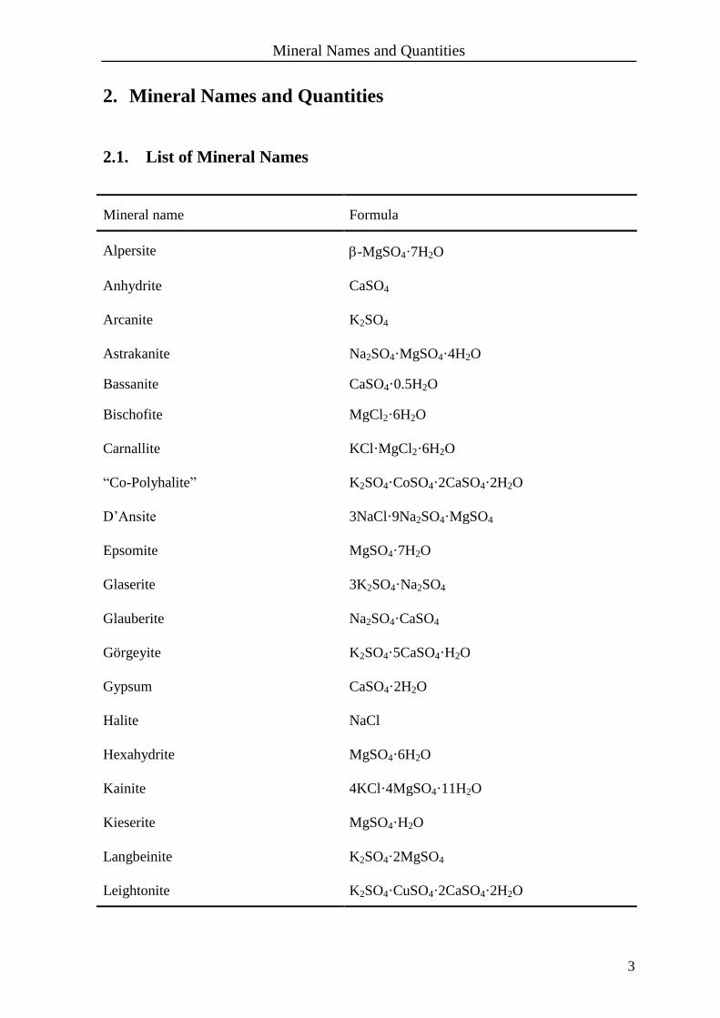
2.1. List of Mineral Names
Mineral name Formula
Alpersite -MgSO4·7H2O
Anhydrite CaSO4
Arcanite K2SO4
Astrakanite Na2SO4·MgSO4·4H2O
Bassanite CaSO4·0.5H2O
Bischofite MgCl2·6H2O
Carnallite KCl·MgCl2·6H2O
“Co-Polyhalite” K2SO4·CoSO4·2CaSO4·2H2O
D’Ansite 3NaCl·9Na2SO4·MgSO4
Epsomite MgSO4·7H2O
Glaserite 3K2SO4·Na2SO4
Glauberite Na2SO4·CaSO4
Görgeyite K2SO4·5CaSO4·H2O
Gypsum CaSO4·2H2O
Halite NaCl
Hexahydrite MgSO4·6H2O
Kainite 4KCl·4MgSO4·11H2O
Kieserite MgSO4·H2O
Langbeinite K2SO4·2MgSO4
Leightonite K2SO4·CuSO4·2CaSO4·2H2O
Mineral Names and Quantities
4
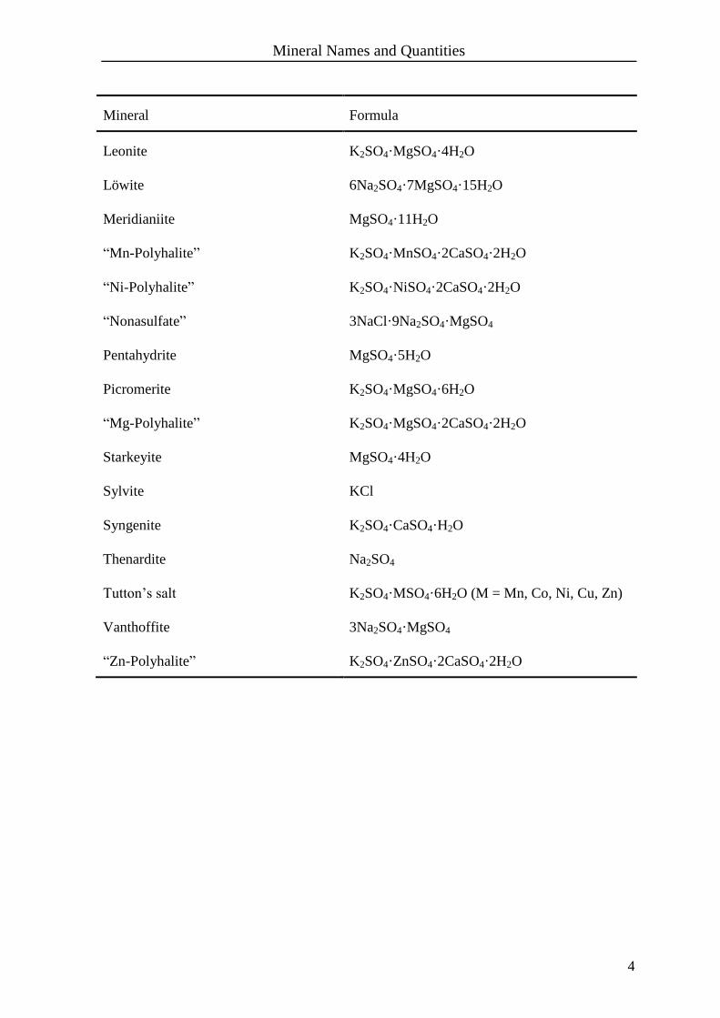
Mineral Formula
Leonite K2SO4·MgSO4·4H2O
Löwite 6Na2SO4·7MgSO4·15H2O
Meridianiite MgSO4·11H2O
“Mn-Polyhalite” K2SO4·MnSO4·2CaSO4·2H2O
“Ni-Polyhalite” K2SO4·NiSO4·2CaSO4·2H2O
“Nonasulfate” 3NaCl·9Na2SO4·MgSO4
Pentahydrite MgSO4·5H2O
Picromerite K2SO4·MgSO4·6H2O
“Mg-Polyhalite” K2SO4·MgSO4·2CaSO4·2H2O
Starkeyite MgSO4·4H2O
Sylvite KCl
Syngenite K2SO4·CaSO4·H2O
Thenardite Na2SO4
Tutton’s salt K2SO4·MSO4·6H2O (M = Mn, Co, Ni, Cu, Zn)
Vanthoffite 3Na2SO4·MgSO4
“Zn-Polyhalite” K2SO4·ZnSO4·2CaSO4·2H2O

Mineral Names and Quantities
5
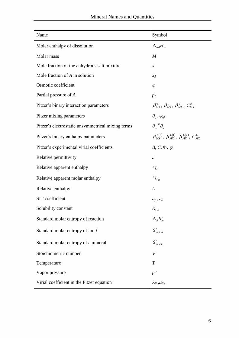
2.2. Quantities
Name Symbol
Activity a
Activity coefficient
Amount of substance n
Avogadro’s number N0
Boltzmann’s constant k
Calculated activity coefficient calc
Calculated osmotic coefficient calc
Debye-Hückel coefficients A , A , AL
Density d
Deviation of the activity coefficient = calc - exp
Deviation of the osmotic coefficient = calc - exp
Electronic charge e
Equilibrium constant K
Excess Gibbs energy exG
Experimental activity coefficient exp
Experimental osmotic coefficient exp
Fractional deviation of the activity coefficient /
Fractional deviation of the osmotic coefficient
Gas constant R
Ionic charge z
Mass m
Molal ionic strengths Im
Molality m
Molar enthalpy of dissolution at infinite dilution msolH
Molar enthalpy of dilution mdilH
Mineral Names and Quantities
6
Name Symbol
Molar enthalpy of dissolution msolH
Molar mass M
Mole fraction of the anhydrous salt mixture x
Mole fraction of A in solution xA
Osmotic coefficient
Partial pressure of A pA
Pitzer’s binary interaction parameters 210 ,, MXMXMX , MXC
Pitzer mixing parameters ij, ijk
Pitzer’s electrostatic unsymmetrical mixing terms ij, Eij
Pitzer’s binary enthalpy parameters 210 ,, L
MX
L
MX
L
MX , L
MXC
Pitzer’s experimental virial coefficients B, C, ,
Relative permittivity
Relative apparent enthalpy L
Relative apparent molar enthalpy mL
Relative enthalpy L
SIT coefficient , L
Solubility constant Ksol
Standard molar entropy of reaction mR S
Standard molar entropy of ion i
ionmS ,
Standard molar entropy of a mineral
min,mS
Stoichiometric number
Temperature T
Vapor pressure p°
Virial coefficient in the Pitzer equation ij ,ijk

Literature Review
7
3. Literature Review
3.1. Basic Thermodynamics of Electrolyte Solutions
3.1.1. Activity
Electrolyte solutions show the thermodynamic behavior of ideal as well as of real
solutions. In case of dilute solutions, they can be described by Raoult’s law [1] for ideal
solutions with increasing precision as infinite dilution is approached.
AAA pxp [1]
Here, pA is the partial pressure of the compound A above the solution, Ap the vapor
pressure of the pure substance A and xA the mole fraction of A in the solution.
However, few solutions of electrolytes occurring in Nature behave ideally solutions. This
is due to interactions between the species in solution. Therefore, it is necessary to introduce
a quantity to specify how much the solution differs from ideal behavior. For this reason,
iii ma [2]
the activity coefficient is introduced, where ai denotes the activity of substance i and mi
the molality of i. For the limiting case of infinitely dilute solution i = 1, and then ai = mi,
the ideal solution.
3.1.2. Osmotic Coefficients
For non-electrolytes the activity coefficients of solute and solvent are of similar magnitude.
However, in aqueous electrolyte solutions the activity coefficients differ significantly for
water and the dissolved electrolyte in dilute solutions. With increasing concentration of
solution, the activity coefficient of the solute decreases rapidly, unlike the activity
coefficient of water. Here, the change is small. Describing the behavior of the solution with
the activity of the solvent makes it therefore difficult. For this reason, the osmotic
coefficient is introduced. Water activity wa and osmotic coefficient are related by
w
i
iw
amM
ln1000
[3]
where wM is the molar mass of water and i refers to any kind of ion.

Literature Review
8
3.1.3. Solubility Constants
Solid-liquid equilibria play a major role in geochemical processes. The solubility constant
Ksol describes the equilibrium depending on the component, temperature and pressure. For
a mineral MX · xH2O, the solubility constant is defined as
WXM
XM WXMWsol aaaOHXMK
2 [4]
Using equation [2], this gives in logarithmic form
)ln()ln()ln(ln 2 WWXXXMMMWsol ammOHXMKXM
[5]
where denotes the stoichiometric number. The indices M, X and W represent the cation,
anion and water, respectively.
3.1.4. Relative Apparent Molar Enthalpy
The partial molar enthalpy of a substance i is defined as
jnTpi
imn
HH
,,
,
[6]
at constant pressure, temperature and amount of compound j . The partial molar enthalpy
is dependent on the composition of the mixture.
In most measurements, it is not possible to separate the enthalpy into separate contributions
by the solvent and the solute. However, the enthalpy of the solvent under standard
conditions is well known for most solvents. For this reason, the measured quantity is
divided into the standard partial molar enthalpy of the solvent 1,mH and the remainder is
related to the solute. Therefore only the apparent molar enthalpy of the solute 2,mH is
given by the following equation.
2
1,1
2
2,n
HnH
n
HHH
m
m
[7]
In equation [7] the subscript 1 indicates the solvent and subscript 2 the solute. With this in
mind, the reference of the apparent molar enthalpy is the standard molar enthalpy of the
solvent. At infinite dilution, the partial molar enthalpy
2,mH and the apparent molar
enthalpy are identical.
2,2,2
02
lim mmn
HHH
[8]
Because the enthalpy can not be determined as an absolute quantity, it is necessary to relate
the measured enthalpy to a standard state. For solvents, it is the pure substance, and for
Literature Review
9
electrolyte solutions, the infinitely diluted solution is defined as the standard state. The
relative partial molar enthalpy imL , of a substance i is given by
imimim HHL ,,, [9]
in terms of the partial molar enthalpy imH , and the standard partial molar enthalpy imH , .
From these considerations the relative apparent molar enthalpy 2,mL of the electrolyte can
be derived. With the expression for the enthalpy 2,21,1 mm HnHnH the following
results from equation [7].
1,12,21,12,2 mmmm HnHnHnHn [10]
Addition of 2,22,2 mm HnHn , and the introduction of equation [9] lead to
equation [11].
2,21,12,22,2 mmmm LnLnHnHn [11]
From this conclusion, equation [12] and [13] follow for the relative apparent molar
enthalpy.
2,21,12,22,22,2 mmmmm LnLnHnHnLn [12]
LLn m 2,2
[13]
3.2. Ion Interaction Models
In describing electrolyte solutions, long-range coulombic as well as short-range specific
ion-ion and ion-solute forces have to be considered. For the limiting case of infinitely
dilute solutions, the deviation from ideal behavior due to the coulombic forces between
cation and anion can be described with the Debye-Hückel limiting law. If the radii of the
ions are taken into account, calculations up to 0.1 molal can be realized with the extended
Debye-Hückel equation. An empirical extension of the Debye-Hückel theory was provided
by Davies. His equation allows the calculation of the activity coefficient with high
accuracy for ionic strengthss up to 0.1 molal (11).
The equations describe only the long-range coulombic interactions of the ions. However, in
concentrated solutions short-range interactions dominate. Therefore, models that deal with
solutions above 0.1 molal divide the ion interactions into long-range and short-range term.
For the long-range interactions, the Debye-Hückel approach is generally applied. The

Literature Review
10
short-range forces are expressed by empirical functions or through a theoretical molecular
approach.
An example of the empirical extension of the Debye-Hückel theory to high ionic strengths
is the equation of Bromley (11).
For aqueous solutions, the Pitzer equations have been employed successfully to represent
data within experimental error from dilute solutions up to ionic strengths of around six for
single and mixed electrolyte solutions. The theory is based on the extension of the Debye-
Hückel term with a virial equation.
A simpler model is the Specific Ion Interaction Theory (SIT). A linear extension is added
to the Debye-Hückel term. The assumption of like-ion repulsion leads to only one binary
parameter for a pure electrolyte in water. For that reason, the model encounters difficulties
at higher concentrations. However, the model is applied widely and successfully for the
extrapolation of thermodynamic data to infinite dilution.
Local composition models such as the extended Universal Quasichemical (UNIQUAC)
model and the nonrandom, two-liquid (NRTL) model consider, beside the long-range
forces, not only short-range interactions between the ions, but also interactions with the
solvent. Therefore, these models can be employed for calculations involving mixed solvent
systems. Nevertheless, additional parameters such as volume and surface area of the ions
and of the solvent molecules are required.
So far, neither of the models allows calculations at high ionic strengths.
3.2.1. The Pitzer Equations
The following section is intended to provide only a brief outline of the Pitzer equations.
The approach classifies the ion interactions in solution into two parts, coulombic forces
being effective on relatively long-range, and the specific short-range forces. The long-
range electrostatic part is described on the basis of the extended Debye-Hückel theory. It
depends mainly on the molal ionic strengths Im and the ionic charge z. The short-range
interactions are described with a virial type equation (12).
The excess Gibbs energy Gex
is expressed as
i j k
ijkkji
i j
mijjim
ex
mmmImmIf
RT
G
wm
[14]
where wm is the mass of water, R is the gas constant and T the temperature, f (Im) refers to
the Debye-Hückel term, and mi, mj and mk denote the molality of the different species in
Literature Review
11
solution; ij and ijk express the virial coefficients. The molal ionic strengths Im is given by
the following equation.
i
iim zmI 2
2
1 [15]
The relation between the excess Gibbs energy, the osmotic coefficient and the activity
coefficient is shown in equation [16].
i
ii
w
ex
mRTG
ln1
m
[16]
In order to treat mixed electrolytes, the osmotic coefficient and the activity coefficient
derivations of the excess Gibbs energy lead to the following expressions.
a a c
caacaaaa
c c a
accacccc
c a
cacaac
m
i
i mmm
mmmZCBmm
Ib
IA
m
'
'''
'
'''
23
121
[17]
a c
caacM
a a
Maaaa
a c a
McaaMccMaMaaMM
Cmmzmm
mmZCBmFz
'
''
2 22ln
[18]
a c
caacX
c c
Xcccc
c a c
XaccXaacXcXcXX
Cmmzmm
mmZCBmFz
'
''
2 22ln
[19]
Here, c and c’ denote cations in general. Similarly, the a and a’ indicate anions. The
summation index c implies the sum over all cations and the double summation index
c < c’ stands for the sum of distinguishable pairs of dissimilar cations. For the summation
indices of the anions, analogous definitions apply. The individual ion qualities ij and ijk
are rewritten as the experimentally determinable quantities B, C, and .
In equation [18] and [19], function F is defined as
a a
aaaa
c c
cccc
c a
caacm
m
m
mmmm
BmmIbbIb
IAF
'
'
''
'
'
''
'1ln2
1
[20]

Literature Review
12
with B’ and ’ as ionic strength derivations of B and . In the Debye-Hückel term
m
m
mIb
bIb
IA 1ln
2
1 with b = 1.2, A denotes the Debye-Hückel slope, that
can be calculated using the following expression.
23221
0
1000
2
3
1
kT
edNA w
[21]
The coefficient depends on the density of water dw and the relative permittivity of water .
Further notations refer to Avogadro’s number N0, the electronic charge e, and Boltzmann’s
constant k.
The binary virial coefficient, BMX, describes the short-range interactions between two ions.
Pitzer (12) defines BMX dependent on the ionic strength as
mm I
MX
I
MXMXMX eeB 21 210
[22]
mMXmMXMXMX IgIgB 2
2
1
10 [23]
m
mMXmMX
MXI
IgIgB
2
'2
1
'1
'
[24]
where the functions g and g’ are given by
xexx
xg 112
2 [25]
xe
xx
xxg
211
2 2
2
' [26]
withmIx . The values 1 and 2 were found empirically (12). For 1-1 electrolytes,
1 is 2. In the case of higher valence types, such as 2-2 electrolytes, Pitzer assigned
1 = 1.4 and 2 = 12.
The third virial coefficient CMX is assumed to be independent of ionic strength, since the
experimentally recognized dependency is small. Regarding the understanding of the
coefficient, CMX expresses the interactions between three ions of M and X. Usually, CMX is
tabulated as MXC , related by equation [27]
Literature Review
13
XM
MXMX
zz
CC
2
[27]
In terms with CMX (equation [17]), concentration dependence is given by the function
i
ii zmZ [28]
where 0
MX , 1
MX , 2
MX and MXC are referred to as binary interaction parameters of the salt
MX and depend on temperature and pressure. The parameter 2
MX is used to describe the
ion association between higher valency types of electrolytes. Therefore, it does not apply
for lower valency types generally.
For mixed electrolytes, the terms ij and ijk are added to the equation. The parameter ij
describes the interaction between two different ions i and j of like signs. The equations of
the second virial mixing coefficient are as follows.
mij
E
mij
E
ijij III ' [29]
mij
E
ijij I [30]
mijE
ij I'' [31]
For equation [29] and [30], ij is the only adjustable parameter and has to be taken into
account for each pair of anions and each pair of cations. Expressions mij
E I , and
mij
E
m II ' are the unsymmetrical electrostatic mixing terms. Equations calculating these
terms are derived by Pitzer (12). They will not be described in more detail here, but they
depend on the charges of the ions i and j, the total ionic strength, the pressure and the
temperature. Both parameters are zero, when i and j are of the same charge. The parameter
ij also shows ionic strengths dependence, which is small and taken to be negligible.
The third virial mixing coefficient ijk characterizes the interactions between three
different ions i, j and k. This means two different cations and one anion or two different
anions and one cation interact. The Pitzer mixing parameters ij and ijk depend also on
temperature and pressure.
The binary as well as the mixing parameters are obtained usually from activity coefficients
or from osmotic coefficients of unsaturated pure and mixed electrolyte solutions,
respectively. Solubility studies provide also activity data, which can be used if the
thermodynamic solubility constant of the solid phase is known with sufficient accuracy,

Literature Review
14
equilibration is fast and formation of solid solutions can be excluded. Since solubility
studies are extensively available for mixed electrolyte solutions, mixing parameters can be
estimated from these data.
Typically, binary interaction parameters are determined first. With these parameters, the
Pitzer mixing parameters are determined.
3.2.1.1. Temperature Dependence of Pitzer’s Ion Interaction Parameters
Calculations of the osmotic coefficient and the activity coefficient at different temperatures
require information about the interaction parameters at these temperatures.
They can be obtained from experimental data for osmotic coefficients or activity
coefficients at different temperatures, and also from enthalpy and heat capacity data. The
equations necessary are derived from the excess Gibbs energy Gex
. The thermodynamic
equation for the relative enthalpy L is given by equation [32].
mp
ex
T
TGTL
,
2
[32]
Experimental measurements of enthalpy usually provide the relative apparent molar
enthalpy of the solute Lm, 2. Applying equation [16] to the derivations of equation [32]
results in the following.
L
MXMM
L
MXXMmL
XMm CzmmBRTbI
b
AzzL 2221
2, 21ln
2
[33]
with
m
L
MXm
L
MX
L
MX
Ip
MXL
MX IgIgT
BB 2
2
1
10
,
[34]
2,1,0,
i
Tp
i
MXLi
MX
[35]
and
21
2 XM
pMX
p
MXL
MX
zz
TC
T
CC
[36]
The Debye-Hückel slope of the enthalpy is derived from equation [37].
p
LT
ARTA
24 [37]
Literature Review
15
From L
MXB and L
MXC , the temperature dependence of the coefficients BMX and CMX can be
determined. The calculation of these parameters requires the relative apparent molar
enthalpy of the solute Lm, 2, which can be computed from the molar heat of dilution dilHm
using
2,2, mmmdil LLH [38]
where 2,mL is the relative apparent molar enthalpy of the solute before dilution and 2,mL
the relative apparent molar enthalpy of the solute after dilution.
From molar heat of dissolution solHm measurements the relative apparent molar enthalpy
can be calculated by
msolmsolm HHL 2,
[39]
presuming the molar enthalpy of dissolution at infinite dilution msolH is known.
3.2.1.2. Relative Molar Enthalpy of Single Electrolytes on the Basis of Pitzer’s
Equation
The relative apparent molar enthalpy can also be written as
2,21,12,2 mmm LnLnLn [40]
using Lm,1 and Lm,2. The relative molar enthalpy of the solvent is denoted by 1, and the
relative molar enthalpy of the solute denoted by 2; n represents the amount of substance.
The dependence of the relative molar enthalpy from the osmotic coefficient is as follows.
T
MmRTLm
1000
12
1, [41]
With the Pitzer approach, equation [42] can be obtained for water in solutions of an
electrolyte NX (13).
L
NXNN
IL
NX
L
NXXN
m
mLW
m mCzemRTI
IAML m
22
2.1121000
10222
3
1, [42]
The relative molar enthalpy of the solute depends on the activity coefficient according to
equation [43].
TRTLm
ln2
2, [43]
Literature Review
16
For an ion M present at trace concentrations in a solution of an electrolyte NX, and using
Pitzer’s equation, the following expression is derived.
L
NXXNM
L
MXXXNNX
p
MNX
X
p
MN
N
L
MX
L
MXX
m
L
NXXNMm
m
mLMMm
CmmzRTCzmzmmRT
Tm
TmRTxgmRT
I
xgmmzRTIb
bIb
IAzL
22
2102
1222
,2,
22
)('1ln
2
14
[44]
Here, AL refers to the Debye-Hückel slope (equation [37]), g and g’ are defined in
equations [25] and [26] and Lij
0 , Lij
1 and L
ijC are the binary enthalpy parameters. The
parameters MN and MNX are explained in section 3.2.1.
3.2.2. The SIT Model
The Specific Ion Interaction Theory (SIT) also separates electrostatic long-range and
non-electrostatic short-range interactions. In dilute solutions, the long-range interactions
described by the Debye-Hückel term dominate. For higher concentrations, the short-range
interactions have to be taken into account as well. In the SIT model this is realized by
adding a linear expression to the Debye-Hückel term (equation [45]) (13), where A is
k
k
m
mi
i mki
I
IAz,
5.11
ln
2
[45]
the limiting Debye-Hückel law slope and is related to A (equation [21]) by AA 3 (14).
The specific short-range interactions between the species i and k are expressed by the
coefficient (i, k). The ion interaction coefficient is assumed to be independent of
concentration, and results in the identity ikki ,, for all strong n : n electrolytes.
Another assumption considers the specific interaction between ions of same charge. Here,
the ion interaction coefficient (i, k) is zero, which is explained by the electrostatic
repulsion of these ions leading to small short-range forces between them.
Literature Review
17
3.2.2.1. Relative Molar Enthalpy of Single Electrolytes on the Basis of the SIT Model
The corresponding equation of the relative molar enthalpy of water in a solution of the
electrolyte NX using the SIT model is
XNmzRT
t
ttAM
L LNNLW
m ,1
ln2
5.12
3
1000
22
31, [46]
with mIt 5.11 (13). The coefficient L denotes the enthalpy parameter of the SIT
model.
In solution of an ionic medium of electrolyte NX, the relative molar enthalpy of an ion i,
Lm,2,i, at trace concentration can be determined with
)(
5.114
3 2
2
,2, ijmRT
I
IzAL Li
m
miL
iim
[47]
when AL is defined as in equation [37].

Literature Review
18
3.3. Characterization of Salt-Water Systems
3.3.1. Binary Systems MX+
/ SO42-
// H2O
(M = K, Ca, Mg, Mn, Co, Ni, Cu, Zn)
In this chapter, an overview of the literature data relevant for this study is provided. The
aim is the identification of gaps in the data in order to schedule necessary experimental
work.
3.3.1.1. Solubility
Extensive studies of the binary systems MX+
/ SO42-
// H2O (K, Ca, Mg, Mn, Co, Ni, Cu,
Zn) are provided in the literature within the considered temperature range from 298 K to
323 K.
In this study, the binary system K+ / SO4
2- // H2O is the only one with a univalent cation,
where arcanite (K2SO4) is the stable solid phase in solutions in the required temperature
range (Figure 1).
260 280 300 320 340 360 380 400
0.0
0.2
0.4
0.6
0.8
1.0
1.2
1.4
1.6
1.8
K2SO
4
Ice
m (
K2S
O4)
/ mol
kg
-1
T / K
Figure 1: Potassium sulfate-water system (15-49); -ice, -K2SO4, curves-estimated solubility
lines drawn by eye.
All of the bivalent metal sulfates included in this work form salt hydrates. Calcium sulfate
crystallizes as gypsum (CaSO4·2H2O), bassanite (CaSO4·0.5H2O) and anhydrite (CaSO4)
from aqueous solutions (Figure 2). The temperature dependence of the solubility of these
Literature Review
19
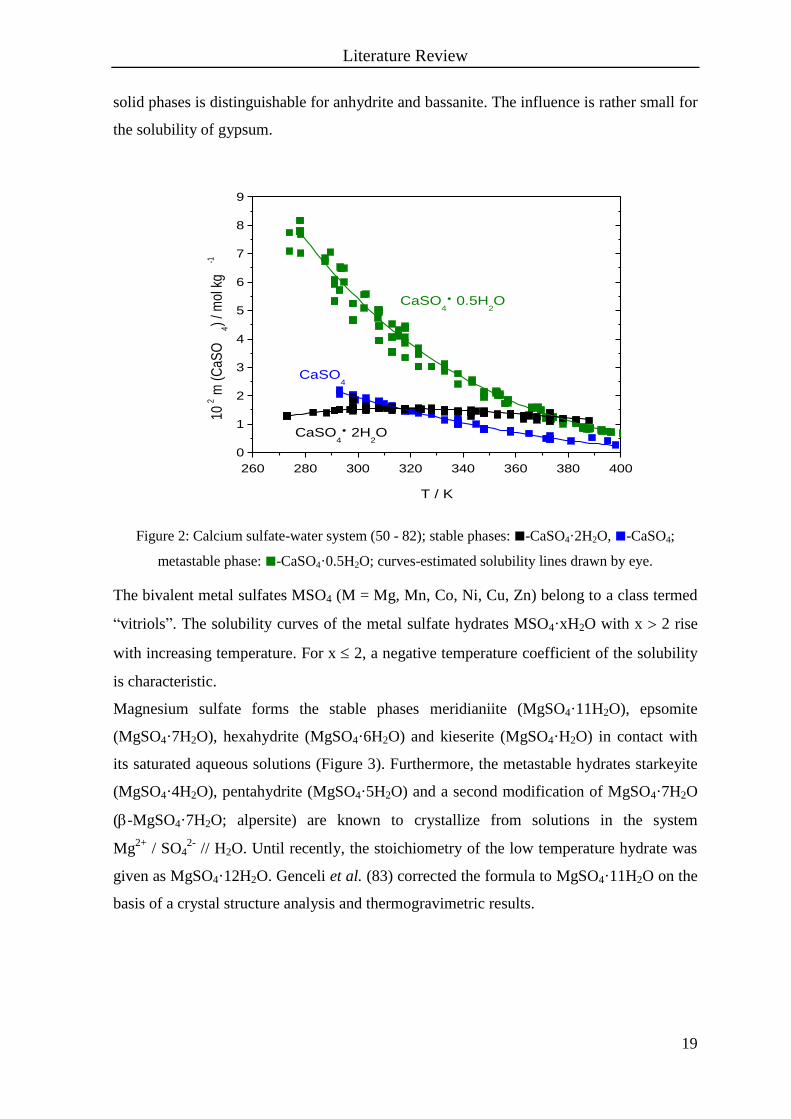
solid phases is distinguishable for anhydrite and bassanite. The influence is rather small for
the solubility of gypsum.
260 280 300 320 340 360 380 400
0
1
2
3
4
5
6
7
8
9
CaSO4
CaSO4
0.5H2O
CaSO4
2H2O
102 m
(C
aSO
4)
/ mol
kg
-1
T / K
Figure 2: Calcium sulfate-water system (50 - 82); stable phases: -CaSO4·2H2O, -CaSO4;
metastable phase: -CaSO4·0.5H2O; curves-estimated solubility lines drawn by eye.
The bivalent metal sulfates MSO4 (M = Mg, Mn, Co, Ni, Cu, Zn) belong to a class termed
“vitriols”. The solubility curves of the metal sulfate hydrates MSO4·xH2O with x 2 rise
with increasing temperature. For x 2, a negative temperature coefficient of the solubility
is characteristic.
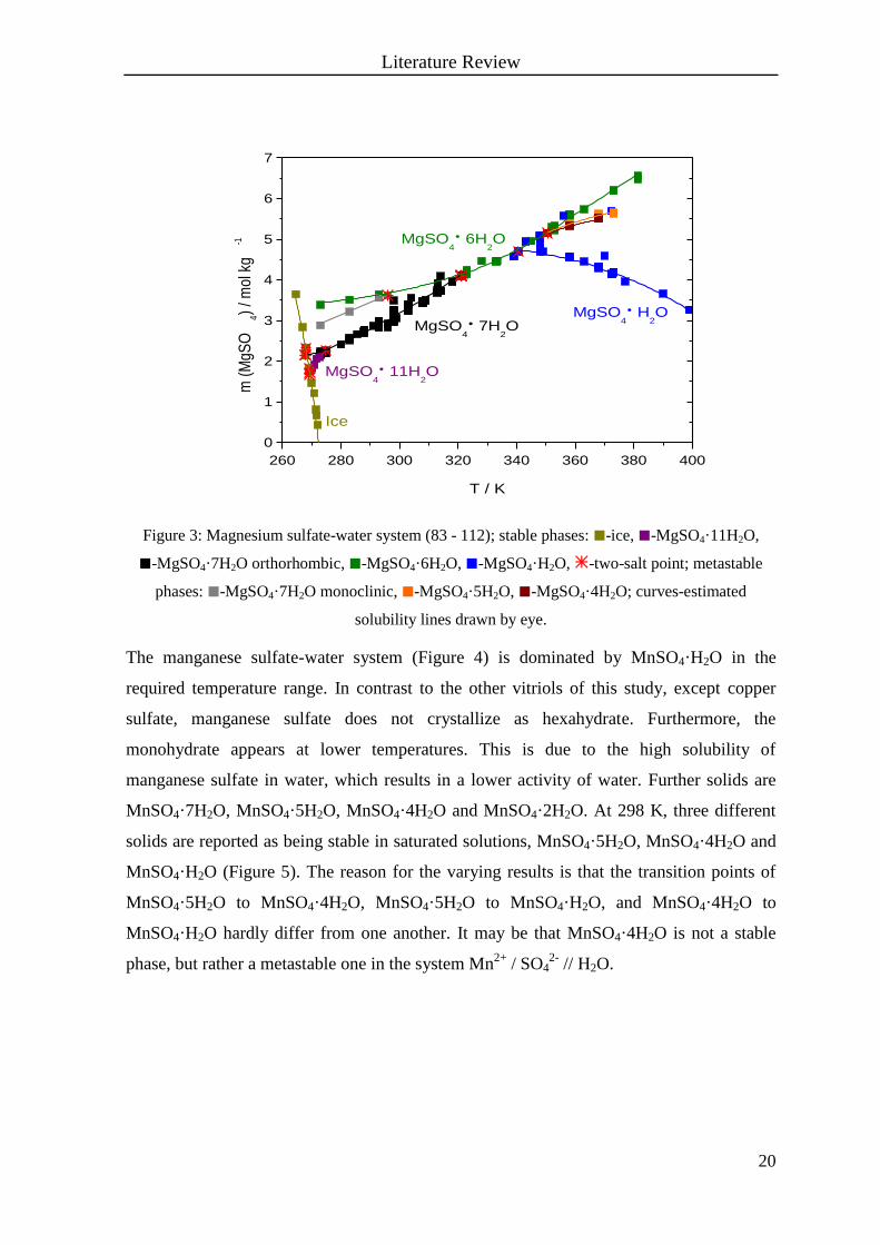
Magnesium sulfate forms the stable phases meridianiite (MgSO4·11H2O), epsomite
(MgSO4·7H2O), hexahydrite (MgSO4·6H2O) and kieserite (MgSO4·H2O) in contact with
its saturated aqueous solutions (Figure 3). Furthermore, the metastable hydrates starkeyite
(MgSO4·4H2O), pentahydrite (MgSO4·5H2O) and a second modification of MgSO4·7H2O
(-MgSO4·7H2O; alpersite) are known to crystallize from solutions in the system
Mg2+
/ SO42-
// H2O. Until recently, the stoichiometry of the low temperature hydrate was
given as MgSO4·12H2O. Genceli et al. (83) corrected the formula to MgSO4·11H2O on the
basis of a crystal structure analysis and thermogravimetric results.
Literature Review
20
260 280 300 320 340 360 380 400
0
1
2
3
4
5
6
7
Ice
MgSO4
11H2O
MgSO4
6H2O
MgSO4
7H2O
MgSO4
H2O
m (
MgS
O4)
/ mol
kg
-1
T / K
Figure 3: Magnesium sulfate-water system (83 - 112); stable phases: -ice, -MgSO4·11H2O,
-MgSO4·7H2O orthorhombic, -MgSO4·6H2O, -MgSO4·H2O, -two-salt point; metastable
phases: -MgSO4·7H2O monoclinic, -MgSO4·5H2O, -MgSO4·4H2O; curves-estimated
solubility lines drawn by eye.
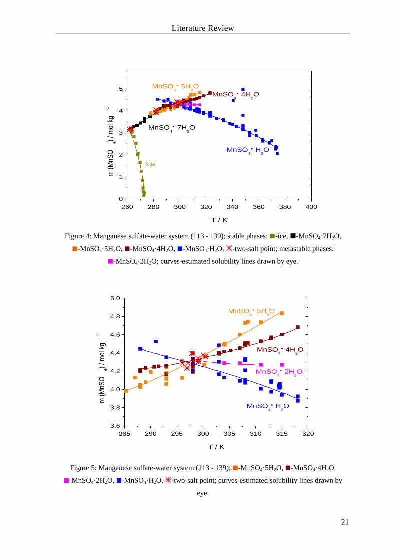
The manganese sulfate-water system (Figure 4) is dominated by MnSO4·H2O in the
required temperature range. In contrast to the other vitriols of this study, except copper
sulfate, manganese sulfate does not crystallize as hexahydrate. Furthermore, the
monohydrate appears at lower temperatures. This is due to the high solubility of
manganese sulfate in water, which results in a lower activity of water. Further solids are
MnSO4·7H2O, MnSO4·5H2O, MnSO4·4H2O and MnSO4·2H2O. At 298 K, three different
solids are reported as being stable in saturated solutions, MnSO4·5H2O, MnSO4·4H2O and
MnSO4·H2O (Figure 5). The reason for the varying results is that the transition points of
MnSO4·5H2O to MnSO4·4H2O, MnSO4·5H2O to MnSO4·H2O, and MnSO4·4H2O to
MnSO4·H2O hardly differ from one another. It may be that MnSO4·4H2O is not a stable
phase, but rather a metastable one in the system Mn2+
/ SO42-
// H2O.
Literature Review
21
260 280 300 320 340 360 380 400
0
1
2
3
4
5
MnSO4
4H2O
MnSO4
H2O
MnSO4
5H2O
MnSO4
7H2O
Ice
m (
MnS
O4)
/ mol
kg
-1
T / K
Figure 4: Manganese sulfate-water system (113 - 139); stable phases: -ice, -MnSO4·7H2O,
-MnSO4·5H2O, -MnSO4·4H2O, -MnSO4·H2O, -two-salt point; metastable phases:
-MnSO4·2H2O; curves-estimated solubility lines drawn by eye.
285 290 295 300 305 310 315 320
3.6
3.8
4.0
4.2
4.4
4.6
4.8
5.0
MnSO4
2H2O
MnSO4
4H2O
MnSO4
H2O
MnSO4
5H2O
m (
MnS
O4)
/ mol
kg
-1
T / K
Figure 5: Manganese sulfate-water system (113 - 139); -MnSO4·5H2O, -MnSO4·4H2O,
-MnSO4·2H2O, -MnSO4·H2O, -two-salt point; curves-estimated solubility lines drawn by
eye.

Literature Review
22
Investigations of the binary system cobalt sulfate-water (Figure 6) show the existence of
the solid phases CoSO4·7H2O, CoSO4·6H2O, CoSO4·4H2O, CoSO4·2H2O and
CoSO4·H2O, of which the tetrahydrate and the dihydrate form metastable solids.
260 280 300 320 340 360 380 400
0
1
2
3
4
5
CoSO4
H2O
CoSO4
6H2O
CoSO4
7H2O
Ice
m (
CoS
O4)
/ mol
kg
-1
T / K
Figure 6: Cobalt sulfate-water system (97, 140 - 166); stable phases: -ice, -CoSO4·7H2O,
-CoSO4·6H2O, -CoSO4·H2O, -two-salt point; metastable phases: -CoSO4·4H2O,
-CoSO4·2H2O; curves-estimated solubility lines drawn by eye.
Nickel sulfate presents all integer hydrates from one to seven, though only NiSO4·7H2O,
NiSO4·6H2O and NiSO4·H2O are thermodynamic stable in contact with aqueous solutions.
As can be seen in Figure 7, two modifications of NiSO4·6H2O can be distinguished,
-NiSO4·6H2O and β-NiSO4·6H2O; -NiSO4·6H2O crystallizes in the tetragonal system
and -NiSO4·6H2O in the monoclinic system.
Copper sulfate is the vitriol that differs from the others in this work the most. In the
solubility diagram, no heptahydrate or hexahydrate appears (Figure 8). Unlike the other
vitriols, CuSO4·5H2O and CuSO4·3H2O represent the stable phases in the system
Cu2+
/ SO42-
// H2O.

Literature Review
23
260 280 300 320 340 360 380 400
0
1
2
3
4
5
6
NiSO4
H2O
- NiSO4
6H2O
- NiSO4
6H2O
NiSO4
7H2O
Ice
m (
NiS
O4)
/ mol
kg
-1
T / K
Figure 7: Nickel sulfate-water system (167 - 180); stable phases: -ice, -NiSO4·7H2O,
--NiSO4·6H2O, -β-NiSO4·6H2O, -NiSO4·H2O, -two-salt point; metastable phases:
-NiSO4·5H2O, -NiSO4·4H2O, -NiSO4·3H2O, -NiSO4·2H2O; curves-estimated solubility
lines drawn by eye.
260 280 300 320 340 360 380 400
0
1
2
3
4
5
Ice
CuSO4
5H2O
CuSO4
3H2O
m (
CuS
O4)
/ mol
kg
-1
T / K
Figure 8: Copper sulfate-water system (181 - 202); -ice, -CuSO4·5H2O, -CuSO4·3H2O,
-two-salt point; curves-estimated solubility lines drawn by eye.
Literature Review
24
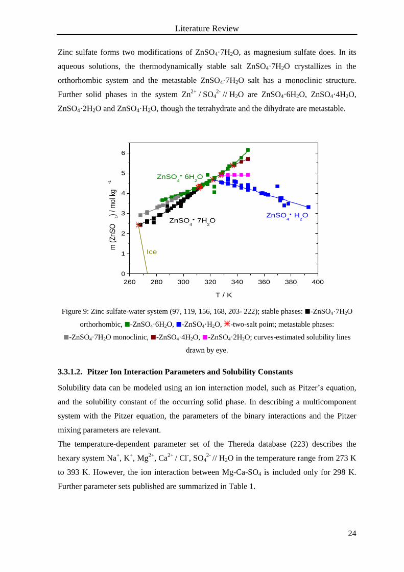
Zinc sulfate forms two modifications of ZnSO4·7H2O, as magnesium sulfate does. In its
aqueous solutions, the thermodynamically stable salt ZnSO4·7H2O crystallizes in the
orthorhombic system and the metastable ZnSO4·7H2O salt has a monoclinic structure.
Further solid phases in the system Zn2+
/ SO42-
// H2O are ZnSO4·6H2O, ZnSO4·4H2O,
ZnSO4·2H2O and ZnSO4·H2O, though the tetrahydrate and the dihydrate are metastable.
260 280 300 320 340 360 380 400
0
1
2
3
4
5
6
Ice
ZnSO4
7H2O
ZnSO4
6H2O
ZnSO4
H2O
m (
ZnS
O4)
/ mol
kg
-1
T / K
Figure 9: Zinc sulfate-water system (97, 119, 156, 168, 203- 222); stable phases: -ZnSO4·7H2O
orthorhombic, -ZnSO4·6H2O, -ZnSO4·H2O, -two-salt point; metastable phases:
-ZnSO4·7H2O monoclinic, -ZnSO4·4H2O, -ZnSO4·2H2O; curves-estimated solubility lines
drawn by eye.
3.3.1.2. Pitzer Ion Interaction Parameters and Solubility Constants
Solubility data can be modeled using an ion interaction model, such as Pitzer’s equation,
and the solubility constant of the occurring solid phase. In describing a multicomponent
system with the Pitzer equation, the parameters of the binary interactions and the Pitzer
mixing parameters are relevant.
The temperature-dependent parameter set of the Thereda database (223) describes the
hexary system Na+, K
+, Mg
2+, Ca
2+ / Cl
-, SO4
2- // H2O in the temperature range from 273 K
to 393 K. However, the ion interaction between Mg-Ca-SO4 is included only for 298 K.
Further parameter sets published are summarized in Table 1.

Literature Review
25
Table 1: Parameter sets based on the Pitzer approach
Ions considered in the parameter set Temperature
range
Ref.
Na+, K
+, Mg
2+, Ca
2+ / Cl
-, SO4
2- // H2O 298 K 224
H+, Na
+, K
+, Mg
2+, Ca
2+ / OH
-, Cl
-, SO4
2-, CO3
2- // CO2, H2O 298 K 225
Na+, K
+, Ca
2+ / Cl
-, SO4
2- // H2O 273 K – 523 K 226
H+, Na
+, K
+ / OH
-, Cl
-, SO4
2-, HSO4
-// H2O 273 K – 523 K 227
H+, Na
+, K
+, Ca
2+ / OH
-, Cl
-, SO4
2-, HSO4
-// H2O 273 K – 523 K 228
Na+, K
+, Mg
2+ / Cl
-, SO4
2- // H2O 298 K – 363 K 229
As can be seen, none of these includes magnesium and calcium ions at the same time at
elevated temperatures, as the database of Thereda (223) does. For that reason, this work is
based on the Thereda database.
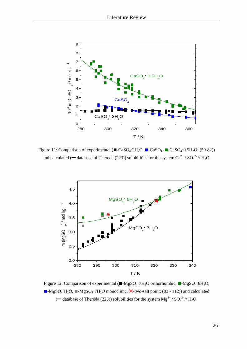
With Pitzer’s equation and the parameters of Thereda, the temperature-dependent
solubilities of the major solid phases of the systems MX+
/ SO42-
// H2O (K, Ca, Mg) are
represented mostly within the limits of experimental accuracy (Figure 10 to Figure 12).
280 290 300 310 320 330 340
0.4
0.6
0.8
1.0
1.2
K2SO
4
m (
K2S
O4)
/ mol
kg
-1
T / K
Figure 10: Comparison of experimental (-K2SO4; (15 - 49)) and calculated ( database of
Thereda (223)) solubilities for the system K+ / SO4
2- // H2O.
Literature Review
26
280 300 320 340 360
0
1
2
3
4
5
6
7
8
9
CaSO4
CaSO4
0.5H2O
CaSO4
2H2O
102 m
(C
aSO
4)
/ mol
kg
-1
T / K
Figure 11: Comparison of experimental (-CaSO4·2H2O, -CaSO4, -CaSO4·0.5H2O; (50-82))
and calculated ( database of Thereda (223)) solubilities for the system Ca2+
/ SO42-
// H2O.
280 290 300 310 320 330 340
2.0
2.5
3.0
3.5
4.0
4.5
MgSO4
6H2O
MgSO4
7H2O
m (
MgS
O4)
/ mol
kg
-1
T / K
Figure 12: Comparison of experimental (-MgSO4·7H2O orthorhombic, -MgSO4·6H2O,
-MgSO4·H2O, -MgSO4·7H2O monoclinic, -two-salt point; (83 - 112)) and calculated
( database of Thereda (223)) solubilities for the system Mg2+
/ SO42-
// H2O.

Literature Review
27
The heavy metal sulfate systems M2+
/ SO42-
// H2O (M = Mn, Co, Ni, Cu, Zn) are not
described thermodynamically as well as the systems discussed above. In the literature,
Pitzer parameter sets derived from the osmotic coefficients and activity coefficients of
MSO4 solutions are provided only for one temperature, 298 K. The requirement of validity,
up to high concentrations of the metal sulfate, and the use of 1 = 1.4 and 2 = 12, limit the
selection of the parameter sets as well.
Published Pitzer parameters of the ion interaction Mn2+
- SO42-
are summarized in Table 2.
Table 2: Pitzer parameters for Mn2+
-SO42-
at 298 K; 1 = 1.4, 2 = 12.
β0
β1 β
2 C
mmax / mol kg-1
Ref.
0.2065 2.9511 -40 0.01636 (114)
0.201 2.98 ? 0.0182 4 (230)
0.213 2.938 -41.906 0.01551 5 (231)
0.20563 2.9362 -38.931 0.0165 4 (232)
0.2123 2.793 -48.24 0.0145 4 (233)
In 1974, Pitzer et al. (230) had no appropriate data below 0.1 molal MnSO4; hence no
meaningful value could be given for β2, indicated by a question mark. These parameters
have been neglected.
By evaluating the qualities of the different parameter sets, the deviations of the osmotic
coefficients calculated with the different parameter sets, and experimentally determined
osmotic coefficients (231, 233-239), were calculated.
A comparison of the parameter sets shows that the binary Pitzer parameters for MnSO4
provided by Filippov et al. (114) resembles the experimental data well (β0 = 0.2065,
β1
= 2.9511, β2 = -40, C
= 0.01636), although the deviations for Filippov’s parameters and
Kim’s parameters (232) are comparable.
The intention of modelling solubilities requires knowledge of the solubility constants of the
corresponding solids. Solubility constants available in the literature are summarized in
Table 3. The solubility constant of MnSO4·5H2O was calculated from values given in the
NBS tables (240). A standard Gibbs energy of formation mf G of MnSO4·H2O was
published by Zordan et al. (241), who gave the value -1213.7533 kJ mol-1
(lnKsol = -1.61)
at 298 K. The solubility constant of MnSO4·H2O was obtained using the standard Gibbs

Literature Review
28
energy of formation of the ions Mn2+
, SO42-
and of water as provided in the NBS tables at
298 K.
0 1 2 3 4 5
-3
-2
-1
0
1
2
3
4
102
/
exp
m (MnSO4) / mol kg
-1
Figure 13: Deviation plot for the osmotic coefficients of MnSO4 solutions at 298 K;
= calc - exp calculated from experimental osmotic coefficients exp of MnSO4 (231, 233-239)
and from calc values obtained with Pitzer’s equation and the parameter sets of
-Filippov et al. (114), -Kim et al. (232), -Rard et al. (231), and -El Guendouzi et al. (233).
Table 3: Solubility constants for MnSO4·5H2O, MnSO4·4H2O and MnSO4·H2O at 298 K.
substance lnKsol Ref.
MnSO4·5H2O -4.73 (240)
MnSO4·4H2O -3.57 (114)
MnSO4·H2O -1.61 (241)
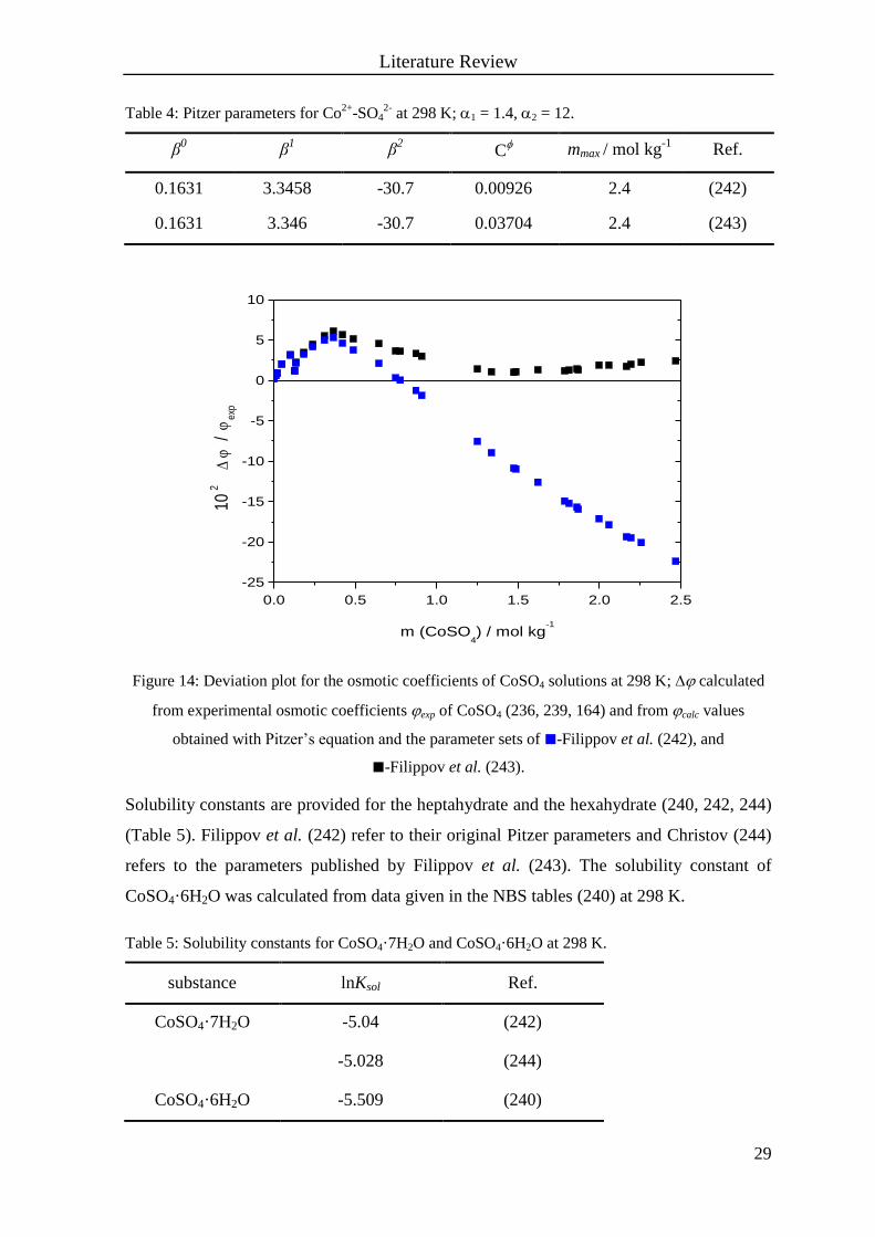
In the system Co2+
/ SO42-
// H2O, only two parameter sets that fulfill the requirement of
validity up to high concentrations are found in the literature (242, 243).
Filippov et al. (243) changed their parameters, while adjusting only C of their former set
(242). Nevertheless, the plot in Figure 14 reveals systematic deviations from experimental
data of up to 6%.
Literature Review
29
Table 4: Pitzer parameters for Co2+
-SO42-
at 298 K; 1 = 1.4, 2 = 12.
β0
β1 β
2 C
mmax / mol kg-1
Ref.
0.1631 3.3458 -30.7 0.00926 2.4 (242)
0.1631 3.346 -30.7 0.03704 2.4 (243)
0.0 0.5 1.0 1.5 2.0 2.5
-25
-20
-15
-10
-5
0
5
10
102
/
exp
m (CoSO4) / mol kg
-1
Figure 14: Deviation plot for the osmotic coefficients of CoSO4 solutions at 298 K; calculated
from experimental osmotic coefficients exp of CoSO4 (236, 239, 164) and from calc values
obtained with Pitzer’s equation and the parameter sets of -Filippov et al. (242), and
-Filippov et al. (243).
Solubility constants are provided for the heptahydrate and the hexahydrate (240, 242, 244)
(Table 5). Filippov et al. (242) refer to their original Pitzer parameters and Christov (244)
refers to the parameters published by Filippov et al. (243). The solubility constant of
CoSO4·6H2O was calculated from data given in the NBS tables (240) at 298 K.
Table 5: Solubility constants for CoSO4·7H2O and CoSO4·6H2O at 298 K.
substance lnKsol Ref.
CoSO4·7H2O -5.04 (242)
-5.028 (244)
CoSO4·6H2O -5.509 (240)

Literature Review
30
Three Pitzer parameter sets are published for the system Ni2+
/ SO42-
// H2O that are valid
up to high concentrations (Table 6).
Calculations of the deviations from experimental osmotic coefficients show that the
parameters of El Guendouzi et al. (233) account for the data (233, 234, 236-239) with
smallest deviations at high concentrations.
Table 6: Pitzer parameters for Ni2+
-SO42-
at 298 K; 1 = 1.4, 2 = 12.
β0
β1 β
2 C
mmax / mol kg-1
Ref.
0.1702 2.907 -40.06 0.0366 2.5 (230)
0.15471 3.0769 -37.593 0.04301 2.5 (232)
0.1625 2.903 -51.54 0.0389 2.5 (233)
Solubility constants for NiSO4·7H2O (35, 245) are provided in terms of the parameters of
Pitzer et al. (230). The solubility constant for -NiSO4·6H2O can be calculated from the
standard Gibbs energy of formation of the mineral, the ions Ni2+
, SO42-
and of water as
given in the NBS tables (240) at 298 K. The solubility constants mentioned are
summarized in Table 7.
0.0 0.5 1.0 1.5 2.0 2.5
-3
-2
-1
0
1
2
3
4
102
/
exp
m (NiSO4) / mol kg
-1
Figure 15: Deviation plot for the osmotic coefficients of NiSO4 solutions at 298 K; calculated
from experimental osmotic coefficients exp of NiSO4 (233, 234, 236-239) and from calc values
obtained with Pitzer’s equation and the parameter sets of -El Guendouzi et al. (233),
-Pitzer et al. (230), and -Kim et al. (232).
Literature Review
31
Table 7: Solubility constants for NiSO4·7H2O and -NiSO4·6H2O at 298 K.
substance lnKsol Ref.
NiSO4·7H2O 5.07 (35)
5.08 (245)
-NiSO4·6H2O -4.722 (240)
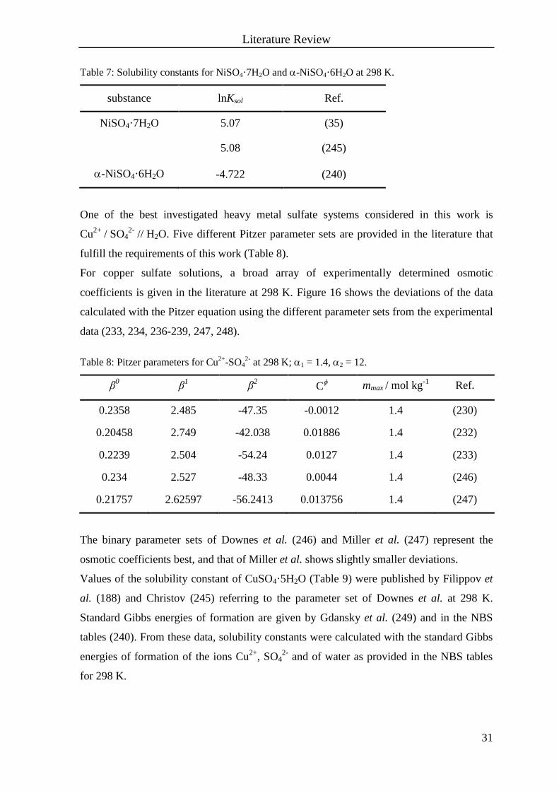
One of the best investigated heavy metal sulfate systems considered in this work is
Cu2+
/ SO42-
// H2O. Five different Pitzer parameter sets are provided in the literature that
fulfill the requirements of this work (Table 8).
For copper sulfate solutions, a broad array of experimentally determined osmotic
coefficients is given in the literature at 298 K. Figure 16 shows the deviations of the data
calculated with the Pitzer equation using the different parameter sets from the experimental
data (233, 234, 236-239, 247, 248).
Table 8: Pitzer parameters for Cu2+
-SO42-
at 298 K; 1 = 1.4, 2 = 12.
β0
β1 β
2 C
mmax / mol kg-1
Ref.
0.2358 2.485 -47.35 -0.0012 1.4 (230)
0.20458 2.749 -42.038 0.01886 1.4 (232)
0.2239 2.504 -54.24 0.0127 1.4 (233)
0.234 2.527 -48.33 0.0044 1.4 (246)
0.21757 2.62597 -56.2413 0.013756 1.4 (247)
The binary parameter sets of Downes et al. (246) and Miller et al. (247) represent the
osmotic coefficients best, and that of Miller et al. shows slightly smaller deviations.
Values of the solubility constant of CuSO4·5H2O (Table 9) were published by Filippov et
al. (188) and Christov (245) referring to the parameter set of Downes et al. at 298 K.
Standard Gibbs energies of formation are given by Gdansky et al. (249) and in the NBS
tables (240). From these data, solubility constants were calculated with the standard Gibbs
energies of formation of the ions Cu2+
, SO42-
and of water as provided in the NBS tables
for 298 K.
Literature Review
32
0.0 0.2 0.4 0.6 0.8 1.0 1.2 1.4 1.6 1.8
-3
-2
-1
0
1
2
3
102
/
exp
m (CuSO4) / mol kg
-1
Figure 16: Deviation plot for the osmotic coefficients of CuSO4 solutions at 298 K; calculated
from experimental osmotic coefficients exp of CuSO4 (233, 234, 236-239, 247, 248) and from calc
values obtained with Pitzer’s equation and the parameter sets of -Miller et al. (247), -Downes
et al. (246), -Pitzer et al. (230), -Kim et al. (232), and -El Guendouzi et al. (233).
Table 9: Solubility constants for CuSO4·5H2O at 298 K.
substance lnKsol Ref.
CuSO4·5H2O -6.06 (188)
-6.01 (245)
-6.63 (249)
-6.075 (240)
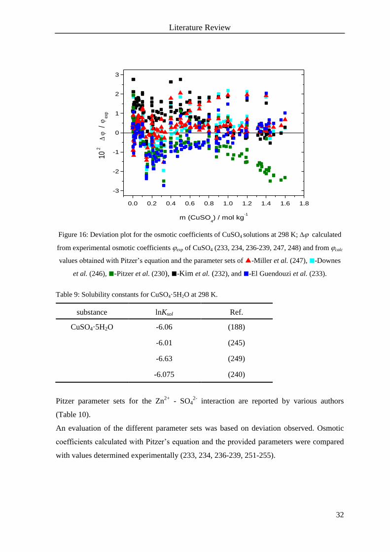
Pitzer parameter sets for the Zn2+
- SO42-
interaction are reported by various authors
(Table 10).
An evaluation of the different parameter sets was based on deviation observed. Osmotic
coefficients calculated with Pitzer’s equation and the provided parameters were compared
with values determined experimentally (233, 234, 236-239, 251-255).
Literature Review
33
Table 10: Pitzer parameters for Zn2+
-SO42-
at 298 K; 1 = 1.4, 2 = 12.
β0
β1 β
2 C
mmax / mol kg-1
Ref.
0.1949 2.883 -32.81 0.0299 3.5 (230)
0.18404 3.031 -27.709 0.03286 3.5 (232)
0.2224 2.671 -38.36 0.0182 3.5 (233)
0.1849 2.9614 -55.8433 0.0324 3.5 (250)
0.0 0.5 1.0 1.5 2.0 2.5 3.0 3.5 4.0 4.5
-10
-8
-6
-4
-2
0
2
4
6
102
/
m (ZnSO4) / mol kg
-1
Figure 17: Deviation plot for the osmotic coefficients of ZnSO4 solutions at 298 K; calculated
from experimental osmotic coefficients exp of ZnSO4 (233, 234, 236-239, 251-255) and from calc
values obtained with Pitzer’s equation and the parameter sets of -Mönig et al. (250), -Pitzer et
al. (230), -Kim et al. (232), and -El Guendouzi et al. (233).
From Figure 17, it can be seen, that the parameter set of Mönig et al. (250) characterizes
the experimental data with the least deviation.
Mönig et al. also calculated solubility constants for ZnSO4·7H2O, ZnSO4·6H2O and
ZnSO4·H2O. Another solubility constant for ZnSO4·7H2O was given by Filippov et al.
(206) which is consistent with the parameters of Pitzer et al. (230). Data for ZnSO4·6H2O
can be derived also from the NBS tables (240). The solubility constants are summarized in
Table 11.

Literature Review
34
Table 11: Solubility constants for ZnSO4·7H2O and ZnSO4·6H2O at 298 K.
substance lnKsol Ref.
ZnSO4·7H2O -4.285 (206)
-4.421 (250)
ZnSO4·6H2O -3.365 (250)
-4.065 (240)
Temperature-Dependence of the Ion Interaction Parameters for MSO4
(M = Mn, Co, Ni, Cu, Zn)
In order to describe the solubility at ambient temperatures, it is necessary to have
information on the temperature-dependence of the ion interaction parameters. This can be
obtained from experimental data for osmotic coefficients and activity coefficients at
different temperatures, and also from enthalpy or heat capacity data for the solutions.
The Thereda database (223) provides temperature functions of Pitzer parameters and Ksol
for the system Na+, K
+, Mg
2+, Ca
2+ / Cl
-, SO4
2- // H2O.
Activity coefficients at higher temperatures are published only for the systems
Cu2+
/ SO42-
// H2O (256, 257) and Zn2+
/ SO42-
// H2O (258, 259). The data consist of not
more than five data points per temperature, and were determined only in dilute solutions.
Heat capacity data for concentrated MSO4 (M = Mn, Co, Ni, Cu, Zn) solutions are not
provided in the literature.
However, relative apparent molar enthalpies of MSO4 solutions also make it possible to
determine the temperature-dependence of the ion interaction Pitzer parameters
(section 3.2.1.1). Königsberger et al. (260) demonstrated that data up to high
concentrations are needed to obtain enthalpy Pitzer parameters that result in a proper
prediction of solubility.
Different binary enthalpy parameters can be found for the required systems (Table 12),
although only the parameters of Königsberger et al. are valid at high concentrations.
Literature Review
35
Table 12: Enthalpy Pitzer parameters for M2+
-SO42-
at 298 K; 1 = 1.4, 2 = 12.
M 103
L(0)
102
L(1) 10
1 L(2)
103
CL
mmax / mol kg-1
Ref.
Mn 1.089
0 0 -0.318
1.5 (261)
Co 0.578
0.00648
0 -0.1268
1.4 (261)
Ni 0.75
0.0058
0 -0.1096
1.3 (261)
Cu -4.4
2.3
-4.7
1.2
1 (262)
Zn -3.6
2.3
-3.3
0.90
1 (262)
0.67
1.297
3.15
1.848
saturation (260)
Relative apparent molar enthalpies can be calculated from heats of dilution or heats of
dissolution, but only scarce data for either are available in the literature. Furthermore, all
data found were determined at 298 K. Riederer (263) measured heats of dilution at low
concentrations of MSO4 (M = Mg, Mn, Co, Ni, Zn), with less than 0.009 molal. Heats of
dilution at higher concentrations were determined by Schreiber et al. (261) for the heavy
metal sulfates MnSO4, CoSO4, and NiSO4. Stock solutions of around 1.7 molal were
diluted to concentrations ranging from 0.2 to 1.5 molal.
Soloveva et al. (264) calculated relative apparent molar enthalpies from dilution
measurements of nickel sulfate solutions in the concentration range from
0.278 to 2.40 molal. Heats of dissolution of NiSO4·6H2O were measured by Goldberg et
al. (265) in a small concentration range from 0.01 to 0.05 molal. Since the data of
Soloveva et al. and Goldberg et al. are published in molar terms, they had to be converted
in to units of mol kg-1
using the densities of NiSO4 solutions given by Söhnel et al. (266).
Heats of dilution of CuSO4 solutions were measured by Lange et al. (267). From these data
they calculated relative apparent molar enthalpies in the concentration range from
0.0001 to 1 molal.
There is a series of different data for zinc sulfate solutions. Lange et al. (267) calculated
relative apparent molar enthalpies in the concentration range from 0.0001 to 1 molal from
measured heats of dilution. A data set of relative partial molar heat contents is given by
Giauque et al. (268) over a concentration range from 1.01 to 3.58 molal. The values were
calculated from determined heats of dilution. From electromotive force measurements at
temperatures from 273 K to 323 K, Cowperthwaite et al. (258) calculated relative partial
molar enthalpies. Since discrepancies between the data of Lange et al. and Cowperthwaite
et al. were apparent, Harned (269) recalculated the data of Cowperthwaite et al., using a
Literature Review
36
quadratic equation rather than an equation with temperature to the fourth power. He also
evaluated the data again, and noted that the results at 323 K were inconsistent with those at
lower temperatures.
In the NBS tables (240) standard enthalpies of formation are given for different
concentrated solutions of the required sulfates MSO4 (M = Mn, Co, Ni, Cu, Zn) at 298 K.
3.3.2. Ternary Systems K+, M
2+ / SO4
2- // H2O
(M = Ca, Mg, Mn, Co, Ni, Cu, Zn)
3.3.2.1. Solubility Diagrams
Investigations of the above systems are largely confined to K+, M
2+ / SO4
2- // H2O
(M = Ca, Mg) at ambient temperatures.
Due to the low solubility of calcium sulfate, the solubility diagram for the system
K+, Ca
2+ / SO4
2- // H2O (Figure 18) differs considerably from those of other bivalent metal
systems. This is indicated by the completely different compositions and crystal structures
of the double salts syngenite (K2SO4·CaSO4·H2O) and görgeyite (K2SO4·5CaSO4·H2O), as
compared to the double salts formed by magnesium and the heavy metals with potassium
sulfate. Syngenite is stable in its aqueous solutions throughout the examined temperature
range from 298 K to 373 K (16, 17, 20, 31, 52, 270-272), although its stability field is
reduced continuously by görgeyite with increasing temperatures above 308 K.
For the system K+, Mg
2+ / SO4
2- // H2O, various studies are available at different
temperatures (15-18, 26-31, 37, 2-285). Depending on the temperature, the double salts
picromerite (K2SO4·MgSO4·6H2O), leonite (K2SO4·MgSO4·4H2O) and langbeinite
(K2SO4·2MgSO4) occur (Figure 19). Below 314 K, picromerite is the only stable double
salt in this system. At 320.65 K, the double salt crystallization branch consists entirely of
leonite (Figure 19). Thus, within the small interval of 6.5 K, leonite displaces picromerite.
Only one data point at 318 K is reported, where picromerite and leonite coexist (2),
although no experimental details concerning their determination were reported.

Literature Review
37
0.0 0.2 0.4 0.6 0.8 1.0 1.2
0.0
0.2
0.4
0.6
0.8
1.0
1.2
1.4
1.6
K2SO
4
CaSO4
H2O
CaSO4
K2SO
4
5CaSO4
H2O
CaSO4
2H2O
K2SO
4
m (
CaS
O4)
/ mol
kg
-1
m (K2SO
4) / mol kg
-1
Figure 18: Solubility diagram of the system K+, Ca
2+ / SO4
2- // H2O; -Cameron et al. (271)
at 298 K, -Hill (20) at 313 K, -Bodaleva et al. (17) at 328 K; -two-salt points;
curves-estimated solubility lines drawn by eye.
260 280 300 320 340 360 380
0.5
0.6
0.7
0.8
0.9
1.0
K2 SO
2MgSO
4
K2 SO
4
MgSO
4
4H2 O
K2SO
4
MgSO4
6H2O
K2SO
4
MgSO4
H2O
MgSO4
6H2O
MgSO4
7H2O
MgSO4
11H2O
Ice
x (M
gSO
4)
T / K
Figure 19: Polythermal solid-liquid equilibrium diagram of the system K+, Mg
2+ / SO4
2- // H2O;
x = mole fraction of MgSO4 of the anhydrous salt mixture; -D’Ans (2) at 318 K; -three-salt
points Jänecke (282); -three-salt points D’Ans (2); -(15-18, 26-31, 37, 2-285); curves-estimated
solubility lines drawn by eye.

Literature Review
38
As mentioned above, the data for the other remaining systems are less than satisfactory.
For the system K+, Mn
2+ / SO4
2- // H2O, an uncertainty with respect to the solid phases
formed at ambient temperatures is evident after an extensive search for solubility data in
the temperature range from 273 K to 373 K (21, 23, 25, 43, 46, 49, 138, 286, 287). Most of
the published values are two salt points. These data were determined mainly by Benrath et
al. (21) and combined in a polythermal diagram (Figure 20).
270 285 300 315 330 345 360 375
0.0
0.1
0.2
0.3
0.4
0.5
0.6
0.7
0.8
0.9
1.0
MnSO4
H2OMnSO
4
5H2O
K2 SO
4
MnSO
2H2 O
K2SO
4
2MnSO4
K2SO
4
MnSO4
7H2O
K2SO
4
MnSO4 4H
2O
x (M
nSO
4)
T / K
Figure 20: Polythermal solid-liquid equilibrium diagram for the system K+, Mn
2+ / SO4
2- // H2O;
x = mole fraction of MnSO4 of the anhydrous salt mixture; -Benrath (21),
-Caven et al. (23, 25); curves-estimated solubility lines drawn by eye.
From the diagram, he concluded that K2SO4·MnSO4·4H2O is stable up to 313 K and is
replaced by K2SO4·MnSO4·2H2O above this temperature. At high manganese sulfate
concentrations, K2SO4·2MnSO4 forms at temperatures above 298 K, adjacent to
K2SO4·MnSO4·4H2O and K2SO4·MnSO4·2H2O, respectively. With increasing
temperature, K2SO4·2MnSO4 displaces K2SO4·MnSO4·4H2O and K2SO4·MnSO4·2H2O.
Recent determinations of solubility by Hidalgo et al. (43) showed the formation of another
solid phase, K2SO4·3MnSO4·5H2O, at 308 K. The composition of the solid was confirmed
by a crystal structure analysis (43). In the literature another solid (K2SO4·MnSO4·1.5H2O)
is mentioned (288), but this is not figured in Benrath’s polythermal diagram.

Literature Review
39
In the four systems K+, M
2+ / SO4
2- // H2O (M = Co, Ni, Cu, Zn), the only double salt that
forms is K2SO4·MSO4·6H2O, over the temperature range from 273 K to 373 K. Ample
studies of the solubility were performed at 298 K. At higher temperatures, only scarce data
are provided, as summarized in Table 13.
Table 13: Literature sources on solubility in the systems in K+, M
2+ / SO4
2- // H2O
(M = Co, Ni, Cu, Zn).
M T / K Data Data points Reference
Co 273, 298, 311, 323,
348, 373 isotherms 100 (33, 35, 41, 42, 289-291)
273-373 two-salt points 57 (34, 42, 290-294)
Ni 293, 298, 318 isotherms 73 (23, 35, 44)
273-373 two-salt points 11 (290)
Cu 298, 308, 313, 324,
334 isotherms 33 (24, 19)
Zn 298, 308, 353, 373 isotherms 86 (21, 23, 36, 38, 45, 295)
273-343 two-salt points 26 (21, 205)
As can be seen from Table 13, the system K+, Co
2+ / SO4
2- // H2O is the one of the four
systems best described in the literature. Caven et al. (33) and Filippov et al. (41) performed
isothermal investigations at 298 K. At high concentrations of cobalt sulfate, the data sets
differ slightly from each other. Some years later, Filippov et al. (35) discussed his
experimental results again, giving data points calculated with Pitzer’s equation; these
resemble the data of Caven et al. more than those in his original experiments (Figure 21).
Caven et al. (23) and Filippov et al. (35) also provided data for the system
K+, Ni
2+ / SO4
2- // H2O at 298 K. However the data points of Caven et al. at 298 K were
excluded by Benrath (290), who performed polythermal investigations in the system.

Literature Review
40
0.0 0.2 0.4 0.6 0.8
0.0
0.5
1.0
1.5
2.0
2.5
3.0
CoSO4
7H2O
K2SO
4
K2SO
4
CoSO4
6H2O
m (
CoS
O4)
/ mol
kg
-1
m (K2SO
4) / mol kg
-1
Figure 21: Solubility diagram for the system K+, Co
2+ / SO4
2- // H2O at 298 K;
-Filippov et al. (41); -Caven et al. (33); -Filippov et al. (35); -two-salt point;
curves-estimated solubility lines drawn by eye.
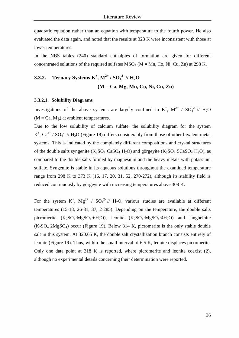
In the system K+, Zn
2+ / SO4
2- // H2O, four different data sets have been published for
298 K (23, 38, 45, 295). The crystallization branch of K2SO4·ZnSO4·6H2O for the two data
sets of Caven et al. (23) and D’Ans et al. (38), and of the data sets of Filippov et al. (45)
and Lipscomb et al. (295) agree with each other. At high concentrations of zinc sulfate,
differences in the data are noticeable. The data of D’Ans et al. and Caven et al. show a
stronger rise of the branch of K2SO4·ZnSO4·6H2O than those of Filippov et al. and
Lipscomb et al. (Figure 22). D’Ans et al. (38) determined data at 308 K. It is conspicuous
that their two-salt point for ZnSO4·7H2O-K2SO4·ZnSO4·6H2O at 298 K is almost at the
same concentration of potassium sulfate as the two-salt point at 308 K. From Figure 22, it
can also be seen that the slope of the K2SO4·ZnSO4·6H2O branch of D’Ans’s values at
308 K fits the data of Filippov et al. (45) and Lipscomb et al. (295). Further data at 308 K
were published by Shevchuk et al. (36), although they exhibit considerable scatter, and
therefore are not shown in Figure 22.
Literature Review
41
0.0 0.2 0.4 0.6 0.8 1.0
0
1
2
3
4
5
K2SO
4
ZnSO4
7H2O
K2SO
4
ZnSO4
6H2O
m (
ZnS
O4)
/ mol
kg
-1
m (K2SO
4) / mol kg
-1
Figure 22: Solubility diagram for the system K+, Zn
2+ / SO4
2- // H2O. At 298 K: -Filippov
et al. (45); -Lipscomb et al. (295); -D’Ans et al. (38), -Caven et al. (23); at 308 K:
-D’Ans et al. (38); -two-salt point; curves-estimated solubility lines drawn by eye.
3.3.2.2. Pitzer Mixing Parameters and Solubility Constants for Tutton’s Salts
Pitzer mixing parameters for the systems K+, M
2+ / SO4
2- // H2O (M = Ca, Mg) are
included in the Thereda data set (223), valid for the temperature range from 273 K to
393 K.
Pitzer mixing parameters for the heavy metal-containing systems K+, M
2+ / SO4
2- // H2O
(M = Co, Ni, Zn) were estimated by Filippov et al. (35, 45), but only at 298 K (Table 14).
Data at higher temperatures are not available. Solubility constants for the respective
Tutton’s salts are listed in Table 14, as given by different authors. Pitzer mixing parameters
and solubility constants for double salts in the system K+, Mn
2+ / SO4
2- // H2O have not
been published at any temperature.

Literature Review
42
Table 14: Pitzer mixing parameters for K-M-SO4 at 298 K and lnKsol of the respective Tutton’s
salts.
MK
4SOMK lnKsol (Tutton’s salts) Ref.
Co -0.127 0 -11.97 (35)
Ni -0.1419 0 -14.43 (35)
0 -0.069 -14.33 (244)
-0.01 -0.06114 -14.483 (296)
Cu -0.16 0.06 -13.26 (245)
Zn -0.0819 -0.0411 -12.66 (45)
-0.2 0.01 -13.401 (250)
3.3.3. Ternary Systems Ca2+
, M2+
/ SO42-
// H2O
(M = Mg, Mn, Co, Ni, Cu, Zn)
3.3.3.1. Solubility Diagrams
Few studies with scattered data exist concerning the solubility of gypsum and anhydrite,
respectively, in MSO4 solutions from low concentrations up to saturation of the metal
sulfate.
Umetsu et al. (297) examined the solubility of CaSO4 in solutions of zinc, magnesium,
copper, and cobalt sulfate over a temperature range of 298 K to 473 K. The data consist of
not more than five different metal sulfate concentrations at each temperature and are
published as mass concentrations (g L-1
). The values had to be converted into molalities
using the densities of Söhnel et al. (266).
For the system Mg2+
, Ca2+
/ SO42-
// H2O, several authors (17, 56, 62, 63, 70, 297-300)
have published data in the temperature range from 298 K to 328 K, although the majority
of the data deal with dilute solutions. Cameron et al. (298) and Kolosov (300) are the only
workers who determined the solubility of gypsum in magnesium sulfate solutions until
saturation with MgSO4·7H2O was achieved at 298 K. Data above 298 K were provided by
Novikova (56) at 308 K up to saturation of MgSO4·7H2O, and by Bodaleva et al. (17) at
328 K for gypsum and anhydrite up to 2.5 mol MgSO4/kg.
Table 15 summarizes the available data sources concerning the solubility of gypsum in
heavy metal sulfate solutions.

Literature Review
43
Table 15: Literature sources on the solubility of gypsum in M2+
/ SO42-
// H2O
(M = Mn, Co, Ni, Cu, Zn).
M T / K Molal concentration range m
mol kg-1
Data
points Reference
Mn 273 to 453 Dilute solutions to saturated MnSO4 89 (57)
298, 348 Dilute solutions to saturated MnSO4 23 (51)
303, 378 At 0.73 and 1.64 20 (82)
Co 298 to 473 From 0.5 to 0.7 40 (297)
Ni 318, 348, 363 From 0.4 to saturated NiSO4 43 (58)
Cu 298 to 473 From 0.8 to 1 43 (297)
298 Dilute solutions to 1.0 5 (62)
298, 318, 333 Dilute solutions to 1.0 18 (301)
Zn 298 to 473 From 0.15 to 1.3 53 (297)
298 Dilute solutions to 1.3 11 (302)
298, 318, 333 Dilute solutions to 1.7 21 (81)
3.3.3.2. Pitzer Mixing Parameters
Temperature-dependent Pitzer mixing parameters are not published for any of the ion
interactions in the systems Ca2+
, M2+
/ SO42-
// H2O (M = Mg, Mn, Co, Ni, Cu, Zn). At
298 K, mixing parameters are provided only for the systems Ca2+
, Mg2+
/ SO42-
// H2O by
Harvie et al. (225) ( 007.0MgCa , 024.04 SOMgCa ) and for Ca
2+, Zn
2+ / SO4
2- // H2O
by Mönig et al. (250) ( 0662.0ZnCa , 074.04 SOZnCa ).

Literature Review
44
3.3.4. Quaternary Systems K+, Ca
2+, M
2+ / SO4
2- // H2O
(M = Mg, Mn, Co, Ni, Cu, Zn)
3.3.4.1. Solubility Diagrams
The systems K+, Ca
2+, M
2+ / SO4
2- // H2O (M = Mg, Mn, Co, Ni, Cu, Zn) are the basic
systems in which polyhalite and its analogues appear. Solubility data are available only for
K+, Ca
2+, Mg
2+ / SO4
2- // H2O.
Initial investigations were performed by Basch (303), with an interest in the extension of
the crystallization field of polyhalite in this system at 298 K. Therefore, he determined the
three-salt points of polyhalite with adjacent solids (arcanite, epsomite, gypsum,
picromerite, syngenite, görgeyite). Later, van’t Hoff (1) published these results with other
data. Klooster (276) and Perova (304) carried out further studies at the same temperature
some years later, resulting in a larger stability field (Figure 23).
At 298 K, polyhalite has a small crystallization field, which expands with increasing
temperature. This is established by determinations of Lepeshkov et al. (16) at 308 K,
Bodaleva et al. (17) and Perova (31) at 328 K, Perova (31) at 348 K, and Conley et al.
(305) at 373 K. Above 373 K, data were provided by Dankiewicz et al. (306). The latter
data are not very reliable, because the solution was sampled after cooling in the presence of
the solid.
0.0 0.2 0.4 0.6 0.8 1.0 1.20.0 0.2 0.4 0.6 0.8 1.0 1.2
0.0
0.5
1.0
1.5
2.0
2.5
3.0
3.5
4.0
4.5
5.0
328 K
K2 SO
4 MgSO
4 2CaSO
4 2H
2 O
K2S
O4
MgSO4
6H2O
K2 SO
4 M
gSO4
4H2 O
K2SO
4
CaSO4
H2O
K2SO
4
5CaSO4
H2O
CaSO4
m (K2SO
4) / mol kg
-1
298 K
Ph
K2SO
4
K2SO
4
CaSO4
H2O
CaS
O4
2
H2O
K2 SO
4 M
gSO
4 6H
2 O
MgSO4
7H2O
m (
MgS
O4)
/ mol
kg
-1
m (K2SO
4) / mol kg
-1
Figure 23: Stability field of Mg-polyhalite in the system K+, Mg
2+, Ca
2+ / SO4
2- // H2O at 298K and
328 K; 298K: -Basch (303), van’t Hoff (1), -Klooster (276), -Perova (304),
-Cameron et al. 298 (16); 328 K: -Bodaleva et al. (17), -Perova (31); -three-salt point;
curves-estimated solubility lines drawn by eye.
Literature Review
45
3.3.4.2. Solubility Constant for Polyhalite and its Analogues
Harvie et al. (225) provided a chemical potential of polyhalite (/RT = -2282.5) at 298 K,
calculated from solubility data of Perova (304) and D’Ans (307) in the system
K+, Ca
2+, Mg
2+ / SO4
2- // H2O. However, D’Ans did not perform solubility experiments in
this system, but rather relied on data collected from the literature (1, 276)
At different temperatures between 273 K and 573 K, values of the solubility constant were
calculated by Risacher et al. (308). They based their calculations on the solubility constant
at 298 K and the temperature-dependence of the entropy of the formation reaction of the
corresponding mineral.
T
T
mR
T
T
mR
RmRRRmR
Rsolsol
RR
dTdT
TSd
RdT
dT
TSdT
RT
R
TS
T
T
R
TSTKTK
)(
303.2
1)(
303.2
1
303.2
)(
303.2
)()(lg)(lg
[48]
Here, TR denotes the reference temperature-298 K, and RS° the standard entropy of
reaction.
The required entropy of the formation reaction was calculated with
)()()( min,, TSTSTS mionmmR
[49]
where ionmS , refers to the standard molar entropy of an ion i, and
min,mS the standard molar
entropy of the corresponding mineral.
The standard entropies of the mineral at different temperatures were taken from the
literature. In the case of more complex and hydrated salts, the data were calculated from
tabulated entropies of simple anhydrous salts and the dehydration entropy of gypsum to
anhydrite. The solubility constants at 298 K were used as provided in the literature. For
Mg-polyhalite, the value of Harvie et al. (224) was employed.
Equilibrium investigations of Henneberg et al. (309) confirmed the calculated data of
Risacher et al. (308), especially at temperatures above 423 K.
There are no data for the heavy metal-containing polyhalites.
3.3.4.3. Enthalpy of Dissolution
Data for the enthalpy of dissolution of polyhalite and its analogues are not reported.
Richardson et al. (310) measured the effect of heat on the decomposition of polyhalite in
water.
Literature Review
46
3.3.5. Conclusions from the Literature Review
For modelling the crystallization fields of polyhalite and its analogues, the solubility
constants of these salts, as well as of the related solid phases (K2SO4, CaSO4·2H2O,
MSO4·xH2O, K2SO4·CaSO4·H2O, K2SO4·MSO4·xH2O, M = Mg, Mn, Co, Ni, Cu, Zn) are
required at 298 K. Therefore, not only the quaternary systems K+, Ca
2+, M
2+ / SO4
2- // H2O
but also the ternary systems K+, M
2+ / SO4
2- // H2O and Ca
2+, M
2+ / SO4
2- // H2O had to be
taken into account. Additionally, these systems are relevant for the evaluation and
determination of the required binary and mixing Pitzer parameters.
Since polyhalite forms slowly over months at 298 K, the solid-liquid phase equilibria
experiments had to be performed at 313 K. Hence, solubility data and modelling
parameters of the binary and ternary systems were required at 298 K and additionally at
313 K. Furthermore, enthalpies of dissolution are needed to extrapolate the solubility
constants from 313 K to 298 K.
Evaluation of the solubility data showed considerable deficiencies in the ternary systems.
For the systems Ca2+
, M2+
/ SO42-
// H2O (M = Mg, Mn, Co, Ni, Cu, Zn), almost no
solubility data are published for any temperature. Most of the systems
K+, M
2+ / SO4
2- // H2O are described well at 298 K, but deficiencies at higher temperatures
are revealed. Solubility investigations of the heavy metal-containing polyhalites in the
corresponding quaternary systems have not been performed at all.
In order to improve this situation, investigations had to be performed in
the system K+, Mg
2+ / SO4
2- // H2O at 318 K,
the system K+, Mn
2+ / SO4
2- // H2O at 298 K and 313 K,
the systems K+, M
2+ / SO4
2- // H2O (M = Co, Ni, Cu, Zn) at 313 K,
the systems Ca2+
, M2+
/ SO42-
// H2O (M = Mg, Mn, Co, Ni, Cu, Zn) at 298 K and
313 K,
the systems K+, Ca
2+, M
2+ / SO4
2- // H2O (M = Mg, Mn, Co, Ni, Cu, Zn) at 313 K.
Because the solid-liquid phase equilibria investigations of the quaternary systems had to be
executed at 313 K, Pitzer parameters at this temperature as well as at 298 K were
necessary.
For the heavy metal sulfates, binary parameters are provided only at 298 K, and the same is
encountered for the mixing parameters of K+-M
2+-SO4
2-. In the case of CoSO4, even the
parameters at 298 K need reinvestigation. So far, the published interactions of
Ca2+
-M2+
-SO42-
(Mg, Zn) only refer to 298 K. For the other heavy metals, parameters
remain undetermined at any temperature.
Literature Review
47
Hence, the estimation of the Pitzer parameters had to be accomplished for
the binary interactions of M2+
-SO42+
(M = Mn, Co, Ni, Cu, Zn) from 283 K to
323 K, and the corresponding solubility constants of the occurring salts,
the mixing interactions K+-M
2+-SO4
2+ (M = Mn, Co, Ni, Cu, Zn) at 313 K and for
K+-Mn
2+-SO4
2+ also at 298 K, as well as the determination of the solubility
constants of the occurring double salts,
the mixing interactions Ca2+
-M2+
-SO42+
(M = Mg, Mn, Co, Ni, Cu, Zn) at 298 K
and 313 K.
To evaluate the literature data for the systems K+, Ca
2+, Mg
2+ / SO4
2- // H2O, dissolution
experiments were performed at 303 K.
Calorimetric experiments had to be executed to obtain the enthalpies of dissolution of
polyhalite and its analogues at infinite dilution, in order to be able to extrapolate the
solubility constant from 313 K to 298 K.
Determination of Solubility Equilibria in the Ternary and Quaternary Systems
48
4. Determination of Solubility Equilibria in the Ternary and
Quaternary Systems with K+, Ca
2+, M
2+ and SO4
2- in H2O
(M = Mg, Mn, Co, Ni, Cu, Zn)
4.1. General Experimental Procedures
For the phase equilibrium studies, different amounts of metal sulfate and deionized water
(Seralpur Pro 90 CN) were weighed into waterproof, tightly sealed bottles (50 mL)
assuring a liquid level of at least three-quarters of the bottle. The samples were then placed
in a thermostatted water bath at the appropriate temperature (type ED, Julabo Labortechnik
GmbH with 15 magnetic stirring drives, H + P Labortechnik AG) so that they were
covered by water. During equilibration, the solutions were stirred thoroughly with a
Teflon-covered magnetic follower for varying durations, depending on the system and the
temperature. The temperature uncertainty was ± 0.1 K.
After equilibration, stirring was stopped and the solid allowed to settle for at least 12 h,
when the solution became clear. The bottles were placed on a platform inside the
thermostat, so they could be opened and still kept at the equilibrium temperature. A frit
with a glass fiber membrane of 0.6 µm pore size (MN 85/70, Macherey & Nagel) was
lowered into the solution and a certain mass of clear solution was separated from the solid
for chemical analyses.
The solid from each sample was isolated by suction filtration, washed with 4-5 mL of 40 %
ethanol and 4-5 mL of 96 % ethanol, and air-dried. Subsequently, solid phases were
identified by Raman spectroscopy and powder X-ray diffraction.
4.2. Ternary Systems K+, M
2+ / SO4
2- // H2O
(M = Mg, Mn, Co, Ni, Cu, Zn)
4.2.1. Experimental Procedures - K+, M
2+ / SO4
2- // H2O
Examinations of the system K+, Mg
2+ / SO4
2- // H2O were performed at 318 K. The heavy
metal-containing systems were investigated at 313 K, and K+, Mn
2+ / SO4
2- // H2O
additionally at 298 K.

Determination of Solubility Equilibria in the Ternary and Quaternary Systems
49
The general experimental procedure is described in section 4.1. The solutions were
prepared by weighing different amounts of potassium sulfate, bivalent metal sulfate
hydrate and deionized water into bottles. In the case of the copper-containing system,
around 0.5 g of 65 % HNO3 (p.a. Fluka) was weighed additionally into the bottles to
prevent the formation of basic double salts.
If all salts were dissolved after 24 h, additional potassium sulfate and bivalent metal sulfate
was added. This was repeated until a solid formed that did not disappear during 24 h.
Equilibration times referred to started with the appearance of a solid phase. The system
K+, Mg
2+ / SO4
2- // H2O was equilibrated for up to 100 days but not less than 78 days at 318
K. The equilibration time in the system K+, Mn
2+ / SO4
2- // H2O was 100 days at 298 K and
up to 95 days but not less than 28 days at 313 K. The other heavy metal-containing systems
were equilibrated for up to 56 days but not less than 40 days.
4.2.2. Results - K+, M
2+ / SO4
2- // H2O (M = Mg, Mn, Co, Ni, Cu, Zn)
All numerical data obtained are listed in Appendix B – Experimental Results in Table 31 to
Table 38. The analytical error for potassium and nickel is within 1 to 1.5 % of the total
concentration. The results of the other metal ions (Mg, Mn, Co, Cu, Zn) have an analytical
error of 0.5 to 1% of the total concentration.
System K+, Mg
2+ / SO4
2- // H2O
Determined solubility data are plotted in Figure 24. At the temperature examined, the two
double salts picromerite and leonite crystallize. The solution composition at the point of
coexistence of leonite and picromerite is 0.618 molal K2SO4 and 3.030 molal of MgSO4.
The course of the crystallization branches fits the picture of isotherms published for other
temperatures. In Figure 25, available solubility data are plotted for temperatures between
308 K and 328 K. With the data of the present work, the border between picromerite and
leonite can be fixed more precisely.
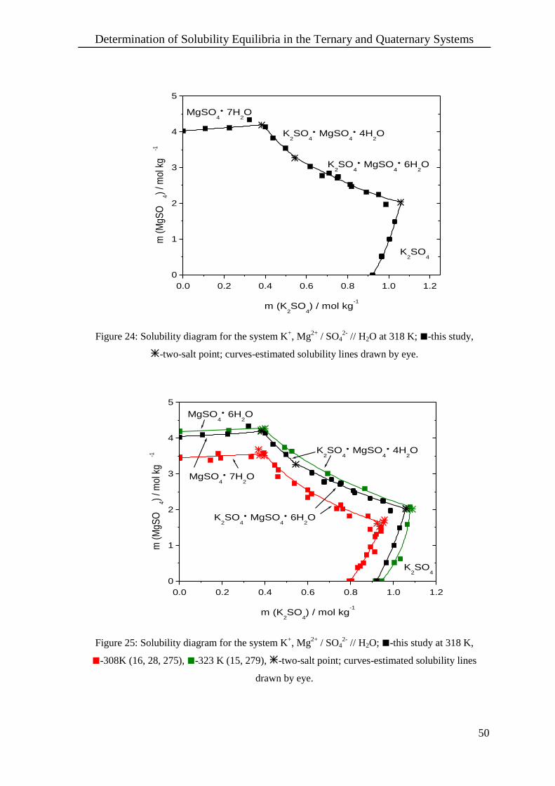
Determination of Solubility Equilibria in the Ternary and Quaternary Systems
50
0.0 0.2 0.4 0.6 0.8 1.0 1.2
0
1
2
3
4
5
K2SO
4
MgSO4
7H2O
K2SO
4
MgSO4
4H2O
K2SO
4
MgSO4
6H2O
m (
MgS
O4)
/ mol
kg
-1
m (K2SO
4) / mol kg
-1
Figure 24: Solubility diagram for the system K+, Mg
2+ / SO4
2- // H2O at 318 K; -this study,
-two-salt point; curves-estimated solubility lines drawn by eye.
0.0 0.2 0.4 0.6 0.8 1.0 1.2
0
1
2
3
4
5
MgSO4
6H2O
K2SO
4
MgSO4
6H2O
MgSO4
7H2O
K2SO
4
MgSO4
4H2O
K2SO
4
m (
MgS
O4)
/ mol
kg
-1
m (K2SO
4) / mol kg
-1
Figure 25: Solubility diagram for the system K+, Mg
2+ / SO4
2- // H2O; -this study at 318 K,
-308K (16, 28, 275), -323 K (15, 279), -two-salt point; curves-estimated solubility lines
drawn by eye.
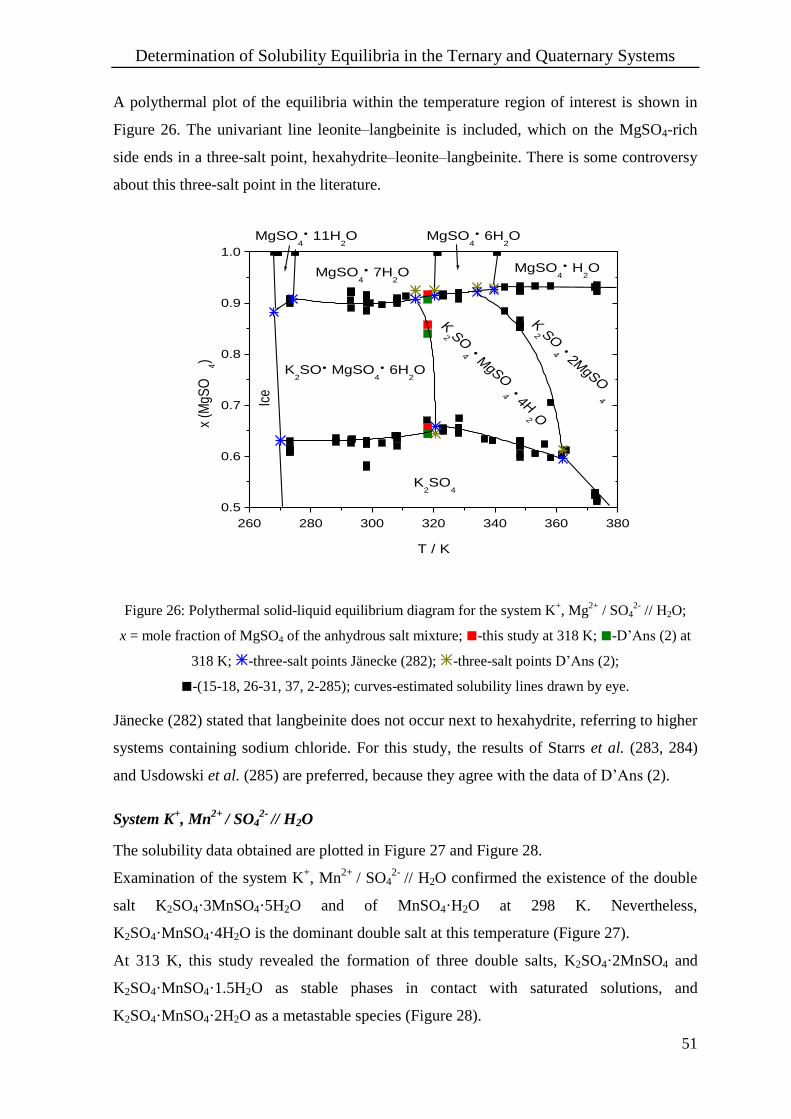
Determination of Solubility Equilibria in the Ternary and Quaternary Systems
51
A polythermal plot of the equilibria within the temperature region of interest is shown in
Figure 26. The univariant line leonite–langbeinite is included, which on the MgSO4-rich
side ends in a three-salt point, hexahydrite–leonite–langbeinite. There is some controversy
about this three-salt point in the literature.
260 280 300 320 340 360 380
0.5
0.6
0.7
0.8
0.9
1.0
K2 SO
4
2MgSO
4
K2 SO
4
MgSO
4
4H2 O
K2SO MgSO
4
6H2O
K2SO
4
MgSO4
H2O
MgSO4
6H2O
MgSO4
7H2O
MgSO4
11H2O
Ice
x (M
gSO
4)
T / K
Figure 26: Polythermal solid-liquid equilibrium diagram for the system K+, Mg
2+ / SO4
2- // H2O;
x = mole fraction of MgSO4 of the anhydrous salt mixture; -this study at 318 K; -D’Ans (2) at
318 K; -three-salt points Jänecke (282); -three-salt points D’Ans (2);
-(15-18, 26-31, 37, 2-285); curves-estimated solubility lines drawn by eye.
Jänecke (282) stated that langbeinite does not occur next to hexahydrite, referring to higher
systems containing sodium chloride. For this study, the results of Starrs et al. (283, 284)
and Usdowski et al. (285) are preferred, because they agree with the data of D’Ans (2).
System K+, Mn
2+ / SO4
2- // H2O
The solubility data obtained are plotted in Figure 27 and Figure 28.
Examination of the system K+, Mn
2+ / SO4
2- // H2O confirmed the existence of the double
salt K2SO4·3MnSO4·5H2O and of MnSO4·H2O at 298 K. Nevertheless,
K2SO4·MnSO4·4H2O is the dominant double salt at this temperature (Figure 27).
At 313 K, this study revealed the formation of three double salts, K2SO4·2MnSO4 and
K2SO4·MnSO4·1.5H2O as stable phases in contact with saturated solutions, and
K2SO4·MnSO4·2H2O as a metastable species (Figure 28).
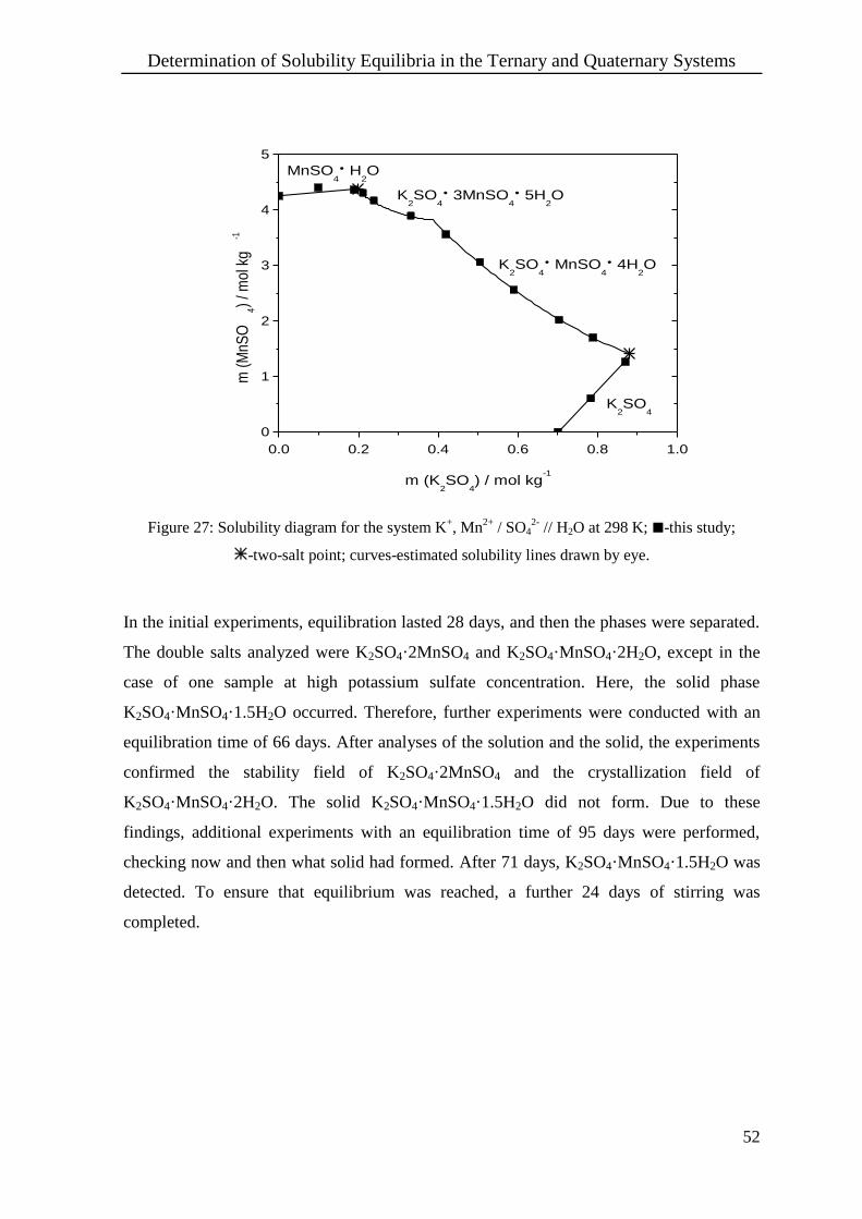
Determination of Solubility Equilibria in the Ternary and Quaternary Systems
52
0.0 0.2 0.4 0.6 0.8 1.0
0
1
2
3
4
5
K2SO
4
K2SO
4
MnSO4
4H2O
MnSO4
H2O
K2SO
4
3MnSO4
5H2O
m (
MnS
O4)
/ mol
kg
-1
m (K2SO
4) / mol kg
-1
Figure 27: Solubility diagram for the system K+, Mn
2+ / SO4
2- // H2O at 298 K; -this study;
-two-salt point; curves-estimated solubility lines drawn by eye.
In the initial experiments, equilibration lasted 28 days, and then the phases were separated.
The double salts analyzed were K2SO4·2MnSO4 and K2SO4·MnSO4·2H2O, except in the
case of one sample at high potassium sulfate concentration. Here, the solid phase
K2SO4·MnSO4·1.5H2O occurred. Therefore, further experiments were conducted with an
equilibration time of 66 days. After analyses of the solution and the solid, the experiments
confirmed the stability field of K2SO4·2MnSO4 and the crystallization field of
K2SO4·MnSO4·2H2O. The solid K2SO4·MnSO4·1.5H2O did not form. Due to these
findings, additional experiments with an equilibration time of 95 days were performed,
checking now and then what solid had formed. After 71 days, K2SO4·MnSO4·1.5H2O was
detected. To ensure that equilibrium was reached, a further 24 days of stirring was
completed.

Determination of Solubility Equilibria in the Ternary and Quaternary Systems
53
0.0 0.2 0.4 0.6 0.8 1.0 1.2
0
1
2
3
4
MnSO4
H2O
K2SO
4
MnSO4
1.5H2O
K2SO
4
2MnSO4
K2SO
4
MnSO4
2H2O
K2SO
4
m (
MnS
O4)
/ mol
kg
-1
m (K2SO
4) / mol kg
-1
Figure 28: Solubility diagram for the system K+, Mn
2+ / SO4
2- // H2O at 313 K; , -this study;
-two-salt point; curves-estimated solubility lines drawn by eye.
Solid-Liquid Equilibria at 298 K
In the earlier investigations of Caven et al. (23) and Dzhabarov et al. (286),
K2SO4·MnSO4·4H2O was found as the only double salt crystallizing at 298 K. The
solubility data determined by Dzhabarov et al. differ considerably from the data of Caven
et al. Unfortunately Dzhabarov et al. gave no experimental details.
Caven et al. (23) stirred the solutions for 3 days before analyzing them. From the present
study, it is known that an equilibration time of several weeks is needed. After four weeks,
the solid K2SO4·3MnSO4·5H2O occurred for the first time. A further eight weeks were
necessary to ensure equilibration. Caven et al. missed the formation of
K2SO4·3MnSO4·5H2O and found instead a larger stability field for MnSO4·4H2O and
K2SO·MnSO4·4H2O (Figure 29).
Caven et al. report the tetrahydrate as the stable manganese sulfate hydrate at 298 K,
whereas this study yields the monohydrate. For the binary system MnSO4-H2O
(section 3.3.1.1.) the penta-, tetra- or monohydrate was given as a stable phase at 298 K
according to different authors (113-139). The solubility curves of the various hydrates have
a crossing point near 298 K. Thus, solubility differences are small at this temperature and
consequently the transformation rate into the stable hydrate is slow. The results of this
study suggest that the monohydrate should be considered as the stable solid phase at
298 K.
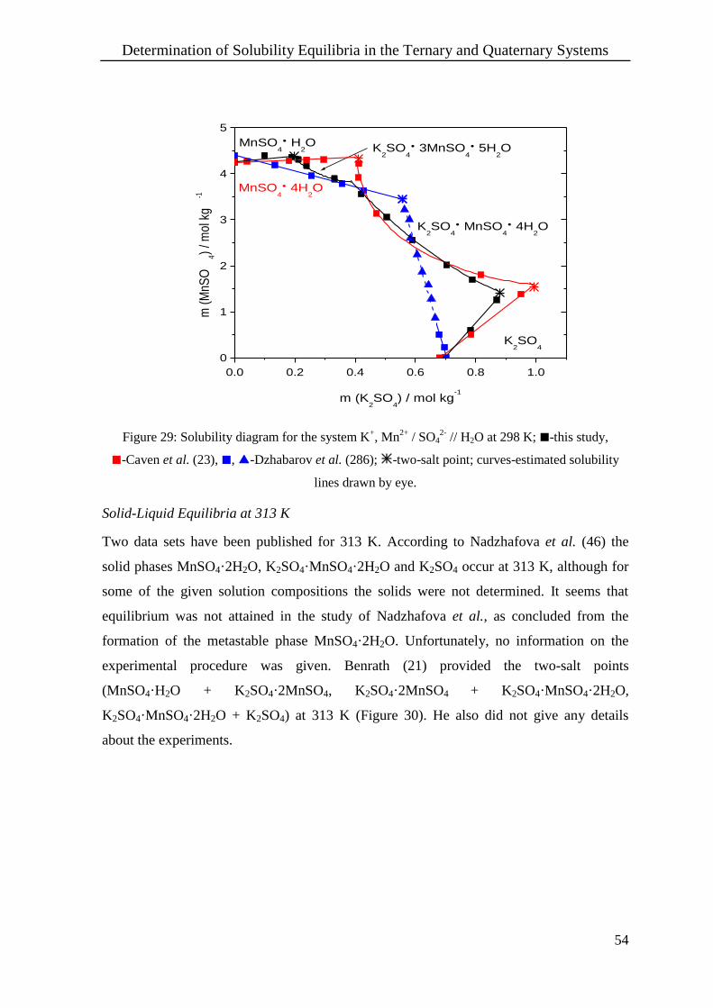
Determination of Solubility Equilibria in the Ternary and Quaternary Systems
54
0.0 0.2 0.4 0.6 0.8 1.0
0
1
2
3
4
5
MnSO4
4H2O
K2SO
4
K2SO
4
MnSO4
4H2O
MnSO4
H2O
K2SO
4
3MnSO4
5H2O
m (
MnS
O4)
/ mol
kg
-1
m (K2SO
4) / mol kg
-1
Figure 29: Solubility diagram for the system K+, Mn
2+ / SO4
2- // H2O at 298 K; -this study,
-Caven et al. (23), , -Dzhabarov et al. (286); -two-salt point; curves-estimated solubility
lines drawn by eye.
Solid-Liquid Equilibria at 313 K
Two data sets have been published for 313 K. According to Nadzhafova et al. (46) the
solid phases MnSO4·2H2O, K2SO4·MnSO4·2H2O and K2SO4 occur at 313 K, although for
some of the given solution compositions the solids were not determined. It seems that
equilibrium was not attained in the study of Nadzhafova et al., as concluded from the
formation of the metastable phase MnSO4·2H2O. Unfortunately, no information on the
experimental procedure was given. Benrath (21) provided the two-salt points
(MnSO4·H2O + K2SO4·2MnSO4, K2SO4·2MnSO4 + K2SO4·MnSO4·2H2O,
K2SO4·MnSO4·2H2O + K2SO4) at 313 K (Figure 30). He also did not give any details
about the experiments.
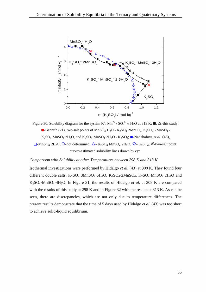
Determination of Solubility Equilibria in the Ternary and Quaternary Systems
55
0.0 0.2 0.4 0.6 0.8 1.0 1.2
0
1
2
3
4
MnSO4
H2O
K2SO
4
MnSO4
1.5H2O
K2SO
4
2MnSO4
K2SO
4
MnSO4
2H2O
K2SO
4
m (
MnS
O4)
/ mol
kg
-1
m (K2SO
4) / mol kg
-1
Figure 30: Solubility diagram for the system K+, Mn
2+ / SO4
2- // H2O at 313 K; , -this study;
-Benrath (21), two-salt points of MnSO4·H2O - K2SO4·2MnSO4, K2SO4·2MnSO4 -
K2SO4·MnSO4·2H2O, and K2SO4·MnSO4·2H2O - K2SO4; -Nadzhafova et al. (46),
-MnSO4·2H2O, -not determined, - K2SO4·MnSO4·2H2O, - K2SO4; -two-salt point;
curves-estimated solubility lines drawn by eye.
Comparison with Solubility at other Temperatures between 298 K and 313 K
Isothermal investigations were performed by Hidalgo et al. (43) at 308 K. They found four
different double salts, K2SO4·3MnSO4·5H2O, K2SO4·2MnSO4, K2SO4·MnSO4·2H2O and
K2SO4·MnSO4·4H2O. In Figure 31, the results of Hidalgo et al. at 308 K are compared
with the results of this study at 298 K and in Figure 32 with the results at 313 K. As can be
seen, there are discrepancies, which are not only due to temperature differences. The
present results demonstrate that the time of 5 days used by Hidalgo et al. (43) was too short
to achieve solid-liquid equilibrium.
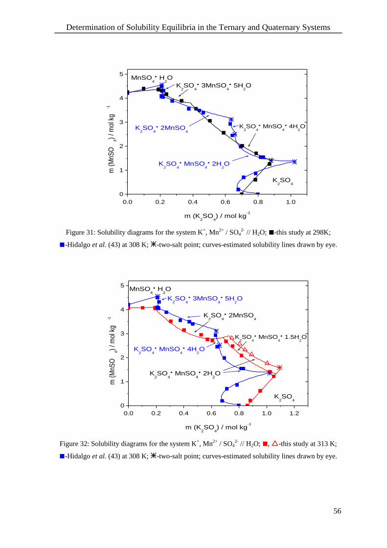
Determination of Solubility Equilibria in the Ternary and Quaternary Systems
56
0.0 0.2 0.4 0.6 0.8 1.0
0
1
2
3
4
5
K2SO
4
MnSO4
2H2O
K2SO
4
2MnSO4
K2SO
4
K2SO
4
MnSO4
4H2O
MnSO4
H2O
K2SO
4
3MnSO4
5H2O
m (
MnS
O4)
/ mol
kg
-1
m (K2SO
4) / mol kg
-1
Figure 31: Solubility diagrams for the system K+, Mn
2+ / SO4
2- // H2O; -this study at 298K;
-Hidalgo et al. (43) at 308 K; -two-salt point; curves-estimated solubility lines drawn by eye.
0.0 0.2 0.4 0.6 0.8 1.0 1.2
0
1
2
3
4
5
K2SO
4
MnSO4
1.5H2O
K2SO
4
3MnSO4
5H2O
MnSO4
H2O
K2SO
4
K2SO
4
MnSO4
4H2O
K2SO
4
MnSO4
2H2O
K2SO
4
2MnSO4
m (
MnS
O4)
/ mol
kg
-1
m (K2SO
4) / mol kg
-1
Figure 32: Solubility diagrams for the system K+, Mn
2+ / SO4
2- // H2O; , -this study at 313 K;
-Hidalgo et al. (43) at 308 K; -two-salt point; curves-estimated solubility lines drawn by eye.

Determination of Solubility Equilibria in the Ternary and Quaternary Systems
57
To summarize the results, the polythermal diagram as drawn by Benrath (21) has to be
modified (Figure 33).
The formation of the double salt K2SO4·3MnSO4·5H2O has to be considered at 298 K. Its
stability field should decrease with increasing temperature and disappearance is expected
near 310 K. Borene et al. (288) crystallized K2SO4·MnSO4·1.5H2O from equimolar
solutions at temperatures above 323 K. This study showed that K2SO4·MnSO4·1.5H2O
forms with a large stability field at 313 K. In considering these results, the question arises
as to whether K2SO4·MnSO4·2H2O is a stable double salt at all in this system.
270 285 300 315 330 345 360 375
0.0
0.1
0.2
0.3
0.4
0.5
0.6
0.7
0.8
0.9
1.0
K2SO
4
MnSO4
1.5H2O
K2SO
4
3MnSO4
5H2O
MnSO4
H2O
MnSO4
5H2O
K2 SO
4
MnSO
4
2H2 O
K2SO
4
2MnSO4
K2SO
4
MnSO4
7H2O
K2 SO
4
MnSO4
4H2 O
x (M
nSO
4)
T / K
Figure 33: Polythermal solubility diagram for the system K+, Mn
2+ / SO4
2- // H2O; -this study;
-Hidalgo et al. (43); -Benrath (21); -Caven et al. (23, 25); Borene et al. (288); estimated
solubility lines drawn by eye.
For the polythermal diagram, it is remarkable that the values of Hidalgo et al. and this
work give a smaller crystallization field for the manganese sulfate hydrates than
Benrath (21) and Caven et al. (23). As described above, Caven et al. missed the formation
of K2SO4·3MnSO4·5H2O, resulting in a larger branch of MnSO4·4H2O, and Benrath did
not give any details of his experimental procedure.
Compared with the other systems K+, M
2+ / SO4
2- // H2O (M = Mg, Co, Ni, Cu, Zn), the
system K+, Mn
2+ / SO4
2- // H2O requires much longer equilibration times. This might be due

Determination of Solubility Equilibria in the Ternary and Quaternary Systems
58
to the number of double salts (K2SO4·3MnSO4·5H2O, K2SO4·MnSO4·2H2O,
K2SO4·MnSO4·1.5H2O) forming only in this system.
System K+, M
2+ / SO4
2- // H2O (M = Co, Ni, Cu, Zn)
The results of the solubility experiments in the systems K+, M
2+ / SO4
2- // H2O
(M = Co, Ni, Cu, Zn) are plotted in Figure 34.
In all four systems, K2SO4·MSO4·6H2O, known as Tutton’s salt, is the only double salt
formed. The concentration range of the crystallization branch of Tutton’s salt varies with
the heavy metal ion. While K2SO4·NiSO4·6H2O forms from 0.04 molal to saturated NiSO4
solutions, the crystallization of K2SO4·CoSO4·6H2O requires concentrations above
0.4 molal CoSO4.
Figure 34: Solubility diagram for the system K+, M
2+ / SO4
2- // H2O (M = Co, Ni, Cu, Zn) at 313 K;
-this study, -two-salt point; curves-estimated solubility lines drawn by eye.
The system K+, Co
2+ / SO4
2- // H2O
Benrath (290) described the polytherm of the system in 1932, using his own determined
two-salt points and the isothermal data of Caven et al. (33). During investigations of the
reciprocal system KCl-CoSO4-H2O seven years later (289), it was noticed that his earlier
0
1
2
3
4
5
0.0 0.2 0.4 0.6 0.8 1.00.0 0.2 0.4 0.6 0.8 1.0
0
1
2
3
4
5
K2SO
4
K2SO
4
NiSO4
6H2O
-NiSO4
6H2O
K2SO
4
K2SO
4
CoSO4
6H2O
CoSO4
7H2O
m (
MS
O4)
(M =
Co,
Ni)
/ mol
kg
-1
K2SO
4
K2SO
4
ZnSO4
6H2O
ZnSO4
6H2O
m (K2SO
4) / mol kg
-1
K2SO
4
K2SO
4
CuSO4
6H2O
CuSO4
5H2O
m (
MS
O4)
(M =
Cu,
Zn)
/ m
ol k
g-1
m (K2SO
4) / mol kg
-1
0.4 0.5 0.6 0.7 0.8 0.9 1.00.00
0.05
0.10
0.15
K2SO
4
K2SO
4
NiSO4
6H2O

Determination of Solubility Equilibria in the Ternary and Quaternary Systems
59
polytherm was incorrect, especially at higher temperatures, but without referring to a
specific temperature. Thus, they examined the system again, determining isothermal
solubilities in the temperature range from 273 K to 372 K. Unfortunately, they did not give
any experimental details, even though he had pointed out the importance of the
equilibration times, which should extend for three days for solubility determinations at
higher temperatures. However, the data of Benrath et al. (290) are contradictory. At 323 K,
two two-salt points for CoSO4·6H2O-K2SO4·CoSO4·6H2O are given with considerably
different molalities of potassium sulfate (Figure 35). Furthermore, the more concentrated
potassium sulfate two-salt point for CoSO4·6H2O-K2SO4·CoSO4·6H2O and the two-salt
point of CoSO4·7H2O-K2SO4·CoSO4·6H2O are both at around 0.3 molal K2SO4 differing
only by the concentration of cobalt sulfate.
0.0 0.2 0.4 0.6 0.8 1.0 1.2
0.0
0.5
1.0
1.5
2.0
2.5
3.0
3.5
4.0
CoSO4
6H2O
K2SO
4
K2SO
4
CoSO4
6H2O
CoSO4
7H2O
m (
CoS
O4)
/ mol
kg
-1
m (K2SO
4) / mol kg
-1
Figure 35: Solubility diagram for the system K+, Co
2+ / SO4
2- // H2O; -this study at 313 K;
-(33,41) at 298 K; -Benrath et al. (289) at 311 K; -Benrath et al. (289) at 323 K; -two-salt
point; curves-estimated solubility lines drawn by eye.
A comparison of the data of this study with the values of Benrath et al. (289) determined at
311 K shows noticeable differences for highly concentrated cobalt sulfate solutions
(Figure 35). The crystallization branch of K2SO4·CoSO4·6H2O found here fits the pattern
of the isotherms at 298 K and at 323 K, and thus the Benrath data at 311 K must be partly
in error.

Determination of Solubility Equilibria in the Ternary and Quaternary Systems
60
The system K+, Ni
2+ / SO4
2- // H2O
In the system K+, Ni
2+ / SO4
2- // H2O, isothermal solubility data are published for 293 K,
298 K and 318 K (23, 35, 44).
As can be seen in Figure 36, the two-salt point for -NiSO4·6H2O-K2SO4·NiSO4·6H2O of
Benrath given for 313 K is at a noticeably higher molality of potassium sulfate than the
point found in this study. Regrettably, Benrath did not give any details on experimental
procedure. However, the data of Druzhinin et al. (44) determined at 318 K scatter
considerably and show a very strange form for the K2SO4·NiSO4·6H2O branch. The two-
salt point of -NiSO4·6H2O - K2SO4·NiSO4·6H2O was measured four times at 313 K with
only slight differences in concentrations. Furthermore, the values are provided for a
temperature only 5 K above the one of this study. For that reason, they should be of similar
concentration. Therefore, the two-salt point of Druzhinin et al. seems more precise than
that published by Benrath.
The course of the crystallization branch of K2SO4 fits the inclination of the isotherm at
298 K and 318 K. Here, contrary to the systems with MSO4 (M = Co, Cu, Zn), the
solubility of potassium sulfate decreases with increasing concentrations of nickel sulfate at
elevated temperatures.
Figure 36: Solubility diagram for the system K+, Ni
2+ / SO4
2- // H2O; -this study at 313 K;
-Filippov et al. (35) at 298 K; -Benrath et al. (290) at 311 K; -Druzhinin et al. (44) at 318 K;
-two-salt point; curves-estimated solubility lines drawn by eye.
0.0 0.1 0.2 0.3 0.4 0.5 0.6 0.7 0.8 0.9 1.0
0.0
0.5
1.0
1.5
2.0
2.5
3.0
3.5
NiS
O4
7
H2O
K2SO
4
K2SO
4
NiSO4
6H2O
-NiSO4
6H2O
m (
NiS
O4)
/ m
ol k
g-1
m (K2SO
4) / mol kg
-1
0.4 0.5 0.6 0.7 0.8 0.9 1.00.00
0.05
0.10
0.15
K2SO
4
K2SO
4
NiSO4
6H2O
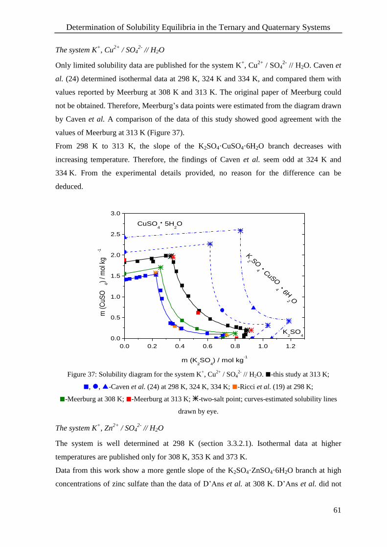
Determination of Solubility Equilibria in the Ternary and Quaternary Systems
61
The system K+, Cu
2+ / SO4
2- // H2O
Only limited solubility data are published for the system K+, Cu
2+ / SO4
2- // H2O. Caven et
al. (24) determined isothermal data at 298 K, 324 K and 334 K, and compared them with
values reported by Meerburg at 308 K and 313 K. The original paper of Meerburg could
not be obtained. Therefore, Meerburg’s data points were estimated from the diagram drawn
by Caven et al. A comparison of the data of this study showed good agreement with the
values of Meerburg at 313 K (Figure 37).
From 298 K to 313 K, the slope of the K2SO4·CuSO4·6H2O branch decreases with
increasing temperature. Therefore, the findings of Caven et al. seem odd at 324 K and
334 K. From the experimental details provided, no reason for the difference can be
deduced.
0.0 0.2 0.4 0.6 0.8 1.0 1.2
0.0
0.5
1.0
1.5
2.0
2.5
3.0
K2SO
4
K2 SO
4
CuSO
4
6H2 O
CuSO4
5H2O
m (
CuS
O4)
/ mol
kg
-1
m (K2SO
4) / mol kg
-1
Figure 37: Solubility diagram for the system K+, Cu
2+ / SO4
2- // H2O. -this study at 313 K;
, , -Caven et al. (24) at 298 K, 324 K, 334 K; -Ricci et al. (19) at 298 K;
-Meerburg at 308 K; -Meerburg at 313 K; -two-salt point; curves-estimated solubility lines
drawn by eye.
The system K+, Zn
2+ / SO4
2- // H2O
The system is well determined at 298 K (section 3.3.2.1). Isothermal data at higher
temperatures are published only for 308 K, 353 K and 373 K.
Data from this work show a more gentle slope of the K2SO4·ZnSO4·6H2O branch at high
concentrations of zinc sulfate than the data of D’Ans et al. at 308 K. D’Ans et al. did not

Determination of Solubility Equilibria in the Ternary and Quaternary Systems
62
give details about their equilibration times, only mentioning that times exceeding two days
are necessary. The two-salt point of Benrath is obviously in the region of supersaturation.
0.0 0.2 0.4 0.6 0.8 1.0
0
1
2
3
4
5
ZnS
O4
7
H2O
K2SO
4
ZnSO4
6H2O
K2SO
4
ZnSO4
6H2O
m (
ZnS
O4)
/ mol
kg
-1
m (K2SO
4) / mol kg
-1
Figure 38: Solubility diagram for the system K+, Zn
2+ / SO4
2- // H2O. -this study at 313 K;
-Filippov et al. (45), Lipscomb et al. (295) at 298 K; -D’Ans et al. (38) at 308 K; -Benrath
(21) at 313 K; -two-salt point; curves-estimated solubility lines drawn by eye.
4.3. Ternary Systems Ca2+
, M2+
/ SO42-
// H2O
(M = Mg, Mn, Co, Ni, Cu, Zn)
4.3.1. Experimental Procedures - Ca2+
, M2+
/ SO42-
// H2O
The systems Ca2+
, M2+
/ SO42-
// H2O (M = Mg, Mn, Co, Ni, Cu, Zn) were investigated at
298 K and 313 K. An additional isotherm at 333 K was established for the system
Ca2+
, Mg2+
/ SO42-
// H2O.
The general experimental procedure is described in section 4.1. The starting solutions were
obtained by weighing deionized water and appropriate amounts of the metal sulfate
hydrates into waterproof tightly sealed bottles.
The metal sulfate solution were kept at least 12 h in the thermostat at the desired
temperature, before adding CaSO4·0.5H2O to the solutions at 298 K and 313 K, or CaSO4
in the case of magnesium sulfate solutions at 333 K.
Samples at 298 K were equilibrated for up to 28 days but at least for 11 days. The 313 K
samples were stirred for up to 50 days but at least for 28 days to ensure that gypsum and

Determination of Solubility Equilibria in the Ternary and Quaternary Systems
63
not anhydrite was the stable phase, especially in concentrated MSO4 solutions. An
equilibration time of 22 days was used for the samples at 333 K.
4.3.2. Results - Ca2+
, M2+
/ SO42-
// H2O (M = Mg, Mn, Co, Ni, Cu, Zn)
The solubility data obtained are listed in Appendix B – Experimental Results in Table 39
to Table 45 and plotted in Figure 39 and Figure 40. For calcium, an analytical error of up
to 7 % of the total concentration is indicated. For Mg, Mn, Co, Ni, Cu and Zn, an error of
around 1 % of the total concentration is indicated for the two-salt points.
0.0
0.5
1.0
1.5
2.0
0.0
0.5
1.0
1.5
2.0
0 1 2 3 4
0.0
0.5
1.0
1.5
2.0
0 1 2 3 4
Mg
102 m
(C
aSO
4)
/ mol
kg
-1
Co
Mn
Ni
Cu
m (MSO4 (M = Mg, Mn, Co, Ni, Cu, Zn)) / mol kg
-1
Zn
Figure 39: Molal solubility of gypsum in MSO4 solutions (M = Mg, Mn, Co, Ni, Cu, Zn);
-at 298 K, - 313 K; -two-salt point; vertical lines indicate uncertainty
at the 95 % confidence limit; curves-estimated solubility lines drawn by eye.

Determination of Solubility Equilibria in the Ternary and Quaternary Systems
64
As can be seen for all ternary systems, the solubility of gypsum decreases at low
concentrations of bivalent metal sulfate until it reaches a minimum. Then it rises with
increasing amount of magnesium or heavy metal sulfate to a maximum. With further
increase of metal sulfate concentration, the gypsum solubility decreases again until
saturation of the added bivalent metal sulfate is reached. Over the whole concentration
range no double salt formation was observed. The form of the solubility curves is the same
at 298 K and at 313 K. In the system Ca2+
, Mn2+
/ SO42-
// H2O at 313 K, the minimum
gypsum solubility is distinguishably lower (1·10-2
molal CaSO4) than in the other systems
(1.3·10-2
molal CaSO4). From the diagrams, it can be seen that CaSO4·2H2O solubility
increases with temperature. The solubility of anhydrite shows the same dependence on the
concentration of magnesium sulfate in solution as does gypsum.
In Figure 41, the effect of the various sulfates on the solubility of gypsum is compared at
298 K.
0 1 2 3 4 5
0.0
0.2
0.4
0.6
0.8
1.0
1.2
1.4
1.6
1.8
MgSO4
. 6H2O
CaSO4
102 m
(C
aSO
4)
/ mol
kg
-1
m (MgSO4) / mol kg
-1
Figure 40: Molal solubility of anhydrite in MgSO4-H2O at 333 K; -this study; -two-salt point;
vertical lines indicate uncertainty at the 95 % confidence limit; curves-estimated solubility lines
drawn by eye.

Determination of Solubility Equilibria in the Ternary and Quaternary Systems
65
0.0 0.5 1.0 1.5 2.0 2.5 3.0 3.5 4.0 4.5
0.0
0.2
0.4
0.6
0.8
1.0
1.2
1.4
1.6
1.8
102 m
(C
aSO
4)
/ mol
kg
-1 H
2O
m (MSO4 M = Mg, Mn, Co, Ni, Cu, Zn) / mol kg
-1 H
2O
Figure 41: Molal solubility of gypsum in MSO4 + H2O (M = Mg, Mn, Co, Ni, Cu, Zn) at 298 K;
-Mg, -(Mn, Co, Ni, Cu, Zn); -two-salt point; vertical lines indicate uncertainty at the 95 %
confidence limit; curves-estimated solubility lines drawn by eye.
Systematic trends within the series MSO4 (M = Mn, Co, Ni, Cu, Zn) are difficult to
recognize (Figure 41). The results show that gypsum solubility in MgSO4 solutions is
lowest and well-distinguished from the other solutions. Systematic errors can be excluded.
The method chosen for the ICP-OES calcium analyses minimizes non-spectroscopic and
spectroscopic interferences as much as possible. In addition, the calcium wavelength used
for measurements shows no spectroscopic interference with any of the other elements
present in the samples, although the wavelength is slightly less sensitive.
System Ca2+
, Mg2+
/ SO42-
// H2O
From the literature (298, 56, 62), it is known that difficulties in the analyses of calcium in
concentrated bivalent metal sulfate solution appear. For this reason, most of the literature
data for the ternary system Ca2+
, Mg2+
/ SO42-
// H2O at 298 K refer to dilute solutions of
magnesium sulfate. In dilute solutions, the solubility curves of gypsum of all authors
coincide. For higher concentrations, only Cameron et al. (298) and Kolosov (300)
published data. Both differ slightly in the CaSO4 concentration at the minimum of the
curve but more at magnesium concentrations above 1.6 molal MgSO4. The experimental
data of this work resemble the results of Cameron et al. up to a MgSO4 concentration of
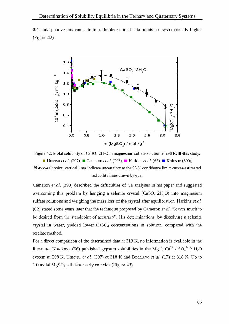
Determination of Solubility Equilibria in the Ternary and Quaternary Systems
66
0.4 molal; above this concentration, the determined data points are systematically higher
(Figure 42).
0.0 0.5 1.0 1.5 2.0 2.5 3.0 3.5
0.4
0.6
0.8
1.0
1.2
1.4
1.6
MgS
O4
7
H2O
CaSO4
2H2O
10
2 m
(C
aSO
4)
/ mol
kg
-1
m (MgSO4) / mol kg
-1
Figure 42: Molal solubility of CaSO4·2H2O in magnesium sulfate solution at 298 K; -this study,
-Umetsu et al. (297), -Cameron et al. (298), -Harkins et al. (62), -Kolosov (300);
-two-salt point; vertical lines indicate uncertainty at the 95 % confidence limit; curves-estimated
solubility lines drawn by eye.
Cameron et al. (298) described the difficulties of Ca analyses in his paper and suggested
overcoming this problem by hanging a selenite crystal (CaSO4·2H2O) into magnesium
sulfate solutions and weighing the mass loss of the crystal after equilibration. Harkins et al.
(62) stated some years later that the technique proposed by Cameron et al. “leaves much to
be desired from the standpoint of accuracy”. His determinations, by dissolving a selenite
crystal in water, yielded lower CaSO4 concentrations in solution, compared with the
oxalate method.
For a direct comparison of the determined data at 313 K, no information is available in the
literature. Novikova (56) published gypsum solubilities in the Mg2+
, Ca2+
/ SO42-
// H2O
system at 308 K, Umetsu et al. (297) at 318 K and Bodaleva et al. (17) at 318 K. Up to
1.0 molal MgSO4, all data nearly coincide (Figure 43).
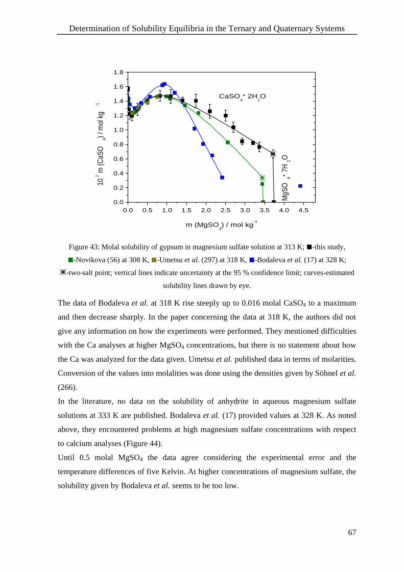
Determination of Solubility Equilibria in the Ternary and Quaternary Systems
67
0.0 0.5 1.0 1.5 2.0 2.5 3.0 3.5 4.0 4.5
0.0
0.2
0.4
0.6
0.8
1.0
1.2
1.4
1.6
1.8
MgS
O4
7
H2O
CaSO4
2H2O
102 m
(C
aSO
4)
/ mol
kg
-1
m (MgSO4) / mol kg
-1
Figure 43: Molal solubility of gypsum in magnesium sulfate solution at 313 K; -this study,
-Novikova (56) at 308 K, -Umetsu et al. (297) at 318 K, -Bodaleva et al. (17) at 328 K;
-two-salt point; vertical lines indicate uncertainty at the 95 % confidence limit; curves-estimated
solubility lines drawn by eye.
The data of Bodaleva et al. at 318 K rise steeply up to 0.016 molal CaSO4 to a maximum
and then decrease sharply. In the paper concerning the data at 318 K, the authors did not
give any information on how the experiments were performed. They mentioned difficulties
with the Ca analyses at higher MgSO4 concentrations, but there is no statement about how
the Ca was analyzed for the data given. Umetsu et al. published data in terms of molarities.
Conversion of the values into molalities was done using the densities given by Söhnel et al.
(266).
In the literature, no data on the solubility of anhydrite in aqueous magnesium sulfate
solutions at 333 K are published. Bodaleva et al. (17) provided values at 328 K. As noted
above, they encountered problems at high magnesium sulfate concentrations with respect
to calcium analyses (Figure 44).
Until 0.5 molal MgSO4 the data agree considering the experimental error and the
temperature differences of five Kelvin. At higher concentrations of magnesium sulfate, the
solubility given by Bodaleva et al. seems to be too low.
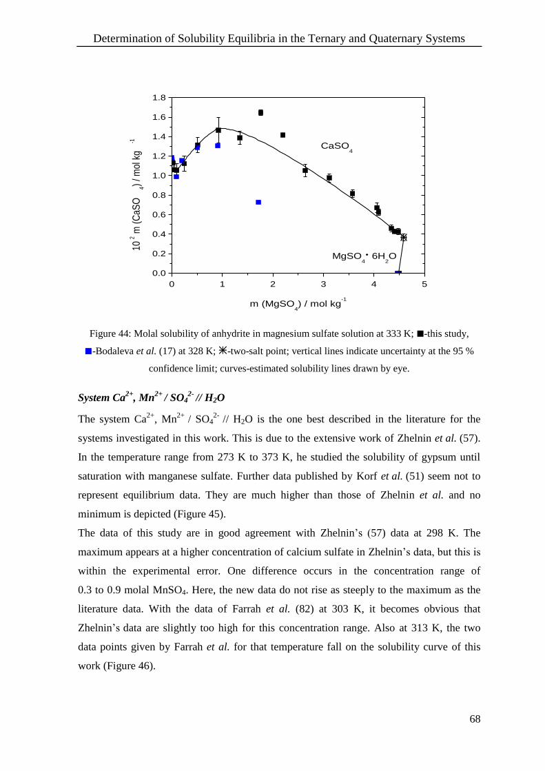
Determination of Solubility Equilibria in the Ternary and Quaternary Systems
68
0 1 2 3 4 5
0.0
0.2
0.4
0.6
0.8
1.0
1.2
1.4
1.6
1.8
MgSO4
6H2O
CaSO4
102 m
(C
aSO
4)
/ mol
kg
-1
m (MgSO4) / mol kg
-1
Figure 44: Molal solubility of anhydrite in magnesium sulfate solution at 333 K; -this study,
-Bodaleva et al. (17) at 328 K; -two-salt point; vertical lines indicate uncertainty at the 95 %
confidence limit; curves-estimated solubility lines drawn by eye.
System Ca2+
, Mn2+
/ SO42-
// H2O
The system Ca2+
, Mn2+
/ SO42-
// H2O is the one best described in the literature for the
systems investigated in this work. This is due to the extensive work of Zhelnin et al. (57).
In the temperature range from 273 K to 373 K, he studied the solubility of gypsum until
saturation with manganese sulfate. Further data published by Korf et al. (51) seem not to
represent equilibrium data. They are much higher than those of Zhelnin et al. and no
minimum is depicted (Figure 45).
The data of this study are in good agreement with Zhelnin’s (57) data at 298 K. The
maximum appears at a higher concentration of calcium sulfate in Zhelnin’s data, but this is
within the experimental error. One difference occurs in the concentration range of
0.3 to 0.9 molal MnSO4. Here, the new data do not rise as steeply to the maximum as the
literature data. With the data of Farrah et al. (82) at 303 K, it becomes obvious that
Zhelnin’s data are slightly too high for this concentration range. Also at 313 K, the two
data points given by Farrah et al. for that temperature fall on the solubility curve of this
work (Figure 46).

Determination of Solubility Equilibria in the Ternary and Quaternary Systems
69
0.0 0.5 1.0 1.5 2.0 2.5 3.0 3.5 4.0 4.5 5.0
0.0
0.4
0.8
1.2
1.6
2.0
2.4
2.8
MnS
O4
5
H2O
MnSO4
H2O
CaSO4
2H2O
102 m
(C
aSO
4)
/ mol
kg
-1
m (MnSO4) / mol kg
-1
Figure 45: Molal gypsum solubility in MnSO4 solution at 298 K; -this study, -Zhelnin et al.
(57), -Korf et al. (51), -Farrah et al. (82) at 303 K; -two-salt point; vertical lines indicate
uncertainty at the 95 % confidence limit; curves-estimated solubility lines drawn by eye.
0.0 0.5 1.0 1.5 2.0 2.5 3.0 3.5 4.0 4.5
0.0
0.2
0.4
0.6
0.8
1.0
1.2
1.4
1.6
1.8
2.0
MnS
O4
H
2O
CaSO4
2H2O
102 m
(C
aSO
4)
/ mol
kg
-1
m (MnSO4) / mol kg
-1
Figure 46: Molal gypsum solubility in MnSO4 solution at 313 K; -this study, -Zhelnin
et at. (57) at 323 K, -Farrah et al. (82) at 313 K; -two-salt point; vertical lines indicate
uncertainty at the 95 % confidence limit; curves-estimated solubility lines drawn by eye.
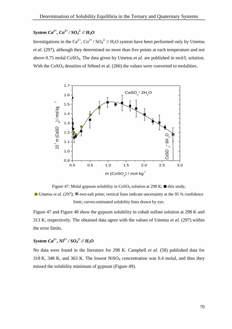
Determination of Solubility Equilibria in the Ternary and Quaternary Systems
70
System Ca2+
, Co2+
/ SO42-
// H2O
Investigations in the Ca2+
, Co2+
/ SO42-
// H2O system have been performed only by Umetsu
et al. (297), although they determined no more than five points at each temperature and not
above 0.75 molal CoSO4. The data given by Umetsu et al. are published in mol/L solution.
With the CoSO4 densities of Söhnel et al. (266) the values were converted to molalities.
0.0 0.5 1.0 1.5 2.0 2.5 3.0
0.9
1.0
1.1
1.2
1.3
1.4
1.5
1.6
1.7
CoS
O4
6
H2O
CaSO4
2H2O
102 m
(C
aSO
4)
/ mol
kg
-1
m (CoSO4) / mol kg
-1
Figure 47: Molal gypsum solubility in CoSO4 solution at 298 K; -this study,
-Umetsu et al. (297); -two-salt point; vertical lines indicate uncertainty at the 95 % confidence
limit; curves-estimated solubility lines drawn by eye.
Figure 47 and Figure 48 show the gypsum solubility in cobalt sulfate solution at 298 K and
313 K, respectively. The obtained data agree with the values of Umetsu et al. (297) within
the error limits.
System Ca2+
, Ni2+
/ SO42-
// H2O
No data were found in the literature for 298 K. Campbell et al. (58) published data for
318 K, 348 K, and 363 K. The lowest NiSO4 concentration was 0.4 molal, and thus they
missed the solubility minimum of gypsum (Figure 49).
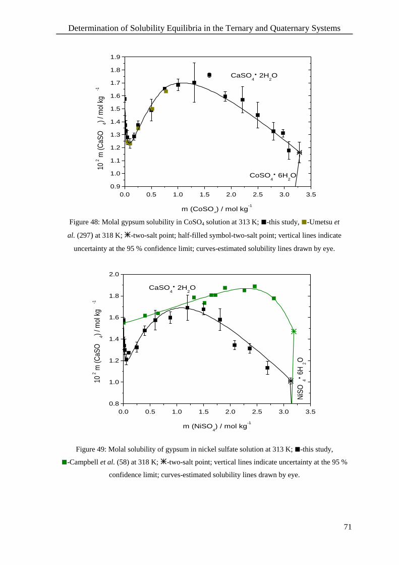
Determination of Solubility Equilibria in the Ternary and Quaternary Systems
71
0.0 0.5 1.0 1.5 2.0 2.5 3.0 3.5
0.9
1.0
1.1
1.2
1.3
1.4
1.5
1.6
1.7
1.8
1.9
CoSO4
6H2O
CaSO4
2H2O
102 m
(C
aSO
4)
/ mol
kg
-1
m (CoSO4) / mol kg
-1
Figure 48: Molal gypsum solubility in CoSO4 solution at 313 K; -this study, -Umetsu et
al. (297) at 318 K; -two-salt point; half-filled symbol-two-salt point; vertical lines indicate
uncertainty at the 95 % confidence limit; curves-estimated solubility lines drawn by eye.
0.0 0.5 1.0 1.5 2.0 2.5 3.0 3.5
0.8
1.0
1.2
1.4
1.6
1.8
2.0
NiS
O4
6
H2O
CaSO4
2H2O
102 m
(C
aSO
4)
/ mol
kg
-1
m (NiSO4) / mol kg
-1
Figure 49: Molal solubility of gypsum in nickel sulfate solution at 313 K; -this study,
-Campbell et al. (58) at 318 K; -two-salt point; vertical lines indicate uncertainty at the 95 %
confidence limit; curves-estimated solubility lines drawn by eye.
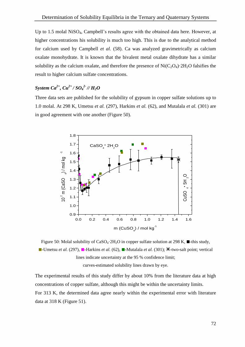
Determination of Solubility Equilibria in the Ternary and Quaternary Systems
72
Up to 1.5 molal NiSO4, Campbell’s results agree with the obtained data here. However, at
higher concentrations his solubility is much too high. This is due to the analytical method
for calcium used by Campbell et al. (58). Ca was analyzed gravimetrically as calcium
oxalate monohydrate. It is known that the bivalent metal oxalate dihydrate has a similar
solubility as the calcium oxalate, and therefore the presence of Ni(C2O4)·2H2O falsifies the
result to higher calcium sulfate concentrations.
System Ca2+
, Cu2+
/ SO42-
// H2O
Three data sets are published for the solubility of gypsum in copper sulfate solutions up to
1.0 molal. At 298 K, Umetsu et al. (297), Harkins et al. (62), and Mutalala et al. (301) are
in good agreement with one another (Figure 50).
0.0 0.2 0.4 0.6 0.8 1.0 1.2 1.4 1.6
0.9
1.0
1.1
1.2
1.3
1.4
1.5
1.6
1.7
1.8
CaSO4
2H2O
CuS
O4
5
H2O
102 m
(C
aSO
4)
/ mol
kg
-1
m (CuSO4) / mol kg
-1
Figure 50: Molal solubility of CaSO4·2H2O in copper sulfate solution at 298 K, -this study,
-Umetsu et al. (297), -Harkins et al. (62), -Mutalala et al. (301); -two-salt point; vertical
lines indicate uncertainty at the 95 % confidence limit;
curves-estimated solubility lines drawn by eye.
The experimental results of this study differ by about 10% from the literature data at high
concentrations of copper sulfate, although this might be within the uncertainty limits.
For 313 K, the determined data agree nearly within the experimental error with literature
data at 318 K (Figure 51).

Determination of Solubility Equilibria in the Ternary and Quaternary Systems
73
The data points given by Umetsu et al. are in terms of molarities, which were converted to
molalities in this study using the densities of copper sulfate solutions (266).
0.0 0.2 0.4 0.6 0.8 1.0 1.2 1.4 1.6 1.8 2.0
1.0
1.1
1.2
1.3
1.4
1.5
1.6
1.7
1.8
1.9
CuS
O4
5
H2O
CaSO4
2H2O
10
2 m
(C
aSO
4)
/ mol
kg
-1
m (CuSO4) / mol kg
-1
Figure 51: Molal solubility of CaSO4·2H2O in CuSO4 solutions at 313 K, -this study, -Umetsu
et al. (297) at 318 K, -Mutalala et al. (301) at 318 K; -two-salt point; vertical lines indicate
uncertainty at the 95 % confidence limit; curves-estimated solubility lines drawn by eye.
System Ca2+
, Zn2+
/ SO42-
// H2O
The system Ca2+
, Zn2+
/ SO42-
// H2O was examined by Umetsu et al. (297), Mutalala et al.
(81) and Hagemann (302) at 298 K. For higher temperatures, data were published by
Umetsu et al. (297) and by Mutalala et al. (81). The data of Hagemann range to high zinc
sulfate concentrations without reaching the saturation point of zinc sulfate (Figure 52).
There is considerable scatter in the data. The upper limit of Umetsu’s and Mutalala’s
measurements is 1.7 molal ZnSO4. Between these three data sets rough agreement exists.
The data of this study lie between Hagemann’s and Mutalala’s solubility curves. For zinc
sulfate solutions up to 0.5 molal, good agreement with Mutalala et al. is evident.
At 313 K, no direct comparison with literature data can be drawn. Umetsu et al. and
Mutalala et al. determined the gypsum solubility for 318 K.

Determination of Solubility Equilibria in the Ternary and Quaternary Systems
74
0.0 0.5 1.0 1.5 2.0 2.5 3.0 3.5 4.0
0.4
0.6
0.8
1.0
1.2
1.4
1.6
1.8
ZnSO4
7H2O
CaSO4
2H2O
102 m
(C
aSO
4)
/ mol
kg
-1
m (ZnSO4) / mol kg
-1
Figure 52: Molal gypsum solubility in zinc sulfate solution at 298 K; -this study, -Umetsu et al.
(297), -Hagemann (302), -Mutalala et al. (81); -two-salt point; vertical lines indicate
uncertainty at the 95 % confidence limit; curves-estimated solubility lines drawn by eye.
0.0 0.5 1.0 1.5 2.0 2.5 3.0 3.5 4.0 4.5
0.4
0.6
0.8
1.0
1.2
1.4
1.6
1.8
ZnSO4
6H2O
CaSO4
2H2O
102 m
(C
aSO
4)
/ mol
kg
-1
m (ZnSO4) / mol kg
-1
Figure 53: Molal gypsum solubility in zinc sulfate solution at 313 K; -this study, -Umetsu et al.
(297) at 318 K, -Mutalala et al. (81) at 318 K; -two-salt point; vertical lines indicate
uncertainty at the 95 % confidence limit; curves-estimated solubility lines drawn by eye.
Determination of Solubility Equilibria in the Ternary and Quaternary Systems
75
Figure 53 shows that the determined data resemble the values of Umetsu et al. (297) and
Mutalala et al. (81) within error except for the last data point given. Umetsu et al.
published his investigations in terms of mol/L solution. With the densities of Söhnel et al.
(266) the values were converted to molalities.
4.4. Quaternary Systems K+, Ca
2+, M
2+ / SO4
2- // H2O
(M = Mg, Mn, Co, Ni, Cu, Zn)
4.4.1. Experimental Procedures - K+, Ca
2+, M
2+ / SO4
2- // H2O
Studies of the quaternary systems were carried out at 313 K. Solutions with varying
concentrations were prepared by weighing different amounts of potassium sulfate and
bivalent metal sulfate into waterproof, firmly sealed bottles.
The general experimental procedure is described in section 4.1. After 48 h in the
thermostat, 0.5 g or 0.02 g of calcium sulfate hemihydrate was added. The samples were
kept stirring for another 24 h at 313 K. If no precipitation had been occurred over this time
a further 0.02 g of calcium sulfate hemihydrate was added. This procedure was repeated
until a solid phase formed. The amount of hemihydrate added was chosen in such a way
that the potassium sulfate concentration and the bivalent metal sulfate concentration were
changed by not more than the analytical error.
The samples remained in the thermostat for up to 90 days but at least for 46 days,
equilibrating after precipitation was detected.
4.4.2. Results - K+, Ca
2+, M
2+ / SO4
2- // H2O (M = Mg, Mn, Co, Ni, Cu, Zn)
The determined data are summarized in Appendix B – Experimental Results in Table 47 to
Table 52 and plotted in Figure 54. For calcium, an analytical error of up to 7 % of the
total concentration is indicated. The analytical error of potassium and nickel is within
1 to 1.5 % of the total molality. Results for the other metal ions (Mg, Mn, Co, Cu, Zn)
have an analytical error of 0.5 to 1% of the total concentration.

Determination of Solubility Equilibria in the Ternary and Quaternary Systems
76
In the examined concentration range, polyhalites K2SO4·MSO4·2CaSO4·2H2O crystallized
in all systems except for M = Ni. The absence of a polyhalite in the nickel system can be
attributed to the low solubility of K2SO4·NiSO4·6H2O. The fields of the polyhalites are
surrounded by the corresponding bivalent metal sulfate hydrate and the Tutton’s salt at
high bivalent metal sulfate concentrations. In the case of the system
K+, Ca
2+, Mn
2+ / SO4
2- // H2O, K2SO4·2MnSO4 appears instead of K2SO4·MnSO4·6H2O.
Leightonite, K2SO4·CuSO4·2CaSO4·2H2O, and Zn-polyhalite extend to small
concentrations of bivalent heavy metal sulfate and potassium sulfate. Investigations of the
magnesium-, manganese- and cobalt-containing systems showed that at small
concentrations of potassium sulfate the polyhalite field is restrained by gypsum. Limitation
of the polyhalite field at small concentrations of bivalent metal sulfate was not found
within the examined concentration range. At 313 K, gypsum appears only as a metastable
solid phase at high concentrations of bivalent metal sulfate.
The solubility curves of the metal sulfate hydrates and of the Tutton’s salt, as well as of
K2SO4·2MnSO4, with polyhalite do not vary noticeably from the solubility isotherm in the
ternary systems K+, M
2+ / SO4
2- // H2O at 313 K. The same is encountered for the solubility
curve of gypsum and polyhalite in comparison to the systems Ca2+
, M2+
/ SO42-
// H2O. The
heavy metal-containing systems equilibrate faster than do the solutions with magnesium.
This was noticed especially in solutions with low concentrations of bivalent metal sulfate.
The plots of calcium sulfate versus the concentration of MSO4 (M = Mg, Mn, Co, Ni, Cu,
Zn) show (Figure 55) that the crystallization field of leightonite extends to small
concentrations of CaSO4 (4·10-4
molal), whereas Mn-polyhalite extends only to
4·10-3
molal.
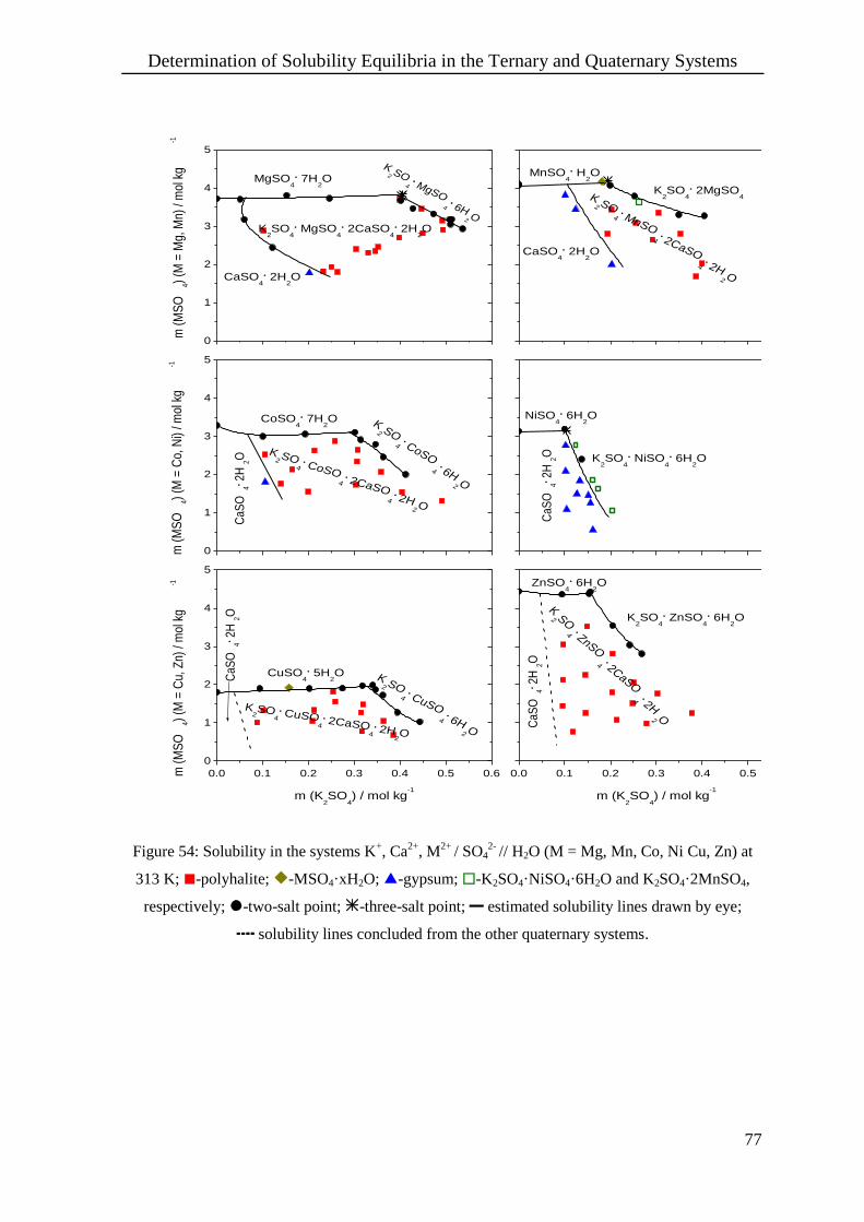
Determination of Solubility Equilibria in the Ternary and Quaternary Systems
77
0
1
2
3
4
5
0
1
2
3
4
5
0.0 0.1 0.2 0.3 0.4 0.5 0.6
0
1
2
3
4
5
0.0 0.1 0.2 0.3 0.4 0.5 0.6
K2SO
4
MgSO4
2CaSO4
2H2O
K2 SO
4 MgSO
4 6H
2 O
CaSO4
2H2O
MgSO4
7H2O
m (
MS
O4)
(M =
Mg,
Mn)
/ m
ol k
g-1
K2 SO
4 MnSO
4 2CaSO
4 2H
2 O
CaSO4
2H2O
K2SO
4
2MgSO4
MnSO4
H2O
CaS
O4 2
H2O K
2SO
4
NiSO4
6H2O
NiSO4
6H2O
K2SO
4 CoSO
4 2CaSO
4 2H
2O
CaS
O4
2H
2O
K2 SO
4 CoSO
4 6H
2 O
CoSO4
7H2O
m (
MS
O4)
(M =
Co,
Ni)
/ mol
kg
-1
CaS
O4
2H
2O
K2SO
4
CuSO4
2CaSO4
2H2O
K2 SO
4 CuSO
4 6H
2 O
CuSO4
5H2O
m (
MS
O4)
(M =
Cu,
Zn)
/ m
ol k
g-1
m (K2SO
4) / mol kg
-1
CaS
O4 2
H2O
K2 SO
4 ZnSO
4 2CaSO
4 2H
2 O
K2SO
4
ZnSO4
6H2O
ZnSO4
6H2O
m (K2SO
4) / mol kg
-1
Figure 54: Solubility in the systems K+, Ca
2+, M
2+ / SO4
2- // H2O (M = Mg, Mn, Co, Ni Cu, Zn) at
313 K; -polyhalite; -MSO4·xH2O; -gypsum; -K2SO4·NiSO4·6H2O and K2SO4·2MnSO4,
respectively; -two-salt point; -three-salt point; estimated solubility lines drawn by eye;
solubility lines concluded from the other quaternary systems.
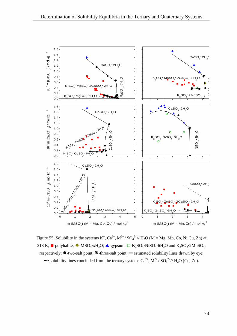
Determination of Solubility Equilibria in the Ternary and Quaternary Systems
78
0.0
0.2
0.4
0.6
0.8
1.0
1.2
1.4
1.6
1.8
0.0
0.2
0.4
0.6
0.8
1.0
1.2
1.4
1.6
1.8
0 1 2 3 4 5
0.0
0.2
0.4
0.6
0.8
1.0
1.2
1.4
1.6
1.8
0 1 2 3 4 5
K2SO
4
MgSO4
2CaSO4
2H2O
CaSO4
2H2O
MgS
O4 7
H2O
K2SO
4
MgSO4
6H2O
K2SO
4
MnSO4
2CaSO4
2H2O
CaSO4
2H2O
MnS
O4 H
2O
K2SO
4
2MnSO4
K2SO
4
CoSO4
6H2O
CoS
O4
7H
2O
K 2SO 4
CoSO 4
2CaSO 4
2H 2O
CaSO4
2H2O
102 m
(C
aSO
4)
/ mol
kg
-1
102 m
(C
aSO
4)
/ mol
kg
-1
K2SO
4
CuSO4
6H2O
CuS
O4
5H
2O
K 2SO
4 C
uSO
4 2
CaS
O4
2H
2O
CaSO4
2H2O
102 m
(C
aSO
4)
/ mol
kg
-1
m (MSO4) (M = Mg, Co, Cu) / mol kg
-1
K2SO
4
ZnSO4
6H2O Z
nSO
4 6
H2O
K2SO
4
ZnSO4
2CaSO4
2H2O
CaSO4
2H2O
m (MSO4) (M = Mn, Zn) / mol kg
-1
CaSO4
2H2O
K2SO
4
NiSO4
6H2O
NiS
O4
6H
2O
Figure 55: Solubility in the systems K+, Ca
2+, M
2+ / SO4
2- // H2O (M = Mg, Mn, Co, Ni Cu, Zn) at
313 K; -polyhalite; -MSO4·xH2O; -gypsum; -K2SO4·NiSO4·6H2O and K2SO4·2MnSO4,
respectively; -two-salt point; -three-salt point; estimated solubility lines drawn by eye;
solubility lines concluded from the ternary systems Ca2+
, M2+
/ SO42-
// H2O (Cu, Zn).
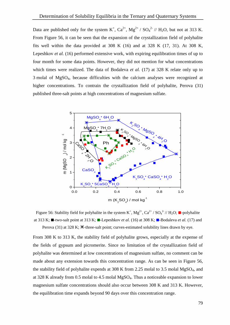
Determination of Solubility Equilibria in the Ternary and Quaternary Systems
79
Data are published only for the system K+, Ca
2+, Mg
2+ / SO4
2- // H2O, but not at 313 K.
From Figure 56, it can be seen that the expansion of the crystallization field of polyhalite
fits well within the data provided at 308 K (16) and at 328 K (17, 31). At 308 K,
Lepeshkov et al. (16) performed extensive work, with expiring equilibration times of up to
four month for some data points. However, they did not mention for what concentrations
which times were realized. The data of Bodaleva et al. (17) at 328 K relate only up to
3 molal of MgSO4, because difficulties with the calcium analyses were recognized at
higher concentrations. To contrain the crystallization field of polyhalite, Perova (31)
published three-salt points at high concentrations of magnesium sulfate.
0.0 0.2 0.4 0.6 0.8 1.0
0
1
2
3
4
5
K 2SO 4
CaSO 4
H 2O
K2SO
4
CaSO4
H2O
K2SO
4
5CaSO4
H2O
CaSO4
CaSO
4
2H2 O
MgSO4
7H2O
MgSO4
6H2O
K2 SO
4
MgSO4
4H2 O
K2 SO
4
MgSO4
6H2 O
Ph
m (
MgS
O4)
/ mol
kg
-1
m (K2SO
4) / mol kg
-1
Figure 56: Stability field for polyhalite in the system K+, Mg
2+, Ca
2+ / SO4
2- // H2O; -polyhalite
at 313 K; -two-salt point at 313 K; -Lepeshkov et al. (16) at 308 K; -Bodaleva et al. (17) and
Perova (31) at 328 K; -three-salt point; curves-estimated solubility lines drawn by eye.
From 308 K to 313 K, the stability field of polyhalite grows, especially at the expense of
the fields of gypsum and picromerite. Since no limitation of the crystallization field of
polyhalite was determined at low concentrations of magnesium sulfate, no comment can be
made about any extension towards this concentration range. As can be seen in Figure 56,
the stability field of polyhalite expends at 308 K from 2.25 molal to 3.5 molal MgSO4, and
at 328 K already from 0.5 molal to 4.5 molal MgSO4. Thus a noticeable expansion to lower
magnesium sulfate concentrations should also occur between 308 K and 313 K. However,
the equilibration time expands beyond 90 days over this concentration range.
Determination of Solubility Equilibria in the Ternary and Quaternary Systems
80
4.5. Decomposition of Polyhalite in Solutions of the System
K+, Ca
2+, Mg
2+ / SO4
2- // H2O
4.5.1. Experimental Procedures - Decomposition of Polyhalite
The dissolution of polyhalite in solutions containing varying concentrations of the ions
K+, Ca
2+, Mg
2+, and SO4
2- was followed at 303 K. For this, different amounts of
MgSO4·7H2O were weighed into glass bottles with a volume of 2 mL. Different
concentrations of potassium sulfate and calcium sulfate were prepared from stock solutions
of m = 0.45 molal K2SO4 and m = 0.013 molal CaSO4, respectively. For higher
concentrations of K2SO4, solid salt was added. Finally, deionized water (Seralpur
Pro 90 CN) was added to obtain the appropriate concentrations of the ions in solution,
taking into account the water added before with MgSO4·7H2O and the stock solutions of
potassium sulfate and calcium sulfate. The stock solutions were prepared from appropriate
masses of deionized water and gypsum or potassium sulfate.
The waterproof, tightly sealed glass bottles were placed in a sample holder with an array of
50 samples. The sample holder was sealed and then lowered into a thermostatted water
bath until it was covered. The bottles were aligned horizontally to facilitate mixing by
shaking. The solutions were kept in the water bath for at least 48 h at 303 K, before adding
around 0.02 g of polyhalite to the solution. The polyhalites were prepared as described in
section 9.1. The dissolution experiments lasted up to 82 days. During this time the
solutions were shaken thoroughly. The water bath had a temperature uncertainty of
± 0.1 K.
To separate the solid from the solution, the sample holder with the glass bottles was placed
on a platform positioned in the thermostat. This way the samples could be opened and still
kept at reaction temperature. A frit with a glass fiber membrane (0.6 µm, MN 85/70,
Macherey & Nagel) was lowered into a bottle and the solid separated by suction filtration.
The solid on the frit was washed with 85 % and 96 % ethanol, and then air dried.
Afterward, the solid was analyzed by Raman spectroscopy using the frit as sample holder.
The concentration of the separated solution was not determined.
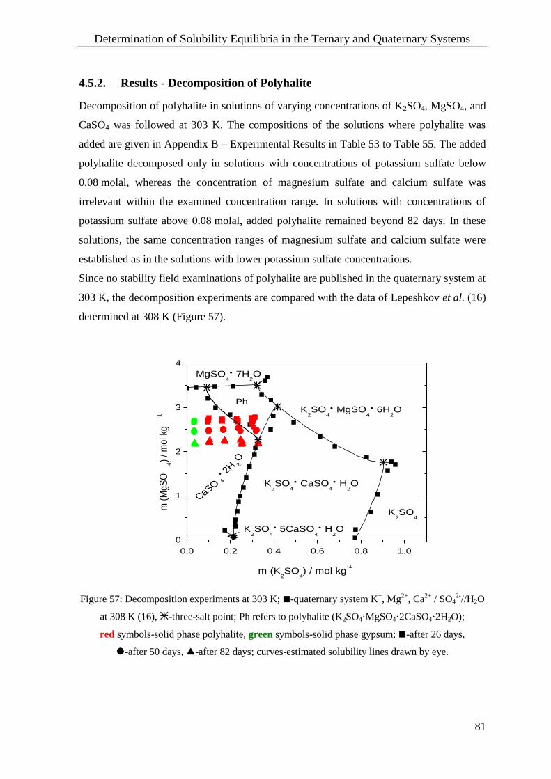
Determination of Solubility Equilibria in the Ternary and Quaternary Systems
81
4.5.2. Results - Decomposition of Polyhalite
Decomposition of polyhalite in solutions of varying concentrations of K2SO4, MgSO4, and
CaSO4 was followed at 303 K. The compositions of the solutions where polyhalite was
added are given in Appendix B – Experimental Results in Table 53 to Table 55. The added
polyhalite decomposed only in solutions with concentrations of potassium sulfate below
0.08 molal, whereas the concentration of magnesium sulfate and calcium sulfate was
irrelevant within the examined concentration range. In solutions with concentrations of
potassium sulfate above 0.08 molal, added polyhalite remained beyond 82 days. In these
solutions, the same concentration ranges of magnesium sulfate and calcium sulfate were
established as in the solutions with lower potassium sulfate concentrations.
Since no stability field examinations of polyhalite are published in the quaternary system at
303 K, the decomposition experiments are compared with the data of Lepeshkov et al. (16)
determined at 308 K (Figure 57).
0.0 0.2 0.4 0.6 0.8 1.0
0
1
2
3
4
K2SO
4
5CaSO4
H2O
PhK
2SO
4
MgSO4
6H2O
K2SO
4
CaSO4
H2O
K2SO
4
MgSO4
7H2O
CaSO4
2H 2
O
m (
MgS
O4)
/ mol
kg
-1
m (K2SO
4) / mol kg
-1
Figure 57: Decomposition experiments at 303 K; -quaternary system K+, Mg
2+, Ca
2+ / SO4
2-//H2O
at 308 K (16), -three-salt point; Ph refers to polyhalite (K2SO4·MgSO4·2CaSO4·2H2O);
red symbols-solid phase polyhalite, green symbols-solid phase gypsum; -after 26 days,
-after 50 days, -after 82 days; curves-estimated solubility lines drawn by eye.

Determination of Solubility Equilibria in the Ternary and Quaternary Systems
82
The stability field of polyhalite at 303 K is seen to be smaller then at 308 K. Therefore,
polyhalite should not be stable in most of the solutions and should decompose. The
experiments showed that polyhalite decomposed into gypsum only at very small potassium
sulfate concentrations. Even after 82 days polyhalite remained in solutions with higher
concentrations of K2SO4. This would confirm the statement of D’Ans (307), that polyhalite
forms and decomposes slowly. Lepeshkov et al. (16) wrote that polyhalite decomposed fast
in non-stable solutions under the conditions they employed. However, they did not give
any information about the origin of their polyhalite. Some years before, the same research
group examined the stability field of polyhalite at 328 K, using a polyhalite synthesized
according to the method of Basch (303). If they did not thoroughly wash this polyhalite,
traces of chloride would remain, and which could hasten the decomposition of polyhalite.
Determination of the Enthalpies of Dissolution
83
5. Determination of the Enthalpies of Dissolution of the
Polyhalites at Infinite Dilution
5.1. Experimental Procedures - Enthalpies of Dissolution
The triple salts K2SO4·MSO4·2CaSO4·2H2O (M = Mg, Mn, Co, Ni, Cu, Zn) were prepared
as described in section 9.1. Copper sulfate pentahydrate and potassium sulfate, used in the
calorimetric measurements, were re-crystallized and examined using powder X-ray
diffraction, and CuSO4·5H2O additionally by thermal analyses. The preparation of the
manganese sulfate monohydrate is described in section 9.1. NaClO4 and NaNO3 solutions
were prepared by weighing. The exact molality of the solutions used was calculated from
the masses of the salt and deionized water used for preparation. Sodium perchlorate
solutions were analyzed additionally by AAS.
Calorimetric experiments were performed using a Thermal Activity Monitor, TAM II,
Thermometric, Sweden, equipped with the precision solution 2225 calorimeter. The
enthalpy values were evaluated using the program Sol-Cal of the TAM software package.
In glass ampoules (V = 1 mL), the salt was weighed with a microbalance (CC20, 20 g/1 µg,
Sartorius), and afterward sealed with a silicone stopper and beeswax. The reaction vessel
was filled with 100 mL of the appropriate NaClO4 solution or NaNO3 solution, and
weighed with an electronic balance (ST 200, 200 g/0.1 mg, Ströhlein). The amounts of the
polyhalites, potassium sulfate and NaClO4 solution were chosen well below the saturation
concentration of KClO4.
All measurements were carried out at 298.15 K. The reaction vessel containing the
ampoule was thermostatted in the calorimeter under constant stirring speed (500 rpm).
With an electric heater in the reaction vessel, thermal equilibration between the reaction
vessel and the thermostat bath was accelerated. After reaching thermal equilibrium, the
reaction was started by breaking the ampoule. Since polyhalite and its analogues dissolve
slowly main- and after-periods ran for at least 4 h. For K2SO4, CuSO4·5H2O and
MnSO4·H2O, the duration of the periods was lowered to 90 min. At each NaClO4
concentration at least two measurements were performed. The thermostat stability was
0.1 mK over 24 h and the reaction vessel temperature stability was 0.05 mK over 10 h.
Calibration was performed directly after every dissolution experiment by means of electric
heating. The heating power was 100 mW and heating time 50 s.

Determination of the Enthalpies of Dissolution
84
Before the experiments were carried out, the breaking heat of the ampoule was found to be
0.4 % of the total heat effect in the dissolution experiments and was not explicitly
considered. The overall accuracy of the calorimeter was verified by measuring the enthalpy
of dissolution of ultra pure KCl, which was prepared and characterized as described by
Günther et al. (311). The measured molar enthalpy of dissolution was 17.46 kJ mol-1
. The
International Union of Pure and Applied Chemistry (IUPAC) published a recommended
reference enthalpy of dissolution of KCl as 17.584 0.017 kJ mol-1
(312).
5.2. Results - Enthalpies of Dissolution
Calorimetric data obtained are listed in Appendix B – Experimental Results in Table 56 to
Table 61 and plotted in Figure 58 to Figure 60.
0.0 0.5 1.0 1.5 2.0 2.5
-45
-40
-35
-30
-25
-20
-15
-10
so
lH /
kJ m
ol-1
m (NaClO4) / mol kg
-1
Figure 58: Integral molar heats of dissolution of the polyhalites in NaClO4 solution at 298 K;
-Mg-polyhalite, -Mn-polyhalite, -Co-polyhalite, -Ni-polyhalite,
-leightonite, -Zn-polyhalite.
All polyhalites dissolve exothermally. With increasing NaClO4 concentration, the integral
molar heat of dissolution becomes more exothermic for all polyhalites, by about
-15 kJ mol-1
within the concentration range from 0.5 molal NaClO4 to 2.2 molal NaClO4.
The slope of the regression lines in the SIT plot (Figure 61) is more or less the same for all
polyhalites.

Determination of the Enthalpies of Dissolution
85
In order to detrmine whether the strong concentration dependence could be caused by
hydrolytic or ion association effects of the bivalent metal sulfates, additional calorimetric
experiments were conducted with MnSO4·H2O and CuSO4·5H2O. From all ions considered
in this study, hydrated cupric ions possess the largest acidity constant (315). Ion
association constants are given in the literature (316, 317).
0.0 0.5 1.0 1.5 2.0 2.5
-40
-38
-36
-34
6
8
10
so
lH /
kJ m
ol-1
m (NaClO4) / mol kg
-1
Figure 59: Integral molar heats of dissolution of the MnSO4·H2O and CuSO4·5H2O, respectively, in
NaClO4 solution at 298 K; -MnSO4·H2O, -CuSO4·5H2O.
As can be seen in Figure 59, the dissolution enthalpies of CuSO4·5H2O and MnSO4·H2O
hardly vary within the concentration range. Therefore, the conclusion can be drawn that the
increasing exothermicity is not caused by the bivalent metal sulfates. Determinations of the
integral dissolution enthalpies of potassium sulfate in sodium perchlorate solutions,
ranging from 0.097 molal to 0.52 molal, showed the same strong concentration-
dependence on NaClO4 concentration as the polyhalites (Figure 60). To ensure that no
precipitation of potassium perchlorate occurs, which might cause this result, the integral
dissolution enthalpies of potassium sulfate were determined also in sodium nitrate
solutions of 0.47 molal and 3.3 molal. Again, within the concentration range considered,
the dissolution enthalpies become more exothermic by about -14 kJ mol-1
. Thus, the slope
of the dissolution enthalpies of the polyhalites is related with K2SO4 as a constituent of
polyhalite. However, the type of ion interaction responsible for the strong concentration
dependence is not entirely clear. Ion association for monovalent cations with sulfate anions

Determination of the Enthalpies of Dissolution
86
is discussed in the literature (318-321), but the enthalpy effects should be much smaller
than those in this study.
0.0 0.5 1.0 1.5 2.0 2.5 3.0 3.5
6
8
10
12
14
16
18
20
22
24
so
lH /
kJ m
ol-1
m (NaClO4, NaNO
3) / mol kg
-1
Figure 60: Integral molar heats of dissolution of the K2SO4 in NaClO4 and NaNO3 solution
at 298 K; -NaClO4, -NaNO3.
Systematic trends within the series of the polyhalites K2MCa2(SO4)4·2H2O (M = Mn, Co,
Ni, Cu, Zn) can hardly be discerned. The smallest enthalpy of dissolution is observed for
leightonite. Co-polyhalite can, however, be distinguished clearly from all other salts
(Figure 58).
Extrapolation of the integral molal heats of dissolution solHm to infinite dilution was
performed using the SIT model (13).
The concentration dependence of the enthalpy of dissolution solHm can be described with
i
imimmsolmsol LLHH ,2,1,1 [50]
where 1 denotes the solvent, 2 the solute and i the stoichiometric coefficient. The relative
partial molar enthalpy of the solvent L1 in NaClO4 solutions can be expressed with Pitzer’s
equation (12)
L
NaClONaNa
IL
NaClO
L
NaClOClONa
m
mL
OH
m
mCzemRT
I
IAM
L
m
4444
2
22
)2.11(21000
1022
23
1,
[42]
Determination of the Enthalpies of Dissolution
87
where m is the molality of NaClO4. Pitzer’s enthalpy parameters for NaClO4 are
L (0) = 1.296·10
-5, L (1)
= 2.29·10-5
, CL = -8.1·10
-5 (12) with = 2. The Debye-Hückel
slope of AL of 298 K was calculated with the polynomial given by Beyer (313), which is
based on the equation of Archer et al. (14).
For the calculation of the relative partial molal enthalpy of the solute, the SIT model was
used (13).
)(
5.114
3 2
2
,2, ijmRT
I
IzAL Li
m
miL
iim
[47]
From equation [50] and [47] the following is derived.
i
Li
i
ii
m
mL
mmsolmsol ijmRTz
I
IALHH )(
5.114
3 22
1,1 [51]
Linearization then gives
)(2
1,1 ijmRTHDLH Lmsolmmsol [52]
with
i
ii
m
mLz
I
IAD 2
5.114
3 [53]
and
i
LiL ij)( [54]
Figure 61 shows the linear, unweighted regression lines for the results and their
extrapolation to infinite dilution. The resulting standard enthalpies of solution are
summarized in Table 16.
Within the limits of experimental uncertainty, the enthalpies coincide for the polyhalites
with M = Mg, Mn, Ni, Zn. The value for the cobalt salt is noticeable less exothermic.
Leightonite, which does not crystallize with the polyhalite structure (322), possesses a
considerably different dissolution enthalpy.
Richardson et al. (310) published the heat effect of decomposing 5 g of polyhalite in 5 g of
water. Since polyhalite is an incongruently soluble salt, decomposing in water into gypsum
plus solution, the data cannot be used for comparison.
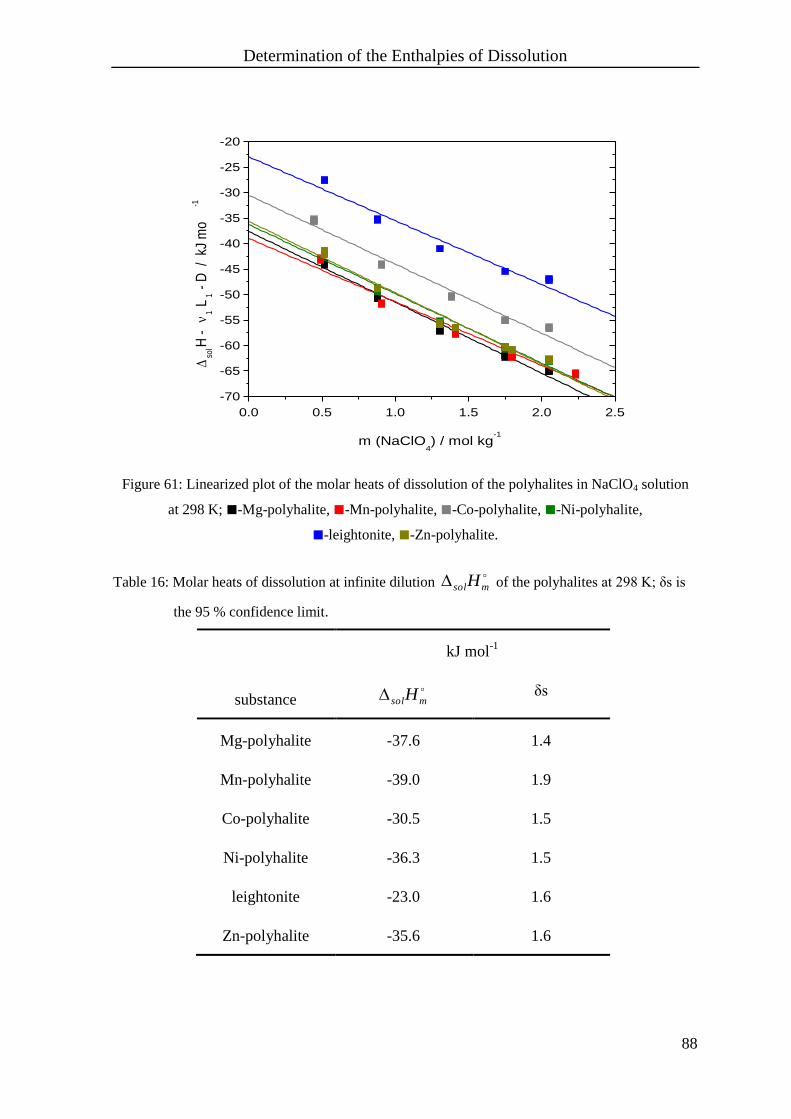
Determination of the Enthalpies of Dissolution
88
0.0 0.5 1.0 1.5 2.0 2.5
-70
-65
-60
-55
-50
-45
-40
-35
-30
-25
-20
so
lH -
1 L
1 -
D /
kJ
mo
-1
m (NaClO4) / mol kg
-1
Figure 61: Linearized plot of the molar heats of dissolution of the polyhalites in NaClO4 solution
at 298 K; -Mg-polyhalite, -Mn-polyhalite, -Co-polyhalite, -Ni-polyhalite,
-leightonite, -Zn-polyhalite.
Table 16: Molar heats of dissolution at infinite dilution msolH of the polyhalites at 298 K; δs is
the 95 % confidence limit.
kJ mol-1
substance msolH δs
Mg-polyhalite -37.6 1.4
Mn-polyhalite -39.0 1.9
Co-polyhalite -30.5 1.5
Ni-polyhalite -36.3 1.5
leightonite -23.0 1.6
Zn-polyhalite -35.6 1.6

Estimation of Pitzer Parameters
89
6. Estimation of Pitzer Parameters
6.1. Parameters for Pure Electrolytes
6.1.1. Binary Parameters of MSO4 (M = Mn, Co, Ni, Cu, Zn) at 298 K
In Chapter 3, literature review, the published parameters for the pure electrolytes MSO4
(M = Mn, Co, Ni, Cu, Zn) were examined. Evaluation of the different parameter sets is
based on the deviation = cal - exp calculated from experimental osmotic coefficients
and from values obtained with Pitzer’s equation with the various parameter sets. The
parameters with the smallest deviation from the experimental data are summarized in
Table 17 and used in this study.
In the case of cobalt sulfate, a considerable difference occurred between the experimentally
determined osmotic coefficients and the ones calculated with Pitzer’s equation and the
parameter set of Filippov et al. (243). Thus, a new evaluation was necessary.
Table 17: Pitzer parameters for M2+
-SO42-
(M = Mn, Ni, Cu, Zn) at 298 K; 1 = 1.4, 2 = 12.
M 0
MX 1
MX 2
MX MXC
Ref.
Mn 0.2065 2.9511 -40 0.01636 (114)
Ni 0.1625 2.903 -51.54 0.0389 (233)
Cu 0.21757 2.62597 -56.2413 0.013756 (247)
Zn 0.1849 2.9614 -55.8433 0.0324 (250)
Binary Parameters of CoSO4 at 298 K
There are two different data sets of osmotic coefficients (236, 164) measured in the
concentration range between 0.1 molal and 2.4693 molal CoSO4. The data of Balarev et al.
(164) decrease noticeably at concentrations below 1.0 molal CoSO4 (Figure 62). Above
this concentration the osmotic coefficient rises almost linearly, unlike the values of Libus
et al. (236). Activity coefficients were determined up to 1.0 molal CoSO4 (323-325). The
values given by Haring et al. (325) differ increasingly with rising concentration and higher
activity coefficients (Figure 63).
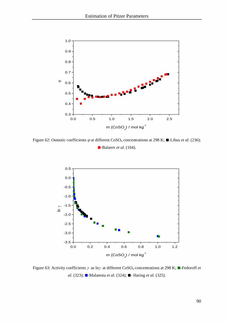
Estimation of Pitzer Parameters
90
0.0 0.5 1.0 1.5 2.0 2.5
0.3
0.4
0.5
0.6
0.7
0.8
0.9
1.0
m (CoSO4) / mol kg
-1
Figure 62: Osmotic coefficients at different CoSO4 concentrations at 298 K; -Libus et al. (236);
-Balarev et al. (164).
0.0 0.2 0.4 0.6 0.8 1.0 1.2
-3.5
-3.0
-2.5
-2.0
-1.5
-1.0
-0.5
0.0
0.5
ln
m (CoSO4) / mol kg
-1
Figure 63: Activity coefficients as ln at different CoSO4 concentrations at 298 K; -Fedoroff et
al. (323); -Malatesta et al. (324); - Haring et al. (325).
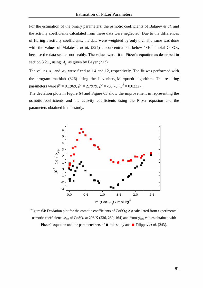
Estimation of Pitzer Parameters
91
For the estimation of the binary parameters, the osmotic coefficients of Balarev et al. and
the activity coefficients calculated from these data were neglected. Due to the differences
of Haring’s activity coefficients, the data were weighted by only 0.2. The same was done
with the values of Malatesta et al. (324) at concentrations below 1·10-1
molal CoSO4,
because the data scatter noticeably. The values were fit to Pitzer’s equation as described in
section 3.2.1, using A as given by Beyer (313).
The values 1 and 2 were fixed at 1.4 and 12, respectively. The fit was performed with
the program mathlab (326) using the Levenberg-Marquardt algorithm. The resulting
parameters were β0 = 0.1969, β
1 = 2.7979, β
2 = -58.70, C
= 0.02327.
The deviation plots in Figure 64 and Figure 65 show the improvement in representing the
osmotic coefficients and the activity coefficients using the Pitzer equation and the
parameters obtained in this study.
0.0 0.5 1.0 1.5 2.0 2.5
-3
-2
-1
0
1
2
3
4
5
6
102
/
exp
m (CoSO4) / mol kg
-1
Figure 64: Deviation plot for the osmotic coefficients of CoSO4; calculated from experimental
osmotic coefficients exp of CoSO4 at 298 K (236, 239, 164) and from calc values obtained with
Pitzer’s equation and the parameter sets of -this study and -Filippov et al. (243).
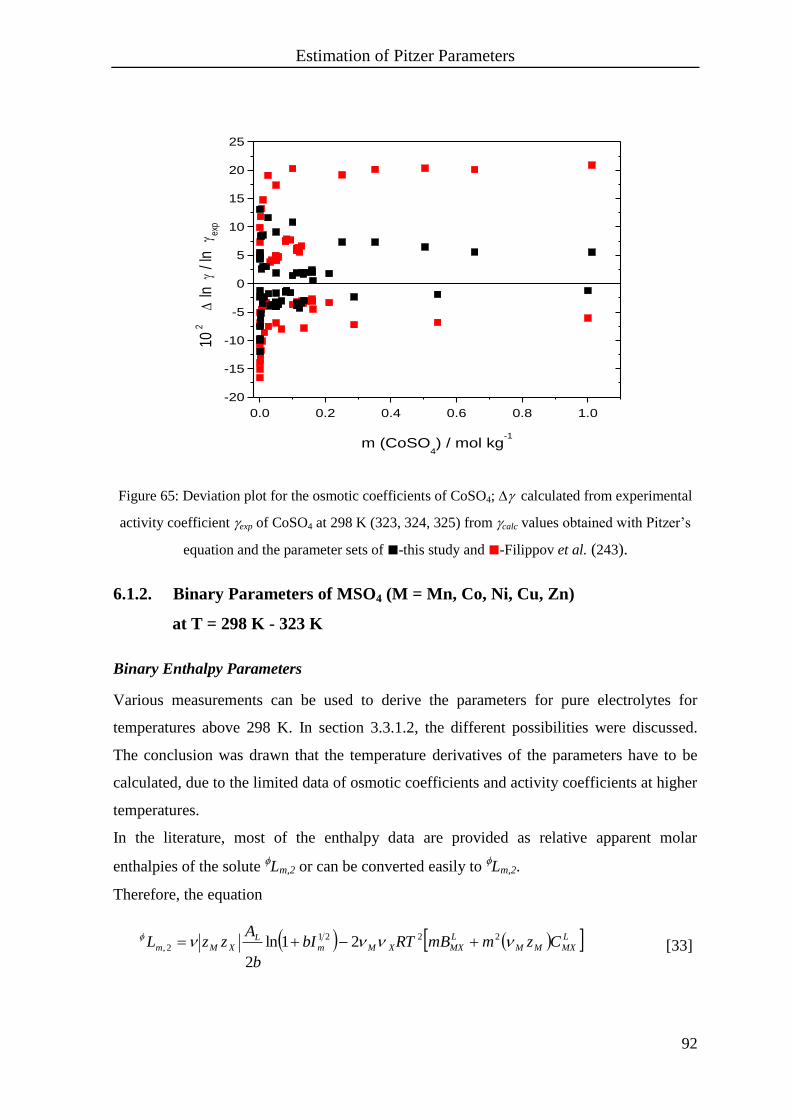
Estimation of Pitzer Parameters
92
0.0 0.2 0.4 0.6 0.8 1.0
-20
-15
-10
-5
0
5
10
15
20
25
102
ln
/ ln
ex
p
m (CoSO4) / mol kg
-1
Figure 65: Deviation plot for the osmotic coefficients of CoSO4; calculated from experimental
activity coefficient exp of CoSO4 at 298 K (323, 324, 325) from calc values obtained with Pitzer’s
equation and the parameter sets of -this study and -Filippov et al. (243).
6.1.2. Binary Parameters of MSO4 (M = Mn, Co, Ni, Cu, Zn)
at T = 298 K - 323 K
Binary Enthalpy Parameters
Various measurements can be used to derive the parameters for pure electrolytes for
temperatures above 298 K. In section 3.3.1.2, the different possibilities were discussed.
The conclusion was drawn that the temperature derivatives of the parameters have to be
calculated, due to the limited data of osmotic coefficients and activity coefficients at higher
temperatures.
In the literature, most of the enthalpy data are provided as relative apparent molar
enthalpies of the solute Lm,2 or can be converted easily to
Lm,2.
Therefore, the equation
L
MXMM
L
MXXMmL
XMm CzmmBRTbI
b
AzzL 2221
2, 21ln
2
[33]
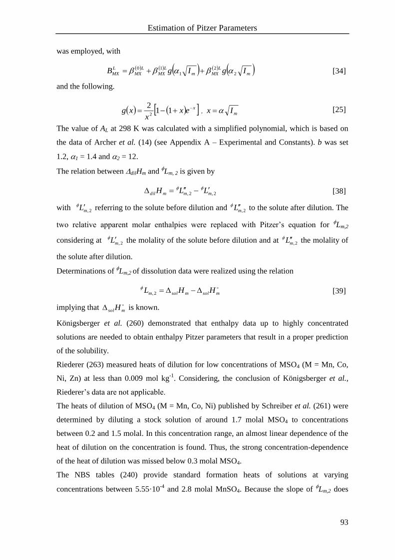
Estimation of Pitzer Parameters
93
was employed, with
m
L
MXm
L
MX
L
MX
L
MX IgIgB 2
2
1
10 [34]
and the following.
xexx
xg 112
2, mIx [25]
The value of AL at 298 K was calculated with a simplified polynomial, which is based on
the data of Archer et al. (14) (see Appendix A – Experimental and Constants). b was set
1.2, 1 = 1.4 and 2 = 12.
The relation between dilHm and Lm, 2 is given by
2,2, mmmdil LLH [38]
with 2,mL referring to the solute before dilution and 2,mL to the solute after dilution. The
two relative apparent molar enthalpies were replaced with Pitzer’s equation for Lm,2
considering at 2,mL the molality of the solute before dilution and at 2,mL the molality of
the solute after dilution.
Determinations of Lm,2 of dissolution data were realized using the relation
msolmsolm HHL 2,
[39]
implying that msolH is known.
Königsberger et al. (260) demonstrated that enthalpy data up to highly concentrated
solutions are needed to obtain enthalpy Pitzer parameters that result in a proper prediction
of the solubility.
Riederer (263) measured heats of dilution for low concentrations of MSO4 (M = Mn, Co,
Ni, Zn) at less than 0.009 mol kg-1
. Considering, the conclusion of Königsberger et al.,
Riederer’s data are not applicable.
The heats of dilution of MSO4 (M = Mn, Co, Ni) published by Schreiber et al. (261) were
determined by diluting a stock solution of around 1.7 molal MSO4 to concentrations
between 0.2 and 1.5 molal. In this concentration range, an almost linear dependence of the
heat of dilution on the concentration is found. Thus, the strong concentration-dependence
of the heat of dilution was missed below 0.3 molal MSO4.
The NBS tables (240) provide standard formation heats of solutions at varying
concentrations between 5.55·10-4
and 2.8 molal MnSO4. Because the slope of Lm,2 does
Estimation of Pitzer Parameters
94
not change considerably at concentrations above 1.0 molal MnSO4, the data range of
MnSO4 is sufficient.
In the literature, only a few data points of CoSO4 are available. Schreiber et al. (261)
published integral molar heats of dilution as described before. In the NBS tables (240) only
four data points are given. Thus it is not possible to determine enthalpy parameters for
CoSO4. Comparison of the relative apparent molar enthalpy of CoSO4 solutions with data
for nickel sulfate solutions revealed similar behavior (Figure 69).
Heat of dilution data for NiSO4 are published by Schreiber et al. (261) and Soloveva et al.
(264), who calculated also relative apparent molar enthalpies from the measured heats of
dilution. For a small concentration range Goldberg et al. (265) determined heats of
dissolution of nickel sulfate hexahydrate. With the standard heat of dissolution given by
Goldberg et al. for NiSO4·6H2O relative apparent molar enthalpies were calculated. The
data vary considerably from values provided by the NBS tables (240) and have been
neglected, for that reason.
Two data sets for relative apparent molar enthalpies of copper sulfate solutions can be
derived from the literature at 298 K. Lange et al. (267) measured heats of dilution and
calculated from these values relative apparent molar enthalpies. The other data set is given
in the NBS tables (240) as standard formation enthalpies of solutions at different
concentrations. The data point of the NBS tables for 1.11 molal CuSO4 differs from the
data of Lange et al. (267) and was neglected therefore.
The system Zn2+
/ SO42-
// H2O is the best investigated one regarding the enthalpy. Relative
apparent molar enthalpies at concentrations between 0.0001 and 1 molal ZnSO4 were
provided by Lange et al. (267) calculated from integral heats of dilution. At concentrations
above 1 molal Giauque et al. (268) published relative partial molar enthalpies of the solute
and the solvent. The data were recalculated to relative apparent molar enthalpies. As
mentioned in section 3.3.1.2, Harned (269) re-estimated the data given by Cowperthwaite
et al. (258). Since the relative partial molar enthalpies of the solvent are not published by
Harned the relative apparent molar enthalpies cannot be calculated. In the NBS tables, data
for the whole concentration range are given. However, the value in the NBS tables at
2.775 molal ZnSO4 deviates from the other data. Hence, this data point was neglected.
The data were fitted with the program mathlab (326) applying the Levenberg-Marquardt
algorithm. The fit of the enthalpy data is plotted in Figure 66 and Figure 67. Resulting
binary enthalpy parameters are given in Table 18.

Estimation of Pitzer Parameters
95
0.0 0.5 1.0 1.5 2.0 2.5 3.0 3.5 4.0 4.5
0
2
4
6
8
10
12
14
16
Mn
Ni
Cu
Zn
L
m, 2
/ kJ
mol
-1
m (MSO4) (M = Mn, Ni, Cu, Zn) / mol kg
-1
Figure 66: Relative apparent molar enthalpies for MSO4 (M = Mn, Ni, Cu, Zn) solutions;
-NBS tables (240); -Soloveva et al. (264); -Lange et al. (267); -Giauque et al. (268);
values obtained with Pitzer’s equation and the determined enthalpy parameters calculated up to
saturation of MSO4.
0 1 2 3 4 5
-10
-8
-6
-4
-2
0
2
4
6
8
Mn
Ni
di
lH (
kJ/m
ol)
m (MSO4) (M = Mn, Ni) / mol kg
-1
Figure 67: Integral molar heats of dilution for MSO4 (M = Mn, Ni) solutions, -Schreiber
et al. (261); values obtained with Pitzer’s equation and the determined enthalpy parameters
calculated up to saturation of MSO4.

Estimation of Pitzer Parameters
96
Table 18: Enthalpy Pitzer parameters for M2+
-SO42-
at 298 K.
M 103 0L
MX 10
2 1L
MX 101 2L
MX 104 L
MXC
Mn 1.070 0.7619 -5.793 -1.745
Ni 0.3289 1.546 -3.6869 -0.2488
Cu -1.270 1.675 -5.027 3.327
Zn 1.034 1.123 -3.094 -1.464
Königsberger et al. (260) determined his enthalpy parameters for zinc sulfate
( 0L
MX = 6.7·10-4
, 1L
MX = 1.297·10-2
, 2L
MX = -3.15·10-1
, L
MXC = -1.848·10-3
) only with data
provided in the NBS tables. From Figure 68, it can be seen that the new fit is better, since
the data of Lange et al. (267) and Giauque et al. (268) were taken also into account.
0.0 0.5 1.0 1.5 2.0 2.5 3.0 3.5 4.0
0
1
2
3
4
5
6
7
8
9
10
L
m, 2
/ kJ
mol
-1
m (ZnSO4) / mol kg
-1
Figure 68: Relative apparent molar enthalpies for ZnSO4 solutions at 298 K, -NBS tables (240);
-Lange et al. (267); -Giauque et al. (268); values obtained with Pitzer’s equation and the
enthalpy parameters of Königsberger et al. (260) and this study.

Estimation of Pitzer Parameters
97
Binary Parameters and Solubility Constants of the Solids for T = 283 K – 323 K
The enthalpy parameters are defined by temperature variation of the binary parameters of a
pure electrolyte by equations [35] and [36] (see section 3.2.1.1).
2,1,0,
i
Tp
i
MXiL
MX
[35]
p
MXL
MX T
CC
[36]
To derive binary parameters, the equations were integrated, resulting in equations [55]
and [56].
2,1,0,0, 0 iTTdT iL
MX
i
TMX
iL
MX
i
MX [55]
0, 0TTCCdTCC L
MXTMX
L
MXMX [56]
Applying equation [27] for 2-2 electrolytes MXMX CC 4 gives equation [57].
0, 440
TTCCdTCC L
MXTMX
L
MXMX [57]
T0 refers to 298 K. Thus, the binary Pitzer parameters of 298 K, i
TMX 0, and
0,TMXC
(Table 19), were employed, and parameters calculated in the temperature range from
283 K to 323 K. These parameters were fit to the linear equation
P = B + DT [58]
where P refers to any parameter of 0
MX , 1
MX , 2
MX and MXC . B and D denote the
temperature coefficients, which are summarized in Appendix C – Temperature-Dependent
Parameters in Table 62 to Table 71.
In the case of CoSO4, only limited enthalpy data have been published. A comparison of the
values of CoSO4 showed similarity with the values of NiSO4 (Figure 69 and Figure 70).
Therefore, the enthalpy parameters of NiSO4 were applied to derive the temperature-
dependent parameters of CoSO4.

Estimation of Pitzer Parameters
98
Table 19: Pitzer parameters for M2+
-SO42-
(M = Mn, Co, Ni, Cu, Zn) at 298 K; 1 = 1.4, 2 = 12.
Metal 0
MX 1
MX 2
MX MXC
Ref.
Mn 0.2065 2.9511 -40 0.01636 (114)
Co 0.1969 2.7979 -58.70 0.02327 this study
Ni 0.1625 2.903 -51.54 0.0389 (233)
Cu 0.21757 2.62597 -56.2413 0.013756 (247)
Zn 0.1849 2.9614 -55.8433 0.0324 (250)
0.0 0.5 1.0 1.5 2.0 2.5
0
1
2
3
4
5
6
7
L
m, 2
/ k
J m
ol-1
m (NiSO4, CoSO
4) / mol kg
-1
Figure 69: Relative apparent molar enthalpies for CoSO4 solutions, -NBS tables (240); relative
apparent molar enthalpies of NiSO4 solutions, -NBS tables (240); -Soloveva et al. (264);
values obtained with Pitzer’s equation and the determined enthalpy parameter
of NiSO4 at 298 K.

Estimation of Pitzer Parameters
99
0.0 0.5 1.0 1.5 2.0 2.5
-5
-4
-3
-2
-1
0
1
di
lHm
/ k
J m
ol-1
m (CoSO4) / mol kg
-1
Figure 70: Integral molar heats of dilution for CoSO4 solutions, -Schreiber et al. (261);
values obtained with Pitzer’s equation and the determined enthalpy parameter at 298 K.
Solubility constants for the respective sulfates are known only for 298 K. For this reason,
solubility constants were calculated from experimental solubility data and the temperature-
dependent Pitzer parameters at different temperatures between 283 K and 323 K. The
obtained values were fit to the temperature function of equation [59].
2
2lnln
T
FETDTTCB
T
AK sol [59]
The solubility constants obtained are summarized in Appendix C – Temperature-
Dependent Parameters in Table 62 to Table 71.
The solubilities in the binary systems M2+
/ SO42-
// H2O (M = Mn, Co, Ni, Cu, Zn) were
calculated with chemsage (327) using the temperature-dependent binary parameters and
the solubility constants of the solids.
The solid phases relevant in the system Mn2+
/ SO42-
// H2O are MnSO4·5H2O,
MnSO4·4H2O and MnSO4·H2O between 283 K and 323 K. Their solubility constants at
298 K are given in Table 20.
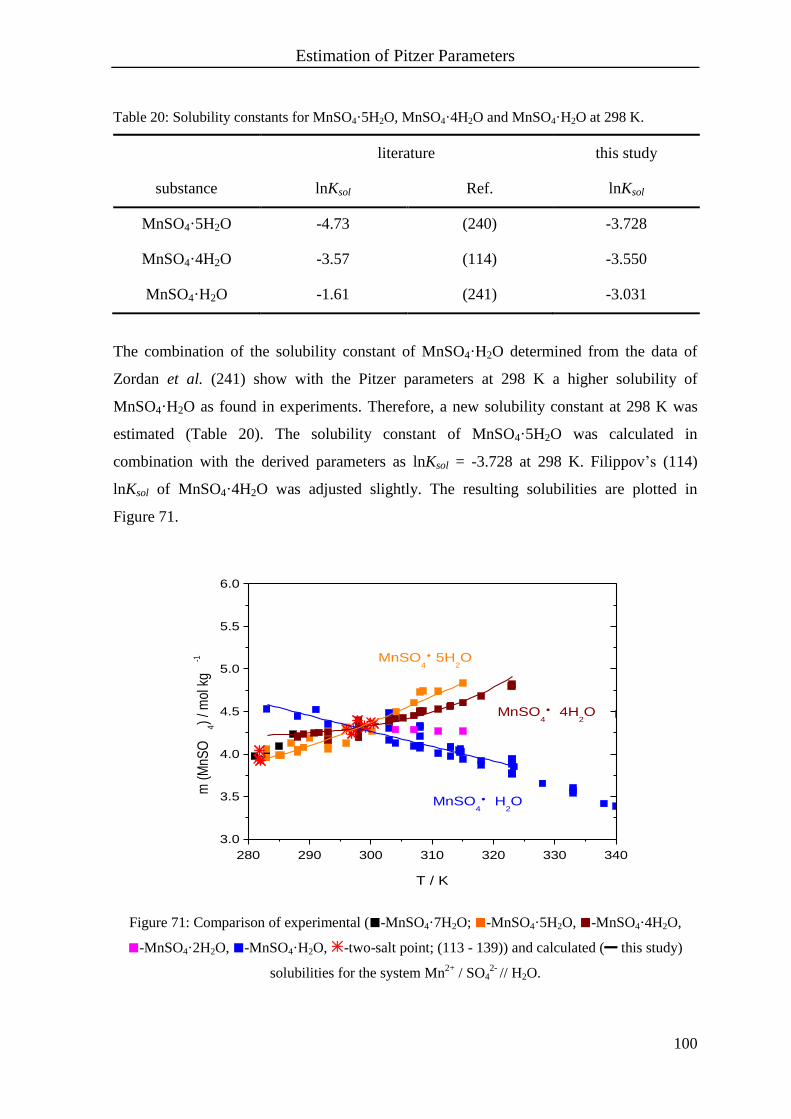
Estimation of Pitzer Parameters
100
Table 20: Solubility constants for MnSO4·5H2O, MnSO4·4H2O and MnSO4·H2O at 298 K.
literature this study
substance lnKsol Ref. lnKsol
MnSO4·5H2O -4.73 (240) -3.728
MnSO4·4H2O -3.57 (114) -3.550
MnSO4·H2O -1.61 (241) -3.031
The combination of the solubility constant of MnSO4·H2O determined from the data of
Zordan et al. (241) show with the Pitzer parameters at 298 K a higher solubility of
MnSO4·H2O as found in experiments. Therefore, a new solubility constant at 298 K was
estimated (Table 20). The solubility constant of MnSO4·5H2O was calculated in
combination with the derived parameters as lnKsol = -3.728 at 298 K. Filippov’s (114)
lnKsol of MnSO4·4H2O was adjusted slightly. The resulting solubilities are plotted in
Figure 71.
280 290 300 310 320 330 340
3.0
3.5
4.0
4.5
5.0
5.5
6.0
MnSO4
4H2O
MnSO4
H2O
MnSO4
5H2O
m (
MnS
O4)
/ mol
kg
-1
T / K
Figure 71: Comparison of experimental (-MnSO4·7H2O; -MnSO4·5H2O, -MnSO4·4H2O,
-MnSO4·2H2O, -MnSO4·H2O, -two-salt point; (113 - 139)) and calculated ( this study)
solubilities for the system Mn2+
/ SO42-
// H2O.

Estimation of Pitzer Parameters
101
In the system Co2+
/ SO42-
// H2O, new binary parameters are provided in this work. Hence,
the solubility constants of CoSO4·7H2O (242, 244) had to be adjusted to the new
parameters at 298 K.
Table 21: Solubility constants for CoSO4·7H2O and CoSO4·6H2O at 298 K.
literature this study
substance lnKsol Ref. lnKsol
CoSO4·7H2O -5.04 (242) -5.400
-5.028 (244)
CoSO4·6H2O -5.509 (240) -5.065
The solubility constant of CoSO4·6H2O calculated from the NBS tables (240) was fitted
also to the binary parameters and the experimental solubility data.
With the temperature-dependent parameters and the solubility constants of CoSO4·7H2O
and CoSO4·6H2O, the solubility was calculated in the system (Figure 72).
280 290 300 310 320 330 340
1.5
2.0
2.5
3.0
3.5
4.0
4.5
CoSO4
6H2O
CoSO4
7H2O
m (
CoS
O4)
/ mol
kg
-1
T / K
Figure 72: Comparison of experimental (-CoSO4·7H2O, -CoSO4·6H2O, -CoSO4·H2O, -two-
salt point; (97, 140 - 166)) and calculated ( this study) solubilities for the
system Co2+
/ SO42-
// H2O.

Estimation of Pitzer Parameters
102
Different solubility constants for NiSO4·7H2O were published at 298 K (Table 22). All of
them refer to the parameter set of Pitzer et al. (230).
Table 22: Solubility constants for NiSO4·7H2O and -NiSO4·6H2O at 298 K.
literature this study
substance lnKsol Ref. lnKsol
NiSO4·7H2O -5.07 (35) -5.208
-5.08 (245)
-NiSO4·6H2O -4.722 (240) -5.076
Because El Guendouzi’s (233) parameters showed a smaller deviation of the calculated
osmotic coefficient from the experimental data, their parameter set was employed in this
study. Thus, the provided solubility constants were adjusted slightly. The same was
performed with the solubility constant for -NiSO4·6H2O, determined from the NBS tables
(240). Calculated solubilities are shown in Figure 73.
280 290 300 310 320 330 340
1.5
2.0
2.5
3.0
3.5
4.0
- NiSO4
6H2O
NiSO4
7H2O
m (
NiS
O4)
/ mol
kg
-1
T / K
Figure 73: Comparison of experimental (-NiSO4·7H2O, --NiSO4·6H2O, -β-NiSO4·6H2O,
-two-salt point; (167 - 180)) and calculated ( this study) solubilities for the
system Ni2+
/ SO42-
// H2O.
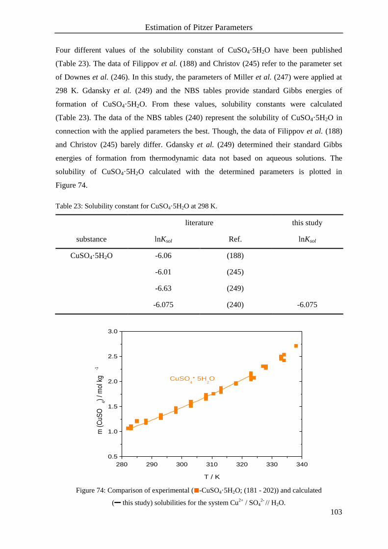
Estimation of Pitzer Parameters
103
Four different values of the solubility constant of CuSO4·5H2O have been published
(Table 23). The data of Filippov et al. (188) and Christov (245) refer to the parameter set
of Downes et al. (246). In this study, the parameters of Miller et al. (247) were applied at
298 K. Gdansky et al. (249) and the NBS tables provide standard Gibbs energies of
formation of CuSO4·5H2O. From these values, solubility constants were calculated
(Table 23). The data of the NBS tables (240) represent the solubility of CuSO4·5H2O in
connection with the applied parameters the best. Though, the data of Filippov et al. (188)
and Christov (245) barely differ. Gdansky et al. (249) determined their standard Gibbs
energies of formation from thermodynamic data not based on aqueous solutions. The
solubility of CuSO4·5H2O calculated with the determined parameters is plotted in
Figure 74.
Table 23: Solubility constant for CuSO4·5H2O at 298 K.
literature this study
substance lnKsol Ref. lnKsol
CuSO4·5H2O -6.06 (188)
-6.01 (245)
-6.63 (249)
-6.075 (240) -6.075
280 290 300 310 320 330 340
0.5
1.0
1.5
2.0
2.5
3.0
CuSO4
5H2O
m (
CuS
O4)
/ mol
kg
-1
T / K
Figure 74: Comparison of experimental (-CuSO4·5H2O; (181 - 202)) and calculated
( this study) solubilities for the system Cu2+
/ SO42-
// H2O.
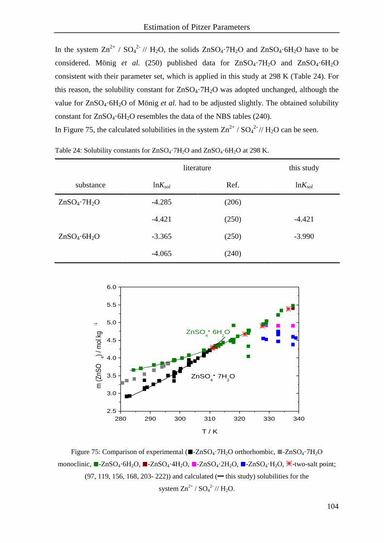
Estimation of Pitzer Parameters
104
In the system Zn2+
/ SO42-
// H2O, the solids ZnSO4·7H2O and ZnSO4·6H2O have to be
considered. Mönig et al. (250) published data for ZnSO4·7H2O and ZnSO4·6H2O
consistent with their parameter set, which is applied in this study at 298 K (Table 24). For
this reason, the solubility constant for ZnSO4·7H2O was adopted unchanged, although the
value for ZnSO4·6H2O of Mönig et al. had to be adjusted slightly. The obtained solubility
constant for ZnSO4·6H2O resembles the data of the NBS tables (240).
In Figure 75, the calculated solubilities in the system Zn2+
/ SO42-
// H2O can be seen.
Table 24: Solubility constants for ZnSO4·7H2O and ZnSO4·6H2O at 298 K.
literature this study
substance lnKsol Ref. lnKsol
ZnSO4·7H2O -4.285 (206)
-4.421 (250) -4.421
ZnSO4·6H2O -3.365 (250) -3.990
-4.065 (240)
280 290 300 310 320 330 340
2.5
3.0
3.5
4.0
4.5
5.0
5.5
6.0
ZnSO4
7H2O
ZnSO4
6H2O
m (
ZnS
O4)
/ mol
kg
-1
T / K
Figure 75: Comparison of experimental (-ZnSO4·7H2O orthorhombic, -ZnSO4·7H2O
monoclinic, -ZnSO4·6H2O, -ZnSO4·4H2O, -ZnSO4·2H2O, -ZnSO4·H2O, -two-salt point;
(97, 119, 156, 168, 203- 222)) and calculated ( this study) solubilities for the
system Zn2+
/ SO42-
// H2O.
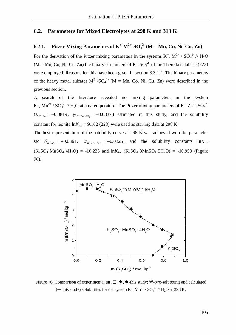
Estimation of Pitzer Parameters
105
6.2. Parameters for Mixed Electrolytes at 298 K and 313 K
6.2.1. Pitzer Mixing Parameters of K+-M
2+-SO4
2- (M = Mn, Co, Ni, Cu, Zn)
For the derivation of the Pitzer mixing parameters in the systems K+, M
2+ / SO4
2- // H2O
(M = Mn, Co, Ni, Cu, Zn) the binary parameters of K+-SO4
2- of the Thereda database (223)
were employed. Reasons for this have been given in section 3.3.1.2. The binary parameters
of the heavy metal sulfates M2+
-SO42-
(M = Mn, Co, Ni, Cu, Zn) were described in the
previous section.
A search of the literature revealed no mixing parameters in the system
K+, Mn
2+ / SO4
2- // H2O at any temperature. The Pitzer mixing parameters of K
+-Zn
2+-SO4
2-
( 0819.0ZnK , 0337.04
SOZnK ) estimated in this study, and the solubility
constant for leonite lnKsol = 9.162 (223) were used as starting data at 298 K.
The best representation of the solubility curve at 298 K was achieved with the parameter
set 0361.0MnK , 0325.04
SOMnK , and the solubility constants lnKsol
(K2SO4·MnSO4·4H2O) = -10.223 and lnKsol (K2SO4·3MnSO4·5H2O) = -16.959 (Figure
76).
0.0 0.2 0.4 0.6 0.8 1.0
0
1
2
3
4
5
K2SO
4
K2SO
4
MnSO4
4H2O
MnSO4
H2O
K2SO
4
3MnSO4
5H2O
m (
MnS
O4)
/ mol
kg
-1
m (K2SO
4) / mol kg
-1
Figure 76: Comparison of experimental (, , , -this study; -two-salt point) and calculated
( this study) solubilities for the system K+, Mn
2+ / SO4
2- // H2O at 298 K.

Estimation of Pitzer Parameters
106
Using the estimated parameters at 298 K as starting data, the parameters at 313 K were
determined as 0241.0MnK , 0180.04
SOMnK , and the solubility constants
lnKsol (K2SO4·2MnSO4) = -14.673 and lnKsol (K2SO4·MnSO4·1.5H2O) = -19.725
(Figure 77).
0.0 0.2 0.4 0.6 0.8 1.0
0.0
0.5
1.0
1.5
2.0
2.5
3.0
3.5
4.0
4.5
K2SO
4
2MnSO4
K2SO
4
K2SO
4
MnSO4
1.5H2O
MnSO4
H2O
m (
MnS
O4)
/ mol
kg
-1
m (K2SO
4) / mol kg
-1
Figure 77: Comparison of experimental (, , , -this study; -two-salt point) and calculated
( this study) solubilities for the system K+, Mn
2+ / SO4
2- // H2O at 313 K.
As discussed in section 4.2.2, Filippov et al. published two data sets of solubilities for the
system K+, Co
2+ / SO4
2- // H2O. One was determined experimentally (41) and the other
calculated with Pitzer’s equation (35). Solubility data calculated by Filippov et al.
resemble the values of Caven et al. (33). In this study, the parameters reflect Filippov’s
experimental data (section 3.3.2.1).
Filippov et al. (35) published parameters regarding the ion interaction of K+-Co
2+-SO4
2-,
and a solubility constant for K2SO4·CoSO4·6H2O at 298 K ( 127.0CoK ,
04 SOCoK , lnKsol = -11.97). Due to the re-determination of the binary parameters of
CoSO4, the mixing parameters and the solubility constant of K2SO4·CoSO4·6H2O had to
be adjusted ( 0722.0CoK , 0241.04
SOMK , lnKsol = -12.508). However, since the
binary and mixing parameters of Filippov et al. were applied for calculations, the
experimental data can not be reproduced. This was noticed also for the other heavy metal-
containing systems of this study.
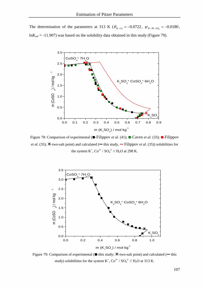
Estimation of Pitzer Parameters
107
The determination of the parameters at 313 K ( 0722.0CoK , 0180.04
SOMK ,
lnKsol = -11.907) was based on the solubility data obtained in this study (Figure 79).
0.0 0.1 0.2 0.3 0.4 0.5 0.6 0.7 0.8 0.9
0.0
0.5
1.0
1.5
2.0
2.5
3.0
K2SO
4
K2SO
4
CoSO4
6H2O
CoSO4
7H2O
m (
CoS
O4)
/ mol
kg
-1
m (K2SO
4) / mol kg
-1
Figure 78: Comparison of experimental (-Filippov et al. (41); -Caven et al. (33); -Filippov
et al. (35); -two-salt point) and calculated ( this study, Filippov et al. (35)) solubilities for
the system K+, Co
2+ / SO4
2- // H2O at 298 K.
0.0 0.2 0.4 0.6 0.8 1.0
0.0
0.5
1.0
1.5
2.0
2.5
3.0
3.5
K2SO
4
K2SO
4
CoSO4
6H2O
CoSO4
7H2O
m (
CoS
O4)
/ mol
kg
-1
m (K2SO
4) / mol kg
-1
Figure 79: Comparison of experimental (-this study; -two-salt point) and calculated ( this
study) solubilities for the system K+, Co
2+ / SO4
2- // H2O at 313 K.

Estimation of Pitzer Parameters
108
Three different sets of Pitzer mixing parameters for K+ - Ni
2+ -SO4
2- and solubility
constants for K2SO4·NiSO4·6H2O have been published, but only for 298 K. The
parameters were checked at the crystallization branch of K2SO4·NiSO4·6H2O at 298 K. It
can be seen that the parameter set of Bremer et al. (296) ( 01.0NiK ,
-0.061144 SONiK , lnKsol (K2SO4·NiSO4·6H2O) = -14.483) expresses the solubility the
best (Figure 80).
However, the parameters of Bremer et al. (296) are valid at 298 K, and they also reproduce
the solubilities at 313 K after slight adjustment of the solubility constant for
K2SO4·NiSO4·6H2O (lnKsol = -13.831) (Figure 81).
Figure 80: Comparison of experimental (-Filippov et al. (35); -two-salt point) and calculated
( Filippov et al. (35), Christov (244), Bremer et al. (296)) solubilities for the system
K+, Ni
2+ / SO4
2- // H2O at 298 K.
0.0 0.1 0.2 0.3 0.4 0.5 0.6 0.7 0.8
0.0
0.5
1.0
1.5
2.0
2.5
3.0
K2SO
4
K2SO
4
NiSO4
6H2O
NiSO4
7H2O
m (
NiS
O4)
/ m
ol k
g-1
m (K2SO
4) / mol kg
-1
0.3 0.4 0.5 0.6 0.7 0.80.00
0.05
0.10
0.15
K2SO
4
K2SO
4
NiSO4
6H2O
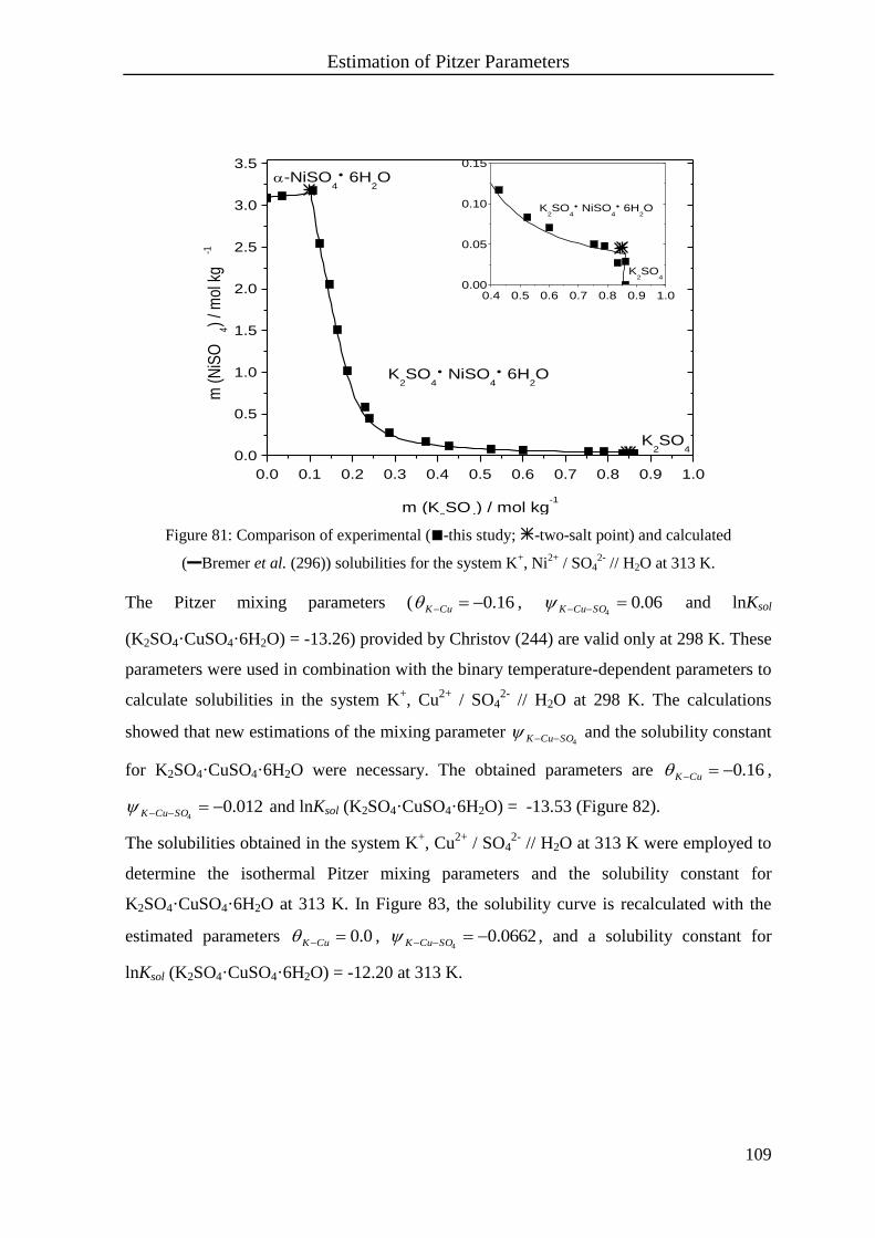
Estimation of Pitzer Parameters
109
Figure 81: Comparison of experimental (-this study; -two-salt point) and calculated
(Bremer et al. (296)) solubilities for the system K+, Ni
2+ / SO4
2- // H2O at 313 K.
The Pitzer mixing parameters ( 16.0CuK , 06.04 SOCuK and lnKsol
(K2SO4·CuSO4·6H2O) = -13.26) provided by Christov (244) are valid only at 298 K. These
parameters were used in combination with the binary temperature-dependent parameters to
calculate solubilities in the system K+, Cu
2+ / SO4
2- // H2O at 298 K. The calculations
showed that new estimations of the mixing parameter 4SOCuK and the solubility constant
for K2SO4·CuSO4·6H2O were necessary. The obtained parameters are 16.0CuK ,
012.04
SOCuK and lnKsol (K2SO4·CuSO4·6H2O) = -13.53 (Figure 82).
The solubilities obtained in the system K+, Cu
2+ / SO4
2- // H2O at 313 K were employed to
determine the isothermal Pitzer mixing parameters and the solubility constant for
K2SO4·CuSO4·6H2O at 313 K. In Figure 83, the solubility curve is recalculated with the
estimated parameters 0.0CuK , 0662.04
SOCuK , and a solubility constant for
lnKsol (K2SO4·CuSO4·6H2O) = -12.20 at 313 K.
0.0 0.1 0.2 0.3 0.4 0.5 0.6 0.7 0.8 0.9 1.0
0.0
0.5
1.0
1.5
2.0
2.5
3.0
3.5
K2SO
4
K2SO
4
NiSO4
6H2O
-NiSO4
6H2O
m (
NiS
O4)
/ mol
kg
-1
m (K2SO
4) / mol kg
-1
0.4 0.5 0.6 0.7 0.8 0.9 1.00.00
0.05
0.10
0.15
K2SO
4
K2SO
4
NiSO4
6H2O
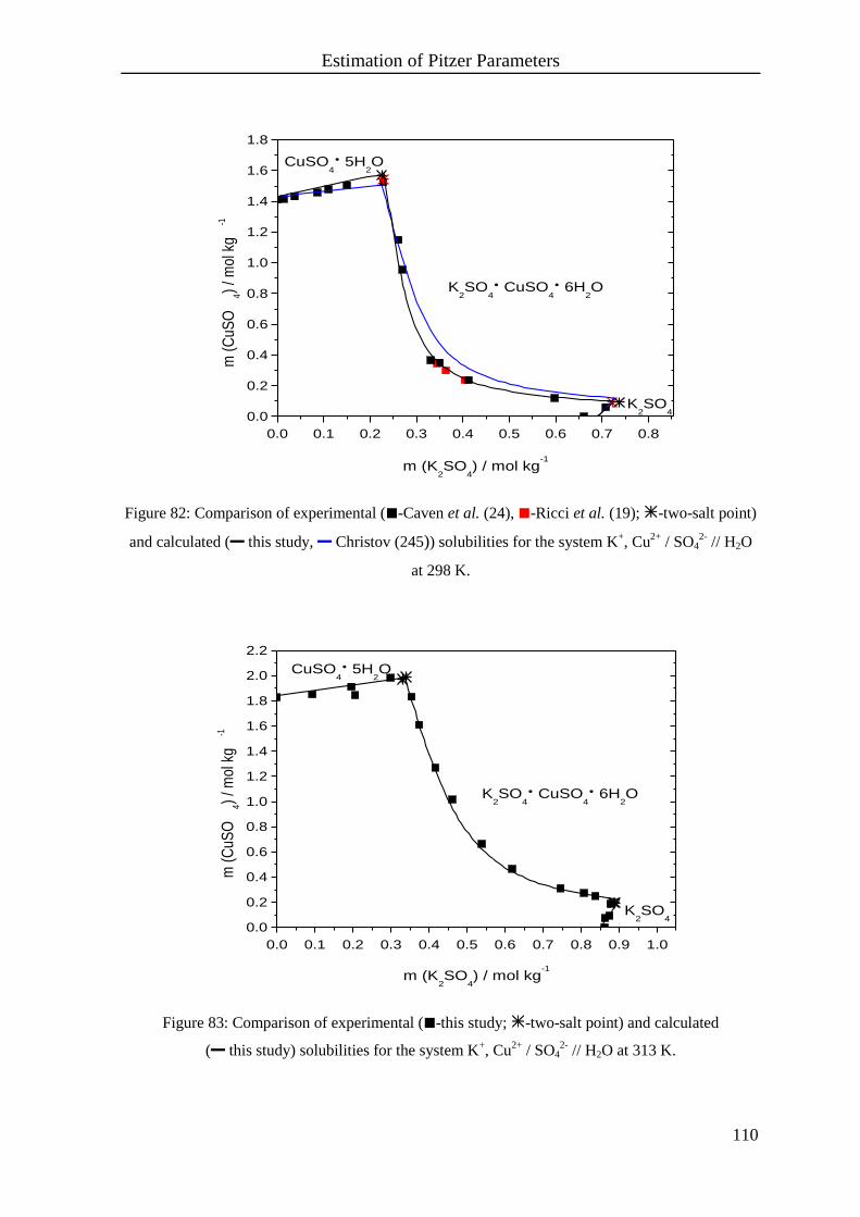
Estimation of Pitzer Parameters
110
0.0 0.1 0.2 0.3 0.4 0.5 0.6 0.7 0.8
0.0
0.2
0.4
0.6
0.8
1.0
1.2
1.4
1.6
1.8
CuSO4
5H2O
K2SO
4
K2SO
4
CuSO4
6H2O
m (
CuS
O4)
/ mol
kg
-1
m (K2SO
4) / mol kg
-1
Figure 82: Comparison of experimental (-Caven et al. (24), -Ricci et al. (19); -two-salt point)
and calculated ( this study, Christov (245)) solubilities for the system K+, Cu
2+ / SO4
2- // H2O
at 298 K.
0.0 0.1 0.2 0.3 0.4 0.5 0.6 0.7 0.8 0.9 1.0
0.0
0.2
0.4
0.6
0.8
1.0
1.2
1.4
1.6
1.8
2.0
2.2
K2SO
4
K2SO
4
CuSO4
6H2O
CuSO4
5H2O
m (
CuS
O4)
/ mol
kg
-1
m (K2SO
4) / mol kg
-1
Figure 83: Comparison of experimental (-this study; -two-salt point) and calculated
( this study) solubilities for the system K+, Cu
2+ / SO4
2- // H2O at 313 K.

Estimation of Pitzer Parameters
111
In the system K+, Zn
2+ / SO4
2- // H2O, Pitzer mixing parameters are provided by Filippov et
al. (45) and Mönig (250) at 298 K. The binary temperature-dependent parameters and the
mixing parameters from the literature were used to recalculate the solubilities at 298 K.
Four different data sets are published at 298 K (23, 38, 45, 295) (section 3.3.2.1). In this
study, the solubility data of Filippov et al. (45) and Lipscomb et al. (295) were taken to
describe the true solubility in the system.
0.0 0.1 0.2 0.3 0.4 0.5 0.6 0.7 0.8
0.0
0.5
1.0
1.5
2.0
2.5
3.0
3.5
4.0
K2SO
4
ZnSO4
7H2O
K2SO
4
ZnSO4
6H2O
m (
ZnS
O4)
/ mol
kg
-1
m (K2SO
4) / mol kg
-1
Figure 84: Comparison of experimental (-Filippov et al. (45), -Lipscomb et al. (295);
-two-salt point) and calculated ( this study, Filippov et al. (45), Mönig et al. (250))
solubilities for the system K+, Zn
2+ / SO4
2- // H2O at 298 K.
From Figure 84 it can be seen that a slight adjustment of the parameters and the solubility
constant for K2SO4·ZnSO4·6H2O is required. The parameter 0819.0ZnK was adopted
from Filippov et al. (45) and 4SOZnK changed to 0337.0
4 SOZnK . The solubility
constant was lnKsol (K2SO4·ZnSO4·6H2O) = -13.05 at 298 K.
Since no mixing parameters are published for 313 K, their estimation was based on the
parameters at 298 K. The resulting parameters for the solubility curve at 313 K are
0986.0ZnK , 0120.04
SOZnK and a lnKsol of K2SO4·ZnSO4·6H2O of -12.33
(Figure 85).
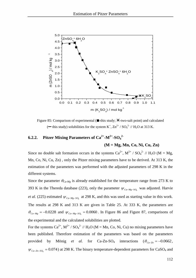
Estimation of Pitzer Parameters
112
0.0 0.1 0.2 0.3 0.4 0.5 0.6 0.7 0.8 0.9 1.0 1.1
0.0
0.5
1.0
1.5
2.0
2.5
3.0
3.5
4.0
4.5
5.0
K2SO
4
ZnSO4
6H2O
K2SO
4
ZnSO4
6H2O
m (
ZnS
O4)
/ mol
kg
-1
m (K2SO
4) / mol kg
-1
Figure 85: Comparison of experimental (-this study; -two-salt point) and calculated
( this study) solubilities for the system K+, Zn
2+ / SO4
2- // H2O at 313 K.
6.2.2. Pitzer Mixing Parameters of Ca2+
-M2+
-SO42-
(M = Mg, Mn, Co, Ni, Cu, Zn)
Since no double salt formation occurs in the systems Ca2+
, M2+
/ SO42-
// H2O (M = Mg,
Mn, Co, Ni, Cu, Zn) , only the Pitzer mixing parameters have to be derived. At 313 K, the
estimation of the parameters was performed with the adjusted parameters of 298 K in the
different systems.
Since the parameter Ca-Mg is already established for the temperature range from 273 K to
393 K in the Thereda database (223), only the parameter 4SOMgCa was adjusted. Harvie
et al. (225) estimated 4SOMgCa at 298 K, and this was used as starting value in this work.
The results at 298 K and 313 K are given in Table 25. At 333 K, the parameters are
0228.0MgCa and 0060.04 SOMgCa . In Figure 86 and Figure 87, comparisons of
the experimental and the calculated solubilities are plotted.
For the systems Ca2+
, M2+
/ SO42-
// H2O (M = Mn, Co, Ni, Cu) no mixing parameters have
been published. Therefore estimation of the parameters was based on the parameters
provided by Mönig et al. for Ca-Zn-SO4 interactions ( 0662.0ZnCa ,
074.04 SOZnCa ) at 298 K. The binary temperature-dependent parameters for CaSO4 and

Estimation of Pitzer Parameters
113
the appropriate heavy metal sulfate were as determined previously (section 6.1.2).
Obtained parameters are summarized in Table 25. Figure 86 shows the calculated
solubilities in the systems Ca2+
, M2+
/ SO42-
// H2O (M = Mg, Mn, Co, Ni, Cu) at 298 K
and 313 K, using the parameters in Table 25.
0.0
0.5
1.0
1.5
2.0
0 1 2 3 40.0
0.5
1.0
1.5
2.0
0 1 2 3 4
0.0
0.5
1.0
1.5
2.0
Co
Mn
Ni
102 m
(C
aSO
4)
/ m
ol k
g-1
Cu
m (MSO4 (M = Mg, Mn, Co, Ni, Cu, Zn)) / mol kg
-1
Zn
Mg
Figure 86: Comparison of experimental (-this study at 298 K, -this study at 313 K; -two-salt
point) and calculated ( this study at 298 K, this study at 313 K) solubilities for the system
Ca2+
, M2+
/ SO42-
// H2O (M = Mg, Mn, Co, Ni, Cu, Zn) at 298 K and 313 K.

Estimation of Pitzer Parameters
114
0.0 0.5 1.0 1.5 2.0 2.5 3.0 3.5 4.0 4.5 5.0
0.0
0.2
0.4
0.6
0.8
1.0
1.2
1.4
1.6
1.8
CaSO4
MgS
O4
6
H2O
102 m
(C
aSO
4)
/ mol
kg
-1
m (MgSO4) / mol kg
-1
Figure 87: Comparison of experimental (-this study; -two-salt point) and calculated
( this study) solubilities for the system Ca2+
, Mg2+
/ SO42-
// H2O at 333 K.
Harvie et al. (225) used the solubility data of Cameron et al. (298) to estimate their
parameters (Figure 88). In this work it was shown, that the data of Cameron et al. are not
precise (section 4.3.2). Therefore, a new value had to be derived for 4SOMgCa at 298 K.
0.0 0.5 1.0 1.5 2.0 2.5 3.0 3.5
0.0
0.2
0.4
0.6
0.8
1.0
1.2
1.4
1.6
MgS
O4
7
H2O
CaSO4
2H2O
102 m
(C
aSO
4)
/ mol
kg
-1
m (MgSO4) / mol kg
-1
Figure 88: Comparison of experimental (-this study, -Cameron et al. (298); -two-salt point)
and calculated ( this study, Harvie et al. (225)) solubilities for the system
Ca2+
, Mg2+
/ SO42-
// H2O at 298 K.

Estimation of Pitzer Parameters
115
In the system Ca2+
, Zn2+
/ SO42-
// H2O, adjustment of the parameters of Mönig et al. was
also necessary. This is due to the more precise solubility data determined in this study.
0.0 0.5 1.0 1.5 2.0 2.5 3.0 3.5 4.0
0.0
0.2
0.4
0.6
0.8
1.0
1.2
1.4
1.6
1.8
ZnS
O4
7
H2O
CaSO4
2H2O
102 m
(C
aSO
4)
/ mol
kg
-1
m (ZnSO4) / mol kg
-1
Figure 89: Comparison of experimental (-this study; -two-salt point) and calculated ( this
study, Mönig et al. (250)) solubilities for the system Ca2+
, Zn2+
/ SO42-
// H2O at 298 K.
Table 25: Pitzer mixing parameters MCa and 4SOMCa at 298 K and 313 K.
298 K 313 K
M MCa
4SOMCa MCa
4SOMCa
Mg -0.0180 -0.0120 -0.0201 0.0084
Mn -0.0457 -0.00842 -0.0241 0.0144
Co -0.0361 -0.0144 -0.0300 0
Ni -0.0120 -0.00601 -0.0180 0
Cu -0.0457 0 -0.0241 -0.0192
Zn -0.0541 0.00722 -0.0541 0.0180

Estimation of Solubility Constants of Polyhalite and its Analogues
116
7. Estimation of Solubility Constants of Polyhalite and its
Analogues, K2SO4·MSO4·2CaSO4·2H2O
(M = Mg, Mn, Co, Ni, Cu, Zn)
To derive the solubility constant of a salt, the activities of the ions and of water involved
are necessary (section 3.2). In the case of polyhalite (Ph), the solubility constant is written
as follows.
2422
4 WSOCaMKsol aaaaaPhK . [60]
Adding iii ma and writing the equation in the logarithmic form, it results in the
following expression.
)ln(2)ln(4)ln(2)ln()ln(2ln44 WSOSOCaCaMMKKsol ammmmPhK [61]
The molalities of the ions were determined with solid-liquid equilibrium experiments. The
required activity coefficients of the ions and the activity of water were calculated with
Pitzer’s equation (section 3.2.1) using the parameters of the Thereda database (223) and
the parameters obtained in this work (Chapter 6). Phase equilibrium calculations were
executed with chemsage (327).
The System K+, Mg
2+, Ca
2+ / SO4
2- // H2O
Various studies of solubility equilibria of polyhalite have been published. An et al. (328)
examined the time polyhalites take to reach equilibrium, when they dissolve. Accordingly,
a slightly chloridic polyhalite was dissolved in water at 298 K, 323 K, and 348 K, as well
as in 5 % and 20 % CaCl2 solutions at 298 K. At different time intervals they sampled the
solution and analyzed for the cations potassium, magnesium and calcium.
In pure water, equilibrium was reached after 100 h to 150 h without significant influence of
temperature. It needs to be noted that An et al. do not give numeric data and the plot of the
calcium concentration versus time is not informative about the equilibrium. In the case of
the dissolution of polyhalite in 5 % and 10 % CaCl2 solutions, equilibration times of
around 700 h were needed. In this case, the plots are evident of the equilibrium.
To date, solid-liquid equilibrium experiments involving polyhalite were performed by
dissolving this salt in different concentrated solutions.
In the quaternary system K+, Mg
2+, Ca
2+ / SO4
2- // H2O, first experiments were performed
by Basch (303) at 298 K, and these were published also by van’t Hoff (1) later. The data
were rejected by Klooster (276) and D’Ans (307) some years later, with the explanation
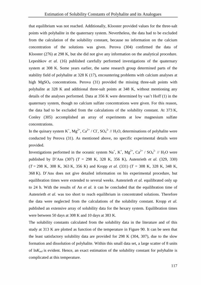
Estimation of Solubility Constants of Polyhalite and its Analogues
117
that equilibrium was not reached. Additionally, Klooster provided values for the three-salt
points with polyhalite in the quaternary system. Nevertheless, the data had to be excluded
from the calculation of the solubility constant, because no information on the calcium
concentration of the solutions was given. Perova (304) confirmed the data of
Klooster (276) at 298 K, but she did not give any information on the analytical procedure.
Lepeshkov et al. (16) published carefully performed investigations of the quaternary
system at 308 K. Some years earlier, the same research group determined parts of the
stability field of polyhalite at 328 K (17), encountering problems with calcium analyses at
high MgSO4 concentrations. Perova (31) provided the missing three-salt points with
polyhalite at 328 K and additional three-salt points at 348 K, without mentioning any
details of the analyses performed. Data at 356 K were determined by van’t Hoff (1) in the
quaternary system, though no calcium sulfate concentrations were given. For this reason,
the data had to be excluded from the calculations of the solubility constant. At 373 K,
Conley (305) accomplished an array of experiments at low magnesium sulfate
concentrations.
In the quinary system K+, Mg
2+, Ca
2+ / Cl
-, SO4
2- // H2O, determinations of polyhalite were
conducted by Perova (31). As mentioned above, no specific experimental details were
provided.
Investigations performed in the oceanic system Na+, K
+, Mg
2+, Ca
2+ / SO4
2- // H2O were
published by D’Ans (307) (T = 298 K, 328 K, 356 K), Autenrieth et al. (329, 330)
(T = 298 K, 308 K, 363 K, 356 K) and Kropp et al. (331) (T = 308 K, 328 K, 348 K,
368 K). D’Ans does not give detailed information on his experimental procedure, but
equilibration times were extended to several weeks. Autenrieth et al. equilibrated only up
to 24 h. With the results of An et al. it can be concluded that the equilibration time of
Autenrieth et al. was too short to reach equilibrium in concentrated solutions. Therefore
the data were neglected from the calculations of the solubility constant. Kropp et al.
published an extensive array of solubility data for the hexary system. Equilibration times
were between 50 days at 308 K and 10 days at 383 K.
The solubility constants calculated from the solubility data in the literature and of this
study at 313 K are plotted as function of the temperature in Figure 90. It can be seen that
the least satisfactory solubility data are provided for 298 K (304, 307), due to the slow
formation and dissolution of polyhalite. Within this small data set, a large scatter of 8 units
of lnKsol is evident. Hence, an exact estimation of the solubility constant for polyhalite is
complicated at this temperature.

Estimation of Solubility Constants of Polyhalite and its Analogues
118
260 280 300 320 340 360 380
-50
-45
-40
-35
-30
-25
ln K
sol
T / K
Figure 90: Solubility constants for polyhalite calculated from solubility data with Pitzer’s equation
and the parameters of the Thereda database (223); -D’Ans (307), -Perova (304),
-Kropp et al. (331), -Lepeshkov et al. (16), -this study, -Bodaleva et al. (17), -Conley et
al. (305), -Risacher et al. (308); color code of the temperatures: -298K, -308 K, -313 K,
-328 K, -348 K, -356 K, -368 K, -373K, -383 K.
At 308 K, the values calculated from the solubility data of Lepeshkov et al. (16) and of
Kropp et al. (331) coincide within 5.5 units of lnKsol. The same can be seen for the data of
Bodaleva et al. (17) and Kropp et al. at 328 K. The solubility constants calculated from the
solubility data of D’Ans (307) of 328 K show a somewhat larger variance. At 356 K, the
values calculated from D’Ans’s data fit with the solubility constants of Kropp’s (331) data.
From Figure 90, it is also obvious that the solubility constants calculated from the data of
Perova (304) are systematically higher than those of Kropp et al. and Bodaleva et al.
Additionally, the solubility constants of Risacher et al. (308) at different temperatures are
plotted in Figure 90. It is noted that the slope of lnKsol is smoother than a line connecting
the mean values of Kropp et al.
Risacher et al. based their calculations on the solubility constant at 298 K and the
temperature-dependence of the entropy of the formation reactions of polyhalite between
273 K and 573 K (section 3.3.4.2).
Hence the data of Risacher et al. give evidence for the trend of the dependence of the
solubility constant for polyhalite on temperature. Accordingly, the data of
Conley et al. (305) appear more reliable. This follows also from the equilibration times.
Kropp et al. equilibrated their solutions for 20 days at 348 K, and 10 days at 368 K and

Estimation of Solubility Constants of Polyhalite and its Analogues
119
383 K. Conley et al. used equilibration times of between 15 days to 50 days, mostly around
30 days, at 373 K. Furthermore, Kropp et al. examined the stability field of polyhalite in a
higher system than Conley et al., which leads to a higher uncertainty for any data point,
due to the increased number of chemical analyses performed and the influence of the
increasing number of Pitzer parameters needed to describe the system.
Since the calculated solubility constants at 298 K scatter considerably, the value has to be
determined from other data. For this reason, the mean solubility constant at 313 K
(lnKsol = -33.31) calculated from the data of this study was extrapolated to 298 K using the
enthalpy of dissolution of polyhalite as given below.
RT
H
T
K msolsol
ln [62]
Within a small temperature range, it can be approximated that the enthalpy of dissolution
at infinite dilution does not depend on the temperature.
The calculated value at 298 K is plotted in Figure 91 and summarized with the solubility
constants of the heavy metal-containing polyhalites in Table 26. Comparison of the value
of Harvie et al. (225) (lnKsol = -31.65) and the calculated value for the solubility
experiments at 313 K (lnKsol = -32.58) shows a difference of one unit in lnKsol. Harvie et
al. stated that they estimated their value from the data of D’Ans (307) and Perova (304),
although the solubility constants calculated from these solubility data are significantly
higher.
Now, the temperature-dependence of the solubility constant of polyhalite can be
determined from 298 K to 373 K using the calculated solubility constants at the different
temperatures.
Therefore, the obtained solubility constants were fitted to the quadratic
lnKsol = B + DT + ET2, neglecting the data of Perova (304), D’Ans (307) and
Kropp et al. (331) above 328 K (Figure 92). The value of Harvie et al. (225) was not taken
into account in favor of the newly determined solubility constant for polyhalite at 298 K.
This constant at 298 K was weighted at 1.0, while the other data points at higher
temperatures were given a weight of 0.01. The data obtained from the quadratic plot are
B = -82.176742, D = 3.61193944·10-1
, and E = -6.530600·10-4
.
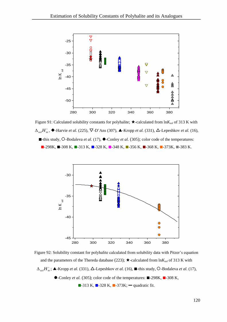
Estimation of Solubility Constants of Polyhalite and its Analogues
120
280 300 320 340 360 380
-50
-45
-40
-35
-30
-25
ln K
sol
T / K
Figure 91: Calculated solubility constants for polyhalite; -calculated from lnKsol of 313 K with
msolH , -Harvie et al. (225), -D’Ans (307), -Kropp et al. (331), -Lepeshkov et al. (16),
-this study, -Bodaleva et al. (17), -Conley et al. (305); color code of the temperatures:
-298K, -308 K, -313 K, -328 K, -348 K, -356 K, -368 K, -373K, -383 K.
280 300 320 340 360 380
-45
-40
-35
-30
ln K
sol
T / K
Figure 92: Solubility constant for polyhalite calculated from solubility data with Pitzer’s equation
and the parameters of the Thereda database (223); -calculated from lnKsol of 313 K with
msolH ; -Kropp et al. (331), -Lepeshkov et al. (16), -this study, -Bodaleva et al. (17),
-Conley et al. (305); color code of the temperatures: -298K, -308 K,
-313 K, -328 K, -373K; quadratic fit.
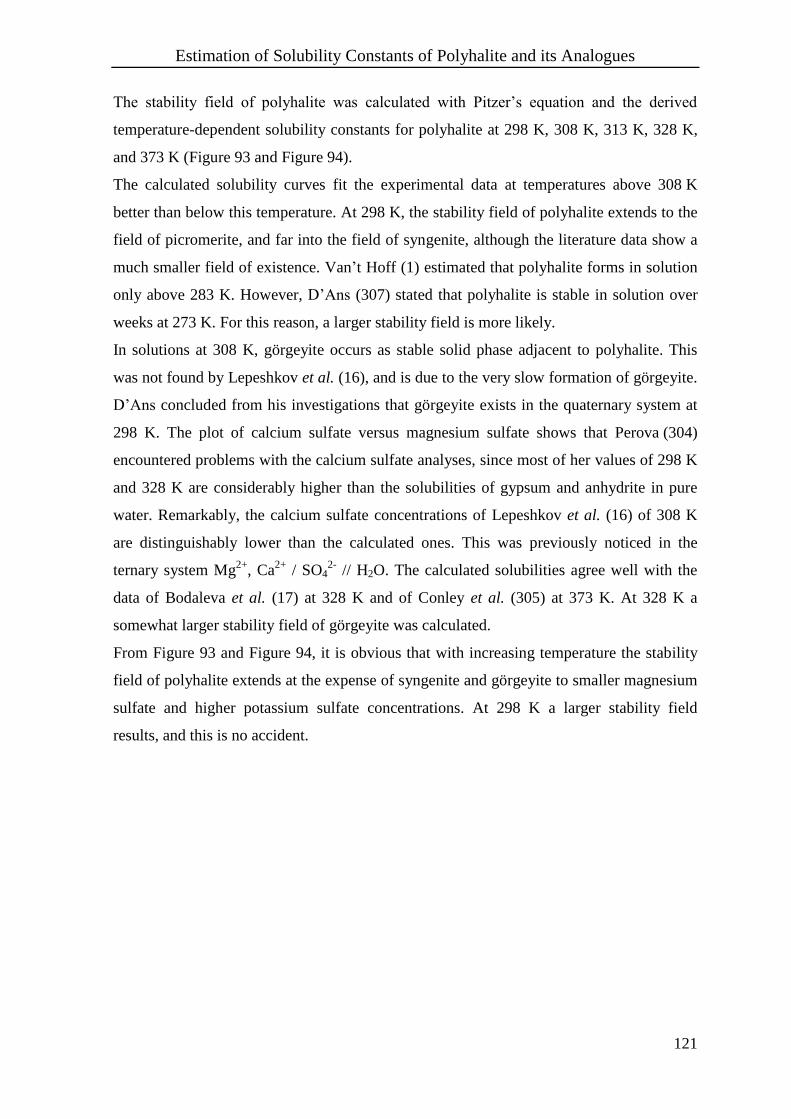
Estimation of Solubility Constants of Polyhalite and its Analogues
121
The stability field of polyhalite was calculated with Pitzer’s equation and the derived
temperature-dependent solubility constants for polyhalite at 298 K, 308 K, 313 K, 328 K,
and 373 K (Figure 93 and Figure 94).
The calculated solubility curves fit the experimental data at temperatures above 308 K
better than below this temperature. At 298 K, the stability field of polyhalite extends to the
field of picromerite, and far into the field of syngenite, although the literature data show a
much smaller field of existence. Van’t Hoff (1) estimated that polyhalite forms in solution
only above 283 K. However, D’Ans (307) stated that polyhalite is stable in solution over
weeks at 273 K. For this reason, a larger stability field is more likely.
In solutions at 308 K, görgeyite occurs as stable solid phase adjacent to polyhalite. This
was not found by Lepeshkov et al. (16), and is due to the very slow formation of görgeyite.
D’Ans concluded from his investigations that görgeyite exists in the quaternary system at
298 K. The plot of calcium sulfate versus magnesium sulfate shows that Perova (304)
encountered problems with the calcium sulfate analyses, since most of her values of 298 K
and 328 K are considerably higher than the solubilities of gypsum and anhydrite in pure
water. Remarkably, the calcium sulfate concentrations of Lepeshkov et al. (16) of 308 K
are distinguishably lower than the calculated ones. This was previously noticed in the
ternary system Mg2+
, Ca2+
/ SO42-
// H2O. The calculated solubilities agree well with the
data of Bodaleva et al. (17) at 328 K and of Conley et al. (305) at 373 K. At 328 K a
somewhat larger stability field of görgeyite was calculated.
From Figure 93 and Figure 94, it is obvious that with increasing temperature the stability
field of polyhalite extends at the expense of syngenite and görgeyite to smaller magnesium
sulfate and higher potassium sulfate concentrations. At 298 K a larger stability field
results, and this is no accident.

Estimation of Solubility Constants of Polyhalite and its Analogues
122
0.0
0.5
1.0
1.5
2.0
2.5
3.0
3.5
4.0
4.5
5.0
0.0
0.5
1.0
1.5
2.0
2.5
3.0
3.5
4.0
4.5
5.0
0.0 0.2 0.4 0.6 0.8 1.0 1.2 1.4 1.6
0.0
0.5
1.0
1.5
2.0
2.5
3.0
3.5
4.0
4.5
5.0 0.0 0.2 0.4 0.6 0.8 1.0 1.2 1.4 1.6
Ph
K2SO
4
CaS
O4
2H
2O
K2S
O4
CaS
O4
H2O
K2SO
4
MgSO4
6H2O
MgSO4
7H2O
m (
MgS
O4)
/ mol
kg
-1
CaS
O4
2H
2O
goer
g
K 2SO 4
CaSO 4
H 2O
K2SO
4
K2SO
4
MgSO4
6H2O
MgSO4
7H2O
313 K
Ph
m (
MgS
O4)
/ mol
kg
-1
K 2SO 4
CaSO 4
H 2O
CaS
O4
2H
2O
308 K298 K
Ph
goer
g
K2SO
4
MgSO4
6H2O
K2SO
4
MgSO4
7H2O
K 2SO 4
5CaSO 4
H 2O
CaS
O4
K 2SO 4
CaSO 4
H 2O
K2SO
4
K2SO
4
2MgSO4
MgSO4
H2O 373 K
Ph
m (
MgS
O4)
/ mol
kg
-1
m (K2SO
4) / mol kg
-1
goer
g
CaS
O4
K 2SO 4
CaSO 4
H 2O
K2SO
4
K2SO
4
MgSO4
4H2O
MgSO4
6H2O
328 K
Ph
m (K2SO
4) / mol kg
-1
Figure 93: Comparison of experimental (298 K: -Klooster (276), D’Ans (307), -Perova (304);
308 K: Lepeshkov et al. (16); 313K: data this study -polyhalite, -two-salt point; 328 K:
-Bodaleva et al. (17), -Perova (304); 373 K: -Conley et al. (305); -three-salt point) and
calculated ( this study and the Thereda database (223)) crystallization field of polyhalite for the
system K+, Mg
2+, Ca
2+ / SO4
2- // H2O at different temperatures; Ph refers to polyhalite, and goerg to
görgeyite.

Estimation of Solubility Constants of Polyhalite and its Analogues
123
0 1 2 3 4
0.0
0.5
1.0
1.5
2.0
2.5
3.0
3.5
0 1 2 3 4 5
0.00
0.25
0.50
0.75
1.00
1.25
1.50
1.75
2.00
2.25
0.00
0.25
0.50
0.75
1.00
1.25
1.50
1.75
2.00
2.25
K2SO
4
5CaSO4
H2O
K2S
O4
CaS
O4
H2O
CaSO4
2H2O
K2S
O4
MgS
O4
6H
2O
MgS
O4
7H
2O
308 K
Ph
K2SO
4
K2SO
4
K2S
O4
5C
aSO
4
H2O
K2SO
4
CaSO4
H2O
CaSO4
K2SO
4
2MgSO4
MgS
O4
H2O
373 K
Ph
102 m
(C
aSO
4)
/ mol
kg
-1
m (MgSO4) mol kg
-1
K2SO
4
5CaSO4
H2O
K2SO
4
CaSO4
H2O
CaSO4
K2SO
4
MgSO4
4H2O
MgS
O4
6H
2O
328 K
Ph
K2SO
4
m (MgSO4) / mol kg
-1
K 2SO 4
CaS
O4
H2O
CaSO4
2H2O
K2S
O4
MgS
O4
6H
2O
MgS
O4
7H
2O
298 K
Ph
K2SO
4
102 m
(C
aSO
4)
/ mol
kg
-1
K2SO
4
5CaSO4
H2O
K2S
O4
CaS
O4
H2O
CaSO4
2H2O
K2S
O4
MgS
O4
6H
2O
MgS
O4
7H
2O
313 K
Ph
K2SO
4
102 m
(C
aSO
4)
/ mol
kg
-1
Figure 94: Comparison of experimental (298 K: -Klooster (276), D’Ans (307), -Perova (304);
308 K: Lepeshkov et al. (16); 313K: data this study -polyhalite, -two-salt point; 328 K:
-Bodaleva et al. (17), -Perova (304); 373 K: -Conley et al. (305); -three-salt point) and
calculated ( this study and the Thereda database (223)) crystallization field of polyhalite for the
system K+, Mg
2+, Ca
2+ / SO4
2- // H2O at different temperatures; Ph refers to polyhalite, and goerg to
görgeyite.

Estimation of Solubility Constants of Polyhalite and its Analogues
124
The Systems K+, M
2+, Ca
2+ / SO4
2- // H2O (M = Mn, Co, Ni, Cu, Zn)
Solubility constants were calculated from the data determined at 313 K. Since the
formation of Ni-polyhalite was not observed (section 4.4.2) the solubility constant could
not be derived.
The determined values of lnKsol scatter up to 0.6 units (Figure 95). From the obtained
data, the mean values at 313 K were calculated (Table 26). With the enthalpy of
dissolution of the appropriate polyhalite, a solubility constant at 298 K was obtained from
the value at 313 K using equation [62]. In the case of Ni-polyhalite, the solubility constant
of Mn-polyhalite at 313 K was included in the calculations.
0 2 4 6 8 10 12 14 16 18 20
-41
-40
-39
-38
-37
-36
-35
-34
-33
-32
0 2 4 6 8 10 12 14 16 18 20
-41
-40
-39
-38
-37
-36
-35
-34
-33
-32
Zn
I / mol kg-1
Mn
ln K
sol
Co
Cu
ln K
sol
I / mol kg-1
Figure 95: Solubility constants for K2SO4 ·MSO4·2CaSO4·2H2O (M = Mn, Co, Cu, Zn) calculated
from solubility data of this study at 313 K, -pure polyhalite, -two-salt points and three-salt
points with polyhalite.

Estimation of Solubility Constants of Polyhalite and its Analogues
125
Table 26: Mean values of the solubility constants for K2SO4 ·MSO4·2CaSO4·2H2O
(M = Mg, Mn, Co, Ni, Cu, Zn) at 298 K and 313 K.
substance lnKsol at 313 K msolH / kJ mol
-1 lnKsol at 298 K
Mg-polyhalite -33.31 0.60 -37.6 1.4 -32.58 0.62
Mn-polyhalite -33.45 0.45 -39.0 1.9 -32.70 0.48
Co-polyhalite -36.02 0.30 -30.5 1.5 -35.43 0.32
Ni-polyhalite -33.45 0.45 -36.3 1.5 -32.75 0.48
leightonite -40.11 0.22 -23.0 1.6 -39.67 0.26
Zn-polyhalite -36.85 0.19 -35.6 1.6 -36.16 0.22
From Table 26 and Figure 95, it can be seen that the temperature effect of the solubility
constant from 313 K to 298 K is almost within the experimental error of the solubility
constant at 313 K.
Using the Pitzer parameters and all solubility constants estimated in this work, the stability
fields of the polyhalite analogues were calculated at 298 K and 313 K (Figure 96 to
Figure 99). At 313 K, anhydrite was neglected, because gypsum was found in the
experimental investigations, although the phase is metastable in highly concentrated metal
sulfate solutions at this temperature.
The calculations represent the determined stability fields of the polyhalites well at 313 K.
It can also be seen that the stability field at 298 K is smaller than at 313 K. Therefore, it
can be concluded that the solubility fields of the polyhalite analogues increase with rising
temperature as the field of Mg-polyhalite does. It is also noteworthy that leightonite extents
far into the stability fields of gypsum, syngenite, and görgeyite, which leads to a
considerably negative solubility constant. One reason for this might be the different
structure of leightonite (322).

Estimation of Solubility Constants of Polyhalite and its Analogues
126
0.0 0.5 1.0 1.5 2.0 2.5 3.0 3.5 4.0 4.5
0.0
0.2
0.4
0.6
0.8
1.0
1.2
1.4
1.6
1.8
0.0 0.2 0.4 0.6 0.8 1.0 1.2
0.0
0.5
1.0
1.5
2.0
2.5
3.0
3.5
4.0
4.5
0.0 0.2 0.4 0.6 0.8 1.0 1.2
0.0 0.5 1.0 1.5 2.0 2.5 3.0 3.5 4.0 4.5
Ph
MnS
O4
H2O
K 2SO 4
2MnSO 4
K2SO
4
K2SO
4
5CaSO4
H2O
K 2SO
4 C
aSO
4 H
2O
K2SO
4
MnSO4
1.5H2O
CaSO4
2H2O
102 m
(C
aSO
4)
/ mol
kg
-1
m (MnSO4) / mol kg-1
Ph
K2SO
4K2SO
4
5CaSO4
H2O
K2SO
4
CaSO4
H2O
CaS
O4
2H
2O
MnSO4
H2O
m (
MnS
O4)
/ mol
kg
-1
m (K2SO
4) / mol kg
-1
Ph
K2SO
4
MnSO4
4H2O
K2SO
4
3MnSO4
5H2O
K2SO
4
K2SO
4
CaSO4
H2OC
aSO
4
2H
2O
MnSO4
H2O
K2SO
4
2MnSO4
K2 SO
4 MnSO
4 1.5H
2 O
m (K2SO
4) / mol kg
-1
MnS
O4
H2O
K2SO
4
3MnSO4
5H2O
Ph
K2SO
4
MnSO4
4H2O
K2SO
4
CaSO4
H2O
K2SO
4
CaSO4
2H2O
m (MnSO4) / mol kg
-1
Figure 96: Crystallization field of Mn-polyhalite in the system K+, Ca
2+, Mn
2+ / SO4
2- // H2O at
298 K and 313 K, calculated with Pitzer’s equations, the determined parameters and the obtained
solubility constant; () 313 K, () 298 K; experimental data points of 313 K: -Mn-polyhalite;
-MnSO4·H2O; - K2SO4·2MnSO4, -gypsum; -two-salt point; -three-salt point point;
Ph refers to Mn-polyhalite.

Estimation of Solubility Constants of Polyhalite and its Analogues
127
0.0 0.5 1.0 1.5 2.0 2.5 3.0 3.5
0.0
0.2
0.4
0.6
0.8
1.0
1.2
1.4
1.6
1.8
0.0 0.2 0.4 0.6 0.8 1.0
0.0
0.5
1.0
1.5
2.0
2.5
3.0
3.5
0.0 0.2 0.4 0.6 0.8 1.0
0.0 0.5 1.0 1.5 2.0 2.5 3.0 3.5
K2SO
4
K2S
O4
CaS
O4
H2O
K2SO
4
5CaSO4
H2O
CaSO4
2H2O
K2 SO
4 CoSO
4 2CaSO
4 2H
2 O
K2SO
4
CoSO4
2CaSO4
2H2O
K2SO
4
CoSO4
6H2O
CoS
O4
7H
2O
102 m
(C
aSO
4)
/ mol
kg
-1
m (CoSO4) / mol kg
-1
K2SO
4
5CaSO4
H2O
K2SO
4
CaSO4
H2O
CoSO4
7H2O
K2SO
4
CoSO4
6H2O
CaS
O4
2H
2O
K2S
O4
K2 SO
4 CoSO
4 2CaSO
4 2H
2 O
m (
CoS
O4)
/ mol
kg
-1
m (K2SO
4) / mol kg
-1
K2 S
O4 C
oSO
4 2CaS
O4 2H
2 O
K2SO
4K
2SO
4
CaSO4
H2O
CaS
O4
2H
2O
CoSO4
7H2O
K2SO
4
CoSO4
6H2O
m (K2SO
4) / mol kg
-1
K2SO
4
K2S
O4
CaS
O4
H2O
CaSO4
2H2O
K2SO
4
CoSO4
6H2O C
oSO
4
7H
2O
m (CoSO4) / mol kg
-1
Figure 97: Crystallization field of Co-polyhalite in the system K+, Ca
2+, Co
2+ / SO4
2- // H2O at 298 K
and 313 K, calculated with Pitzer’s equations, the determined parameters and the obtained
solubility constant; () 313 K, () 298 K; experimental data points of 313 K: -Co-polyhalite;
-gypsum; -two-salt point.

Estimation of Solubility Constants of Polyhalite and its Analogues
128
0.0 0.2 0.4 0.6 0.8 1.0 1.2 1.4 1.6 1.8 2.0 2.2
0.0
0.2
0.4
0.6
0.8
1.0
1.2
1.4
1.6
1.8
0.0 0.1 0.2 0.3 0.4 0.5 0.6 0.7 0.8 0.9 1.0
0.0
0.2
0.4
0.6
0.8
1.0
1.2
1.4
1.6
1.8
2.0
2.2
0.0 0.1 0.2 0.3 0.4 0.5 0.6 0.7 0.8 0.9 1.0
0.0 0.2 0.4 0.6 0.8 1.0 1.2 1.4 1.6 1.8 2.0 2.2
K2SO
4
K2SO
4
5CaSO4
H2O
K2SO
4
CaSO4
H2O
K2SO
4
CuSO4
6H2O
K2SO
4
CuSO4
2CaSO4
2H2O
CaSO4
2H2O
CuS
O4
5H
2O
102 m
(C
aSO
4)
/ mol
kg
-1
m (CuSO4) / mol kg
-1
K2S
O4
CuS
O4
2C
aSO
4 2
H2O
K2S
O4
K2SO
4
CaSO4
H2OK
2SO
4
5CaSO4
H2O
K2SO
4
CuSO4
6H2O
CaS
O4
2H
2O
CuSO4
5H2O
m (
CuS
O4)
/ mol
kg
-1
m (K2SO
4) / mol kg
-1
K2 S
O4 C
uSO
4 2CaS
O4 2H
2 O
K2SO
4
K2SO
4
CaSO4
H2O
K2SO
4
CuSO4
6H2O
CaS
O4
2H
2O
CuSO4
5H2O
m (K
2SO
4) / mol kg
-1
K2SO
4
K2S
O4
CaS
O4
H2O
K2SO
4
CuSO4
6H2O
K2SO
4
CuSO4
2CaSO4
2H2O
CaSO4
2H2O
CuS
O4
5H
2O
m (CuSO4) / mol kg
-1
Figure 98: Crystallization field of leightonite in the system K+, Ca
2+, Cu
2+ / SO4
2- // H2O at 298 K
and 313 K, calculated with Pitzer’s equations, the determined parameters and the obtained
solubility constant; () 313 K, () 298 K; experimental data points of 313 K: -leightonite;
-CuSO4·5H2O; -two-salt point.

Estimation of Solubility Constants of Polyhalite and its Analogues
129
0.0 0.1 0.2 0.3 0.4 0.5 0.6 0.7 0.8 0.9 1.0
0.0
0.5
1.0
1.5
2.0
2.5
3.0
3.5
4.0
4.5
0.0 0.5 1.0 1.5 2.0 2.5 3.0 3.5 4.0 4.5
0.0
0.2
0.4
0.6
0.8
1.0
1.2
1.4
1.6
1.8
0.0 0.5 1.0 1.5 2.0 2.5 3.0 3.5 4.0 4.5
0.0 0.1 0.2 0.3 0.4 0.5 0.6 0.7 0.8 0.9
K2SO
4
5CaSO4
H2O
K2SO
4
ZnSO4
6H2O
K2SO
4
CaSO4
H2O
ZnSO4
6H2O
K2S
O4
K2 S
O4 Z
nSO
4 2CaS
O4 2H
2 O
CaS
O4
2H
2Om
(Z
nSO
4)
/ mol
kg
-1
m (K2SO
4) / mol kg
-1
K2SO
4
K2SO
4
ZnSO4
2CaSO4
2H2O
K2S
O4
CaS
O4
H2O
K2SO
4
5CaSO4
H2O
CaSO4
2H2O
K2SO
4
ZnSO4
6H2O Z
nSO
4
6H
2O
102 m
(C
aSO
4)
/ mol
kg
-1
m (ZnSO4) / mol kg
-1
K2SO
4
ZnSO4
2CaSO4
2H2O
K2SO
4
K2SO
4
CaSO4
H2O
CaSO4
2H2O
K2SO
4
ZnSO4
6H2O Z
nSO
4
6H
2O
m (ZnSO4) / mol kg
-1
K2 S
O4 Z
nSO
4 2CaS
O4 2H
2 O
K2SO
4
K2SO
4
CaSO4
H2O
CaS
O4
2H
2O
K2SO
4
ZnSO4
6H2O
ZnSO4
7H2O
m (K
2SO
4) / mol kg
-1
Figure 99: Crystallization field of Zn-polyhalite in the system K+, Ca
2+, Zn
2+ / SO4
2- // H2O at 298 K
and 313 K, calculated with Pitzer’s equations, the determined parameters and the obtained
solubility constant; () 313 K, () 298 K; experimental data points of 313 K: -Zn-polyhalite;
-two-salt point.

The Hexary System Na+, K
+, Mg
2+, Ca
2+ / Cl
-, SO4
2- // H2O
130
8. The Hexary System Na+, K
+, Mg
2+, Ca
2+ / Cl
-, SO4
2- // H2O
The abbreviations used in the following plots are summarized in Table 27.
Table 27: Abbreviations for the minerals.
Abbreviation Mineral Abbreviation Mineral
anhy anhydrite kies kieserite
astra astrakanite lang langbeinite
bisch bischofite leo leonite
carn carnallite loew loeweite
eps epsomite nona nonasulfate
glas glaserite ph polyhalite
glaub glauberite pi picromerite
goerg görgeyite syl sylvite
gyp gypsum syn syngenite
hexa hexahydrite then thenardite
kain kainite vant vanthoffite
With regard to the knowledge of the formation of rock salt deposits, D’Ans (307) plotted
the solubilities in the hexary oceanic system Na+, K
+, Mg
2+, Ca
2+ / Cl
-, SO4
2- // H2O at
saturation of halite (Figure 100). He included known solid-liquid equilibria obtained for
the system up to 1933. However, D’Ans mentioned that in his studies, polyhalite was
stable in solutions of composition Q (see Figure 100) at 273 K over weeks, and he
concluded a stability field for polyhalite at 298 K does not extent until Q.

The Hexary System Na+, K
+, Mg
2+, Ca
2+ / Cl
-, SO4
2- // H2O
131
Harvie et al. (225) published Pitzer parameters and standard chemical potentials for the
oceanic system at 298 K. By using these data, the hexary sodium chloride saturated system
was calculated (Figure 100).
Since interest in rock salt formation extends to higher temperatures than 298 K, the
temperature-dependent Pitzer parameters of the hexary system Na+, K
+, Mg
2+, Ca
2+ / Cl
-,
SO42-
// H2O were provided by the Thereda database (223). By including the temperature-
dependent solubility constant for polyhalite of this study in the Thereda database,
isothermal solubility diagrams at different temperatures were calculated (Figure 101,
Figure 102).
As can be seen in Figure 100, in the quinary system Na+, K
+, Mg
2+ / Cl
-, SO4
2- // H2O only
minor differences exist between the solubilities given by D’Ans (307), Harvie et al. (225)
and this study, in contrast to the field of existence of polyhalite. There, the stability field of
polyhalite extends to highly concentrated magnesium chloride solutions including
composition Q in the diagram according to Harvie et al. The most obvious difference
between the three diagrams is the enlargement of the polyhalite field at the expense of that
of syngenite. D’Ans estimated an extension not beyond the leonite field. This was later
revised by Harvie et al. In this study, the stability field of polyhalite extends considerably
into the field of syngenite. Because more solid phases are considered in the Thereda
database than Harvie et al. took account of, nonasulfate (d’ansite) and görgeyite occur as
well.
Increasing temperature leads to the expansion of the polyhalite field to more highly
concentrated potassium sulfate solutions (Figure 101 and Figure 102) at the expense of
syngenite and görgeyite. As a further result of a rise in temperature, the compositions of
the calcium sulfate-free solid phases change as well as the dimensions of their stability
fields.
Similar calculations for the heavy metal-containing polyhalites in the corresponding hexary
systems Na+, K
+, M
2+, Ca
2+ / Cl
-, SO4
2- // H2O ( M = Mn, Co, Ni, Cu, Zn) are difficult even
at 298 K. This is due to the formation of chloro-complexes of the heavy metal ions, which
complicates the estimation of a parameter set. In any event, it can be stated that the chloro-
complexes would cause a reduction of the stability field of the heavy metal polyhalites.
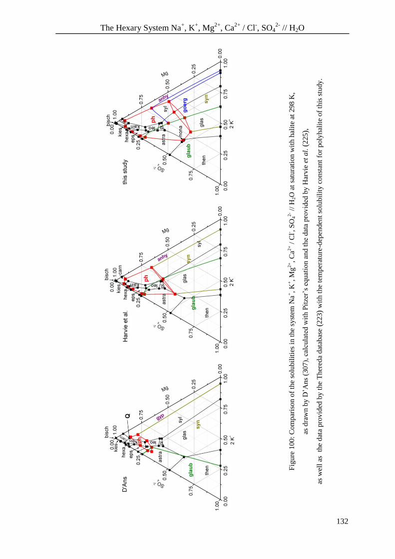
The Hexary System Na+, K
+, Mg
2+, Ca
2+ / Cl
-, SO4
2- // H2O
132
Fig
ure
10
0:
Com
par
iso
n o
f th
e so
lubil
itie
s in
the
syst
em N
a+,
K+, M
g2
+,
Ca2
+ /
Cl- ,
SO
42- /
/ H
2O
at
satu
rati
on
wit
h h
alit
e at
29
8 K
,
as d
raw
n b
y D
’Ans
(307
), c
alcu
late
d w
ith P
itze
r’s
equat
ion a
nd t
he
dat
a pro
vid
ed b
y H
arvie
et
al.
(2
25),
as w
ell
as
the
dat
a pro
vid
ed b
y t
he
Ther
eda
dat
abas
e (2
23)
wit
h t
he
tem
per
ature
-dep
enden
t so
lub
ilit
y c
on
stan
t fo
r p
oly
hal
ite
of
this
stu
dy
.
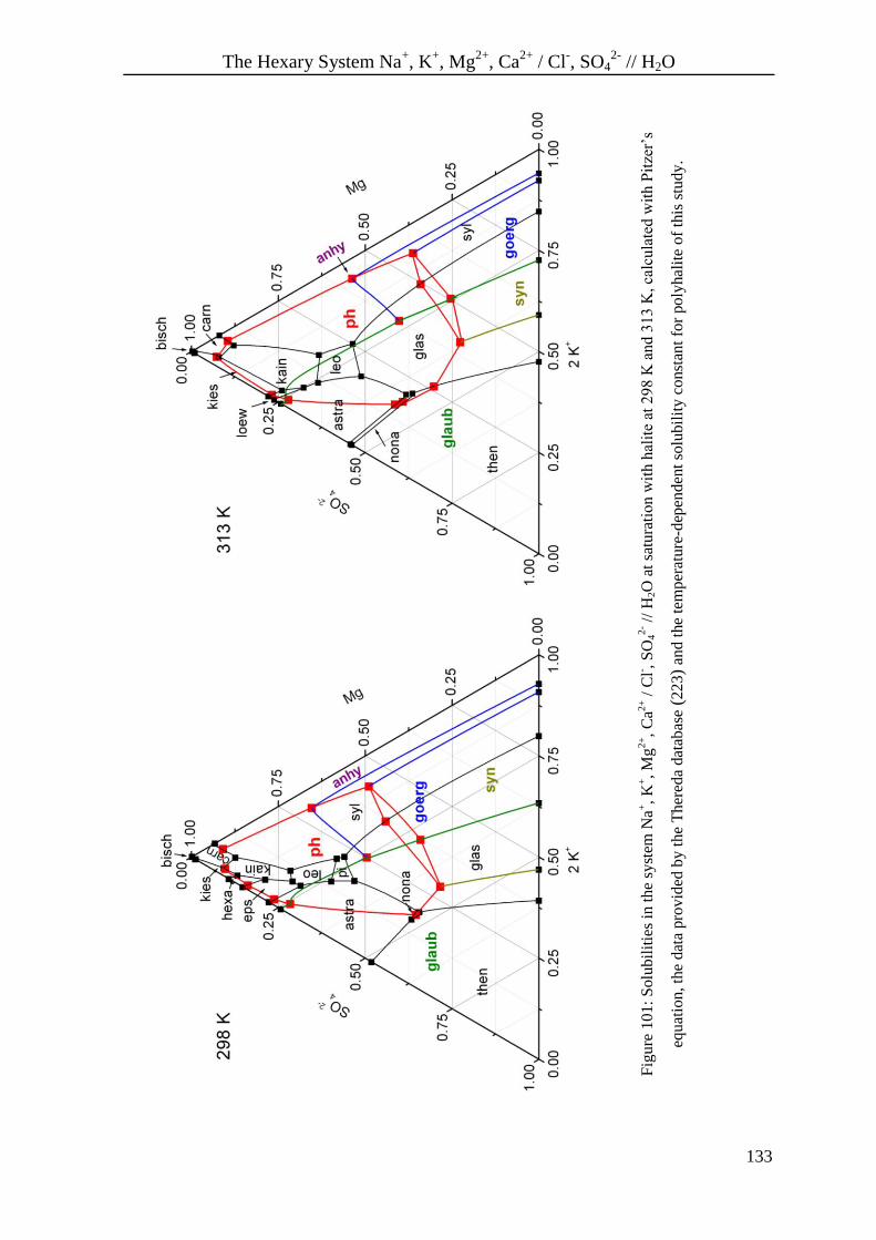
The Hexary System Na+, K
+, Mg
2+, Ca
2+ / Cl
-, SO4
2- // H2O
133
Fig
ure
10
1:
Solu
bil
itie
s in
th
e sy
stem
Na
+,
K+, M
g2
+,
Ca2
+ /
Cl- ,
SO
42
- //
H2O
at
satu
rati
on w
ith h
alit
e at
29
8 K
an
d 3
13
K, ca
lcu
late
d w
ith P
itze
r’s
equ
atio
n, th
e d
ata
pro
vid
ed b
y t
he
Ther
eda
dat
abas
e (2
23)
and t
he
tem
per
ature
-dep
enden
t so
lubil
ity
co
nst
ant
for
po
lyhal
ite
of
this
stu
dy
.
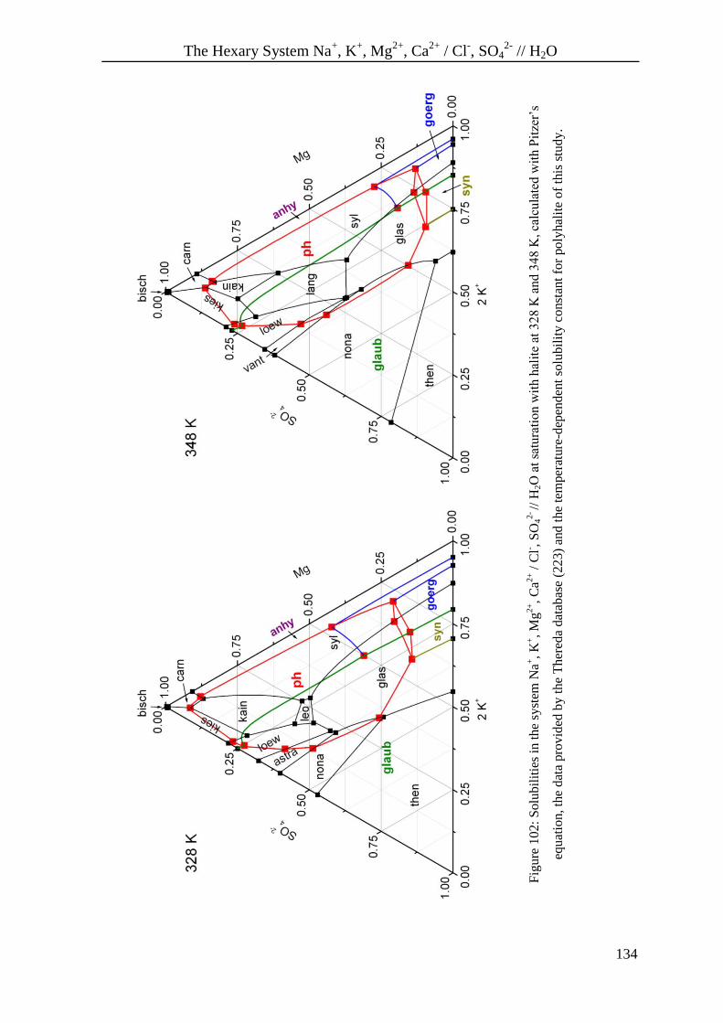
The Hexary System Na+, K
+, Mg
2+, Ca
2+ / Cl
-, SO4
2- // H2O
134
Fig
ure
10
2:
Solu
bil
itie
s in
th
e sy
stem
Na
+,
K+, M
g2
+,
Ca2
+ /
Cl- ,
SO
42
- //
H2O
at
satu
rati
on w
ith h
alit
e at
32
8 K
an
d 3
48
K, ca
lcu
late
d w
ith P
itze
r’s
equ
atio
n, th
e d
ata
pro
vid
ed b
y t
he
Ther
eda
dat
abas
e (2
23
) an
d t
he
tem
per
ature
-dep
enden
t so
lubil
ity
co
nst
ant
for
po
lyhal
ite
of
this
stu
dy
.
Preparation of Substances and Analyses
135
9. Preparation of Substances and Analyses
9.1. Preparation of Substances
All salts employed in the study (see Appendix A – Experimental and Constants) were
analyzed by powder X-ray diffraction. The hydrates were analyzed additionally by thermal
analysis.
Calcium sulfate hemihydrate was obtained by dehydration of gypsum at 373 K for 48 h.
Anhydrite was made by dehydration of gypsum at 243 K for 72 h. Afterwards both solids
were analyzed using Raman spectroscopy and DTA/TG.
Manganese sulfate monohydrate was prepared by dissolving MnSO4·4H2O in deionized
water (Seralpur Pro 90 CN) at 313 K. The supersaturated solution was stirred for three
days. The crystals were filtered from the solution and air dried.
The preparation of polyhalite and its analogues, where Mg2+
is substituted by Mn2+
, Co2+
,
Ni2+
, Cu2+
and Zn2+
, was carried out as follows.
In 150 mL of deionized water, potassium sulfate and the appropriate metal sulfate were
dissolved at the boiling point. After 1.5 hours the solid remaining was filtered off over a
pre-heated fritted disk. Again, the solution was heated to boiling and 10 mL of CaCl2
solution (1.8 mol/L) was added. In the case of leightonite the preparation was completed in
slightly acidic (nitric) solution. The compositions of the initial solutions are given in
Appendix A – Experimental and Constants. The reaction required about 6 hours. Products
were separated on a pre-heated fritted disk and washed with 15 mL each of 85 % and 96 %
ethanol.
All samples were analyzed for phase constituents by Raman spectroscopy and thermal
analysis. For typical impurities as gypsum Raman spectra are more sensitive than powder
X-ray diffraction patterns.
9.2. Analyses of Solutions
The gravimetrical analyses were performed at least twice for each sample and the titrations
at least three times. The average of the determinations gives the result.
Preparation of Substances and Analyses
136
9.2.1. Sodium Analyses
The amount of sodium in the NaClO4 solutions was measured using a Carl-Zeiss-Jena
AAS 3 atomic absorption spectrometer at a wavelength of 330.3 nm. Solutions were
prepared with Cs-La-Buffer (Schinkel) and determined with calibration. The measurements
were carried out in an air-acetylene flame with flow rates of 400 L/min (air) and 60 L/min
(acetylene). The error of the resulting molality of the NaClO4 solutions was within
± 0.5 %.
9.2.2. Potassium Analyses
The analyses of potassium were performed by precipitation of potassium
tetraphenylborate. The bivalent metal ions (Mg2+
, Ca2+
, Mn2+
, Co2+
, Ni2+
, Cu2+
, Zn2+
)
contained in solution, were complexed with EDTA and a pH of 9 was established in
solution. Then sodium tetraphenylborate was added, the solid filtered off and dried at
378 K.
9.2.3. Magnesium Analyses
Magnesium in solution was analyzed by direct titration of magnesium with EDTA using
Erio T as indicator. In solution a pH of 10 was set and the solution titrated with EDTA
until the color changed from red to blue.
9.2.4. Calcium Analyses
Calcium was determined by ICP-OES with an Optima 3000 instrument (Perkin Elmer),
using the emission line at 396.847 nm. The analysis was performed by the standard
addition method with inductively-coupled plasma optical emission spectrometry (ICP-
OES) to deal with every sample separately. This assures the lowest influence of non-
spectroscopic interferences, especially because the densities of the samples are very
different due to the high concentration differences of the MSO4 present (M = Mg, Mn, Co,
Ni, Cu, Zn). This leads to noticeable differences in viscosity even for relatively dilute
solutions. With increasing metal sulfate concentration, the solutions have to be diluted
more and more. Therefore, the amount of calcium for analysis in the diluted solutions
decreases with increasing metal sulfate concentration, which is amplified by the decrease
of gypsum solubility at high metal sulfate concentrations.
The measurements required dilution ratios in the range of 1:100 to 1:1000. For each data
point a blank, the sample, and two addition steps were measured. These four solutions
Preparation of Substances and Analyses
137
were prepared by weighing. For the samples separated from the ternary systems
Ca2+
, M2+
/ SO42-
// H2O (M = Mg, Mn, Co, Ni, Cu, Zn), the blank consisted of an MSO4
(M = Mg, Mn, Co, Ni, Cu, Zn) stock solution diluted to the appropriate concentration as in
the diluted sample. Blanks for the samples extracted from the quaternary systems
K+, Ca
2+, M
2+/ SO4
2- // H2O (M = Mg, Mn, Co, Ni, Cu, Zn) were made by dilution of
K2SO4 and MSO4 (M = Mg, Mn, Co, Ni, Cu, Zn) stock solutions. For the addition steps,
the same weight of sample was used as for the pure diluted sample. Addition of an
appropriate amount of calcium sulfate from a stock solution requires a rough estimate of
the CaSO4 concentration in the sample solution. For these estimations, solubility data of
the 298 K and 323 K isotherm of the Ca2+
, Mn2+
/ SO42-
// H2O system published by Zhelnin
et al. (57) were used for the determination of the solutions separated from the ternary
systems Ca2+
, M2+
/ SO42-
// H2O. The approximation of the calcium concentration in the
quaternary systems K+, Ca
2+, M
2+/ SO4
2- // H2O was performed using information about the
amount of calcium sulfate hemihydrate that could be added before a solid appeared in
solution.
In the first addition step, the same amount of calcium sulfate as assumed in the sample was
added. In the second addition step, twice as much was added. The sample, the first addition
step, and the second addition step were diluted in the same amount of water, taking into
account the water added by the calcium sulfate addition.
ICP-OES measurements were carried out at an RF power of 1300 W with a nebulizer gas
flow of 0.8 L/min, an auxiliary gas flow of 0.5 L/min, and a coolant gas flow of 15 L/min.
The molality of calcium in the sample was calculated by linear regression of the measured
intensities versus added calcium molality. For this, the intensity of the blank was
subtracted from the sample and the two addition steps. The linear regression was
completed with uncertainty estimated at 95 % probability.
9.2.5. Manganese Analyses
For the analysis of Mn2+
the solution was first acidified with hydroxylamine and then
heated to boiling. For neutralizing, sodium hydroxide solution was added and afterward,
magnesium complexonate solution, as well as ammonia and Erio T. The titration was
conducted with EDTA to the blue end-point.
Preparation of Substances and Analyses
138
9.2.6. Cobalt Analyses
Cobalt was measured by complexometric titration. Murexide was added to the slightly
acidic solution. To the violet solution just as much ammonia was added until a yellow
coloring persisted. The titration was carried out with EDTA to the purple end-point.
9.2.7. Nickel Analyses
Nickel was analyzed gravimetrically as bis(dimethylglyoximato)nickel(II). To the acidic
sample solution dimethylglyoxime solution was added drop wise. The resulting solid was
filtered off and dried at 383 K.
9.2.8. Copper Analyses
Copper in solution was determined with EDTA and Murexide. A slightly acidic solution
was combined with Murexide and ammonia added until a yellow color persisted. The
titration was completed with EDTA to the purple end-point.
9.2.9. Zinc Analyses
Complexometric titration of zinc was executed by buffering the solution at pH 10 and
titrating with EDTA using Erio T as indicator to the blue end-point.
9.3. Characterization of the Solids
9.3.1. Powder X-ray Diffraction
The analyses were conducted using a D5000 (Siemens) system using Cu K radiation in
the 10-50° 2 range and a collection time of 1 s / 0.02° step. The recorded patterns were
matched against the PDF2-file of the International Centre for Diffraction Data and an
internal database.
9.3.2. Raman Spectroscopic Analyses
Raman spectra were recorded with a Bruker RFS 100/S FT-spectrophotometer. The
samples were placed in aluminum holders and measured from 1200 cm-1
to 350 cm-1
with a
1064 nm laser (75 mW) with 200 accumulation cycles.
Preparation of Substances and Analyses
139
9.3.3. Thermal Analyses
Thermal analysis was performed with a Seiko DTA/TG 22 apparatus using 10 mg to 20 mg
of sample in a platinum crucible at a heating rate of 5 K/min up to 773 K under nitrogen
flow.

Conclusion
140
10. Conclusion
Phase equilibrium studies of the hexary oceanic salt system Na+, K
+, Mg
2+, Ca
2+ / Cl
-,
SO42-
// H2O are fundamental for assessment studies of chemotoxic waste disposals in rock
salt formations. There, the abundantly distributed mineral polyhalite
K2SO4·MgSO4·2CaSO4·2H2O is considered to respond as a natural heavy metal sink,
because the Mg2+
ion can be substituted by other bivalent metal ions. In this work, the
heavy metal ions substituted in polyhalite were limited to Mn2+
, Co2+
, Ni2+
, Cu2+
, Zn2+
.
Determinations of mineral solubilities in multi-electrolyte solutions require extensive
experimental work. Modelling the systems allows the prediction of these properties for
complex mixtures based on information obtained from simple systems. One of these
quantities needed is the solubility constant Ksol. In order to determine the solubility
constants of the heavy metal-containing polyhalites, knowledge about the molalities,
activity coefficients, and water activity is needed. The basic system, where polyhalite
occurs, is K+, Mg
2+, Ca
2+ / SO4
2- // H2O. Therefore the solubility determinations of
polyhalite and its substituted analogues were performed in the quaternary systems
K+, M
2+, Ca
2+ / SO4
2- // H2O (M = Mg, Mn, Co, Ni, Cu, Zn). Since polyhalite forms slowly
over months or years at 298 K, the solid-liquid phase equilibria experiments were
accomplished at 313 K.
The determination of the activity coefficients and the water activity requires extensive
studies especially for mixed electrolyte solutions at high ionic strengths. For this reason,
Pitzer’s equations were used. Working with this model, knowledge of binary ion
interactions MX+
- SO42-
(M = K, Ca, Mg, Mn, Co, Ni, Cu, Zn) and mixing ion interactions
NX+
, M2+
- SO42-
(N = K, Ca; M = Ca, Mg, Mn, Co, Ni, Cu, Zn) is necessary at 298 K as
well as at 313 K. For modelling the stability field of polyhalite and its analogues, the
solubility constants of the surrounding solid phases are required also. For this reason, not
only the quaternary systems but also the ternary and binary systems are relevant.
Because the solid-liquid phase equilibrium studies of the quaternary systems have to be
performed at 313 K, the enthalpies of dissolution are needed to extrapolate lnKsol from
313 K to 298 K.
This work has made one of its main focuses the systematic evaluation of published data.
The evaluation of the solubility data showed considerable deficiencies in the ternary
systems. For the systems Ca2+
, M2+
/ SO42-
// H2O, almost no solubility data has been
published at any temperature. Most of the systems K+, M
2+ / SO4
2- // H2O are described
Conclusion
141
well at 298 K, but deficiencies at higher temperatures are revealed. Solubility
investigations of the heavy metal-containing polyhalites in the corresponding quaternary
systems are completely lacking.
In order to improve this data situation, solubility determinations have been performed for
the system K+, Mg
2+ / SO4
2- // H2O at 318 K,
the system K+, Mn
2+ / SO4
2- // H2O at 298 K and 313 K,
the system K+, M
2+ / SO4
2- // H2O (M = Co, Ni, Cu, Zn) at 313 K,
the system Ca2+
, M2+
/ SO42-
// H2O (M = Mg, Mn, Co, Ni, Cu, Zn) at 298 K and
313 K,
the system K+, Ca
2+, M
2+ / SO4
2- // H2O (M = Mg, Mn, Co, Ni, Cu, Zn) at 313 K.
Because the solid-liquid phase equilibria investigations of the quaternary systems had to be
executed at 313 K, Pitzer parameters at this temperature as well as at 298 K were
necessary.
For the heavy metal sulfates, binary parameters are available only at 298 K, the same is
encountered for the mixing parameters for K+-M
2+-SO4
2-. In the case of CoSO4, even the
parameters of 298 K needed a reinvestigation. So far, interactions for Ca2+
-M2+
-SO42-
(Mg, Zn) have only been published at 298 K. For the other heavy metals, parameters have
not been determined at any temperature.
Hence, the estimation of the Pitzer parameters has been accomplished for
the binary interactions for M2+
-SO42+
(M = Mn, Co, Ni, Cu, Zn) from 298 K to
323 K,
the mixing interactions for K+-M
2+-SO4
2+ (M = Mn, Co, Ni, Cu, Zn) at 313 K and
for K+-Mn
2+-SO4
2+ also at 298 K, as well as the determination of the solubility
constants of the associated double salts,
the mixing interactions for Ca2+
-M2+
-SO42+
(M = Mn, Co, Ni, Cu, Zn) at 298 K and
313 K.
Analyses of calcium in concentrated bivalent metal sulfate solutions are known to be
difficult. Therefore, calcium was determined by ICP-OES with the standard-addition
method, dealing with every sample separately. This assured the lowest influence of non-
spectroscopic interferences, especially since the densities of the samples are very different,
due to the high concentration differences of MSO4. Furthermore, the calcium concentration
decreases noticeably at high concentrations of MSO4.
Solubility studies of the ternary systems K+-M
2+-SO4
2+ and Ca
2+-M
2+-SO4
2+ (M = Mg, Mn,
Co, Ni, Cu, Zn) were performed by the isothermal saturation method.
Conclusion
142
In the system K+-Mg
2+-SO4
2+ at 318 K, epsomite, leonite, picromerite and arcanite appear
as solid phases along the obtained isotherm. This is the first time that a complete solubility
isotherm with simultaneous crystallization branches of leonite and picromerite has been
investigated. For attaining phase equilibrium, the experiments lasted up to 100 days.
The ternary system K+, Mn
2+ / SO4
2- // H2O was determined at 298 K and 313 K. At 298 K,
the solid phases MnSO4·H2O, K2SO4·3MnSO4·5H2O, K2SO4·MnSO4·4H2O and K2SO4
appear with increasing potassium sulfate concentrations. Hence, the formation of
K2SO4·3MnSO4·5H2O was proven at 298 K. Examination of the system at 313 K revealed
that K2SO4·MnSO4·1.5H2O was formed besides MnSO4·H2O, K2SO4·2MnSO4 and K2SO4.
The double salt K2SO4·MnSO4·2H2O was also found at this temperature, forming a
metastable equilibrium in the system. The investigations showed for the first time a
stability field for K2SO4·MnSO4·1.5H2O. From this study it can be concluded that the
system K+, Mn
2+ / SO4
2- // H2O needs to be reinvestigated with extended equilibration
times below 273 K and above 313 K.
Solubility equilibria in the systems K+, M
2+ / SO4
2- // H2O (M = Co, Ni, Cu, Zn) were
determined at 313 K. In the four systems involving potassium sulfate, the corresponding
heavy metal sulfate hydrate (CoSO4·7H2O, -NiSO4·6H2O, CuSO4·5H2O, ZnSO4·6H2O)
and the double salt K2SO4·MSO4·6H2O was formed. The Tutton’s salt shows in all systems
an extended crystallization branch. In the system K+, Ni
2+ / SO4
2- // H2O the crystallization
branch of the double salt dominates and causes the stability field of K2SO4 to almost
disappeare.
In the literature, only few data are provided for the ternary systems
Ca2+
, M2+
/ SO42-
// H2O (M = Mg, Mn, Co, Ni, Cu, Zn). Gypsum solubility in MSO4-H2O
media (M = Mg, Mn, Co, Ni, Cu, Zn) was determined at 298 K and 313 K. In magnesium
sulfate solutions, the solubility of anhydrite was examined at 333 K as well. The new data
allow for the first time a systematic comparison of the influence of a series of bivalent
metal sulfates on the solubility of gypsum. The general trend of solubility variation on
MSO4 concentration is the same for all investigated systems and at all temperatures
studied. In solutions of MgSO4, gypsum solubility is significant lower than in all other
MSO4 solutions. The solubility of gypsum in solutions of MSO4 (M = Mn, Co, Cu, Zn) is
the same within the experimental error. For NiSO4 solutions at molalities
5.14NiSOm molal the solubility decreases more steeply and the data approach the curve
for the system with MgSO4.
Conclusion
143
The quaternary systems K+, Ca
2+, M
2+ / SO4
2- // H2O (M = Mg, Mn, Co, Ni, Cu, Zn) were
investigated at 313 K. Over the examined concentration range, polyhalite crystallized in all
systems except for M = Ni. The absence of polyhalite in the nickel-containing system is
caused by the low solubility of K2SO4·NiSO4·6H2O. The fields of the polyhalites are
surrounded by the corresponding bivalent metal sulfate hydrates and the Tutton’s salt at
high bivalent metal sulfate concentrations. In the case of the system
K+, Ca
2+, Mn
2+ / SO4
2- // H2O, K2SO4·2MnSO4 appears instead of K2SO4·MnSO4·6H2O.
Investigations of the magnesium-, manganese- and cobalt-containing systems showed that
at small concentrations of potassium sulfate the polyhalite field is restrained by that of
metastable gypsum. Limitation of the polyhalite field at low concentrations of bivalent
metal sulfate was not established experimentally within the examined concentration range.
The curves for the two-salt equilibria of the polyhalites with the metal sulfate hydrates and
the Tutton’s salts, as well as of K2SO4·2MnSO4, do not vary noticeably from the solubility
isotherm in the ternary systems K+, M
2+ / SO4
2- // H2O at 313 K. The same pattern is
encountered for the solubility curve of gypsum and polyhalite in comparison to the systems
Ca2+
, M2+
/ SO42-
// H2O.
In determining the solubility constants for the polyhalites from the solubility data of the
quaternary systems, the activity coefficients of the solute components had to be derived. In
this work the Pitzer model was employed for this task. Therefore, the binary and mixing
parameters were required at 313 K, as well as at 298 K, to calculate the stability fields at
298 K.
The binary parameters for MSO4 were estimated in the temperature range from 283 K to
323 K, basing them on parameters published at 298 K. In the case of CoSO4, the
parameters at 298 K had to be re-evaluated. From the ternary systems
K+, M
2+ / SO4
2- // H2O and Ca
2+, M
2+ / SO4
2- // H2O, the Pitzer mixing parameters were
derived at 298 K and 313 K. For Ca2+
, Mg2+
/ SO42-
// H2O, additional parameters were
estimated at 333 K. Furthermore, the solubility constants for the solids forming in the
binary and ternary systems at 298 K and 313 K have been estimated.
The enthalpy of dissolution gives a basis to extrapolate the solubility constant of polyhalite
from 313 K to 298 K. For this reason, the enthalpy of dissolution of polyhalite and its
analogues has been determined in NaClO4 solutions of varying ionic strengths from
0.5 molal NaClO4 to 2.0 molal NaClO4 at 298 K. All polyhalites dissolve exothermally.
With increasing NaClO4 concentrations the integral heat of dissolution becomes more
exothermic.

Conclusion
144
Extrapolation to infinite dilution was performed using the SIT model. The enthalpy of
dissolution of K2MgCa2(SO4)4·2H2O with M = Mg, Mn, Ni, Zn coincides within
experimental uncertainties, except for M = Cu, leightonite.
With the determined solid-liquid equilibrium data for the systems K+, M
2+, Ca
2+ / SO4
2- //
H2O (M = Mg, Mn, Co, Ni, Cu, Zn) and the estimated parameters, solubility constants
were calculated at 313 K, and extrapolated with msolH to 298 K.
The solubility constants for the polyhalites were applied to calculate the solubility
equilibria in the quaternary systems K+, M
2+, Ca
2+ / SO4
2- // H2O (M = Mg, Mn, Co, Cu,
Zn) at 298 K and 313 K. For all systems it was found that with increasing temperature the
stability field of the polyhalites grows, especially at the expense of syngenite. Leightonite
has the largest stability field and therefore the lowest solubility constant.
Including solubility data of the literature, the solubility constant of Mg-polyhalite was re-
evaluated for the temperature range from 298 K to 373 K. The solubility data are well
represented by the model and the determined solubility constant. At 298 K, a larger
crystallization field resulted for Mg-polyhalite than has been published, although some
reasonable doubts about the published solubility data can be raised.
With Pitzer parameters from the literature and the estimated solubility constants, the
crystallization fields in the hexary system Na+, K
+, Mg
2+, Ca
2+ / Cl
-, SO4
2- // H2O were
calculated at NaCl saturation. Here, it was found also that with increasing temperature, the
polyhalite field is larger than previously thought.
A comparison of the crystallization fields in the hexary system saturated with sodium
chloride at 298 K shows an increase of the polyhalite field from D’Ans (307) to Harvie et
al. (225) and this study. In view of this work and the extensive compilation of literature
data, the dimension of the stability field of polyhalite as considered so far at 298 K has to
be questioned. New reliable solubility experiments for the system K+, Mg
2+, Ca
2+ / SO4
2- //
H2O are inevitable required at 298 K, although they are extremely time consuming or have
to be performed with a technique that remains to be developed.
Bibliography
145
11. Bibliography
1 van't Hoff, J. H.: Z. anorg. Chem. 47 (1905) 244
2 D'Ans, J.: Kali 9 (1915) 193
3 Voigt, W.; Brendler, V.; Marsh, K.; Rarey, R.; Wanner, H.; Gaune-Escard, M.;
Cloke, P.; Vercouter, T.; Bastrakov, E.; Hagemann, S.:
Pure Appl. Chem. 79 (2007) 883
4 Altmaier, M.; Brendler, V.; Hagemann, S.; Herbert, H.-J.; Kienzler, B.; Marquardt,
C. M.; Moog, H. C.; Neck, V.; Richter, A.; Voigt, W.; Wilhelm, S.:
atw 53 (2008) 249
5 Clarke, L.; Partridge, E. P.: Ind. Eng. Chem. 26 (1934) 897
6 Autenrieth, H.: Kali Steinsalz 2 (1958) 181
7 Chipera, St. J.; Vaniman, D. T.: Geochim. Cosmochim. Acta 71 (2007) 241
8 Peterson, R. C.; Wang, R.: Geology 34 (2006) 957
9 Nobst, P.; Ludwig, H.-M.; Stark, J.: Wiss. Z. Hochsch. Archit. Bauwes. Weimar 40
(1994) 119
10 Band 7: Bauchemie; Erster Workshop Bauchemie; GDCh-Arbeitsgemeinschaft
Bauchemie; 25. - 26. November 1996 in Hünfeld bei Fulda; hrsg. von H. Behret,
1997
11 Luckas, M.; Krissmann, J., thermodynamic der Elektrolytlösungen, Springer
Verlag, Berlin, 2001
12 Pitzer, K. S., Activity Coefficients in Electrolyte Solutions, second ed., CRC press
Inc., Boca Raton, 1991
13 Grenthe, I.; Puigdomenech, I. (Eds.), Modelling in Aquatic Chemistry, OECD
Publications, Paris, 1997, pp. 325-426
14 Archer, D. G.; Wang, P.: J. Phys. Chem. Ref. Data. 19 (1990) 371
15 Benrath, A.; Benrath, H.: Z. anorg. Chem. 184 (1929) 359
16 Lepeshkov, I. N.; Novikova L. V.: Zh. Neorg. Khim. 3 (1958) 2395
17 Bodaleva, N. V.; Lepeshkov, I. N.: Zh. Neorg. Khim. 1 (1956) 995
18 Lukyanova, E. I.; Sokol, V. I.; Sokolova, G. N.: Zh. Neorg. Khim. 1 (1956) 298
19 Ricci, J. E.; Fischer, J.: J. am. Chem. Soc. 74 (1952) 1443
20 Hill, A. E.: J. Am. Chem. Soc. 56 (1934) 1071
21 Benrath, A.: Z. anorg. Chem. 189 (1930) 82
22 Weston, A.: J. chem. Soc. 121 (1922) 1223

Bibliography
146
23 Caven, R. M.; Johnston, W.: J. chem. Soc. (1926) 2628
24 Caven, R. M.; Mitchell, T. C.: J. chem. Soc. 125 (1924) 1428
25 Caven, R. M.; Johnston, W.: J. chem. Soc. (1927) 2358
26 Campbell, A. N.; Downes, K. W.; Samis, C. S.: J. Am. Chem. Soc. 56 (1934) 2507
27 Benrath, A.; Benrath, H.: Z. anorg. Chem. 189 (1930) 72
28 Bayliss, N. S.; Cole, A. R. H.; Ewers, W. E.; Jones, N. K.:
J. am. Chem. Soc. 69 (1947) 2033
29 van der Heide, J. K.: Z. phys. Chem. 2 (1893) 416
30 Benrath, A.; Sichelschmidt, A.: Z. anorg. Chem. 197 (1931) 113
31 Perova, A. P.: Zh. Neorg. Khim. 15 (1970) 2821
32 Legrand, M.; Paris, R. E.: Bull. Soc. Chim. France 8 (1966) 2699
33 Caven, R. M.; Johnston, W.: J. chem. Soc. 131 (1928) 2506
34 Shevchuk, V. G.; Lazorenko, N. M.; Dryuchko, A. G.; Skorikov, V. M.:
Zh. Neorg. Khim. 24 (1979) 3390
35 Filippov, V. K.; Rumyantsev, A. V.: Zh. Prikl. Khim. 61 (1988) 2622
36 Shevchuk, V. G.; Pilipchenko, V. N..: Zh. Neorg. Khim. 11 (1966) 432
37 Usmanova, M. Kh.; Druzhinin, I. G.:
Ucenye Zapiski Mosk. Obl. Pedagog. Inst. 236 (1969) 101
38 D'Ans, J.; Kaufmann, E.: Z. anorg. u. allgem. Chem. 290 (1957) 334
39 Nathans, M. W.: J. Phys. Chem. 67 (1963) 1248
40 Legrand, M.; Paris, R. A.: Bull. Soc. Chim. France 11 (1967) 4283
41 Filippov, V. K.; Yakovleva, S. I.: Zh. Prikl. Khim. 52 (1979) 564
42 Shevchuk, V. G.; Pavlenko, A. I.: Zh. Prikl. Khim. 44 (1971) 183
43 Hidalgo, A. Veintemillas, S.; Rodriguez-Celemente, R.; Molins, E.; Balarev, Chr.;
Keremidchieva, B.; Spasov, V.: Z. Kristallogr. 211 (1996) 153
44 Druzhinin, I. G.; Usmanova, N. Kh.:
Ucenye Zapiski Mosk. Obl. Pedagog. Inst. 236 (1969) 107
45 Filippov, V. K.; Antonova, V. A.; Foland, P.; Chaiko, I. G.: Vestn. Leningr. Univ.,
Fiz. Khim. 22 (1982) 63
46 Nadzhafova, T. A.; Abdullaeva, T. N.; Alieva, U. R.; Gasymova, Sh. A.:
Azerb. Khim. Zh. 2 (1988) 102
47 Flöttmann, Fr.: Z. anal. Chem. 73 (1928) 1
48 Gmelin Handbuch der Anorganischen Chemie, 8. Auflage, Kalium, Teil A, Verlag
Chemie GmbH, Weinheim, 1942
Bibliography
147
49 Karnaukhov, A. S.; Runov, N. N.: Izv. Vyssh. Uchebn. Zaved., Khim. Khim.
Tekhnol. 12 (1967) 1299
50 Zhelnin B. I., Gorshtein G. I.: Zh. Neorg. Khim. 20 (1975) 20
51 Korf D. M., Fomina E. A.: Zh. Neorg. Khim. 8 (1963) 1022
52 Hill A.E.: J. am. Chem. Soc. 59 (1937) 2242
53 D'Ans J., Bredtschneider D., Eick H.: Kali Steinsalz 9 (1955) 17
54 Valuziene B. A., Vesiene T. B., Lashkova L. N.: Zh. Neorg. Khim. 13 (1968) 1198
55 Hill A. E., Yanick N. S.: J. Am. Chem. Soc. 57 (1935) 645
56 Novikova L. V.: Zh. Neorg. Khim. 2 (1957) 662
57 Zhelnin B. I., Gorshtein G. I., Bezprozvannaya L. Kh.:
Zh. Prikl. Khim. 46 (1973) 506
58 Campbell A. N., Yanick N. S.: Trans. Faraday soc. 28 (1932) 657
59 Karnaukhov, A. S.; Fedorenko, T. P.; Vaisfel'd, M. I.; Onishchenko, M. K.;
Shevchuk, V. G.: Zh. Neorg. Khim. 19 (1974) 1981
60 Bytyrchaev, I. E.; Ryspaev, O.: Izv. Akad. Nauk Kirg.SSR4 (1972) 59
61 Lepeshkov, I. N.; Fradkina, Kh. B.: Zh. Neorg. Khim. 4 (1959) 2803
62 Harkins, W. D.; Paine, H. M.: J. Am. Chem. Soc. 41 (1919) 1155
63 Tanji, K. K.: Environ. Sci. Technol. 3 (1969) 656
64 D'Ans, J.: Kali Steinsalz 5 (1968) 109
65 Posnjak, E.: Am. J. Sci. 35A (1938) 247
66 Partridge, E. P.; White, A. H.: J. Am. Chem. Soc. 51 (1929) 360
67 Hulett, G. A.; Allen, L. E.: J. Am. Chem. Soc. 24 (1902) 667
68 Hulett, G. A.: Z. phys. Chem. 37 (1901) 385
69 Hall, R. E.; Robb, J. A.; Coleman, C. E.: J. Am. Chem. Soc. 48 (1926) 927
70 Denman, W. L.: J. Ind. Eng. Chem. 53 (1961) 817
71 Bock, E.: Can. J. Chem. 39 (1961) 1746
72 Sborgi, U.; Bianchi, C.: Gazz. Chim. Ital. 70 (1940) 823
73 Melcher, A. C.: J. Am. Chem. Soc. 32 (1910) 50
74 Marshall, W. L.; Slusher, R.: J.Chem. Thermodynamics 5 (1973) 189
75 Kalyanaraman, R.; Yeatts, L. B.; Marshall, W. L.:
J. Chem. Thermodynamics 5 (1973) 891
76 Booth, H. S.; Bidwell, R. M.: J. Am. Chem. Soc. 72 (1950) 2567
77 Power, W. H.; Fabuss, B. M.; Satterfield, C. N.: J. Chem. Eng. Data 9 (1964) 437
78 Chassevent, L.: Ann. Chim. Appl. 6 (1926) 244

Bibliography
148
79 Chassevent, L.: Ann. Chim. Appl. 6 (1926) 313
80 Block, J.; Waters, O. B., Jr.: J. Chem. Eng. Data 13 (1968) 336
81 Mutalala, B. K.; Umetsu, Y.; Tozawa, K.: Tohoku Daigaku Senko Seiren
Kenkyusho Iho 44 (1988) 57
82 Farrah, H. E.; Lawrance, G. A.; Wanless, E. J.: Hydrometallurgy 86 (2007) 13
83 Genceli, F. E.; Lutz, M.; Spek, A. L.; Witkamp, G.: Crystal Growth & Design 7
(2007) 2460
84 D'Ans J.: Ber. Dtsch. Chem. Ges. 41 (1908) 187
85 Autenrieth H.: Kali Steinsalz (1954) 3
86 Averina, R. A.; Shevchuk, V. G.: Zh. Neorg. Khim. 14 (1969) 1321
87 Filippov, V. K.; Cheremnykh, L. M.: Vestn. Leningr. Univ., Fiz. Khim. 3 (1983) 32
88 Filippov, V. K.; Nokhrin, V. I.: Zh. Neorg. Khim. 30 (1985) 501
89 Oikova, T.; Balarev, Chr.; Makarov, L. L.: Z. phys. Chem. 156 (1975) 890
90 Averina, R. A.; Shevchuk, V. G: Zh. Neorg. Khim. 12 (1967) 3138
91 Tembotov, B. K.; Druzhinin, I. G.: Sb. Nauch. Rab. Aspir. Kabardino-Balkar.
Univ. 2 (1968) 333
92 Litvinov, S. D.; Danilov, V. P.; Lepeshkov, I. N.: Zh. Neorg. Khim. 28 (1983) 3201
93 Danilov, V. P.; Lepeshkov, I. N.; Litvinov, S. D.; Krasnobaeva, O. N.:
Zh. Neorg. Khim. 25 (1980) 1432
94 Lepeshkov, I. N.; Romashova, N. N.: Zh. Neorg. Khim. 5 (1960) 2512
95 Lepeshkov, I. N.; Romashova, N. N.: Zh. Neorg. Khim. 4 (1959) 2812
96 Benrath, V. A.; Neumann, E.: Z. anorg. allgem. Chem. 242 (1939) 70
97 Benrath, A.: Z. anorg. allg. Chem. 247 (1941) 147
98 Benrath, A.; Blankenstein, A.: Z. anorg. allg. Chem. 216 (1933) 41
99 Hildebrand, J. H.: J. Ind. Eng. Chem. 10 (1918) 96
100 Schroeder, W.: Z. anorg. allg. Chem 184 (1929) 63
101 Benrath, A.; Pitzler, H.; Ilieff, N.; Beu, W.; Schloemer, A.; Clermont, J.;
Kojitsch, S.; Benrath, H.: Z. anorg. allg. Chem. 170 (1928) 257
102 Robson, H. L.: J. Am. Chem. Soc. 49 (1927) 2772
103 Zhelnin, B. I.; Gorshtein, G. I.: Zh. Neorg. Khim. 16 (1971) 3146
104 Balarev, Chr.; Tepavitcharova, S.; Rabadjieva, D.; Voigt, W.: J.
Solution Chem. 30 (2001) 815
105 Pillay, V.; Gaertner, R. S.; Himawan, C.; Seckler, M. M.; Lewis, A. E.;
Witkamp, G.-J.: J. Chem. Eng. Data 50 (2005) 551

Bibliography
149
106 Oikova, T.; Barkov, D.: Zh. Neorg. Khim. 24 (1979) 501
107 Filippov, V. K.; Nokhrin, V. I.: Zh. Neorg. Khim. 30 (1985) 501
108 Shevchuk, V. G.; Kost, L. L.: Zh. Neorg. Khim. 12 (1967) 1069
109 Ting, H. H.; McCabe, W. L.: J. Ind. Eng. Chem. 11 (1934) 1207
110 Kuchkarov, Kh.; Tukhtaev, S.: Uzb. Khim. Zh. (1983) 3
111 Oikova, T.; Balarev, Chr.; Makarov, L. L.: Zh. Fiz. Khim. 50 (1976) 347
112 Gmelin Handbuch der Anorganischen Chemie, 8. Auflage, Magnesium, Teil B,
Verlag Chemie GmbH, Weinheim, 1939
113 Schreinemakers, F. A. H.: Chem. Weekblad 6 (1909) 131
114 Filippov, V. K.; Nokhrin, V. I.; Krylova, I. L.: Vestn. Leningr. Univ.,
Fiz. Khim. 3 (1985) 45
115 Shevchuk, V. G.; Storozhenko, V. A.; Petrov, G. V.:
Zh. Neorg. Khim. 38 (1993) 546
116 Benrath, A.: Z. anorg. allg. Chem. 183 (1929) 296
117 Benrath, A.; Benrath, H.: Z. anorg. allg. Chem. 179 (1929) 369
118 Druzhinin, I. G.; Gorokhova, V. N.: Izv. Akad. Nauk Kirg. SSR, Ser. Estestv. i
Tekhn. Nauk 4 (1962) 81
119 Benrath, A.; Blankenstein, A.: Z. anorg. allg. Chem.217 (1934) 170
120 Filippov, V. K.; Charykov, N. A.: Zh. Neorg. Khim. 34 (1989) 1613
121 Petlicka, J.: Hutn. Listy. 10 (1970) 727
122 Soroka, P. I.; Girich, T. E.; Simich, M. L.: Zh. Neorg. Khim. 33 (1988) 1058
123 Soroka, P. I.; Girich, T. E.; Simich, M. L.: Zh. Neorg. Khim. 31 (1986) 1608
124 Maksimenko, A. A.; Shevchuk, V. G.: Zh. Prikl. Khim. 47 (1974) 541
125 Shevchuk, V. G.; Maksimenko, A. A.: Zh. Prikl. Khim. 45 (1972) 2338
126 Dzyuban, N. K.; Kovalenko, T. A.: Zh. Neorg. Khim. 30 (1985) 2443
127 Maksimenko, A. A.; Shevchuk, V. G.: Zh. Neorg. Khim. 18 (1973) 1401
128 Rohmer, R.: C.R. Hebd. Seances Acad. Sci. 209 (1939) 315
129 Cottrell, F. G.: J. Phys. Chem 4 (1900) 637
130 Dzhabarov, A. I.; Agaev, A. I.; Aliev, V. A.: Uch. Zap., Azerb. Univ.,
Ser. Khim. Nauk 2 (1971) 3
131 Krepelka, J. H.; Rejha, B.: Collect. Czech. Chem. Commun. 5 (1933) 67
132 Baichalova, S.; Imanakunov, B.: Izv. Akad. Nauk Kirg.SSR 6 (1970) 48
133 Nguyen Q. N.; Reshetnikova, L. P.; Novoselova, A. V.: Vestn. Mosk. Univ.,
Ser. 2. Khim. 13 (1972) 483

Bibliography
150
134 Druzhinin, I. G.; Duishenalieva, N.: Izv. Akad. Nauk Kirg. SSR, Ser. Estestv. i
Tekhn. Nauk 2 (1960) 85
135 Druzhinin, I. G.; Duishenalieva, N.; Ismanova, B.:
Izv. Akad. Nauk Kirg. SSR (1974) 38
136 Druzhinin, I. G.; Gorokhova, V. N.: Izv. Vyssh. Uchebn. Zaved.,
Khim. Khim. Tekhnol. (1961) 765
137 Oikova, T.; Makarov, L. L.: Zh. Fiz. Khim. 50 (1976) 2130
138 Dzhabarov, A. I.; Agaev, A. I.; Aliev, V. A.: Uch. Zap. Azerb. Univ. Ser. Khim.
Nauk (1970) 6
139 Gmelin Handbuch der Anorganische Chemie, 8. Auflage, Mangan, Teil C 6,
Springer Verlag, Berlin 1976
140 Caven R. M., Gardner W. K.: J. chem. Soc. (1933) 943
141 Filippov, V. K.; Yakovleva, S. I.; Dmitriev, G. V.: Vestn. Leningr. Univ.,
Fiz. Khim. 3 (1979) 58
142 Filippov, V. K.; Charykov, N. A.; Solechnik, N. D.:
Zh. Prikl. Khim. 58 (1986) 1966
143 Bassett, H.; Henshall, J. H.: J. chem. Soc. (1950) 1970
144 Filippov, V. K.; Yakovleva, S. I.: Zh. Neorg. Khim. 24 (1979) 2793
145 Benrath, A.; Thiemann, W.: Z. anorg. allg. Chem. 217 (1934) 347
146 Crockford, H. D.; Brawley, D. J.: J. Phys. Chem 36 (1932) 1594
147 Zavitskaya, V. I.: Zh. Neorg. Khim. 15 (1970) 2835
148 Zavitskaya, V. I.: Zh. Neorg. Khim. 19 (1974) 1110
149 Kondrateva, N. G.; Beskov, S. D.: Zh. Neorg. Khim. 15 (1970) 1090
150 Shevchuk, V. G.; Pavlenko, A. I.: Zh. Neorg. Khim. 15 (1970) 2522
151 Druzhinin, I. G.; Kondrat'eva, N. G.: Zh. Neorg. Khim. 11 (1966) 2803
152 Bursa, S.; Stanisz-Lewicka, M.: Zh. Neorg. Khim. 25 (1980) 2534
153 Bakaev, A. M.; Margulis, E. V.: Zh. Neorg. Khim. 23 (1978) 243
154 Koppel, J.: Z. phys. Chem. 52 (1905) 385
155 Langauer, D.: Z. anorg. allg. Chem. 213 (1933) 180
156 Bruhn, G.; Gerlach, J.; Pawlek, F.: Z. anorg. allg. Chem. 337 (1965) 68
157 Ganz, S. N.; Karchevskii, A. V.; Braginskaya, R. I.; Repka, G. I.:
Zh. Prikl. Khim. 47 (1974) 1494
158 Shevchuk, V. G.; Pavlenko, A. I.: Zh. Prikl. Khim. 44 (1971) 183
159 Blidin, V. P.; Andreeva, T. A.: Zh. Neorg. Khim. 3 (1958) 2414
Bibliography
151
160 Rohmer, R.: C.R. Hebd. Seances Acad. Sci. 199 (1934) 641
161 Shevchuk, V. G.; Storozhenko, D. A.; Kisel, N. N.:
Zh. Neorg. Khim. 25 (1980) 838
162 Storozhenko, D. A.; Shevchuk, V. G.: Zh. Neorg. Khim. 24 (1979) 2812
163 Suratkar, T. S.; Mehta, S. M.; Prasad: Proc. Indian Natl. Sci. Acad.,
Part A 7 (1938) 393
164 Balarev, Chr.; Oikova, T.: Izv. Khim. 8 (1975) 640
165 Brodale, G. E.; Giauque, W. F.: J. Phys. Chem 69 (1965) 1268
166 Gmelin Handbuch der Anorganischen Chemie, 8. Auflage, Kobalt, Teil A, Verlag
Chemie GmbH, Weinheim, 1961
167 Hill A. E., Taylor W. J.: J. Am. Chem. Soc. 60 (1938) 1099
168 Benrath A.: Z. anorg. Chem. 202 (1931) 161
169 Simich, M. L.; Kharchenko, V. A.; Girich, T. E.; Soroka, P. I.:
Zh. Neorg. Khim. 37 (1992) 2341
170 Filippov, V. K.; Veretennikova, G. A.; Nokhrin, V. I.:
Zh. Prikl. Khim. 57 (1984) 1938
171 Druzhinin, I. G.; Kuznetsov, V. G.; Imanakunov, B.: Izvest. Akad. Nauk Kirgiz.
S.S.R., Ser. Estestven, i Tekh. Nauk 2 (1960) 25
172 Addlestone, J. A.: J. Phys. Chem 42 (1938) 437
173 Kudryashov, Yu. E.; Lebedev, A. E.: Zh. Prikl. Khim. 62 (1989) 700
174 Girich, T. E.; Buchinskii, A. K: Zh. Prikl. Khim. 59 (1986) 884
175 Chretien, A.; Rohmer, R.: C. R. Hebd.Seances Acad. Sci. 198 (1934) 92
176 Onishchenko, M. K.; Shevchuk, V. G.: Zh. Neorg. Khim. 23 (1978) 1375
177 Onishchenko, M. K.; Skorikov, V. M.; Shevchuk, V. G.:
Zh. Neorg. Khim. 24 (1979) 1099
178 Onishchenko, M. K.; Shevchuk, V. G.; Skorikov, V. M.:
Zh. Neorg. Khim. 24 (1979) 1367
179 Girich, T. E.; Braginskaya, R. I.; Buchinskii, A. K.; Reznichenko, S. I.: Zh. Neorg.
Khim. 31 (1986) 1575
180 Gmelin Handbuch der Anorganischen Chemie, 8. Auflage, Nickel, Teil B, Verlag
Chemie GmbH, Weinheim, 1966
181 Schreinemakers F. A. H.: Z. phys. Chem. 69 (1910) 557
182 Schreinemakers F. A. H.: Z. phys. Chem. 66 (1909) 687
183 Massink A.: Z. phys. Chem. 92 (1917) 351
Bibliography
152
184 Foote, H. W.: J. Ind. Eng. Chem. 11 (1919) 629
185 Akbaev, A.; Ezhova, V. V.; Mamatkanov, A.: Zh. Neorg. Khim. 16 (1971) 3172
186 Druzhinin, I. G.; Kosyakina, O. A.: Zh. Neorg. Khim. 6 (1961) 1729
187 Akbaev, A.: Izv. Akad. Nauk Kirg.SSR 5 (1970) 43
188 Filippov, V. K.; Udovenko, A. G.; Nikitin, V. A.; Charykova, M. V.;
Puchkov, L. V.: Zh. Neorg. Khim. 43 (1998) 2095
189 Laptev, V. M.; Akhmarov, F. I.; Dmitrevskii, B. A.; Kamalov, O. K.:
Zh. Prikl. Khim. 65 (1992) 2363
190 Bakeev, M. I.; Shkodina, T. B.; Zharmenov, A. A.; Kalinskaya, N. N.:
Zh. Neorg. Khim. 37 (1992) 1914
191 Bakaev, A. M.; Margulis, E. V.: Zh. Neorg. Khim. 20 (1975) 1117
192 Agde, G.; Barkholt, H.: Angewandte Chemie 39 (1926) 851
193 Occleshaw, V. J.: J. Am. Chem. Soc. 127 (1925) 2598
194 Miles, F. T.; Menzies, A. W. C.: J. Am. Chem. Soc. 59 (1937) 2392
195 Crockford, H. D.; Webster, M. M.: J. Phys. Chem 34 (1930) 2375
196 Karchevskii, A. V.; Mel'nikov, B. I.; Aleshkevich, S. A.; Tkachik, M. I.:
Zh. Prikl. Khim. 62 (1989) 1892
197 Druzhinin, I. G.; Shepelev, A. I.; Gamayunova, A. A.:
Zh. Neorg. Khim. 20 (1975) 2583
198 Cohen, E.; Chattaway, T. D.; Tombrok, W.: Z. physik. Chem. 60 (1908) 706
199 Ganz, S. N.; Karchevskii, A. V.; Braginskaya, R. I.; Selezneva, E. P.:
Izv. Vyssh. Uchebn. Zaved., Khim. Khim. Tekhnol. 16 (1973) 663
200 Babayan, G. G.; Mkhitaryan, R. S.; Panosyan, G. S.; Shakhnazaryan, A. A.:
Arm. Khim. Zh. 26 (1973) 283
201 Novoselova, A. V.; Bodaleva, N. V.; Gershtein, M. M.:
Zh. Obshch. Khim. 8 (1938) 732
202 Gmelin Handbuch der Anorganischen Chemie, 8. Auflage, Kupfer, Teil B, Verlag
Chemie GmbH, Weinheim, 1958
203 Shevchuk V. G., Lepeshkov I. N.: Zh. Neorg. Khim. 1 (1956) 1888
204 Bouchacourt M., Saugier M. T., Cohen-Adad R.: Bull. Soc.
Chim. France 9-10 (1977) 842
205 Nabiev, M. N.; Kucharov, Kh.; Tukhtaev, S.; Borukhov, I. A.:
Zh. Neorg. Khim. 23 (1978) 1691

Bibliography
153
206 Filippov, V. K.; Nokhrin, V. I.; Muzalevskaya, A. P.:
Zh. Neorg. Khim. 30 (1985) 2407
207 Girich, T. E.; Soroka, P. I.; Simich, M. L.: Vopr. Khim.
Khim. Tekhnol. 84 (1987) 17
208 Bury, C. R.: J. Am. Chem. Soc. 125 (1924) 2538
209 Schroeder, W.: Z. anorg. allg. Chem. 228 (1936) 129
210 Duishenalieva, N.; Sulaimankulov, K.; Druzhinin, I. G.:
Zh. Neorg. Khim. 6 (1961) 1919
211 Cohen, E.; Hetterschij, C. W. G.: Z. physik. Chem. 115 (1925) 440
212 Cohen, E.: Z. physik. Chem. 34 (1900) 178
213 Rohmer, R.: C.R. Hebd. Seances Acad. Sci. 210 (1940) 669
214 Shevchuk, V. G.; Moshinskii, A. S.: Zh. Neorg. Khim. 14 (1969) 2507
215 Geroleva, O. V.; Molodkin, A. K.; Druzhinin, I. G.:
Zh. Neorg. Khim. 19 (1974) 1431
216 Pieniazek, T.; Milewska, A.; Masztalerz, P.: Chem. Stosow. 26 (1982) 419
217 Bursa, S.; Stanisz-Lewicka, M.: Chem. Stosow. 25 (1981) 251
218 Balarev, Chr.; Oikova, T.: God. Vissh. Khim.-Tekhnol. Inst. 11 (1976) 309
219 Callendar, H. L.; Barnes H. T.: Proc. R. Soc. Lond. 62 (1897) 117
220 Shevchuk, V. G.; Druzhinin, I. G.: Izv. Vyssh. Uchebn. Zaved.,
Khim. Khim. Tekhnol. (1958) 25
221 Rudolph, W. W.; Brooker, M. H.; Tremaine, P. R.:
J. Solution Chem. 28 (1999) 621
222 Jones, E. V.; Lietzke, M. H.; Marshall, W. L.: J. Am. Chem. Soc. 79 (1957) 267
223 www.Thereda.de; database without Mg-polyhalite and the temperature-dependent
parameters of the Mg-Ca-SO4 ion interaction
224 Harvie, C. E.; Weare, J. H.: Geochim. Cosmochim. Acta 44 (1980) 981
225 Harvie, C. E.; Moeller, N.; Weare, J. H.:
Geochim. et Cosmochim. Acta 48 (1984) 723
226 Greenberg, J. P.; Moller N.: Geochim. Cosmochim. Acta 53 (1989) 2503
227 Christov, C.; Moller, N.: Geochim. Cosmochim. Acta 68 (2004) 1309
228 Christov, C.; Moller, N.: Geochim. Cosmochim. Acta 68 (2004) 3717
229 Petrenko, S. V.; Valyashko, V. M.; Ziegenbalg, G.:
Zh. Neorg. Khim. 37 (1992) 2111
230 Pitzer, K. S.; Mayorga, G.: J. Solution Chem. 3 (1974) 539

Bibliography
154
231 Rard, J. A.: J. Chem. Eng. Data 29 (1984) 443
232 Kim, H. T.; Frederick, W. J., Jr.: J. Chem. Eng. Data 33 (1988) 177
233 El Guendouzi, M.; Mounir, A.; Dinane, A.:
J. Chem. Thermodynamics 35 (2003) 209
234 Robinson, R. A.; Jones, R. S.: J. Am. Chem. Soc. 58 (1936) 959
235 Yokoyama, H.; Yamatera, H.: Bull. Chem. Soc. Japan 48 (1975) 2708
236 Libus, W.; Sadowska, T.; Libus, Z.: J. Solution Chem. 9 (1980) 341
237 Robinson, R. A.; Harned, H. S.: Chem. Rev. 28 (1941) 419
238 Robinson, R. A.; Stokes, R. H.: Trans. Faraday Soc. 45 (1949) 612
239 Pitzer, K. S.: J. Chem. Soc., Faraday Trans. 68 (1972) 101
240 Wagman D. D.; Evans W. H.; Parker V. B.; Schumm R. H.; Halow I.; Bailey S. M.;
Churney K. L.; Nuttall R. L.: J. Phys. Chem. Ref. Data 11,
Supplement No. 2 (1982)
241 Zordan, T. A.; Hepler, L. G.: Chem. Rev. 68 (1968) 737
242 Filippov, V. K.; Dmitriev, G. V.; Yakovleva, S. I.: Doklady Akademii Nauk SSSR
252 (1980) 156
243 Filippov, V. K.; Nokhrin, V. I.: Zh. Neorg. Khim. 30 (1985) 513
244 Christov, C.: J. Chem. Thermodynamics 37 (2005) 1036
245 Christov, C.: J. Chem. Thermodynamics 31 (1999) 71
246 Downes, C. J.; Pitzer, K. S.: J. Solution Chem. 5 (1976) 389
247 Miller, D. G.; Rard, J. A.; Eppstein, L. B.; Robinson, R. A.:
J. Solution Chem. 9 (1980) 467
248 Downes, C. J.; Pitzer, K. S.: J. Solution Chem. 5 (1976) 389
249 Gedansky, L. M.; Woolley, E. M.; Hepler, L. G.:
J. Chem. Thermodynamics 2 (1970) 561
250 Mönig, J.; Herbert H.-J.: „Exemplarische Untersuchungen
vonWechselwirkungsreaktionen UTD-relevanter chemisch-toxischer Abfälle mit
hochsalinaren Lösungen“, GRS-Bericht 126, Braunschweig (1996)
251 Oikova, T.; Makarov, L. L.; Balarev, Chr.; Miloshova, M. S.:
Z. phys. Chem. 255 (1974) 453
252 Miladinovic, J.; Ninkovic, R.; Todorovic, M.; Jovanovic, V.:
J. Solution Chem. 32 (2003) 371
253 Kangro, W.; Groeneveld, A.: Z. phys. Chem. 32 (1962) 110

Bibliography
155
254 Albright, J. G.; Rard, J. A.; Serna, S.; Summers, E. E.; Yang, M. C.:
J. Chem. Thermodynamics 32 (2000) 1447
255 Miladinovic, J.; Todorovic, M.; Ninkovic, R.:
J. Chem. Thermodynamics 34 (2002) 1769
256 Wetmore, F. E. W.; Gordon, A. R.: J. Chem. Phys. 5 (1937) 60
257 Dhillon, D. S.; Blokhra, R. L.: Indian J. Chem. 5 (1967) 340
258 Cowperthwaite, I. A.; La Mer, V. K.: J. Am. Chem. Soc. 53 (1931) 4333
259 Kielland, J.: J. Am. Chem. Soc. 58 (1936) 1855
260 Königsberger, E.; Eriksson, G.: Calphad 19 (1995) 207
261 Schreiber, D. R.; DeWyse, K.; Schreiber, L. C.; Tung, T.:
J. Solution Chem. 28 (1999) 567
262 Silvester, L. F.; Pitzer, K. S.: J. Solution Chem. 7 (1978) 327
263 Riederer K.: PhD thesis “Die Bestimmung thermodynamischer Eigenschaften
verdünnter Elektrolytlösungen aus Messungen der Verdünnungswärme”,
Universität Regensburg, (1981)
264 Soloveva, S. G.; Vlasenko, K. K.; Karapetyants, M. Kh.:
Zh. Fiz. Khim. 51 (1977) 2991
265 Goldberg, R. N.; Riddell, R. G.; Wingard, M. R.; Hopkins, H. P.; Wulff, C. A.;
Hepler, L. G.: J. Phys. Chem 70 (1966) 706
266 Söhnel, O.; Novotny, P.: Densities of aqueous solutions of inorganic substances
(Academia, Prague 1985)
267 Lange, E.; Monheim, J.; Robinson, A. L.: J. Am. Chem. Soc. 55 (1933) 4733
268 Giauque, W. F.; Barieau, R. E.; Kunzler, J. E.: J. Am. Chem. Soc. 72 (1950) 5685
269 Harned, H. S.: J. Am. Chem. Soc. 59 (1937) 360
270 Anderson, E.; Nestell R. J.: J. Ind. Eng. Chem. 12 (1920) 243
271 Cameron, F. K.; Breazeale, J. F.: J. Phys. Chem. 8 (1904) 335
272 Sveshnikova, V. N.: Izv. Akad. Nauk SSSR, Ser. Khim. (1952) 44
273 Litvinenko, V. I.; Erzhanova, R. S.; Bekturov, A. B.: Izv. Akad. Nauk Kaz. SSR,
Ser. Khim. 18 (1968) 1
274 Kurnakov, N. S.; Shoikhet, D. N.: Ann. secteur anal. phys.-chim.,
Inst. chim. gen. (U. S. S. R.) 10 (1938) 305
275 Bozza, G.: Giornale di Chimica Industriale ed Applicata 16 (1934) 106
276 Van Klooster, H. S.: J. Phys. Chem. 21 (1917) 513
277 Levi, S. M.: Z. phys. Chem. 106 (1923) 93

Bibliography
156
278 Perova, A. P.: Zh. Neorg. Khim. 15 (1970) 1927
279 Vyas, S. N.; Venkataraman, R.: Indian J. Technol. 12 (1974) 199
280 Andronova, N. P.; Lepeshkov, I. N.: Zh. Neorg. Khim. 3 (1958) 2156
281 Maeda, K.; Kuramochi, H.; Shinkawa, T.; Fukui, K.:
J. Chem. Eng. Data 47 (2002) 1472
282 Jänecke, E.: Dölters Handbuch der Mineralchemie, Bd. IV, part 2, Verlag von
Theodor Steinkopff, Dresden, 1929
283 Starrs, B. A.; Clarke, L.: J. Phys. Chem. 34 (1930) 1058
284 Starrs, B. A.; Storch, H. H.: J. Phys. Chem. 34 (1930) 2367
285 Usdowski, E.; Dietzel, M.: Atlas and Data of solid-solution equilibria of marine
evaporites, Springer-Verlag, Berlin, 1998
286 Dzhabarov, A. I.; Agaev, A. I.; Aliev, V. A.: Uch. Zap. Azerb.
Univ. Ser. Khim. Nauk (1970) 3
287 Verdiev, D. A.; Aliev, V. A.; Alosmanov, M. S.: Azerb. Khim. Zh. (1984) 104
288 Borene, J.; Solery, J. P.: Acta. Cryst. B28 (1972) 2687
289 Benrath, A.; Ritter, G.: J. prakt. Chem. 154 (1939) 40
290 Benrath, A.: Z. anorg. Chem. 208 (1932) 169
291 Kucharov, Kh.; Tukhtaev, S.; Osichkina, R. G.; Borukhov, I. A.:
Zh. Neorg. Khim. 22 (1977) 2282
292 Tukhtaev, S.; Kucharov, Kh.; Aminov, Z.: Zh. Neorg. Khim. 29 (1984) 2939
293 Borbieva, D.; Imanakunov, B.; Druzhinin, I. G.:
Izv. Akad. Nauk Kirg. SSR 3 (1969) 64
294 Basikhina, L. A.; Druzhinin, I. G.: Zh. Neorg. Khim. 19 (1974) 277
295 Lipscomb, G. F.; Hulett, G. A.: J. Phys. Chem. 20 (1916) 75
296 Bremer, M.; Christov, C.; Voigt, W.: Abschlußbericht zum Vorhaben 02 C 0405,
„Erstellung einer Datenbasis zur Modellierung der Wechselwirkung von chrom-,
kupfer- und nickelhaltigem Deponiegut mit Lösungen des Salzgesteins einer UTD“,
Freiberg (1999)
297 Umetsu, Y.; Mutalala, B. K., Tozawa K.: Tohoku Daigaku Senko Seiren
Kenkyusho Iho 45 (1989) 13
298 Cameron, F. K.; Bell, J. M.: J. Phys. Chem. 10 (1906) 202
299 Arslan, A.; Dutt, G. R.: Soil Sci. 155 (1993) 37
300 Kolosov, A. S.: Trud. Khim.-Metallug. Inst., Sap.-Sibirsk. Filial.
Akad. Nauk. SSSR 35 (1958) 35

Bibliography
157
301 Mutalala, B. K.; Umetsu, Y.; Tozawa, K.: Mat. Trans., JIM 30 (1989) 394
302 Hagemann, S.: “Entwicklung eines thermodynamischen Modells für Zink, Blei und
Cadmium insalinaren Lösungen”, GRS-Bericht 219; Braunschweig (2008) [in
press]
303 Basch, E. E.: PhD Thesis “Die künstliche Darstellung und die Bildungs-
Verhältnisse des Polyhalit“, Friedrich-Wilhelm-Universität zu Berlin (1901)
304 Perova A. P.: Zh. Neorg. Khim. 15 (1970) 1648
305 Conley, J. E.; Gabriel, A.; Partridge, E. P.: J. phys. Chem. 42 (1938) 587
306 Dankiewicz J., Pawlowska-Kozinska D.: Z. anorg. allg. Chem. 488 (1982) 223
307 D’Ans, J: “Die Löslichkeitsgleichgewichte der Systeme der Salze ozeanischer
Salzablagerungen“, Verlagsgesellschaft für Ackerbau m.b.H., Berlin, 1933
308 Risacher, F.; Fritz, B.: Sciences Geologiques, Bulletin 37 (1984) 229
309 Henneberg, E.; Voigt, W.: Abschlußbericht „Vergleich von geochemischen
Rechenprogrammen und Erweiterung der thermodynamischen Datenbasis für die
Modellierung von hochsalinaren Lösungen-Phase I“, TU Bergakademie Freiberg
(1993)
310 Richardson, L. T.; Wells, R. C.: J. Wash. Acad. Sci. 21 (1931) 243
311 Günther, C.; Pfestorf, R.; Rother, M.; Seidel, J.; Zimmermann, R.; Wolf, G.: J.
Thermal Anal. 33 (1988) 359
312 Marsh, K. N. (Eds.), IUPAC, Recommended Reference Materials for the
Realization of Physicochemical Properties, Blackwell Scientific Publications,
Oxford, 1987
313 Beyer, R.: PhD thesis “Charakterisierung von binären und ternären
Elektrolytsystemen mit Anionen organischer Säuren“, Hamburg, 2001
314 Larson, J. W.; Cerutti, P.; Garber, H. K.; Hepler, L. G.:
J. Phys. Chem. 72 (1968) 2902
315 Schmelzer, N.; Grigo, M.; Zorn, B.; Einfeldt, J.: Wissenschaftliche Zeitschrift der
Universität Rostock, Naturwissenschaftliche Reihe 34 (1985) 25
316 Wachter, R.; Riederer, K.: Pure Appl. Chem. 53 (1981) 1301
317 Akilan, C.; Hefter, G.; Rohman, N.; Buchner, R.: J. Phys. Chem. 110 (2006) 14961
318 Capewell, S. G.; Hefter, G. T.; May, P. M.: Talanta 49 (1999) 25
319 Yokoyama, H.; Ohta, T.: Bull. Chem. Soc. Jpn. 62 (1989) 345
320 Reardon, E. J.: J. Phys. Chem. 79 (1975) 422

Bibliography
158
321 Luts, P.; Vanhees, J. L. C.; Yperman, J. J. E.; Mullens, J. M. A.; Van Poucke, L. C.:
J. Sol. Chem. 21 (1992) 375
322 Wollmann, G.; Freyer, D.; Voigt, W.: Monatsh. Chem. 139 (2008) 739
323 Fedoroff, B.; Demassieux, N.: Ann. Chim. Appl. 16 (1941) 154
324 Malatesta, F.; Carbonaro, L.; Fanelli, N.; Ferrini, S.; Giacomelli, A.:
J. Solution Chem. 28 (1999) 593
325 Haring, M. M.; Westfall, B. B.: Trans. Electrochem. Soc. 65 (1934) 235
326 matlab version 7, The MathWorks Inc. 1984-2005
327 chemSage extended version 4.23, Gunnar Eriksson
328 An, L.; Yin, H.; Tang, M.; Yao, L.: Kuangwu Yanshi 24 (2004) 108
329 Autenrieth, H.: Kali Steinsalz 2 (1958) 181
330 Autenrieth, H.; Braune, G.: Kali Steinsalz 2 (1959) 395
331 Kropp, E.; Beate, R.; Grosch, Ch.; Kranz, M.; Holldorf, H.:
Freiberg. Forschungsh. A764 (1988) 42

Appendix A – Experimental and Constants
159
Appendix A – Experimental and Constants
Table 28: Salts employed in the study.
Compounds Purity Distributer
NaClO4·H2O p.a. Fluka
NaNO3 p.a. RdH
K2SO4 p.a. Reachim
MgSO4·7H2O p.a. RdH
CaSO4·2H2O p.a. Fluka
MnSO4·4H2O p.a. Merck
CoSO4·7H2O purr. ABCR
NiSO4·6H2O p.a. Merck
CuSO4·5H2O p.a. Fluka
ZnSO4·7H2O p.a. Fluka

Appendix A – Experimental and Constants
160
Table 29: Composition of the solutions before CaCl2 was added.
compound OHV2
/ mL 4MSOn / mol
42SOKn / mol
polyhalite 150 0.24 0.034
Mn-polyhalite 150 0.17 0.042
Fe-polyhalite 150 0.12 0.040
Co-polyhalite 150 0.12 0.040
Ni-polyhalite 150 0.16 0.040
leightonite 150 0.062 0.022
Zn-polyhalite 150 0.12 0.040
Polynomial for the Debye-Hückel Coefficients Used
The equations are only valid within the given temperature range, at 1 bar and the saturation
vapor pressure, respectively.
Valid within 238-473 K
4
6
2
542321
1
222
1TaTaTa
Ta
TaaA
Valid within 238-423 K
8
13
5.2
125.011102987
111
220
1TaTa
Ta
Ta
Ta
TaaAL
Table 30: Parameters for the polynomial of the Debye-Hückel coefficients used.
Parameter A Parameter AL
a1 -0.8176532151 a7 1297752.477
a2 -0.8685275541 a8 234787.229
a3 19250.991343 a9 -27005964084
a4 0.005251284381 a10 610480968.8
a5 -7.149396961·10-6
a11 -52177636.5
a6 9.338558897·10-12
a12 -0.01371691279
a13 5.337301257·10-18
Appendix B – Experimental Results
161
Appendix B – Experimental Results
Analytical error
Only the cations of the experimental solutions were analyzed.
In the systems M2+
, Ca2+
/ SO42-
// H2O (M = Mg, Mn, Co, Ni, Cu, Zn), the concentrations
of MSO4 were analyzed only at the points where two solid phases were present. The
concentrations of the other solutions were calculated from the weighed amounts of metal
sulfate hydrate and the deionized water.
In case of the systems K+, M
2+, Ca
2+ / SO4
2- // H2O (M = Mn, Co, Ni, Cu, Zn), the added
CaSO4·0.5H2O caused in some solutions only a change of the concentration of potassium
sulfate and the heavy metal sulfate within analytical error; these ions were not analyzed in
the solutions concerned after equilibration. Therefore, no error is given for the
concentration of potassium sulfate and the heavy metal sulfate in these solutions, which
were calculated from the weighed amounts of potassium sulfate, metal sulfate hydrate and
deionized water.
Errors for the ions analyzed gravimetrically, potassium and nickel, were calculated from
trial investigations of the methods with known concentrations, and resulted in a deviation
of 1 to 1.5 %. For calcium, the indicated errors represent an uncertainty at the 95 %
probability level for the Ca analysis determined by the standard addition method. The error
for the M2+
ions (M = Mg, Mn, Co, Cu, Zn) is based on the titration error caused by the
drop size (0.03 mL) of the titration solution. Resulting errors are within 0.5 to 1.5 % of
the total amount of metal ion in the experimental solution.
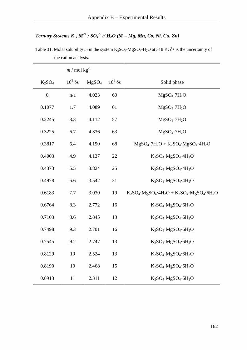
Appendix B – Experimental Results
162
Ternary Systems K+, M
2+ / SO4
2- // H2O (M = Mg, Mn, Co, Ni, Cu, Zn)
Table 31: Molal solubility m in the system K2SO4-MgSO4-H2O at 318 K; δs is the uncertainty of
the cation analysis.
m / mol kg-1
K2SO4 103 δs MgSO4 10
3 δs Solid phase
0 n/a 4.023 60 MgSO4·7H2O
0.1077 1.7 4.089 61 MgSO4·7H2O
0.2245 3.3 4.112 57 MgSO4·7H2O
0.3225 6.7 4.336 63 MgSO4·7H2O
0.3817 6.4 4.190 68 MgSO4·7H2O + K2SO4·MgSO4·4H2O
0.4003 4.9 4.137 22 K2SO4·MgSO4·4H2O
0.4373 5.5 3.824 25 K2SO4·MgSO4·4H2O
0.4978 6.6 3.542 31 K2SO4·MgSO4·4H2O
0.6183 7.7 3.030 19 K2SO4·MgSO4·4H2O + K2SO4·MgSO4·6H2O
0.6764 8.3 2.772 16 K2SO4·MgSO4·6H2O
0.7103 8.6 2.845 13 K2SO4·MgSO4·6H2O
0.7498 9.3 2.701 16 K2SO4·MgSO4·6H2O
0.7545 9.2 2.747 13 K2SO4·MgSO4·6H2O
0.8129 10 2.524 13 K2SO4·MgSO4·6H2O
0.8190 10 2.468 15 K2SO4·MgSO4·6H2O
0.8913 11 2.311 12 K2SO4·MgSO4·6H2O

Appendix B – Experimental Results
163
Table 31 continued
m / mol kg-1
K2SO4 103 δs K2SO4 10
3 δs Solid phase
0.9506 12 2.245 10 K2SO4·MgSO4·6H2O
0.9861 12 1.969 13 K2SO4·MgSO4·6H2O
1.058 13 2.029 10 K2SO4·MgSO4·6H2O + K2SO4
1.028 13 1.489 12 K2SO4
1.003 13 0.999 11 K2SO4
0.9662 11 0.512 8.7 K2SO4
0.9213 11 0 n/a K2SO4
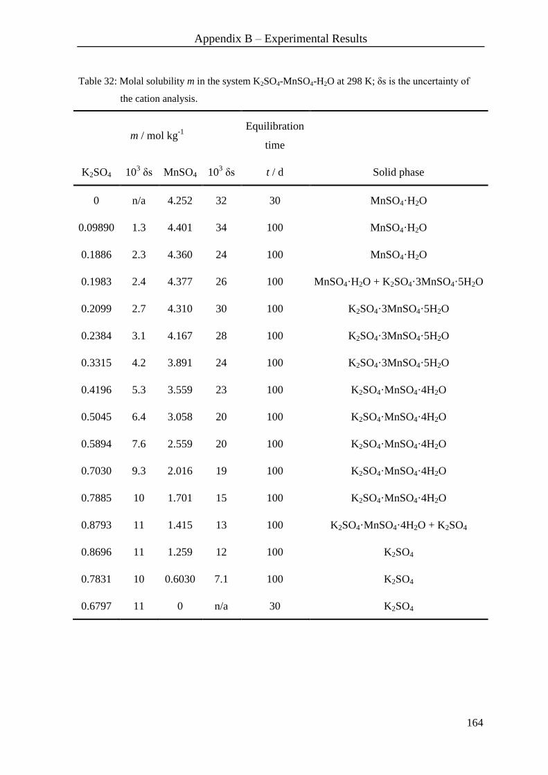
Appendix B – Experimental Results
164
Table 32: Molal solubility m in the system K2SO4-MnSO4-H2O at 298 K; δs is the uncertainty of
the cation analysis.
m / mol kg-1
Equilibration
time
K2SO4 103 δs MnSO4 10
3 δs t / d Solid phase
0 n/a 4.252 32 30 MnSO4·H2O
0.09890 1.3 4.401 34 100 MnSO4·H2O
0.1886 2.3 4.360 24 100 MnSO4·H2O
0.1983 2.4 4.377 26 100 MnSO4·H2O + K2SO4·3MnSO4·5H2O
0.2099 2.7 4.310 30 100 K2SO4·3MnSO4·5H2O
0.2384 3.1 4.167 28 100 K2SO4·3MnSO4·5H2O
0.3315 4.2 3.891 24 100 K2SO4·3MnSO4·5H2O
0.4196 5.3 3.559 23 100 K2SO4·MnSO4·4H2O
0.5045 6.4 3.058 20 100 K2SO4·MnSO4·4H2O
0.5894 7.6 2.559 20 100 K2SO4·MnSO4·4H2O
0.7030 9.3 2.016 19 100 K2SO4·MnSO4·4H2O
0.7885 10 1.701 15 100 K2SO4·MnSO4·4H2O
0.8793 11 1.415 13 100 K2SO4·MnSO4·4H2O + K2SO4
0.8696 11 1.259 12 100 K2SO4
0.7831 10 0.6030 7.1 100 K2SO4
0.6797 11 0 n/a 30 K2SO4

Appendix B – Experimental Results
165
Table 33: Molal solubility m in the system K2SO4-MnSO4-H2O at 313 K; δs is the uncertainty of
the cation analysis.
m / mol kg-1
Equilibration
time
K2SO4 103 δs MnSO4 10
3 δs t / d Solid phase
0 n/a 4.066 36 30 MnSO4·H2O
0.1026 1.4 4.069 36 28 MnSO4·H2O
0.1917 2.4 4.066 24 28 MnSO4·H2O
0.1992 2.5 4.067 24 28 MnSO4·H2O + K2SO4·2MnSO4
0.3061 3.7 3.508 18 28 K2SO4·2MnSO4
0.4020 5.2 3.145 23 66 K2SO4·2MnSO4
0.5259 6.8 2.947 21 28 K2SO4·2MnSO4
0.5721 7.8 2.753 27 66 K2SO4·2MnSO4
0.6070 7.9 2.705 21 66 K2SO4·2MnSO4
0.7057 9.3 2.667 21 95 K2SO4·MnSO4·1.5H2O
0.7542 10 2.478 22 95 K2SO4·MnSO4·1.5H2O
0.8179 11 2.083 15 95 K2SO4·MnSO4·1.5H2O
1.024 13 1.405 11 28 K2SO4·MnSO4·1.5H2O
1.052 13 1.217 8.6 28 K2SO4
0.9532 12 0.6083 4.1 28 K2SO4
0.8810 10 0.2097 1.0 28 K2SO4
0.8618 11 0 n/a 28 K2SO4
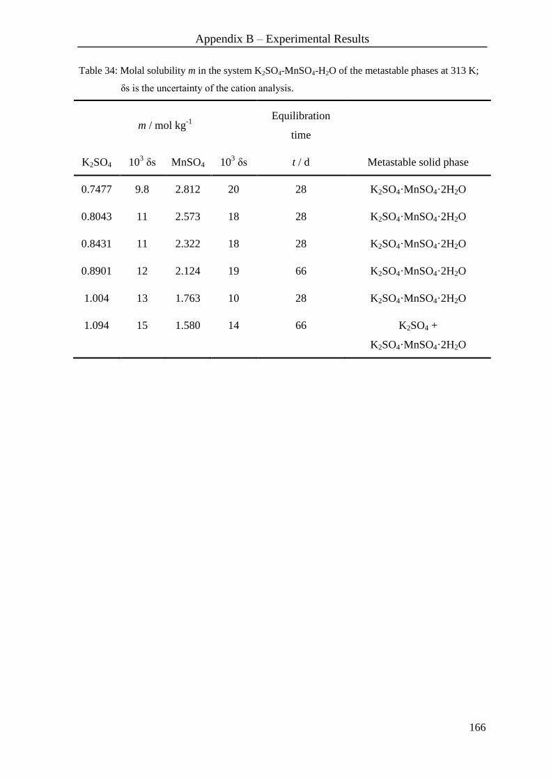
Appendix B – Experimental Results
166
Table 34: Molal solubility m in the system K2SO4-MnSO4-H2O of the metastable phases at 313 K;
δs is the uncertainty of the cation analysis.
m / mol kg-1
Equilibration
time
K2SO4 103 δs MnSO4 10
3 δs t / d Metastable solid phase
0.7477 9.8 2.812 20 28 K2SO4·MnSO4·2H2O
0.8043 11 2.573 18 28 K2SO4·MnSO4·2H2O
0.8431 11 2.322 18 28 K2SO4·MnSO4·2H2O
0.8901 12 2.124 19 66 K2SO4·MnSO4·2H2O
1.004 13 1.763 10 28 K2SO4·MnSO4·2H2O
1.094 15 1.580 14 66 K2SO4 +
K2SO4·MnSO4·2H2O
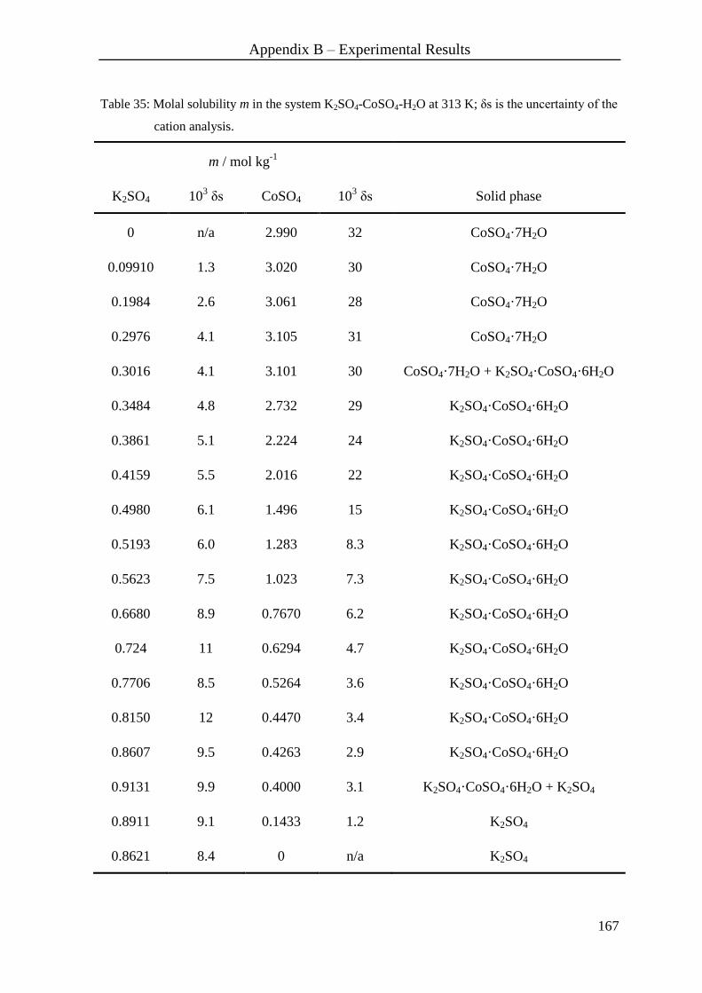
Appendix B – Experimental Results
167
Table 35: Molal solubility m in the system K2SO4-CoSO4-H2O at 313 K; δs is the uncertainty of the
cation analysis.
m / mol kg-1
K2SO4 103 δs CoSO4 10
3 δs Solid phase
0 n/a 2.990 32 CoSO4·7H2O
0.09910 1.3 3.020 30 CoSO4·7H2O
0.1984 2.6 3.061 28 CoSO4·7H2O
0.2976 4.1 3.105 31 CoSO4·7H2O
0.3016 4.1 3.101 30 CoSO4·7H2O + K2SO4·CoSO4·6H2O
0.3484 4.8 2.732 29 K2SO4·CoSO4·6H2O
0.3861 5.1 2.224 24 K2SO4·CoSO4·6H2O
0.4159 5.5 2.016 22 K2SO4·CoSO4·6H2O
0.4980 6.1 1.496 15 K2SO4·CoSO4·6H2O
0.5193 6.0 1.283 8.3 K2SO4·CoSO4·6H2O
0.5623 7.5 1.023 7.3 K2SO4·CoSO4·6H2O
0.6680 8.9 0.7670 6.2 K2SO4·CoSO4·6H2O
0.724 11 0.6294 4.7 K2SO4·CoSO4·6H2O
0.7706 8.5 0.5264 3.6 K2SO4·CoSO4·6H2O
0.8150 12 0.4470 3.4 K2SO4·CoSO4·6H2O
0.8607 9.5 0.4263 2.9 K2SO4·CoSO4·6H2O
0.9131 9.9 0.4000 3.1 K2SO4·CoSO4·6H2O + K2SO4
0.8911 9.1 0.1433 1.2 K2SO4
0.8621 8.4 0 n/a K2SO4
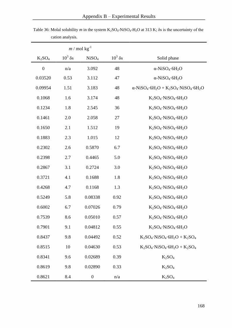
Appendix B – Experimental Results
168
Table 36: Molal solubility m in the system K2SO4-NiSO4-H2O at 313 K; δs is the uncertainty of the
cation analysis.
m / mol kg-1
K2SO4 103 δs NiSO4 10
3 δs Solid phase
0 n/a 3.092 48 α-NiSO4·6H2O
0.03520 0.53 3.112 47 α-NiSO4·6H2O
0.09954 1.51 3.183 48 α-NiSO4·6H2O + K2SO4·NiSO4·6H2O
0.1068 1.6 3.174 48 K2SO4·NiSO4·6H2O
0.1234 1.8 2.545 36 K2SO4·NiSO4·6H2O
0.1461 2.0 2.058 27 K2SO4·NiSO4·6H2O
0.1650 2.1 1.512 19 K2SO4·NiSO4·6H2O
0.1883 2.3 1.015 12 K2SO4·NiSO4·6H2O
0.2302 2.6 0.5870 6.7 K2SO4·NiSO4·6H2O
0.2398 2.7 0.4465 5.0 K2SO4·NiSO4·6H2O
0.2867 3.1 0.2724 3.0 K2SO4·NiSO4·6H2O
0.3721 4.1 0.1688 1.8 K2SO4·NiSO4·6H2O
0.4268 4.7 0.1168 1.3 K2SO4·NiSO4·6H2O
0.5249 5.8 0.08338 0.92 K2SO4·NiSO4·6H2O
0.6002 6.7 0.07026 0.79 K2SO4·NiSO4·6H2O
0.7539 8.6 0.05010 0.57 K2SO4·NiSO4·6H2O
0.7901 9.1 0.04812 0.55 K2SO4·NiSO4·6H2O
0.8437 9.8 0.04492 0.52 K2SO4·NiSO4·6H2O + K2SO4
0.8515 10 0.04630 0.53 K2SO4·NiSO4·6H2O + K2SO4
0.8341 9.6 0.02689 0.39 K2SO4
0.8619 9.8 0.02890 0.33 K2SO4
0.8621 8.4 0 n/a K2SO4

Appendix B – Experimental Results
169
Table 37: Molal solubility m in the system K2SO4-CuSO4-H2O at 313 K; δs is the uncertainty of the
cation analysis.
m / mol kg-1
K2SO4 103 δs CuSO4 10
3 δs Solid phase
0 n/a 1.828 4.6 CuSO4·5H2O
0.09335 0.39 1.851 4.8 CuSO4·5H2O
0.1961 1.42 1.913 4.5 CuSO4·5H2O
0.2059 1.6 1.845 4.3 CuSO4·5H2O
0.2991 2.0 1.982 3.1 CuSO4·5H2O
0.3303 2.8 1.971 3.1 CuSO4·5H2O + K2SO4·CuSO4·6H2O
0.3403 2.4 1.988 3.3 CuSO4·5H2O + K2SO4·CuSO4·6H2O
0.3538 2.3 1.832 1.2 K2SO4·CuSO4·6H2O
0.3739 2.6 1.610 1.2 K2SO4·CuSO4·6H2O
0.4162 2.3 1.270 1.6 K2SO4·CuSO4·6H2O
0.4611 3.1 1.016 1.6 K2SO4·CuSO4·6H2O
0.5390 3.6 0.6647 1.1 K2SO4·CuSO4·6H2O
0.6188 4.4 0.4654 2.0 K2SO4·CuSO4·6H2O
0.7463 5.3 0.3097 1.1 K2SO4·CuSO4·6H2O
0.8077 6.0 0.2726 1.2 K2SO4·CuSO4·6H2O
0.8378 5.9 0.2492 1.3 K2SO4·CuSO4·6H2O
0.8860 10 0.1968 1.9 K2SO4·CuSO4·6H2O + K2SO4
0.8890 10 0.1937 1.9 K2SO4·CuSO4·6H2O + K2SO4
0.8770 10 0.1878 1.4 K2SO4
0.8745 9.8 0.09298 0.93 K2SO4
0.8628 9.4 0.07411 1.7 K2SO4
0.8621 8.4 0 n/a K2SO4

Appendix B – Experimental Results
170
Table 38: Molal solubility m in the system K2SO4-ZnSO4-H2O at 313 K; δs is the uncertainty of the
cation analysis.
m / mol kg-1
K2SO4 103 δs ZnSO4 10
3 δs Solid phase
0 n/a 4.344 19 ZnSO4·6H2O
0.09333 1.1 4.332 19 ZnSO4·6H2O
0.1560 1.8 4.423 17 ZnSO4·6H2O + K2SO4·ZnSO4·6H2O
0.1573 1.9 4.398 19 K2SO4·ZnSO4·6H2O
0.1722 2.3 4.065 34 K2SO4·ZnSO4·6H2O
0.1760 2.1 4.035 18 K2SO4·ZnSO4·6H2O
0.2144 2.6 3.550 16 K2SO4·ZnSO4·6H2O
0.2504 3.0 3.036 14 K2SO4·ZnSO4·6H2O
0.2974 3.6 2.364 15 K2SO4·ZnSO4·6H2O
0.3420 3.9 2.004 8.5 K2SO4·ZnSO4·6H2O
0.3945 4.5 1.511 6.5 K2SO4·ZnSO4·6H2O
0.4398 5.1 1.128 6.1 K2SO4·ZnSO4·6H2O
0.4575 5.1 0.8485 3.6 K2SO4·ZnSO4·6H2O
0.5345 6.1 0.8825 3.4 K2SO4·ZnSO4·6H2O
0.6021 6.9 0.4721 2.8 K2SO4·ZnSO4·6H2O
0.7877 9.1 0.2921 1.5 K2SO4·ZnSO4·6H2O
0.9464 11 0.2388 1.3 K2SO4·ZnSO4·6H2O + K2SO4
0.8997 10 0.1490 0.67 K2SO4
0.8621 8.4 0 n/a K2SO4

Appendix B – Experimental Results
171
Ternary Systems Ca2+
, M2+
/ SO42-
// H2O (M = Mg, Mn, Co, Ni, Cu, Zn)
Table 39: Gypsum, CaSO4·2H2O, solubility as molality in aqueous MgSO4 at 298 K and 313 K; δs
is the 95 % confidence limit.
T = 298 K T = 313 K
m / mol kg-1
m / mol kg-1
MgSO4 CaSO4 104 δs MgSO4 CaSO4 10
4 δs
0 0.0157 3.5 0 0.0158 2.5
0.0108 0.0127 4.8 0.00901 0.0143 5.3
0.0250 0.0115 4.7 0.0258 0.0129 0.0057
0.0495 0.0112 5.5 0.0503 0.0122 7.4
0.102 0.0106 3.1 0.0996 0.0120 6.6
0.201 0.0111 1.5 0.246 0.0129 8.6
0.398 0.0118 7.5 0.501 0.0140 4.5
0.547 0.0125 5.7 0.819 0.0147 7.6
0.685 0.0131 7.2 1.10 0.0147 9.6
0.991 0.0134 10.2 1.40 0.0141 4.7
1.31 0.0135 2.4 1.74 0.0140 9.4
1.83 0.0124 6.2 2.10 0.0126 9.7
2.11 0.0110 3.3 2.50 0.0120 7.7
2.19 0.0112 6.7 2.70 0.0104 7.2
2.48 0.0102 7.4 2.93 0.00842 4.5
2.79 0.00855 6.6 3.21 0.00822 2.5
3.10a
0.00769a
4.2 3.37 0.00764 6.8
3.11b
0 n/a 3.72a
0.00669a
5.6
3.74b
0 n/a
aSolid phases: MgSO4·7H2O and CaSO4·2H2O;
bSolid phase: MgSO4·7H2O.

Appendix B – Experimental Results
172
Table 40: Anhydrite, CaSO4, solubility as molality in aqueous MgSO4 at 333 K; δs is the 95 %
confidence limit.
m / mol kg-1
m / mol kg-1
MgSO4 CaSO4 104 δs MgSO4 CaSO4 10
4 δs
0 0.0115 1.4 2.20 0.01417 1.2
0.0105 0.0114 2.3 2.64 0.01052 6.3
0.0256 0.01131 5.2 3.11 0.00976 4.3
0.0500 0.01058 1.0 3.58 0.00815 3.9
0.0988 0.01054 7.0 4.09 0.00625 3.1
0.2460 0.01123 8.0 4.35 0.00458 3.7
0.5115 0.01315 7.8 4.40 0.00428 1.5
0.921 0.01465 11.2 4.06 0.00671 4.7
1.35 0.01387 6.8 4.48a
0.00426a
3.2
1.76 0.01645 3.0 4.50b
0 n/a
aSolid phases: MgSO4·6H2O and CaSO4;
bSolid phase: MgSO4·6H2O.

Appendix B – Experimental Results
173
Table 41: Gypsum, CaSO4·2H2O, solubility as molality in aqueous MnSO4 at 298 K and 313 K; δs
is the 95 % confidence limit.
T = 298 K T = 313 K
m / mol kg-1
m / mol kg-1
MnSO4 CaSO4 104 δs MnSO4 CaSO4 10
4 δs
0 0.0157 3.5 0 0.0158 2.5
0.0118 0.0135 7.8 0.0281 0.0120 7.9
0.0561 0.0119 1.5 0.0549 0.0110 6.6
0.111 0.0116 0.34 0.115 0.00962 11.1
0.164 0.0121 4.3 0.167 0.0108 9.3
0.280 0.0125 8.2 0.224 0.0122 8.3
0.388 0.0132 4.5 0.448 0.0138 5.5
0.546 0.0139 6.6 0.894 0.0157 10.2
0.891 0.0151 2.6 1.34 0.0165 8.5
1.12 0.0149 6.1 1.79 0.0167 9.3
1.68 0.0146 8.5 2.24 0.0149 8.8
2.18 0.0131 6.8 2.62 0.0135 6.9
2.74 0.0107 4.3 3.11 0.0117 2.1
3.34 0.00804 6.0 3.60 0.0105 0.085
3.86 0.00614 4.7 3.91 0.00888 2.3
4.31a
0.00524a
4.1 4.07a
0.00806a
1.8
4.32a
0.00547a
0.13 4.10a
0.00839a
3.3
4.25b
0 n/a 4.07b
0 n/a
aSolid phases: MnSO4·H2O and CaSO4·2H2O;
bSolid phase: MnSO4·H2O.

Appendix B – Experimental Results
174
Table 42: Gypsum, CaSO4·2H2O, solubility as molality in aqueous CoSO4 at 298 K and 313 K; δs
is the 95 % confidence limit.
T = 298 K T = 313 K
m / mol kg-1
m / mol kg-1
CoSO4 CaSO4 104 δs CoSO4 CaSO4 10
4 δs
0 0.0157 3.5 0 0.0158 2.5
0.0107 0.0130 4.9 0.0105 0.0137 7.2
0.0262 0.0124 6.3 0.0240 0.0133 8.0
0.0507 0.0115 5.6 0.0509 0.0128 5.5
0.100 0.0116 2.1 0.0989 0.0123 3.8
0.251 0.0121 5.1 0.176 0.0129 2.6
0.496 0.0134 8.9 0.251 0.0138 3.2
0.756 0.0147 6.9 0.500 0.0149 8.3
0.986 0.0152 5.1 0.750 0.0166 9.9
1.21 0.0150 2.0 1.00 0.0168 4.5
1.39 0.0152 8.3 1.31 0.0170 15.1
1.61 0.0148 5.4 1.60 0.0176 1.8
1.78 0.0146 8.8 1.89 0.0160 3.7
2.02 0.0139 6.3 2.21 0.0157 10.1
2.25 0.0132 2.9 2.50 0.0145 10.0
2.43 0.0131 7.8 2.80 0.0133 6.9
2.59 0.0126 2.2 2.97 0.0131 2.9
2.81a
0.0118a
7.3 3.08 0.0118 6.9
2.78b
0 n/a 3.28a
0.0116a
8.0
2.99b
0 n/a
aSolid phases: CoSO4·6H2O and CaSO4·2H2O;
bSolid phase: CoSO4·6H2O.

Appendix B – Experimental Results
175
Table 43: Gypsum, CaSO4·2H2O, solubility as molality in aqueous NiSO4 at 298 K and 313 K; δs
is the 95 % confidence limit.
T = 298 K T = 313 K
m / mol kg-1
m / mol kg-1
NiSO4 CaSO4 104 δs NiSO4 CaSO4 10
4 δs
0 0.0157 3.5 0 0.0158 2.5
0.00974 0.0124 5.3 0.0115 0.0134 8.2
0.0252 0.0115 3.1 0.0248 0.0130 10.1
0.0494 0.0115 5.9 0.0534 0.0121 4.8
0.0991 0.0111 7.5 0.0997 0.0127 1.1
0.252 0.0120 4.5 0.251 0.0132 4.6
0.445 0.0132 6.3 0.399 0.0148 4.3
0.587 0.0136 8.9 0.596 0.0157 9.1
0.751 0.0149 5.2 0.877 0.0160 5.6
1.00 0.0151 6.5 1.20 0.0169 11.6
1.26 0.0148 5.7 1.50 0.0168 5.1
1.50 0.0147 7.9 1.81 0.0158 10.1
1.76 0.0138 8.8 2.08 0.0134 4.0
2.02 0.0126 4.1 2.36 0.0131 4.5
2.25 0.0118 7.8 2.70 0.0113 6.2
2.48 0.0103 6.0 3.13c
0.0101c
2.8
2.68a
0.0104a
4.6 3.09d
0 n/a
2.68a
0.0102a
7.9
2.66a
0.0103a
3.7
2.65b
0 n/a
aSolid phases: NiSO4·7H2O and CaSO4·2H2O;
bSolid phase: NiSO4·7H2O;
cSolid phases: NiSO4·6H2O and CaSO4·2H2O;
dSolid phases: NiSO4·6H2O.
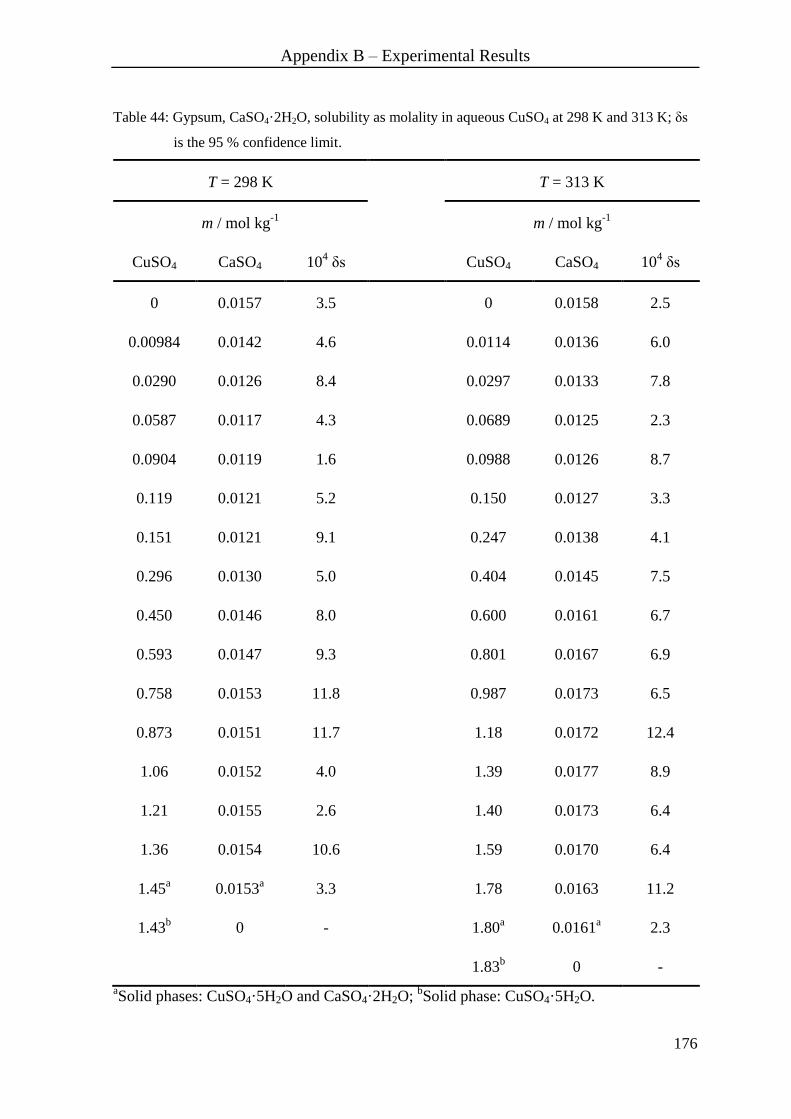
Appendix B – Experimental Results
176
Table 44: Gypsum, CaSO4·2H2O, solubility as molality in aqueous CuSO4 at 298 K and 313 K; δs
is the 95 % confidence limit.
T = 298 K T = 313 K
m / mol kg-1
m / mol kg-1
CuSO4 CaSO4 104 δs CuSO4 CaSO4 10
4 δs
0 0.0157 3.5 0 0.0158 2.5
0.00984 0.0142 4.6 0.0114 0.0136 6.0
0.0290 0.0126 8.4 0.0297 0.0133 7.8
0.0587 0.0117 4.3 0.0689 0.0125 2.3
0.0904 0.0119 1.6 0.0988 0.0126 8.7
0.119 0.0121 5.2 0.150 0.0127 3.3
0.151 0.0121 9.1 0.247 0.0138 4.1
0.296 0.0130 5.0 0.404 0.0145 7.5
0.450 0.0146 8.0 0.600 0.0161 6.7
0.593 0.0147 9.3 0.801 0.0167 6.9
0.758 0.0153 11.8 0.987 0.0173 6.5
0.873 0.0151 11.7 1.18 0.0172 12.4
1.06 0.0152 4.0 1.39 0.0177 8.9
1.21 0.0155 2.6 1.40 0.0173 6.4
1.36 0.0154 10.6 1.59 0.0170 6.4
1.45a
0.0153a
3.3 1.78 0.0163 11.2
1.43b
0 - 1.80a
0.0161a
2.3
1.83b
0 -
aSolid phases: CuSO4·5H2O and CaSO4·2H2O;
bSolid phase: CuSO4·5H2O.

Appendix B – Experimental Results
177
Table 45: Gypsum, CaSO4·2H2O, solubility as molality in aqueous ZnSO4 at 298 K and 313 K; δs
is the 95 % confidence limit.
T = 298 K T = 313 K
m / mol kg-1
m / mol kg-1
ZnSO4 CaSO4 104 δs ZnSO4 CaSO4 10
4 δs
0 0.0157 3.5 0 0.0158 2.5
0.00993 0.0134 5.7 0.00862 0.0146 4.4
0.0246 0.0127 7.0 0.0298 0.0134 3.7
0.0512 0.0115 1.3 0.0570 0.0124 2.1
0.103 0.0117 2.6 0.122 0.0129 7.6
0.250 0.0122 1.8 0.301 0.0145 0.76
0.499 0.0135 1.9 0.611 0.0156 10.5
0.793 0.0146 9.6 1.00 0.0173 5.4
0.914 0.0150 7.5 1.36 0.0169 5.7
1.08 0.0156 11.6 1.83 0.0167 9.9
1.40 0.0153 7.8 2.26 0.0146 4.2
1.69 0.0143 8.4 2.66 0.0134 5.4
2.12 0.0130 7.2 3.07 0.0113 4.5
2.16 0.0135 10.4 3.43 0.00946 1.8
2.46 0.0122 4.9 3.86 0.00786 5.6
2.74 0.0104 2.5 4.12 0.00658 5.8
2.94 0.00961 4.2 4.44c
0.00538c
4.2
3.23 0.00826 3.5 4.34d
0 -
3.60a
0.00651a
1.5
3.53b
0 -
aSolid phases: ZnSO4·7H2O and CaSO4·2H2O;
bSolid phase: ZnSO4·7H2O;
cSolid phases: ZnSO4·6H2O and CaSO4·2H2O;
dSolid phase: ZnSO4·6H2O.

Appendix B – Experimental Results
178
Quaternary System K+, Ca
2+, M
2+ / SO4
2- // H2O (M = Mg, Mn, Co, Ni, Cu, Zn)
Table 46: List of abbreviations of the occurring solid phases.
Abbreviation Formula (M = Mg, Mn, Co, Ni, Cu, Zn) Mineral
Ph K2SO4·MSO4·2CaSO4·2H2O polyhalite
Pi K2SO4·MSO4·6H2O picromerite
Lg K2SO4·2MSO4 langbeinite
G CaSO4·2H2O gypsum
Ep MgSO4·7H2O epsomite
Sz MnSO4·H2O szmikite
Bie CoSO4·7H2O bieberite
Ret -NiSO4·6H2O retgersite
Cha CuSO4·5H2O chalcanthite
Bia ZnSO4·6H2O bianchite
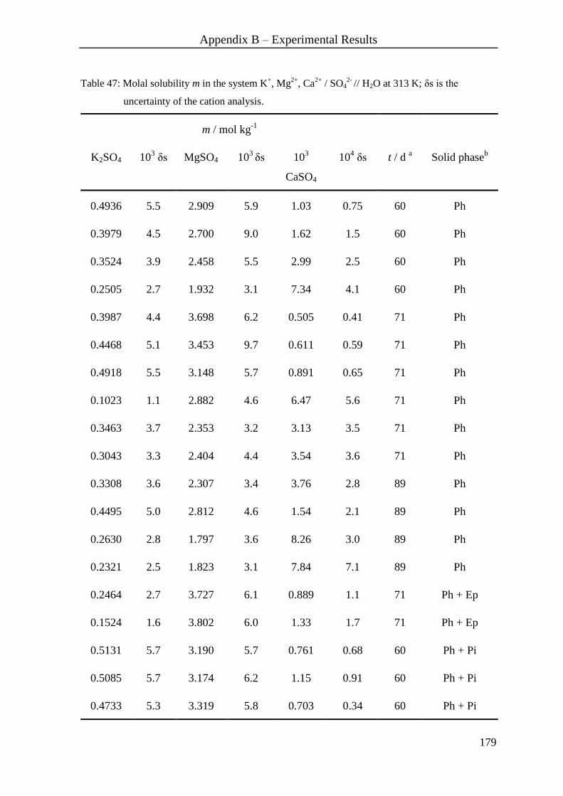
Appendix B – Experimental Results
179
Table 47: Molal solubility m in the system K+, Mg
2+, Ca
2+ / SO4
2- // H2O at 313 K; δs is the
uncertainty of the cation analysis.
m / mol kg-1
K2SO4 103 δs MgSO4 10
3 δs 10
3
CaSO4
104 δs t / d
a Solid phase
b
0.4936 5.5 2.909 5.9 1.03 0.75 60 Ph
0.3979 4.5 2.700 9.0 1.62 1.5 60 Ph
0.3524 3.9 2.458 5.5 2.99 2.5 60 Ph
0.2505 2.7 1.932 3.1 7.34 4.1 60 Ph
0.3987 4.4 3.698 6.2 0.505 0.41 71 Ph
0.4468 5.1 3.453 9.7 0.611 0.59 71 Ph
0.4918 5.5 3.148 5.7 0.891 0.65 71 Ph
0.1023 1.1 2.882 4.6 6.47 5.6 71 Ph
0.3463 3.7 2.353 3.2 3.13 3.5 71 Ph
0.3043 3.3 2.404 4.4 3.54 3.6 71 Ph
0.3308 3.6 2.307 3.4 3.76 2.8 89 Ph
0.4495 5.0 2.812 4.6 1.54 2.1 89 Ph
0.2630 2.8 1.797 3.6 8.26 3.0 89 Ph
0.2321 2.5 1.823 3.1 7.84 7.1 89 Ph
0.2464 2.7 3.727 6.1 0.889 1.1 71 Ph + Ep
0.1524 1.6 3.802 6.0 1.33 1.7 71 Ph + Ep
0.5131 5.7 3.190 5.7 0.761 0.68 60 Ph + Pi
0.5085 5.7 3.174 6.2 1.15 0.91 60 Ph + Pi
0.4733 5.3 3.319 5.8 0.703 0.34 60 Ph + Pi
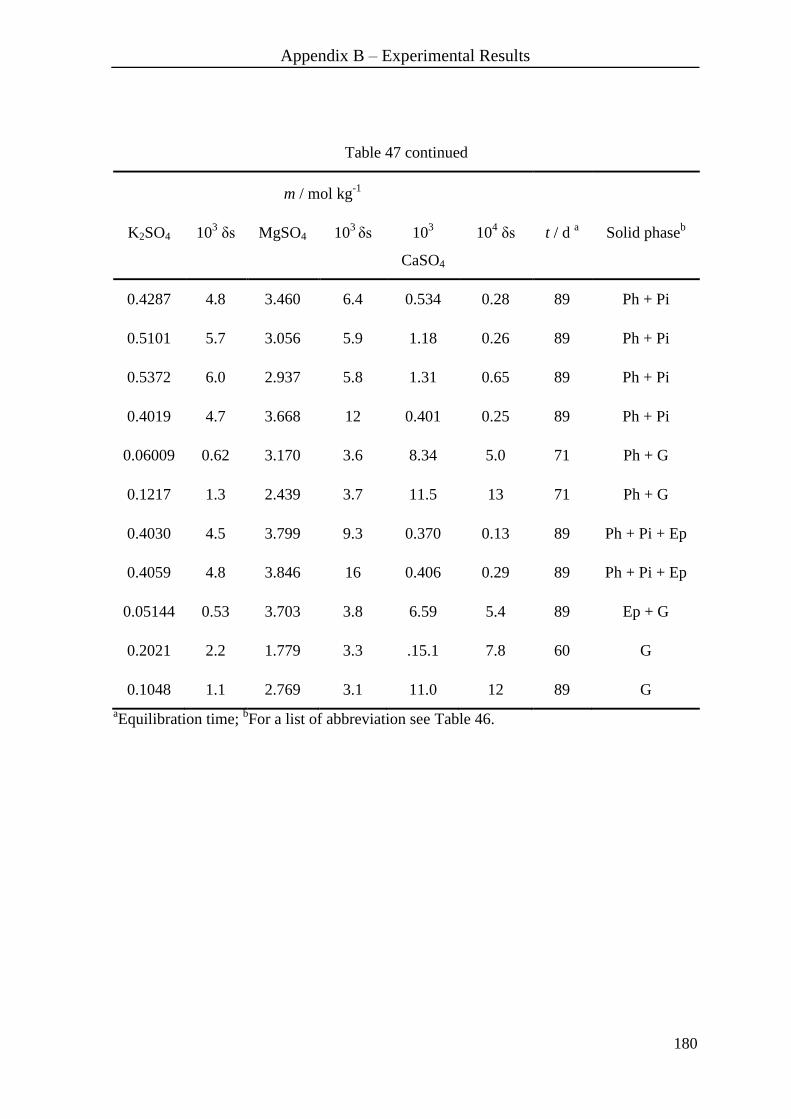
Appendix B – Experimental Results
180
Table 47 continued
m / mol kg-1
K2SO4 103 δs MgSO4 10
3 δs 10
3
CaSO4
104 δs t / d
a Solid phase
b
0.4287 4.8 3.460 6.4 0.534 0.28 89 Ph + Pi
0.5101 5.7 3.056 5.9 1.18 0.26 89 Ph + Pi
0.5372 6.0 2.937 5.8 1.31 0.65 89 Ph + Pi
0.4019 4.7 3.668 12 0.401 0.25 89 Ph + Pi
0.06009 0.62 3.170 3.6 8.34 5.0 71 Ph + G
0.1217 1.3 2.439 3.7 11.5 13 71 Ph + G
0.4030 4.5 3.799 9.3 0.370 0.13 89 Ph + Pi + Ep
0.4059 4.8 3.846 16 0.406 0.29 89 Ph + Pi + Ep
0.05144 0.53 3.703 3.8 6.59 5.4 89 Ep + G
0.2021 2.2 1.779 3.3 .15.1 7.8 60 G
0.1048 1.1 2.769 3.1 11.0 12 89 G
aEquilibration time;
bFor a list of abbreviation see Table 46.
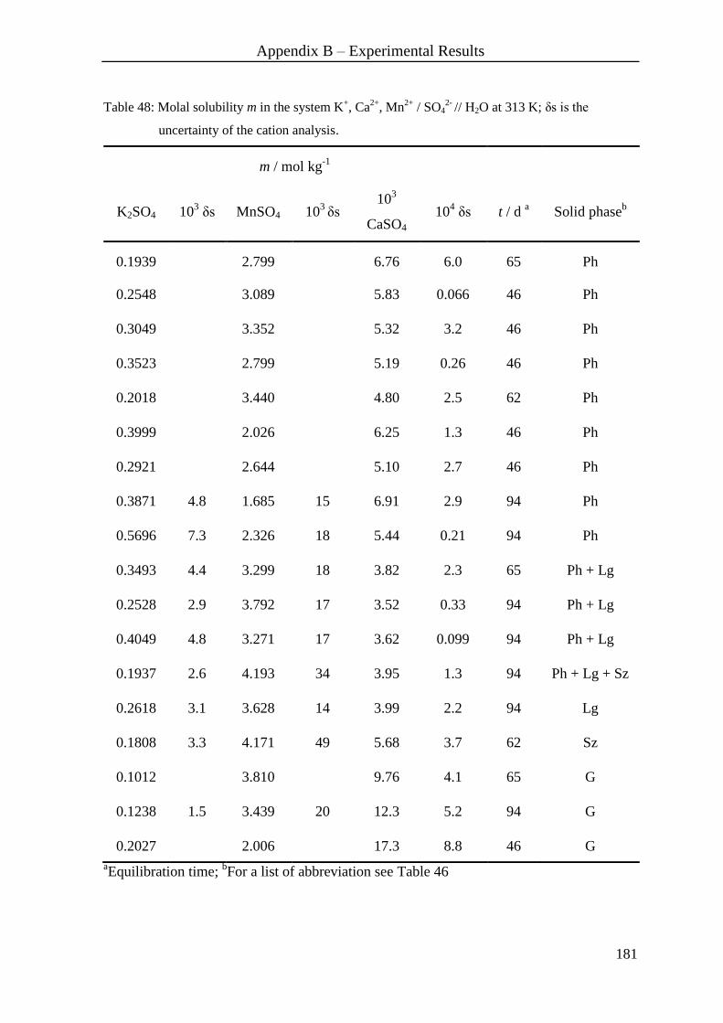
Appendix B – Experimental Results
181
Table 48: Molal solubility m in the system K+, Ca
2+, Mn
2+ / SO4
2- // H2O at 313 K; δs is the
uncertainty of the cation analysis.
m / mol kg-1
K2SO4 103 δs MnSO4 10
3 δs
103
CaSO4 10
4 δs t / d
a Solid phase
b
0.1939 2.799 6.76 6.0 65 Ph
0.2548 3.089 5.83 0.066 46 Ph
0.3049 3.352 5.32 3.2 46 Ph
0.3523 2.799 5.19 0.26 46 Ph
0.2018 3.440 4.80 2.5 62 Ph
0.3999 2.026 6.25 1.3 46 Ph
0.2921 2.644 5.10 2.7 46 Ph
0.3871 4.8 1.685 15 6.91 2.9 94 Ph
0.5696 7.3 2.326 18 5.44 0.21 94 Ph
0.3493 4.4 3.299 18 3.82 2.3 65 Ph + Lg
0.2528 2.9 3.792 17 3.52 0.33 94 Ph + Lg
0.4049 4.8 3.271 17 3.62 0.099 94 Ph + Lg
0.1937 2.6 4.193 34 3.95 1.3 94 Ph + Lg + Sz
0.2618 3.1 3.628 14 3.99 2.2 94 Lg
0.1808 3.3 4.171 49 5.68 3.7 62 Sz
0.1012 3.810 9.76 4.1 65 G
0.1238 1.5 3.439 20 12.3 5.2 94 G
0.2027 2.006 17.3 8.8 46 G
aEquilibration time;
bFor a list of abbreviation see Table 46

Appendix B – Experimental Results
182
Table 49: Molal solubility m in the system K+, Ca
2+, Co
2+ / SO4
2- // H2O at 313 K; δs is the
uncertainty of the cation analysis.
m / mol kg-1
K2SO4 103 δs CoSO4 10
3 δs
103
CaSO4 10
4 δs t / d
a Solid phase
b
0.4042 1.542 3.20 2.0 69 Ph
0.2129 2.624 3.12 1.6 62 Ph
0.2579 2.877 2.17 0.45 46 Ph
0.3074 2.650 2.20 2.1 46 Ph
0.3581 2.064 2.77 0.055 46 Ph
0.1052 2.520 6.77 7.2 94 Ph
0.3061 2.342 3.07 4.9 65 Ph
0.1647 2.133 6.02 2.8 65 Ph
0.3037 1.738 4.15 4.0 65 Ph
0.1997 1.545 6.22 5.1 62 Ph
0.1400 1.6 1.762 7.1 7.30 6.7 89 Ph
0.4917 5.7 1.312 6.5 3.07 1.8 89 Ph
0.3638 4.4 2.456 14 1.57 0.026 69 Ph + Pi
0.4121 5.0 2.002 13 1.64 0.85 69 Ph + Pi
0.3143 3.7 2.907 13 2.24 1.1 72 Ph + Pi
0.3470 4.4 2.785 21 1.54 0.20 72 Ph + Pi
0.1012 1.2 2.995 14 3.78 4.2 94 Ph + Bie
0.1927 2.3 3.060 14 1.91 0.030 94 Ph + Bie
0.1054 1.800 17.5 3.1 65 G
aEquilibration time;
bFor a list of abbreviation see Table 46

Appendix B – Experimental Results
183
Table 50: Molal solubility m in the system K+, Ca
2+, Ni
2+ / SO4
2- // H2O at 313 K; δs is the
uncertainty of the cation analysis.
m / mol kg-1
K2SO4 103 δs NiSO4 10
3 δs
103
CaSO4 10
4 δs t / d
a Solid phase
b
0.1040 1.6 3.151 48 10.1 3.1 89 G + Pi + Ret
0.1374 1.9 2.401 33 14.8 9.1 89 G + Pi
0.1332 1.8 1.840 24 19.6 1.1 74 G
0.1020 2.763 12.1 4.7 74 G
0.1519 1.450 18.4 8.3 46 G
0.1563 1.255 18.2 1.8 46 G
0.1267 1.497 17.7 1.2 46 G
0.1021 1.4 2.084 28 15.4 7.1 64 G
0.1047 1.083 17.3 1.5 92 G
0.1619 0.550 16.2 1.2 92 G
0.1239 1.8 2.770 40 8.66 7.1 74 Pi
0.2036 2.5 1.066 13 5.33 3.1 64 Pi
0.1608 2.1 1.854 24 8.57 5.9 64 Pi
0.1723 0.84 1.630 8.0 7.54 2.1 92 Pi
aEquilibration time;
bFor a list of abbreviation see Table 46

Appendix B – Experimental Results
184
Table 51: Molal solubility m in the system K+, Ca
2+, Cu
2+ / SO4
2- // H2O at 313 K; δs is the
uncertainty of the cation analysis.
m / mol kg-1
K2SO4 103 δs CuSO4 10
3 δs
103
CaSO4 10
4 δs t / d
a Solid phase
b
0.2541 2.7 1.815 0.93 0.512 0.26 74 Ph
0.2583 1.555 0.629 0.81 74 Ph
0.3644 1.041 0.634 0.062 46 Ph
0.3191 1.476 0.549 0.32 46 Ph
0.3152 1.266 0.614 0.23 46 Ph
0.08817 1.009 2.41 0.057 92 Ph
0.2122 1.332 0.913 0.49 71 Ph
0.1020 1.320 1.88 0.93 84 Ph
0.2087 1.044 1.07 0.34 84 Ph
0.3171 0.7786 0.755 0.032 84 Ph
0.3855 0.6775 0.473 0.20 89 Ph
0.4427 5.2 1.020 6.9 0.371 0.17 61 Ph + Pi
0.3945 4.5 1.276 6.5 0.475 0.46 61 Ph + Pi
0.3622 4.2 1.721 8.5 0.398 0.35 61 Ph + Pi
0.3470 4.0 1.867 7.9 0.425 0.27 61 Ph + Pi
0.3180 4.0 1.965 15 0.369 0.17 73 Ph + Cha
0.09407 1.1 1.900 9.1 1.25 0.49 92 Ph + Cha
0.2021 2.4 1.896 13 0.651 0.60 71 Ph + Cha
0.2742 3.2 1.903 9.9 0.437 0.23 89 Ph + Cha
0.1573 1.9 1.919 13 0.950 0.39 71 Cha
aEquilibration time;
bFor a list of abbreviation see Table 46

Appendix B – Experimental Results
185
Table 52: Molal solubility m in the system K+, Ca
2+, Zn
2+ / SO4
2- // H2O at 313 K; δs is the
uncertainty of the cation analysis.
m / mol kg-1
K2SO4 103 δs ZnSO4 10
3 δs 10
3 CaSO4 10
4 δs t / d
a Solid phase
b
0.1491 3.525 1.26 0.080 65 Ph
0.09720 3.050 3.02 0.25 65 Ph
0.1450 2.254 3.74 3.0 65 Ph
0.2509 2.059 2.71 1.9 46 Ph
0.3024 1.768 2.70 0.50 46 Ph
0.2488 1.511 3.65 0.19 46 Ph
0.09640 2.122 7.43 0.18 92 Ph
0.2044 2.807 1.75 1.3 65 Ph
0.2035 1.797 4.03 1.8 65 Ph
0.2139 1.069 5.63 3.0 64 Ph
0.1461 1.263 6.87 0.43 64 Ph
0.09600 1.443 8.67 0.69 64 Ph
0.3775 4.3 1.255 5.9 2.75 0.19 90 Ph
0.2782 3.1 0.9800 5.4 3.71 2.6 90 Ph
0.1179 1.3 0.7640 4.4 9.57 4.7 90 Ph
0.2416 2.9 3.031 16 1.17 0.52 79 Ph + Pi
0.2047 2.4 3.547 15 0.793 0.51 79 Ph + Pi
0.2684 3.3 2.804 18 1.46 0.60 65 Ph + Pi
0.09369 1.1 4.363 20 0.588 0.19 92 Ph + Bia
0.1528 1.9 4.374 28 0.507 0.071 92 Ph + Bia
aEquilibration time;
bFor a list of abbreviation see Table 46
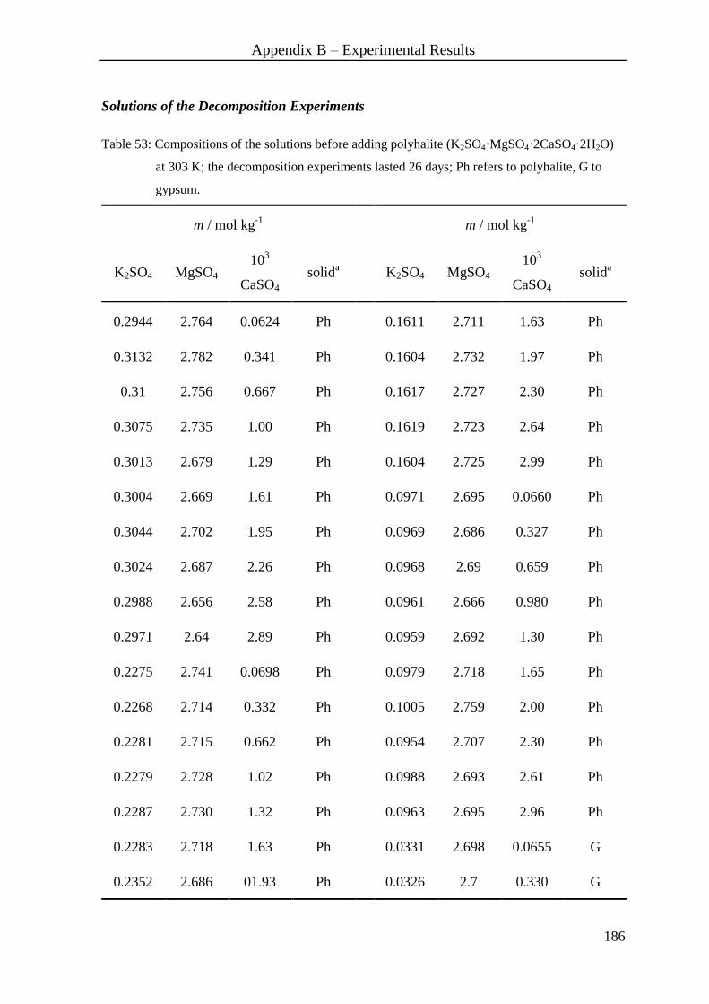
Appendix B – Experimental Results
186
Solutions of the Decomposition Experiments
Table 53: Compositions of the solutions before adding polyhalite (K2SO4·MgSO4·2CaSO4·2H2O)
at 303 K; the decomposition experiments lasted 26 days; Ph refers to polyhalite, G to
gypsum.
m / mol kg-1
m / mol kg-1
K2SO4 MgSO4 10
3
CaSO4 solid
a K2SO4 MgSO4
103
CaSO4 solid
a
0.2944 2.764 0.0624 Ph 0.1611 2.711 1.63 Ph
0.3132 2.782 0.341 Ph 0.1604 2.732 1.97 Ph
0.31 2.756 0.667 Ph 0.1617 2.727 2.30 Ph
0.3075 2.735 1.00 Ph 0.1619 2.723 2.64 Ph
0.3013 2.679 1.29 Ph 0.1604 2.725 2.99 Ph
0.3004 2.669 1.61 Ph 0.0971 2.695 0.0660 Ph
0.3044 2.702 1.95 Ph 0.0969 2.686 0.327 Ph
0.3024 2.687 2.26 Ph 0.0968 2.69 0.659 Ph
0.2988 2.656 2.58 Ph 0.0961 2.666 0.980 Ph
0.2971 2.64 2.89 Ph 0.0959 2.692 1.30 Ph
0.2275 2.741 0.0698 Ph 0.0979 2.718 1.65 Ph
0.2268 2.714 0.332 Ph 0.1005 2.759 2.00 Ph
0.2281 2.715 0.662 Ph 0.0954 2.707 2.30 Ph
0.2279 2.728 1.02 Ph 0.0988 2.693 2.61 Ph
0.2287 2.730 1.32 Ph 0.0963 2.695 2.96 Ph
0.2283 2.718 1.63 Ph 0.0331 2.698 0.0655 G
0.2352 2.686 01.93 Ph 0.0326 2.7 0.330 G
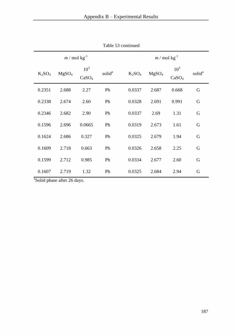
Appendix B – Experimental Results
187
Table 53 continued
m / mol kg-1
m / mol kg-1
K2SO4 MgSO4 10
3
CaSO4 solid
a K2SO4 MgSO4
103
CaSO4 solid
a
0.2351 2.688 2.27 Ph 0.0337 2.687 0.668 G
0.2338 2.674 2.60 Ph 0.0328 2.691 0.991 G
0.2346 2.682 2.90 Ph 0.0337 2.69 1.31 G
0.1596 2.696 0.0665 Ph 0.0319 2.673 1.61 G
0.1624 2.686 0.327 Ph 0.0325 2.679 1.94 G
0.1609 2.718 0.663 Ph 0.0326 2.658 2.25 G
0.1599 2.712 0.985 Ph 0.0334 2.677 2.60 G
0.1607 2.719 1.32 Ph 0.0325 2.684 2.94 G
aSolid phase after 26 days.

Appendix B – Experimental Results
188
Table 54: Compositions of the solutions before adding polyhalite (K2SO4·MgSO4·2CaSO4·2H2O)
at 303 K; the decomposition experiments lasted 50 days; Ph refers to polyhalite, G to
gypsum.
m / mol kg-1
m / mol kg-1
K2SO4 MgSO4 10
3
CaSO4 solid
a K2SO4 MgSO4
103
CaSO4 solid
a
0.3058 2.558 0.0910 Ph 0.1668 2.490 1.73 Ph
0.3204 2.494 0.345 Ph 0.1664 2.486 2.08 Ph
0.3191 2.483 0.702 Ph 0.1662 2.486 2.43 Ph
0.3189 2.480 1.02 Ph 0.1674 2.488 2.78 Ph
0.3197 2.486 1.35 Ph 0.1670 2.505 3.13 Ph
0.3181 2.475 1.68 Ph 0.1003 2.489 0.0725 Ph
0.3200 2.486 2.04 Ph 0.1007 2.485 0.348 Ph
0.3179 2.471 2.37 Ph 0.1002 2.475 0.717 Ph
0.3183 2.478 2.69 Ph 0.1001 2.477 1.03 Ph
0.3154 2.455 3.07 Ph 0.1007 2.483 1.35 Ph
0.2365 2.524 0.0748 Ph 0.1000 2.472 1.66 Ph
0.2354 2.534 0.355 Ph 0.1001 2.474 2.06 Ph
0.2355 2.525 0.715 Ph 0.1001 2.461 2.40 Ph
0.2353 2.531 1.05 Ph 0.0999 2.473 2.75 Ph
0.2376 2.549 1.33 Ph 0.0995 2.461 3.10 Ph
0.2369 2.539 1.72 Ph 0.0334 2.472 0.0756 G
0.2468 2.466 2.06 Ph 0.0340 2.475 0.340 G

Appendix B – Experimental Results
189
Table 54 continued
m / mol kg-1
m / mol kg-1
K2SO4 MgSO4 10
3
CaSO4 solid
a K2SO4 MgSO4
103
CaSO4 solid
a
0.2457 2.460 2.41 Ph 0.0340 2.464 0.689 G
0.4201 4.198 4.63 Ph 0.0339 2.464 1.02 G
0.2459 2.458 3.08 Ph 0.0341 2.468 1.35 G
0.1668 2.514 0.0748 Ph 0.0336 2.453 1.69 G
0.1669 2.505 0.351 Ph 0.0336 2.450 2.06 G
0.1670 2.498 0.697 Ph 0.0339 2.444 2.39 G
0.1664 2.497 1.05 Ph 0.0335 2.442 2.74 G
0.1681 2.489 1.36 Ph 0.0334 2.438 3.07 G
aSolid phase after 50 days.
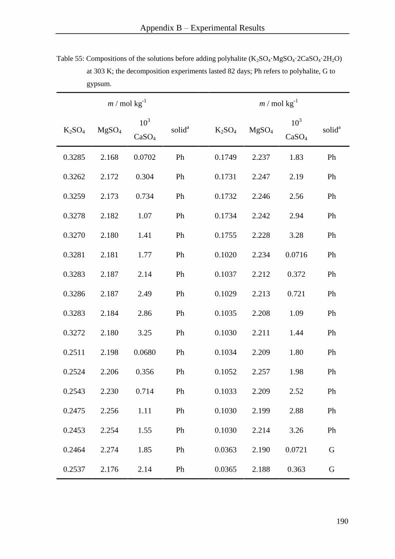
Appendix B – Experimental Results
190
Table 55: Compositions of the solutions before adding polyhalite (K2SO4·MgSO4·2CaSO4·2H2O)
at 303 K; the decomposition experiments lasted 82 days; Ph refers to polyhalite, G to
gypsum.
m / mol kg-1
m / mol kg-1
K2SO4 MgSO4 10
3
CaSO4 solid
a K2SO4 MgSO4
103
CaSO4 solid
a
0.3285 2.168 0.0702 Ph 0.1749 2.237 1.83 Ph
0.3262 2.172 0.304 Ph 0.1731 2.247 2.19 Ph
0.3259 2.173 0.734 Ph 0.1732 2.246 2.56 Ph
0.3278 2.182 1.07 Ph 0.1734 2.242 2.94 Ph
0.3270 2.180 1.41 Ph 0.1755 2.228 3.28 Ph
0.3281 2.181 1.77 Ph 0.1020 2.234 0.0716 Ph
0.3283 2.187 2.14 Ph 0.1037 2.212 0.372 Ph
0.3286 2.187 2.49 Ph 0.1029 2.213 0.721 Ph
0.3283 2.184 2.86 Ph 0.1035 2.208 1.09 Ph
0.3272 2.180 3.25 Ph 0.1030 2.211 1.44 Ph
0.2511 2.198 0.0680 Ph 0.1034 2.209 1.80 Ph
0.2524 2.206 0.356 Ph 0.1052 2.257 1.98 Ph
0.2543 2.230 0.714 Ph 0.1033 2.209 2.52 Ph
0.2475 2.256 1.11 Ph 0.1030 2.199 2.88 Ph
0.2453 2.254 1.55 Ph 0.1030 2.214 3.26 Ph
0.2464 2.274 1.85 Ph 0.0363 2.190 0.0721 G
0.2537 2.176 2.14 Ph 0.0365 2.188 0.363 G
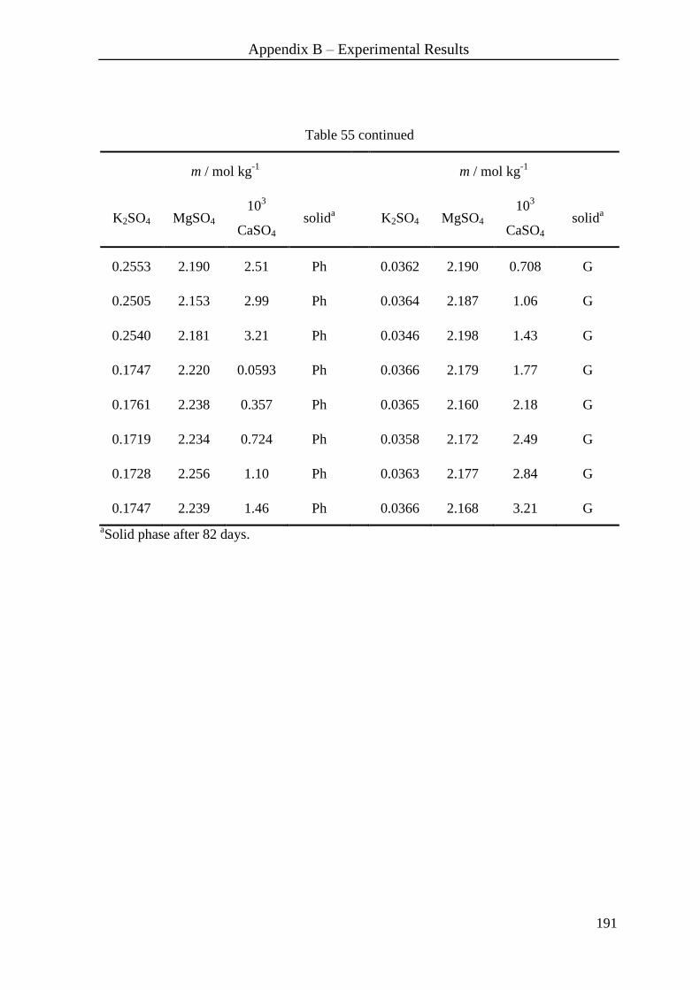
Appendix B – Experimental Results
191
Table 55 continued
m / mol kg-1
m / mol kg-1
K2SO4 MgSO4 10
3
CaSO4 solid
a K2SO4 MgSO4
103
CaSO4 solid
a
0.2553 2.190 2.51 Ph 0.0362 2.190 0.708 G
0.2505 2.153 2.99 Ph 0.0364 2.187 1.06 G
0.2540 2.181 3.21 Ph 0.0346 2.198 1.43 G
0.1747 2.220 0.0593 Ph 0.0366 2.179 1.77 G
0.1761 2.238 0.357 Ph 0.0365 2.160 2.18 G
0.1719 2.234 0.724 Ph 0.0358 2.172 2.49 G
0.1728 2.256 1.10 Ph 0.0363 2.177 2.84 G
0.1747 2.239 1.46 Ph 0.0366 2.168 3.21 G
aSolid phase after 82 days.

Appendix B – Experimental Results
192
Enthalpies of Dissolution of the Polyhalites
Table 56: Integral molar heat of dissolution of Mg-polyhalite in aqueous NaClO4 solution at 298 K.
Mg-polyhalite NaClO4 solution
m / 103 g m / g m / mol kg
-1 solH / kJ mol
-1
98.428 103.372 0.517 -28.21
98.614 103.379 0.517 -28.67
98.630 103.353 0.517 -28.38
100.602 106.204 0.879 -33.32
97.876 106.158 0.879 -33.05
100.778 109.281 1.30 -38.26
94.766 109.528 1.30 -38.14
101.853 112.171 1.75 -41.96
100.846 112.433 1.75 -42.34
101.013 114.268 2.05 -44.49
93.745 114.232 2.05 -44.57

Appendix B – Experimental Results
193
Table 57: Integral molar heat of dissolution of Mn-polyhalite in aqueous NaClO4 solution at 298 K.
Mn-polyhalite NaClO4 solution
m / 103 g m / g m / mol kg
-1 solH / kJ mol
-1
98.099 103.332 0.491 -27.56
99.294 103.360 0.491 -27.95
99.312 106.534 0.908 -34.30
95.485 106.475 0.908 -34.10
98.789 109.710 1.41 -37.83
97.284 109.740 1.41 -38.59
97.493 109.897 1.41 -38.32
99.626 112.354 1.80 -41.85
100.094 112.000 1.80 -41.64
100.029 112.539 1.80 -42.23
98.420 114.966 2.23 -44.72
100.299 115.031 2.23 -44.54
100.201 115.014 2.23 -44.88

Appendix B – Experimental Results
194
Table 58: Integral molar heat of dissolution of Co-polyhalite in aqueous NaClO4 solution at 298 K.
Co-polyhalite NaClO4 solution
m / 103 g m / g m / mol kg
-1 solH / kJ mol
-1
95.504 103.460 0.445 -20.690
98.680 103.341 0.445 -20.652
99.056 103.442 0.445 -20.263
98.706 106.559 0.908 -26.649
98.790 106.587 0.908 -26.405
93.371 109.552 1.39 -31.110
100.946 109.529 1.39 -31.366
96.296 112.321 1.75 -35.003
96.338 112.559 1.75 -35.125
95.721 114.212 2.05 -36.149
93.348 114.164 2.05 -35.812

Appendix B – Experimental Results
195
Table 59: Integral molar heat of dissolution of Ni-polyhalite in aqueous NaClO4 solution at 298 K.
Ni-polyhalite NaClO4 solution
m / 103 g m / g m / mol kg
-1 solH / kJ mol
-1
100.565 103.477 0.517 -26.15
100.979 103.492 0.517 -26.56
99.561 103.494 0.517 -26.37
100.366 106.112 0.879 -31.55
100.274 106.147 0.879 -31.23
100.432 106.120 0.879 -31.93
100.338 109.266 1.30 -36.54
97.427 108.818 1.30 -36.73
100.344 109.319 1.30 -36.27
97.713 112.223 1.75 -40.67
99.593 112.316 1.75 -40.33
100.089 114.221 2.05 -42.16
99.622 114.034 2.05 -42.46
97.615 114.071 2.05 -42.49
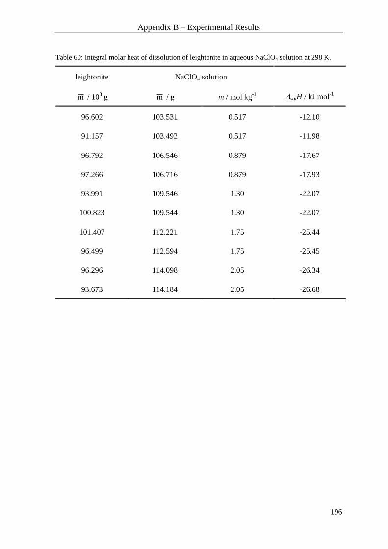
Appendix B – Experimental Results
196
Table 60: Integral molar heat of dissolution of leightonite in aqueous NaClO4 solution at 298 K.
leightonite NaClO4 solution
m / 103 g m / g m / mol kg
-1 solH / kJ mol
-1
96.602 103.531 0.517 -12.10
91.157 103.492 0.517 -11.98
96.792 106.546 0.879 -17.67
97.266 106.716 0.879 -17.93
93.991 109.546 1.30 -22.07
100.823 109.544 1.30 -22.07
101.407 112.221 1.75 -25.44
96.499 112.594 1.75 -25.45
96.296 114.098 2.05 -26.34
93.673 114.184 2.05 -26.68

Appendix B – Experimental Results
197
Table 61: Integral molar heat of dissolution of Zn-polyhalite in aqueous NaClO4 solution at 298 K.
Zn-polyhalite NaClO4 solution
m / 103 g m / g m / mol kg
-1 solH / kJ mol
-1
97.870 103.422 0.517 -25.84
99.756 103.491 0.517 -26.61
98.653 103.458 0.517 -26.14
96.331 106.241 0.879 -31.33
99.552 106.101 0.879 -31.32
92.684 109.310 1.30 -36.59
95.938 109.140 1.30 -36.91
99.729 109.182 1.41 -37.32
97.813 112.221 1.75 -40.16
97.523 112.129 1.75 -40.46
99.114 112.504 1.80 -40.82
98.654 114.047 2.05 -42.26
95.452 114.189 2.05 -42.16

Appendix C – Temperature-Dependent Parameters
198
Appendix C – Temperature-Dependent Parameters
The temperature-dependent equation used was as follows.
2
2lnT
FETDTTCB
T
AP
Table 62: Binary temperature-dependent Pitzer parameters of MnSO4;
valid between 283 K to 323 K.
0
MX 1
MX 2
MX MXC
A 0 0 0 0
B -1.1260124·10
-
1
6.7952664·10-1
132.713272 2.2443503·10-1
C 0 0 0 0
D 1.07027·10-3
7.61889·10-3
-5.7928315·10
-
1
-6.9789·10-4
E 0 0 0 0
F 0 0 0 0
Table 63: Temperature dependence of solubility constants lnKsol of MnSO4·5H2O, MnSO4·4H2O
and MnSO4·H2O; valid between 283 K to 323K.
MnSO4·5H2O MnSO4·4H2O MnSO4·H2O
A 106.287754 2273.16463 5141.68190
B 2232.85467 -11.1782315 -20.2762856
C -536.699629 0 0
D 3.71781412 0 0
E -3.23429120·10-3
0 0
F 3.18172223 0 0

Appendix C – Temperature-Dependent Parameters
199
Table 64: Binary temperature-dependent Pitzer parameters of CoSO4;
valid between 283 K to 323 K.
0
MX 1
MX 2
MX MXC
A 0 0 0 0
B 9.876806·10-2
-1.81211963 51.2228194 5.29455·10-2
C 0 0 0 0
D
3.2897·10-4
1.546221·10-2
-3.6868668·10-
1 -9.9521·10
-5
E 0 0 0 0
F 0 0 0 0
Table 65: Temperature dependence of solubility constants lnKsol of CoSO4·7H2O, and
CoSO4·6H2O; valid between 283 K to 323K.
CoSO4·7H2O CoSO4·6H2O
A -927.919024 -252.573848
B -3.07994623 -4.21786316
C 0 0
D 0 0
E 8.90261402·10-6
0
F 0 0
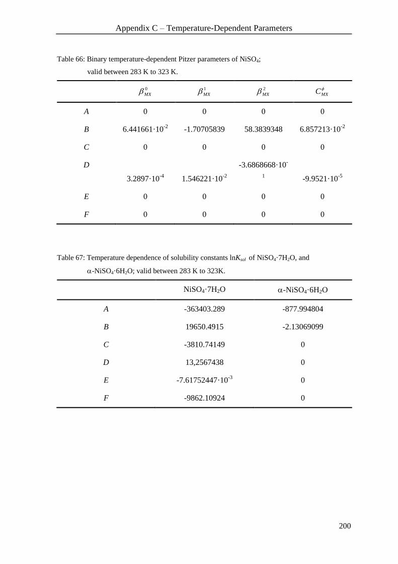
Appendix C – Temperature-Dependent Parameters
200
Table 66: Binary temperature-dependent Pitzer parameters of NiSO4;
valid between 283 K to 323 K.
0
MX 1
MX 2
MX MXC
A 0 0 0 0
B 6.441661·10-2
-1.70705839 58.3839348 6.857213·10-2
C 0 0 0 0
D
3.2897·10-4
1.546221·10-2
-3.6868668·10-
1 -9.9521·10
-5
E 0 0 0 0
F 0 0 0 0
Table 67: Temperature dependence of solubility constants lnKsol of NiSO4·7H2O, and
-NiSO4·6H2O; valid between 283 K to 323K.
NiSO4·7H2O -NiSO4·6H2O
A -363403.289 -877.994804
B 19650.4915 -2.13069099
C -3810.74149 0
D 13,2567438 0
E -7.61752447·10-3
0
F -9862.10924 0

Appendix C – Temperature-Dependent Parameters
201
Table 68: Binary temperature-dependent Pitzer parameters of CuSO4;
valid between 283 K to 323 K.
0
MX 1
MX 2
MX MXC
A 0 0 0 0
B
5.9625351·10-1
-2.36822573 93.6250332
-3.8305932·10-
1
C 0 0 0 0
D
-1.27011·10-3
1.675062·10-2
-5.0265414·10-
1 1.33093·10
-3
E 0 0 0 0
F 0 0 0 0
Table 69: Temperature dependence of solubility constants lnKsol of CuSO4·5H2O; valid between
283 K to 323K.
CuSO4·5H2O
A 454733.065
B -24875.2352
C 4834.20937
D -17,0839760
E 1.00578216·10-2
F 10328.3053

Appendix C – Temperature-Dependent Parameters
202
Table 70: Binary temperature-dependent Pitzer parameters of ZnSO4;
valid between 283 K to 323 K.
0
MX 1
MX 2
MX MXC
A 0 0 0 0
B -1.2339188·10-
1 -3.876447·10
-1 36.4036876 2.0700838·10
-1
C 0 0 0 0
D
1.03402·10-3
1.123275·10-2
-3.0939791·10-
1 -5.8564·10
-4
E 0 0 0 0
F 0 0 0 0
Table 71: Temperature dependence of solubility constants lnKsol of ZnSO4·7H2O and ZnSO4·6H2O;
valid between 283 K to 323K.
ZnSO4·7H2O ZnSO4·6H2O
A -1569.56605 192.437218
B 8.43350341·10-1
-4.63543759
C 0 0
D 0 0
E 0 0
F 0 0

Versicherung
203
Versicherung
Hiermit versichere ich, dass ich die vorliegende Arbeit ohne unzulässige Hilfe Dritter und
ohne Benutzung anderer als der angegebenen Hilfsmittel angefertigt habe; die aus fremden
Quellen direkt oder indirekt übernommenen Gedanken sind als solche kenntlich gemacht.
Bei der Auswahl und Auswertung des Materials sowie bei der Herstellung des Manuskripts
habe ich Unterstützungsleistungen von folgender Person erhalten:
Prof. Dr. rer. nat. Wolfgang Voigt
Weitere Personen waren an der Abfassung der vorliegenden Arbeit nicht beteiligt. Die
Hilfe eines Promotionsberaters habe ich nicht in Anspruch genommen. Weitere Personen
haben von mir keine geldwerten Leistungen für Arbeiten erhalten, die nicht als solche
kenntlich gemacht worden sind.
Die Arbeit wurde bisher weder im Inland noch im Ausland in gleicher oder ähnlicher Form
einer anderen Prüfungsbehörde vorgelegt.
Freiberg, 25.08.2009

Danksagung
204
Danksagung
So eine Arbeit wird eigentlich nie fertig,
man muss sie für fertig erklären,
wenn man nach der Zeit und den Umständen das Möglichste getan hat.
Johann Wolfgang von Goethe
Mit diesem Ausspruch von J. W. Goethe möchte ich mich bei Prof. W. Voigt für das stete
Interesse am Fortgang der Arbeit und die Möglichkeiten, mich mit anderen
Wissenschaftlern auszutauschen, bedanken. So konnte ich durch einen Aufenthalt in Israel
und bei verschiedenen Konferenzen Kontakte knüpfen und ausbauen. Des Weiteren ist die
Realisierung der durchgehenden finanziellen Unterstützung meiner Promotion durch Prof.
W. Voigt nicht als selbstverständlich zu betrachten.
Der Arbeitsgruppe von Prof. W. Klemm (Dr. A. Pleßow) insbesondere G. Bombach und B.
Düsing danke ich für die ausdauernde Hilfe während dem Erstellen der Methode für die
Calciumanalytik. Trotz der Zugehörigkeit zu einer anderen Fakultät nahmen sie sich die
Zeit, mir mit Rat und Tat zur Seite zu stehen, und schafften eine angenehme und
produktive Arbeitsatmosphäre.
In gleicher Weise möchte ich mich an dieser Stelle bei verschiedenen Mitarbeitern des
Instituts für Physikalische Chemie bedanken. Dr. J. Seidel und D. Süßner standen mir
tatkräftig und unermüdlich bei den kalorimetrischen Messungen zur Seite. Außerdem
sollen hier Dr. R. Kirchner und A. Lißner erwähnt werden, die mir bei den Arbeiten mit
MATLAB immer wieder über Probleme hinweggeholfen haben.
Prof. P. Williams danke ich besonders für seine unerwartete Hilfe bei der Fertigstellung
des Manuskriptes, durch sein Korrekturlesen machte er mir verschiedene Feinheiten der
englischen Sprache zugänglich.

Danksagung
205
Für die vielen kleinen und großen Hilfestellungen sowie für die familiäre Atmosphäre
danke ich der Arbeitsgruppe Salze von Prof. W. Voigt. Besonders sind dabei R. Mossig, S.
Fritz, C. Rissom und C. Voigt zu erwähnen. Da es nicht immer nur die fachlichen
Hilfestellungen sind, die einem weiterhelfen, sondern oft auch ein freundschaftliches
Gespräch oder ein Klaps auf die Schulter.
Meiner Familie und meinem Freund Dirk Wählisch danke ich für die Geduld und
Unterstützung während der Arbeit. Das Verständnis meines Freundes und sein Ansporn
weiter zu machen, wenn sich mal wieder ein unüberwindlich geglaubtes Problem auftat,
kann ich nicht hoch genug bewerten.
Eine Arbeit entsteht nicht allein und im „dunklen Kämmerlein“, es bedarf dazu der
Anregung, Hilfe, Diskussion und manchmal der Geduld verschiedener Personen. In diesem
Sinne bedanke ich mich bei jedem der am Gelingen meiner Dissertation beteiligt war.