"

..

CRUDE, DI'RECT AND I.NDlRECT STANDARDIZED RATES:WHI'CH (IF ANY) SHOULD BE USED?

by

Regina C. E1andt-Johnson

Department of BiostatisticsUnivers'ity of NorthCaro1ina at Chapel Hill

Institute of S'tatistics Mimeo Series No. 1414

August 1982

CRUDE, DIRECT AND INDIRECT STANDARDIZED RATES:WHICH (IF ANY) SHOULD BE USED?

Regina C. Elandt-JohnsonDepartment of Biostatistics, University of North Carolina

Chapel Hill, NIX. U.S.A.

SUMMARY

Direct and indirect standardizations are briefly reviewed, emphasizing

their validity under a multiplicative model without interaction of age specific

rates, in accordance with Freeman and Holford (1980). It is shown that when the

proportionate age distributions in the study and standard populations are the

same, crude ra~es can be used (Section 2). This is also required for internal

standardization (Section 5). The paper is mainly concerned with the interpre-

tation and use of standardized rates, with special reference to hypothesis testing.

Two important situations are distinguished: (i) data represent complete popu-

elations; (ii) data represent samples. No meaningful test is needed in situation

(i), but some possible indicators of the fit of a model are discussed (Section 3).

Their use is illustrated in searching for declining trend in mortality from

Ischemic Heart Disease in U.S. White Males over period 1968~77 (Example 1).

Testing for heterogeneity among different clinics (samples) using a multiplicative

Poisson model is discussed in Section 4 and Example 2. Contrary to the con-

elusion of Freeman and Holford (1980), indirect standardization -- more precisely,

the use of standardized mortality ratios -- rather than direct standardization is

here favored, because of the interpretation of data being fitted to a model.

Formally, however, expected values of indirect and direct standardized rates are

the same, provided a multiplicative model without interaction is valid, . so

that either form of standardization leads to the same conlusion.

2

Keywords: Age specific, crude and adjusted rates; Direct and indirect

standardized rates; External and internal standardization; Multiplicative

models; Interaction; Ischemic Heart Disease; Follow-up studies.

This work was supported by U.S. National Heart, Lung, and Blood

. Institute contract NIH-NHLI-7l2243 from the National Institutes of Health.

3

1. INTRODUCTION

1.1. Suppose we are interested i~ comparison of incidence functionsI

of a certain event occurring in G distinct groups of individuals, each group

subclassified into I strata determined by levels of a certain characterisic.

For convenience, assume that the event under consideration is death, and we

wish to compare mortality patterns of G populations over I age strata.

A useful technique, at the initial stage of analysis, is to display

age specific rates as functions of age and compare them graphically. Further,

survival functions can be evaluated and compared. It is, however, customary

in epidemiological research to seek for a single summary index for each

population which includes as much as possible of the information on mortality,

and to use these indices as a kind of "test statistic" in comparative analysis.

~ The indices customarily used by epidemiologists are: overall or crude rate;

age adjusted or directly standardized rate; and standardized mortality ratio

(SMR) or the latter multiplied by the crude rate for the standard population

often referred to as the indirectly standardized rate.

Suppose that data were collected over a fixed period T. For the gth

population and the ith stratum, let N . denote the midperiod populationgl.

exposed to risk, Dgi - the number of deaths, and A • = D ilN . - the cor-gl. g gl.

responding age specific death rate (per person per year of life) over

period T. For a model or standard population (S), the corresponding quantities

are: NSi ' DSi ' ASi ' etc.

We use the customary notation for sums:I G

Ng . = IN., D. i = I Dgi , etc.i=l gl. g=l

4

ILet W i = N i/N ,with L W . = 1, represent the proportionate age

g. g g. g=l g~

distribution in the gth population, and similarly, let wSi = NSi/NS• be the

corresponding (proportionate) age distribution in the standard population.

1.2. For the gthpopulation, the following summary indices can

be defined:

(i) The overall or crude rate,

A(C) =g

IL W ).,

i=l gi g-i

-1 I= N L N i A • = D INg. i=l g g~ g. g.

(1.1)

(ii) The age-adjusted or directly standardized rate,

A(DS) =g

I I~ -1 ~ AL VlSi A . =- NS • L NSi · •

i=l g~ i=l· g~(1.2)

(iii) The indirectly standardized rate,

where

ILvi. A •

i=l g~ g~

IL w i A..••

i=l g s~

I

Li=l

Dw A(C)=~ A(C)

Si S1 E S'g.(1.3)

Here

Eg. =IL Egii=l

(1.4)

(1.5)

i~ the expected number of deaths in the ith stratum, under the null hypothesis

that the standard population (S) is the correct mortality model, and E is ~g.

5

the total number of expected deaths under this model. The ratio,

D IE = (SMR) ,g. g. g

called the standardized mortality ratio (SMR), is, in fact, used more

(1.6)

commonly by epidemiologists than the indirectly standardized rate (1.3),

which may now be simply expressed in the form

>.(IS)g

= (SMR) >. (C)g S (1.3a)

1.3. It has been realized for a long time that the crude rates may

give invalid comparisons since their values may be affected by differences

in age compositions of the compared populations. Adjustment by using age

distribution of a standard population (direct standardization) was introduced

to remove this effect. This procedure, however, has some pitfalls of its

own; the values of age adjusted rates, and their comparisons depend on the

composition of the standard population used. Earlier publications on this

topic were mainly concerned with the choice of the standard population

(e.g. Kitagawa (1964), Spiegelman and Marks (1966»,or searching for indices

other than directly standardized rates (Yerushalmy (1951), Kitagawa (1966»).

Despite criticism, age adjusted rates are still in common use,

especially in the analysis of long-term mortality trends in chronic diseases.

For example, age adjusted rates have been used recently in the analysis of

trends in cardiovascular mortality (in: Proceedings (1979». Also,

Doll and Peto (1981) in a recent monograph on trends in cancer mortality

in the United States, recommended the use of directly standardized rates.

6

Indirect standardization is also subject to criticism: if the

differences between the observed and expected numbers of deaths are in

opposite directions over some strata (i.e., there is some 'interaction'

between age and population effects) then the overall difference, D - Eg. g"

might be very small, or (SMR) ~ 1, while, in fact, the mortality patterng

in the gth population is different than that in the standard.

These remarks indicate that the functional form of the age specific

rates plays an essential role in the validity of both types of standardization.

A very important and valuable contribution to the assessmE!Ut of conditions

for validity of standardization is the work by Freeman and Holford (1980).

These authors have emphasized that the use or misuse of standardized rates

depends on the appropriateness of implicit models for age specific rates.

Only models without 'interaction' terms are appropriate. Two kinds of

such models are in common use:

(a) multiplicativemodel

A • = 0 Edg~ g ~

(1. 7)

which assumes that age specific rates in any two populations are proportional

over all strata, and

(b) additive model

(1.8)

Freeman and Holford (1980) have shown that· if either model is vs:lid t -

direct standardized rates can be used, while indirect standardization is

justifiable only with multiplicative models. In their conclusions, they are

not in favor of indirect standardization, especially internal, that is, when

the standard population is formed by combining all the study populations.

7

1.4. The present paper is concerned with some further results on

the use of summary indices. Only the multiplicative model (1.7) is con-

sidered here. The main purpose is to develop some techniques for "testing"

whether a multiplicative model (1. 7) is justified, and discuss the role of

standardized indices in testing hypotheses about survival distributions.

Distinction is made between comparisons based on complete population data,

and those based on samples from experimental populations.

In Section 2, it is shown that if the proportionate age compositions

are the same in all populations, stratification is unnecessary; comparisons

of crude rates is valid. In Section 3 we are concerned with comparison

of populations, using an external (standard) population as a model to which

the data are fitted. In Section 4, on the other hand, we deal with samples

and tests of homogeneity. Internal standardization is discussed in Section 5.

Two examples are given to illustrate the methods described, with emphasis

on interpretation of various summary indices. The first is concerned with

a search for trend in death rates from Ischemic Heart Disease in the u.s.

white male population, the second discusses fitting the multiplicative

model (1. 7) and tests of homogeneity in a follow-up study, in which the

samples represent different clinics.

2. CAN THE CRUDE RATES EVER BY USED?

Consider G experimental populations (or samples) stratified into I

age strata. Suppose that the proportionate distributions of exposed to

risk over different age strata are the same, that is

(2.1)

8

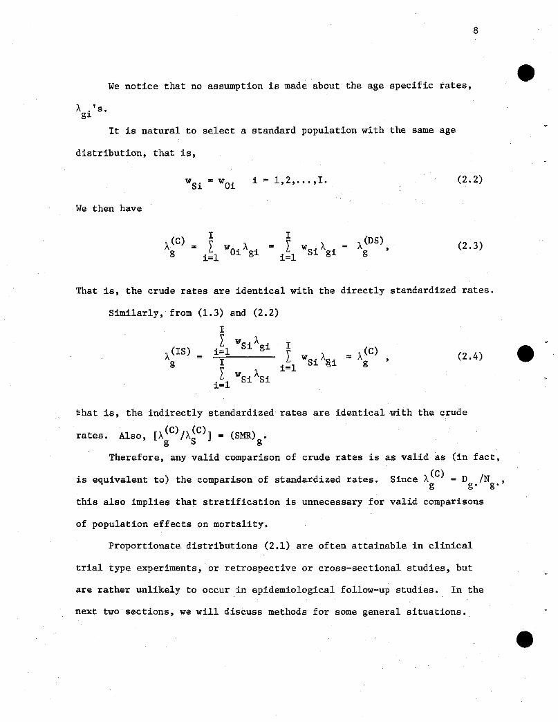
We notice that no assumption is made about the age specific rates,

It is natural to select a standard population with the same age

distribution, that is,

i = 1,2,. .. ,1. (2.2)

We then have

A(C) =g

I

I wOo A i =i=l 1. g

II wS . A •

i=l 1. g1.A(DS)

g , (2.3)

That is, the crude rates are identical with the directly standardized rates.

(2.4)= A(C)g

I

I WS · A~.i=l 1. ~1.I

I wSi AS·i=l .1.

A(IS) =g

Similarly, from (1.3) and (2.2)

II WSi Agii=l

rates.

~hat is, the indirectly standardized rates are identical with the crude

Also [A(C)/A(C)] = (SMR) •, g S g

Therefore, any valid comparison of crude rates is as valid as (in fact,

is equivalent to) the comparison of standardized rates. Since A(C) = D INg g. g"

this also implies that stratification is unnecessary for valid comparisons

of population effects on mortality.

Proportionate distributions (2.1) are often attainable in clinical

trial type experiments, or retrospective or cross-sectional studies, but

are rather unlikely to occur in epidemiological follow-up studies. In the

next two sections, we will discuss methods for some general situations.

9

3. 'EXTERNAL STANDARDIZATION: HOW TO "TEST" FOR ITS VALIDITY

3.1. Consider G study populations and an external (standard),population

(S), stratified into I age strata. We wish to compare mortality patterns

in the study populations with that of the standard population using

standardized rates (external standardization).

Assume first that multiplicative models for age specific rates of

the form

Model M: A. = 0 E., g = 1,2, ... ,G,g g1 g 1 (3.la)

(3 .lb)

for i = 1,2, ..., I, hold • Here the E. 's represent the main stratum1

effects, and the 0 's represent the main population effects; there is nog

'interaction' term, 68i

, say (in statistical terminology, no ~nteraction'

on a logarithmic scale) among the populations and age strata.

Under (3.1), the expected number of all deaths in the gth population

is

I,E(D 1M) E(D ) L N .0 Ei 0 -= = = N Eg. g g.

i=l gl. g g- g g

where

-1I- LN. E.E = Ng g. i=l gl. l.

and similarly,

E(DS.IMs) = E(DS '> = NS.OS£S

(3.2)

(3.3)

(3.4)

10

3.2. Indirect ~tandardization. We wish to compare death rates in

each study population with the corresponding rates in the standard population.

Formally, for the gth population, we wish to test the null nypothesis

or equivalently ,(if lllodel (3.1) 'is- va1i.d},

H(g) • 0 ~o • g = Us '

against the alternative

(3.5)

(3.6)

H(g)·A . (3.?)

In other words, we wish to fit model MS of the standard population

to each study population separately.

If H(g) is true we have,o

(3.8)

so that

If, however, Hcig) is not true,

E(D )/E(D IHO(g» = 0 los = y ,say.g. g. g g

Comparing (3.8) and (1.4), we notice that under model (3.1),

(3.9)

(3.10)

(3.11)

11

gives the expected number of deaths under indirect standardization. This

also implies that (3.10) is approximately the expectation of the standardized

mortality ratio, that is

(3.12)

Thus, assuming model (3.1) is valtd~ the SMR's measure the relative

(with respect to a standard population) mortality effects of the study

populations.

We also have

(3.13)

3.3. Direct standardization. In indirect standardization, the

mortality rates of the standard population are used as; a.-.odel f-or:;eacht of thed

study populations. In direct standardization, we say that the same weights,

wSi's, are used in calculating an average rate for each study population.

But this can also be interpreted in a different way. The standard population

can be considered as an experimental population toWhich we try to fit dif-

H(Sg)o . , say,ferent models (study populations). We now test a null hypothesis,

(Sg)that .the·popuIati~nGS)~~;tt$.a... mOdel.Mg' that is, HO : ASi = Agi = <5 E.g 1.

for all i.

Formally, we also have

E(D jH(Sg» =S· 0

so that

II Ns ·<5 E. = NS· . <5 gEsi=l 1. g 1.

(3.14)

E(D !H(Sg»/E(D ) =s. 0 s· (3.15)

12

which is the same as (3.10). (Note, however, the differences in the structure

and meanings of (3.10) and (3.15).) Also,

(3.16)

which is identical with (3.13).

Thus, when model (3.1) is valid, the expected values of indirect and

direct standardized rates are the same. This implies that effectively, either

kind of standardization leads to the same result. There is, however, some

difference in interpretation. With indirect standardization we fit the

data (i.e., each study population) to the model (standard population); with

direct standardization, the model is fitted to the data, which is not quite

what we should do. For this reason, I would prefer indirect standardization. ~

Freeman and Holford (1980) favored directly standardized rates, because they

also give valid comparisons under additive. model (1.8).

3 ..4. "Testing" for multiplicative model (3.1). The results presented

above are based on the assumption that the multiplicative model (3.1) holds.

How do we know that this assumption is correct, so that the standardized

indices would give valid comparisons?

This may be known from past experience or, perhaps, obtained from the

data. Since we are dealing with finite populations of known sizes, we can

treat them as samples from infinite populations. Formally, we then can

construct some tests of goodness of fit, but since the populations are

very large, any test will nearly always give highly significant results.

Therefore, we may use some other indicators which would suggest that model

(3.1) is acceptable.

13

(i) A simple, but very useful method of assessment of (3.1) is to calculate

ratios, Ag/ASi ' i = 1,2, ••• ,1. If these ratios are fairly consta;nt over

all strata in each population, but may differ from population to population,

then this would be an indicator that a multiplicative model is applicable.

Often it holds approximately over a restricted age range, for example, 30-75.

(c.f. Table lB). In such cases, we may confine our analysis to this age

range.

(ii) It was mentioned in Section 3.3, that if model (3.1) holds,

the directly and indirectly standardized rates should be approximately equal

in each population. This would provide another check, but should be used

in conjunction with the method described in (i); close values of direct and

indirect standardized rates can be obtained even if (3.1) does not hold

e (see Table lD).

3.5. "Testing" for significance of population effects. We can cal-

culate some kind of formal Chi-square statistics. These, of course, will

be practically almost always statistically "significant" (yielding very

often huge values), but they may be used as relative measures of discrepancy ~.

as described below.

(i) Since the numbers of deaths, D . 's are rather small as comparedg~

to population sizes N . 's, it is reasonable to regard each D . as a Poissong~ . g~

variable, with mean, ~gi = NgiAgi , and conditional on Ngi's, the Dgi'S

are independent. Assuming model (3.1) is valid, and Hag): Og = Os is true,

the statistic

(3.17)

14

where Egi = NgiASi = NgiOSEi is defined in (1.4), is approximately distributed

as X2 with I degrees of freedom. Also, under H6g

) ,

X2~omb,g

(3.18)

is approximately distributed as X2 with 1 degree of freedom.

Finally,J2 = X2 _ X2-"TIif , g g 'Comb,g (3.19)

is approximately distributed as X2 with I-I degrees of freedom.

All these X2 ,s will usually be highly significant. We now introduce

a quantity

(3.20)

Assuming model (3.1) is correct, and

(a) If H(g): ° = ° is true, X2 should be rather small aso g S Comb,g2 2compared to X , so that we should have H relatively large (for large I, H +1).g g g

(b) If the alternative Hig>:%s=Yg is true, then X~Omb,g should be of the same

order of magnitude as X2, so that H2 should be relatively small (H2+O). Thus,g g g

H~ measures conformity with or departure from H6g) under th~ assumption that

(3.1) is correct. Some theoretical justification for (a) and (b) is given

in Appendix.

We should be aware, however, that if model (3.1) does not hold, i.e.

we observe 'interaction', then we have a similar situation as in (a), but

H~ measures departure from model (3.1) rather than conformity with H6g)·

Therefore, it is advisable to check first the adequacy of model (3.1).

(ii) Finally, we may fit multiplicative model (3.1) to all data

including (or excluding) the standard population. Let 6g and ~i be the

15

no longer represents a Chi-square statistic.

corresponding estimates of 0g

A A

value of D . is then N iO E ••g1 g g 1

and E., respectively. The estimated expected1

I A A 2Now, the quantity, L (D i-N i O E.) IN .8 ~i

i=l g g g 1 g1 g

It is a contribution to the

overall Chi-square,

2XTotal =

G I A A 2 A A

L L [(D i-N .0 Ei ) IN .0 E.]g=l i=l g g1 g g1 g 1

(3.21)

If model (3.1) is correct, (3.21) is approximately distributed as

X2 with (G-l)(I-l) degrees of freedom.

Similarly, X2 is only a contribution toComb,g

(3.22)=GL (D -E )2 /E

g=l g. g' g.

Nevertheless, the indices, H2,s are still useful checking for conformityg

with multiplicative model (3.1), considered jointly with indicators discussed

in Section 3.4. (More details on fitting multiplicative models are given

in Section 4.)

EXAMPLE 1. The data in Table lA represent the U.S. white male pop-

ulations and counts of death from Ischemic Heart Disease (IHD); as defined

in ICDA, Eighth Revision by code numbers 410-413, over the period 1968. The

data are from U.S. Vital Statistics, Part IIA,1968-l977. It is claimed

(in: . Proceedings (1979)} that there is a definite declining

trend in mortality from IHD; the directly standardized rates using U.S.

White Male, 1940 population as standard were used in this monograph. We now

apply the methods discussed in this paper to search for this trend, and to

measure it, using external standardization.

TABLE lAU.S. WHITE MN,ES - ISCHEMIC HEART DISEASE; (410-413) OVER PERIOD 1908-1977

1968 1969 1970 (Census) 1971 1972Age N '10- 3 DU

N .10-3 -3 D4i-3

(i) Group 11 2i D2i N3i D3i N4i·10 N5i '10 D51

1 0-1 1,444 17 1,471 10 1,501,250 7 1,543 16 1,412 42 1-5 6,434 7 6,139 3 5,873,083 3 5,851 5 5,889 63 5-10 9,049 7 8,988 6 8,633,093 7 8,339 7 8,058 44 10-15 8,839 3 8,954 6 9,033,725 6 9,140 14 9,103 85 15-20 7,906 23 8,037 27 8,291,270 21 8,551 43 8,727 226 20-25 6,367 55 6,671 71 6,940,820 32 7,572 74 7,650 747 25-30 5,536 188 5,740 190 5,849,792 223 6,051 213 6,588 212

SUM 45,575 300 46,000 313 46,123,033 349 47,047 372 47,427 330

8 30-35 4,789 655 4,876 650 4,925,069 656 5,097 701 5,295 6349 35-40 4,910 2,386 4,822 2,333 4,784,375 2,203 4,761 2,175 4,777 1,980

10 40-45 5,333 6,572 5,270 6,300 5,194,497 6,006 5,139 5,876 5,071 5,65211 45-50 5,235 13,259 5,297 13,043 5,257,619 12,629 5,256 12,398 5,205 12,19212 50-55 4,747 21,495 4,799 21,182 4,832,555 20,924 .4,946 20,868 5,061 20,94413 55-60 4,224 31,913 4,297 31,471 4,310,921 31,134 4,370 30,945 4,393 30,16214 60-65 3,494 41,691 3,551 41,170 3,647,243 40,874 3,728 40,998 3,788 42,05215 65-70 2,761 48,244 2,817 47,854 2,807,974 47,694 2.891 47,544 2,971 48,49416 70-75 2,047 54,860 2,043 53,362 2,107,552 52,029 2,116 51.411 2,117 52,006

SUM 37,540 221,075 37,772 217,365 37,867,805 214,149 38,304 212,916 38,678 214,116

17 75-80 1.472 54.878 1,471 53,677 1,437,628 53,000 1,458 53,399 1,453 54,01418 80-85 824 43,828 842 44,258 805,564 43,794 826 44,149 845 44,85419 85+ 414 38,299 429 39,189 486,957 39,756 465 41,982 477 42.222

SUM 2,710 137,005 2,742 137,124 2,730,149 136,550 2,749 139,530 2,775 141,090

Total 85,825 358,380 86.514 354,802 86,720,987 351,048 88.100 352,818 88,880 355,536

TABLE 1A (Continued)

1973 1974 1975 1976 1977 TotalAge -3 -3 -3 -3 -3

(i) Group N6i ·10 D61 N7i

.10 D7i

N8i'10 D8i N9i '10 D9i N10i

'10 D10i No! D' i

1 0-1 1,318 12 1,286 6 1,312 7 1,293 5 1,345 9 13,925,250 932 1-5 5,836 1 5,668 1 5,417 5 5,189 5 5,079 1 57.375,083 343 5-10 7,774 5 7,531 1 7,401 2 7,397 2 7.293 4 80.1+63,093 454 10-15 9,032 10 8,950 7 8,780 5 8,491 5 8,200 4 88,522,725 685 15';'20 8,868 34 8,971 27 9,029 22 9.107 17 9,059 24 86,546,270 2606 20-25 7,803 71 7,990 64 8,219 69 8,390 55 8,557 52 76,159,820 6677 25-30 6,793 202 7,068 178 7,366 207 7,729 220 7,652 183 66,372,792 2,016

SUM 47,424 335 47,464 284 47,524 317 47,596 306 47,185 277 469,365,033 3,183

8 30-35 5,532 659 5,856 663 6,044 641 6,161 656 6,7.02 679 55,377,069 6.5949 35-40 4,831 1,974 4,906 1,829 4,973 1,779 5,098 1,732 5,282 1,750 49,144,375 20,141

10 40-45 4,988 5,430 4,907 4,988 4,820 4,775 4,795 4,634 4,803 4,284 50,320,497 54,51711 45-50 5,180 11,864 5,129 11,380 5,095 10,463 5,042 10,050 4,971 9,360 51,667,619 116,63812 50-55 5,130 20,397 5,178 19,723 5,180 19,105 5,165 18,116 5,114 17,557 50,152,555 200,31113 55-60 4,419 30,594 4,466 28,658 4,553 27,703 4,643 27,030 4,759 26,367 44,434,921 295,97714 60-65 3,835 40,971 3,883 39,299 3,907 38,195 3,952 37,625 3,979 36,115 37,764,243 398,990 I-'15 65-70 3,049 48,357 3,127 47,486 3,220 46,409 3,279 45,991 3,342 45,115 30,264,974 473,188 '"16 70-75 2,152 51;444 2,193 50,144 2,226 48,521 2,284 48,458 2,365 48,641 21,650,552 510,876

SUM 39,216 211,690 39,645 204,170 40,018 197,591 40,419 194,292 41;317 189,868 390,776,805 2,077,232

17 75-80 1,428 52,363 1,419 49,429 1,435 47,689 1,442 47,687 1,448 46,8(}2 14,463,628 512,93818 80-85 865 45,819 870 43,717 874 42,468 892 42,623 897 42,039 8,540,564 437,54919 85+ 493 43,979 520 44,342 549 43,052 561 44,624 583 44,794 4,977,957 422,239

SUM 2,786 142,161 2,809 137,488 2,858 133,209 2,895 134,934 2,928 133,635 27,982,149 1,372,726

_Tote 89,426 354,186 90,118 341,942 90,400 331'- 90,910 329,532 91,430 323,780 888,123,987 AJ,141--- .

- T:ttB -DEATH RATES AND THEIR RATlOS TO DEATH RATES OF STANDARD (EXTERNAL) POPULATION WM 1970 (CENSUS)

1968 1969 1970(CenGus) 1971 1972

Age ). .105 Y .102 ). .105 YZi·t02 ).3i .10 5 Y3i ·102 Y4i '10 5 ).4i· 102 y5i·105 ). .102

(i) Group Ii .Ii Zi 5i

1 0-1 1.18 252.49 0.68 . 145.79 0.47 .100 1.04 222.39 0.28 60.752 1-5 0.11 212.99 0.05 95.67 0.05 100 0.09 167.30 0.10 199.463 5-10 0.08 95.40 0.07 82.33 0.08 100 0.08 103.53 0.05 61.224 10-15 0.03 51.10 0.07 100.89 0.07 100 0.15 230.62 0.09 132.325 15-20 0.29 114.86 0.34 132.64 0.25 100 0.50 198.54 0.25 99.536 20-25 0.86 73.12 1.06 90.09 1.18 100 0.98 82.72 0.97 81.887 25-30 3.40 89.08 3;81 86.83 3.81 100 3.52 92.34 3.22 84.41

8 30-35 13.68 102.68 13.33 100.08 13.32 100 13.75 103.26 11.97 89.899 35-40 48.59 105.54 48.38 105.07 46.05 100 45.68 99.21 41.45 90.02

10 40-45 123.23 106.58 119.54 103.39 115.62 100 114.34 98.89 111.46 96.4011 45-50 253.27 105.44 246.23 102.51 240.20 100 235.88 98:20 234.24 97.5212 50-5~ 452.81 104.58 441.38 101.94 432.98 100 421.92 97.44 413.83 95.5813 55-60 755.52 104.61 732.39 101.41 722.21 100 708.12 98.05 686.59 95.0714 60-65 1193.22 106.47 1159.39 103.45 1120.68 100 1099.73 98.13 1110.14 99.0615 65-70 1747.34 102.87 1698.76 100.01 1098.62 100 1644.55 96.82 1632.25 96.1016 70-75 2680.02 108.56 2611.94 105.80 2468.69 100 2456.59 98.42 2456.59 99.51

17 75-80 3728.12 101.13 3649.01 98.98 3686.63 100 3662.48 99.35 3717.41 100.8418 80-85 5318.93 97.84 5256.29 96.69 5436.44 100 5344.92 98.32 5308.17 97.6419 85+ 9250.97 113.31 9134.97 111.89 8164.17 100 9028.89 110.59 8851.57 109.27

TABLE 1B (Continued)

1973 1974 1975 1976 1977 1968-77

(i) Age).6i·105 y 6i ·102 ).7i. 105 Y7i .102 ).8i· 105 Y8i· 102 ).9i· 105 Y .102

).10i· 105 ylOi

·102 lOi· 105Group 9i

1 0.,.,1 0.91 195.26 0.47 100.06 0.53 114.42 0.39 82.93 0.67 143.51 0.67.2 1-5 0.02 33.55 0.02 34.54 0.09 180.70 0.04 75.46 0.02 38.54 0.063 5-10 0.06 79.32 0.01 16.38 0.03 33.33 0.03 33.35 0.05 67.65 0.064 10-15 0.11 166.70 0.08 117.76 0.06 85.74 0.06 88.66 0.05 73.44 0.085 15-20 0.38 151.38 0.30 118.83 0.24 96.20 0.19 73.70 0.26 104.60 0.306 20-25 0.91 77.02 0.80 67.80 0.84 71.06 0.66 55.49 0.61 51.44 0.887 25-30 2.97 78.01 2.52 66.06 2.81 73.72 2.85 74.67 2.39 62.74 3.04

8 30-35 11.70 87.85 11.32 85.00 10.61 79.62 10.65 79.94 10.13 76.06 11.919 35-40 40.86 88.74 37.28 80.96 35.77 77.69 33.97 73.78 33.13 71.95 40.98

10 40-45 108.86 94.15 101.65 87.92 99.07 85.68 96.64 83.58 89.19 77.14 108.3411 45-50 229.03 95.35 221.88 92.37 205.36 85.49 199.33 82.98 188.29 78.39 225.7512 50-55 397.60 91.83 380.90 97.97 368.82 85.18 350.75 81.01 343.31 79.29 399.4013 55-60 692.33 95.86 641.69 88.85 608.46 84.25 582.17 80.61 554.04 76.71 666.09 f-'14 60-65 1068.34 95.33 1012.08 90.31 977 .60 87.23 952.05 94.95 907.64 80.99 1056.53

-.,J

15 65-70 1586.00 93.38 1518.58 89.41 1441.27 84.85 1402.59 82.58 1349.94 79.48 1563.4816 70-75 2390.52 96.83 2286.55 92.62 2179.74 88.30 2121.63 95.94 2056.70 83.31 2359.64

17 75-80 3666.88 99.46 3483.37 94.49 3323.28 90.14 3307.00 89.70 3232.18 87.67 3546.4018 80-85 5296.99 97.43 5024.94 92.43 4859.04 89.38 4778.36 87.90 4686.62 86.21 5123.1919 85+ 8920.69 109.27 8527.31 104.45 7841.89 96.05 7954.37 97.43 7683.36 94.11 8482.17

- e e

......00

standardization.

19

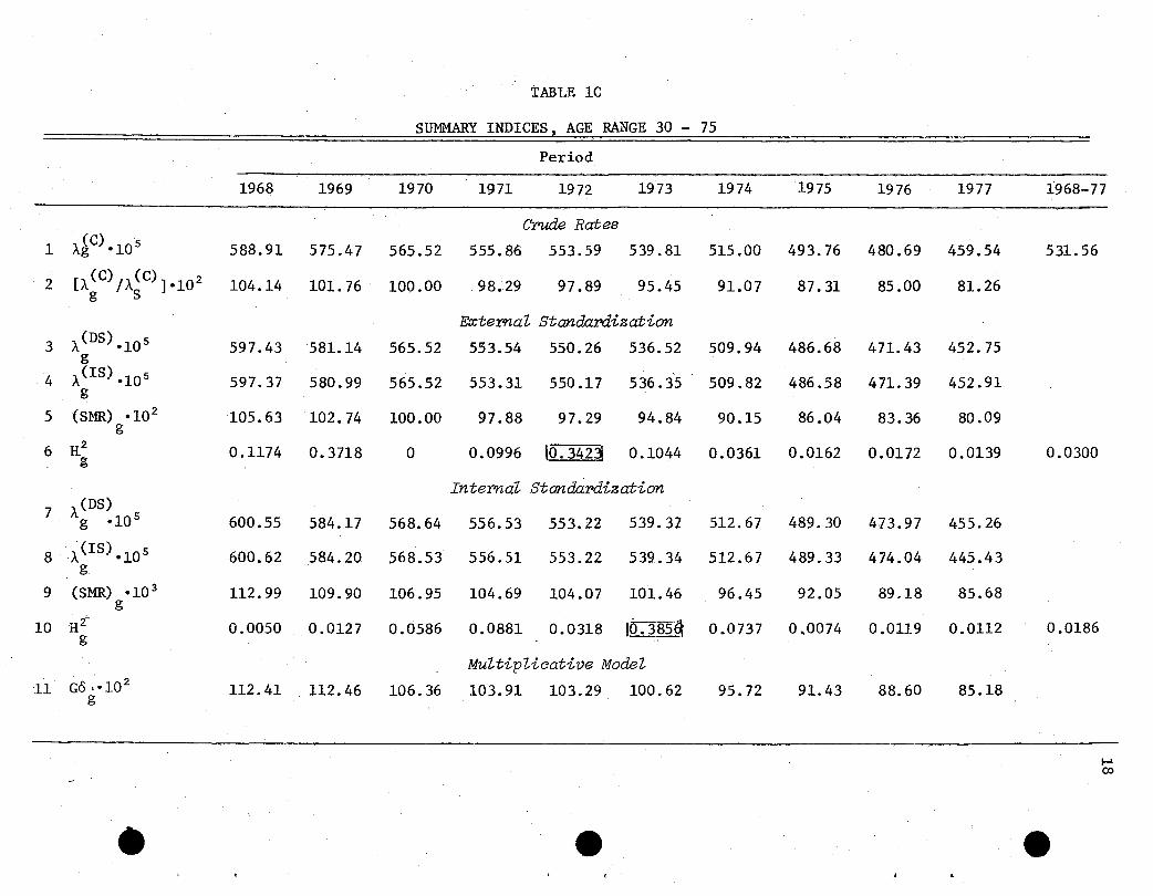
As a standard (S) population, we use here the U.S. white male,

1970 (Census) population. Table lB exhibits observed rates, Ai'105, and,g

2their ratios to the death rates of standard population multiplied by 10 ,

2Y '10 for g = 1,2, ••• ,G. These ratios seem to be more stable for adultg

ages, showing a rather excessive departure from stability for very young

ages and moderate departures for old ages. We decided first to analyze

mortality trends in the 30-75 age range; this is also the range which

is often used in epidemiological studies. The results are given in Table lC.

The rows 3-6 exhibit the indices discussed in this section for external

(Internal standardization, shown in rows 7-10, is discussed

in Section 5.J We assume that values of the H2 ,s of the order of magnitudeg

0.10 - 0.20 are sufficiently small, to reject the hypothesis H~g). Here,

~ population 5 (1972) seems to deviate from these limits. Generally, we can

reasonably assume that the data fit fairly well the multiplicative model (3.1).

To give some idea about the magnitudes of x2,s, we quote the results forg ,

populations 1, (1968), population 8 (1975), and total (1968-77).

x2:

g

x2 •Comb,g'

2XDif ,g:

H2g

1968 1975 (1968-77)

752.41 4548.54 24951.84

664.04 4474.76 24203.92

88.37 73.78 747.92

0.1174 JO.0162 0.0300

We also fitted the multiplicative model to the data, including the

standard 1970 (Census) by the maximum likelihood method, subject to theG

condition I Og =1. The results (for G = 10, and I = 9) are:g=l

e e e

21

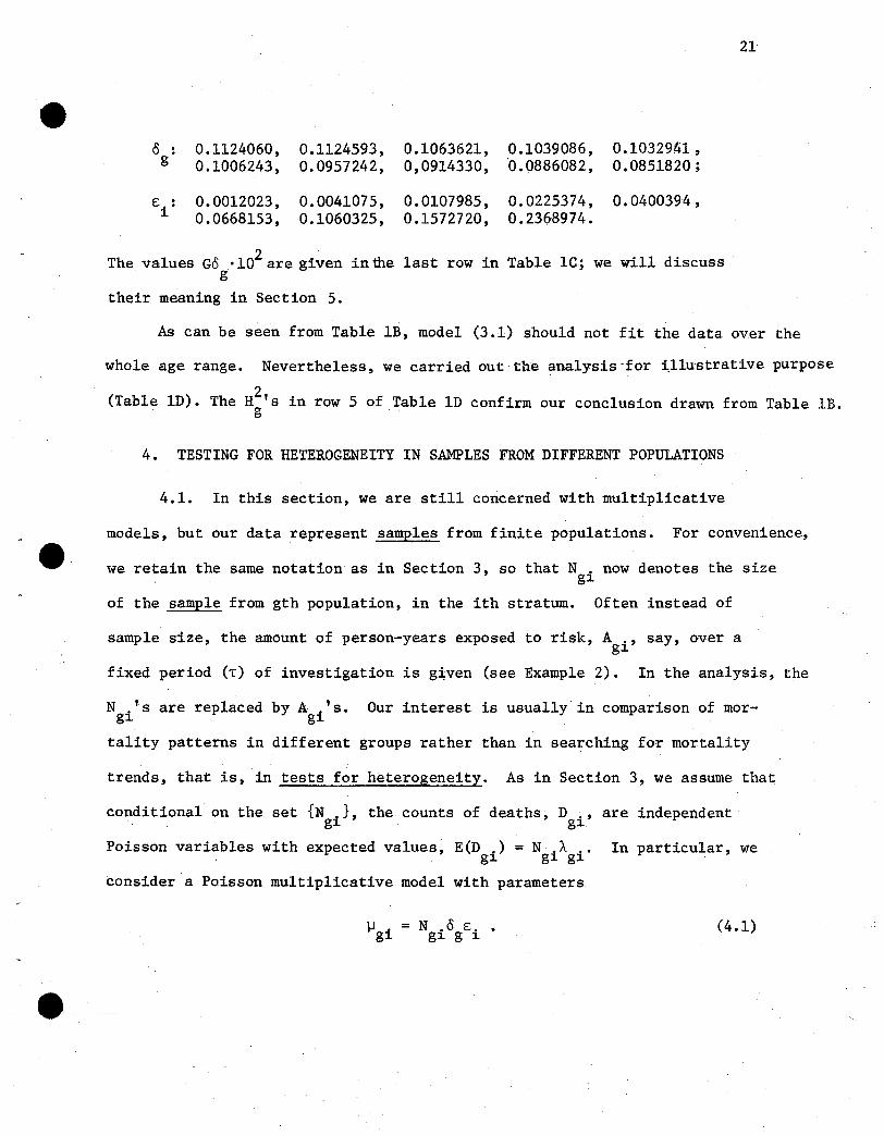
0 . 0.1124060, 0.1124593, 0.1063621, 0.1039086, 0.1032941,.g 0.1006243, 0.0957242, 0,0914330, ·0.0886082, 0.0851820 ;

E. : 0.0012023, 0.0041075, 0.0107985, 0.0225374, 0.0400394,~ 0.0668153, 0.1060325, 0.1572720, 0.2368974.

2The values Go ·10 are given in the last row in Table Ie; we will discussg

their meaning in Section 5.

As can be seen from Table lB, model (3.1) should not fit the data over the

whole age range. Nevertheless, we carried out the analysis -for i,llustrativepurpose

(Table lD). The H2,s in row 5 of ,Table lD confirm our conclusion drawn from Table lB.g

4. TESTING FOR HETEROGENEITY IN SAMPLES FROM DIFFERENT POPULATIONS

4.1. In this section, we are still concerned with multiplicative

models, but our data represent samples from finite populations. For convenience,

we retain the same notation as in Section 3, so that N . now denotes the sizeg~

of the sample from gth population, in the ith stratum. Often instead of

sample size, the amount of person-years exposed to risk, A ., say, over ag~

fixed period (T) of investigation is g~ven (see Example 2). In the analysis, the

N .'s are replaced by A i's. Our interest is usually in comparison of mor-g~ g

tality patterns in different groups rather than in searching for mortality

trends, that is, in tests for heterogeneity. As in Section 3, we assume that

conditional on the set {Ngi }, the counts of deaths, Dgi

, are independent

Poisson variables with expected values, E(D .) = N .J.. ., In particular, weg~ g~ g~

consider a Poisson multiplicative model with parameters

11 • = N .0 E ••g~ g~ g ~

(4.1)

22

Several authors (e.g. Osborn (1974), Breslow and Day (1975), Gail

(1978)) have discussed these models and their applications to various sets

of data. Theoretical bases for constructing various tests are elegantly

presented by Andersen (1977), and can be used for further reference for con-

structing various test statistics. We confine ourselves here to the Pearson-

2type X -tests.

4.2. The likelihood function leads to the set of GI likelihood

(4.2)

(4.3)

(4.4)

(Andersen (1977), Section 2). These equations can be solved using a computer

program.

2The Pearson-type X goodness of fit criterion is

(4.5)

A A

(cf. (3.21)). If the N iO E. 's are large enough (Le. ~ 10), (4.5) isg g ~

approximately distributed as X2 with (G-l)(I-l) degrees of freedom, )provided the

multiplicative Poisson model (4.1) is correct.

Of special interest is the null hypothesis, HO' that all 0g'S are the

1same, and in view of (4.4), HO: 0g = G for g = 1,2, ••• ,G. In this case,

23

equations (4.2) can be solved explicitly, yielding

AD .

.l.E. = G-1. N .•1.

(4.6)

Since the null hypothesis, HO' can also be expressed in the form

H • A = AOi for g = 1,2, ••• ,G" the ma:x:imum likelihood estimate of A01.' isO· gi

AD ••l.Ei = N:" '

.1.(4.7)

and the estimated expected value of D . under HO isgl.

E[D .IHo)]gl.t"

E ••g1.(4.8)

If HO is true, the statistic

is approximately distributed as X2with IG-I=I(G-l) degrees of freedom.

The quantity

2 A 2 A

Ygi = (D i-N .AOi) IN .AO'g g1. g1. 1.

(4.9)

(4.10)

2represents the contribution of the (gi)th cell to the X -statistic (4.9).

I 2Note that each sum LY . represents only a contribution of the gth sample

i=l gl.to the overall x2-statistic defined in (4.10), but is not itself distributed

4.3. It appears that D .'s are sufficient statistics for E.'S (see.1. l.

formula (4.6». Since the distribution of D.i's does not depend on 0g'S,

a multinomial distribution with

Poisson variates, Dgi , conditional on D. i have

index D i and parameters N . IN ., when HO

is• g1 ·1

24

they are also ancillary for 0 'so (Andersen (1977), Section 5). Therefore,g

inferences about 0 's can be derived from the distributions of theg

D its conditional on D .'s.g ·1

For the ith stratum, the

valid.

Note that

N . D . A~ ·1

D i-D. N = D .-N i -N-- = D .-N .AO·g ·1. i g1 g.i g1 g1 1

Therefore, under HO

' the statiatic

(4.11)

(4.12)

has, indeed, an. approximate X2 distribution with G-l degrees of freedom,

and

2 X2XTotal = =

I

Li=1

x~1 (4.13)

has a n approximate X2

identical with (4.9).

distribution with (G~l)I degrees of freedom; it is

Also,

where

2XComb =

G A 2L (D -E ) IEg=l g. g. g.

(4.14)

Eg.

I A

= L E. =i=l g1

I A I. DiINA =IN _.­

i=l gi Oi 11;;1, gi N. i(4.15)

is approximately distributed as X2 with G-l degrees of freedom. Also,

x2 = X2 _ X2 (-~if Total Comb 4.16)

is approximately distributed as X2

with (G....l) (1-1) degrees of freedom. It should

25

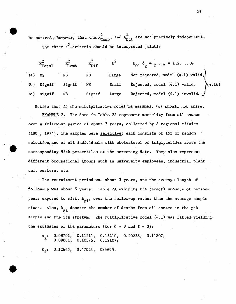
be noticed t how.ever t that the_X~omb and~if ,are not_ precisely independent.

The three X2-criteria should be interpreted jointly

2 X2 2 H2 HO

: 8 1 1,2, ••• ,GXTotal XDif

= - , g =Comb g G

(a) NS NS NS Large Not rejected, model (4.1) valid,

(b) Signif Signif NS Small Rejected, model (4.1) valid, (4.16)

(c) Signif NS Signif Large Rejected, model (4.1) invalid.

NotiCe that if tne multf.plicative model 'is assumed, . (c) should not arise.

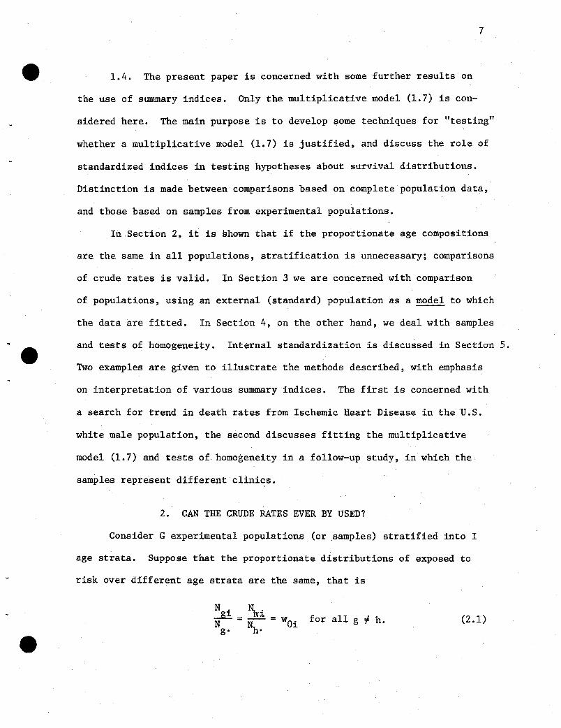
EXAMPLE 2. The data in Table 2A represent mortality from all causes

over a follow-up period of about 7 years, collected by 8 regional clinics

(LRCF, 1974). The samples were selective; each consists of 15% of random

selectio~and of all individuals with cholesterol or triglycerides above the

corresponding 95th percentiles at the screening date. They also represent

different occupational groups such as university employees, industrial plant

unit workers t etc.

The recruitment period was about 3 years, and the average length of

follow-up was about 5 years. Table 2A exhibits the (exact) amounts of person-

years exposed to risk, A ., over the follow-up rather than the average sampleg1.

sizes. Also, D i denotes the number. of deaths from all causes in the gthg .

sample and the ith stratum. The multiplicative model (4.1) was fitted yielding

the estimates of the parameters (for G = 8 and I = 3):

o.: 0.08701, 0.11511, 0.15410, 0.20228, 0.11807,g 0.09861, 0.10375, 0.12107;

e:. : 0.12645, 0.47024, 084695.1.

TABLE ZB

TESTING FOR HETEROGENEITY

CLINICS

Age 1 Z 3 4 .5 6 7 a Total

Group DEli

ZDZi EZi

Z 2 2 2 2 2 2X2 d.f. 2

(i) li Yli Y2i D31 E31 Y3i D41 E41 Y4i D5i E51 Y51 D61 E6i Y6i D71 E7i Y7i

Da1 E8i Y"81 1 X. 95

30-45 1 0.1+8 0.5633 2 1.81 0.0199 3 1.68 1.0371 0 1.27 1.2700 1 1.60 0.2250 1 2.47 0.8749 2 2.62 0.1467 6 4.08 0.9035 5.0404 7 14.07 NS

45-55 0 1.33 1.8300 1 2.26 0.0725 7 5.03 0.7716 3 1.59 1.2504 6 4.19 0.7819 6 6.22 0.0078 5 4.94 0.0007 5 6.95 0.5471 5.8920 7 14.07 NS

55-70._1_ 0.55 0.3682 2 1.21 0.5158 3 3.37 0.0406 3 0.64 18.70251 2 3.35 0.5440 3 3.53 0.0796 6 7.49 0.2964 6 5.87 0.0029 10.5500 7 14.07 NS-. - - - - - - - - - - - - - - - - - - - - - - - - - - - - - - - - - - - - - - - - - - - - - - - - - - - - - - - - - - - - - - - - - - - - - - - - - - - --SUM 2 2.86 2.7615 5 5.28 1.2382 13 10.08 1.8493 6 3.50111.22291 9 9.14 1.5509 10 12.22 0.9623 13 15.05 0.4438 17 16.90 1.4535 21.4824 21 32.67 NS

x2COmb

3.5902 7 14.07 NS

X2Dif 17.8922 14 23.67 NS

H2 0.8329--.,...,------------------'--------------------------------....:----'---------N

'"

e - e

27

4It The X2-statistic" calculated from (4. ) is equal to 15.04 with 14 d.f. and

is not significant (NS) at the significance level a = 0.05 (X 2• 95 ;14 = 23.67).

Next, we test the hypothesis, HO' that the 0g'S are all equal to

(l/G)= (1/8).A

The estimated expected values, E ., and the contributions tog~

X2 are given in Table 2B. We have the situation (4.l6(a» discussed above, so

the HO is not rejected. It seems that the non-sign1ficantresults are mainly

due to the smallness of the data set; in some classes there are only 1 or 0

deaths.

4.4. The tests of homogeneity discussed above can be formally applied

to population data. (For example, in studies of mortality patterns in different

countries.) However, if they are, the X2-values are usually highly significant,

and situations (4.l6(a)} and (4.16(c» might be sometimes indistinguishable.

geneity of type (4.l6(c» is detected, the populations might be arranged in

smaller subsets, for which either (4.l6(a» or (4.l6(b» holds. Alternatively,

we may try to get different models allowing for geographical effects, or

including interactions.

5 • INTERNAL STANDARDIZATION

5.1. We now return to Example 1 and assume that the multiplicative

model (3.1) is valid

range 30-75.

(including the 1970 census population), for age

With external standardization, we compared the effect (0 ) of eachg

study population with the effect (os) of the standard. We may also

wish to compare" the ° 's with an average effect of all populations,g

28

that is, when the standard population is composed of all study populations,

and the expected number of deaths in the gth population and ith stratum is

calculated from the formula

(5.1)

where D.i/N.i = AOi is the corresponding age specific rate in the combined

population. This is called internal standardization. Here,however, we

encounter some difficulty. If the multiplicative model M given by (3.1a)g

is valid, then in the general case, the model MS given by (3.1b) is now not

valid, so that Mg

and MS are inconsistent. To see this from (4.2), we have

where

Hence

and

_ -1 G0i = N. LN ·i·o~

.~ g=l g ....

(5.2)

(5.3)

(5.4)

-= N .e:.oig~ ~

(5.5)

Now the effect for the standard population, 6i , depends on i (the stratum), so

that (5.4) is not a multiplicative model.

5.2. Suppose that the study population distributions are proportional

(Section 2). In this case, we also have

Ngi = aOg ' saYJ for all i,N' i

Gwith I ao = 1,so that

g=l g

GI ao 0 = 6, for all i

g=l g g

Under these conditions, we have

29

(5.6)

(5.7)

We also have

E(D IHO) = Eg. g.(5.8)

so that

E(D )g.

I=6IN.E.,

i=l g3. 3.(5.9)

E(SMR) ::: E(D )/E(D .IHO) = 0 /6g. g' g. g (5.10)

Now, (SMR) measures the relative effect of the gth population withg

respect to the average effect of all study populations.

5.3. As already mentioned, 'perfect' proportionate distributions of study

populations are seldom encountered even in studies of the same population

over a certain period of years as can be seen in Example 1. Tables of wOi's

and aOg's (not given in this text) reveal such departures from proportionate

distributions. But in studies of the same population over a fairly short

period (e.g. ~ 10 years) these departures are quite commonly not so great that

they make a substantial difference to our results. The ratios A(C) /A (C)g S'

30

compared with the values of (SMR)g in row 5, do not differ considerably,

indicating that the assumption of proportionate distribution can be used

approximately. We have also computed a table of Agi!AOi ' analogous to Table lB

(not given in this text), which suggests that the combined population may be

reasonably used as a standard. Results of internal standardization are given

in rows 7-10 of Table lC. Except for population 6 (1973), the H2,s areg

smaller than for external standardization, indicating a fairly good fit of

multiplicative model, and reasonably small effect of the proportionality among

distributions.

A final check for the multiplicative model is given in the last row (11)

of Table lC. We notice that for the mult~plicativemodel

E(SMR) ~ E(D )!E(D IHo) = 0 ! Gl = Gog g. g. g g. (5.11)

If internal standardization is approximately valid, (5.11) given in row 11 of

Table lC should not deviate too much from the observed (SMR) given in row 9g

of Table lC. Except for population 2 (1969) the fit is rather good.

Surprisingly good agreement of row 9 and 11 in Table lD is also observed, though

not all ;::the l. :data seem to "fit. the Dlultiplica.t:i:ve model. Probably these

indices are sufficiently robust,that is, are not too sensitive to assumptions.

6. DISCUSSION

6.1. Though standardized rates have been widely criticized, they are

still used in epidemiological research. The criticism, however, did not relate

to an essential feature that these indices can be regarded as playing the role

of "statistics" in statistical inference. Thus, their appropriateness depends

on the underlying model for age specific rates as was recently emphasized by

Freeman and Holford (1980).

•

31

Suppose, for example, that we compare two means of a given characteristic,

using t-test (which is a kind of "index"). If the assumption that these means

are from normal populations does not hold, t-test is invalid. The same applies

to these indices: they are valid, for example, if a multiplicative model,

Agi = 0g8i (and ASi = 0S8i ) is valid,. or equivalently> when . \/A8i = %s.

6.2. The simplest way to analyze the data would be to fit the data to

the model (usually by the maximum likelihood method), and "test ll for its

appropriateness, using the H2-index :4n conjUmctionW±ththet:atioS,Ag/~i'

Which should be approximately constant 'f~r any' g;&h, if model Mg

is val·id. In case

of good fit. the GO's "C(5.ll"reveal the effects of differenj: P9pulations.• g'" 11 _

6.3. More traditionally, we may calculate standardized rates. As pointed

out in the text indirect standardization, especially (SMR) g 1.,$ pre(erab·le •.

6.4. If the proportionate distributions of study populations are

approximately the same, crude rates are identical to external (directly and

indirectly) standardized rates. Internal standardization can be used to evaluate

population effect as compared to the average effect of all study populations.

6.5. It seems that the standardized rates are 'robust estimators,' in

that they are not sensitve to assumptions required for their validity.

6.6. Multiplicative models appear to be appropriate for different types

(not necessary mortality) data, and are convenient mathematically. It would

be of some interest to perform similar analyses for additive models, A . = ¢ + a.,g1 g 1

and check for their validity for standardization.

Acknowledgement

I would like to thank Mr. G. Samsa for computing summary indices, and

Dr. N.J. Johnson for obtaining the maximum likelihood estimates.

32

REFERENCES

1. Andersen, E.B. (191,7). Multiplicative Poisson models with unequalcell rates. Second J. Statist. 4, 153-158.

2. Breslow, N. and Day, N.E. (1975). Indirect standardization and multi­plicative models for rates with reference to the age adjustment ofcancer incidence and relative frequency data. J. Chron. Dis. ~~,

289-303.

3. Doll, R. and Peto, E. (1981). The causes of cancer: quantitative estimatesof avoidable risks of cancer in the United States today. J. Nat.Cancer Inst. 66, 1193-1308.

4. Freeman, D.H. and Holford, T.R. (1980). Summary rates. Biometrics 36,195-205.

5. Gail. M. (1978). The analysis of heterogeneity for indirect standard­ized mortality ratios. J. Roy. Statist. Soc. Ser. A, ~~~, 224-234.

6. Internat~onal Classification of Diseases Adapted (ICDA) for use in theUnited States, Eighth Revision. U.S. DHEW, Public Health ServicePublication No. 1693, 1968.

7. Kitagawa, E.M. (1964). Standardized comparisons in population research.Demography ~, 296-315.

8. Kitaga~a, E.M. (1966). Theoretical considerations in the selection ofa mortality index and some empirical comparisons. Human Biology 38,293-308.

9. Lipids Research Clinics Program (LRCP) (1974). Protocol of the LipidResearch Clinics Prevalence Study. Central Patient Registry andCoordinating Center, Dept. of Biostatistics, University of NorthCarolina at Chapel Hill.

10. Osborn, J. (1975). A multiplicative model for the analysis of vitalstatistics rates. App1. Statistics :~, 75-84.

11. Proceedings of the conference on the Decline in Coronoary Heart DiseaseMortality (Eds. Havlik, R.J. and Feinlieb, M.) U. S. DEHW, PublicHealth Service, NIH Publication No. 79-1610, 1979.

12. Spiegelman, M. and Marks, H.H. (1966). Empirical testing of standardsfor the age adjustment of death rates by direct method. Human Biology38, 280-292.

13. Vital Statistics of the United States, 1968-17. Vol. II. MOrtality. PartA. DHEW Publications, 1972-1982.

14. Yerushalmy, J. (1951). A mortality index for use in place of the age adjusteddeath rate. f\m~_-!:..1.~~. Hea!!.l:!. il' 907-922. e

..

33

APPENDIX

Expected Values of "X2-Statistics" Under Different Hypotheses

We assume that the D .'s and DS"S are approximately Poisson variatesg~ .. ~

which have multiplicative models with expected values, ].lSi = Ngi(\Si and

~Si = NSiOSSi ' respective1y,and conditionally on sets {Ngi , NSi} they are

mutually independent.

Consider the null hypothesis H6g): Og/oS = 1, and the alternative

HA(g): °los = y .g g

We then have

E(D IH(g» = Var(D . IH(g)= Nos = E .gi 0 g~ 0 gi S i g~

e and

E(D .IH(g» =Var(D IH(g» = y Eg~ A gi A g gi

Similarly,

(A.1)

(A.2)

I

= LE . = Ei=l g~ g'

(A.3)

and

E(D /H(g» = Var(D IH(g» - y Eg. A g. A g g'

We now evaluate

(A.4)

= --!.-. [Var (Dg-t IHA(g» + (y -1) 2E~.]E • ... g g~g~

(A.5)

Thus

I (D -E )2E(X2 IH(g» = E ~ . gi gi IH(g) =

g . A .L1

E i A~= g

2Iy +(y -1) Eg g g.

34

(A.6)

Similarly,

so that

(D -E )2E(X2 IH(g» = E[ g. g' IHA(g)] = ~ +(y _1)2E (A.7)

Comb,g A Egg g.g.

Hence

(A.B)

(y _1)2E +Y= 1 - g. g. g + 1-1 = 0

(y -1)2E +y ,g g' g

(A.9)

•