Embed Size (px)
Citation preview

MomentumStephen Satchell, Yang Gao
Northfield Asia Research Seminar, 8th November, 2017
Stephen Satchell
University of Sydney Business School Trinity College, University of Cambridge [email protected]
Yang Gao
University of Sydney Business School [email protected]

Overview
1. General Thoughts
2. Partial Moment Momentum
3. Distribution of Momentum Returns
2

Topic 1: General Thoughts
Prensented by: Stephen Satchell
3

Momentum trading strategy
Cross sectional momentum (CSM) strategies are
employed by buying previous winners and selling
previous losers.
• Formation period, stocks are sorted based on
their past performances.
• Holding period, long winners (best performing)
while short losers (worst performing).
• Lag between formation and holding periods.
Doing so can avoid short-term reversals.
4

Profitability of momentum
Momentum is profitable if:
1. Strong deterministic trend.
2. Some autocorrelation.
3. High risk positions sometimes have
higher returns.
4. Reason 3 compatible with market
efficiency.
5
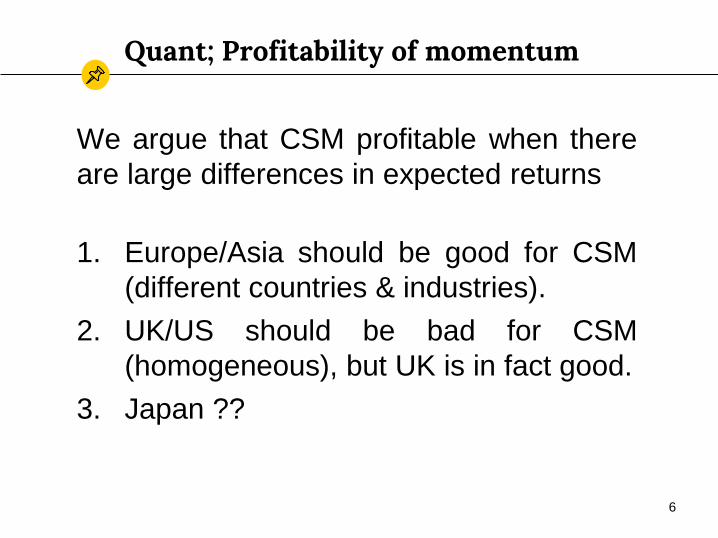
Quant; Profitability of momentum
We argue that CSM profitable when there
are large differences in expected returns
1. Europe/Asia should be good for CSM
(different countries & industries).
2. UK/US should be bad for CSM
(homogeneous), but UK is in fact good.
3. Japan ??
6

BF/Psychology; Profitability
1. Practitioners of BF would say implicitly,
Europeans, Brits, and Asians would
have persistent psychological problems
that do not correct.
2. Americans do not have these problems.
Quant explanation seems more plausible.
7
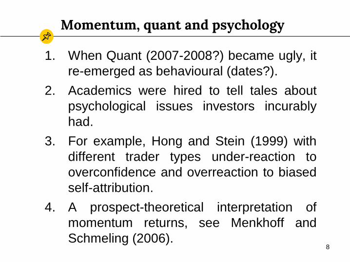
Momentum, quant and psychology
1. When Quant (2007-2008?) became ugly, it
re-emerged as behavioural (dates?).
2. Academics were hired to tell tales about
psychological issues investors incurably
had.
3. For example, Hong and Stein (1999) with
different trader types under-reaction to
overconfidence and overreaction to biased
self-attribution.
4. A prospect-theoretical interpretation of
momentum returns, see Menkhoff and
Schmeling (2006).8

Topic 2
Partial Moment Momentum
Yang Gao a, Henry Leung a, and Stephen Satchell a,b
Prensented by: Yang Gao
a University of Sydney Business School b Trinity College, University of Cambridge
9

Why volatility matters
• Momentum profits benefit from persistent
trends of the market which can be predicted
by market volatility.
Barroso and Santa-Clara (2015) and Daniel and
Moskowitz (2016) present evidence that scaling the
weights of momentum portfolios increases the
Sharpe ratio of the plain momentum strategy
10
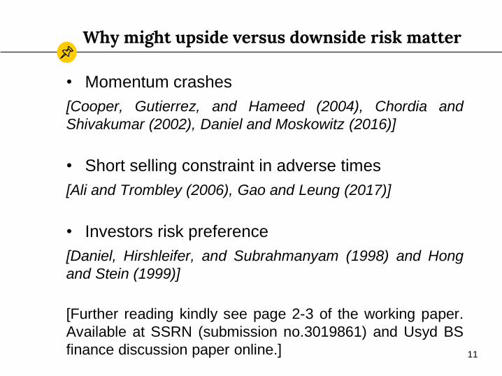
Why might upside versus downside risk matter
• Momentum crashes
[Cooper, Gutierrez, and Hameed (2004), Chordia and
Shivakumar (2002), Daniel and Moskowitz (2016)]
• Short selling constraint in adverse times
[Ali and Trombley (2006), Gao and Leung (2017)]
• Investors risk preference
[Daniel, Hirshleifer, and Subrahmanyam (1998) and Hong
and Stein (1999)]
[Further reading kindly see page 2-3 of the working paper.
Available at SSRN (submission no.3019861) and Usyd BS
finance discussion paper online.] 11
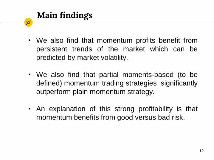
Main findings
• We also find that momentum profits benefit from
persistent trends of the market which can be
predicted by market volatility.
• We also find that partial moments-based (to be
defined) momentum trading strategies significantly
outperform plain momentum strategy.
• An explanation of this strong profitability is that
momentum benefits from good versus bad risk.
12
Data
• Monthly and daily US equity data over Jan 1927 to
Dec 2016 sourced from the CRSP via WRDS. Our
sample includes common stocks (CRSP share code
10 or 11) of all firms listed on NYSE, Amex and
Nasdaq (CRSP exchange code 1, 2 or 3).
• We use the value-weighted index of all listed firms
in the CRSP and 1-month Treasury bill rate as the
proxy for the market portfolio and the risk-free rate,
respectively. (Sourced from the Kenneth R. French
Data Library)
13

Partial moments
• Following the literature: Andersen, Bollerslev, Diebold & Ebens (2001),
Barndorff-Nielson (2002) and Baruník, Kočenda & Vácha (2016)
• We define monthly realised variance 𝑅𝑉 as
𝑅𝑉𝑡 =
𝑖=1
𝑛
𝑟𝑖,𝑡2
• We define lower partial moment 𝑅𝑃𝑀− and higher partial moment 𝑅𝑃𝑀+
as
𝑅𝑃𝑀𝑡− =
𝑖=1
𝑛
𝑟𝑖,𝑡2 𝐼 𝑟𝑖,𝑡 < 0
𝑅𝑃𝑀𝑡+ =
𝑖=1
𝑛
𝑟𝑖,𝑡2 𝐼 𝑟𝑖,𝑡 ≥ 0
• There is an identity𝑅𝑉𝑡 = 𝑅𝑃𝑀𝑡
− + 𝑅𝑃𝑀𝑡+
14
Estimation
1. We use daily data for our different volatility estimators
and use last month as our forecast for next month.
2. Alternatively, we also use a VAR(1) model based on
𝑅𝑃𝑀+and 𝑅𝑃𝑀−.
3. Method 2 does not do as well as method 1; old result
hard to beat a random walk out of sample one period
ahead.
15

Adapted Sortino ratio (an improvement on Sharpe ratio)
• a performance measure better capturing the downside risk
• We define monthly realised variance 𝑅𝑉 as
𝐴𝑑𝑎𝑝𝑡𝑒𝑑 𝑆𝑜𝑟𝑡𝑖𝑛𝑜 𝑟𝑎𝑡𝑖𝑜 =𝐸𝑥𝑐𝑒𝑠𝑠 𝑅𝑒𝑡𝑢𝑟𝑛
2 ∗ 𝐷𝑜𝑤𝑛𝑠𝑖𝑑𝑒 𝑆𝑒𝑚𝑖𝐷𝑒𝑣𝑖𝑎𝑡𝑖𝑜𝑛
where
𝐸𝑥𝑐𝑒𝑠𝑠 𝑅𝑒𝑡𝑢𝑟𝑛𝑡 = 𝑅𝑡 − 𝐷𝑒𝑠𝑖𝑟𝑒𝑑 𝑇𝑎𝑟𝑔𝑒𝑡 𝑅𝑒𝑡𝑢𝑟𝑛𝑡
𝐷𝑜𝑤𝑛𝑠𝑖𝑑𝑒 𝑆𝑒𝑚𝑖𝐷𝑒𝑣𝑖𝑎𝑡𝑖𝑜𝑛
=σ𝑖=1𝑁 (𝐸𝑥𝑐𝑒𝑠𝑠 𝑅𝑒𝑡𝑢𝑟𝑛𝑖−𝐸𝑥𝑐𝑒𝑠𝑠 𝑅𝑒𝑡𝑢𝑟𝑛)
2
𝑁𝐼 𝐸𝑥𝑐𝑒𝑠𝑠 𝑅𝑒𝑡𝑢𝑟𝑛𝑖 < 0
• Our adaptation differs from the standard Sortino (1994) ratio with
target return equal to the riskless rate, as, in the event that mean
returns are zero and 𝑅𝑃𝑀− = 𝑅𝑃𝑀+, we recover the Sharpe ratio. 16

PM-based momentum strategies
These have the potential to better capture market trends and hopefully avoid huge
losses during market rebounds using market decomposed variances.
1. Partial moment momentum strategy (PMM)
• Switching positions of the winner and loser portfolios during
the holding periods depending upon current estimates of
partial moments. (𝑅𝑃𝑀− & 𝑅𝑃𝑀+)
2. Extended partial moment-decomposed momentum
strategy (PMD)
• Scaling the weights of winner and loser portfolios towards
favourable/unfavourable volatility signals and holding an off-
setting position in cash.
17

Method 1, PMM construction
18
Two sets of CVs used for𝑅𝑃𝑀𝑡
+ and 𝑅𝑃𝑀𝑡−
1. 10th percentile of𝑅𝑃𝑀𝑡
+ and 75thpercentile of 𝑅𝑃𝑀𝑡
−.
2. Medians of 𝑅𝑃𝑀𝑡+
and 𝑅𝑃𝑀𝑡− .

PMM strategy analysis
In any given month t, conditions are classified based on partial moments in the previous month t-1 due to one-
month gap between the formation and holding periods; 𝒓𝒘,𝒕+𝟏,𝒓𝒍,𝒕+𝟏,𝒓𝒇,𝒕+𝟏 represent returns of winners, losers
and the risk-free asset in month t+1, respectively. Correspondingly, returns of momentum and contrarian
strategies are 𝒓𝒘,𝒕+𝟏- 𝒓𝒍,𝒕+𝟏 and 𝒓𝒍,𝒕+𝟏- 𝒓𝒘,𝒕+𝟏, respectively.
PMM Strategies Condition 1 Condition 2 Condition 3 Condition 4
Return Return Return Return
PMM_S1 0 𝑟𝑓,𝑡+1 − 𝑟𝑙,𝑡+1 𝑟𝑤,𝑡+1 − 𝑟𝑙,𝑡+1 𝑟𝑤,𝑡+1 − 𝑟𝑙,𝑡+1
PMM_S2 𝑟𝑙,𝑡+1 − 𝑟𝑤,𝑡+1 𝑟𝑓,𝑡+1 − 𝑟𝑙,𝑡+1 𝑟𝑤,𝑡+1 − 𝑟𝑙,𝑡+1 𝑟𝑤,𝑡+1 − 𝑟𝑙,𝑡+1
PMM_S3 𝑟𝑓,𝑡+1 − 𝑟𝑙,𝑡+1 𝑟𝑓,𝑡+1 − 𝑟𝑙,𝑡+1 𝑟𝑤,𝑡+1 − 𝑟𝑙,𝑡+1 𝑟𝑤,𝑡+1 − 𝑟𝑙,𝑡+1
PMM_S4 0 𝑟𝑓,𝑡+1 − 𝑟𝑙,𝑡+1 𝑟𝑤,𝑡+1 − 𝑟𝑙,𝑡+1 𝑟𝑤,𝑡+1 − 𝑟𝑓,𝑡+1
PMM_S5 𝑟𝑙,𝑡+1 − 𝑟𝑤,𝑡+1 𝑟𝑓,𝑡+1 − 𝑟𝑙,𝑡+1 𝑟𝑤,𝑡+1 − 𝑟𝑙,𝑡+1 𝑟𝑤,𝑡+1 − 𝑟𝑓,𝑡+1
PMM_S6 𝑟𝑓,𝑡+1 − 𝑟𝑙,𝑡+1 𝑟𝑓,𝑡+1 − 𝑟𝑙,𝑡+1 𝑟𝑤,𝑡+1 − 𝑟𝑙,𝑡+1 𝑟𝑤,𝑡+1 − 𝑟𝑓,𝑡+1
19

PMM performance (on a 6 × 6 basis, Whole sample period boundaries)
• Benchmark (M66 strategy) is a 6 × 6 plain momentum
strategy with one month gap between formation and
holding periods.
• 10th percentile of 𝑅𝑃𝑀𝑡+ and 75th percentile of 𝑅𝑃𝑀𝑡
− as
the critical values for upper and lower market partial
moments
• Sharpe ratio, adapted Sortino ratio and returns are
annualised.
20

PMM performance (on a 6 × 6 basis, Whole sample period boundaries)
Strategy Return t-value Sharpe ratio Adapted Sortino ratio
Panel A: P1, whole sample period: January 1927 to December 2016
M66 5.62 2.15 (**) 0.23 0.04
PMM_S1 5.48 3.84 (***) 0.40 0.08
PMM_S2 5.34 2.04 (**) 0.22 0.06
PMM_S3 2.35 0.64 0.07 -0.01
PMM_S4 14.74 7.08 (***) 0.75 0.36
PMM_S5 14.59 4.73 (***) 0.50 0.31
PMM_S6 11.36 2.80 (***) 0.29 0.09
Panel B: P2, Jegadeesh and Titman (1993) period: January 1965 to December 1989
M66 12.03 3.59 (***) 0.72 0.15
PMM_S1 9.23 3.37 (***) 0.67 0.09
PMM_S2 6.49 1.95 (*) 0.39 -0.02
PMM_S3 10.62 2.71 (***) 0.54 0.08
PMM_S4 13.63 2.99 (***) 0.60 0.17
PMM_S5 10.79 2.19 (**) 0.44 0.10
PMM_S6 15.06 2.79 (***) 0.56 0.16
Panel C: P3, market downturn: August 2007 to December 2012
M66 -8.98 -0.83 -0.35 -0.16
PMM_S1 5.06 1.40 0.60 0.34
PMM_S2 21.06 1.73 (*) 0.74 1.39
PMM_S3 -4.57 -0.29 -0.12 -0.07
PMM_S4 5.24 0.94 0.40 0.21
PMM_S5 21.26 1.64 0.70 1.04
PMM_S6 -4.41 -0.27 -0.12 -0.07
Panel D: P4, era of turbulence: January 2000 to December 2016
M66 -0.92 -0.12 -0.03 -0.04
PMM_S1 4.20 1.46 0.35 0.13
PMM_S2 9.56 1.22 0.29 0.21
PMM_S3 -1.49 -0.16 -0.04 -0.04
PMM_S4 10.45 2.83 (***) 0.69 0.41
PMM_S5 16.11 1.92 (*) 0.47 0.38
PMM_S6 4.45 0.45 0.11 0.03
21

Method 2, PMD strategy
• An extension of the dynamic volatility-based
momentum strategy in Barroso and Santa-Clara
(2015) where they do not differentiate between
upside or downside risk.
• We extend by tilting our strategy long or short
towards favourable/unfavourable volatility
signals and holding an off-setting position in
cash.
22

PMD construction
The return of this strategy is denoted as
𝑟𝑝,𝑡+1 = 𝜑1 𝑅𝑃𝑀𝑡+, 𝑅𝑃𝑀𝑡
− 𝑟𝑤,𝑡+1 − 𝜑2 𝑅𝑃𝑀𝑡+, 𝑅𝑃𝑀𝑡
− 𝑟𝑙,𝑡+1
+(𝜑2(𝑅𝑃𝑀𝑡+, 𝑅𝑃𝑀𝑡
−)) − 𝜑1(𝑅𝑃𝑀𝑡+, 𝑅𝑃𝑀𝑡
−)) 𝑟𝑓,𝑡+1
with the constraint
𝜑1 𝑅𝑃𝑀𝑡+, 𝑅𝑃𝑀𝑡
− + 𝜑2 𝑅𝑃𝑀𝑡+, 𝑅𝑃𝑀𝑡
− =2𝜎𝑡𝑎𝑟
𝑅𝑉𝑡where
𝜑1 𝑅𝑃𝑀𝑡+, 𝑅𝑃𝑀𝑡
− =2𝜎𝑡𝑎𝑟
𝑅𝑉𝑡
𝑅𝑃𝑀𝑡+
𝑅𝑃𝑀𝑡+ + 𝑅𝑃𝑀𝑡
−
𝜑2 𝑅𝑃𝑀𝑡+, 𝑅𝑃𝑀𝑡
− =2𝜎𝑡𝑎𝑟
𝑅𝑉𝑡
𝑅𝑃𝑀𝑡−
𝑅𝑃𝑀𝑡+ + 𝑅𝑃𝑀𝑡
−
• Zero-net positions
• If 𝑅𝑃𝑀𝑡+ = 𝑅𝑃𝑀𝑡
−, then we have a conventional long-short portfolio with scaling𝜎𝑡𝑎𝑟
𝑅𝑉𝑡as in Barroso and Santa-Clara (2015), formula (5), page 115.
23
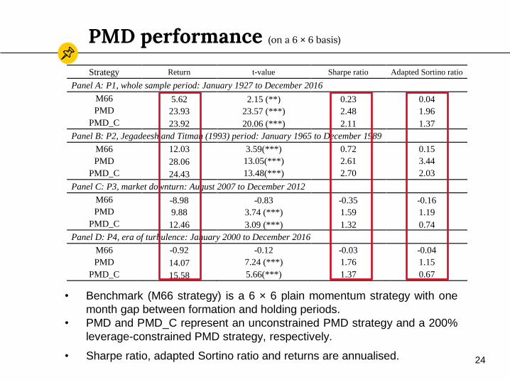
PMD performance (on a 6 × 6 basis)
Strategy Return t-value Sharpe ratio Adapted Sortino ratio
Panel A: P1, whole sample period: January 1927 to December 2016
M66 5.62 2.15 (**) 0.23 0.04
PMD 23.93 23.57 (***) 2.48 1.96
PMD_C 23.92 20.06 (***) 2.11 1.37
Panel B: P2, Jegadeesh and Titman (1993) period: January 1965 to December 1989
M66 12.03 3.59(***) 0.72 0.15
PMD 28.06 13.05(***) 2.61 3.44
PMD_C 24.43 13.48(***) 2.70 2.03
Panel C: P3, market downturn: August 2007 to December 2012
M66 -8.98 -0.83 -0.35 -0.16
PMD 9.88 3.74 (***) 1.59 1.19
PMD_C 12.46 3.09 (***) 1.32 0.74
Panel D: P4, era of turbulence: January 2000 to December 2016
M66 -0.92 -0.12 -0.03 -0.04
PMD 14.07 7.24 (***) 1.76 1.15
PMD_C 15.58 5.66(***) 1.37 0.67
• Benchmark (M66 strategy) is a 6 × 6 plain momentum strategy with one
month gap between formation and holding periods.
• PMD and PMD_C represent an unconstrained PMD strategy and a 200%
leverage-constrained PMD strategy, respectively.
• Sharpe ratio, adapted Sortino ratio and returns are annualised. 24

Comparison of performance (PMD strategies versus
the Barroso and Santa-Clara (2015) volatility-scaled momentum strategy)
• Benchmark (WML strategy) is an 11 × 1 plain
momentum strategy with one month gap between
formation and holding periods.
• PMD and PMD_C represent an unconstrained
PMD strategy and a 200% leverage-constrained
PMD strategy, respectively.
• BSC represents the volatility-scaled momentum
strategy constructed by Barroso and Santa-Clara
(2015).
• Sharpe ratio, adapted Sortino ratio and returns are
annualised. 25

Comparison of performance (PMD strategies versus
the Barroso and Santa-Clara (2015) volatility-scaled momentum strategy)
Strategy Return t-value Sharpe ratio Adapted Sortino ratio
P1: whole sample period: January 1927 to December 2016
WML 19.05 5.58 (***) 0.59 0.24
BSC 17.30 8.82 (***) 0.94 1.04
PMD 28.16 24.28 (***) 2.56 2.16
PMD_C 27.47 21.47 (***) 2.26 1.51
P2: Jegadeesh and Titman (1993): January 1965 to December 1989
WML 29.75 5.98 (***) 1.20 0.54
BSC 26.52 6.32 (***) 1.26 1.22
PMD 35.13 14.59 (***) 2.92 2.60
PMD_C 30.17 14.75 (***) 2.95 1.90
P3: market downturn: August 2007 to December 2012
WML 1.46 0.08 0.03 0.01
BSC 11.83 1.88 (*) 0.80 0.98
PMD 13.87 3.94 (***) 1.68 0.98
PMD_C 19.06 3.14 (***) 1.34 0.66
P4: era of turbulence: January 2000 to December 2016
WML 7.82 0.79 0.19 0.08
BSC 5.40 1.64 0.40 0.38
PMD 16.19 6.64 (***) 1.61 1.03
PMD_C 19.44 5.54 (***) 1.34 0.76
26
See BSC(2015)table 3,page 116.
International Evidence
• Consistent with Daniel and Moskowitz (2016), we use
the Asness, Moskowitz, and Pedersen (2013) “P3-P1”
momentum portfolios obtained from the AQR Data
Library. We refer to it as WML_T.
• We report PMM and PMD performances for the UK,
Japan and Europe along with the US over 1972–2016.
AMP (2013) “P3-P1” momentum portfolios
• Data sourced from DataStream and XpressFeed Global.
• Tercile sort rather than decile sort.
• Large and liquid stocks only. The universe of stocks that account
cumulatively for 90% of the total MV of the entire stock market.
(similar to how MSCI defines for its global stock indices)
• Average no. of stocks: 724 (US), 147 (UK), 290 (Europe), and
471 (Japan).27

International Evidence
28
Other robustness checks
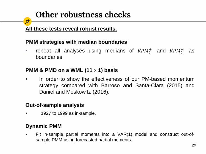
All these tests reveal robust results.
PMM strategies with median boundaries
• repeat all analyses using medians of 𝑅𝑃𝑀𝑡+ and 𝑅𝑃𝑀𝑡
− as
boundaries
PMM & PMD on a WML (11 × 1) basis
• In order to show the effectiveness of our PM-based momentum
strategy compared with Barroso and Santa-Clara (2015) and
Daniel and Moskowitz (2016).
Out-of-sample analysis
• 1927 to 1999 as in-sample.
Dynamic PMM
• Fit in-sample partial moments into a VAR(1) model and construct out-of-
sample PMM using forecasted partial moments.29

Practical Matters
1. No transaction costs.
2. No consideration of tradability and liquidity.
If it is in CRSP, we use it. Maybe ok for
factor but not for strategy. Methods used
for international evidence might be more
practical.
30

Topic 3
Distribution of CSM Returns
Oh Kang Kwon a and Stephen Satchell a,b
Prensented by: Stephen Satchell
a University of Sydney Business School b Trinity College, University of Cambridge
31
The Distribution of CSM returns
• Assumes returns on stocks are multivariate normal.
• Treats the problem as two-period, the formation and
holding period.
• If two periods are independent and returns
stationary, then markets efficient and high
momentum returns a consequence of , presumably
higher risk.
• Paper addresses what the distribution of CSM
returns actually is.
• This has implications for payouts that CSM
investors will experience.
32

The Distribution of CSM returns
• Portfolios considered as m long, m short, universe n; Suppose
n=2, m=1.
• If in formation period t: 𝑟1𝑡 > 𝑟2𝑡, go long asset 1, short 2;
If 𝑟1𝑡 < 𝑟2𝑡 , do opposite.
• 𝑃𝑑𝑓(𝑟𝑚𝑡+1) = 𝑃𝑑𝑓 𝑟1𝑡+1 − 𝑟2𝑡+1 𝑎𝑛𝑑 𝑟1𝑡 > 𝑟2𝑡;
+𝑃𝑑𝑓(𝑟2𝑡+1 − 𝑟1𝑡+1 𝑎𝑛𝑑 𝑟1𝑡 < 𝑟2𝑡;)
• If markets are efficient; this becomes a mixture of univariate
normals, in this case kurtotic and left skewed for plausible values:
𝑃𝑑𝑓(𝑟𝑚𝑡+1) = 𝑃𝑑𝑓 𝑟1𝑡+1 − 𝑟2𝑡+1 )𝑃𝑟𝑜𝑏( 𝑟1𝑡 > 𝑟2𝑡;
+𝑃𝑑𝑓(𝑟2𝑡+1 − 𝑟1𝑡+1 )𝑃𝑟𝑜𝑏(𝑟1𝑡 < 𝑟2𝑡;)
• If markets not efficient (predictable) structure is more complicated
but describable in terms of truncated bivariate normal
distributions.33

Mixtures of Distributions
• What are they?
• Imagine you toss a coin first
• Then if heads you get N(0,1)
• Then if tails you get N(5,10)
• The resulting pdf is a mixture of normals
34
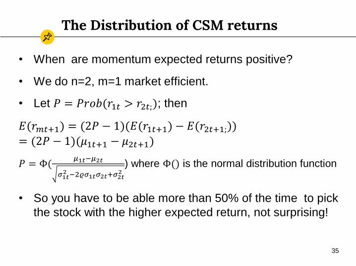
The Distribution of CSM returns
• When are momentum expected returns positive?
• We do n=2, m=1 market efficient.
• Let 𝑃 = 𝑃𝑟𝑜𝑏(𝑟1𝑡 > 𝑟2𝑡;); then
𝐸(𝑟𝑚𝑡+1) = (2𝑃 − 1)(𝐸(𝑟1𝑡+1) − 𝐸(𝑟2𝑡+1;))
= (2𝑃 − 1)(𝜇1𝑡+1 − 𝜇2𝑡+1)
𝑃 = Φ(𝜇1𝑡−𝜇2𝑡
𝜎1𝑡2 −2𝜚𝜎1𝑡𝜎2𝑡+𝜎2𝑡
2) where Φ() is the normal distribution function
• So you have to be able more than 50% of the time to pick
the stock with the higher expected return, not surprising!
35

The Distribution of CSM returns
• Would high CSV be good/bad for CSM?
• This depends upon whether it is factor CSV(good)
or idiosyncratic CSV(bad)
• We can see this from previous formula, factor CSV
increases the numerator, other the denominator.
36

The Distribution of CSM returns
• All the above generalise: for n assets, m, long m
short we need to know the number of possible
rankings each of which contribute to the pdf of
momentum. This number is𝑛!
𝑛−2𝑚 !𝑚!𝑚!.
• So if we want to investigate S&P500 long top 100
short bottom 100, we get a vast number but
previous pdf generalises. We get𝑛!
𝑛−2𝑚 !𝑚!𝑚!terms
in the pdf which involve univariate normals and
truncated high dimensional multivariates.
37

Result
38
• The result is that the density consists of a very large
number of components.
• The case of 2 assets, it has 2 components (see slide 35).
• The case of N assets, it has𝑛!
𝑛−2𝑚 !𝑚!𝑚!components (see
slide 37).

Complexity
• The notion that expected utility maximisers take expected
values over such a distribution becomes fanciful without
access to modern MC.
• Consider500!
400 !50!50!, this is huge, the age of the universe
is 13,800,000,000 years the number of seconds in history
is exp(40) the number of pdfs the EU maximiser needs to
consider is exp 320 .
39

Conclusions
• We started arguing against BF.
• We derived the pdf of CSM which gives us some insights
into more complex cases.
• We ended up questioning expected utility.
40

Any questions ?
Thanks!
Stephen Satchell
University of Sydney Business SchoolTrinity College, University of Cambridge [email protected]
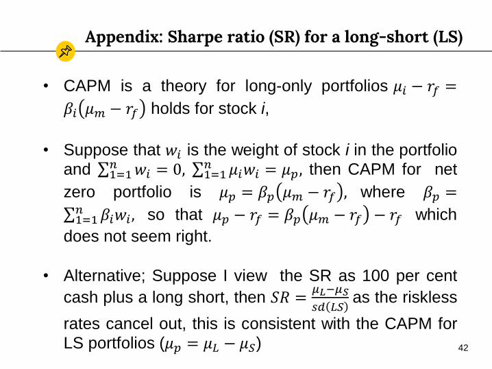
Appendix: Sharpe ratio (SR) for a long-short (LS)
• CAPM is a theory for long-only portfolios 𝜇𝑖 − 𝑟𝑓 =
𝛽𝑖 𝜇𝑚 − 𝑟𝑓 holds for stock i,
• Suppose that 𝑤𝑖 is the weight of stock i in the portfolio
and σ1=1𝑛 𝑤𝑖 = 0, σ1=1
𝑛 𝜇𝑖𝑤𝑖 = 𝜇𝑝, then CAPM for net
zero portfolio is 𝜇𝑝 = 𝛽𝑝 𝜇𝑚 − 𝑟𝑓 , where 𝛽𝑝 =
σ1=1𝑛 𝛽𝑖𝑤𝑖 , so that 𝜇𝑝 − 𝑟𝑓 = 𝛽𝑝 𝜇𝑚 − 𝑟𝑓 − 𝑟𝑓 which
does not seem right.
• Alternative; Suppose I view the SR as 100 per cent
cash plus a long short, then 𝑆𝑅 =𝜇𝐿−𝜇𝑆
𝑠𝑑 𝐿𝑆as the riskless
rates cancel out, this is consistent with the CAPM for
LS portfolios (𝜇𝑝 = 𝜇𝐿 − 𝜇𝑆) 42