Embed Size (px)
Citation preview
Cross-Autocorrelation of Dual-Listed Stock Portfolio Returns: Evidence from the Chinese Stock Market
Mr. DAXUE WANG
IESE Business School Av. Pearson 21
Barcelona, 08034 Spain E-mail: [email protected]
Tel.: 34-645993771
ABSTRACT
In this paper, we apply a GARCH model to examine the cross-autocorrelation pattern between daily returns of portfolios composed of dual-listed stocks in Chinese stock market, before and after China opened its once foreign-exclusive B-share market. A lead-lag relationship between the A-share and B-share portfolio returns is identified during our sample periods, with the A-share portfolio leading the B-share portfolio. Upon the opening of B-share market, a change from underreaction to overreaction is found in the response pattern of B-share market, producing a rarely seen negative cross-autocorrelation. The results of two additional tests are reported. First, by decomposing the portfolio return into portfolio-specific and market-wide returns, we find that the market-wide information contained in A-share portfolio return is strongly associated with the cross-autocorrelation structure. Second, we document a directional asymmetry in which B-share portfolio shows either slow or over response to bad, but not good, news of A-share portfolio. We conclude that information asymmetry alone is not enough to explain the lead-lag relationship, and investor behavior must be taken into consideration. [JEL G14, G18]
Keywords: Cross-Autocorrelation; Segmented Stock Markets; Dual-Listed Stocks; Market-Wide and Portfolio-Specific Information.

2
I. Introduction
Efficient market hypothesis suggests that financial asset returns should not be predictable
based on all publicly available information. However, the existence of the asymmetric
cross-autocorrelation between large and small market capitalization portfolios has been
well documented in U.S. stock market by Lo and MacKinlay (1990). Their study indicates
that short-horizon returns on the portfolio of stocks with large market capitalization predict
those with smaller market capitalization better than vice versa. This asymmetric cross-
autocorrelation is called the lead-lag effect. Similar pattern has been identified in other
markets, such as several Asian markets (Chang et al., 1999), United Kingdom (Kanas and
Kauretas, 2001), German and Turkish (Altay, 2003), and Brazil (Ratner and Leal, 2003). 1
Cross-autocorrelation may account for a large percent of some documented contrarian
profits. If returns on some stocks systematically lead or lag those of others, rational
investors can condition their leading shares’ trading decisions on the previous price
movement of lagged shares, and a portfolio strategy that sells “winners” and buys “losers”
can produce positive expected returns. Several explanations have been proposed for the
lead-lag effect structure, including information adjustment asymmetry (Chan, 1993;
Badrinath et al., 1995), nonsynchronous trading (Boudoukh et al., 1994), transaction costs
(Mench, 1993; Bernhardt and Mahani, 2004), and contemporaneous correlations (Hameed,
1997).
The information adjustment asymmetry, emphasizing the differences in the speeds of asset
price adjustment processes to information, is the most popular explanation. According to
Chan (1993), if market makers observe noisy signals about their stocks and correct pricing
errors by observing the additional signals inferred from previous price changes in other
stocks, then stock returns become positively cross-autocorrelated. The signal quality
differences among stocks could cause the asymmetric cross-autocorrelation. As a result, if
there is higher-quality information in large stocks than in small stocks, possibly due to the
lower marginal costs of producing information, as proposed by Ho and Michaely (1988),
then the returns of large stock portfolios would lead that of small stock portfolios. 1 The six Asian stock markets are Hong Kong, Japan, Singapore, South Korea, Taiwan, and Thailand.

3
Badrinath et al. (1995) associate cross-autocorrelation with the institutional ownership of
the stocks. The institutional investors concentrate on specific groups of stocks, usually large
capitalized ones, and produce more information about these stocks. Then the price change
of the informational favored stocks produce additional signal for other informational
unfavored ones.
According to nonsynchronous trading, cross-autocorrelation relationship results from the
assumption that multiple time series are sampled simultaneously when in fact they are
nonsynchronous, which induces spurious cross-effects among stocks. Lo and MacKinlay
(1990) conclude that unrealistically thin markets are required for the noncynchronous
trading to explain the observed cross-autocorrelation; however, Boudoukh et al. (1994)
argue that Lo and MacKinlay seriously understate the potential effects of nonsynchronous
trading. Actually, the nonsynchronous trading and the information asymmetric pattern do
not have to be exclusive to each other in explaining the cross-autocorrelation. As Bernhardt
and Davies (2005) indicate, the prices of less active stocks do not incorporate some of the
recent information that is already contained in the prices of more active stocks. As a
specific case, the trading of small stocks is mostly thinner than that of large stocks, with a
result that last transactions of small stocks on any trading day are usually completed before
those of large stocks. Therefore, the price of large stocks will likely reflect any news
arriving in the market toward the end of the trading day, while the price of small stocks will
only show the effect of this information on the following day.
Mench (1993) lists transaction costs, low transactions and market microstructure as the
reasons of the cross-autocorrelation. Bernhardt and Mahani (2001) show that, on top of
information asymmetry, additional friction such as transaction costs is necessary to explain
the cross-autocorrelation pattern. They offer a model with non-fundamental speculation
featured with a common liquidity-traded component and agents with information related to
liquidity trade. With this model, negative cross-autocorrelation is possible.
As an opposing view from the above mentioned authors, Hameed (1997) argues that the
portfolio cross-autocorrelation is simply a restatement of portfolio autocorrelations, and
once portfolio autocorrelations are taken into account, the cross-autocorrelation should
disappear.

4
Should these reasons exist behind the lead-lag effect, then the cross-autocorrelation pattern
applies to segmented financial markets, where various types of shares of the same stock are
issued and different shareholders have different access to market segmentation. Chui and
Kwok (1998) test the Chinese A-share and B-share markets, and they find that B-share
market leads A-share market during the period of 1993-1996. Two factors are reported to
account for the phenomena: the mechanism of information transmission and differences
between market participants. More specifically, A-shares are mainly traded by domestic
individual investors, compared to the majority of foreign institutional investors in B-share
market, who are more likely to have more advanced technology for processing and
analyzing information. In addition, foreign investors get information from the free market
of Hong Kong, while domestic investors are constrained by the mainland media and
publishing industry which is under firm controls of central government. Accordingly,
public information is expected to reach the B-share market before the A-share market.
However, whether foreign investors in China possess information advantage deserves
closer examinations. The existence of information asymmetry on values of local assets
between foreign investors and domestic investors has been documented extensively in
Brennan and Cao (1997), Stulz and Wasseerfallen (1995), and Kang and Stulz (1997). It is
typically assumed by the literature that domestic investors are better informed than foreign
investors. The case is confirmed in Chinese market by Chakravarty et al. (1998), and Su
and Fleisher (1999). The reasons they provide include language barriers, different
accounting standards, and a lack of reliable information about the local economy and firms
available to foreign investors. On top of this, the trading of a B-share stock is usually much
thinner than that of its A-share counterpart. So the conclusion of Chui and Kwok (1998) is
subject to further testing.
The main purpose of this paper is three-fold. First, we re-examine the cross-autocorrelation
pattern in Chinese stock market with the portfolios of dual-listed stocks. Second, we test the
impacts of China’s opening of its once foreign-exclusive B-share market to its domestic
individual investors. In February 2001, Chinese government announced that domestic
individual investors were permitted to invest in B-shares. Accordingly, the cross-
autocorrelation between A- and B-shares, if they existed, might have changed. Third, we

5
explore the sources of the lead-lag pattern. The paper will shed lights on both the policy
making and the investment strategy of active traders in segmented stock markets.
The remainder of this paper is organized as follows. Section II describes the data and
sample selection. Section III examines the general cross-autocorrelation pattern. Section IV
evaluates the relative importance of various components by decomposing the portfolio
returns. Section V proposes the potential reasons behind the empirical results. The paper
ends with a brief summary of conclusions.
II. Data and Sample Selection
Chinese stock market was established in early 1990s. Over the past decade, it has
undergone a substantial increase and become the second largest stock market in Asia.
Despite the rapid growth, the market remains underdeveloped in many senses. For instance,
Greonewold et al. (2001) study the efficiency of the market. They find evidence of
departures from weak and semi-strong form efficiency in the sense that predictability of
security returns can be obtained on the basis of their own past values.
A distinguishing feature of Chinese stock market is the privilege listed companies have,
upon meeting certain requirements, of issuing either A-shares or B-shares that can be freely
traded.2 A-shares are denominated in RMB, and B-shares are denominated in US Dollar
(Shanghai Stock Exchange, SSE) or HK Dollar (Shenzhen Stock Exchange, SHSE). Other
than who can own them, these shares are legally identical, with the same voting rights and
dividends. Before February 2001, China’s stock market was listed by International Finance
Corporation as the only equity market with completely segmented trading between
domestic and foreign investors, since A-shares were traded among P.R. China citizens,
while B-shares were traded among non-P.R. China citizens. Two measures have been taken
in the Chinese market to break the segmentation. First, since February 19, 2001, domestic
individuals with legal foreign exchanges have been permitted to trade B-shares, but not the
vice versa. Second, in December 2002, QFII (Qualified Foreign Institutional Investors) was
introduced in the market, with the hope that foreign investment institutions will spur on 2 In addition to A-share and B-shares, a Chinese company can also issue H- and N-shares in Hong Kong and New York, respectively. There are also some state owned Chinese companies incorporated and listed in Hong Kong that have the name of “red chips”.
6
better and more effective functioning. Under QFII, certain foreign institutional investors
have been allowed to trade in A-share market. 3
We obtain daily adjusted price of stocks dual-listed in both A-share and B-Share markets of
SSE and SHSE from Datastream, covering the period between January 1, 1995 and
September 30, 2005. This timeframe effectively avoids the infancy period of the Chinese
stock market and the RMB’s foreign exchange rate adjustment period in 1994. To test the
structural change brought by China’s opening its once foreign-only shares to domestic
individual investors, we divide the total sample period into two subperiods: January 1, 1995
- January 31, 2001 (PRE-FEB) and February 1, 2001 - September 30, 2005 (POST-FEB).
The sample population consists of 72 pairs of firms, which form A-share portfolio and B-
share portfolio on an equal-weighted basis. Since the portfolios are formed by dual-listed
stocks, we diminish the influence of factors associated with stock-specific components. For
a stock to be included into the portfolio on a specific day, both its A-share and B-share
must be traded on that day; otherwise, the stock is excluded. In order to reduce the IPO
under-pricing effect documented by Mok and Hui (1998), the first 20 days trading data
following the IPO of each stock are removed. The descriptive statistics for the portfolio in
the sample period is reported in Table 1. 4
# Insert Table 1 about here #
From Table 1, the returns of the portfolios appear non-normally distributed with fat-tail
over various time horizons, except the monthly return for the A-share portfolio. Longer
horizon returns appear more normal than shorter horizon returns for A-share portfolio, but
not for B-share portfolio.
3 Until June 30, 2005, twenty-seven companies have acquired licenses, with a combined US$4 billion investment quota to buy A-shares, bonds and mutual funds. As of September 30, 2005, seventeen of these companies are investing in A-share stocks. 4 Here, portfolio returns are calculated first from simple returns and then are converted to continuously compounded returns. The weekly return of each security is computed as the return from Tuesday’s closing price to the following Tuesday’s closing price. If the following Tuesday’s price is missing, then Wednesday’s price (or Monday’s price, if Wednesday’s price is also missing) is used. If both Monday’s and Wednesday’s prices are missing, then the return for that week is reported as missing. The monthly return of each security is computed as the return from the closing price of the last trading day of the month to that of the following month.

7
Except the PRE-FEB subperiod, the B-share portfolio has a higher average return than the
A-share portfolio, followed by its total higher risk levels.
Table 2 exhibits the autocorrelation for daily, weekly and monthly portfolio returns over the
sample periods. A significant first order autocorrelation can be observed for daily returns of
both portfolios, with smaller and sometimes negative high-order autocorrelations.5 The
weekly and monthly return autocorrelations reported in panel B and C of Table 2 exhibit
different patterns: mixed sign and statistically insignificant at the first lag over the entire
periods for A-share portfolio, while positive and mixed statistically significance for B-share
portfolio. The evidence indicates that information on own price transmits faster in A-share
market than in B-share market.
# Insert Table 2 about here #
III. General Cross-Autocorrelation Pattern
In this section, we study the general cross-autocorrelation pattern between A-share and B-
share portfolios. Then, we check the structural change of the pattern before and after the B-
share market opening in February 2001. We focus on several propositions, which are tested
with associated models.
3.1 General Cross-Autocorrelation Structure
Our first two propositions are built as follows:
Proposition 1: The cross-autocorrelation between the return of B-share portfolio on day (t-
1) and that of A-share portfolio on day t is significant.
Proposition 2: The cross-autocorrelation between the return of A-share portfolio on day (t-
1) and that of B-share portfolio on day t is significant.
The two propositions imply that A-share and B-share investors of the same stock could gain
information from each other.
5 Several explanations about the portfolio autocorrelations has been offered in finance literature (Mench, 1993), including the slow adjustment of stock price to new information, autocorrelation in the underlying expected returns, and mispricing.

8
We use the following model with GARCH (Generalized Autoregressive Conditional
Heteroskedasticity) disturbance to approximate the return generating process of A-share
and B-share portfolios. To diminish the impact of own autocorrelation, we include the
lagged return of each portfolio in explaining its return.
tAtAAAtBABAtA RRR ,1,1,, εββα +++= −−
tAtAtA ,,, μσε = , 21,1,
21,1,0,
2, −− ++= tAAtAAAtA σωεγγσ (1)
tBtBBBtABABtB RRR ,1,1,, εββα +++= −−
tBtBtB ,,, μσε = , 21,1,
21,1,0,
2, −− ++= tBBtBBBtB σωεγγσ (2)
where tAR , ( tBR , ) is the A-share (B-share) portfolio return at time t, ABβ ( BAβ ) is the
sensitivity of A-share (B-share) portfolio return on one-day lagged B-share (A-share)
portfolio return, AAβ ( BBβ ) is the sensitivity of A-share (B-share) portfolio return on its own
one-day lagged return, Aα ( Bα ) is the regression coefficient of the A-share (B-share)
portfolio return, tA,ε ( tB,ε ) is the error term, and }{ ,tAμ and }{ ,tBμ are both sequences of
independent and identically distributed random variables with mean zero and variance 1.
In the model, a positive ABβ implies that A-share portfolio partly reacts to the B-share
portfolio return with a lag, while a negative ABβ implies that A-share portfolio overreacts to
the B-share portfolio return and this overreaction gets corrected in the subsequent period.
The same implications apply to B-share portfolio as well.
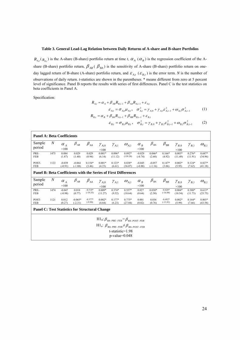
The statistical results of the model are reported in table 3. Consistent with Richardson and
Peterson (1999) but inconsistent with Hameed (1997), the cross-autocorrelation effect is
significant after taking the autocorrelation effect into account.
# Insert Table 3 about here #
In the PRE-FEB subperiod, BAβ is larger than zero at 5% significant levels (t-statistic of
2.60), i.e., there is a positive and statistically significant one-day lagged effect of A-share
portfolio returns on B-share portfolio returns. On the contrary, we do not observe the
significant lagged effect of B-share portolio return on A-share portfolio returns (t-statistic

9
of 1.40). For the POST-FEB subperiod, the correlation changes its sign and there is no
evidence of significant one-day lagged effect on B-share portfolio returns (t-statistic of -
1.16). In this subperiod, we do not observe the lagged effect on A-share portfolio returns
either. So, for both subperiods, we reject Proposition 1, but not Proposition 2 for the PRE-
FEB subperiod, at 5% significant level. In other words, the evidence is consistent with Chui
and Kwok (1998) in that the cross-autocorrelation of the portfolio returns is asymmetric,
but inconsistent with Chui and Kwok in that the returns of A-share portfolio lead those of
B-share portfolio.
Figure 1 shows the evolution of 2,tAσ and 2
,tBσ , variance of residuals in Eq. 1 and Eq. 2,
respectively. The correlation between 2,tAσ and 2
,tBσ is 0.126, and we do not find strong co-
movement between the residual variances.
0.0
02.0
04.0
06.0
08.0
1V
aria
nce
08/95 05/98 01/01 10/03 07/06Date
varianceA varianceB
Figure 1. Co-evolution of residual variances
To check the possible spurious correlations between the portfolio returns, we run the
regression of the equations with the first differences of the series. We define the first
differences of the portfolio return series as )( 1,,, −−=Δ tAtAtA RRR and )( 1,,, −−=Δ tBtBtB RRR ,
and replace tAR , , tBR , , 1, −tAR , and 1, −tBR in Eq.1&2 with tAR ,Δ , tBR ,Δ , 1, −Δ tAR and 1, −Δ tBR ,
respectively. Through the results reported in Panel B of Table 3, we find that correlations
between the first differences almost keep the original level of significance, so we conjecture
that the correlations in the portfolio returns are not spurious.

10
3.2 The Effect of Financial Policy on the Cross-Autocorrelation Structure
Regarding the effects of the B-share market opening on the cross-autocorrelation pattern,
we establish the following proposition.
Proposition 3: The leading pattern of A-share portfolio return on B-share portfolio return
has significantly changed after the opening policy.
To test the proposition, we set FEBPREBA −−β = FEBPOSTBA −−β as the null hypothesis and
FEBPREBA −−β ≠ FEBPOSTBA −−β as the alternative hypothesis. The alternative hypothesis implies the
lead effect of A-share portfolio returns on that of B-share portfolio returns has changed
after February, 2001.
The results are shown in panel C of Table 3. The t-statistic of 1.98 on the difference
between FEBPREBA −−β and FEBPOSTBA −−β is significant at the 5% level, so we do not reject
Proposition 3, i.e., a significant change is found in the cross-autocorrelation pattern.
IV. Cross-Autocorrelation Pattern with Decomposed Returns
In section 3, we conclude that there is a general lead-lag pattern of the A-share and B-share
portfolio returns, with the former leading the latter. In this section, by decomposing the
portfolio returns into portfolio-specific and market-wide components, we study the effects
of the market information on lead-lag pattern. We also study the speed of B-share portfolio
returns in responding the lagged good news and bad news from A-share portfolio. By doing
so, we can further identify the source of the lead-lag effect.
4.1 Market-Wide and Portfolio-Specific Information
In order to decompose the total portfolio returns into market-wide and portfolio specific
components, we use the following equation as an estimation of the CAPM:
tAtMAtA RR ,,, εβα ′+∇+=∇
),0(~ 2, φε NtA′ (3)
where tr is the return on a risk-free asset at time t, tAR ,∇ (= ttA rR −, ) and tMR ,∇ (= ttM rR −, )
are the excess return on A-share portfolio and the market portfolio at time t, respectively,

11
Aβ is the sensitivity of excess A-share portfolio return on the market portfolio return, α is
the regression coefficient, and tA,ε ′ is the error term. In estimating the model, Datastream
China Country Price Index and China Time Deposit are used as the proxies for market
portfolio and the risk-free asset, respectively.
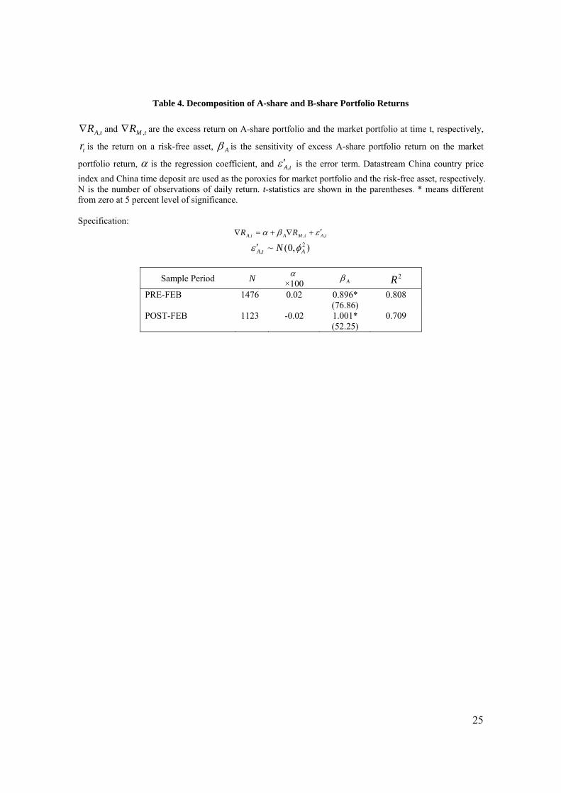
The statistical results are reported in Table 4. From the table, market beta coefficients are
highly significant in both subperiods. The explanation power of the model is also high, with
an R2 over 0.7.
# Insert Table 4 about here #
Since the risk-free interest rate and the constant of Eq. 3 are very small, we use the error
term tA,ε ′ estimated by the above CAPM as portfolio-specific returns in testing the effect of
the lagged A-share portfolio-specific information on B-share portfolio returns. Similarly,
the systematic return, MtAR , ( tAtAR ,, ε ′−= ), can be used as the indicator of market-wide
information in the cross-autocorrelation structure.6
The following GARCH (1, 1) model is used to test the effects of lagged A-share portfolio-
specific and market-wide information on the B-share portfolio return:
tBtBBB
MtA
MBAtA
PBABtB RRR ,1,1,1,, εββεβα +++′+= −−−
tBtBtB ,,, μσε = , 21,1,
21,1,0,
2, −− ++= tBBtBBBtB σωεγγσ (4)
where tA,ε ′ is the one-day lagged A-share portfolio-specific return, M
tAR 1, − is the one-day
lagged systematic return of A-share portfolio, PBAβ ( M
BAβ ) is the sensitivity of B-share
portfolio return to one-day lagged A-share portfolio-specific (systematic) return, and the
other variables with the same implication as Eq. 2.
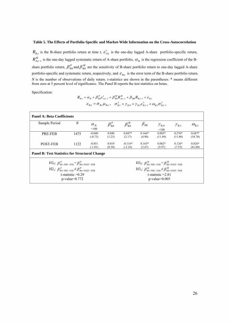
The summary statistics of the system estimation are reported in Table 5. From the table,
one-day lagged market-wide information reflected in A-share portfolio returns has a
6 We try decomposing the portfolio return (not the excess return) with a one-factor model:
tAtMAAtA eRbR ,,, ++= μ , where Aμ represents the expected components, tMARb , the unexpected market-wide
component, and tAe , the unexpected portfolio-specific component. We run the regression and get similar results which do not affect our conclusions. Therefore, we only report the results based on the CAPM.
12
significant effect on B-share portfolio returns in both subperiods (t-statistic of 2.17 for the
PRE-FEB subperiod and -2.16 for the POST-FEB subperiod), while the A-share portfolio-
specific information does not have any statistically significant effect on the B-share
portfolio returns (t-statistic of 1.23 for the PRE-FEB subperiod and 0.30 for the POST-FEB
subperiod). This evidence shows that the general significant cross-autocorrelation between
A-share and B-share portfolios is due to the market-wide information content of A-share
portfolio returns, as predicted from Chan (1993).
# Insert Table 5 about here #
A further test in Panel B of Table 5 shows that the difference of the MBAβ between PRE- and
POST-FEB subperiods is significant (t-statistic of 2.81), but it is not the case for PBAβ (t-
statistic of 0.29). The B-share portfolio return tends to underreact to the market-wide
information contained in the A-share portfolio in the PRE-FEB subperiod but overreact in
the POST-FEB subperiod.
4.2 Directional Asymmetry with Down and Up Market
McQueen et al. (1996) employ a methodology of directional asymmetry to further analyze
the cross-autocorrelation structure of the size-sorted portfolios in NYSE. They find that
small and large cap portfolios’ reactions to bad news are fast, but the reactions of small cap
portfolio to good news are slower than that of the large cap portfolio. Chang et al. (1998)
find that the good news and bad news pattern is not universal across Asian markets.
Here we examine the reactions of B-share portfolio returns to increasing and decreasing
lagged A-share portfolio returns. Like McQueen et al. (1996), we decompose the
systematic component of A-share portfolio returns into two different new time series: First
series, upward returns, equal to the original returns when they take positive values and zero
otherwise; second series, downward returns, equal to the original returns when they take
negative values and zero otherwise. The decomposition produces the following two series:
⎩⎨⎧ >
= −−− otherwise
RifRR
MtA
MtAuM
tA ,00, 1,1,,
1,
13
⎩⎨⎧ <
= −−− otherwise
RifRR
MtA
MtAdM
tA ,00, 1,1,,
1,
We estimate the pattern with the GARCH (1, 1) model:
tBtBBBdM
tAdBA
uMtA
uBAtA
PBABtB RRRR ,1,
,1,
,1,1,, εβββεβα ++++′+= −−−−
tBtBtB ,,, μσε = , 21,1,
21,1,0,
2, −− ++= tBBtBBBtB σωεγγσ (5)
where uM
tAR ,1, − ( dM
tAR ,1, − ) is the one-day lagged upward (downward) systematic return of A-share
portfolio, uBAβ ( d
BAβ ) is the sensitivity of B-share portfolio systematic return to one-day
lagged upward (downward) returns of A-share portfolio, and the other variables with the
same implication as Eq. 2.
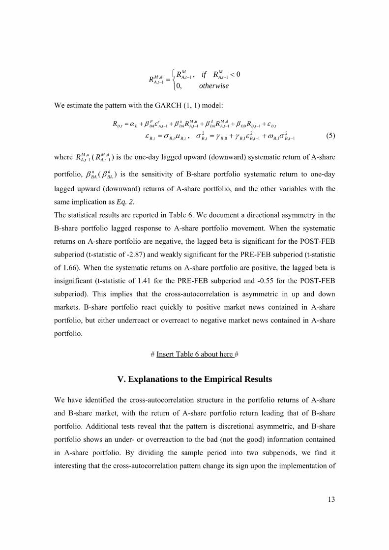
The statistical results are reported in Table 6. We document a directional asymmetry in the
B-share portfolio lagged response to A-share portfolio movement. When the systematic
returns on A-share portfolio are negative, the lagged beta is significant for the POST-FEB
subperiod (t-statistic of -2.87) and weakly significant for the PRE-FEB subperiod (t-statistic
of 1.66). When the systematic returns on A-share portfolio are positive, the lagged beta is
insignificant (t-statistic of 1.41 for the PRE-FEB subperiod and -0.55 for the POST-FEB
subperiod). This implies that the cross-autocorrelation is asymmetric in up and down
markets. B-share portfolio react quickly to positive market news contained in A-share
portfolio, but either underreact or overreact to negative market news contained in A-share
portfolio.
# Insert Table 6 about here #
V. Explanations to the Empirical Results
We have identified the cross-autocorrelation structure in the portfolio returns of A-share
and B-share market, with the return of A-share portfolio return leading that of B-share
portfolio. Additional tests reveal that the pattern is discretional asymmetric, and B-share
portfolio shows an under- or overreaction to the bad (not the good) information contained
in A-share portfolio. By dividing the sample period into two subperiods, we find it
interesting that the cross-autocorrelation pattern change its sign upon the implementation of

14
the B-share opening policy by Chinese government. In this section, we will provide
analysis to these findings.
5.1 Market Microstructure
We start by examining the reasons listed by Chui and Kwok (1998) concerning the
information transmission mechanism in Chinese stock market.
At the early stage, there had been a sharp contrast between A-share and B-share market
participants. Most traded A-shares were held by small retail investors, since there were
relatively few large Chinese institutional investors; by contrast, B-shares were traded by
institutional foreign investors such as mutual funds. So it is safe to say that domestic
individual investors dominated the A-share market, while foreign institutional investors
dominated the B-share market at that stage. However, the situation has changed since the
Asian financial crisis in 1998, when the institutional foreign investors started to quit the
market. Restrictions on foreign ownership and little control over poorly-performing
enterprises had led to disappointing results for the B-share market long before February
2001. The Economist (March 3, 2001) and the Asian Wall Street Journal (February 21,
2001) suggest that by early 2001, 60 to 80 percent of B shares were held illegally by
Chinese residents. The situation has been deteriorated after the implementation of B-share
opening policy. On the other side, in late 2002, large foreign investors were allowed to
trade in A-share market according to QFII, which has changed the investor profile in both
A-share and B-share markets further.
Additionally, even though the media and publishing industry is still under monopoly in
China through inspection systems, the entry of WTO and widespread use of internet has
destroyed the advantages of foreign investors described by Chui and Kwok, if any.
Chakravarty et al. (1998) argue that domestic investors tend to have access to more
information than B-share investors even before 1998. In addition, the disclosure in B-share
market is far from satisfactory. It has been much less studied by institutional investors,
reflecting the fact that it is even harder to find a company research report on B-share market.
Thus we believe that A-share investors get access to information faster than B-share
investors, as reflected in the observed lead-lag pattern.

15
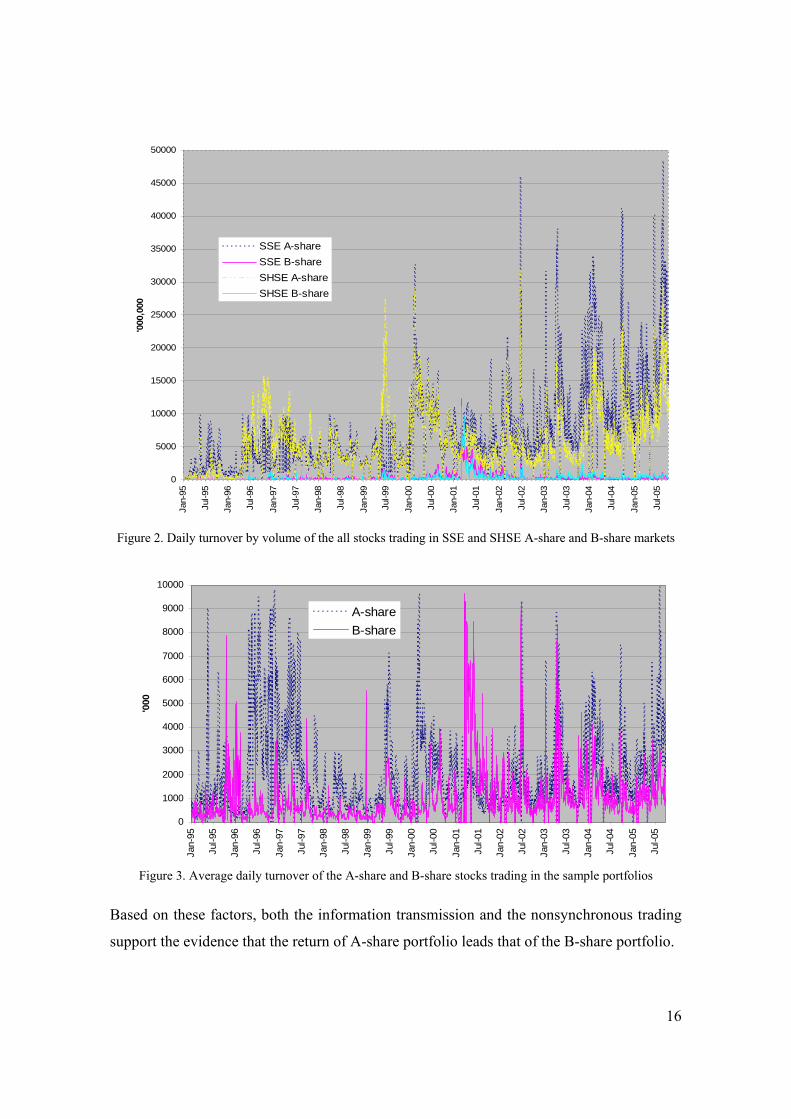
Finally, the difference of liquidity between the A-share and B-share markets also support
the lead-lag pattern. The B-share market has expanded far less rapidly than the A-share
market, in terms of issued shares, market capitalization, and number of companies. Figure 2
shows the movement of daily turnover (by volume) of the all stocks in SSE and SHSE A-
share and B-share markets during the sample period. From the figures, we can easily tell
that the B-share market has far less liquidity than A-share market. In the whole sample
period, only in early 2001 has B-share market recorded turnovers that approximated those
of A-share market. More specifically, Figure 3 shows the movement of average daily
turnover (by volume) of the 58 pairs of A-share and B-share stocks in the sample portfolios
during the sample period. Not surprisingly, the turnovers of B-share stocks only exceed
their A-share counterparts during early 2001 and few other occasions. As a result, B-share
stocks may well incorporate the information later than A-share stocks.
As for the demand elasticity, B-share market could be more elastic than A-share market. No
new B-share stock has been listed in China since October 2000. In addition, H-share, N-
share, and “red-chip” stock markets all provide good substitute for B-share market and thus
makes demand for B-shares quite elastic (Sun and Tong, 2000). The implementation of
QFII further squeezes B-share market. On the contrary, domestic Chinese investors have
much fewer investment alternatives to low-yielding bank deposits or insurance accounts,
thus the demand elasticity for A-shares is lower.
16
0
5000
10000
15000
20000
25000
30000
35000
40000
45000
50000
Jan-
95
Jul-9
5
Jan-
96
Jul-9
6
Jan-
97
Jul-9
7
Jan-
98
Jul-9
8
Jan-
99
Jul-9
9
Jan-
00
Jul-0
0
Jan-
01
Jul-0
1
Jan-
02
Jul-0
2
Jan-
03
Jul-0
3
Jan-
04
Jul-0
4
Jan-
05
Jul-0
5
'000
,000
SSE A-shareSSE B-shareSHSE A-shareSHSE B-share
Figure 2. Daily turnover by volume of the all stocks trading in SSE and SHSE A-share and B-share markets
0
1000
2000
3000
4000
5000
6000
7000
8000
9000
10000
Jan-
95
Jul-9
5
Jan-
96
Jul-9
6
Jan-
97
Jul-9
7
Jan-
98
Jul-9
8
Jan-
99
Jul-9
9
Jan-
00
Jul-0
0
Jan-
01
Jul-0
1
Jan-
02
Jul-0
2
Jan-
03
Jul-0
3
Jan-
04
Jul-0
4
Jan-
05
Jul-0
5
'000
A-shareB-share
Figure 3. Average daily turnover of the A-share and B-share stocks trading in the sample portfolios
Based on these factors, both the information transmission and the nonsynchronous trading
support the evidence that the return of A-share portfolio leads that of the B-share portfolio.

17
5.2 Investor Behavior
The information transmission asymmetry and thin trading seems to account for the cross-
autocorrelation pattern, but the directional structural change upon the B-share opening
remains without adequate explanations. We have documented a negative and significant
cross-autocorrelation pattern in this paper, a notable difference from past empirical
literature that has only reported positive ones. As Bernhardt and Mahani (2004) predict, it is
hard to find negative patterns in the traditional models with asymmetric information. In
their paper, they offer a model in which speculators with non-fundamental information use
the trades of liquidity traders (noise traders) to make profits. They conclude that additional
frictions such as transaction costs are necessary to produce such a pattern. However, we
find that the gaps between trading costs in A-share and B-share markets are too small
enough to support their argument.
McQueen et al. (1996) argue that Heretics could be used to explain why small stock returns
can be predicted by past larger stock returns. Heretics attributes the return predictability of
financial assets to market fads, herding and overreaction, and other investor behaviors that
create a kind of “momentum” that causes prices to temporarily swing away from their
fundamental values.7 Although they, together with other authors, use Heretics to explain the
traditional positive cross-autocorrelation pattern, we can extend their concept to yield
helpful insights into our puzzle.
Daniel et al. (1998) develop a theory of securities market under- and overreactions based
on investor overconfidence and biased self-attribution. An overconfident investor is defined
as one who overestimates the precision of his private, not the public, information signal.
Biased self-attribution means investors too strongly attribute events that confirm the
validity of their actions to their own ability, and events that disconfirm the actions to
external factors. In their model, stock prices overreact to private information signals and
underreact to public signals, implying negative long-lag autocorrelations and positive short-
lag autocorrelations.
7 Stock market overreaction implies that the asset returns are negatively autocorrelated over some holding period, so that “what comes down must go up,” and vice versa. As De Bondt and Thaler (1985, 1987) suggest, individuals tend to overreact to information and stock prices also overreact to information. Investors with the tendency of overreacting are called “positive feedback traders” by De Long et al. (1990).

18
Figure 4 is the chart for the rebased A-share and B-share price index of Shanghai and
Shenzhen stock markets in the period from January 1995 to September 2005. From the
figure, we can find that the markets tend to be bullish before 2001 and bearish after 2001.
Parallel to the private and public information in Daniel et al. (1998), bad news has been
identified to play a vital role in determining the sign of cross-autocorrelation. When the
market is bullish, the investors are optimistic and tend to underreact to bad news. However,
when the market turns bearish, the investors become pessimistic and tend to overreact to
bad news. The phenomenon is more obvious in B-share market, in which the liquidation is
lower, the quality of information contained is believed to be inferior, and the presence of
noisy traders in violation of Bayes’ rule could be stronger. Thus, the cross-autocorrelations
can be positive or negative, depending on the information transmission, market atmosphere,
and the investor behavior. The overreaction to bad news in B-share market after February
2001 can be a result of the reverse to the continuing underreaction before February 2001.
14/12/05
1995 1996 1997 1998 1999 2000 2001 2002 2003 2004
0
50
100
150
200
250
300
350
400
450
500
SHANGHAI SE A SHARE - PRICE INDEXSHANGHAI SE B SHARE - PRICE INDEXSHENZHEN SE A SHARE - PRICE INDEX
SHENZHEN SE B SHARE - PRICE INDEX
Source: DATASTREAM Figure4. Price of Stock Index in Chinese Stock Market
Combined with the imperfect information transmission mechanism and nonsynchronous
trading, the investor behavior provides an explanation to the cross-autocorrelation structural
change upon the B-share market opening.
VI. Conclusions
19
This paper examines the cross-autocorrelation pattern in the portfolios composed of dual-
listed stocks in Chinese A-share and B-share markets. We find that A-share portfolio
leading B-share portfolio, evidence against Chui and Kwok (1998). We also study the
impact of China’s opening of its once foreign exclusive B-share market on the lead-lag
pattern, and document a structural change upon the policy change.
To find further clues, we decompose the returns into different sources and develop tests that
allow us to evaluate their relative importance. First, by decomposing the portfolio return
into portfolio-specific and market-wide returns, we find that the market-wide information
contained in A-share portfolio return is strongly associated with the cross-autocorrelation
structure. Second, we document a directional asymmetry in which B-share portfolio shows
either slow or over response to bad, but not good, news of A-share portfolio.
The results lend further credence to the view of imperfect information transmission
mechanism and nonsynchronous trading between A-share and B-share markets. A-share
market has a higher liquidity than B-share market, and the return of A-share portfolio could
reflect information that has yet to contain in B-share portfolio. Additionally, the emergence
of negative cross-autocorrelation after the Chinese market going downturn in 2001 suggests
that traditional asymmetric information model alone is not enough to explain the pattern,
and a more sophisticated model concerning both market behavior and the psychology of
individual decision making could yield more insights. To our knowledge, our paper is the
first to document significant negative cross-autocorrelation and to explain it with market
behavior and the psychology of investors.
Our results suggest several directions for future research. First, a theoretical behavioral
model on cross-autocorrelation is necessary to provide the base for explaining the observed
pattern. Second, there is a clear need to analyze with details the investor behavior in
Chinese stock market. Third, from a practical investment perspective, it is of our interest to
assess whether the contrarian strategy caused by the cross-autocorrelation will be profitable
after taking account of frictions such as transaction costs.

20
References
Altay, E., 2003, “Cross-Autocorrelation between Small and Large Cap Portfolios in the German and Turkish Stock Markets”, Economics Working Paper Archive EconWPA, No. 0308005.
Badrinath, S.G., J.R. Kale, T. H. Noe, 1995, “Of Shepherds, Sheep, and the Cross-autocorrelations in Equity Returns”, Review of Financial Studies, 8, pp. 401-430.
Bernhardt D., and R. Davies, 2005, “Portfolio Cross-Autocorrelation Puzzles”, UIC and Babson Working Paper.
Bernhardt, D., and R. S. Mahani, 2004, “Asymmetric Information and Stock Return Cross-Autocorrelations”, UIUC Working Paper.
Boudoukh, J., M. Richardson, R., and R. Whitelaw, 1994, “A Tale of Three Schools: Insights on Autocorrelation of Short-Horizon Returns”, Review of Financial Studies, 7, pp. 539-573.
Brennan, M., and H. Cao, 1997, “International Portfolio Investment Flows”, Journal of Finance, 52, pp. 1851-1880.
Chan, K., 1993, “Imperfect Information and Cross-Autocorrelation Among Stock Prices”, Journal of Finance, 48, pp. 1211-1230.
Chang, E. C., G. R. McQueen, and J. M. Pinegar, 1999, “Cross-Autocorrelation in Asian Stock Markets”, Pacific-Basin Finance Journal, 5, pp. 471-493.
Chakravarty, S., A. Sarkar, and L. Wu, 1998, “Information Asymmetry, Market Segmentation and the Pricing of Cross-Listed Shares: Theory and Evidence from Chinese A and B shares”, Journal of International Financial Markets, Institutional and Money, 8, pp. 325-355.
Chui, A., and C. Kwok, 1998, “Cross-Autocorrelation between A Shares and B Shares in the Chinese Stock Market”, Journal of Financial Research, 22, pp. 333-354.
Daniel K., D. Hirshleifer, and A. Subrahmanyam, “Investor Psychology and Security Market under- and Overreactions”, Journal of Finance, 53, pp. 1839-1885.
De Bondt, W., and R. Thaler, 1985, “Does the Stock Market Overreact?”, Journal of Finance, 40, pp. 793-805.
De Bondt, W., and R. Thaler, 1987, “Further Evidence of Investor Overreaction and Stock Market Seasonality”, Journal of Finance, 42, pp. 557-581.
De Long, B. J., A. Shleifer, L. H. Summers, and R. J. Waldman, 1990, “Positive Feedback Investment Strategies and Destabilizing Rational Speculation”, Journal of Finance, 45, pp. 379-395.
Groenewold, N., S. H. K. Tang, and Y. Wu, 2001, “An Exploration of the Efficiency of the Chinese Stock Market”, University of Western Australia Working Paper.

21
Hameed, A., 1997, “Time-Varying Factors and Cross-Autocorrelations in Short-Horizon Stock Returns”, Journal of Financial Research, 20, pp. 435-458.
Ho, T., and R. Michaely, 1988, “Information Quality and Market Efficiency”, Journal of Financial and Quantitative Analysis, 23, pp. 53-70.
Kanas, A., and G. P. Kouretas, 2001, “A Cointegration Approach to the Lead-Lag Effect Among Size-Sorted Equity Portfolios”, University of Crete Working Paper.
Kang, J. K., and R. Stulz, 1997, “Why Is There A Home Bias? An Analysis of Foreign Portfolio Equity Ownership in Japan”, Journal of Financial Economics, 46, pp. 3–28.
Lo, A. W., and A. C. MacKinlay, 1990, “When Are Contrarian Profits Due to Stock Market Overreaction?”, Review of Financial Studies, 3, pp. 175-208.
McQueen G., M. Pinegar, and S. Thorley, 1996, “Delayed Reaction to Good News and the Cross-Autocorrelation of Portfolio Returns”, Journal of Finance, 51, pp. 889-919.
Mench, R. C., 1993, “Portfolio Return Autocorrelation”, Journal of Financial Economics, 34, pp. 307-344.
Mok, H., and Y. V. Hui, 1998, “Underpricing and Aftermarket Performance of IPOs in Shanghai, China”, Pacific-Basin Finance Journal, 6, pp. 453-474.
Ratner, M., and R. Leal, 2003, “Cross-Autocorrelation in the Brazilian Equity Market Before and After Financial Liberalization”, Latin American Business Review, 4, pp. 41-52.
Richardson, T., and D. Peterson, 1999, “The Cross-Autocorrelation of Size-based Portfolio Returns Is Not An Artifact of Portfolio Autocorrelation”, Journal of Financial Research, 22, pp. 1-13.
Su, D., and B. Fleisher, 1999, “Why Does Return Volatility Differ in Chinese Stock Markets?”, Pacific-Basin Finance Journal, 7, pp. 557-586.
Stulz, R., and W. Wasserfallen, 1995, Foreign Equity Investment Restrictions, Capital Flight, and Shareholder Wealth Maximization: Theory and Evidence, Review of Financial Studies, 8, pp. 1019-1057.
Sun, Q., and W. Tong, 2000, “The Effect of Market Segmentation on Stock Prices: The China Syndrome”, Journal of Banking and Finance, 24, pp. 1875-1902.

22
Table 1. Descriptive Statistics of Daily, Weekly, and Monthly Portfolio Return Descriptive statistics of daily, weekly, and monthly equal-weighted portfolio return for the sample period from January 1, 1995 to September 30, 2005 and subperiods. The p-values are shown in the parentheses for Skewness and Kurtosis.
Sample Period Sample Size Mean ×100 Std. Dev. Skewness Kurtosis
Panel A: Daily Returns A-share Portfolio
Jan-01-95:Sep-30-05 2599 0.026 0.020 0.52 (0.000)
21.8 (0.000)
Jan-01-95:Jan-31-01 1476 0.095 0.022 0.50 (0.000)
22.9 (0.000)
Feb-01-01:Sep-30-05 1123 -0.066 0.016 0.36 (0.000)
5.8 (0.000)
B-share Portfolio Jan-01-95:Sep-30-05 2599 0.049 0.022 0.48
(0.000) 9.0
(0.000) Jan-01-95:Jan-31-01 1476 0.089 0.027 0.48
(0.000) 9.6
(0.000) Feb-01-01:Sep-30-05 1123 0.004 0.020 0.45
(0.000) 7.2
(0.000)
Panel B: Weekly Returns A-share Portfolio
Jan-01-95:Sep-30-05 530 0.114 0.046 -0.18 (0.082)
6.7 (0.000)
Jan-01-95:Jan-31-01 299 0.468 0.050 -0.35 (0.014)
7.5 (0.000)
Feb-01-01:Sep-30-05 231 -0.345 0.041 0.04 (0.792)
3.9 (0.021)
B-share Portfolio Jan-01-95:Sep-30-05 530 0.176 0.061 0.38
(0.001) 12.5
(0.000) Jan-01-95:Jan-31-01 299 0.321 0.067 0.03
(0.850) 12.4
(0.000) Feb-01-01:Sep-30-05 231 -0.013 0.053 1.20
(0.000) 10.7
(0.000)
Panel C: Monthly Returns A-share Portfolio
Jan-01-95:Sep-30-05 129 0.471 0.087 0.56 (0.010)
3.2 (0.481)
Jan-01-95:Jan-31-01 73 1.921 0.093 0.44 (0.105)
3.0 (0.677)
Feb-01-01:Sep-30-05 56 -1.420 0.075 0.51 (0.100)
2.9 (0.847)
B-share Portfolio Jan-01-95:Sep-30-05 129 0.584 0.126 2.04
(0.000) 12.2
(0.000) Jan-01-95:Jan-31-01 73 1.108 0.120 1.12
(0.000) 5.3
(0.005) Feb-01-01:Sep-30-05 56 -0.099 0.134 2.92
(0.000) 18.2
(0.000)

23
Table 2. Autocorrelation of A-share and B-share Portfolio Returns Autocorrelation for daily, weekly and monthly A-share and B-share portfolio return for the sample period from January 1, 1995 to September 30, 2005 and subperiods. jρ̂ is the j-th order autocorrelation coefficient,
and kQ̂ is the k-th order Box-Pierce Q-statistics for the portfolio return. The p-values are shown in the parentheses.
Sample Period 1ρ̂ 2ρ̂
5Q̂ 10Q̂
Panel A: Daily Returns
A-share Portfolio Jan-01-95:Sep-30-05 0.058
(0.005) 0.004
(0.391) 9.3
(0.098) 14.6
(0.148) Jan-01-95:Jan-31-01 0.040
(0.122) 0.006
(0.388) 3.3
(0.66) 11.3
(0.336) Feb-01-01:Sep-30-05 0.098
(0.002) -0.0038 (0.396)
13.9 (0.016)
17.6 (0.061)
B-share Portfolio Jan-01-95:Sep-30-05 0.179
(0.000) 0.042
(0.040) 109.7
(0.000) 120.2
(0.000) Jan-01-95:Jan-31-01 0.208
(0.000) 0.043
(0.102) 74.7
(0.233) 77.0
(0.000) Feb-01-01:Sep-30-05 0.131
(0.000) 0.042
(0.148) 38.0
(0.000) 56.7
(0.000)
Panel B: Weekly Returns
A-share Portfolio Jan-01-95:Sep-30-05 0.031
(0.309) -0.067 (0.121)
9.1 (0.107)
16.9 (0.076)
Jan-01-95:Jan-31-01 0.011 (0.392)
-0.127 (0.036)
13.9 (0.012)
21.3 (0.019)
Feb-01-01:Sep-30-05 0.047 (0.309)
0.023 (0.375)
7.5 (0.183)
8.9 (0.543)
B-share Portfolio Jan-01-95:Sep-30-05 0.085
(0.059) 0.042
(0.250) 7.8
(0.167) 13.7
(0.185) Jan-01-95:Jan-31-01 0.015
(0.386) -0.014 (0.387)
2.9 (0.722)
5.3 (0.871)
Feb-01-01:Sep-30-05 0.227 (0.001)
0.151 (0.029)
18.0 (0.003)
24.2 (0.007)
Panel C: Monthly Returns
A-share Portfolio Jan-01-95:Sep-30-05 -0.023
(0.386) 0.047
(0.346) 0.5
(0.991) 6.0
(0.811) Jan-01-95:Jan-31-01 -0.074
(0.327) 0.022
(0.392) 0.6
(0.989) 9.3
(0.500) Feb-01-01:Sep-30-05 -0.046
(0.376) -0.023 (0.393)
4.8 (0.436)
8.2 (0.611)
B-share Portfolio Jan-01-95:Sep-30-05 0.155
(0.084) 0.076
(0.275) 5.1
(0.409) 9.9
(0.447) Jan-01-95:Jan-31-01 0.164
(0.149) 0.048
(0.367) 2.4
(0.788) 11.1
(0.351) Feb-01-01:Sep-30-05 0.142
(0.227) 0.109
(0.286) 6.3
(0.276) 7.7
(0.662)
24
Table 3. General Lead-Lag Relation between Daily Returns of A-share and B-share Portfolios
tAR , (tBR ,) is the A-share (B-share) portfolio return at time t, Aα ( Bα ) is the regression coefficient of the A-
share (B-share) portfolio return, ABβ ( BAβ ) is the sensitivity of A-share (B-share) portfolio return on one-
day lagged return of B-share (A-share) portfolio return, and tA,ε ( tB,ε ) is the error term. N is the number of observations of daily return. t-statistics are shown in the parentheses. * means different from zero at 5 percent level of significance. Panel B reports the results with series of first differences. Panel C is the test statistics on beta coefficients in Panel A. Specification:
tAtAAAtBABAtA RRR ,1,1,, εββα +++= −−
tAtAtA ,,, μσε = , 21,1,
21,1,0,
2, −− ++= tAAtAAAtA σωεγγσ (1)
tBtBBBtABABtB RRR ,1,1,, εββα +++= −−
tBtBtB ,,, μσε = , 21,1,
21,1,0,
2, −− ++= tBBtBBBtB σωεγγσ (2)
Panel A: Beta Coefficients
Sample period
N Aα
×100 ABβ AAβ 0,Aγ
×100 1,Aγ 1,Aω Bα
×100 BAβ BBβ 0,Bγ
×100 1,Bγ 1,Bω
PRE- FEB
1475 0.084 (1.87)
0.029 (1.40)
0.029 (0.94)
0.001* (6.14)
0.096* (11.12)
0.892* (139.20)
-0.029 (-0.74)
0.046* (2.60)
0.166* (4.92)
0.003* (11.49)
0.276* (11.91)
0.687* (34.96)
POST-FEB
1122 -0.039 (-0.91)
-0.064 (-1.88)
0.154* (3.46)
0.001* (4.23)
0.123* (6.61)
0.838* (36.07)
-0.045 (-0.88)
-0.057 (-1.16)
0.147* (3.06)
0.002* (5.95)
0.124* (7.62)
0.827* (41.18)
Panel B: Beta Coefficients with the Series of First Differences
Sample period
N Aα
×100 ABβ AAβ 0,Aγ
×100 1,Aγ 1,Aω Bα
×100 BAβ BBβ 0,Bγ
×100 1,Bγ 1,Bω
PRE- FEB
1474 -0.047 (-0.98)
0.018 (0.77)
-0.518* (-19.55)
0.009* (11.27)
0.374* (9.52)
0.557* (18.64)
0.027 (0.64)
0.030* (2.50)
-0.428* (-16.04)
0.004* (10.54)
0.388* (11.73)
0.613* (25.75)
POST-FEB
1121 0.012 (0.27)
-0.065* (-2.31)
-0.377* (-9.90)
0.002* (4.64)
0.177* (6.23)
0.775* (27.04)
0.001 (0.02)
0.036 (0.76)
-0.492* (-11.01)
0.002* (5.99)
0.164* (7.66)
0.803* (43.58)
Panel C: Test Statistics for Structural Change
H10: FEBPREBA −−β = FEBPOSTBA −−β H1a: FEBPREBA −−β ≠ FEBPOSTBA −−β
t-statistic=1.98 p-value=0.048
25
Table 4. Decomposition of A-share and B-share Portfolio Returns
tAR ,∇ and tMR ,∇ are the excess return on A-share portfolio and the market portfolio at time t, respectively,
tr is the return on a risk-free asset, Aβ is the sensitivity of excess A-share portfolio return on the market
portfolio return, α is the regression coefficient, and tA,ε ′ is the error term. Datastream China country price index and China time deposit are used as the poroxies for market portfolio and the risk-free asset, respectively. N is the number of observations of daily return. t-statistics are shown in the parentheses. * means different from zero at 5 percent level of significance. Specification:
tAtMAtA RR ,,, εβα ′+∇+=∇
),0(~ 2, AtA N φε ′
Sample Period N α ×100 Aβ 2R
PRE-FEB
1476 0.02
0.896* (76.86)
0.808
POST-FEB 1123 -0.02
1.001* (52.25)
0.709
26
Table 5. The Effects of Portfolio-Specific and Market-Wide Information on the Cross-Autocorrelation
tBR , is the B-share portfolio return at time t, tA,ε ′ is the one-day lagged A-share portfolio-specific return, M
tAR 1, − is the one-day lagged systematic return of A-share portfolio, Bα is the regression coefficient of the B-
share portfolio return, PBAβ and M
BAβ are the sensitivity of B-share portfolio return to one-day lagged A-share
portfolio-specific and systematic return, respectively, and tB,ε is the error term of the B-share portfolio return. N is the number of observations of daily return. t-statistics are shown in the parentheses. * means different from zero at 5 percent level of significance. The Panel B reports the test statistics on betas. Specification:
tBtBBBM
tAMBAtA
PBABtB RRR ,1,1,1,, εββεβα +++′+= −−−
tBtBtB ,,, μσε = , 2
1,1,2
1,1,0,2
, −− ++= tBBtBBBtB σωεγγσ
Panel A: Beta Coefficients Sample Period N
Bα ×100
PBAβ
MBAβ BBβ 0,Bγ
×100 1,Bγ 1,Bω
PRE-FEB
1475 -0.040 (-0.73)
0.040 (1.23)
0.047* (2.17)
0.166* (4.90)
0.003* (11.49)
0.276* (11.80)
0.687* (34.70)
POST-FEB 1122 -0.051 (-1.01)
0.019 (0.30)
-0.116* (-2.16)
0.165* (3.47)
0.002* (5.97)
0.126* (7.53)
0.826* (41.00)
Panel B: Test Statistics for Structural Change
H20: PFEBPREBA −−β = P
FEBPOSTBA −−β
H2a: PFEBPREBA −−β ≠ P
FEBPOSTBA −−β t-statistic =0.29 p-value=0.772
H30: MFEBPREBA −−β = M
FEBPOSTBA −−β
H3a: MFEBPREBA −−β ≠ M
FEBPOSTBA −−β t-statistic =2.81 p-value=0.005

27
Table 6. Directional Asymmetric Cross-Autocorrelation Pattern
tBR , is the B-share portfolio return at time t, uMtAR ,
1, − ( dMtAR ,
1, − ) is the one-day lagged upward (downward)
returns of A-share portfolio, Bα is the regression coefficient of the B-share portfolio return, uBAβ ( d
BAβ ) is the sensitivity of B-share portfolio return to one-day lagged upward (downward) returns of A-share portfolio, and tB,ε is the error term. N is the number of observations of daily return. t-statistics are shown in the parentheses. * means different from zero at 5 percent level of significance. The Panel B reports the test statistics on betas. Specification:
tBtBBBdM
tAdBA
uMtA
uBAtA
PBABtB RRRR ,1,
,1,
,1,1,, εβββεβα ++++′+= −−−−
tBtBtB ,,, μσε = , 21,1,
21,1,0,
2, −− ++= tBBtBBBtB σωεγγσ
Panel A: Beta Coefficients Sample Period N
Bα ×100
PBAβ
uBAβ
dBAβ BBβ 0,Bγ
×100 1,Bγ 1,Bω
PRE-FEB
1475 -0.022 (-0.53)
0.040 (1.20)
0.041 (1.41)
0.055 (1.66)
0.166* (4.87)
0.003* (11.40)
0.277* (11.69)
0.686* (34.40)
POST-FEB 1122 -0.104 (-1.82)
0.027 (0.41)
-0.041 (-0.55)
-0.207* (-2.87)
0.164* (3.42)
0.002* (5.96)
0.129* (7.36)
0.821* (38.90)
Panel B: Test Statistics for Structural Change
H40: uFEBPREBA −−β = u
FEBPOSTBA −−β H4a: u
FEBPREBA −−β > uFEBPOSTBA −−β
t-statistic=1.03 p-value=0.302
H50: dFEBPREBA −−β = d
FEBPOSTBA −−β H5a: d
FEBPREBA −−β > dFEBPOSTBA −−β
t-statistic=3.30 p-value=0.001