0

Preliminary Draft Not to be Quoted Without Authors’ Permission

Crime and Education: New Evidence From Britain

Stephen Machin* and Sun�ica Vuji�**

July 2006

* Department of Economics, University College London and Centre for Economic Performance, London School of Economics

** Department of Econometrics, Vrije Universiteit Amsterdam and Tinbergen

Institute

Abstract In this paper, we look at the empirical connections between crime and education, using various data sources from Britain. As with Lochner and Moretti’s (2004) US work, we recognise explicitly the need to ensure that the direction of causation flows from education to crime. Therefore, we identify the effect of education on participation in criminal activity using changes in compulsory school leaving age (SLA) laws over time to account for the endogeneity of education. We look at individual-level data on imprisonment from the 2001 Census and cohort-level panel data on offending rates from the Home Office Offenders Index Data (OID) in the period from 1984 to 2002. We show that schooling significantly reduces imprisonment rates and property crime offending. The implications of these findings are clear and they show that improving education amongst offenders and potential offenders should be a key policy tool in the drive to reduce crime. JEL Keywords: Crime; Education; Offenders. JEL Classifications: I2; K42. Acknowledgements We would like to thank the Economic and Social Research Council for funding under research grant RES-000-22-0568, Jonathan Wadsworth for help with the LFS database, and Olivier Marie for help with the Offenders Index Database.

1

1. Introduction

In the limited amount of empirical work that exists, education appears to have a

significant and large influence on individual propensities to commit crime. For example,

in Lochner and Moretti’s (2004) piece on education and crime in the United States they

estimate very large social benefits in terms of crime reductions associated with improved

high school graduation rates. Not a lot is known about the empirical connections between

schooling and criminal behaviour in other countries. This paper attempts to fill this void.

Conceptually, there are difficulties in isolating the impact of education on crime

and we spend some time on this in what follows. Specifically, it is difficult to guarantee

that the direction of causation flows from education to crime (and not the other way

round). To address this problem we adopt a quasi-experimental approach relying on

variations in education induced by changes in compulsory school leaving age laws over

time to validate the direction of causation.

We look at the relationship between crime and education using two British data

sources. The first, the Offenders Index Database (OID) covers all convictions in England

and Wales, and we match this to Labour Force Survey data on education for age cohorts

over time. The second is data on imprisonment from the 2001 Census, where we can look

at crime and education in a large cross-section of the British population.

Our results show sizable effects of education on crime. Moreover empirical

estimates from the instrumental variables strategy that we adopt are, when we use an

education variable that is best suited to this approach, rather similar to those that are just

based on ordinary least squares regressions that may not have a causal interpretation. In

our empirical models of property crime convictions, we report that having low education

levels, especially possessing no educational qualifications, is significantly associated with

higher levels of offending. We corroborate this with cross-sectional findings on

2

imprisonment and lack of educational qualifications from the 2001 Census. The

implications of these findings are clear and they show that improving education amongst

offenders and potential offenders should be thought of as a key policy tool in the drive to

reduce crime.

The rest of the paper is organised as follows. Section 2 gives some theoretical

background on the relationship between education and crime. Section 3 describes the data

we use. Section 4 discusses our empirical strategy, whilst Section 5 presents the

estimation results. Conclusions and ideas for further research are given in the last Section

of the paper.

2. How Education Can Impact on Crime

There are number of theoretical reasons why education may have an effect on

crime. According to the existing socio-economic literature, there are several potential

channels through which education may have an effect on individuals’ criminal behaviour.

These include: income effects, parenting, peer group effects, pleasure, patience, and risk

aversion (Feinstein, 2002).

For the case of income, education increases the returns to legitimate work, raising

the opportunity costs of illegal behaviour. Consequently, subsidies that encourage

investments in human capital reduce crime indirectly by raising future wage rates

(Lochner, 2004). Additionally, punishment for criminal behaviour often entails

imprisonment. By raising wage rates, schooling makes any time spent out of the labour

market more costly (Lochner and Moretti, 2004). Therefore, those who can earn more are

less likely to engage in crime. 1

1 For evidence that low wage opportunities correlate strongly with crime see Machin and Meghir (2004), Gould, Mustard and Weinberg (2002), and Grogger (1998).

3

The idea that education raises skill levels and wage rates, which then lowers

crime, is not a new one. Ehrlich (1975) empirically examines a number of predictions

from an intuitive model relating education to crime. Tauchen, Witte, and Griesinger

(1994) examine the relationship between education and crime in a cohort of young men

born in 1945 and living in Philadelphia between ages 10 and 18. Grogger (1998)

examines the relationship between wage rates and criminal participation. Although he

does not take the additional step of linking wages to education, he points out that youth

behaviour is responsive to price incentives. He also emphasizes that wage differentials

account for the racial (black/white) differential in criminal participation2 and the age

distribution of crime.3 Machin and Meghir (2004) use panel data on the police force areas

of England and Wales to look at cross-area changes in crime and the low wage labour

market, reporting that crime goes down in areas where wage growth in the 25th percentile

of the area wage distribution is faster.

However, education can also increase the earnings from crime and the tools learnt

in school may be inappropriately used for criminal activities. In this sense, education may

have a positive effect on crime. Levitt and Lochner (2001) find that controlling for a

number of factors (family background, region, ethnicity, etc.), males with higher

mathematic scores commit fewer offences, but those with higher scores on mechanical

information tests had increased offence rates.

In terms of parenting, education could affect parenting skills, which would then

have implications on criminal behaviour of their children (Rutter et al., 1998). For

example, parenting skills such as erratic or harsh discipline, low supervision or maternal

2 The racial differential in crime rates is in part a labour market phenomenon. Blacks typically earn less than whites, and this wage gap explains about one-fourth of the racial difference in criminal participation rates. 3 Wages largely explain the tendency for crime to decrease with age. In the context of a time-allocation model, this seems quite reasonable. Wages represent the opportunity cost of crime and are well-known to rise with age.

4

rejection have been shown to be associated with subsequent criminal involvement. It has

also been established that offending runs in families (Farrington et al., 1996), whether for

environmental or genetic reasons or combinations of both. Clearly, cultural factors such

as parental expectations, intergenerational learning and family ethics are also important

when determining the causes of crime. This evidence raises the possibility of family-

based interventions to reduce subsequent crime.

Education may also be important for teenagers in terms of limiting the

opportunity for participating in the criminal activity. It can affect selection of peer

groups, which may have positive impacts on future behaviour. In economics, the

empirical evidence suggests that peer effects are very strong in criminal decisions. For

example, Case and Katz (1991), using the data from the 1989 NBER survey of youths

living in low-income Boston neighbourhoods, find that a 10 percent increase in the

neighbourhood juvenile crime rate increases the individual probability of becoming a

delinquent by 2.3 percent. Using data from the Moving to Opportunity experiment,

Ludwig et al. (2001) estimate that relocating families from high- to low-poverty

neighbourhoods reduces juvenile arrests for violent offences by 30 to 50 percent of the

arrest rate for control groups. Calvó-Armengol and Zenou (2004) study the role of social

networks and social structure in facilitating criminal behaviour. They find that otherwise

identical individuals connected through a network can end up with very different

equilibrium outcomes – either employed, or isolated criminals or criminals in networks.

Pleasure from criminal activity is another channel through which education may

have an effect on reducing crime, particularly in the case of juvenile crime. Farrington

(2001) reports that when asked their own reasons for criminal participation, teenagers

talk about enjoyment whereas older men talk about the material returns to the activity.

Schooling may directly affect these psychological rewards from crime itself. Education

5

may also affect the decision to engage in crime by having impact on maturity and

development of youths (Hirschi and Gottfredson, 1995). Since most crime is committed

by young people and teenagers, the pleasure factor is extremely important and one must

attempt to address the question of what role education might play in extenuating this

aspect.

Education also influences crime through its effect on patience and risk aversion

(Lochner and Moretti, 2004). Future returns from activities are discounted according to

one’s patience in waiting for them. Thus, individuals with a lot of patience have low

discount rates and value future earnings more highly as compared to those with high

discount rates. Education increases patience, which reduces the discount rate of future

earnings and hence reduces the propensity to commit crimes. In terms of risk aversion,

education may increase risk aversion that, in turn, increases the weight given by

individuals to the possible punishment, and hence reduces the likelihood of committing

crimes.

In summary, although it is quite hard to quantify the effects of schooling on

parenting skills or pleasure, which then have repercussions for crime engagement, as long

as schooling increases the marginal return to work more than crime and schooling does

not decrease patience levels, we would expect crime to be decreasing in the number of

years of schooling. It is also clear that, everything else equal, individuals with higher

wage rates and lower discount factors will commit less crime.

3. Data Description and Matching Approaches

Data

Several sources of data are used in this paper. The crime and offending data come

from the Home Office Offenders Index Data (OID) and the data on imprisonment from

6

the Samples of Anonymised Records (SARs) from the 2001 Census.4 To convert the OID

data into offending rates, we use Office for National Statistics (ONS) population data,

and to match other data to the OID (by age cohort, gender and year) we draw on data

from the UK Labour Force Survey (LFS) and New Earnings Survey (NES).5

Approaches

There are two main empirical approaches we adopt, the first looking at age cohorts

from OID data matched to the LFS and NES data sources, the second studying the 2001

Census cross-section.

a) Approach 1: Cohort Analysis from OID and LFS/NES

The Offenders Index Database holds criminal history data for offenders convicted

of standard list offences6 from 1963 onwards. The data is derived from the Court

Appearances system and is updated quarterly. The Index was created purely for research

and statistical analysis. Its main purpose is to provide full criminal history data on

selected samples of offenders.

The data set we have access to holds anonymous samples (of about 4 weeks) for

each year from the 1960’s onwards. The selection of offenders is done by analysis of the

court appearance data using the date to select relevant offenders. Selection is based on the

following criteria: offenders were chosen where they appeared in court during the first

week in March, the second week in June, the third week in September and the third week

in November.7

4 Specifically we use the Controlled Access Microdata Samples (CAMS) in the 2001 Census. 5 The LFS is a large-scale household survey which was carried out in 1975, 1977, 1979, 1981 and then annually from 1983 through 1992, after which it became a quarterly survey. The NES is a 1% employer reported annual survey on individual wages, on which we have access to micro-data from 1975 onwards. 6 Standard list offences are all indictable or triable offences plus a few of the more serious summary offences. Standard list class codes are set out in the Offenders Index codebook (see Offenders Index, 1998a, 1998b). 7 The first week in any calendar month is the week where the Monday is the first Monday in that month.

7

The following variables are recorded for each offender: Offenders Index (OI)

Number, Date of Birth, Gender, Ethnicity, Appearance Date, Court Code, Curfew Orders,

Date of Previous Court Appearance, Age at Appearance, Number of Previous

Appearances, Number of Subsequent Appearances, Police Force Code, Offence

Class/Sub Class Code, Proceedings Type, Plea, Disposal Codes, and Count of

Previous/Subsequent Offences. The main offence groups are Violence against the person;

Sexual offences; Burglary; Robbery; Theft and handling stolen goods; Fraud and forgery;

Criminal damage; Drug offences; Other (excluding motoring offences); Motoring

offences. These are the categories used in most published information that breaks results

down by offence category.

For the purposes of this paper, we extracted offences for the four sampled weeks in

each year. It is evident that there is no data on education in the OID. We thus aggregated

the offences over age cohorts from 16 to 59 so that we can match to education (and other)

data from other sources.8 In order to match the data with the available information from

the Labour Force Survey, we limited the time period from 1984 to 2002. The procedure

used to obtain population estimates was to multiply the cohort result by 13 to give an

annual estimate of the number of offenders in each cell. Offending rates (per 1000

population) were then calculated using the ONS population data by cohort and year.9 For

the estimation results, criminal offences have been broadly categorised as property crimes

(burglary plus theft and handling stolen goods) and violent crimes (violence against the

person).

8 The data set also contains all offences for the offenders sampled, not just those offences committed during the month sampled. Our concern here is with the latter, but in principle since for each offender, data shows court appearances and offences committed regardless of when these took place, it is possible to analyse patterns of re-offending over time. A good example is the interesting paper by Soothill et. al (2000) who study repeat offending by looking at the criminal records of over 6000 males convicted for sex offences in 1973. 9 The population data were kindly made available by the UK Office for National Statistics (ONS).

8

A range of explanatory variables were extracted from the LFS data in the period

1984 to 2002. In particular, we focused on age, date of birth (in order to construct school

leaving age dummies), gender, age when completed continuous full-time education,

ethnicity, whether employed or unemployed, whether in full-time or part-time work,

whether living in London. These variables were aggregated by age cohort and year and

then matched with the offenders index data in order to form a quasi-panel for age cohorts

from 16 to 59 in the period 1984 to 2002. This was done overall and then separately for

men and women, and for property and violent crimes. We also carried out the same

exercise with data on wages from the New Earnings Survey.

b) Approach 2 – Individual-Level Analysis from the 2001 Census

The Samples of Anonymised Records (SARs) are samples of individual records

from the 1991 and 2001 Censuses. They are micro-data files with a separate record for

each individual, covering large sample sizes (between 1-5 percent of the population). The

key advantage of the Census data is that we are able to identify individuals who are in

prison service establishments (see the Communal Establishment Breakdown in Appendix

Table A1). However, only the 2001 Census has good enough data on individual

education and so we are constrained to looking at links between imprisonment and

education in the 2001 cross-section only.

The 2001 Individual SAR is a 3 percent sample and contains over 1.5 million

records. The Controlled Access Microdata Samples (CAMS) are a more detailed version

of the Individual and the Household SAR in 2001, and we can use the CAMS to look at

the detailed breakdown of the communal establishment variable (see Table A1 in the

Appendix) so as to identify prisoners.10 Similar to the Lochner and Moretti’s (2004)

10 While SARs data are available for exploration from the website http://nesstar.ccsr.ac.uk/nesstarlight/index.jsp, CAMS data are only available at the ONS offices, after

9

approach, we want to analyse the impact of education on the probability of incarceration

using the UK census data. As already noted though, unlike them, we can only look at one

Census cross-section. This has implications for the empirical approach we can adopt, as

considered in the next Section.

4. Empirical Approach

The Statistical Model

For Approach 1, the matched cohort data, consider a simple least squares

regression of a measure of offending for a particular age cohort i in year t (Oit) with

average years of education (Eit) as an explanatory variable and Xjit (j = 1,2…J) being a set

of other control variables:

J

it 0 1 it j jit itj=0

O = � + � E + � X + u� (1)

where uit is an error term in the equation.

If unobserved characteristics of cohorts drive crime participation, but also

education, then a least squares estimate of �1 will be biased. This is the key problem with

an empirical model like (1) since unobserved characteristics affecting schooling decisions

are likely to be correlated with unobservables influencing the decision to engage in crime.

For example, �1 could be estimated to be negative, even if schooling has no causal effect

on crime. For example, individuals who have high criminal returns are likely to spend

most of their time committing crime rather than work, regardless of their educational

background. As long as education does not increase the returns to crime, these

individuals are likely to drop out of further education. As a result, we might observe a

negative correlation between education and crime even though there is no causal effect

permission has been granted for their use. We are extremely grateful to the CAMS team for giving us

10

between the two. Therefore, the challenge is to find an appropriate instrument for

education.

A legitimate instrument for education in equation (1) is a variable that: a)

significantly explains part of the variation in education; and b) is not correlated with the

unobservables that are correlated with both offending and education. Put alternatively, it

is a variable that is a determinant of schooling that can legitimately be omitted from

equation (1).

To credibly identify a causal impact of education on crime, we adopt a quasi-

experimental approach relying on variations in education induced by changes in

compulsory school leaving age laws over time to validate the direction of causation. This

is like Lochner and Moretti’s (2004) US study which exploits changes in school leaving

age laws across US states. We therefore use two raisings of the school leaving age that

occurred in Britain in 1947 and 1973 as instrumental variables in our empirical work.

Identification is achieved by the inclusion of two dummy variables that record the

exogenous change in the minimum school-leaving age (SLA) that occurred in England

and Wales in two particular years. In particular, the two dummy variables are defined for

individuals who entered their 14th year between 1947 and 1971 and hence faced a

minimum SLA of 15 (variable SLA1), and for those entering their 15th year from 1972

onwards who therefore faced a minimum SLA of 16 (variable SLA2). The minimum

SLA of 14 is our omitted category. Hence we use changes over time in the number of

years of compulsory education that government imposed as an instrument for years of

education.11 Since we have more than one instrument, and only one variable to

access to the data. 11 See Harmon and Walker (1995) who use this approach to identify the causal impact of education on wages They show that the 1947 change was particularly influential in raising participation in post-compulsory education. That is, many of those who would otherwise have left at the old minimum stayed on beyond new minimum. The first stage regressions we report below confirm this, both for a years of education variable and for a variable measuring lack of educational qualifications.

11

instrument, the model is over-identified, permitting us to implement a two-stage least

squares (2SLS) approach.

The set of estimating equations now look as follows:

J

it 0 1 it j jit itj=0

O = � + � E + � X + υ�

J

it 0 1 it 2 it j jit itj=0

E = � + � SLA1 + � SLA2 + � X + v� (2)

In this framework, it is important whether changes in compulsory schooling laws

act as valid instruments.12 We believe this is a plausible identification strategy since

changes in compulsory attendance laws have not historically been concerned by problems

with crime. To our knowledge, legislators enacting the laws did not act in response to

concerns with juvenile delinquency, youth unemployment, or other factors related to

crime, thus making schooling laws an appropriate instrument.

Logit Models From Census Data

For Approach 2, we cannot implement the 2SLS/IV approach in a cross-section

like the Census 2001 data since, with a single cross-section, the instruments are simply

cohort dummy variables with no cross-time variation to exploit. This renders the

instruments invalid if age cohort dummies are included in the estimating equation.

Instead, we therefore present logit estimates looking at the association between

imprisonment and education at the individual-level, to compare and contrast with the

results from our cohort-based approach.

5. Estimation Results

Approach 1

12 To formally test for the statistical validity of instruments, we used a test for over-identification, because we have more instruments (SLA1 and SLA2) than endogenous variables (the single education variable on the right hand side of the offences equation). This test failed to reject the null hypothesis that the instruments are valid at the 5 percent level.

12

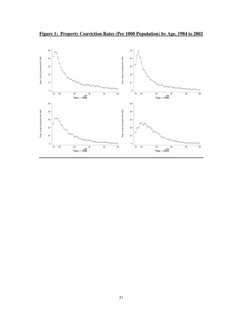
Figure 1 presents the age distribution of property crime convictions per 1000

population, for the selection of years (1984, 1990, 1996, 2002). This “age-offences

curve” shows peaks for the age group 16 to 20 and after that a strong tendency to

decrease with age. Additionally, peaks seem to be lower in 1996 and 2002 as compared

to 1984 and 1990. This is interesting for our empirical analysis since educational

attainment rises over time.

This high-to-low pattern of the age-offences curve is well supported by the

underlying theory. The combination of factors mentioned earlier (absence from school,

peer pressure, lack of parental guidance, pleasure from committing a crime, etc.),

together with the fact that young people tend to be protected from harsh punishment in

the criminal justice system, bring about high levels of youth delinquency and criminal

activity. As young people grow older, they begin to be influenced by a series of factors

which discourage them from breaking the law. As they become more independent, enter

the labour market, form their own families, and become part of their own communities,

young people begin to develop ties to society and attachments to social institutions and

norms. These factors, coupled with the possibility of more severe legal sanctions, all

encourage a lower crime rate, as young people move towards adulthood (Hansen, 2003).

Table 1 presents estimation results for different specifications of property crime

offending equations, using both the OLS and 2SLS estimating approaches. The upper

panel of the Table 1 shows six estimates of the link between property crime convictions

and average years of education, three estimated by OLS and three by 2SLS. The

specifications differ in whether or not they include LFS and NES control variables, so

columns (1) and (2) do not, columns (3) and (4) include LFS controls only (detailed in

the notes to the Table) and columns (5) and (6) include LFS controls and the NES hourly

13

wage. The lower panel of the Table shows the first stage years of education equations (for

the 2SLS models in columns (2), (4) and (6)).

Considering first the years of education equations in the lower panel of the Table,

it is clear that the first stage is strong, with the instruments being strongly significant (as

shown by the F-tests of their marginal significance). For the SLA1 variable the affected

cohort has somewhere between .47 and .50 years more schooling than an unaffected

cohort and for the SLA2 variable the comparable numbers are slightly higher at .57 to .63

years more education. These estimates clearly show that changes in the compulsory

school leaving laws significantly raised the affected cohorts’ average years of education.

In the upper panel, the estimated effect of years of education on the rates of

offending for property crimes are all estimated to be negative and, with the exception of

the column (1) model, are statistically significant. The OLS estimates, in the odd

numbered columns, vary from around –.05 to –.21, suggesting a 10% increase in the

years of schooling lowers property crime convictions by .5 to 2%. The 2SLS estimates

are bigger (in absolute terms), and lie between -0.60 and –0.77, corresponding to much

bigger effects (i.e. a 10% increase in years of schooling lowers crime by 6 to 7.7%).

Bearing in mind that a 10% increase in schooling is just over one year, these effects are

sizable.

In Table 2 we consider what is probably a more appropriate education variable,

given the nature of the instruments, the proportion of the cohort with no educational

qualifications. The table structure is the same as for Table 1, with the same six

specifications reported in the upper panel, and the first stages given in the lower panel of

the Table. Again the first stage works well, with the SLA1 group having a no

qualifications proportion around .06 to .10 lower, and the SLA2 group having a

proportion .09 to .14 lower, depending on specification. Over the sample the mean

14

proportion with no qualifications is about .25 so these are sizable impacts. The F-tests

again show the instruments to be strongly significant in the first stage.

We tend to prefer the no qualifications specifications in the 2SLS setting since the

2SLS estimator gives the rate of return for marginal individuals with high discount rates,

that is, those with less patience and low education. It is therefore interesting that, in the

case of this education variable, the OLS and 2SLS estimates in the upper panel of the

Table are much more similar to one another. The magnitudes remain large, but also seem

more plausible. According to the OLS specifications, a 10 percent increase in no

qualifications corresponds to a 31 to 40 percent higher conviction rate. In the 2SLS

specifications, comparable numbers are between 28 percent in the fully specified model

(column (6)) and 32 percent for the model with only age and year dummies (column (1)).

It is interesting that this variable is probably more appropriate than the years of

education variable in the IV context. As we have already mentioned, this is since the

local variation induced by the instrument is much more likely to have an impact at the

bottom of the education distribution and no impact at the top since people near the top

would have stayed on after the compulsory school leaving age anyway and so the change

would not affect them. For these results, the OLS and IV estimates are much more in line

with one another and suggest a strong causal link between lack of education

qualifications and property crime offending.

Table 3 examines the effect of education on convictions for property crimes for

the cohort panel of men only. The OLS and 2SLS show the latter to be larger (in absolute

terms) for both education variables, although they are in the same ballpark in terms of

magnitudes. In the OLS model (column (1)) an additional year of schooling decreases

property crime conviction rates by about 26 percent, whereas, for the 2SLS model

(column (2)), this number is rather large at 45 percent. On the other hand, a 10 percent

15

increase in no qualifications means a 26 percent higher (OLS model, column (3)) or 35

percent higher (2SLS model, column (4)) conviction rates.

So far we have considered only property crime convictions. In Table 4 we look at

convictions for violent crimes, again amongst males. These results are much less clear

regarding the impact of education on crime. In fact violent crimes, if anything, are

positively related to education (this is true in the 2SLS models, but effects are estimated

to be insignificantly different from zero in the OLS models). As violent crimes do not

respond to economic incentives in the same way as property crimes, these results would

need to be interpreted from a different perspective, not advocated in this paper.

The final set of cohort results we consider are some robustness checks, given in

Table 5. Here we present results for two specific age sub-sets, again for men. First, in

columns (1) and (2) we look at cohorts of men aged 21-59, dropping younger cohorts

who have not completed their education. Of course, this matters much more for the years

of schooling measure and so it is perhaps not surprising that the estimated effects for the

no qualifications variable are not much affected. Finally, we look at the age 21-40 cohorts

(in columns (3) and (4)), again finding the main results to be highly robust. From this we

conclude that our OID cohort analysis uncovers an important causal link between

possessing no educational qualifications and the probability of committing property crime

offences.

Approach 2

Evidence from the Offenders Index data is consistent with the hypothesis that

higher education levels reduce convictions for engaging in criminal activity. We

corroborate these findings using Census 2001 data. One limitation of the Census data is

that they do not differentiate among different types of criminal offences, since we only

know if people are imprisoned at the time the Census is taken. The second limitation is

16

that we cannot implement the 2SLS approach since we only have a single cross-section

and, once the full set of age cohort dummies is included in the estimating equation, the

instrumental variables are invalid. Instead, we perform the logit estimation approach of

the effect of schooling on incarceration rates.

Table 6 presents summary statistics for imprisonment rates, for both men and

women, by different age groups. Overall, 0.13 percent of the 16-64 year olds in the

British population were in prison, according to the 2001 Census. Imprisonment rates for

young men aged 16 to 20 are higher than average at 0.34 percent, and reach their highest

at 0.57 percent among the age 21 to 25 males. The imprisonment rates then declines for

older age groups. This is in line with the postulations of the “crime-age curve” that we

saw earlier, when using the Offenders Index data. Far fewer women are in prison and

even amongst the highest sub-group (again aged 21-25) imprisonment rates remain low.

The rest of the Table 6 shows stark differences by education. Table 6 also

presents the gap in imprisonment rates between those with no and some qualification.

Amongst some of the no qualification groups, the percent in prison rises sharply. For

example, 2.57 percent of men aged 21-25 with no educational qualifications are in prison

in 2001. The last two columns of the Table show imprisonment gaps between the no

qualification and some qualification groups. The gaps are reported in two ways, as

percentage gaps and as relative risks. It is evident that there are large gaps in

imprisonment rates that are related to the possession of educational qualifications.

Moreover, the gaps are at their largest for the age groups where more people are in

prison: see the largest relative risk ratios in the final column for the age 21-25 group, for

both men and women.13

13 For more about education and its association with the crime-age profiles see Hansen (2003).

17

Table 7 presents logit estimates that condition upon an additional range of

variables from the Census (listed in the Table). Two sets of specifications are reported for

the whole sample size, men and women separately, and for the different age by gender

groups. The two specifications differ in the way in which they specify the age control

variable – in column (1) it is entered as a quadratic, in column (2) a full set of age

dummies is included.

The results in Table 7 confirm the descriptive analysis. Even after conditioning on

a range of factors, there is a sizable gap in imprisonment rates between those with no

qualifications and those with some educational qualifications. For the full sample, the

RRR of around 4 shows that people with no qualifications are four times more likely to

be in prison than those with some qualifications. For young men these odds rise even

more, to around 9.1 for 16-20 year olds, and to 14.8 for women in the same age group.14

6. Conclusions

Education can affect the likelihood of offending in a variety of ways. In many

theoretical approaches more education leads causally to lower crime. For example,

amongst young people staying at school rather than on the streets may well influence

their choice of peers and enforce some level of discipline upon them. More generally,

education encourages people to develop skills and acquire knowledge and training that

affects their future life chances, like acquiring legally paid jobs with satisfactory wages.

14 The Census education variable is more detailed than the no/some educational qualifications split we consider. There is information on five qualification levels, ranging from Level 0 (No Qualifications) through to Level 4 (Degree or higher). We look at the no/some distinction so we can include the young people in our sample since some may not have completed their education, and these are an important group to consider in studies of criminal activity. Specifications estimated for older samples that enter in four dummy variables for No Qualifications, Level 1, Level 2 and Level 3 (omitting Level 4 as the reference category) show a monotonic relationship between the probability of imprisonment and qualification attainment. For example, for men aged 26-30 the relative risk ratios were estimated as 13.46 (Level 0), 6.32 (Level 1), 5.56 (Level 2), 2.27 (Level 3).

18

This paper presents some new evidence on the effect of education on crime,

looking at two different data sources from Britain. In the first, property crime convictions

in England and Wales (taken from using unique Home Office Offenders Index data

matched to household and employer surveys) are seen to be significantly lower amongst

age cohorts where education is higher. To ensure the direction of causation runs from

education to crime (and not in the opposite direction), we follow the idea of Lochner and

Moretti (2004) and use exogenous changes in school leaving age laws as instruments for

our education variable. Two stage least squares estimates based on this approach show

that education significantly reduces property crime convictions. Our second approach,

based on using 2001 Census data on imprisonment and educational qualifications,

corroborate these finding by demonstrating that having no educational qualifications

significantly increases the risk of imprisonment.

As always there is a range of possible extensions of this work. For example,

further analysis could usefully break down among different types of crime in more detail,

examine factors that affect the crime-age profiles of those with some and no educational

qualifications, and try to estimate social savings from crime reduction.

There is little doubt that findings from this paper have important implications for

longer-term efforts aimed at reducing crime. It is evident that crime is a negative

externality with enormous social costs. If education reduces crime, then schooling will

have social benefits that are not taken into account by individuals. In this case, the social

returns to education may exceed the private return. Hence, policymakers should continue

to devote attention towards the design of social and educational policies that can have an

impact on the crime-education nexus.

19

References

Calvó-Armengol, A. and Y. Zenou (2004), “Social Networks and Crime Decision: The

Role of Social Structure in Facilitating Delinquent Behaviour,” International

Economic Review, 45, 939-958.

Case, A. C. and L. F. Katz (1991), “The Company You Keep: The Effects of Family and

Neighbourhood Disadvantaged Youths,” NBER Working Paper, No. 3705.

Ehrlich, I. (1975), “On the Relation between Education and Crime,” In F. T. Juster,

editor, Education, Income, and Human Behaviour, chapter 12, McGraw-Hill Book

Co., New York.

Farrington, D. P. (2001), “Predicting Persistent Young Offenders,” in G. L. McDowell

and J. S. Smith, editors, Juvenile Delinquency in the US and the UK, Macmillan

Press Ltd., United Kingdom.

Farrington, D. P., G. C. Barnes and S. Lambert (1996), “The Concentration of Offending

in Families,” Legal and Criminological Psychology, 1, 47-63.

Feinstein, L. (2002), “Quantitative Estimates of the Social Benefits of Learning, 1:

Crime,” Wider Benefits of Learning Research Report, No. 5.

Feinstein, L. and R. Sabates (2005), “Education and Youth Crime: Effects of Introducing

the Education Maintenance Allowance Programme,” Wider Benefits of Learning

Research Report, No. 14.

Gould, D., D. Mustard and B. Weinberg (2002), “Crime Rates and Local Labor Market

Opportunities in the United States: 1979-1997”, Review of Economics and Statistics,

84, 45-61.

Grogger, J. (1998), “Market Wages and Youth Crime,” Journal of Labour Economics, 16,

756-791.

Hansen, K. (2003), “Education and the Crime-Age Profile,” British Journal of

Criminology, 43, 141-168.

Harmon, C. and I. Walker (1995), “Estimates of the Economic Return to Schooling for

the United Kingdom,” American Economic Review, 85, 1278-1286.

Hirschi, T. and M. Gottfredson (1995), “Control Theory and the Life-Course

Perspective,” Studies on Crime Prevention, 4, 131-142.

Labour Force Survey User Guide (2003), Volume 1: Background and Methodology;

Volume 3: Details of LFS Variables.

20

Levitt, S. D. and L. Lochner (2001), "The determinants of juvenile crime," in J. Gruber,

Risky Behaviour Among Youths: An Economic Analysis, Chicago, IL: University of

Chicago Press, pp. 327-73.

Lochner, L. (2004), “Education, Work, and Crime: A Human Capital Approach,”

International Economic Review, 45, 811-843.

Lochner, L. and E. Moretti (2004), “The Effect of Education on Crime: Evidence from

Prison Inmates, Arrests, and Self-Reports,” American Economic Review, 94, 155-

189.

Ludwig, J., G.J. Duncan and P. Hirschfield (2001), “Urban Poverty and Juvenile Crime:

Evidence from a Randomized Housing-Mobility Experiment,” Quarterly Journal of

Economics, 116, 655-679.

Machin, S. and C. Meghir (2004), “Crime and Economic Incentives,” Journal of Human

Resources, 39, 958-79.

Offenders Index (1998a), “Codebook,” Research Development and Statistics Directorate,

Home Office.

Offenders Index (1998b) “A User’s Guide,” Research Development and Statistics

Directorate, Home Office.

Rutter, M., H. Giller and A. Hagell (1998), “Antisocial Behaviour by Young People,”

Cambridge University Press, Cambridge.

Soothill, K., B. Francis, B. Sanderson and E. Ackerley (2000), “Sex Offenders:

Specialists, Generalists – or Both,” British Journal of Criminology, 40, 56-67.

Tauschen, H., A. D. Witte and H. Griesinger (1994), “Criminal Deterrence: Revisiting

the Issue With a Birth Cohort”, Review of Economics and Statistics, 76, 399-412.

21

Figure 1: Property Conviction Rates (Per 1000 Population) by Age, 1984 to 2002

Pro

p. C

rime

Con

vict

ions

Per

100

0

Year = 1984age

16 20 30 40 50 59

0

.01

.02

.03

.04

.05

Pro

p. C

rime

Con

vict

ions

Per

100

0

Year = 1990age

16 20 30 40 50 59

0

.01

.02

.03

.04

.05

Pro

p. C

rime

Con

vict

ions

Per

100

0

Year = 1996age

16 20 30 40 50 59

0

.01

.02

.03

.04

.05

Pro

p. C

rime

Con

vict

ions

Per

100

0

Year = 2002age

16 20 30 40 50 59

0

.01

.02

.03

.04

.05

22

Table 1: Property Crime Convictions and Years of Education

Log(Property Crime Convictions Per 1000 Population), by Age and Year, 16-59 Year Olds, 1984-2002

A. Crime Equations (1) (2) (3) (4) (5) (6) OLS 2SLS OLS 2SLS OLS 2SLS Years of Education -.053

(.055) -.773 (.124)

-.149 (.054)

-.667 (.106)

-.214 (.050)

-.599 (.093)

Age Dummies (43) Yes Yes Yes Yes Yes Yes Year Dummies (19) Yes Yes Yes Yes Yes Yes LFS Control Variables No No Yes Yes Yes Yes NES Hourly Wage No No No No Yes Yes Sample Size 836 836 836 836 792 792 B. First Stage Years of Education Equations SLA1 - .465

(.031) - .498

(.028) - .493

(.027) SLA2 - .626

(.040) - .568

(.036) - .577

(.035) Age Dummies (43) - Yes - Yes - Yes Year Dummies (19) - Yes - Yes - Yes LFS Control Variables - No - Yes - Yes NES Hourly Wage - No - No - Yes F-Test of Significance of SLA1 and SLA2 (P-Value)

- F(2, 772) = 125.6

(P = .000)

- F(2, 767) = 159.7

(P = .000)

- F(2, 723) = 168.0

(P = .000) Sample Size - 836 - 836 - 792

Notes: Models estimated on age-year cells, for 16-59 year olds between 1984 and 2002. Standard errors in parentheses. The LFS control variables are: proportion male, proportion employed, proportion non-white, proportion of employed in full-time jobs, proportion living in London. SLA1 = 1 for those with compulsory school leaving age of 15 (raised from 14 in 1947), = 0 otherwise; SLA2 = 1 for those whose with compulsory school leaving age of 16 (raised from 15 in 1973), = 0 otherwise. The specifications including the NES hourly wage are estimated up to 2001 only.

23

Table 2: Property Crime Convictions and No Educational Qualifications

Log(Property Crime Convictions Per 1000 Population), by Age and Year, 16-59 Year Olds, 1984-2002

A. Crime Equations (1) (2) (3) (4) (5) (6) OLS 2SLS OLS 2SLS OLS 2SLS No Qualifications 3.113

(.195) 3.194 (.435)

3.954 (.233)

2.577 (.570)

3.313 (.259)

2.767 (.585)

Age Dummies (43) Yes Yes Yes Yes Yes Yes Year Dummies (19) Yes Yes Yes Yes Yes Yes LFS Control Variables No No Yes Yes Yes Yes NES Hourly Wage No No No No Yes Yes Sample Size 836 836 836 836 792 792 B. First Stage No Qualification Equations SLA1 - -.102

(.008) - -.068

(.006) - -.062

(.005) SLA2 - -.141

(.010) - -.098

(.008) - -.089

(.007) Age Dummies (43) - Yes - Yes - Yes Year Dummies (19) - Yes - Yes - Yes LFS Control Variables - No - Yes - Yes NES Hourly Wage - No - No - Yes F-Test of Significance of SLA1 and SLA2 (P-Value)

- F(2, 772) = 96.8

(P = .000)

- F(2, 767) = 81.5

(P = .000)

- F(2, 723) = 89.1

(P = .000) Sample Size - 836 - 836 - 792

Notes: Models estimated on age-year cells, for 16-59 year olds between 1984 and 2002. Standard errors in parentheses. The LFS control variables are: proportion male, proportion employed, proportion non-white, proportion of employed in full-time jobs, proportion living in London. SLA1 = 1 for those with compulsory school leaving age of 15 (raised from 14 in 1947), = 0 otherwise; SLA2 = 1 for those whose with compulsory school leaving age of 16 (raised from 15 in 1973), = 0 otherwise. The specifications including the NES hourly wage are estimated up to 2001 only.

24

Table 3: Property Crime Convictions and No Educational Qualifications, Males Separately

Log(Property Crime Convictions Per 1000 Population),

by Age and Year, 16-59 Year Olds, 1984-2001, Males Males A. Crime Equations (1) (2) (3) (4) OLS 2SLS OLS 2SLS Years of Education -.259

(.048) -.451 (.094)

- -

No Qualifications - - 2.571 (.224)

3.483 (.564)

Age Dummies (43) Yes Yes Yes Yes Year Dummies (19) Yes Yes Yes Yes LFS Control Variables Yes Yes Yes Yes NES Hourly Wage Yes Yes Yes Yes Sample Size 792 792 792 792 B. First Stage Equations SLA1 - .524

(.032) - -.080

(.007) SLA2 - .570

(.041) - -.076

(.009) Age Dummies (48) - Yes - Yes Year Dummies (19) - Yes - Yes LFS Control Variables - Yes - Yes NES Hourly Wage - Yes - Yes F-Test of Significance of SLA1 and SLA2 (P-Value)

- F(2, 724) = 133.0

(P = .000)

- F(2, 724) = 69.5

(P = .000) Sample Size - 792 - 792

Notes: Models estimated on age-year cells, for 16-59 year olds between 1984 and 2001. Standard errors in parentheses. The LFS control variables are: proportion male, proportion employed, proportion non-white, proportion of employed in full-time jobs, proportion living in London. SLA1 = 1 for those with compulsory school leaving age of 15 (raised from 14 in 1947), = 0 otherwise; SLA2 = 1 for those whose with compulsory school leaving age of 16 (raised from 15 in 1973), = 0 otherwise.

25

Table 4: Violent Crime Convictions and No Educational Qualifications, Males Separately

Log(Violent Crime Convictions Per 1000 Population), by Age and Year, 16-59 Year Olds, 1984-2001, Males

Males A. Crime Equations (1) (2) (3) (4) OLS 2SLS OLS 2SLS Years of Education .036

(.066) .307

(.130) - -

No Qualifications - - -.494 (.330)

-1.210 (.824)

Age Dummies (43) Yes Yes Yes Yes Year Dummies (19) Yes Yes Yes Yes LFS Control Variables Yes Yes Yes Yes NES Hourly Wage Yes Yes Yes Yes Sample Size 792 792 792 792 B. First Stage Equations SLA1 - .524

(.032) - -.080

(.007) SLA2 - .570

(.041) - -.076

(.009) Age Dummies (43) - Yes - Yes Year Dummies (19) - Yes - Yes LFS Control Variables - Yes - Yes NES Hourly Wage - Yes - Yes F-Test of Significance of SLA1 and SLA2 (P-Value)

- F(2, 724) = 133.0

(P = .000)

- F(2, 724) = 69.5

(P = .000) Sample Size - 792 - 792

Notes: Models estimated on age-year cells, for 16-59 year olds between 1984 and 2001. Standard errors in parentheses. The LFS control variables are: proportion male, proportion employed, proportion non-white, proportion of employed in full-time jobs, proportion living in London. SLA1 = 1 for those with compulsory school leaving age of 15 (raised from 14 in 1947), = 0 otherwise; SLA2 = 1 for those whose with compulsory school leaving age of 16 (raised from 15 in 1973), = 0 otherwise.

26

Table 5: Checks of Robustness

Log(Property Crime Convictions Per 1000 Population), by Age and Year, 1984-2001, Males

Ages 21-59 Ages 21-40 A. Crime Equations (1) (2) (3) (4) OLS 2SLS OLS 2SLS No Qualifications 2.643

(.270) 3.019 (.794)

2.276 (.292)

3.471 (.800)

Age Dummies (38/19) Yes (38) Yes (38) Yes (19) Yes (19) Year Dummies (19) Yes Yes Yes Yes LFS Control Variables Yes Yes Yes Yes NES Hourly Wage Yes Yes Yes Yes Sample Size 702 702 360 360 B. First Stage No Qualification Equations SLA1 - -.064

(.007) - -

SLA2 - -.061 (.009)

- -.031 (.004)

Age Dummies (38/19) - Yes (38) - Yes (19) Year Dummies (19) - Yes - Yes LFS Control Variables - Yes - Yes NES Hourly Wage - Yes - Yes F-Test of Significance of SLA1 and SLA2 (P-Value)

- F(2, 639) = 41.8

(P = .000)

- F(1, 317) = 52.0

(P = .000) Sample Size - 702 - 360

Notes: Models estimated on age-year cells, for 16-59 year olds between 1984 and 2001. Standard errors in parentheses. The LFS control variables are: proportion male, proportion employed, proportion non-white, proportion of employed in full-time jobs, proportion living in London. SLA1 = 1 for those with compulsory school leaving age of 15 (raised from 14 in 1947), = 0 otherwise; SLA2 = 1 for those whose with compulsory school leaving age of 16 (raised from 15 in 1973), = 0 otherwise.

27

Table 6: Imprisonment Rates (Percent), 2001 Census

All No Educational Qualifications

Some Educational Qualifications

Imprisonment Rate

Number of

People

Imprisonment Rate

Number of

People

Imprisonment Rate

Number of

People

Gap in Imprisonment

Rate Between No

and Some Qualifications

(Standard error)

Relative Risk Ratio

All 0.13 1099639 0.23 294871 0.09 804768 0.14 (0.01) 2.58 Men 0.25 535820 0.44 142373 0.17 393447 0.27 (0.02) 2.61 Men, Aged 16-20

0.34 57418 0.91 12048 0.18 45370 0.73 (0.06) 5.03

Men, Aged 21-25

0.57 52889 2.57 6176 0.30 46713 2.27 (0.10) 8.67

Men, Aged 26-30

0.42 58977 1.41 8036 0.27 50941 1.14 (0.08) 5.37

Men, Aged 31-64

0.16 366536 0.22 116113 0.13 250423 0.09 (0.01) 1.74

Women 0.01 563819 0.03 152498 0.01 411321 0.02 (0.003) 2.70 Women, Aged 16-20

0.01 54934 0.05 9856 0.01 45078 0.04 (0.01) 7.62

Women, Aged 21-25

0.04 53852 0.17 5229 0.02 48623 0.15 (0.03) 8.38

Women, Aged 26-30

0.02 62415 0.07 7153 0.01 55262 0.06 (0.02) 4.83

Women, Aged 31-64

0.01 392618 0.02 130260 0.01 262358 0.01 (0.003) 2.22

Notes: Based on 16-64 year olds in the 3% Census microdata sample.

28

Table 7: Logit Estimates of Imprisonment Equations

Specification 1:

Includes quadratic in age, 15 country of birth dummies, gender dummy

(where applicable), non-white dummy, 5 marital status dummies,

dummy for never worked, dummies for country

Specification 2: Includes age dummies, 15 country of

birth dummies, gender dummy (where applicable), non-white

dummy, 5 marital status dummies, dummy for never worked, dummies

for country Coefficient on

No Qualifications

Dummy Variable (standard error in round brackets,

marginal effect X 100 in square

brackets)

Sample Size Coefficient No

Qualifications Dummy Variable (standard error in round brackets,

marginal effect X 100 in square

brackets)

Sample Size

All 1.389 (0.058) [0.18]

RRR = 4.01

1099639 1.417 (0.058) [0.18]

RRR = 4.12

1099639

Men 1.385 (0.060) [0.34]

RRR = 4.00

535820 1.412 (0.060) [0.35]

RRR = 4.11

535820

Men, Aged 16-20 2.209 (0.152) [0.74]

RRR = 9.11

57418 2.210 (0.152) [0.74]

RRR = 9.11

57418

Men, Aged 21-25 2.011 (0.122) [1.14]

RRR = 7.47

52889 2.011 (0.122) [1.14]

RRR = 7.47

52889

Men, Aged 26-30 1.302 (0.143) [0.54]

RRR = 3.67

58977 1.301 (0.144) [0.54]

RRR = 3.67

58977

Men, Aged 31-64 0.716 (0.092) [0.11]

RRR = 2.05

366536 0.717 (0.092) [0.11]

RRR = 2.05

366536

Women 1.464 (0.254) [0.02]

RRR = 4.32

563819 1.498 (0.254) [0.02]

RRR = 4.47

563819

Women, Aged 16-20 2.694 (0.755) [0.04]

RRR = 14.79

54934 2.697 (0.754) [0.04]

RRR = 14.84

54934

Women, Aged 21-25 2.095 (0.510) [0.07]

RRR = 8.12

53852 2.097 (0.510) [0.07]

RRR = 8.14

53852

Women, Aged 26-30 0.886 (0.697) [0.02]

RRR = 2.42

62415 0.878 (0.699) [0.02]

RRR = 2.41

62415

Women, Aged 31-64 1.150 (0.346) [0.01]

RRR = 3.16

392618 1.157 (0.346) [0.01]

RRR = 3.18

392618

29

Appendix

Table A1: Type of Communal Establishment, England, Wales and Scotland,

Census 2001

Value Label Percentage

-9 Not Applicable 98.3

1 NHS psychiatric hospital 0.0

2 Other NHS hospital/home 0.1

3 LA Children’s home 0.0

4 LA Nursing home 0.0

5 LA Residential care home 0.1

6 LA Other home 0.0

7 HA home or hostel 0.0

8 Nursing homes (not HA/LA) 0.3

9 Residential home (not HA/LA) 0.4

10 Children’s home (not HA/LA) 0.0

11 Psychiatric hospital (not HA/LA) 0.0

12 Other hospital (not HA/LA) 0.0

13 Other medical and care home (not HA/LA) 0.0

14 Defence establishment (inc. ships) 0.1

15 Prison service establishment 0.1

16 Probation/bail hostel (not Scotland) 0.0

17 Educational establishment 0.5

18 Hotel/boarding house, guest home 0.1

19 Hostel (inc. youth hostel, hostels for homeless and persons sleeping rough) 0.1

20 Civilian ship, boat or barge 0.0

21 Other 0.1

Source: 2001 Individual CAMS Codebook, http://www.ccsr.ac.uk/sars