Credit Supply Responses to Reserve Requirement: loan … · Credit Supply Responses to Reserve Requirement: loan-level evidence from macroprudential policye Requirement: loan-level

Credit Supply Responses to Reserve Requirement: loan-level evidence from macroprudential policye

Requirement: loan-level evidence from macroprudential policy

João Barata R. B. Barroso, Rodrigo Barbone Gonzalez and Bernardus F. Nazar Van Doornik

November 2017

467

ISSN 1518-3548 CGC 00.038.166/0001-05

Working Paper Series Brasília no. 467 NNovemberember

2017 p. 1-42

Working Paper Series

Edited by the Research Department (Depep) – E-mail: [email protected]

Editor: Francisco Marcos Rodrigues Figueiredo – E-mail: [email protected]

Co-editor: José Valentim Machado Vicente – E-mail: [email protected]

Editorial Assistant: Jane Sofia Moita – E-mail: [email protected]

Head of the Research Department: André Minella – E-mail: [email protected]

The Banco Central do Brasil Working Papers are all evaluated in double-blind refereeing process.

Reproduction is permitted only if source is stated as follows: Working Paper no. 467.

Authorized by Carlos Viana de Carvalho, Deputy Governor for Economic Policy.

General Control of Publications

Banco Central do Brasil

Comun/Divip

SBS – Quadra 3 – Bloco B – Edifício-Sede – 2º subsolo

Caixa Postal 8.670

70074-900 Brasília – DF – Brazil

Phones: +55 (61) 3414-3710 and 3414-3565

Fax: +55 (61) 3414-1898

E-mail: [email protected]

The views expressed in this work are those of the authors and do not necessarily reflect those of the Banco Central do

Brasil or its members.

Although the working papers often represent preliminary work, citation of source is required when used or reproduced.

As opiniões expressas neste trabalho são exclusivamente do(s) autor(es) e não refletem, necessariamente, a visão do Banco Central do Brasil.

Ainda que este artigo represente trabalho preliminar, é requerida a citação da fonte, mesmo quando reproduzido parcialmente.

Citizen Service Division

Banco Central do Brasil

Deati/Diate

SBS – Quadra 3 – Bloco B – Edifício-Sede – 2º subsolo

70074-900 Brasília – DF – Brazil

Toll Free: 0800 9792345

Fax: +55 (61) 3414-2553

Internet: http//www.bcb.gov.br/?CONTACTUS

Non-technical Summary

This paper estimates the impact of reserve requirements (RR) on the credit

supply in Brazil. We use a database that covers virtually all loans to private non-

financial firms. The period considered is from 2008Q1 to 2015Q2. During this period,

there were several interventions using RR. In our first exercise, we average RR shocks

using a macroprudential policy index. In a second exercise, we focus on credit supply

responses from a countercyclical easing policy in the aftermath of the 2008 global crisis

and from its related tightening.

RR operate directly on the supply reaction of bank credit to a change in funding

composition. This reaction may depend on the state of the economy and on bank

characteristics. It also has implications on the composition of credit along the riskiness

of borrowers. Estimates of the effects of RR on the credit supply are important for

emerging markets. Particularly for countries that use RR to smooth the credit cycle.

However, with one exception, there is no loan-level evidence of the impact of RR. We

contribute to this literature by exploring a larger and longer dataset with policy shocks

from tightening and easing cycles.

The results from the first exercise show that a RR easing increases credit by

treated banks relative to non-treated banks. A tightening of RR has the opposite effect.

From the second exercise, we find that the tightening phase of RR affected the lending

channel on average less than the easing one. This suggests that the supply of bank credit

is more reactive to an easing than to a tightening. We find evidence that small and

foreign banks mitigate this channel. Finally, banks are prone to lend less to riskier firms

during easing and to riskier firms during tightening.

3

Sumário Não-Técnico

O artigo estima o impacto sobre a oferta de crédito de mudanças nas alíquotas de

recolhimento compulsório brasileiras. Os dados cobrem essencialmente todos os

empréstimos concedidos a firmas não-financeiras de controle privado, do primeiro

trimestre de 2008 ao segundo trimestre de 2015. Durante este período, várias alterações

nos recolhimentos compulsórios foram implementadas. Em um primeiro exercício, os

choques sobre os compulsórios são suavizados através de um índice de medidas

macroprudenciais. Em um segundo exercício, estudamos a resposta da oferta de crédito

a uma redução nos níveis do compulsório em 2008, implementada em resposta a crise

de crédito global; e, posteriormente, de seu aumento em 2010, já num contexto de

recuperação dos mercados de crédito no Brasil.

A reação às mudanças nos recolhimentos compulsórios pode depender do estado

da economia e das características dos bancos. Ela também tem implicações para a

composição e o risco de crédito dos tomadores de empréstimos. As estimativas dos

efeitos do compulsório sobre a oferta de crédito são relevantes para mercados

emergentes, principalmente para aqueles que utilizam essa ferramenta para suavizar o

ciclo de crédito. Contudo, há pouca evidência, em nível dos empréstimos, para o

impacto destas medidas, e nenhuma utilizando uma base tão extensa e cobrindo tantos

períodos, incluindo ciclos de aperto e de afrouxamento nas alíquotas dos recolhimentos

compulsórios.

Os resultados do primeiro exercício mostram que um aumento de liquidez com

relaxamento dos recolhimentos compulsórios aumenta a concessão de créditos nos

bancos afetados por esta redução. Uma redução na liquidez através do aperto nos

recolhimentos compulsórios tem o efeito contrário. Os resultados do segundo exercício

mostram que a fase de aperto dos recolhimentos compulsórios teve menos impacto

sobre os empréstimos do que a fase de relaxamento, o que sugere que a oferta de crédito

bancário reage mais a este último tipo de choque. Também há evidência de que tais

políticas têm menos efeito em bancos pequenos e em bancos estrangeiros. Finalmente,

bancos tendem a emprestar mais para firmas mais arriscadas em um período de

relaxamento, e menos para as firmas mais arriscadas durante um aperto de liquidez

obtido com o aumento das alíquotas de compulsório.

4

Credit Supply Responses to Reserve Requirement:

loan-level evidence from macroprudential policy *

João Barata R. B. Barroso†

Rodrigo Barbone Gonzalez‡

Bernardus F. Nazar Van Doornik§

Abstract

This paper estimates the impact of reserve requirements (RR) on credit

supply in Brazil, exploring a large dataset with several policy shocks. We

use a difference-in-difference strategy; first in a long panel, then in a cross-

section exploring the effects of changes in RR on credit. In the first case, we

average several RR changes from 2008 to 2015 using a macroprudential

policy index. In the second, we use the bank-specific regulatory change to

estimate credit supply responses from (1) a countercyclical easing policy

implemented to alleviate a credit crunch in the aftermath of the 2008 global

crisis; and (2) from its related tightening. We find evidence of a lending

channel where more liquid banks mitigate RR policy. Exploring the two

phases of countercyclical policy, we find that the easing impacted the

lending channel on average two times more than the tightening. Foreign and

small banks mitigate theses effects.

Keywords: Reserve requirement, credit supply, capital ratio, liquidity ratio,

macroprudential policy.

JEL Codes: E51, E52, E58, G21, G28

The Working Papers should not be reported as representing the views of the Banco Central

do Brasil. The views expressed in the papers are those of the author(s) and do not

necessarily reflect those of the Banco Central do Brasil.

________________________ *Paper produced as part of the BIS Consultative Council for the Americas (CCA) research project on

"The impact of macroprudential policies: an empirical analysis using credit registry data" implemented by

a Working Group of the CCA Consultative Group of Directors of Financial Stability (CGDFS). We are

grateful to seminar participants at the 2016 BIS Meeting in Mexico, and at the XI Seminário de Riscos e

Estabilidade Financeira in Sao Paulo (Brazil) for many helpful comments and suggestions. Additionally,

we would like to thank the Department of Banking Operations and Payment System of the Central Bank

of Brazil for providing us with data and permanent support on reserve requirements. We also appreciate

the help of Carlos Leonardo Kulnig Cinelli. † Banco Central do Brasil, Research Department: [email protected]. ‡ Banco Central do Brasil, Research Department: [email protected] § Banco Central do Brasil, Research Department: [email protected].

5

http://www.bis.org/am_office/wgfinstab/teompatiwmp.htm

mailto:[email protected]

mailto:[email protected]

1. Introduction

Reserve requirements (RR) operate directly on the narrow credit channel defined

by the supply reaction of bank credit to a change in funding composition (Calomiris and

Khan, 1991, Stein, 1998, Diamond and Rajan, 2011, Calomiris et al., 2015). This

reaction may depend on the state of the macroeconomy, and on bank characteristics,

such as liquidity or capital (Kashyap and Stein (2000), Holmstrom and Tirole (1997),

Mora (2014)). It has also implications for the composition of credit along the riskiness

of the borrowers (Camors et al. (2016)). In this paper, we estimate the impact of RR on

credit supply in Brazil.

Quantitative estimates of the effect of RR in the supply of credit, as well as its

complementarity or substitution relations with other variables, are important for

emerging markets that traditionally use RR policy to smooth the credit cycle (Montoro

and Moreno (2011), Cordella et al. (2014)). Yet, with the exception of Camors et al.

(2016), there is no loan-level evidence of the impact of such policies in these markets.

We build on their work, but exploring a larger and longer dataset with policy shocks

from tightening and loosening cycles. Additionally, we provide an analysis using a long

panel to capture macroeconomic and bank heterogeneity effects on the composition of

the policy shocks.

We use quarterly data from 2008Q1 to 2015Q2 from “Sistema de Informações

de Crédito” (SCR), Central Bank of Brazil (BCB) credit registry dataset covering

virtually all loans to private non-financial firms1. During this time span, BCB made

several macroprudential interventions using RR including a major countercyclical one

in the aftermath of the global crisis. The intervention consisted of: (1) an easing, i.e.

releasing RR in November 2008 in response to a credit crunch following the global

1 Up to December 2011 it covered all loans greater than BRL 5,000 (USD 3,000 in 2011), and, after that,

all loans greater than BRL 1,000 (USD 425 in 2014).

6

financial crisis; and (2) a tightening, i.e. reversing the easing policy on March 2010,

when credit growth was overheated.

BCB made other interventions though. For instance, a tightening in December

2010, in the context of high capital inflows and credit growth2; and several easing

innovations starting with the reversal of this policy in 2012, but also along 2013 and to

2015 during an economic downturn. Before and after the policy shocks, RR ratios were

mostly flat and revolving around the long-term average of 23% of liabilities subject to

reserve requirements (LRR).

The measurement of reserve requirement innovation and sample selection is a

central piece in the identification strategy. We evaluate two broad different approaches.

In the first approach, we build an index, adding or subtracting one unit upon tightening

or easing of RR policy, respectively, and use a long panel with controls for

macroeconomic confounding factors. In the second approach, we define bank level

continuous treatment variables based on RR counterfactuals. Specifically, we define a

bank-level treatment as the excess variation in RR over the counterfactual variation one

would observe in RR under the old regulation. Notice that the counterfactual filters out

determinants of reserve requirement other than the regulatory changes. . The

counterfactuals are independently calculated to capture the regulatory changes of

November 2008 (easing - following “bad times”), and March 2010 (tightening -

following “good times”).

We identify the complementarity or substitution relations with RR policy by

introducing interaction terms in our models. We explore interactions with bank control

variables such as size, liquidity, capital ratio and risk proxies.

2 See Barroso et.al (2015) for evidence on the link between capital inflows and credit growth.

7

Following Khwaja and Mian (2008) and Jiménez et al. (2014)3, we focus on

firms with multiple bank relationships and firm (or firm*bank) fixed effects to control

for credit demand. In order to explore interactions of the treatment variable with firm or

firm-bank characteristics such as credit risk of a particular firm, we also include bank

fixed effects.

This paper contributes to the scarce literature estimating the effects of RR policy

shocks on credit supply. It also addresses synergies between macroprudential and bank

and firm heterogeneity, covering a very large dataset of firm loans. The dynamics of the

Brazilian case allows the study of both macroprudential loosening and tightening

separately.

We find in the long panel that RR policy impacts credit in the expected

direction, which is RR easing increases credit, while RR tightening decreases credit on

the treated banks relatively to the non-treated banks. The exact quantitative impact

depends on the specification, and it is sensibly higher in the long-run (one-year ahead

cumulative effect) than in the short-run (one-quarter ahead). On the countercyclical RR

policy shocks, we find that the tightening phase of countercyclical policy affected the

lending channel on average less than the easing one, suggesting that bank credit supply

is more reactive to the easing than to the tightening.

We also find bank and firm heterogeneity in the composition of these policy

events. Foreign and small banks mitigate the policy effects. On the risk-taking channel,

we find that banks more affected by countercyclical RR policy avoid riskier firms.

These results are of great concern to policymakers in charge of financial stability,

because riskier firms are the ones more affected by credit crunches and more prone to

leverage during credit booms.

3 In contrast with Jiménez el al (2014), we can study the risk-taking channel without the triple interaction

proposed in that paper. That is, the capital ratio is not a source of identification.

8

2. Literature review

The rationale for reserve requirements effects on credit supply follows Stein

(1998), and Kashyap and Stein (2000). They explore imperfect substitution between

insured and reservable bank liabilities on one side, and noninsured and non-reservable

bank liabilities on the other. The risk-taking channel on macroprudential policy follows

mostly Adrian and Shin (2009) and Dell’Ariccia et al. (2009). They show that changing

the cost of liabilities affects banks’ leverage and therefore the incentives for banks to

monitor. The interaction with banks’ liquidity and capital are presented in Kashyap and

Stein (2000), and Holmstrom and Tirole (1997), respectively.

Tovar et al. (2012), Montoro and Moreno (2011), and Bustamante and Hamman

(2015) highlight the use of reserve requirements with macroprudential purposes,

especially to foster financial stability. First, it can serve as a countercyclical tool to

manage the credit cycle in a broad context, limiting the excessive leverage of borrowers

in the upswing and operating as a liquidity buffer in the downswing. Second, it can help

to contain systemic risk accumulation by improving the liquidity of the banking system.

Third, RR can target specific sectors to ease (or impose) liquidity constraints. Fourth, it

can be a complementary tool for capital requirements.

Cerutti et al. (2015) document that macroprudential policies are more effective

and used more broadly in less developed and more closed economies, with effectiveness

measured by the correlation with credit aggregates. Cordella et al. (2014) argue that

developing countries use reserve requirements for stabilizing capital flows and the

credit cycle when there are severe limits on the typical monetary policy ability to

smooth the level of credit and/or economic activity. According to these authors, the

financial stability and business cycle-driven uses of reserve requirements cannot be

separated one from the other. When reserve requirements are used to prevent financial

9

instability, they can contribute to macroeconomic stabilization, whereas when they are

used to smooth activity, they also smooth the credit cycle and promote financial

stability.

There is a growing empirical literature exploring the risk-taking channel of

monetary policy. Jiménez et al (2014) find that banks extend more credit to riskier firms

during monetary policy easing cycles. Altumbas et.al (2012) show solvency problems

during the crisis were more severe for banks in jurisdictions with low interest rates for a

long time and for banks with less capital. Maddaloni and Peydró (2011) show a

deterioration in lending standards across several jurisdictions in response to lower short-

term interest rates. Lee et.al (2015) use syndicated loan data to show that, before the

crisis, lenders invest in riskier loans in response to a decline in short-term US rates

while, after it, in response to a decline in long-term US interest rates.

In passing, the effect of typical monetary policy on credit supply and risk taking

could be, in theory, similar to reserve requirements, although operating through other

channels. Cerutti et al. (2012) document with macro data that RR affects credit growth,

but have no implications for risk-taking. However, recent loan-level evidence from

Camors et al. (2016) and Jiménes et al. (2017) describe the opposite , suggesting a

similar bank lending channel, but one opposite and positive risk-taking channel than the

monetary policy one. The authors find a “search-for-yield” or positive risk-taking

response to the tightening of RR and countercyclical dynamic provisions respectively.

Camors et al. (2016) is the closest paper to ours in the literature. Using loan level

data and an identification strategy equal to ours, they show that an increase in RR in

Uruguay implies a contraction of credit supply. However, the macroprudential

tightening shock they explore is different in nature. While we explore countercyclical

RR policy shocks motivated by a credit crunch and later by a credit boom, the

10

tightening RR policy they explore is motivated by intense foreign cash inflows

(bypassing monetary policy). Their results for the lending channel is of similar

magnitude to ours, i.e. a RR increase of 1 percentual point (pp) translates into a credit

supply contraction of 0.66% for the most affected bank relatively to the same firm. The

authors also find that the most affected banks mitigate this tightening contracting less

credit to the riskier firms. We find a similar risk-taking channel to the easing, but not to

the tightening of RR.

3. Background

The ratio of reserve requirement to deposits in Brazil is large by international

standards. It averages 23% of total liabilities subject to RR (LRR) from 2008 to 2015,

while Montoro and Moreno (2015) report emerging market ratios below 15% and

developed market ratios below 5%. The ratio in Brazil is mostly flat before the global

financial crisis. During the crisis, in face of a liquidity squeeze in the interbank and

credit market, BCB reduces RR to the historical low levels of 18% in November 2008.

In March 2010, RR is rebuilt to its prior levels, in the first countercyclical policy use of

this kind. The easing policy was highly relevant with an immediate release of cash into

the financial system worth 3.27% of total banks´ assets (or 15% of banks’ liquid assets).

In response to an increase in capital flows and high credit growth, a major

tightening cycle starts in December 2010. Relative to other local macroprudential

policies implemented during the same period, RR is arguably the macroprudential tool

with broadest scope and biggest impact4. Along 2012, with growing external

uncertainties, reduction of international capital flows and reduced credit supply from

4 During the post-crisis environment of large global liquidity, the Central Bank of Brazil issued many

with-in sector regulations focusing on financial stability, such as loan-to-value caps on housing loans

(Araujo et al., 2016) and higher capital requirements on auto-loans (Martins and Schetchman, 2013).

However, RR is arguably the more representative measure. See Pereira da Silva and Harris (2012).

11

private banks, RR is eased again to pre-crisis levels (this latest tightening cycle is

complete). See Figures 1 and 2.

BCB manages mainly four RR components; RR on demand deposits

(unremunerated), savings (remunerated according to savings accounts), time and term

deposits (remunerated at the overnight funds rate, SELIC), and an additional component

comprised of three subcomponents, one for each of the previous components, (all

remunerated at the daily prime rate, SELIC). BCB also manages RR deductibles,

conditional deductibles, exemption thresholds, eligible liabilities and remuneration. The

details of the regulatory changes in the period considered in the paper are complex. We

only summarize the most relevant measures in the following subsections and present

more details in Chart 1.

Main measures

The global financial crisis led to a liquidity squeeze that affected mostly small

financial institutions. Moreover, banks’ risk aversion (stemming from both bigger and

smaller institutions) substantially affected domestic credit growth. In response, BCB

eased reserve requirements, increased deductions, and created conditional deductibles to

stimulate larger banks to provide liquidity support to small and medium-sized ones.

It is worth noticing a “fly-to-quality” movement, with depositors from smaller

banks running to bigger ones (perceived as safer). Smaller financial institutions were

mostly weaved from RR because of a minimum capital threshold to start computing

LRR. Consequently, RR easing mostly affected bigger banks (also more representative

in term of credit provided to firms), because smaller institutions use the cash release to

recompose liquidity (Schiozer et al., 2016, Oliveira et al., 2015).

12

Around 75% of the bank institutions are unaffected by RR, the remaining ones

receive smaller or larger shocks pending on their ex-ante exposure to the more affected

liabilities. Figure 3 illustrates the average impact on these two groups (5%).

The countercyclical measures adopted in November 20085 are the following:

(i) Reduction in RR ratios for demand deposits, term deposits and the

additional component;

(ii) Higher deductions, lower remuneration and changes in eligible liabilities

for time and term deposits and in the additional component that released

some small banks from RR and reduced significantly RR on big banks.

(iii) Conditional deductibles on certain exposures (from mostly big banks) to

small-and-medium sized financial institutions.

Measure “(i)” releases close to BRL 26 billion and the two remaining ones

combined, BRL 40 billion. In March 2010, BCB reverses the policy adopted during the

crisis6 (Figure 4)

Counterfactual RR

The Central Bank of Brazil routinely computes counterfactual RR to monitor the

implementation of its policies. In light of these constant changes in RR, comparing

current and counterfactual RR is useful to summarize these changes in one figure. The

counterfactual is straightforward to calculate. The liabilities subject to RR (LRR) are the

same7, but RR ratios, deductibles, conditional deductions and exemptions are calculated

for every bank based on the pre-changes’ rule.

5 Two announcements are worth mentioning. The first announcement happens at the end of October, and

the most relevant one at the beginning of November, where banks had only 15 days to comply. 6 In March 2010, BCB also creates a deductible on Term Deposits and on the Additional component

conditional on the capital of banks, virtually exempting small institutions from RR (Circular 3,485/2010). 7 Eligible liabilities changed in 2010 for six months and comprehend the inclusion of a bond called “letra

financeira” with maturities over 2 years in the eligibility list. Tracing these effects is a limitation of this

13

In this paper, we take the pre-crisis state counterfactual for November 2008. In

particular, the counterfactual rules available until October 2008 were:

- 15% on term deposits;

- 45% for demand deposits;

- 20% for savings deposits;

- In the additional components, (8% on demand and term deposits; and

10% on savings).

In the cross-section strategy, we compute the difference between the

counterfactual RR and the current new rules for each bank as a treatment variable to

study the shock of November 2008. Similarly, we also build the counterfactual to

capture the shock of March 2010.

4. Data and Methodology

The main dataset of the paper is the Brazilian Credit Register (SCR), which

encompasses virtually all corporate loans in the domestic financial system. Data is

quarterly from 2008Q1 to 2015Q2. The dependent variable of interest is the log change

in the credit granted to a firm (f), by a bank (b) in a quarter (t), winsorized at the 2nd

and 98th percentile. We restrict our sample to firms with loans granted from more than

one bank. This sample has over 36 million data points (27 periods, 132 banks and 478

thousand firms). See Tables 1 and 2 for summary data and variables´ definition.

study. Other changes are also untraceable. For instance, changes in remuneration of RR components

(Chart 1).

14

The firm risk indicator is the loan level provision to non-performing loans (PNL)

weighted across all banks to which the firm has a credit exposure8 (Firm Risk), or

simply the PNL given by the bank to a particular firm (Firm-Bank Risk).

Reserve Requirements

We measure reserve requirement innovations in two ways. In one measure, we

build a simple index, adding or subtracting a unit respectively, on a tightening or easing

policy event. In order to do so, we use the events from Chart 1. The change in the index

is the policy innovation.

For the second measure, we use the counterfactual treatment variable described

above and represented in equation (1).

∆𝑅𝑒𝑠𝑒𝑟𝑣𝑅𝑒𝑞𝑡+1𝑏 = 100 ∗ [∆ (

Current𝑡+1𝑏 − Counterfactual𝑡+1

𝑏

Liabilities𝑡+1𝑏 )]

(1)

where b refers to a bank and t to quarter.

In equation (1), we use the variation in counterfactual reserves to filter out the

determinants of reserve requirements other than the regulatory changes. Additionally,

using equation (1) as a treatment variable implies that total liabilities are not

endogenously changing in response to RR shocks. This may look as a strong

assumption, especially because changes are not homogenous across components and

may leave room to changes towards unaffected liabilities.

8 Ratings go from “AA” (highest quality) to “H” (lowest quality), and provisioning increases nonlinearly

with each step. Measured as the required provision, the ratings relate on average to expected losses and

from “AA” to “H” are 0.005, 0.01, 0.03, 0.1, 0.3, 0.5, 0.7 and 1, respectively. There is a close

correspondence between such provisions and the following scale of days overdue, 0, 15-30, 31-60, 61-90,

91-120, 121-150, 151-180, >180.

15

We take that regulatory changes are unexpected and substitution is gradual and

lags behind the regulatory innovations. Notice that we measure the treatment variable in

in the announcement quarter t. In principle, making substantial changes in the liabilities

mix is costly and takes time, but assuming no substitution during the implementation

quarter seems reasonable. Camors et al. (2016) use the same treatment variable and

identification strategy. We follow them for greater comparability.

Identification Strategy

We present our results in two sections. The first section comprises the long panel

estimates using the RR index. The second section presents the cross-sectional estimates

around the two countercyclical policy shocks.

Long Panel

The long panel models considered in this paper are special cases of the following

linear regression. For simplicity, we omitted the coefficients:

∆𝑙𝑛(Credit𝑓,𝑡𝑏 ) ∗ 100

= ∑ ∆𝑅𝑒𝑠𝑒𝑟𝑣𝑅𝑒𝑞𝑡−𝑖 ∗ 𝑡𝑟𝑒𝑎𝑡

𝑖

+ ∑ ∆𝑅𝑒𝑠𝑒𝑟𝑣𝑅𝑒𝑞𝑡−𝑖 ∗ treat ∗ 𝑋𝑓.𝑡−𝑖𝑏

𝑖

+ ∑ 𝑋𝑓.𝑡−𝑖𝑏

𝑖

+ α𝑡𝑏∗𝑓

+ ε𝑓,𝑡𝑏

(2)

The dependent variable is the log change in credit to a firm f in a specific bank b

and quarter t. The treatment variable, ∆𝑅𝑒𝑠𝑒𝑟𝑣𝑅𝑒𝑞, is the index innovation in reserve

requirement. This time index reflects the number of RR interventions in place and

∆𝑅𝑒𝑠𝑒𝑟𝑣𝑅𝑒𝑞 becomes a (+1) or (-1) indicator depending if the policy shock is a

16

tightening or an easing one in the quarter t-1. There are several policy events happening

in different periods. Since the index makes no distinction over the intensity of the shock

for different periods or different banks, there is also a presumption that no single event

dominates the sample. In our data, this assumption is about right, since the regulation

authority implements and later reverses the policy experiments, so that effects are

balanced.

Treat is a dummy variable for the banks belonging to conglomerates that are

affected by the policies, and zero otherwise. We are also interested in interaction terms

of the policy innovation with Treat and a vector of control variables denoted by X in the

equation. In this interaction, we consider macro variables, bank, firm and firm-bank

controls. The term α𝑡𝑏∗𝑓represents the fixed effects introduced in the model. We

introduce firm*bank and time fixed effects across our regressions. The last term in the

equation refers to an idiosyncratic error term. We cluster standard errors at the bank

and quarter level. Additionally, we use a distributed lag model, as well as a model with

a simple lag structure.

Cross-section

This identification strategy fully replicates Camors et al. (2016). In this monthly

diff-in-diff, the dependent variable is the change in the log of credit between t-1 and

t+2. The treatment variable is the same presented in equation (1) and measured in t, the

announcement month. We take all controls from t-1 to alleviate endogeneity concerns.

We precisely estimate equation (3) on our most saturated regression. We measure the

results relatively to t+2, because t+1 is still part of the implementation lag (that can take

up to two weeks pending on RR subcomponents that are affected by the regulation):

17

∆𝑙𝑛(Credit𝑓,𝑡−2,𝑡+1𝑏 ) = ∆𝑅𝑒𝑠𝑒𝑟𝑣𝑅𝑒𝑞𝑡

𝑏 + ∆𝑅𝑒𝑠𝑒𝑟𝑣𝑅𝑒𝑞𝑡𝑏 ∗ 𝑋𝑓,𝑡−2

𝑏 + 𝑋𝑓,𝑡−2𝑏 + α𝑓

𝑏 (3)

We start estimating the lending channel, then bank interactions and firm

interactions (risk-taking) progressively, and introducing firm fixed effects, bank

controls and bank fixed effects in the risk-taking channel.

5. Results

We present two sets of results. The first set uses the long panel from 2008Q2 to

2015Q2 and the second set analyses the two shocks of the countercyclical RR policy.

While the long panel measures the average shock across different events, the cross-

section studies independently the easing and the tightening of countercyclical policies.

Long Panel

In Table 3, we present the single lag regressions.

The average effect of a (positive) policy shock in RR in the treatment group is a

credit contraction lying in the range of 0.73% to 1.16% (Table 3) in the following

quarter. The exact absolute value of the elasticity is sensitive to the set of interactions

included in the model. In the last column for example, this short run effect (of -1.16) is

statistically and economically significant when considering both bank and firm

heterogeneity interactions.

In Table 4, we use distributed lag model to estimate the one-year accumulated

average effect of the same RR policy shock.

Since there is no feedback from credit growth into the model, we assume

complete transmission after one year. In this case, the average effect on the treatment

18

group of a positive shock is a credit contraction lying in the range of 1.08% to 1.64%

(Table 4).

Some interactions are also noteworthy. First, banks´ ex-ante liquidity ratio

mitigates the effects of a RR policy shock, particularly one-year after the policy.

Moreover, importance (i.e., total banks´ ex-ante exposure to the firm relatively to its

total capital) seems to reinforce the impact from RR policy. In other words, banks

contract more credit to the firms that are more representative in their portfolio; or,

increase diversification. These results are statistically and economically significant.

In the Appendix, we present a different strategy for the long panel, where we do

not incorporate a treatment group and time fixed effects. This identification strategy

allows us to assess synergies with macroeconomic conditions or monetary policy

stances. Particularly, we use the following linear regression:

∆𝑙𝑛(Credit𝑓,𝑡𝑏 ) ∗ 100

= ∑ ∆𝑅𝑒𝑠𝑒𝑟𝑣𝑅𝑒𝑞𝑡−𝑖

𝑖

+ ∑ ∆𝑅𝑒𝑠𝑒𝑟𝑣𝑅𝑒𝑞𝑡−𝑖 ∗ 𝑋𝑓.𝑡−𝑖𝑏

𝑖

+ ∑ 𝑋𝑓.𝑡−𝑖𝑏

𝑖

+ α 𝑏∗𝑓

+ ε𝑓,𝑡𝑏

(4)

We run equation 4 to assess the average effect of a shock on one-quarter ahead

credit (Appendix 1) and one-year ahead (Appendix 2). Results are consistent with the

ones we find in Tables 3 and 4, but the magnitudes are a bit higher and only partially

significant. We find weak evidence of synergies between monetary policy (measured as

Selic) and RR shocks.

Cross-session

19

In Table 5, we present the results of the bank lending channel of countercyclical

RR policy from the least to the most saturated regressions. We use identical

identification strategies to both the easing (November, 2008) and the tightening (March,

2010) phases of the RR policy.

The results of our bank lending channel are statistically and economically

significant. During the easing, we find that a 1% decrease in RR, increases credit supply

on the range of 1.30% to 143% on the most affected bank relatively to same firm.

Similarly, a 1% increase in RR decreases credit supply on the range of 0.45% to 0.66%.

These results suggest that the tightening phase of countercyclical policy affects the bank

lending channel of RR on average less than the easing one. In other words, bank credit

supply could be more reactive to the easing than to the tightening of countercyclical

policy.

We also find compositional effects in credit supply related to banks´ ex-ante

observable characteristics. In Tables 6 and 7, we explore several bank interactions of the

easing and tightening of countercyclical policy respectively.

During the easing phase, we find that foreign and small banks mitigate the

effects of the policy extending less credit to firms. Relatively to the same firm, a 1%

decrease in RR stimulates big, private and domestic banks to expand credit on average

by 3% (Table 6) During tightening, big domestic banks respond contracting credit by

0.93% and big domestic private banks by 1.7% (Table 7). These results suggest that

foreign banks respond primarily to the state of the global financial cycle (Moraes et al.,

2017). In 2008, when global liquidity is short, foreign banks rebuild liquidity buffers,

but do not extend credit in response to the easing policy. During tightening, they more

than offset the policy, importing global liquidity, bypassing local macroprudential

policy, and (contrary to domestic banks) extending credit.

20

As we mentioned, smaller bankssuffered a liquidity squeeze because of a “fly-

to-quality” movement from depositors (Oliveira et al., 2015). These banks fully mitigate

the policy, because they are rebuilding liquidity buffers using this cash release. On the

other hand, during tightening (Table 7), the small domestic banks expand credit.

In Tables 8 and 9, we present results for firm heterogeneity and the risk-taking

channel of the easing and tightening of countercyclical policy, including firm and bank

fixed effects.

We use two risk proxies. Firm Riskt-1 is the weighted average provision against

the same firm across the banking sector and Future Defaultt+12 is a dummy variable that

takes the value of 1 if the firm defaults in any of the 12 months in the future We also

control for the number of employees of each firm. .

During the easing phase, we find that banks extend less credit to firms

considered riskier and, particularly, to firms that defaulted more in the future. These

results suggest bank risk aversion during the easing phase of countercyclical policy In

other words, credit extensions provided during (and empowered by the resources of) the

easing policy are more carefully assessed by banks. Similarly, a “reach-for-yield”

response is put in motion to compensate profitability losses during tightening. These

results are both statistically and economically significant. Firms that end–up defaulting

on their bank lending relationships 12 months into the future receive on average 40%

less credit than the other firms during the easing (Table 8) and 36% more during

tightening (Table 9)9. This result corroborates to the hypothesis of a positive risk-taking

channel (or reach-for-yield response) of the macroprudential policy. It is also in line

with Camors et al. (2016) and Jimenez et al. (2017).

9 Future default is measured 12 months into the future. Changes in credit during the policy are reassessed

one year ahead. For instance, firm-bank relationships that were not in default in January, 2009 but turn to

be in the default between November and January of 2010 take the value of one in Future Defaultt+12 .

21

In Table 10, we collapse our sample to the firm level to assess real effects. We

find that the average firm ends up with 0.93% more credit in response to a decrease in

RR of 1%. We also find significant and lower results for the tightening (0.6%). These

results are not as strong as the ones of the loan-level sample, suggesting that firms

(more likely related to small and foreign banks) end-up with less credit during easing

Robustness

As a robustness check, we estimate the lending channel in a placebo periods for

both counterfactuals independently, 12 months after the tightening (when RR levels are

relatively stable – Figure 2) . Results are insignificant (Table 10).

6. Conclusion

We address the effects of reserve requirement (RR) changes on credit supply

using different identification strategies applied to a large panel with several episodes of

both loosing and tightening episodes, and two cross-sections focusing on the major

countercyclical RR policies in Brazil.

The evidence is suggestive that RR policy impacts credit in the expected

direction, i.e. RR easing increases credit, while RR tightening decreases credit. The

exact quantitative impact depends on the specification, and it is sensibly higher in the

long-run than in the short-run. We find suggestive evidence that higher ex-ante bank

liquidity appears to reduce the impact on RR policy shocks.

Exploring cross-section results, we find economically and statistically significant

estimates of a bank lending channel of macroprudential policy using RR as a policy

tool. We find that during countercyclical easing, the more affected bank increase credit

supply to the same firm on average by 1.3 to 1.4% in response to 1% RR reduction.

22

During tightening, banks were less responsive and decrease credit supply to the same

firm on average by 0.45% to 0.66% in response to a 1% increase in RR.

We also find compositional bank effects. Foreign banks mitigate the easing

policy and bypass the tightening more in line with the global financial cycle. We also

find suggestive evidence that smaller banks caught in a liquidity trap during a “fly-to-

quality” episode are less likely to extend credit during easing

Similarly to Jiménez et al. (2017) and Camors et al. (2016), we find a positive

risk-taking channel on countercyclical RR policy. We find this channel to be

economically and statistically significant during the easing and tightening of

countercyclical RR policy. This has direct implications for policy-makers in charge of

financial stability.

7. References

Adrian, Tobias, and Hyun Song Shin (2009). "Money, liquidity, and monetary policy."

The American Economic Review, Papers and Proceedings of the One Hundred

Twenty-First Meeting of the American Economic Association. Vol. 99, No. 2, pp.

600-605.

Altumbas, Yener, Leonardo Gambacorta, and David Marques-Ibanez (2014). "Does

Monetary Policy Affect Bank Risk?" International Journal of Central Banking.

Araujo, Douglas K., João Barata R. Barroso, and Rodrigo B. Gonzalez (2016); “Loan-

To-Value Policy and Housing Loans: effects on constrained borrower”. Central Bank

of Brazil. Working Paper, WP445.

Bonomo, Marco, Ricardo Brito and Bruno Martins (2015). “The after crisis government

driven credit expansion in Brazil: A firm level analysis”. Journal of International

Money and Finance 55: 111-134.

23

Borio, Claudio and Halbin Zhu (2012). “Capital Regulation, risk-taking and monetary

policy: a missing link in the transmission mechanism?” Journal of Financial Stability

8(4):236-251

Bustamante, Christian and Franz Hamann (2015). “Countercyclical reserve

requirements in a heterogeneous-agent and incomplete financial markets economy”.

Journal of Macroeconomics 46:45-70.

Camors, Cecilia D., José-Luis Peydró, and Francesc R. Tous (2016). “Macroprudential

and Monetary Policy: Loan-Level evidence from Reserve Requirements”.

Proceeding of XI Risk and Financial Stability Meeting, Central Bank of Brazil. Sao

Paulo.

Cerutti, Eugenio, Stijn Claessens, and Luc Laeven. "The use and effectiveness of

macroprudential policies: new evidence." Journal of Financial Stability (2015).

Claessens, Stijn, Swati R. Ghosh, and Roxana Mihet. "Macro-prudential policies to

mitigate financial system vulnerabilities." Journal of International Money and

Finance 39 (2013): 153-185.

Coleman, Nicholas and Leo Feler (2015). “Bank ownership, lending, and local

economic performance during the 2008-2009 financial crisis”, Journal of Monetary

Economics 71; 50-66.

Cordella, Tito, Pablo Federico, Carlos Vegh and Guillermo Vuletin (2014). “Reserve

requirements in a brave new world”. The World Bank. Policy research paper,

WPS6793.

Dell'Ariccia, Giovanni, Robert Marquez, and Luc Laeven (2017). “Bank leverage and

monetary policy´s risk-taking channel: evidence from the United States”. Journal of

Finance 72: 613-654.

Glocker, Chirstian and Pascal Towbin (2012). “The Macroeconomic Effects of Reserve

Requirements”. WIFO, Working Papers n. 420.

Jiménez, Gabriel, Steven Ongena, José-Luis Peydró and Jesús Saurina (2014).

“Hazardous Times for Monetary Policy: What Do Twenty-Three Million Bank

24

http://www.barcelonagse.eu/people/peydro-jose-luis

http://www.barcelonagse.eu/research/publications/hazardous-times-monetary-policy-what-do-twenty-three-million-bank-loans-say

Loans Say About the Effects of Monetary Policy on Credit Risk-Taking?”

Econometrica, 82(2): 463-505

Jiménez, Gabriel, Steven Ongena, José-Luis Peydró and Jesús Saurina (2017).

“Macroprudencial Policy, Countercyclical Bank Capital Buffers and Credit Supply:

Evidence from the Spanish Dynamic Provisioning Experiments”. Journal of Political

Economy (forthcoming).

Hahm, Joon-Ho, Shin, Huyn Song, and Shin, Kwanho (2013). “Non-core bank

liabilities and financial vulnerability”. Journal of Money, Credit and Banking,

Blackwell Publishing, vol. 45:3-36.

Holmstrom, Bengt and Jean Tirole (1997). “Financial Intermediation, loanable funds

and real sector”. The Quarterly Journal of Economics 112:668-691

Kashyap, Anil K. and Jeremy C. Stein. "What do a million observations on banks say

about the transmission of monetary policy?" American Economic Review (2000):

407-428.

Kwajha, Asim, and Atif Mian (2008). “Tracing the Impact of Bank Liquidity Shocks:

Evidence from an Emerging Market”. American Economic Review (2008): 1413-42.

Maddaloni, Angela, and José-Luis Peydró. "Bank risk-taking, securitization,

supervision, and low interest rates: Evidence from the Euro-area and the US lending

standards." Review of Financial Studies 24.6 (2011): 2121-2165.

Martins, Bruno, and Ricardo Schechtman (2013). “Loan Pricing Following a Macro

Prudential Within-Sector Capital Measure”. Central Bank of Brazil, Working Paper,

WP323.

Montoro, Carlos and Ramon Moreno (2011). “The use of reserve requirements as a

policy instrument in Latin America” BIS Quarterly Review, March 2011:53–65.

Moraes, Bernardo, José-Luis Peydró, Jessica Roldán-Peña and Claudia Ruiz (2017).

"The international bank lending channel of monetary policy rates and QE: credit

supply, reach-for-yield, and real effects”. Banxico Working Paper Series, September

n.15.

25

http://www.barcelonagse.eu/research/publications/hazardous-times-monetary-policy-what-do-twenty-three-million-bank-loans-say

http://www.barcelonagse.eu/people/peydro-jose-luis

Oliveira, Raquel. D.F., Rafael Schiozer, Lucas Barros (2015). Depositors' Perception of

'Too-Big-to-Fail'. Review of Finance. 19: 191-227

Pereira da Silva, Luiz A., and Ricardo E. Harris (2012). “Sailing through the Global

Financial Storm: Brazil's recent experience with monetary and macroprudential

policies to lean against the financial cycle and deal with systemic risks”. Central

Bank of Brazil, Working Paper, WP290.

Schiozer, R. F.; Oliveira, Raquel de Freitas (2016). “Asymmetric Transmission of a

Bank Liquidity Shock”. Journal of Financial Stability, v. 25: 234-246.

Stein, Jeremy C. “An Adverse Selection Model of Bank Asset and Liability

Management with Implications for the Transmission of Monetary Policy.” Rand

Journal of Economics, Autumn 1998, 29(3), pp. 466–86.

Tovar, Camilo E., Mercedes Garcia-Escribano, and Mercedes Vera Martin (2012).

“Credit growth and the effectiveness of reserve requirements and other

macroprudential instruments in Latin America”. IMF, Working Paper, WP12142.

26

http://gvpesquisa.fgv.br/sites/gvpesquisa.fgv.br/files/arquivos/rafael_schiozer_-_depositors_-_review_of_finance-2014-oliveira-rof-rft057.pdf

http://gvpesquisa.fgv.br/sites/gvpesquisa.fgv.br/files/arquivos/rafael_schiozer_-_depositors_-_review_of_finance-2014-oliveira-rof-rft057.pdf

http://gvpesquisa.fgv.br/sites/gvpesquisa.fgv.br/files/arquivos/asymmetric_transmission_of_a_bank_liquidity_shock.pdf

http://gvpesquisa.fgv.br/sites/gvpesquisa.fgv.br/files/arquivos/asymmetric_transmission_of_a_bank_liquidity_shock.pdf

Figures, Chart and Tables

Figure 1. Total Reserve Requirements in Brazil (BRL in billions)

Notes: (i) Total includes all public, private domestic and private foreign banks operating in

Brazil. (ii) Counterfactual reserve requirements are calculated based on regulation in place

before September 2008.

Figure 2. Reserve requirement ratios, i.e. total RR to liabilities subjected to Reserve

Requirements (LRR)

Notes: (i) Total includes all public, private domestic and private foreign banks operating in

Brazil. (ii) Dashed line is the long-term average, 23%.

-

0,05

0,10

0,15

0,20

0,25

0,30

27

Chart 1: Changes in RR

Reserve requirements rates

P erio d D emand T ime F o reign Interf . D epo sits A ddit io nal

depo sits depo sits H o using R ural exchange Leasing D emand T ime Savings

sho rt po sit io n co mpanies depo sits depo sits depo sits

Before 2008 45% 15% 20% 20% - - 8% 8% 10%

2008 M ay " " " " - 5% 2/ " " "

Jul " " " " - 10% 2/ " " "

Sep " " " " - 15% 2/ " " "

Oct 42% " " " - " 5% 5% "

Nov " " " 15% - " " " "

2009 Jan " " " " - 0% 3/ " 4% "

Sep " 13,5% " " - " " " "

2010 M ar " 15% " " - " 8% 8% "

Jun 43% " " 16% - " " " "

Dec " 20% " " - " 12% 12% "

2011 Apr " " " " 60% 4/ " " " "

Jun " " " 17% " " " " "

Jul " " " " 60% 5/ " " " "

2012 Jul 44% " " " " 5/ " 6% " "

Sep " " " " " 5/ " 0% " "

Oct " " " " " 5/ " " 11% "

Dec " " " " " 6/ " " " "

2013 Jul " " " 18% 0% 6/ " " " "

2014 Jul 45% " " 19% 0% 6/ " " " "

Out " " " 13% " " " " "

2015 Jun " " 25% 16% " " " " 6%

Ago " 25%7/ " " " " " " "

1/ Reserve requirements were equal to the sum of the following components:

I - Reserve requirements calculated according to the regulat ions effect ive on June 30, 1994 (50%) applicable in the following calculat ion periods:

a - group " A" inst itut ions: f rom 23 to June 29, 1994, denominated " base period" ;

b - group " B" inst itut ions: f rom 27 to June 30, 1994, denominated " base period" .

II - 100% of the increase in the average value in the calculat ion period as compared to the average value in the " base period" .

2 / It also included 100% of the variat ion, if posit ive, of the calculat ion base def ined on January 31, 2008.

3 / Interf inancial Deposits issued by leasing companies were included in the calculat ion base of t ime deposits' reserve requirements.

4 / Rates applied over the sum of short posit ions (daily average) minus the sum of long posit ions deducted from the smaller value between US$3 billion and Level I

Reference Net Worth.

5/ Rates applied over the sum of short posit ions (moving average of f ive consecut ive days) minus the sum of long posit ions deducted from the smaller value between

R$1billion and Level I Reference Net Worth.

6 / Rates applied over the sum of short posit ions (moving average of f ive consecut ive days) minus the sum of long posit ions deducted by US$3 billion.

7/ As of the calculat ion period of August 31,2015 to September 4, 2015.

Savings acco unts

28

Figure 3: Average easing shock of November 2008 on affected on non-affected banks.

Figure 4: Average tightening shock of March 2010 on affected on non-affected banks.

29

Table 1. Variables´ definitions

Variable name Definition

amount One standard difference of outstanding loan amount of bank b with borrower i in quarter t,

winsorized on 98%/2% level

macrotool Dummy that takes the value of +1 if the macroprudential tool has been tightened in a given

quarter and -1 if it has been eased. It is zero if no changes have occurred during that

quarter.

treat Dummy variable for the banks belonging to conglomerates that are affected by the policies,

and zero otherwise

capital Ratio of capital to total assets, demeaned and winsorized on 98%/2% level

liquidity Ratio of liquidity to total assets, demeaned and winsorized on 98%/2% level

big Dummy variable that takes the value one if bank is a “big” bank, and zero otherwise

size Log of bank´s total assets, demeaned and winsorized on 98%/2% level

non-core Ratio of non-core liabilities to total assets, demeaned and winsorized on 98%/2% level

fxsec Ratio of foreign securities issue by bank b to total assets, demeaned and winsorized on

98%/2% level

NPL Ratio of non-performing loans to total assets, demeaned and winsorized on 98%/2% level

commercial Dummy variable that takes the value one if bank is a commercial bank, and zero otherwise

selic One year delta benchmark Selic base interest rate (overnight t-bill funds rate)

gdp One year delta of the Brazilian gross domestic product

D_3 Dummy variable that takes the value one if quarter t is the first quarter of the year, and zero

otherwise

D_6 Dummy variable that takes the value one if quarter t is the second quarter of the year, and

zero otherwise

D_9 Dummy variable that takes the value one if quarter t is the third quarter of the year, and zero

otherwise

foreign currency Outstanding loan amount in foreign currency of bank b with borrower i in quarter t,


default Dummy variable that takes the value one in the presence of past due amount over 90 days of

borrower i with bank b in quarter t, and zero otherwise

market_share Ratio of outstanding loan amount of bank b with borrower i in quarter t to total loan amount

of borrower i in quarter t, winsorized on 98%/2% level

scline Share of credit lines over total outstanding loans of bank b with borrower i in quarter t,


importance Ratio of outstanding loan amount of bank b with borrower i in quarter t to total capital of

bank b in quarter t, winsorized on 98%/2% level

interest Log weighted interest rate of bank b with borrower i in quarter t, winsorized on 98%/2%

collateral Ratio of outstanding debt amount guaranteed by any type of collateral

firm_risk Ratio of total due amount provisioned by banks to borrower i at quarter t, according to

Resolution 2.682/1999 of the Central Bank of Brazil

risk Ratio of total due amount provisioned by bank b to borrower i at quarter t, according to

Resolution 2.682/1999 of the Central Bank of Brazil

Time Linear trend

Time2 Quadratic trend

Time3 Cubic trend

30

Table 2. Descriptive Statistics

Min Max Mean Median St. Dev.

amount -1.214 1.668 -0.06 -0.08 0.329

macrotool -2 3 0.24 0 1.166

treat 0 1 0.827 1 0.378

capital 0.000 0.689 0.104 0.080 0.096

liquidity 0.001 0.682 0.160 0.134 0.086

big 0 1 0.709 1 0.454

size 15.502 27.213 26.209 27.158 1.563

non-core 0.000 0.693 0.140 0.118 0.091

fxsec 0.000 0.214 0.013 0.002 0.022

npl 0.000 0.604 0.059 0.056 0.023

commercial 0 1 0.871 1 0.335

selic -0.477 0.398 0.011 0.111 0.277

gdp -0.023 0.087 0.023 0.025 0.028

foreign currency 0.000 1.000 0.030 0.000 0.172

default 0.000 1.000 0.080 0.000 0.271

marketshare 0.000 1.000 0.146 0.090 0.169

scline 0.000 1.000 0.125 0.000 0.209

importance -1.311 12.293 0.004 0.000 0.089

interest -0.278 5.460 3.088 3.066 1.027

Observations 20,299,481

31

Dependent variable: Dln(credit b,f ,t+1 )

Model (1) (2) (3) (4) (5) (6) (7) (8) (9)

treat *DResReq t -0.726* -0.728 -0.824** -0.737* -0.745* -0.919** -0.737* -0.730* -1.159**

(0.415) (0.434) (0.397) (0.426) (0.410) (0.409) (0.413) (0.418) (0.465)

treat*DResReq t

* CAR t-1 0.097 -0.997

(0.546) (1.266)

* liquidity t-1 2.414** 3.309**

(1.124) (1.469)

* non-core t-1 0.497 1.503

(1.066) (1.527)

* fxsec t-1 3.258 2.798

(3.399) (3.862)

*size t-1 0.088 0.119

(0.054) (0.087)

* importance t-1 -1.271*** -1.136**

(0.349) (0.431)

* firm risk t-1 0.241 0.073***

(0.477) (0.020)

Observations 20,299,481 20,299,481 20,299,481 20,299,481 20,299,481 20,299,481 20,299,481 20,299,481 20,299,481

R-squared 0.174 0.174 0.174 0.174 0.174 0.174 0.174 0.175 0.175

Firm-Bank Controls YES YES YES YES YES YES YES YES YES

Firm Controls <> <> <> <> <> <> <> <> <>

Bank Controls YES YES YES YES YES YES YES YES YES

Bank-Firm FE YES YES YES YES YES YES YES YES YES

Time FE YES YES YES YES YES YES YES YES YES

Robust standard errors in parentheses

*** p<0.01, ** p<0.05, * p<0.1

The dependent variable is the change in the natural log of credit given by bank b to firm f (intensive margin) between t+1 and t , Dln(credit

b,f,t+1), where t is in quarters. The announcement and the change in RR are observed during quarter t and we measure its effects on the

following quarter using an index. For instance, one tightening is identified as a +1 change in the index, and a loosening as a -1. We present the

main results for the treatment group, i.e. dummy variable for the banks belonging to conglomerates that are affected by the policies (treat). The

control group, i.e. small independent banks represent the unaffected bank institutions. The bank controls are the natural log (ln) of bank assets

(size), the ln of the capital adequacy ratio - core capital to total assets (CAR), the ln of the liquidity ratio - total liquid assets to total assets

(liquidity), the ln of non-performing loans to total credit (NPL), the ln of non-core liabilities to total liabilties (non-core), the ln of foreign securities

issued to total liabilities (fxsec), a dummy variable for commercial banks, a dummy variable for banks that belong to a bank conglomerate, and

a dummy variable for small bank institutions . The firm-bank controls are the share of firm-bank credit to bank capital (importance), the share of

firm-bank credit to total firm credit (market_share), the weighted firm-bank provisions allocated across all loans of these firm-bank relationship

(risk), the share of credit lines to total exposure (scline), a dummy variable for firm-bank relationships with loans indexed in foreign currency

(foreign_currency) and a dummy variable for loans in default. All bank and firm-bank controls are measured in the previous quarter, t-1. Apart

from the dummies, all bank controls have been demeaned in t-1 and windsorized at the 98% level. All models have Firm and Time FE.

Standard errors are clustered at the bank level. *** is significance at 1%, ** is significance at 5% and * is significance at 10%.

Table 3. Credit Channel using Long Panel: bank and firm heterogeneity

32


Model (1) (2) (3) (4) (5) (6) (7) (8) (9)

treat *SDResReq t -1.085** -1.033* -1.315* -1.025* -1.134* -1.273*** -1.099* -1.066* -1.642*

(0.535) (0.619) (0.711) (0.559) (0.634) (0.458) (0.584) (0.622) (0.964)

treat*SDResReq t

* CAR t-1 -1.909 -1.067(1.590) (3.265)

* liquidity t-1 5.397** 6.036**(2.235) (2.847)

* non-core t-1 -1.470 0.0131

(1.555) (3.284)

* fxsec t-1 0 2.429 4.654

(8.924) (9.778)

*size t-1 0.0868 0.0863

(0.105) (0.198)

* importance t-1 -1.447** -1.293*

(0.672) (0.741)

* firm risk t-1 -0.0406 1.344

(1.415) (1.845)

Observations 20,299,481 20,299,481 20,299,481 20,299,481 20,299,481 20,299,481 20,299,481 20,299,481 20,299,481

R-squared 0.174 0.174 0.174 0.174 0.175 0.174 0.174 0.175 0.176

Firm-Bank Controls YES YES YES YES YES YES YES YES YES

Firm Controls <> <> <> <> <> <> <> <> <>

Bank Controls YES YES YES YES YES YES YES YES YES

Bank-Firm FE YES YES YES YES YES YES YES YES YES

Time FE YES YES YES YES YES YES YES YES YES

Robust standard errors in parentheses (computed using distributed lags)

*** p<0.01, ** p<0.05, * p<0.1

Table 4. Credit Channel using Long Panel: bank and firm heterogeneity (distributed lags)

The dependent variable is the change in the natural log of credit given by bank b to firm f (intensive margin) between t+1 and t , Dln(credit

b,f,t+1), where t is in quarters. The announcement and the change in RR are observed during quarter t and we measure its effects on the

following quarter using an index. For instance, one tightening is identified as a +1 change in the index, and a loosening as a -1. This is the

distributed lags model and the coefficients represent the one-year accumulated average effect (across all shocks), i.e. treatment group dummy

variable (treat) is interacted with Dln(credit b,f,t+1) and all controls in four lags independently. Coefficients and standard erros are calculated

after that to reflect the accumulated results of these four lags' interactions. The bank controls are the natural log (ln) of bank assets (size), the

ln of the capital adequacy ratio - core capital to total assets (CAR), the ln of the liquidity ratio - total liquid assets to total assets (liquidity), the

ln of non-performing loans to total credit (NPL), the ln of non-core liabilities to total liabilties (nocore), the ln of foreign securities issued to total

liabilities (fxsec), a dummy variable for commercial banks, a dummy variable for banks that belong to a bank conglomerate, and a dummy

variable for small independent bank institutions (mostly unaffected by RR changes). The firm-bank controls are the share of firm-bank credit to

bank capital (importance), the share of firm-bank credit to total firm credit (market_share), the weighted firm-bank provisions allocated across

all loans of these firm-bank relationship (risk), and a dummy variable for firm-bank relationships with loans indexed in foreign currency

(foreign_currency). All bank and firm-bank controls are measured in the previous quarter, t-1.We introduce four lags of controls accordingly.

Apart from the dummies, all bank controls have been demeaned in t-1 and windsorized at the 98% level.All models have firm and Time FE.

Standard errors are clustered at the bank level. *** is significance at 1%, ** is significance at 5% and * is significance at 10%.

33

Dependent variable: Dln(credit b,f,t+2 )

Model (1) (2) (3) (4) (5) (6) (7) (8) (9) (10)

DResReq b,t -1.303** -1.285** -1.204** -1.508*** -1.431*** -0.449*** -0.450*** -0.473*** -0.664*** -0.663***

(0.608) (0.636) (0.575) (0.460) (0.444) (0.160) (0.155) (0.138) (0.150) (0.129)

Observations 493,137 493,137 493,137 493,137 493,137 571,581 571,581 571,581 571,581 571,581

R-squared 0.006 0.019 0.387 0.035 0.398 0.002 0.012 0.354 0.019 0.359

Firm-Bank Controls NO YES YES YES YES NO YES YES YES YES

Firm Controls NO YES <> YES <> NO YES <> YES <>

Bank Controls NO NO NO YES YES NO NO NO YES YES

Firm FE NO NO YES NO YES NO NO YES NO YES

Cluster bank_id bank_id bank_id bank_id bank_id bank_id bank_id bank_id bank_id bank_id

N firms 184533 184533 184533 184533 184533 202946 202946 202946 202946 202946

N sectors 71 71 71 71 71 71 71 71 71 71

N counties 3048 3048 3048 3048 3048 3068 3068 3068 3068 3068

N banks 111 111 111 111 111 111 111 111 111 111

DResReq Count. 08 Count. 08 Count. 08 Count. 08 Count. 08 Count. 10 Count. 10 Count. 10 Count. 10 Count. 10


*** p<0.01, ** p<0.05, * p<0.1

Table 5: Credit Channel using DiD: 2 shocks

The dependent variable is the change in the natural log of credit given by bank b to firm f (intensive margin) betw een t+2 and t-1,

Δln(creditb,f,t+2 ), w here t represents one month. The announcement date of the RR change is t, and w e measure its effects using a

counterfactual treatment variable in t. Because of the implementation lag (in t or t+1, pending on RR subcomponents), w e measure effects on

bank-firm credit betw een t-1 and t+2, i.e. a quarterly change. The treatment variable is the change in RR of bank b measured in t relatively to its

comtemporaneuous conterfactual, ΔResReqb,t . The bank controls are the ln of total assets (size), the ln of the capital adequacy ratio or core

capital to total assets (capital), the ln of the liquidity ratio - total liquid assets to total assets (liquidity), the ln of foreign securities issued to total

liabilities (fxsec) and the one-year return on equity (ROE). We use a dummy variable for government banks (gov) , foreign banks (foreign),

commercial banks (commercial) and small banks (small). Apart from the dummies, all bank controls have been demeaned in t-1 and w indsorized

at the 99% level.The firm controls are ln of total credit (f irm_credit), and the ln of the firms´ number of employees (n_employees) , f irm sector

(sector) and county level dummies (municipality). The firm-bank control is the w eighted firm-bank provisions allocated across all loans of this

firm-bank relationship (risk). Models (1)-(5) represent the loosening of RR and models (6)-(10) represent the tightening. Models (1) and (6)

represent our least saturated regression using only DResReq b,t as an explanatory variable. Models (2) and (7) introduce firm and firm-bank

controls. Models (3) and (8) introduce firm FE. Models (4) and (9) introduce bank controls (w ithout firm FE); and, models (5) and (10) represent

our most saturated regressions w ith FE and bank controls. Standard errors are clustered at the bank level. *** is signif icance at 1%, ** is

signif icance at 5% and * is signif icance at 10%.

Easing of countercyclical RR Tightening of countercyclical RR

(November, 2008 shock) (March, 2010 shock)

34


Model (1) (2) (3) (4) (5) (6) (7) (8)

DResReq b,t -1.431*** -1.436*** -1.403*** -2.361*** -1.904*** -2.182*** -2.905*** -3.053***

(0.444) (0.421) (0.446) (0.459) (0.479) (0.505) (0.378) (0.387)

DResReq b,t

* capitalt-1 -1.514** -1.669 -0.919

(0.607) (1.175) (1.453)

* ROEt-1 0.036 0.045 0.068

(0.041) (0.088) (0.095)

* govt-1 2.522*** 0.838

(0.603) (0.755)

* foreignt-1 2.911*** 2.723*** 3.058***

(0.942) (0.871) (0.929)

* smallt-1 2.149*** 3.043*** 2.486***

(0.669) (0.561) (0.838)

Observations 493,137 493,137 493,137 493,137 493,137 493,137 493,137 493,137

R-squared 0.398 0.399 0.398 0.400 0.399 0.399 0.401 0.401

Firm-Bank Controls YES YES YES YES YES YES YES YES

Firm Controls <> <> <> <> <> <> <> <>

Bank Controls YES YES YES YES YES YES YES YES

Firm FE YES YES YES YES YES YES YES YES

Cluster bank_id bank_id bank_id bank_id bank_id bank_id bank_id bank_id

N firms 184,533 184,533 184,533 184,533 184,533 184,533 184,533 184,533

N sectors 71 71 71 71 71 71 71 71

N counties 3,048 3,048 3,048 3,048 3,048 3,048 3,048 3,048

N banks 111 111 111 111 111 111 111 111


*** p<0.01, ** p<0.05, * p<0.1

Easing of countercyclical RR

In this table w e present bank control variables interacted w ith the treatment variable, ΔResReqb,t . The dependent

variable is the change in the natural log of credit given by bank b to firm f (intensive margin) betw een t+2 and t-1

Δln(creditb,f,t+2 ), w here t represents one month. The announcement date of the RR change is t, and w e measure its

effects using a counterfactual treatment variable in t. Because of the implementation lag (in t or t+1, pending on RR

subcomponents), w e measure effects on bank-firm credit betw een t-1 and t+2, i.e. a quarterly change. The treatment

variable is the change in RR of bank b measured in t relatively to its comtemporaneuous conterfactual, ΔResReqb,t .

The bank controls are the ln of total assets (size), the ln of the capital adequacy ratio or core capital to total assets

(capital), the ln of the liquidity ratio - total liquid assets to total assets (liquidity), the ln of foreign securities issued to

total liabilities (fxsec) and the one-year return on equity (ROE). We use a dummy variable for government banks (gov),

foreign banks (foreign), commercial banks (commercial), and small banks (small). Apart from the dummies, all bank

controls have been demeaned in t-1 and w indsorized at the 99% level. The firm-bank control is the w eighted firm-bank

provisions allocated across all loans of these firm-bank relationship (risk). All models have firm FE and bank controls.

Standard errors are clustered at the bank level. *** is signif icance at 1%, ** is signif icance at 5% and * is signif icance

at 10%.

Table 6: Credit Channel using DiD: bank heterogeneity (easing)

35


Model (1) (2) (3) (4) (5) (6) (7) (8)

DResReq b,t -0.663*** -0.106 -0.611*** -0.668*** -0.685*** -0.664*** -0.926** -1.691***

(0.129) (0.180) (0.171) (0.128) (0.122) (0.128) (0.385) (0.619)

DResReq b,t

* capitalt-1 -5.265*** -0.274 2.822

(1.586) (2.238) (2.738)

* ROEt-1 -0.048 0.240* 0.612**

(0.086) (0.142) (0.271)

* govt-1 -2.092 -7.195

(3.026) (4.709)

* foreignt-1 5.010*** 6.599*** 9.728***

(1.264) (2.054) (2.776)

* smallt-1 1.367 2.606 7.693**

(1.609) (2.257) (3.741)

Observations 571,581 571,581 571,581 571,581 571,581 571,581 571,581 571,581

R-squared 0.359 0.360 0.359 0.359 0.360 0.359 0.360 0.360


Firm Controls <> <> <> <> <> <> <> <>

Bank Controls YES YES YES YES YES YES YES YES


Cluster bank_id bank_id bank_id bank_id bank_id bank_id bank_id bank_id

N firms 202,946 202,946 202,946 202,946 202,946 202,946 202,946 202,946

N sectors 71 71 71 71 71 71 71 71

N counties 3,068 3,068 3,068 3,068 3,068 3,068 3,068 3,068

N banks 111 111 111 111 111 111 111 111


*** p<0.01, ** p<0.05, * p<0.1

Tightening of countercyclical RR

In this table w e present bank control variables interacted w ith the treatment variable, ΔResReqb,t . The dependent

variable is the change in the natural log of credit given by bank b to firm f (intensive margin) betw een t+2 and t-1

Δln(creditb,f,t+2 ), w here t represents one month. The announcement date of the RR change is t, and w e measure its

effects using a counterfactual treatment variable in t. Because of the implementation lag (in t or t+1, pending on RR

subcomponents), w e measure effects on bank-firm credit betw een t-1 and t+2, i.e. a quarterly change. The treatment

variable is the change in RR of bank b measured in t relatively to its comtemporaneuous conterfactual, ΔResReqb,t .

The bank controls are the ln of total assets (size), the ln of the capital adequacy ratio or core capital to total assets


total liabilities (fxsec) and the one-year return on equity (ROE). We use a dummy variable for government banks (gov),

foreign banks (foreign), commercial banks (commercial), and small banks (small). Apart from the dummies, all bank

controls have been demeaned in t-1 and w indsorized at the 99% level. The firm-bank control is the w eighted firm-bank

provisions allocated across all loans of these firm-bank relationship (risk). All models have firm FE and bank controls.

Standard errors are clustered at the bank level. *** is signif icance at 1%, ** is signif icance at 5% and * is signif icance

at 10%.

Table 7: Credit Channel using DiD: bank heterogeneity (tightening)

36


Model (1) (2) (3) (4) (5) (6) (7) (8)

DResReq b,t -1.431*** -1.433*** -1.479*** -1.429*** -1.279*** -1.273***

(0.363) (0.364) (0.365) (0.360) (0.455) (0.452)

DResReq b,t

* f irm risk t-1 0.078 -0.029 -0.096 -0.042 -0.067

(0.106) (0.133) (0.084) (0.119) (0.081)

* future default t+12 0.618** 0.817*** 0.493** 0.808*** 0.516**

(0.254) (0.243) (0.245) (0.240) (0.234)

* n_employees t-1 -0.016 -0.032 0.081

(0.062) (0.060) (0.066)

future default t+12 7.806*** 8.252*** 6.385*** 8.222*** 6.463***

(0.909) (0.717) (0.787) (0.737) (0.750)

Observations 493,137 493,137 493,137 493,137 493,137 493,137 493,137 493,137

R-squared 0.398 0.398 0.399 0.398 0.388 0.408 0.388 0.408


Firm Controls <> <> <> <> <> <> <> <>

Bank Controls YES YES YES YES YES <> YES <>


Bank FE NO NO NO NO NO YES NO YES

bank bank bank bank bank bank bank bank

sector sector sector sector sector sector sector sector

N firms 184,533 184,533 184,533 184,533 184,533 184,533 184,533 184,533

N sectors 71 71 71 71 71 71 71 71

N counties 3,048 3,048 3,048 3,048 3,048 3,048 3,048 3,048

N banks 111 111 111 111 111 111 111 111


*** p<0.01, ** p<0.05, * p<0.1

Cluster

In this table w e present f irm and firm-bank variables interacted w ith the treatment variable, ΔResReqb,t , to explore the risk-

taking channel of countercyclical policy and firm heterogeneity.The dependent variable is the change in the natural log of

credit given by bank b to firm f (intensive margin) betw een t+2 and t-1 Δln(creditb,f,t+2), w here t represents one month. The

announcement date of the RR change is t, and w e measure its effects using a counterfactual treatment variable in t.

Because of the implementation lag (in t or t+1, pending on RR subcomponents), w e measure effects on bank-firm credit

betw een t-1 and t+2, i.e. a quarterly change. The treatment variable is the change in RR of bank b measured in t relatively

to its comtemporaneuous conterfactual, DResReq b,t. The bank controls are the ln of total assets (size), the ln of the

capital adequacy ratio or core capital to total assets (capital), the ln of the liquidity ratio - total liquid assets to total assets

(liquidity), the ln of foreign securities issued to total liabilities (fxsec) and the one-year return on equity (ROE). We use a

dummy variable for government banks (gov), foreign banks (foreign), commercial banks (commercial), and small banks

(small). Apart from the dummies, all bank controls have been demeaned in t-1 and w indsorized at the 99% level.The firm-

bank control is the w eighted f irm-bank provisions allocated across all loans of these f irm-bank relationship (risk). All models

have bank and firm-bank controls. Models (7) and (9) present our most staturated model w ith firm and bank FEs. Standard

errors are clustered at the bank and firm sector level. *** is signif icance at 1%, ** is signif icance at 5% and * is signif icance

at 10%.

Table 8: Firm heterogeneity and risk-taking channel: easing


37


Model (1) (2) (3) (4) (5) (6) (7) (8)

DResReq b,t -0.663*** -0.661*** -0.666*** -0.660*** -0.472*** -0.470***

(0.099) (0.098) (0.102) (0.103) (0.107) (0.114)

DResReq b,t

* f irm risk t-1 0.071* 0.071* 0.028 0.069 0.034

(0.040) (0.036) (0.026) (0.045) (0.034)

* future default t+12 0.194** 0.119 0.167** 0.119 0.169*

(0.084) (0.076) (0.083) (0.078) (0.086)

* n_employees t-1 -0.010 -0.004 0.013

(0.025) (0.027) (0.024)

future default t+12 4.131*** 4.965*** 3.732*** 4.966*** 3.728***

(0.695) (0.831) (0.468) (0.831) (0.469)

Observations 571,581 571,581 571,581 571,581 571,581 571,581 571,581 571,581

R-squared 0.359 0.359 0.359 0.359 0.355 0.371 0.355 0.371


Firm Controls <> <> <> <> <> <> <> <>

Bank Controls YES YES YES YES YES <> YES <>


Bank FE NO NO NO NO NO YES NO YES

bank bank bank bank bank bank bank bank

sector sector sector sector sector sector sector sector

N firms 202,946 202,946 202,946 202,946 202,946 202,946 202,946 202,946

N sectors 71 71 71 71 71 71 71 71

N counties 3,068 3,068 3,068 3,068 3,068 3,068 3,068 3,068

N banks 111 111 111 111 111 111 111 111


*** p<0.01, ** p<0.05, * p<0.1

Table 9: Firm heterogeneity and risk-taking channel: tightening

In this table w e present f irm and firm-bank variables interacted w ith the treatment variable, ΔResReqb,t , to explore the risk-

taking channel of countercyclical policy and firm heterogeneity.The dependent variable is the change in the natural log of

credit given by bank b to firm f (intensive margin) betw een t+2 and t-1 Δln(creditb,f,t+2), w here t represents one month. The

announcement date of the RR change is t, and w e measure its effects using a counterfactual treatment variable in t.

Because of the implementation lag (in t or t+1, pending on RR subcomponents), w e measure effects on bank-firm credit

betw een t-1 and t+2, i.e. a quarterly change. The treatment variable is the change in RR of bank b measured in t relatively to

its comtemporaneuous conterfactual, DResReq b,t. The bank controls are the ln of total assets (size), the ln of the capital

adequacy ratio or core capital to total assets (capital), the ln of the liquidity ratio - total liquid assets to total assets (liquidity),

the ln of foreign securities issued to total liabilities (fxsec) and the one-year return on equity (ROE). We use a dummy

variable for government banks (gov), foreign banks (foreign), commercial banks (commercial), and small banks (small).

Apart from the dummies, all bank controls have been demeaned in t-1 and w indsorized at the 99% level.The firm-bank

control is the w eighted firm-bank provisions allocated across all loans of these firm-bank relationship (risk). All models have

bank and firm-bank controls. Models (7) and (9) present our most staturated model w ith firm and bank FEs. Standard errors

are clustered at the bank and firm sector level. *** is signif icance at 1%, ** is signif icance at 5% and * is signif icance at

10%.

Cluster


38

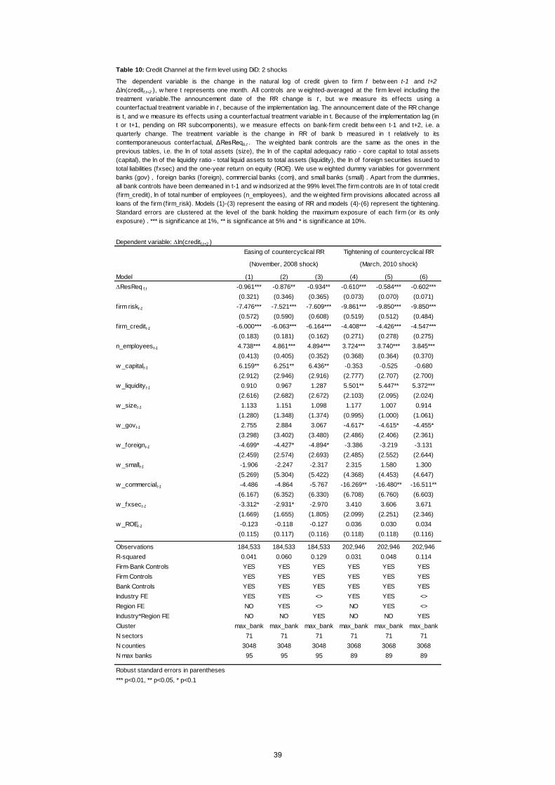
Dependent variable: Dln(creditf,t+2 )

Model (1) (2) (3) (4) (5) (6)

DResReq f,t -0.961*** -0.876** -0.934** -0.610*** -0.584*** -0.602***

(0.321) (0.346) (0.365) (0.073) (0.070) (0.071)

firm riskt-1 -7.476*** -7.521*** -7.609*** -9.861*** -9.850*** -9.850***

(0.572) (0.590) (0.608) (0.519) (0.512) (0.484)

firm_creditt-1 -6.000*** -6.063*** -6.164*** -4.408*** -4.426*** -4.547***

(0.183) (0.181) (0.162) (0.271) (0.278) (0.275)

n_employees t-1 4.738*** 4.861*** 4.894*** 3.724*** 3.740*** 3.845***

(0.413) (0.405) (0.352) (0.368) (0.364) (0.370)

w _capitalt-1 6.159** 6.251** 6.436** -0.353 -0.525 -0.680

(2.912) (2.946) (2.916) (2.777) (2.707) (2.700)

w _liquidity t-1 0.910 0.967 1.287 5.501** 5.447** 5.372***

(2.616) (2.682) (2.672) (2.103) (2.095) (2.024)

w _sizet-1 1.133 1.151 1.098 1.177 1.007 0.914

(1.280) (1.348) (1.374) (0.995) (1.000) (1.061)

w _govt-1 2.755 2.884 3.067 -4.617* -4.615* -4.455*

(3.298) (3.402) (3.480) (2.486) (2.406) (2.361)

w _foreignt-1 -4.699* -4.427* -4.894* -3.386 -3.219 -3.131

(2.459) (2.574) (2.693) (2.485) (2.552) (2.644)

w _smallt-1 -1.906 -2.247 -2.317 2.315 1.580 1.300

(5.269) (5.304) (5.422) (4.368) (4.453) (4.647)

w _commercialt-1 -4.486 -4.864 -5.767 -16.269** -16.480** -16.511**

(6.167) (6.352) (6.330) (6.708) (6.760) (6.603)

w _fxsec t-1 -3.312* -2.931* -2.970 3.410 3.606 3.671

(1.669) (1.655) (1.805) (2.099) (2.251) (2.346)

w _ROEt-1 -0.123 -0.118 -0.127 0.036 0.030 0.034

(0.115) (0.117) (0.116) (0.118) (0.118) (0.116)

Observations 184,533 184,533 184,533 202,946 202,946 202,946

R-squared 0.041 0.060 0.129 0.031 0.048 0.114

Firm-Bank Controls YES YES YES YES YES YES

Firm Controls YES YES YES YES YES YES

Bank Controls YES YES YES YES YES YES

Industry FE YES YES <> YES YES <>

Region FE NO YES <> NO YES <>

Industry*Region FE NO NO YES NO NO YES

Cluster max_bank max_bank max_bank max_bank max_bank max_bank

N sectors 71 71 71 71 71 71

N counties 3048 3048 3048 3068 3068 3068

N max banks 95 95 95 89 89 89


*** p<0.01, ** p<0.05, * p<0.1


(November, 2008 shock)


(March, 2010 shock)

The dependent variable is the change in the natural log of credit given to firm f betw een t-1 and t+2 ,

Δln(creditf,t+2 ), w here t represents one month. All controls are w eighted-averaged at the firm level including the

treatment variable.The announcement date of the RR change is t , but w e measure its effects using a

counterfactual treatment variable in t , because of the implementation lag. The announcement date of the RR change

is t, and w e measure its effects using a counterfactual treatment variable in t. Because of the implementation lag (in

t or t+1, pending on RR subcomponents), w e measure effects on bank-firm credit betw een t-1 and t+2, i.e. a

quarterly change. The treatment variable is the change in RR of bank b measured in t relatively to its

comtemporaneuous conterfactual, ΔResReqb,t . The w eighted bank controls are the same as the ones in the

previous tables, i.e. the ln of total assets (size), the ln of the capital adequacy ratio - core capital to total assets


total liabilities (fxsec) and the one-year return on equity (ROE). We use w eighted dummy variables for government

banks (gov) , foreign banks (foreign), commercial banks (com), and small banks (small) . Apart from the dummies,

all bank controls have been demeaned in t-1 and w indsorized at the 99% level.The f irm controls are ln of total credit

(f irm_credit), ln of total number of employees (n_employees), and the w eighted firm provisions allocated across all

loans of the firm (firm_risk). Models (1)-(3) represent the easing of RR and models (4)-(6) represent the tightening.

Standard errors are clustered at the level of the bank holding the maximum exposure of each firm (or its only

exposure) . *** is signif icance at 1%, ** is signif icance at 5% and * is signif icance at 10%.

Table 10: Credit Channel at the f irm level using DiD: 2 shocks

39


Model (1) (2) (3) (4) (5) (6) (7) (8) (9) (10)

DResReq b,t 0.306 0.281 0.217 0.003 0.022 0.391 0.374 0.407 0.672 0.666

(0.220) (0.210) (0.184) (0.419) (0.362) (0.344) (0.347) (0.282) (0.550) (0.456)

Observations 706,620 706,620 706,620 706,620 706,620 669,807 669,807 669,807 669,807 669,807

R-squared 0.000 0.009 0.328 0.013 0.331 0.001 0.010 0.324 0.016 0.328

Firm-Bank Controls NO YES YES YES YES NO YES YES YES YES

Firm Controls NO YES <> YES <> NO YES <> YES <>

Bank Controls NO NO NO YES YES NO NO NO YES YES

Firm FE NO NO YES NO YES NO NO YES NO YES

Cluster bank_id bank_id bank_id bank_id bank_id bank_id bank_id bank_id bank_id bank_id

DResReq Count. 08 Count. 08 Count. 08 Count. 08 Count. 08 Count. 10 Count. 10 Count. 10 Count. 10 Count. 10


*** p<0.01, ** p<0.05, * p<0.1

Table 11: Placebo Credit Channel using DiD: 2 shocks

In this table, w e reproduce Table 4 in one stable placebo period exactly one year after the second shock. Placebos are estimated

independently using the easing and tightening counterfactuals. The dependent variable is the change in the natural log of credit given by bank

b to firm f (intensive margin) betw een t+2 and t-1, Δln(creditb,f,t+2 ), w here t represents one month. The announcement date of the RR change is

t, and w e measure its effects using a counterfactual treatment variable in t. Because of the implementation lag (in t or t+1, pending on RR

subcomponents), w e measure effects on bank-firm credit betw een t-1 and t+2, i.e. a quarterly change. The treatment variable is the change in

RR of bank b measured in t relatively to its comtemporaneuous conterfactual, DResReq b,t. The bank controls are the ln of total assets (size),

the ln of the capital adequacy ratio or core capital to total assets (capital), the ln of the liquidity ratio - total liquid assets to total assets (liquidity),

the ln of foreign securities issued to total liabilities (fxsec) and the one-year return on equity (ROE). We use a dummy variable for government

banks (gov) , foreign banks (foreign), commercial banks (commercial) and small banks (small). Apart from the dummies, all bank controls have

been demeaned in t-1 and w indsorized at the 99% level.The firm controls are ln of total credit (f irm_credit), and the ln of the firms´ number of

employees (n_employees) , f irm sector (sector) and county level dummies (municipality). The firm-bank control is the w eighted firm-bank

provisions allocated across all loans of these firm-bank relationship (risk). Models (1)-(5) represent the loosening of RR and models (6)-(10)

represent the tightening. Models (1) and (6) represent our are least saturated regression using only ΔResReqb,t as an explanatory variable.

Models (2) and (7) introduce firm and firm-bank controls. Models (3) and (8) introduce firm FE. Models (4) and (9) introduce bank controls

(w ithout firm FE); and, models (5) and (10) represent our most saturated regressions w ith FE and bank controls. Standard errors are clustered

at the bank level. *** is signif icance at 1%, ** is signif icance at 5% and * is signif icance at 10%.

Easing of countercyclical RR Tightening of countercyclical RR

(March, 2011 placebo shock) (March, 2011 placebo shock)

40


Model (1) (2) (3) (4) (5) (6) (7) (8) (9) (10) (11)

DResReq t -0.186 -0.183 -0.233 -0.190 -0.178 -0.137 -0.185 -0.131 -0.207* -0.194 -0.141

(0.156) (0.160) (0.140) (0.156) (0.147) (0.163) (0.173) (0.156) (0.120) (0.150) (0.251)

DResReq t

* CAR t-1 -0.557 -1.568

(0.636) (1.482)

* liquidity t-1 2.585** 2.539*

(0.950) (1.307)

* non-core t-1 -1.307 0.192

(1.163) (1.930)

* fxsec t-1 8.338*** 7.398

(2.312) (4.541)

*size t-1 -0.107* -0.091

(0.058) (0.107)

* importance t-1 -0.383 -0.521

(0.251) (0.370)

* GDPt-1 -15.642 -16.751*

(9.522) (9.141)

* Selict-1 -1.325*** -1.227**

(0.407) (0.514)

* firm risk t-1 -0.259 -0.271

(0.897) (0.834)

Observations 14,504,485 14,504,485 14,504,485 14,504,485 14,504,485 14,504,485 14,504,485 14,504,485 14,504,485 14,504,485 14,504,485

R-squared 0.150 0.150 0.150 0.150 0.150 0.150 0.150 0.151 0.151 0.151 0.151

Firm-Bank Controls YES YES YES YES YES YES YES YES YES YES YES

Firm Controls <> <> <> <> <> <> <> <> <> <> <>

Bank Controls YES YES YES YES YES YES YES YES YES YES YES

Bank-Firm FE YES YES YES YES YES YES YES YES YES YES YES


*** p<0.01, ** p<0.05, * p<0.1

Appendix 1. Credit Channel using Long Panel: bank and firm heterogeneity

The dependent variable is the change in the natural log of credit given by bank b to firm f (intensive margin) between t+1 and t , Dln(credit b,f,t+1), where t is in

quarters. The announcement and the change in RR are observed during quarter t and we measure its effects on the following quarter using an index. For instance,

one tightening is identified as a +1 change in the index, and a loosening as a -1. We present the main results for the treatment group, i.e. dummy variable for the

banks belonging to conglomerates that are affected by the policies (treat). The control group, i.e. small independent banks represnt the unaffected bank

institutions. The bank controls are the natural log (ln) of bank assets (size), the ln of the capital adequacy ratio - core capital to total assets (CAR), the ln of the

liquidity ratio - total liquid assets to total assets (liquidity), the ln of non-performing loans to total credit (NPL), the ln of non-core liabilities to total liabilties (non-

core), the ln of foreign securities issued to total liabilities (fxsec), a dummy variable for commercial banks, a dummy variable for banks that belong to a bank

conglomerate, and a dummy variable for small bank institutions. The firm-bank controls are the share of firm-bank credit to bank capital (importance), the share of

firm-bank credit to total firm credit (market_share), the weighted firm-bank provisions allocated across all loans of these firm-bank relationship (risk), the share of

credit lines to total exposure (scline), a dummy variable for firm-bank relationships with loans indexed in foreign currency (foreign_currency) and a dummy variable

for loans in default. All bank and firm-bank controls are measured in the previous quarter, t-1. Apart from the dummies, all bank controls have been demeaned in t-

1 and windsorized at the 98% level.All models have Firm and Time FE. Standard errors are clustered at the bank level. *** is significance at 1%, ** is significance

at 5% and * is significance at 10%.

41


Model (1) (2) (3) (4) (5) (6) (7) (8) (9) (10) (11)

SDResReq t -2.089*** -2.237*** -2.250** -2.219*** -2.026** -2.095*** -2.086*** -2.243 -0.588 -2.026*** -2.528***

(0.645) (0.706) (0.886) (0.663) (0.799) (0.678) (0.646) (1.392) (0.982) (0.654) (0.937)

SDResReq t

* CAR t-1 -1.841 -1.986

(1.670) (3.997)

* liquidity t-1 6.002*** 7.534**

(2.240) (3.092)

* non-core t-1 -2.605 0.00979

(1.954) (3.994)

* fxsec t-1 4.987 9.499

(11.23) (13.33)

*size t-1 -0.0810 -0.0401

(0.117) (0.195)

* importance t-1 -0.409 -0.440

(0.391) (0.558)

* GDPt-1 9.507

(21.34)

* Selict-1 -6.961***

(2.297)

* firm risk t-1 -0.0569 1.274

(1.870) (2.585)

Observations 14,504,485 14,504,485 14,504,485 14,504,485 14,504,485 14,504,485 14,504,485 14,504,485 14,504,485 14,504,485 14,504,485

R-squared 0.151 0.151 0.151 0.151 0.151 0.151 0.151 0.151 0.152 0.152 0.152

Firm-Bank Controls YES YES YES YES YES YES YES YES YES YES YES

Firm Controls <> <> <> <> <> <> <> <> <> <> <>

Bank Controls YES YES YES YES YES YES YES YES YES YES YES

Bank-Firm FE YES YES YES YES YES YES YES YES YES YES YES

The dependent variable is the change in the natural log of credit given by bank b to firm f (intensive margin) between t+1 and t , Dln(credit b,f,t+1), where t is in

quarters. The announcement and the change in RR are observed during quarter t and we measure its effects on the following quarter using an index. For instance,

one tightening is identified as a +1 change in the index, and a loosening as a -1. This is the distributed lags model and the coefficients represent the one-year

accumulated average effect (across all shocks), i.e. treatment group dummy variable (treat) is interacted with Dln(credit b,f,t+1) and all controls in four lags

independently. Coefficients and standard erros are calculated after that to reflect the accumulated results of these four lags' interactions. The bank controls are

the natural log (ln) of bank assets (size), the ln of the capital adequacy ratio - core capital to total assets (CAR), the ln of the liquidity ratio - total liquid assets to

total assets (liquidity), the ln of non-performing loans to total credit (NPL), the ln of non-core liabilities to total liabilties (nocore), the ln of foreign securities issued

to total liabilities (fxsec), a dummy variable for commercial banks, a dummy variable for banks that belong to a bank conglomerate, and a dummy variable for

small independent bank institutions (mostly unaffected by RR changes). The firm-bank controls are the share of firm-bank credit to bank capital (importance), the

share of firm-bank credit to total firm credit (market_share), the weighted firm-bank provisions allocated across all loans of these firm-bank relationship (risk), and

a dummy variable for firm-bank relationships with loans indexed in foreign currency (foreign_currency). All bank and firm-bank controls are measured in the

previous quarter, t-1.We introduce four lags of controls accordingly. Apart from the dummies, all bank controls have been demeaned in t-1 and windsorized at the

98% level.All models have firm and Time FE. Standard errors are clustered at the bank level. *** is significance at 1%, ** is significance at 5% and * is

significance at 10%.

Appendix 2. Credit Channel using Long Panel: bank and firm heterogeneity (distributed lags)

42

Documents

Credit Supply Responses to Reserve Requirement: loan … · Credit Supply Responses to Reserve Requirement: loan-level evidence from macroprudential policye Requirement: loan-level