Embed Size (px)
Citation preview

Credit Risk and Nonlinear Filtering: Computational Aspects andEmpirical Evidence
Thesis by
Agostino Capponi
In Partial Fulfillment of the Requirements
for the Degree of
Doctor of Philosophy
California Institute of Technology
Pasadena, California
2009
(Defended May 27, 2009)

ii
c© 2009
Agostino Capponi
All Rights Reserved

iii
To my family.

iv
Acknowledgements
I would like to express my gratitude to the outstanding Caltech environment which allowed me to conduct
my research in a stimulating and very constructive way. I consider myself very fortunate for having the
opportunity to work in this highly stimulating intellectual atmosphere. I would like to express my gratitude
to my advisor, Prof. Jaksa Cvitanic, for providing guidance and assistance throughout the period of my
PhD research. He has always been available and supportive and helped me to become familiar with the field
of credit risk. I would also like to thank Prof. K. Mani Chandy for his great participation in my research
work during all my stay at Caltech and for serving on my committee. I would like to thank Prof. John O.
Ledyard for serving on my committee and giving me the possibility to present the results of my research work
at SISL seminars on a regular basis. Those seminars have been sources of ideas and constructive criticism.
They had a significant impact on my PhD work and improved substantially my presentation skills. I would
also like to thank the other member of my committee, Prof. Yaser Abu-Mostafa for reading my work. I
would like to thank the SISL grants that supported my PhD research during all these years at Caltech. I
would also like to thank those people who made life at Caltech more enjoyable; thanks to all colleagues and
friends for their company and for sharing with me some of the best moments in my life. Finally but most
importantly, I would like to express my deepest gratitude to my parents and Concetta for their endless love
and unconditional support; without their sacrifices, it would have been impossible for me to reach this point
of my life.

v
Abstract
This thesis proposes a novel credit risk model which deals with incomplete information on the firm’s as-
set value. Such incompleteness is due to reporting bias deliberately introduced by insider managers and
executives of the firm and unobserved by outsiders.
The pricing of corporate securities and the evaluation of default measures in our credit risk framework
requires the solution of a computationally unfeasible nonlinear filtering problem. We propose a polynomial
time-sequential Bayesian approximation scheme which employs convex optimization methods to iteratively
approximate the optimal conditional density of the state on the basis of received market observations.
We also provide an upper bound on the total variation distance between the actual filter density and our
approximate estimator. We use the filter estimator to derive analytical expressions for the price of corporate
securities (bond and equity) as well as for default measures (default probabilities, recovery rates, and credit
spreads) under our credit risk framework. We propose a novel statistical calibration method to recover the
parameters of our credit risk model from market price of equity and balance sheet indicators. We apply the
method to the Parmalat case, a real case of misreporting and show that the model is able to successfully
isolate the misreporting component. We also provide empirical evidence that the term structure of credit
default swaps quotes exhibits special patterns in cases of misreporting by using three well known cases of
accounting irregularities in US history: Tyco, Enron, and WorldCom.
We conclude the thesis with a study of bilateral credit risk, which accommodates the case in which both
parties of the financial contract may default on their payments. We introduce the general arbitrage-free
valuation framework for counterparty risk adjustments in presence of bilateral default risk. We illustrate
the symmetry in the valuation and show that the adjustment involves a long position in a put option plus a
short position in a call option, both with zero strike and written on the residual net value of the contract at
the relevant default times. We allow for correlation between the default times of each party of the contract
and the underlying portfolio risk factors. We introduce stochastic intensity models and a trivariate copula
function on the default times exponential variables to model default dependence. We provide evidence
that both default correlation and credit spread volatilities have a relevant and structured impact on the
adjustment. We also study a case involving British Airways, Lehman Brothers, and Royal Dutch Shell,
illustrating the bilateral adjustments in concrete crisis situations.

vi
Contents
Acknowledgements iv
Abstract v
1 Introduction 1
1.1 Background . . . . . . . . . . . . . . . . . . . . . . . . . . . . . . . . . . . . . . . . . . . . . . 1
1.2 Summary of Contributions and Overview of the Thesis . . . . . . . . . . . . . . . . . . . . . . 3
2 Preliminaries and Definitions 5
2.1 Notation and Terminology . . . . . . . . . . . . . . . . . . . . . . . . . . . . . . . . . . . . . . 5
2.2 Structural Models . . . . . . . . . . . . . . . . . . . . . . . . . . . . . . . . . . . . . . . . . . 6
2.2.1 The Merton Model . . . . . . . . . . . . . . . . . . . . . . . . . . . . . . . . . . . . . . 7
2.3 Actual versus Risk-Neutral Default Probabilities . . . . . . . . . . . . . . . . . . . . . . . . . 10
2.4 Reduced Form Models . . . . . . . . . . . . . . . . . . . . . . . . . . . . . . . . . . . . . . . . 11
2.5 Incomplete Information Models . . . . . . . . . . . . . . . . . . . . . . . . . . . . . . . . . . . 12
3 Credit Risk Modeling With Misreporting 15
3.1 Introduction . . . . . . . . . . . . . . . . . . . . . . . . . . . . . . . . . . . . . . . . . . . . . . 15
3.2 Estimating Risk of Misreporting . . . . . . . . . . . . . . . . . . . . . . . . . . . . . . . . . . 16
3.3 Model Definition . . . . . . . . . . . . . . . . . . . . . . . . . . . . . . . . . . . . . . . . . . . 18
3.4 Structural Model with Misreporting . . . . . . . . . . . . . . . . . . . . . . . . . . . . . . . . 19
3.4.1 The Pricing Framework . . . . . . . . . . . . . . . . . . . . . . . . . . . . . . . . . . . 19
3.4.2 Exact Filtering . . . . . . . . . . . . . . . . . . . . . . . . . . . . . . . . . . . . . . . . 21
3.4.3 Equity and Bond Prices . . . . . . . . . . . . . . . . . . . . . . . . . . . . . . . . . . . 21
3.5 Bond and Equity Price Computation . . . . . . . . . . . . . . . . . . . . . . . . . . . . . . . . 22
3.5.1 Approximate Bond and Equity Prices . . . . . . . . . . . . . . . . . . . . . . . . . . . 23
3.6 Computation of Default Measures . . . . . . . . . . . . . . . . . . . . . . . . . . . . . . . . . . 24
3.6.1 Default Probability . . . . . . . . . . . . . . . . . . . . . . . . . . . . . . . . . . . . . . 24
3.6.2 Expected Recovery Rate . . . . . . . . . . . . . . . . . . . . . . . . . . . . . . . . . . . 25
3.6.3 The Term Structure of Credit Spreads . . . . . . . . . . . . . . . . . . . . . . . . . . . 26

vii
4 Empirical Analysis of misreporting: Model Calibration and Statistical Analysis 29
4.1 Introduction . . . . . . . . . . . . . . . . . . . . . . . . . . . . . . . . . . . . . . . . . . . . . . 29
4.2 Statistical Calibration . . . . . . . . . . . . . . . . . . . . . . . . . . . . . . . . . . . . . . . . 29
4.2.1 Estimation Procedure for Merton Model . . . . . . . . . . . . . . . . . . . . . . . . . . 29
4.2.2 Estimation Procedure for the Proposed Model . . . . . . . . . . . . . . . . . . . . . . 30
4.2.3 Application to the Parmalat Case . . . . . . . . . . . . . . . . . . . . . . . . . . . . . 32
4.3 Empirical Analysis of Misreporting . . . . . . . . . . . . . . . . . . . . . . . . . . . . . . . . . 34
4.3.1 CDS Contracts . . . . . . . . . . . . . . . . . . . . . . . . . . . . . . . . . . . . . . . . 34
4.3.2 CDS-Implied Default Probabilities . . . . . . . . . . . . . . . . . . . . . . . . . . . . . 35
4.3.3 Signals of Misreporting Inferred from CDS . . . . . . . . . . . . . . . . . . . . . . . . 36
5 Stochastic Filtering For Jump Systems 42
5.1 Setup and Problem Formulation . . . . . . . . . . . . . . . . . . . . . . . . . . . . . . . . . . 43
5.2 Exact Filter Derivation . . . . . . . . . . . . . . . . . . . . . . . . . . . . . . . . . . . . . . . 44
5.3 The Filter Approximation Scheme . . . . . . . . . . . . . . . . . . . . . . . . . . . . . . . . . 45
5.3.1 The Approximation Method . . . . . . . . . . . . . . . . . . . . . . . . . . . . . . . . . 45
5.3.2 Sparsity of the approximation . . . . . . . . . . . . . . . . . . . . . . . . . . . . . . . . 47
5.3.3 The Filter Approximation . . . . . . . . . . . . . . . . . . . . . . . . . . . . . . . . . . 48
5.3.4 Distance between Approximate and Optimal Filter . . . . . . . . . . . . . . . . . . . . 50
5.3.5 Computational Requirements . . . . . . . . . . . . . . . . . . . . . . . . . . . . . . . . 52
5.3.6 Quantitative Evaluation of the TVD . . . . . . . . . . . . . . . . . . . . . . . . . . . . 53
5.4 A Target Tracking Example . . . . . . . . . . . . . . . . . . . . . . . . . . . . . . . . . . . . . 55
6 Bilateral Counterparty Risk Valuation 59
6.1 Introduction . . . . . . . . . . . . . . . . . . . . . . . . . . . . . . . . . . . . . . . . . . . . . . 59
6.2 Arbitrage-Free Valuation of Bilateral Counterparty Risk . . . . . . . . . . . . . . . . . . . . . 61
6.3 Application to Credit Default Swaps . . . . . . . . . . . . . . . . . . . . . . . . . . . . . . . . 64
6.3.1 CDS Payoff . . . . . . . . . . . . . . . . . . . . . . . . . . . . . . . . . . . . . . . . . . 64
6.3.2 Default Correlation . . . . . . . . . . . . . . . . . . . . . . . . . . . . . . . . . . . . . . 65
6.3.3 CIR Stochastic Intensity Model . . . . . . . . . . . . . . . . . . . . . . . . . . . . . . . 66
6.3.4 Bilateral Risk Credit Valuation Adjustment for Receiver CDS . . . . . . . . . . . . . . 67
6.4 Monte-Carlo Evaluation of the BR-CVA Adjustment . . . . . . . . . . . . . . . . . . . . . . . 68
6.4.1 Simulation of CIR Process . . . . . . . . . . . . . . . . . . . . . . . . . . . . . . . . . . 68
6.4.2 Calculation of Survival Probability . . . . . . . . . . . . . . . . . . . . . . . . . . . . . 68
6.4.3 The Numerical BR-CVA Adjustment Algorithm . . . . . . . . . . . . . . . . . . . . . 69
6.5 Numerical Results . . . . . . . . . . . . . . . . . . . . . . . . . . . . . . . . . . . . . . . . . . 69
6.6 Application to a Market Scenario . . . . . . . . . . . . . . . . . . . . . . . . . . . . . . . . . . 76
6.7 Conclusions . . . . . . . . . . . . . . . . . . . . . . . . . . . . . . . . . . . . . . . . . . . . . . 80

viii
7 Conclusions 81
7.1 Concluding Remarks . . . . . . . . . . . . . . . . . . . . . . . . . . . . . . . . . . . . . . . . . 81
7.2 Future Work . . . . . . . . . . . . . . . . . . . . . . . . . . . . . . . . . . . . . . . . . . . . . 82
A Chapter 3: Bond and Equity Prices 88
B Chapter 3: Approximate Bond and Equity Prices 90
C Chapter 3: Bivariate Integrals 92
D Chapter 3: Probability of Default 93
E Chapter 3: Recovery Rate 95
F Chapter 5: Facts about Lipschitz Functions 97
G Chapter 5: Total Variation distance at initial time 98
H Chapter 5: Total Variation Distance at Time k 101
I Chapter 6: Brief Overview of Copula Functions 104
J Chapter 6: Proof of the General Counterparty Risk Pricing Formula 105
K Chapter 6: Proof of the Survival Probability Formula 108

ix
List of Figures
1.1 Schematic diagram of a bond’s cash flow . . . . . . . . . . . . . . . . . . . . . . . . . . . . . . . 2
1.2 Credit risk decomposition . . . . . . . . . . . . . . . . . . . . . . . . . . . . . . . . . . . . . . . 3
1.3 Defaulted bonds as a percentage of face value outstanding . . . . . . . . . . . . . . . . . . . . . 4
2.1 Schematic diagram of the Merton model . . . . . . . . . . . . . . . . . . . . . . . . . . . . . . . 8
3.1 Probability of fraud estimated by the model . . . . . . . . . . . . . . . . . . . . . . . . . . . . . 18
4.1 Parmalat crisis . . . . . . . . . . . . . . . . . . . . . . . . . . . . . . . . . . . . . . . . . . . . . 33
4.2 Schematic illustration of a CDS contract . . . . . . . . . . . . . . . . . . . . . . . . . . . . . . 34
4.3 1 year, 3 year, and 5 year CDS of Tyco . . . . . . . . . . . . . . . . . . . . . . . . . . . . . . . 37
4.4 1 year, 3 year, and 5 year CDS implied default probability of Tyco . . . . . . . . . . . . . . . . 37
4.5 1 year, 3 year, and 5 year CDS of WorldCom . . . . . . . . . . . . . . . . . . . . . . . . . . . . 38
4.6 1 year, 3 year, and 5 year CDS implied default probability of WorldCom . . . . . . . . . . . . . 39
4.7 1 year, 3 year, and 5 year CDS of Enron . . . . . . . . . . . . . . . . . . . . . . . . . . . . . . . 40
4.8 1 year, 3 year, and 5 year CDS implied default probability of Enron . . . . . . . . . . . . . . . 40
5.1 One cycle of the estimator . . . . . . . . . . . . . . . . . . . . . . . . . . . . . . . . . . . . . . . 50
5.2 Upper bound on the total variation distance for p1k,k(x) . . . . . . . . . . . . . . . . . . . . . . 54
5.3 Upper bound on the total variation distance for p2k,k(x) . . . . . . . . . . . . . . . . . . . . . . 55
5.4 Actual versus expected trajectory of the aircraft . . . . . . . . . . . . . . . . . . . . . . . . . . 55
5.5 Coordinate-combined position estimation error . . . . . . . . . . . . . . . . . . . . . . . . . . . 57
5.6 Coordinate-combined velocity estimation error . . . . . . . . . . . . . . . . . . . . . . . . . . . 57
5.7 The number of nonzero Gaussian components used in the density approximations p1k,k(x) and
p2k,k(x) . . . . . . . . . . . . . . . . . . . . . . . . . . . . . . . . . . . . . . . . . . . . . . . . . 58

x
List of Tables
2.1 Payoffs at maturity in Merton model . . . . . . . . . . . . . . . . . . . . . . . . . . . . . . . . . 7
3.1 Model predictors . . . . . . . . . . . . . . . . . . . . . . . . . . . . . . . . . . . . . . . . . . . . 17
3.2 Values of predictors . . . . . . . . . . . . . . . . . . . . . . . . . . . . . . . . . . . . . . . . . . 18
4.1 Parameter estimates . . . . . . . . . . . . . . . . . . . . . . . . . . . . . . . . . . . . . . . . . . 33
6.1 The credit risk levels and credit risk volatilities parameterizing the CIR processes . . . . . . . 70
6.2 Break-even spreads in basis points generated using the parameters of the CIR processes in
Table 6.1. The first column is generated using low credit risk and credit risk volatility. The
second column is generated using middle credit risk and credit risk volatility. The third column
is generated using high credit risk and credit risk volatility. . . . . . . . . . . . . . . . . . . . . 71
6.3 BR-CVA in basis points for the case when ν2 = 0.01 and ν0 = 0.01; numbers within round
brackets represent the Monte-Carlo standard error. The CDS contract on the reference credit
has a five-years maturity. . . . . . . . . . . . . . . . . . . . . . . . . . . . . . . . . . . . . . . . 73
6.4 BR-CVA in basis points for the case when ν2 = 0.2 and ν0 = 0.01; numbers within round
brackets represent the Monte-Carlo standard error. The CDS contract on the reference credit
has a five-years maturity. . . . . . . . . . . . . . . . . . . . . . . . . . . . . . . . . . . . . . . . 73
6.5 BR-CVA under five different riskiness scenarios. The CIR volatilities are set to ν0 = ν1 = ν2 =
0.1. The correlation triple has only one nonzero entry . . . . . . . . . . . . . . . . . . . . . . . 74
6.6 BR-CVA under five different riskiness scenarios. The CIR volatilities are set to ν0 = ν1 = ν2 =
0.1. The correlation triple has two nonzero entries . . . . . . . . . . . . . . . . . . . . . . . . . 75
6.7 BR-CVA under five different riskiness scenarios. The CIR volatilities are set to ν0 = ν1 = ν2 =
0.1. The correlation triple has all nonzero entries . . . . . . . . . . . . . . . . . . . . . . . . . . 75
6.8 Market spread quotes in basis points for Royal Dutch Shell, Lehman Brothers, and British
Airways on January 5, 2006 . . . . . . . . . . . . . . . . . . . . . . . . . . . . . . . . . . . . . . 76
6.9 Market spread quotes in basis points for Royal Dutch Shell, Lehman Brothers and British
Airways on May 1, 2008 . . . . . . . . . . . . . . . . . . . . . . . . . . . . . . . . . . . . . . . . 76
6.10 The CIR parameters of Lehman Brothers, Royal Dutch Shell, and British Airways calibrated
to the market quotes of CDS on January 5, 2006 . . . . . . . . . . . . . . . . . . . . . . . . . . 77
xi
6.11 Value of the CDS contract between British Airways and Lehman Brothers on default of Royal
Dutch Shell agreed on January 5, 2006, and marked to market by British Airways on May 1,
2008. The pairs (LEH Pay, BAB Rec) and (BAB Pay, LEH Rec) denote respectively the mark-
to-market value when British Airways is the CDS receiver and CDS payer. The mark-to-market
value of the CDS contract without risk adjustment when British Airways is respectively payer
(receiver) is 84.2(-84.2) bps, due to the widening of the CDS spread curve of Royal Dutch Shell. 78
6.12 Value of the CDS contract between British Airways and Royal Dutch Shell on default of Lehman
Brothers agreed on January 5, 2006, and marked to market by British Airways on May 1, 2008.
The pairs (RDSPLC Pay, BAB Rec) and (BAB Pay, RDSPLC Rec) denote respectively the
mark-to-market value when British Airways is the CDS receiver and CDS payer. The mark-to-
market value of the CDS contract without risk adjustment when British Airways is respectively
payer (receiver) is 529(-529) bps, due to the widening of the CDS spread curve of Lehman
Brothers. . . . . . . . . . . . . . . . . . . . . . . . . . . . . . . . . . . . . . . . . . . . . . . . . 79

1
Chapter 1
Introduction
1.1 Background
Credit risk is the risk of default or of reductions in market value caused by changes in the credit quality of
issuer or counterparties. The distribution of credit losses is complex. At its center is the probability of default,
by which we mean any type of failure to honor a financial agreement. The estimation of the probability
of default requires specifying a model of investor uncertainty, a model of the available information and its
evolution over time, and a model for the default event. However, default probabilities alone would not be
sufficient to price credit-sensitive securities. We would need to know how much the marketplace charges for
holding risky assets, meaning assets subject to risk of default. This in turn requires the specification of a
model of recovery upon default, and most importantly a model of the premium that investors require as
compensation for bearing credit risk.
Although credit denotes the extension of access to any liquid assets today in return for a promise to pay
in the future, when we think of credit we typically think of the debt that one party owes to another and
this will also be the case for this thesis. In a debt transaction, there is usually a lender and a borrower. A
common form of credit is a bond, which is an interest-bearing certificate issued by a government or business
promising to pay the holder a specified sum on a specified date.
Bonds can be issued by the government, the so called Treasury bonds, or by corporations, thereby named
corporate bonds. Treasury bonds are typically assumed to be risk-free in countries with stable economies,
and this is supported by the fact that the government can always either raise taxes or print out more money
as a last resort to pay back debt. Under the simplest assumptions and using semi-annual compounding, the
price of a treasury coupon paying bond with face value 100 dollars would be given by
Btreas =2T∑n=1
c/2(1 + y
2 )n/2+
100(1 + y)T
(1.1.1)
where c is the paid coupon and y the treasury yield. Corporate bonds instead are exposed to a default risk
with magnitude depending on the financial health of the particular issuer and its ability to raise revenue.
Under the same scenario as above, the price of a corporate coupon paying bond is given by:

2
PV
C/2
0 Time (Years)Maturity
Coupons
Principal(from Borrower)
Principal(from Lender)
0.5 1 1.5 2 2.5 3 3.5 4
C/2 C/2 C/2 C/2 C/2 C/2
C/2
P
Coupon
Figure 1.1: Schematic diagram of a bond’s cash flow
Bcorp =2T∑n=1
c/2(1 + y+s
2 )n/2+
100(1 + y+s
2 )T(1.1.2)
It appears from Eq. (1.1.1) and Eq. (1.1.2) that the price difference between the two bonds depends on
the term s, which is called the credit spread. The larger the credit spread, the smaller the relative price of
corporate bond with respect to treasury bond. The credit spread is a key concept and denotes the additional
compensation that the holders of risky assets are demanding for bearing the default risk. If no additional
compensation is offered to holders of the corporate bonds, then they would be better off buying the treasury
bond.
Intuitively, we can decompose the yield spread into the three categories, see Figure 1.2. The default risk
is the risk due to the potential loss associated with a single default and depends on the amount recovered. If
the default time and recovery value were known, then it would be possible to diversify the risk and construct
a portfolio consisting of names having specified likelihood of losses which guarantees on average the risk-free
rate. In years when default did not occur, the bond would return a little more due to the expected loss
premium. However, in the event of default, it would return much less. Since an investor could obtain the
risk-free base rate not just “on average”, but all the time by buying the risk free bond, the risky bond must
provide additional compensatory return. This indicates that there is an amount of nondiversifiable credit
risk and that the market provides compensation for this unavoidable risk bearing. Such component is called
risk premium and includes uncertainty regarding default timing, recovery value, and accuracy of revealed
information for which investors ought to be compensated. The final source of risk is liquidity risk, and refers
to the chance that the company may have insufficient cash flow to meet its obligations due to the lack of
marketability of an investment that cannot be bought or sold quickly enough by the company to fulfill its
obligation.

3
Yield
Default Risk
Liquidity Risk
Risk Premium
Maturity
Figure 1.2: Credit risk decomposition
Much research is devoted to separate out the effects of all of these variables when computing the spread
of corporate bond yields to US Treasury. Default modeling is becoming a major problem nowadays due
to the credit crunch crisis which we are experiencing, and it is also an important tool which is daily used
for hedging credit exposures. This importance is confirmed by Figure 1.3 which shows the distribution of
defaulted debt as a percentage of the total amount of outstanding debt.
It is evident from Figure 1.3 that defaulted debt accounts for more than 5% of the total outstanding
debt, thus motivating the enormous amount of academic and industrial research devoted to this topic.
1.2 Summary of Contributions and Overview of the Thesis
The main contributions of this thesis are
• Development of a novel credit risk model. Such model accounts for the possibility that the firm is
misrepresenting its accounting data. This model adds to the branch of credit risk literature focusing
on the role of incomplete information on pricing. The level of incompleteness derives from the fact
that the true asset value observed by outsiders may be biased and thus needs to be filtered out from
market- available information. We provide analytical expressions for corporate security prices and
default measures under the proposed modeling framework. These results are presented in Chapter
3 and have been published in the finance journal International Journal of Theoretical and Applied
Finance (see Capponi and Cvitanic, 2009).
• Development of a stochastic Bayesian filtering algorithm for jump linear jump systems with state-
dependent transitions. The mathematical framework of our credit risk model turns out to be a Hidden
Markov model, and more specifically a Markovian jump linear system with state-dependent transitions.

4
0%
2%
4%
6%
8%
10%
12%
1983
1984
1985
1986
1987
1988
1989
1990
1991
1992
1993
1994
1995
1996
1997
1998
1999
2000
2001
2002
2003
2004
2005
Def
ault
Rat
e
20%
30%
40%
50%
60%
70%
Recovery V
alue
DefaultMean: 5.1%
StdDev: 2.7%
RecoveryMean: 41.9%
StdDev: 10.0%
Figure 1.3: Defaulted bonds as a percentage of face value outstanding. Source: E. Altman and S. Jha.Market Size and Investment Performance of Defaulted Bonds and Bank Loans: 1987-2006. NYU SalomonCenter Publication, 2006.
We show that the problem of evaluating the optimal filtering density is computationally intractable and
then propose a polynomial time approximation method with guaranteed error bound to compute the
density. These results are presented in Chapter 5 and have been published in the journal Automatica
(see Capponi, 2009a).
• Development of a novel calibration algorithm for structural models of credit risk with incomplete
information. The algorithm combines maximum likelihood estimation methods along with option
price inversion approaches to recover drift, volatility, accounting noise variance, and reporting bias.
These results are presented in Chapter 4 and have been published in the proceedings of the IEEE
Conference on Computational Intelligence for Financial Engineering, where they were granted with
the best student paper award (see Capponi, 2009b).
• Framework for bilateral counterparty risk valuation. We introduce the general arbitrage-free valuation
framework for counterparty risk adjustments in presence of bilateral default risk, including default of
both investor and her counterparty. We show that the adjustment involves a long position in a put
option plus a short position in a call option, both with zero strike and written on the residual net value
of the contract at the relevant default times. We then specialize our analysis to Credit Default Swaps
and show the impact of credit spread volatility and default correlation on the bilateral credit risk value
adjustment. These results are presented in Chapter 6. A subset of these results has been submitted
for peer review publication to Risk magazine (see Brigo and Capponi) and a more extended version of
the work is currently in preparation for Finance and Stochastics.
Chapter 7 draws conclusions and discusses future problems of interest. More results and technical proofs
are provided in the appendices.

5
Chapter 2
Preliminaries and Definitions
In this chapter we provide notation and terminology which will be heavily used in the remainder of this
thesis. We also briefly describe the general taxonomy of credit risk models which is needed to understand
the results of this thesis. Those include structural models which use option pricing theory to evaluate credit
risk, reduced-form models using term structure theory to explain credit spread behavior and models with
incomplete information which provide a trade-off between the two. This is not intended to be a complete
survey and the interested reader is referred to books on the topic (see Lando, 2004).
2.1 Notation and Terminology
This section presents the basic notation and terminology.
• n(x;µ, σ): Gaussian density with mean µ and standard deviation σ
• n(x;µ,Σ): multivariate Gaussian density with mean µ and covariance Σ
• D(t, T ): price of a risk-free zero coupon bond maturing at T , as seen at time t
• B(t, T ): price of a defaultable zero coupon bond maturing at T , as seen at time t
• τ := T − t: time to maturity
• y(t, T ): yield of a corporate zero coupon bond maturing at T , as seen at time t
• r: risk-free rate
• CS(t, T ) := y(t, T ) − r: credit spread at maturity T as seen at time t. It is defined as the difference
between the yield of a defaultable zero coupon bond and a corresponding risk-free zero coupon bond
• ς: the default time indicator
• PD(t, T ): probability of defaulting at T as seen at time t
• RR(t, T ): recovery rate at time T as seen at time t

6
• BScall(t,Xt,K, T, σ): time t price of a Black Scholes call option with strike price K, volatility σ,
maturity T , and initial asset vale Xt
• BSput(t,Xt,K, T, σ): time t price of a Black Scholes put option with strike price K, volatility σ,
maturity T , and initial asset vale Xt
• λi,j(y) = P (θk = j|θk−1 = i,xk = y): mode switching probabilities
• λj(y) = P (θ0 = j|x0 = y): prior mode probability
• p(x|y, l) = P (xk = x|θk−1 = l,xk−1 = y): mode dependent transition density
• p(x) = P (x0 = x) : the initial density on x0
• plk|k(x) := P (xk = x, θk−1 = l|F zk ): the joint state-mode posterior hybrid density
• plk,k(x) := P (xk = x, θk−1 = l,F zk ): the unnormalized posterior density
• pk|k(x) = P (xk = x|F zk ): the posterior density
• Llk|k(x) = p(zk|xk = x, θk−1 = l): the mode conditioned measurement likelihood
• Ef [g] =∫Rn f(w)g(w)dw: the expectation of g with respect to the density f , where f and g are
functions
• F xk = σ(x1, x2, . . . , xk): the filtration generated by the state process x up to time k
• F zk = σ(z1, z2, . . . , zk): the filtration generated by the observation process z up to time k
• xl|k := E[xl|F zk ]: the conditional expectation of x at time l given the observation filtration at time k
• σ2l|k := E[(xl − xl|k)2|F z
k ] l > k: the conditional variance of x at time l given the observation
filtration at time k
2.2 Structural Models
In structural models, corporate liabilities are evaluated by decomposing their pay-offs in linear and nonlinear
products, and using standard option pricing theory to price them. Those models make explicit assumptions
about the dynamics of a firm’s assets and its capital structure, which are then used to determine the
occurrence of default. The literature on structural models goes back to Merton (1974), where the firm
defaults if, at the time of servicing the debt, its assets are below its outstanding debt. A more general
approach was introduced by Black and Cox (1976) who relax the Merton’s assumption and model default as
the first passage time of the firm’s asset value below a certain threshold. Further generalizations treat coupon
bonds, the effect of bond indenture provisions (see Geske, 1977), stochastic interest rates (see Longstaff and
Schwartz, 1995, Collin-Dufresne et al., 2004), and endogenous default barriers optimally triggered by equity
owners when the asset fall to a sufficiently low level (see Leland and Toft, 1996). Since this thesis builds

7
Assets Bonds EquityNo default VT ≥ K K VT −K
Default VT < K VT 0
Table 2.1: Payoffs at maturity in Merton model
upon the Merton model, we present it in some detail in this section and refer the interested reader to the
above references for a complete overview of structural models.
2.2.1 The Merton Model
Merton assumes that the firm is financed by equity and a zero coupon bond with face value K and maturity
date T . The firm’s contractual obligation is to repay the amount K to the bond investors at time T . Debt
covenants grant bond investors absolute priority: if the firm cannot fulfill its payment obligation, then bond
holders will immediately take over the firm. The payoff to equity and bond holders are summarized in Table
2.1.
If the asset value VT exceeds or equals the face value K of the bond, the bond holders will receive their
promised payment K and the shareholders will get the remaining VT −K. However, if the value of assets
VT is less than K, the ownership of the firm will be transferred to the bondholders, who lose the amount
K − VT . Equity is worthless because of limited liability. The asset value of the firm is assumed to follow a
log-normal diffusion process
dVt = µVtdt+ σVtdWt (2.2.1)
where µ is a drift parameter, σ > 0 is a volatility parameter, and Wt is a standard Brownian motion. Setting
m = µ− 0.5σ2, Ito’s lemma implies that
Vt = V0emt+σWt (2.2.2)
Figure 2.1 depicts the situation graphically. The bond payoff in Table 2.1 can be rewritten as
B(T, T ) = K −max[K − VT , 0] (2.2.3)
thus implying that the value of the defaultable zero coupon bond at any time t is given by
B(t, T ) = Ke−r(T−t) −BSput(t, Vt,K, T, σ) (2.2.4)
where r denotes the risk-free discount factor. The BSput(.) is also referred in the literature as the default
put option, since it measures the default risk of the bond.
As for equity, it follows from Table 2.1 that the final payoff can be expressed as
E(T, T ) = max[VT −K, 0] (2.2.5)

8
D
TimeT=1Y
mT σ
mt
log V0
Log-Asset Value
T0
Expected Log-Asset Value
Asset Volatility
Default Probability
Distribution ofLog-Asset Valueat Maturity
Sample Paths ofLog-Asset Value
Figure 2.1: The asset paths in the figure represent the uncertain future states of the firm’s assets, with thedistribution shown at time T representing the density of final asset states at that time. The probability ofdefault, PD, is given as the density of the distribution below the level of the debt (i.e., the proportion ofstates in which the firm is insolvent at time T).

9
thus implying that the equity value at any time t is given by
E(t, T ) = BScall(t, Vt,K, T, σ) (2.2.6)
Since WT is normally distributed with mean zero and variance T , the probability PD(t, T ) of defaulting
at time T as seen at time t is given by
PD(t, T ) = P (VT < K)
= P (σ(WT −Wt) < L−mτ)
= N
(L−mτ
σ√τ
)(2.2.7)
where L = log(KVt), and τ = T − t denotes the time to maturity.
Structural models are particularly elegant and informative, mainly because they impose an arbitrage
relationship between equity and debt. From this point of view, they provide a natural guideline for relative
value trades between the stock market and the credit derivatives market which is of utmost practical interest.
Moreover, models are forward looking and allow incorporating investors expectations of a firm’s future
performance. Unfortunately, these models result in a generally poor fit to market data due to several
limitations, some of which are outlined next.
• Typically, reasonable values for leverage of the firm and volatility of assets produce lower credit spreads
than those observed on the market.
• Undervaluation is particularly relevant for short term maturities: a typical credit term structure in
structural models shows a hump and zero intercept.
• Undervaluation is particularly relevant for high credit standing obligors.
• Bond prices play no role in estimating the value of the firm.
The first two items above represent an important concern for all structural models and have motivated a
lot of research, including this thesis. Those concerns arise from the fact that all structural models are based
on the assumption that the firm’s dynamic is regulated by a diffusion process and that the value of the firm
can be observed directly. Since diffusion processes have continuous sample paths and default is the first
hitting time of a barrier, then default is a predictable stopping time, and this leads to an underestimation of
the short-term credit spread as outlined above. From a mathematical point of view, this can be explained
using a key result from diffusion theory (see Karatzas and Shreve, 1995), stating that for any diffusion
process Xt
limh→0
P (|Xt+h −Xt| ≥ ε)h
= 0 (2.2.8)

10
We next show why this fact implies zero spread in the short term. Let us consider a risky zero coupon bond
paying the fact value K at time T if the issuing firm does not default, and zero otherwise. Differently from
the bond in the Merton model, such bond does not pay anything in case of default, thus it must have a lower
price and consequently a higher yield than the corresponding bond in the Merton model. The price of such
bond is obtained as
B(t, T ) := e−r(T−t)E[K1VT>K ]
= Ke−r(T−t)P (VT > K) (2.2.9)
The yield at time t of a bond maturing at T with principal K is defined as
y(t, T ) =1
T − tlog(
K
B(t, T )
)(2.2.10)
and since r is the yield of a zero-coupon risk free bond, we obtain that the time t credit spread for a bond
maturing at t+ h is given by
CS(t, t+ h) = − 1h
logB(t, t+ h)
K− r (2.2.11)
If we start at time t from a non-default state (Vt > K), then we have that
limh→0
CS(t, t+ h) = − 1h
logP (Vt+h > K|Vt > K)
≈ − 1h
(P (Vt+h > K|Vt > K)− 1)
=1hP (Vt+h ≤ K|Vt > K) (2.2.12)
Using Eq. (2.2.8), we can conclude that
limh→0
CS(t, t+ h) = 0 (2.2.13)
2.3 Actual versus Risk-Neutral Default Probabilities
The default probability given in Eq. (2.2.7) has been derived under historical measure, but it can be combined
with an equilibrium model of underlying expected returns to produce estimates of expected returns. We
can express an interesting relationship between the physical and risk-neutral world via the the capital asset
pricing model (CAPM). The premium over the risk-free rate that an investor should require to invest in
a risky asset depends on its holding period, volatility, and the current market price of risk. The CAPM

11
framework states
µ− r = β(µM − r)
=cov(µ, µM )
σ2M
(µM − r)
=cov(µ, µM )
σMσ
µM − r
σMσ
(2.3.1)
where µM is the market return and β is the covariance of the asset’s return with the market return relative
to the variance of the market. If we denote by ρ the correlation between the return of the asset and the
market return and
λ =µM − r
σM(2.3.2)
we can express the excess market return as:
µ− r = λρσ (2.3.3)
The parameter λ is called the market price of risk. It measures the tradeoffs between risk and return that
are made for securities depending on the asset values Vt. For an intuitive understanding of Eq. (2.3.3) notice
that the variable σ can be interpreted as the quantity of risk present in the asset value. On the right-hand
side, we are therefore multiplying the quantity of risk with its price, weighted by the correlation between
asset return and market return (the larger such correlation, the larger the potential gain resulting from the
investment in the risky asset Vt). The left-hand side is the expected return in excess of the risk-free interest
rate that is required to compensate for this risk. In other words, the term λρσ measures the extent that
the excess return required by investors on the firm’s securities is affected by the dependence on the asset. If
λρσ > 0, investors require a higher expected return to compensate for this risk; if λρσ < 0, the dependence
of the security on the firm’s asset value causes investors to require a lower return; if λρσ = 0, then the
investor does not require any extra compensation, which would imply that he is not taking any risk, thus its
return should be the same as investing at the risk-free rate r. When this is the case (i.e., µ = r, then we say
that we are in a risk-neutral world, and this is the framework assumed by the modern asset pricing theory
to determine the price of securities.
2.4 Reduced Form Models
Reduced form models go back to Artzner and Delbaen (1995), Jarrow and Turnbull (1995), and Duffie and
Singleton (1999). Unlike structural models, they do not argue why a firm defaults, but model default as a
Poisson-type event which occurs completely unexpectedly. The default time is defined as
ς = inft :∫ t
0
λsds ≥ Exp(1)
(2.4.1)

12
where Exp(1) denotes an exponentially distributed random variable with parameter 1. The process λs is a
stochastic process called the intensity process. It is an ad-hoc combination of financial variables often fit to
market spreads and is exogenously related to the the firms dynamics.
Eq. (2.4.1) implies immediately that the probability of non defaulting up to time T is given by
P (ς > T ) = e−R T0 λsds (2.4.2)
which leads to the pricing formula for the bond
B(t, T ) := e−r(T−t)E[K1ς>T ]
= Ke−r(T−t)Pς > T
= Ke−r(T−t)e−R T
tλsds (2.4.3)
If λs becomes constant, then Eq. (2.4.3) simplifies to
B(t, T ) = e−(r+λ)(T−t) (2.4.4)
and thus the credit spread is given by the constant λ.
The nice feature of reduced form model is that as t → T , the credit spreads do not approach zero,
but stay positive; we have seen an example above for the case when the intensity is constant. Therefore,
they remove the disturbing feature of zero-credit spreads in the short term. However, as evident from Eq.
(2.4.1), there is no natural link of defaults to the underlying dynamics of the firm‘s cash flows and financial
statements, thus those models are often criticized because they lose the micro-economic interpretation of the
default time.
2.5 Incomplete Information Models
The incomplete information framework attempts to unify structural and reduced form models under a
common perspective by taking the advantages of both methods. Underlying all credit models is the default
process. In traditional structural models default can be anticipated, and as seen in Section 2.2, there is no
short-term credit risk that would require compensation. In reduced form models, it is assumed that default
cannot be anticipated, so there is short-term credit risk by assumption, see Section 2.4. The default process
is parameterized through an intensity λ and model default probabilities and security prices are immediately
implied by the exogenous intensity dynamics. Instead of focusing on the default intensity and making ad-
hoc assumptions about its dynamics, incomplete information models specify the trend based on a model
definition of default. There are mainly two approaches to introduce short-term uncertainties into structural
models. The first possibility is to include jumps in the firm value, see Zhou (2001). In this situation, there is
always a chance that the firm value jumps below the default barrier, and thus default cannot be anticipated.

13
However, there is also a chance that the firm diffuses to the barrier, as in traditional structural models, and
in this case default can be anticipated. Thus, depending on the state of the world, there may or may not
be short-term credit risk. There is another approach which guarantees that default cannot be anticipated
and thus produces short-term credit risk. This approach is obtained after reconsidering the informational
assumptions underlying the traditional structural credit risk models which assume that the information used
to calibrate and run the model is observed perfectly. Such information includes the firm value process along
with its parameters, and the default barrier. In the incomplete information framework, we assume that the
information about these quantities is imperfect; this means that we are not sure either of the true value of
the firm or of the condition of the firm that will trigger default and consequently default becomes a complete
surprise. Several models with incomplete information have been proposed in the literature, some of which
are discussed next. Cetin et al. (2004) and Guo et al. (2009) propose an approach in which the market
is assumed to only partially observe, and possibly with a lag, relevant information concerning the state of
the firm. Brody et al. (2007) and Brody et al. (2008) derive bond pricing formulas in an economic model
where information about the actual cash flows of the debt obligation are obscured to market participants
by a Gaussian noise process which vanishes when the time of each required cash flow is reached. Giesecke
and Goldberg (2004) add incompleteness to structural models by assuming that the default barrier is a
stochastic process, thus investors cannot deduce the distance to default from the firm’s fundamentals as
in Merton or Black-Cox models. Frey and Runggaldier (2007) consider a model in which the intensity is
driven by unobserved state processes, and the calculation of measures of risk such as default probability
leads to a nonlinear filtering problem. In all these cases, default becomes an inaccessible stopping time for
the market, thus yielding a reduced form credit risk model. Duffie and Lando (2001) propose a model with
endogenous default threshold, but in which the market only observes noisy or delayed accounting reports
from which investors have to draw inference of the true asset value of the firm. This model creates a nonzero
instantaneous hazard rate of default, thus implying a nonzero short- term credit spread. Even further, they
prove that structural models with incomplete information are fully consistent with intensity models in the
sense that the instantaneous hazard rate of default is the intensity of the default indicator process with
respect to the information set observed in the market (noisy accounting reports), and not by the firm (true
state). We next report a sketch of the main results obtained in Duffie and Lando (2001), being those highly
related to the ones presented in this thesis, and we will provide a more detailed comparison in Chapter 3.
Their assumption is that the firm’s value is observed up to additive noise, namely Yt = Vt + Ut where Ut is
a white noise sequence. Let
ς = inft : Vt ≤ K (2.5.1)
and denote by f(x) the density on the initial asset value of the firm. Then we have
limh→0
1h
∫ ∞
0
P (ς ≤ h|V0 = x)f(x)dx =12σ2f ′(K) (2.5.2)

14
as opposed to the case when the initial asset value of the firm is known with certainty, in which case, using
the result in Eq. (2.2.8), we would obtain that PD(0, h) = 0.

15
Chapter 3
Credit Risk Modeling WithMisreporting
3.1 Introduction
In a statement released in 2007, the US Treasury Secretary complained about the huge number of accounting
data revisions in the US market. He claimed that some 1500 firms revise their balance sheet figures every
year, and that means, he claimed, that there must be something wrong with the system. So, the debate
on accounting transparency that arose at the beginning of the century is still open. Recent literature has
focused on the impact of these events on the evaluation of corporate liabilities, namely equity and bonds. On
theoretical grounds, Duffie and Lando (2001) was the first attempt to model the impact of accounting noise
on the credit spread term structure. On empirical grounds, Yu (2005) proved that accounting noise is actually
priced in the market: a risk premium is charged to the credit spreads of firms that adopt less transparency.
Fraud events that took place both in the US (Worldcom, Tyco, Enron, etc.) and in Europe (Cirio, Marconi,
Parmalat, etc.) in the first years of the century raised the issue of distinguishing between unbiased noise
due to measurement errors and cases of deliberate fraud. Inspired by these cases Cherubini and Manera
(2006) model the effect of deliberate misreporting on accounting statements through the introduction of
a probability of fraud which the market updates whenever new information about balance sheet is issued.
Brigo and Morini (2006) consider the effect of accounting reliability by modeling the ratio between the
level of default barrier and the value of company assets as a random variable, where pessimistic scenarios,
possibly corresponding to fraud in accounting, are associated with larger values of this ratio. None of the
above studies models explicitly the dynamics of misreporting.
We introduce a credit risk framework which incorporates the misreporting event as an intrinsic feature,
and is estimable using market and accounting data. We explicitly model the misreporting dynamics and
also calibrate a simple version of our model to the data for the Parmalat company around its bankruptcy.
The results indicate that the amount of misreporting was not negligible, and that by ignoring it, the model
would have resulted in a large overestimation of the firm’s volatility.
Misreporting may only arise if the market has incomplete knowledge of the manager’s objective function,
since then he may be better off with the option to misreport, see Fisher and Verrecchia (2000). If instead the
16
market is assumed to have rational expectations and perfect knowledge of manager’s objective, then it can
back out perfectly misreporting in equilibrium. We work under the incomplete knowledge assumption since
the exact nature of the manager’s compensation, his time horizon, and his litigation risk and reputation
costs associated with biased reporting are often unavailable to the market.
Although it is not easy to estimate the managerial risk of misreporting, recent studies have started
addressing this issue. For example, Wang (2007) proposes a bivariate probit model to recover the probability
of committing fraud from the probability of detected fraud. The rest of the chapter is organized as follows.
Section 3.2 describes and applies the Wang model to Tyco, a major case of misreporting. Section 3.3 describes
the components of the proposed model which deals with misreporting. Section 3.4 gives explicit formulas
for bond and equity prices under a Merton framework. Since such formulas are not directly computable, we
provide in Section 3.5 computable expressions for bond and equity prices. Section 3.6 provides formulas for
the default measures under our credit risk framework.
3.2 Estimating Risk of Misreporting
The objective of this section is to explain that it is possible to estimate the risk of misreporting from
financial and accounting data. Therefore, using appropriate calibration methodologies, it would be possible
to use the credit risk model proposed in the following sections in industrial contexts to estimate the amount
of misreporting and separate it from the effect of asset volatility. As an example, we present here the
methodology proposed by Wang (2007) which recovers the amount of fraud from a set of financial and
balance sheet indicators. More specifically, she considers a bivariate-probit model as follows. Let F ∗i denote
firm i’s potential to commit fraud, and D∗i the firm’s i potential of getting caught conditional on the event
that the fraud has been committed. Then
F ∗i = zF,iβF + ui
D∗i = zD,iβD + vi (3.2.1)
where zF,i is a row vector with elements explaining the firm’s i potential to commit fraud, and zD,i contain
elements explaining the firm’s i potential to get caught, and ui, vi are Gaussian random variables with
correlation coefficient ρ.
Since undetected fraud is (by definition) unobservable, they define the random variables
Fi = 1F∗i >0
Di = 1D∗i>0
Qi = FiDi (3.2.2)

17
Here Qi = 1 if the firm has committed fraud and has been detected, while Qi = 0 if the firm has not
committed fraud or has committed fraud but it has not been detected.
Using a sample of firms belonging to a heterogeneous number of sectors (see Wang, 2007), they recover
the parameters βF and βD of their model by maximization of the following likelihood function
L(βF , βD) =∑qi=1
log[P (Qi = 1)] +∑qi=0
log[P (Qi = 0)] (3.2.3)
where P (Qi = 1) = φ(zF,i, βF , zD,i, βD, ρ) for a given function φ (see Wang, 2007).
We take the model coefficient estimates as computed by their procedure, and report their values in Table
3.1.
Predictors βF
Return on Asset (ROA) 1.72 (2.46)Growth in External Financing (EFG) 3.64 (4.89)Research and Development (R&D) 5.28 (3.05)Investing cash flow (ICF) 1.42 (1.71)Outsider ownership 1.21 (1.03)(Outsider ownership)2 1.45 (0.76)Board size -0.02 (-0.35)Log asset value (Log-Ass) 0.09 (0.65)Age 0.01 (1.78)Technology 0.09 (0.21)Service -0.32 (-0.52)Trade 0.88 (-1.28)
Table 3.1: Model predictors
The predictors Technology, Service, and Trade represents the percentile of the business involved in
technology, service, and trade respectively. The ICF predictor is the amount of money spent in investing
over the book value of assets. Outsider ownership is calculated as the ratio of the inside directors over the
total number of directors.
We next report the time series of predictors calculated for the firm Tyco, a well-known case of misreporting
in United States history. The data used to compute those predictors have been taken from the Edgar database
on a three-month basis for the period ranging from January 2001 to December 2003. Such time frame includes
the misreporting period which covers the years 2001 and 2002. The tech component of Tyco was 100%, with
service and trade accounting for 0 %. The board consisted of 11 directors, 8 of which came from outside.
Thus, for the period of interest the value for the board size predictor was 11, while the value for the outside
ownership predictor was 73%.
The other predictor values are reported in Table 3.2
The above predictors are all expressed in percentile, except for the log-asset value which is expressed
in million of dollars, and age which is expressed in years. We can now use Eq. (3.2.1) for each date, and
calculate the probability of committing fraud for Tyco across time. This is reported in Figure 3.1, which
shows a probability of misreporting (around 80%) during the time when misreporting did occur.
The discussion above further supports our argument that it is worth considering misreporting risk as an

18
0
0.1
0.2
0.3
0.4
0.5
0.6
0.7
0.8
0.9
2-Jan-01
12-Mar-01
16-May-01
24-Jul-01
1-Oct-01
10-Dec-01
19-Feb-02
26-Apr-02
3-Jul-02
10-Sep-02
18-Nov-02
28-Jan-03
4-Apr-03
12-Jun-03
19-Aug-03
27-Oct-03
Date
Prob
abili
ty
Figure 3.1: The probability of fraud as a function of time obtained for Tyco using the model 17 proposed inWang (2007)
additional risk factor in credit models (besides volatility risk and accounting noise) since it would be possible
to recover it from accounting data using appropriate models such as the one shown in this section.
3.3 Model Definition
We consider a probability space (Ω,F,P) with the following system of stochastic difference equations, a
generalized version of a Hidden Markov Model:
Vk = exk (3.3.1)
xk = xk−1 + (µ(θk−1)− 0.5σ(θk−1)2)∆k + σ(θk−1)vk (3.3.2)
θk = Γ(θk−1, xk, %, wk) (3.3.3)
zk = xk + h(θk−1) + ν(θk−1)uk (3.3.4)
Here, Vk describes the evolution of the asset value of the firm and is modeled as a discretized geometric
Brownian motion, with xk being the log-asset value process, and x0 = N(µ0, σ20), and drift µ and volatility
Dates ROA EFG ICF Log-Ass Age3/31/2001 5.2% 23.7% 12% 10.9 416/30/2001 5.2% 24.6% 8% 11.6 41.39/30/2001 5.2% 23.9% 0.01% 11.2 41.612/31/2001 5.2% 24.5% 1% 11.6 41.93/31/2002 -10% 3.7% 2.2% 11.7 426/30/2002 -10% 5.3% 4% 11.2 42.39/30/2002 -10% 5.5% 4.3% 11.1 42.612/31/2002 -10% 5.5% 1.6% 11.1 42.93/31/2003 -1.6% 2% 2.5% 11.1 436/30/2003 1.6% 2% 3.5% 11.1 43.39/30/2003 1.6% 1.9% 3.6% 11.1 43.612/31/2003 1.6% 1.9% 0.2% 11 43.9
Table 3.2: Values of predictors

19
σ both depending on the parameter θ. Moreover, zk describes the released observation to the outsiders,
with ∆k denoting the time between consecutive observations, typically associated with release of balance
sheet reports which often occurs on a quarterly basis. We assume that vk, wk, uk are independent
sequences of i.i.d. Gaussian random variables with zero mean and unit variance.
Moreover, Θ = θ(1) = 1, θ(2) = 2, . . . , θ(m) = m is a finite set of integer modes of cardinality m, Γ is a
measurable mapping Θ×R×R→M, and h is a measurable mapping Θ → R assumed to be time-invariant
for notational simplicity only.
The interpretation is as follows. We can think of θ as a random variable which designates the report
model used by the manager of the firm to release the observations to the investors. Such report model affects
both the future evolution of the actual asset value, see Eq. (3.3.1), and the value released to the outsiders
by the manager of the firm, see Eq. (3.3.4). More precisely, the released log-asset value zk depends on
the report model θk−1 in place during the time interval [tk−1, tk] through the function h which models the
amount of misreporting associated with a given report model. Depending on whether h(θk−1) is positive or
negative, an overstatement or an understatement of the actual performance of the firm will occur when the
report model θk−1 is selected by the manager. The situation of no distortion occurring can be modeled by
having h(θk−1) = 0. The parameter ν(θk−1) captures the variance of accounting noise associated with the
report model θk−1.
The set of report models is assumed to be finite. Eq. (3.3.3) models the choice of the current report
model θ used by the firm’s manager as dependent on the last report model, the state of the firm at the time
immediately preceding the release of the observation and other factors affecting misreporting represented by
the vector %. Such factors can be the quality of corporate governance, the litigation and reputation costs
associated with getting caught, or the manager bonus triggering threshold. As already mentioned in the
introduction, outsiders do not always have a perfect knowledge of managerial objectives. We model this lack
of information with a Gaussian random variable wk, and assume that the market estimates the model θ used
by the manager using the function Γ which depends on the optimal manager’s choice of the report model.
Such choice is the solution of an optimization problem, where the manager maximizes his expected utility
function of misreporting, typically depending on the manager’s stock ownership and equity compensation
minus his disutility of getting caught. Such optimization problem depends on the true state xk, the previous
report model θk−1 and wk. The dependence on the previous report model is introduced in our model to
denote the fact that the misreporting event also depends on the past managerial behavior.
3.4 Structural Model with Misreporting
3.4.1 The Pricing Framework
Assuming a Merton-type structural model, we propose a valuation framework in which bond and equity
prices can be calculated as risk-neutral conditional expectations, i.e., assuming that the investor is neutral
with respect to risk, as explained in Section 2.3. We assume a fixed maturity T of the debt, and that the
default event can only occur at maturity, which happens if the actual asset value is below the nominal value

20
of the debt, assumed to be constant. We define the random variable
ς =
T if VT ≤ K
∞ if VT > K(3.4.1)
and denote by F z,ςt = F z
t ∨ σ(s ∧ ς, s ≤ t) the sigma algebra generated by the observations enlarged with
the information generated by the default indicator random variable ς. Before proceeding with the analysis,
we state a useful result from Jeanblanc and Rutkowski (2000).
Proposition 3.4.1 (Projection Formula). Let A be a bounded, F zT -measurable random variable. Then for
every t ≤ T :
E[1ς>TA|F z,ςt ] = 1ς>t
E[1ς>TA|F zt ]
P (ς > t|F zt )
(3.4.2)
We apply the pricing methodology proposed in Coculescu et al. (2008) to our credit risk framework. Let
us denote by P ∗ the pricing risk-neutral probability, i.e., the probability measure under which the investor
is neutral with respect to risk. We define the risk-neutral estimate of the variable VT as the F zT measurable
random variable
VT =1ZT
EP∗[1V (T )>KVT |F z
T ] (3.4.3)
where ZT = P ∗(VT > K|F zT ), and define a defaultable contingent claim as an integrable, F z
T measurable
random variable of the form:
dT = 1VT>Kf(VT ) + 1VT≤Kg(VT ) (3.4.4)
The main difference with the complete information models is that the defaultable claims are assumed to be
evaluated using the estimate VT when the firm is not in the default state and the true value is only observed
at default. The price of a defaultable claim is then computed in Coculescu et al. (2008) as
dt = e−r(T−t)EP∗[1VT>Kf(VT ) + 1V (T )≤Kg(VT )|F z,ς
t ] (3.4.5)
In our case, if the defaultable claim is a bond, f(x) = K, g(x) = x, with K being the nominal value of the
debt. Therefore, we get that the time t-price of the bond is:
B(t, T ) = e−r(T−t)EP∗[K1VT>K + 1VT≤KVT |F
z,ςt ]
= e−r(T−t)(K − EP∗[(K − VT )+|F z
t ]) (3.4.6)
If the defaultable claim is equity, f(x) = (x−K) and g(x) = 0. Therefore, we obtain that the time t price
of the equity is:
E(t, T ) = e−r(T−t)EP∗[(VT −K)1VT>K |F
z,ςt ] (3.4.7)

21
We have:
1VT>K(VT −K) = 1VT>K
(EP
∗[1VT>KVT |F z
T ]P ∗(VT > K|F z
T )−K
)= EP
∗[1VT>KVT |F
z,ςT ]− 1VT>KK (3.4.8)
where the first equation is obtained using definition (3.4.3), while the second equation follows from the
projection formula (3.4.2). Therefore,
E(t, T ) = e−r(T−t)EP∗[EP
∗[1VT>KVT |F
z,ςT ]|F z
t ]− EP∗[1VT>KK|F z
t ]
= e−r(T−t)EP∗[(VT −K)+|F z
t ] (3.4.9)
We next discuss the choice of the pricing measure P ∗. Our market is incomplete since the measurement
equation of our filtering model exhibits jumps of m possible different sizes, where m is the number of report
models used by manager. Assuming that the released log-asset value zk is the only traded asset, this means
that the jump risk cannot be hedged away. In addition, we have a discrete-time model with continuously
valued normally distributed noise. The specific measure P ∗ has to be inferred from market prices, either via
modeling of the market price of risk or of the dynamics of the Radon-Nikodim derivative (see Runggaldier,
2004).
3.4.2 Exact Filtering
The calculation of the equity and bond prices requires the computation of a conditional expectation, which
means that the time T filtering density pT |t(x) of our filtering model given by Eq. (3.3.2–3.3.4) needs to be
evaluated. This in turn requires the calculation of the time t filtering density pt|t(x). Such calculation will
be developed in Chapter 5, Section 5.2. Here, we report the final result which is given by
pt|t(x) =∑ml=1 p
lt,t(x)∫
R
∑mr=1 p
rt,t(y)dy
(3.4.10)
where plt,t(x) is recursively defined as
plt,t(x) = Llt|t(x)m∑r=1
∫R
λr,l(y)p(x|y, l)prt−1|t−1(y)dy (3.4.11)
3.4.3 Equity and Bond Prices
In order to simplify the exposition, the pricing formulas derived in this section assume a filtering model in
which µ(i) = µ, σ(i) = σ, i.e., the expected return rate and the volatility of the asset is not affected by the
report model used. We follow an argument similar to the one used in Merton jump diffusion model, i.e.,
replace µ with r, thus assuming that the investor becomes risk neutral if the expected short-term return
yields the same as the risk-free rate, see also Section 2.3 for more details. We assume that the biases h(i)
and the accounting risks ν(i) are the same under the historical and risk neutral measure. This is because

22
the bias in the released log-asset value depends on the vector including factors specific to the executive such
as the reputation and litigation costs associated with misreporting. Such risk is “non-systematic” risk and
cannot be diversified away, thus we assume the same form under both measures.
Let us denote τ = T − t and introduce functions d1(x) and d2(x) as
d1(x) =x− log(K) + (r + 0.5σ2)τ
σ√τ
d2(x) = d1(x)− σ√τ (3.4.12)
Moreover, notice that since the mode process θk take values in a finite set and Γ is a mapping into Θ,
Eq. (3.3.3) induces state-dependent mode transition probabilities as follows:
λi,j(x) := P (θk = j|θk−1 = i, xk = x)
=∫R
P (wk, θk = j|θk−1 = i, xk = x)dwk
=∫R
P (θk = j|θk−1 = i, wk, xk = x)f(wk)dwk
=∫R
1j=Γ(i,x,wk)f(wk)dwk (3.4.13)
The price of the bond is given by the following proposition, proved in Appendix A.
Proposition 3.4.2. The time t price of a bond maturing at T is given by:
B(t, T ) = Ke−rτ − Ept|t [Ke−rτN(−d2(Y ))− eyN(−d1(Y ))] (3.4.14)
where pt|t is the density computed as described in Chapter 3, Eq. (5.2.5), Y is a random variable with density
pt|t, and the functions d1 and d2 are defined in Eq. (3.4.12).
Similarly, the equity price E(t, T ) is given by
Proposition 3.4.3. The price of the equity at time t is given by:
E(t, T ) = Ept|t [eYN(d1(Y ))−Ke−rτN(d2(Y ))] (3.4.15)
3.5 Bond and Equity Price Computation
Although the filtering density (3.4.11) can be explicitly obtained, it is not amenable to an efficient imple-
mentation. First of all, the recursive expression (3.4.11) shows that an exponentially increasing number of
terms have to interact to obtain the unnormalized density at time tk. Additionally, it involves the evaluation
of non-Gaussian integrals due to the appearance of the terms λj,l, and such integrals may in general be
computationally expensive to evaluate. Furthermore, the normalization step required to obtain the posterior
density in Eq. (3.4.10) involves an evaluation of m spatial integrations, thus increasing the computational

23
burden even further. This makes it therefore practically impossible to compute exactly bond and equity
prices in our credit risk framework, since they both require taking expectation with respect to the actual
filtering density. In Chapter 5, Section 5.3, we describe a filtering scheme which is used to approximate the
density (3.4.10). Such scheme approximates the true density with a Gaussian mixture. Let us indicate with
xjt|t, σjt|t, µ
jt (3.5.1)
the means, variances, and weights of the components of the such mixture density for the log-asset value at
the initial time. Then approximate formulas for equity and bond prices are given in Section 3.5.1.
3.5.1 Approximate Bond and Equity Prices
We provide a directly implementable expression for the price of equity and debt in our proposed model.
The formulas will be given as equalities, although they are to be considered as approximations due to the
filtering density of the initial log-asset value being approximated by a Gaussian mixture in our nonlinear
filtering model. We now state an obvious result as a lemma which will be extensively used hereafter:
Lemma 3.1. Let Z be a random variable having a density of the form
fZ(z) =n∑i=1
wifZi(z),
n∑i=1
wi = 1 (3.5.2)
where fZi(z) is the pdf of a measurable random variable Zi. Then the expectation of a function f of Z may
be expressed in terms of the expectations of the function f of the component random variables Zi, each of
them taken with respect to the probability density fZi
E[f(Z)] =n∑i=1
wiE[f(Zi)] (3.5.3)
For reading purposes, we denote the variance (σjt|t)2 of the j-th mixture component as σ2,j
t|t . It follows,
from Eq. (3.3.2) and from the assumptions made in Section 3.4.3 that both drift and volatility are mode
independent, that the conditional density of the log-asset value xT at maturity has a Gaussian mixture
density specified by
pT |t(x) =∑j
µjtn(x; xjT |t, σjT |t) (3.5.4)
where xjT |t = xjt|t + (r − 0.5σ2)τ and σjT |t =√σ2,jt|t + σ2τ .
Using Lemma 3.1 we have:
E[e−rτ (K − VT )+|F zt ] = e−rτ
∑j
µjtE[(K − V jT |t)+] (3.5.5)
where V jT |t is the exponential of a Gaussian random variable with mean xjT |t and standard deviation σjT |t as

24
defined above. Moreover, let
dj1 =xjt|t − log(K) + (r + 0.5σ2)τ√
σ2,jt|t + σ2τ
, dj2 = dj1 −(√
σ2,jt|t + σ2τ
)(3.5.6)
Then the price of the bond is given by the following proposition, proved in Appendix B
Proposition 3.5.1. The price of the bond at time t is given by:
B(t, T ) = Ke−rτ −∑j
µjt (Ke−rτN(−dj2)− e
xjt|t+0.5σ2,j
t|t N(−dj1)) (3.5.7)
A similar calculation can be done for the equity price E(t, T ) leading to
Proposition 3.5.2. The price of the equity at time t is given by:
E(t, T ) =∑j
µjt (exj
t|t+0.5σ2,jt|t N(dj1)−Ke−rτN(dj2))
3.6 Computation of Default Measures
Credit risk models have in common the goal of explaining two quantities, default probability and loss given
default, whose product can then be used to compute the credit spread. In the next subsections we give closed
form expressions for conditional default probability, recovery rate, and credit spreads under our framework,
and assuming that the proposed filtering approximation scheme is used to approximate the density of the
initial asset value.
3.6.1 Default Probability
The default may occur only at time T , and it occurs if VT ≤ K. We define the default probability as
PD(t, T ) = P(VT ≤ K|Vt > K,F zt ) (3.6.1)
A calculation presented in Appendix D shows that the default probability in our model is given by a weighted
sum of conditional default probabilities, where each weight w is proportional to the weight of the Gaussian
density in the mixture and the distance to default of the asset value estimated using the mean of such density.
Proposition 3.6.1. The probability of default at time T as seen at time t is given by:
PD(t, T ) =∑j
wjtP(Yj ≤ −d2(xjt|t)|Xj ≤ ddjt ) (3.6.2)
where wjt =µjtN(ddjt )∑mi=1 µ
itN(ddit)
, ddjt =xjt|t − log(K)
σjt|t, d2 is defined in Eq. (3.4.12) and (Xj , Yj) has a bivariate

25
normal distribution function with positive correlation ρXjYj :
µXj= µYj
= 0, σ2Xj
= 1, σ2Yj
= 1 +σ2,jt|t
σ2τ, ρXjYj
=σjt|t√
σ2τ + σ2,jt|t
(3.6.3)
We can think of Xj and Yj as two positively correlated random variables, where Xj is measurable using
the information available by time t and reveals information about the distance to default of the current asset
value estimated using the mean of the j-th Gaussian density in the approximation, while Yj is measurable
using the information available at maturity T and denotes a default event if it is smaller than the default
threshold.
The default probability computed using our model reduces to the Merton default probability as the
uncertainty around the true value xt gets to zero, and the conditional pdf p(xt|F zt ) approaches a sum of
delta functions∑j δ(xt − xjt|t). Then we obtain
PD(t, T ) =∑j
wjt limσj
t|t→0P(Yj ≤ −d2(x
jt|t)|Xj ≤ ddjt )
=∑j
wjt limσj
t|t→0P(Yj ≤ −d2(x
jt|t))
=∑j
wjtP(Y ≤ −d2(xt))
= N(−d2(xt)) (3.6.4)
where the second line follows because Yj becomes uncorrelated from Xj as σjt|t → 0 since ρXjYj → 0. The
last line of Eq. (3.6.4) corresponds to the probability of default in the standard Merton model.
3.6.2 Expected Recovery Rate
When default occurs, the recovery rate RR(t, T ) is given by the ratio of the asset value to the nominal value
of the debt, VT /K. However, this is true only if VT < K, otherwise no default happens and no recovery can
be observed. More formally, the expected recovery rate, RR(t, T ), in Merton model is defined as:
RR(t, T ) = E
[VTK
∣∣∣∣VT < K
](3.6.5)
Altman et al. (2000) give an explicit expression of the recovery rate in terms of the ratio of two standard
Gaussian probability functions, i.e.,
RR(t, T ) =VtKerτ
N(−d1(log(Vt))N(−d2(log(Vt)))
(3.6.6)
26
In our model, we have to condition on the set of received observations, thus leading to the following definition
of recovery rate at default:
RR(t, T ) = E
[VTK
∣∣∣∣Vt > K,VT < K,F zt
](3.6.7)
The detailed calculation is presented in Appendix E. Here, only the final result is stated:
Proposition 3.6.2. The recovery rate at time T as seen at time t is given by:
RR(t, T ) = erτ∑j
wjtexpxjt|t + 0.5σ2,j
t|t K
P(ξj ≤ ddjt , ψj ≤ −d1(xjt|t)
P(Xj ≤ ddjt , Yj ≤ −d2(xjt|t))
(3.6.8)
where
wjt = µjtP(Xj ≤ ddjt , Yj ≤ −d2(x
jt|t))∑m
i=1 µitP(Xi ≤ ddit, Yi ≤ −d2(xit|t))
(3.6.9)
and (ξj , ψj) is a bivariate Gaussian with negative correlation coefficient ρξjψj :
µξj= −σjt|t, µψj =
σ2,jt|t
σ√τ, σ2ξj
= 1, σ2ψj
= 1 +σ2,jt|t
σ2τ, ρξjψj
= −σjt|t√
σ2τ + σ2,jt|t
(3.6.10)
while (Xj , Yj) is the bivariate defined in Eq. (3.6.3)
As already pointed out in Section 3.6.1, when the model consists only of Eq. (3.3.2), σt|t = 0 and the
conditional pdf p(xt|F zt ) becomes the delta function δ(xt − xt|t). Moreover, both (X,Y ) and (ξ,ψ) become
uncorrelated pairs since their correlation coefficient is zero. Therefore, the cumulative distribution function
of X cancels the cumulative distribution function of ξ, and both Y and ψ converge in distribution to a
standard Gaussian. Hence, we recover the expected default rate in the standard Merton model given by Eq.
(3.6.6).
3.6.3 The Term Structure of Credit Spreads
The bond price B(t, T ) can be expressed as
B(t, T ) = e−rτE[K1VT>K + VT1VT≤K|Fzt ] (3.6.11)
From the definition of credit spread
CS(t, T ) = −1τ
log(B(t, T )Ke−rτ
)(3.6.12)
it follows immediately using Eq. (3.6.11) that
CS(t, T ) = −1τ
log(1− PD(t, T )LGD(t, T )) (3.6.13)
where LGD(t, T ) := 1−RR(t, T ) is the loss given default. Using the previously derived results, we obtain:

27
Proposition 3.6.3. The credit spread at time T as seen at time t is given by:
CS(t, T ) = −1τ
log[1−
∑j µ
jtP(Xj ≤ ddjt , Yj ≤ −d2(x
jt|t))∑m
i=1 µitN(ddit)
+
∑j µ
jt exprτ + xjt|t + 0.5σ2,j
t|t P(ξj ≤ ddjt , ψj ≤ −d1(xjt|t))
K∑mi=1 µ
itN(ddit)
](3.6.14)
where (Xj , Yj) is the bivariate Gaussian defined in Eq. (3.6.3) and (ξj , ψj) is the bivariate Gaussian defined
in Eq. (3.6.10).
Differently from Merton model, the credit spread for short maturities does not approach zero in our
credit risk framework, but is given by
limτ→0
CS(t, τ) =σ2
2
∑j µ
jtnjt∑
i µitN(ddit)
(3.6.15)
where
njt =1√
2πσ2,jt|t
exp
−
(log(K)− xjt|t)2
2σ2,jt|t
(3.6.16)
Eq. (3.6.15) can be easily derived by taking the limits of Eq. (3.6.14) as τ → 0. Eq. (3.6.15) may be
rewritten as:
limτ→0
CS(t, τ) =σ2
2
∑j
wjtnjt
N(ddjt )(3.6.17)
where
wjt =µjtN(ddjt )∑i µ
itN(ddit)
(3.6.18)
We next want to evidence the similarity and differences between the short-term credit spread of our model
and the one resulting from Duffie and Lando (2001). As it can be checked by comparing our formula in
Eq. (3.6.17) and their formula in Eq. (2.5.2), the only difference lies in the term multiplying σ2
2 . In their
framework such term is f ′(K), which can intuitively interpreted as follows. If the asset value is close to
the default threshold, and the density is very steep at that threshold, then the asset value is more likely to
slide below the default threshold in the short term. However, they do not put any economic structure on
their density. On the contrary, our short-term credit spread is determined by the different reporting models
which can be potentially used across time by managers. This is highlighted in Eq. (3.6.17) which has the
functional form of a weighted sum of instantaneous hazard rates on the default threshold, with each termnjt
N(ddjt )being the ratio of the survival density conditioned on the j-th Gaussian density being the actual
density of the log-asset value and the corresponding survival probability. If at the current default threshold
K the firm did not default, then the probability that default would occur when the default threshold is
increased by an amount ∆K is given by ∆Knjt
N(ddjt ), when xjt|t is believed to be the initial log-asset value
mean and σ2,jt|t the initial log-asset value variance.
In this context, each termnjt
N(ddjt )can be thought as a quantitative measure of the likelihood that the

28
asset value falls below K in the short term if the estimate xjt|t is believed to be the correct log-asset value
estimate, and such estimate corresponds to a particular reporting path followed by the manager.

29
Chapter 4
Empirical Analysis of misreporting:Model Calibration and StatisticalAnalysis
4.1 Introduction
In this chapter we present an empirical analysis of misreporting. Section 4.2 presents a novel calibration
scheme for a simple version of the general model presented in Chapter 3 and applies it to the Parmalat case, a
well-known case of deliberate misreporting, around the time of its bankruptcy. Many calibration approaches
in literature for structural models have been proposed in the literature, see Leland (2004), Huang and Huang
(2003), and Eom et al. (2003) for some relevant references. However, they would not be applicable to our
case since they assume complete information on the firm’s asset value. Our approach can be thought of as a
generalization of Duan approach, which is briefly reported in Section 4.2.1. Section 4.3 uses CDS quotes for
a sample of U.S. companies involved in misreporting and bootstraps the default probabilities. The findings
show an inversion of the CDS term structure curve at around the time when misreporting was discovered.
4.2 Statistical Calibration
4.2.1 Estimation Procedure for Merton Model
We briefly report the calibration procedure for the Merton model proposed in Duan (1994) and Duan (2000).
Since the asset value in the Merton model is assumed to evolve according to Eq. (2.2.1), we have that the
conditional density of Vi given Vi−1 = vi−1 is
φ(vi|vi−1) =1√
2πσ√ti − ti−1
exp(− log vi − log vi−1 − (µ− 0.5σ2)(ti − ti−1)2
2σ2(ti − ti−1)
)1vi
(4.2.1)
The asset value being unobserved, it is implied from the equity price using the fact that in the Merton
model equity is a call option on the asset value as evidenced in Eq. (2.2.6). Letting

30
vi(ei) = BS−1call(i, ei,K, Ti, σ) (4.2.2)
where ei denotes the equity price at time ti and K the amount of debt due at maturity Ti. This allows us
to write the likelihood function in terms of the equity price as
L(e1, e2, . . . , en|e0) =n∏i=1
φ(vi(ei)|vi−1(ei−1))1
∂BScall(t,vi(ei),K,Ti,σ)∂v
(4.2.3)
and therefore the maximum likelihood estimator can be applied using available equity data.
4.2.2 Estimation Procedure for the Proposed Model
We consider a simple case of our model in Eq. (3.3.1–3.3.4) where at any time, the manager can either report
the log-asset value correctly or bias it by a fixed amount h. We further assume constant drift µ and volatility
σ in Eq. (3.3.2) and constant variance ν in the measurement eq. (3.3.4). Since we are assuming the same
distortion throughout the period, we do not have the model selection eq. (3.3.3) under this framework. Let
us denote by ∆k = tk − tk−1 the time between consecutive observations. The filter density is then Gaussian
with mean xk|k and variance σ2k|k given by the Kalman filter as
(xk|k, σ2k|k) = KF(xk|k−1, σ
2k|k−1, zk, h, ν) (4.2.4)
where
xk|k−1 = xk−1|k−1 + (µ− 0.5σ2)∆k (4.2.5)
σ2k|k−1 = σ2
k−1|k−1 + σ2∆k (4.2.6)
G =σ2k|k−1
σ2k|k−1 + ν2
(4.2.7)
xk|k = xk|k−1 +G · (zk − xk|k−1) (4.2.8)
σ2k|k = (1−G)σ2
k|k−1 (4.2.9)
Moreover, it is easily seen that under these assumptions the price of equity E(t, T ) in Eq. (3.4.15) reduces
to
E(t, T ) = ext|t+0.5σ2t|tN(d1(xt|t))−Ke−rτN(d2(xt|t)) (4.2.10)
We next describe a maximum likelihood estimator procedure which recovers the system parameters from
a time series of market prices of equity. Differently from Duan (1994, 2000), who implies the exact asset
values from equity prices, we imply the reported values from equity prices. Let us first assume that a sample
of released observations z1, . . . , zn was observed on the market at discrete dates t1, t2, . . . , tn. Eq. (3.3.4)

31
implies that the log-likelihood function is given by:
LL(z1, z2, . . . , zn) = −n2
log(2π)−n∑i=1
log(νi|i−1)−n∑i=1
(zi − zi|i−1)2
2ν2i|i−1
(4.2.11)
where zi|i−1 and ν2i|i−1 are given by
zi|i−1 = xi|i−1 + h ν2i|i−1 = σ2
i|i−1 + ν2 (4.2.12)
However, when we do not directly observe zi, we need to imply it from equity data and this is done using
the approach described next. Eq. (4.2.10) shows that the equity price at time ti for a maturity Ti can be
expressed as
E(ti, Ti) = f(xi|i, σ2i|i, µ, σ, h, ν, r)
= g(zi, xi|i−1, σ2i|i−1, µ, σ, h, ν, r) (4.2.13)
where f and g are two deterministic functions. The latter equation follows from the updating step of the
Kalman filter given in Eq. (4.2.8) and Eq. (4.2.9).
Expressing the equity at time ti in terms of zi is particularly convenient because it would allow implying
zi through inversion of g, in case g is invertible. This turns out to be the case, since the first-order derivative
of g with respect to zi∂g(yi, xi|i−1, σ
2i|i−1, µ, σ, h, ν)
∂zi= exi|i+0.5σ2
i|iN(di3)G (4.2.14)
with di3 defined by
di3 =log(xi|i/Ki) + (r + 0.5σ2)τi − σ2
i|i√σ2i|i + σ2τi
(4.2.15)
is positive. Here τi is the difference Ti − ti and Ki represents the amount of outstanding debt at time ti.
Therefore, we can recursively imply the observations zi from the market prices of equities e1, . . . , ei, where
ej denotes the equity price at time tj , using the three-step procedure described next:
(1) Predict the mean and variance of the true log-asset value using the time propagation formulas of the
Kalman filter given in Eq. (4.2.5) and Eq. (4.2.6).
(2) Imply zi from g, i.e., numerically compute
zi = g−1(ei; xi|i−1, σ2i|i−1, µ, σ, h, ν, r) (4.2.16)
where the notation g−1(ei; xi|i−1, σ2i|i−1, µ, σ, h, ν, r) indicates that in the inversion we are considering
g as a function only of the variable zi and keeping the remaining parameters fixed.
(3) Update the mean and variance of the true log-asset value using the correction formulas of the Kalman
filter given in Eq. (4.2.8) and Eq. (4.2.9).

32
Let pi = (xi|i−1, σ2i|i−1, µ, σ, h, ν). Then we can rewrite the log-likelihood function as
LL(e1, e2, . . . , en) = −n2
log(2π)− n log(νi|i−1)−n∑i=1
(g−1(ei; pi)− yi|i−1)2
2ν2i|i−1
−
n∑i=1
log(G ·N(di3))−n∑i=1
(xi|i + 0.5σ2i|i) (4.2.17)
where zi|i−1 is computed using Eq. (4.2.12) in step (1) of the above procedure. The value zi = g−1(ei; pi) is
implied from step (2), while xi|i and σ2i|i are computed in step (3) along with di3.
4.2.3 Application to the Parmalat Case
We apply the above methodology to estimate h, µ, σ, ν2 for the case of Parmalat, an Italian food firm which
experienced a crisis during the years 2002–2003 and resulted in the largest bankruptcy in European history.
We chose Parmalat since this has been already investigated in the credit risk literature, see (see Brigo and
Morini, 2006, Cherubini and Manera, 2006), and therefore it allows us to make a comparison of our results
with theirs.
During those two years Parmalat was repeatedly announcing issuance of bonds despite its balance sheet
statements reporting huge amount of available cash liquidity that was not used. On December 8, 2003, it
was suddenly discovered that its claimed liquidity of four billion Euros did not exist, and that eight million
Euros in bonds of investors’ money had evaporated as well. An illustration of Parmalat financial distress is
reported in Figure 4.1 using CDS, equity and debt data.
In Figure 4.1 the default risk is estimated as the difference between the quasi-debt, i.e., the value of debt
discounted with the risk-free rate, and the fair value of debt, computed discounting debt with the risk-free
rate plus the five-year CDS spread. The bottom plot of Figure 4.1 shows that the crisis was announced by a
decline in the stock price combined with a simultaneous increase of the default risk. Moreover, the top plot
shows a steep increase of the credit spread curves at around the time of default.
We collected the daily stock data from January 1, 2002 to December 1, 2003 and computed the daily
value of equity multiplying the number of outstanding shares by the stock price. At each time ti, we
assume that the outstanding debt Ki has five-year maturity and proxy it with the long-term debt recovered
from the balance sheet statements. We use the five-year treasury yield as the discount factor. We run
the calibration procedure using our method and compare the parameter estimates with the ones obtained
by running the maximum likelihood estimation procedure by Duan (1994, 2000) on the standard Merton
model. The estimates reported in Table 4.1 show that the hidden parameter h plays an important role in the
specification of the model. If it were omitted, as it happens for the Merton model, then the reduced value
of the firm due to accounting misreporting would simply be explained by an increase of the asset volatility
which rises to 17%. Our estimate of asset volatility of 11% matches closely with the estimates of asset
volatility found by different calibration procedures, (see Brigo and Morini, 2006, Cherubini and Manera,
2006). Our estimate 0.2052 of the distortion factor recalls the findings of Cherubini and Manera (2006), who
perform a historical analysis of risk-neutral probabilities of fraud via a modification of Merton model and
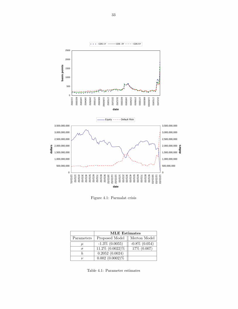
33
0
500,000,000
1,000,000,000
1,500,000,000
2,000,000,000
2,500,000,000
3,000,000,000
3,500,000,000
12/21/011/21/022/21/023/21/024/21/025/21/026/21/027/21/028/21/029/21/0210/21/0211/21/0212/21/021/21/032/21/033/21/034/21/035/21/036/21/037/21/038/21/039/21/0310/21/0311/21/0312/21/03
date
dolla
rs
0
500,000,000
1,000,000,000
1,500,000,000
2,000,000,000
2,500,000,000
3,000,000,000
3,500,000,000
dolla
rs
Equity Default Risk
0
500
1000
1500
2000
2500
1/1/2002
6/2/2002
14/03/02
19/04/02
24/05/02
1/7/2002
6/8/2002
11/9/2002
17/10/02
22/11/02
31/12/02
6/2/2003
14/03/03
21/04/03
27/05/03
1/7/2003
6/8/2003
11/9/2003
17/10/03
21/11/03
date
basi
s po
ints
CDS 1Y CDS 3Y CDS 5Y
Figure 4.1: Parmalat crisis
MLE EstimatesParameters Proposed Model Merton Model
µ -1.3% (0.0055) -0.8% (0.054)σ 11.2% (0.0022)% 17% (0.007)h 0.2052 (0.0024)ν 0.002 (0.0002)%
Table 4.1: Parameter estimates

34
Protection Seller
Protection Buyer
Credit Event Payment
Notional per Spread Premium (bp)
Notional: US $10MMTerm: 5 Years
Figure 4.2: Schematic illustration of a CDS contract
extract an implied probability of fraud of about 0.2. Although there are differences in the assumptions and
analysis between our work and theirs, making it hard to compare, using the simplest version of our model
we find qualitatively similar results to the ones they obtain with the full power of their model.
4.3 Empirical Analysis of Misreporting
We present a statistical analysis of the term structure of the credit default swap curve (CDS) as well as of
the default probabilities bootstrapped from CDS data. Section 4.3.1 briefly recalls the definition of a CDS
instrument. Section 4.3.2 explains the bootstrapped procedure used in implying the default probabilities.
Section 4.3.3 applies the above procedure to three known cases of occurred misreporting and draws inferences
about the information content of those financial instruments in misreporting situations.
4.3.1 CDS Contracts
The credit default swap is the most liquid credit derivative instrument. A CDS is an agreement between two
parties to exchange the credit risk of an issuer called reference entity. The buyer of the CDS pays a periodic
fee to the seller until the maturity of the swap contract or the occurrence of the default event (whichever
comes earlier). The seller of the CDS faces the obligation, until maturity of the swap, to pay the losses
incurred by the protection buyer as a result of the credit event. Such credit event can be bankruptcy, failing
to pay outstanding debt obligations, etc. A schematic illustration of a CDS contract is reported in Figure
4.2.
When a credit event occurs, the protection seller has to make up for losses on general exposures to the
name under the contract. There are several settlement agreements between the buyer and seller on how
to deal with the occurred credit event. The most popular is physical delivery. Under this agreement the
protection buyer is allowed to deliver whatever debt obligation issued by the name and typically the natural

35
choice is to deliver the cheapest one.
We next describe the payments of buyer and seller. For simplicity, we assume that payments occur at
the end of the each period. The payment from the protection seller at the end of any coupon period (time
ti) can be represented as
1ti−1≤ς≤tiLGD (4.3.1)
where 1ti−1 is the indicator function taking value 1 if default occurs between time ti−1 and time ti, while
LGD is the loss given default paid by the protection seller to the protection buyer at the occurrence of the
default event. At time ti the protection buyer will pay instead
s1ς>ti−1 (4.3.2)
i.e, the premium s conditional on the reference entity having survived up to time ti−1. It is assumed that if
the name defaults in a period the contract ends in that period.
We next explain how to evaluate the payments of buyer and seller. Denote Q(t) = P (ς > t) the survival
probability of the issuer up to time t under the risk-neutral measure. The present value of the payment done
at time ti by the protection seller is obtained by taking the expectation of the risky cash flow in Eq. (4.3.1).
Using simple survival analysis, it is easily seen that this is given by
e−r(t−ti)[Q(ti−1)−Q(ti)]LGD (4.3.3)
where [Q(ti−1) − Q(ti)] is the probability of a default event occurring between ti−1 and ti, in which case
the protection seller will have to pay the promised LGD. By a similar argument, the present value of the
payment done by the protection buyer at time ti is
e−r(t−ti)Q(ti−1)s (4.3.4)
where Q(ti−1) is the probability that no default event has occurred before ti−1, in which case the protection
buyer will have to pay the premium s at time ti. The running premium s is the break-even value, i.e.,
the value which makes the present value of the protection buyer cash-flow equal to the present value of the
protection seller cash-flow. For a n-year CDS contract, which thus consists of n payment periods, the spread
s, as seen at time t, will have to satisfy the following equation
n∑i=1
e−r(ti−t)Q(ti−1)s =n∑i=1
e−r(ti−t)[Q(ti−1)−Q(ti)]LGD (4.3.5)
4.3.2 CDS-Implied Default Probabilities
The CDS instruments allow to investigate the term structure of the default probability for the case of obligors
on which CDS contracts are quoted for several maturities. In this case, it is possible to bootstrap the term

36
structure of the default probability in a very similar manner to that by which we usually back out the zero-
coupon factor curve from swap rates. More precisely, assume that a CDS spread s1 is quoted for protection
over a one year horizon. For the sake of simplicity, assume that the spread is paid in one instance at the end
of the year, and it is paid even if the name has defaulted. Moreover, assume that before time t1 no default
has occurred yet. Using Eq. (4.3.5) with n = 1, we obtain
s1 = [1−Q(t1)]LGD (4.3.6)
from which we can immediately imply
Q(t1) = 1− s1LGD
(4.3.7)
The value for Q(t1) can then be plugged into Eq. (4.3.5) applied to a 2 year CDS contract, thus obtaining
2∑i=1
e−r(ti−t)Q(ti−1)s2 =2∑i=1
e−r(ti−t)[Q(ti−1)−Q(ti)]LGD (4.3.8)
from which we can back out Q(t2), since we have Q(t1) and s2 which is the 2 year CDS quote observed on the
market. We can continue iterating this process until extracting the survival probabilities for all maturities.
4.3.3 Signals of Misreporting Inferred from CDS
We report the results of an empirical investigation which evidences the impact of misreporting and financial
distress on the term structure of the CDS curve and the resulting bootstrapped default probabilities. We
found that the misreporting event is typically announced by an inversion of the term structure of the CDS
spread curve. We next report the results of this analysis on three major cases of misreporting in United
States history, namely on Enron, WorldCom, and Tyco, and make some comments about them. We start
presenting the results for the Tyco case. On March 13, 2001, Tyco announced a 9.2 billion cash and stock
deal to take over the CIT group, a commercial finance company. This CIT deal led to sudden discovery of
management misconduct. Tyco shares dropped sharply at the end of January 2002, as a proxy report was
filed with the Securities and Exchange Commission disclosing that the Tyco CFO received a 10 million fee
on conclusion of the CIT Group deal, and that another $10 million went to a charity where he was a director.
The crisis at the end of January 2002 is evidenced very clearly from Figures 4.3 and 4.4. The shape of the
term structure curve was inverted, so that the 3 year CDS contract was quoting on average about 100 basis
points (bps) less than the 1 year contract, and the 5 year contract was quoting about 190 bps lower. The
inverted shape persisted across all of year 2002 and was only reversed in late 2003. An inverted structure
of the CDS spread is indeed typical of periods of particular financial distress. This means that the market
prices a very high probability of default in the first year, while the probability is lower for the years further
in the future. The rational behind is that if the company survives this initial period, then it will be in better
shape and less likely to (conditionally) default over subsequent periods. All this is confirmed from data of
the cumulative default probability which are displayed in Figure 4.4. The 1 year default probability was
about 1.39% on average in the last quarter of 2001; 5 year default probability was about 5 times larger, i.e.,
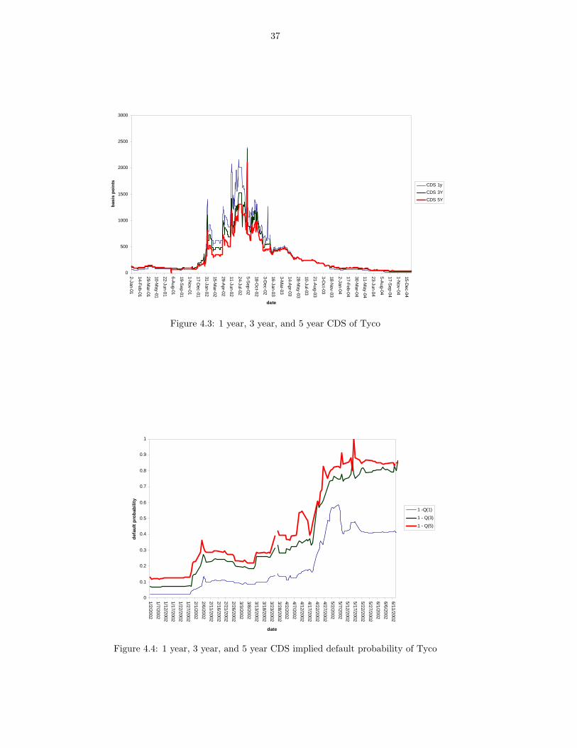
37
0
500
1000
1500
2000
2500
3000
2-Jan-01
14-Feb-01
29-Mar-01
10-May-01
22-Jun-01
6-Aug-01
19-Sep-01
1-Nov-01
17-Dec-01
31-Jan-02
15-Mar-02
29-Apr-02
11-Jun-02
24-Jul-02
5-Sep-02
18-Oct-02
3-Dec-02
16-Jan-03
3-Mar-03
14-Apr-03
28-May-03
10-Jul-03
21-Aug-03
3-Oct-03
18-Nov-03
2-Jan-04
17-Feb-04
30-Mar-04
11-May-04
23-Jun-04
5-Aug-04
17-Sep-04
1-Nov-04
15-Dec-04
date
basi
s po
ints CDS 1y
CDS 3YCDS 5Y
Figure 4.3: 1 year, 3 year, and 5 year CDS of Tyco
0
0.1
0.2
0.3
0.4
0.5
0.6
0.7
0.8
0.9
1
1/2/20021/7/20021/12/20021/17/20021/22/20021/27/20022/1/20022/6/20022/11/20022/16/20022/21/20022/26/20023/3/20023/8/20023/13/20023/18/20023/23/20023/28/20024/2/20024/7/20024/12/20024/17/20024/22/20024/27/20025/2/20025/7/20025/12/20025/17/20025/22/20025/27/20026/1/20026/6/20026/11/2002
date
defa
ult p
roba
bilit
y
1 -Q(1)
1 - Q(3)
1 - Q(5)
Figure 4.4: 1 year, 3 year, and 5 year CDS implied default probability of Tyco

38
0
500
1000
1500
2000
2500
3000
3500
4000
1/2/2002
1/7/2002
1/12/2002
1/17/2002
1/22/2002
1/27/2002
2/1/2002
2/6/2002
2/11/2002
2/16/2002
2/21/2002
2/26/2002
3/3/2002
3/8/2002
3/13/2002
3/18/2002
3/23/2002
3/28/2002
4/2/2002
4/7/2002
4/12/2002
4/17/2002
4/22/2002
4/27/2002
5/2/2002
5/7/2002
5/12/2002
5/17/2002
5/22/2002
5/27/2002
6/1/2002
6/6/2002
6/11/2002
date
basi
s po
ints
CDS 1YCDS 3YCDS 5Y
Figure 4.5: 1 year, 3 year, and 5 year CDS of WorldCom
7.51%. This means that the market was attributing good financial health to the firm and was not suspecting
fraud. In the first quarter of 2004, the 1 year default probability climbed to 9.56%, while the 5 year default
probability grew up to 22.90%. Since the 3 year default probability was 21%, thus very close to the 5 year
default probability, the market was implying a probability of default between years 2005 and 2007 of about
1.90%. This is close to the 1 year default probability in the pre-crisis situation, meaning that the market
was believing that either the company would have defaulted three years from now, or not defaulted at all.
We next report the same figures for WorldCom, the biggest corporate bankruptcy in the history of the
United States. WorldCom was a giant leading the telecommunication industry at the end of last century
and was handling 50% of the US internet traffic and 50% of e-mail worldwide. The fraud began when it
was discovered that the former chief financial officer at WorldCom had directed employees to falsify balance
sheets to hide more than $3.8 billion of expenses. The fraud was discovered in March 2002, when the internal
audit found accounting irregularities consisting of $400 million that had been set aside to boost WorldCom’s
income. After asking for documents supporting capital expenditures and discovering that no supporting
accounting standards existed, the Internal audit explained irregularities to the Audit Committee on June
20, 2002, and on July 21, 2002, WorldCom filed for bankruptcy.
Figure 4.5 reports the CDS term structure in the year of crisis. The CDS spreads climbed up about at
the same time as the Tyco crisis. At the end of the January, the spreads increased substantially, and the
term structure of the spread became inverted. Two months later, the 1 year CDS quoted 608 basis points
on average, and the 3 and 5 year maturities respectively quoted 147 and 194 basis points less than that.
Again, this corresponds to a massive increase of the default probability in the first year horizon that does
not seem to spread out to the following years. In January, the average 1 year default probability was 2.30%,
the 3 year default probability was 6.30%, and the 5 year default probability was 12.60%. In the following
two months the crisis caused an increase of the 1 year default probability to more than 10%, while the 3

39
0
0.1
0.2
0.3
0.4
0.5
0.6
0.7
0.8
0.9
1
1/2/20021/7/20021/12/20021/17/20021/22/20021/27/20022/1/20022/6/20022/11/20022/16/20022/21/20022/26/20023/3/20023/8/20023/13/20023/18/20023/23/20023/28/20024/2/20024/7/20024/12/20024/17/20024/22/20024/27/20025/2/20025/7/20025/12/20025/17/20025/22/20025/27/20026/1/20026/6/20026/11/2002
date
defa
ult p
roba
bilit
y
1 -Q(1)
1 - Q(3)
1 - Q(5)
Figure 4.6: 1 year, 3 year, and 5 year CDS implied default probability of WorldCom
and 5 year default probability climbed to 22.66% and 27.95%, respectively. From this, it can be implied
that the implied probability of defaulting between third and fifth year was about 5.30%, even less than in
the pre-crisis period. Again the market was believing that, if had the company had defaulted, it would have
done so in the next three years. This is confirmed from facts since WorldCom was only part of stock market
history three years later.
We conclude this empirical investigation with the well-known Enron case, a large player in the natural
gas and energy supply. Enron was raising off balance sheet debt by resorting to almost a thousand special
purpose entities funded by banks and outside investors. This practice allowed Enron to exploit a loophole in
the US Generally Accepted Accounting Standard (US GAAP) to circumvent the principle of consolidation.
Under the GAAP, the balance sheet of a special purpose entity needs not be consolidated with the originator
if two conditions hold: outside investors must supply at least 3% of the funds, and the originator cannot
control the disposition of the assets under control of the entity. This technique enables increasing leverage
in the assets of Enron, without reporting this stock of debt in the company accounting data. This leverage
effect boosted growth of the company when the fundamentals of its business were good, but by the same
token accelerated the crisis when the market turned against Enron, which happened between 2000 and 2001.
Signals of crisis began on October 17, 2001, when Enron announced a downward revision of its third
quarter results by more than 1 billion dollars, mainly due to investment losses. This triggered a series
of events leading to Moody’s downgrading of Enron credit to junk and the subsequent filing of Enron for
Chapter 11 which occurred on December 2, 2001.
Even in this case the crisis was announced by the inversion of the CDS spread term structure, which
took place in mid-October 2001 when the first signals of crisis started appearing. It was the first time
when inversion of the CDS term structure took place, and the one year CDS climbed higher than 500 basis
points. The 1 year default probability remained between 1.6% and 2.4%, the 3 year default probability

40
0
500
1000
1500
2000
2500
3000
3500
4000
4500
1/15/2001
1/29/2001
2/12/2001
2/26/2001
3/12/2001
3/26/2001
4/9/2001
4/23/2001
5/7/2001
5/21/2001
6/4/2001
6/18/2001
7/2/2001
7/16/2001
7/30/2001
8/13/2001
8/27/2001
9/10/2001
9/24/2001
10/8/2001
10/22/2001
11/5/2001
11/19/2001
date
basi
s po
ints CDS 1Y
CDS 3YCDS 5Y
Figure 4.7: 1 year, 3 year, and 5 year CDS of Enron
0
0.1
0.2
0.3
0.4
0.5
0.6
0.7
0.8
1/16/2001
1/26/20012/5/2001
2/15/20012/25/2001
3/7/20013/17/2001
3/27/20014/6/2001
4/16/20014/26/2001
5/6/2001
5/16/20015/26/2001
6/5/20016/15/2001
6/25/20017/5/2001
7/15/20017/25/2001
8/4/20018/14/2001
8/24/2001
9/3/20019/13/2001
9/23/200110/3/2001
10/13/200110/23/2001
11/2/200111/12/2001
11/22/2001
date
Def
ault
prob
abili
ty
1-Q(1)
1-Q(3)
1-Q(5)
Figure 4.8: 1 year, 3 year, and 5 year CDS implied default probability of Enron

41
stayed between 6% and 8%, and the 5 year default probability between 10% and 12%. This means that the
probability of defaulting between three and five year from that time was roughly 4%. On the day of the crisis,
October 22nd, the one year default probability climbed to 8.47%, the 3 year default probability jumped to
20.8% and the 5 year one jumped to 24.94%, thus without any increase on the probability of defaulting
between 3 and 5 years from now. Again, the market was believing that if the company had defaulted, it
would have done so in the next three years. This was actually the case, since Enron did not manage to
survive until the end of the year.
Hence, this empirical investigation showed that cases of misreporting have similarities. They all manifest
a steepness of the credit spread curve, with short maturity spreads getting larger than long maturity spread.
They all exhibit an increase of the probability of defaulting in the short term, leaving the probability of
defaulting in the next years roughly the same as in the pre-crisis situation.

42
Chapter 5
Stochastic Filtering For JumpSystems
This chapter is devoted to the presentation of an approximate filtering scheme used to compute the filtering
density needed for pricing securities of our credit model in Chapter 3.
We recall, from the previous chapter, that the system presented in Eq. (3.3.1–3.3.4) is a jump linear
system with state dependent transition probabilities. Even if an analytical expression for the optimal filtering
density may be provided (see Section 5.2), it turns out to be computationally prohibitive to evaluate the
density on a given input. To this purpose, we develop an approximation method, which allows evaluating
the conditional density of a given state in polynomial time. Although the filtering problem associated with
our credit risk model given in Eq. (3.3) is one dimensional, we study the filtering problem in the multi-
dimensional case, namely allowing both the state and the observation to be n-dimensional vectors. When
both the state and the observation are scalar, the developed procedure would return the filtering density
used to price bonds in Eq. (3.4.14) and equity in Eq. (3.4.15).
The output of the proposed scheme is an approximation of the true unnormalized posterior density
with a mixture of Gaussian densities. Such densities are selected as the solution of a convex programming
problem aiming at finding the sparsest possible expansion in terms of Gaussian densities, which is as close
as possible to the actual unnormalized density. Our proposed scheme is validated on both theoretical and
empirical grounds. From a theoretical point of view, we provide an upper bound on the total variation
distance between the true filter density and the approximation density returned from our scheme. Such
upper bound may be on-line computed using the system parameters, the received observations, and the
constraints imposed on the convex optimization problem, without any recourse to Monte-Carlo simulations.
Therefore, the developed bound would allow the user efficiently control the propagation of the approximation
error introduced by the method over time. On empirical grounds, we compare the proposed method to the
IMM and GPB2 estimators of Bar-Shalom et al. (2002), two widely used heuristic procedures used to deal
with Markovian jump systems. We show that the estimation quality is superior at the expenses of an increase
in computational burden, which tends to be a bottleneck for high-dimensional state space systems. This
happens because the proposed method is based on a gridding of the state space and has complexity growing
exponentially with the size of the state space. However, this is not a major concern for us since the state
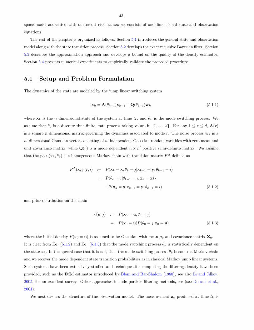
43
space model associated with our credit risk framework consists of one-dimensional state and observation
equations.
The rest of the chapter is organized as follows. Section 5.1 introduces the general state and observation
model along with the state transition process. Section 5.2 develops the exact recursive Bayesian filter. Section
5.3 describes the approximation approach and develops a bound on the quality of the density estimator.
Section 5.4 presents numerical experiments to empirically validate the proposed procedure.
5.1 Setup and Problem Formulation
The dynamics of the state are modeled by the jump linear switching system
xk = A(θk−1)xk−1 + Q(θk−1)wk (5.1.1)
where xk is the n dimensional state of the system at time tk, and θk is the mode switching process. We
assume that θk is a discrete time finite state process taking values in 1, . . . , d. For any 1 ≤ r ≤ d, A(r)
is a square n dimensional matrix governing the dynamics associated to mode r. The noise process wk is a
n′ dimensional Gaussian vector consisting of n′ independent Gaussian random variables with zero mean and
unit covariance matrix, while Q(r) is a mode dependent n × n′ positive semi-definite matrix. We assume
that the pair (xk, θk) is a homogeneous Markov chain with transition matrix P∆ defined as
P∆(x, j,y, i) := P (xk = x, θk = j|xk−1 = y, θk−1 = i)
= P (θk = j|θk−1 = i,xk = x) ·
· P (xk = x|xk−1 = y, θk−1 = i) (5.1.2)
and prior distribution on the chain
π(u, j) := P (x0 = u, θ0 = j)
= P (x0 = u)P (θ0 = j|x0 = u) (5.1.3)
where the initial density P (x0 = u) is assumed to be Gaussian with mean µ0 and covariance matrix Σ0.
It is clear from Eq. (5.1.2) and Eq. (5.1.3) that the mode switching process θk is statistically dependent on
the state xk. In the special case that it is not, then the mode switching process θk becomes a Markov chain
and we recover the mode dependent state transition probabilities as in classical Markov jump linear systems.
Such systems have been extensively studied and techniques for computing the filtering density have been
provided, such as the IMM estimator introduced by Blom and Bar-Shalom (1988), see also Li and Jilkov,
2005, for an excellent survey. Other approaches include particle filtering methods, see (see Doucet et al.,
2001).
We next discuss the structure of the observation model. The measurement zk produced at time tk is
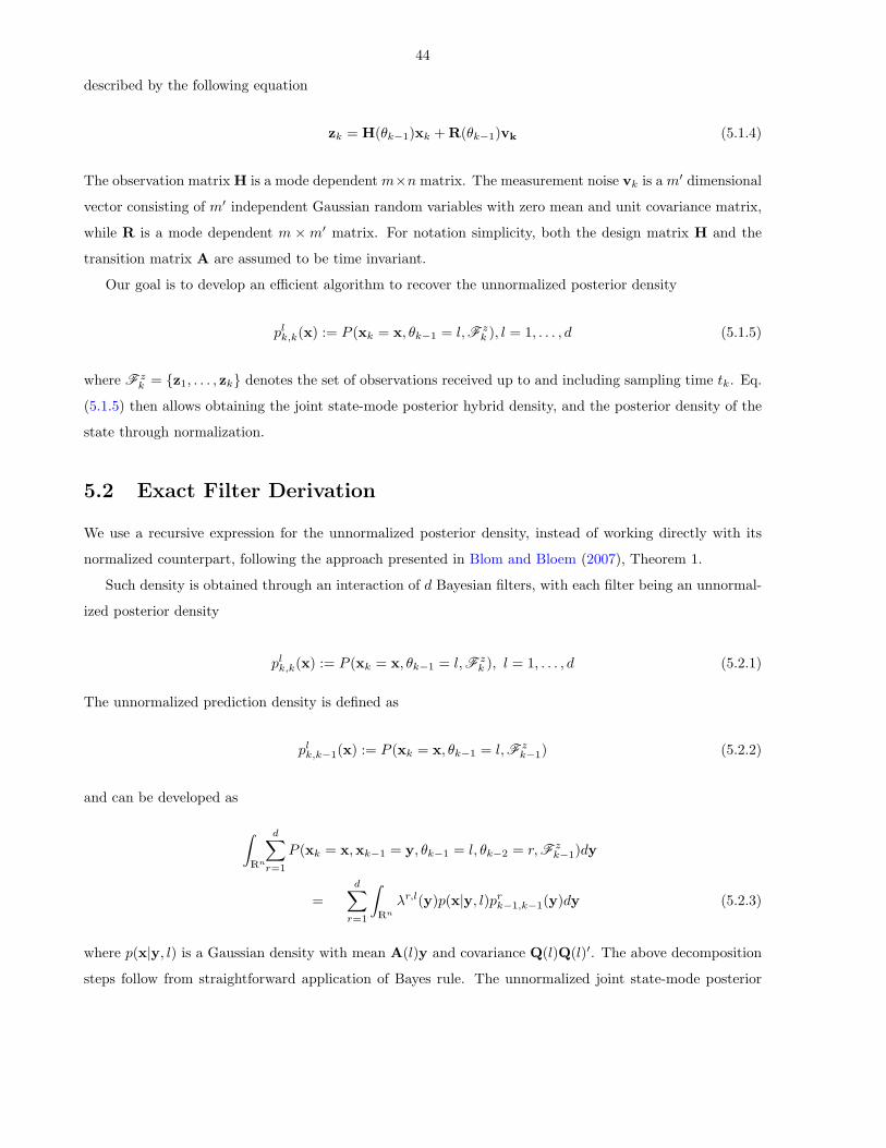
44
described by the following equation
zk = H(θk−1)xk + R(θk−1)vk (5.1.4)
The observation matrix H is a mode dependent m×n matrix. The measurement noise vk is a m′ dimensional
vector consisting of m′ independent Gaussian random variables with zero mean and unit covariance matrix,
while R is a mode dependent m ×m′ matrix. For notation simplicity, both the design matrix H and the
transition matrix A are assumed to be time invariant.
Our goal is to develop an efficient algorithm to recover the unnormalized posterior density
plk,k(x) := P (xk = x, θk−1 = l,F zk ), l = 1, . . . , d (5.1.5)
where F zk = z1, . . . , zk denotes the set of observations received up to and including sampling time tk. Eq.
(5.1.5) then allows obtaining the joint state-mode posterior hybrid density, and the posterior density of the
state through normalization.
5.2 Exact Filter Derivation
We use a recursive expression for the unnormalized posterior density, instead of working directly with its
normalized counterpart, following the approach presented in Blom and Bloem (2007), Theorem 1.
Such density is obtained through an interaction of d Bayesian filters, with each filter being an unnormal-
ized posterior density
plk,k(x) := P (xk = x, θk−1 = l,F zk ), l = 1, . . . , d (5.2.1)
The unnormalized prediction density is defined as
plk,k−1(x) := P (xk = x, θk−1 = l,F zk−1) (5.2.2)
and can be developed as
∫Rn
d∑r=1
P (xk = x,xk−1 = y, θk−1 = l, θk−2 = r,F zk−1)dy
=d∑r=1
∫Rn
λr,l(y)p(x|y, l)prk−1,k−1(y)dy (5.2.3)
where p(x|y, l) is a Gaussian density with mean A(l)y and covariance Q(l)Q(l)′. The above decomposition
steps follow from straightforward application of Bayes rule. The unnormalized joint state-mode posterior

45
density may then be obtained as
plk,k(x) = Llk|k(x)plk,k−1(x) k ≥ 2
pl1,1(x) = Ll1|1(x)∫Rn p(x|u, l)π(u, l)p(u)du
(5.2.4)
where the correction term Llk|k(x) is a Gaussian density with mean H(l)x and covariance R(l)R(l)′ due to
the structure of the observation equation (5.1.4).
From the above derivations, we can see that the filters interact with each other according to fundamental
Bayesian rules, leading to the recursive expression given in Eq. (5.2.4) for the unnormalized density. It is
important to notice that such recursion is linear. The linearity of the recursion allows provision of an upper
bound for the error committed by our method at any sampling time tk.
The posterior density may then be obtained from the interacting bayesian filters through normalization
as
pk|k(x) =
∑dl=1 p
lk,k(x)∫
Rn
∑dl=1 p
lk,k(x)dx
(5.2.5)
5.3 The Filter Approximation Scheme
The filter described in Section 5.2 cannot be implemented efficiently. First of all, the recursive expression
(5.2.4) shows that an exponentially increasing number of filters have to interact to obtain the unnormalized
density at time tk. Additionally, Eq. (5.2.3) involves the evaluation of non-Gaussian integrals due to the
appearance of the terms λj,l(y) in plk,k−1(x), and such integrals are computationally expensive to evaluate.
Furthermore, the normalization step required to obtain the posterior density in Eq. (5.2.5) involves an
evaluation of d spatial integrations, thus increasing the computational burden even further. In order to
deal with these computational issues, we propose an approach which at every step k approximates the
unnormalized density using a restricted set of Gaussian densities, selected from a prescribed base set. The
number of densities and the weight of each density are recovered as the solution of a convex second-order
cone programming problem.
5.3.1 The Approximation Method
Let p(x) be the density which we wish to approximate. Let I and J be two set of indices. We construct a
base set of multivariate Gaussian densities
B = ni,j(x)i∈I,j∈J (5.3.1)
where ni,j(x) stands for the multivariate Gaussian density with mean µi and covariance Σj . Moreover, we
require
µi1 6= µi2 , ∀i1 6= i2
Σj1 6= Σj2 ∀j1 6= j2 (5.3.2)

46
meaning that the means and the covariances of the Gaussian densities in B are all different. We choose a
training set
X = (x1,x2, . . . ,xq) (5.3.3)
of size q containing vectors in Rn. Let us define the matrix
Φ(X) =
n1(x1) n2(x1) . . . n|I|(x1)
n1(x2) n2(x2) . . . n|I|(x2)...
.... . .
...
n1(xq) n2(xq) . . . n|I|(xq)
(5.3.4)
where ni(xl) = (ni,1(xl), ni,2(xl), . . . , ni,|J|(xl)), i.e., a row vector whose j-th entry is the multivariate
Gaussian density in B with mean µi and covariance Σj evaluated at xl.
Moreover, we assume that q < |I| × |J |, i.e., the size of the training set, is strictly smaller than the
cardinality of the base set B. Let p = (p(x1), . . . , p(xq))′. The linear system
p = Φz (5.3.5)
is solvable and overdetermined being q < |I|×|J |. Although we could solve the system and then approximate
the density p(x) with φz(x), we notice that such approach would require propagating a number of Gaussian
densities equal to the size q of the training set, and therefore it would scale linearly with the size of the
training set, making a real time implementation computationally intensive. Our goal is to approximate
p using a short linear combination of Gaussian densities and at the same time minimize the introduced
approximation error. Therefore, we look for the sparsest representation of p(x) in the following sense:
min ||υ||0 subject to ||p−Φυ||2 ≤ ι (P1)
(P1) is a mathematical programming problem with decision variables υ, and ||υ||0 denotes the number of
nonzero entries of the vector υ, i.e.,
||υ||0 = |(i, j) : υ(i,j) 6= 0| (5.3.6)
where υ(i,j) is the entry of the |I| × |J | dimensional vector υ multiplying the Gaussian density ni,j . If υ∗
is the solution of (P1), we would approximate p(x) with φυ∗(x). However, this is of little practical use,
since (P1) is non-convex and easy to solve only in the special case when the system p = Φυ admits a
unique solution (see Donoho and Elad, 2003). In all other cases, its solution usually requires an intractable
combinatorial search. In order to overcome this computational burden, basis pursuit (see Chen et al., 2001)
has become the most widely used numerical shortcut to approximate the solution to (P1). Such method
replaces the l0 norm with its closest convex penalty function, the l1 norm, and solves

47
min ||$||1 subject to ||p−Φ$||2 ≤ ε (P2)
with decision variable $. The problems (P1) and (P2) differ only in the choice of the objective function,
with the latter using an l1 norm as a proxy for the sparsity count. However, unlike (P1), (P2) is a convex
second-order cone programming problem. This can be seen by rewriting the problem (P2) in the following
form
min1Tu subject to− u ≤ $ ≤ u ||p−Φ$||2 ≤ ε (P3)
where we added the slack optimization variable u. In the above formulation 1 is a vector of ones and the
vector inequality $ ≤ u means component-wise, i.e., wi ≤ ui for all i. Being a convex programming problem,
(P2) can be solved efficiently using standard optimization algorithms. Therefore, we will approximate the
actual density p as
p(x) ≈ Φ$(x) (5.3.7)
5.3.2 Sparsity of the approximation
In this section, we discuss the relation between the approximation errors ι and ε resulting from the solution
of problems (P1) and (P2) and the sparsity of the corresponding solutions. Let Λ ⊆ I × J denote a generic
subset. We define the inner product between two vectors as their dot product, i.e.,
< x,y >=∑i
xiyi (5.3.8)
and denote by
ni,j(X) = (ni,j(x1), ni,j(x2), . . . , ni,j(xq)) (5.3.9)
the vector obtained evaluating the Gaussian density ni,j at all points of the training set X. We define the
cumulative coherence as
c(s) = max|Λ|=s
max(i,j)/∈Λ
∑(u,v)∈Λ
| < ni,j(X), nu,v(X) > | (5.3.10)
which measures how much a collection of fixed densities resembles a fixed, distinct density, with the con-
vention that c(0) = 0. The maximum correlation of the density vector p with the set of base densities B is
defined as
maxcor(p) = max(i,j)∈I×J
| < p, ni,j(X) > |||p||2
(5.3.11)
We now report the following result from citetTropprelax, as:
Lemma 5.1. Let aopt = Φυ∗ where υ∗ is an optimal solution to the mathematical programming problem
(P1) with tolerance ι. If ||υ∗||0 = s, and c(s) ≤ 13 , and we select
ε ≥ ι√
1 + 6s maxcor(p− aopt)2 (5.3.12)

48
then the solution $∗ to (P2) with tolerance ε is at least as sparse as the solution υ∗, i.e.,
||$∗||0 ≤ ||υ∗||0 (5.3.13)
In words, the above lemma states that if our base set B has a sufficiently high degree of independence,
namely, c(s) ≤ 13 , then we do not lose sparsity by using the l1 norm instead of the l0 norm in the programming
problem, although this happens at the expenses of an increase in the approximation error ε which will depend
upon the sparsity of the solution of (P1) and the correlation of the residual of (p− aopt) with the base set
B.
5.3.3 The Filter Approximation
We describe how to construct an approximation to the actual unnormalized density plk,k(x) at time tk from
an existing set of approximations to the unnormalized density prk−1,k−1(y)r=1,...,d available from time tk−1.
For any r = 1, . . . , d, let us denote by prk−1,k−1(y) such an approximation which would have been computed
in the previous step of the approximation procedure. Let
Ωlk = (i, j) ∈ I × J : [$lk](i,j) 6= 0 (5.3.14)
where $lk is the solution of (P2) obtained when approximating plk,k(x), i.e.,
prk−1,k−1(y) ≈∑
(i,j)∈Ωrk−1
[$rk−1](i,j)ni,j(y) (5.3.15)
In Eq. (5.3.15), we want to highlight that we are only propagating from time tk−1 to time tk the Gaussian
densities in B with nonzero weight. Our goal is to approximate the actual filter density plk,k(x) at time tk
given by Eq. (5.2.4). This is done in two separate steps. The output of the first step is an approximate
density plk,k(x) computed as follows:
plk,k(x) := Llk|k(x)d∑r=1
∫Rn
λr,l(y)p(x|y, l)prk−1,k−1(y)dy (5.3.16)
≈ Llk|k(x)d∑r=1
∫Rn
λr,l(y)p(x|y, l)prk−1,k−1(y)dy
= plk,k(x)
where the approximation step consists in replacing each term prk−1,k−1(y) with its previously computed
approximation prk−1,k−1(y). Plugging Eq. (5.3.15) into Eq. (5.3.17), we obtain
plk,k(x) = Llk|k(x)d∑r=1
∑(i,j)∈Ωr
k−1
[$rk−1](i,j)
·∫Rn
λr,l(y)p(x|y, l)ni,j(y)dy (5.3.17)

49
Eq. (5.3.17) shows that we have obtained an approximation density plk,k(x) for plk,k(x) consisting of
·∑dr=1 |Ωrk−1| components. Moreover, plk,k(x) is no longer a mixture of Gaussians due to the appearance of
the state-dependent mode transition term λr,l(y). To this purpose, we approximate plk,k(x) further before
propagating it to the next step sampling time tk+1. This is the second step of our methodology, which is
described next. We first compute the mean and standard deviation of the unnormalized density plk,k(x).
These can be efficiently computed by rewriting the integral as a sum of expectations, each one taken with
respect to two independent random variables, one being a Gaussian and another being a Gaussian mixture.
For computing the mean, we proceed as follows:
xlk,k =∫Rn
plk,k(x)xdx
=d∑r=1
||$rk−1]||1EX,Yr [xL
lk|k(x) λr,l(y)] (5.3.18)
where X and Yr are dependent vectors from which samples are drawn as follows. We first sample y from
Yr according to the Gaussian mixture distribution with density given by
Yr ∼∑
(i,j)∈Ωrk−1
[$rk−1](i,j)
||$rk−1||1
ni,j(y) (5.3.19)
We next sample x from a Gaussian distribution with density given by
X ∼ n(x;A(l)y,Q(l)) (5.3.20)
Monte-Carlo methods can be applied to efficiently approximate the above expectation. A similar argument
can be followed to approximate the covariance matrix of plk,k(x), let us call it Σlk,k. We then choose an
n-dimensional ellipsoid G ∈ Rn defined as
(x− xlk,k)′(Σl
k,k)−1(x− xlk,k) (5.3.21)
Both the training points in X and the means of the Gaussian densities in B are selected to be on an equally
spaced grid covering the ellipsoid G. The covariances of the densities in B are defined by specifying the
standard deviation of each state space component σi, i ∈ 1, . . . n, and the correlation factors between them,
ρi,j , i, j ∈ 1, . . . , n. For each covariance matrix, σi = σ, i.e., the standard deviation is assumed to be the
same for each component. The σ values decay exponentially from σmax to σmin to capture the behavior of
the Gaussian density which exhibits exponential tails. The correlation factors ρi,j are equally spaced in the
interval (−1, 1). We next evaluate the density plk,k(x) on the points in X, thus obtaining a vector
plk,k = (plk,k(x1), . . . , plk,k(xq)) (5.3.22)
Let εlk be the smallest component of the vector plk,k. Then we solve the optimization problem (P2) as follows:

50
Previous unnormalized posterior pdfs mkkkk pp 1,1
11,1 ˆ,...,ˆ −−−−
AGGREGATION-APPROXIMATION
APPROXIMATION USING L1 NORM METHOD
… FILTERFm
FILTERF1
Updated unnormalized posterior pdfs mkkkk pp ,
1, ,..., ((
meas. mode θ1
kz meas. mode θm
kz
New gaussian mixture approximations for mkkkk pp ,
1, ˆ,...,ˆ
Figure 5.1: One cycle of the estimator
min ||$lk||1 subject to ||plk,k −Φ$l
k||2 ≤ εlk (P4)
If $l,∗k denotes the optimal solution to (P4), the approximation density propagated to step k + 1 is
plk,k(x) =∑
(i,j)∈Ωlk
[$l,∗k ](i,j)ni,j(x) (5.3.23)
We summarize the whole procedure with a block diagram of the estimator in Figure 5.1. It is clear from
Figure 5.1 that the mode conditional densities are approximated right after the mixing step.
5.3.4 Distance between Approximate and Optimal Filter
We provide an upper bound on the total variation distance between the actual density plk,k(x) and the
approximate density plk,k(x) obtained using our method. Let us denote
plk,k(x) := plk,k(x)− plk,k(x) (5.3.24)
The total variation distance between plk,k(x) and plk,k(x) is defined as
||plk,k||1 :=∫Rn
|plk,k(x)|dx (5.3.25)
Let ρ be the distance between two vectors in the training set X. If those vectors are chosen using the
methodology described in Section 5.3.3, it is reasonable to assume that
plk,k(y) ≈ 0,y /∈ G (5.3.26)
In words, plk,k(x) concentrates most of its probability mass inside X.

51
Since our approximation scheme finds the sparsest possible approximation of the density with a guaran-
teed error bound ε, the mass of the approximate density plk,k(x) recovered by (P2) would also be negligible
on the region Rn−G. This is because the selection of any Gaussian component whose mean lies outside the
grid would increase the l1 norm of the optimal weight vector without reducing the approximation error any
further since the training set does not contain any vector outside the grid. Therefore, the recovered solution
would not be optimal. This justifies the following approximation for the l1 norm
||plk,k||1 ≈∫G
|plk,k(x)|dx (5.3.27)
We next state the final result under the form of two theorems, one for the density approximation at initial
time, and one for the approximation at a generic sampling time. The detailed proofs are reported in Appendix
G and H, respectively.
Define
C(l) = supx∈Rn
||∇Llk|k(x)||∞(2π)
n2 det(Q(l))
12
+ supx∈Rn
||∇p(x|y, l)||∞(2π)
m2 det(R(l))
12
(5.3.28)
where
∇Llk|k(x) = −e− 1
2 (zk−H(l)x)′R(l)−1(zk−H(l)x)
(2π)m2 det(R(l))
12
· R(l)−1(zk −H(l)x)
∇p(x|y, l) = −e− 1
2 (x−A(l)y)′Q(l)−1(x−A(l)y)
(2π)n2 det(Q(l))
12
· Q(l)−1(x−A(l)y)
(5.3.29)
Notice that Llk|k(x) is independent of the time step k due to the time invariant assumption on the design
matrix H made in Section 5.1. Let
Ck = sup(j,h)∈Ωl
k
supx∈Rn
||∇nj,h(x)||∞ (5.3.30)
and recall that $l,∗k is the optimal solution recovered when using (P4) to approximate plk,k(x).
Theorem 5.1. The total variation distance between the actual density and the approximation density at t1
is
||pl1,1||1 ≤ q(el,21 + el,31 + el,41 ) ∀l = 1, . . . , d (5.3.31)
whereel,21 := 1
2C(l)nρn+1En(µ0,Σ0)[λ
l]
el,31 := εl1ρn
el,41 := C1nρn+1 · ||$l,∗
1 ||1
(5.3.32)
Let us denote by S(l) = HQ(l)HT +R(l) the mode conditioned measurement prediction covariance matrix.
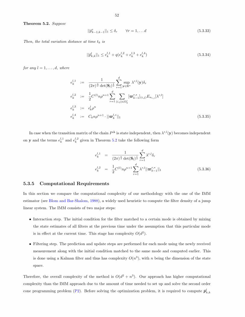
52
Theorem 5.2. Suppose
||prk−1,k−1||1 ≤ δr ∀r = 1, . . . d (5.3.33)
Then, the total variation distance at time tk is
||plk,k||1 ≤ el,1k + q(el,2k + el,3k + el,4k ) (5.3.34)
for any l = 1, . . . , d, where
el,1k :=1
(2π)n2 det(Sl)
12
d∑r=1
supy∈Rn
λr,l(y)δr
el,2k :=12C(l)nρn+1
d∑r=1
∑(i,j)∈Ωr
k
[$r,∗k−1](i,j)Eni,j [λ
r,l]
el,3k := εlkρn
el,4k := Cknρn+1 · ||$l,∗
k ||1 (5.3.35)
In case when the transition matrix of the chain P∆ is state independent, then λr,l(y) becomes independent
on y and the terms el,1k and el,2k given in Theorem 5.2 take the following form
el,1k =1
(2π)n2 det(Sl)
12
d∑r=1
λr,lδr
el,2k =12C(l)nρn+1
d∑r=1
λr,l||$r,∗k−1||1 (5.3.36)
5.3.5 Computational Requirements
In this section we compare the computational complexity of our methodology with the one of the IMM
estimator (see Blom and Bar-Shalom, 1988), a widely used heuristic to compute the filter density of a jump
linear system. The IMM consists of two major steps:
• Interaction step. The initial condition for the filter matched to a certain mode is obtained by mixing
the state estimates of all filters at the previous time under the assumption that this particular mode
is in effect at the current time. This stage has complexity O(d2).
• Filtering step. The prediction and update steps are performed for each mode using the newly received
measurement along with the initial condition matched to the same mode and computed earlier. This
is done using a Kalman filter and thus has complexity O(n3), with n being the dimension of the state
space.
Therefore, the overall complexity of the method is O(d2 + n3). Our approach has higher computational
complexity than the IMM approach due to the amount of time needed to set up and solve the second order
cone programming problem (P2). Before solving the optimization problem, it is required to compute plk,k

53
for any mode l and this has complexity O(d2|I||J |q). This is because plk,k(x) in Eq. (5.3.17) may be written
as
plk,k(x) =d∑r=1
∑(i,j)∈Ωl
k
[$rk−1](i,j) Eni,j [L
lk|k(x)λr,l(Yi,j)p(x|Yi,j , l)] (5.3.37)
where Yi,j is a Gaussian random vector with mean µi and covariance Σj . For each x ∈ X in the training
set, it is required to compute d|I||J | Gaussian integrals which can be done in constant time using Hermite
polynomials. This has to be repeated for each mode, thus the total complexity is O(d2q|X||I||J |). Then the
optimization problem needs to be solved for each mode, and this can be done in time O((|I||J |)2q) using the
algorithm proposed by Lobo et al. (1998).
Thus the complexity of the approach grows quadratically with the size of the base set and the number
of modes, and linearly in the size of the training set. This makes the approach slower than the IMM
estimator for high dimensional systems where a larger base set and training set would be required to have
good approximation quality. However, the approach would be very efficient for low-dimensional systems.
5.3.6 Quantitative Evaluation of the TVD
We perform a quantitative evaluation of the total variation distance upper bound derived in Section 5.3.4.
This is done by means of a simple experiment considering a one-dimensional bimodal state space system
defined asxk = xk−1 +Q(l)wk
zk = xk +Rvk(5.3.38)
where wk is a white noise sequence with variance depending on the mode in place at time k, while the
measurement noise vk is assumed to be mode-independent. The two-mode dependent process noises are
zero-mean and only differ in the choice of the standard deviation which is set to Q(1) = 0.7ms2 for mode 1,
and to Q(2) = 4ms2 for mode 2. The standard deviation of the measurement noise is R = 2ms2 . The duration
of each sampling period is 1.5 seconds.
The mode transitions are assumed to be state independent with transition matrix given by
λi,j =
0.6 0.4
0.3 0.7
(5.3.39)
and initial mode distribution given by the vector [0.95, 0.05]. The true trajectory is simulated for 14 sampling
times using a single process noise sequence having standard deviation 0.5ms2 and zero mean for all times except
for the sampling times from k = 3 to k = 7 where
E[w3] = 10ms2 E[w4] = 9ms2 E[w5] = 8ms2
E[w6] = 7ms2 E[w7] = 6ms2
The target is assumed to start at x = 0. The approximation accuracy ε in the programming problem (P2) is
set to 10−5. The set of µs used in the base set of Gaussian densities consists of equally spaced values ranging

54
0 2 4 6 8 10 12 1410−4
10−3
10−2
10−1
time (sampling periods)to
tal v
aria
tion
dist
ance
0 2 4 6 8 10 12 14
2
4
6
8
10
12
14
time (sampling periods)
||wk1 || 0
Figure 5.2: The top graph reports the total variation distance upper bound for the density p1k,k(x), k =
1, . . . , 14. The bottom graph reports the number of nonzero components selecting from the programmingproblem (P2) in the approximation p1
k,k(x), k = 1, . . . , 14.
from µmin = −80 m to µmax = 80 m, with distance 1m between consecutive µs. The standard deviations of
the base densities are chosen to be exponentially decaying, with the largest being σmax = 1, and σj = 11.3j ,
for j = 1, . . . , 10. This results in a base set of 1771 Gaussian densities. The training set of points x is chosen
to be equally spaced from −120 m to 120 m, with distance 1 m from each other.
We perform a number of one-hundred Monte-carlo runs. The scale of values taken by the actual unnor-
malized density is on the order of 10−2 − 10−3.
Figures 5.2 and 5.3 illustrate the behavior of the total variation bound for the unnormalized density
p1k,k(x) and p2
k,k(x), and also report the number of nonzero weights selected in the programming problem
(P2). The total variation distance upper bound plotted in the figures is recursively on-line computed for each
sampling time using formula (5.3.34). As evident from Eq. (5.3.34), the evaluation of the bound requires
knowing the weights contributing to the density approximations p1k,k(x) and p2
k,k(x) at each time k. Those
weights are recovered as the solution of the two convex programming problems P2, one for each mode.
We solve them using CVX, an efficient convex optimization solver (see Grant and Boyd, 2008) It appears
from the graphs that, after an initial setup period, the total variation distance between the actual and the
approximation densities becomes on the order of 10−3 − 10−4, a quite satisfactory result if we consider that
the order of magnitude of the density is about 10−3. Moreover, the number of needed Gaussian components
in the approximation stabilizes at four, after an initial setup period where the number of approximation
densities reaches a peak of 7.91 (for the first mode) and 12.25 (for the second mode). This means that
few components are needed in each approximation step. Moreover, it appears that the approximation error
introduced by the method is kept low and has an overall tendency to decrease over time.

55
0 2 4 6 8 10 12 1410−4
10−3
10−2
10−1
time (sampling periods)
tota
l var
iatio
n di
stan
ce
0 2 4 6 8 10 12 14
2
4
6
8
10
12
14
time (sampling periods)
||wk2 || 0
Figure 5.3: Total variation distance upper bound for the density p2k,k(x), k = 1, . . . , 14. The bottom graph re-
ports the number of nonzero components selecting from the programming problem (P2) in the approximationp2k,k(x), k = 1, . . . , 14.
5.4 A Target Tracking Example
We evaluate the prediction accuracy and the computational power of our scheme on a target tracking
problem. The considered scenario consists of an aircraft flying in the (x1, x2) plane at an initial velocity
[0, 120ms ], along the vertical direction. The aircraft is supposed to execute a 90 right turn (with turn rate
of 3
s ) when the trajectory change point (TCPP ) is reached, see Figure 5.4 for an illustration. The sensor
sampling period is 10 seconds. After the turn, the aircraft continues straight along the horizontal direction.
However, in practice it can turn earlier at a difference trajectory change point (TCPA) and we assume that
the distance dPA is Gaussian with zero mean and standard deviation√
10 meters.
TCPP
TCPA
Planned Flight Path
Actual Flight PathdPA
Figure 5.4: Actual versus expected trajectory of the aircraft

56
This scenario is challenging because the deviation from non-manoeuvering motion is very large, while the
duration of the manoeuver is short. The second-order system for this motion, with position-only measure-
ments is:
xk+1 = diag(A,A)xk + diag(Γ,Γ)wk
zk = diag(H,H)xk + vk (5.4.1)
where
xk = [x1k x
1k x
2k x
2k]′ zk = [z1
k z2k]′
A =
1 T
0 1
Γ =[
12T
2]
H = [1 0]
The transition probability from the straight mode (mode “1”) to the maneuvering mode (mode “2”), here
denoted as λ1,2(x), is defined as
λ1,2(x) := λ1,2(x, y) = α1,2 + β1,2n([x, y], [0,TCPP],M) (5.4.2)
From Eq. (5.4.2), we see that the probability of turning is only dependent on the (x, y) aircraft position
and is independent of the other state components. For this experiment, we set α1,2 = 0.03, β1,2 = 16π,
and M = 10m · I2, where I2 denotes the 2 × 2 identity matrix. Here α1,2 is modeling the probability that
the aircraft turns at a different point than TCP, while β1,2 models the probability that the aircraft turns at
the expected TCP. The two process noise sequences assumed in the model are zero-mean and only differ in
the choice of the process noise covariance Q, which is set to a two-dimensional diagonal matrix with equal
entries. For the straight mode (also referred to as mode 1) such entries are set to (0.3ms2 )2, and for the
maneuvering mode (also referred to as mode 2) such entries are set to (6ms2 )2. The covariance matrix of the
measurement noise is two dimensional with diagonal entries set to (100m)2 and is the same for both modes.
For the true dynamics, the process noise covariance is assumed to be a two-dimensional diagonal matrix
having both entries equal to (0.4ms2 )2. The maneuver is obtained by changing the mean of the process noise
E[wk] from time tk = 7 to tk = 9 to E[w7] = E[w9] = (6,−1.61)′m/s2 and E[w8] = (4.39,−4.39)′m/s2. At
all other times E[wk] = 0. The base set B consisted of about 700 Gaussian densities and the training set X
of about 50 points for each time step.
We compare our method with the IMM and GPB2 estimator and the reported results consist of an
average across one-hundred Monte-Carlo runs. The transition probability function used within IMM and
GPB2 is
λ(E[xk|F zk−1]) (5.4.3)
i.e., the function λ in Eq. (5.4.2) evaluated at the state predicted at time k on the basis of the observations
F zk−1. The results in Figures 5.5–5.6 show that our method outperforms both IMM and GPB2 in terms of
estimation accuracy. Our method has generally a better estimation performance than IMM and GPB2, with
GPB2 sometimes coming closer to our method, especially for the estimation of velocity components. This

57
0 2 4 6 8 10 12 14 16 18100
105
110
115
120
125
130
135
140
time (sampling periods)
error (meters)
l1 norm minimization
IMM computedGPB 2
Figure 5.5: Coordinate-combined position estimation error
0 2 4 6 8 10 12 14 16 1810
12
14
16
18
20
22
time (sampling periods)
error (meters)
l1 norm minimization
IMM computedGPB2
Figure 5.6: Coordinate-combined velocity estimation error
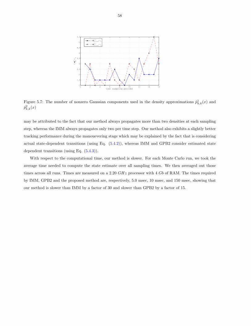
58
0 2 4 6 8 10 12 14 161
1.5
2
2.5
3
3.5
4
4.5
5
5.5
time (sampling periods)
||wk1||0
||ϖk,trun1,* ||
0
||ϖk,trun2,* ||
0
Figure 5.7: The number of nonzero Gaussian components used in the density approximations p1k,k(x) and
p2k,k(x)
may be attributed to the fact that our method always propagates more than two densities at each sampling
step, whereas the IMM always propagates only two per time step. Our method also exhibits a slightly better
tracking performance during the manouevering stage which may be explained by the fact that is considering
actual state-dependent transitions (using Eq. (5.4.2)), whereas IMM and GPB2 consider estimated state
dependent transitions (using Eq. (5.4.3)).
With respect to the computational time, our method is slower. For each Monte Carlo run, we took the
average time needed to compute the state estimate over all sampling times. We then averaged out those
times across all runs. Times are measured on a 2.20 GHz processor with 4 Gb of RAM. The times required
by IMM, GPB2 and the proposed method are, respectively, 5.0 msec, 10 msec, and 150 msec, showing that
our method is slower than IMM by a factor of 30 and slower than GPB2 by a factor of 15.

59
Chapter 6
Bilateral Counterparty Risk Valuation
6.1 Introduction
It has been reported by Canabarro and Duffie (2004) that the volume of outstanding over-the-counter
derivatives has grown exponentially over the past 15 years. More specifically, market surveys conducted by
the International Swaps and Derivatives Association (ISDA) show notional amounts of outstanding interest
rate and currency swaps reaching 866 billion US dollars in 1987, 17.7 trillion US dollars in 1995, and 99.8
trillion US dollars in 2002; an astonishing compounded growth rate of 37.2% per year. Over-the-counter
contracts are traded (and privately negotiated) directly between the two parties, without going through an
exchange or other intermediary. Such contracts include, for example, credit default swaps, forward rate
agreements, and interest rate swaps see (see Brigo and Mercurio, 2006). Since they are not traded on an
exchange, there is no central clearinghouse that insures against the default risk of both parties, therefore
both parties of the contracts are exposed to counterparty risk, namely the risk that one party defaults on its
payment obligation.
Correct modeling and valuation of counterparty risk has become even more relevant in recent years as
some protection sellers such as mono-line insurers or investment banks have witnessed increasing default
probabilities or even default events, the case of Lehman Brothers being a clear example. Moreover, regula-
tory issues related to the IAS 39 framework encourage the inclusion of counterparty risk into the contract
valuation.
In this chapter we introduce a general arbitrage-free valuation framework for bilateral counterparty
default risk and assume absence of guarantees such as collateral. We call the two parties of the contract
the investor and her counterparty. By ‘bilateral’ we intend to point out that the default of the investor is
included into the framework, contrary to earlier works. This brings about symmetry, so that the price of
the position including counterparty risk to the investor is exactly the opposite of the price of the position to
the counterparty. This is clearly not the case if each of the two parties computes the present value assuming
itself to be default-free and allowing for default of the other party only. This asymmetry would not matter in
situations where financial investors had high credit quality and counterparties rather low one. Indeed, in such
a case both parties would consider the investor as default-free and the counterparty as defaultable, so that
inclusion of the investor default would be pointless, given that it happens in almost no scenario. However,

60
recent events show that it is no longer realistic to take the credit quality of the financial institution for
granted and to be highly superior to that of a general counterparty, no matter how prestigious or important
the financial institution.
This chapter generalizes to the bilateral symmetric case the asymmetric unilateral setting proposed
in Brigo and Chourdakis (2008), Brigo and El-Bachir (2008), Brigo and Masetti (2005), and Brigo and
Pallavicini (2007), where only the counterparty is subject to default risk, while the investor is assumed
to be default free. We provide a general formula that gives the bilateral risk credit valuation adjustment
(BR-CVA) for portfolios exchanged between a default risky investor and a default risky counterparty. Such
formula shows that the adjustment to the investor is the difference between two discounted options terms, a
discounted call option in scenarios of early default time of the counterparty minus a discounted put option
in scenarios of early default times of the investor, both options being on the residual net present value of the
portfolio at the relevant default times and having zero strike. The BR-CVA seen from the point of view of
the counterparty is exactly the opposite. We allow for correlation between default of the investor, default of
the counterparty and underlying portfolio risk factors, and for volatilities and dynamics in the credit spreads
and in the underlying portfolio, all arbitrage free.
We then specialize our analysis to Credit Default Swaps (CDS) as underlying portfolio, generalizing the
work of Brigo and Chourdakis (2008) who deal with unilateral and asymmetric counterparty risk for these
contracts. Featuring a CDS as underlying, a third default time enters the picture, namely the default time
for the reference credit of the CDS. We therefore assume that all three entities are subject to default risk
and that the default events of investor, counterparty and reference credit are correlated. We then propose a
numerical methodology to evaluate the resulting BR-CVA formula. We investigate the impact of both credit
spread volatility and default correlation on the credit valuation adjustment. Most of previous approaches on
CDS counterparty risk only focus on unilateral counterparty risk. One exception is Duffie and Huang (1996)
who considers the bilateral setting under a much simpler static model of counterparty exposure, which is
calculated on average across a market. Moreover, most of the existing studies ignore the effect of volatility
on the adjustment and mainly focus on default correlation. Hull and White (2000) study the counterparty
risk problem by resorting to barrier correlated models. Collin-Dufresne et al. (2004) model default intensities
as deterministic constants using default indicators of other names as feeds. The need for explicitly modeling
credit spread volatility is even more pronounced in the case of CDS if the underlying reference contract is
itself a CDS, as the credit valuation adjustment would involve CDS options and it is very undesirable to
model options without volatility in the underlying asset.
We analyze the impact of credit spreads volatility and default correlation through some numerical ex-
amples and find significant sensitivity to credit spreads volatility, especially under scenarios of large default
correlation.
The rest of the chapter is organized as follows. Section 6.2 gives the general BR-CVA formula and
refers to the appendix for the mathematical proof. Section 6.3 defines the underlying framework needed for
applying the above methodology to credit default swaps, including the stochastic intensity model and the
trivariate copula function for correlating defaults. Section 6.4 develops a numerical method to implement

61
the formula in the case when the underlying contract is a CDS and gives the pseudo code of the algorithm
used to run numerical simulations. Section 6.5 present numerical experiments on different default correlation
scenarios and changes in credit spread volatility. Section 6.6 presents a specific application for computing
the mark-to-market value of a CDS contract agreed between British Airways, Lehman Brothers, and Royal
Shell.
6.2 Arbitrage-Free Valuation of Bilateral Counterparty Risk
We refer to the two names involved in the financial contract and subject to default risk as
investor → name “0”
counterparty → name “2”
In cases where the portfolio exchanged by the two parties is also a default sensitive instrument, we
introduce a third name referring to the reference credit of that portfolio
reference credit → name “1”
If the portfolio is not default sensitive then name “1” can be removed.
We denote by τ0, (τ1), and τ2, respectively the default times of the investor, (reference credit), and
counterparty. We place ourselves in a probability space (Ω,G,Gt,Q). The filtration Gt models the flow of
information of the whole market, including credit and Q is the risk neutral measure. This space is endowed
also with a right-continuous and complete sub-filtration Ft representing all the observable market quantities
but the default event, thus Ft ⊆ Gt := Ft ∨Ht. Here, Ht = σ(τ0 ≤ u(∨τ1 ≤ u) ∨ τ2 ≤ u : u ≤ t) is
the right-continuous filtration generated by the default events, either of the investor or of his counterparty
(and of the reference credit if the underlying portfolio is credit sensitive).
Let us call T the final maturity of the payoff which we need to evaluate and let us define the stopping
time
τ = minτ0, τ2 (6.2.1)
If τ > T , there is neither default of the investor, nor of his counterparty during the life of the contract and
they both can fulfill the agreements of the contract. On the contrary, if τ ≤ T then either the investor or her
counterparty (or both) defaults. At τ , the Net Present Value (NPV) of the residual payoff until maturity is
computed. We then distinguish two cases:
• τ = τ2. If the NPV is negative (respectively positive) for the investor (defaulted counterparty), it
is completely paid (received) by the investor (defaulted counterparty) itself. If the NPV is positive
(negative) for the investor (counterparty), only a recovery fraction REC,2 of the NPV is exchanged.
• τ = τ0. If the NPV is positive (respectively negative) for the defaulted investor (counterparty), it
is completely received (paid) by the defaulted investor (counterparty) itself. If the NPV is negative
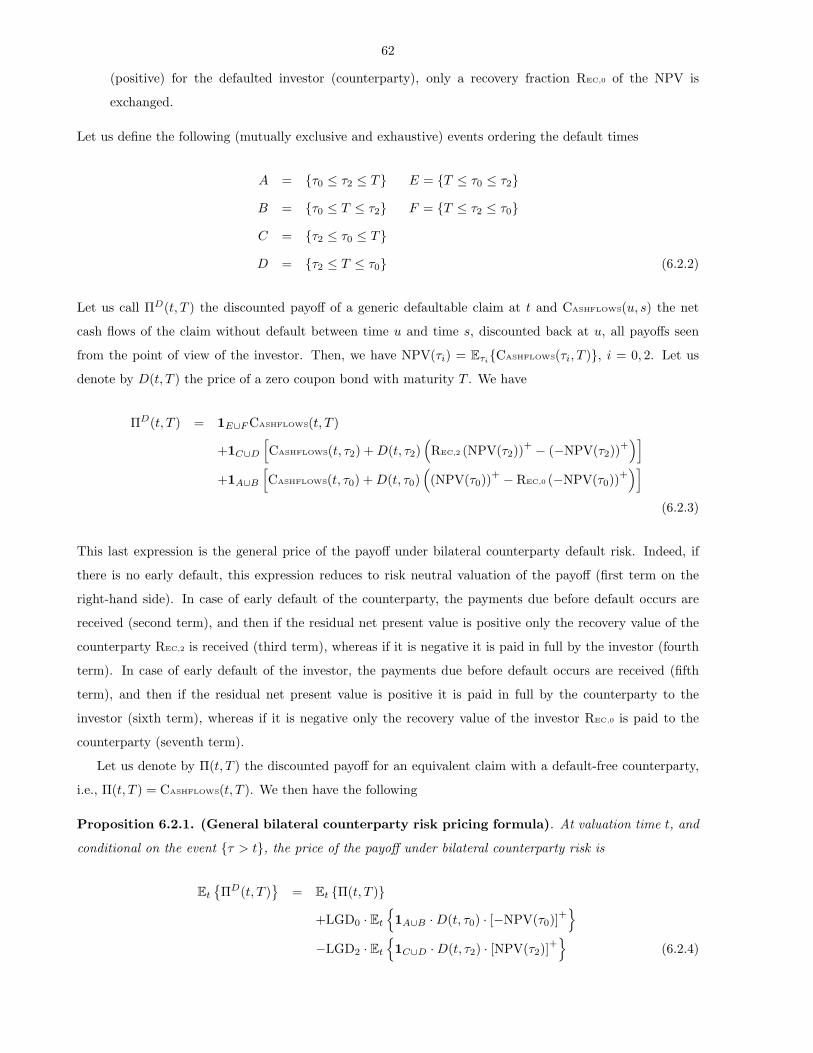
62
(positive) for the defaulted investor (counterparty), only a recovery fraction REC,0 of the NPV is
exchanged.
Let us define the following (mutually exclusive and exhaustive) events ordering the default times
A = τ0 ≤ τ2 ≤ T E = T ≤ τ0 ≤ τ2
B = τ0 ≤ T ≤ τ2 F = T ≤ τ2 ≤ τ0
C = τ2 ≤ τ0 ≤ T
D = τ2 ≤ T ≤ τ0 (6.2.2)
Let us call ΠD(t, T ) the discounted payoff of a generic defaultable claim at t and CASHFLOWS(u, s) the net
cash flows of the claim without default between time u and time s, discounted back at u, all payoffs seen
from the point of view of the investor. Then, we have NPV(τi) = EτiCASHFLOWS(τi, T ), i = 0, 2. Let us
denote by D(t, T ) the price of a zero coupon bond with maturity T . We have
ΠD(t, T ) = 1E∪FCASHFLOWS(t, T )
+1C∪D[CASHFLOWS(t, τ2) +D(t, τ2)
(REC,2 (NPV(τ2))
+ − (−NPV(τ2))+)]
+1A∪B[CASHFLOWS(t, τ0) +D(t, τ0)
((NPV(τ0))
+ − REC,0 (−NPV(τ0))+)]
(6.2.3)
This last expression is the general price of the payoff under bilateral counterparty default risk. Indeed, if
there is no early default, this expression reduces to risk neutral valuation of the payoff (first term on the
right-hand side). In case of early default of the counterparty, the payments due before default occurs are
received (second term), and then if the residual net present value is positive only the recovery value of the
counterparty REC,2 is received (third term), whereas if it is negative it is paid in full by the investor (fourth
term). In case of early default of the investor, the payments due before default occurs are received (fifth
term), and then if the residual net present value is positive it is paid in full by the counterparty to the
investor (sixth term), whereas if it is negative only the recovery value of the investor REC,0 is paid to the
counterparty (seventh term).
Let us denote by Π(t, T ) the discounted payoff for an equivalent claim with a default-free counterparty,
i.e., Π(t, T ) = CASHFLOWS(t, T ). We then have the following
Proposition 6.2.1. (General bilateral counterparty risk pricing formula). At valuation time t, and
conditional on the event τ > t, the price of the payoff under bilateral counterparty risk is
EtΠD(t, T )
= Et Π(t, T )
+LGD0 · Et1A∪B ·D(t, τ0) · [−NPV(τ0)]
+
−LGD2 · Et1C∪D ·D(t, τ2) · [NPV(τ2)]
+
(6.2.4)
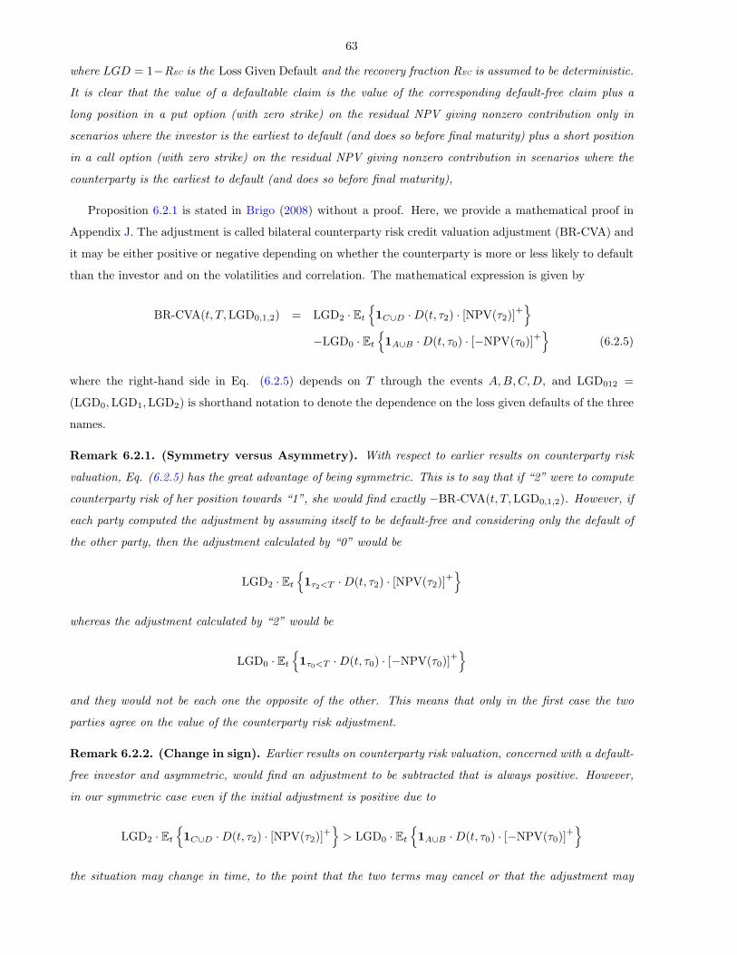
63
where LGD = 1−REC is the Loss Given Default and the recovery fraction REC is assumed to be deterministic.
It is clear that the value of a defaultable claim is the value of the corresponding default-free claim plus a
long position in a put option (with zero strike) on the residual NPV giving nonzero contribution only in
scenarios where the investor is the earliest to default (and does so before final maturity) plus a short position
in a call option (with zero strike) on the residual NPV giving nonzero contribution in scenarios where the
counterparty is the earliest to default (and does so before final maturity),
Proposition 6.2.1 is stated in Brigo (2008) without a proof. Here, we provide a mathematical proof in
Appendix J. The adjustment is called bilateral counterparty risk credit valuation adjustment (BR-CVA) and
it may be either positive or negative depending on whether the counterparty is more or less likely to default
than the investor and on the volatilities and correlation. The mathematical expression is given by
BR-CVA(t, T,LGD0,1,2) = LGD2 · Et1C∪D ·D(t, τ2) · [NPV(τ2)]
+
−LGD0 · Et1A∪B ·D(t, τ0) · [−NPV(τ0)]
+
(6.2.5)
where the right-hand side in Eq. (6.2.5) depends on T through the events A,B,C,D, and LGD012 =
(LGD0,LGD1,LGD2) is shorthand notation to denote the dependence on the loss given defaults of the three
names.
Remark 6.2.1. (Symmetry versus Asymmetry). With respect to earlier results on counterparty risk
valuation, Eq. (6.2.5) has the great advantage of being symmetric. This is to say that if “2” were to compute
counterparty risk of her position towards “1”, she would find exactly −BR-CVA(t, T,LGD0,1,2). However, if
each party computed the adjustment by assuming itself to be default-free and considering only the default of
the other party, then the adjustment calculated by “0” would be
LGD2 · Et1τ2<T ·D(t, τ2) · [NPV(τ2)]
+
whereas the adjustment calculated by “2” would be
LGD0 · Et1τ0<T ·D(t, τ0) · [−NPV(τ0)]
+
and they would not be each one the opposite of the other. This means that only in the first case the two
parties agree on the value of the counterparty risk adjustment.
Remark 6.2.2. (Change in sign). Earlier results on counterparty risk valuation, concerned with a default-
free investor and asymmetric, would find an adjustment to be subtracted that is always positive. However,
in our symmetric case even if the initial adjustment is positive due to
LGD2 · Et1C∪D ·D(t, τ2) · [NPV(τ2)]
+> LGD0 · Et
1A∪B ·D(t, τ0) · [−NPV(τ0)]
+
the situation may change in time, to the point that the two terms may cancel or that the adjustment may

64
change sign as the credit quality of “0” deteriorates and that of “2” improves, so that the inequality changes
direction.
6.3 Application to Credit Default Swaps
In this section we use the formula developed in Section 6.2 to evaluate the BR-CVA in credit default swap
contracts (CDS). Section 6.3.1 recalls the general formula for CDS evaluation. Section 6.3.2 introduces the
copula models used to correlate the default events. Section 6.3.3 recalls the CIR model used for the stochastic
intensity of the three names. Section 6.3.4 applies the general BR-CVA formula to calculate the adjustment
for CDS contracts.
6.3.1 CDS Payoff
We assume deterministic interest rates, which leads to independence between τ1 and D(0, t). Our results
hold also true for the case of stochastic rates independent of default times. The receiver CDS valuation,
for a CDS selling protection LGD1 at time 0 for default of the reference entity between times Ta and Tb in
exchange of a periodic premium rate S1 is given by
CDSa,b(0, S1,LGD1) = S1
[−∫ Tb
Ta
D(0, t)(t− Tγ(t)−1)dQ(τ1 > t)
+b∑
i=a+1
αiD(0, Ti)Q(τ1 > Ti)]
+LGD1
[∫ Tb
Ta
D(0, t)dQ(τ1 > t)
](6.3.1)
where γ(t) is the first payment period Tj following time t. Let us denote by
NPV(Tj , Tb) := CDSa,b(Tj , S,LGD1) (6.3.2)
the residual NPV of a receiver CDS between Ta and Tb evaluated at time Tj , with Ta < Tj < Tb. Eq.
(6.3.2) can be written similarly to Eq. (6.3.1), except that now evaluation occurs at time Tj and has to be
conditioned on the information set available to the market at Tj . This leads to
CDSa,b(Tj , S1,LGD1) = 1τ1>Tj CDSa,b(Tj , S1, LGD1)
:= 1τ1>Tj
S1
[−∫ Tb
maxTa,TjD(Tj , t)(t− Tγ(t)−1)dQ(τ1 > t|GTj )
+b∑
i=maxa,j+1
αiD(Tj , Ti)Q(τ1 > Ti|GTj)]
+LGD1
[ ∫ Tb
maxTa,TjD(Tj , t)dQ(τ1 > t|GTj )
](6.3.3)
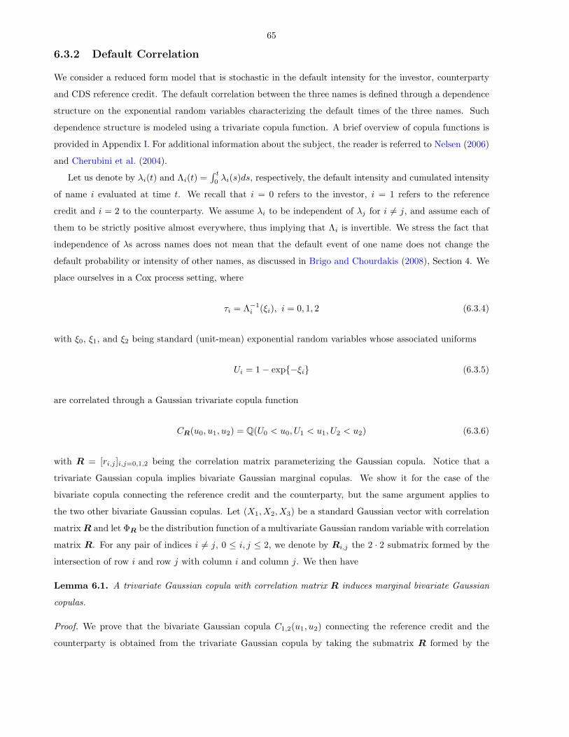
65
6.3.2 Default Correlation
We consider a reduced form model that is stochastic in the default intensity for the investor, counterparty
and CDS reference credit. The default correlation between the three names is defined through a dependence
structure on the exponential random variables characterizing the default times of the three names. Such
dependence structure is modeled using a trivariate copula function. A brief overview of copula functions is
provided in Appendix I. For additional information about the subject, the reader is referred to Nelsen (2006)
and Cherubini et al. (2004).
Let us denote by λi(t) and Λi(t) =∫ t0λi(s)ds, respectively, the default intensity and cumulated intensity
of name i evaluated at time t. We recall that i = 0 refers to the investor, i = 1 refers to the reference
credit and i = 2 to the counterparty. We assume λi to be independent of λj for i 6= j, and assume each of
them to be strictly positive almost everywhere, thus implying that Λi is invertible. We stress the fact that
independence of λs across names does not mean that the default event of one name does not change the
default probability or intensity of other names, as discussed in Brigo and Chourdakis (2008), Section 4. We
place ourselves in a Cox process setting, where
τi = Λ−1i (ξi), i = 0, 1, 2 (6.3.4)
with ξ0, ξ1, and ξ2 being standard (unit-mean) exponential random variables whose associated uniforms
Ui = 1− exp−ξi (6.3.5)
are correlated through a Gaussian trivariate copula function
CR(u0, u1, u2) = Q(U0 < u0, U1 < u1, U2 < u2) (6.3.6)
with R = [ri,j ]i,j=0,1,2 being the correlation matrix parameterizing the Gaussian copula. Notice that a
trivariate Gaussian copula implies bivariate Gaussian marginal copulas. We show it for the case of the
bivariate copula connecting the reference credit and the counterparty, but the same argument applies to
the two other bivariate Gaussian copulas. Let (X1, X2, X3) be a standard Gaussian vector with correlation
matrix R and let ΦR be the distribution function of a multivariate Gaussian random variable with correlation
matrix R. For any pair of indices i 6= j, 0 ≤ i, j ≤ 2, we denote by Ri,j the 2 · 2 submatrix formed by the
intersection of row i and row j with column i and column j. We then have
Lemma 6.1. A trivariate Gaussian copula with correlation matrix R induces marginal bivariate Gaussian
copulas.
Proof. We prove that the bivariate Gaussian copula C1,2(u1, u2) connecting the reference credit and the
counterparty is obtained from the trivariate Gaussian copula by taking the submatrix R formed by the
66
intersection of rows 1 and 2 with columns 1 and 2. We have
Q(U1 < u1, U2 < u2) = Q(U1 < u1, U2 < u2, U3 < 1)
= CR(u1, u2, 1)
= limb→1−
ΦR(Φ−1(u1),Φ−1(u2),Φ−1(b))
= limb→1−
Q(X1 < Φ−1(u1), X2 < Φ−1(u2), X3 < Φ−1(b))
= Q(X1 < Φ−1(u1), X2 < Φ−1(u2)) ·
limb→1−
Q(X3 < Φ−1(b)|X1 < Φ−1(u1), X2 < Φ−1(u2))
= ΦR1,2(Φ−1(u1),Φ−1(u2))
:= C1,2(u1, u2) (6.3.7)
By a similar calculation, the bivariate copula connecting the investor and the reference credit is given by C0,1
with associated correlation matrix R0,1 and the bivariate copula connecting the investor and the counterparty
is given by C0,2 with associated correlation matrix R0,2.
6.3.3 CIR Stochastic Intensity Model
We use the CIR process (see Cox et al., 1985) to model the default intensity of the investor, reference credit
and counterparty. We do not introduce correlation between the three intensity processes, but model default
correlation through a trivariate copula function on the exponential triggers of the default times. This is
because typically spread correlation has a much lower impact on dependence of default times than default
correlation. The correlation structure underlying the trivariate copula function may be estimated by the
implied correlation in the quoted indices tranches markets such as i-Traxx and CDX or calculated from the
asset correlation of the names. We assume the following stochastic intensity model Brigo and Alfonsi (2005),
Brigo and El-Bachir (2008) for the three names
λj(t) = yj(t) + ψj(t;βj), t ≥ 0, j = 0, 1, 2 (6.3.8)
where ψ is a deterministic function, depending on the parameter vector β (which includes y0), that is
integrable on closed intervals. We assume each yj to be a Cox Ingersoll Ross (CIR) process (see Brigo and
Mercurio, 2006) given by
dyj(t) = κj(µj − yj(t))dt+ νj
√yj(t)dZj(t) + JMt,jdMj(t), j = 0, 1, 2 (6.3.9)
where Js are i.i.d. positive jump sizes that are exponentially distributed with mean χj , and Mj are Poisson
processes with intensity mj measuring the arrival of jumps in the intensity λj . The parameter vectors are
βj = (κj , µj , νj , yj(0), χj ,mj) with each vector component being a positive deterministic constant. We relax
the condition of inaccessibility of the origin 2κjµj > ν2j so that we do not limit the CDS implied volatility
generated by the model. We assume the Zj to be standard Brownian motion processes under the risk-neutral

67
measure. We define the following integrated quantities which will be extensively used in the remainder of
the paper
Λj(t) =∫ t
0
λj(s)ds, Yj(t) =∫ t
0
yj(s)ds, Ψj(t;βj) =∫ t
0
ψj(s;βj)ds (6.3.10)
Here, we focus on intensities without jumps, i.e., mj = 0. Brigo and El-Bachir (2008) consider in detail the
tractable model with jumps, and this extension will be applied in future work.
6.3.4 Bilateral Risk Credit Valuation Adjustment for Receiver CDS
We next proceed to the valuation of the BR-CVA adjustment for the case of CDS payoff given by Eq. (6.3.1).
We state the result as a proposition.
Proposition 6.3.1. The BR-CVA at time t for a receiver CDS contract (protection seller) running from
time Ta to time Tb with premium S is given by
BR-CVA-CDSa,b(t, S,LGD0,1,2) = LGD2 · Et1C∪D ·D(t, τ2) ·
[1τ1>τ2CDSa,b(τ2, S, LGD1)
]+−LGD0 · Et
1A∪B ·D(t, τ0) ·
[−1τ1>τ0CDSa,b(τ0, S, LGD1)
]+(6.3.11)
Proof. We have
Et1C∪D ·D(t, τ2) · [NPV(τ2)]
+
= Et1C∪D ·D(t, τ2) · [CDSa,b(τ2, S,LGD1)]
+
= Et1C∪D ·D(t, τ2) ·
[1τ1>τ2CDSa,b(τ2, S,LGD1)
]+(6.3.12)
where the first equality in Eq. (6.3.12) follows by definition, while the last equality follows from Eq. (6.3.3).
Similarly, we have
Et1A∪B ·D(t, τ0) · [−NPV(τ0)]
+
= Et1A∪B ·D(t, τ0) · [−CDSa,b(τ0, S,LGD1)]
+
= Et1A∪B ·D(t, τ0) ·
[−1τ1>τ0CDSa,b(τ0, S,LGD1)
]+(6.3.13)
The proof follows using the expression of BR-CVA which is given by Eq. (6.2.5).
To summarize, in order to compute the counterparty risk adjustment, we determine the value of the CDS
contract on the reference credit “1”, at the point in time τ2 at which the counterparty “2” defaults. The
reference name “1” has survived this point and there is a bivariate copula C1,2 given by Eq. (6.3.7) which
connects the default times of the reference credit and the counterparty “2”. Similarly, in order to compute
the investor risk adjustment, we determine the value of the CDS contract on the reference credit “1” at the

68
point in time τ0 at which the counterparty “0” defaults. The reference name “1” has survived this point and
there is a bivariate copula C0,1 given by the analogous of Eq. (6.3.7) which connects the default times of
the reference credit and the investor “0”. It is clear from Eq. (6.3.3) that the only terms we need to know
in order to compute (6.3.12) and (6.3.13) are
1τ1>τ2Q(τ1 > t|Gτ2) (6.3.14)
and
1τ1>τ0Q(τ1 > t|Gτ0) (6.3.15)
In the next section, we generalize the numerical method proposed in Brigo and Chourdakis (2008) to
calculate quantities (6.3.14) and (6.3.15) for the bilateral counterparty case.
6.4 Monte-Carlo Evaluation of the BR-CVA Adjustment
We propose a numerical method based on Monte-Carlo simulations to calculate the BR-CVA for the case of
CDS contracts. Section 6.4.1 specifies the simulation method used to generate the sample paths of the CIR
process. Section 6.4.2 gives a method to calculate (6.3.14), while Section 6.4.3 gives the complete numerical
algorithm for calculating the BR-CVA in (6.2.4).
6.4.1 Simulation of CIR Process
We use the well-known fact (see Brigo and Mercurio, 2006) that the distribution of y(t) given y(u), for some
u < t is, up to a scale factor, a noncentral chi-square distribution. More precisely, the transition law of y(t)
given y(u) can be expressed as
y(t) =ν2(1− e−κ(t−u))
4κχ′d
(4κe−κ(t−u)
ν2(1− e−κ(t−u))y(u)
)(6.4.1)
where
d =4κµν2
(6.4.2)
and χ′u(v) denotes a noncentral chi-square random variable with u degrees of freedom and non-centrality
parameter v. In this way, if we know y(0), we can simulate the process y(t) exactly on a discrete time grid
by sampling from the noncentral chi-square distribution.
6.4.2 Calculation of Survival Probability
We state the result in the form of a proposition. Such result will be used in Section 6.4.3 to develop a
numerical algorithm for computing the BR-CVA.
69
Proposition 6.4.1.
1τ1>τ2Q(τ1 > t|Gτ2) = 1A + 1t<τ21τ1>τ2
∫ 1
U1
FΛ1(t)(− log(1− u1))dC1|2(u1;U2)
where
A = t < τ2 < τ1
C1|2 =f(u, v)− f(U1, v)
1− f(U1, v)
U1 := 1− exp−Y1(τ2)−Ψ1(τ2;β1)
f(u, v) = Φ
Φ−1(u)− r1,2Φ−1(v)√1− r21,2
(6.4.3)
and FΛ1(t) denotes the cumulative distribution function of the cumulative (shifted) intensity of the CIR
process which can be retrieved inverting the characteristic function of the integrated CIR process. The proof
of the proposition is reported in Appendix K.
6.4.3 The Numerical BR-CVA Adjustment Algorithm
We give the pseudo code of the numerical algorithm used to calculate the BR-CVA for the CDS payer and
receiver. In the pseudo code below, the variable αi represents the time elapsing between payment period ti−1
and ti measured in years, the variable ∆ represents the fineness of the grid used to evaluate the integral of the
survival probability in Eq. (6.4.3) and the variable δ represents the fineness of the time grid used to evaluate
the integral in Eq. (6.3.3). The variable xmax represents the maximum x value for which the cumulative
distribution function is implied from the characteristic function. The expression CDF(xk) corresponds to a
subroutine call which calculates the cumulative distribution function at xk. This can be done by inversion
of the characteristic function of the integrated CIR process using fractional Fourier transform methods such
as in Chourdakis (2005). The inputs to the main procedure Calculate Adjustment are the number N
of Monte Carlo runs and the market quote S1 of the 5 year CDS spread of the reference entity.
6.5 Numerical Results
We consider an investor (name “0”) trading a five-years CDS contract on a reference name (name “1”)
with a counterparty (name “2”). Both the investor and the counterparty are subject to default risk. We
experiment on different levels of credit risk and credit risk volatility of the three names, which are specified
by the parameters of the CIR processes in Table 6.1. We recall that the survival probabilities associated
with a CIR intensity process are given by
Q(τi > t) := E[e−Yi(t)]
= PCIR(0, t,βi) (6.5.1)

70
Algorithm 1 [BR-CVA R,BR-CVA P] = Calculate Adjustment (N, S)for i = 1 : N do
Generate τ0, τ1, and τ2 using Eq. (6.3.5) and Eq. (6.3.6).if τ2 < τ0 and τ2 < Tb then
if τ1 > τ2 then[BR-CVA R 2, BR-CVA P 2] = CDSAdjust(Tγ(τ2), S, LGD1, 2)CUM BR-CVA R = CUM BR-CVA R + LGD2· BR-CVA R 2CUM BR-CVA P = CUM BR-CVA P + LGD2· BR-CVA P 2
end ifend ifif τ0 < τ2 and τ0 < Tb then
if τ1 > τ0 then[BR-CVA R 0, BR-CVA P 0] = CDSAdjust(Tγ(τ0), S, LGD1, 0)CUM BR-CVA R = CUM BR-CVA R - LGD0· BR-CVA R 0CUM BR-CVA P = CUM BR-CVA P - LGD0· BR-CVA P 0
end ifend if
end forBR-CVA R = CUM BR-CVA R / NBR-CVA P = CUM BR-CVA P / N
Algorithm 2 [CDSR, CDSP ] = CDSAdjust(Tj , S, LGD1, index)Term1 = Term2 = Term3 = 0tstart = max(Ta, Tj)Qprev = ComputeProb(tstart, Tj , index)for t = tstart + δ : δ : Tb doQcurr = ComputeProb(t, Tj , index)Term1 = Term1 +D(Tj , t− δ)(t− δ − Tγ(t−δ)−1)(Qcurr −Qprev)Term3 = Term3 +D(Tj , t− δ)(Qcurr −Qprev)Qprev = Qcurr
end forfor ti = tstart + αi : αi : Tb doQcurr = ComputeProb(ti, Tj , index)Term2 = Term2 + αi ·D(Tj , ti) ·Qcurr
end forCDSval = S · (Term2 − Term1) + LGD1 · Term3
if index == 2 thenCDSR = D(t, Tj) ·max(CDSval, 0)CDSP = D(t, Tj) ·max(−CDSval, 0)
end ifif index == 0 thenCDSR = D(t, Tj) ·max(−CDSval, 0)CDSP = D(t, Tj) ·max(CDSval, 0)
end if
Credit Risk Levels y(0) κ µ Credit Risk volatilities ν
low 0.0001 0.9 0.001 low 0.01middle 0.01 0.80 0.02 middle 0.2high 0.03 0.50 0.05 high 0.5
Table 6.1: The credit risk levels and credit risk volatilities parameterizing the CIR processes
where PCIR(0, t,βi) is the price at time 0 of a zero coupon bond maturing at time t under a stochastic interest
rate dynamics given by the CIR process with βi = (yi(0), κi, µi, νi) being the vector of CIR parameters,

71
Algorithm 3 Qi = ComputeProb(t, Tj , index)Uindex = 1− exp−Yindex(Tj)−Ψindex(Tj ;βindex)U1 = 1− exp−Y1(Tj)−Ψ1(Tj ;β1)for xk = 0 : ∆ : xmax dopk = CDF(xk)uk = 1− exp−xk − ψ1(t)Compute fk = C1|2(uk;Uindex) using Eq. (K.0.5) and Eq. (K.0.6)
end forQi =
∑(uk,pk,fk):uk>U1
pk(fk+1 − fk)
Maturity Low Risk Middle Risk High risk1y 0 92 2342y 0 104 2443y 0 112 2484y 1 117 2505y 1 120 2516y 1 122 2527y 1 124 2538y 1 125 2539y 1 126 25410y 1 127 254
Table 6.2: Break-even spreads in basis points generated using the parameters of the CIR processes in Table6.1. The first column is generated using low credit risk and credit risk volatility. The second column isgenerated using middle credit risk and credit risk volatility. The third column is generated using high creditrisk and credit risk volatility.
i = 0, 1, 2. Such price may be computed in close form (see Brigo and Mercurio, 2006) and is given by
PCIR(0, t,βi) = A(t, T )e−B(t,T )r(t) (6.5.2)
where
A(t, T ) =
[2hie(hi+κi)(T−t)/2
2hi + (κi + hi)(ehi(T−t)/2 − 1
)]2κiµi
B(t, T ) =2(ehi(T−t) − 1
)2hi + (κi + hi)
(ehi(T−t)/2 − 1
)hi =
√κ2i + 2ν2
i (6.5.3)
and rt denotes the risk-free interest rate at time t. We report in Table 6.2 the break-even spreads zeroing
(6.3.3) in S, with survival probabilities given by Eq. (6.5.1) and CIR parameters βlow, βmiddle, βhigh
obtained from Table 6.1.
The evaluation time t and the starting time Ta of the CDS contract are both set to zero. The end
time Tb of the contract is set to five years. It is assumed that payments are exchanged every three months.
The loss given defaults of the low, middle, and high risk entity are, respectively, set to LGDlow = 0.6,
LGDmiddle = 0.65, LGDhigh = 0.7. We assume that the spreads in Table 6.2 are the spreads quoted in

72
the markets for the three names under consideration. We recover the integrated shift Ψ(t;β) which makes
the model survival probabilities consistent with the market survival probabilities coming from Table 6.2
whenever we change the CIR parameters. In mathematical terms, for any i = 0, 1, 2, we impose that
Q(τi > t)model := E[e−Λi(t)]
= Q(τi > t)market (6.5.4)
The market survival probability for name “i” is bootstrapped from the market CDS quotes reported in
Table 6.2. Such bootstrap procedure is performed assuming a piecewise linear hazard rate function. From
the definition of the integrated process Ψj(t;βj) given in Eq. (6.3.10), we can restate Eq. (6.5.4) as
Ψi(t;βi) = log(
E[e−Yi(t)]Q(τi > t)market
)= log
(PCIR(0, t,βi)
Q(τi > t)market
)(6.5.5)
where the last equality in Eq. (6.5.5) follows from Eq. (6.5.1). We first study a case where the quoted
market spreads of the investor has a low credit risk profile (βlow), the reference entity has high credit risk
profile (βhigh), while the counterparty has middle credit risk (βmiddle). We vary the correlation between
reference credit and counterparty as well as the credit risk volatility ν1 of the reference credit. Since the
focus is mostly on credit spreads volatility, we calculate the implied CDS volatility produced by the choice
of parameters β1 = (y0(1), µ1, κ1, ν1) for a hypothetical CDS option, maturing in one year and in case of
exercise entering into a four year CDS contract on the underlying reference credit “1”. The objective of the
experiments is to measure the impact of correlation and credit spreads volatility on the BR-CVA. The triple
(x, y, z) represents the correlation of the trivariate Gaussian copula, with x denoting the correlation between
the investor and reference credit, y denoting the correlation between the investor and the counterparty and
z denoting the correlation between the reference credit and the counterparty. The values BR-CVA P and
BR-CVA R are respectively the Monte Carlo estimates of the CDS payer and receiver counterparty risk
adjustments. The theoretical formula for payer risk adjustment is given by
LGD2 · Et
1C∪D ·D(t, τ2) · [−NPV(τ2)]
+
−LGD0 · Et
1A∪B ·D(t, τ0) · [NPV(τ0)]
+
(6.5.6)
which follows from adapting the formula in Eq. (6.2.4), given for the receiver counterparty adjustment, to
the case of the payer counterparty adjustment. Tables 6.3 and 6.4 report the results obtained.
The scenarios considered in Table 6.3 and 6.4 assume an investor with an extremely low credit risk profile
and thus are similar to those considered in Brigo and Chourdakis (2008), where the investor is assumed to
be default-free. Therefore, it is not surprising that we find similar results. Similarly to them, we can see
that as the correlation between counterparty and reference credit increases, the BR-CVA decreases, except
for large correlation values where the BR-CVA goes down. This is the case because if the reference credit

73
(r01, r02, r12) Vol. parameter ν1 0.01 0.10 0.20 0.30 0.40 0.50CDS Implied vol 1.5% 15% 28% 37% 42% 42%
(0, 0, -0.99) BR-CVA P 0.0(0.0) 0.0(0.0) -0.0(0.0) -0.0(0.0) -0.0(0.0) -0.0(0.0)
BR-CVA R 28.6(1.3) 28.8(1.3) 28.7(1.3) 28.8(1.3) 28.7(1.3) 28.7(1.3)
(0, 0, -0.90) BR-CVA P 0.0(0.0) 0.0(0.0) -0.0(0.0) -0.0(0.0) 0.0(0.0) 0.1(0.1)
BR-CVA R 28.7(1.3) 28.8(1.3) 28.7(1.3) 28.8(1.3) 28.8(1.3) 28.6(1.3)
(0, 0, -0.60) BR-CVA P 0.0(0.0) 0.0(0.0) 0.0(0.0) 0.2(0.1) 0.2(0.1) 0.7(0.3)
BR-CVA R 26.5(1.3) 26.5(1.3) 26.0(1.3) 25.3(1.2) 24.8(1.2) 24.6(1.2)
(0, 0, -0.20) BR-CVA P 0.0(0.0) 0.4(0.1) 1.2(0.2) 2.4(0.4) 2.5(0.4) 2.2(0.4)
BR-CVA R 9.5(0.6) 9.8(0.6) 10.8(0.6) 11.4(0.7) 12.0(0.7) 12.2(0.7)
(0, 0, 0) BR-CVA P 5.7(0.3) 6.0(0.4) 6.2(0.5) 7.3(0.7) 7.1(0.8) 5.1(0.6)
BR-CVA R -0.0(0.0) 0.4(0.1) 1.8(0.2) 3.3(0.2) 4.3(0.3) 5.0(0.3)
(0, 0, 0.20) BR-CVA P 26.0(1.4) 25.5(1.4) 22.6(1.4) 19.8(1.4) 17.0(1.4) 14.5(1.3)
BR-CVA R -0.0(0.0) 0.0(0.0) 0.2(0.0) 0.4(0.0) 0.5(0.1) 0.6(0.1)
(0, 0, 0.60) BR-CVA P 76.3(4.6) 76.7(4.6) 66.6(4.1) 56.0(3.6) 48.9(3.2) 45.1(2.9)
BR-CVA R -0.0(0.0) -0.0(0.0) 0.0(0.0) 0.0(0.0) 0.0(0.0) 0.0(0.0)
(0, 0, 0.90) BR-CVA P 75.6(6.0) 76.5(6.0) 77.3(5.7) 65.9(5.0) 64.6(4.6) 62.6(4.4)
BR-CVA R -0.0(0.0) -0.0(0.0) 0.0(0.0) 0.0(0.0) 0.0(0.0) 0.0(0.0)
(0, 0, 0.99) BR-CVA P 0.0(0.0) 12.5(2.6) 40.6(4.3) 40.8(4.1) 54.9(4.5) 62.0(4.7)
BR-CVA R -0.0(0.0) -0.0(0.0) 0.0(0.0) 0.1(0.0) 0.1(0.0) 0.0(0.0)
Table 6.3: BR-CVA in basis points for the case when ν2 = 0.01 and ν0 = 0.01; numbers within roundbrackets represent the Monte-Carlo standard error. The CDS contract on the reference credit has a five-years maturity.
(r01, r02, r12) Vol. parameter ν1 0.01 0.10 0.20 0.30 0.40 0.50CDS Implied vol 1.5% 15% 28% 37% 42% 42%
(0, 0, -0.99) BR-CVA P 0.0(0.0) 0.0(0.0) -0.0(0.0) -0.0(0.0) -0.0(0.0) 0.1(0.1)
BR-CVA R 29.0(1.3) 28.7(1.3) 28.1(1.3) 28.8(1.3) 28.3(1.3) 29.1(1.3)
(0, 0, -0.90) BR-CVA P 0.0(0.0) 0.0(0.0) -0.0(0.0) -0.0(0.0) 0.1(0.1) 0.0(0.0)
BR-CVA R 29.8(1.4) 28.0(1.3) 27.7(1.3) 28.7(1.3) 27.6(1.3) 28.4(1.3)
(0, 0, -0.60) BR-CVA P 0.0(0.0) 0.0(0.0) 0.0(0.0) 0.3(0.1) 0.4(0.2) 0.5(0.2)
BR-CVA R 27.1(1.3) 24.8(1.2) 25.8(1.2) 24.6(1.2) 23.7(1.2) 24.1(1.2)
(0, 0, -0.20) BR-CVA P 0.0(0.0) 0.5(0.1) 1.7(0.3) 2.0(0.3) 3.1(0.5) 2.7(0.4)
BR-CVA R 9.3(0.6) 9.5(0.6) 10.9(0.6) 11.1(0.6) 11.3(0.7) 12.0(0.7)
(0, 0, 0) BR-CVA P 6.3(0.3) 5.3(0.4) 6.7(0.6) 6.7(0.7) 6.6(0.8) 6.0(0.7)
BR-CVA R -0.0(0.0) 0.3(0.0) 2.2(0.2) 3.4(0.2) 4.1(0.3) 4.9(0.3)
(0, 0, 0.20) BR-CVA P 25.8(1.4) 23.5(1.4) 21.3(1.3) 19.2(1.4) 16.8(1.4) 14.1(1.2)
BR-CVA R -0.0(0.0) -0.0(0.0) 0.3(0.0) 0.5(0.1) 0.7(0.1) 0.7(0.1)
(0, 0, 0.60) BR-CVA P 71.9(4.4) 70.2(4.4) 65.2(4.1) 55.1(3.6) 46.4(3.1) 42.4(2.9)
BR-CVA R -0.0(0.0) -0.0(0.0) 0.0(0.0) 0.0(0.0) 0.0(0.0) 0.0(0.0)
(0, 0, 0.90) BR-CVA P 77.3(5.9) 82.6(6.2) 77.9(5.8) 66.4(5.0) 63.6(4.5) 61.9(4.3)
BR-CVA R -0.0(0.0) -0.0(0.0) 0.0(0.0) 0.1(0.0) 0.0(0.0) 0.0(0.0)
(0, 0, 0.99) BR-CVA P 43.0(4.8) 49.8(5.1) 56.1(5.2) 50.2(4.5) 57.7(4.5) 62.3(4.7)
BR-CVA R 0.0(0.0) 0.1(0.0) 0.2(0.1) 0.3(0.1) 0.3(0.1) 0.3(0.1)
Table 6.4: BR-CVA in basis points for the case when ν2 = 0.2 and ν0 = 0.01; numbers within round bracketsrepresent the Monte-Carlo standard error. The CDS contract on the reference credit has a five-years maturity.

74
(r01, r02, r12) Base Scenario Risky Counterparty Risky Investor Risky Ref Safe Ref
(0, 0, 0) 6.2(0.4) 3.6(0.2) -0.8(0.1) -0.0(0.0) 5.5(0.4)
(0, 0, 0.1) 15.1(0.9) 11.9(0.5) -0.7(0.1) 0.0(0.0) 13.8(0.8)
(0, 0, 0.3) 36.6(2.1) 35.1(1.4) -0.5(0.2) 0.2(0.0) 35.0(2.0)
(0, 0, 0.6) 72.7(4.4) 88.2(3.8) -0.8(0.0) 0.7(0.1) 69.7(4.4)
(0, 0, 0.9) 75.2(5.9) 194.2(8.2) -0.8(0.0) 1.4(0.4) 71.0(5.8)
(0, 0, 0.99) 25.3(3.7) 281.2(11.5) -0.8(0.0) 1.9(0.7) 19.6(3.3)
(0, 0.1, 0) 5.9(0.4) 3.5(0.2) -0.8(0.1) -0.0(0.0) 5.0(0.4)
(0, 0.3, 0) 6.2(0.4) 3.5(0.2) -0.8(0.0) -0.0(0.0) 5.1(0.4)
(0, 0.6, 0) 5.9(0.4) 3.2(0.2) -0.8(0.0) -0.0(0.0) 4.4(0.3)
(0, 0.9, 0) 5.2(0.3) 3.4(0.2) -0.8(0.0) -0.0(0.0) 4.0(0.3)
(0, 0.99, 0) 5.1(0.3) 3.2(0.2) -0.8(0.0) -0.0(0.0) 3.5(0.3)
(0.1, 0, 0) 6.1(0.4) 3.6(0.2) -0.1(0.0) 0.0(0.0) 5.8(0.4)
(0.3, 0, 0) 6.2(0.4) 3.6(0.2) -0.0(0.0) 0.0(0.0) 5.8(0.4)
(0.6, 0, 0) 6.0(0.4) 3.6(0.2) 0.0(0.0) 0.0(0.0) 5.8(0.4)
(0.9, 0, 0) 6.0(0.4) 3.6(0.2) -0.0(0.0) -0.1(0.0) 6.0(0.4)
(0.99, 0, 0) 6.2(0.4) 3.6(0.2) -1.7(0.1) -0.1(0.0) 6.1(0.4)
Table 6.5: BR-CVA under five different riskiness scenarios. The CIR volatilities are set to ν0 = ν1 = ν2 = 0.1.The correlation triple has only one nonzero entry
and the counterparty are 99% correlated, then the exponential triggers ξ1 and ξ2 are almost identical; if we
consider the scenario where ν1 = ν2 = 0.01, then the intensity of both processes are almost deterministic,
with λ1 > λ2 having the name “1” high credit risk and name “2” middle credit risk. Thus, to a first
approximation τ1 = ξ1λ1
is higher than τ2 = ξ2λ2
, and consequently the reference credit always defaults before
the counterparty, resulting in no adjustment. Table 6.4 has qualitatively a similar behavior although the
larger value of the counterparty volatility ν2 = 0.2 tends to smooth out the negligible BR-CVA obtained
in Table 6.3 for small values of reference credit volatility and high default correlation between counterparty
and reference credit.
Tables 6.5, 6.6 and 6.7 report the BR-CVA adjustments for the Payer CDS under a set of five different
riskiness scenarios. The assignments of credit risks in Table 6.1 to the three names determine the scenario
in place. We have:
• Scenario 1 (Base Scenario). The investor has low credit risk, the reference entity has high credit risk,
the counterparty has middle credit risk
• Scenario 2 (Risky Counterparty). The investor has low credit risk, the reference entity has middle
credit risk and the counterparty has high credit risk.
• Scenario 3 (Risky Investor). The counterparty has low credit risk, the reference entity has middle
credit risk, while the investor has high credit risk.
• Scenario 4 (Risky Reference entity). Both investor and counteparty have middle credit risk, while the
reference entity has high credit risk.
• Scenario 5 (Safe Reference entity). Both investor and counterparty have high credit risk, while the
reference entity has low credit risk.

75
(r01, r02, r12) Base Scenario Risky Counterparty Risky Investor Risky Ref Safe Ref
(0, 0.5, 0.5) 54.8(3.5) 62.7(2.8) -0.6(0.2) 0.5(0.0) 47.8(3.3)
(0, 0.2, 0.9) 72.9(5.8) 183.0(8.0) -0.8(0.0) 1.3(0.4) 64.5(5.6)
(0, 0.9, 0.2) 21.0(1.3) 20.3(0.8) -0.8(0.0) 0.1(0.0) 15.2(1.2)
(0.5, 0, 0.5) 64.3(3.7) 67.9(2.9) -0.0(0.0) 0.6(0.0) 61.7(3.7)
(0.2, 0, 0.9) 81.8(6.2) 193.4(8.2) -0.1(0.0) 1.5(0.4) 79.8(6.1)
(0.9, 0, 0.2) 27.0(1.5) 23.4(0.9) 0.0(0.1) 0.1(0.0) 26.3(1.4)
(0.5, 0.5, 0) 6.6(0.4) 3.4(0.2) -0.0(0.0) 0.0(0.0) 6.2(0.4)
(0.2, 0.9, 0) 5.5(0.3) 3.5(0.2) -0.1(0.0) 0.0(0.0) 4.3(0.3)
(0.9, 0.2, 0) 7.0(0.4) 3.5(0.2) -0.0(0.0) -0.0(0.0) 6.1(0.4)
Table 6.6: BR-CVA under five different riskiness scenarios. The CIR volatilities are set to ν0 = ν1 = ν2 = 0.1.The correlation triple has two nonzero entries
(r01, r02, r12) Base Scenario Risky Counterparty Risky Investor Risky Ref Safe Ref
(0.8, 0.5, 0.2) 25.9(1.4) 23.3(0.9) 0.2(0.1) 0.1(0.0) 25.1(1.4)
(0.8, 0.2, 0.5) 60.9(3.6) 65.9(2.9) 0.3(0.2) 0.5(0.0) 60.1(3.6)
(0.5, 0.8, 0.2) 24.1(1.4) 22.5(0.9) 0.0(0.1) 0.1(0.0) 19.9(1.3)
(0.5, 0.2, 0.8) 89.0(6.0) 142.3(6.2) -0.0(0.0) 1.1(0.2) 84.0(5.8)
(0.2, 0.5, 0.8) 75.1(5.5) 133.1(6.0) -0.1(0.0) 0.9(0.2) 62.2(5.1)
(0.2, 0.8, 0.5) 51.7(3.4) 59.3(2.7) -0.1(0.0) 0.4(0.0) 38.5(3.0)
(0.2, 0.2, 0.2) 25.2(1.4) 22.5(0.9) 0.1(0.1) 0.1(0.0) 22.8(1.3)
(0.5, 0.5, 0.5) 58.2(3.6) 64.4(2.8) 0.4(0.3) 0.5(0.0) 53.7(3.5)
(0.8, 0.8, 0.8) 79.5(5.7) 132.0(6.0) -0.0(0.0) 0.8(0.2) 69.8(5.3)
Table 6.7: BR-CVA under five different riskiness scenarios. The CIR volatilities are set to ν0 = ν1 = ν2 = 0.1.The correlation triple has all nonzero entries
Tables 6.5, 6.6, and 6.7 show the important role played by default correlation. For example, if one looks
at the second column of those tables, one notices that as the correlation between counterparty and reference
credit gets larger, the BR-CVA increases due to the copula contagion coming from the default of the reference
credit and to the large riskiness level of the counterparty. If the only correlation is between reference credit
and counterparty, then the adjustment is the largest, while when correlation starts manifesting also between
all other pairs (see second column of Tables 6.6 and 6.7), then the adjustment tends to decrease, since the
default contagion induced by investor tends to reduce the number of times when the risky counterparty is
the earliest to default.
An interesting pattern emerges from the first two columns and five rows of Table 6.5. Although the
counterparty is riskier in Scenario 2, we have that the copula contagion effect starts kicking in as the
correlation becomes larger than 60% and makes the BR-CVA adjustment in Scenario 2 significantly larger
than the corresponding adjustment in Scenario 1. Unlikely from Tables 6.3 and 6.4, we see that low credit
risk volatility values have the opposite effect and amplify the adjustment; this is because for 99% correlation
between reference credit and counterparty, we now have that the counterparty always defaulting earlier is
riskier.
Consistently with the results in Table 6.3 and 6.4, no BR-CVA takes place in scenario Risky Reference
Entity due to the fact that the reference entity has the highest credit risk profile and being the credit risk
volatilities of the three names relatively low (0.1), the reference entity always tends to be the first to default,
thus resulting in no adjustment taking place.

76
6.6 Application to a Market Scenario
We apply the methodology to calculate the mark-to-market price of a five-year CDS contract between British
Airways (counterparty) and Lehman Brothers (investor) on the default of Royal Dutch Shell (reference
credit). We consider two CDS contracts. In the first contract Lehman Brothers buys 5-year protection
on Shell from British Airways on January 5, 2006. In the second contract, Lehman Brothers sells 5-year
protection on Shell to British Airways on January 5, 2006. In both contracts, British Airways computes the
mark-to-market value of the contract on May 1, 2008. We consider different correlation scenarios among the
three names. The CDS quotes of the three names on those dates are reported in Tables 6.8 and 6.9.
Maturity Royal Dutch Shell Lehman Brothers British Airways1y 4 6.8 102y 5.8 10.2 23.23y 7.8 14.4 50.64y 10.1 18.7 80.25y 11.7 23.2 1106y 15.8 27.3.3 129.57y 19.4 30.5 142.88y 20.5 33.7 153.69y 21 36.5 162.110y 21.4 38.6 168.8
Table 6.8: Market spread quotes in basis points for Royal Dutch Shell, Lehman Brothers, and British Airwayson January 5, 2006
Maturity Royal Dutch Shell Lehman Brothers British Airways1y 24 203 1512y 24.6 188.5 2303y 26.4 166.75 2754y 28.5 152.25 3055y 30 145 3356y 32.1 136.3 3427y 33.6 130 3478y 35.1 125.8 350.69y 36.3 122.6 353.310y 37.2 120 355.5
Table 6.9: Market spread quotes in basis points for Royal Dutch Shell, Lehman Brothers and British Airwayson May 1, 2008
The procedure used for the mark-to-market value valuation is detailed next:
(a) We take the CDS quotes of British Airways, Lehman Brothers, and Royal Dutch Shell on January 5,
2006, and calibrate the parameters of the CIR processes associated to the three names assuming zero
shift and inaccessibility of the origin. The results obtained from the calibration are reported in Table
6.10.
(b) We calculate the value of the five year risk-adjusted CDS contract starting at Ta = January 5, 2006,
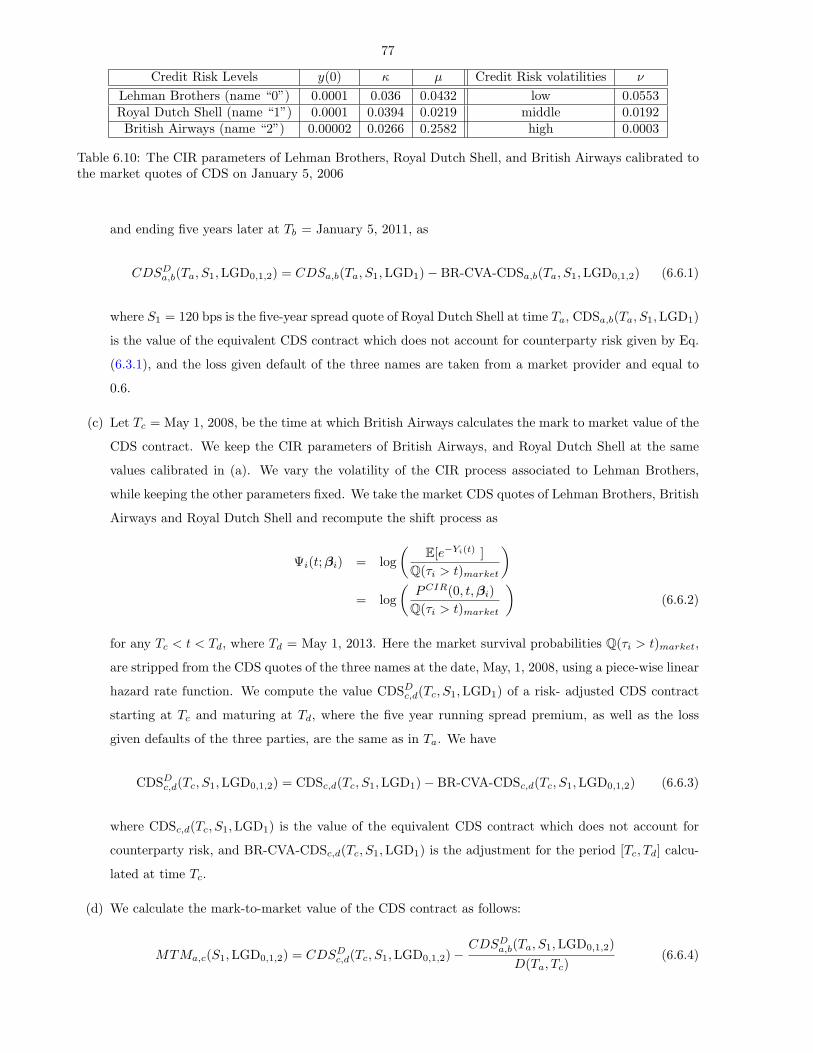
77
Credit Risk Levels y(0) κ µ Credit Risk volatilities ν
Lehman Brothers (name “0”) 0.0001 0.036 0.0432 low 0.0553Royal Dutch Shell (name “1”) 0.0001 0.0394 0.0219 middle 0.0192British Airways (name “2”) 0.00002 0.0266 0.2582 high 0.0003
Table 6.10: The CIR parameters of Lehman Brothers, Royal Dutch Shell, and British Airways calibrated tothe market quotes of CDS on January 5, 2006
and ending five years later at Tb = January 5, 2011, as
CDSDa,b(Ta, S1,LGD0,1,2) = CDSa,b(Ta, S1,LGD1)− BR-CVA-CDSa,b(Ta, S1,LGD0,1,2) (6.6.1)
where S1 = 120 bps is the five-year spread quote of Royal Dutch Shell at time Ta, CDSa,b(Ta, S1,LGD1)
is the value of the equivalent CDS contract which does not account for counterparty risk given by Eq.
(6.3.1), and the loss given default of the three names are taken from a market provider and equal to
0.6.
(c) Let Tc = May 1, 2008, be the time at which British Airways calculates the mark to market value of the
CDS contract. We keep the CIR parameters of British Airways, and Royal Dutch Shell at the same
values calibrated in (a). We vary the volatility of the CIR process associated to Lehman Brothers,
while keeping the other parameters fixed. We take the market CDS quotes of Lehman Brothers, British
Airways and Royal Dutch Shell and recompute the shift process as
Ψi(t;βi) = log(
E[e−Yi(t) ]Q(τi > t)market
)= log
(PCIR(0, t,βi)
Q(τi > t)market
)(6.6.2)
for any Tc < t < Td, where Td = May 1, 2013. Here the market survival probabilities Q(τi > t)market,
are stripped from the CDS quotes of the three names at the date, May, 1, 2008, using a piece-wise linear
hazard rate function. We compute the value CDSDc,d(Tc, S1,LGD1) of a risk- adjusted CDS contract
starting at Tc and maturing at Td, where the five year running spread premium, as well as the loss
given defaults of the three parties, are the same as in Ta. We have
CDSDc,d(Tc, S1,LGD0,1,2) = CDSc,d(Tc, S1,LGD1)− BR-CVA-CDSc,d(Tc, S1,LGD0,1,2) (6.6.3)
where CDSc,d(Tc, S1,LGD1) is the value of the equivalent CDS contract which does not account for
counterparty risk, and BR-CVA-CDSc,d(Tc, S1,LGD1) is the adjustment for the period [Tc, Td] calcu-
lated at time Tc.
(d) We calculate the mark-to-market value of the CDS contract as follows:
MTMa,c(S1,LGD0,1,2) = CDSDc,d(Tc, S1,LGD0,1,2)−CDSDa,b(Ta, S1,LGD0,1,2)
D(Ta, Tc)(6.6.4)

78
Table 6.11 reports the MTM value of the CDS contract between British Airways and Lehman Brothers on
default of Royal Dutch Shell under a number of correlation scenarios. The CDS contract agreed on January
5, 2006, is marked to market on May, 1, 2008 by British Airways using the four-step procedure described
above. We check the effect of the increasing riskiness of Lehman Brothers by varying the volatility of the
CIR process associated to Lehman. Table 6.11 reveals large sensitivity of the BR-CVA to default correlation
(r01, r02, r12) Vol νLeh 0.01 0.10 0.20 0.30 0.40 0.50CDS Implied vol 1.5% 15% 28% 37% 42% 42%
(-0.3, -0.1, 0.7) (LEH Pay, BAB Rec) -56.0(5.6) -55.7(5.7) -55.6(5.6) -55.6(5.6) -55.8(5.6) -55.6(5.7)(BAB Pay, LEH Rec) 84.2(0.0) 84.2(0.0) 84.2(0.0) 84.2(0.0) 84.2(0.0) 84.2(0.0)
(-0.1, -0.3, 0.8) (LEH Pay, BAB Rec) -41.6(9.1) -41.7(9.1) -41.7(9.1) -41.6(9.1) -41.7(9.1) -41.6(9.1)(BAB Pay, LEH Rec) 83.8(0.1) 83.8(0.1) 83.8(0.1) 83.7(0.1) 83.8(0.1) 83.8(0.1)
(0, 0, -0.5) (LEH Pay, BAB Rec) -84.2(0.0) -84.2(0.0) -84.2(0.0) -84.2(0.0) -84.2(0.0) -84.2(0.0)(BAB Pay, LEH Rec) 86.3(0.5) 86.3(0.5) 86.2(0.5) 86.2(0.5) 86.2(0.5) 86.2(0.5)
(0, 0, 0.6) (LEH Pay, BAB Rec) -62.2(3.9) -62.4(3.9) -62.4(3.9) -62.3(3.9) -62.6(3.9) -62.3(3.9)(BAB Pay, LEH Rec) 82.8(0.2) 82.8(0.2) 82.7(0.2) 82.7(0.2) 82.7(0.2) 82.7(0.2)
(0, 0, 0.9) (LEH Pay, BAB Rec) -32.4(10.9) -31.7(10.9) -31.4(10.9) -31.6(10.9) -32.8(10.9) -32.5(10.9)(BAB Pay, LEH Rec) 82.9(0.2) 82.8(0.2) 82.8(0.2) 82.8(0.2) 82.8(0.2) 82.8(0.2)
(0, 0.7, 0) (LEH Pay, BAB Rec) -81.9(0.3) -82.0(0.3) -82.0(0.3) -82.0(0.3) -82.0(0.3) -82.0(0.3)(BAB Pay, LEH Rec) 83.1(0.2) 83.1(0.2) 83.0(0.2) 83.0(0.2) 82.9(0.2) 83.0(0.2)
(0, 0.7, 0.7) (LEH Pay, BAB Rec) -53.9(6.8) -54.0(6.8) -53.4(6.8) -53.7(6.8) -53.6(6.8) -54.1(6.8)(BAB Pay, LEH Rec) 83.0(0.2) 83.0(0.2) 83.0(0.2) 82.9(0.2) 83.0(0.2) 83.0(0.2)
(0.1, 0.3, 0.8) (LEH Pay, BAB Rec) -54.6(6.4) -53.6(6.6) -54.5(6.4) -53.6(6.6) -53.8(6.6) -53.7(6.6)(BAB Pay, LEH Rec) 81.5(0.5) 81.5(0.5) 81.4(0.5) 81.4(0.5) 81.5(0.5) 81.4(0.5)
(0.25, 0.25, 0.9) (LEH Pay, BAB Rec) -39.5(10.8) -39.0(10.9) -38.6(10.9) -38.8(10.9) -40.3(10.8) -39.7(10.8)(BAB Pay, LEH Rec) 79.0(1.0) 79.0(1.0) 78.9(1.0) 78.9(1.0) 78.9(1.0) 78.9(1.0)
(0.3, 0.1, 0.7) (LEH Pay, BAB Rec) -58.7(4.6) -59.1(4.6) -58.9(4.6) -58.9(4.6) -59.3(4.6) -58.8(4.6)(BAB Pay, LEH Rec) 77.9(1.2) 77.9(1.2) 77.8(1.2) 77.9(1.2) 77.9(1.2) 77.8(1.2)
(0.5, 0.5, 0.5) (LEH Pay, BAB Rec) -68.7(2.7) -68.8(2.7) -68.7(2.7) -68.8(2.7) -69.0(2.7) -68.9(2.7)(BAB Pay, LEH Rec) 74.0(2.3) 74.0(2.3) 73.9(2.3) 74.1(2.3) 73.9(2.3) 73.9(2.3)
(0.7, 0, 0) (LEH Pay, BAB Rec) -81.3(0.3) -81.3(0.3) -81.3(0.3) -81.4(0.3) -81.2(0.3) -81.3(0.3)(BAB Pay, LEH Rec) 63.9(4.4) 64.0(4.4) 63.8(4.4) 64.2(4.4) 64.0(4.4) 63.9(4.4)
(0.7, 0, 0.7) (LEH Pay, BAB Rec) -49.6(6.5) -49.6(6.5) -49.6(6.5) -49.8(6.5) -50.0(6.5) -49.8(6.5)(BAB Pay, LEH Rec) 63.4(4.4) 63.5(4.4) 63.3(4.4) 63.8(4.4) 63.4(4.4) 63.4(4.4)
(0.9, 0.9, 0.9) (LEH Pay, BAB Rec) -44.6(9.1) -44.8(9.0) -44.5(9.1) -44.7(9.1) -44.4(9.1) -44.7(9.1)(BAB Pay, LEH Rec) 53.5(7.1) 53.4(7.1) 53.6(7.1) 53.8(7.1) 54.1(7.0) 53.8(7.1)
Table 6.11: Value of the CDS contract between British Airways and Lehman Brothers on default of RoyalDutch Shell agreed on January 5, 2006, and marked to market by British Airways on May 1, 2008. The pairs(LEH Pay, BAB Rec) and (BAB Pay, LEH Rec) denote respectively the mark-to-market value when BritishAirways is the CDS receiver and CDS payer. The mark-to-market value of the CDS contract without riskadjustment when British Airways is respectively payer (receiver) is 84.2(-84.2) bps, due to the widening ofthe CDS spread curve of Royal Dutch Shell.
and very small sensitivity to credit risk volatility of Lehman.
When Lehman is negatively correlated or uncorrelated with Royal Dutch Shell and British Airways,
which are instead positively correlated, then the likelihood of Lehman being the first to default tends to
decrease. Moreover, the value of the CDS contract at the default time is very likely to be negative because
of the copula contagion effect of Royal Dutch Shell on British Airways and of the increased five-year spread
quotes of Shell. Therefore, when Lehman is the CDS receiver, the above considerations and Eq. (6.2.4) show
that the Lehman BR-CVA becomes negligible and consequently the mark-to-market value of the contract
equals its non-risk-adjusted counterpart. Conversely, when Lehman is the payer, then the default of British
Airways is associated with a positive CDS contract value for Lehman at the default time. Eq. (6.2.4)
thus implies that the value of the CDS contract for the investor Lehman gets reduced and consequently the
mark-to-market value of the CDS contract for British Airways gets increased.
We next invert the role of Lehman Brothers and Royal Dutch Shell, hence Royal Dutch Shell becomes
the investor and Lehman Brothers the reference entity. This is a natural case to examine in that the CVA
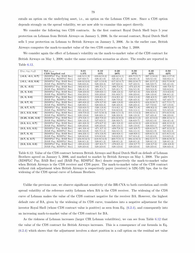
79
entails an option on the underlying asset, i.e., an option on the Lehman CDS now. Since a CDS option
depends strongly on the spread volatility, we are now able to examine this aspect directly.
We consider the following two CDS contracts. In the first contract Royal Dutch Shell buys 5 year
protection on Lehman from British Airways on January 5, 2006. In the second contract, Royal Dutch Shell
sells 5 year protection on Lehman to British Airways on January 5, 2006. As in the earlier case, British
Airways computes the mark-to-market value of the two CDS contracts on May 1, 2008.
We consider again the effect of Lehman’s volatility on the mark-to-market value of the CDS contract for
British Airways on May 1, 2008, under the same correlation scenarios as above. The results are reported in
Table 6.12.
(r01, r02, r12) Vol νLeh 0.01 0.10 0.20 0.30 0.40 0.50CDS Implied vol 1.5% 15% 28% 37% 42% 42%
(-0.3, -0.1, 0.7) (RDSPLC Pay, BAB Rec) -448.5(11.9) -433.6(13.2) -422.6(14.1) -403.7(15.7) -387.1(16.6) -364.1(17.8)(BAB Pay, RDSPLC Rec) 527.0(0.7) 526.3(1.0) 525.2(1.2) 524.9(1.3) 523.5(1.6) 522.0(2.1)
(-0.1, -0.3, 0.8) (RDSPLC Pay, BAB Rec) -440.3(12.6) -427.1(13.9) -417.3(14.7) -393.2(16.7) -381.2(17.2) -352.7(18.9)(BAB Pay, RDSPLC Rec) 528.6(0.2) 528.3(0.3) 527.6(0.5) 527.4(0.5) 526.5(0.7) 525.4(1.0)
(0, 0, -0.5) (RDSPLC Pay, BAB Rec) -502.0(3.4) -495.7(4.1) -486.7(4.8) -473.2(5.9) -460.7(6.8) -440.7(8.5)(BAB Pay, RDSPLC Rec) 526.2(1.2) 525.4(1.7) 525.2(1.7) 524.5(1.9) 523.5(2.3) 522.6(2.6)
(0, 0, 0.6) (RDSPLC Pay, BAB Rec) -529.2(0.0) -529.0(0.1) -528.1(0.4) -527.0(1.0) -524.3(0.8) -513.6(2.0)(BAB Pay, RDSPLC Rec) 534.2(0.5) 533.2(0.6) 531.8(0.7) 530.2(0.6) 528.1(0.8) 526.8(1.2)
(0, 0, 0.9) (RDSPLC Pay, BAB Rec) -523.6(0.5) -519.8(1.0) -514.9(1.4) -510.1(1.6) -500.4(2.5) -489.7(3.1)(BAB Pay, RDSPLC Rec) 529.0(0.1) 528.8(0.1) 528.7(0.2) 528.4(0.3) 527.9(0.5) 527.4(0.7)
(0, 0.7, 0) (RDSPLC Pay, BAB Rec) -485.6(6.2) -476.5(7.0) -466.1(8.0) -450.8(9.5) -434.9(10.7) -417.7(11.7)(BAB Pay, RDSPLC Rec) 528.9(0.1) 528.6(0.3) 528.4(0.3) 528.2(0.4) 527.7(0.6) 527.1(0.8)
(0, 0.7, 0.7) (RDSPLC Pay, BAB Rec) -523.6(0.5) -520.1(0.8) -514.6(1.4) -508.7(1.8) -499.9(2.3) -488.5(3.0)(BAB Pay, RDSPLC Rec) 521.3(3.0) 519.7(3.7) 518.8(3.8) 518.1(4.1) 516.6(4.6) 515.3(5.0)
(0.1, 0.3, 0.8) (RDSPLC Pay, BAB Rec) -459.7(9.2) -447.5(10.3) -436.1(11.5) -415.1(13.2) -399.3(14.1) -374.0(15.8)(BAB Pay, RDSPLC Rec) 529.1(0.0) 528.8(0.1) 528.3(0.3) 528.1(0.3) 527.4(0.4) 526.2(0.8)
(0.25, 0.25, 0.9) (RDSPLC Pay, BAB Rec) -473.5(8.1) -463.7(9.2) -453.3(10.0) -436.6(11.6) -421.2(12.6) -398.2(14.1)(BAB Pay, RDSPLC Rec) 528.1(0.3) 527.6(0.5) 526.9(0.7) 526.6(0.7) 525.6(1.0) 524.4(1.4)
(0.3, 0.1, 0.7) (RDSPLC Pay, BAB Rec) -481.6(6.3) -472.6(7.2) -461.5(8.2) -443.4(10.2) -430.2(10.6) -408.2(12.2)(BAB Pay, RDSPLC Rec) 529.2(0.0) 529.2(0.0) 529.1(0.1) 529.1(0.0) 528.8(0.1) 527.8(0.4)
(0.5, 0.5, 0.5) (RDSPLC Pay, BAB Rec) -481.3(6.4) -471.3(7.3) -459.7(8.3) -445.3(9.7) -429.6(10.7) -407.2(12.2)(BAB Pay, RDSPLC Rec) 526.5(0.8) 525.7(1.2) 524.5(1.5) 524.1(1.5) 522.6(1.9) 521.0(2.3)
(0.7, 0, 0) (RDSPLC Pay, BAB Rec) -484.2(6.1) -474.1(6.9) -463.6(8.1) -449.9(9.1) -429.0(11.3) -415.8(11.6)(BAB Pay, RDSPLC Rec) 520.8(3.0) 519.0(3.8) 518.0(3.9) 517.0(4.2) 515.2(4.8) 513.6(5.2)
(0.7, 0, 0.7) (RDSPLC Pay, BAB Rec) -434.9(12.5) -418.9(14.0) -403.7(15.1) -384.4(16.5) -362.5(17.7) -338.6(19.3)(BAB Pay, RDSPLC Rec) 528.0(1.2) 528.0(1.2) 528.0(1.2) 528.0(1.2) 528.0(1.2) 528.0(1.2)
(0.9, 0.9, 0.9) (RDSPLC Pay, BAB Rec) -495.6(4.0) -487.8(4.7) -479.0(5.4) -458.5(7.7) -448.5(7.6) -430.4(8.9)(BAB Pay, RDSPLC Rec) 529.2(0.0) 529.2(0.0) 529.1(0.0) 529.2(0.0) 529.2(0.0) 528.0(0.4)
Table 6.12: Value of the CDS contract between British Airways and Royal Dutch Shell on default of LehmanBrothers agreed on January 5, 2006, and marked to market by British Airways on May 1, 2008. The pairs(RDSPLC Pay, BAB Rec) and (BAB Pay, RDSPLC Rec) denote respectively the mark-to-market valuewhen British Airways is the CDS receiver and CDS payer. The mark-to-market value of the CDS contractwithout risk adjustment when British Airways is respectively payer (receiver) is 529(-529) bps, due to thewidening of the CDS spread curve of Lehman Brothers.
Unlike the previous case, we observe significant sensitivity of the BR-CVA to both correlation and credit
spread volatility of the reference entity Lehman when BA is the CDS receiver. The widening of the CDS
curve of Lehman makes the value of the CDS contract negative for the receiver BA. However, the highest
default rate of BA, given by the widening of its CDS curve, translates into a negative adjustment for the
investor Royal Shell (whose CDS contract value is positive) as seen from Eq. (6.2.4), and consequently into
an increasing mark-to-market value of the CDS contract for BA.
As the riskness of Lehman increases (larger CIR Lehman volatilities), we can see from Table 6.12 that
the value of the CDS contract for British Airways increases. This is a consequence of our formula in Eq.
(6.2.4) which shows that the adjustment involves a short position in a call option on the residual net value
80
of the Lehman CDS portfolio evaluated at the time when BA defaults and a long position in a default put
option on the residual net value of the Lehman CDS portfolio evaluated at the time when Shell defaults.
Given that options increase with volatility and that the event of BA defaulting is more likely than the event
of Shell defaulting because of the wider BA CDS term structure, we have that the short position in the call
option is the driving factor of the adjustment, and it lowers the value of the risk-adjusted CDS contract for
Shell as the underlying Lehman CIR volatility increases.
6.7 Conclusions
In this chapter we have provided a general arbitrage-free framework for calculating the bilateral counterparty
credit valuation adjustment (BR-CVA) for payoffs exchanged between two parties, an investor and her
counterparty. First, we have provided a general formula for computing the BR-CVA of financial contracts
which are traded over-the-counter. Then, we have specialized our analysis to the case where also the
underlying portfolio is sensitive to a third credit event, and in particular to the case where the underlying
portfolio is a credit default swap on a third entity. We have then developed a Monte-Carlo numerical scheme
to evaluate the formula and thus compute the BR-CVA in the specific case of credit default swap contracts.
The Monte-Carlo scheme combines Fourier transform methods with filtration switching formulas and provides
an efficient algorithm for numerically evaluating the adjustment. We have provided a case study in Section
6.5, and experimented with different levels of credit risk and credit risk volatilities of the three names as
well as with different scenarios of default correlation. The results obtained confirm that the adjustment
is sensitive to both default correlation and credit spreads volatility, having richly structured patterns that
cannot be captured by rough multipliers. This points out that attempting to adapting the capital adequacy
methodology (Basel II) to evaluating wrong-way risk by means of rough multipliers is not feasible. Our
analysis confirms that also in the bilateral-symmetric case, wrong-way risk —namely the supplementary risk
that one undergoes when the correlation assumes the worst possible value— has a structured pattern that
cannot be captured by simple multipliers applied to the zero correlation case.

81
Chapter 7
Conclusions
7.1 Concluding Remarks
This thesis extends the credit risk literature along two main directions
• Credit Risk Modeling: It proposes a new credit risk framework for modeling deliberate distortion of
the reported firm’s asset values. The distortion is applied by insiders of the firm such as managers,
and is not directly observable by the outside market which can only infer it from available data. The
amount of distortion depends on the current performance of the firm and it also has implications on
the future management of the firm.
• Counterparty risk valuation: It provides a general framework for calculating the bilateral counterparty
credit valuation adjustment (BR-CVA) for payoffs exchanged between two parties, an investor and her
counterparty, both bearing risk of default.
After an introduction to credit risk modeling and basic preliminaries presented in Chapters 1 and 2,
Chapter 3 presents the theory underlying the proposed credit model. It describes its building blocks and
derives explicit and computable expressions for bond and equity prices, conditional default probability,
recovery rate, and credit spreads.
The estimate of the log-asset value of the firm in the proposed model is a crucial quantity for determining
the price of corporate securities. The mathematical framework of our credit model, namely a jump linear
system with state-dependent transition probabilities, leads to solving a nonlinear filtering problem evaluating
the conditional density of the asset value. The problem is computationally untractable since the conditional
log-asset value filter density would require an exponentially increasing number of terms. In order to deal
with the exploding computational complexity, we have proposed in Chapter 5 a novel methodology which
approximates the actual log-asset value density with a Gaussian mixture. Such methodology selects the
smallest possible number of Gaussian components which approximate the true density within a desired level
of accuracy through the solution of a second-order cone programming problem.
Chapter 4 shows the power of the proposed model in dealing with real situations of misreporting. It
first introduces a novel estimation procedure for a simplified version of our model and then applies it to
the Parmalat case. Such estimation procedure implies the market observations of the reported log-asset

82
value, instead of the actual log-asset value which is only known to insiders, from equity prices. The obtained
results are in line with the existing findings in the literature, and (a) confirm the importance of modeling
accounting distortion in credit risk models, and (b) evidence that its omission may result in exaggeratedly
large estimates of asset volatility.
Chapter 6 addresses the problem of bilateral risk evaluation in over-the-counter contracts. It develops a
general arbitrage-free framework and specializes the analysis to the case where also the underlying portfolio
is sensitive to a third credit event, and in particular to the case where the underlying portfolio is a credit
default swap on a third entity. It develops a Monte-Carlo numerical scheme to evaluate the formula and
computes the BR-CVA in the specific case of credit default swap contracts. It proposes case studies to
measure the impact of both default correlation and credit spreads volatility on the adjustment, and shows
that they both have a significant impact on the adjustment evaluation, thus adding to the existing literature,
which only measures the impact of default correlation on the adjustment.
7.2 Future Work
There are several directions which we can follow to extend and improve the results of this thesis. We next
outline some of them.
• Model endogenization. It would be interesting to define an optimal level of debt K∗ and an equity
maximizing bankruptcy trigger B < K∗ at which shareholders’s incentives to continue operating the
firm’s assets vanish.
• Dynamic consequences of accounting transparency. We could look at the dynamic implications of
misreporting on the future evolution of asset value. This would require formulating misreporting
as an optimal controlled diffusion problem with partial information. The bias to the asset value
added by the managers would be optimally chosen in such a way as to maximize their utility function
at some time horizon. Although some work on analytical methods for controlled diffusion process
with partial information has been done, see Bjork et al. (2008) and Haussmann and Sass (2004),
those techniques would not be able to handle our credit risk framework. There would be a need to
develop efficient numerical methods combining statistical Bayesian filtering with utility maximization
methods.Additional challenges would be posed by the calibration of those models. Currently, all
calibrations use a constant and exogenous value for asset volatility and reporting bias, thus a new
calibration methodology would be needed to handle the new scenario.
• Hedging of credit risk. The problem of credit risk hedging is very relevant and important nowadays
due to the high numbers of credit rating downgrading or even default events being experienced. The
challenge would be the construction of an appropriate model in which a family of options written on
credit- sensitive instruments can be valued and hedged. Some efforts, although at a very abstract level
start appearing Bielecki et al. (2008).

83
Bibliography
E. Altman, A. Resti, and A. Sironi. Analyzing and explaining default recovery rates. Technical Report: The
International Swaps and Derivatives Association, 2000. 25
P. Artzner and F. Delbaen. Default risk insurance and incomplete markets. Mathematical Finance, 5:
187–195, 1995. 11
Y. Bar-Shalom, X.R. Li, and T. Kirubarajan. Estimation with Applications to Tracking and Navigation.
John Wiley & Sons, 2002. 42
T. Bielecki, M. Jeanblanc, and M. Rutkowski. Hedging of credit default swaptions in a hazard process model.
Working paper, available at http://www.defaultrisk.com/pp crdrv169.htm, December 2008. 82
T. Bjork, M. Davis, and C. Landen. Optimal investment under partial information. Preprint, 2008. 82
F. Black and J. Cox. Valuing corporate securities: some effects of bond indenture provisions. Journal of
Finance, 31:351–367, 1976. 6
H. Blom and Y. Bar-Shalom. The interacting multiple model algorithm for systems with Markovian switching
coefficients. IEEE Transaction on Automatic Control, 33:780–783, 1988. 43, 52
H. Blom and E. Bloem. Exact Bayesian and particle filtering of stochastic hybrid systems. IEEE Transactions
on Aerospace and Electronic Systems, 43:55–70, 2007. 44
D. Brigo. Counterparty risk valuation with stochastic dynamical models: Impact of volatilities and cor-
relations. In Proceedings of 5th World Business Strategies Fixed Income Conference, September 2008.
63
D. Brigo and A. Alfonsi. Credit default swap calibration and derivatives pricing with the ssrd stochastic
intensity model. Finance and Stochastics, 9:29–42, 2005. 66
D. Brigo and A. Capponi. Bilateral counterparty risk with application to cds. Submitted to Risk Magazine.
(Submission Date: January 26, 2009). 4
D. Brigo and K. Chourdakis. Counterparty risk for credit default swaps: Impact of spread volatility and
default correlation. Working paper, Fitch solutions, 2008. 60, 65, 68, 72
D. Brigo and N. El-Bachir. An exact formula for default swaptions’ pricing in the ssrjd stochastic intensity
model. Mathematical Finance, 2008. 60, 66, 67

84
D. Brigo and M. Masetti. Counterparty Credit Risk Modeling: Risk Management, Pricing and Regulation,
chapter 10, Risk Neutral Pricing of Counterparty Risk. Risk Books, London, 2005. 60
D. Brigo and F. Mercurio. Interest Rate Models: Theory and Practise —with Smile, Inflation and Credit.
Springer Verlag, 2nd edition, 2006. 59, 66, 68, 71
D. Brigo and M. Morini. Cds calibration with tractable structural models under uncertain credit quality.
Risk Magazine, 19, 2006. 15, 32
D. Brigo and A. Pallavicini. Numerical Methods for Finance, chapter Counterparty Risk under Correlation
between Default and Interest Rates. Chapman Hall, 2007. 60
D. Brody, L. Hughston, and A. Macrina. Beyond hazard rates: a new approach to credit risk modelling.
In Advances in Mathematical Finance, volume in honour of D. Madan, pages 231–257. Birkhuser and
Springer, 2007. 13
D. Brody, L. Hughston, and A. Macrina. Information-based asset pricing. International Journal of Theoretical
and Applied Finance, 11:107–142, 2008. 13
E. Canabarro and D. Duffie. Credit risk for otc derivatives portfolios: Exposure and valuation. ALM of
Financial Institutions, Institutional Investor Books ed. Leo Tilman, 2004. 59
A. Capponi. A convex optimization approach to filtering in jump systems with state dependent transition
probabilities. Forthcoming in Automatica Elsevier, 2009a. 4
A. Capponi. A calibration method for structural models of credit risk with reporting bias. In Proceedings
of the IEEE Conference on Computational Intelligence in Financial Engineering, 2009b. 4
A. Capponi and J. Cvitanic. Credit risk modelling with misreporting and incomplete information. Interna-
tional Journal of Theoretical and Applied Finance, 12:83–112, 2009. 3
U. Cetin, R. Jarrow, P. Protter, and Y. Yildirim. Modeling credit risk with partial information. Annals of
Applied Probability, 14:1167–1178, 2004. 13
S. Chen, D. Donoho, and M. Saunders. Atomic decomposition by basis pursuit. SIAM Review, 43:129–159,
2001. 46
U. Cherubini and M. Manera. Hunting the living dead: A peso problem in corporate liabilities data. ICFAI
Journal of Financial Risk Management, 3:44–56, 2006. 15, 32
U. Cherubini, E. Luciano, and W. Vecchiato. Copula Methods in Finance. Wiley Finance, 2004. 65
K. Chourdakis. Option pricing using the fractional fft. Journal of Computational Finance, 8:1–18, 2005. 69
D. Coculescu, H. Geman, and M. Jeanblanc. Valuation of default sensitive claims under imperfect informa-
tion. Finance and Stochastics, 12:195–218, 2008. 20
85
P. Collin-Dufresne, R. Goldstein, and J. Hugonnier. A general formula for pricing defaultable securities.
Econometrica, 72:1377–1407, 2004. 6, 60
J. Cox, J. Ingersoll, and S. Ross. A theory of the term structure of interest rates. Econometrica, 53:385–408,
1985. 66
D. Donoho and M. Elad. Maximal sparsity representation via l1 minimization. Proceedings of National
Academy of Sciences, 100:2197–2202, 2003. 46
A. Doucet, N. Gordon, and V. Krishnamurthy. Particle filters for state estimation of jump Markov linear
systems. IEEE Transactions on Signal Processing, 49:613–624, 2001. 43
J. Duan. Correction: Maximum likelihood estimation using price data of the derivative contract. Mathe-
matical Finance, 10:461–462, 2000. 29
J. Duan. Maximum likelihood estimation using price data of the derivative contract. Mathematical Finance,
4:155–167, 1994. 29
D. Duffie and M. Huang. Swap rates and credit quality. Journal of Finance, 51:921–950, 1996. 60
D. Duffie and D. Lando. Term structure of credit spreads with incomplete accounting information. Econo-
metrica, 63:633–664, 2001. 13, 15, 27
D. Duffie and K. Singleton. Modeling term structures of defaultable bonds. Review of Financial Studies, 12:
687–720, 1999. 11
Y. Eom, J. Helwege, and J. Huang. Structural models of corporate bond pricing: An empirical analysis.
Review of Financial Studies, 17:499–544, 2003. 29
P. Fisher and R. Verrecchia. Reporting bias. The Accounting Review, 75:229–245, 2000. 15
R. Frey and W. Runggaldier. Credit risk and incomplete information: a nonlinear-filtering approach.
Preprint, 2007. 13
R. Geske. The valuation of corporate liabilities as compound options. Journal of Financial and Quantitative
Analysis, 12:541–552, 1977. 6
K. Giesecke and L. R. Goldberg. Forecasting default in the face of uncertainty. Journal of Derivatives, 12:
11–25, 2004. 13
M. Grant and S. Boyd. Graph implementations for nonsmooth convex programs. In Recent Advances in
Learning and Control, Lecture Notes in Control and Information Sciences, pages 95–110. Springer, 2008.
54
X. Guo, R. A. Jarrow, and Y. Zeng. Credit risk models with incomplete information. Forthcoming in
Mathematics of Operations Research, 2009. 13

86
U. Haussmann and J. Sass. Optimizing the terminal wealth under partial information: The drift process as
a continuous time markov chain. Finance and Stochastics, 8:553–577, 2004. 82
J. Huang and M. Huang. How much of the corporate-treasury yield spread is due to credit risk? Working
paper, Pennsylvania State and Stanford Universities, 2003. 29
J. Hull and A. White. Valuing credit default swaps: Modeling default correlations. Working paper, University
of Toronto, 2000. 60
R. Jarrow and S. Turnbull. Pricing derivatives on financial securities subject to credit risk. Journal of
Finance, 50:53–86, 1995. 11
M. Jeanblanc and M. Rutkowski. Mathematical Finance: Theory and Practise, volume 1, chapter Modeling
Default Risk: An Overview, pages 71–269. Higher Education Press, Beijing, 2000. 20
I. Karatzas and S. Shreve. Brownian Motion and Stochastic Calculus. (Graduate Texts in Mathematics).
Springer-Verlag, New York, 1995. 9
D. Lando. Credit Risk Modeling: Theory and Applications. Princeton University Press, 2004. 5
H. E. Leland. Prediction of default probabilities in structural models of debt. Journal of Investment
Management, 2:5–20, 2004. 29
H. E. Leland and K. Toft. Optimal capital structure, endogeneous bankruptcy, and the term structure of
credit spreads. Journal of Finance, 51:987–1019, 1996. 6
X. Rong Li and V. P. Jilkov. A survey of maneuvering target tracking: Multiple-model methods. IEEE
Transactions on Aerospace and Electronic Systems, 41:1255–1321, 2005. 43
M. Lobo, L. Vanderberghe, S. Boyd, and H. Lebret. Applications of second-order cone programming. Linear
Algebra and its Applications, 284:193–228, 1998. 53
F. Longstaff and E. Schwartz. A simple approach for valuing risky fixed and floating rate debt. Journal of
Finance, 50:789–819, 1995. 6
R. C. Merton. On the pricing of corporate debt: the risk structure of interest rates. Journal of Finance, 29:
449–470, 1974. 6
R. Nelsen. An Introduction to Copulas. Springer Verlag, 2006. 65
W. J. Runggaldier. Mathematics of Finance (G.Yin and Q.Zhang eds.), volume 351, chapter Estimation
via stochastic filtering in financial market models, pages 309–318. Contemporary Mathematics, America
Mathematical Society, 2004. 21
P. Schonbucher. Credit derivatives pricing models: Models, Pricing, Implementation. Wiley Finance, 2003.
109

87
T. Wang. Real investment and corporate securities fraud. Working paper, University of Minnesota, 2007.
16, 17, 18
F. Yu. Accounting transparency and the term structure of credit spreads. Journal of Financial Economics,
75:53–84, 2005. 15
C. Zhou. The term structure of credit spreads with jump risk. Journal of Banking and Finance, 25:2015–2040,
2001. 12

88
Appendix A
Chapter 3: Bond and Equity Prices
We recall from Section 3.4 that the time t price of a bond with maturity T is given by
B(t, T ) = e−rτ (K − EP∗[(K − VT )+|F z
t ]) (A.0.1)
Following the assumptions made in Section 3.4.3 the probability measure P ∗ is obtained replacing µ with
r and assuming that the biases h(i) and the accounting risks ν(i) are the same under the historical and
risk-neutral measure. We then have
E[e−rτ (K − VT )+|F zt ] = e−rτ
∫R
∫R
P (xT = x|xt = y)pt|t(y)(K − ex)+dydx
= e−rτ∫R
pt|t(y)∫R
P (xT = x|xt = y)(K − ex)+dxdy (A.0.2)
where we have used the assumption made in Section 3.4.3 that the volatility risk σ(l) is mode independent.
The inner integral can be explicitly computed since P (xT = x|xt = y) is a Gaussian density with mean
µy = y + (r − 0.5σ2)τ and variance σ2τ , thus
∫R
P (xT = x|xt = y)(K − ex)+dx = Enµy,σ2τ[(K − eX)+] (A.0.3)
where nµy,σ2τ denotes the Gaussian density with mean µy and variance σ2τ and X is a random variable
with density nµy,σ2τ .
We have
Enµy,σ2τ[(K − eX)+] = Enµy,σ2τ
[K1K≥eX]− Enµy,σ2τ[eX1K≥eX]
:= I1 − I2 (A.0.4)
It is easy to see that I1 is given by:
I1 = KN(−d2(y))

89
where d2(y) =µy − log(K)
σ√τ
. We compute I2 as:
I2 =∫ −d2(y)
−∞expµy + σ
√τzn(z)dz
= ey+rτ1√2π
∫ −d2(y)
−∞exp−0.5(z − σ
√τ)2dz
= ey+rτN(−d1(y)) (A.0.5)
where d1(y) = d2(y) + σ√τ . Therefore,
En(x;µy,σ2τ)[(K − ex)+] = KN(−d2(y))− ey+rτN(−d1(y)) (A.0.6)
Thus, we have that
E[e−rτ (K − VT )+|F zt ] = Ept|t [Ke
−rτN(−d2(Y ))− eYN(−d1(Y ))] (A.0.7)
where Y is a random variable with density pt|t and the price of the bond is then given by
B(t, T ) = Ke−rτ − Ept|t [Ke−rτN(−d2(Y ))− eyN(−d1(Y ))] (A.0.8)

90
Appendix B
Chapter 3: Approximate Bond andEquity Prices
We recall from Section 3.5.1 that the price of the bond at time t is given by
B(t, T ) = e−rτ
K −∑j
µjtE[(K − V jT |t)+]
(B.0.1)
where V jT |t is the exponential of a Gaussian random variable with mean xjT |t = xjt|t + (r − 0.5σ2)τ and
standard deviation σjT |t =√σ2,jt|t + σ2τ . We have
E[(K − V jT |t)+] = E[K1K≥V j
T |t]− E[V jT |t1K≥V j
T |t]
:= Ij1 − Ij2 (B.0.2)
It is easy to see that Ij1 is given by:
Ij1 = KP
N(0, 1) ≤log(K)− xjt|t − (r − 0.5σ2)τ√
σ2,jt|t + σ2τ
= KN(−dj2) (B.0.3)
where dj2 =xjt|t − log(K) + (r − 0.5σ2)τ√
σ2,jt|t + σ2τ
. The expression for Ij2 is given by:
Ij2 =∫ −dj
2
−∞exp
xjt|t + (r − 0.5σ2)τ +
√σ2,jt|t + σ2τz
n(z)dz
= expxjt|t + 0.5σ2,jt|t + rτ 1√
2π
∫ −dj2
−∞exp
−0.5
(z −
√σ2,jT |t + σ2τ
)2dz
= expxjt|t + 0.5σ2,jt|t + rτN(−dj1) (B.0.4)
where dj1 = dj2 +√σ2,jt|t + σ2τ . Thus
E[e−rτ (K − V jT |t)+] = Ke−rτN(−dj2)− expxjt|t + 0.5σ2,j
t|t N(−dj1) (B.0.5)

91
Therefore, plugging Eq. (B.0.5) into Eq. (B.0.1), we have that the bond price is given by
B(t, T ) = Ke−rτ −∑j
µjt (Ke−rτN(−dj2)− expxjt|t + 0.5σ2,j
t|t N(−dj1)) (B.0.6)

92
Appendix C
Chapter 3: Bivariate Integrals
It is possible to establish a relation between integrals of the form
∫ xL
−∞eaxN(bx+ c)n(x)dx (C.0.1)
for some constants a, b, c and the bivariate normal distribution function. This is done as follows:
∫ xL
−∞eaxN(bx+ c)n(x)dx
=∫ xL
−∞
∫ c
−∞eaxn(bx+ y)n(x)dydx
=e0.5a
2
2π
∫ xL
−∞
∫ c
−∞e−
(1+b2)(x−a)2
2 − (y+ab)2
2 −b(y+ab)(x−a)dydx (C.0.2)
This can be related to the bivariate normal distribution as follows:
B(a, b, c) :=∫ xL
−∞eaxN(bx+ c)n(x)dx = e0.5a
2P(X ≤ xL, Y ≤ c) (C.0.3)
where (X,Y ) has a bivariate normal distribution with
µX = a, µY = −ab, σ2x = 1, σ2
j = 1 + b2, ρ = − b√1 + b2
(C.0.4)

93
Appendix D
Chapter 3: Probability of Default
Set l = r − 0.5σ2. Then, we have
PD(t, T ) = P(VT ≤ K|Vt ≥ K,F zt )
=P(VT ≤ K,Vt ≥ K|F z
t )P(Vt ≥ K|F z
t )
=P(XT ≤ log(K), Xt ≥ log(K)|F z
t )P(Xt ≥ log(K)|F z
t )
=P(lτ + σN(0, τ) ≤ −Xt + log(K), Xt > log(K)|F z
t )P(Xt ≥ log(K)|F z
t )(D.0.1)
where the last equality follows because we can decompose XT = Xt + N(lτ, σ2τ) as it can be easily checked.
Denote ddjt =xjt|t − log(K)
σjt|t. Developing the probability (D.0.1) using the associated density functions, we
obtain that the denominator is given by:
P(Xt ≥ log(K)|F zt ) = 1−
m∑j=1
µjtN(−ddjt ) =m∑j=1
µjtN(ddjt ) (D.0.2)
while the numerator P(lτ + σN(0, τ) ≤ −Xt + log(K), Xt > log(K)|F zt ) can be computed as follows:
=∫ ∞
log(K)
( m∑j=1
µjtn(x; xjt|t, σ2,jt|t ))(∫ −x+log(K)
−∞n(y; lτ, σ2τ)dy
)dx
=m∑j=1
µjt
∫ ∞
log(K)
n(x; xjt|t, σ2,jt|t )N
(−x+ log(K)− lτ
σ√τ
)dx
=m∑j=1
µjt
∫ ∞
log(K)
σjt|tn
(x− xjt|t
σjt|t
)N
(−x+ log(K)− lτ
σ√τ
)dx
=m∑j=1
µjt
∫ ddjt
−∞n(y)N
(yσjt|t − xjt|t + log(K)− lτ
σ√τ
)dy (D.0.3)

94
where the last line follows from a change of variable y =xjt|t − x
σjt|t. Using the result in Appendix C, we can
conclude that the numerator is a convex combination of bivariate cumulative distribution functions, i.e.,
P(VT ≤ K,Vt ≥ K|F zt ) =
m∑j=1
µjtP(Xj ≤ ddjt , Yj ≤ −d2(xjt|t)) (D.0.4)
where ddjt =xjt|t − log(K)
σjt|t, d2 is the function defined in Eq. (3.4.12), and (Xj , Yj) has a bivariate normal
distribution function with positive correlation ρXjYj:
µXj = µYj = 0, σ2Xj
= 1, σ2Yj
= 1 +σ2,jt|t
σ2τ, ρXjYj
=σjt|t√
σ2τ + σ2,jt|t
(D.0.5)
Defining wjt =µjtN(ddjt )∑mi=1 µ
itN(ddit)
, we obtain
PD(t, T ) =∑j
wjtP(Yj ≤ −d2(xjt|t)|Xj ≤ ddjt ) (D.0.6)

95
Appendix E
Chapter 3: Recovery Rate
Set l = (r − 0.5σ2), Zτ = lτ + σN(0, τ). We have
RR(t, T ) :=1KE[VT |VT < K,Vt > K,F z
t ]
=1KE[eXt+Zτ |Xt > log(K), Zτ < log(K)−Xt,F
zt ]
=
∫∞log(K)
ex∫ log(K)−x−∞ elτ+σ
√τyn(y)dy
∑mj=1 µ
jtn(x; xjt|tσ
2,jt|t )dx
P(Xt + Zτ < log(K), Xt > log(K)|F zt )
(E.0.1)
The denominator can be decomposed as follows:
P(Xt + Zτ < log(K), Xt > log(K)|F zt ) = PD(t, T )P (Xt > log(K)|F z
t ) (E.0.2)
where both of the quantities above have been computed in Appendix D. The numerator in the last line of
Eq. (E.0.1) can be written as:
= erτm∑j=1
µjt
∫ ∞
log(K)
exn(x; xjt|t, σ2,jt|t )N
(log(K)− x− lτ − σ2τ
σ√τ
)dx (E.0.3)
= erτm∑j=1
µjtexj
t|t
∫ ddjt
−∞e−yσj
t|tn(y)N(−xjt|t + yσjt|t + log(K)− lτ − σ2τ
σ√τ
)dy
where ddjt =xjt|t − logK
σjt|t. The last line of the derivation above follows from the change of variable y =
xjt|t − x
σjt|t. Using the result in Appendix C, we obtain that the numerator is again a convex combination of
bivariate Gaussian cumulative distribution functions given by
erτm∑j=1
µjtexj
t|t+0.5σ2,jt|t P(ξj ≤ ddjt , ψj ≤ −d1(x
jt|t)) (E.0.4)

96
where d1 is the function defined in Eq. (3.4.12), and (ξj , ψj) is a bivariate Gaussian with negative correlation
coefficient ρξjψj :
µξj = −σjt|t, µψj =σ2,jt|t
σ√τ, σ2ξj
= 1, σ2ψj
= 1 +σ2,jt|t
σ2τ, ρξjψj = −
σjt|t√σ2τ + σ2,j
t|t
(E.0.5)
Defining wjt =µjtP(Xj ≤ ddjt , Yj ≤ −d2(x
jt|t))∑m
i=1 µitP(Xi ≤ ddit, Yi ≤ −d2(xit|t))
, we obtain
RR(t, T ) = erτm∑j=1
wjtexj
t|t+σ2,jt|t2
K
P(ξj ≤ ddjt , ψj ≤ −d1(xjt|t))
P(Xj ≤ ddjt , Yj ≤ −d2(xjt|t))
(E.0.6)

97
Appendix F
Chapter 5: Facts about LipschitzFunctions
The lp norm of an n dimensional vector x is defined as follows:
||x||p =
[∑
i |xi|p] 1
p
1 ≤ p <∞
maxi=1,...n |xi| p = ∞
Lemma F.1. Let f : Rn → R. ∀x1,x2 it holds that
|f(x1)− f(x2)| ≤ Cp||x1 − x2||q (F.0.1)
where Cp = supx ||∇f(x)||p, ∇f(x) = ( ∂f∂x1, . . . , ∂f∂xn
) and 1p + 1
q = 1, 1 ≤ p, q ≤ ∞.
We next state an obvious result as a lemma. Such result states that the product of two bounded Lipschitz
functions is a bounded Lipschitz function.
Lemma F.2. Let f : Rn → R and g : Rn → R. Let Cf,p,Mf , Cg,p,Mg constants such that for all
x1,x2 ∈ Rn, we have
|f(x1)− f(x2)| ≤ Cf,p||x1 − x2||p
|g(x1)− g(x2)| ≤ Cg,p||x1 − x2||p (F.0.2)
and
|f(x)| ≤Mf
|g(x)| ≤Mg (F.0.3)
Then,
|f(x1)g(x1)− f(x2)g(x2)| ≤ (MfCg,p +MgCf,p)||x1 − x2||p (F.0.4)

98
Appendix G
Chapter 5: Total Variation distanceat initial time
Using approximation (5.3.27), we can write
||pl1,1(x)− pl1,1(x)||1 ≈∫G
|pl1,1(x)− pl1,1(x)|dx (G.0.1)
Since the vectors in the training set are equally spaced in G, we can partition G into n-dimensional cubes
and denote by Gi the n-dimensional cube in the partition having xi as the bottom left vertex of the cube.
Using the triangular inequality, we have
∫G
|pl1,1(x)− pl1,1(x)|dx
=q∑i=1
∫Gi
|pl1,1(x)− pl1,1(x)|dx
≤q∑i=1
∫Gi
|pl1,1(x)− pl1,1(xi)|dx
+∫Gi
|pl1,1(xi)− pl1,1(xi)|dx
+∫Gi
|pl1,1(xi)− pl1,1(x)|dx (G.0.2)
Next, we analyze separately the three terms in Eq. (G.0.2). The first term is upper bounded as follows
∫Gi
|pl1,1(x)− pl1,1(xi)|dx
=∫Gi
∣∣∣∣ ∫Rn
P (x0 = y)λl(y)
·(Ll1|1(x)p(x|y, l)− Ll1|1(xi)p(xi|y, l)dy)∣∣∣∣dx
≤∫Rn
P (x0 = y)λl(y)
·∫Gi
|Ll1|1(x)p(x|y, l)− Ll1|1(xi)p(xi|y, l)|dxdy
:= el,21 (G.0.3)

99
where the last step in Eq. (G.0.3) follows from application of Fubini’s theorem which allows exchange of the
order of the integrations. Both Ll1|1(x) and p(x|y, l) are multivariate Gaussian densities. We consider both
of them as functions of x, thus treating y as a constant in p(x|y, l). We have that the l∞ norms of their
gradients are both finite. Notice that although p(x|y, l) is dependent on y, being its mean a function of y,
the l∞ norm of its gradient is independent of y because the mean of a Gaussian density does not affect the
l∞ norm of the gradient.
Moreover,
Ll1|1(x) ≤ 1[2π]
m2 det[R(l)]
12
p(x|y, l) ≤ 1[2π]
n2 det[Q(l)]
12
(G.0.4)
We can then apply Lemma F.1 setting p = ∞ and q = 1 along with Lemma F.2 to obtain
∫Gi
|pl1,1(x)− pl1,1(xi)|dx
≤ C(l)
∫Rn
P (x0 = y)λl(y)(∫
Gi
||x− xi||1dx)dy
≤ 12C(l)nρn+1En(µ0,Σ0)[λ
l] (G.0.5)
where C(l) is computed as indicated in Lemma F.2 and given by
C(l) = supx∈Rn
||∇Ll1|1(x)||∞(2π)
n2 det(Q(l))
12
+ supx∈Rn
||∇p(x|y, l)||∞(2π)
m2 det(R(l))
12
(G.0.6)
Here, we recall that ρ denotes the side length of each cube in the partition of G.
The second term in Eq. (G.0.2) can be upper bounded as
∫Gi
|pl1,1(xi)− pl1,1(xi)|dx ≤ ερn := el,31 (G.0.7)
which follows from the l2 norm of the error in the programming problem (P2) being bounded by ε.
We now provide an upper bound for the third term in Eq. (G.0.2).
∫Gi
|pl1,1(xi)− pl1,1(x)|dx
=∫Gi
∣∣∣∣ ∑(j,h)∈Ωl
1
[$l1](j,h)[nj,h(xi)− nj,h(x)]
∣∣∣∣dx≤
∫Gi
∑(j,h)∈Ωl
1
[$l1](j,h)|nj,h(xi)− nj,h(x)|dx
≤∫Gi
∑(j,h)∈Ωl
1
[$l1](j,h)Cj,h||x− xi||1dx
≤ 12Cnρn+1 · ||$l
1||1 := el,41 (G.0.8)

100
where Cj,h = supx∈Rn ||∇nj,h(x)||∞ and C1 = max(j,h)∈Ωl1Cj,h. The inequalities above follow from applica-
tion of the Lipschitz property of the multivariate Gaussian density, after using the approximation (5.3.27)
introduced in Section 5.3.4.
Combining Eq. (G.0.5), (G.0.7), and (G.0.8), we can conclude that
||pl1,1||1 ≤ q(el,21 + el,31 + el,41 ) (G.0.9)

101
Appendix H
Chapter 5: Total Variation Distanceat Time k
It holds that
||plk,k − plk,k||1 ≤ ||plk,k − plk,k||1 + ||plk,k − plk,k||1 (H.0.1)
We start providing an upper bound for the first term
||plk,k − plk,k||1 =∫Rn
|plk,k(x)− plk,k(x)|dx (H.0.2)
We have
∫Rn
|plk,k(x)− plk,k(x)|dx
=∫Rn
Llk|k(x)∣∣∣∣ d∑r=1
∫Rn
λr,l(y)p(x|y, l)prk−1,k−1(y)dy∣∣∣∣dx
≤∫Rn
Llk|k(x)d∑r=1
∫Rn
λr,l(y)p(x|y, l)|prk−1,k−1(y)|dydx
=d∑r=1
∫Rn
λr,l(y)|prk−1,k−1(y)|(∫Rn
Llk|k(x)p(x|y, l)dx)dy
:= el,1k (H.0.3)
The inside integral evaluates to a Gaussian density
∫Rn
Llk|k(x)p(x|y, l)dx = n(zk,ml,y,Sl) (H.0.4)
whereml,y = H(l)A(l)y
Sl = HQ(l)HT + R(l)(H.0.5)

102
Therefore, we can rewrite Eq. (H.0.3) as
d∑r=1
∫Rn
λr,l(y)|prk−1,k−1(y)|n(zk,ml,y,Sl)dy
≤ 1(2π)
n2 det(Sl)
12
d∑r=1
supy∈Rn
λr,l(y)∫Rn
|prk−1,k−1(y)|dy
≤ 1(2π)
n2 det(Sl)
12
d∑r=1
supy∈Rn
λr,l(y)δr (H.0.6)
where the first step follows form the monotonicity property of an integral after bounding both λr,l(y) and
n(zk,ml,y,Sl) from above, while the last step follows from the assumption of the theorem.
Next, we provide an upper bound for the second term in the inequality (H.0.1) which is approximated
according to Eq. (5.3.27) as
||plk,k − plk,k||1 ≈∫G
|plk,k(x)− plk,k(x)|dx (H.0.7)
We first give an upper bound for the integral in Eq. (H.0.7) using the triangular inequality
∫G
|plk,k(x)− plk,k(x)|dx
=q∑i=1
∫Gi
|plk,k(x)− plk,k(x)|dx
≤q∑i=1
(∫Gi
|plk,k(x)− plk,k(xi)|dx
+∫Gi
|plk,k(xi)− plk,k(xi)|dx
+∫Gi
|plk,k(xi)− plk,k(x)|dx)
(H.0.8)
and then analyze separately the three terms in Eq. (H.0.8). The first term in Eq. (H.0.8) is upper bounded
as follows
∫Gi
|plk,k(x)− plk,k(xi)|dx
=∫Gi
∣∣∣∣ d∑r=1
∫Rn
prk−1,k−1(y)λr,l(y)
·(Llk|k(x)p(x|y, l)− Llk|k(xi)p(xi|y, l)dy
)∣∣∣∣dx≤
d∑r=1
∫Rn
prk−1,k−1(y)λr,l(y)
·(∫
Gi
|Llk|k(x)p(x|y, l)− Llk|k(xi)p(xi|y, l)|dx)dy
:= el,2k (H.0.9)
where the last inequality in (H.0.9) follows from bringing the absolute value inside the integral and then

103
applying Fubini’s theorem to exchange the order of integration. Applying Lemma F.1 setting p = ∞ and
q = 1 along with Lemma F.2, we obtain
∫Gi
|plk,k(x)− plk,k(xi)|dx
≤ C(l)d∑r=1
∫Rn
prk−1,k−1(y)λr,l(y)(∫Gi
||x− xi||1dy)dx
= C(l)ρn||xi+1 − xi||1d∑r=1
∫Rn
prk−1,k−1(y)λr,l(y)
=12C(l)nρn+1
d∑r=1
∑(i,j)∈Ωr
k
[$rk−1](i,j)Eni,j [λ
r,l] (H.0.10)
where C(l) is the same Lipschitz constant given in Eq. (G.0.6), the transition matrix A, the design matrix
H, and the mode dependent noise covariance matrices all being time invariant. We recall that ρ denotes the
side length of each cube in the grid G. The last equality in Eq. (H.0.10) just follows from the definition of
prk−1,k−1(y) which is a weighted sum of Gaussian densities.
The second term in Eq. (H.0.8) is upper bounded as
∫Gi
|plk,k(xi)− plk,k(xi)|dx ≤ ερn := el,3k (H.0.11)
which follows from the fact that the l2 norm of the error in the programming problem (P2) is bounded from
above by ε.
Using the exact same argument as in Appendix G, we can upper bound the third term in Eq. (H.0.8) as
∫Gi
|pl1,1(xi)− pl1,1(x)|dx
≤ Cknρn+1 · ||$l
k||1 := el,4k (H.0.12)
where Ck = max(j,h)∈ΩlkCj,h and Cj,h = supx∈Rn ||∇nj,h(x)||∞.
Combining Eq. (H.0.6), (H.0.10), (H.0.11), and (H.0.12), we can conclude that
||plk,k|| ≤ el,1k + q(el,2k + el,3k + el,4k ) (H.0.13)

104
Appendix I
Chapter 6: Brief Overview of CopulaFunctions
Copula functions represent a general and flexible tool to measure association among probabilities. Association
is a more general concept than correlation, encompassing both linear and nonlinear relationships among
variables. While correlation measures linear relationships between variables, copula functions are invariant
to any linear or nonlinear transformation of the variables. The basic idea is based on the principle of
probability integral transformation. Consider variables X and Y with marginal distributions FX and FY .
The principle states that transformations u ≡ FX(X) and v ≡ FY (Y ) have uniform distribution in [0, 1].
Marginal distributions can be inverted, and if they are continuous such inverse is unique. Consider now the
joint distribution H(X,Y ). This can be written as
H(X,Y ) = H(F−1X (u), F−1
Y (v)) ≡ C(u, v) (I.0.1)
where C(u, v) is called the copula function representing association between X and Y . So, every joint
distribution can be written as a function taking the marginal distributions as arguments. On the contrary,
one can prove that if C(u, v) satisfy appropriate requirements, then plugging univariate distributions into
it generates a joint distribution. The requirements for C(u, v) are summarized in what is known as Sklar’s
theorem, and are reported below.
Definition I.0.1. A copula function C(u, v) has domain in the two-dimensional unit hypercube and range
in the unit interval and satisfies the following requirements:
1. Groundedness: C(u, 0) = C(0, v) = 0
2. Identity of marginals: C(u, 1) = v, C(1, v) = u
3. 2-increasing: C(u1, v1)− C(u1, v2)− C(u2, v1) + C(u2, v2) ≥ 0, with u1 > u2,v1 > v2 .

105
Appendix J
Chapter 6: Proof of the GeneralCounterparty Risk Pricing Formula
Proof. We have that
Π(t, T ) = CASHFLOWS(t, T )
= 1A∪BCASHFLOWS(t, T ) + 1C∪DCASHFLOWS(t, T ) + 1E∪FCASHFLOWS(t, T ) (J.0.1)
since the events in Eq. (6.2.2) form a complete set. From the linearity of the expectation, we can rewrite
the right-hand side of Eq. (6.2.4) as
EtΠ(t, T ) + LGD0 · 1A∪B ·D(t, τ0) · [−NPV(τ0)]+ − LGD2 · 1C∪D ·D(t, τ2) · [NPV(τ2)]
+ (J.0.2)
We can then rewrite the formula in Eq. (J.0.2) using Eq. J.0.1 as
= Et[1A∪BCASHFLOWS(t, T ) + (1− REC,0)1A∪BD(t, τ0)[−NPV (τ0)]+
+1C∪DCASHFLOWS(t, T ) + (REC,2− 1)1C∪DD(t, τ2)[NPV (τ2)]+
+1E∪FCASHFLOWS(t, T )]
= Et[1A∪BCASHFLOWS(t, T ) + (1− REC,0)1A∪BD(t, τ0)[−NPV (τ0)]+]
+Et[1C∪DCASHFLOWS(t, T ) + (REC,2− 1)1C∪DD(t, τ2)[NPV (τ2)]+]
+Et[1E∪FCASHFLOWS(t, T )] (J.0.3)
We next develop each of the three expectations in the equality of Eq. (J.0.3).
The expression inside the first expectation can be rewritten as
1A∪BCASHFLOWS(t, T ) + (1− REC,0)1A∪BD(t, τ0)[−NPV (τ0)]+
= 1A∪BCASHFLOWS(t, T ) + 1A∪BD(t, τ0)[−NPV (τ0)]+ − REC,01A∪BD(t, τ0)[−NPV (τ0)]+
(J.0.4)

106
Conditional on the information at τ0, the expectation of the expression in Eq. (J.0.4) is equal to
Eτ0[1A∪BCASHFLOWS(t, T ) + 1A∪BD(t, τ0) (−NPV (τ0))
+ − REC,01A∪BD(t, τ0)[−NPV (τ0)]+]
= Eτ0 [1A∪B [CASHFLOWS(t, τ0) +D(t, τ0)CASHFLOWS(τ0, T ) +D(t, τ0) (−Eτ0 [CASHFLOWS(τ0, T )])+
−REC,0D(t, τ0)[−NPV (τ0)]+]]
= 1A∪B [CASHFLOWS(t, τ0) +D(t, τ0)Eτ0 [CASHFLOWS(τ0, T )] +D(t, τ0) (−Eτ0 [CASHFLOWS(τ0, T )])+
−REC,0D(t, τ0)[−NPV (τ0)]+]
= 1A∪B [CASHFLOWS(t, τ0) +D(t, τ0) (Eτ0 [CASHFLOWS(τ0, T )])+ − REC,0D(t, τ0)[−NPV (τ0)]+]
= 1A∪B [CASHFLOWS(t, τ0) +D(t, τ0) (NPV (τ0))+ − REC,0D(t, τ0)[−NPV (τ0)]+]
where the first equality in Eq. (J.0.5) follows because
1A∪BCASHFLOWS(t, T ) = 1A∪B [CASHFLOWS(t, τ0) +D(t, τ0)CASHFLOWS(τ0, T )] (J.0.5)
with the default time τ0 is always smaller than T under the event A ∪B. Conditioning the obtain result on
the information available at t, and using the fact that Et[Eτ0 [.]] = Et[.] due to t < τ0, we obtain that the
first term in Eq. (J.0.3) is given by
Et[1A∪B
[CASHFLOWS(t, τ0) +D(t, τ0)(NPV (τ0))+ − REC,0D(t, τ0)(−NPV (τ0))+
]](J.0.6)
which coincides with the expectation of the third term in Eq. (6.2.3).
We next repeat a similar argument for the second expectation in Eq. (J.0.3). We have
1C∪DCASHFLOWS(t, T ) + (REC,2− 1)1C∪DD(t, τ2)[NPV (τ2)]+
= 1C∪DCASHFLOWS(t, T )− 1C∪DD(t, τ2)[NPV (τ2)]+ + REC,21C∪DD(t, τ2)[NPV (τ2)]+
(J.0.7)
Conditional on the information available at time τ2, we have
Eτ2[1C∪DCASHFLOWS(t, T )− 1C∪DD(t, τ2) (NPV (τ2))
+ REC,21C∪DD(t, τ2)[NPV (τ2)]+]
= Eτ2 [1C∪D[CASHFLOWS(t, τ2) +D(t, τ2)CASHFLOWS(τ2, T )−D(t, τ2) (Eτ2 [CASHFLOWS(τ2, T )])+
+REC,2D(t, τ2)[NPV (τ2)]+]]
= 1C∪D[CASHFLOWS(t, τ2) +D(t, τ2)Eτ2 [CASHFLOWS(τ2, T )]−D(t, τ2) (Eτ2 [CASHFLOWS(τ2, T )])+
+REC,2D(t, τ2)[NPV (τ2)]+]
= 1C∪D[CASHFLOWS(t, τ2)−D(t, τ2) (Eτ2 [−CASHFLOWS(τ2, T )])+ + REC,2D(t, τ2)[NPV (τ2)]+
]= 1C∪D
[CASHFLOWS(t, τ2)−D(t, τ2)(−NPV (τ2))+ + REC,2D(t, τ2)[NPV (τ2)]+
](J.0.8)
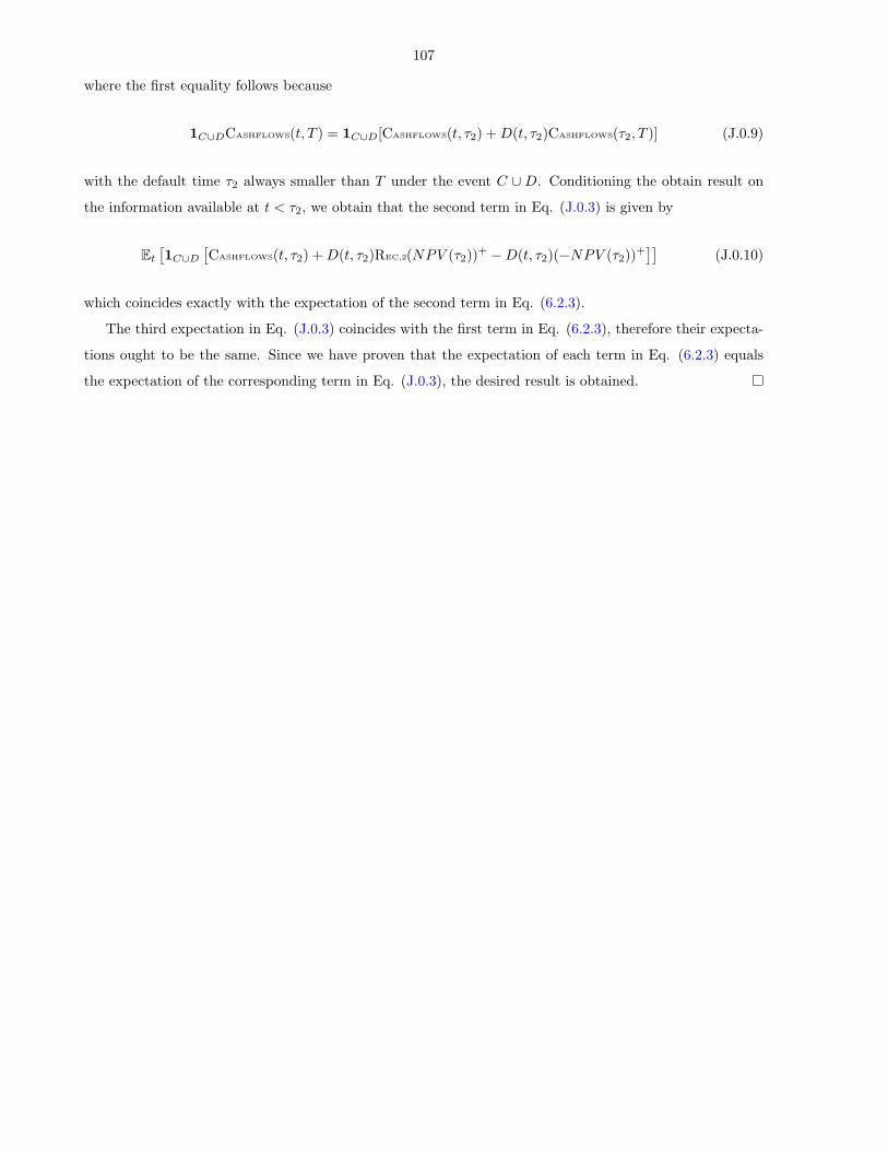
107
where the first equality follows because
1C∪DCASHFLOWS(t, T ) = 1C∪D[CASHFLOWS(t, τ2) +D(t, τ2)CASHFLOWS(τ2, T )] (J.0.9)
with the default time τ2 always smaller than T under the event C ∪D. Conditioning the obtain result on
the information available at t < τ2, we obtain that the second term in Eq. (J.0.3) is given by
Et[1C∪D
[CASHFLOWS(t, τ2) +D(t, τ2)REC,2(NPV (τ2))+ −D(t, τ2)(−NPV (τ2))+
]](J.0.10)
which coincides exactly with the expectation of the second term in Eq. (6.2.3).
The third expectation in Eq. (J.0.3) coincides with the first term in Eq. (6.2.3), therefore their expecta-
tions ought to be the same. Since we have proven that the expectation of each term in Eq. (6.2.3) equals
the expectation of the corresponding term in Eq. (J.0.3), the desired result is obtained.

108
Appendix K
Chapter 6: Proof of the SurvivalProbability Formula
Proof. We have
1τ1>τ2Q(τ1 > t|Gτ2) = 1t<τ2<τ1 + 1τ2<t1τ1≥τ2E[Q(Λ1(t) < ξ1|Gτ2 , ξ1)|Gτ2 , τ1 > τ2]
= 1A + 1τ2<t1τ1≥τ2E[FΛ1(t)−Λ1(τ2)(ξ1 − Λ1(τ2))|Gτ2 , τ1 > τ2] (K.0.1)
The last step, following from the fact that the Λ1(t) < ξ1 is the same as Λ1(t) − Λ1(τ2) < ξ1 − Λ1(τ2) and
the right-hand side ξ1 −Λ1(τ2), becomes known once we condition on ξ1 and Gτ2 . Here by FΛ1(t)−Λ1(τ2), we
indicate the cumulative distribution function of the integrated (shifted) CIR process Λ1(t) − Λ1(τ2). Since
ξ1 = − log(1− U1) and τ1 = Λ−11 (ξ1), we can rewrite Eq. (K.0.1) as
1A + 1τ2<t1τ1≥τ2E[FΛ1(t)−Λ1(τ2)(− log(1− U1)− Λ1(τ2))|Gτ2 , ξ1 > Λ1(τ2)] =
= 1A + 1τ2<t1τ1≥τ2E[FΛ1(t)−Λ1(τ2)(− log(1− U1)− Λ1(τ2))|Gτ2 , − log(1− U1) > Λ1(τ2)]
= 1A + 1τ2<t1τ1≥τ2E[FΛ1(t)−Λ1(τ2)(− log(1− U1)− Λ1(τ2))|Gτ2 , U1 > 1− exp(−Λ1(τ2))]
(K.0.2)
Let us denote U1 = 1− exp(−Λ1(τ2)). Then we can rewrite Eq. (K.0.2) as
1A + 1τ2<t1τ1≥τ2
∫ 1
0
FΛ1(t)−Λ1(τ2)(− log(1− U1)− Λ1(τ2))dQ(U1 < u1|Gτ2 , U1 > U1)] =
= 1A + 1τ2<t1τ1≥τ2
∫ 1
0
FΛ1(t)(− log(1− U1))dQ(U1 < u1|Gτ2 , U1 > U1)]
= 1A + 1τ2<t1τ1≥τ2
∫ 1
U1
FΛ1(t)(− log(1− U1))dQ(U1 < u1|Gτ2 , U1 > U1)] (K.0.3)
We next need to provide a methodology to compute the conditional distribution
C1|2(u1;U2) := Q(U1 < u1|Gτ2 , τ1 > τ2) (K.0.4)
Eq. (K.0.4) may be rewritten as

109
C1|2(u1;U2) = Q(U1 < u1|U2, U1 > U1)
=Q(U1 < u1|U2)−Q(U1 < U1|U2)
1−Q(U1 < U1|U2)
=∂C1,2(u1,U2)
∂u2− ∂C1,2(U1,U2)
∂u2
1− ∂C1,2(U1,U2)∂u2
(K.0.5)
Notice that U2 is explicitly known once we condition on Gτ2 and is given by 1−exp(Λ2(τ2)). The expressions
in Eq. (K.0.5) may be computed in closed form for the Gaussian copula and are given Schonbucher (2003)
by
∂C(u, v)∂u
= Φ
x− r1,2y√1− r21,2
(K.0.6)
where x = Φ−1(u) and y = Φ−1(v), and r1,2 is the correlation between the reference credit and the counter-
party.
A similar methodology can be repeated to compute Eq. (6.3.15) and is not reproduced here.


![[Lehman Brothers] Estimating Implied Default Probabilities From Credit Bond Prices](https://img.dokumen.tips/doc/110x75/55282fa149795917048b4613/lehman-brothers-estimating-implied-default-probabilities-from-credit-bond-prices.jpg)

